8/18/2019 Spanos Giaralis Politis 8HSTAM Patras 2007

http://slidepdf.com/reader/full/spanos-giaralis-politis-8hstam-patras-2007 1/14

See discussions, stats, and author profiles for this publication at: https://www.researchgate.net/publication/257366945

Algorithmic options for joint time-frequency analysis in structural dynamics applications

CONFERENCE PAPER · JULY 2007

READS

17

3 AUTHORS, INCLUDING:

Polhronis-Thomas D Spanos

Rice University

603 PUBLICATIONS  6,750 CITATIONS 

SEE PROFILE

Agathoklis Giaralis

City University London

39 PUBLICATIONS  226 CITATIONS 

SEE PROFILE

All in-text references underlined in blue are linked to publications on ResearchGate,

letting you access and read them immediately.

Available from: Agathoklis Giaralis

Retrieved on: 04 April 2016

8/18/2019 Spanos Giaralis Politis 8HSTAM Patras 2007

http://slidepdf.com/reader/full/spanos-giaralis-politis-8hstam-patras-2007 2/14

8th HSTAM International Congress on Mechanics

Patras, 12 – 14 July, 2007

ALGORITHMIC OPTIONS FOR JOINT TIME – FREQUENCY ANALYSIS IN

STRUCTURAL DYNAMICS APPLICATIONS

Pol D. Spanos1, Agathoklis Giaralis2 and Nikolaos P. Politis3 

1L. B. Ryon Chair in Engineering

Rice University

MS 321, P.O. BOX 1892, Houston, TX 77251, U.S.A.

e-mail: spanos@rice.edu

2Department of Civil and Environmental Engineering

Rice University

Houston, TX, U.S.A.

e-mail: agavader@rice.edu 

3BP America Inc.

Houston, TX, U.S.A.

e-mail: nikolaos.politis@bp.com

Keywords: harmonic wavelets, chirplets, intrinsic modes, inelastic response, non-stationary, accelerograms

Abstract.  The purpose of this paper is to present recent research efforts by the authors supporting the

 superiority of joint time-frequency analysis over the traditional Fourier transform in the study of non-stationary

 signals commonly encountered in the fields of earthquake engineering, and structural dynamics. In this respect,

three distinct signal processing techniques appropriate for the representation of signals in the time-frequency

 plane are considered. Namely, the harmonic wavelet transform, the adaptive chirplet decomposition, and the

empirical mode decomposition, are utilized to analyze certain seismic accelerograms, and structural response

records. Numerical examples associated with the inelastic dynamic response of a seismically-excited 3-story

benchmark steel-frame building are included to show how the mean-instantaneous-frequency, as derived by the

aforementioned techniques, can be used as an indicator of global structural damage.

1 INTRODUCTIONTypical earthquake accelerograms are inherently non-stationary as their intensity and frequency content

evolve with time due to the dispersion of the propagating seismic waves. From a structural dynamics viewpoint,

capturing the time-varying dominant frequencies present in a strong ground motion record facilitates the

assessment of its structural damage potential. Furthermore, the time histories of certain structural response

quantities, such as floor displacements and inter-story drifts of a building under seismic excitation, are also

amenable to treatment as non-stationary signals. Their evolving frequency content provides valuable information

about the possible level of structural damage caused by the ground motion. Such signals call for a joint time-

frequency analysis; for it is clear that they cannot be adequately represented by the ordinary Fourier analysis

which provides only the average spectral decomposition of a signal.

During the past two decades the wavelet transform has become a potent analysis tool in data processing that

can be used, among other applications, to yield a well defined time-frequency representation of a deterministic

signal[1]

. Consequently, this transform has drawn the attention of many researchers in structural engineering and

vibration related fields[2,3]

. Alternatively, adaptive signal processing techniques can be adopted for effectively

capturing local variations of signals on the time-frequency domain[4,5,6].

In this context, the wavelet transform incorporating appropriately filtered harmonic wavelets[7]

 (HWT), the

adaptive chirplet transform[8]

 (ACT), and the empirical mode decomposition[9]

 (EMD) in conjunction with the

Hilbert transform, are employed in the present study for an analysis of certain earthquake accelerograms[3,6]

 and

structural response time series. Previously derived theoretical formulae[3,6]

 pertaining to the concept of the mean-

instantaneous-frequency[10,11]

  (MIF) are considered. Furthermore, numerical evidence, supplementing that

already available in the literature[3,6]

, is provided to reinforce the claim that tracing the MIF of critical structural

response records is an effective way for detecting and monitoring damage to constructed facilities subject to

seismic excitations. In this respect, the inelastic response of a 3-story benchmark steel-frame building[12,13]

 

exposed to two historic seismic accelerograms scaled by various factors to simulate undamaged and heavily

8/18/2019 Spanos Giaralis Politis 8HSTAM Patras 2007

http://slidepdf.com/reader/full/spanos-giaralis-politis-8hstam-patras-2007 3/14

Pol D. Spanos, Agathoklis Giaralis and Nikolaos P. Politis 

damaged conditions is considered. Joint time-frequency representations of these accelerograms and of the

associated displacement response records of the first floor of this benchmark structure as obtained by utilizing

the HWT, the ACT and the EMD, are derived along with the corresponding time-histories of the MIFs.

2 MATHEMATICAL BACKGROUND

Consider a signal x(t) in the time domain satisfying the finite energy condition

( )2

 x t dt ∞

−∞

< ∞∫ . (1)

Traditional Fourier analysis decomposes the signal  x(t)  by projecting it onto the basis of trigonometric

(sinusoid) functions with varying frequencies ω  by means of the Fourier Transform (FT), defined by the

equation

( ) ( ) i t  X x t e dt ω ω 

∞−

−∞

= ∫ . (2)

 Note that sinusoids are mapped as delta functions in the frequency domain, achieving the optimum spectral

resolution. However, they possess no localization capabilities in the time domain, being non-decaying functions

of infinite support. Therefore, the energy density spectrum  |X( ω )|2 depicts the overall frequency content of a

signal, but provides no information about the time that each frequency component was present in the signal.Obviously, alternative analyzing functions featuring finite effective support in both the time and the

frequency domain must be employed to obtain a valid distribution of the signal energy on the time- frequency

 plane. The remainder of this section refers briefly to the most pertinent of the mathematical details of the three

signal processing techniques used in the ensuing numerical analyses. In each case, analytical formulae for the

computation of the corresponding joint time-frequency representation and mean instantaneous frequency (MIF)

of the signal x(t) are included.

2.1 Wavelet spectrogram and mean instantaneous frequency via the harmonic wavelet transform

The continuous wavelet transform uses a basis of analyzing functions generated by appropriately scaling and

translating in time a single mother wavelet function. Generally, these are oscillatory functions of zero mean and

absolutely integrable and square integrable[1]

.

 Newland[14]

 introduced the special class of harmonic wavelets which are specifically defined to have a box-

shaped band limited spectrum. Two indices (m, n), are used to define their finite support in the frequency

domain and thus to control their frequency content. Later, the filtered harmonic wavelet scheme was presented

 by the same author [7]

 incorporating a Hanning window function in the frequency domain to improve the time

localization capabilities of the harmonic wavelet transform in the wavelet mean square map for a given

frequency resolution[7,15]

. In this case, the wavelet function of scale (m, n) and position (k) in the frequency

domain takes the form

( )( , ),

1 21 cos , 2 2

( )

0, elsewhere

m n k 

mm n

n m n m

ω π π ω π 

ω 

⎧   ⎛ − ⎞⎛ ⎞− ≤ ≤⎪   ⎜ ⎟⎜ ⎟Ψ =   − −⎝ ⎠⎨   ⎝ ⎠

⎪⎩

, (3)

where m and n are assumed to be positive, not necessarily integer numbers. By application of the inverse Fourier

transform in Eq. (3) one obtains its complex- valued time domain counterpart[15]

 with magnitude

( )( )

( )( , ), 2

2

sin

1

m n k 

k t n m

n mt 

k k t t n m

n m n m

π 

ψ 

π 

⎛ ⎞− −⎜ ⎟−⎝ ⎠=

⎛ ⎞⎛ ⎞ ⎛ ⎞− − − −⎜ ⎟⎜ ⎟ ⎜ ⎟⎜ ⎟− −⎝ ⎠ ⎝ ⎠⎝ ⎠

, (4)

and phase

8/18/2019 Spanos Giaralis Politis 8HSTAM Patras 2007

http://slidepdf.com/reader/full/spanos-giaralis-politis-8hstam-patras-2007 4/14

Pol D. Spanos, Agathoklis Giaralis and Nikolaos P. Politis 

( ) ( )( , ),m n k 

k t t m n

n mϕ π 

 ⎛ ⎞= − +⎜ ⎟−⎝ ⎠

. (5)

Strictly speaking, the filtered harmonic wavelets have an infinite support in the time domain as Eqs. (4) and

(5) show, but the fairly fast decay that they exhibit, leads to the definition of an effective support, so that the

function is assumed to have a finite energy whose concentration depends on (n- m), besides k.

The harmonic wavelet transform (HWT) of a signal satisfying Eq. (1) is given by the equation

( ) ( ) *

( , ), ( , ),( ) ( )

m n k m n k  w t n m x t t dt  ψ 

+∞

−∞

= − ∫ , (6)

where the symbol (*) denotes complex conjugation. Then, in analogy to standard time- frequency analysis

 procedures[11]

, the wavelet spectrogram (SP) can be defined as

2

( , ),( , )

m n k SP t wω   = .  (7)

The latter form constitutes a three-dimensional graphical direct representation of the energy of the signal  x(t) 

versus time and frequency. Treating the SP as a joint time-frequency density function, the MIF can be computed

 by the expression[3] 

( )( , )

( , )SP 

SP t d  

 MIF t SP t d  

ω 

ω 

ω ω ω 

ω ω =

∫∫

, (8)

which captures the temporal change of the mean value of the frequencies contained in the signal normalized

over the whole spectrum.

2.2 Adaptive spectrogram and mean instantaneous frequency via the chirplet decomposition

Reported by Mallat and Zhang[18]

, and Qian and Chen[8]

, the matching pursue (MP) algorithm, allows an

alternative decomposition of any signal satisfying Eq. 1 involving a linear combination of a set of analyzing

functions (dictionary)[19]

. Of particular interest is the case of a Gaussian chirplets dictionary for which the MP

yields the following adaptive chirplet transform (ACT)

( ) ( ) p p

 p

 x t A h t = ∑   (9)

of a signal x(t), with the Gaussian chirplet h p(t) herein a four- parametered function described by the equation

( )( ) ( ) ( ){ }

2 2

2 24

 p p p p

 p p

at t i t t  

i t t  p

 p

ah t e e e

 β 

ω 

π 

⎧ ⎫ ⎧ ⎫⎪ ⎪ ⎪ ⎪− − −⎨ ⎬ ⎨ ⎬ −⎪ ⎪ ⎪ ⎪⎩ ⎭ ⎩ ⎭= . (10)

This function involves scaling by the parameter α p, shifting in time and in frequency by t  p and ω p respectively,

and frequency modulating by chirprate  β  p[16]

. It attains finite support both in the time and in the frequency

domain[17], and, thus, it is capable of capturing the local characteristics of highly non-stationary signals in both

domains[4,6]

.

Furthermore, the expansion coefficients Ap are determined by solving the optimization problem

( ) ( ) ( ) ( )2

22

max , max p p

 p p p p ph h

 x t h t x t h t dt ∞

−∞

= = ∫ , (11)

where

( ) ( ) ( )

( ) ( )

1, 0

, 0

 p p p p

 p

 x t x t A h t p

 x t x t p

+   = − ≠⎧⎪⎨

= =⎪⎩. (12)

8/18/2019 Spanos Giaralis Politis 8HSTAM Patras 2007

http://slidepdf.com/reader/full/spanos-giaralis-politis-8hstam-patras-2007 5/14

Pol D. Spanos, Agathoklis Giaralis and Nikolaos P. Politis 

For the numerical implementation of the MP algorithm, a refinement scheme introduced by Yin et al.[20]

  is

adopted in the present study.

Upon decomposing the signal x(t) as above, it can be shown that a valid distribution of the signal energy in

the time-frequency domain, namely the adaptive spectrogram (AS), is given by[8] 

( )  ( ){ }   ( ) ( )

22 1

2

, 2 p p p

 p p p

t t a t t  a

 p

 p

 AS t A e eω ω β 

ω 

⎧ ⎫⎪ ⎪⎡ ⎤− − − −⎨ ⎬− −   ⎣ ⎦⎪ ⎪⎩ ⎭=   ∑ . (13)

Furthermore, the MIF can be determined independently of the AS by the expression

( )( )( )

  ( ){ }

( ){ }

2

2

2

2

2 p p

 p p

a t t 

 p p p p p

 p

 AS a t t 

 p p

 p

 A a t t e

 MIF t 

 A a e

π ω β 

π 

− −

− −

+ −

=∑

∑. (14)

2.3 Hilbert spectrum and mean instantaneous frequency via the empirical mode decomposition

The empirical mode decomposition (EMD) is another numerical algorithmic procedure for joint time-

frequency decomposition of non-stationary signals. The signal is decomposed into a finite number of non

 predefined case-specific functions, the Intrinsic Mode functions (IMFs)[5,21,22]. An IMF is defined[9] as a functionwhich satisfies the following two conditions: (a) the number of its zero crossings and the number of its extrema

must be either equal or differ by one and (b) the mean value of the local minima envelope and the local maxima

envelopes of the function must be zero.

Specifically, the EMD yields the decomposition

( ) ( ) ( ) ( )1 1

 N N 

 j j

 j j

 x t b t r t b t = =

= + ≈∑ ∑   (15)

of a signal  x(t)  obeying Eq. 1, where b j(t)  is the jth  IMF and r(t) is a non oscillatory residual function of

negligible energy which is typically left when applying the EMD to an arbitrary signal. Associated with each

IMF is the analytic signal set in polar form as[11]

 

( ) ( )  ( ) ji t 

 j j z t c t eϑ 

= , (16)

where

( ) ( ) ( )2 2

 j j jc t b t b t  = +     (17)

is the magnitude

( )  ( )

( )arctan

 j

 j

 j

b t t 

b t ϑ    =

, (18)

is the phase, and

( )  ( )1  j

 j

b sb t ds

t sπ =

−∫   (19)

is the Hilbert transform of the jth IMF.

The salient property of the IMFs is that they are mono-component signals and therefore, the instantaneous

frequency of the jth IMF at time t is appropriately defined as the derivative of the phase of its analytic signal

[10] 

8/18/2019 Spanos Giaralis Politis 8HSTAM Patras 2007

http://slidepdf.com/reader/full/spanos-giaralis-politis-8hstam-patras-2007 6/14

Pol D. Spanos, Agathoklis Giaralis and Nikolaos P. Politis 

( ) ( )  ( ) ( ) ( ) ( )

( ) ( )2 2

 j j j j

 j j

 j j

b t b t b t b t  t t 

b t b t  ω ϑ 

−= =

+

. (20)

where the dot over a symbol denotes differentiation with respect to time.

The analytic signal of the original signal x(t) involves the sum of the analytic signals of the IMF components.

That is,

( ) ( ) ( )  ( )

1 1

ˆ j

 N N i t dt  

 j j

 j j

 x t z t c t e  ω 

= =

∫= =∑ ∑ . (21)

Then the Hilbert spectrum of x defined as

( )( )   ( ) ( )( )1 1

( , ) , N N 

 x j j j j

 j j

 H t c t t c t t ω ω δ ω ω  = =

= = −∑ ∑   (22)

constitutes a time-frequency representation of the signal x(t) and is a combination of the individual Hilbert

spectra of each of the analytic IMFs. To this end, it is natural to define the MIF of the original signal as the

weighted average of the instantaneous frequencies of the individual IMFs. That is,

( )( ) ( )

( )

2

1

2

1

 N 

 j j

 j

 IMF   N 

 j

 j

c t t 

 MIF t 

c t 

ω =

=

=∑

∑. (23)

In applying the EMD technique to the signals described in the next section, the same settings for the EMD

algorithm and the same filtering schemes for the calculation of the instantaneous frequency of the IMFs were

used as in[6]

.

3 NUMERICAL RESULTS 

In recent studies[3,6,15]

, the usefulness and relative efficiency of the ACT, the HWT and the EMD to provide

information about the time-frequency characteristics of recorded strong ground motions and of inelasticresponse records of seismically excited structural systems has been addressed.

In this section, additional studies are reported in a similar context. Specifically, the El Centro (N-S

component recorded at the Imperial Valley Irrigation District substation in El Centro, California, during the

Imperial Valley, California earthquake of May 18, 1940), shown in the (b) plot of Fig. 1, and the Hachinohe (N-

S component recorded at Hachinohe City during the Takochi-oki earthquake of May 16, 1968), shown in the (b)

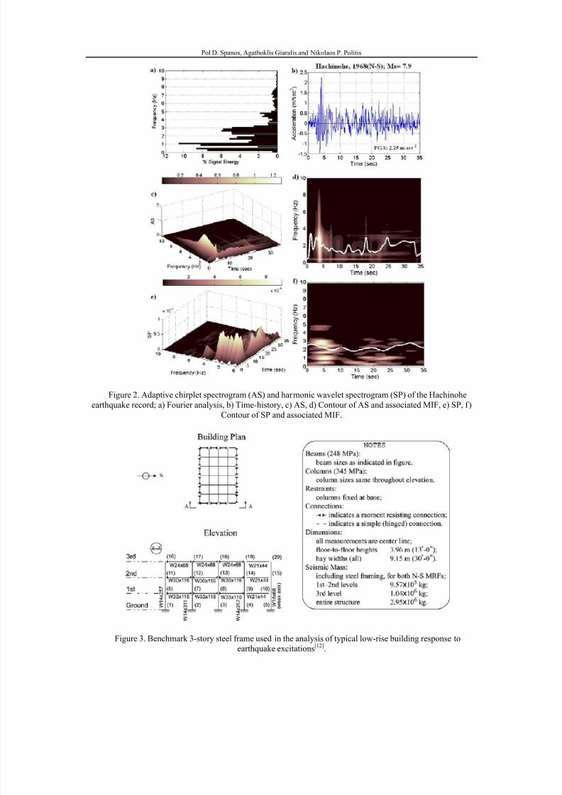
 plot of Fig. 2, earthquake records are considered. Inelastic time-history dynamic analysis was performed for the

 benchmark 3- story steel frame[12,13]

 of Fig. 3 using as input the aforementioned ground accelerations scaled by

various factors to simulate undamaged and heavily damaged conditions. The standard β-Newmark algorithm

with the assumption of constant acceleration at each time step (values β=1/4, γ=1/2), was employed for the

numerical integration in time. A trilinear hysteresis model for structural member bending was adopted[12]

.

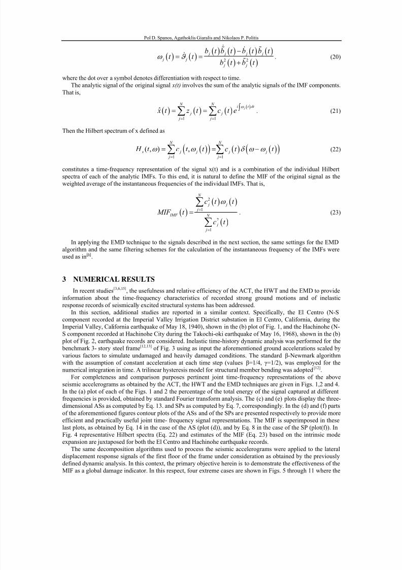
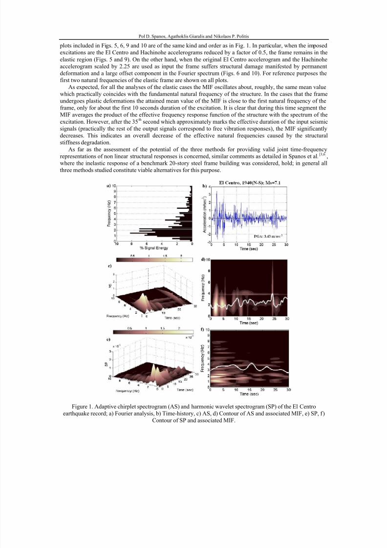
For completeness and comparison purposes pertinent joint time-frequency representations of the above

seismic accelerograms as obtained by the ACT, the HWT and the EMD techniques are given in Figs. 1,2 and 4.

In the (a) plot of each of the Figs. 1 and 2 the percentage of the total energy of the signal captured at different

frequencies is provided, obtained by standard Fourier transform analysis. The (c) and (e) plots display the three-dimensional ASs as computed by Eq. 13. and SPs as computed by Eq. 7, correspondingly. In the (d) and (f) parts

of the aforementioned figures contour plots of the ASs and of the SPs are presented respectively to provide more

efficient and practically useful joint time- frequency signal representations. The MIF is superimposed in these

last plots, as obtained by Eq. 14 in the case of the AS (plot (d)), and by Eq. 8 in the case of the SP (plot(f)). In

Fig. 4 representative Hilbert spectra (Eq. 22) and estimates of the MIF (Eq. 23) based on the intrinsic mode

expansion are juxtaposed for both the El Centro and Hachinohe earthquake records.

The same decomposition algorithms used to process the seismic accelerograms were applied to the lateral

displacement response signals of the first floor of the frame under consideration as obtained by the previously

defined dynamic analysis. In this context, the primary objective herein is to demonstrate the effectiveness of the

MIF as a global damage indicator. In this respect, four extreme cases are shown in Figs. 5 through 11 where the

8/18/2019 Spanos Giaralis Politis 8HSTAM Patras 2007

http://slidepdf.com/reader/full/spanos-giaralis-politis-8hstam-patras-2007 7/14

Pol D. Spanos, Agathoklis Giaralis and Nikolaos P. Politis 

 plots included in Figs. 5, 6, 9 and 10 are of the same kind and order as in Fig. 1. In particular, when the imposed

excitations are the El Centro and Hachinohe accelerograms reduced by a factor of 0.5, the frame remains in the

elastic region (Figs. 5 and 9). On the other hand, when the original El Centro accelerogram and the Hachinohe

accelerogram scaled by 2.25 are used as input the frame suffers structural damage manifested by permanent

deformation and a large offset component in the Fourier spectrum (Figs. 6 and 10). For reference purposes the

first two natural frequencies of the elastic frame are shown on all plots.

As expected, for all the analyses of the elastic cases the MIF oscillates about, roughly, the same mean value

which practically coincides with the fundamental natural frequency of the structure. In the cases that the frameundergoes plastic deformations the attained mean value of the MIF is close to the first natural frequency of the

frame, only for about the first 10 seconds duration of the excitation. It is clear that during this time segment the

MIF averages the product of the effective frequency response function of the structure with the spectrum of the

excitation. However, after the 35th second which approximately marks the effective duration of the input seismic

signals (practically the rest of the output signals correspond to free vibration responses), the MIF significantly

decreases. This indicates an overall decrease of the effective natural frequencies caused by the structural

stiffness degradation.

As far as the assessment of the potential of the three methods for providing valid joint time-frequency

representations of non linear structural responses is concerned, similar comments as detailed in Spanos et al.[3,6]

,

where the inelastic response of a benchmark 20-story steel frame building was considered, hold; in general all

three methods studied constitute viable alternatives for this purpose.

Figure 1. Adaptive chirplet spectrogram (AS) and harmonic wavelet spectrogram (SP) of the El Centro

earthquake record; a) Fourier analysis, b) Time-history, c) AS, d) Contour of AS and associated MIF, e) SP, f)

Contour of SP and associated MIF.

8/18/2019 Spanos Giaralis Politis 8HSTAM Patras 2007

http://slidepdf.com/reader/full/spanos-giaralis-politis-8hstam-patras-2007 8/14

Pol D. Spanos, Agathoklis Giaralis and Nikolaos P. Politis 

Figure 2. Adaptive chirplet spectrogram (AS) and harmonic wavelet spectrogram (SP) of the Hachinohe

earthquake record; a) Fourier analysis, b) Time-history, c) AS, d) Contour of AS and associated MIF, e) SP, f)

Contour of SP and associated MIF.

Figure 3. Benchmark 3-story steel frame used in the analysis of typical low-rise building response to

earthquake excitations[12]

. 

8/18/2019 Spanos Giaralis Politis 8HSTAM Patras 2007

http://slidepdf.com/reader/full/spanos-giaralis-politis-8hstam-patras-2007 9/14

Pol D. Spanos, Agathoklis Giaralis and Nikolaos P. Politis 

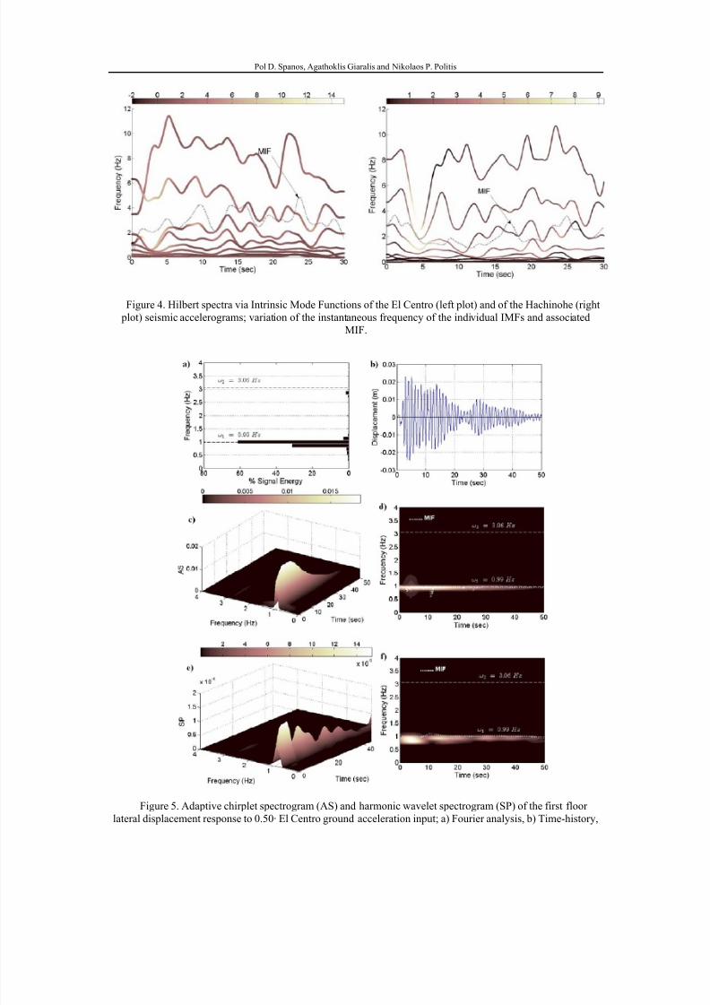
Figure 4. Hilbert spectra via Intrinsic Mode Functions of the El Centro (left plot) and of the Hachinohe (right

 plot) seismic accelerograms; variation of the instantaneous frequency of the individual IMFs and associated

MIF.

Figure 5. Adaptive chirplet spectrogram (AS) and harmonic wavelet spectrogram (SP) of the first floor

lateral displacement response to 0.50· El Centro ground acceleration input; a) Fourier analysis, b) Time-history,

8/18/2019 Spanos Giaralis Politis 8HSTAM Patras 2007

http://slidepdf.com/reader/full/spanos-giaralis-politis-8hstam-patras-2007 10/14

Pol D. Spanos, Agathoklis Giaralis and Nikolaos P. Politis 

c) AS, d) Contour of AS and associated MIF, e) SP, f) Contour of SP and associated MIF.

8/18/2019 Spanos Giaralis Politis 8HSTAM Patras 2007

http://slidepdf.com/reader/full/spanos-giaralis-politis-8hstam-patras-2007 11/14

Pol D. Spanos, Agathoklis Giaralis and Nikolaos P. Politis 

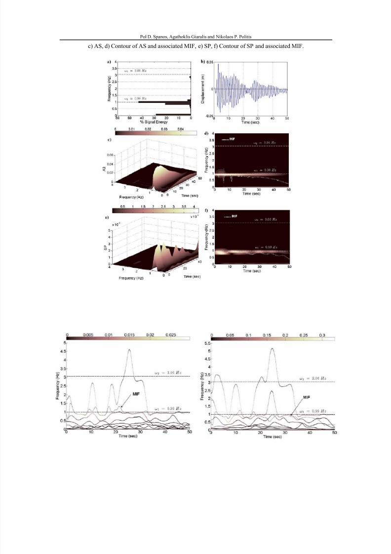
Figure 6. Adaptive chirplet spectrogram (AS) and harmonic wavelet spectrogram (SP) of the first floor lateral

displacement response to 1.00· El Centro ground acceleration input; a) Fourier analysis, b) Time-history, c) AS,

d) Contour of AS and associated MIF, e) SP, f) Contour of SP and associated MIF.

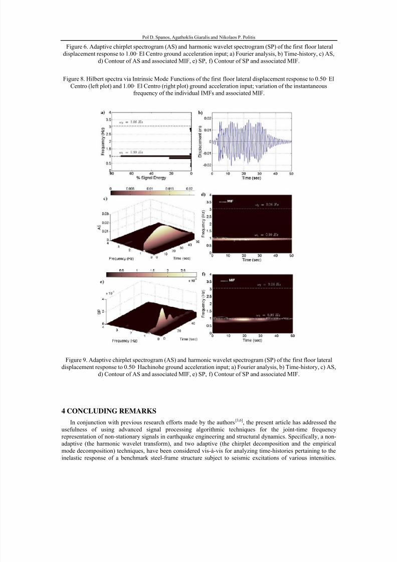
Figure 8. Hilbert spectra via Intrinsic Mode Functions of the first floor lateral displacement response to 0.50· El

Centro (left plot) and 1.00· El Centro (right plot) ground acceleration input; variation of the instantaneous

frequency of the individual IMFs and associated MIF.

Figure 9. Adaptive chirplet spectrogram (AS) and harmonic wavelet spectrogram (SP) of the first floor lateral

displacement response to 0.50· Hachinohe ground acceleration input; a) Fourier analysis, b) Time-history, c) AS,

d) Contour of AS and associated MIF, e) SP, f) Contour of SP and associated MIF.

4 CONCLUDING REMARKS

In conjunction with previous research efforts made by the authors[3,6]

, the present article has addressed the

usefulness of using advanced signal processing algorithmic techniques for the joint-time frequency

representation of non-stationary signals in earthquake engineering and structural dynamics. Specifically, a non-

adaptive (the harmonic wavelet transform), and two adaptive (the chirplet decomposition and the empirical

mode decomposition) techniques, have been considered vis-à-vis for analyzing time-histories pertaining to the

inelastic response of a benchmark steel-frame structure subject to seismic excitations of various intensities.

8/18/2019 Spanos Giaralis Politis 8HSTAM Patras 2007

http://slidepdf.com/reader/full/spanos-giaralis-politis-8hstam-patras-2007 12/14

Pol D. Spanos, Agathoklis Giaralis and Nikolaos P. Politis 

Special attention has been given to the concept of the mean instantaneous frequency (MIF) which is inherent to

these analyses, and mathematical formulae have been included to facilitate its numerical computation.

It has been found that in the cases where the frame under consideration was forced to exhibit non-linear

 behavior, the attained values of the MIF were significantly reduced compared to the cases where the frame

remained in the elastic region. In this regard, it has been shown that monitoring the mean instantaneous

frequency of records of critical structural responses in the context of a time-frequency analysis can be regarded

as an effective tool for global structural damage detection, as has been proposed before[3,6]

. The latter stems from

the ability of the techniques considered herein to capture the influence of nonlinearity on the evolution of theeffective natural frequencies of yielding structural systems during a strong ground motion event.

8/18/2019 Spanos Giaralis Politis 8HSTAM Patras 2007

http://slidepdf.com/reader/full/spanos-giaralis-politis-8hstam-patras-2007 13/14

Pol D. Spanos, Agathoklis Giaralis and Nikolaos P. Politis 

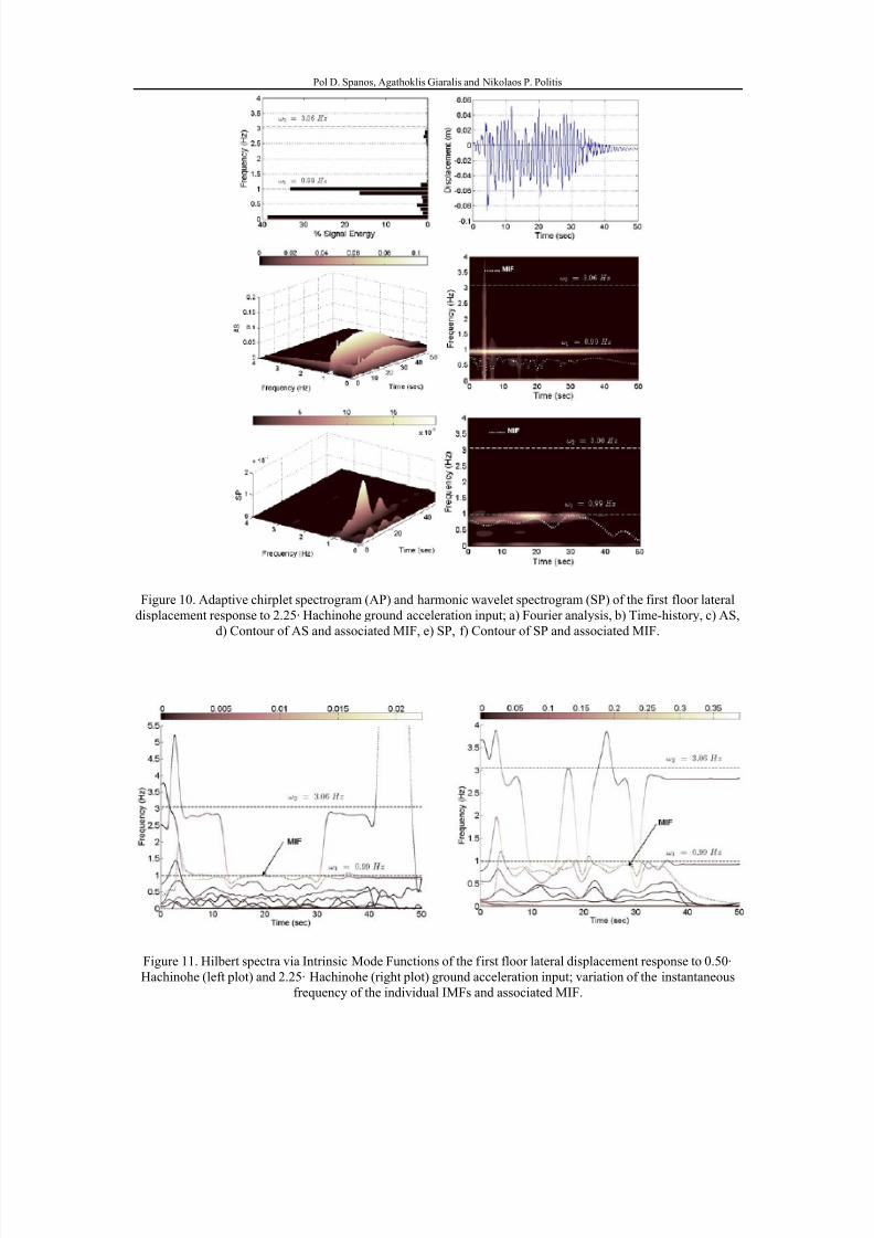
Figure 10. Adaptive chirplet spectrogram (AP) and harmonic wavelet spectrogram (SP) of the first floor lateral

displacement response to 2.25· Hachinohe ground acceleration input; a) Fourier analysis, b) Time-history, c) AS,

d) Contour of AS and associated MIF, e) SP, f) Contour of SP and associated MIF.

Figure 11. Hilbert spectra via Intrinsic Mode Functions of the first floor lateral displacement response to 0.50·

Hachinohe (left plot) and 2.25· Hachinohe (right plot) ground acceleration input; variation of the instantaneous

frequency of the individual IMFs and associated MIF.

8/18/2019 Spanos Giaralis Politis 8HSTAM Patras 2007

http://slidepdf.com/reader/full/spanos-giaralis-politis-8hstam-patras-2007 14/14

Pol D. Spanos, Agathoklis Giaralis and Nikolaos P. Politis 

ACKNOWELEDGEMENTS

The financial support of this work from an NSF grant is gratefully acknowledged.

REFERENCES

[1] Mallat, S. (1998), A Wavelet Tour of Signal Processing, Academic Press, London.

[2] Spanos, P.D. and Failla, G. (2005), “Wavelets: Theoretical concepts and vibrations related applications,”

Shock Vib. Digest, 37, pp. 359-375.[3] Spanos, P.D., Giaralis, A., Politis, N.P. and Roessett, J.M. (2007), “Numerical treatment of seismic

accelerograms and of inelastic seismic structural responses using harmonic wavelets,” Comput. Aided Civil

Infrastruct. Eng. 22, pp. 254-264.

[4] Qian, S. (2001), Introduction to time-frequency and wavelet transforms, Prentice- Hall, New Jersey.

[5] Huang, N.E. and Attoh-Okine, N.O., eds. (2005), The Hilbert-Huang transform in engineering, CRC Press,

Boca Raton.

[6] Spanos, P.D., Giaralis, A. and Politis, N.P. (2007), “Time- frequency representation of earthquake

accelerograms and inelastic structural response records using the adaptive chirplet decomposition and

empirical mode decomposition,” Soil Dynam. Earthquake Eng. 27, pp. 675-689.

[7] Newland, D.E. (1999), “Ridge and phase identification in the frequency analysis of transient signals by

harmonic wavelets,” J. Vib. Acoust. 121, pp. 149-155.

[8] Qian, S. and Chen, D. (1994), “Signal representation via adaptive normalized Gaussian functions,” Signal

Process 36, pp. 1-11.

[9] Huang, N.E., Shen, Z., Long, S.R., Wu, M.C., Shih, H.H., Zheng, Q., Yen, N.C., Tung, C.C. and Liu, H.H.(1998), “The empirical mode decomposition and the Hilbert spectrum for nonlinear and non-stationary time

series analysis,” Proc. R. Soc. Lond. A 454, pp. 903-995.

[10] Boashash, B. (1992), “Estimating and interpreting the instantaneous frequency of a signal. I.

Fundamentals,” Proc. IEEE, 80, pp. 520-538.

[11] Cohen, L. (1995), Time- Frequency Analysis, Prentice- Hall, New Jersey.

[12] Ohtori, Y., Christenson, R.E., Spencer, B.F.J. and Dyke, S.J. (2004), “Benchmark structural control

 problems for seismically excited nonlinear buildings,” J. Eng. Mech. 130, pp. 366-385.

[13] Spencer, B.F.J., Christenson, R.E. and Dyke, S.J. (1999), “Next generation benchmark control problems for

seismically excited buildings,” Proceedings of the 2nd World Conference on Structural Control . Vol.2, pp.

1135–1360, Wiley, New York.

[14] Newland, D.E. (1994), “Harmonic and musical wavelets,” Proc. R. Soc. Lond. A 444, pp. 605-620.

[15] Spanos, P.D., Tezcan, J. and Tratskas, P. (2005), “Stochastic processes evolutionary spectrum estimation

via harmonic wavelets,” Comput. Methods Appl. Mech. Eng. 194, pp. 1367-1383.

[16] Mann, S. and Haykin, S. (1995), “The chirplet transform: Physical considerations,” IEEE Trans SignalProcess. 43, pp. 2745-2761.

[17] Baraniuk, R.G. and Jones, D.L. (1996), “Wigner- based formulation of the chirplet transform,” IEEE Trans

Signal Process. 44, pp. 3129-3135.

[18] Mallat, S. and Zhang, Z. (1993), “Matching pursuits with time-frequency dictionaries,” IEEE Trans Signal

Process 41, pp. 3397-3415.

[19] Chen, S.S., Donoho, D.L. and Saunders, M.A. (1998), “Atomic decomposition by basis pursuit,” SIAM J.

Sci Comput 20, pp. 33-61.

[20] Yin, Q., Qian, S. and Feng, A. (2002), “A fast refinement for adaptive gaussian chirplet decomposition,”

IEEE Trans Signal Process 50, pp. 1298-1306.

[21] Rilling, G., Flandrin, P. and Goncalves, P. (2003), “On empirical mode decomposition and its algorithms,”

 IEEE-EURASIP Workshop on nonlinear signal and image processing  NSIP-03, GRADO(I).

[22] Flandrin, P. and Goncalves, P. (2004), “Empirical mode decompositions as data-driven wavelet-like

expansions,” Int. J. Wavelets Multiresolut. Inform. Process. 2, pp. 477-496.