Start

B

C

A

E

D

F

G

Finish

Q. 9 – 3

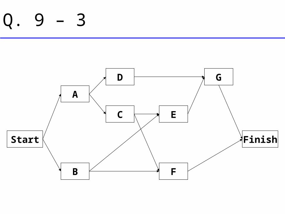
Q. 9 – 4 a.

Start Finish

40A

404

60B

716

64C

752

104D

1046

96F

15123

96E

1073

1510G

15105

Critical Path: A-D-G Completion Time = 15

Q. 9 – 4 b.

The critical path activities require 15

months to complete. Thus the project

should be completed in 1.5 years.

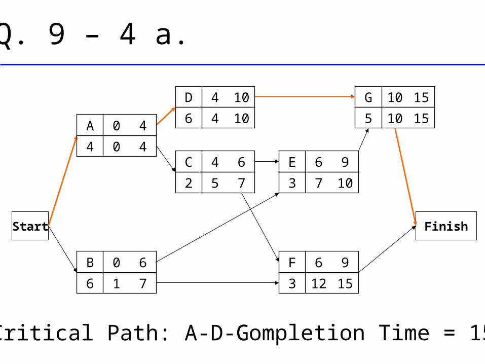
Q. 9 – 10 b.

Activity OptimisticMost

ProbablePessimistic

Expected Times

Variance

A 4 5.0 6 5.00 0.11

B 8 9.0 10 9.00 0.11

C 7 7.5 11 8.00 0.44

D 7 9.0 10 8.83 0.25

E 6 7.0 9 7.17 0.25

F 5 6.0 7 6.00 0.11

Q. 9 – 10 b.

Critical activities: B-D-F

Expected completion time: 9 + 8.83 + 6 = 23.83

Variance of projection completion time:

0.11 + 0.25 + 0.11 = 0.47

Activity OptimisticMost

ProbablePessimistic

Expected Times

Variance

A 4 5.0 6 5.00 0.11

B 8 9.0 10 9.00 0.11

C 7 7.5 11 8.00 0.44

D 7 9.0 10 8.83 0.25

E 6 7.0 9 7.17 0.25

F 5 6.0 7 6.00 0.11

Inventory Theory

How do companies use operations research to improve their inventor policy?

1. Formulate a mathematical model describing the behavior of the inventory system.

2. Seek an optimal inventory policy with respect to this model.

3. Use a computerized information processing system to maintain a record of the current inventory levels.

4. Using this record of current inventory levels, apply the optimal inventory policy to signal when and how much to replenish inventory.

The mathematical inventory models can be divided into two broad categories,

(a) Deterministic models

(b) Stochastic models

according to the predictability of demand involved.

The demand for a product in inventory is the number of units that will need to be withdrawn from inventory for some use during a specific period.

Components of Inventory Models

Some of the costs that determine this profitability are

(1) ordering costs,

(2) holding costs,

(3) Shortage costs.

Other relevant factors include

(4) revenues,

(5) salvage costs,

(6) discount rates.

The holding cost (sometimes called the storage

cost) represents all the associated with the

storage of the inventory until it is sold or used.

The holding cost can be assessed either

continuously or on a period-by-period basis.

The shortage cost (sometimes called the

unsatisfied demand cost) is incurred when the

amount of the commodity required (demand)

exceeds the available stock.

The criterion of minimizing the total (expected) discounted cost.

A useful criterion is to keep the inventory policy simple, i.e., keep the rule for indicating when to order and how much to order both understandable and easy to implement.

Lead Time:

The lead time, which is the amount of time between the placement of an order to replenish inventory and the receipt of the goods into inventory.

If the lead time always is the same (a fixed lead time), then the replenishment can be scheduled just when desired.

Deterministic Continuous-Review Models

A simple model representing the most common

inventory situation faced by manufacturers,

retailers, and wholesalers is the EOQ (Economic

Order Quantity) model. (It sometimes is also

referred to as the economic lot-size model.)

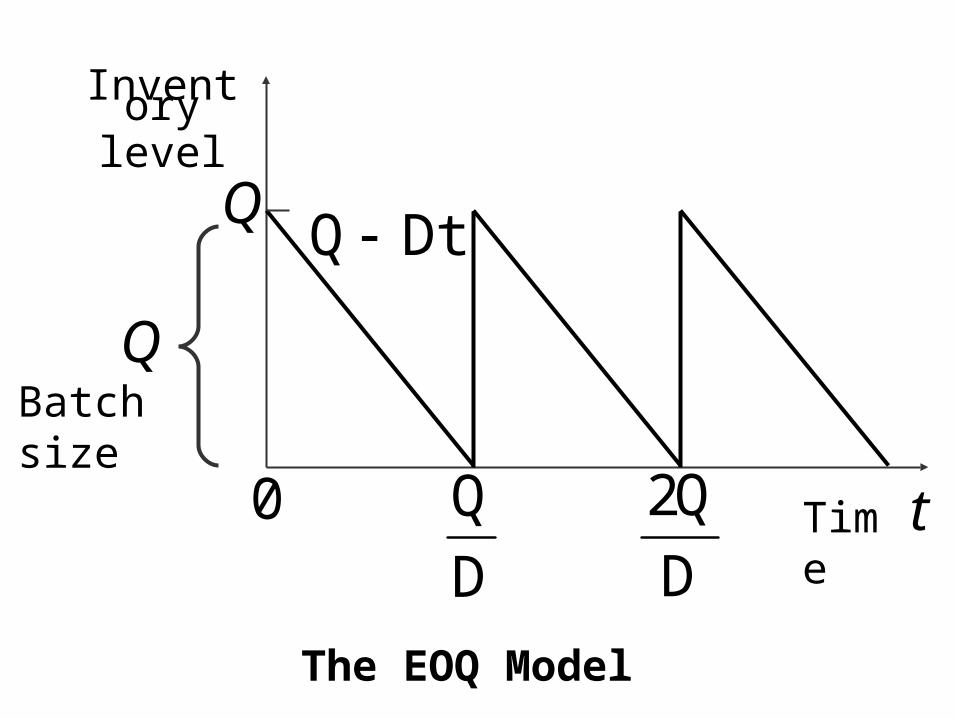
Inventorylevel

Batch size

Time

DtQ Q

Q

t0D

Q

D

Q2

The EOQ Model

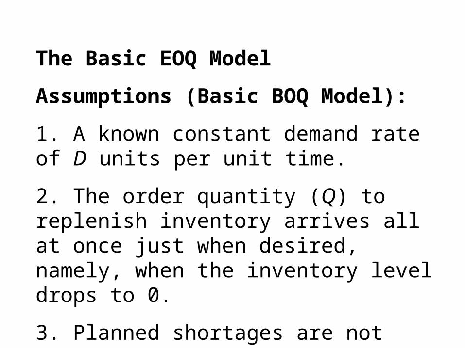
The Basic EOQ Model

Assumptions (Basic BOQ Model):

1. A known constant demand rate of D units per unit time.

2. The order quantity (Q) to replenish inventory arrives all at once just when desired, namely, when the inventory level drops to 0.

3. Planned shortages are not allowed.

I = annual holding cost rate

C = unit cost if an inventory item,

Ch = annual holding cost for one unit of time in inventory (= IC)

The objective is to determine when and how much to replenish inventory so as to minimize the total cost.

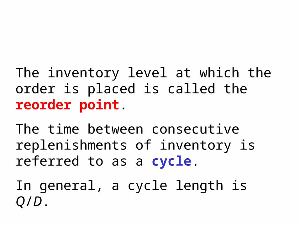
The inventory level at which the order is placed is called the reorder point.

The time between consecutive replenishments of inventory is referred to as a cycle.

In general, a cycle length is Q/D.

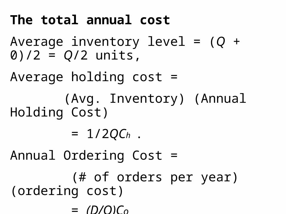
The total annual cost

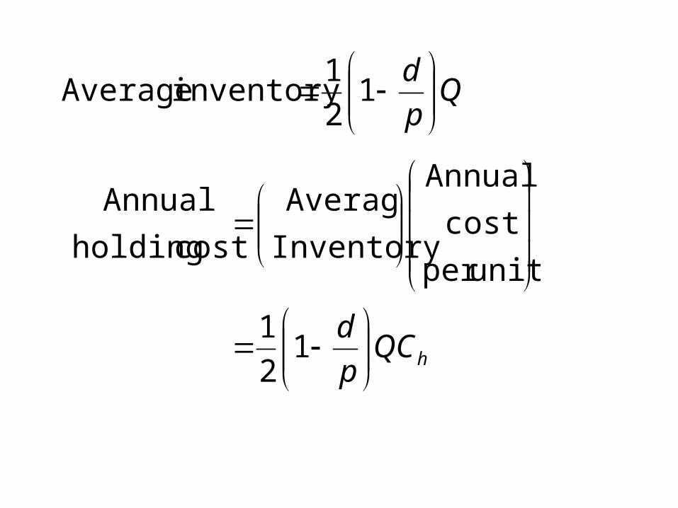
Average inventory level = (Q + 0)/2 = Q/2 units,

Average holding cost =

(Avg. Inventory) (Annual Holding Cost)

= 1/2QCh .

Annual Ordering Cost =

(# of orders per year) (ordering cost)

= (D/Q)Co

Total Annual Cost = Annual holding Cost + Annual Ordering Cost

TC = 1/2QCh+(D/Q)Co

The value of Q, say Q*, that minimizes TC,is found by setting the first derivative to zero.

which is well-known EOQ formula.

,C

DCo2*Q

h

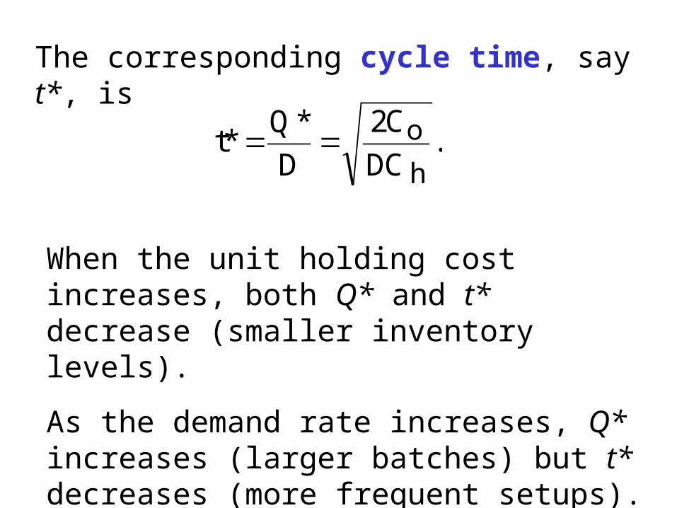
When the unit holding cost increases, both Q* and t* decrease (smaller inventory levels).

As the demand rate increases, Q* increases (larger batches) but t* decreases (more frequent setups).

The corresponding cycle time, say t*, is

.DC

C2

D

*Q*t

h

o

The EOQ Model with Planned Shortages

Planned shortages now are allowed. When a

shortage occurs, the affected customers will wait

for the product to become available again.

Their backorders are filled immediately when the

order quantity arrives to replenish inventory.

Let

S = # of Backorders

Q - S = the Max Inventory after Backorder

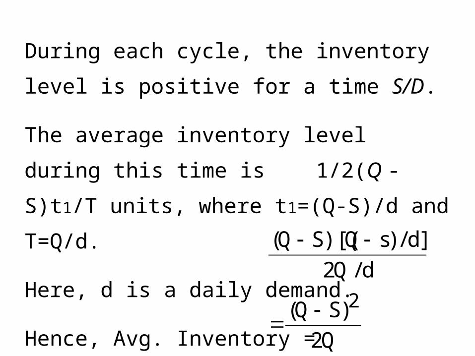
During each cycle, the inventory level is positive

for a time S/D.

The average inventory level during this time is

1/2(Q -S)t1/T units, where t1=(Q-S)/d and T=Q/d.

Here, d is a daily demand.

Hence, Avg. Inventory =

Q2

)SQ(

d/Q2

]d/)sQ)[(SQ(

2

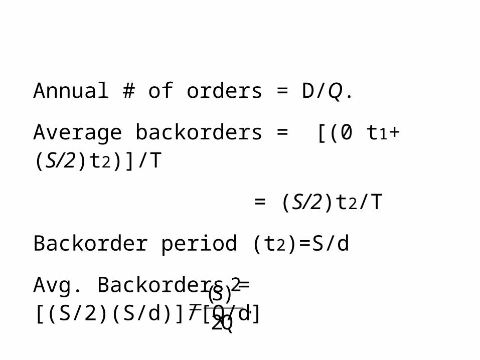
Annual # of orders = D/Q.

Average backorders = [(0 t1+ (S/2)t2)]/T

= (S/2)t2/T

Backorder period (t2)=S/d

Avg. Backorders = [(S/2)(S/d)]/[Q/d]

.Q2

)S( 2

Therefore, Total Annual Cost (TC) is

.CQ2

S

Q

DCC

Q2

)SQ(TC b

2o

h

2

Here, Ch = annual unit holding cost Co = order cost Cb = annual back order cost

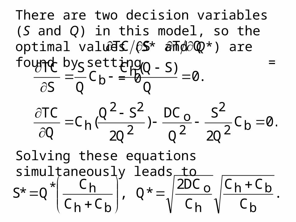
There are two decision variables (S and Q) in this model, so the optimal values (S* and Q*) are found by setting = = 0

.0CQ2

S

Q

DC)

Q2

SQ(C

Q

TC

.0Q

)SQ(CC

Q

S

S

TC

b2

2

2o

2

22

h

hb

.C

CC

C

DC2*Q,

CC

CQ*S

b

bh

h

o

bh

h*

Solving these equations simultaneously leads to

STC QT

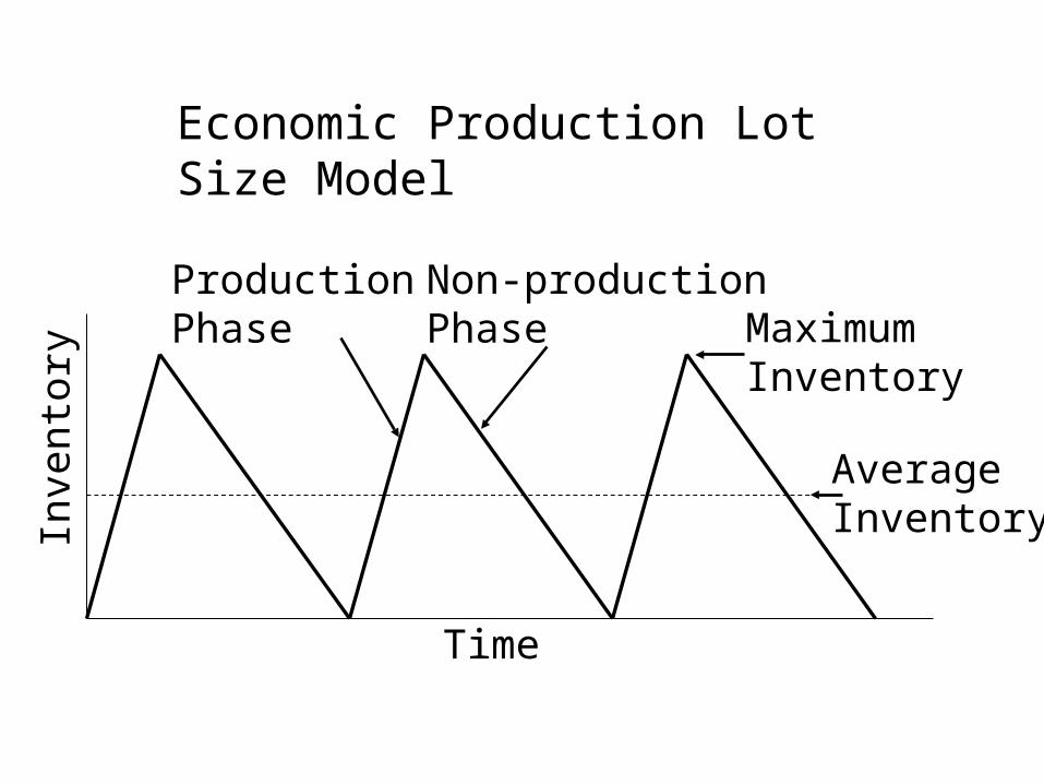
AverageInventory

MaximumInventory

Non-productionPhase

ProductionPhase

Time

Inve

ntor

y

Economic Production Lot Size Model

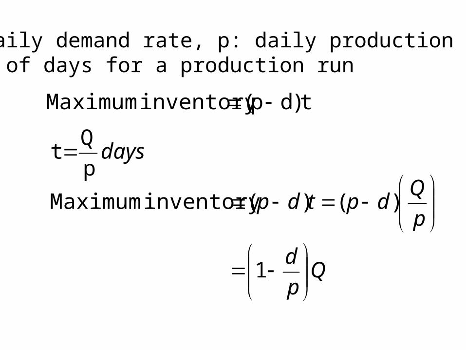
t)dp(inventory Maximum

daysp

Qt

Qp

d

p

Qdptdp

1

)()(inventory Maximum

d: daily demand rate, p: daily production ratet: # of days for a production run

Qp

d

1

2

1inventory Average

hQCp

d

12

1

unitper

cost

Annual

Inventory

Averag

cost holding

Annual

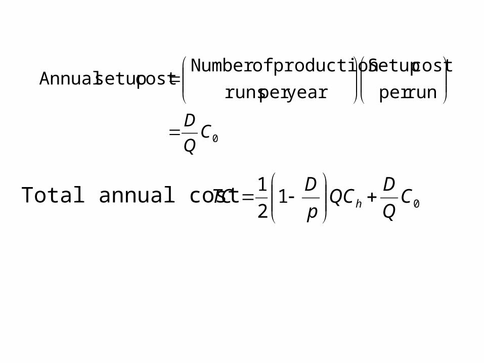
0

runper

cost Setup

yearper runs

production ofNumber cost setup Annual

CQ

D

012

1C

Q

DQC

p

DTC h

Total annual cost

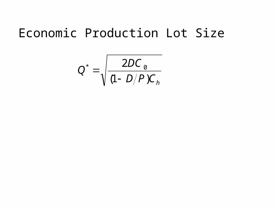
hCPD

DCQ

)1(

2 0*

Economic Production Lot Size

EMGT 501

HW Chapter 10 - 3

Chapter 10 - 7

Chapter 10 - 17

Due Day: Oct 14

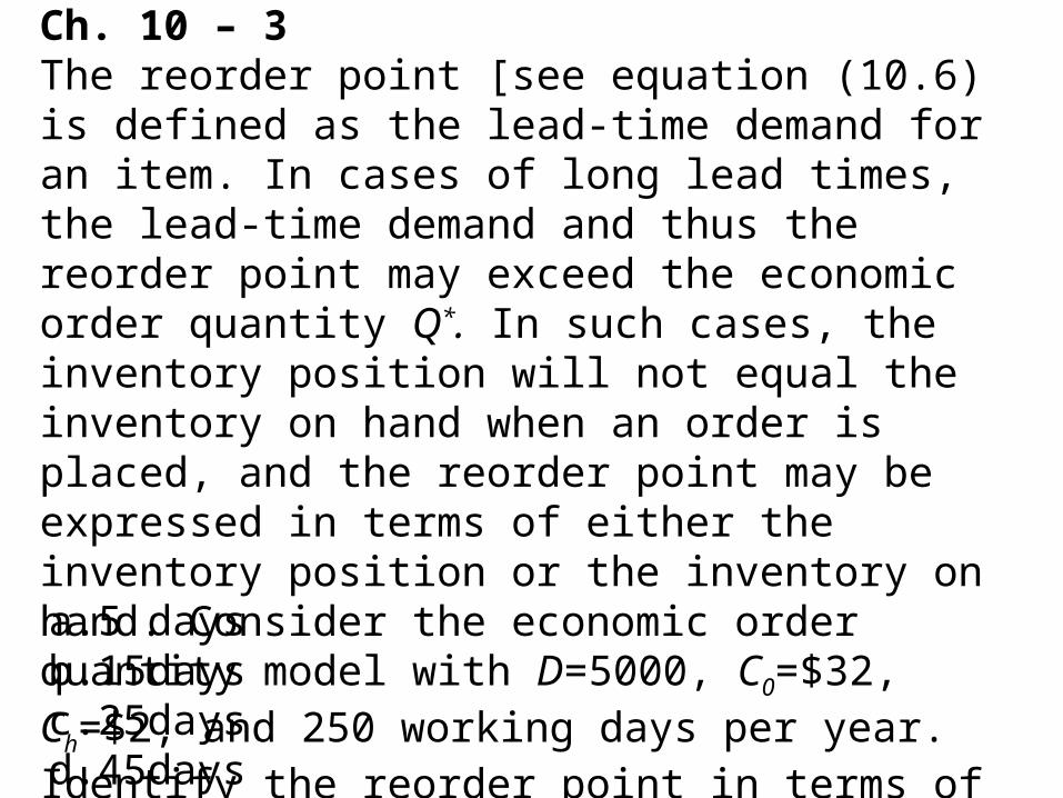
Ch. 10 – 3The reorder point [see equation (10.6) is defined as the lead-time demand for an item. In cases of long lead times, the lead-time demand and thus the reorder point may exceed the economic order quantity Q*. In such cases, the inventory position will not equal the inventory on hand when an order is placed, and the reorder point may be expressed in terms of either the inventory position or the inventory on hand. Consider the economic order quantity model with D=5000, C0=$32, Ch=$2, and 250 working days per year. Identify the reorder point in terms of the inventory position and in terms of the inventory on hand for each of the following lead times.a. 5 daysb. 15daysc. 25daysd. 45days

Ch. 10-7 A large distributor of oil-well drilling equipment operated

over the past two years with EOQ policies based on an annual holding cost rate of 22%. Under the EOQ policy, a particular product has been ordered with a Q*=80. A recent evaluation of holding costs shows that because of an increase in the interest rate associated with bank loans, the annual holding cost rate should be 27%.

a. What is the new economic order quantity for the product?b. Develop a general expression showing how the economic

order quantity changes when the annual holding cost rate is changed from I to I’.

Ch. 10-17 A manager of an inventory system believes that inventory

models are important decision-making aids. Even though often using an EOQ policy, the manger never considered a backorder model because of the assumption that backorders were “bad” and should be avoided. However, with upper management’s continued pressure for cost reduction, you have been asked to analyze the economics of a back-ordering policy for some products that can possibly be back ordered. For specific product with D=800 units per year, C0=$150, Ch=$3, and Cb =$20, what is the difference in total annual cost between the EOQ model and the planned shortage or backorder model?

If the manager adds constraints that no more than 25% of the units can be back ordered and that no customer will have to wait more than 15 days for an order, should the backorder inventory policy be adopted? Assume 250 working days per year.