Embed Size (px)
Citation preview
Chap 7-1
Chapter 7
Sampling Distributions
Statistics for Managers Using Microsoft Excel
7th Edition
Statistics for Managers Using Microsoft Excel® 7e Copyright ©2014 Pearson Education, Inc.
Chap 7-2
Learning Objectives
In this chapter, you learn: The concept of the sampling distribution
To compute probabilities related to the sample mean and the sample proportion
The importance of the Central Limit Theorem
Statistics for Managers Using Microsoft Excel® 7e Copyright ©2014 Pearson Education, Inc.
Chap 7-3
Sampling Distributions
A sampling distribution is a distribution of all of the possible values of a sample statistic for a given size sample selected from a population.
For example, suppose you sample 50 students from your college regarding their mean GPA. If you obtained many different samples of 50, you will compute a different mean for each sample. We are interested in the distribution of all potential mean GPAs we might calculate for any given sample of 50 students.
Statistics for Managers Using Microsoft Excel® 7e Copyright ©2014 Pearson Education, Inc.
DCOVA
Chap 7-4
Developing a Sampling Distribution
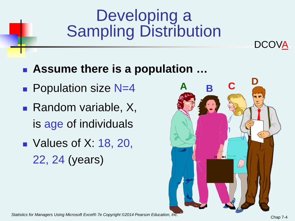
Assume there is a population … Population size N=4
Random variable, X,is age of individuals
Values of X: 18, 20,22, 24 (years)
A B C D
Statistics for Managers Using Microsoft Excel® 7e Copyright ©2014 Pearson Education, Inc.
DCOVA
Chap 7-5
.3
.2
.1
018 20 22 24A B C DUniform Distribution
P(x)
x
(continued)
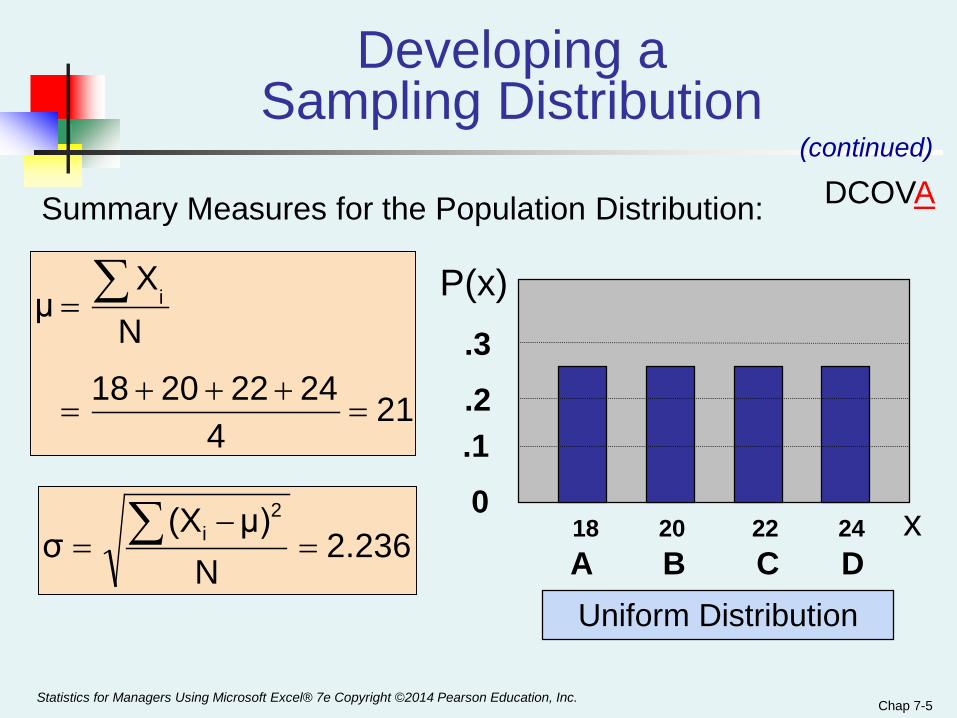
Summary Measures for the Population Distribution:
Developing a Sampling Distribution
214
24222018
NX
μ i
=+++
=
= ∑
2.236N
μ)(Xσ
2i =−
= ∑
Statistics for Managers Using Microsoft Excel® 7e Copyright ©2014 Pearson Education, Inc.
DCOVA
Chap 7-6
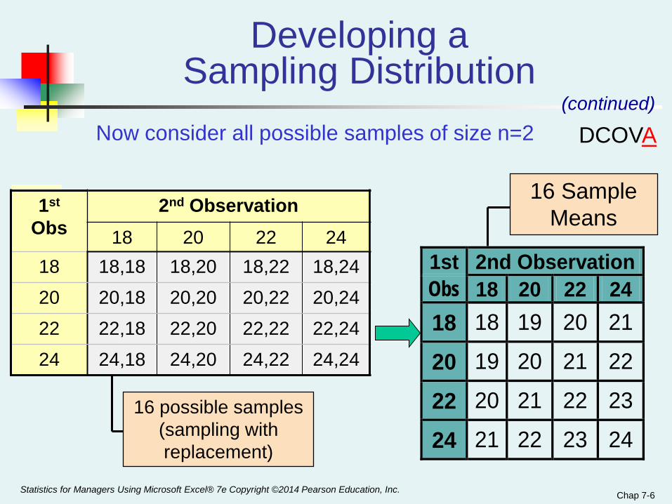
16 possible samples (sampling with replacement)
Now consider all possible samples of size n=2
1st 2nd Observation Obs 18 20 22 24 18 18 19 20 21
20 19 20 21 22
22 20 21 22 23
24 21 22 23 24
(continued)
Developing a Sampling Distribution
16 Sample Means1st
Obs2nd Observation
18 20 22 2418 18,18 18,20 18,22 18,2420 20,18 20,20 20,22 20,2422 22,18 22,20 22,22 22,2424 24,18 24,20 24,22 24,24
Statistics for Managers Using Microsoft Excel® 7e Copyright ©2014 Pearson Education, Inc.
DCOVA
Chap 7-7
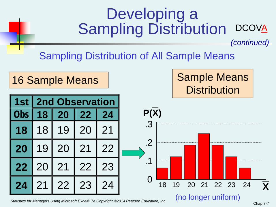
1st 2nd Observation Obs 18 20 22 24 18 18 19 20 21
20 19 20 21 22
22 20 21 22 23
24 21 22 23 24
Sampling Distribution of All Sample Means
18 19 20 21 22 23 240
.1
.2
.3 P(X)
X
Sample Means Distribution
16 Sample Means
_
Developing a Sampling Distribution
(continued)
(no longer uniform)
_
Statistics for Managers Using Microsoft Excel® 7e Copyright ©2014 Pearson Education, Inc.
DCOVA
Chap 7-8
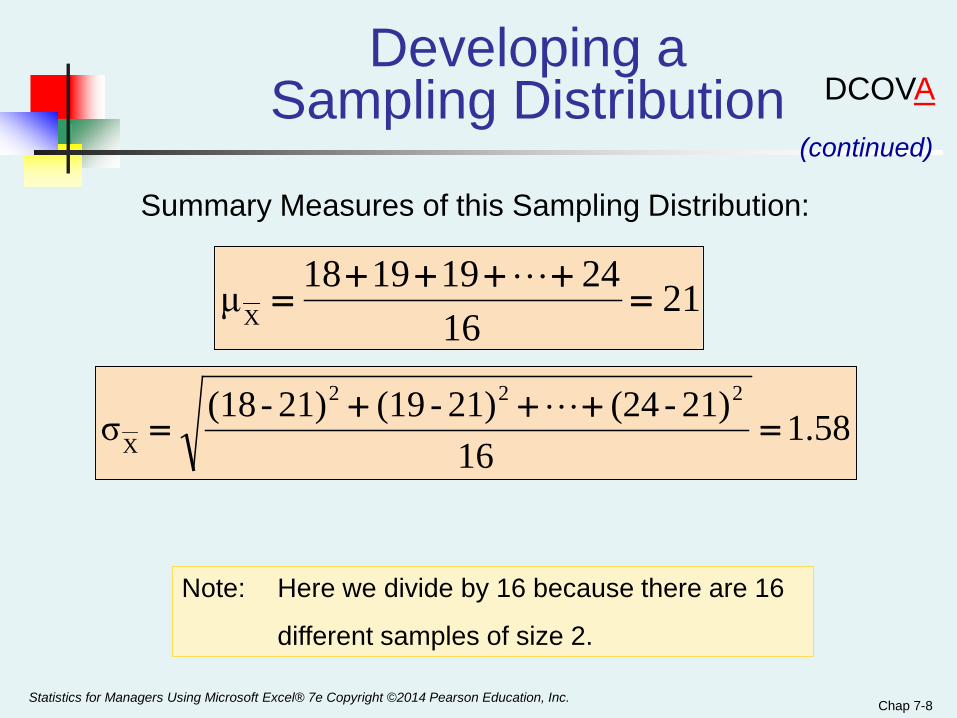
Summary Measures of this Sampling Distribution:
Developing aSampling Distribution
(continued)
2116
24191918μX =++++
=
1.5816
21)-(2421)-(1921)-(18σ222
X =+++
=
Statistics for Managers Using Microsoft Excel® 7e Copyright ©2014 Pearson Education, Inc.
DCOVA
Note: Here we divide by 16 because there are 16
different samples of size 2.
Chap 7-9
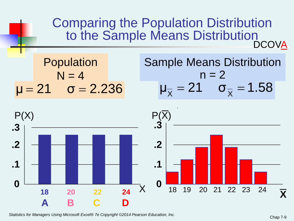
Comparing the Population Distributionto the Sample Means Distribution
18 19 20 21 22 23 240
.1
.2
.3 P(X)
X18 20 22 24A B C D
0
.1
.2
.3
PopulationN = 4
P(X)
X _
1.58σ 21μ XX ==2.236σ 21μ ==
Sample Means Distributionn = 2
_
Statistics for Managers Using Microsoft Excel® 7e Copyright ©2014 Pearson Education, Inc.
DCOVA
Chap 7-10
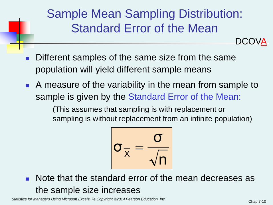
Sample Mean Sampling Distribution:Standard Error of the Mean
Different samples of the same size from the same population will yield different sample means
A measure of the variability in the mean from sample to sample is given by the Standard Error of the Mean:
(This assumes that sampling is with replacement or sampling is without replacement from an infinite population)
Note that the standard error of the mean decreases as the sample size increases
nσσX =
Statistics for Managers Using Microsoft Excel® 7e Copyright ©2014 Pearson Education, Inc.
DCOVA
Chap 7-11
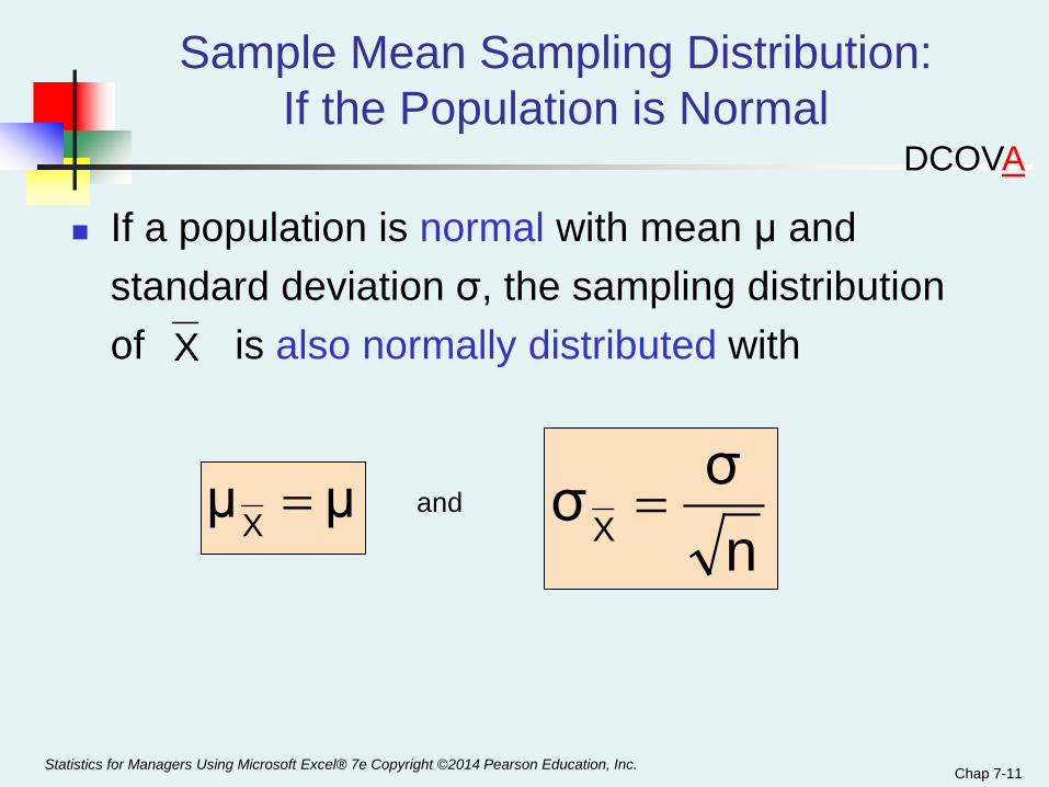
Sample Mean Sampling Distribution:If the Population is Normal
If a population is normal with mean μ and standard deviation σ, the sampling distribution of is also normally distributed with
and
X
μμX =n
σσX =
Statistics for Managers Using Microsoft Excel® 7e Copyright ©2014 Pearson Education, Inc.
DCOVA
Chap 7-12
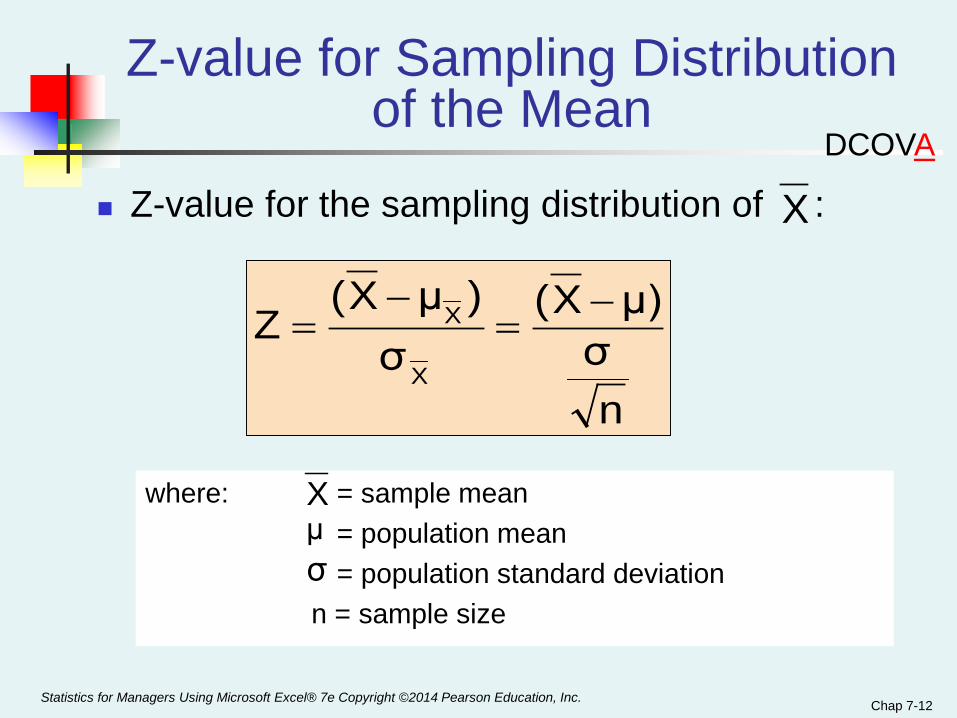
Z-value for Sampling Distributionof the Mean
Z-value for the sampling distribution of :
where: = sample mean= population mean= population standard deviation
n = sample size
Xμσ
nσ
μ)X(σ
)μX(Z
X
X −=
−=
X
Statistics for Managers Using Microsoft Excel® 7e Copyright ©2014 Pearson Education, Inc.
DCOVA
Chap 7-13
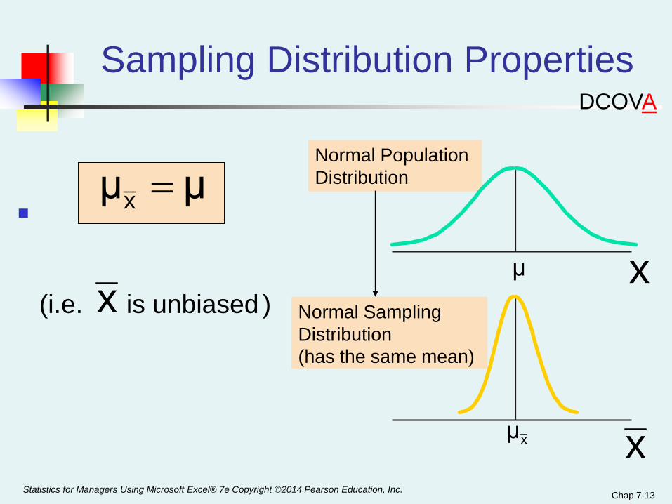
Normal Population Distribution
Normal Sampling Distribution (has the same mean)
Sampling Distribution Properties
(i.e. is unbiased )xx
x
μμx =
μ
xμ
Statistics for Managers Using Microsoft Excel® 7e Copyright ©2014 Pearson Education, Inc.
DCOVA
Chap 7-14
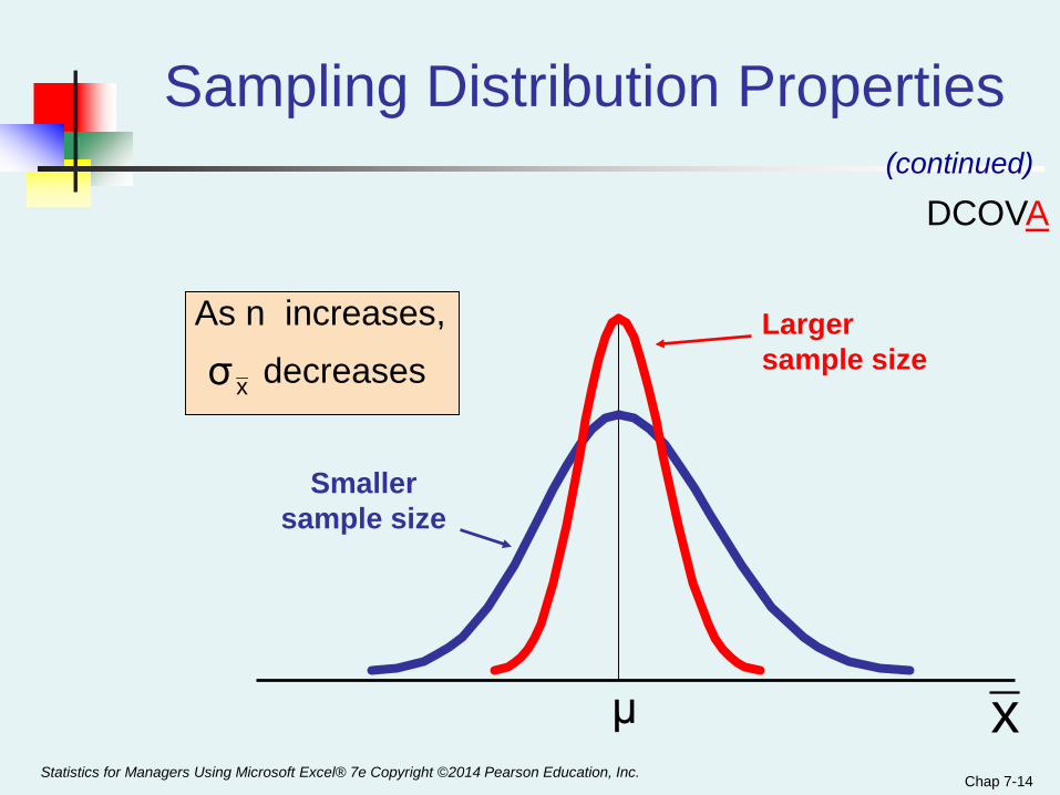
Sampling Distribution Properties
As n increases, decreases
Larger sample size
Smaller sample size
x
(continued)
xσ
μStatistics for Managers Using Microsoft Excel® 7e Copyright ©2014 Pearson Education, Inc.
DCOVA
Chap 7-15
Determining An Interval Including A Fixed Proportion of the Sample Means
Find a symmetrically distributed interval around µ that will include 95% of the sample means when µ = 368, σ = 15, and n = 25.
Since the interval contains 95% of the sample means 5% of the sample means will be outside the interval
Since the interval is symmetric 2.5% will be above the upper limit and 2.5% will be below the lower limit.
From the standardized normal table, the Z score with 2.5% (0.0250) below it is -1.96 and the Z score with 2.5% (0.0250) above it is 1.96.
Statistics for Managers Using Microsoft Excel® 7e Copyright ©2014 Pearson Education, Inc.
DCOVA
Chap 7-16
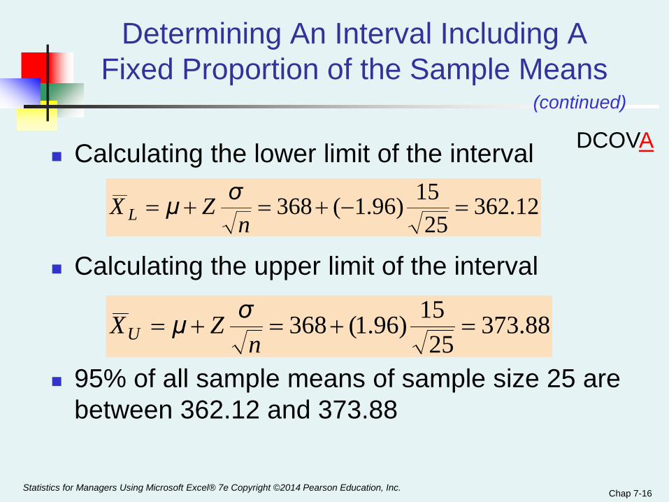
Determining An Interval Including A Fixed Proportion of the Sample Means
Calculating the lower limit of the interval
Calculating the upper limit of the interval
95% of all sample means of sample size 25 are between 362.12 and 373.88
12.36225
15)96.1(368 =−+=+=n
ZX Lσμ
(continued)
88.37325
15)96.1(368 =+=+=n
ZXUσμ
Statistics for Managers Using Microsoft Excel® 7e Copyright ©2014 Pearson Education, Inc.
DCOVA
Chap 7-17
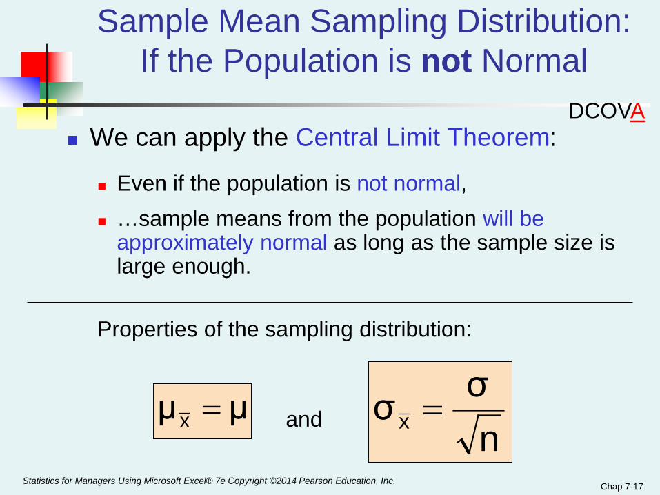
Sample Mean Sampling Distribution:If the Population is not Normal
We can apply the Central Limit Theorem:
Even if the population is not normal, …sample means from the population will be
approximately normal as long as the sample size is large enough.
Properties of the sampling distribution:
andμμx = nσσx =
Statistics for Managers Using Microsoft Excel® 7e Copyright ©2014 Pearson Education, Inc.
DCOVA
Chap 7-18
n↑
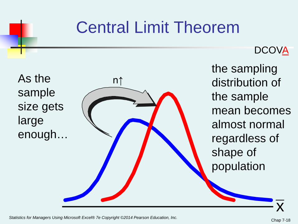
Central Limit Theorem
As the sample size gets large enough…
the sampling distribution of the sample mean becomes almost normal regardless of shape of population
xStatistics for Managers Using Microsoft Excel® 7e Copyright ©2014 Pearson Education, Inc.
DCOVA
Chap 7-19
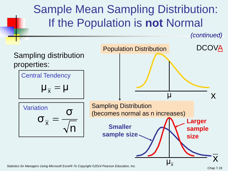
Population Distribution
Sampling Distribution (becomes normal as n increases)
Central Tendency
Variation
x
x
Larger sample size
Smaller sample size
Sample Mean Sampling Distribution:If the Population is not Normal
(continued)
Sampling distribution properties:
μμx =
nσσx =
xμ
μ
Statistics for Managers Using Microsoft Excel® 7e Copyright ©2014 Pearson Education, Inc.
DCOVA
Chap 7-20
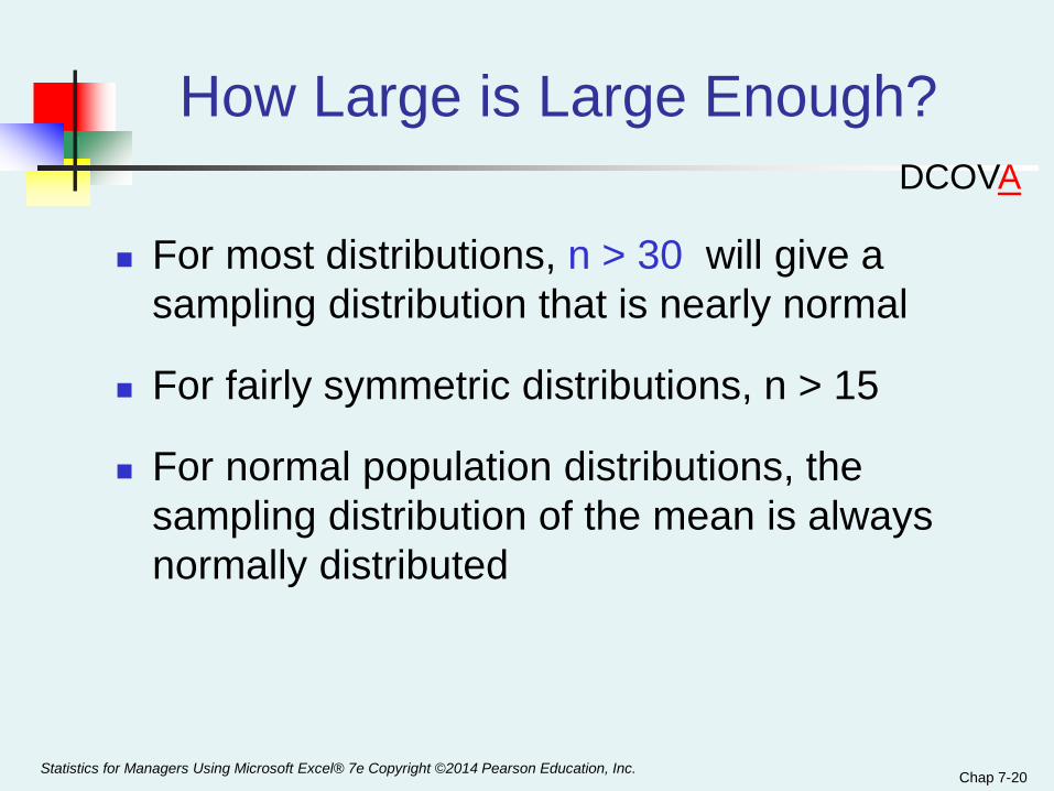
How Large is Large Enough?
For most distributions, n > 30 will give a sampling distribution that is nearly normal
For fairly symmetric distributions, n > 15
For normal population distributions, the sampling distribution of the mean is always normally distributed
Statistics for Managers Using Microsoft Excel® 7e Copyright ©2014 Pearson Education, Inc.
DCOVA
Chap 7-21
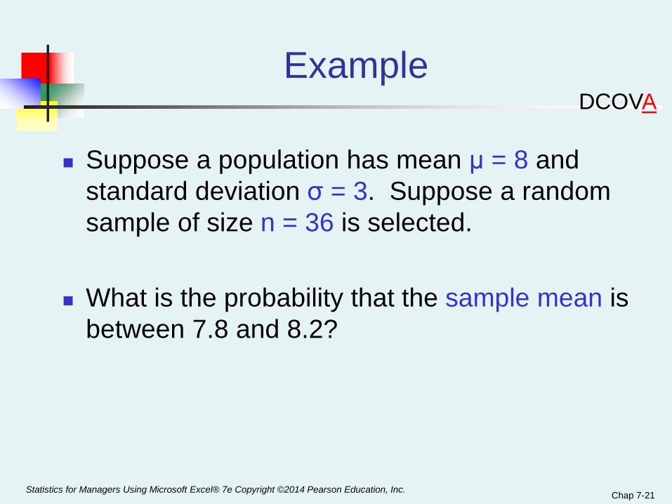
Example
Suppose a population has mean μ = 8 and standard deviation σ = 3. Suppose a random sample of size n = 36 is selected.
What is the probability that the sample mean is between 7.8 and 8.2?
Statistics for Managers Using Microsoft Excel® 7e Copyright ©2014 Pearson Education, Inc.
DCOVA
Chap 7-22
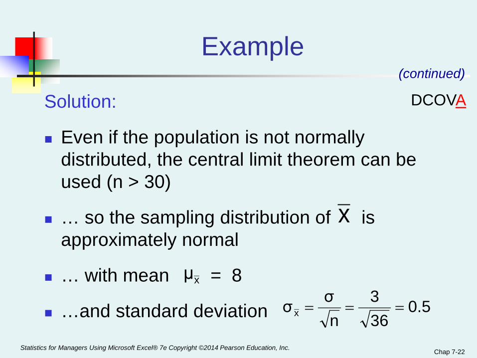
Example
Solution:
Even if the population is not normally distributed, the central limit theorem can be used (n > 30)
… so the sampling distribution of is approximately normal
… with mean = 8
…and standard deviation
(continued)
x
xμ
0.5363
nσσx ===
Statistics for Managers Using Microsoft Excel® 7e Copyright ©2014 Pearson Education, Inc.
DCOVA
Chap 7-23
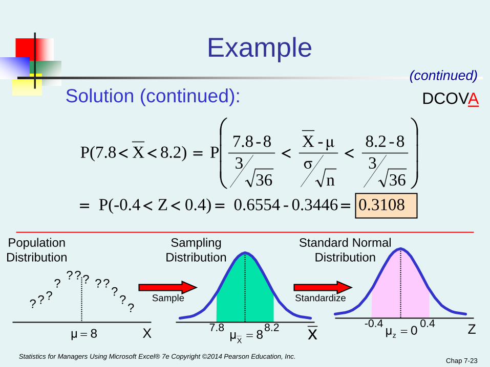
Example
Solution (continued):(continued)
0.3108 0.3446 - 0.65540.4)ZP(-0.436
38-8.2
nσ
μ- X
363
8-7.8P 8.2) X P(7.8
==<<=
<<=<<
Z7.8 8.2 -0.4 0.4
Sampling Distribution
Standard Normal Distribution
Population Distribution
??
??
?????
??? Sample Standardize
8μ = 8μX = 0μz =xXStatistics for Managers Using Microsoft Excel® 7e Copyright ©2014 Pearson Education, Inc.
DCOVA
Chap 7-24
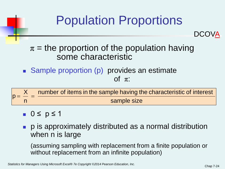
Population Proportions
π = the proportion of the population having some characteristic
Sample proportion (p) provides an estimateof π:
0 ≤ p ≤ 1
p is approximately distributed as a normal distribution when n is large(assuming sampling with replacement from a finite population or without replacement from an infinite population)
size sample interest ofstic characteri the having sample the in itemsofnumber
nXp ==
Statistics for Managers Using Microsoft Excel® 7e Copyright ©2014 Pearson Education, Inc.
DCOVA
Chap 7-25
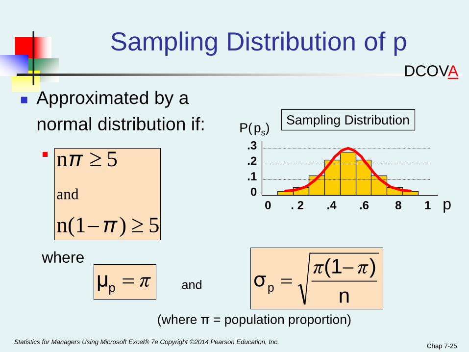
Sampling Distribution of p
Approximated by anormal distribution if:
where
and
(where π = population proportion)
Sampling DistributionP(ps).3.2.10
0 . 2 .4 .6 8 1 p
π=pμn
)(1σpππ −
=
5)n(1
5nand
≥−
≥
π
π
Statistics for Managers Using Microsoft Excel® 7e Copyright ©2014 Pearson Education, Inc.
DCOVA
Chap 7-26
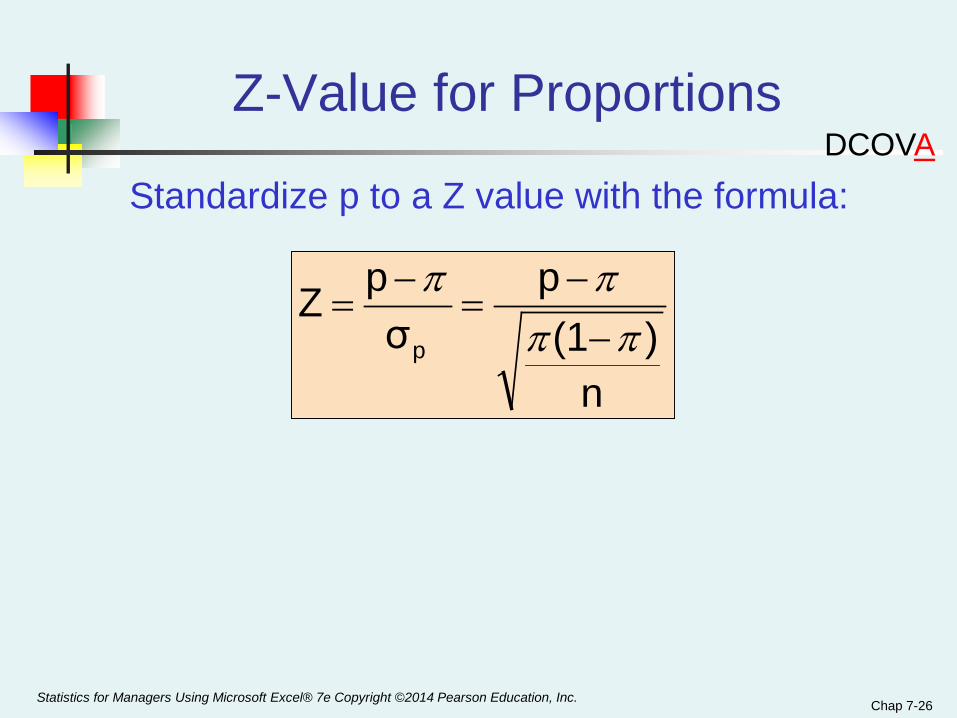
Z-Value for Proportions
n)(1
pσ
pZp ππ
ππ−
−=
−=
Standardize p to a Z value with the formula:
Statistics for Managers Using Microsoft Excel® 7e Copyright ©2014 Pearson Education, Inc.
DCOVA
Chap 7-27
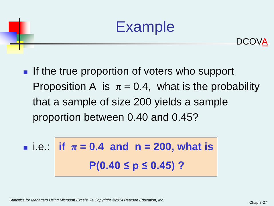
Example
If the true proportion of voters who support Proposition A is π = 0.4, what is the probability that a sample of size 200 yields a sample proportion between 0.40 and 0.45?
i.e.: if π = 0.4 and n = 200, what is
P(0.40 ≤ p ≤ 0.45) ?
Statistics for Managers Using Microsoft Excel® 7e Copyright ©2014 Pearson Education, Inc.
DCOVA
Chap 7-28
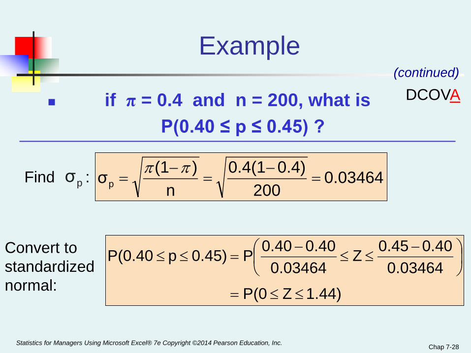
Example
if π = 0.4 and n = 200, what isP(0.40 ≤ p ≤ 0.45) ?
(continued)
0.03464200
0.4)0.4(1n
)(1σp =−
=−
=ππ
1.44)ZP(00.03464
0.400.45Z0.03464
0.400.40P0.45)pP(0.40
≤≤=
−
≤≤−
=≤≤
Find :
Convert to standardized normal:
pσ
Statistics for Managers Using Microsoft Excel® 7e Copyright ©2014 Pearson Education, Inc.
DCOVA
Chap 7-29
Example
Z0.45 1.44
0.4251
Standardize
Sampling DistributionStandardized
Normal Distribution
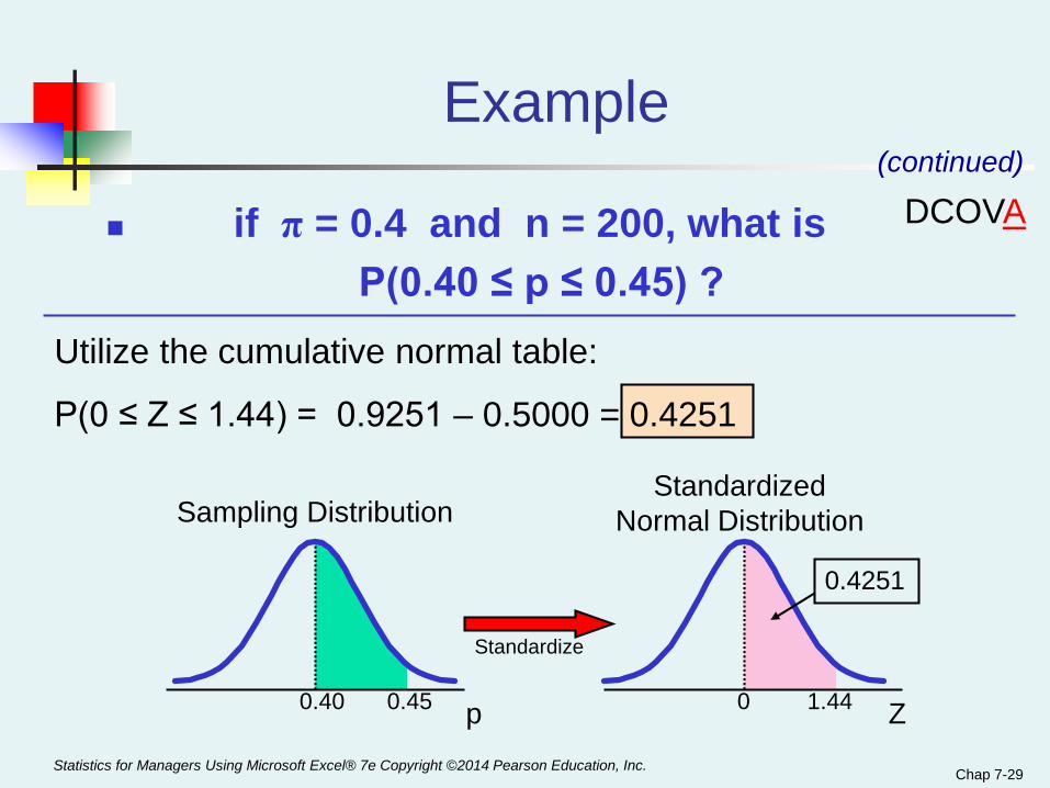
if π = 0.4 and n = 200, what isP(0.40 ≤ p ≤ 0.45) ?
(continued)
Utilize the cumulative normal table:
P(0 ≤ Z ≤ 1.44) = 0.9251 – 0.5000 = 0.4251
0.40 0pStatistics for Managers Using Microsoft Excel® 7e Copyright ©2014 Pearson Education, Inc.
DCOVA
Chap 7-30
Chapter Summary
In this chapter we discussed
Sampling distributions The sampling distribution of the mean
For normal populations Using the Central Limit Theorem
The sampling distribution of a proportion Calculating probabilities using sampling distributions
Statistics for Managers Using Microsoft Excel® 7e Copyright ©2014 Pearson Education, Inc.
Finite Populations - 1
Online Topic
Sampling From Finite Populations
Statistics for Managers Using Microsoft Excel
7th Edition
Statistics for Managers Using Microsoft Excel® 7e Copyright ©2014 Pearson Education, Inc.
Finite Populations - 2
Learning Objectives
In this topic, you learn: To know when finite population corrections are
needed
To know how to utilize finite population correction factors in calculating standard errors
Statistics for Managers Using Microsoft Excel® 7e Copyright ©2014 Pearson Education, Inc.
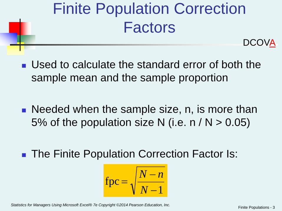
Finite Population Correction Factors
Used to calculate the standard error of both the sample mean and the sample proportion
Needed when the sample size, n, is more than 5% of the population size N (i.e. n / N > 0.05)
The Finite Population Correction Factor Is:
Finite Populations - 3Statistics for Managers Using Microsoft Excel® 7e Copyright ©2014 Pearson Education, Inc.
DCOVA
1 fpc
−−
=N
nN
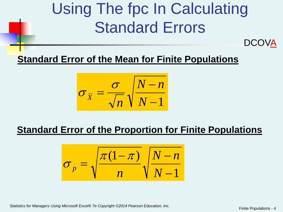
Using The fpc In Calculating Standard Errors
Finite Populations - 4Statistics for Managers Using Microsoft Excel® 7e Copyright ©2014 Pearson Education, Inc.
DCOVA
Standard Error of the Mean for Finite Populations
1−−
=N
nNnXσσ
Standard Error of the Proportion for Finite Populations
1)1(
−−−
=N
nNnpππσ
Using The fpc Reduces The Standard Error
The fpc is always less than 1
So when it is used it reduces the standard error
Resulting in more precise estimates of population parameters
Finite Populations - 5Statistics for Managers Using Microsoft Excel® 7e Copyright ©2014 Pearson Education, Inc.
DCOVA
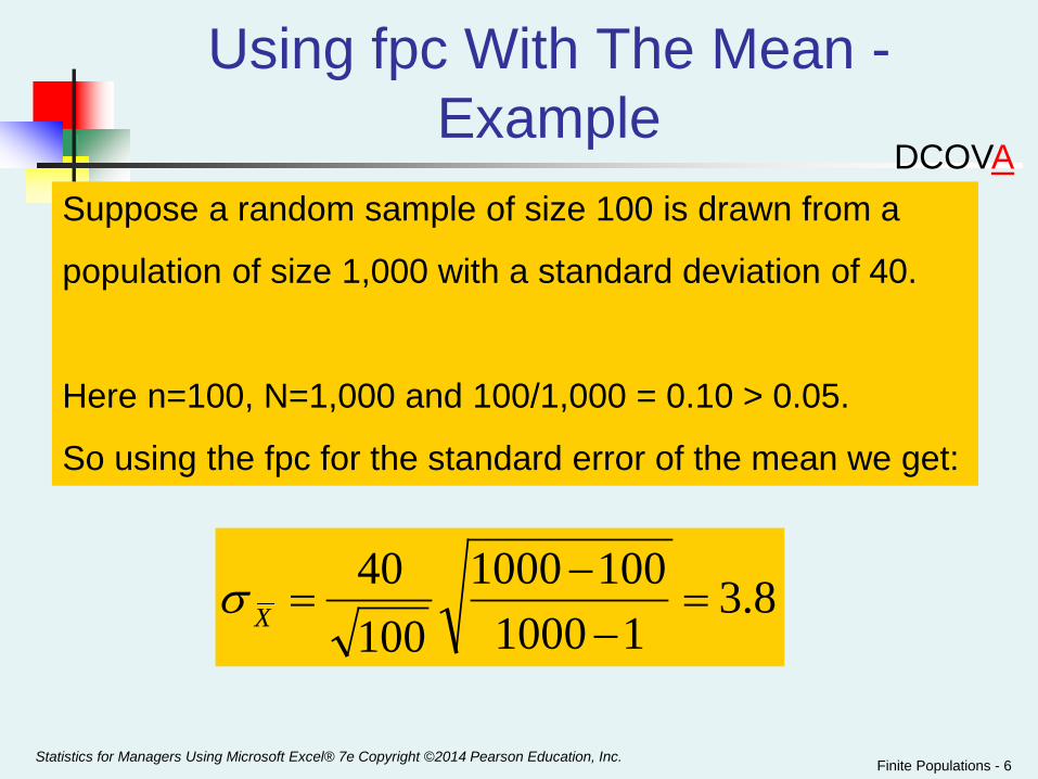
Using fpc With The Mean -Example
Finite Populations - 6Statistics for Managers Using Microsoft Excel® 7e Copyright ©2014 Pearson Education, Inc.
DCOVASuppose a random sample of size 100 is drawn from a
population of size 1,000 with a standard deviation of 40.
Here n=100, N=1,000 and 100/1,000 = 0.10 > 0.05.
So using the fpc for the standard error of the mean we get:
8.311000
100100010040
=−−
=Xσ
Finite Populations - 7
Topic Summary
In this topic we discussed
When a finite population correction should be used.
How to utilize a finite population correction factor in calculating the standard error of both a sample mean and a sample proportion
Statistics for Managers Using Microsoft Excel® 7e Copyright ©2014 Pearson Education, Inc.

Statistics for Managers Using Microsoft Excel® 7e Copyright ©2014 Pearson Education, Inc.
All rights reserved. No part of this publication may be reproduced, stored in a retrieval system, or transmitted, in any form or by any means, electronic, mechanical, photocopying, recording, or
otherwise, without the prior written permission of the publisher. Printed in the United States of America.