Embed Size (px)
Citation preview
Title Studies on Integrability for Nonlinear DynamicalSystems and its Applications
Author(s) 近藤, 弘一
Citation
Issue Date
Text Version ETD
URL http://hdl.handle.net/11094/1937
DOI
rights
Studies on Integrability for Nonlinear Dynamical Systems
and its Applications
Koichi Kondo
Division ofMathematical Science
Deparrment oflnformatics and Mathematical Science
Graduate School ofEngineering Science
Osaka University
Toyonaka, Osako 560-8531, Japan
2001
Contents
List of Figures iii
List of Tables v
Chapter1. introduction
1 . History of soliton theory
2. Integrabilityconditions
3. Integrable systems andnumerical aigorithms
4. 0utline of the thesis
1
1
2
5
7
Chapter 2. Solution and Integrability of a Generalized Derivative Nonlinear Shr6dinger
Equation
1. Introduction
2. Travelingwavesolution
3. Painlevetest
4. Numericalexperiments
5. Concludingremarks
8
8
9
12
16
22
Chapter 3. An Extension of the Steffensen Iteration and Its Computational Complexity
1. Introduction
2. The Newton method and the Steffensen method
3. TheSteffensenmethodandtheAitkentransform
4. The Shanks transform and the Åí-al gorithm
5. An extension of the Steffensen iteration
6. Convergence rate ofthe extendedSteffensen iteration
7. Numericalexamplesandcomputationalcomplexity
8. Concludingremarks
25
25
26
28
28
29
30
35
40
Chapter 4. Determinantal Solutions for Solvable Chaotic Systems and Iteration Methods
Having Higher Order Convergence Rates
1. Introduction
j
42
42
2. Trigonometricsolutionsforsolvablechaossystems
3. The Newton method and the Nourein method
4. Additionformulafortridiagonaldeterminant
5. Determinantal solution for the discrete Riccati equation
6. Determinantal solutions for hierarchy of the Newton iteration
7. Deteminantal solutions for hierarchy of the Ulam-von Neumann system
8. Determinantal solutions for hierarchy of the Steffensen iteration
9. Concludingremarks
Chapter5. ConcludingRemarks
Biblio.qraphy
List of Authors Papers Cited in the Thesis and Related Works
43
45
47
49
50
54
58
61
62
65
70
ii
List of Figures
2.1
2.2
2.3
2.4
2.5
2.6
2.7
2.8
3.1
3.2
3.3
3.4
Shape of traveling wave solution for a = 1, tu = 112 and V = 112. Solid line:
6 = O, D = O.5. Dotted line: 6 = O.91355, D = O.OOOO0976. Dashed line:
6 = O.9135528 t• • = (-1 + en) 15, D = O.
Behavior of solitary waves fora = 1,6 = O.
Behavior of solitary vvaves for a = l , 6 = O.5625.
Behavior of solitary waves fora = 1,6 = O.8.
Changes of the peaks of pulse-1 and pulse-2 after 1O times interactions.
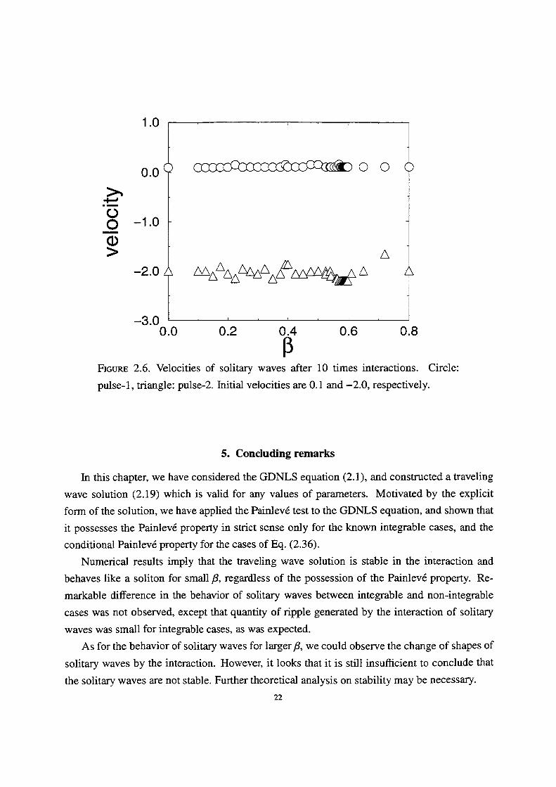
Velocities of solitary waves after 10 times interactions. Circle: pulse-1,
triangle: pulse-2. Initial velocities are O.I and -2.0, respectively.
Quantity ofposition shift (phase shift) per one interaction. Circle: pulse-1,
triangle: pulse-2.
Quantity of ripple generated after 10 times interactions. 6 v.s. ratio of
integrated values of ripple to the conserved quantity. Filled circle: the cases
of Eq. (2.28), circle: other cases.
Graphical explanation of the Steffensen iteration
A comparison of logio lf(x.)] of several iteration methods when ip'(a) s O, Å}1 .
(Example 1) Solid line: simple iteration. Dashed line: Steffensen iteration.
Circles, squares and uiangles denote the extended Steffensen iteration for
k = 2, 3, and 4, respectively.
A comparison of Iogio lf(x.)) of several iteration methods when ip'(a) = O,
ip"(a) : O. (Example2) Dashedline: Newton method. Pluses, circles,
squares and triangles denote the extended Steffensen iteration for k = l , 2, 3,
and 4, respective}y.
The parameters (t, e) for which the Newton iterations do not converge.
(Example 3)
iii
11
18
l9
20
21
22
23
24
27
37
37
38
3.5
3.6
4.I
4.2
The parameters (l, e) for which the Steffensen iterations do not converge.
(Example 3)
The parameters (l, e) for which the extended Steffensen iterations for k = 2 do
not converge. (Exarnple 3)
Behavior of the Newton method (4.6) for the case I = aobo > O.
Behavior of the Newton method (4.6) for the case I = aobo < O.
39
39
44
op
iv
2.1
3.1
3.2
3.3
List of Tables
Fluctuation of the conserved quantity Acrlo'.
Number of iterations and convergence rate. (Example 1)
Number of iterations and convergence rate. (Example 2)
Number of iterations and total numbers of mappings. (Example 3)
17
36
36
38
v
CHAPTER 1
Introduction
ln this thesis, we study integrability fornonlinear dynamical systems including differential
equations and discrete equations based on the soliton theory. Funhermore, we study applica-
tions of the soliton theory to numerical algorithms.
1. History of soliton theory
The notion of soliton means the solitary wave that travels stably and preserves its shape after
interactions. The first literature about the soliton equations was presented in 1 895 by Korteweg
and de Vries. They presented the differential equation
au au atu ;5rt +U5T.+o.3 =O (1.1)which describes the propagation of a shallow water wave. The dispersion term 03ulOx3 causes
the wave to be scattered to many waves that have different phase velocities. The nonlinear
term u Oulax varies the velocity of the wave according to the amplitude of the wave, then the
wave stands erect and soon collapses. From those reasons, it was believed that there did not exist
stable solitary wave for nonlinear evolution equations, until Korteweg and de Vries succeeded to
derive the equation that had the exact solution of solitary wave. From the balance of dispersion
and nonlinearity, the solution was obtained. The equation they presented is novvadays called the
KdV equation.
A]though the KdV equation was discovered at early year, the next development of it had
not appeared unti1 the research [89] by Zabusky and Kruskal in 1965. Using computers, they
simulated the KdV equation numerically. They set the initial condition as the superposition
of two pulses, both of vvhich were exact solutions of solitary wave of the KdV equation. They
computed a time evolution of the waves with periodic boundary condition. Two pulses moved to
same direction by different velocities, because they had different amplitudes. The higher pulse
traveled faster than the lower one. Zabusky and Kruskal observed the behaviors of interactions
of pu}ses. From the results of the experiment, they discovered that each pulse preserved its shape
and its velocity after the interactions. Moreover they discovered that positions of pulses were
shifted at the interactions. That phenomenon is called a phase shift. Solitary waves behaved
like panicles. Then they named such solitary wave as the `soliton' (a suMx `-on' stands for
i
a particle). Their numerical experiments found a new phenomenon for nonlinear evolution
equations. This discovery was also important as an example of contributions of computers to
developments of mathematics.
Next epoch-making discovery was the inverse scattering transform (IST) [23], which was
presented by Gardner, Greene, Kruskal, and Miura in 1967. By the IST, we transform a given
evolution equation to a certain linear integral equation. Then we can solve initial value problem
in principle. Another method for solving soliton equation was developed by Hirota in l970s
(cf. (29]-[38], [43], [45]). It is called Hirota 's direct method. By the direct method, we can
solve soliton equation directly not via the IST. The direct method firstly transform a given
equation to soÅíalled Hirota 's bitinearform. Then we exactly obtain exact N-soliton solution by
calculating a perturbation of the bi]inear form. That solution is also expressed as a determinant.
Such determinantal solution is called the T-function solution. And the bilinear form is reduced
to a certain identity of determinants.
The invention of the direct method also brought to us the techniques to discretize soliton
equations (cf. [39]-[42], [44]). Preserving the structure of the T-function, we do discretize the
evolution equation, the independent variable transformation, the bilinear form, and the solu-
tion, simultaneously. Such discretization is sometimes called an integrable discretization. For
example, the discrete KdV equation [39] is given by
uL'i-u:+'i =ui., -ili,;• (i •2)
Many discrete soliton equations are now presented.
In early 1980s, Sato discovered that the r-function of the Kadomtsev-Petviashvili (KP)
equation is closely related to algebraic identities such as determinant identities. Moreover, he
found that the totality of solutions for the KP equation and its higher order equations constitute
an infinite dimensional Grassmann manifold.
2. Integrability conditions
The notion of inte.qrability is rigidly defined for Hamilton systems. If a Hamilton system
of N degree of freedom has N independent and mutually involutive integrals, then the system
of ordinary differential equations (ODEs) is integrable in the sense in which the system can
be linearized in terms of successive canonical transformations. This is the main result in the
Liouville-Arnold theory. For partial differential equations (PDEs), there is no rigid definition
determined yet. However there are candidates for integrability conditions of those systems.
From studies on soliton equations, the following propenies are now accepted as definitions of
integrability for PDEs.
2
(l ) Solvability by IST.
(2) Existence of N-soliton solution.
(3) Existence of infinite number of conserved quantities or symmetries.
(4) Existence of Lax pair [53].
(5) Existence of bilinear form.
Generally it is not easy to obtain explicit solutions and conserved quantities for a given
nonlinear equation. So we want to detect whether an equation is integrable or not beforehand.
Thus the following integrability criteria have been proposed:
(a) The Painleve test for ODE.
(b) The Weiss-Tabor-Carnevale (WTC) method for PDE.
(c) The singularity confinement test for discrete equation.
(d) The algebraic entropy test for discrete equation.
Those criteria are aiso used for deciding the values of parameters of an equation that has a
possibility of integrability. We shal1 briefiy introduce them.
We first consider ODE. The singularities of a linear ODE all depend on coeMcients of the
equation. However the singularities of a nonlinear equation often depend on initial values. We
here consider a simple example
iiÅÄ/+y2=o. (1.3)
The general solution of this equation is .qiven by
1 y(x)=.-c• a4)The singularity ofy(x) occurs at x = C. Since the constant C is determined by C = -1 ly(O), the
singular point is moved according to the initial value. Such singular point is called a movable
singularpoint. lf any movable singular point of an equation is not critical point, narnely all
movable singular points are poles, then it is called that the equation has the Painleve' property.
The Painleve property is used for a criterion of integrability of ODE. We shall briefly review
the history of applications of the Painleve property.
ln 1889, Kowalevskya presented a new integrable case of the rigid body about fixed point.
The equation of motion of the rigid body is sixth order ODE with six parameters. People at that
time knew that only two cases of the equations are integrable when the parameters are special-
ized as some values. Those equations are called Euler's top and Lagrange's top respectively. In
order to solve the equation, Kowalevskya restricted the solution to no movable singular point
except for movable poles. Under that condition, she specified the parameters and succeeded to
integrate the equation. The equation she presented is now called Kowalevskya's top.
3
in 1900s, Painleve and co-workers presented soÅíalled the Painlevg equations. They inves-
tigated nonautonomous second order ODEs, and enumerated al1 equations that had no movable
critical point. They classified the equations and showed that the equations are essentially re-
duced to six types of new equations and known ones. Solutions of those six equations are called
the Painleve transcendents.
We here show how to check the Painlev6 property of a given ODE. Let a movable singu]arity
ofy(x) occur at x = C. Then we expand y(x) around the point x = C by the Laurent series
oo y(x)=(x-C)a2y, (x-C)'. (1.5) j=oWe first check whether the singularity is apole. It needs that the leading ordera is a finite
negative integer. if the leading order was a rational integer or an infinite integer, then the
singularity becarne a branch point or an essential singularity. Next we check that the Laurent
coethcients yj have enough ambiguity. It needs that the number of arbitrary constants of yj and
the initial constant C is the same as the time of differentiations of the equation. If a and yi•
satisfy those conditions and the expansion has no inconsistency, then it is said that the equation
passes the Painleve test.
We next consider PDE case. A conjecture about integrability for PDE was proposed by
Ablowitz, Ramani, and Segur [1, 2, 3]. They stated that:
Every nonlinear ODE obtained by an exact reduction of a nonlinear PDE that is
solvable by IST has the Painleve property.
Many soliton solutions are known to have this property. The KdV equation is actually reduced
to an equation of elliptic function by a reduction of traveling wave solution. The modified KdV
equation is reduced to the Painleve equation of type II by a reduction using similarity solution.
However, it is impossible to check the Painleve property of all ODEs obtained by all re-
duction of a given PDE. Thus Weiss, Tabor, and Carnevale proposed a method to check the
Painleve property of PDE directiy not via reductions. This method is called the WTC method
[84]. We briefly show the procedure of the WTC method. Let singularities of solution u(x, t)
for a nonlinear PDE occur on a manifold Åë(x, t) = O. We assume that the function ip(x, t) is an
arbitrary function, and that the solution is expressed as a formal Laurent series
co u(x, t) = ip(x, t)" Åíuj(x, t) ip(x, t)'. (1 .6)
J'--OWe check that the leading orderaisa finite negative integer, and that the number of arbitrary
functions of uj and ip is the same as the order of the differential equation. If a, u,• and ip satisfy
those conditions and the expansion has no inconsistency, then it is said that the PDE has the
4
Painlev6 property. If it is necessary to restrict uj and Åë to some conditions, then it is said that
the equation has the conditional Painleve property. An evolution equation that has a conditional
Painleve property is considered as a near-integrable system. ln this thesis, we consider stability
of such an equation.
Next we consider discrete equation. A criterion for discrete systems was first proposed by
Graimnaticos, Ramani, and Papageorgiou [25]. Their criterion is based on the property of the
singutarity confinement (SC). The SC property means that:
'Ihe singularities of a discrete system are movable, i.e., they depend on initial
conditions. And the memory of the initial conditions survives past the singularity
by a few steps.
The property of the SC is accepted as a discrete version of the Painleve property. The discrete
Painleve equations and many discrete soliton equation pass the SC test.
The SC test has been a usefu1 criterion. Hovvever, Hietarinta and Viallet presented an equa-
tion that passes the SC test but has numerically chaotic property [28]. Then they proposed a
more sensitive criterion. Their criterion is based on the algebraic entropy that is defined by the
logarithmic average of a growth of de.qrees of iterations. The algebraic entropy test and the SC
test are similar to each.
The SC type criteria are effective in reversible discrete systems such as soliton equations.
However they are ineffective in irreversib]e discrete systems. For example, the arithmetic-
harmonic mean algorithm [62],
an + bn 2anbn , bn+1= (1.7) an+! = an + bn ' 2
has the explicit solution, however does not pass the SC test. We consider in the thesis integra-
bility of such equations.
3. lntegrable systerns and numerica] algorithms
The soliton theory has been developed in mathematics, physics and engineering. The op-
tical soliton communication [26] is a famous example of app}ication of the soliton theory to
communication engi'neering. There are also applications to mathematical engjneering. A close
relationship between soliton equations and numerical algorithms has been pointed out. We
enumerate those numerical algorithms and related inte.qrable systems as follows.
e Matrix eigenvalue algorithms
- 1-step of the QR algorithm is equivalent to time 1 evolution of the ordinary Toda
equation [75] (see [73]).
5
- The LR algorithm is equivalent to the discrete Toda equation [40] (see [46]).
- The power method with the optimal shift is derived from an integrable discretiza-
tion of the Ray]eigh quotient gradient system (see [60]).
e Convergence acceleration algorithms
- The recurrence relation of the g-algorithm [85] (cf. the Shanks transform [70]) is
equivalent to the discrete potential KdV equation (see (68]).
- The p-algorithm [86] is equivalent to the discrete cylindrical KdV equation (see
[68]).
- The n-algorithm is equivalent to the discrete KdV equation (see [56]).
- The n-th term of the E-algorithm is equivalent to the solution of the discrete hun-
gry Lotka-Volterra equation (see [76]).
e Continued fraction algorithms (Pade approximations)
- The recurrence relation of the qd algorithm for calculating continued fraction is
equivalent to the discrete Toda equation.
- The ordinary Toda equation gives a method for calculating Laplace transforms via
the continued fraction (see [61]).
- A new Pade approximation algorithm is formulated by using the discrete Schur
flow (see [55]).
e Decoding algorithms
- A BCH--Goppa decoding algorithm is designed by the Toda equation over finite
fields (see [59]).
e Iteration methods having higher order convergence rate
- The recurrence relation of the arithmetic-geomeuic mean algorithm has the solu-
tion of theta function (see [18]).
- The recurrence relation of the arithmetic-harmonic mean algorithm has the solu-
tion of hyperbolic function (see I62]).
From these results, one may conjecture that a good numerical algorithm is regarded as
an integrable dynamical system. lndeed, eigenvalue algorithms and acceleration algorithms,
which are essentially linear convergent algorithms, pass the SC test of integrability criterion
(cf. {68]). Moreover, they are proved to be equivalent to discrete soliton equations via Hirota's
bilinear forms. However, some algorithms having higher order convergence rate do not pass
this integrability criterion, as we mentioned in the previous section. It needs more discussions
about inte.qrability for such equations. We consider integrabi]ity of algorithms in the thesis.
Furthermore, we develop numerical algorithms using the techniques in the soliton theory.
6
4. 0utline of the thesis
The thesis is organized as follows.
in Chapter 2, we consider a generalized derivative nonlinear Schr6dinger (GDNLS) equa-
tion. The equation is derived by adding two dispersion terms to the nonlinear Schr6dinger
(NLS) equation [51, 26], which describes a propagation of pulses in optical fibers. The GDNLS
equation has two parameters. We first construct a traveling wave solution for arbitrary values
of parameters. We next investigate integrability of the GDNLS equation by the WTC method
of the Painleve test. We show that the equation has the Painleve property and a conditional
Painleve property for some conditions of parameters. By numerical experiments, we examine
stability of the traveling wave solutions in interactions.
in Chapter 3, we consider an extension of the Steffensen method [72]. The Steffensen
method is an iteration method for finding a root of nonlinear equations. Its iteration function is
constructed without any derivative function, and it has the second order convergence rate. The
point to devise our extended method is that the iteration function is defined by using the k-th
Shanks transform which is a sequence convergence acceleration algorithm. The convergence
rate is shown to be of order k + 1 . 'Ihe use of the E-algorithm avoids the direct calculation of
Hankel determinants, which appear in the Shanks transform, and then diminishes the compu-
tational complexity. For a special case of the Kepler equation, it is shown that the numbers of
mappings are actually decreased by the use of the extended Steffensen iteration.
in Chapter 4, we give new determinantal solutions for irreversible discrete equations. The
equations considered are solvable chaotic systems and the discrete systems which are derived
from iteration methods having higher order convergence rates. We deal with the hierarchy of the
Newton type iterations (the Newton method and Nourein method [64]), that of the Steffensen
type iterations (the Steffensen method and the extended Steffensen method in Chapter 3), and
that of the Ulam-von Neumann system [77]. We obtain determinantal solutions for those sys-
tems including solvable chaotic systems in terms of addition formulas derived from some linear
systems.
In Chapter 5, we finally state some remarks and further problems.
7
CHAPTER 2
Solution and Integrability of a Generalized Derivative Nonlinear
Shr6dinger Equation
1. introduction
ln this chapter, we consider the follovving equation,
i Ut + lll uxx +lu12u+ ia lu12 u. + jic3 u2 u; =o, (2.i)
where U = U(x,t) is a complex variable and * denotes a complex conjugate. Moreover, a
and6 are real parameters. Eq. (2.1) is reduced to the well-known nonlinear Schr6dinger (NLS)
equatton
iu,+ll u,.+lul2u=o (2.2)
for a = B = O. Moreover, Eq. (2.1) yields two types of derivative nonlinear Schr6dinger
equations which are known to be integrable, namely the case of a : 6 = 1 : O [58]
iUt+;l Uxx+IUI2U+ilUl2Ux=O, (2.3)
and the case of a:fi = 2:l [83]
i Ut + llr UJwc +IUi2U+ 2i IUI2 Ux +i U2 U;l =O. (2.4)
Hereafter we cal1 Eq. (2.1 ) a generalized derivative nonlinear Schrddinger (GDNLS) equation.
We note that the GDNLS equation (2.1) can be regarded as a special case of the higher order
nonlinear Schr6dinger equation proposed by Kodama and Hasegawa [51]
i Ut + li Uxx +IUI2U+ialUl2Ux + ij3 U2 U: +i')' Ux xx =O (2.5)
which describes the pulses in optical fibers.
It is remarked that the term 1Ul2U can be eliminatedby a gauge transformation [49]. Eqs. (2.3)
and (2.4) without this term are known as the Chen-Lee-Liu (CLL) equation {15] and the Kaup-
Newell (KN) equation [50], respectively. The CLL equation was discussed by using the bilinear
formalism by Nakamura and Chen [58]. Hirota [47] bilinearized the KN equation and showed
8
that the CLL equation and the KN equation have the same bilinear forms. A class of solutions
for the CLL, KN equations and their integrable generalization by Kundu [52]
i Ut + ii Uxx +2i)' IU12 Ux + 2i('y- 1) U2 Ul +(y "- 1)('>' ny 2) IUI`U = O, (2.6)
where 7 is a real parameter, has been constructed explicitly through the bilinear formalism by
Kakei et al. [49].
We first construct a traveling wave solution ofthe GDNLS equation (2.1 ) in Section 2. Moti-
vated by a concrete form of the solution, we investigate the integrability of the GDNLS equation
by using the Painleve test in Section 3. Finally we examine a behavior of the traveling wave
solution numerically in Section 4. In Section 5, we mention several remarks of this chapter.
2. Iraveling wave so]ution
ln this section, we construct a traveling wave solution for the GDNLS equation. Here we
remark that the values of parameters a, P in Eq. (2.1) are taken to be arbitrary by the scale
change except for the ratio 61a, and hence Pla can be regarded as a characteristic parameter of
the equation.
Eq. (2. 1 ) is invariant under the following transformation
1 0(x, T) e-iV(X-XT), (2.7) U(x, t) = iNIZII
where
x= k(X-VT), t= k2T, k=l- Va+VX3 (2.8)and V is an arbitrary constant. Taldng this invariance into account, we first construct a stationary
solution. We put
U(x, t) := r(x) exp(i e(x)) exp(i tu t), (2.9)
where r(x) and e(x) are real functions in x, and tu is a real constant. Substituting (2.9) into
Eq. (2.I), we get
r.=2cor-2r3+re.? +2(a -- P)Ee. (2.10)
from the real part and
rxe. -2(a +6)rr. (2.l l) exx = -2 r 9
from the imaginary part, respectively.
solution
ex =Kr,
where K is a constant. We obtain from Eq. (2.1 l )
(2K + a + /3)rr. = O,
from which we have
a+P K=- . 2Then Eq. (2.IO) becomes
r. = 2to r - 2E - i(a +6)(3a - 5P) ".
Integrating Eq. (2.I5), we obtain
8w eÅ}2 ViEJx l
The following ansatz is crucial for our construction of
1 + 2 e'2 VMX + (1 + ica(a +P)(3a - 5P)) eÅ}4 Vthx '
Moreover, we get from Eqs. (2.12), (2.14) and (2.16)
-, fi +(1
3a- 56 tan ( 1+itu(a +P)(3a- 5P)
where the following conditions should be satisfied that
2 w2 O, 1+ sw(a +6)(3a- 56) )Ofor the reality of r and e. Substituting Eqs. (2.1 6) and (2.17) into Eq.
ary wave solution. Then, applying the transformation (2.7)-(2.8),
solution. [1ie result is expressed as
N+1 U(x• `) = ,-e.'S',,. (2--S '. gg,tol )-z" .
Here we define function ip(x, t) as
ip = Px + ;iip2t + ip(o) .
And we define parameters p, st, P, e, and N as
p = (1 - Va + V6)S:! + iV,
n=Å}V5di,
10
+ itu(a + 6)(3a - 56)) eÅ}2 VMx )•
(2.12)
(2.13)
(2.14)
(2.15)
3(a + fi)e=-
(2.16)
(2.17)
(2.1 8)
(2.9), we have the station-
we obtain the traveling wave
(2.19)
(2.20)
(2.21)
(2.22)
P= (1 - Va+ V6) (1 + S2 -g(a +6)(3a- 56) , (2.23)
e= (1 - Va+ V6) (1 -9 -g (a +6)(3a- 56) , (2.24)
3(a + fi) (2.25) N= 3a-56
and ip(O) and V are arbitrary constants, The condition (2. 1 8) is also necessary here. This solution
is characterized by the parameters cc) and V for fixed a and6. The shape of the solution varies
by the value of
D= Pe = (1 - Va+ Vfi)2 (1 + iw(a +P)(3a- 56)} . (2.26)
In fact, 1UI is given by
(p + p*)2 eptip' (2.27) IUI= 1 + 2 eip'ip' + D e2(ip+ip') '
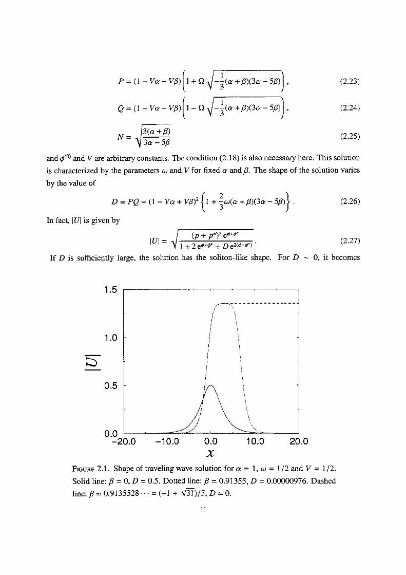
If D is suMciently large, the solution has the soliton-like shape. For D - O, it becomes
1 .5
1 .0
liii)
O.5
!
! l t y '
/1
! ' l l ' t ! t i l ' '
t'!!!'!t
l
lt.--`r..tt
x o.o -20.0 -10.0 O.O 10.0 20.0 X
FJGuRE 2.1. Shape of traveling wave solution fora = l, co = l12 and V = 112.
Solid line: 6 = O, D = O.5. Dotted line: B = O.91 355, D = O.OOOO0976. Dashed
line: 6 = O.9135528 • • • = (-1 + VIiT)15, D = o.
Il
trapezoidal shape and for D . O, it has the kink-like shape as illustrated in Figure 2.1 . Hence
the traveling wave solution (2.19) may behave as a solitary wave.
Here we remark that if we take the limit a,P . O, this solution is reduced to the l --soliton
solution of the NLS equation. Similarly, in the cases ofPla = O and61a = 112, it gi'ves the
1-soliton solution of Eqs. (2.3) and (2.4), respectively.
It should be emphasized that if N, which depends only on the ratio of a and6, is an odd
integer, the traveling wave solution (2.I9) is rational in exponential functions which is the com-
mon feature of soliton solutions. Thus it might be expected that in such cases, solitary waves of
the GDNLS equation has good propenies like that of integrable cases. The ratio of a and6 in
such cases are gi'ven by
6 3m(m+1) i= 5m(m+1)+2, M= O, 1, 2, •... (2.2s)
The cases m = O and m = 1 correspond to Eqs. (2.3) and (2.4), respectively, and they are known
to be integrable as mentioned in the introduction.
Moreover, it should be noted that the l-soliton solution for Eq. (2.6) obtained by Kakei et
al. [49] has a quite similar form to Eq. (2.19). Indeed, we can check that l-soliton solution of
equation (2.6) for 7 = O,1 equivalent to (2.19) for N = 1,3, respectively, and not for other
cases.
From the observation above, it may be natural to ask whether the cases ofm > l in Eq. (2.28)
are integrable or not. As for the integrability in a strict sense, the answer is no. In fact, Clarkson
and Cosgrove [17] investigated the Painleve property to the following equation,
iur + u.. +ia uu"u. +iic3 u2ul +7u3u'2 +6u2u' =O, (2.2g)
where a, 6, 7, and 6 are real parameters, and shown that it is integrable only the case when it
is equivalent to Eq. (2.6). However, we may expect some information from integrability test
which distinguish the cases of Eq. (2.28) from other cases. We consider the integrability of the
GDNLS equation (2.1) in the next section.
3. Painlev6 test
in this section, we investigate the integrability of the GDNLS equation by using so-called
the Painleve test proposed by Weiss et al. [84], and show that the GDNLS equation possesses
"conditional Painleve property" for the cases of Eq. (2.28).
12
Following to the procedure of the test, vve regard that u = U andv = U" are independent,
and consider the GDNLS equation as a coupled system
'1 iut +s uxx + u2v+ ia uu.v+ iic3 u2v. =O, (2.3o)
-i v, +g v..+v2u-ia vv.u •- jp v2u. =o. (2.3i)
We assume the formal Laurent expansion around the zero points of some analytic function
Åë(x, t) for the solution of Eqs. (2.30) and (2.31 )
co co u= ipaZuJ ip', v= ipb2v, ÅëJ. (2.32) J-=O j--OIn this method, if
(1) there is no movablecritical points, namely, the leading orders a and b are finite integers,
(2) the expansion (2.32) has suthcient number of arbitrary functions uJ• and vj,
(3) there is no incompatibilities in the expansion,
then it is regarded that the equation passes the Painleve test, or it is said that the equation pos-
sesses the Painleve property. In such case, it is usually believed that the equation is integrable.
We show the concrete analysis in the following.
3.1. Leading order analysis. To get the leading power a and b, we substitute u -- uo ipX
and v -- vo ipb into Eqs. (2.30) and (2.31). We obtain the relation
a+b=-1, (2.33)to adjust the leading order, and find
a-g(-iÅ} g(.a-',6i), (2.34)
3 uovo=Å}i ipx (2.35) (a + 6)(3a - 56)
Since a and b should be integers, we get the condition
6-. 3m(m+i) , m. o, i, 2, ... a 5m(m+1)+2
which is exactly the same as the condition (2.28).
I3
(236)
3.2. Resonance analysis. The degree jis called resonance when uj or vj becomes an arbi-
trary function. The recurrence relation for uj and vi• js gi'ven by
(All,b2!i,')(:i).(gl), j.o,,,2,3,.... (2.37)
Here we define elements Ai'?, Ai',b, AS',), and AS',) as
AS'? = S(j +a- 1)(j + a)ipl + i{a(j + 2a) + 26b}uo vo ip. , (2.38)
Ai',D=i{aa+6(j+b)}u3ip., (2.39) AS'?=-i{ab +p(j+a)} vg ip., (2.4o) A(,',D = S(j +b- 1)(j + b)ipl -i{a(J' + 2b) + 2)Ba}uovoÅë. . (2.41)
And we define Fj• and GJ• as some polynomials of uj, vj and ip such that
F,• = Fj(uo,.. ., u,•-,, vo,..., vj.,, Åë), (2.42)
G]- --- Gj(uo,...,uj-i,vo,...,vj-i,Åë). (2.43)
Moreover we define uj --- vj = O for j < O.
We shall obtain the resonances. CoeMcient uJ• or vj can be an arbitrary function when the
condition
det(lll/1's .AY/2D,)-iipl(j+i)j(j-2)(j-3)-o (2.44)
is satisfied. Hence we find that the resonances are
j= -l,O, 2,3. (2.45)
33. Compatibility condition. If the degree ]' is a resonance, the recurrence relation (2.37)
should satisfy the compatibility condition
AiJ?:ASJ? =AiJ,D:ASJ,D -.--- Fj:Gj (2.46)
or
Fj :.-- e, Gj ----- O. (2.47)
We shal1 check the compatibility for each resonance. Resonancej -- -1 corresponds to the
arbitrariness of Åë. The compatibility condition is not necessary for j '--- -l. When j = O, we
l4
have Fo = Go = O. wnen j = 2, we next obtain the relation
211',-2il',-g' -Å},,2.(;m. i}ag:i,. (2 4s)
Thus we have checked the compatibility for the resonances j = O,2. The resonance j' --- O
corresponds to the arbitrariness of uo or vo, and j = 2 to that of u2 or v2. For j --- 3, if the
condition
VO(Zl2f2il i) (.M ii i) (2ipt.ip,ip. - ip.ipl -Åë,2Åë..) = o, (2.4g)
or
"ÅëOi(lil :.2)iM) (2ip,.ip,ip.-Åët,ipl-ip?gb.)=o, (2•so)
is satisfied, then it is shown that the expansion is compatible. Therefore, for m = O and 1, the
compatibility conditions are automatically satisfied. However, for m = 2, 3, 4, . . ., the function
ip(x, t) should satisfy
2iptxÅërÅëx-Åëttipil-Åë?ipxx=O (2•51)
to pass the test.
From this result, we may conclude that the GDNLS equation (2.1) possesses the Painleve
property for the cases of m = O and 1 in Eq. (2.28) which are known to be integrable. For m > l ,
it does not pass the test in strict sense, but possesses "conditional Painleve property" I87, 88].
For other cases, it does not pass the test.
It may be interesting to remark here that the condition (2.5l) yields the dispersionless KdV
equatlon
fr-ffx =O (2.52)by the dependent variable transformation
ipt f . if.. (253)We also note that exactly the same condition has appeared in the analysis of some system
which describes the interaction of long and short water waves [87, 88]. In [87, 88], Yoshinaga
conjectured that the equation which passes the Painlev6 test with the condition (2.5 1 ) has "finite-
time integrability", since the solution of Eq. (2.52) loses analyticity in finite time as is well-
known, and thus the assumption of the Painleve test breaks.
15
4. Numerical experiments
4.1. Purpose. From the result of the Painleve test, the GDNLS equation is not integrable
in strict sense except for the cases m = O and l in Eq. (2.28). However, from the structure of
the traveling wave solution, one may expect that the solitary waves behave like solitons even if
the equation itself is not integrable. Motivated by this, we numerically solve the initial value
problem for the GDNLS equation to check the following points:
(1) Stability of solitary waves in interactions.
(2) Existence ofphase shift.
(3) Quantity of ripple which is generated by interactions.
(4) Any phenomenon which implies "finite-time integrability7'
If (1) and (2) are observed, then it can be said that the solitary waves behave like solitons. We
investigate (3) from the following reason: Suppose we observe the interaction of two different
solitary waves. lf the equation has a 2-soliton solution, it must approximate the initial state well
at some t with some values ofparameters. Then we may expect that the ripple which emerges
through the interaction is quite small. Conversely, if the ripple which is observed for some
values ofa and6 is small compared to othercases, then we may expect the existence of2-soliton
solution, or at least, it may be wonh in funher analysis. Moreover, it might be interesting to
check whether the behavior of solutions differs or not by the cases that the GDNLS equation has
the Painleve property, the conditional Painleve property and the other cases. From theoretical
point of view, 61a = O.6 might be a critical point, since if the GDNLS equation possesses the
conditional Painleve property, then61a should satisfy O s 61a < O.6 from Eq. (2.36).
4.2. Method ofnumerical experiments. We adopt the spectral method for space, and the
Runge-Kutta method for time integration. Range in space is from -50 to 50 and the number
of mesh is 29 = 512 points. Time interval is taken to be O.Ol. We take superposition of two
different traveling wave solutions as the initial value and calculate their time evolution. These
two solitary waves are put with suMcient distance at t = O. Then we fix the value ofa as 1 , and
examine the time evolution with different values of6. The values of characteristic parameters
of the traveling wave solutions are given by w = O.55 and V = O.l for one wave, tu = O.O075
and V = --2.0 for another wave, respectively. Hereafter we cal1 the former solitary wave pulse-1
and the latter pulse-2.
43. Results. Calculations have been performed until the solitary waves interact 1O times.We have checked the conserved quantity a = f lU12dx during the calculation as a measure of
]6
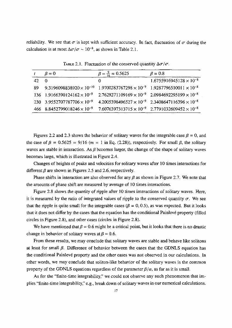
reliability. We see that c is kept with suMcient accuracy.
calculation is at most Ao'lo' •- 1O-8, as shown in Table 2.1 .
In fact, fluctuation of a during the
TABLE 2.1. F]uctuation of the conserved quantity Ao-la.
t 6=O P= & = O.5625 6= O.8
42
89
136
230
466
o93196098838920 Å~ 10-iO
1.9166390124162 Å~ 1O-9
3.9552707787706 Å~ 10-9
8.845279901 8246 Å~ 1O-9
o1 .9700283767298 Å~ 1 O-9
2,762927l 109169 Å~ 1O-9
4.2005398496527 Å~ 1O-9
7,6076397313715 Å~ 1O-9
1.6755916945128 Å~ 1O-8
1.928779651OOI1 Å~ 1O-8
2.0984692295199 Å~ 1O-8
2.3408647116396 Å~ 1O-8
2.7791032609452 Å~ 1O-8
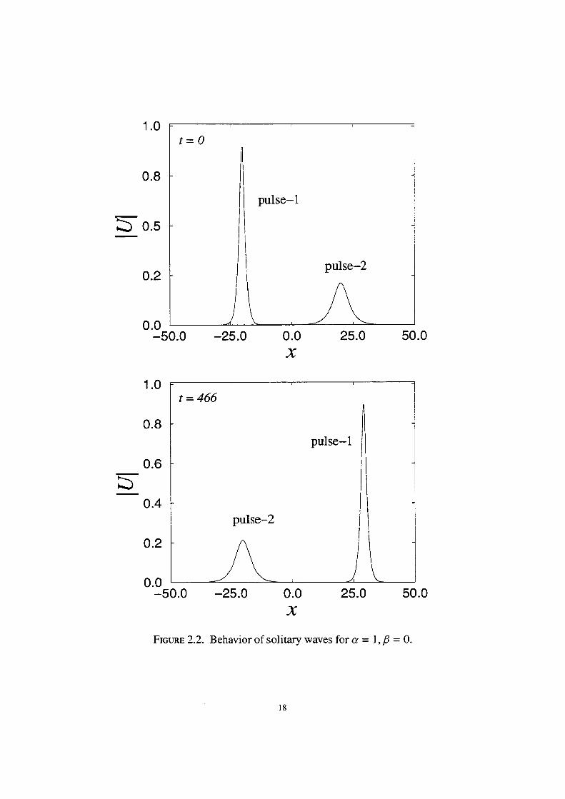
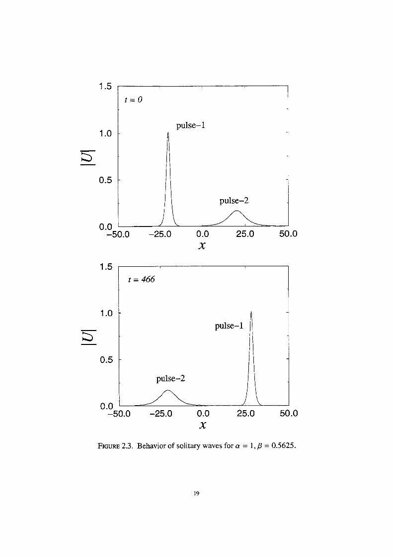
Figures 2.2 and 2.3 shows the behavior of solitary waves for the integrable case 13 = O, and
the case of6 = O.5625 = 9116 (m = 1 in Eq. (2.28)), respectively. For small 6, the solitary
waves are stable in interaction. As6 becomes larger, the change of the shape of solitary waves
becomes 1arge, which is illustrated in Figure 2.4.
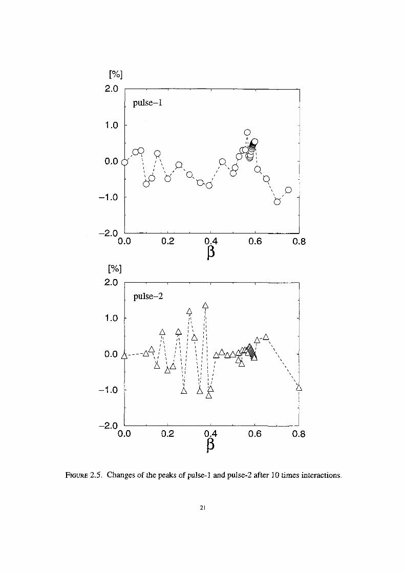
Changes of heights ofpeaks and velocities for solitary waves after 1O times interactions for
differentl3 are shown in Figures 2.5 and 2.6, respectively.
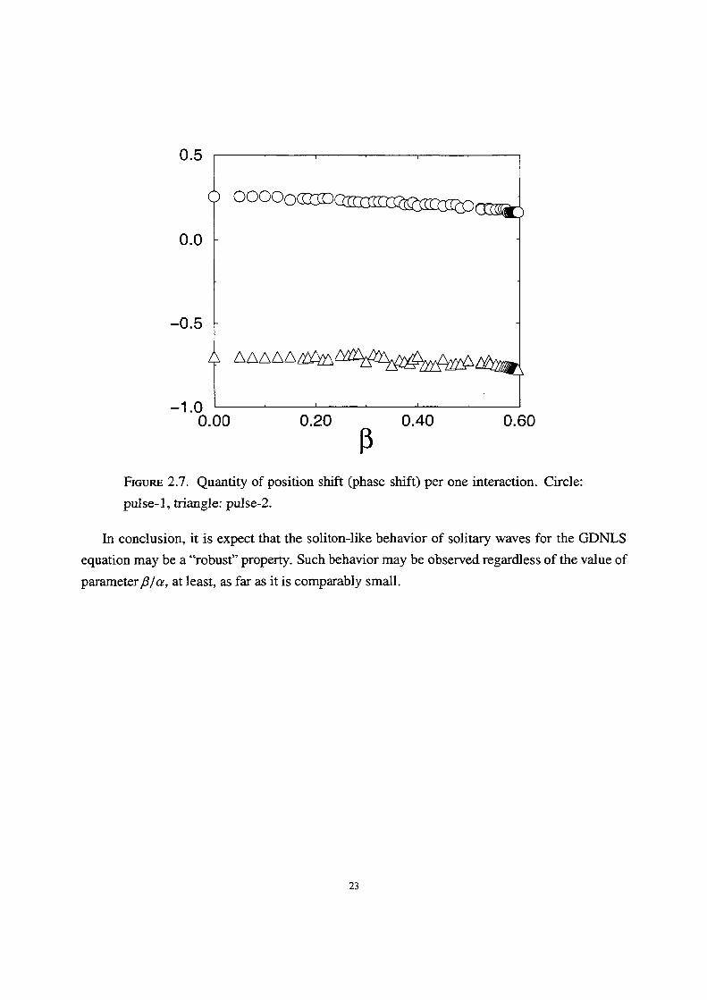
Phase shifts in interaction are a]so observed for any I3 as shown in Figure 2.7. We note that
the amounts of phase shift are measured by average of 1O times interactions.
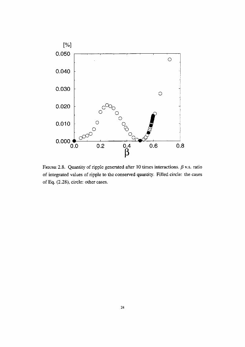
Figure 2.8 shows the quantity of ripple after 1O times interactions of soJitary waves. Here,
it is measured by the ratio of integrated values of ripple to the conserved quantity a. We see
that the ripple is quite small for the integrable cases (t3 = O, O.5), as was expected. But it looks
that it does not differ by the cases that the equation has the conditional Painleve property (filled
circles in Figure 2.8), and other cases (circles in Figure 2.8).
We have mentioned thatP = O.6 might be a critical point, but it ]ooks that there is no drastic
change in behavior of solitary waves at5 = O.6.
From these results, we may conclude that solitary waves are stable and behave like solitons
at least for small P. Difference of behavior between the cases that the GDNLS equation has
the conditional Painleve property and the other cases was not observed in our calculations. In
other words, we may conclude that soliton-like behavior of the solitary waves is the common
property of the GDNLS equations regardless ofthe parameterfila, as far as it is small.
As for the "finite-time integrability;' we could not observe any such phenomenon that im-
plies "finite-time integrability;' e.g., break down of solitary waves in our numerical calculations.
17
1 .0
O.8
:S O.5
O.2
o.o
1 .0
O.8
O.6 )
O.4
O.2
o.o
t=o
pulse-1
pulse--2
-50.0 -25.0 o.o
X25.0 50.0
t=466
pulse-2
pulse-1
-50.0
FIGuRE 2.2.
-25.0 O.O 25.0 X
Behavior of solitary waves for a = 1
18
50.0
,6=O.
1 .5
1 .0
)
O.5
o.o
t=0
pulse-1
pulse-2
-- 5O.O -25.0 o.o.JJC
25.0 50.0
1.5
1 .0
)
O.5
o.o
t= 466
pulse-2
pulse-1
-50.0 -25.0 o.o.]c
25.0 50.0
FIGuRE 2.3. Behavior of solitary waves for a = 1 ,P = O.5625.
19

1 .5
1 .0
ii)
O.5
o.o
t=o
pulse-- 1
pulse-2
-50.0 -25.0 o.o
X25.0 50.0
1 .5
1 .0
l)
O.5
OdO
t= 466
pulse--2
pulse-1
t
-50.0 -25.0 o.o
X25.0 50.0
FIGuRE 2.4. Behavior of solitary waves for a = 1 , 6 = O.8.
20
[o/o]
2.0
1 .0
o.o
-- 1.0
-2.0
[o/o]
2.0
1.0
o.o
-1.0
-2.0
pulse-1
/(Pl Ql
iN x it x !Q
IN te No•i Q 'oo
9, ss'
ON/ N8 O.cl)
NxIQU
o.o O.2 O.4p
O.6 O.8
pulse-2 4, ZIiX ll tl il rl 11 ll t
"'-
zsA,,ixr'fti Nizi tst,, z{l`' X ivii' 2ilivgi,; ;, AAn{{{i?flii 4N'ANNx,,,,
II lt l ,t A Lk
NN
Nx
NN
O.O O.2 O.4 O.6 O.8 6
FiGuRE 2.5. Changes of the peaks of pulse-1 and pulse-2 after 1O times interactions,
21
>-'--oo-o>
1 .0
o.o
-1.0
-2.0
-3.0
d
A(xAAAAajAAAZ2Xzy>,ly>z!njl,AA
FIGuRE
pulse-l
O.O O.2 O.4 O.6 O.8 p
2.6. Velocities of solitary waves after 10 times interactions. Circle:
, triangle: pulse-2. initial velocities are O.1 and -2.0, respectively.
5. Concluding remarks
ln this chapter, we have considered the GDNLS equation (2.I), and constructed a traveling
wave solution (2.19) which is valid for any values of parameters. Motivated by the explicit
form of the solution, we have applied the Painleve test to the GDNLS equation, and shown that
it possesses the Painlev6 property in strict sense only for the known integrable cases, and the
conditional Painlev6 property for the cases of Eq. (2.36).
Numerical results imply that the traveling wave solution is stable in the interaction and
behaves like a soliton for smal1 P, regardless of the possession of the Painleve property. Re-
markable difference in the behavior of solitary waves between inte.qrable and non-integrable
cases was not observed, except that quantity of ripple generated by the interaction of solitary
waves was small for integrable cases, as was expected.
As for the behavior of solitary waves for larger6, we could observe the change of shapes of
solitary waves by the interaction. However, it looks that it is stiIl insuMcient to conclude that
the solitary waves are not stable. Further theoretical analysis on stability may be necessary.
22
O.5
o.o
-O.5
-1.0
oooooascanrtwwn
AAAMzt>Cv>,zly21Z)>4 pt
o.oo O.20 O.40 O.60p
FiGuRE 2.7. Quantity of position shift (phase shift) per one interaction.
pulse-1 , triangle: pulse-2.
Circle:
in conclusion, it is expect that the soliton-like behavior of solitary waves for the GDNLS
equation may be a "robust" property. Such behavior may be observed regardless of the value of
parameter6/a, at least, as far as it is comparably small.
23
[o/o]
O.050
O.040
O.030
O.020
O.OlO
o.ooo
oCoo o
o ocgpo
J
oo
o ((i]'
oo
o
o
o.o 02 O.46
O.6 O.8
FiGuRE 2.8. Quantity of ripp]e generated after 1O times interactions. I3 v.s. ratio
of integrated values of ripple to the conserved quantity. Filled circle: the cases
of Eq. (2.28), circle: other cases.
24
CHAPTER 3
An Extension of the Steffensen Iteration and Its Computationa}
Complexity
1. introduction
ln this chapter, we consider iteration methods for finding a root of a single non}inear equa-
tion f(x) = O.
The Newton method is based on a first order approximation of the function f(x). The
sequence given by it generical]y converges locally and quadratically to a root a of f(x). There
have been many attempts to accelerate the Newton method. For example, some methods are
designed based on a higher order approximation (cf. [20]), on a composition of the Newton
iteration [66], on a Pade approximation [64, 16], on a modification of f(x) in such a way that
the convergence rate is increased [22, M], and so on.
The Steffensen method [72] is an iteration method which is applied to a nonlinear equation
of the forrn x = ip(x). It also has the second order convergence rate, and its iteration function
Åë(x) has no derivative of ip(x). The Steffensen method can be regarded as a discrete version
of the Newton method. There are so many extensions for the Newton method, however, a few
extension for the Steffensen method. The aim of this chapter is to develop a new iteration
method of the Steffensen type having a higher order convergence rate.
in Section 2, we consider a relationship of the Newton method and the Steffensen method.
In Section 3, we note that the Steffensen iteration function O(x) is congruent with the Aitken
transform [5]. In Section 4, we introduce the k-th Shanks transform [70] which is a natural
extension of the Aitken transform. When k = 1, the Shanks transform is reduced to the Aitken
transform. in Section 5, we propose an extension of the Steffensen method in terms of the
k-th Shanks transform. In Section 6, it is proved that the extension has the (k + 1)-th order
convergence rate provided that ip'(a) : O,Å}1. wnen Åë(a) = O, the iterated sequence has the
(k + 2)2k-i-th order convergence rate. In Section 7, some numerical examples are gi'ven which
demonstrate the eMcacy of the extended Steffensen iteration. For a special case of the Kepler
equation, it is shown that the numbers of mappings are actua]ly decreased by the extended
Steffensen iteration. In Section 8, we state the remarks of this chapter.
as
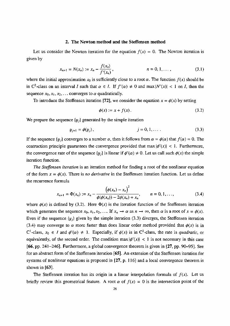
2. The Newton method and the Steffensen method
Let us consider the Newton iteration for the equation f(x) = O. The Newton iteration is
gi'ven by
f(Xn) , n= O, 1,..., (3.1) Xn+1 = N(Xn) := Xn '- f'(Xn)
where the initial approximation xo is suMciently close to a root a. The function f(x) should be
in C2-class on an interval I such that a E I. If f'(a) : O and max IN'(x)l < 1 on I, then the
sequence xo,xi,x2,... converges to a quadratically.
To introduce the Steffensen iteration [72], we consider the equation x = ip(x) by setting
ip(x) := x+f(x). (3.2)We prepare the sequence {yj} generated by the simple iteration
yJ•.i=ip(yj), j= O, 1,.... (3.3)If the sequence {yj} converges to a number a, then it follows from a = ip(a) that f(a) = O. The
contraction principle guarantees the convergence provided that max Iip'(x)I < 1. Furthermore,
the convergence rate of the sequence {yj} is linear if ip'(a) 4 O. Let us cal1 such Åë(x) the simple
iteration function.
77te Steffensen iteration is an iteration method for finding a root of the nonlinear equation
of the form x = Åë(x). There is no derivative in the Steffensen iteration function. Let us define
the recurrence formula
(ip(Xn) -' xn)2
Xn'1 = O(Xn) := Xn - Åë(ip(x,)) -2Åë(x.)+ x.' n= O' 1''''' (3'4)
where ip(x) is defined by (3.2). Here O(x) is the iteration function of the Steffensen iteration
which generates the sequence xo,xi,x2, .. .. If x. - a as n - oo, then a is a root ofx = Åë(x).
Even if the sequence {yJ•} given by the simple iteration (3.3) diverges, the Steffensen iteration
(3.4) may converge to a more faster than does linear order method provided that Åë(x) is in
Ci-class, xo E I and ip'(a) it 1. Especially, if Åë(x) is in C2-class, the rate is quadratic, or
equivalently, of the second order. The condition max lip'(x)l < 1 is not necessary in this case
[66, pp. 241-246]. Furthermore, a global convergence theorem is gi'ven in [27, pp. 90-95]. See
for an abstract form of the Steffensen iteration [65]. An extension of the Steffensen iteration for
systems of nonlinear equations is proposed in [27, p. 1 16] and a local convergence theorem is
shown in [63].
The Steffensen iteration has its origin in a linear interpolation formula of f(x). Let us
briefly review this geometrical feature. A root a of f(x) = O is the intersection point of the
26
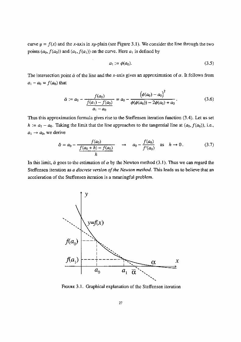
curve y = f(x) and the x-axis in xy-p]ain (see Figure 3.1). We consider the line through the two
points (ao, f(ao)) and (ai ,f(ai)) on the curve. Here ai is defined by
ai := ip(ao). (35)The intersection point tr of the line and the x-axis gives an approximation of a. It follows from
ai -- ao = f(ao) that
- f(ao) (ip(ao)-ao)2 a:="o -' f(a,)-f(ao) ="o-ip(Åë(ao)) -- 2Åë(ao)+ao' (3'6)
al -ao
Thus this approximation formula gives rise to the Steffensen iteration function (3.4). Let us set
h := ai - ao, Taking the limit that the line approaches to the tangential line at (ao, f(ao)), i.e.,
ai - ao, we derive
tr=ao- f(.,+f80-)f(.,) -> ao'ff,((a.O,)) as h->o. (3.7)
h
In this limit, tr goes to the estimation of a by the Newton method (3.1 ). Thus we can regard the
Steffensen iteration as a discrete version ofthe Newton method. This leads us to believe that an
acceleration of the Steffensen iteration is a meaningful problem.
N
y
sNNN
NNN
y=rtx)
f(ao)
NNNN
NNv---s
1N.N1NNlSNNN
rtai) 1"-T"""-I
NsN
1
NN-N
ocÅ~N Å~Å~
FiGuRE 3.1 . Graphical explanation of the Steffensen iteration
27
3. The Steffensen method and the Aitken transform
Let us introduce the Aitken transform [5]. It is a sequence transform to accelerate the
convergence of a given sequence {yi}. The Aitken transform is given by
ijj=YJ '- y,iYt"5i,.Y', )i y,, J= o, 1,2,.... (3.s)
If the sequence {yj} converges to a finite limit y., then the sequence {ijJ•} converges to the same
limit y. faster than {yj}. ln general (cf. [10, pp. I-2]), we consider some sequences {S ,•}, {Tj},
anda sequence transform such that A:Sj . Tj. If the sequences {Sj} and {Tj} converge to the
same ]imit a and satisfy the condition
Tj-a ]•tM. s,-.=O• (3.9)
then the sequence transform A is called sequence convergence accelerator.
The Steffensen iteration function O(x.) is equivalent to the Aitken transform of the three
numbers x., ip(x.) and ip(ip(x.)). Narnely, we have
(Yi ' yo)2 Yo = Xn, Yi =Åë(Xn), Y2 = ip(ip(Xn)) (3•10) O(xn) = ijo := Yo - y2 -2yl + yo '
for each n = O, 1,,... It should be noted that the sequence {ijJ•} accelerated by the Aitken
transform is different from the sequence {x.} generated by the Steffensen iteration (3.4). We
can find that xn+i = ijo and xn+2 : iji in general, even if xn = yo. In order to use the Aitken
acceleration, we must prepare the whole sequence {yj}. Moreover, if the convergence rate of
{yj} is linear, then the convergence rate of {gJ•} is so (cf. [6]). The Aitken acce]eration only
guarantees that the sequence {9]•} converges faster than {yi•} does in general. This property is in
sharp contrast to the Steffensen iteration.
4. The Shanks transform and the s-algorithm
77te k-th Shanks transform [70] is a natural extension of the Aitken transform.
by a ratio of Hankel determinants of 2k + l numbers y]•, . . . , yj+2k by
AÅí!' J'=O,1,2,.... ek(yJ') := BÅípt
28
It is defined
(3.1 1)
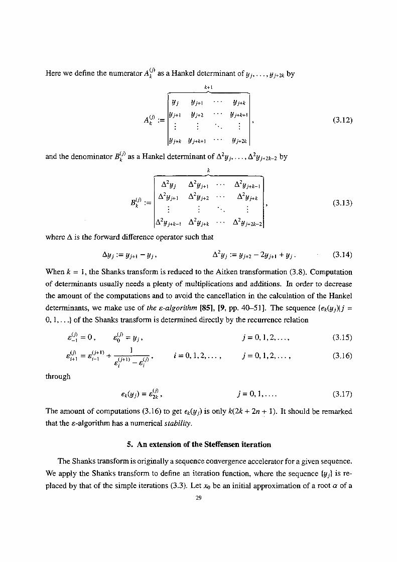
Here we define the numerator AÅí!) as a Hankel deterininant of yj, . . . , yj+2k- by
k+1 ij Yj Yj+1 ''' YJ'+k
AÅí.J) :. Yj.+1 YJI+2 ':' YJ+.k+1, (3.12)
---- -t -- Yi+k Yj+k+1 ''' Yj+2kt
and the denominator BÅí.J) as a Hankel deteminant of A2yj,,..,A2yj+2k-2 by
k A2yJ- A2yj.i ••• A2y]•+kmi
A2yj.i A2yj.2 ••• A2yJ'+k BÅí.J) := . .. ., (3.13) - --- - -i- A2yj.k-i A2yj.k ••' A2yi'+2kr-2
where A is the forward difference operator such that
Ayj := yj+i -- yj, A2yj := yj+2-2y]•+i+yj. (3.14)
When k = l, the Shanks transform is reduced to the Aitken transformation (3.8). Computation
of determinants usually needs a plenty of mukiplications and additions. In order te decrease
the amount of the computations and to avoid the cancellation in the calculation of the Hankel
deterrninants, we make use of the s-algorithm [85], [9, pp. 40-51]. The sequence {ek(yj)IJ' "--'
O, l, . . .} of the Shanks transform is determined directly by the recurrence relation
E(-J? =O, 68])=yj, j= O, 1, 2, ..., (3.15) 1 Sf•l), =6f•l ')+ .{j.,)-.{,), i--•-- O, 1,2,..., J' = O, 1,2,..., (3.16)
ltthrough
ek (yj)=sS',?, i= O, 1,.... (3.1 7)
The amount ofcomputations (3.16) to get ek(y,•) is only k(2k + 2n Å} l). It should be remarked
that the s-algorithm has a numerical stability.
5. An extension of the Steffensen iteration
The Shanks transform is originally a sequence convergence accelerator for a given sequence.
We apply the Shanks transform to define an iteration function, where the sequence {yJ•} is re-
placed by that of the simple iterations (3.3). Let xo be an initiai approximation of a root a of a
29
nonlinear equation x = ip(x). For a fixed natural number k, we introduce the following iteration
function
Ak(Xn) Xn+i=Ok(Xn) := Bk(x,), n=O, 1,2,•••• (3.18)
Here we define Ak(x) and Bk(x) as
ÅëO(X) ipi(X) ''' Åëk(X)
ipi(X) ip2(X) ''' Åëk+i(X) Ak(x):=. . .. , (3.19) -- -- -- ipk(X) ipk+i(X) ''' ip2k(X)
62Åëo(x) 62ipi(x) ••• 62ipk-i(x)
62Åëi(x) 62ip2(x) ••• 62ipk(x)
Bk(x) :=. . .. . (3.20) - - i- 62Åëk-i(x) 62ipk(x) ••• 62ip2k--2(x)
The number x.+i becomes a new staning value for the next iteration. Here ipj•(x) and 62Åëj(x) are
compositions of the simple iteration function Åë(x) and their linear combinations defined by
j -'N'A-"A ipo(x) := x, ipj(x) := Åë(ip(•••ip(x)•••)), j= 1,2,3,...,2k, (3.21)
62Åëj(x) := ipj.2(x) -- 2ip,•.i(x) + ip,-(x), J' = O, l,..., 2k-2, (3.22)
respectively. If a denominator in the forrnula (3.18) happens to be zero, we set xn+i = xn.
Especially, Oi(x) isjust the Steffensen iteration function (3.4). Let us cal] (3.18) the extended
Steffensen iteration.
6. Convergence rate of the extended Steffensen iteration
We now consider the convergence rate of the extended Steffensen iteration (3.I 8). The main
results in this chapter are as follows.
THEoREM 3.1 . lf ip(x) is in Ck'i-class and Åë'(a) ;E O, Å}1, then the extended Steffensen iter-
ation has the (k + 1)-th order convergence rate. Namely, lxn+i - al s Clx. --- alk'i for some
constant C.
Proof. Without loss of generality we can assume a = O where a is a root of x = ip(x). We
shal1 compute the leading term of the Taylor expansion of the iteration function Åëk(x) around
x=O. 30
Let us perform the fol}owing operations to the determinants Ak(x), Bk(x). Seuing
dnÅë(o) , n= 1, 2, ..., (3.23) Cn := dxn
we first subtract the i-th row multiplied by ci from the (i + 1)-th row for i = 1,2, . . .. On the
next step, we subtract the i-th row multiplied by ci2 from the (i + 1)-th row for i = 2, 3, . . .. We
do the similar operations recursively. Then we can express the Hankel determinants (3.19) and
(3.20) as
ai,o(x) al,1(x) ••i al.k(x)
a2,i(x) a2,2(x) ••• a2.k+ 1 (X) Ak(x)= . . . . , -t- ak+IS-(X) ak+IS•+1(X) ''' ak+1,2k(X)
b,,o(x) bi.i(x) ••• bi,k-i(x)
b2,,(x) b,.,(x) ••• bzk(x) Bk(x)= . . . . . bk,k-i(x) bks-(x) ••• bk,2k--2(x)
Here we define a.,j(x) and b..j(x) as
ai,j(x) := Åëj(x), j= O, l,...,2k, a.+1,j(x) := am,j(x) -- clMa..j-1(x), m=1,2,...,k, 1' -- m,m+1,...,2k,
bi,j(x) := 62ipj(x), j--- O, l,.,.,2k-2, bm+1,j(X) : : bm,j(X) -- CIM bm,j-1(X) , M = 1, 2, ...,k- 1 , j= m,m+ l,..., 2k 'rr 2
First we consider the Steffensen case where k = 1 .
al,1(x) = cl x+ gc2f+••• , al,o(x) = x,
a2.i (x) = Sc2f +•••, a2,2(x) = Sci 2c2 x2 +••• .
Obviously, we have
Ai (x) = Sc, (c, - 1)c, x3 +... ,
Bi (x) = (ci -l)2x+ g(ci2 + ci - 2)c2 x2 +••• .
It follows from the condition ci : O, 1 that Oi(x) =
convergence.
31
(3.24)
(3.25)
(3.26)
(3.27)
(3.28)
(329)
By the Taylor expansion of Ai (x) we see
(3.30)
(3.31)
(3.32)
(3.33)
O(x2) as x . O. This proves the quadratic
Next we show that Åëk(x) = O(xk"i) for any natural number k. The functions am,]•(x) take the
form
m-1 a.,i(x) = ip](.)c)+2X3fM)ip,e,(x), 13{,M) := (-l)t Z ciPi"P2" 'Pt . (3.34)
i=l O<pl<•••<Pi<MThis can be checked by using the recurrence relation (3.27). We consider the n-th order deriva-
tive of the composition Åëj(x) = Åë,•-i(ip(x)), which is expressed as
dndip.',(X)=ll.i],(dr/i}(ip,,l:.2:::.z;c..s(qi,•••,q,)dqd'e(,X)•••dqd'liij(.")) (3.3s)
forn= 1,2,.... Here C(gi,...,g,) are unique constants. We define the constants C(qi,q2,...)
for qi E {O, 1,2,...},i= 1,2,..., as follows:
(i) C(qi,...,q,-,O) = C(qi,..•,qj),
(ii) C(...,qi,...,gj,...) =Oif qi < qj,
(iii) C(l) = 1, r C(qi,•••, q.) = ZKC(qi, •• •, qi-i, qi - 1, gi+i, •• •, q.) if gr > O,
i=1where K is the number of the non-negative integers having the sarne values as gi - 1 in the set
{ql,•••,qi-1,qi -- 1,gi+1,...,qr}, namely,
K:= #{n :gi-1inE {qi,..•,gi-i,gi -- 1,qi+i,•••,qr}}•
By use of (3.35) and C(l,..., 1) = 1, we write ipS.")(O) := d"Åëj(O)ldx" as
n-1 ipS") (O) = ci"ipS."-), (O) + Z 7(.n)Åë Sl), (O) , 7;"> := Z C(qi, • • •, qr) Cq, Cq2 ' ' ' Cq. •
r=1 gl+"'+gr=n qlZ--Zgr>OUsing (3.34) and (3.37), we see for ain")i(O) : : dna.,,•(O)!dx" as fo]lows:
m-1 ahl',(O) = gbY'(O) + Z,BS•M'{bSZ',(O)
i--1 = c,nipSe-),(o) + :., •)tsn)Åëir-),(o) + th.,' ,f3(,m) (c,ngbSn-),-,(o) + ii.Il, •>,gn)gbS"2,-,(o))
= c,n (Åëin-),(o) + :., x3S•m>ipSn-),.,(o)) + :., 7s-n) (ipir-), (o) + il.Iiii., /3Em)ÅëSr-),.,(o))
n-1 = c,nah"),.-, (o) + Z 7S")aX)j-,(O) ,
r=1
32
(3.36)
(3.37)
(3.38)
We insert (3.38) into the n-th order derivative of (3.27) to derive
n-1 aShnl,,j (o) = (c,n - c, M)a[h"?j-, (o) +2 7iÅín)aÅíh'),.., (o) . (3.3g)
r=1 Assume that a.,j(x) = O(xM), name]y,
ah"?,.(O)=O, for n<m, (3.40) ah"?,.(O):O, for n=m. (3.41)The right hand side of (3.39) is equal to O for n s m. While ainM.',1)(O) is not equal to O when
ci : O, 1. Then it follows that
ah"l,,,(O)=O, for n<m+1, (3.42) ah"l,,j(O):O, for n=m+l. (3.43)
This implies that a.+i,j(x) = O(xM'i). By induction we find that a.,j(x) = O(xM) for any natural
number m. Therefore, the Taylor expansion of a.,j(x) is given by
a.,,•(x) =ahny)(O) xM +-••. (3.44)
On the other hand, we can easily find that
bm,j=a.,j+2-2a.,j+i+am,i, m=1,2,...,k, j=m-1,m,...,2k-2 (3.45)
from the definition (3.29). Then we obtain
bh"),.(o)=o, for n<m, (3.46)
' bh"]j(O)=(ciM--1)2asc).(O):O, for n=m (3.47)
from (3.38), (3.44), (3.45) and the condition ci 4 Å}l . Hence we have
b.,j(Jc)=bhny).(O) xM +••• (3.48)
for any natural number m.
Finally we consider the deteminants Ak(x) and Bk(x). Let S. be the set of permutations
a=( ,O•, ii, III Z•.1', )ofn-items. By virtue of(3.24), (3.25), (3.44) and (3.48), we see
Ak(X) = Z sgn o'•ai,ioazi+i, •••ak+i.k.ik =Lx(k+i>(k+2)i2 +•.. , (3.4g)
aESk+1 Bk(x) = Z sgn a•bi.iob2,i.i, ••tbk,k-i.i,-, =MM'(k'i)/2 +••• . (3.so)
aESk
33
Here we define constant L as
a:16(o) aS',l(o) •-• ai12.(O)
aS?l(O) aS?l(o) ••• aS22..,(o) L= . .. ., (3.51) - --- -v -- aÅíS.",i2.(o) aÅíS,'4`2..,(o) ••• aÅíS.';'3,(O)
andMas bii,B(o) bgi,l(o) ••• bii2-,(o)
bZl(o) b9(o) ••• bS?2.(o)
M= . . .. (3.52) . t --- blSl2.-,(O) bÅíSjl(O) ••t bÅíSll.-,(o)
This means that Ok(x) = O(xk"i ). The extended Steffensen iteration defined by the k-th Shanks
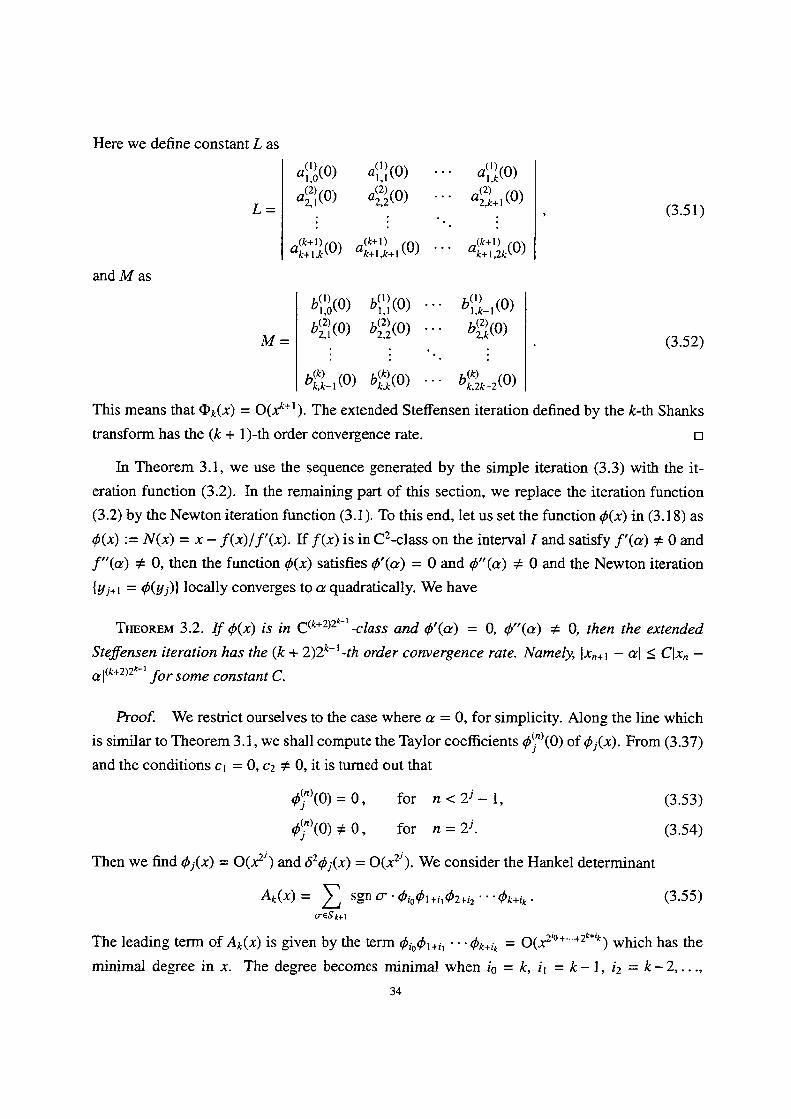
transforrn has the (k+1)-th order convergence rate. m in Theorem 3.l, we use the sequence generated by the simple iteration (3.3) with the it-
eration function (3.2). ln the remaining part of this section, we replace the iteration function
(3.2) by the Newton iteration function (3.1 ). To this end, Iet us set the function ip(x) in (3.1 8) as
ip(x) := N(x) = x - f(x)lf'(x). if f(x) is in C2-class on the interval I and satisfy f'(a) # O and
f"(a) : O, then the function ip(x) satisfies ip'(a) = O and Åë"(a) : O and the Newton iteration
{yj+i = ip(yj)} locally converges to a quadratical]y. We have
THEoREM 3.2. if ip(x) is in C(k'2)2"-'-class and ip'(af) = O, ip"(a) : O, then the extended
Steffensen iteration has the (k + 2)2k-i-th order convergence rate. Namely, lxn+i - al S CIxn -
al(k'2)2k"'i for some constant C.
Proof. We restrict ourselves to the case where a = O, for simplicity. Along the ]ine which
is similar to Theorem 3.I , we shal1 compute the Taylor coeMcients ipS.")(O) of ipj(x). From (3.37)
and the conditions ci = O, c2 : O, it is turned out that
ÅëS.")(O)=O, for n<2'-l, (3.53) ÅëS."'(O):O, for n=2j. (3.s4)Then we find ipj(x) = O(x2') and 62Åëj(x) = O(x2'). We consider the Hankel determinant
Ak(x)= 21 sgnc•ipi,Åëi+i,ip2+i..•••ipk+i,• (3.55)
aESk+1The leading term of Ak(x) is given by the term Åëi,ipi.i, • • • ipk.i, = O(x2lo"'"2k'ik) which has the
minimal degree in x. The degree becomes minimal when io = k, ii =k-1, i2 =k-2,•••,
34
ik =O. It follows that Ak(x) = O(x(k'i)2k). Similarly, Bk(x) = O(.xk'2k-i). Consequently, we see
Åëk(x) =o(x(k'2)2k'i) which completes the proof of Theorem 3.2. u
In the book of Ostrowski [66, p. 252] a composition of the Newton iterations is formulated
which has third-order convergence. The iteration in Theorem 3.2 with k = l provides third-
order convergence. The extended Steffensen iteration in this case is also a composition of the
Newton iterations, however, it is rather different from that in [66].
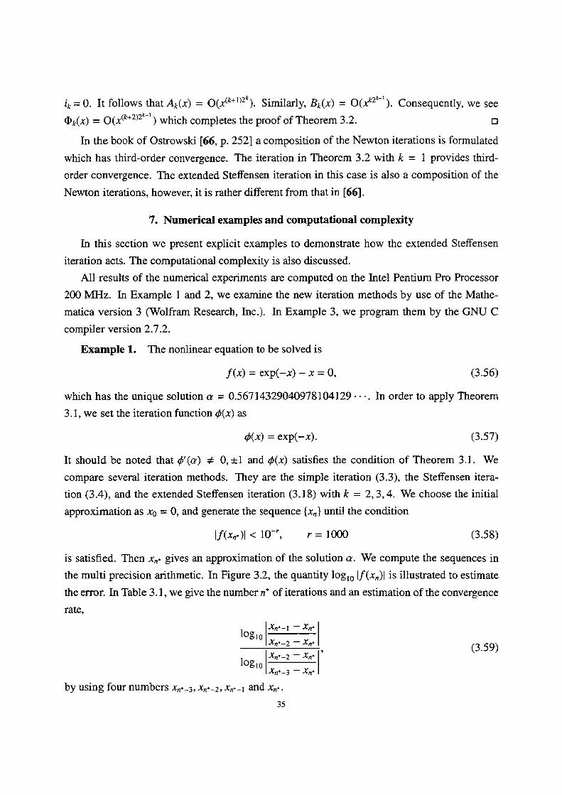
7. Numerical examples and computational complexity
in this section we present explicit examples to demonstrate how the extended Steffensen
iteration acts. The computational complexity is also discussed.
All results of the numerical experiments are computed on the lntel Pentium Pro Processor
200 MHz. ln Example 1 and 2, we examine the new iteration methods by use of the Mathe-
matica version 3 (Wolfram Research, lnc.), In Examp]e 3, we program them by the GNU C
compiler version 2.7.2.
Example 1. The nonlinear equation to be solved is
f(x)=exp(-x) -x= O, (3 .56)which has the unique solution a = O.56714329040978104129•••. In order to apply Theorem
3.I, we set the iteration function ip(x) as
Åë(x)=exp(--x). (3.57)It should be noted that ip'(a) # O,Å}1 and Åë(x) satisfies the condition of Theorem 3.1. We
compare several iteration methods. They are the simple iteration (3.3), the Steffensen itera-
tion (3.4), and the extended Steffensen iteration (3.18) with k = 2, 3,4. We choose the initial
approximation as xo = O, and generate the sequence {x.} until the condition '
lf(x.• )1 <10-", r= 10oo (3.58)is satisfied. Then x.. gives an approximation of the solution a. We compute the sequences in
the multi precision arithmetic. In Figure 3.2, the quantity logio lf(x.)i is illustrated to estimate
the error. in Table 3. 1 , we give the number n' of iterations and an estimation of the convergence
rate,
Xn'-1 ' Xn' logio Xn'-2 d Xn' , (359) Xn'-2 - Xn' logio Xn'-3 ' Xn'by using four numbers xn,-3, xn.-2, xn.-i and xni•
35
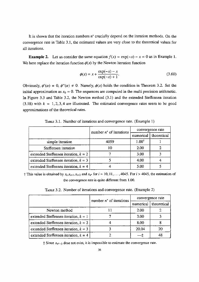
It is shown that the iteration numbers n' crucially depend on the iteration methods. On the
convergence rate in Table 3.1, the estimated values are very close to the theoretical values for
all iterations.
Example 2. Let us consider the sarne equation f(x) = exp(-x) -- x = O as in Example 1.
We here replace the iteration function ip(x) by the Newton iteration function
exp(-x) - x . (3.60) ip(x) = x + exp(-x) + 1
Obviously, Åë'(a) = O, ip"(a) : O. Namely, Åë(x) holds the condition in Theorem 3.2. Set the
initial approximation as xo = O. The sequences are compuied in the multi precision arithmetic.
In Figure 3.3 and Table 3.2, the Newton method (3.1) and the extended Steffensen iteration
(3.l8) with k = 1,2,3,4 are illustrated. The estimated convergence rates seem to be good
approximations of the theoretical rates.
TABLE 3.I. Number of iterations and convergence rate. (Example 1)
numbern'ofiterationsconvergencerate
numerical theoretical
simpleiteration 4059 1.0ot 1
Steffenseniteration 10 2.00 2
extendedSteffenseniteration,k=2 7 3.00 3
extendedSteffenseniteration,k=3 5 4.oo 4
extendedSteffenseniteration,k=4 4 5.00 5
t This value is obtained by xi,xi+i,xi+2 and xn. for i = 1O, 1 l, . . . ,4045. For i > 4045, the estimation of
the convergence rate is quite different from 1 .00.
TABLE 3.2. Number of iterations and convergence rate. (Example 2)
numbern'ofiterationsconvergencerate
numerical theoretical
Newtonmethod ll 2.00 2
extendedSteffenseniteration,k=1 7 3.00 3
extendedSteffenseniteration,k=2 4 8.00 8
extendedSteffenseniteration,k=3 3 20.04 20
extendedSteffenseniteration,k=4 2 -$ 48
i Since xn.-3 dose not exist, it is impossible to estimate the convergence rate.
36
o
-200
-400A-sRsv
9bO -600o-
-800
-10oo
hNNNNN
NNN
N s N N s t s s l s s , 1 1 l i s
O 5 10 15 20 itr.# n
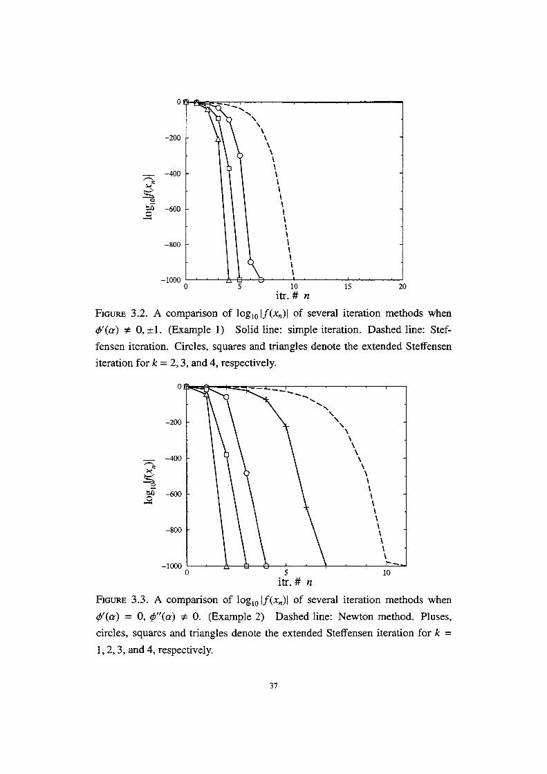
FiGuRE 3.2. A comparison of logiolf(x.)l of several iteration methods when
Åë'(a) # O,Å}1. (Example 1) Solid line: simple iteration. Dashed line: Stef-
fensen iteration. Circles, squares and triangles denote the extended Steffensen
iteration for k = 2, 3, and 4, respectively.
o
-2oo
400ArRx 9bD -6ooo-
-800
-1ooO
-'k. k.- NN.--.
NNxNN
NN
NNNN
NNNN
N s N N N N s s N s s
o 5 itr. # n
of logiolf(x.)l of several
(Example2) Dashedline:
b
10
FJGuRE 3.3. A comparison iteration methods whenip'(a) = O, ip"(a) # O. Newton method. Pluses,circles, squares and trianales denote the extended Steffensen iteration for k =
1, 2, 3, and 4, respectively.
37
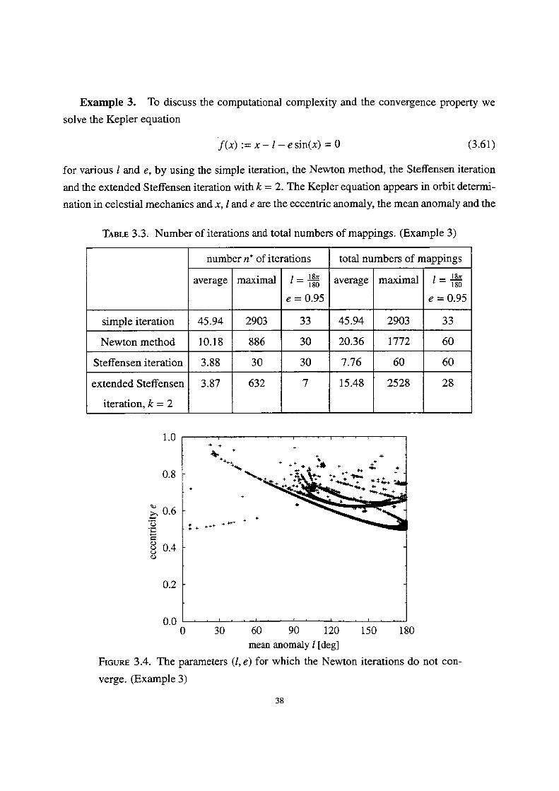
Example 3. To discuss the computational complexity and the convergence property we
solve the Kepler equation
f(x) :=x-- l-esin(x) =O (3.61)
for various l and e, by using the simple iteration, the Newton method, the Steffensen iteration
and the extended Steffensen iteration with k = 2. The Kepler equation appears in orbit determid-
nation in celestial mechanics and x, l and e are the eccentric anomaly, the mean anomaly and the
TABLE 3.3. Number of iterations and total numbers of mappings. (Exarnple 3)
numbern'ofiterations totalnumbersofmappings
average maximal 18nl='i'gT,e=O.95
average maximal l..l.g8gg
e=O.95
simp}eiteration 45.94 2903 33 45.94 2903 33
Newtonmethod 10.18 886 30 20.36 l772 60
Steffenseniteration 3.88 30 30 7.76 60 60
extendedSteffensen
iteration,k=2
3.87 632 7 l5.48 2528 28
1.0
O.8
Y O.6'6'8'
g O.4
O.2
o.o
+
t'
++$+ ++++ N
+ -++++
+
+ .# ++ +.." .sN.. .+.es X..- " +'s'+' + .
++
- + ++ --- + +- - +i".:•,,/1 •l. l.:'"ir'?
+,
+
.
o 30
FiGuRE 3.4. The parameters (l, e
verge. (Example 3)
60 90 120 150 180mean anomaly l [deg]
) for which the Newton iterations do not con-
38
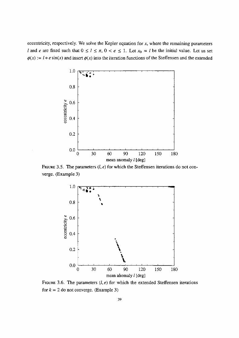
eccentricity, respectively. We solve the Kepler equation for x, where the remaining parameters
l and e are fixed such that O S l s z, O < e s 1. Let xo = lbe the initial value. Let us set
ip(x) := l+ e sin(x) and insert Åë(x) into the iteration functions of the Steffensen and the extended
1.0
O.8
Y O.6'6:t
88 O.4o
O.2
o.o
n +- ++t"+
o 30
FiGuRE 3.5 . lhe parameters (l, e
verge. (Example 3)
60 90 120 150 180mean anomaly l [deg]
) for which the Steffensen iterations do not con-
1.0
O.8
Y O.6'-o
•:.
88 O.4O
O.2
o.o
+t ):"
+-
s,
.,x
'x
o
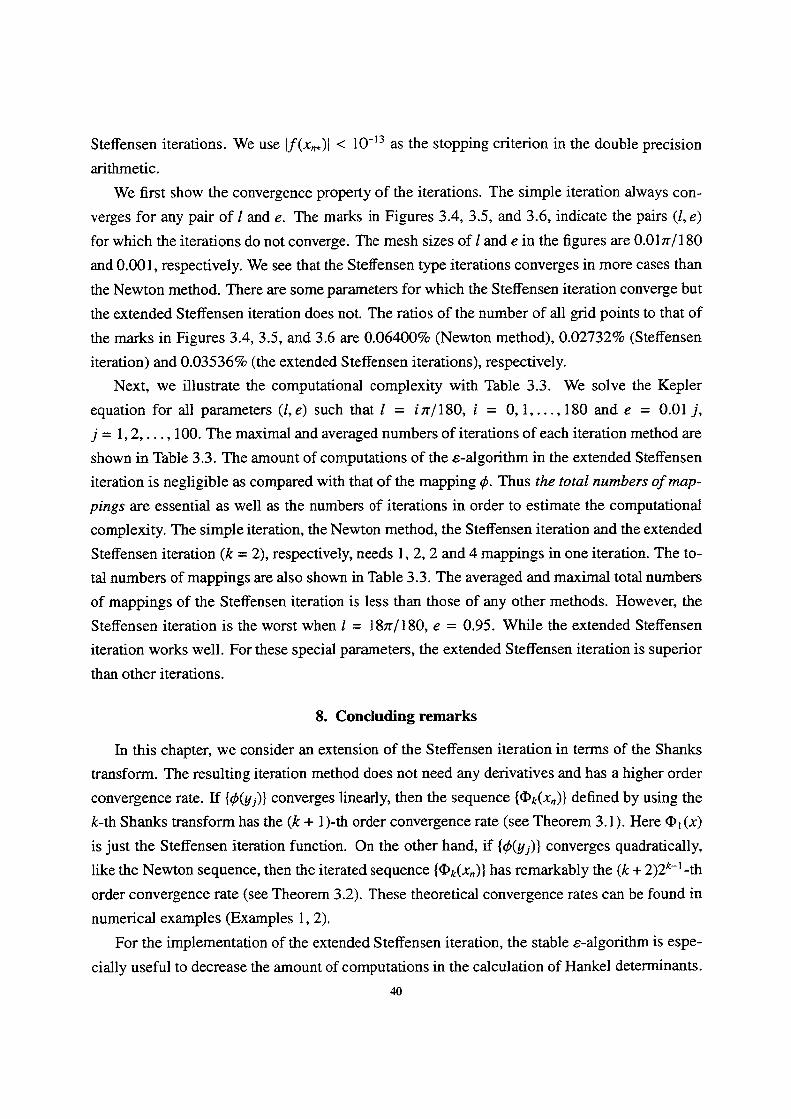
FiGuRE 3.6. The parameters (l,e
for k = 2 do not converge.
30 60 90 120 150 180 mean ahomaiy l [deg]
) for which the extended Steffensen iterations
(Example 3)
39
Steffensen iterations. We use lf(x..)1 < 10-i3 as the stopping criterion in the double precision
arithmetic.
We first show the convergence property of the iterations. The simple iteration always con-
verges for any pair ofland e. The marks in Figures 3.4, 3.5, and 3.6, indicate the pairs (l, e)
for which the iterations do not converge. The mesh sizes of l and e in the figures are O.Olnl1 80
and O.OO1, respectively. We see that the Steffensen type iterations converges in more cases than
the Newton method. There are some pararneters for which the Steffensen iteration converge but
the extended Steffensen iteration does not. The ratios of the number of all grid points to that of
the marks in Figures 3.4, 3.5, and 3.6 are O.064009o (Newton method), O.027329o (Steffensen
iteration) and O.035369o (the extended Steffensen iterations), respectively.
Next, we illustrate the computational complexity with Table 3.3. We solve the Kepler
equation for all parameters (l, e) such that l = irr1180, i = O, l,...,180 and e = O.Ol J',
j' -- 1, 2, . . . , 1OO. The maximal and averaged numbers of iterations ofeach iteration method are
shown in Table 3.3. The amount of computations of the E-algorithm in the extended Steffensen
iteration is negligible as compared with that of the mapping ip. Thus the total numbers ofmap-
pings are essential as well as the numbers of iterations in order to estimate the computational
complexity. The simple iteration, the Newton method, the Steffensen iteration and the extended
Steffensen iteration (k = 2), respectively, needs 1, 2, 2 and 4 mappings in one iteration. The to-
tal numbers of mappings are also shown in Table 3.3. The averaged and maximal total numbers
of mappings of the Steffensen iteration is less than those of any other methods. However, the
Steffensen iteration is the worst when l = 18nll80, e = O.95. While the extended Steffensen
iteration works well. For these special parameters, the extended Steffensen iteration is superior
than other iterations.
8. Concluding remarks
in this chapter, we consider an extension of the Steffensen iteration in terms of the Shanks
transform. The resulting iteration method does not need any derivatives and has a higher order
convergence rate. lf {Åë(yj)} converges linearly, then the sequence {Ok(x.)} defined by using the
k-th Shanks transform has the (k + 1)-th order convergence rate (see Theorem 3.1). Here Åëi (x)
is just the Steffensen iteration function. On the other hand, if {ip(yJ•)} converges quadratically,
like the Newton sequence, then the iterated sequence {Ok(x.)} has remarkably the (k + 2)2k-t -th
order convergence rate (see Theorem 3.2). These theoretical convergence rates can be found in
numerical examples (Examples 1, 2),
For the implementation of the extended Steffensen iteration, the stable s-algorithm is espe-
cially useful to decrease the amount of computations in the calcu]ation of Hankel determinants.
co
Consequently, the numbers of mappings take a major part of the computational complexity. It
is shown (Example 3) that the extended Steffensen iteration with k = 2 has the minimal num-
bers of mappings in a special case of the Kepler equation. Moreover, the extended Steffensen
iteration converges for more cases of parameters than the Newton method.
After the completion of this research the authors are told the references [10], [48] by Pro-
fessor N. Osada, which considers a generalized Steffensen iteration without any discussion on
computational complexity. The idea in [48] is essentially the same as that in this thesis, however,
there is no explicit numerical examples and no comparison to other iteration methods.
41
CHAPTER 4
Determinantal Solutions for Solvab]e Chaotic Systems and Iteration
Methods Having Higher Order Convergence Rates
1. introduction
The singularity confinement (SC) is a useful integrability criterion for discrete nonlinear
dynamical systems [25]. The discrete Painlev6 equations and many discrete soliton equations
pass the SC test. However the SC test is not suMcient to identify integrability. In the literature
[28], Hietarinta and Viallet presented a discrete dynamical system which passes the SC test but
possesses a numerically chaotic property. Then they proposed a more sensitive integrability test
[28, 8] using the algebraic entropy. The algebraic entropy is defined by the logarithmic average
of a .qrowth of degrees of iterations. Both test are similar to each, and the algebraic entropy test
is a more precise criterion than the SC test.
Many of good numerical algorithms are deeply connected to the nonlinear integrab]e sys-
tems. For example, the recurrence relation of the qd-algorithm, which is used for calculating
a continued fraction, is equivalent to the discrete time Toda equation. And the recurrence rela-
tion of the s-algorithm [85], which is a sequence convergence accelerator, is equivaient to the
discrete potential KdV equation. From these results, one may conjecture that good numerical
algorithms can be regared as integrable dynamical systems. indeed, many of linearly convergent
algorithms such as eigenvalue algorithms and sequence accelerators pass the SC type criteria
(cf. [68]), and they are proved to be equivalent to soliton equations. However, the algorithms
having higher order convergence rates, which give irreversible dynamical systems, do not pass
the SC type criteria. The techniques in the nonlinear integrable systems cannot be directly
adapted to them.
The arithmetic-harmonic mean (AHM) algorithm [62] is an irreversible system having an
explicit solution, however does not pass the SC type criteria. According to the setting of initial
conditions, it behaves as an algorithm having the second order convergence rate, or as a solvable
chaotic system. in this chapter, we investigate such discrete dynamical systems and obtain their
determinantal solutions. We deal with the Ulam-von Neumann (UvN) system [77] which is
a solvable chaotic system, and with the discrete dynamical systems derived from the Newton
method, an extension of the Newton method, the Steffensen method [72], and the extended
42
Steffensen method proposed in Chapter 3, which are iteration methods having higher order
convergence rates.
In Section 2, we show the trigonometric solutions for the AHM algorithm and the UvN
system in terms of addition formulas. Moreover we show the hierarchy of the UvN system.
The AHM algorithm is equivalent to the Newton method for a quadratic equation. In Section
3, we introduce the Newton method and the Nourein method [64, 16] which is an extension of
the Newton method. Applying these methods to a quadratic equation, we present the hierarchy
of the Newton type iterations. In Section 4, we give addition formulas of the determinants of
certain tridiagonal matrices. In Section 5, we show determinantal solutions for the discrete Ric-
cati equation. ln Section 6, we obtain determinantal solutions for the hierarchy of the Newton
type iterations. In Section 7, determinantal solutions for the hierarchy of the UvN system are
derived. In Section 8, we obtain determinantal solutions for the hierarchy of the Steffensen type
iterations. ln Section 9, we give some remarks.
2. Ttigonometric solutions for solvab}e chaos systems
ln this section, we introduce solvable chaotic systems which have trigonometric solutions.
We shai] show that these solutions are obtained in terms of some addition formulas.
Firstly, we consider the iteration
an+i = an;bn, bn+t = in a+t bbnn, n= O, 1, 2, •••, (4•1)
which is cal}ed the arithmetic-harmonic mean (AHM) algorithm [62]. The AHM algorithm has
the following solutions. For the case ao > bo > O, we have
a.=Ni coth (2"ai), b.=Ni tanh (2"ai). (4.2)
For the case ao > O, bo < O, we have
a. =N2 cot (2"a2), b. = --N2 tan (2"a2). (4.3)
Here the positive constants Ni, N2, ai and a2 are uniquely detemined by the initial values ao
and bo. The solutions (4.2) and (4.3) are derived from the double angle formulas of coth(x) and
cot(x),
2 coth(x)tanh(x) coth(x) + tanh(x) 2 , tanh(2x) = coth(.) +t..h(.), (4'4) coth(2x) =
2 cot(x) tan(x) cot(x) - tan(x) 2 , tan(2x)=cot(.) .-. ta.(.), (4'5) cot(2x) =
43
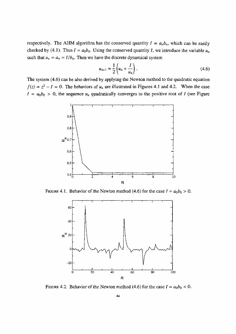
respectively. The AHM algorithm has the conserved quantity I = anbn, which can be easily
checked by (4.1). Thus I = aobo. Using the conserved quantity I, we introduce the variable u.
such that un = an = I/b.. Then we have the discrete dynamical system
un+i =S (un+ iifi )• (4.6)
The system (4.6) can be also derived by applying the Newton method to the quadratic equation
f(z) = z2 - I = O. The behaviors of u. are illustrated in Figures 4.1 and 4.2. When the case
I = aobo > O, the sequence u. quadratically converges to the positive root of I (see Figure
O.9
O.8
tsRo.7
FIGuRE 4. 1 .
O.6
O.5
O.4
n
Behavior of the Newton method (4.6) for the case I = aobo > O.
60
40
3R 2o
FIGuRE 4.2.
o
-20
O 20 40 60 80 100 n
Behavior of the Newton method (4.6) for the case I = a
op
obo < O.
4.1). Wlien the case I = aobo < O, it behaves as a solvable chaotic system (see Figure 4.2). Its
invariant measure is #(dx) = dxl(n(1 + x2)), and its Lyapunov exponent is log 2 (cf. [79]).
Next, we consider the solvable logistic map, or the Ulam-von Neumann (UvN) system [77],
O< uo <l, Un+l = 4Un(1 - Un), n= O, 1, 2, ... . (4.7)
A solution for (4.7) is obtained by
un = sin2(2"a3) , (4.8)
which is derived from the double angle formu]a of sin2(x),
sin2(2x) = 4 sin2(x)(1 - sin 2(x))' (4.9)
Here the constant cr3 is determined by the initial value uo. The invariant measure of the UvN
system is pt(dx) = dx/(iT VI((i-=IJ), and the Lyapunov exponent of it is log2 (cf. [79]). By
virtue of the n-tuple angle formulas of uigonometric functions, the higher order systems of the
UvN system are given by
uL2.), =4uÅí2)(1-uÅí2)), (4.10) ui3.)i =uÅí3)(3 -- 4uÅí3))2, (4.11) u2`.), =l6 uÅí4)(1 -uÅí`))(l -- 2uk4))2, (4.12)
uÅí5.), =uÅí5)(5 -4uS5)(5 -4uA5)))2, (4.13)
and so on (cf. [80]). The superscripts m of uSM) denote the order of the hierarchy. Their invariant
measures are all v(dx) = dxl(z VI(( i-:-JE5), and their Lyapunov exponents are respectively ]og m
form = 3,4,5,. ... Another generalization of the UvN system having Jacobi or Weierstrass
elliptic function solution is discussed in [78].
An aim of this chapter is to obtain determinantal solutions for the discrete dynamical sys-
tems (4.6), (4.7) and their hierarchies. The hierarchy of (4.6) is introduced in Section 3, and the
hierarchy of (4.7) already appear above.
3. The Newton method and the Nourein method
ln this section, we introduce the Newton method (cf. [13]) and an extension of the Newton
method for finding a root of an equation f(z) = O. Furthermore we present a hierarchy of
discrete dynamical systems gi'ven by the Newton type iterations.
45
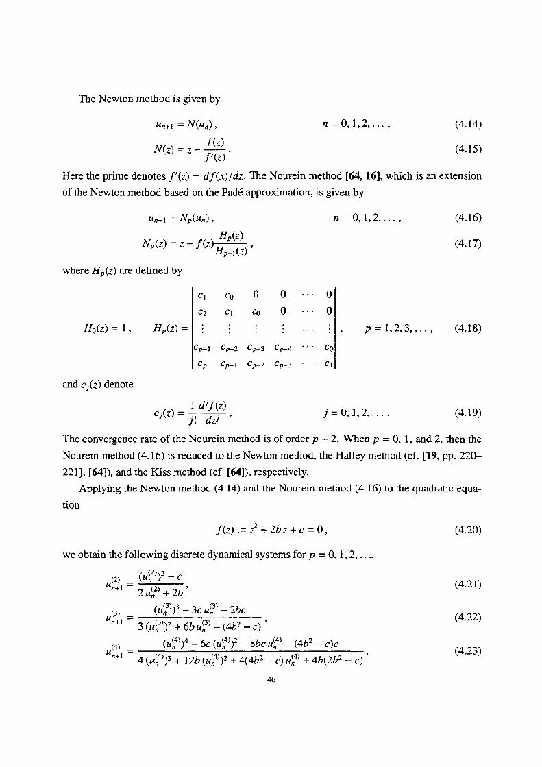
The Newton method is given by
Un+1 =N(Un), n= O, 1, 2, •.., N(z) =z-. f(Z). fr(z)
Here the prime denotes f'(z) = df(x)ldz. The Nourein method [64, 16],
of the Newton method based on the Pade approximation, is given by
Un+1=Np(Un), n= O, 1, 2, ..., Hp(z) N. (l) = Z - f(Z) H,., (z) '
where Hp(z) are defined by
Cl Co O O ••• O C2 Cl CO O ''' O Ho(z)=1, H.(z)= l i I I ••• i, p=1,2,3, Cp.1 Cp-2 Cp-3 Cp-4 ''' CO
Cp Cp.l Cp-2 Cp-3 ''' Cl
and cj(z) denote
cj(z) = -;.!d'df,SZ. ), ]' = o, i,2,....
The convergence rate of the Nourein method is of order p + 2. When p = O, 1,
Nourein method (4.16) is reduced to the Newton method,
221], [64]), and the Kiss method (cf. [64]), respectively.
tion
f(z) := z2 + 2bz+c=O,
we obtain the following discrete dynamical systems for p = O, l , 2, . . .,
(2) (uL2))2-c Un+i = 2uA2) + 2b '
(3) (uS3))3 - 3c uL3) - 2bc Un+i = 3 (uL3))2 + 6b ui3) + (4b2 - c) '
(4) - (uL`))` -- 6c (uS4))2 - 8bc uS`) - (4b2 - c)c U"'! 4(u:`))3 + 12b (uL`))2 + 4(4b2 - c) uÅí`) + 4b(2b2 - c) '
46
(4.I4)
(4.I5)
which is an extension
--- )
(4.16)
(4.17)
(4.18)
(4.19)
and 2, then the
the Hal]ey method (cf. [19, pp. 220-
Applying the Newton method (4.14) and the Nourein method (4.16) to the quadratic equa-
(4.20)
(4.21)
(4.22)
(4.23)
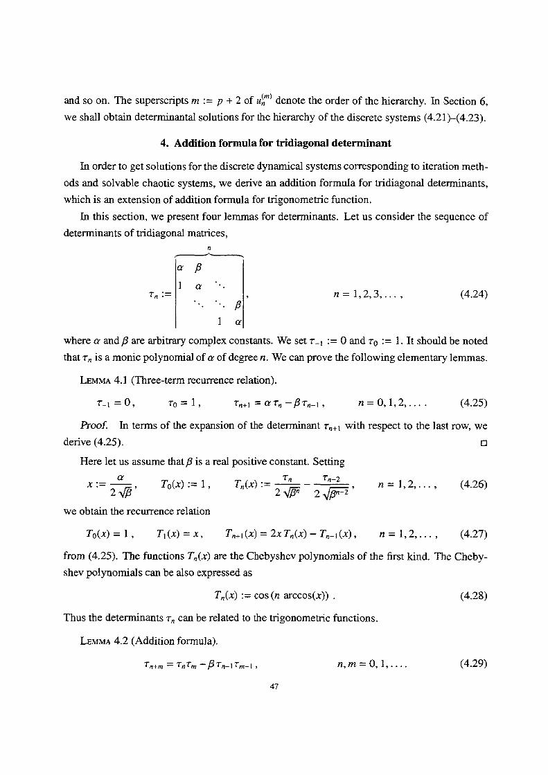
and so on. The superscripts m := p + 2 of uSM) denote the order of the hierarchy. In Section 6,
we shal1 obtain determinantal solutions for the hierarchy of the discrete systems (4.21 )-(4.23).
4. Additien formula for tridiagonal determinant
in order to get solutions for the discrete dynamical systems corresponding to iteration meth-
ods and solvable chaotic systems, we derive an addition formula for tridiagonal determinants,
which is an extension of addition formula for trigonometric function.
ln this section, we present four lemmias for determinants. Let us consider the sequence of
deteminants of uidiagonal matrices,
n - aP 1 a ''• Tn := , n= 1, 2, 3,..., (424) '•• '•• 6
la
where a and6 are arbitrary complex constants. We set T-i := O and To := l . It should be noted
that T. is a monic polynomial of a of degree n. We can prove the fol]owing elementary lemmas.
LEMMA 4.1 (Three-term recurrence relation).
Zi =O, To :l, Tn+i =aTn -J3 7'n-i, n= O, 1,2,.... (4.25)
Rroof. in terms of the expansion of the determinant T.+i vvith respect to the last row, we
Here let us assume that6 is a real positive constant. Setting
a Tn Tn-2 X:= 2f/3 , To (X) := i, Tn (X) := 2.vfxiiiE -2.,vc2i} Fi , n= i, 2, •••, (4•26)
we obtain the recurrence relation
To(X) =1, Tl (X) =X, Tn+i (X) = 2X Tn (X) - Tn-i (X), n= 1, 2,..., (4.27)
from (4.25). The functions T.(x) are the Chebyshev po]ynomials of the first kind. The Cheby-
shev polynomials can be also expressed as
T.(x) := cos(n arccos(x)). (4.28)Thus the deteminants 7, can be related to the trigonometric functions.
LEMMA 4.2 (Addition formula).
Tn+m = Tn Tm -J(3 Tn-ITm-1, n,M= O, 1,.... (4.29)
47
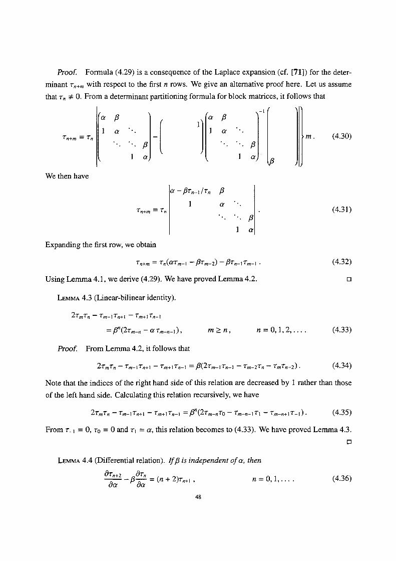
Rroof. Formula (4.29) is aconsequence of the Laplace expansion (cf. [71]) for the deter-
minant T.+. with respect to the first n rows. We give an altemative proof here. Let us assume
that T, : O. From a determinant panitioning formula for block matrices, it follows that
Tn+m= Tn
a61a'
•• 6
la
a6 a
.
.
1
6a
-1
m. (4.30)
We then have
a-J37'n-1ITn JEI
1 a ''• Tn+m=Tn • (4.31) '•• '•• p
la
Expanding the first row, we obtain
Tn+m = Tn (aTm-1 'h X3Tm-2) -jt3Tn-t 7'm-1 • (4.32)
Using Lemma 4.1, we derive (429). We have proved Lemma 4.2. z
LEMMA 4.3 (Linear-bilinear identity).
2Tm7'n - Tm-1Tn+l - Tm+lTn-t
=I3"(2Tm-n -aTm-n-i), m }) n, n= O, 1, 2,.... (4.33)
Proof. From Lemma 4.2, it follovvs that
27'mTn - Tm-ITn+1 - 7'm+ITn-1 = ](3(2Tm-ITn-l - Tm-21'n - TmTn-2)• (4•34)
Note that the indices of the right hand side of this relation are decreased by 1 rather than those
of the left hand side. Calculating this relation recursively, we have
27'mTn - Tm-ITn+1 - Tm+I Tn-i = X3" (2Tm-n7ro - 'rm-n-iTl - 1'm.n+IT-1). (4.35)
From ti = O, To = O and Ti = a, this relation becomes to (4.33). We have proved Lemma 4.3.
a
LEMMA 4.4 (Differential relation). lfJ(3 is independent ofa, then
OTn+2 0Tn =(n+2)Tn+i, n= O, l,.... (4.36) -6 Oa Oa
48
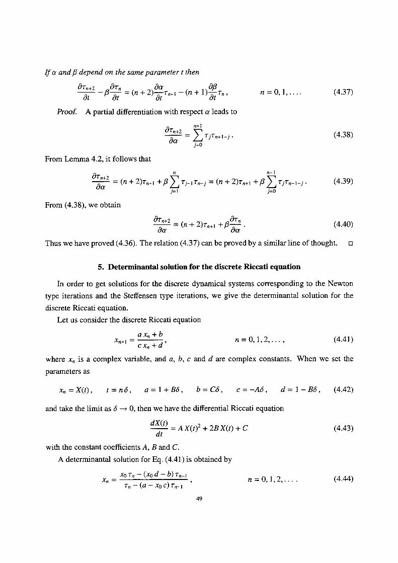
ifa and6 depend on the same parameter t then
0io'ni2 -ic3 0o7t'" :(n + 2)ili/llT.+i - (n+ i)l2/II Tn, n= O, i,•••• (4•37)
ProoL A partial differentiation with respect a leads to
n+1 OS"."2 =ÅíTjTn+i-JE• (4.38) J'--O
From Lemma 4.2, it follows that
n n-1 0a7'na'2 = (n + 2)Tn+1 +/3 2 7'j-ITn-j -'"b' (n + 2)7'n+1 +J(3 2 'rj7'n-l-j • (4•39)
j--o J'=1
From (4.38), we obtain
(i)Tn (OTn+2 . (4.40) = (n + 2)T.+1 +JEI Oa Oa
Thus we have proved (4.36). The relation (4.37) can be proved by a similar line of thought. u
5. Determinanta} solution for the discrete Riccati equation
in order to get solutions for the discrete dynamical systems corresponding to the Newton
type iterations and the Steffensen type iterations, we give the determinantal solution for the
discrete Riccati equation.
Let us consider the discrete Riccati equation
ax. +b , n= O, l, 2, ..., (4.41) Xn+l = cx. +d
where x. is a complex variable, and a, b, c and d are complex constants. When we set the
parameters as
x.=X(t), t=n6, a=1+B6, b=C6, c=-A6, d=1-B6, (4.42)and take the limit as 6 . 0, then we have the differential Riccati equation
dX(t) =A x(t)2+2B X(t) +C (4.43) dt
with the constant coeMcients A, B and C.
A determinantal solution for Eq. (4.41 ) is obtained by
x. ,. Xo 7'n'(XOd-b) Tn-1 , n=o, l,2,.... (4.44) 1'n - (a '- Xo C) Tn-1
49
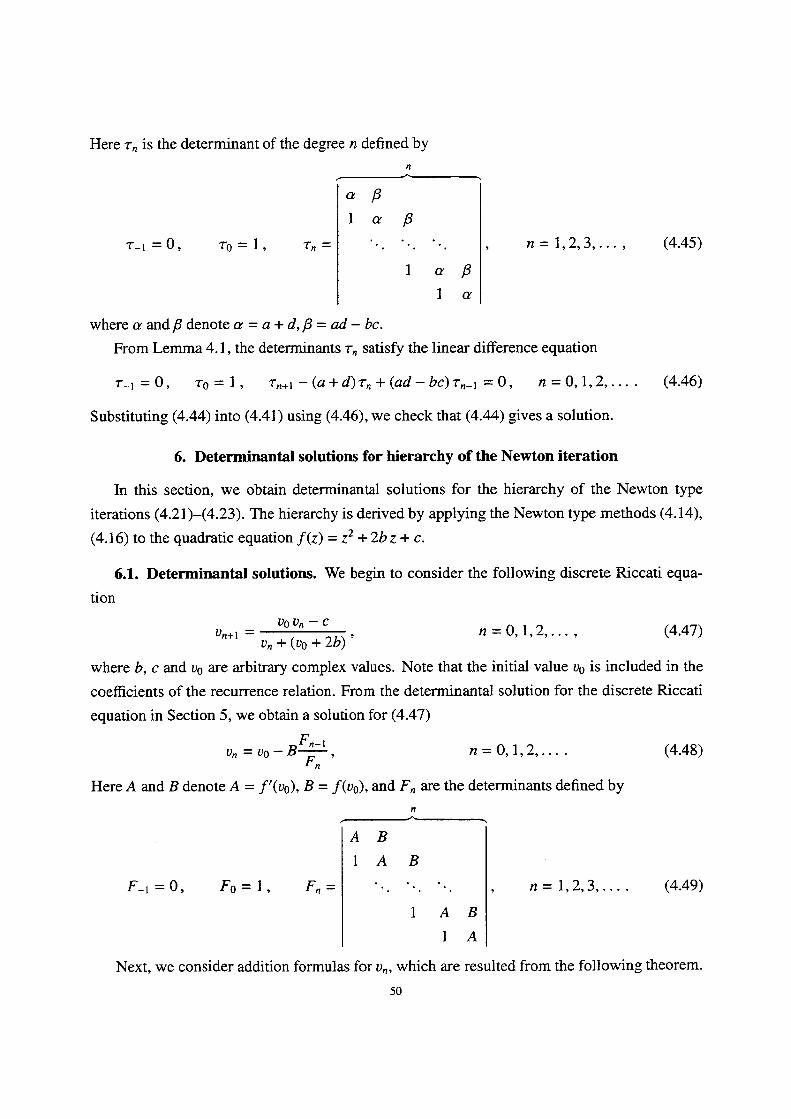
Here T, is the determinant of the degree n defined by
n - a6
la6 T-i =O, To =l, Tn = '•. '•. ••. , n= l, 2, 3, ..., 1 a6 la
where a and6 denote a = a+ d,6 = ad - bc.
From Lemma 4. 1 , the determinants T, satisfy the linear difference equation
7-i =O, To = 1, Tn+i - (a+d) 7'n + (ad- bc) T.-i = O, n= O, l, 2, ..
Substituting (4.44) into (4.41) using (4.46), we check that (4.44) gives a solution.
6. Determinanta1 solutions for hierarchy of the Newton iteration
In this section, we obtain deteminantal solutions for the hierarchy
iterations (4.21 )-(4.23).
(4.1 6) to the quadratic equation f(z) = z2 + 2b z + c.
6.1. Determinantal solutions.
tion
Vo Vn -- C Vn+1 = v. +(vo+2b) , n= O, 1, 2, ...,
where b, c and vo are arbitrary coinplex values. Note that the initial value vo
coeMcients of the recurrence relation.
equation in Section 5, we obtain a solution for (4.47)
v. =vo -BF"-i, n= o, 1, 2, .... FnHere A and B denote A = f'(vo), B = f(vo), and F. are the determinants defined by
n -"'--••--•- AB IAB
F-i=O, Fo=l, F.= '•. ••. '•. , n=1,2,3,... 1 AB IA
Next, we consider addition formulas for v.,
so
--
(4.45)
(4.46)
of the Newton type
The hierarchy is derived by applying the Newton type methods (4.14),
We begin to consider the following discrete Riccati equa-
(4.47)
is included in the
From the determinantal solution for the discrete Riccati
(4.48)
(4.49)
which are resulted from the following theorem.
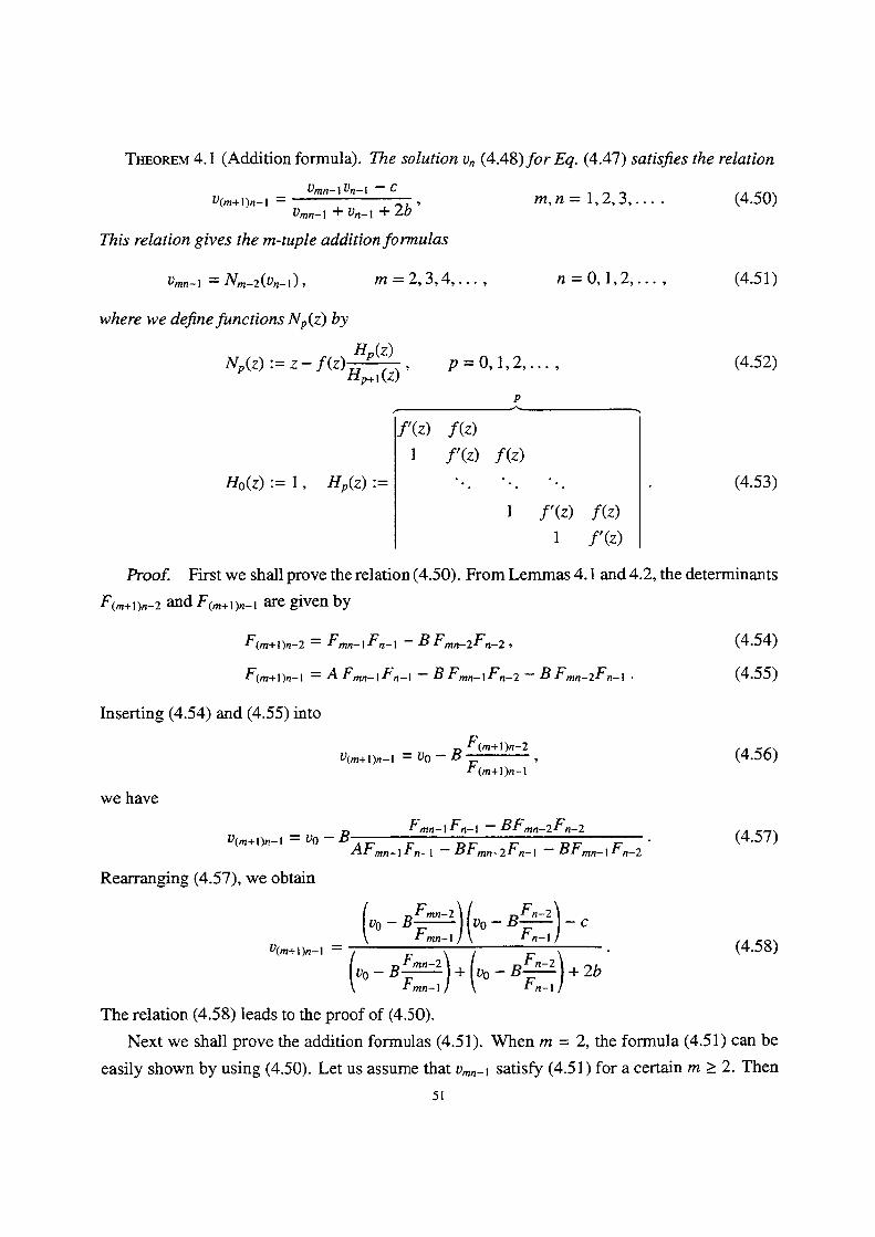
THEoREM 4.1 (Addition formula). The solution v. (4.48)for Eq. (4.47) satisJies the relation
Vmn-lVn-1 '- C V(M'1)"-1 = v..-1+v..1+2b' M,n= 1, 2, 3, '••• (4.50)
This relation gives the m-tuple additionformulas
Vmn-1 "IVm-2(Vn-1), M= 2, 3, 4, •••, n= O, 1, 2, ..., (451)
where we definefunctions Np(z) by
H. (z) , p= O, 1, 2, ..., (4.52) Np(z) := z- f(Z) Hp+i(Z)
p f'(z) f(z)
1 ft(z) f(Z)
Ho(z) :=1, Hp(z) := '•. '•. '•. . (4.53) l f'(z) f(z) 1 f'(z)
boof. First we shal1 prove the relation (4.50). From Lemmas 4.I and4.2, the determinants
F(m+i)n-2 and F(m+i)n-i are given by
F(m+l)n-2 = Fmn-I Fn-1 -BFmn-2Fn-2, (4.54) F(m+1)n-1 =A Fmn-IFn-1 -BFmn-IFn-2 -BFmn-2Fn-t • (455)
Inserting (4.54) and (4.55) into
F(m+1)n-2 , (4.56) V(m+t)n-i = vo 'B F(m+1)n-1
we have
Fmn-l Fn-i - BFmn-2Fn-2 . (457) v(m+i)n-i = vo -- B AFmn-1 Fn-1 -' BFmn-2Fn-1 - BFmn-1Fn-2
Rearrangi'ng (4.57), we obtain
fiil)--c llll:ll)(vo-B (vo -B
V(M'l)"'1 = (vo -Bill:n.f)+(vo -Bfll:i?)+ 2b (4 58)
The relation (4.58) leads to the proof of (4.50).
Next we shal1 prove the addition formulas (4.51). wnen m = 2, the formula (4.51) can be
easily shown by using (4.50). Let us assume that v..-i satisfy (4.51) for a certain m ) 2. Then
51
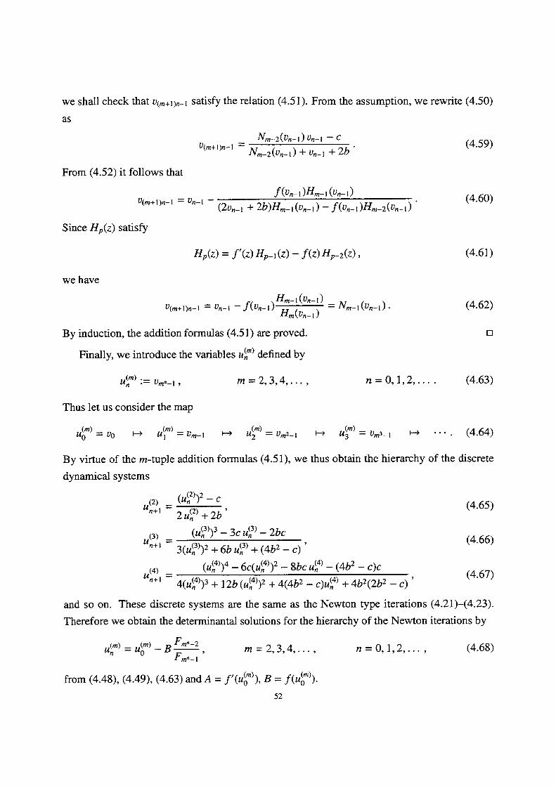
we shalI check that v(m+i).-i satisfy the relation (4.51). From the assumption, we rewrite (4.50)
as
Nm-2(Vn-1) Vn-1 - C V(M'i)n-i = N.-2(v.-i)+ v.-i +2b ' (4'59)
From (4.52) it follows that
f(Vn-1)Hm-i(Vn-i) V(M'i)"-i = Vn-i - (2v.-i + 2b)H.-i(v..i)-f(v,-i)H.-2(v.-i) ' (4'60)
Since H,(z) satisfy
Hp(z)=f'(z) H.-i (z)-f(z) H,-2(z), (4.61)
we have
Hm-1(Vn-1) =Nm-i(Vn-i)• (4.62) V(m+1)n-1 = Vn-1 -f(Vn-1) Hm(Vn-1)
By induction, the addition formulas (4.51) are proved. o Finally, we introduce the variables uSM) defined by
uÅíM) := v.n-i, m= 2, 3, 4,..., n= O, 1, 2,.... (4.63)
Thus let us consider the map
usm)=vo H uim)=v.-1 }-> usrn)=v.2-1 H ugm)=vm3.1 F•> •••. (4.64)
By virtue of the m-tuple addition formulas (4.51), we thus obtain the hierarchy of the discrete
dynamical systems
uL2.),=Il"ii/i))2.-i, (4•6s) (3) (uS3))3 - 3c uE3) - 2bc ""'i=3(uL3))2+6b .Åí3)+(4b2-,)' (4-66) (4) . (uL`))` -6c(ui`))2 - 8bc uS`) - (4b2 - c)c """ 4(uk`>)3 +12b (uS`))2 + 4(4b2 - c).s4) + 4b2(2b2 - ,) ' (4'67)
and so on. These discrete systems are the same as the Newton type iterations (4.21)-(4.23).
Therefore we obtain the determinantal solutions for the hierarchy of the Newton iterations by
uLm) =u6m) -B il; i":l, m= 2, 3, 4, ..., n= o, i, 2, ..., (4.6s)
from (4.48), (4.49), (4.63) andA = f'(u8M)), B = f(u6M').
52
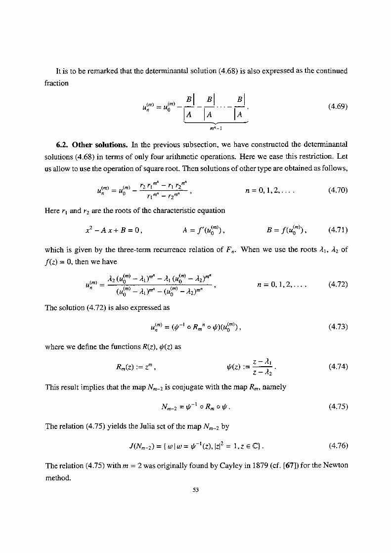
It is to be remarked that the deteminantal solution (4.68) is also expressed as the continued
fraction
BB B uLm)=u8M) -- --•••--. (4.6g) AA A - mn-1
6.2. 0ther solutions. in the previous subsection, we have constructed the determinantal
solutions (4.68) in terms of only four arithmetic operations. Here we ease this restriction. Let
us allow to use the operation of square root. Then solutions of other type are obtained as folloWs,
usm).usm)- r2 ;i ".'.n -- ;Ii2M", .. o, 1,2,.... (4.7o)
Here ri and r2 are the roots of the characteristic equation
x2 -Ax+B= o, A= f' (u8M)), B= f(u8M)), (4.71)
which is given by the three-term recurrence relation of F.. wnen we use the roots 1i, A2 of
f(z) = O, then we have
usm>-i2:2:lilii:.i:sÅí48.'-'i,i."nd, n-o,i,2,•••• (4•72)
The solution (4.72) is also expressed as
uSM) :(str-'oR."ogbf)(u8M)), (4.73)
where we define the functions R(z), V(z) as
z-11 R.(z) := zM, q(z) := z-A,• (4•74)
This result implies that the map N.-2 is conjugate with the map R., namely
N..2 =gbf-i oR.ou7. (4.75)
The relation (4.75) yields the Julia set of the map N.m2 by
J(N.-2) ={wl tv= ipf-i (z), lz12 = 1,zE (C}. (4.76)
The relation (4.75) with m = 2 was originally found by Cayley in 1 879 (cf. [67]) for the Newton
method.
53
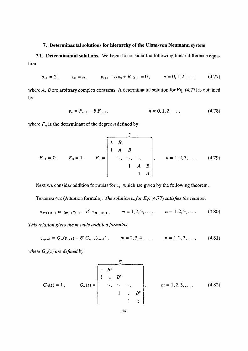
7. Determinanta} solutions for hierarchy of the Ulam-von Neumann system
7.1. Determinanta} solutions. We begin to consider the following Iinear difference equa-
tion
V-1 =2, Vo =A, Vn+1 '-AVn +BVn-1 =O, n= O, 1, 2, ..., (4.77)
where A, B are arbitrary complex constants. A detenninantal solution for Eq. (4.77) is obtained
by
Vn=Fn+1 -B Fn-1, n" O, 1, 2, •••, (4.78)
where F. is the determinant of the degree n defined by
n pt AB IAB F-i = O, Fo =1, Fn = ''. '•. ''. , n= l, 2, 3, .... (4.79) 1 AB IA
Next we consider addition formulas for v., which are given by the following theorem.
THEoREM 4.2 (Addition formula). The solution v, for Eq. (4.77) satisLfies the relation
V(m+i)n-i = Vmn-iVn-i - Bn V(m-i)n-i, m = l,2, 3,..., n = 1,2, 3,.... (4.80)
This retation gives the m-tupte additionformulas
vmn.i = Gm(vn-i)- B" Gm-2(vn.t), m= 2, 3, 4, ..., n= 1, 2, 3, ... , (4.81)
where G.(z) are deLtined by
m " z Bn
l z Bn
Go(z)=l, G.(z)= '•. '•. '•. , m=1,2,3,..., (4.82) 1 z Bn lz
54
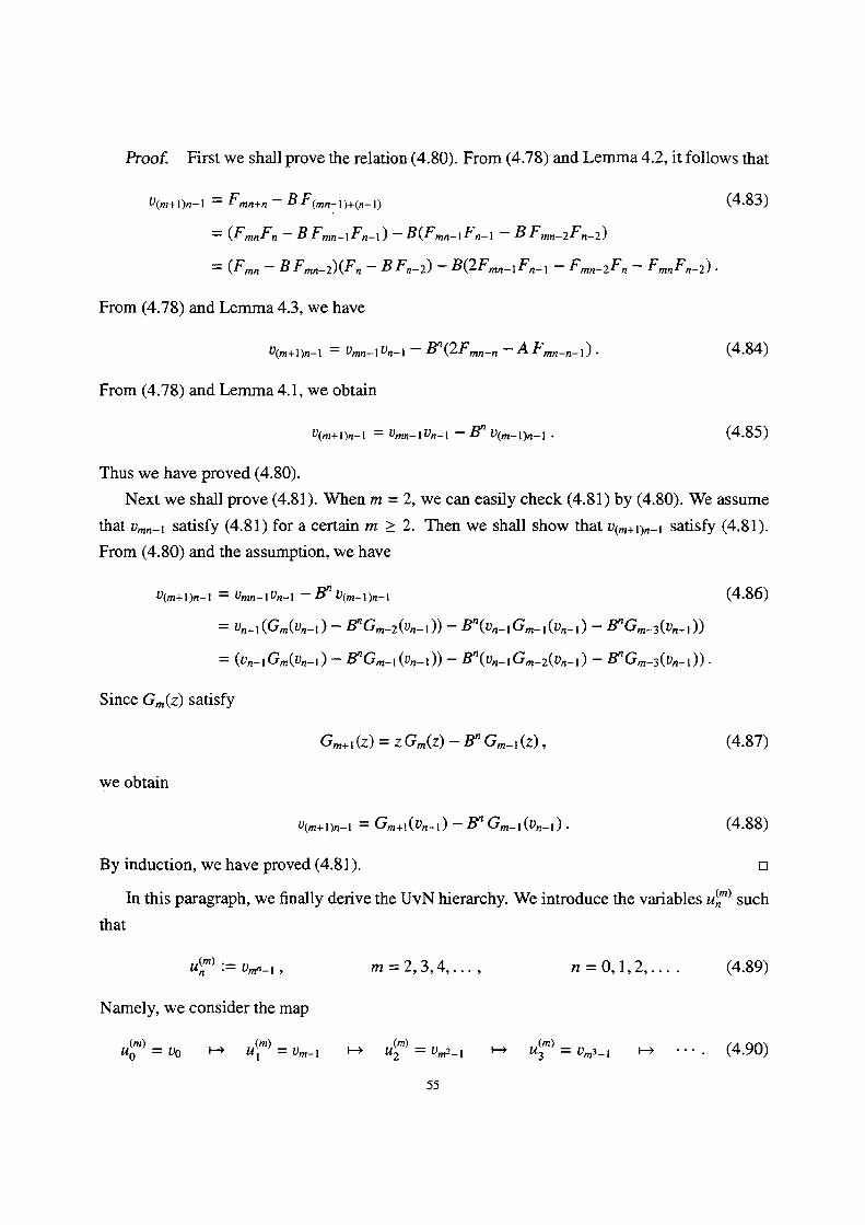
Rroof. First we shal1 prove the relation (4.80). From (4.78) and Lemma 4.2, it follows that
V(m+1)n-1=Fmn+n-BF(mn-b+(n-i) (4•83) = (FmnFn - B Fmn-i Fn-1 ) - B(jFmn-i Fn-1 - B Fmn-2Fn-2)
= (Fmn - B Fmn-2)(Fn - B Fn-2) - B(2Fmn-i Fn-i - Fmn-2Fn - FmnFn-2) •
From (4.78) and Lemma 4.3, we have
V(m+1)n-1 = Vmn-I Vn-l- Bn(2Fmn-n -A Fmn-n-1)• (4.84)
From (4.78) and Lemma 4.1, we obtain
V(m+1)n-1 = Vmn-I Vn-1 -B" V(m-1)n-1• (4.85)
Thus we have proved (4.80).
Next we shal1 prove (4.81). When m = 2, we can easily check (4.81) by (4.80). We assume
that v..-i satisfy (4.81) for a certain m 2 2. Then we shal1 show that v(.+i).-i satisfy (4,81).
From (4.80) and the assumption, we have
V(m+1)n-l=Vmn-IVn-1-Bn V(m-1)n-1 (4.86) = v.-i(G.(vn-i) - B"Gm-2(vn-i)) - Bn(vn-iGm-i(v.-i) - BnG.-3(v.-i))
= (vn-iGm(vn-i) - BnGm-i(vn-i)) •- B"(vn-iGm-2(vn-i) - BnG.-3(vn-i)) .
Since G.(z) satisfy
Gm+i (z) =zGm(z)-B" G.-i (z), (4.87)
we obtain
V(m+i)n-i = Gm+1(Vn-i)- B" Gm-i (Vn-i)• (4.88)
By induction, we have proved (4.81). m in this paragraph, vve finally derive the UvN hierarchy. We introduce the variables uLM) such
that
uSM) := v.n-i, m= 2, 3, 4,..., n= O, 1,2,.... (4.89)
Namely, we consider the map
u8M) = vo H uiM) = v.-i H u(2M) = v.2-i H ugM) = v.3.i H ••• . (4.90)
5S
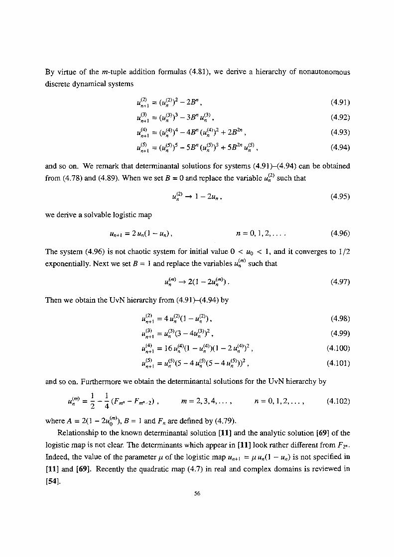
By virtue of the m-tuple addition formulas (4.81), we derive a hierarchy of nonautonomous
discrete dynamical systems
.Åí2.),=(uS2))2-2Bn, (4.91) uL3.), =(uS3) )3-3B" uS3), (4.g2) uÅí`.)i =(uÅí4) )4 -4Bn (uÅí4))2+2Bth, (4.93)
ui5.), =(uA5))5 •- sBn (uS5))3+sBin uS5), (4.g4)
and so on. We remark that determinantal solutions for systems (4.91)-(4.94) can be obtained
from (4.78) and (4.89). When we set B = O and replace the variable uÅí2) such that
uÅí2) ->l-2u., (4.95)
we derive a solvable logi' stic map
Un+1 =2Un(1 'Un), n" O, 1, 2, ..•• (4.96)
The system (4.96) is not chaotic system for initial value O < uo < 1, and it converges to 112
exponentially. Next we set B = 1 and replace the variables uÅíM) such that
uÅíM> --> 2(1-2uÅíM)). (4.97)
Then we obtain the UvN hierarchy from (4.9l )-(4.94) by
uS2.), =4uÅí2)(1-uS2>), (4.gs) uL3.), =uÅí3)(3-4uÅí3))2, (4.99) ui`.>, =i6 uS`)(1 -uS`))(i -2uL`))2, (4.loo)
uÅíllll), =uÅíl5)(5 -4uL5)(5 -4uÅí5)))2, (4.lol)
and so on. Funhermore we obtain the determinantal solutions for the UvN hierarchy by
uAM) =S-2(F.n - Fmn-2) , m= 2, 3, 4, •••, n= O, 1, 2, ..., (4.I02)
where A = 2(1 - 2u8M)), B = 1 and F. are defined by (4.79).
Relationship to the known determinantal solution [11] and the analytic solution [69] of the
logistic map is not clear. The determinants which appear in [11] look rather different from F2n.
Indeed, the value of the parameterp of the logi'stic map u.+i = uu.(l - u.) is not specified in
[11] and [69]. Recently the quadratic map (4.7) in real and complex domains is reviewed in
[54].
56
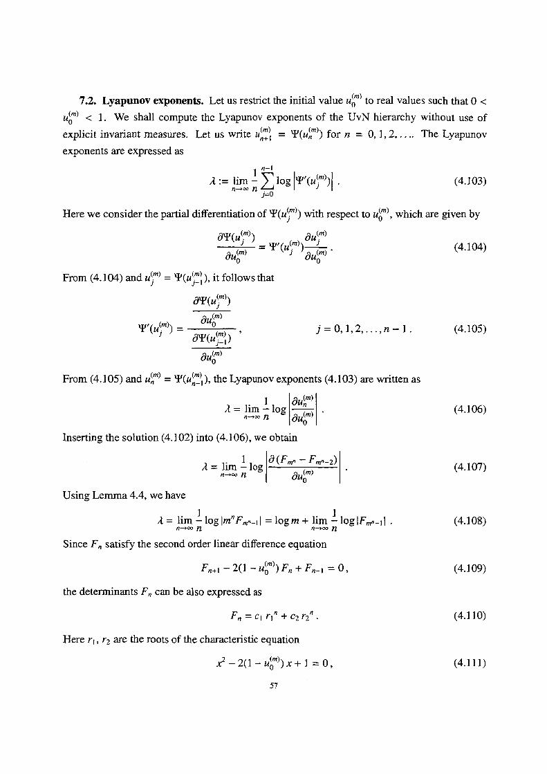
o.sSI) =91"("SM))o.',,m)'
From (4.104) and uS.M) = il'(uS.M-l), it follows that
oNl7(uSM')
Ou6m) "i"("S'M')= o,p(.s..-b , j=O•i•2,•••,n-i•
Ou8m)
From (4.I05) and uSM) = "P(uLM-),), the Lyapunov exponents (4.103) are written as
A. A-i.m. -i iog g:I:', •
Insening the solution (4.I02) into (4,l06), we obtain
0(Fmn -- Fnrn-2) 1 ,1 = .l-iM.. -. 10g o.8m) '
Using Lemma 4.4, we have
]1 1 = lim - log lm"F.n-il = Iogm+ lim - log IFmn-rl .
n-con n-conSince F. satisfy the second order linear difference equation
Fn+1 - 2(l - u8M)) Fn + Fn-1 = O,
the determinants F. can be also expressed as
Fn = ci rin + c2 r2n .
Here ri, r2 are the roots of the characteristic equation
x2 -2(1 -u8M))x+] = O,
57
7.2. Lyapunov exponents. Let us restrict the initial value u8M) to real values such that o <
u8M) < 1. We shall compute the Lyapunov exponents of the UvN hierarchy without use of
explicit invariant measures. Let us write uLM = NY(uÅíM)) for n = O, 1,2,.... The Lyapunov
exponents are expressed as
n-1 z:- Agm. -L2iog g"(uSm'). (4.io3)
j=oHere we consider the partial differentiation of NI'(uSpt>) with respect to u8M), which are given by
ONIf(u(.M)) Ou(.M)(4.104)
(4.105)
(4.106)
(4.107)
(4.108)
(4. 1 09)
(4.1lO)
(4.111)
and ci, c2 are determined by the initial condition. From the condition O < u8M) < 1, it follows
that lriI = lr21 = 1. Thus there exists a positive constant M such that O s IF.I < M. Moreover
we remove the zeros of F.n-i(u6M)) = O from the initial regi'on O < u8M) < 1, then we have
O < IF.l < M. Therefore we obtain Lo < logIF.n-il < Li, where Lo and Li are certain positive
constants. It is concluded that
lim llog lF.n-il =O. (4.l12) n-oo n
We can state:
THEoREM 4.3. Let us restrict the initial values u8M) to real values such that O < u8M) < l.
Then the Lyapunov exponents ofthe UvN hierarchy are log m.
8. Determinantal solutions for hierarchy of the Steffensen iteration
in this section, we give determinantal solutions for the discrete dynamical systems corre-
sponding to the eXtended Steffensen method which is proposed in Chapter 3.
Let us consider the quadratic equation
f(z) := z2+2bz+c=O, (4.113)
where z is a complex variable, and b, c are some complex constants. Rearranging Eq. (4.1 13),
we have the equation,
(a-b)z--c Z= z+(.+b) =: ip(Z)' (4•114)
where a is an auxiliary and arbitrary constant. We write the right hand side of Eq. (4.114)
as ip(z). We consider the extended Steffensen method (3.l8) for Eq. (4.1 13) with the simple
iteration function ip(z). The hierarchy of the Steffensen type iterations are gi'ven by
u:M.), = Åë.-i(uSM)), m= 2, 3, 4, ..., n:O, l, 2, ..., (4.ll5)
from (3.18). ln [6, 7], Arai, Okamoto, and Kametaka find a new addition formula for cot(x) in
terms of addition formulas for a three parameter family of functions. The aim of this section is
to obtain determinantal solutions for the hierarchy (4.I 15) by using a theorem in [6, 7].
To find solutions, we begi'n to consider the simple iteration
(a --' b) v. -' c , j= O, 1, 2,.... (4.116) Vn+1 = ip(Vn) = v. + (a + b)
We present addition formulas of v., which are resulted from the following theorem.
58
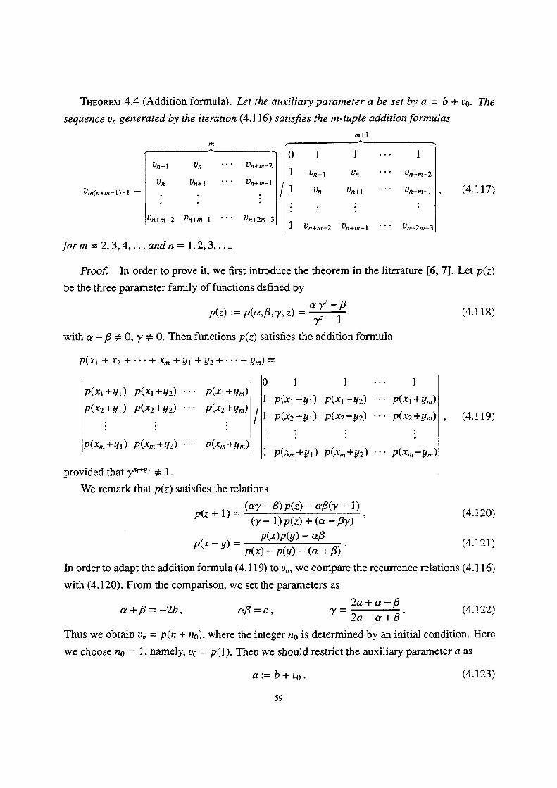
THEoREM 4.4 (Addition formula). Let the aLtxiliary parameter a be set by a = b + vo.
sequence v. generated by the iteration (4.1 l6) satisfies the m-tuple additionformulas
m+1 m-Vm(n+m-1)-1 =
Vn-1
Vn
.Vn+m-2
Vn Vn+1
'Vn+m-1
''' Vn+m-2
''' Vn+m-1
.''' Vn+2m-3
/
o
1
1
I
l
1
Vn-1
Vn
Vn+m-2
form = 2, 3, 4, ... and n= 1, 2, 3, ..-
Rroof.
be the three parameter fatnily of functions defined by
p(z) := p(a,5,xz) =
l
Vn Vn+1
l
Vn+m-1
1
Vn+m-2
Vn+m-l
Vn+2m-3
'
in order to prove it, we first introduce the theorem in the literature [6, 7].
a /4- -p 7Z -1with a -6 : O, 7 # O. Then functions p(z) satisfies the addition formula
P(Xl + X2 +'''+ Xm +Yl +Y2 +'''+ Ym) =
P(Xi +Yi)
P(X2+Yi)
P(Xm +Yl )
P(Xi +Y2)
P(X2 +Y2)
i
P(Xm+Y2)
P(JCi +Ym)
l7(X2+Ym)
i
••• p(xm+Ym)
/
o
1
1
E
1
1P(Xi +Yi)
P(X2+Yi)
P(.Xm+Yi)
lP(Xi + Y2)
P(X2+Y2) '''
I
P(Xm+Y2) '''
lP(.Xi +YM)
P(X2+Ym)
p(xm+Ym)
provided that •>tXi'Yj : 1 .
We remark that p(z) satisfies the re]ations
p(z + i) = (Eliillli{!ipPf,Z)) i iilll (..'>',ci;/ ;)i) ,
p(. . y) = p(.)p.(x:g)i(g6.s) .
In order to adapt the addition formula (4.119) to v.,
with (4.120). From the comparison, we set the parameters as
2a +a-6 a+6=-2b, a6=c, 7= 2a -a+6Thus we obtain v, = p(n + no), where the integer no
we choose no = l, namely, vo = p(]).
a := b+ vo .
S9
'
77ze
(4.1l7)
Let p(z)
(4.118)
(4.]19)
(4.I20)
(4.121)
we compare the recurrence relations (4.1 16)
. (4.122)
is determined by an initial condition. Here
Then we shou]d restrict the auxi]iary parameter a as
(4.123)
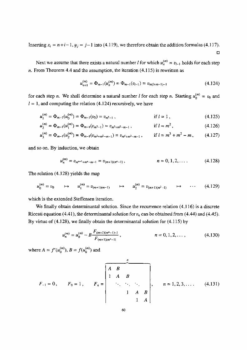
Inserting xi = n+i- 1, yj = j- 1 into (4.1 19), we therefore obtain the addition formulas (4.I 17).
m
Next we assume that there exists a natural number l for which uLM) = vi-i holds for each step
n. From Theorem 4.4 and the assumption, the iteration (4.1 15) is rewritten as
uSlllll •-- Åë.-1(uSM)) :Åë.-1(vl-1)= v.(l..-1)-1 (4.124)
for each step n. We shall determine a natural number l for each step n. Starting u8M) = vo and
l = 1 , and computing the relation (4. 1 24) recursively, we have
u:M)=O.-1(u8M))=O.-1(vo)=v.2-1, ift=l, (4.125) U(2M) = O.-l(UiM)) = O.-1(v.2-1) = v.3..2 -.-1 , ifl= m2, (4.1 26)
ugM) = Om-i(uSM)) = Åëm-i(vm3+m2-m-i) = v.4+.3-.-i , ifl= m3 +m2 -m, (4.l27)
and so on. By induction, we obtain
UÅíM) = Vmn"+mn -m.1 = V(m+1xmn-1), n= O, 1, 2, .... (4.128)
The relation (4.1 28) yields the map
u8M> =vo " uiM)= v(..1Å~.-1) H uSM) = v(..1Å~.2-1) H -•• (4.129)
which is the extended Steffensen iteration.
We finally obtain determinantal solution. Since the recurrence relation (4.1 16) is a discrete
Riccati equation (4.41), the determinantal solution for v. can be obtained from (4.44) and (4.45).
By virtue of (4.1 28), we finally obtain the determinantal solution for (4.1 15) by
uSm) = u8m) -- B FF/7ii llM(iil-: -' li', n= o, i, 2, ..., (4.i3o)
where A = f'(u6M)), B = f(u8M)) and
n - AB
IAB F-i=O, Fo=1, F,= '•. '•. '•. , n=1,2,3,.... (4.131) 1 AB IA
oo
It shou}d be noted that the determinantal solution (4.I30F(4.131) is also expressed as the
continued fraction
BB B uÅím)=u8M)----•••--. (4.i32) AA A . (m+1)(m't-1) We have constructed the deteminantal solution (4.l30)-(4.13l) by only using four arith-
metic operations. Here we ease this restriction. Let us allow to use the operation of square root.
Another type solution for (4.I15) is obtained by
uLm) =p(Ai, i2, :i/:lili; mn+i+mn-m) (4 i33)
from (4.1 1 8), (4.122), (4.128) and v. = p(n + l). Here ni and a2 denote the roots ofthe equation
f(z) = o.
9. Concluding remarks
ln this chapter, we have obtained the determinantal solutions for irreversib]e discrete equa-
tions. We have dealt with the hierarchy of the UvN system, and the hierarchies of discrete dy-
namical systems which are derived by applying the Newton type iterations and the Steffensen
type iterations to a quadratic equation. According to the setting of parameters and initial condi-
tions, these systems give rise to algorithms having higher order convergence rates, or solvable
chaotic systems. For alI cases, we have constructed the explicit solutions in a unified way.
Firstly, we have obtained the determinantal solutions v. for the second order Iinear differ-
ence equation and the discrete Riccati equation. We have derived the addition formulas for the
solutions v. (Theorems 4.I , 4.2, 4.4), At the next step, we have focused only on the values v.n
for integers m ) 2. Then we have introduced the new variab}es uiM) = v.n for each m. Finally,
we have showed that the addition formulas yield the irreversible dynamical systems of uLM). As
a result, we have derived the hierarchies of new solvable irreversible dynamical systems and
have obtained their determinantal solutions simultaneously.
From the determinantal solutions for the UvN hierarchy, we have obtained the Lyapunov
exponents of them without explicit use of invariant measures (Theorem 4.3).
61
CHAPTER 5
Concluding Remarks
ln this thesis, we have studied integrability of a continuous evolution equation and some
discrete equations. As an application of the soliton theory, we have proposed a numerical
algorithm based on the techniques in the nonlinear integrable systems.
In Chapter 2, we have considered the GDNLS equation. We first have constmcted the trav-
eling wave solution which is valid for any real values of parameters. We have applied the
Painleve test to the GDNLS equation for detecting integrability. We have shown that the equa-
tion possesses the Painleve property in a strict sense only for the known integrable cases of
parameters. Therefore we have shown that it possesses a conditional Painleve property for an
infinite number of cases of conditions for parameters, which is the same condition as that of
the single-valued property of the traveling wave solution. When the GDNLS equation has the
conditional Painleve property, it is necessary for the function ip(x, t) to satisfy an equation which
is transformed to the dispersionless KdV equation. We remark the interesting fact that the same
condition for ip(x, t) appeared at the Painleve analysis of the ]ong and short wave interaction
equation by Yoshinaga [87, 88]. Next we have examined stability of the solitary wave by the
numerical simulation. Remarkable difference between integrable case and non-integrable case
has not been observed, except for the quantities of ripples generated by interactions. The travel-
ing wave solution is stable in interactions and behaves like a soliton. In conclusion, the GDNLS
equation is a near-integrable system which has a conditional Painleve property and a stable
soliton-like traveling wave solution. Funher theoretical analysis on stability may be necessary.
ln Chapter 3, we have proposed an extension of the Steffensen iteration for finding a root a
of the nonlinear equation x = ip(x). We have developed the extended Steffensen method in terms
of the k-th Shanks transform which is a sequence convergence acceleration algorithm. The re-
suhing iteration method does not need any derivative. And it has a higher order convergence
rate, although the Shanks transform is originally a linearly convergent algorithm. If the equation
satisfies Åë'(a) : O, Å}1 , then the sequence generated by the extended Steffensen method has the
(k + 1)-th order convergence rate (Theorem 3.1). On the other hand, if the equation satisfies
ip'(a) = O, then the extended Steffensen iteration has remarkably the (k+2)2k-i-th order conver-
gence rate (Theorem 3.2). These theoretical convergence rates have been verified in numerical
62
examples (Examples 1, 2). For the implementation of the extended Steffensen iteration, the
s-algorithm is especially usefu1 to decrease the ainount of computations in the calculation of
Hankel determinants. This algorithm is stable for errors and equivalent to the discrete potential
KdV equation. Consequently, computation due to the numbers of mappings takes a major part
of the computational complexity. We have shown that the extended Steffensen iteration with
k = 2 has the minimal numbers of mappings in a special case of the Kepler equation (Example
3). Moreover, the extended Steffensen iteration converges for more cases ofparameters than the
Newton method.
in Chapter 4, we have obtained the determinantal solutions for irreversible discrete equa-
tions. We have dealt with the hierarchy of the UvN system, and the hierarchies of discrete
dynamical systems which are derived by applying the Newton type iterations and the Stef-
fensen type iterations to a quadratic equation. According to the setting of parameters and initial
conditions, these systems give rise to algorithms having higher order convergence rates, or solv-
able chaotic systems. For all cases, we have constructed the solutions in a unified way. Firstly,
we have obtained the determinantal solutions v. for some linear systems. We have derived the
addition formulas for the solutions v.. At the next step, we have focused only on the values v.n
for integers m ) 2. Then we have introduced the new variables uÅíM) = v.n for each m. Finally,
we have showed that the addition formu]as yield the irreversible dynamical systems of uiM). As
a result, we have obtained the hierarchies of new solvable irreversible dynamical systems and
their determinantal solutions simultaneously.
63
Acknowledgments
The author firstly wou]d like to thank al1 people who helped him with this thesis.
The author would like to express his deepest .qratitude to his supervisor, Professor Y. Naka-
mura, for continuous encouragements and many invaluable instructions. He also acknowledge
Professors M. Ohmiya, Y. Watanabe, and K. Kajiwara of Doshisha University for valuable ad-
vises and encouragements. He also thanks Dr. S. Tsujimoto and Dr. A. Nagai for many fruitful
discussions and helpfuI advises. The author is gratefu1 to whole members of Nakamura Labo-
ratory, Applied Mathematics Laboratory ofDoshisha University, and Suuri Kyoshitsu of Osaka
University for useful discussions and advises that enriched his study.
The author thanks Dr. T. Yoshinaga and Dr. H. Harada for useful comments and discussions
about the Painlev6 anaiysis. Thanks are also due to Mr. M. Deguchi and Mr. Y. Onoda for
assistance in numerical simulations of the GDNLS equation. He also thanks Dr. K. Umeno
for the fascinating lecture about solvable chaotic systems. The author would like to thank to
Professors T. Yamamoto, Y. Kametaka, H. Nagai, N. Osada, and H. Yoshida for giving him
helpful advises and suggestions.
The author finally would like to express his sincere gratitude to his parents.
M
[1]
[2]
[3]
[41
[5]
[6]
[7]
[8]
[9]
[1O]
[1 1]
[12]
[13]
[14]
[15]
[1 6]
[l7]
[1 8]
[19]
Bibliography
M. J. Ablowitz, A. Ramani, and H. Segur, Nonlinear evolution equations and ordinary differential equations
of Painleve type, Lett. Nuovo Cimento 23 (1978), 333-338.
M. J. Ablowitz, A. Ramani, and H. Segur, Aconnection between non}inear evolution and ordinary differential
equations of P-type I, J. Math. Phys. 21 (1980), 71 5-72l .
M. J. Ablowitz and H. Segur, Solitons and the Inverse Scattering Transform, SIAM, 1981 . `R. L. Adler and T. J. Riy]in, Ergodic and mixing properties of Chebyshev polynomials, Proc. Amer. Math.
Soc. 15 (1964), 794-796.
A. C. Aitken, On Bernoulli's numerical so]ution of algebraic equations, Proc. Roy. Soc. Edinburgh 46 (1926),
289-305.
M. Arai, K. Okarnoto, and Y. Kametaka, Aitken-Steffensen acceleration and a new additional formula for
Fibonacci numbers, Proc. Japan Acad. A 62 (1986), 5-7.
M. Arai, K. Okamoto, and Y. Kametaka, Aitken acceleration and Fibonacci numbers, Japan J. Appl. Math. 5
(1988), 145-152.
M. P. Bel]on, C.-M. Viallet, AIgebraic entropy, Commun. Math. Phys. 204 (1999), 425-437.
C. Brezinski, Acceleration de la conyergence en analyse numerique, Lecture Notes in Math. 584, Springer-
Verlag, Ber)in, 1977.
C. Brezinski, and R. Zagria, Extrapolation Methods: Theory and Practice, EIseyier, Amsterdam, 1991.
M. Bruschi, Determinanta1 solution of the ]ogistic map, J. Phys. A 31 (1 998), L153-L1 55.
F. L. Bauer, Nonlinear sequence transformations, Approximation of functions, Garbedian ed., Elseyier, New
York, 1965, 13zFl51.
F. Cajari, Historical note on the Newton-Raphson method of approxirnation, Amer. Math. Monthly 18 (191 l ),
F. Cariello and M. Tabor, Painleye expansions for nonintegrable evo]ution equations, Physica D 39 (1989),
77-94.
H. H. Chen, Y. C. Lee, and C. S. Liu, Integrability of nonlinear Hamilton systems by inverse scattering
method, Physica Scripta 20 (1979), 490-5oo.
G. Claessens, G. Loizou, and L. Wuytack, Comments on a root finding method using Pade approximation,
BIT 17 (1977), 360--361 .
P. A. Clarkson and C. M. Cosgroye, Painleye analysis of the non-]inear Schr6dinger family of equations, J.
Phys. A 20 (1987), 2003-2024.
D. A. Cox, The arithmetic-geomenic mean of Gauss, UEnseignement Mathematique 30 (1 984), 275-330.
A. Cuypt and L. Wuytack, Nonlinear Methodsin Numerical Analysis, North-Hol}and, 1987.
65
[20]
[21]
[22]
[23]
[24]
[25]
[26]
[27]
[28]
[29]
[30]
[31]
[32]
[33]
[34]
[35]
[36]
[37]
[38]
[39]
[40]
[41]
[42]
J. E. Dennis and R. B. Schnabel, Numerical Methods for Unconstrained Optimization and Nonlinear Equa-
tions, Prentice Hall, Englewood Cliffs, l983.
R. L. Devaney, An Introduction to Chaotic Systems, BenjaminlCummings, New York, 1986.
W. F. Ford andJ. A. Pennline, Acceleratedconyergence in Newton's method, SIAM Rev. 38 (I 996), 658-659.
C. S. Gardner, J. M. Greene, M D. Kruska}, and R. M. Miura, Method for solying the Korteweg-de Vries
equation, Phys. Rey. Lett 19 (1967), 1095-1097.
J. Gerlach, Acce}erated convergence in Newton's method, SIAM Rev. 36 (1 994), 272-276.
B. Grammaticos, A. Ramani, and V. Papageorgiou, Do integrable mappings have the Painleve property?,
Phys. Rey. Lett. 67 (1991), 1825-l 828.
A. Hasegawa and Y. Kodama, Solitons in Optical Communications, Clarendon Press, Oxford, l 995.
P. Henrici, Elements of Numerical Analysis, John Willey & Sons, New York, 1964.
J. Hietarinta and C. vaallet, Singularity confinement and chaos in discrete systems, Phys. Rey. Lett. 81 (1 998),
325-328.
R. Hirota and K. Suzuki, Studies on lattice solitons by using electrical networks, J. Phys. Soc. Japan 28
(1970), 1366-1367.
R. Hirota, Exact solution of the Korteweg-de Vries equation for multiple collisions of solitons, Phys. Rey.
Lett. 27 (l971), 1i92-1194.
R. Hirota, Exact three-soliton solution of the two-dimensional sine-Gordon equation, J. Phys. Soc. Japan 35
(1973), 1566.
R. Hirota, Exact envelope-soliton solution of a nonlinear wave equation, J. Math. Phys. 14 (1 973), 805-809.
R. Hirota, Exact N-soliton solutions of the waye equation of long waves in shallow-water and in nonlinear
lattices, J. Math. Phys. 14 (1 973), 81 O-814.
R. Hirota, Exact N-soliton solution of a nonlinear lumped network equation, J. Phys. Soc. Japan 35 (1973),
286-288.
R. Hirota, Exact N-soliton solution of nonlinear lumped self-dual network equations, J. Phys. Soc. Japan 35
( l 973), 289-294.
R. Hirota, A new form of Backlund transforrnations and its relation to the inverse scattering problem, Prog.
Theor. Phys. 52 (1974), 1498-l512.
R. Hirota and J. Satsuma, N-soliton solutions of nonlinear network equations describing a Vo]terra system, J.
Phys. Soc. Japan 40 (1976), 891-900.
R. Hirota and J. Satsuma, A variety of nonlinear network equations generated from the Backlund transforma-
tion for the Toda lattice, Supp. Prog. Theor. Phys. 59 (1 976), 64-1 OO.
R. Hirota, Non]inear partia] difference equations. I. A difference analogue of the Korteweg-de Vries equation,
J. Phys. Soc. Japan 43 (1977), 1424-I433.
R. Hirota, Nonlinear partial difference equations. II. Discrete-time Toda equation, J. Phys. Soc. Japan 43
(1977), 2074--2078.
R. Hirota, Nonlinear partial difference equations. III. Discrete sine-Gordon equation, J. Phys. Soc. Japan 43
(1977), 2079-2086.
R. Hirota Non]inear partial difference equations. IV. Backlund transformation for the discrete-time Toda
equation, J. Phys. Soc. Japan 45 (1978), 2079-2086.
66
[43]
[44]
[45]
[46]
[47]
[48]
[49]
[50]
[51]
[52]
[53]
[54]
[55]
[56]
[57]
[58]
[59]
[60]
[61]
[62]
[63]
R. Hirota and J. Satsuma, A simple structure of superposition formula of the Backlund transformation, J.
Phys. Soc. Japan 45 (1978), 1741-1750.
R. Hirota, Nonlinear partial difference equations. V. Nonlinear equations reducible to linear equations, J.
Phys. Soc. Japan 46 (1979), 312-319.
R. Hirota and M. Wadati, A functional integral representation of the soliton solution, J. Phys. Soc. Japan 47
(1979), 1385-l386.R. Hirota, S. Tsujimoto, and T. Imai, Difference scheme of soliton equations, Future Directions of Nonliriear
Dynamics in Physical andBiological Systems, P. L. Christiansen Ed., P}enum Press, 1993, 7-15.
R. Hirota, unpublished.
A. Iserles, Comp]ex dynamics and convergence acce}eration, IMA J. Numer. Anal. 11 (1 99l ), 205-240.
S. Kakei, N. Sasa, andJ. Satsuma, Bilinearization of a generalized deriyatiye nonlinear Schr6dinger equation,
J. Phys. Soc. Japan 64 (1995), 1519-1523.
D. J. Kaup and A. C. Newell, An exact solution for a derivative nonlinear Schr6dinger equation, J. Math.
Phys. 19 (1978) 798--801.
Y. Kodama and A. Hasegawa, Nonlinear pulse propagation in a monomode dielectric guide, IEEE J. QE-23
(1 987), 5 1 ()-524.
A. Kundu, Landou-Lifshitz and higher-odernonlinear systems gauge generated from nonlinear Schr6dinger
type equations, J. Math. Phys. 25 (l984) 3433-3438.
P. D. Lax, Integrals of nonlinear equations of evolution and solitary wayes, Comm. Pure App}. Math. 21
(1 968), 467-490.
M. Lyubich, The quadratic family as a qualitativeiy solvable model of chaos, Notices Arner. Math. Soc. 47
(2ooO),1042-1052.
A. Mukaihira and Y. Nakamura, Schur flow for orthogonal polynomials on the unit circle and its integrable
discretization, J. Comput. Appl. Math., to appear.
A. Nagai and J. Satsuma, Discrete soliton equations and convergence acceleration a)gorithms, Phys. Lett. A
209 (1995), 305-312.
A. Nagai, T. Tokihiro and J. Satsuma, The Toda mo]ecule equation and the s-algorithm, Math. Comput. 67
(1998), 1565-1575.
A. Nakamura and H. H. Chen, Multi-soliton of a deriyative Schrodinger equation, J. Phys. Soc. Japan 49
(1980), 8l3-816.
Y. Nakarnura, The BCH-Goppa decoding as a moment problem and a tau-function over finite fields, Phys.
Lett. A 223 (1 996), 75-81 .
Y. Nakamura, K. Kajiwara, and H. Shiotani, Ctri an integrable discretization of the Rayleigh quotient gradient
system and the power rnethod with a shift, J. Comput. Appl. Math. 96 (1 998), 77-90.
Y. Nakamura, Calculating Laplace transformations in terms of the Toda molecule, SIAM J. Sci. Comput. 20
(1998), 306-317.
Y. Nakamura, Algorithms associated with arithmetic, geometric and hamonic means and integrable systems,
J. Comput. Appl. Math., to appear.
T. Noda, The Aitken-Steffensen formula for systems ofnon]inear equations V, Proc. Japan Acad. A 68 (1 992),
37-40.
67
[64]
[65]
[66]
[67]
[68]
[69]
[70]
[71]
[72]
[73]
[74]
[75]
[76]
[77]
[78]
[79]
[80]
[8ll
[82]
[83]
[84]
[85]
[86]
[87]
A.-W. M. Nourein, Root deterrnination by use of Pade approximants, BIT 16 (1976), 291-297.
N. Osada, Extrapolation method for some singular fixed point sequences, Numer. Algorithms 3 (1992), 335-
344.
A. M. Ostrowski, So]ution of Equations and Systems of Equations, Second Edition, Academic Press, New
York, 1966.
H.-O. Peitgen and P R. Richter, The Beauty of Fractals, Springer-Verlag, 1986.
V. Papageorgiou, B. Grarnmaticos, and A. Ramani, Integrable lattices and conyergence acceleration algo-
rithms, Phys. Lett. A 179 (1993), 1 1 1-1 15.
S. Rabinovich, G. Berkolaiko, S. Buldyrev, A. Shehter and S. Havlin, "Logistic map": an analytical solution,
Physica A 218 (1995), 457460.
D. Shanks, Non-linear transformations of divergent and slow)y conyergent sequences, J. Math. and Phys. 34
(1955), 1-42.
G. E. Shilov, Linear Algebra, Dover, New York, 1977.
J. F. Steffensen, Remarks on iteration, Skand. Aktuar T:idskr. 16 (l933), 64-72.
W. W. Symes, The QR algorithm and scamering for the finite nonperiodic Toda lattice, Physica D 4 (1982),
275-280.
G. Szeg6, Onhogonal Polynomials, Colloquium Publications Vol. 23, Amer. Math. Soc., Proyidence, 1939.
M. Toda, Vibration ofa chain with nonlinear interaction, J. Phys. Soc. Japan 22 (1967), 431-436.
S. Tsujimoto, Studies on Discrete Nonlinear Integrable Systems, Doctor Thesis, Waseda Univ., 1 997.
S. M. Ularn and J. yon Neumann, On combination of stochastic and deterrninistic processes, the 53rd summer
meeting of AMS, Bul}. Amer. Math. Soc. 53 (1947), 1 l 20.
K. Umeno, Method of constructing exactly solvable chaos, Phys. Rev. E 55 (1997), 5280-5284.
K. Umeno, Superposition of chaotic processes with conyergence to Levy's stable ]aw, Phys. Rev. E 58 (1 998),
2644-2647.
K. Umeno, Exactly solyable chaos and addition theorems ofelliptic functions, RIMS Kokyuroku 1098 ( 1 999),
104-117.
R. Vein and P. Dale, Determinants and Their Applications in Mathematical Physics, Applied Mathematical
Sciences 134, Springer-Verlag, New York, 1999.
A. P. Veselov, wnat is an integrable mapping?, in: What Is Integrability`?, V. E. Zakharoy ed., Springer-Verlag,
Berlin, l991, 251-272.
M. Wadati, K. Konno, and Y. H. Ichikawa, A generalization of inverse scattering method, J. Phys. Soc. Japan
46 (1 979), 1965-1966.
J. Weiss, M. Tabor, and G. Carnevale, The Pain]eve property for partial differential equations, J. Math. Phys.
24 (1983), 522-526.
P. Wynn, On a device for computing the e.(S.) transformation, Math. Tables Aids Comput. 10 (l956), 9l-
96.
P. Wynn, On a procrustean technique for the numerical transformation of slowly convergent sequences and
series, Proc. Camb. Phi}. Soc. 52 (1956), 663-67 1 .
T. Yoshinagaand T. Kakutani, Solitary and e-shock wayes in a resonant system between long and short wayes,
J. Phys. Soc. Japan 63 (1994), 445-549.
68
[88]
[89]
T. Yoshinaga, Painleye analysis of the long and short wave interaction equation, J. Phys. Soc. Japan 64 (1995),
3193-3200.
N. J. Zabusky and M. D. Kruskal, Interaction of "solitons" in a co]lisionless plasma and the recurrence of
initial states, Phys. Rey. Lett. 15 (l965), 240-243.
69
List of Authors Papers Cited in the Thesis and Related Works
Original Papers
[1] Koichi Kondo, Kenji Kajiwara, and Kai Matsui, Solution and integrability of a gener-
alized derivative nonlinear Schr6dinger equation, J. Phy. Soc. Japan 66 (l 997), 60-66.
(Chapter 2)
[2] Koichi Kondo and Yoshimasa Nakamura, An extension of the Steffensen iteration and
its computational complexity, interdisciplinary information Sciences 4 (1998), 129-
l38. (Chapter 3)
[3] Koichi Kondo and Yoshimasa Nakarnura, Deterrninantal so]utions of solvable chaotic
systems, preprint. (Chapter 4)
Procee(lings Papers
[1 ] Koichi Kondo and Yoshimasa Nakamura, Newton-Steffensen-Shanks, RIMS Kokyuroku,
Kyoto Univ. iEteeEth-, rpNEEE, =a-' F > ' Xif77>t> ' 'S gr > ij X, J;r.asJlt"\`Xmpnc orI}IP)fitLE}f$P)tittst 1020 (1997), 28-38.
[2] Koichi Kondo and Yoshimasa Nakamura, A new iteration method of th'e Steffensen
type having higher order convergence rate, RIMS Kokyuroku, Kyoto Univ.
iiEteeElh-, rp*NtEEiE, fi' >kilS(JSI!'S-6 Steffensen #`Rffpt?ili, Sr.asJkc':'ip:i`XmpncorIillP.'i]tr
EE$P)f'i]=eq 1040 (1998), 228-236.
[3] Koichi Kondo and Yoshimasa Nakamura, Determinantal solutions for the Newton
method and so]vable chaotic systems, RIAM Kokyuroku, Kyushu Univ.
iEiasA-, P*NtEEjE,= L-b)iUia Erpt)ipJl-><(Dti5iiliEenc, fLblYJI<AL}'5LPESff]hNtF4I}f
t;7ti]tt EFflilFPytrtfiS?Willi 11ME-S4 (2ooO), 53-58.
[4] Satoshi Tsujimoto and Koichi Kondo, Molecule solutions of discrete soliton equations
and orthogonal po]ynomials, RIMS Kokyuroku, Kyoto Univ. i+L 7ls:fi, , i[i pt gA -, es lk JEf Pi ill O 5> ]:nc t SL s.2E !SEiift, F. as Jkc ALj)=4Xgptori}f :7,ti" fiE as
t:7tzitst 1170 (2000), 1-8.
70