IT 17 013

Examensarbete 30 hpFebruari 2017

System Dynamics Statistics (SDS)

A Statistical Tool for Stochastic System Dynamics Modeling and Simulation

Erik Gustafsson

Institutionen för informationsteknologiDepartment of Information Technology

2

Teknisk- naturvetenskaplig fakultet UTH-enheten Besöksadress: Ångströmlaboratoriet Lägerhyddsvägen 1 Hus 4, Plan 0 Postadress: Box 536 751 21 Uppsala Telefon: 018 – 471 30 03 Telefax: 018 – 471 30 00 Hemsida: http://www.teknat.uu.se/student

Abstract

System Dynamics Statistics (SDS)

Erik Gustafsson

This thesis is about the creation of a tool (SDS) for statistical analysis of stochasticSystem Dynamics models. System Dynamics is a specific field of simulation modelsbased on a system of ordinary differential equations and algebraic equations.

The tool is intended for analyzing stochastic System Dynamics models in various fieldsincluding biology, ecology, agriculture, economy, epidemiology, military strategy,physics, chemistry and many other fields. In particular, this project was initiated tofulfill the needs of a joint epidemiological project at Uppsala University (UU) andKarolinska Institute (KI). It is also intended to be used in basic courses in simulation atKI and the Swedish University of Agricultural Sciences (SLU).

A stochastic model has to be run a large number of times to reveal its behavior. TheSDS performs the analysis in the following way. First it connects to the SystemDynamics engine containing the model. Then a specified number of simulation runsare ordered. For each run the results of specified quantities are collected. From thecollected data, various statistical measures are calculated such as averages, standarddeviations and confidence intervals. The statistics can then be presented graphically inform of distributions, histograms, scatter plots, and box plots.

Finally, all features of SDS were thoroughly tested using manual testing. SDS wasthoroughly tested for statistical correctness, and then evaluated against somestochastic models.

Tryckt av: Reprocentralen ITCIT 17 013Examinator: Mats DanielsÄmnesgranskare: Bengt CarlssonHandledare: Mikael Sternad

4

Table of ContentsAbstract.................................................................................................................................31 Introduction.......................................................................................................................7

1.1 What is System Dynamics?........................................................................................71.2 Deterministic System Dynamics models...................................................................71.3 Stochastic System Dynamics Models........................................................................81.4 The history of System Dynamics.............................................................................101.5 Motivation for this project.......................................................................................10

2 Objectives........................................................................................................................113 Method.............................................................................................................................124 Evaluation of System Dynamics software and the choice of host simulation language. 13

4.1 Criteria for host simulation language.......................................................................131) Features.................................................................................................................132) Modifiability.........................................................................................................143) Compatibility........................................................................................................14

4.2 Candidate softwares.................................................................................................14 4.3 Conclusion..............................................................................................................164.4 Overview of chosen simulation language................................................................16

4.4.1 Insight Maker from the users point of view.....................................................164.4.2 Insight Maker from a technical point of view..................................................174.4.3 Principles behind Insight Maker's design.........................................................184.4.4 The structure of Insight Maker's code base......................................................19

5 The statistical tool............................................................................................................215.1 Design of the statistical tool.....................................................................................215.2 Technical specifications...........................................................................................215.3 Specification of the statistics and its presentations..................................................225.4 Implementation of the statistical tool.......................................................................235.5 Robustness tests of the tool......................................................................................23

6 The final product and its features....................................................................................246.1 The features of SDS.................................................................................................246.2 Additions made to Insight Maker.............................................................................26

6.2.1 Javascript engine for desktop application support...........................................276.2.2 Saving and loading local model files...............................................................27

7 Evaluation of SDS...........................................................................................................297.1 Evaluation of statistical correctness.........................................................................29

7.1.1 Evaluation Method...........................................................................................297.1.2 Evaluation of the results...................................................................................29

7.2 Evaluation with stochastic models...........................................................................337.2.2 A stochastic SIR model....................................................................................357.2.3 The deterministic Lanchester model................................................................377.2.4 The stochastic Lanchester model.....................................................................39

8 Discussion and conclusions.............................................................................................419 References........................................................................................................................43

5

6

1 IntroductionCompartment models are based on ordinary differential equations (ODEs). Such models have traditionally been deterministic, but during the last fifteen years, methods and technologies for introducing stochastics into the models have been developed. Four common types of stochastics (’transition stochasticity’, ’parameter stochasticity’, ’initial value stochasticity’ and’ signal stochasticity’) can be modeled with ordinary differential equations [1]. This knowledge makes System Dynamics models very powerful for a wide range of applications where stochasticity is important. However, the development of statistical tools in this field has not kept up with the development of the methodology.

1.1 What is System Dynamics?System Dynamics uses a graphical description to structure complex systems of differential equations and algebraic equations. This is an advantage at the structuring of the model, it facilities the programming, and it is of great pedagogic values when communicating with less mathematically experienced people [2], [3].

The most basic building blocks of System Dynamics are stocks and flows. Stocks represent a state, e.g. the level of water in a lake, or the number of inhabitants in a population. The flows represents the derivatives of the states, such as the rate of which water flows into the lake, or the rate of which inhabitants of the population are dying. For algebraic equations auxiliary symbols are used.

1.2 Deterministic System Dynamics modelsSystem Dynamics is a way to model a system of ordinary differential equations and algebraic equations. Differential equations are equations that relate the value of the function to its derivative. Most differential equations are not solvable with algebra, but solutions can be numerically approximated by algorithms to be evaluated in computer simulations.

Example 1: A deterministic model of radioactive decay

Assume that you want to model the decay process of X=20 radioactive atoms, where X(t) represents the number of (non-decayed) atoms at time t and the decay time constant T=10 time units.

This can be described by a difference equation (written in Euler’s form) initiated to 50

atoms and updated by an outflow for every small time-step Dt. Thus:

7

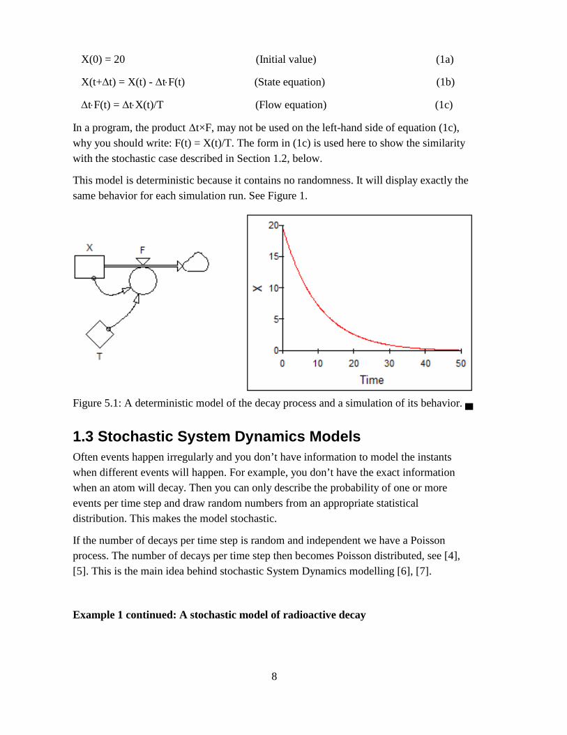
X(0) = 20 (Initial value) (1a)

X(t+Dt) = X(t) - Dt×F(t) (State equation) (1b)

Dt×F(t) = Dt×X(t)/T (Flow equation) (1c)

In a program, the product Dt×F, may not be used on the left-hand side of equation (1c), why you should write: F(t) = X(t)/T. The form in (1c) is used here to show the similarity with the stochastic case described in Section 1.2, below.

This model is deterministic because it contains no randomness. It will display exactly the same behavior for each simulation run. See Figure 1.

Figure 5.1: A deterministic model of the decay process and a simulation of its behavior. ▄

1.3 Stochastic System Dynamics ModelsOften events happen irregularly and you don’t have information to model the instants when different events will happen. For example, you don’t have the exact information when an atom will decay. Then you can only describe the probability of one or more events per time step and draw random numbers from an appropriate statistical distribution. This makes the model stochastic.

If the number of decays per time step is random and independent we have a Poisson process. The number of decays per time step then becomes Poisson distributed, see [4], [5]. This is the main idea behind stochastic System Dynamics modelling [6], [7].

Example 1 continued: A stochastic model of radioactive decay

8

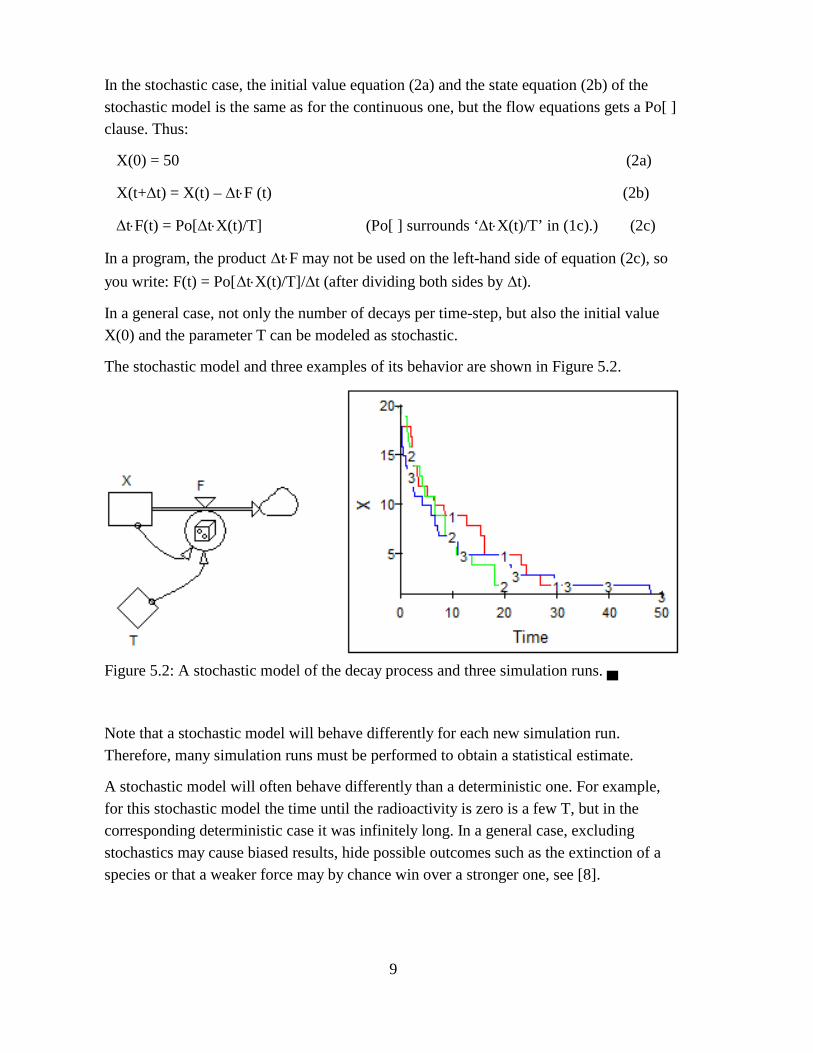
In the stochastic case, the initial value equation (2a) and the state equation (2b) of the stochastic model is the same as for the continuous one, but the flow equations gets a Po[ ] clause. Thus:

X(0) = 50 (2a)

X(t+Dt) = X(t) – Dt×F (t) (2b)

Dt×F(t) = Po[Dt×X(t)/T] (Po[ ] surrounds ‘Dt×X(t)/T’ in (1c).) (2c)

In a program, the product Dt×F may not be used on the left-hand side of equation (2c), so

you write: F(t) = Po[Dt×X(t)/T]/Dt (after dividing both sides by Dt).

In a general case, not only the number of decays per time-step, but also the initial value X(0) and the parameter T can be modeled as stochastic.

The stochastic model and three examples of its behavior are shown in Figure 5.2.

Figure 5.2: A stochastic model of the decay process and three simulation runs. ▄

Note that a stochastic model will behave differently for each new simulation run. Therefore, many simulation runs must be performed to obtain a statistical estimate.

A stochastic model will often behave differently than a deterministic one. For example, for this stochastic model the time until the radioactivity is zero is a few T, but in the corresponding deterministic case it was infinitely long. In a general case, excluding stochastics may cause biased results, hide possible outcomes such as the extinction of a species or that a weaker force may by chance win over a stronger one, see [8].

9

For this project, the essential insight is that a stochastic model requires a large number of simulations to generate probability functions of results from which statistical estimates can be derived.

1.4 The history of System DynamicsSystem Dynamics is a way to construct a complex mathematical model of differential equations in a graphical way that can be easily be understood. This approach was inventedat MIT by Jay W. Forrester. The first applications for System Dynamics was developed for General Electric and simulated management and economical systems. Later System Dynamics was adopted by many other fields such as biology, ecology, agriculture, economy, epidemiology, military strategy, physics, chemistry and many other fields. The first System Dynamics software was SIMPLE (1958) [9] and soon after that DYNAMO (1959) [10], [11]. However, these softwares did not have a graphical interface to construct the models. With Stella [12] and Powersim [13] you could graphically construct the model in a drag-and-drop manner using a small number of symbols such as stock, Flow, Auxiliary and constant. Then, by clicking in such a symbol, a dialog appeared where the user could insert equations and numbers. Today there exist a variety of System Dynamics software packages of which most have a graphical user interface for System Dynamics modeling.

1.5 Motivation for this projectDeterministic System Dynamics models always generate exactly the same result, which hides a lot of the information of e.g. variations and even may distort the results. The difference can be compared to an average value versus a distribution. The distribution gives a lot more information than just the average, such as the variance, but also the shapeof the distribution which tells if all the outcomes are equally likely or there might be several different peaks where the outcome is likely to be.

The purpose of this project was to construct a tool for stochastic and dynamic modeling for simulation of compartment models at Uppsala University, the Swedish University of Agricultural Sciences and Karolinska Institute (with which the department of Signals and Systems cooperates both in research and teaching). “Development of such a tool will dramatically improve the possibility to work with realistic compartment models within a large number of fields such as biology, ecology, medicine, epidemiology, economy, etc.” [14].

10

2 ObjectivesThe goals of this project are:

To construct a tool for analyzing statistics in stochastic System Dynamics models.

The tool should be able to visualize statistical distributions of results from the simulation of System Dynamics models. The tool should also be able to find correlations between results, such as how an increase in X is related to the value of Y.

To evaluate this tool against a set of System Dynamics standard models.

The tool should be evaluated against a set of standard models to see how useful the tool isfor its intended application.

It is important that the statistical tool can be publicly available, which makes open source preferable if possible. It is also preferable have a graphical user interface which most modern tools have, it should also have support for the discrete distribution used in transition stochastic simulations namely Poisson.

11

3 MethodTo create a statistical tool for System Dynamics, it is necessary to have an engine for running System Dynamics models. We could create one from scratch, but that would be very time consuming and also a bad idea since there are many System Dynamics environments available that can be used, and they already have many users.

Instead we choose to evaluate some of the most common System Dynamics languages and evaluate them to the requirements of this project. From these evaluation one host languages is selected. This is described in section 4.

One important aspect is the method for communication between the tool and the host language. The tool can either be integrated with the host language, or it can connect to thehost language with an API.

Thereafter the tool for calculating statistical measures and visualizing the data are developed. This is described in section 5.

Finally, the tool is evaluated against stochastic versions of two standard System Dynamic models, namely the SIR model modeling the spread of a diseases and Lanchester’s model describing two forces trying to take out each other. This is done in section 6.

12

4 Evaluation of System Dynamics software and the choice of host simulation language

4.1 Criteria for host simulation languageIn order to create a statistical tool for System Dynamics we need a host environment in form of a simulation language to which we can implement our tool. To find a suitable candidate we have three criteria given by the project: 1) It should have features related to this project, in particular random number generators for various statistical distributions is necessary. 2) It should be able to modify. Preferably, it should be open source so that the source code could be modified. A second option would be to connect to the host software with an external API. 3) It should preferably be platform independent so it could be used in various computer environments with different hardware and operative systems.

We denote the three criteria: 1) Features, 2) Modifiability and 3) Compatibility.

1) FeaturesSince this work is focused on stochastic model studies, we need random number generators for the most common distributions. In particular, RNGs for uniform, Poisson, exponential, and normal distributions are necessary.

We also need support for a System Dynamics User Interface (UI).

Random number generators (RNG)

Many models are based on discrete entities such as humans, rabbits, cars, atoms, etc. The number of transitions between compartments then has to be integer. Then the number of transitions during a time step becomes Poisson distributed. To model this, a random number generator for the Poisson distribution is necessary [6], [7]. For Stochastic parameters and initial values various types of random number generators are necessary.

System Dynamics UI

There are many ways of modeling differential equation systems. It can be done by directlycoding the equations in a general purpose programming language. However, the System Dynamics approach to build the model with stocks, flows etc., using a drag-and-drop manner has a number of advantages of pedagogic art, possibility to communicate and visual overview.

13

2) ModifiabilityModifiability can be achieved in two ways, either by directly editing the source code of the host program or by using an external API.

Modification of the open source code

If the source code is open and available we can go into the System Dynamics software and add our code directly, and make changes to the software that would be useful to us.

Open source not only has the advantage that the software can be modified, it also enables legal redistribution of our software package with the host environment included.

Controlled from external API

A second option is to control the software from an external API. If we cannot modify the software itself we can at least control it from the outside.

3) Compatibility

Platform independence

It is preferable that the software will work on different platforms. If the software runs on avirtual machine like Java, or interpreter such as Javascript or Python, they will be able to run on any platform that has this virtual machine or interpreter. If the software is specifically written and works for one operative system it might not sustain for the future if hardware and operative systems changes over time.

4.2 Candidate softwaresTo find a suitable candidate for this project we first selected seven of the most interesting candidates, here presented in alphabetic order: DYNAMO Professional Plus v. 3.1 [11], Insight Maker v. 5 [15], Matlab-Simulink 8.6 [16], [17], Powersim Studio 10 [18], Pyndynamics 29-06-2016 [19], Simantics v 1.9.0 [20] and Stella v10.1.2 [21].

14

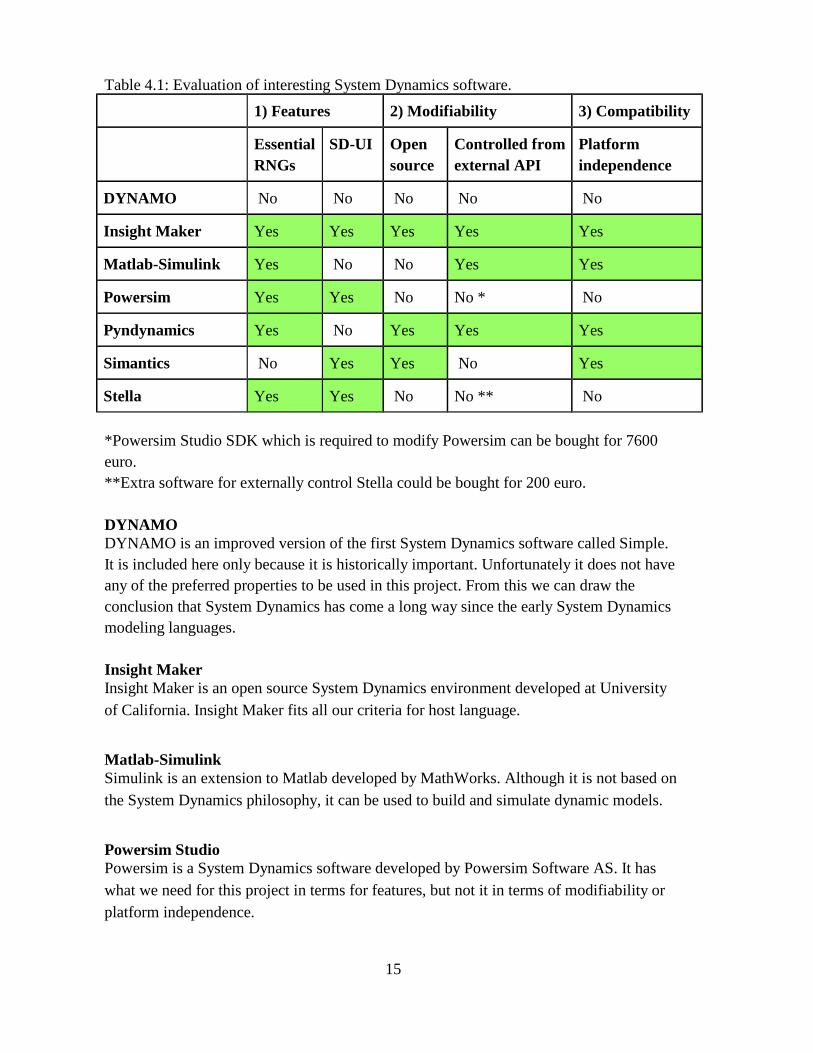
Table 4.1: Evaluation of interesting System Dynamics software.

1) Features 2) Modifiability 3) Compatibility

EssentialRNGs

SD-UI Open source

Controlled fromexternal API

Platform independence

DYNAMO No No No No No

Insight Maker Yes Yes Yes Yes Yes

Matlab-Simulink Yes No No Yes Yes

Powersim Yes Yes No No * No

Pyndynamics Yes No Yes Yes Yes

Simantics No Yes Yes No Yes

Stella Yes Yes No No ** No

*Powersim Studio SDK which is required to modify Powersim can be bought for 7600 euro.**Extra software for externally control Stella could be bought for 200 euro.

DYNAMODYNAMO is an improved version of the first System Dynamics software called Simple. It is included here only because it is historically important. Unfortunately it does not have any of the preferred properties to be used in this project. From this we can draw the conclusion that System Dynamics has come a long way since the early System Dynamics modeling languages.

Insight MakerInsight Maker is an open source System Dynamics environment developed at University of California. Insight Maker fits all our criteria for host language.

Matlab-SimulinkSimulink is an extension to Matlab developed by MathWorks. Although it is not based on the System Dynamics philosophy, it can be used to build and simulate dynamic models.

Powersim StudioPowersim is a System Dynamics software developed by Powersim Software AS. It has what we need for this project in terms for features, but not it in terms of modifiability or platform independence.

15

PyndynamicsPyndynamics is an open source System Dynamics software developed at Bryant University. It does not have a System Dynamics UI, but it has all needed RNGs. It can also be controlled from an external API.

SimnaticsSimnatics is an open source System Dynamics environment developed by VTT Technical Research Centre of Finland. It does not have an external API or support for different statistical distributions that we require.

StellaStella is a System Dynamics software developed by ISEE systems. As with Powersim, Stella also has what this project needs in terms of features but not in terms of modifiability or platform independence.

4.3 ConclusionThe only evaluated software that fits all of our requirements is Insight Maker. It is modifiable, platform independent and has all the features we need. It is also open source which was a desired property in the specification of this project. The big commercial alternatives Powersim and Stella also have all the features that we were looking for, but they don’t have the possibility for modifications or the cross platform compatibility. Otheropen source alternatives such as Simnatics don’t have the features we need in terms of statistical distributions.

4.4 Overview of chosen simulation languageThe chosen tool decided in section 4.1 is Insight Maker. Insight Maker is developed by Scott Fortmann-Roe at University of California, Berkeley. It is a simulation language usedfor both System Dynamics and agent based modeling, of which we only look at the System Dynamics part in this paper. Fortmann-Roe describes his work in the paper “A general-purpose tool for web-based modeling & simulation” [22]. The original version of Insight Maker is developed primarily for running on the web, but since it is written in Javascript it can also be executed as a desktop application in a Javascript engine such as NodeWebkit.

4.4.1 Insight Maker from the users point of viewThe user interface consists of three main components: toolbar, model diagram and configuration panel. The toolbar is where tools are selected by the user. A tool can be a

16

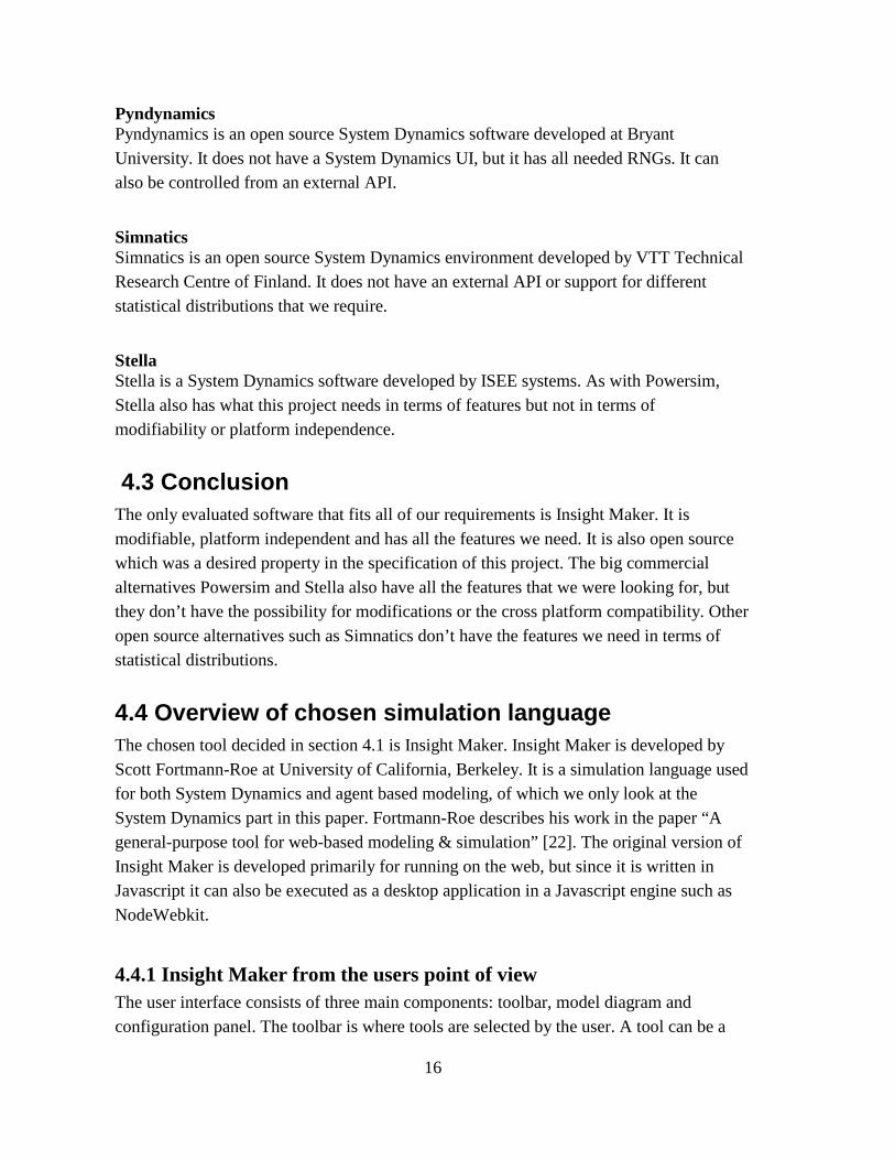
System Dynamics component such as a Stock or a Flow. It can also be a pedagogic component such as a text or an image for explaining the model. When a tool is selected the components are placed on the model diagram which visualizes and keeps the models together. After the components have been created they can be specified with configuration panel to set properties such as name and initial value or equation.

Figure 4.1: Insight Maker's user interface has three main components: 1. Toolbar, 2. Model Diagram and 3. Configuration Panel.

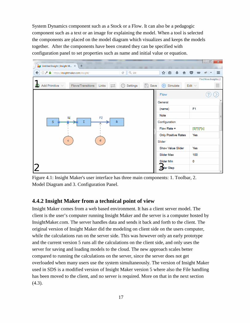
4.4.2 Insight Maker from a technical point of viewInsight Maker comes from a web based environment. It has a client server model. The client is the user’s computer running Insight Maker and the server is a computer hosted byInsightMaker.com. The server handles data and sends it back and forth to the client. The original version of Insight Maker did the modeling on client side on the users computer, while the calculations run on the server side. This was however only an early prototype and the current version 5 runs all the calculations on the client side, and only uses the server for saving and loading models to the cloud. The new approach scales better compared to running the calculations on the server, since the server does not get overloaded when many users use the system simultaneously. The version of Insight Makerused in SDS is a modified version of Insight Maker version 5 where also the File handlinghas been moved to the client, and no server is required. More on that in the next section (4.3).

17

Figure 4.2: Client Server model used in original Insight Maker. Image from Wikipedia.

4.4.3 Principles behind Insight Maker's designWhen developing software one has to make prioritization between features, accessibility and performance [22].

Features vs. accessibility: A software with a lot of features might get non-transparent andoverwhelm the user with all of its features. It is much harder for a user to navigate in a user interface crowded with a lot of visible features compared to one with only a few.

Accessibility vs. performance: A software that have very huge overhead in terms of visualization utilizes system resources to help the user, which might lead to lower performance. If the system did not have a user interface but only command line it could most likely go faster because it does not have to take accessibility into account.

Performance vs. features: Having a lot of features might slow the software as the software grows and becomes bloated with long loading times and huge memory management overhead.

In the case of Insight Maker Fortmann-Roe has decided to make the prioritization in this order: Accessibility first, Features second and performance last. This does not mean that the performance of Insight Maker is bad. It only means it is the last priority after accessibility and feature when the software was designed.

18

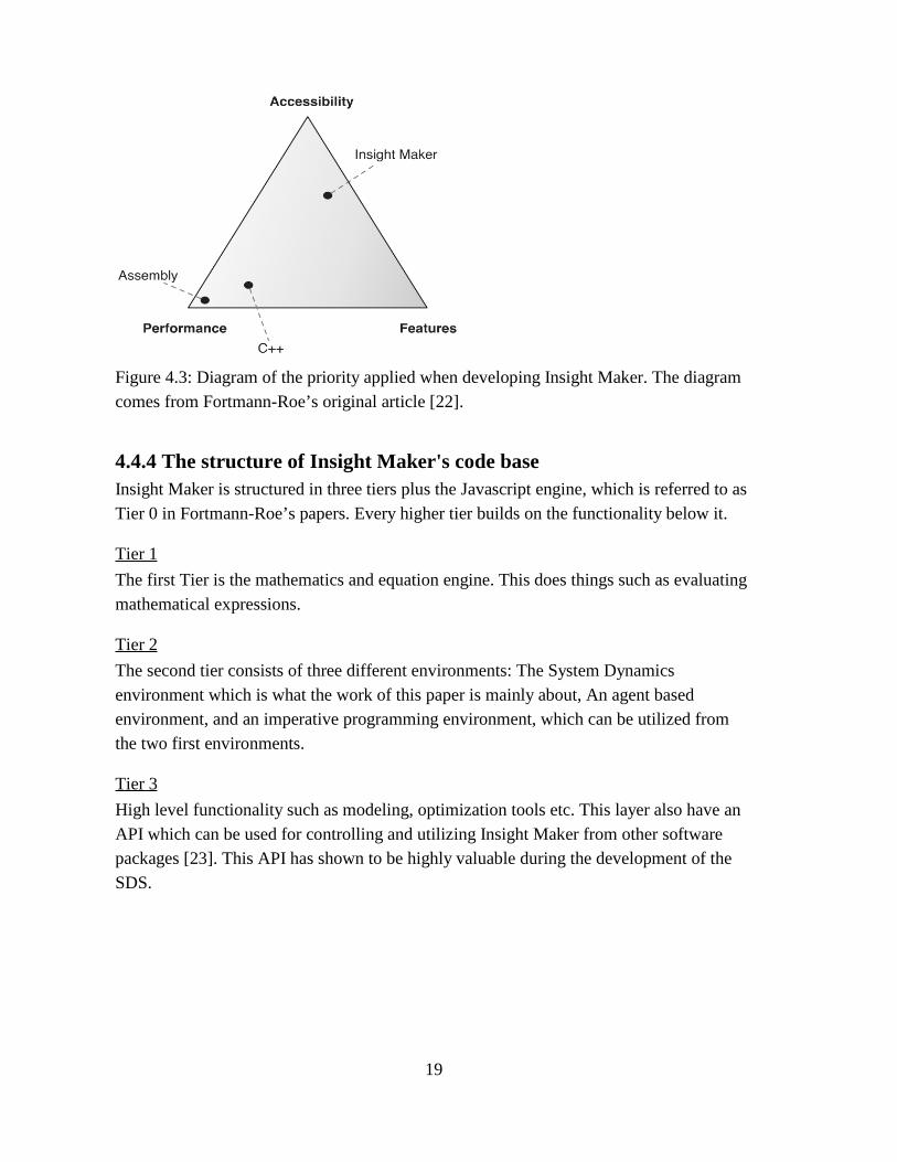
Figure 4.3: Diagram of the priority applied when developing Insight Maker. The diagram comes from Fortmann-Roe’s original article [22].

4.4.4 The structure of Insight Maker's code baseInsight Maker is structured in three tiers plus the Javascript engine, which is referred to asTier 0 in Fortmann-Roe’s papers. Every higher tier builds on the functionality below it.

Tier 1

The first Tier is the mathematics and equation engine. This does things such as evaluating mathematical expressions.

Tier 2

The second tier consists of three different environments: The System Dynamics environment which is what the work of this paper is mainly about, An agent based environment, and an imperative programming environment, which can be utilized from the two first environments.

Tier 3

High level functionality such as modeling, optimization tools etc. This layer also have an API which can be used for controlling and utilizing Insight Maker from other software packages [23]. This API has shown to be highly valuable during the development of the SDS.

19

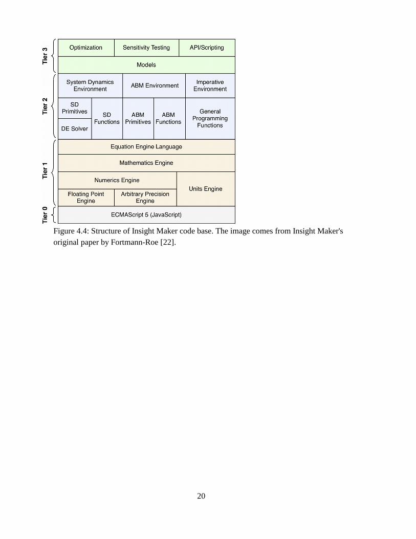
Figure 4.4: Structure of Insight Maker code base. The image comes from Insight Maker's original paper by Fortmann-Roe [22].

20

5 The statistical tool

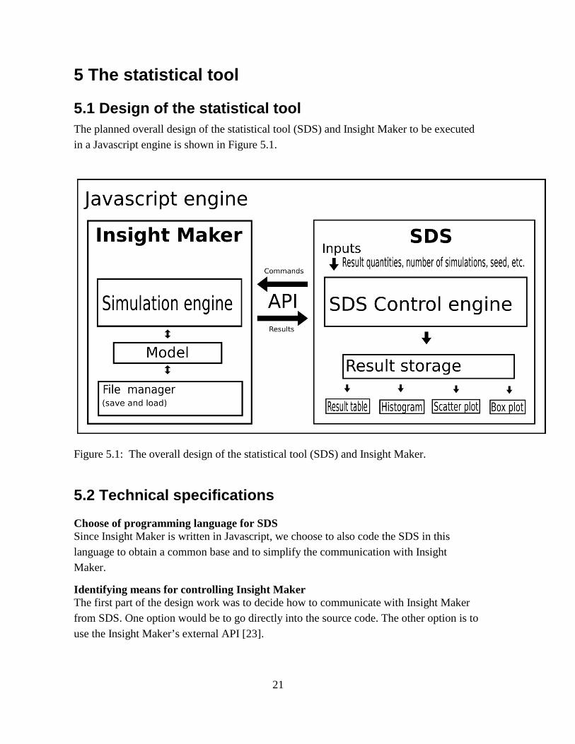
5.1 Design of the statistical toolThe planned overall design of the statistical tool (SDS) and Insight Maker to be executed in a Javascript engine is shown in Figure 5.1.

Figure 5.1: The overall design of the statistical tool (SDS) and Insight Maker.

5.2 Technical specifications

Choose of programming language for SDSSince Insight Maker is written in Javascript, we choose to also code the SDS in this language to obtain a common base and to simplify the communication with Insight Maker.

Identifying means for controlling Insight MakerThe first part of the design work was to decide how to communicate with Insight Maker from SDS. One option would be to go directly into the source code. The other option is to use the Insight Maker’s external API [23].

21

It was concluded that using the API is the best choice, because it makes it easy to maintain the tool for use with future versions of Insight maker. However, some code was added directly to Insight Maker's source code for adding an offline file handler, and for adding communication features to the API to make it easier to integrate with. This also has the benefit that the SDS can be turned on and off from Insight Maker.

User inputsThe user must be able to specify what model quantities to analyze and present. It should also be possible to specify the number of simulation runs. Further, there should be a number of options. For example, the possibility to provide a seed to the model enables thestudy to be reproducible, and a ‘Skip-on-condition’ option can save execution time when only some of the simulation runs will produce interesting results to be analyzed.

The SDS control engineSDS uses Insight Makers API to send requests for running the simulation of the loaded model. Insight Maker then sends the result of the simulation run back. This process is repeated until the specified number of runs is executed. The collected data are put into a result storage. These data are then used for analysis and presentation in different subprograms as shown in Figure 5.1.

5.3 Specification of the statistics and its presentationsThe collected and stored data from multiple simulation runs should now be analyzed and presented in different ways. The full information of the data are a joint distribution function. This cannot be visualized for many result quantities.

Therefore, we have chosen to present fundamental statistics for each specified result, suchas average, standard deviation, confidence interval, mean, max, percentile quantity in the Result Table.

Further, it should be possible to display the results in form of:

• Histogram, which can visualize the statistical distribution of a result quantity.

• Scatter Plot, which visualize one quantity versus another. Also the correlation coefficient between the quantities is here calculated.

• Box Plot, where comparisons of quartiles and extreme values can be compared between different quantities.

To make the results available for further analysis, export of the data in unsorted or sorted form should be possible.

22

5.4 Implementation of the statistical tool

The work to implement SDS included various types of work such as:

• Exploring and understanding Insight Maker’s capability for stochastic models.

• Studying structure and the code of Insight Maker.

• Studying the properties and functions of Insight Maker’s external API.

• Implementing a connection between SDS and Insight Makers using the API.

• Evaluating alternative Javascript engines.

• Survey of the statistical literature for formulas and descriptive statistics.

• Implementing programming modules for statistic analysis.

• Designing and implementing a graphical user interface for SDS.

• Implemented modules for visualization of the statistical data.

We will not go into details of this work, which together with the testings consumed the major part of this thesis project. In short, all specifications were successfully implemented. The final SDS is presented in the next section.

5.5 Robustness tests of the toolA large number of tests have been performed to make the statistical tool robust with respect to invalid inputs, and incomplete specifications. Especially this prevents the system to crash during a session. For example it is important that the specified result quantities exist in the model. Further we put a big amount of work into making reset, halt and continue to work as intended. All detected errors were corrected.

23

6 The final product and its featuresThe final product contains both the SDS and a slightly modified version of Insight Maker version 5.

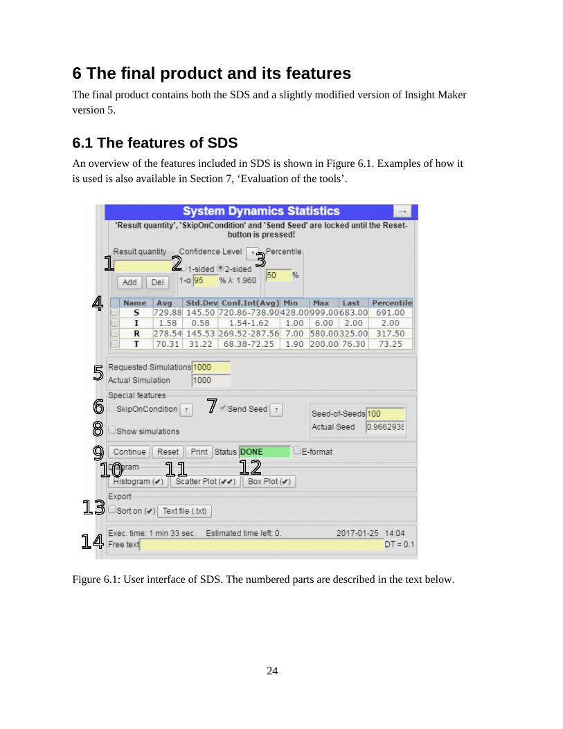
6.1 The features of SDSAn overview of the features included in SDS is shown in Figure 6.1. Examples of how it is used is also available in Section 7, ‘Evaluation of the tools’.

Figure 6.1: User interface of SDS. The numbered parts are described in the text below.

24

Features shown in Figure 6.1:

1. Specification of result quantities to be studied

2, 3. Specification of confidence level and percentiles

4. Result Table presenting Average, Standard deviation, Confidence interval, Min, Max, Value from last simulation, and percentile for each specified quantity.

5. Specification of requested number of simulations.

6. SkipOnConditionIn some stochastic models not all simulation runs may be of interest. For example, you might be interested only in simulation runs where an epidemic outbreak happens. In this case the user can create a condition to skip simulation runs where, say, less than 50 persons get the disease.

7. Send SeedWhen reproducibility is important, the initial seed of the simulations can be set from SDS.Then the series of simulation runs can later be reproduced. This feature is also useful for variance reduction.

8. Show simulationsSDS has the ability to show a diagram over every simulation while it runs. This is good for understanding the model and debugging it, but it slows down the execution why the default is to have this feature disabled.

9. Command buttons, current status and presentation in e-format

10. Histogram of produced dataThe histogram can be used to visualize the statistical distributions of the studied quantities.

11. Scatter Plot and correlationA scatter plot (also called XY-plot) displays the results of two quantities as a point in an XY diagram for each simulation run. Also the correlation coefficient between the quantities is here calculated and presented.

12. Box Plot for comparing distributionsA box plot gives a quick overview of selected quantities in terms of quartiles and extreme values.

13. Exporting of dataIf you want to analyze or present the results in ways not supported by SDS, you can export the results to a text file for further analysis or presentation. Here you can also have the result quantities sorted after the size of a specified quantity. The exported file has the

25

TSV format (Tab Separated Values) [24], which can be imported into excel or other spreadsheets for further calculations or visualizations.

14. Technical information and free text.The execution time, date and time for the study, time step used in the model is here recorded. You also have the possibility to write a short comment about the model or session here.

Integrated help systemSDS has an integrated help system containing texts and illustrations about some of the features. This help can be accessed through the question mark button [?]. ‘Confidence level’, ‘SkipOnCondition’ and ‘Send Seed’ have help buttons for displaying more information.

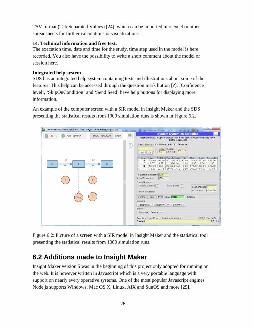
An example of the computer screen with a SIR model in Insight Maker and the SDS presenting the statistical results from 1000 simulation runs is shown in Figure 6.2.

Figure 6.2: Picture of a screen with a SIR model in Insight Maker and the statistical tool presenting the statistical results from 1000 simulation runs.

6.2 Additions made to Insight MakerInsight Maker version 5 was in the beginning of this project only adopted for running on the web. It is however written in Javascript which is a very portable language with support on nearly every operative systems. One of the most popular Javascript engines Node.js supports Windows, Mac OS X, Linux, AIX and SunOS and more [25].

26

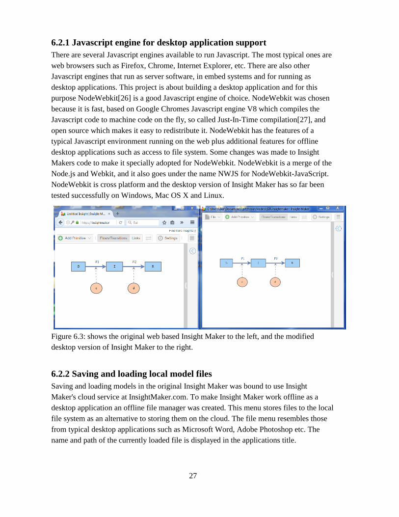
6.2.1 Javascript engine for desktop application supportThere are several Javascript engines available to run Javascript. The most typical ones are web browsers such as Firefox, Chrome, Internet Explorer, etc. There are also other Javascript engines that run as server software, in embed systems and for running as desktop applications. This project is about building a desktop application and for this purpose NodeWebkit[26] is a good Javascript engine of choice. NodeWebkit was chosen because it is fast, based on Google Chromes Javascript engine V8 which compiles the Javascript code to machine code on the fly, so called Just-In-Time compilation[27], and open source which makes it easy to redistribute it. NodeWebkit has the features of a typical Javascript environment running on the web plus additional features for offline desktop applications such as access to file system. Some changes was made to Insight Makers code to make it specially adopted for NodeWebkit. NodeWebkit is a merge of the Node.js and Webkit, and it also goes under the name NWJS for NodeWebkit-JavaScript. NodeWebkit is cross platform and the desktop version of Insight Maker has so far been tested successfully on Windows, Mac OS X and Linux.

Figure 6.3: shows the original web based Insight Maker to the left, and the modified desktop version of Insight Maker to the right.

6.2.2 Saving and loading local model filesSaving and loading models in the original Insight Maker was bound to use Insight Maker's cloud service at InsightMaker.com. To make Insight Maker work offline as a desktop application an offline file manager was created. This menu stores files to the localfile system as an alternative to storing them on the cloud. The file menu resembles those from typical desktop applications such as Microsoft Word, Adobe Photoshop etc. The name and path of the currently loaded file is displayed in the applications title.

27

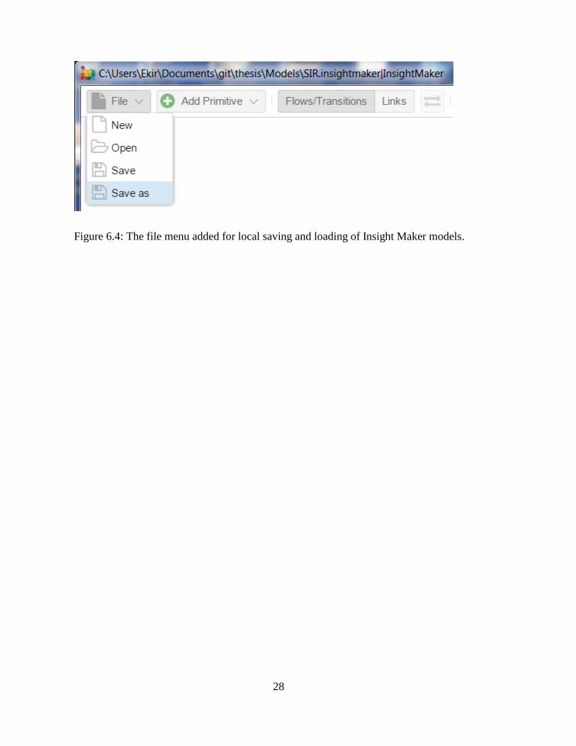
Figure 6.4: The file menu added for local saving and loading of Insight Maker models.

28

7 Evaluation of SDSAll features of SDS were thoroughly tested using manual testing. SDS was thoroughly tested for statistical correctness, and then evaluated against some stochastic models as described below.

7.1 Evaluation of statistical correctnessWe wanted to evaluate the statistical correctness both for Insight Maker and SDS. The statistical correctness of Insight Maker means that the random numbers from the statistical distributions should be correct. SDS can estimate the distributions from Insight Maker by repeated runs. Then we can compare the estimated values with the theoretical ones.

7.1.1 Evaluation MethodThe primary estimates to be evaluated are the average and the standard deviation of the distributions to see if they are consistent with those of the theoretical distributions.

To do this, a small Insight Maker model was built that generates rectangular, Poisson, binomial, normal, and exponential distributed random numbers.

The model was then executed 100,000 times, from which SDS calculated the averages and standard deviations. The results from the simulations was then compared with the theoretical averages and standard deviations of these distributions. The distributions of thecollected data was also studied using the histogram facility.

7.1.2 Evaluation of the resultsWe here used the ‘Seed of seeds’ set to 1, so that this study can be reproduced. We now proceed by calculating the theoretical averages and standard deviations for these distributions [4], [5] to see if they agree with estimates from SDS. The SDS results from the 100,000 simulation runs are shown in Figure 7.1.

29

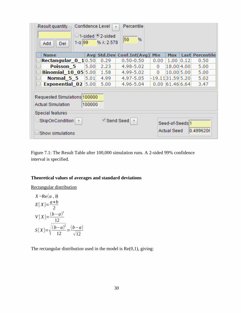
Figure 7.1: The Result Table after 100,000 simulation runs. A 2-sided 99% confidence interval is specified.

Theoretical values of averages and standard deviations

Rectangular distribution

X ~Re(a , b)

E [X ]=a+b

2

V [X ]=(b−a)2

12

S [X ]=√ (b−a)2

12=(b−a)

√12

The rectangular distribution used in the model is Re(0,1), giving:

30

X ~Re(0,1)

E [X ]=0+1

2=0.50

S [X ]=(1−0)

√12=1/√12≈0.29

The estimated values for the rectangular distribution were E[X] ≈ 0.50 and S[X] ≈ 0.29. The theoretical average 0.50 is within the 99% level confidence interval of the measured average.

Poisson distribution

X ~Po( λ)E [X ]=λV [X ]=λS [X ]=√λ

The Poisson distribution used in the model is Po(5), giving:

X ~Po(5)E [X ]=5.00V [X ]=5.00S [X ]=√5.00≈2.24

The estimated values for the Poisson distribution were E[X] ≈ 5.00 and S[X] ≈ 2.23. The theoretical average 5.0 is within the 99% level confidence interval of the measured average.

Binomial distribution

X ~Bin (n , p)E [X ]=n∗pV [X ]=n∗p∗qS [X ]=√n∗p∗q

The Binomial distribution used in the model is Bin(10, 0.5), giving:

31

X ~Bin(10, 0.5)E [X ]=10∗0.5=5.00V [X ]=10∗0.5∗0.5=2.50S [X ]=√2.50≈1.58

The estimated values for the binomial distribution were E[X] ≈ 5.00 and S[X] ≈ 1.58. Thetheoretical average 5.0 is within the 99% level confidence interval of the measured average.

Normal distribution

X ~N(μ ,σ)E [X ]=μ

V [X ]=σ2

S [X ]=σ

The Normal distribution used in the model is N(5, 5), giving:

X ~N(5,5)E [X ]=5.00V [X ]=5.002

=25.00S [X ]=5.00

The estimated values for the normal distribution were E[X] ≈ 5.01 and S[X] ≈ 4.99. The theoretical average 5.0 is within the 99% level confidence interval of the measured average.

Exponential distribution

X ~Exp(λ )

E [X ]=1λ

V [X ]=1

λ2

S [X ]=1λ

The Exponential distribution used in the model is Exp(0.2), giving:

32

X ~Exp(0.2)

E [X ]=1

0.2=5

V [X ]=1

0.22=25

S [X ]=5

The estimated values for the exponential distribution were E[X] ≈ 5.00 and S[X] ≈ 5.00. The theoretical average 5.0 is within the 99% level confidence interval of the measured average.

Summery of the statistical evaluation

All the five distributions (rectangular, Poisson, binomial, normal and exponential), which were generated in Insight Maker and then evaluated in SDS produced averages and standard deviations within 2-sided 99% confidence intervals. This concludes that both Insight Maker and SDS work accurately. If not both Insight Maker and SDS were workingaccurately we would not have obtained confident results.

7.2 Evaluation with stochastic modelsTo evaluate the usefulness of the tool, it was tested against two standard models: The SIR model [28]-[30] and the Lanchester model [29]-[31].

For both these models we started with a deterministic version. Then we introduced transition stochastics using the Poisson distribution according to:

F=Poission(dt∗X )/dt .

7.2.1 A deterministic SIR model

The SIR model was developed by O. Kermack and A. McKendrick in 1927 [28]. It describes the process of an epidemic. The name comes from the three compartments: S denoting Susceptibles, I denoting Infectious, and R denoting Recovered individuals. The contagiousness constants c and the sojourn time constant for the infectious stage T affect the infection rate F1 and the recovery rate F2, respectively. The SIR model is shown in Figure 7.2.

33

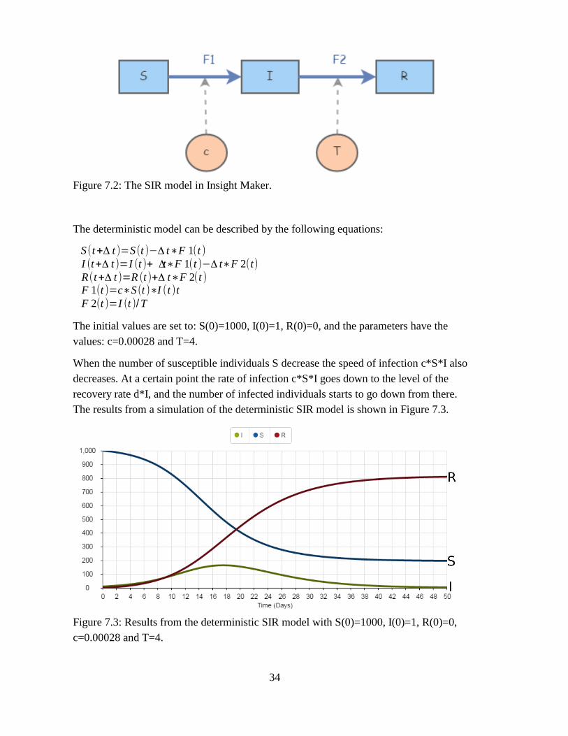
Figure 7.2: The SIR model in Insight Maker.

The deterministic model can be described by the following equations:

S(t+Δ t )=S(t )−Δ t∗F 1(t )I (t+Δ t )=I (t )+ Δt∗F 1(t )−Δ t∗F 2(t)R(t+Δ t )=R (t )+Δ t∗F 2(t )F 1(t )=c∗S(t )∗I (t )tF 2(t )=I (t )/T

The initial values are set to: S(0)=1000, I(0)=1, R(0)=0, and the parameters have the values: c=0.00028 and T=4.

When the number of susceptible individuals S decrease the speed of infection c*S*I also decreases. At a certain point the rate of infection c*S*I goes down to the level of the recovery rate d*I, and the number of infected individuals starts to go down from there. The results from a simulation of the deterministic SIR model is shown in Figure 7.3.

Figure 7.3: Results from the deterministic SIR model with S(0)=1000, I(0)=1, R(0)=0, c=0.00028 and T=4.

34

7.2.2 A stochastic SIR modelIn a deterministic SIR model with these specifications an epidemic always takes place. In real life, when only the first individual is infected, the disease can either die out or the disease can spread. This depends on whether the individual recovers before it infects othersusceptible individuals.

The deterministic model cannot take into account that the first infected individual might recover before spreading the disease to other individuals, but a stochastic model can take this into account. Their are two main events occurring in the SIR model: Individuals get infected and individuals recover.

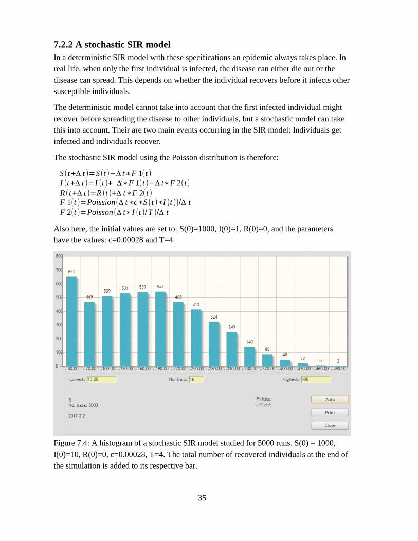
The stochastic SIR model using the Poisson distribution is therefore:

S(t+Δ t )=S(t )−Δ t∗F 1(t )I (t+Δ t )=I (t )+ Δt∗F 1(t )−Δ t∗F 2(t)R(t+Δ t )=R (t )+Δ t∗F 2(t )F 1(t )=Poission(Δ t∗c∗S(t )∗I (t ))/Δ tF 2(t )=Poisson(Δ t∗I (t )/T )/Δ t

Also here, the initial values are set to: S(0)=1000, I(0)=1, R(0)=0, and the parameters have the values: c=0.00028 and T=4.

Figure 7.4: A histogram of a stochastic SIR model studied for 5000 runs. S(0) = 1000, I(0)=10, R(0)=0, c=0.00028, T=4. The total number of recovered individuals at the end of the simulation is added to its respective bar.

35

The box plot feature

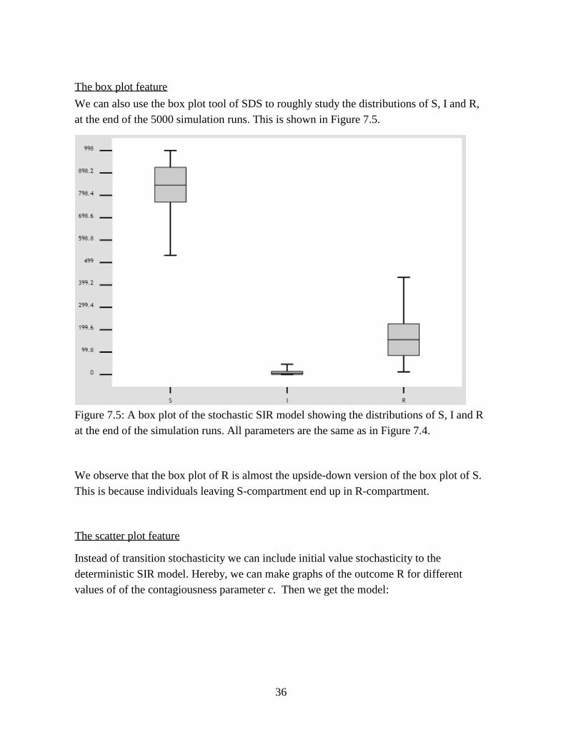
We can also use the box plot tool of SDS to roughly study the distributions of S, I and R, at the end of the 5000 simulation runs. This is shown in Figure 7.5.

Figure 7.5: A box plot of the stochastic SIR model showing the distributions of S, I and R at the end of the simulation runs. All parameters are the same as in Figure 7.4.

We observe that the box plot of R is almost the upside-down version of the box plot of S. This is because individuals leaving S-compartment end up in R-compartment.

The scatter plot feature

Instead of transition stochasticity we can include initial value stochasticity to the deterministic SIR model. Hereby, we can make graphs of the outcome R for different values of of the contagiousness parameter c. Then we get the model:

36

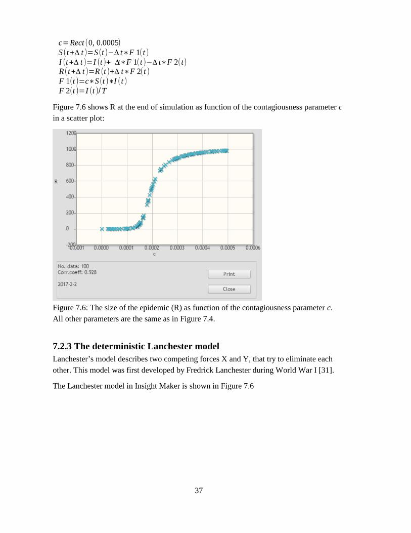
c=Rect (0, 0.0005)S(t+Δ t )=S(t )−Δ t∗F 1(t )I (t+Δ t )=I (t )+ Δt∗F 1(t )−Δ t∗F 2(t)R(t+Δ t )=R (t )+Δ t∗F 2(t )F 1(t )=c∗S(t )∗I (t )F 2(t )=I (t )/T

Figure 7.6 shows R at the end of simulation as function of the contagiousness parameter c in a scatter plot:

Figure 7.6: The size of the epidemic (R) as function of the contagiousness parameter c. All other parameters are the same as in Figure 7.4.

7.2.3 The deterministic Lanchester modelLanchester’s model describes two competing forces X and Y, that try to eliminate each other. This model was first developed by Fredrick Lanchester during World War I [31].

The Lanchester model in Insight Maker is shown in Figure 7.6

37

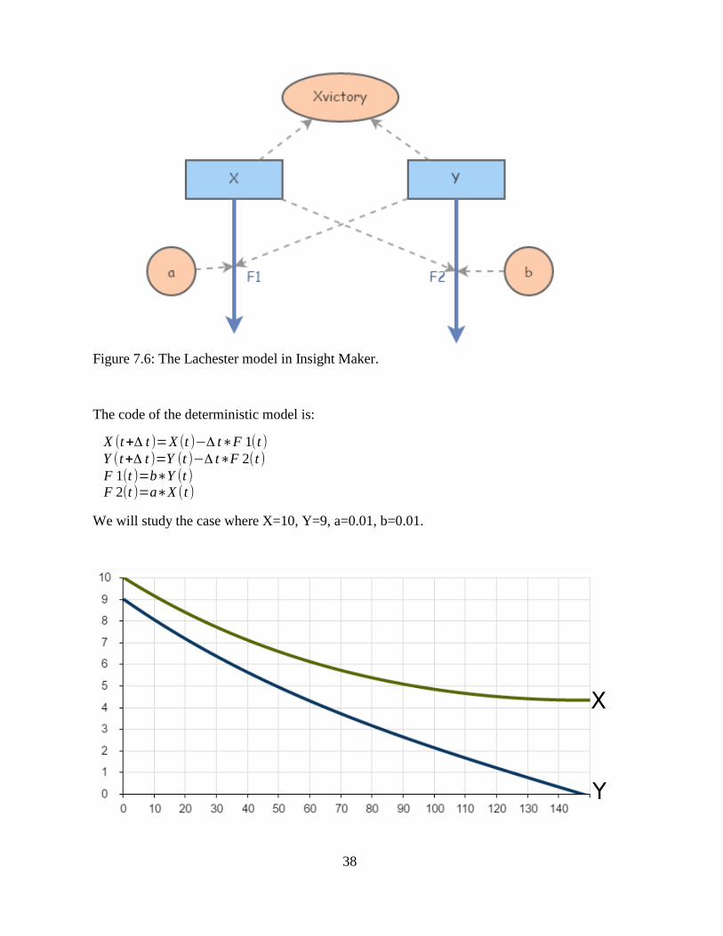
Figure 7.6: The Lachester model in Insight Maker.

The code of the deterministic model is:

X (t+Δ t )=X (t )−Δ t∗F 1(t )Y (t+Δ t )=Y (t )−Δ t∗F 2(t )F 1(t )=b∗Y (t )F 2(t )=a∗X (t )

We will study the case where X=10, Y=9, a=0.01, b=0.01.

38

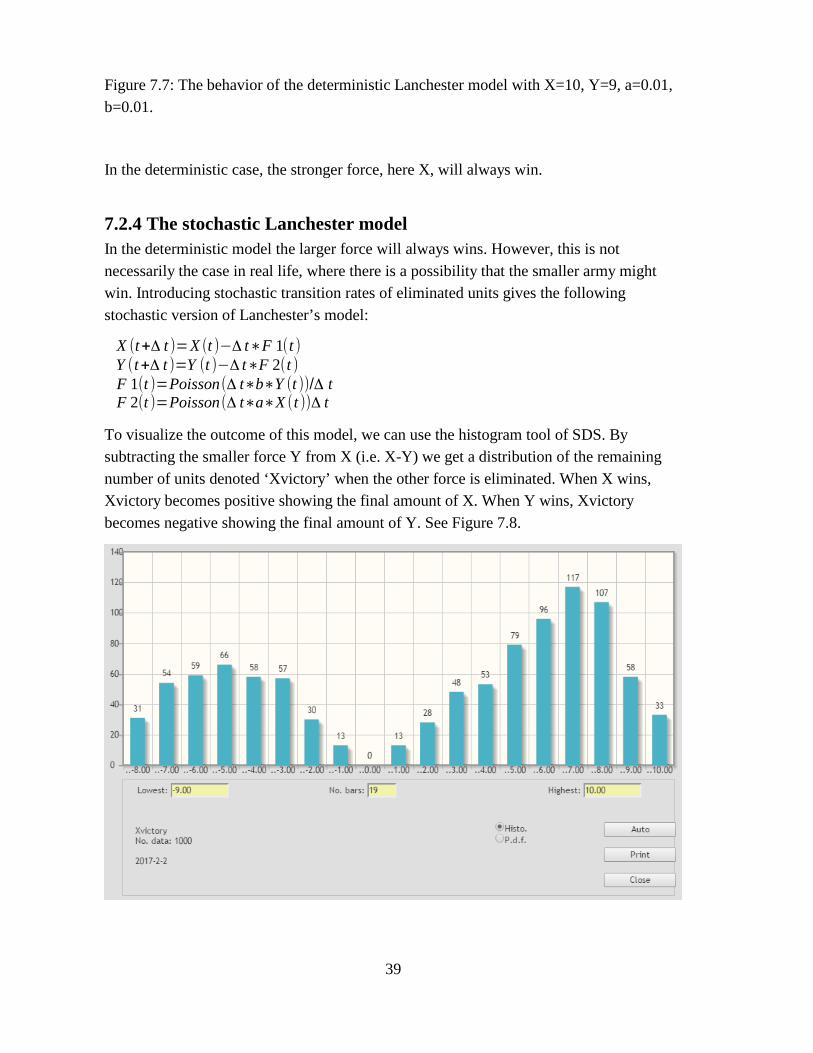
Figure 7.7: The behavior of the deterministic Lanchester model with X=10, Y=9, a=0.01, b=0.01.

In the deterministic case, the stronger force, here X, will always win.

7.2.4 The stochastic Lanchester modelIn the deterministic model the larger force will always wins. However, this is not necessarily the case in real life, where there is a possibility that the smaller army might win. Introducing stochastic transition rates of eliminated units gives the following stochastic version of Lanchester’s model:

X (t+Δ t )=X (t )−Δ t∗F 1(t )Y (t+Δ t )=Y (t )−Δ t∗F 2(t )F 1(t )=Poisson(Δ t∗b∗Y (t ))/Δ tF 2(t )=Poisson(Δ t∗a∗X (t ))Δ t

To visualize the outcome of this model, we can use the histogram tool of SDS. By subtracting the smaller force Y from X (i.e. X-Y) we get a distribution of the remaining number of units denoted ‘Xvictory’ when the other force is eliminated. When X wins, Xvictory becomes positive showing the final amount of X. When Y wins, Xvictory becomes negative showing the final amount of Y. See Figure 7.8.

39

Figure 7.8: A histogram of Xvictory for the stochastic Lanchester model with X=10, Y=9, a=0.01, b=0.01.

From this histogram we draw the conclusion that even Force Y might win, which could not happen in the deterministic case. We can also see from the shape of the histogram that small victories are rare, and that the winning side, no matter which, usually wins by a lot.

40

8 Discussion and conclusionsThe use of a stochastics System Dynamics model requires a large number of simulations to display the model’s behavior. Therefore, there is a need for a post analysis tool to statistically analyze the results. SDS is a tool aiming to fulfill this need.

Fulfillment of the project goals

The major goal of this thesis project was to create an open source tool for statistical analysis and presentation of the results from a stochastic model. In particular the tool should be able to display statistical estimates of averages, standard deviation, confidence interval, min max and percentiles of simulation results. Further it should be able to show distributions of a studied quantity, and also to calculate the correlation between different quantities. The tool created in this thesis project fulfills these project goals.

In addition to the specified goals we have also included a number of useful features such as:

• A device to control the seeds and thereby make a study reproducible.

• A feature to conditionally skip over irrelevant results based on a user defined condition.

• Export to an external file for analysis and presentation of the data with another software.

• Estimate of the remaining time of the session.

Evaluation of the statistical tool

The statistical tool has been thoroughly tested and evaluated. First, the correctness of the statistical calculation has been verified by simulations of different random number generators. Second, the tool has been tested against real stochastic models. Third, a significant amount of work was devoted to make the tool robust.

Planned use of this project

This project was performed to fulfill the need of stochastic modeling in epidemiology in ajoin project between Uppsala University and Karolinska Institute. It will also be used in courses in stochastic simulation at Karolinska Institute and at the Swedish University of Agricultural Sciences. However, we intend to make this tool universally accessible since SDS is a general tool that can be used in various fields.

41

Limitations and possible future work

Save and resume a session from file

Because statistics is generated by running an experiment a large number of times, it wouldbe useful if it was possible to save simulation session to a file and continue from where it ended in a later point in time. You cold then also take up the statistical analysis and presentation without new simulations.

Multi-dimensional presentation

SDS can currently not visualize multi-dimensional distributions. To overcome this limitation the current version of SDS already has an export feature which lets the user export data to another software where multi-dimensional visualization can be accomplished. Implementing ways to visualize multi-dimensional distributions inside of SDS could be a possible future work.

Compiled models

As discussed in section 4.4.3, the speed of the simulations was not a high priority goal when Insight Maker was created. Making improvements in this field would therefor be a possible future work. Insight Maker’s simulation engine that runs the models is currently interpretative as is most System Dynamics’ software. A potential future improvement could be to build a compiler for Insight Maker models that transform them into machine code. This would however be a large project, and possible a thesis work on its own.

42

9 References[1] L. Gustafsson and M. Sternad, “A guide to population modelling for simulation”, Open Journal of Modelling and Simulation, vol. 4, pp. 55-92, April 2016.

[2] J.W. Forrester, Principles of Systems. Cambridge, Mass, Wright-Allen Press: Inc. 1970.

[3] G.R. Richardson and A.L. Pugh III, Introduction to System Dynamics Modeling with DYNAMO, Cambridge, Ma: The MIT Press, 1981.

[4] J.L. Devore, Probability and Statistics for Engineering and Sciences, sixth edition, Toronto, Canada, Thomson Learning, Inc., 2004

[5] S.E. Alm and T. Britton, STOKASTIK – Sannolikhetsteori och statistikteori med tillämpningar, Stockholm, Sweden: Liber AB, 2008. (In Swedish)

[6] L. Gustafsson, “Poisson Simulation – A Method for Generating Stochastic Variations in Continuous System Simulation”, Simulation, vol. 74:5, pp. 264-274, 2000.

[7] D.T. Gillespie, “Approximate accelerated stochastic simulation of chemically reacting systems”, J. Chem. Phys. Vol. 115, pp. 1716-1733, 2001.

[8] L. Gustafsson and M. Sternad, “When can a deterministic model of a population system reveal what will happen on average?”, Mathematical Biosciences, vol. 243, pp. 28-45, 2013.

[9] J.W. Forrester, “The Beginning of System Dynamics”, M.I.T., July 13, 1989. Available: http://web.mit.edu/sysdyn/sd-intro/D-4165-1.pdf [Accessed: February 5, 2017].

[10] J.W. Forrester, Industrial Dynamics, Cambridge Ma: MIT Press, Cambridge, 1961.

[11] A.L. Pugh III, DYNAMO User’s Manual, including DYNAMO II/370, DYNAMO II/F,DYNAMO 111/370, DYNAMO III/F, DYNAMO III/F+, DYNAMO IV/370 and Gaming DYNAMO, Cambridge Ma: The M.I.T. Press, 1983.

[12] B. Richmond, Introduction to Systems Thinking, STELLA, Lebanon NH: High Performance Systems, Inc., 1992.

[13] Powersim Corporation, Powersim Reference Manual, Va: USA: Powersim Press, 1996.

[14] M. Sternad, “Utlysning av examensarbete”, Uppsala University, 2016 (in Swedish). Available: http://eglab.cc/doc/Utlyssning_exjobb.pdf [Accessed: February 5, 2017].

43

[15] S. Fortmann-Roe, “Insight Maker News May – June”, Insight Maker, 2014. Available: https://insightmaker.com/node/16484 [Accessed: February 5, 2017].

[16] The MathWorks, Inc., MATLAB: The language of Technical Computing, Natick, MA:The MathWorks, Inc., 1996.

[17] The MathWorks, Inc., “Simulink: Simulation and model based design”, Math Works, 2017. Available: https://www.mathworks.com/products/simulink.html [Accessed: February 5, 2017].

[18] Powersim AS, “Powersim Studio Products”, Powersim, February 2017. Available: http://www.powersim.com/main/products-services/powersim_products/ [Accessed: February 5, 2017].

[19] B. Blais, “Github - Python Numerical Dynamics Simulator”, Github, May 2015. Available: https://github.com/bblais/pyndamics [Accessed: February 5, 2017].

[20] VTT Technical Research Centre of Finland, “Simantics System Dynamics”, Simantics, 2014. Available: http://sysdyn.simantics.org/ [Accessed: February 5, 2017].

[21] ISEE Systems Inc., “Stella Architect”, ISEE Systems, 2017. Available: http://www.iseesystems.com/store/products/stella-architect.aspx [Accessed: February 5, 2017].

[22] S. Fortmann-Roe, “Insight Maker: A general-purpose tool for web-based modeling &simulation”, Simulation Modelling Practice and Theory, vol. 47, pp. 28–45, 2014.

[23] S. Fortmann-Roe, “Insight Maker API”, Insight Maker, 2013. Available: https://insightmaker.com/sites/default/files/API/ [Accessed: February 5, 2017].

[24] J. Korpela, “Tab Separated Values (TSV): a format for tabular data exchange”, Tampere University of Technology, September 2000. Available: http://www.cs.tut.fi/~jkorpela/TSV.html [Accessed: February 5, 2017].

[25] Joyent, Inc ., “Node.js Downloads”, Node.js, 2017. Available: https://nodejs.org/en/download/ [Accessed: February 5, 2017].

[26] M. Sopyło, “Introduction to HTML5 Desktop Apps With Node-Webkit”, Tutplus, December 2013. Available: https://code.tutsplus.com/tutorials/introduction-to-html5-desktop-apps-with-node-webkit —net-36296 [Accessed: February 5, 2017].

[27] T. Laurens, “How the V8 engine works?”, Github, April 2013. Available: http://thibaultlaurens.github.io/javascript/2013/04/29/how-the-v8-engine-works/ [Accessed: February 5, 2017].

44

[28] W.O. Kermack and A.G. McKendrick, “Contributions to the mathematical theory of epidemics”, Proc. Royal Soc., A 115, pp. 700-721, 1927.

[29] M. Braun, Differential Equations and Their Applications, New York: Springer-Verlag, 1993.

[30] D.G. Luenberger, Introduction to Dynamic Systems: Theory, Models and Applications, NY: John Wiley & Sons, Inc., 1979.

[31] F.W. Lanchester, Aircraft in Warfare, the Dawn of the Fourth Arm, London: Tiptree Constable and Co., Ltd., 1916.

45