Tax Reform under Fiscal Stress: A CGE Analysis of the Brazilian

Tax Reform.*

Victor Duarte Lledo

UNIVERSITY OF WISCONSIN- MADISON e-mail: vdlledo@students.wisc.edu

Resumo

Apesar do consenso acerca das distorções impostas pelo atual sistema tributário brasileiro, propostas de reforma na última década têm enfrentado várias restrições com relação a sua implementação. Duas destas restrições mostraram-se particularmente críticas: a) restrição de ajuste fiscal (a dívida do setor público não pode crescer), b) restrição do federalismo fiscal (receitas de estados e municípios não podem ser reduzidas). Este artigo procura analisar uma proposta de reforma que em princípio supera a restrição do federalismo fiscal. Usando o modelo desenvolvido por Auerbach and Kotlikoff (1987) calibrado para economia brasileira, eu procuro analisar os efeitos macroeconômicos de curto e longo prazo desta reforma, sujeita a restrição de ajuste fiscal. Analisa-se também os efeitos redistributivos desta reforma entre gerações com o objetivo de inferir a reação da opinião pública a sua implantação. A reforma consiste basicamente na substituição dos impostos indiretos sobre receitas operacionais do setor privado, os quais demonstram-se equivalentes a um imposto simétrico sobre a renda do trabalho e do capital, por um novo imposto sobre o valor adicionado (VAT) federal. Simulações desta reforma apresentaram efeitos macroeconomicos positivos tanto no curto como no longo prazo. Apesar de uma elevação substancial na taxa média do novo VAT nos primeiros anos após a reforma, a maioria das gerações apresentaram um aumento de bem-estar ao longo da vida, tornando-se potencialmente em favor da reforma. Palavras Chaves: reforma tributária, federalismo fiscal, equilíbrio geral computável, Brasil.

Abstract

In spite of a general agreement over the distortion imposed by the current Brazilian tax system, attempts to reform it during the last decade have faced several restrictions to its implementation. Two of these restrictions were particular binding: a) fiscal adjustment restriction (public sector debt cannot increase), b) fiscal federalist restriction (revenues from individual states and municipalities cannot decrease). This paper focuses on a specific reform that overcomes in principle the fiscal federalist restriction. Using Auerbach and Kotlikoff (1987) model calibrated for the Brazilian economy, I analyze the short and long run macroeconomic effects of this reform subject to the fiscal adjustment restriction. Finally, I look at the redistributive effects of this reform among generations as a way to infer about public opinion’s reaction to the reform. The reform consists basically of replacing indirect taxes on corporate revenues, which I show to be equivalent to a symmetric tax on labor and capital income, by a new federal VAT. The reform presented positive macroeconomic effects both in the short and long run. Despite a substantial increase in the average VAT rate in the first years after the reform, a majority of cohorts experienced an increase in their lifetime welfare, being potentially in favour of the reform.

Keywords: tax reform, fiscal federalism, computable general equilibrium, Brazil JEL: C68, E60, H20, H77 Área de Interesse SBE : Macroeconomia Aplicada * Artigo submetido ao XXIII Encontro Brasileiro de Econometria a se realizar entre 12 e 14 de dezembro de 2001 em Salvador, Bahia.

2

I. Introduction By briefly reviewing the political process behind the Brazilian tax reform in the last ten years, it is possible to recognize two major restrictions different tax reform proposals have always faced: (i) a fiscal federalist restriction, which basically states that revenues from individual states and municipalities cannot substantially decrease, and (ii) a fiscal adjustment restriction, which consists of the imposition that the debt of the consolidated public sector (direct administration of the federal, state and local governments plus state enterprises and autarchies) cannot increase. The need to control the overall level of debt by increasing tax revenues, while diverting part of those revenues to pay for the debt service under a limited margin to reduce public expenditures as well as to reduce tax revenues available for states and municipalities, characterizes the fiscal stress condition the Brazilian public sector has been experiencing specially in the last six years of President Cardoso’s mandate.

The main objective of this paper is to evaluate the macroeconomic and redistributive effects of a reform capable of overcoming the fiscal stress conditions. My strategy was to limit the search to tax reform proposals already debated inside the Brazilian Congress which at the same time did not change revenue-sharing agreements as well as the intergovernmental assignment of important subnational taxes. In doing that I set aside the fiscal federalist restriction focusing on the ability of the reform in respecting the fiscal adjustment constraint.

The tax reform proposed consists basically of replacing the so-called cumulative taxes, which are federal indirect business taxes on corporate sales by a new federal VAT whose revenues are not shared either with states or with municipalities. Since taxes on corporate sales can be shown to be equivalent to a symmetric tax on labor and capital income, this reform can also be interpreted as a partial switch to a consumption tax system. The macroeconomic and redistributive effects of this proposed tax reform are simulated with the help of Auerbach and Kotlikoff (1987) overlapping generation (OLG) dynamic computable general equilibrium (CGE) model and algorithm, hereafter referred to as the A-K model. Araujo and Ferreira (1999) is, to the best of my knowledge, the only analysis that has used a dynamic geral equilibrium model to simulate the effects of the Brazilian tax reform. In a model with infinitely lived individuals they simulate the effects of two different tax reform proposals submitted to the Brazilian Congress. Both reforms delivered long-run growth and welfare effects.1 My analysis differs from theirs in two important dimensions. Instead of looking at the effects of a comprehensive set of fundamental reforms in the tax system, by the reasons already presented, the focus here will be on a particular subset of such reforms. Moreover, by using an overlapping generation model, my analysis will try to incorporate the distributive effects of the tax reform.2 While their focus was mostly on identifying the efficiency of different tax reform proposals, mine is more on the implementability of proposals whose positive macroeconomics effects have been consensually acknowledged. Analyses of the implementability of the Brazilian tax reform proposals have already been conducted by Werneck (2000). Werneck defines a system of equations relating tax revenues available to each government level in Brazil as a function of the size of their assigned statutory bases and their respective tax rates along with parameters measuring each

1Their results are in tune with the CGE literature based on infinitely-lived representative agent models (see Lucas (1990), King and Rebelo (1990), Jones, Manuelli and Rossi (1993), Stokey and Rebelo (1995), Cassou and Lansing (1996)), which revealed the efficiency and growth effects of dropping income taxes for the US tax system 2 The incorporation of intergenerational and intragenerational heterogeneity in CGE models has sometimes disputed the results obtained in representative agent models (see Krussel, Quadrini and Rios-Rull (1996)) and, in general, made explicit that while there may be positive growth effects from eliminating income taxes they are not appropriated by all individuals (see Auerbach and Kotlikoff (1987) and Auerbach et al (2001)).

3

government level productivity in the collection of such taxes. This model is used to simulate the effects of the 1997 tax reform proposal submitted to Congress by the Executive branch of the Federal Government on the level and allocation of revenues among different government spheres.3 This paper extends Werneck (2000) by using the more structural approach developed in the A-K model to look at the dynamic effects of tax reform subject to the fiscal stress conditions described above. It also attempts to measure public opinion’s reaction to the reform through the computation of the remaining lifetime utility concept introduced in Auerbach and Kotlikoff (1987). The remainder of this paper is organized as follows. Next section presents a general background on the Brazilian tax reform, identifying the sources of distortion in the Brazilian tax system along with the main obstacles different proposals faced towards their implementation. The A-K model used to simulate the reform is presented in section III. Section IV documents the parameterization and calibration procedures. Section V presents the simulation results. Main conclusions are summarized in section VI. Two appendixes are found at the end of the manuscript. The first collects the tables and figures used to illustrate the analysis. The second presents the equivalence between corporate and household taxes under the A-K model. II. A Background on the Brazilian Tax Reform. A. The Brazilian Tax System: Changes and Effects. The current Brazilian tax system was implemented in the 1988 Constitutional reform inheriting its basic features regarding the assignment of tax bases and tax revenues among government levels from the previous 1967 Constitution.4 While there has been isolated and repeated changes in specific aspects of the legislation that regulates the Brazilian tax code since then, both the nature of tax reform proposals as well as the obstacles to their implementation owe most of their origins to two fundamental changes in the tax system.

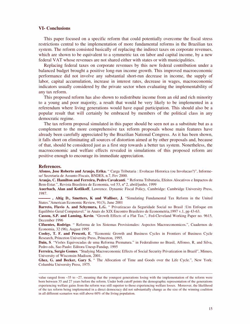
Figure 1 gives you a general idea of the Brazilian tax system by contrasting the evolution of the tax burden after the 1967 and 1988 constitutional reforms with the participation of indirect taxes in the total burden. Indirect taxes comprising business taxes on corporate sales and value-added taxes accounted for the majority of the burden right after the 1967 reform. 5

The period that followed the implementation of the 1967 tax system until the implementation of the 1988 tax system was marked by a decline in the participation of indirect taxes accompanied by a stable tax burden around 25% of GDP. The period following the 1988 constitutional reform, on the other hand, brought a substantial increase in the participation of indirect taxes. That happened along with a more volatile but clearly increasing total tax burden, which more recently has reached historically high levels above 30% of GDP.

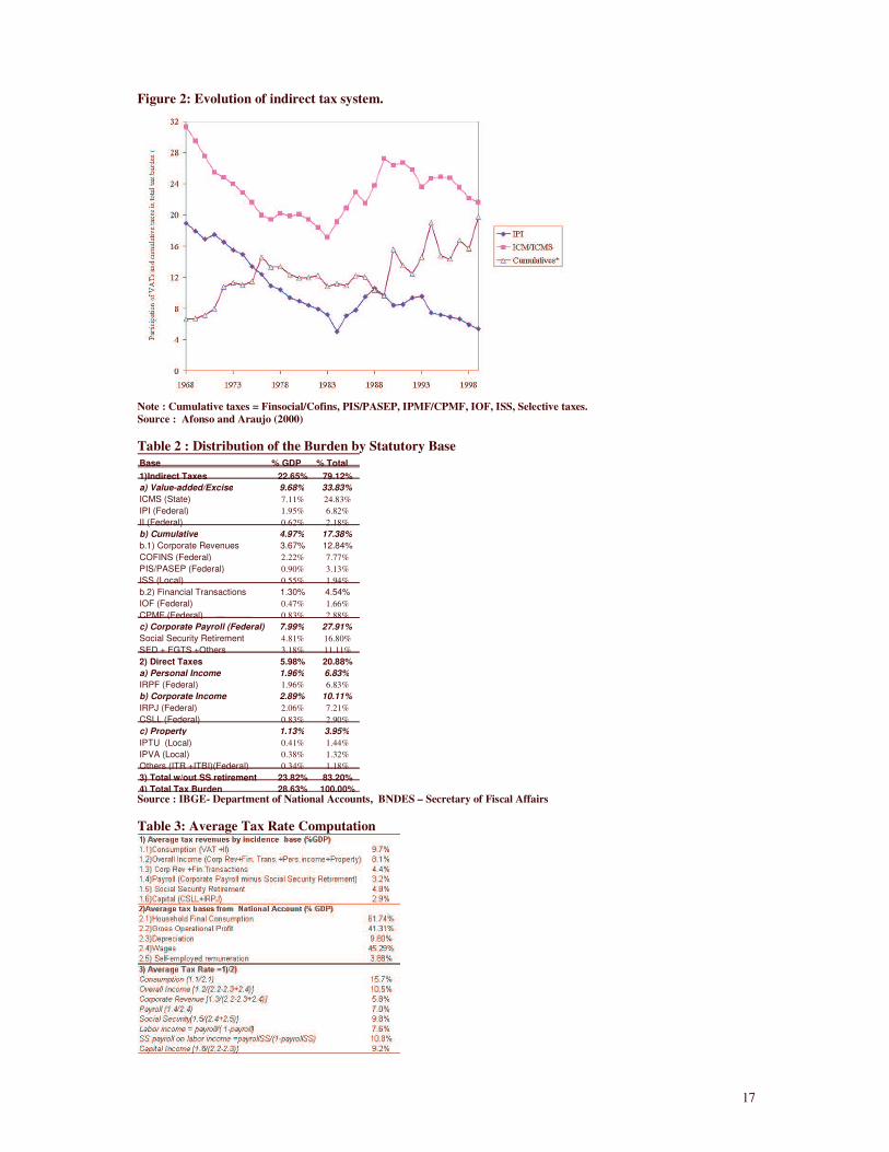
However, it was not so much the strong reliance on indirect taxes but their cumulative nature that has been one of the main sources of criticisms of the current tax system. Figure 2 3 Werneck is interested in finding combinations of tax rate and tax base size parameters capable of leaving revenues of different government levels unaltered. He is particularly interested in exploring the trade-off between the broadness of the tax base and the size of the tax rate required by the new tax system in order to comply with the fiscal stress restrictions. 4 Two features of the Brazilian tax system have assumed central stage in the current tax reform debate: the dual VAT system and the revenue sharing system. The 1967 Constitution introduced a dual VAT system where central and state governments where granted the autonomy to administer two distinct value-added taxes (VATs). A VAT over manufactured products (IPI) was assigned to the central government while another VAT (ICM) on sales of non-manufactured goods and services. More on the revenue sharing system below. 5 Due to their cascading effects where the same tax is paid more than once throughout the productive chain, those indirect business taxes are often referred to as cumulative taxes. They correspond to the following taxes: Finsocial/Cofins, PIS/PASEP, IPMF/CPMF, IOF, ISS. COFINS and PIS/PASEP are both taxes on corporate revenues whose proceeds were originally designed to complement the social security budget. IOF and IPMF/CPMF could be crudely defined ash taxes over financial transactions. ISS is also a tax on revenues from services. With the exception of the IPMF/CPMF, which was created more recently, and the ISS assigned to local governments, all these taxes were created during the seventies and assigned to the central government

4

illustrates this point by contrasting evolution of the federal and state VAT burden Vis a Vis the burden of the remaining cumulative indirect taxes. After 1988 we can simultaneously observe a steady decrease in the participation of the federal VAT (IPI) in the overall tax burden followed by a substantial increase in the tax burden of the remaining cumulative indirect taxes (Finsocial/COFINS, PIS/PASEP, IPMF/CPMF, ISS and IOF).

The burden of those cumulative taxes was relatively small and stable up until 1988 when a increasing trend led it to more than double its participation in the total tax burden. This increasing reliance on cumulative taxes emerged as the federal government reaction to the changes in the new revenue sharing system coupled with the increasing external and internal pressure for fiscal adjustment.

Without changing the essence of the revenue sharing system originated in 1967, the 1988 reform substantially increased the share of tax revenue raised by the central government that had to be transferred to state and municipalities. It also increased the transfers of state tax revenues to municipalities. The bulk of federal transfers to state and municipalities had their proceeds from a fund that retained 14.5% of the revenues on VATs and income taxes in 1967. This amount was raised to 21.5% in 1988 (almost 30% if you include transfers from regional funds with the same sources). The share of the state VAT transferred to municipalities, as shown in Table 2, has also increased from 20% to 25% after 1988.

The decentralization of tax revenues, which had begun with the redemocratization period a few years before, was celebrated as one of the high points of a longer process of devolution of political and fiscal power to state and municipalities. It came, however, in a period of increasing inflationary pressures. Eliminating and controlling inflation would demand a strong fiscal adjustment from the overall public sector and especially from the central government that was liable for most of the public debt.

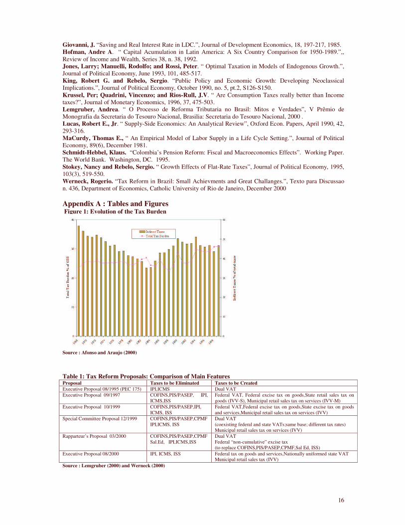
With the pressure of fiscal adjustment on one side and little space to fully explore its value-added and income taxes on the other, the central government had to rely on the taxation of non-shared tax bases, basically cumulative taxes, in order to increase revenues. That was done by increasing the tax rates of COFINS and PIS/PASEP in conjunction with the creation of IPMF later renamed CPMF. B. Identifying and overcoming obstacles to tax reform implementation. The distortions stemming from the 1988 Constitution led to the elaboration of several tax reform proposals just a few years after its promulgation. Last decade was marked by a continuos debate on how to reform the tax system in order to eliminate some of these distortions. This debate has presented two important characteristics: (i) the recognition of the indirect tax system as the main source of distortion in the Brazilian tax system, (ii) the central role of Federal and state government positions manifested in the majority of tax reform proposals submitted to the National Congress. 6 Table 1 contrasts the six tax reform proposals, which have assumed center stage in the Brazilian tax reform debate since 1995. The Federal government position in the debate, strongly defended by the Ministry of Finance, consisted of the imposition that the proposed tax reform could not compromise even in the short-run the tax effort required by the overall public sector in order to eliminate structural public deficits and stabilize the net debt of the public sector. Complying with this fiscal adjustment restriction was recognized as an important fundament to the sustainability of the stabilization program implemented in 1994 (Real Plan).

6 Lemgruber (2000) and Werneck (2000) present a descriptive and critical appraisal of the political process behind the debate of each of the tax reform proposals. Dain (1995) describes in more depth earlier proposals submitted by non-governmental groups.

5

The second position defended by subnational elected officials and defined as the fiscal federalist restriction consisted of the imposition that the tax reform could not compromise neither the disposable revenues available to states and municipalities nor the enhanced tax autonomy those members of the federation acquired after the 1988 tax reform. The same process of political and fiscal decentralization that shifted to states and municipalities the responsibility over the provision of important goods and services also shifted to state and local residents the power to control the quality of those services through the electoral system. State and municipal elected officials, zealous of their political careers, started opposing any fundamental change in the system of intergovernmental transfers or in the assignment of tax bases that would put in risk their flow of disposable revenues.

The fiscal adjustment restriction was particularly binding to the elimination of the federal cumulative taxes, due to the uncertainty to whether the new federal taxes would be able to match the revenue-raising ability and administrative efficiency of the current system. It became even critical as the reliance of the federal government on those revenue sources continuously increased in the last decade, as it was already illustrated in Figure 2. COFINS and PIS-PASEP, two of the most important federal social contributions accounted for almost 10% of total tax burden between 1994 and 1998 as shown in Table 2.

The fiscal federalist restriction, on the other hand, has been crucial to the debate over the assignment of the VAT among different government levels, the principle to be used in its collection and the rules regarding the vertical and horizontal distribution of its revenues. Behind this debate was also the uncertainty about the level of revenues available to different states and municipalities after the reform. The state VAT (ICMS), an object of reform in all the proposed reforms, has been consistently the most important source of revenue for states in the last thirty years amount to more than 20% of all revenue collected (see Table 2).

The inability to reform the Brazilian tax system in the past ten years, despite an almost consensual recognition of the distortions imposed on the private sector, is a reflex of the wide array of interests affected by different proposals. In trying to deal simultaneously with the elimination of cumulative taxes and with the complete redesign of the consumption tax system is not surprising that the several tax reform proposals discussed in the past ten years have been facing so many obstacles to their implementation.

A more recent trend in the debate about tax reform seems to be recognizing the shortcomings of a comprehensive reform and the option for dealing with isolated points of the reform in stages. The analysis in this paper represents an initial attempt to explore this venue by analyzing the effects of replacing the cumulative taxes assigned to the federal level (COFINS, PIS-PASEP, CPMF and IOF) by a new federal VAT whose proceeds are not shared with subnational governments. The idea of replacing cumulative taxes on corporate revenues by a federal VAT has been part of the 1997 and 1999 tax reform proposals defended by the Executive. It has also been present in the proposal approved by the Legislative Special Committee. Its omission both from the 2000 non-voted Rapporteur’s proposal and from the latest proposal presented by the Executive exemplifies the increase role of the fiscal adjustment restriciton to the advance of the Brazilian indirect tax system. This reform will not modify the current dual VAT system. Neither will it touch on the 1988 intergovernmental revenue-sharing agreements. Therefore, the amount of disposable revenues to subnational governments will not be altered. With the fiscal federalist restriction not being binding, the implementation of this proposal will depend on whether there are still positive macroeconomic and welfare gains from this reform even after the imposition of a fiscal adjustment restriction. The rest of the paper quantifies this analysis using a dynamic CGE model calibrated for the Brazilian economy.

6

III. The Model. The model used in the tax reform simulations below was developed in Auerbach and Kotlikoff (1987). It is an overlapping generation (OLG) model where all agents live for 55 periods. At any point in time the economy is populated by 55 different cohorts. Within each cohort individuals are identical. Heterogeneity arises only between different cohorts and corresponds to differences in earning abilities or in human capital levels- et. Population growth is exogenous at the rate η. A. Preferences and the Household Budget Constraint. Household preferences are represented by a utility function with current and future values of consumption and leisure as arguments presented in (1). They are restricted to be time-separable and of the nested, constant elasticity of substitution (CES) form which means that the annual utility function takes the form in (2). Moreover, the annual utility function does not change with time - (.).(.) uut ≡ )],(),...,,([),( 555555111 lculcuUlcU = . (1),

)/11/(1)/11()/11( ][ ρρρ α −−− += ttt lcu . (2) Thus, each household begins her economic life at date t chooses a perfect-foresight consumption path (c), leisure path (l), leaving no bequests and receiving no inheritances in order to maximize a lifetime utility function of the following form.

U c ltt

tt t=

−+ +− −

=

− − −

�1

11

1 1

1

55 11

11

11

γ

δ αρ ρ γ( ) [ ]( )( ) ( ) ( )

(3)

In (3) ρ is the intratemporal elasticity of substitution between c and l. It determines how responsive an individual’s annual labor supply is to the wage rate in a given year. α represents the utility weight on leisure. The greater is α, the less labor the household will supply in order to obtain consumption goods. The parameter δ is a discount rate, which signals the degree of preferences of different bundles (l, c), across time. The larger is δ, the larger the fraction of lifetime resources a household will spend earlier in her life. The remaining taste parameter, γ, corresponds to the household’s intratemporal elasticity of substitution between consumption in different years. The size of γ determines the responsiveness of households to changes in the incentive to save. The optimal path of consumption and leisure is subject to a lifetime balanced budget constraint, which requires the present value of her lifetime consumption to be smaller or equal to her after tax lifetime income. This constraint can be written as:

[ ( )] [ ( )( ) ( ) ]1 1 1 1 1 011

551+ − − − − − + + ≥

==

−∏� r w e l c PVBss

t

tkt t t t lt st ct tτ τ τ τ (4)

Where rt is the interest rate in period t, wt is the standardized wage rate in year t and et is the level of human capital referred to in the beginning of the section. τk, τl and τc are the marginal tax rates imposed on capital income, wage income and on consumption, respectively.

7

Individuals also contribute to a pay-as-you-go social security system (PAYG) through a tax on corporate payroll (τs) expecting to receive an amount PVB in lifetime social security benefits.7 Each individual’s labor supply decision is also constrained to be nonnegative. If the household would choose to demand more than one unit of leisure in a given period, the individual must “retire” for that year. Equation (5) below presents this constraint.

lt ≤1 for all t (5)

B. Technology. The model has a single production sector. Output is produced by identical

competitive firms using a neoclassical, constant-returns-to-scale production technology. Capital is assumed to be homogeneous and non-depreciating, while labor differs only in its efficiency.

The aggregate production technology is the standard Cobb-Douglas form. Y K Lt t t= −θ θ1

(6) Where Yt is aggregate output, A is the exogenous technological constant and θ is

capital’s share in production. Capital is owned by individuals and supplied every period to firms along with labor.

This assumption reduces firms’ optimal decisions to a simple problem of renting capital and hiring labor in order to maximize profits taking given wages and interest rates, as input markets are also assumed to be competitive.

Competitive pre-tax wages and interest rates are thus given by the marginal product of labor and capital, respectively.

rt= θ (Kt/Lt) θ -1 (7a), wt= (1-θ)(Kt/Lt)θ (7b)

C. Government. At any time t, the government collects tax revenues (Tt) and issues debt (Dt+1) which is used to finance government purchases of goods and services (Gt) and interest payments on the inherited stock of debt (Dt). This relationship is expressed in equation (8) below. Dt+1- Dt + Tt = Gt +rtDt (8) Revenue is raised with the imposition of proportional taxes on consumption, labor and capital income as expressed in (9) Tt = (wt –et)(1-lt) τlt + τctct +τktrtKt (9) The level of government expenditures in the initial steady state, G*, is determined endogenously in order to satisfy the balanced budget requirement in this period .8 It is held fixed at its steady-state value throughout the transition path (Gt=G*).

Recursive substitution of the expression (8) into itself for time periods 0 to N yields ])]1(1[])]1(1[[])]1(1[[ 1

00

1

0 0

1

0 0Nkts

N

ttks

t

t

sstks

t

t

ss DrDGrTr −

=

−∞

= =

−∞

= =

−+−+−+=−+ ∏� ∏� ∏ τττ (10)

In the long run, as N → ∞ , the last term goes to zero by a non- Ponzi Game

restriction. Equation (10) can be rewritten as follows

01

0 0

1

0 0

])]1(1[[])]1(1[[ DGrTr tkst

t

sstks

t

t

ss +−+=−+ −

∞

= =

−∞

= =� ∏� ∏ ττ (11)

7 Even tough none of the tax reform experiments will involve modifications in the social security system; its inclusion is justified on the basis that it presents an additional burden in the tax system, which needs to be taken into consideration before tax reform experiments are implemented. 8 In steady-state Dt+1=Dt= D*,Tt =Tt+1=T*, rt=rt+1=r* what implies that Gt=Gt+1 =G*=T*+ r*D*.

8

IV. Parameterization and Calibration.

In order for the model presented in the previous section to generate a numerical equilibrium, we need to specify specific values for its fiscal, demographic, technology and preference parameters. Such parameters, whenever possible, were estimated using Brazilian data.

The time-constrained reader can jump this section and go straight to Table 4 and 5. Table 4 collects the parameters ultimately used in the benchmark equilibrium along with the others previously calculated or imputed. Table 5 contrasts the simulated variables in the initial steady state with those observed in real Brazilian economy.

The remainder of this section discusses in more detail the imputation of values for different parameters in the model along with the calibration of its initial steady-state.

A. Tax rates The A-K model presented above, albeit rich in several dimensions, does not include a corporate tax structure. Only household taxes on consumption, labor and capital are allowed in the model. Therefore, before calibrating the model, one needs to “convert” corporate tax rates into household tax rates on consumption, labor or capital income. The assumptions and steps required to establish this conversion are presented in detail in the Appendix. Having that in mind, we have used a set of proportional tax rates on consumption, capital and labor income along with an average payroll tax to approximate the average burden between 1994 and 1998 of the Brazilian (federal, state and local) tax and social security system. Table 2 organizes the distribution of the tax burden by statutory base. The calculation of each of the average tax rates presented below is based on this being summarized on Table 3. The overall burden on consumption was computed by dividing the average between 1994 and 1998 of all tax revenues from all value-added and excises taxes charged at the federal, state and local level over the same period of time.9 The result was an average consumption tax rate (τc) of 15.7%. An average tax rate on labor income taxation was computed in two stages. In the first stage an average tax on corporate payroll was computed by dividing the 1994-98 average tax revenue from all federal taxes and social contributions on corporate payroll not used to finance retirement pensions in the social security system by aggregate corporate payroll during the same period. 10 The resulting average tax rate was 7%. In the second stage, we used the formula derived in the Appendix to convert corporate payroll taxes into household wage income taxes leading to an average tax on labor income of 7.6%. The social security payroll tax used to finance retirement pensions of the social security system was computed by dividing the 1994-1998 average revenue from this contribution (Social Security retirement on Table 3) by the total wage earnings received by employed (aggregate corporate payroll) and self-employed workers. The tax base for the social security payroll tax differs from the base from other payroll taxes by the inclusion of aggregate earnings from self-employed workers over which social security taxes also incides. The resulting tax rate (τs) is 10.8%. Given the equivalence between taxes on corporate profits and capital income presented in the Appendix, an average tax rate on capital income was calculated by dividing the 1994-98 average revenues from the federal IRPJ and CSLL, only taxes on corporate profits, by aggregate corporate profits. On its turn, aggregate profits were computed by

9 Implicitly on this computation was the equivalence between VAT and a tax on the consumption of final goods, a standard result in the literature. VATs: IPI, ICMS. Excise taxes: II. 10 Corporate payroll taxes: FGTS, Salário educação (SED), others.

9

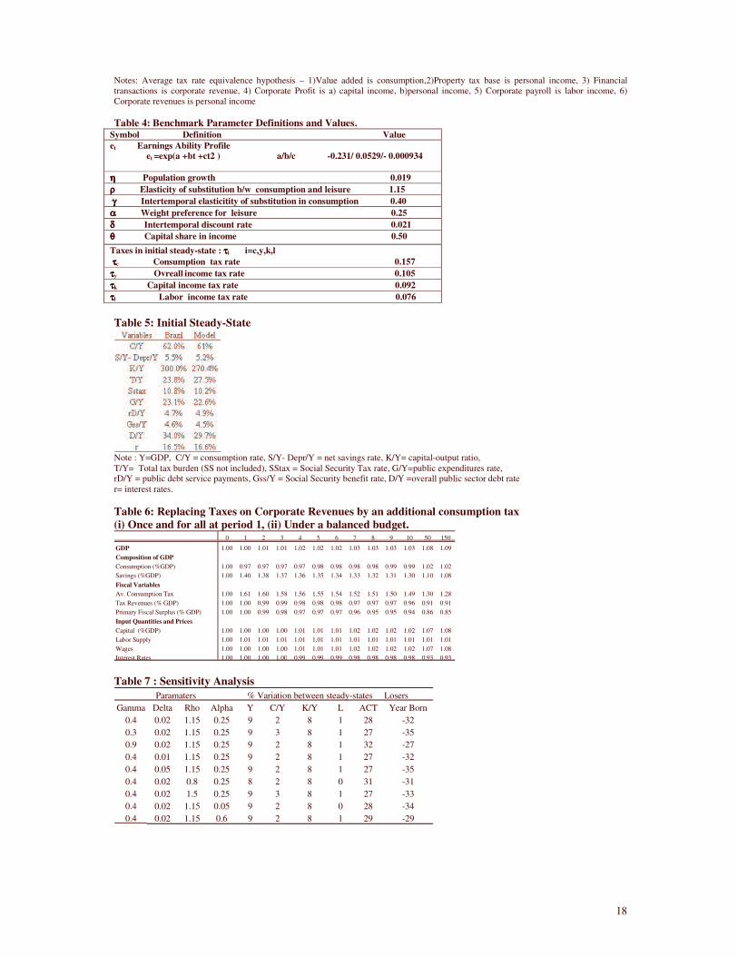
subtracting the total depreciation from the aggregate gross operational surplus. The result was a 9.2% average tax rate on capital income. The total burden on income is finally computed with the calculation of a tax rate on overall income. This tax rate tries to capture the burden of taxes whose effective base is neither labor nor capital income but some combination of both. We have included in this group federal personal income taxes (IRPF); federal, state and local taxes on residential and commercial property (IPTU, ITR) and state taxes on automobile property (IPVA). We have also included in this group taxes on corporate revenues (COFINS, PIS/PASEP, IOF, CPMF) which, as shown in the Appendix, are equivalent to a symmetric tax on labor and capital income.11 The average tax on overall household income was obtained after dividing the average revenues between 1994 and 1998 from all taxes above by the after tax net domestic income, defined as the remuneration of employed and self-employed workers (wages) plus gross operational surplus (gross profits) minus total depreciation. The result is an average tax on overall income equal to 10.5 % leading to effective average tax rate on labor (τl) and capital (τk) equal to 18.1% and 19.7%, respectively. B. Demographics: Population Growth rate and Earnings-Ability Profile. Population growth (η) was set equal to 1.9%, its historical average up until 1998. An individual’s earning ability or human capital profile is an exogenous and stationary function of her age. Auerbach and Kotlikoff (1987) have parameterized this profile as an exponential function of years of experience and its square: et = exp ( a + bt +ct2) (13) Having this functional form specification as the starting point, Ferreira (2001) estimates the returns on experience for urban male workers between 25 and 65 years old using the Brazilian Survey of Household Samples (PNAD). After controlling for time, geographical and school level effects, he obtains estimates for a, b and c respectively equal to –0.231, 0.05 and –0.0009, which were used in this calibration. C. Technology and Preference parameters The parameter θ in the Cobb-Douglas represents the participation of capital in national income. This can be easily derived by realizing from (6) that Y/K equals (Kt/Lt) θ

which reduces (7a) to: rt= θ Y/K (7a’) θ is obtained through the multiplication of the interest rate by the capital-output

ratio.12. Using an average yearly interest rate between 1994-98 of 16.54% leads to a θ approximately equal to 50% (49.62%).13

The parameterization of preferences is much more controversial given the absence of good data and consequently of a systematic attempt in order to estimate such parameters for the Brazilian case. There has been no empirical study trying to estimate the intertemporal elasticity of substitution (γ) for Brazil.14 The same problem is also observed with respect to

11 IOF and CPMF statutory base is financial transactions. We have assumed, however, that the majority of such transactions are conducted by firms, leading us to consider those taxes equivalent to taxes on corporate revenues. 12 A capital-output ratio for the Brazilian economy was estimated by Hoffman (1992) and Araujo and Ferreira (1999). Using different metrologies and time-series both papers found a capital-output ratio approximately equal to 3 13Araujo and Ferreira (1999), Barreto and Schymura (2000) and Ferreira (2001) have also used the same value in their respective analysis. 14 There has been, on the other hand, some attempt in order to estimate this parameter for other developing countries. Values for γ range between 0.5 (Giovanni 1985) and 1 (Schmidt-Hebbel 1994). The estimates of � tend to be in the range between 0.10 and 0.45 for developed economies and in studies that accounted for both leisure and consumption (MaCurdy 1981).

10

the intratemporal elasticity of substitution between consumption and leisure (ρ) and the intratemporal weight preference for leisure.15 Some effort was made in order to calculate a Brazilian estimate for the intertemporal discount rate. Araujo and Ferreira (1999) estimated a δ approximately equal to 0.07. 16 This value is higher than the estimate of 0.03 found for Colombia (Schmidt-Hebbel 1994) as well as than the estimate of 0.02 obtained for Chile (Cifuentes 1993). For the U.S. economy, recent estimates have ranged between 0.01 (McGrattan 1994) and 0.06 (Cooley and Prescott 1995).

D. Benchmark Equilibrium and Calibration The model presented in the previous section was calibrated to match an average between 1994 and 1998, the most recent year for which reliable macroeconomic aggregates can be found. The average between 1994 and 1998 was chosen because 1998 was a very unstable year due to the international financial crisis that followed the Russian debt default and that ultimately led Brazil to adopt a flexible exchange rate regime in the beginning of 1999. Financial and fiscal variables were specially affected by the crisis. The real macroeconomic variables selected were those commonly used in CGE analysis. Besides the capital-output ratio (K/Y) already mentioned, two other real macroeconomic variables were selected: the household consumption rate and the net national saving rate.17 A group of fiscal aggregates was also calculated to be part of our benchmark equilibrium. Total tax revenues amounted 28.6% of GDP between 1994-98 of which 23.79% were collected through taxes administered by federal, state and local governments and the remaining 4.81% were collected through social security contributions used to finance retirement pensions.18 Government expenditure of the consolidated public sector, which includes the direct administration of federal, state and local governments along with state enterprises, the central bank and the social security system accounted on average for 27.6% of GDP between 1994-1998 out of which retirement benefits distributed by the social security system represented approximately 5% of GDP. The difference between total expenditures and revenues- primary deficit- was actually negative corresponding to a surplus of 1% of GDP. After including the servicing of debt- approximately 5% of GDP- the primary surplus became an operational deficit of almost 4% of GDP.19 One last variable used in our benchmark equilibrium was the real interest rate. Our measure for the real interest rate was the TJLP (long-run interest rate) fixed by the Brazilian Central Bank. The average between 1994-1998 was 16.5%.

Having the average tax rate, the technology and demographic parameters fixed at the values previously estimated, the calibration of the initial steady-state consisted in using 15 A ρ equal to 0.83 estimated in Ghez and Becker (1975) is one of the few references cited. Auerbach and Kotlikoff (1987) make no mention of any estimate for α. 16 Their intertemporal discount rate was actually equivalent to 1/1+δ and, hence, equal to 0.93 17The household consumption rate (C/Y), defined simply as the share of GDP consumed by families has been very stable over the last fifty-years and the rate of 62% was not so different from this historical trend. The net national saving rate averaged between 1994-1998 was equal to 5.5%. It was computed by subtracting from the gross savings rate- 19% of GDP- foreign savings in the amount of 3% of GDP and the depreciation of physical capital estimated to be around 10.5% of GDP. The value of 10.5% of GDP was obtained by multiplying an estimated depreciation rate of 3.5% of the stock of capital by the capital-output ratio of 3. 18 Table 2 used to compute average tax rates shows the components of the total tax revenue in more detail. 19 Another important fiscal aggregate calculated for the initial benchmark equilibrium was the consolidated public sector net debt whose average between 1994-98 was 34% of GDP. This variable was not only an important referential in the calibration of the benchmark equilibrium but also an important input in the computation of the debt ratio. This variable, defined, as the ratio between the aggregate public debt and the capital stock is an important parameter required by the algorithm for the simulation of the initial steady state. It can be easily computed by dividing the net debt by the capital-output ratio. With a capital-output ratio of 3, the debt ratio is approximately 11%.

11

different combinations of the non-consensual preference parameters (ρ,γ,α and δ) to match macroeconomic variables of the Brazilian economy calculated above. An important limitation of this process has to do with the imposition by the model of a balanced budget in the initial steady state. Under balanced budget total revenues equal the total government expenditures including the servicing of the debt. The Brazilian public sector was running substantial deficits during 1994-1998. Therefore, when calibrating the model, one has to choose which side of the budget to match. Given that the main concern of the analysis is to evaluate the impact of a reform in the tax system under the imposition that the public sector cannot increase its overall public debt, my decision was to calibrate the model to generate the tax burden required to match the public sector total outlay requirements: expenditures and public debt service payments. Fixing γ, a measure of how responsive changes in consumption are to changes in the interest rate, at 0.5, the lower bound among the estimates for developing countries (see footnote 14), will require a δ, the measure of how costly it is to delay consumption, smaller than the 0.01 value computed for the U.S. In order to keep the capital-output and the savings ratio with levels compatible with those observed in the Brazilian economy and, while considering a δ within the range estimated for developing countries, γ was reduced to 0.4. At the same time δ was increased to 0.02, a value still small relatively to the 0.07 estimated by Araujo and Ferreira (1999) but above the 0.015 used by Auerbach and Kotlikoff (1987) for the U.S. economy and identical to the value Barreto and Schymura (1997) used in their analysis. The higher is ρ, a measure of how responsive labor supply is to changes in wages, and the lower is α, a measure of how important is leisure for the satisfaction of any given cohort at any given time, the higher is the life-cycle labor supply of any given cohort as the wage rate increases. That has important implications for the total amount of revenues collected and thus to the total public expenditures. It also has an important impact on the effective social security tax. At a higher labor supply, the effective social security tax would have to be smaller. Different combinations of ρ and α were attempted. The model was able to generate values closer to the Brazilian economy with an α equal to 0.25 and ρ equal to 1.15. V- Simulation Results. This section reports the macroeconomic and intergenerational distribution effects of eliminating federal taxes on corporate revenues and replacing them by a new federal value-added tax. As it has already been mentioned, taxes on corporate revenues are shown to be equivalent to a symmetric tax on capital and labor income (see Appendix B). Thus, the tax reform experiment can be redefined under the A-K model as the partial elimination of taxes on income and their replacement by an additional tax over the consumption of individuals. The total burden on taxable income, as shown in Table 3, generated an average tax rate of 10.5% between 1994 and 1998. Only the burden of taxes on corporate revenue represented 5.8% during the same period. Eliminating federal taxes on corporate revenue would ultimately correspond to a decrease in the average income tax rate from 10.5% to 4.7%, which is the value obtained after 5.8% from corporate revenues were discarded. The timing of this experiment is as follows. Assume the economy rests in a steady state at the initial period and the government runs a balanced budget. A group of policymakers want to implement the tax reform described above in an once and for all basis in the following year. They face the restriction that the overall level of the public sector debt cannot increase beyond its steady-state level. They face the additional restriction that the level of government expenditures cannot decrease, being fixed at its initial steady-state value. These two restrictions define the fiscal stress condition presented in Section 2 and, when combined, they imply that the overall level tax revenues raised by the public sector has to be set equal to the

12

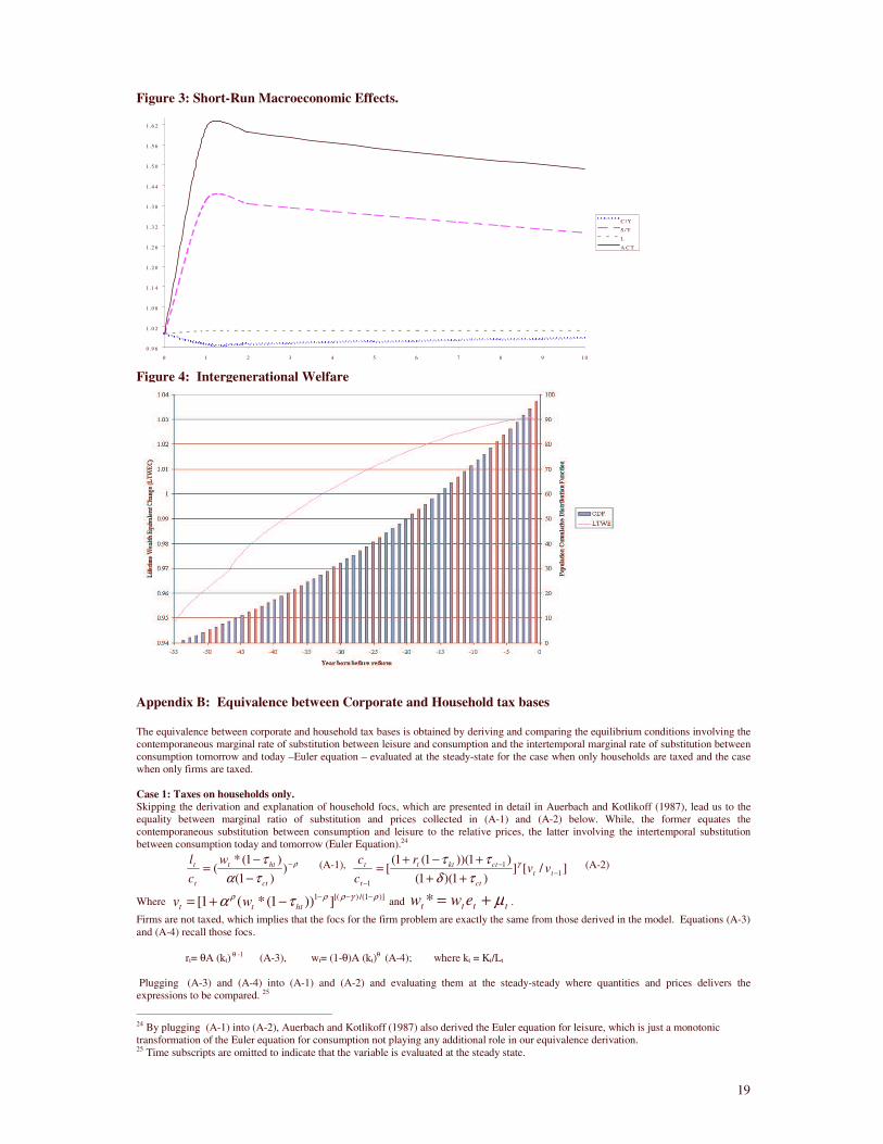
total revenues raised initial steady-state. For the purpose of our tax experiment this implies that the average consumption tax rate is set endogenously through the transition path in order to raise the necessary amount of revenues compatible with the balanced budget. This tax reform experiment will be evaluated by two different criterions. The first is how the economy responds in terms of macroeconomic performance. Final steady states and transition path values of aggregate allocations such as saving rates, national income and physical capital along with wages and interest rates will be analyzed. This first criterion deals with the question of which experiments present the best growth performance in between steady states. The second criterion looks at how different generations will have their lifetime utility levels affected by the proposed fiscal experiment. The question of interest here is who are the winners and who are the losers after the reform. This is a legitimate question to be asked in any democratic economy where the policymaker is interested in evaluating public opinion’s reaction to the reform as a way to infer the political gains she or her elected superior would obtain from the reform. An answer to this question may also provide important information to assess whether a fiscally responsible reform is also political feasible. Subsection A and B deal separately with the macroeconomic performance and welfare effects of the proposed tax reform. Some sensitivity analysis is conducted in subsection C in order to check the robustness of the reform to changes in preference parameters. A. Macroeconomic Effects. The reform resulted in an increase the savings rate followed by an increase in the stock of physical capital, an increase in the supply of labor and an increase in output throughout the transition between steady-states. Table 6 summarizes the impact of the tax reform on GDP components, fiscal variables, production factors quantities and prices along the transition between steady-states. It presents the evolution in each of this variable in the 150 periods that separates the initial and the final steady state. The evolution in each variable is measured relative to the value observed in the initial steady state. Most of the impact of the reform was concentrated in the first years of the transition as illustrated in Figure 3 A partial switch to a consumption tax system generates significantly more long run capital formation than a combined income and consumption tax system. The savings rate (S/Y) presents a substantial increase of 40% in the first year. It decreases afterwards but still presents a long run increase of 8%. The consumption rate (C/Y) decreases in the first year by 3%, slowly increasing in the first ten years to finally reach a long-run level 2% larger than in the initial steady-state. The average consumption tax rate (ACT) jumped by 60% in the first years, slowly decreasing in the remaining years to a value still 30% higher in comparison to the initial steady state. After a slight decrease of 1% in the first year, the capital-labor ratio (K/L) steadily increase in the remaining years to a level more than 15% higher after 50 years. The growth in the capital-labor ratio was followed by a continuos increase in wages and a decrease in interest rates. In order to understand these results we need to look at the income and substitution effects derived from this proposed reform. The revenue-neutrality of the tax reform basically implies that the total amount of resources the tax system extracts from the private sector after the reform is identical to the level extracted before the reform. Therefore, the income effects arising from the proposed reform are the result of distribution between groups and not of an overall change in private sector resources. The reform, however, by altering the pattern of incidence of the tax system, changes the amount of resources extracted from different groups in the private sector. Recall from the previous section that heterogeneity in the private sector is limited in the model by age.

13

Older generations, being closer to the end of their lifetime, present in this model a higher marginal propensity to consume and therefore, cannot escape from the new consumption tax by delaying consumption to future years.20 Based on this argument, the older is the generation, the closer is the lump-sum nature of the new consumption tax and the more negative will be its income effect. Younger generations, on the other hand, present a lower marginal propensity to consume (a higher marginal propensity to save). Although, younger generations still have to pay the same amount in taxes over their lifetime they had to pay before the reform, the bulk of the payment can be postponed to the end of her lifetime when marginal propensity to consume increases. Under positive interest rates, the result is a reduction in the present value of lifetime tax payments and an increase in their lifetime income. But the income effect described above is not the only force driving the increase in aggregate income, savings and capital promoted by the reform. The positive income effect to the young and future cohorts is compounded by a positive substitution effect of higher after tax interest and wage rates resulting from the reduction of labor and capital income taxes and above all by a declining consumption tax rate. As a result of that the reform induced those individuals to procrastinate their consumption even further in order to take advantage of future lower after tax prices. The path for aggregate consumption is less clear. In the initial periods of the transition, where a larger percentage of the consumption should come from older generations born before the reform and whose lifetime income decrease after it, aggregate consumption should decrease. As times goes by, generations who were young at the time of the reform start to increase their participation in the aggregate consumption. Given the positive income effects they will consume more than they would have consumed had the tax reform not been implemented. The result would be an increasing consumption. The average consumption tax rate should increase in order to balance the budget as it was explained before. The increase should be particularly accentuated in the first periods of the transition when aggregate consumption decreases. As aggregate consumption starts to increase again, the required tax rate should start to decrease. Under the fiscal adjustment condition tax revenues and government expenditures are set constant along the transition. The average tax burden (tax revenues over GDP) and the primary surplus (tax revenues minus government expenditures) will start decreasing as soon as GDP starts increasing. The path of interest and wage rates will depend on the path of capital-labor ratio emerging after the reform. If the growth in capital is larger than the increase in labor supply, the ratio should increase. Given the decreasing return nature of the technology, the increase in the capital-labor ratio would imply a decrease in interest rate and an increase in wages. The results presented above seem to indicate that the expected long-run positive growth effects of switching to a consumption-based system commonly obtained in the literature are replicated for the Brazilian economy. The imposition of the additional fiscal stress condition does not compromise the long-run results. Neither it imposes short-run costs in terms of a substantial decrease in individual savings, consumption, employment or income for the first years of the transition. B. Welfare Effects. Replacing taxes on corporate revenues by an additional tax on consumption seems to be implementable even under fiscal stress. It remains to be analyzed whether the same reform would be able to be implemented in a society where public opinion is valued by the policymaker.

20 Recall that no bequests are left in this model.

14

Public opinion reactions to the tax reform could be inferred by the number of individuals expecting a lifetime welfare improvement after the reform. Lifetime welfare expected changes (LTWEC) from a fiscal reform are measured as the fraction of the remaining full lifetime labor endowment required under the original tax regime to produce each cohort’s realized level of utility under alternative tax regimes. It is basically an equivalent variation measure of lifetime changes in welfare. A number higher than one means that the cohort in case will need more than the total amount of her full lifetime endowment to produce the level of utility after the reform. This implies that the respective individual would expect to experience a welfare gain if the proposed tax reform is implemented in an once and for all basis, thus being in favour of the reform. From the previous discussion of the macroeconomic effects, it should be clear that the tax reform imposes a redistribution of lifetime wealth from older to younger cohorts living at the time the reform is proposed. The exact number of older (younger) generations experiencing welfare losses (gains) with the reform, however, can only be determined after the tax reform is simulated. This information is summarized in Figure 4. The horizontal axis orders individuals according to the number of years born before the reform. It ranges from –54, (individuals born 54 years before the reform and with one more year of life left after it) to 0 (individuals born at the year the reform is proposed). The left hands side vertical axis measures changes in lifetime wealth experienced by each individual. Points combining individual age and her respective change in welfare are linked by the line in the model. The cumulative distribution function of the population represented by bars in the same figure is measured on the right hand side vertical axis.21 It is clear from this figure that generations born at least 31 years before the reform will present a decrease in their remaining full lifetime income after the reform (LTWEC is smaller than 1), a group that corresponds to little more than 30% of the living population. The remaining 70% of the population are composed of individuals from generations born at most 31 years before the reform, who, on the other hand, will experience an increase in their full lifetime income. Therefore, based on the LTWEC measure the proposed reform would receive the approval of 70% of the population. Whether the high popularity of the reform will imply its implementation in a representative democracy is a much more complicated issue. Factors such as the correspondence between demographical and political representation in the legislature, the size of majority required to approve the reform and the strategic voting behavior of congressional representatives, just to name a few will have to be considered. Consider a simple political mechanism to aggregate preferences where the proposed tax reform is voted by all living individuals under the expectation that the reform once implemented will last for the remaining of their life.22 Political and demographical representation are identical in this case. A referendum would be the closest real life political process to the one proposed above. Under this political mechanism, there is a one to one correspondence between the popularity of the reform and its implementation likelihood. The larger is the number of individuals experiencing welfare improvements for their remaining lifetime, the larger the approval rate for the reform and the larger the number of votes this reform would receive. Under this simple political mechanism our proposed tax reform would be implemented under majority rule (50% +1 votes) and even under supermajority requirements of up to 3/5 of the votes.23

21 Recall that population growth is approximately 2% meaning that each cohort has 2% more individuals than the previous one. 22 This assumption is essential to make the individual voting decision compatible with the LTWEC. 23 The intergenerational distributive impacts did not show to be sensitive to the selection of preference parameters either. This point is also illustrated in Table 7 whose last column presents the youngest generation to be hurt by the tax reform. This

15

VI- Conclusions This paper focused on a specific reform that could potentially overcome the fiscal stress restrictions central to the implementation of more fundamental reforms in the Brazilian tax system. The reform consisted basically of replacing the indirect taxes on corporate revenues, which are shown to be equivalent to a symmetric tax on labor and capital income, by a new federal VAT whose revenues are not shared either with states or with municipalities. Replacing federal taxes on corporate revenues by this new federal contribution under a balanced budget brought a positive long-run income growth. This improved macroeconomic performance did not involve any substantial short-run decrease in income, the supply of labor, capital accumulation, increase in interest rates, decrease in wages, macroeconomic indicators usually considered by the private sector when evaluating the implementability of any tax reform. This proposed reform has also shown to redistribute income from an old and rich minority to a young and poor majority, a result that would be very likely to be implemented in a referendum where living generations would have equal participation. This should also be a popular result that will certainly be embraced by members of the political class in any democratic regime. The tax reform proposal simulated in this paper should be seen not as a substitute but as a complement to the more comprehensive tax reform proposals whose main features have already been carefully appreciated by the Brazilian National Congress. As it has been shown, it falls short on eliminating all sources of distortion aimed at by other proposals and, because of that, should be considered just as a first step towards a better tax system. Nonetheless, the macroeconomic and welfare effects revealed in simulations of this proposed reform are positive enough to encourage its immediate appreciation. References. Afonso, Jose Roberto and Araujo, Erika. “ Carga Tributaria : Evolucao Historica (ou Involucao?)”, Informe-se/ Secretaria de Assunto Fiscais, BNDES, n.7, Fev 2000. Araujo, C. Hamilton and Ferreira, Pedro Cavalcanti. “ Reforma Tributaria, Efeitos Alocativos e Impactos de Bem-Estar.”, Revista Brasileira de Economia, vol 53, nº 2, abril/junho, 1999 Auerbach, Alan and Kotlikoff, Lawrence. Dynamic Fiscal Policy, Cambridge: Cambridge University Press, 1987. , Altig D., Smetters, K and Walliser, J. “Simulating Fundamental Tax Reform in the United States.”American Economic Review, 91(3), June 2001 Barreto, Flavio A. and Schymura, L.G. “ Privatizacao da Seguridade Social no Brasil :Um Enfoque em Equilibrio Geral Computavel.” in Anais do XIX Encontro Brasileiro de Econometria,1997 v.1, pp 43-63. Cassou, S.P. and Lansing, Kevin. “Growth Effects of a Flat Tax.”, Fed-Cleveland Working Paper no. 9615, December 1996 Cifuentes, Rodrigo. “ Reforma de los Sistemas Provisionales: Aspectos Macroeconomicos.”, Cuadernos de Economia, 32 (96), August 1995 Cooley, T. F. and Prescott, E. “Economic Growth and Business Cycles in Frontiers of Business Cycle Research, Princeton University Press, Princeton, 1995. Dain, S. “Visões Equivocadas de uma Reforma Prematura.” in Federalismo no Brasil, Affonso, R, and Silva, Pedro eds, Sao Paulo: Editora Unesp-Fundap, 1995 Ferreira, Sergio Gomes. “Studying Macroeconomic Effects of Social Security Privatization in Brazil”, Mimeo, University of Wisconsin-Madison, 2001. Ghez, G. and Becker, Gary S. “ The Allocation of Time and Goods over the Life Cycle.”, New York: Columbia University Press, 1975.

value ranged from –35 to –27, meaning that the youngest generations losing with the implementation of the reform were born between 35 and 27 years before the reform. Under both cutoff points the demographic representation of the generations experiencing welfare gains from the reform was still superior to those experiencing welfare losses. Moreover, the likelihood of the tax reform being implemented in a direct democracy did not substantially change as the size of the winning coalition in all different scenarios was still above 60% of the living population.

16

Giovanni, J. “Saving and Real Interest Rate in LDC.”, Journal of Development Economics, 18, 197-217, 1985. Hofman, Andre A. “ Capital Acumulation in Latin America: A Six Country Comparison for 1950-1989.”,, Review of Income and Wealth, Series 38, n. 38, 1992. Jones, Larry; Manuelli, Rodolfo; and Rossi, Peter. “ Optimal Taxation in Models of Endogenous Growth.”, Journal of Political Economy, June 1993, 101, 485-517. King, Robert G. and Rebelo, Sergio. “Public Policy and Economic Growth: Developing Neoclassical Implications.”, Journal of Political Economy, October 1990, no. 5, pt.2, S126-S150. Krussel, Per; Quadrini, Vincenzo; and Rios-Rull, J.V. “ Are Consumption Taxes really better than Income taxes?”, Journal of Monetary Economics, 1996, 37, 475-503. Lemgruber, Andrea. “ O Processo de Reforma Tributaria no Brasil: Mitos e Verdades”, V Prêmio de Monografia da Secretaria do Tesouro Nacional, Brasilia: Secretaria do Tesouro Nacional, 2000 . Lucas, Robert E., Jr. “ Supply-Side Economics: An Analytical Review”, Oxford Econ. Papers, April 1990, 42, 293-316. MaCurdy, Thomas E., “ An Empirical Model of Labor Supply in a Life Cycle Setting.”, Journal of Political Economy, 89(6), December 1981. Schmidt-Hebbel, Klaus. “Colombia’s Pension Reform: Fiscal and Macroeconomics Effects”. Working Paper. The World Bank. Washington, DC. 1995. Stokey, Nancy and Rebelo, Sergio. “ Growth Effects of Flat-Rate Taxes”, Journal of Political Economy, 1995, 103(3), 519-550. Werneck, Rogerio. “Tax Reform in Brazil: Small Achievments and Great Challanges.”, Texto para Discussao n. 436, Department of Economics, Catholic University of Rio de Janeiro, December 2000 Appendix A : Tables and Figures Figure 1: Evolution of the Tax Burden

Source : Afonso and Araujo (2000) Table 1: Tax Reform Proposals: Comparison of Main Features Proposal Taxes to be Eliminated Taxes to be Created Executive Proposal 08/1995 (PEC 175) IPI,ICMS Dual VAT Executive Proposal 09/1997 COFINS,PIS/PASEP, IPI,

ICMS,ISS Federal VAT, Federal excise tax on goods,State retail sales tax on goods (IVV-S), Municipal retail sales tax on services (IVV-M)

Executive Proposal 10/1999 COFINS,PIS/PASEP,IPI, ICMS, ISS

Federal VAT,Federal excise tax on goods,State excise tax on goods and services,Municipal retail sales tax on services (IVV)

Special Committee Proposal 12/1999 COFINS,PIS/PASEP,CPMF IPI,ICMS, ISS

Dual VAT (coexisting federal and state VATs;same base; different tax rates) Municipal retail sales tax on services (IVV)

Rapparteur’s Proposal 03/2000 COFINS,PIS/PASEP,CPMFSal.Ed, IPI,ICMS,ISS

Dual VAT Federal “non-cumulative” excise tax (to replace COFINS,PIS/PASEP,CPMF,Sal Ed, ISS)

Executive Proposal 08/2000 IPI, ICMS, ISS Federal tax on goods and services,Nationally uniformed state VAT Municipal retail sales tax (IVV)

Source : Lemgruber (2000) and Werneck (2000)

17

Figure 2: Evolution of indirect tax system.

Note : Cumulative taxes = Finsocial/Cofins, PIS/PASEP, IPMF/CPMF, IOF, ISS, Selective taxes. Source : Afonso and Araujo (2000) Table 2 : Distribution of the Burden by Statutory Base Base % GDP % Total1)Indirect Taxes 22.65% 79.12%a) Value-added/Excise 9.68% 33.83%ICMS (State) 7.11% 24.83%IPI (Federal) 1.95% 6.82%II (Federal) 0.62% 2.18%b) Cumulative 4.97% 17.38%b.1) Corporate Revenues 3.67% 12.84%COFINS (Federal) 2.22% 7.77%PIS/PASEP (Federal) 0.90% 3.13%ISS (Local) 0.55% 1.94%b.2) Financial Transactions 1.30% 4.54%IOF (Federal) 0.47% 1.66%CPMF (Federal) 0.83% 2.88%c) Corporate Payroll (Federal) 7.99% 27.91%Social Security Retirement 4.81% 16.80%SED + FGTS +Others 3.18% 11.11%2) Direct Taxes 5.98% 20.88%a) Personal Income 1.96% 6.83%IRPF (Federal) 1.96% 6.83%b) Corporate Income 2.89% 10.11%IRPJ (Federal) 2.06% 7.21%CSLL (Federal) 0.83% 2.90%c) Property 1.13% 3.95%IPTU (Local) 0.41% 1.44%IPVA (Local) 0.38% 1.32%Others (ITR +ITBI)(Federal) 0.34% 1.18%3) Total w/out SS retirement 23.82% 83.20%4) Total Tax Burden 28.63% 100.00% Source : IBGE- Department of National Accounts, BNDES – Secretary of Fiscal Affairs Table 3: Average Tax Rate Computation

18

Notes: Average tax rate equivalence hypothesis – 1)Value added is consumption,2)Property tax base is personal income, 3) Financial transactions is corporate revenue, 4) Corporate Profit is a) capital income, b)personal income, 5) Corporate payroll is labor income, 6) Corporate revenues is personal income Table 4: Benchmark Parameter Definitions and Values.

Symbol Definition Value et Earnings Ability Profile et =exp(a +bt +ct2 ) a/b/c -0.231/ 0.0529/- 0.000934

ηηηη Population growth 0.019 ρρρρ Elasticity of substitution b/w consumption and leisure 1.15 γγγγ Intertemporal elasticitity of substitution in consumption 0.40 αααα Weight preference for leisure 0.25 δδδδ Intertemporal discount rate 0.021 θθθθ Capital share in income 0.50 Taxes in initial steady-state : ττττi i=c,y,k,l ττττc Consumption tax rate 0.157

ττττy Ovreall income tax rate 0.105 ττττk Capital income tax rate 0.092 ττττl Labor income tax rate 0.076 Table 5: Initial Steady-State

Note : Y=GDP, C/Y = consumption rate, S/Y- Depr/Y = net savings rate, K/Y= capital-output ratio, T/Y= Total tax burden (SS not included), SStax = Social Security Tax rate, G/Y=public expenditures rate, rD/Y = public debt service payments, Gss/Y = Social Security benefit rate, D/Y =overall public sector debt rate r= interest rates. Table 6: Replacing Taxes on Corporate Revenues by an additional consumption tax (i) Once and for all at period 1, (ii) Under a balanced budget.

0 1 2 3 4 5 6 7 8 9 10 50 150

GDP 1.00 1.00 1.01 1.01 1.02 1.02 1.02 1.03 1.03 1.03 1.03 1.08 1.09Composition of GDPConsumption (%GDP) 1.00 0.97 0.97 0.97 0.97 0.98 0.98 0.98 0.98 0.99 0.99 1.02 1.02Savings (%GDP) 1.00 1.40 1.38 1.37 1.36 1.35 1.34 1.33 1.32 1.31 1.30 1.10 1.08Fiscal VariablesAv. Consumption Tax 1.00 1.61 1.60 1.58 1.56 1.55 1.54 1.52 1.51 1.50 1.49 1.30 1.28Tax Revenues (% GDP) 1.00 1.00 0.99 0.99 0.98 0.98 0.98 0.97 0.97 0.97 0.96 0.91 0.91Primary Fiscal Surplus (% GDP) 1.00 1.00 0.99 0.98 0.97 0.97 0.97 0.96 0.95 0.95 0.94 0.86 0.85Input Quantities and PricesCapital (%GDP) 1.00 1.00 1.00 1.00 1.01 1.01 1.01 1.02 1.02 1.02 1.02 1.07 1.08Labor Supply 1.00 1.01 1.01 1.01 1.01 1.01 1.01 1.01 1.01 1.01 1.01 1.01 1.01Wages 1.00 1.00 1.00 1.00 1.01 1.01 1.01 1.02 1.02 1.02 1.02 1.07 1.08Interest Rates 1.00 1.00 1.00 1.00 0.99 0.99 0.99 0.98 0.98 0.98 0.98 0.93 0.93 Table 7 : Sensitivity Analysis

LosersGamma Delta Rho Alpha Y C/Y K/Y L ACT Year Born

0.4 0.02 1.15 0.25 9 2 8 1 28 -320.3 0.02 1.15 0.25 9 3 8 1 27 -350.9 0.02 1.15 0.25 9 2 8 1 32 -270.4 0.01 1.15 0.25 9 2 8 1 27 -320.4 0.05 1.15 0.25 9 2 8 1 27 -350.4 0.02 0.8 0.25 8 2 8 0 31 -310.4 0.02 1.5 0.25 9 3 8 1 27 -330.4 0.02 1.15 0.05 9 2 8 0 28 -340.4 0.02 1.15 0.6 9 2 8 1 29 -29

Paramaters % Variation between steady-states

19

Figure 3: Short-Run Macroeconomic Effects.

0 .9 6

1 .0 2

1 .0 8

1 .1 4

1 .2 0

1 .2 6

1 .3 2

1 .3 8

1 .4 4

1 .5 0

1 .5 6

1 .6 2

0 1 2 3 4 5 6 7 8 9 1 0

C /Y

S /Y

L

A C T

Figure 4: Intergenerational Welfare

Appendix B: Equivalence between Corporate and Household tax bases The equivalence between corporate and household tax bases is obtained by deriving and comparing the equilibrium conditions involving the contemporaneous marginal rate of substitution between leisure and consumption and the intertemporal marginal rate of substitution between consumption tomorrow and today –Euler equation – evaluated at the steady-state for the case when only households are taxed and the case when only firms are taxed. Case 1: Taxes on households only. Skipping the derivation and explanation of household focs, which are presented in detail in Auerbach and Kotlikoff (1987), lead us to the equality between marginal ratio of substitution and prices collected in (A-1) and (A-2) below. While, the former equates the contemporaneous substitution between consumption and leisure to the relative prices, the latter involving the intertemporal substitution between consumption today and tomorrow (Euler Equation).24

ρ

τατ −

−−

= ))1(

)1(*(

ct

htt

t

t wcl (A-1), ]/[]

)1)(1()1))(1(1(

[ 11

1−

−

− +++−+

= ttct

ctktt

t

t vvr

cc γ

τδττ (A-2)

Where )]1/()[(1 ]))1(*(1[ ργρρρ τα −−−−+= httt wv and tttt eww µ+=* .

Firms are not taxed, which implies that the focs for the firm problem are exactly the same from those derived in the model. Equations (A-3) and (A-4) recall those focs.

rt= θA (kt) θ -1 (A-3), wt= (1-θ)A (kt)θ (A-4); where kt = Kt/Lt

Plugging (A-3) and (A-4) into (A-1) and (A-2) and evaluating them at the steady-steady where quantities and prices delivers the expressions to be compared. 25

24 By plugging (A-1) into (A-2), Auerbach and Kotlikoff (1987) also derived the Euler equation for leisure, which is just a monotonic transformation of the Euler equation for consumption not playing any additional role in our equivalence derivation. 25 Time subscripts are omitted to indicate that the variable is evaluated at the steady state.

20

ρ

θ

τα

τµθ

−

������

�

�

������

�

�

−

−��

��

�

+−

=)1(

)1()1(

c

hekA

c

l

(A-5) , γθ

δτθ

��

���

�

+−+

=−

)1()1)((1

11

kAk (A-6)

Case 2: Taxes on firms only. Marginal rates of substitution for the case when just firms are taxed are identical to the previous one except that after tax prices are identical to before tax prices. One would need just to rewrite (A-3) and (A-4) by setting all taxes equal to zero.

ρ

α−= )

*( t

t

t wcl (A-7) , ]/[]

)1(1

[ 11

−− +

+= tt

t

t

t vvr

cc γ

δ (A-8)

Where )]1/()[(1 ]*)(1[ ργρρρα −−−+= tt wv

The basic change will be on the firm focs. Recall that the problem of the firm consists basically on the static maximization of profits, after tax profits if they are taxed. Under the latter case the firm optimization problem can be rewritten as follows:

Max Yt - wt Lt - rt Kt - Tt (A-9)

Where Tt is the total amount the firm has to pay in taxes. Tt can assume different forms, depending on the incidence base. In this simple model, we are going to consider three different bases: corporate revenues, payroll and profit. Suppose that firms are taxed at a proportional rate τp. Taxes on corporate revenues. Yt, the total amount of the final good produced by the firm, in equilibrium can also be seen as the firm revenues. A proportional tax on firm revenues is represented by Tt =τpt Yt (A-10) Focs for the firm problem are now obtained by solving (A-9) subject to (A-10). Input factor prices are now:

rt= (1-τpt) θA (kt) θ -1 (A-11), wt= (1-τpt) (1-θ)A (kt)θ (A-12); Substituting (A-11) and (A-12) into (A-7) and (A-8) evaluating at the steady-state generates the steady-state focs.

ρ

θ

τα

τθ−

�����

�

�

�����

�

�

−

��

��

�

−−

=)1(

)1()1(

c

pekA

c

l(A-13) ,

γθ

δτθ

��

�

�

��

�

�

+−+

=−

)1(

)1)((11

1pAk (A-14)

(A-13) and (A-14) are identical to (A-5) and (A-6) iff τp=τk=τh . Taxing corporate revenues is equivalent to imposing a symmetric tax on capital and labor income in the steady state. The implication of that result for the calibration of the Auerbach and Kotlikoff (1987) model is that it suffices to consider an average rate on corporate revenue as an additional tax rate on overall income. With perfect competition in the final and input good markets, the firms are not able to shift the tax forward to consumers. Therefore, the entire tax is borne by the firm owners, which are the individuals holding capital. Taxes on payroll A proportional tax on the firm payroll -Tt = τpt wt Lt - generate the new focs below:

rt= θA (kt) θ -1 (A-15), wt= (1-τpt)-1 (1-θ)A (kt)θ (A-16) ; Substituting (A-15) and (A-16) into (A-7) and (A-8) evaluating at the steady-state generates the steady-state focs:

ρ

θ

α

τθ−

−

�����

�

�

�����

�

�

��

��

�

−−

=ekA

c

lp

1)1)(1( (A-17), γθ

δθ

��

���

�

++=

−

)1()(1

11Ak (A-18)

(A-17) and (A-18) are identical to (A-5) and (A-6) iff τh= τp/1-τp . Taxes on real profits. Let’s start here by distinguishing the firm pure profit - Yt - wt Lt - rt Kt, which is always equal to zero by the long-run perfect competition assumption and the the firm real gross profit, the profit the firm obtains after servicing their payroll obligations. Given the simplifications of this model, the gross profit is the resource the firm is going to distribute to their household owners before the collection of taxes. Revenues from a tax on real gross profits are given by: Tt =τpt (Yt - wt Lt) (A-19) Firm focs are now: rt= (1-τpt) θA (kt) θ -1 (A-20) , wt= (1-θ) A (kt)θ (A-21) Substituting (A-20) and (A-21) into (A-7) and (A-8) evaluating at the steady-state generates the steady-state focs:

ρ

θ

α

θ−

�����

�

�

�����

�

�

��

��

�

−

=ekA

c

l)1( (A-22),

γθ

δτθ

��

�

�

��

�

�

+−+

=−

)1(

)1)((11

1pAk

(A-23)

(A-22) and (A-23) are identical to (A-5) and (A-6) iff τp=τk. Taxes on real profits are identical to taxes on household capital income.