Embed Size (px)
Citation preview
TEXTO PARA DISCUSSÃO N°°°° 172
SOCIAL INEQUALITY IN THE ACCESSTO HEALTHCARE SERVICES IN BRAZIL
Kenya Valeria Micaela de Souza NoronhaMônica Viegas Andrade
Junho de 2002
2
Ficha catalográfica
33:614(81)N852s2002
Noronha, Kenya V. M. S.Social inequality in the access to healthcare services in Brazil /
Kenya V. M. S. Noronha ; Mônica Viegas Andrade. - BeloHorizonte: UFMG/Cedeplar, 2002.41p. (Texto para discussão ; 172)
1. Serviços de saúde – Brasil. 2. Economia da saúde – Brasil.3. Brasil – Condições sociais. 4. Brasil – Condições econômicas.I. Andrade, Mônica Viegas. II. Universidade Federal de MinasGerais. Centro de Desenvolvimento e Planejamento Regional. III.Título. IV. Série.
3
UNIVERSIDADE FEDERAL DE MINAS GERAISFACULDADE DE CIÊNCIAS ECONÔMICAS
CENTRO DE DESENVOLVIMENTO E PLANEJAMENTO REGIONAL
SOCIAL INEQUALITY IN THE ACCESS TOHEALTHCARE SERVICES IN BRAZIL
Kenya Valeria Micaela de Souza NoronhaAluna de Economia
Mônica Viegas AndradeProfessora do Cedeplar/UFMG
CEDEPLAR/FACE/UFMGBELO HORIZONTE
2002

4

5
SUMÁRIO
1. INTRODUCTION ............................................................................................................................ 7
2. REVIEW OF THE LITERATURE .................................................................................................... 82.1. Review of the International Empirical Literature ............................................................................ 82.2. A Review of the Brazilian Empirical Literature .............................................................................. 9
3. DATABASE AND DESCRIPTION OF VARIABLES ................................................................ 103.1. Descriptive Analysis of the Behavior of Major Variables ............................................................. 13
4. METHODOLOGY ........................................................................................................................... 164.1. The Negative Binomial Hurdle Model .......................................................................................... 164.2. Specification Tests ......................................................................................................................... 204.3. Interpretation of Coefficients ......................................................................................................... 21
5. MAJOR RESULTS ....................................................................................................................... 225.1. Is there social inequality in the access to healthcare services in Brazil? ....................................... 23 5.1.1. Ambulatory services ............................................................................................................. 23 5.1.2. Inpatient Care ...................................................................................................................... 265.2. Access to healthcare services, according to the supply characteristics ......................................... 28 5.2.1. Ambulatory services ............................................................................................................. 28 5.2.2. Hospitalization services ....................................................................................................... 285.3. Access to healthcare services, according to the needs .................................................................. 29
6. FINAL REMARKS .......................................................................................................................... 30
7. REFERENCES ................................................................................................................................. 31
ECONOMETRIC ANNEX ................................................................................................................... 33

6
7
1. INTRODUCTION
The major health policy goal in most countries has been the promotion of an equitablehealthcare distribution. However, empirical works point out to a general healthcare inequality whichfavors more privileged social groups. Brazilian studies also indicate social health inequality favoringhigh-income groups1. This result can be a consequence of differences in the amount of medicalassistance between socioeconomic groups. Empirical evidence shows that there is inequality in theaccess to healthcare in some countries which is favorable to the wealthy2. Such an outcome was evenobserved in developed countries where economic disparities are not so outstanding and in countries inwhich healthcare services are free of charge.
The social inequality in health and the way healthcare services supply is organized in Brazilsuggest the presence of social inequality in the access to such care. The Brazilian healthcare market ischaracterized as a mixed system both in funding and provision, implying two different types of access.Firstly, a common public healthcare system is offered – the Sistema Único de Saúde (SUS). In thiscase the supply of health care services is universal, comprehensive, and free. Secondly, there are thehealth care services funded and provided by the private sector. In this case the access is guaranteedagainst out-of pocket payment to providers or by adhesion to a health insurance plan.
This aim of this paper is to test the hypothesis of horizontal equity in the access to healthcareservices in Brazil, considering outpatient and inpatient care separately. This paper intends to verifywhether individuals having equal needs are granted the same healthcare level, independently of theirsocioeconomic characteristics. The estimation method is based on the hurdle negative binomial model(hurdle negbin) which estimates the use of healthcare services in two stages. The database used isPNAD/98 – Pesquisa Nacional de Amostra Domiciliar (the Brazilian National Household SampleSurvey), which presents a special survey on health issues. For every type of health care we consideredtwo different samples: the first one including all age groups and the second one including only theoccupied population at active age (individual between 15 and 65 years old). The latter exercise iscrucial as it allows that the individuals’ occupational characteristics be taken into account.
The major contribution of this paper is to estimate social inequality in the access to theBrazilian healthcare services by using the hurdle model. The findings show that inequality in theaccess to healthcare services is differentiated, according to the kind of healthcare focused. Whenconsidering ambulatory services, we found in the two samples that the greater the family per capitaincome, the greater the probability of an individual to visit a doctor. This is also observed even whenthe morbidity and occupational characteristics and the existence of a healthcare plan are controlled.The expected number of medical visits is responsive to income only when the sample is restricted tooccupied individuals. The greater the income, the greater the number of doctor visits. A possibleexplanation for such an outcome is that, when the total population is considered, the most vulnerablepopulation groups in terms of health status - children and the elderly, who can not postpone medicalassistance – are included.
1 For international literature, see Pereira, 1995 e Doorslaer et al, 1997. For the Brazilian case, see Noronha e Andrade, 2001,
Campino et al, 1999, and Travassos et al, 2000.2 Pereira, 1995, Doorslaer e Wagstaff, 1992 e Waters, 2000.
8
Related to inpatient care we observed that the probability of individuals to be hospitalized andthe time span are greater for the poorer, if the whole sample is considered, characterizing inequality inthe access in favor of the poor. Such a result, however, should be interpreted with caution, as healthmeasures used may not be capturing the differences in the degree of morbidity between the poor andthe wealthy. Poorer individuals may present a more precarious health status when they look forhealthcare, needing a more intensive treatment.
This paper is divided into five sections beyond this one. In the next section, both a reviewconcerning the usually employed methods in the international literature and the empirical evidence inBrazil will be made. The third section presents a brief description of the database and variables used.The fourth section discusses the methodology. The major outcomes are presented in the fifth section.The last section presents the final remarks.
2. REVIEW OF THE LITERATURE
2.1. Review of the International Empirical Literature
Social inequality in the access to healthcare services has been widely analyzed in severalempirical works in the international economic literature. The criterion usually adopted is based onhorizontal equity principle (individuals with equal healthcare needs should be treated in the sameway). Based on such principle, health care services should be distributed in accordance with thehealthcare needs of each individual, independently of his/her socioeconomic characteristics. Basically,there are two ways of verifying if the healthcare system follows the equity principle.
The first consists in measuring inequality in the access of healthcare services. Initially,empirical works reported in the international literature were based on the construction of concentrationcurves relating the access to healthcare services to morbidity incidence in each socioeconomic group.Le Grand (1978) pioneered the use of such a methodology which was further developed by Doorslaerand Wagstaff (1992). Based on such a methodology, Campino et al (1999) measured the socialinequality in the access to healthcare services in Brazil. The authors measured the access to health careservices through utilization which allowed them to build two concentration curves: the firstunstandardized and the second standardized by age, sex, and morbidity. The results encounteredsuggest the existence of social inequality in the preventive and curative health care services favoringhigher income groups.
A second way of evaluating inequality in the access to healthcare services consists inestimating a regression model whose dependent variable encompasses a utilization measure. The firstwork to employ such a method was developed by Cameron et al (1988). The authors estimated anequation of health services utilization for Australia, based on a binomial negative model to verify thefrequency in which individuals used healthcare services. The major contribution of this paper was toconsider the health insurance choice as an endogenous variable.
Some authors have proposed to estimate the model of healthcare services utilization in twostages. In the first stage, the probability of people receiving or not healthcare services would be
9
estimated; and in the second stage, the amount of health care services would be estimated consideringonly individuals in the sample with positive utilization. In the first estimation stage, a binaryprobability model (Logit or Probit) is used for estimating whether the individual searched or not forany healthcare service. The estimation in the second stage may be accomplished in several ways. Oneof these consists in estimating the regression for a frequency decision by the Ordinary Least Squaremethod (OLS)3. The weak point of such a method is that data on utilization of healthcare services arecensored. When estimating by OLS, this particularity of the sample is ignored4. A second way consistsin estimating a hurdle model in which the second stage is estimated adopting a truncated at zeronegative binomial model5. Gerdtham (1997) and Pohlmeier and Ulrich (1994) use this methodologyfor testing the horizontal equity in the access to healthcare services in Sweden and Germany,respectively considering the adult population. In the two studies, contact decision and the frequencydecision are determined by distinct stochastic procedures which suggest that estimation through thehurdle model is more adequate.
Both works estimate separate models for the different health care specialties. Gerdtham (1997)distinguishes the ambulatory services from inpatient care. According to the author, such demands cannot be interpreted in the same way, due to the fact that the probability of hospitalization dependsmainly on a physician’s decision, whereas the probability of a doctor visit depends on the decision ofthe individual him/herself. Pohlmeier and Ulrich (1994) distinguish the generalist doctor from thespecialist doctor. Such a distinction is relevant, due to the characteristics of healthcare services inGermany. Access to specialist physicians is mainly accomplished through an referral from a generalistphysician which thus defines differentiated behaviors in relation to healthcare services demandbetween the two medical specialties.
2.2. A Review of the Brazilian Empirical Literature
As far as the Brazilian case is concerned, there are some papers which attempt to measuresocial inequality in the access to healthcare services. Almeida et al (2000), based on the PNSN6 for theyear of 1989, estimated a healthcare service utilization rate for each income quintile. These rates werestandardized by sex and age and obtained separately for sick and healthy individuals. The healthcareservice utilization is strongly unequal among the socioeconomic strata, favoring the higher-incomelevels. Approximately 45% of the individuals belonging to the first quintile with activities restraineddue to illness use healthcare services. This percentage increases to 69.22% when higher-incomegroups are considered. For the sample of healthy individuals, the fifth quintile shows a utilization rate50% higher than that for the lowest-income stratum. 3 Alberts et al, 1997, and Doorslaer and Wagstaff, 1992.4 Some authors also point out to the problem of sample selection bias. In this case, the model used is based on the
methodology developed by Heckman (1979), consisting in estimating, in the first stage, an equation for the search of healthservices through the Probit model through which a correction factor of the sample selection bias is obtained. Such a factoris included in the regression model to estimate, through the LOS, the frequency of doctor visits. See, e.g., Newbold, Eylesand Birch (1995).
5 The hurdle model was initially proposed by Mulahy (1986), and is used by some authors in the analysis of the access tohealth services.
6 A national survey on health and nutrition.
10
Travassos et al (2000) estimated odd ratios for three income groups by using a PPV for theyears of 1996/19977. The authors showed that there is social inequality in the distribution of healthcarein the country, which is favorable to privileged social classes. The chances of an individual of the firsttercile to use healthcare services is 37% smaller in the Brazilian Northeast and 35% smaller in theSoutheast, as compared to individuals in the third tercile. Utilization chances are also greater amongindividuals covered by health insurance plans vis à vis those not covered (66% greater in the Northeastand 73% in the Southeast).
Viacava et al (2001), based on data from the PNAD/98 (the National Household SampleSurvey), tested the existence of social inequality in health services utilization by gender. They alsoestimated odds ratios. The authors observed that individuals with higher education degree, employers,formal sector employees, and whites have greater chances to search for healthcare services bothpreventive and curative services. This indicates social inequality in the consumption of such services,favoring more privileged social groups.
Empirical studies in Brazil suggest the presence of social inequality in the access to healthcareservices. The aim of this paper is to go further in this discussion using a methodology that allows us toevaluate if the existing inequality in this market is related to the contact decision or to the frequencydecision - the amount of treatment to be received by the patient.
3. DATABASE AND DESCRIPTION OF VARIABLES
The database used was the PNAD/98, accomplished by the Instituto Brasileiro de Geografia eEstatística – IBGE – (the Brazilian census bureau), containing information on individualcharacteristics, such as education level, individual and family income, age, among others. In 1998, thesupplement of PNAD focused on health issues8. 344,975 people were surveyed all through the nationalterritory, except for the Northern region’s rural area. For this reason, all the federative units of thisregion were excluded from the analysis which reduced the number of observations to 318,9099.
The dependent variables encompass a measure of physician care and hospitalizations10. Thesevariables were obtained from questions in PNAD/98 which allowed us to know whether theindividuals had visited the doctor and on what frequency as well as whether they had been hospitalizedand for how long in the 12 months previous to the survey11.
The independent variables may be classified into three groups. The first comprisessocioeconomic and demographic variables. A set of dummies for per capita family income, head of 7 A survey on standard of living.8 The information contained in the supplement were mostly given by only one person living in the household. 36.08% out of
the respondents in this part corresponded to the person him/herself.9 The sample size varied in accordance with the estimated model due to those missing in the dependent and independent
variables used in each model.10 There are several ways to measure the access to healthcare services. A measure of healthcare services utilization is usually
used. Another method, i.e., through expenditure, is generally used.11 Concerning medical appointments, the PNAD/98 also includes another question using a period of 2 weeks as reference.
This question was not used, because the demand for services was declared by a very small percentage of individuals andthis made it impossible a more detailed analysis.
11
family education, race, gender, and family composition is considered. Furthermore, we included adiscrete variable referring to the number of family members as well as two variables related to age - alinear and a quadratic term. In the model estimated for the occupied population at working age,variables related to individual occupation characteristics, such as occupied position, number ofworkhours, and branches of activity, could be taken into account.
The individuals were grouped according to their income decil12. To account for education, thesample was classified into nine groups according to the schooling of household head13. This variable ismore appropriate than that of the own individual’s education as it allows to include people at schoolage in the sample. Differences in healthcare services utilization may also occur among ethnic groups,due mainly to their relation to the individuals’ socioeconomic position. PNAD/98 included whites,blacks, Asians, mestizos, and Indians in the sample. Only two categories will be considered in thispaper, however: whites and nonwhites.
The family size effect is ambiguous. On the one hand, family size may positively affect thedecision to use healthcare services due to the existence of economies of scale as healthcare cost isnonlinear in the number of family members. For example, when she takes a child to see the doctor, amother may decide to take the other children too, as the opportunity cost of taking the other children isnull for her. On the other hand, it is possible for the parents of a larger family to acquire someknowledge relating healthcare as they have more children (learning by doing) and thus becoming lessdependent on healthcare services when a child becomes ill. In this case, the effect of this variable isnegative. Furthermore, the composition of family expenses may vary according to its size thuschanging the participation of health expenses in the total family budget.
The effect of family size largely depends on its composition, as health expenses and usage ofsuch services are closely related to the age of their members. In this paper, the variable familycomposition was constructed by IBGE. PNAD/98 ranks the individuals into ten groups according tothe kind of family which they belong to14. Due to the small number of observations, individualsbelonging to families comprised by the couple or the mother, whose children’s age had not beendeclared, were aggregated in the group referring to “other kind of family”.
The proportion of individuals using medical services and hospitalizations and the frequencywith which they are used is very differentiated among age groups. These services are expected to bemore used by the extreme age groups, meaning that the children and the elderly need more such carethan the other age groups. A continual age variable containing a linear term and a quadratic term and abinary variable for men were used in order to control such an effect.
12 Individuals whose family income is equal to zero were included in the sample. Such individuals represented 3% of the total
sample (9,099 observations).13 Illiterate and those with less than one year of education, incomplete elementary school, complete elementary school,
incomplete junior high school, complete junior high school, incomplete senior high school, complete senior high school,incomplete higher learning, complete higher learning.
14 Couple with no children, couple with all their children below 14, couple with all their children over 14, couple with theirchildren below 14 and over this age, couple with children of undeclared age, mother with all her children below 14,mother with all her children over 14, mother with children over and below 14, mother with children of undeclared age andother kind of family.
12
The dummy variables related to the occupational characteristics were included in the estimatedmodel for the occupied population at working age15. Such variables allow to measure the opportunitycost for searching for any healthcare service. The time devoted to work implies less available time tosee a doctor. Furthermore, depending on the way individuals enter the labor market, their opportunitycost is greater. People working in the informal labor market are generally paid per worked hour andare not protected by labor legislation. Thus, leaving work activities may result in income loss. Thegreater the loss, the greater the opportunity cost in demanding medical assistance. Two worked-hourgroups were considered: those working between 1 to 39 hours per week and those working 40 hours ormore.
In PNAD/98, the individuals were ranked into 12 positions in the occupation. Based on thesecategories, we constructed seven groups: registered employees in the formal sector; the military andpublic servants; unregistered employees (informal sector employees); house servants, independently ofbeing registered or not; self-employed workers; employers; own-consumption production workers;own-use construction (building) workers; and unpaid family workers. Concerning the branches ofactivity, PNAD/98 specifies eleven categories16. This variable allows the particularities of the labor tobe considered. Some activity branches are associated to a greater health hazard, implying a greaterdemand for medical and hospital assistance.
The second group of variables refers to supply characteristics. Different levels of access tohealthcare services may be related to differences in the supply of such services among the localities.As such information is not provided by PNAD/98, dummies were included for the federative units andfor localization of residences (urban/rural), considering that the supply of healthcare services varygreatly among the states and is precarious in rural areas.
In the model estimated for the ambulatory services, a dummy variable was included for theexistence of health insurance coverage in the two estimation stages. The healthcare plan establishes abetter condition of access and the utilization of such services is greater. In the case of hospitalization,this variable was included only in the first stage of the model. In the second stage, it was possible toverify whether the individual was hospitalized through the SUS or not. A difficulty in such variablewas that 3.48% of the hospitalized individuals were not able to inform whether the service wascovered by this system. As the services provided by the SUS should be free of charge, the individualswho did not pay any value for hospitalization were considered to be included in the SUS. In the sameway, if the individuals paid any value for such hospitalization, they were considered as not included inthe SUS system17.
15 All variables related to occupational characteristics refer to the individual’s situation in the previous two weeks of
reference.16 Agricultural activities, manufacturing, civil construction, other industrial activities, merchandize trading, service rendering,
aid services in economic activities, transport and social communications, public administration, and other activities.17 We concluded that 94.22% of the individuals who were not able to inform whether they were included in the SUS system
did not pay any value for the hospitalization. The criterion adopted in this paper to classify such individuals as covered ornot by the SUS does not entirely solve the problem, since the individuals who paid any value for the hospitalization(23.19%) were covered by the SUS.
13
The third group refers to the variables of the individuals’ needs. Four indicators related to theindividuals’ health status were used. The first refers to some possible problem of physical mobility18.Individuals over 14 years of age were asked whether they had any difficulty in accomplishing theirdaily tasks19. The question allows four answer categories: “unable”, “have great difficulty”, “havelittle difficulty”, “have no difficulty”. The second indicator used was the number of chronic diseases.PNAD/98 formulated questions on the existence of 12 kinds of chronic diseases20. The figures of sucha variable ranged from 0 to 11, indicating the total number of chronic diseases declared by theindividual.. The third variable refers to a measure of self-assessed health status. PNAD/98 takes intoaccount five different answer categories: very good, good, fair, poor, or very poor. The fourthindicator of need is a dichotomic variable informing whether the individual had suffered any difficultyin his/her customary activities, due to any health problem in the weeks previous to the survey. Allhealth variables, except for the number of chronic diseases, were modeled in order to include dummyvariables.
As far as hospitalization is concerned, it was possible to include – in the second stage of themodel - a variable indicating the major healthcare service received when the patient was hospitalized.The following categories were specified: general clinical treatment, delivery, cesarean, surgery,psychiatric treatment, and medical examinations. Such a variable is relevant as the number of days inthe hospital may vary, in accordance with the different kinds of treatment received, and due to the factthat it is associated with distinct morbidity patterns.
3.1. Descriptive Analysis of the Behavior of Major Variables
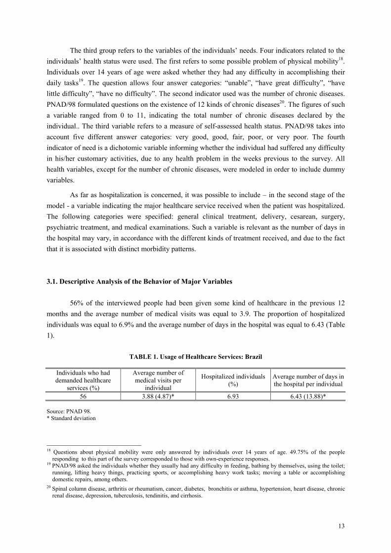
56% of the interviewed people had been given some kind of healthcare in the previous 12months and the average number of medical visits was equal to 3.9. The proportion of hospitalizedindividuals was equal to 6.9% and the average number of days in the hospital was equal to 6.43 (Table1).
TABLE 1. Usage of Healthcare Services: Brazil
Individuals who haddemanded healthcare
services (%)
Average number ofmedical visits per
individual
Hospitalized individuals(%)
Average number of days inthe hospital per individual
56 3.88 (4.87)* 6.93 6.43 (13.88)*
Source: PNAD 98.* Standard deviation
18 Questions about physical mobility were only answered by individuals over 14 years of age. 49.75% of the people
responding to this part of the survey corresponded to those with own-experience responses.19 PNAD/98 asked the individuals whether they usually had any difficulty in feeding, bathing by themselves, using the toilet;
running, lifting heavy things, practicing sports, or accomplishing heavy work tasks; moving a table or accomplishingdomestic repairs, among others.
20 Spinal column disease, arthritis or rheumatism, cancer, diabetes, bronchitis or asthma, hypertension, heart disease, chronicrenal disease, depression, tuberculosis, tendinitis, and cirrhosis.
14
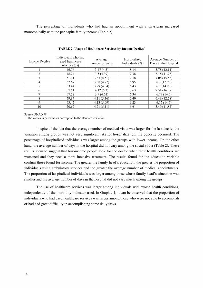
The percentage of individuals who had had an appointment with a physician increasedmonotonically with the per capita family income (Table 2).
TABLE 2. Usage of Healthcare Services by Income Deciles1
Income DecilesIndividuals who had
used healthcareservices (%)
Averagenumber of visits
HospitalizedIndividuals (%)
Average Number ofDays in the Hospital
1 46.76 3.47 (4,3) 8.14 5.78 (12.14)2 48.24 3.5 (4.39) 7.38 6.18 (11.76)3 51.11 3.63 (4.51) 7.18 7.08 (15.58)4 52.67 3.68 (4.72) 6.95 6.3 (12.92)5 53.44 3.79 (4.84) 6.43 6.7 (14.98)6 57.51 4.12 (5.3) 7.63 7.51 (16.87)7 57.52 3.9 (4.61) 6.34 6.77 (14.6)8 59.87 4.11 (5.36) 6.40 6.49 (12.78)9 63.42 4.13 (5.09) 6.23 6.17 (14.6)
10 70.62 4.21 (5.11) 6.61 5.40 (11.82)
Source: PNAD 98.1. The values in parentheses correspond to the standard deviation.
In spite of the fact that the average number of medical visits was larger for the last decile, thevariation among groups was not very significant. As for hospitalization, the opposite occurred. Thepercentage of hospitalized individuals was larger among the groups with lower income. On the otherhand, the average number of days in the hospital did not vary among the social strata (Table 2). Theseresults seem to suggest that low-income people look for the doctor when their health conditions areworsened and they need a more intensive treatment. The results found for the education variableconfirm those found for income. The greater the family head’s education, the greater the proportion ofindividuals using ambulatory services and the greater the average number of medical appointments.The proportion of hospitalized individuals was larger among those whose family head’s education wassmaller and the average number of days in the hospital did not vary much among the groups.
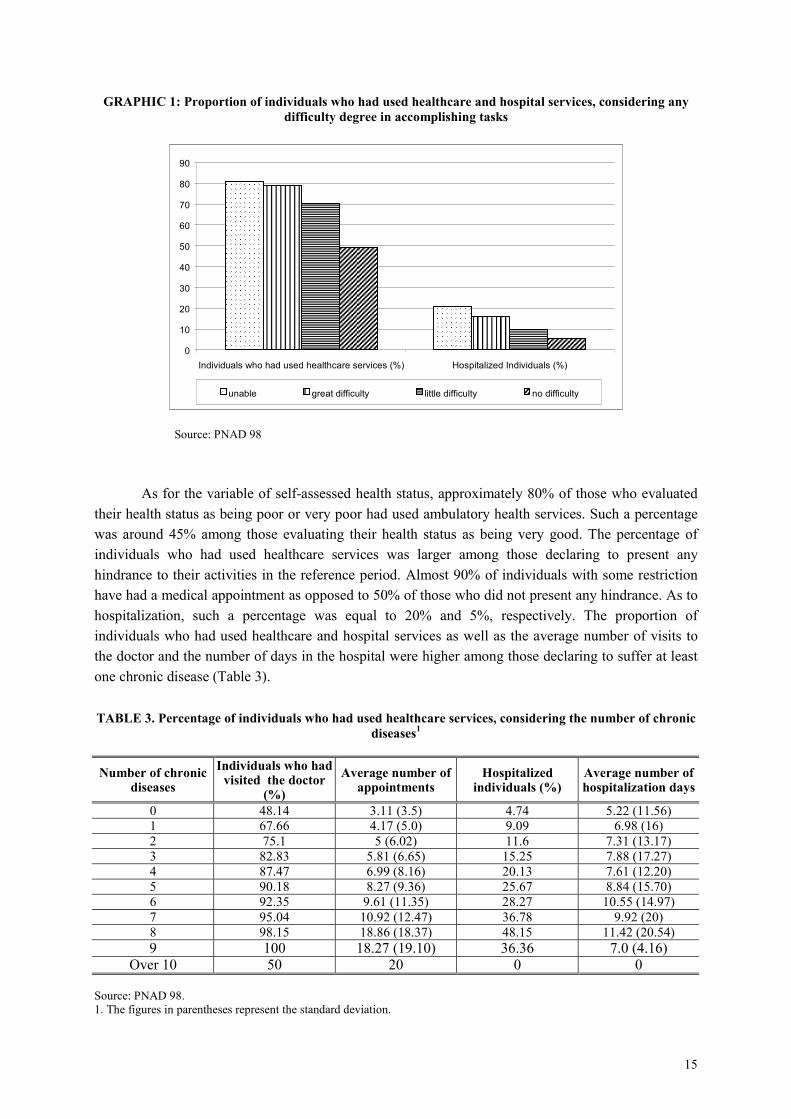
The use of healthcare services was larger among individuals with worse health conditions,independently of the morbidity indicator used. In Graphic 1, it can be observed that the proportion ofindividuals who had used healthcare services was larger among those who were not able to accomplishor had had great difficulty in accomplishing some daily tasks.
15
GRAPHIC 1: Proportion of individuals who had used healthcare and hospital services, considering anydifficulty degree in accomplishing tasks
0
10
20
30
40
50
60
70
80
90
Individuals who had used healthcare services (%) Hospitalized Individuals (%)
unable
great difficulty
little difficulty
no difficulty
Source: PNAD 98
As for the variable of self-assessed health status, approximately 80% of those who evaluatedtheir health status as being poor or very poor had used ambulatory health services. Such a percentagewas around 45% among those evaluating their health status as being very good. The percentage ofindividuals who had used healthcare services was larger among those declaring to present anyhindrance to their activities in the reference period. Almost 90% of individuals with some restrictionhave had a medical appointment as opposed to 50% of those who did not present any hindrance. As tohospitalization, such a percentage was equal to 20% and 5%, respectively. The proportion ofindividuals who had used healthcare and hospital services as well as the average number of visits tothe doctor and the number of days in the hospital were higher among those declaring to suffer at leastone chronic disease (Table 3).
TABLE 3. Percentage of individuals who had used healthcare services, considering the number of chronicdiseases1
Number of chronicdiseases
Individuals who hadvisited the doctor
(%)Average number of
appointmentsHospitalized
individuals (%)Average number ofhospitalization days
0 48.14 3.11 (3.5) 4.74 5.22 (11.56)1 67.66 4.17 (5.0) 9.09 6.98 (16)2 75.1 5 (6.02) 11.6 7.31 (13.17)3 82.83 5.81 (6.65) 15.25 7.88 (17.27)4 87.47 6.99 (8.16) 20.13 7.61 (12.20)5 90.18 8.27 (9.36) 25.67 8.84 (15.70)6 92.35 9.61 (11.35) 28.27 10.55 (14.97)7 95.04 10.92 (12.47) 36.78 9.92 (20)8 98.15 18.86 (18.37) 48.15 11.42 (20.54)9 100 18.27 (19.10) 36.36 7.0 (4.16)
Over 10 50 20 0 0
Source: PNAD 98.1. The figures in parentheses represent the standard deviation.
16
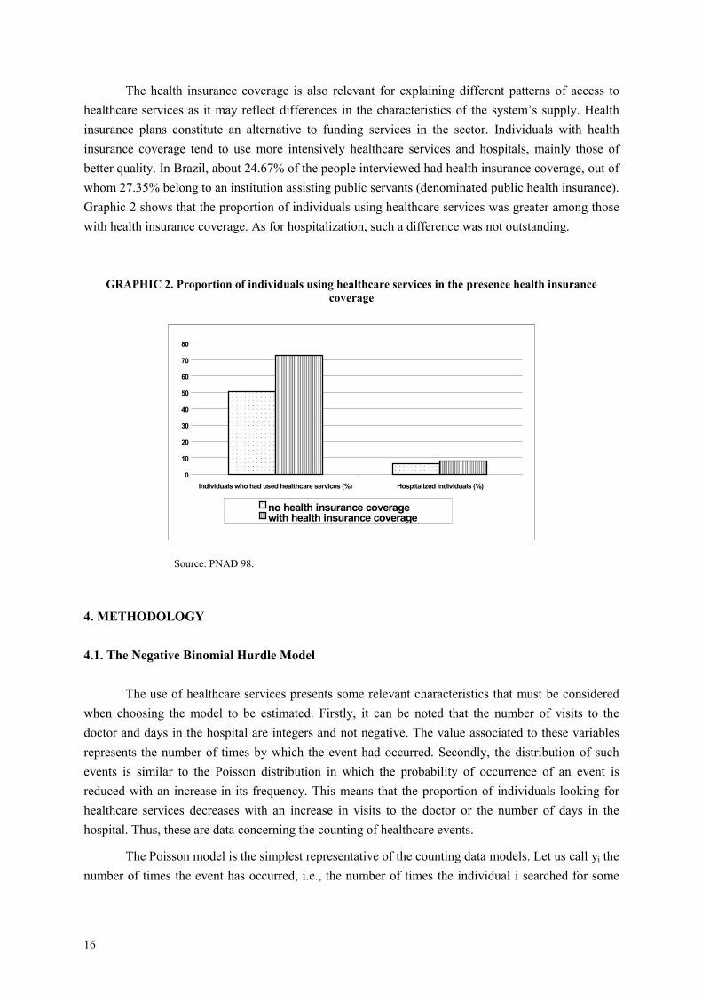
The health insurance coverage is also relevant for explaining different patterns of access tohealthcare services as it may reflect differences in the characteristics of the system’s supply. Healthinsurance plans constitute an alternative to funding services in the sector. Individuals with healthinsurance coverage tend to use more intensively healthcare services and hospitals, mainly those ofbetter quality. In Brazil, about 24.67% of the people interviewed had health insurance coverage, out ofwhom 27.35% belong to an institution assisting public servants (denominated public health insurance).Graphic 2 shows that the proportion of individuals using healthcare services was greater among thosewith health insurance coverage. As for hospitalization, such a difference was not outstanding.
GRAPHIC 2. Proportion of individuals using healthcare services in the presence health insurancecoverage
0
10
20
30
40
50
60
70
80
Individuals who had used healthcare services (%) Hospitalized Individuals (%)no health insurance coveragewith health insurance coverage
Source: PNAD 98.
4. METHODOLOGY
4.1. The Negative Binomial Hurdle Model
The use of healthcare services presents some relevant characteristics that must be consideredwhen choosing the model to be estimated. Firstly, it can be noted that the number of visits to thedoctor and days in the hospital are integers and not negative. The value associated to these variablesrepresents the number of times by which the event had occurred. Secondly, the distribution of suchevents is similar to the Poisson distribution in which the probability of occurrence of an event isreduced with an increase in its frequency. This means that the proportion of individuals looking forhealthcare services decreases with an increase in visits to the doctor or the number of days in thehospital. Thus, these are data concerning the counting of healthcare events.
The Poisson model is the simplest representative of the counting data models. Let us call yi thenumber of times the event has occurred, i.e., the number of times the individual i searched for some

17
healthcare service. This model asserts that each yi is extracted from the Poisson distribution with apositive intensive parameter µi. The probability that yi will occur N times is given by:
( )!
PrN
eNyNi
i
i µµ−
== , (1)
where i = 0,1,2,3,........individuals.
It is possible to include explaining variables when it is specified that the intensity parameter µi
is an exponential function of the covariant set:
∑= ij ijj Xb
i eµ > 0 (2)
where:
bj = j-th coefficient;
Xij = j-th explaining variable corresponding to i-th individual.
Thus, the following distribution of number of visits to the doctor or the number of days in thehospital (yi) is obtained, conditioned to the covariant vector Xi:
,...,2,1,0,!
)|( ==−
ii
yi
ii yy
exyfii µµ
(3)
The expected value of this function and the variance are given by:
[ ]
∑=== ij ijj Xb
iiiii exyVARxyE µ]|[| (4)
The Poisson model may become inadequate for the analysis of the use of healthcare servicesdue to some limitations. Firstly, this model assumes that the intensity parameter µis is deterministic.Generally speaking, such a supposition is not valid. As seen before, this parameter is a function of theobservable characteristics of individuals. However, there are some relevant characteristics which –being unobservable - are not included in the covariant vector. As it is not possible to model suchcharacteristics, it is necessary to include a random term in order to control the unobservedheterogeneity. If such a particularity is neglected, the model may present overdispersion, implying avariance greater than that assumed by the model. Secondly, the events are considered to beindependent in this model. In the case of visits to the doctor and days in the hospital, the probability ofa current appointment with the doctor may be related to previous visits.
An alternative to this is to use the negative binomial model, which is obtained by assuming
that the model intensity parameter has a stochastic component ive , where vi assumes a gammadistribution21. If the random component is included, the unobserved heterogeneity is taken intoaccount, as this term reflects the unobservable individuals’ characteristics.
21 See Cameron and Trivedi, 1998, pp.100-102. Gurmu (1997) showed that if there is a malspecification of unobserved
heterogeneity distribution, the estimates of parameters will be inconsistent. The author suggests an alternative method ofestimation based on semiparametric models. Such models do not impose a specific distribution for the unobservedheterogeneity component.
18
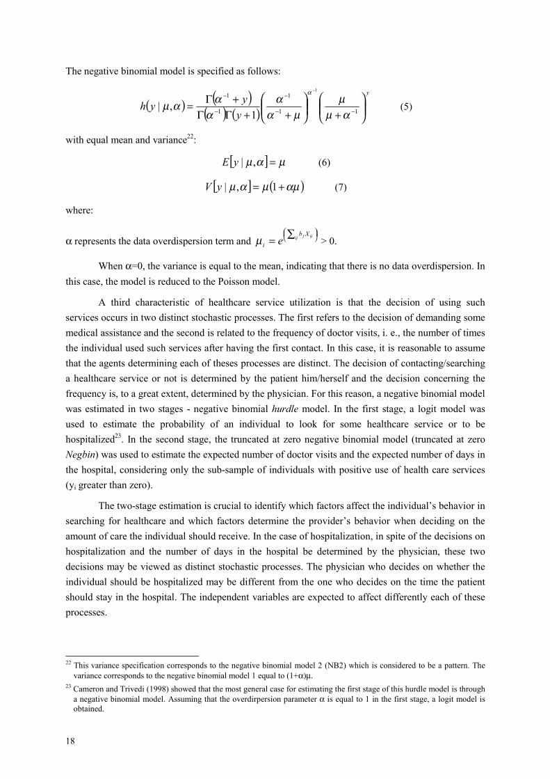
The negative binomial model is specified as follows:
( ) ( )( ) ( )
y
yyyh
+
++ΓΓ
+Γ= −−
−
−
−−
11
1
1
11
1,|
αµµ
µαα
αααµ
α
(5)
with equal mean and variance22:
[ ] µαµ =,|yE (6)
[ ] ( )αµµαµ += 1,|yV (7)
where:
α represents the data overdispersion term and
∑= ij ijj Xb
i eµ > 0.
When α=0, the variance is equal to the mean, indicating that there is no data overdispersion. Inthis case, the model is reduced to the Poisson model.
A third characteristic of healthcare service utilization is that the decision of using suchservices occurs in two distinct stochastic processes. The first refers to the decision of demanding somemedical assistance and the second is related to the frequency of doctor visits, i. e., the number of timesthe individual used such services after having the first contact. In this case, it is reasonable to assumethat the agents determining each of theses processes are distinct. The decision of contacting/searchinga healthcare service or not is determined by the patient him/herself and the decision concerning thefrequency is, to a great extent, determined by the physician. For this reason, a negative binomial modelwas estimated in two stages - negative binomial hurdle model. In the first stage, a logit model wasused to estimate the probability of an individual to look for some healthcare service or to behospitalized23. In the second stage, the truncated at zero negative binomial model (truncated at zeroNegbin) was used to estimate the expected number of doctor visits and the expected number of days inthe hospital, considering only the sub-sample of individuals with positive use of health care services(yi greater than zero).
The two-stage estimation is crucial to identify which factors affect the individual’s behavior insearching for healthcare and which factors determine the provider’s behavior when deciding on theamount of care the individual should receive. In the case of hospitalization, in spite of the decisions onhospitalization and the number of days in the hospital be determined by the physician, these twodecisions may be viewed as distinct stochastic processes. The physician who decides on whether theindividual should be hospitalized may be different from the one who decides on the time the patientshould stay in the hospital. The independent variables are expected to affect differently each of theseprocesses.
22 This variance specification corresponds to the negative binomial model 2 (NB2) which is considered to be a pattern. The
variance corresponds to the negative binomial model 1 equal to (1+α)µ.23 Cameron and Trivedi (1998) showed that the most general case for estimating the first stage of this hurdle model is through
a negative binomial model. Assuming that the overdirpersion parameter α is equal to 1 in the first stage, a logit model isobtained.

19
For the construction of a negative binomial hurdle, we specified two likelihood functionsparametrically independent, each representing a stage in the estimation procedure. Let us call yi thenumber of times an individual i looked for the doctor or the number of days of hospitalization, being yi
≥ 0 and let di be a binary variable which assumes a value equal to 1, when the medical contact isaccomplished, and zero when it is not . The likelihood function for the negative binomial hurdle model
HBNL may be specified as follows:
( ) ∏ ∏
Ω∈ Ω∈
−
≥×=−==
i i ii
iidii
dii
HBN xypr
xyprxyprxyprL ii
1 22'
22'
11'1
11'
,|1,|
,|01,|0αβ
αβαβαβ (8)
where:
i = 1, 2, 3, ... , individuals;
αs = overdispersion parameter of data in stages, being s = 1, 2;
Ω = whole sample;
Ω1 = subsample comprising only individuals who searched for some healthcare service.
The first likelihood function is based on the whole sample Ω, representing the binary processwhere the individual decides to contact the healthcare service or not. This process is determined by the
vector of parameters ( 11 ,αβ ) and estimated through a logit model:
[ ]
∑+==
ijij j Xb
ii
eXy
11
1|0Pr (9)
[ ]
∑+
∑==−
ijij j
ij ijj
Xb
Xb
ii
e
eXy1
1
1|0Pr1 (10)
The second likelihood function is the truncated at zero negative binomial model. This stage isbased only on the sample of individuals that have searched for some healthcare service (Ω1) andrepresents the probability that the number of visits to the doctor or hospitalization days be equal to yi,provided that a contact had been previously made. The following probability is obtained in this stage,
determined by the vector of parameters ( 22 ,αβ ):
[ ] ( )( ) ( ) ( )
iy
i
i
ii
iiii y
yyXy
+
−++ΓΓ+Γ
=≥ −
−
−
−
−
122
21
22
12
12
12
2 11
11
1,|Prαµ
µ
µααα
α
α
(11)
where:
∑= ij ijj Xb
i e 2
2µ > 0

20
The estimates of ( 11 ,αβ ) e ( 22,αβ ) are found as the two likelihood functions are separately
maximized. If the two processes are identical, i.e., if the two vectors of parameters are equal, theestimation is nested to the standard negative binomial model.
4.2. Specification Tests
We estimated the Poisson model, the negative binomial and the Poisson hurdle in order to testthe negative binomial hurdle model. Firstly, we performed the likelihood ratio test to certify whetherthe data were overdispersed24. The following hypotheses were tested:
Ho: α = 0H1: α > 0
The likelihood ratio test is obtained through the difference between the log-likelihood of thePoisson model and the negative binomial:
( )Negbinpoisson LNLNLR −−= 2 (12)
where:
LNpoisson = log- likelihood of the Poisson model;
LNNegbin = log-likelihood of the negative binomial model.
When α = 0, the negative binomial model is nested to Poisson model and the data are notoverdispersed. In this case, the statistics of the likelihood ratio test is equal to zero and the hypothesisHo is accepted.
Secondly, we tested the negative binomial model against the hurdle negative binomial in orderto verify whether the two decision-making processes (the contact decision and the frequency decision)are distinct. The likelihood ratio was used, so that we could test the following hypothesis:
Ho: β1 = β2
where:
βs = vector of parameters of stages, being s = 1,2.
In order to accomplish this test, we estimated the negative binomial model and the hurdlenegative binomial so as to obtain the respective log-likelihood. The likelihood ratio test is equal to:
( )[ ]truncadoNegbinitNegbin LNLNLNLR −+−= log2 (13)
24 When analyzing the data on frequency of medical visits and hospitalization days, we suspected that the data were
overdispersed, since the variance was greater than the mean. We applied the Lagrange multiplier test in order to certifywhether the overdispersion was maintained even after including regressors to the model. Another usual test in the literatureis that of Wald which is obtained by dividing the estimated value of α, divided by its standard error.
21
where:
LNNegbin = log-likelihood of the negative binomial model;
LNlogit = log-likelihood of the logit model (first stage);
LNNegbin-truncado = log-likelihood of the truncated at zero negative binomial model (second stage).
If the hypothesis Ho is validated, the hurdle model is reduced to the negative binomial.Thirdly, the Poisson hurdle model was tested against the negative binomial hurdle, by using thelikelihood ratio test. Accomplishing such a test is crucial as, when estimating the two stages, theoverdispersion of the data in the Poisson model can be eliminated.
4.3. Interpretation of Coefficients
In order to facilitate the interpretation of results, we present odds ratios, estimated by thelogistic model, and the marginal effects estimated by the truncated at zero negative binomial model.The odds ratios provide the percentage variation on the probability of the first contact with thehealthcare service by the individual due to an increase/reduction in an explaining variable. Forexample, if the odds ratio estimated for a discrete variable is equal to 1.20, this means that theprobability of an appointment with the doctor increases by 20% if the value of this variable isincreased in 1 unit. For the binary explaining variables, the odds ratios show the difference inprobability of medical visits in relation to the reference category. If the odds ratio estimated for abinary variable is equal to 0.20, the probability of one medical visit at least is 80% lower for thiscategory in relation to the reference group.
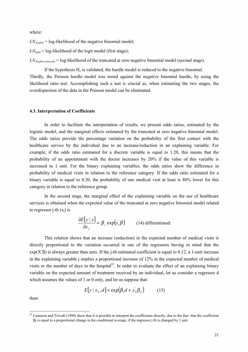
In the second stage, the marginal effect of the explaining variable on the use of healthcareservices is obtained when the expected value of the truncated at zero negative binomial model relatedto regressor j-th (xj) is
[ ] ( )ββ 'exp|ij
j
xx
xyE =∂
∂(14) differentiated:
This relation shows that an increase (reduction) in the expected number of medical visits isdirectly proportional to the variation occurred in one of the regressors having in mind that theexp(X’β) is always greater than zero. If the j-th estimated coefficient is equal to 0.12, a 1-unit increasein the explaining variable j implies a proportional increase of 12% in the expected number of medicalvisits or the number of days in the hospital25. In order to evaluate the effect of an explaining binaryvariable on the expected amount of treatment received by an individual, let us consider a regressor dwhich assumes the values of 1 or 0 only, and let us suppose that:
[ ] ( )2'212 exp,| ββ xddxyE += (15)
then:
25 Cameron and Trivedi (1998) show that it is possible to interpret the coefficients directly, due to the fact that the coefficient
βj is equal to a proportional change in the conditional average, if the regressor j th is changed by 1 unit.
22
[ ][ ]
( )( ) ( )1
2'2
2'21
2
2 expexp
exp,0|,1| β
βββ
=+
===
xx
xdyExdyE
(16)
Thus, the expected number of medical visits and days in the hospital (when the explainingvariable d is equal to 1) is exp(β1) times the expected number of medical visits and hospitalized days,when this variable is equal to zero. Such an effect, measured in percentage terms, is equal to [exp(ββββ)-1]*100. A result equal to 3.20 is saying that the expected number of medical visits is 3.20% higher fora category in relation to the reference category.
5. MAJOR RESULTS
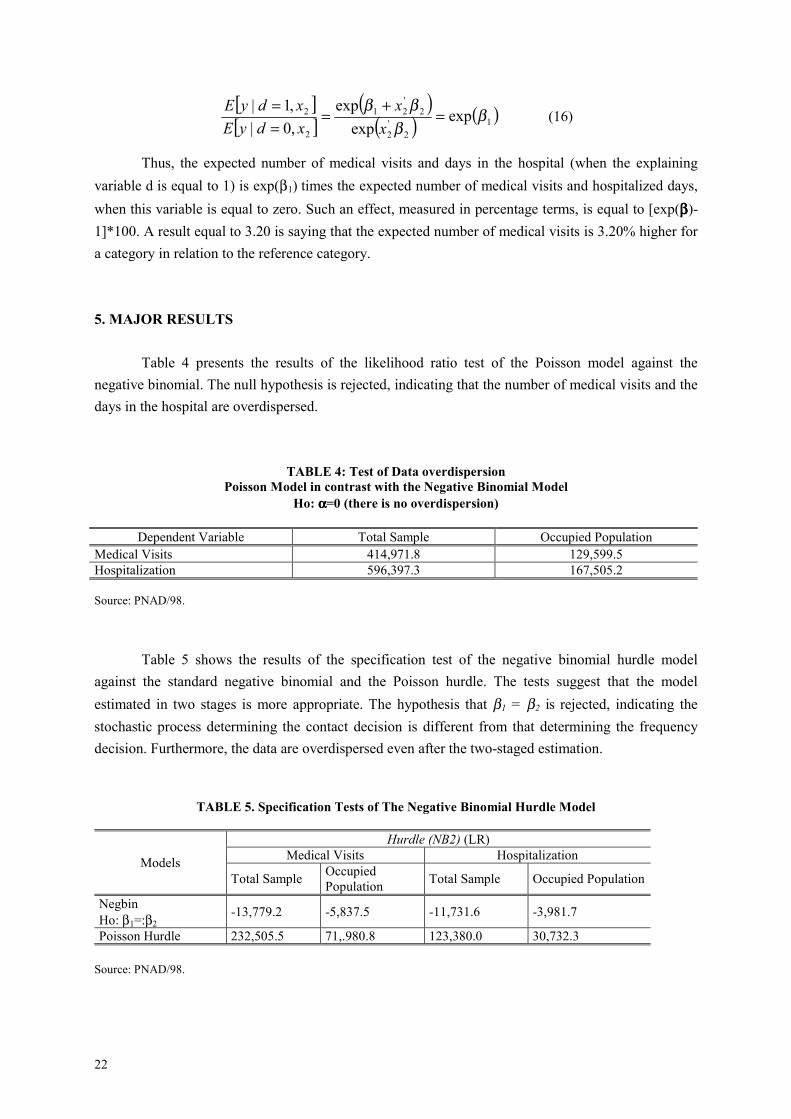
Table 4 presents the results of the likelihood ratio test of the Poisson model against thenegative binomial. The null hypothesis is rejected, indicating that the number of medical visits and thedays in the hospital are overdispersed.
TABLE 4: Test of Data overdispersionPoisson Model in contrast with the Negative Binomial Model
Ho: αααα=0 (there is no overdispersion)
Dependent Variable Total Sample Occupied PopulationMedical Visits 414,971.8 129,599.5Hospitalization 596,397.3 167,505.2
Source: PNAD/98.
Table 5 shows the results of the specification test of the negative binomial hurdle modelagainst the standard negative binomial and the Poisson hurdle. The tests suggest that the modelestimated in two stages is more appropriate. The hypothesis that β1 = β2 is rejected, indicating thestochastic process determining the contact decision is different from that determining the frequencydecision. Furthermore, the data are overdispersed even after the two-staged estimation.
TABLE 5. Specification Tests of The Negative Binomial Hurdle Model
Hurdle (NB2) (LR)Medical Visits HospitalizationModels
Total Sample OccupiedPopulation Total Sample Occupied Population
NegbinHo: β1=:β2
-13,779.2 -5,837.5 -11,731.6 -3,981.7
Poisson Hurdle 232,505.5 71,.980.8 123,380.0 30,732.3
Source: PNAD/98.
23
The analysis of major results is presented in the three following subsections which are dividedaccording to the variable groups previously defined26. We present the results found for ambulatoryservices and hospitalization. For each of these kinds of healthcare a model for the whole sample andanother for the occupied population at working age were estimated.
5.1. Is there social inequality in the access to healthcare services in Brazil?
The effect of socioeconomic variables on healthcare services is quite differentiated, dependingon the kind of service offered. The results reveal social inequality in the access to ambulatoryhealthcare services in Brazil in favor of more privileged socioeconomic groups, even if morbidity,occupational characteristics and health insurance coverage are controlled. For the inpatient care, themodel reveals social inequality in the access which is favorable to less privileged socioeconomicgroups. We also observed that the decision of seeing the doctor and the frequency of visits to aphysician were responsive to almost all occupational characteristics. The opposite occurs when thehospitalization model is analyzed. The number of worked hours is the only occupational variable thatis significant in the first stage estimation. In the second stage, no occupational variables are relevantfor explaining the number of days in the hospital.
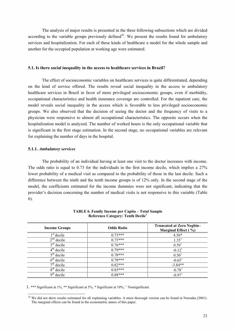
5.1.1. Ambulatory services
The probability of an individual having at least one visit to the doctor increases with income.The odds ratio is equal to 0.73 for the individuals in the first income decile, which implies a 27%lower probability of a medical visit as compared to the probability of those in the last decile. Such adifference between the ninth and the tenth income groups is of 12% only. In the second stage of themodel, the coefficients estimated for the income dummies were not significant, indicating that theprovider’s decision concerning the number of medical visits is not responsive to this variable (Table6).
TABLE 6. Family Income per Capita – Total SampleReference Category: Tenth Decile1
Income Groups Odds Ratio Truncated at Zero Negbin–Marginal Effect ( %)
1st decile 0.73*** 4.56*2nd decile 0.75*** 1.35+
3rd decile 0.76*** 0.59+
4th decile 0.79*** -0.12+
5th decile 0.78*** 0.50+
6th decile 0.78*** -0.65+
7th decile 0.82*** -3.84**8th decile 0.85*** -0.78+
9th decile 0.88*** -0.97+
1. *** Significant at 1%, ** Significant at 5%, * Significant at 10%, + Nonsignificant.
26 We did not show results estimated for all explaining variables. A more thorough version can be found in Noronha (2001).
The marginal effects can be found in the econometric annex of this paper.
24
Such a relation between income and access to ambulatory services in Brazil suggests that thebarrier encountered by low-income individuals is placed before the contact is made. The provider’sbehavior, no matter the funding source – public or private - , does not change with the patient’sincome, but it is the individual’s own behavior which is changed. Two hypotheses may be related tothis result. The first is concerned with the difference between the expected assistance among both thelow and high-income individuals. As they possess a health insurance coverage, the richer individualsalways expect to be assisted whenever searching for such services. The poorer individuals, on theother hand, generally show negative expectations about medical assistance, which make them give upsearching. Thus, even after controlling for the existence of health plans, richer individuals have betteraccess probably because they search for these services more intensively27. The expectation of notbeing assisted may reflect an unattended demand in the past. If he/she did not manage to be assistedwhen searching for healthcare services, the individual will prefer not to demand such services anymore as he/she expects not to be assisted again.
Another hypothesis is related to the opportunity cost for the people searching for healthcareservices which tends to be higher for lower-income classes. Generally speaking, time spent in linesand the cost of shifting to the place of medical assistance in relation to income are higher for the less-privileged socioeconomic groups. Furthermore, the way such income classes are inserted in the markettends to be more precarious, causing a certain employment instability and thus a higher opportunitycost for the search of such services.
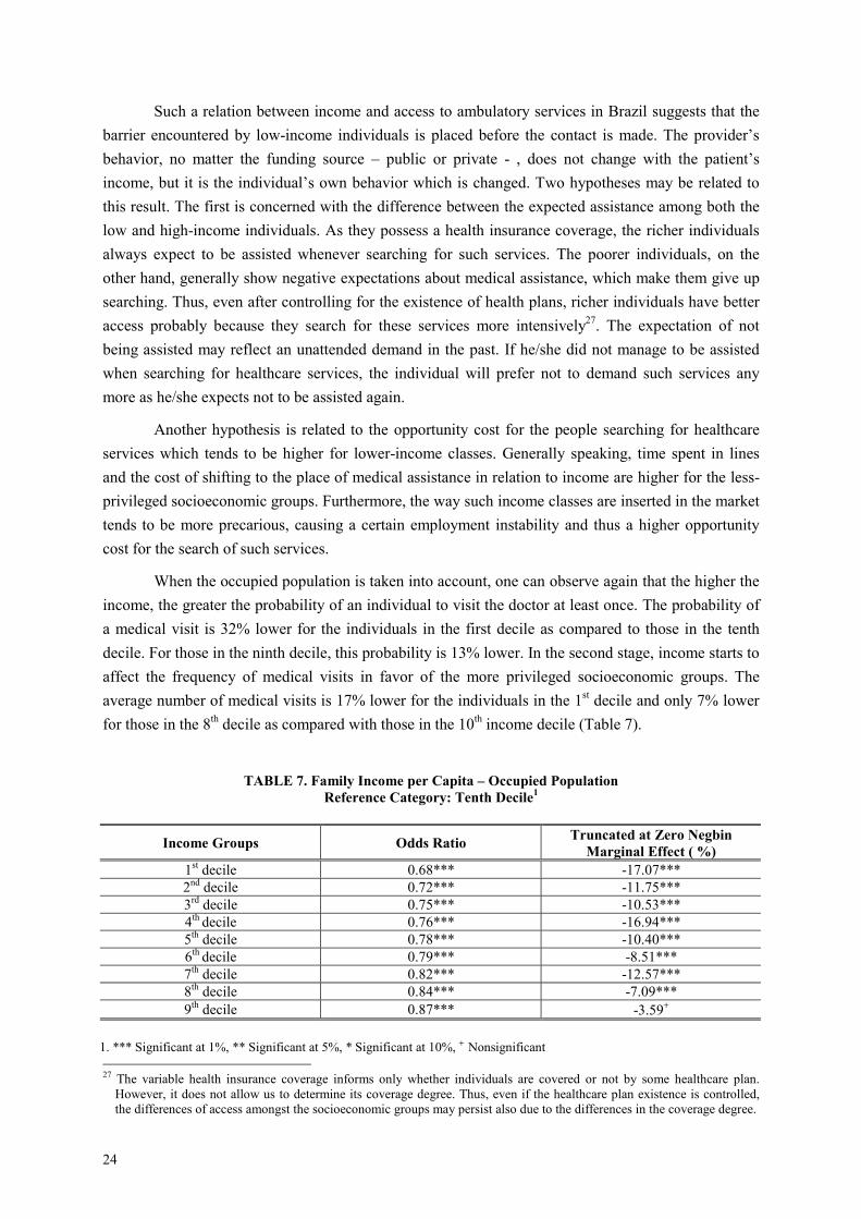
When the occupied population is taken into account, one can observe again that the higher theincome, the greater the probability of an individual to visit the doctor at least once. The probability ofa medical visit is 32% lower for the individuals in the first decile as compared to those in the tenthdecile. For those in the ninth decile, this probability is 13% lower. In the second stage, income starts toaffect the frequency of medical visits in favor of the more privileged socioeconomic groups. Theaverage number of medical visits is 17% lower for the individuals in the 1st decile and only 7% lowerfor those in the 8th decile as compared with those in the 10th income decile (Table 7).
TABLE 7. Family Income per Capita – Occupied PopulationReference Category: Tenth Decile1
Income Groups Odds Ratio Truncated at Zero NegbinMarginal Effect ( %)
1st decile 0.68*** -17.07***2nd decile 0.72*** -11.75***3rd decile 0.75*** -10.53***4th decile 0.76*** -16.94***5th decile 0.78*** -10.40***6th decile 0.79*** -8.51***7th decile 0.82*** -12.57***8th decile 0.84*** -7.09***9th decile 0.87*** -3.59+
1. *** Significant at 1%, ** Significant at 5%, * Significant at 10%, + Nonsignificant 27 The variable health insurance coverage informs only whether individuals are covered or not by some healthcare plan.
However, it does not allow us to determine its coverage degree. Thus, even if the healthcare plan existence is controlled,the differences of access amongst the socioeconomic groups may persist also due to the differences in the coverage degree.
25
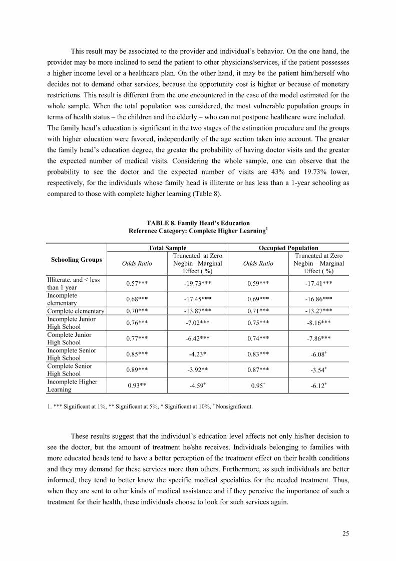
This result may be associated to the provider and individual’s behavior. On the one hand, theprovider may be more inclined to send the patient to other physicians/services, if the patient possessesa higher income level or a healthcare plan. On the other hand, it may be the patient him/herself whodecides not to demand other services, because the opportunity cost is higher or because of monetaryrestrictions. This result is different from the one encountered in the case of the model estimated for thewhole sample. When the total population was considered, the most vulnerable population groups interms of health status – the children and the elderly – who can not postpone healthcare were included.The family head’s education is significant in the two stages of the estimation procedure and the groupswith higher education were favored, independently of the age section taken into account. The greaterthe family head’s education degree, the greater the probability of having doctor visits and the greaterthe expected number of medical visits. Considering the whole sample, one can observe that theprobability to see the doctor and the expected number of visits are 43% and 19.73% lower,respectively, for the individuals whose family head is illiterate or has less than a 1-year schooling ascompared to those with complete higher learning (Table 8).
TABLE 8. Family Head’s EducationReference Category: Complete Higher Learning1
Total Sample Occupied Population
Schooling Groups Odds RatioTruncated at ZeroNegbin– Marginal
Effect ( %)Odds Ratio
Truncated at ZeroNegbin – Marginal
Effect ( %)Illiterate. and < lessthan 1 year 0.57*** -19.73*** 0.59*** -17.41***
Incompleteelementary 0.68*** -17.45*** 0.69*** -16.86***
Complete elementary 0.70*** -13.87*** 0.71*** -13.27***Incomplete JuniorHigh School 0.76*** -7.02*** 0.75*** -8.16***
Complete JuniorHigh School 0.77*** -6.42*** 0.74*** -7.86***
Incomplete SeniorHigh School 0.85*** -4.23* 0.83*** -6.08+
Complete SeniorHigh School 0.89*** -3.92** 0.87*** -3.54+
Incomplete HigherLearning 0.93** -4.59+ 0.95+ -6.12+
1. *** Significant at 1%, ** Significant at 5%, * Significant at 10%, + Nonsignificant.
These results suggest that the individual’s education level affects not only his/her decision tosee the doctor, but the amount of treatment he/she receives. Individuals belonging to families withmore educated heads tend to have a better perception of the treatment effect on their health conditionsand they may demand for these services more than others. Furthermore, as such individuals are betterinformed, they tend to better know the specific medical specialties for the needed treatment. Thus,when they are sent to other kinds of medical assistance and if they perceive the importance of such atreatment for their health, these individuals choose to look for such services again.
26
The family size is significant to explain the contact decision. The higher the number of familymembers, the smaller the probability that the individual have visited a doctor. In the second stage ofthe estimation this variable is significant only in the model for the whole sample. The expectednumber of medical visits is reduced by 3% to the extent that the family size is increased (Table 9).
TABLE 9. Family Size1
Estimated Models Odds Ratio Truncated at Zero Negbin–MarginalEffect ( %)
Total Sample 0.91*** -3.06***Occupied Population 0.97*** 0.02+
1. *** Significant at 1%, ** Significant at 5%, * Significant at 10%, + Nonsignificant.
A possible explanation for such a result is that, in a larger family, the parents have acquired abetter knowledge of their children’s care (learning by doing), taking less recourse to medical serviceswhen one of their children gets sick. In addition, the health expense share in the total budget may besmaller in larger families. Thus, even if family income per capita is controlled, the proportion ofhealthcare expenses may be reduced as the family size increases, implying a smaller utilization ofhealthcare services.
As for occupational characteristics, we observed that the probability of an individual visit tothe doctor is 14.41% greater for those working less than 40 weekly hours and the average number ofmedical visits is 2.99% higher. Such a result was expected, as the greater the individual’s working day,the greater his/her opportunity cost for searching some healthcare service.
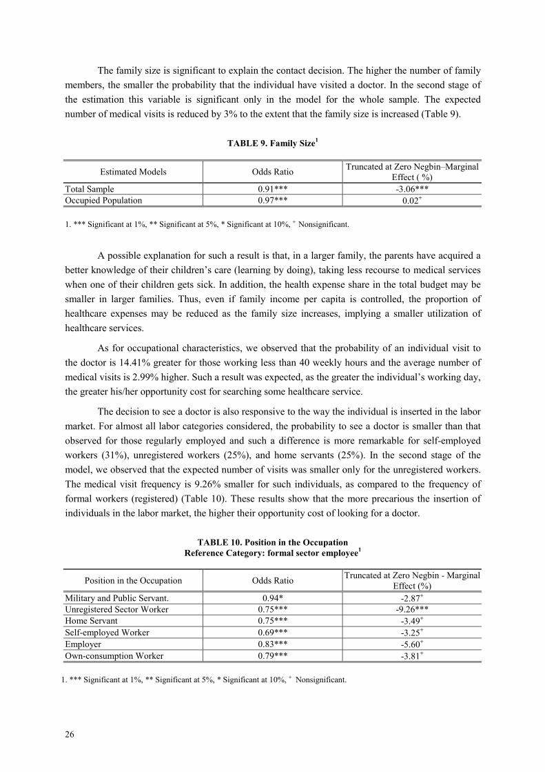
The decision to see a doctor is also responsive to the way the individual is inserted in the labormarket. For almost all labor categories considered, the probability to see a doctor is smaller than thatobserved for those regularly employed and such a difference is more remarkable for self-employedworkers (31%), unregistered workers (25%), and home servants (25%). In the second stage of themodel, we observed that the expected number of visits was smaller only for the unregistered workers.The medical visit frequency is 9.26% smaller for such individuals, as compared to the frequency offormal workers (registered) (Table 10). These results show that the more precarious the insertion ofindividuals in the labor market, the higher their opportunity cost of looking for a doctor.
TABLE 10. Position in the OccupationReference Category: formal sector employee1
Position in the Occupation Odds Ratio Truncated at Zero Negbin - MarginalEffect (%)
Military and Public Servant. 0.94* -2.87+
Unregistered Sector Worker 0.75*** -9.26***Home Servant 0.75*** -3.49+
Self-employed Worker 0.69*** -3.25+
Employer 0.83*** -5.60+
Own-consumption Worker 0.79*** -3.81+
1. *** Significant at 1%, ** Significant at 5%, * Significant at 10%, + Nonsignificant.
27
5.1.2. Inpatient Care
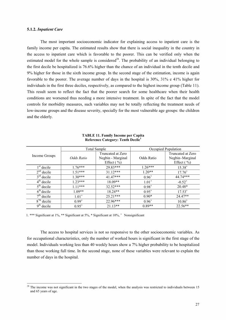
The most important socioeconomic indicator for explaining access to inpatient care is thefamily income per capita. The estimated results show that there is social inequality in the country inthe access to inpatient care which is favorable to the poorer. This can be verified only when theestimated model for the whole sample is considered28. The probability of an individual belonging tothe first decile be hospitalized is 76.6% higher than the chance of an individual in the tenth decile and9% higher for those in the sixth income group. In the second stage of the estimation, income is againfavorable to the poorer. The average number of days in the hospital is 30%, 31% e 41% higher forindividuals in the first three deciles, respectively, as compared to the highest income group (Table 11).This result seem to reflect the fact that the poorer search for some healthcare when their healthconditions are worsened thus needing a more intensive treatment. In spite of the fact that the modelcontrols for morbidity measures, such variables may not be totally reflecting the treatment needs oflow-income groups and the disease severity, specially for the most vulnerable age groups: the childrenand the elderly.
TABLE 11. Family Income per CapitaReference Category: Tenth Decile1
Total Sample Occupied Population
Income Groups Odds RatioTruncated at ZeroNegbin - Marginal
Effect ( %)Odds Ratio
Truncated at ZeroNegbin–Marginal
Effect ( %)1st decile 1.76*** 29.83*** 1.26*** 15.38+
2nd decile 1.51*** 31.12*** 1.20** 17.76+
3rd decile 1.30*** 41.47*** 0.96+ 44.74***4th decile 1.23*** 18.09** 1.01+ -0.52+
5th decile 1.11*** 32.52*** 0.98+ 20.48*6th decile 1.09** 18.24** 0.95+ 17.53+
7th decile 1.01+ 25.21*** 0.90* 24.47**8ºth decile 0.99+ 22.96*** 0.96+ 10.86+
9th decile 0.95+ 21.13** 0.89** 22.56**
1. *** Significant at 1%, ** Significant at 5%, * Significant at 10%, + Nonsignificant
The access to hospital services is not so responsive to the other socioeconomic variables. Asfor occupational characteristics, only the number of worked hours is significant in the first stage of themodel. Individuals working less than 40 weekly hours show a 7% higher probability to be hospitalizedthan those working full time. In the second stage, none of these variables were relevant to explain thenumber of days in the hospital.
28 The income was not significant in the two stages of the model, when the analysis was restricted to individuals between 15
and 65 years of age.

28
5.2. Access to healthcare services, according to the supply characteristics
5.2.1. Ambulatory services
Taking the estimated model for the whole sample into account, the probability of a medicalvisit is 91% larger for the individuals with a public healthcare institution plan and 139% higher forthose having some private health insurance coverage. In the second stage, the expected numbers ofmedical visits are 24.37% and 38.65% higher for individuals covered by healthcare plans provided bythe public and private sectors, respectively (Table 12).
TABLE 12. Supply Characteristics1
Total Sample Occupied Population
Variables Odds RatioNegbin Truncated at
Zero –MarginalEffect ( %)
Odds RatioNegbin Truncated at
Zero –MarginalEffect ( %)
Place of Residence –Reference category:Rural
1.21*** 17.63*** 1.08*** 0.95+
Public servant’shealthcare plan 1.91*** 24.37*** 1.90*** 25.61***
Private healthcareplan 2.39*** 38.65*** 2.39*** 41.60***
1. *** Significant at 1%, ** Significant at 5%, * Significant at 10%, + Nonsignificant.
The significance of such variable reflects a segmentation observed in the Brazilian healthcaresystem. Individuals covered by some healthcare plan have access to a wide variety of healthcareservices of good quality and at a low cost.
Living in an urban area affects the individual’s decision to see the doctor and the amount oftreatment he/she receives. In the two stages of the estimated model for the whole sample, individualsliving in urban areas show a 21% higher probability to visit the doctor and the expected number ofmedical visits is 17.63% higher (Table 12). This reflects the scarcity of such services in rural areas andindividuals living in the countryside will find greater difficulty in the access to some medicaltreatment. This variable is not significant for the occupied population.
5.2.2. Hospitalization services
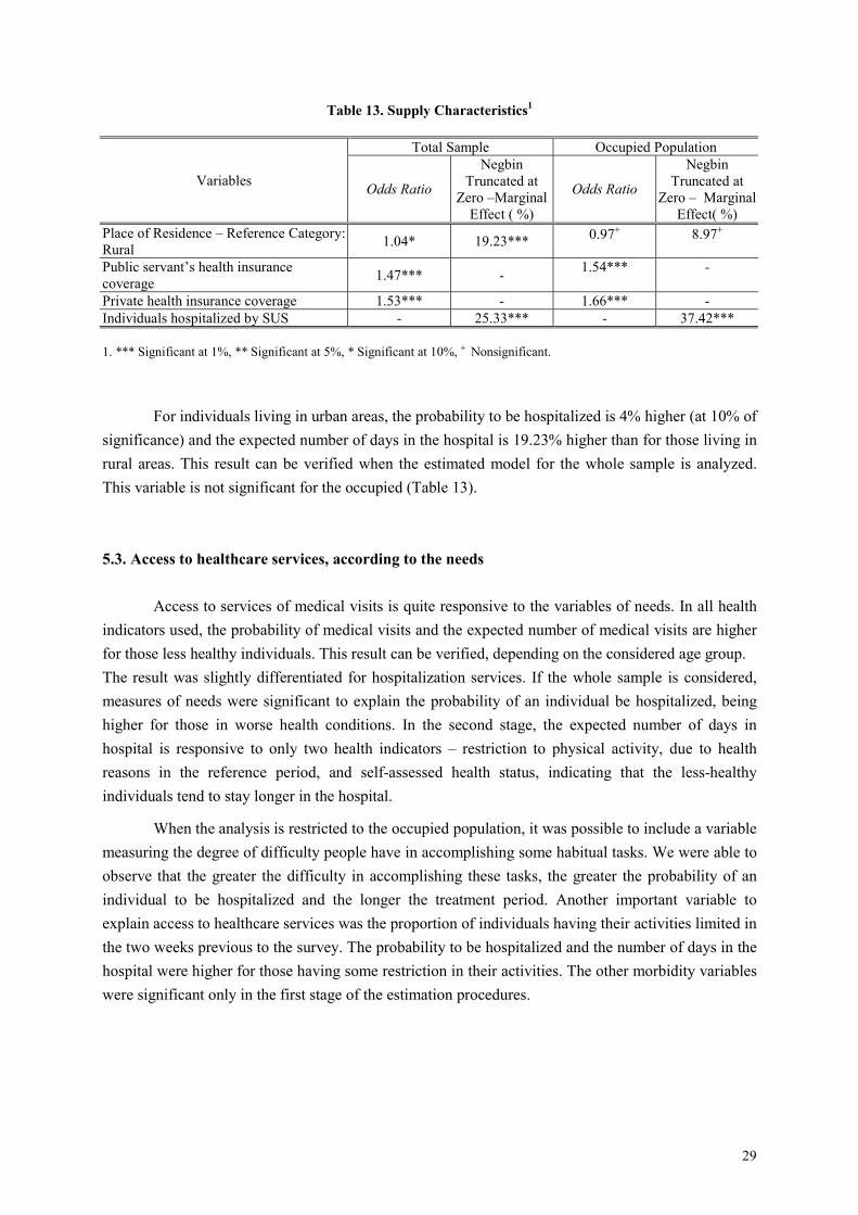
The estimated results for the whole sample show that the probability of hospitalization is 47%higher for those having some public healthcare plan and 53% higher for those with some privatehealthcare plan. In the second stage, we observed that the individuals hospitalized by SUS stayedlonger in the hospital and the expected number of days in the hospital being 25.33% higher (Table 13).This suggests that the insurance companies impose more stringent restrictions than SUS as for thenumber of days individuals must stay in the hospital for each accomplished medical procedure.
29
Table 13. Supply Characteristics1
Total Sample Occupied Population
Variables Odds Ratio
NegbinTruncated at
Zero –MarginalEffect ( %)
Odds Ratio
NegbinTruncated at
Zero – MarginalEffect( %)
Place of Residence – Reference Category:Rural 1.04* 19.23*** 0.97+ 8.97+
Public servant’s health insurancecoverage 1.47*** - 1.54*** -
Private health insurance coverage 1.53*** - 1.66*** -Individuals hospitalized by SUS - 25.33*** - 37.42***
1. *** Significant at 1%, ** Significant at 5%, * Significant at 10%, + Nonsignificant.
For individuals living in urban areas, the probability to be hospitalized is 4% higher (at 10% ofsignificance) and the expected number of days in the hospital is 19.23% higher than for those living inrural areas. This result can be verified when the estimated model for the whole sample is analyzed.This variable is not significant for the occupied (Table 13).
5.3. Access to healthcare services, according to the needs
Access to services of medical visits is quite responsive to the variables of needs. In all healthindicators used, the probability of medical visits and the expected number of medical visits are higherfor those less healthy individuals. This result can be verified, depending on the considered age group.The result was slightly differentiated for hospitalization services. If the whole sample is considered,measures of needs were significant to explain the probability of an individual be hospitalized, beinghigher for those in worse health conditions. In the second stage, the expected number of days inhospital is responsive to only two health indicators – restriction to physical activity, due to healthreasons in the reference period, and self-assessed health status, indicating that the less-healthyindividuals tend to stay longer in the hospital.
When the analysis is restricted to the occupied population, it was possible to include a variablemeasuring the degree of difficulty people have in accomplishing some habitual tasks. We were able toobserve that the greater the difficulty in accomplishing these tasks, the greater the probability of anindividual to be hospitalized and the longer the treatment period. Another important variable toexplain access to healthcare services was the proportion of individuals having their activities limited inthe two weeks previous to the survey. The probability to be hospitalized and the number of days in thehospital were higher for those having some restriction in their activities. The other morbidity variableswere significant only in the first stage of the estimation procedures.
30
6. FINAL REMARKS
The major contribution of this paper is its analysis of the social inequality in the access tohealthcare services in Brazil as two distinct stochastic processes. The estimation of the negativebinomial hurdle model is relevant, as it permits to evaluate whether the inequality in this market isrelated to the individuals’ behavior when demanding healthcare services or the doctor’s behavior whendeciding on the intensity of treatment the patient should receive.
The results encountered for ambulatory services show that there is inequality in the access tohealthcare services in Brazil, favoring the more privileged income groups. This result suggests that thebarrier found by the low-income individuals occurs even before any contact is established. Thevariables related to the occupational characteristics are also relevant to explain access to medicalassistance. The probability of seeing a doctor and the expected number of medical visits are smallerfor those individuals working full time than for those working less than 40 weekly hours. This findingis also observed for individuals whose insertion in the labor market is more precarious, mainly forthose working in the informal market, reflecting a higher opportunity cost that these people face whendemanding some healthcare service.
As for hospitalization services, we observed that the smaller the individual’s income, thegreater the probability of seeing a doctor. The frequency of medical visits is responsive to incomewhen the model is estimated for the whole sample, again favorable to the poorer groups.Such results, however, are not conclusive. There are still some restrictions found in the model whichneed to be evaluated so as to obtain more precise results. An extension of this paper would be toevaluate inequality in the access to healthcare services in Brazil, by considering some explainingvariables as being endogenous. An example of this is the self-assessed health status. People morefrequently assisted by a physician are better informed on their health status. Thus, they tend to betterevaluate their health status as compared to those not demanding such services. As a result, theassessment of health status depends on the use of healthcare services and these, in turn, are affected bythe individuals’ health status.
There are also two hypotheses posed by the negative binomial hurdle model which must betested. Firstly, the negative binomial model considers that the unobserved heterogeneity assumesgamma distribution. An alternative is to estimate the hurdle model for all the counting data of eventsby means of the semiparametric estimation method which does not impose a specific distribution forthe unobserved heterogeneity.
Another hypothesis of the hurdle model is that the individuals had only one disease eventduring the observation period considered in the database. Thus, the first count was equivalent to thefirst contact with the physician and the remaining counts were equivalent to medical visits related tothis very event. The problem concerning this hypothesis is that it may have occurred more than onedisease event implying multiple first contacts.
31
7. REFERENCES
ALBERTS, Jantina F., SANDERMAN, Robbert, EIMERS, Marietta, HEUVEL, Wim J. A. Van Den.Socioeconomic inequity in health care: a study of services utilization in Curaçao. Social Scienceand Medicine. vol. 45, n. 2, pp. 213-220, 1997.
ALMEIDA, Célia, TRAVASSOS, Cláudia, PORTO, Silvia and LABRA, Maria Eliana. Health sectorreform in Brazil: a case study of inequity. International Journal of Health Services, vol 30, no 1,2000.
CAMERON Cameron, A. C., TRIVEDI, P. K, MILNE, Frank, PIGGOTT, J. A microeconometricModel of the demand for health care and health Insurance in Australia. Review of EconomicsStudies. vol. 55, págs. 85-106, 1988.
CAMERON, Adrian Colin, TRIVEDI, Pravin K. Regression analysis of count data. Cambridge, UK ;New York, NY, USA: Cambridge University Press. 1998.
CAMPINO, Antonio Carlos Coelho et al. Poverty and Equity in Health in Latin America andCaribbean: Results of Country-Case Studies from Brazil, Ecuador, Guatemala, Jamaica, Mexico ePeru - Brazil. Washington; The World Bank (HNP-Health, Nutrition and Population), PNUD eOPAS, p. 1-82. 1999.
DOORSLAER, Eddy van, WAGSTAFF, Adam. Equity in the delivery of health care: someinternational comparisons. Journal of health Economics, vol. 11 (1992) pages: 389-411. NorthHolland.
DOORSLAER, Eddy van, et. al. Income – related inequalities in health: some internationalcomparisons. Journal of Health Economics, vol 16, p. 93-112, 1997.
GERDTHAM, Ulf-G. Equity in health care utilization: further tests based on hurdle models andswedish micro data. Health Economics, vol. 6, n. 3: 303-319. May - june, 1997. Chichester: JohnWiley.
GURMU, Shiferaw. Semi-parametric estimation of hurdle regression models with an application tomedicaid utilization. Journal of Applied Econometrics, vol.12, pgs. 225-242, 1997.
HECKMAN, J. J. Sample selection bias as a specification error. Econometrica, 47, 153-161. 1979.
LE GRAND, Julian. The distribution of public expendure: the case of health care. Economica, v.45, p.125-142, 1978.
MULLAHY, John. Specification and testing of some modified count data models. Journal ofEconometrics, vol. 33, p. 341-365, 1986.
NEWBOLD, K. Bruce, EYLES, John, BIRCH, Stephen. Equity in health care: methodologicalcontributions to the analysis of hospital utilization within Canada. Social Science Medicine. Vol40, n.9. 1995. Pgs. 1181-1192.
NORONHA, Kenya V. M. S. Dois Ensaios sobre a desigualdade social em saúde. 2001. 105 pgs.Dissertação de Mestrado (Mestrado em Economia). CEDEPLAR, UFMG, Belo Horizonte, 2001.
32
NORONHA, Kenya V.M.S. ANDRADE, Monica Viegas. Desigualdades Sociais em Saúde:evidências empíricas sobre o caso brasileiro. Revista Econômica do Nordeste, Fortaleza, vol. 32,n. especial, p. 877-897, nov. 2002.
PEREIRA, João. Prestação de cuidados de acordo com as necessidades? Um estudo empírico aplicadoao sistema de saúde português. In: PIOLA, Sérgio Francisco, VIANNA, Solon Magalhães (orgs).Economia da saúde: conceito e contribuição para a gestão da saúde. Brasília: IPEA, 1995.
POHLMEIER, Winfried., ULRICH, Volker. An Econometric Model of two-part decisionmakingprocess in the demand for health care. The Journal of Human Resources. Vol XXX no.2 pages:339-361. 1994.
TRAVASSOS, Cláudia, VIACAVA, Francisco, FERNANDES, Cristiano and ALMEIDA, CéliaMaria. Desigualdades geográficas e sociais na utilização de serviços de saúde no Brasil. Rio deJaneiro: Ciência e Saúde Coletiva. Vol 5 no1, jan-jul, 2000.
VIACAVA, Francisco, TRAVASSOS, Cláudia, PINHEIRO, Rejane, BRITO, Alexandre. Gênero eutilização de serviços de saúde no Brasil. (2001).
WATERS, Hugh R. Measuring equity um access to health care. Social Science and Medicine, vol. 51,2000.pages. 599-612.
33
ECONOMETRIC ANNEX
1. AMBULATORY SERVICES – ESTIMATED MODEL FOR TOTAL SAMPLE
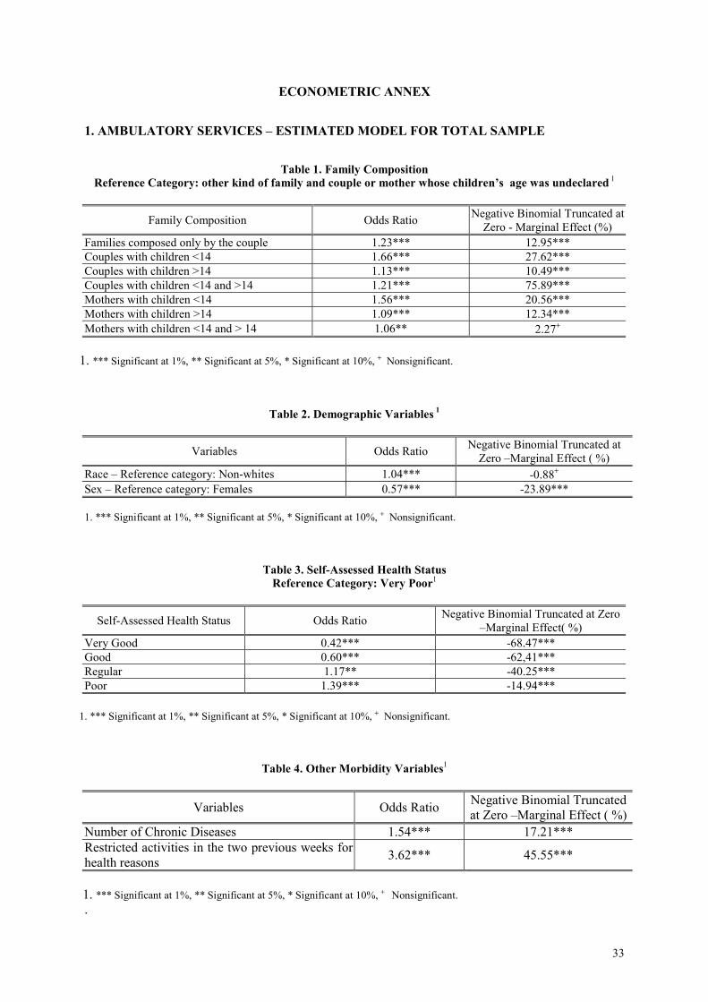
Table 1. Family CompositionReference Category: other kind of family and couple or mother whose children’s age was undeclared 1
Family Composition Odds Ratio Negative Binomial Truncated atZero - Marginal Effect (%)
Families composed only by the couple 1.23*** 12.95***Couples with children <14 1.66*** 27.62***Couples with children >14 1.13*** 10.49***Couples with children <14 and >14 1.21*** 75.89***Mothers with children <14 1.56*** 20.56***Mothers with children >14 1.09*** 12.34***Mothers with children <14 and > 14 1.06** 2.27+
1. *** Significant at 1%, ** Significant at 5%, * Significant at 10%, + Nonsignificant.
Table 2. Demographic Variables 1
Variables Odds Ratio Negative Binomial Truncated atZero –Marginal Effect ( %)
Race – Reference category: Non-whites 1.04*** -0.88+
Sex – Reference category: Females 0.57*** -23.89***
1. *** Significant at 1%, ** Significant at 5%, * Significant at 10%, + Nonsignificant.
Table 3. Self-Assessed Health StatusReference Category: Very Poor1
Self-Assessed Health Status Odds Ratio Negative Binomial Truncated at Zero–Marginal Effect( %)
Very Good 0.42*** -68.47***Good 0.60*** -62,41***Regular 1.17** -40.25***Poor 1.39*** -14.94***
1. *** Significant at 1%, ** Significant at 5%, * Significant at 10%, + Nonsignificant.
Table 4. Other Morbidity Variables1
Variables Odds Ratio Negative Binomial Truncatedat Zero –Marginal Effect ( %)
Number of Chronic Diseases 1.54*** 17.21***Restricted activities in the two previous weeks forhealth reasons 3.62*** 45.55***
1. *** Significant at 1%, ** Significant at 5%, * Significant at 10%, + Nonsignificant..
34
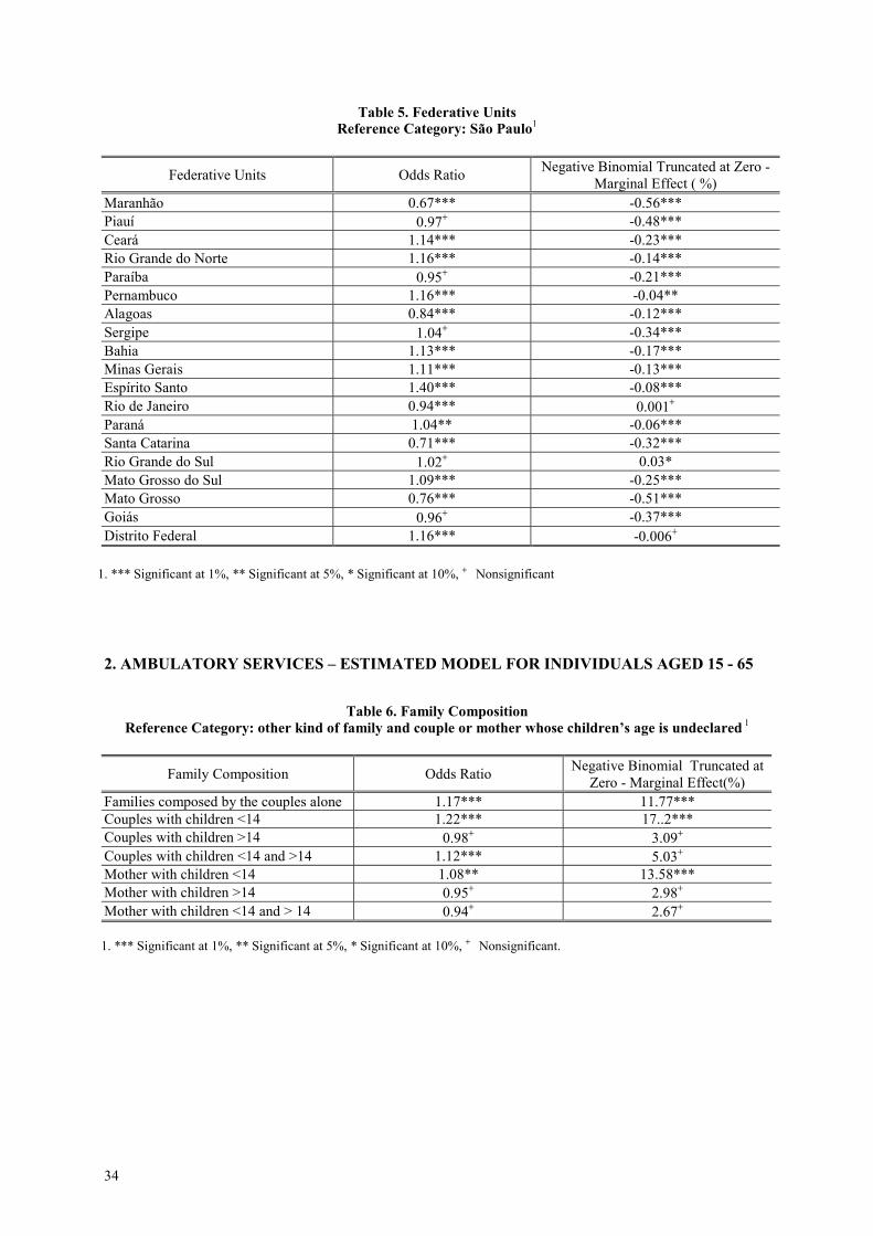
Table 5. Federative UnitsReference Category: São Paulo1
Federative Units Odds Ratio Negative Binomial Truncated at Zero -Marginal Effect ( %)
Maranhão 0.67*** -0.56***Piauí 0.97+ -0.48***Ceará 1.14*** -0.23***Rio Grande do Norte 1.16*** -0.14***Paraíba 0.95+ -0.21***Pernambuco 1.16*** -0.04**Alagoas 0.84*** -0.12***Sergipe 1.04+ -0.34***Bahia 1.13*** -0.17***Minas Gerais 1.11*** -0.13***Espírito Santo 1.40*** -0.08***Rio de Janeiro 0.94*** 0.001+
Paraná 1.04** -0.06***Santa Catarina 0.71*** -0.32***Rio Grande do Sul 1.02+ 0.03*Mato Grosso do Sul 1.09*** -0.25***Mato Grosso 0.76*** -0.51***Goiás 0.96+ -0.37***Distrito Federal 1.16*** -0.006+
1. *** Significant at 1%, ** Significant at 5%, * Significant at 10%, + Nonsignificant
2. AMBULATORY SERVICES – ESTIMATED MODEL FOR INDIVIDUALS AGED 15 - 65
Table 6. Family CompositionReference Category: other kind of family and couple or mother whose children’s age is undeclared 1
Family Composition Odds Ratio Negative Binomial Truncated atZero - Marginal Effect(%)
Families composed by the couples alone 1.17*** 11.77***Couples with children <14 1.22*** 17..2***Couples with children >14 0.98+ 3.09+
Couples with children <14 and >14 1.12*** 5.03+
Mother with children <14 1.08** 13.58***Mother with children >14 0.95+ 2.98+
Mother with children <14 and > 14 0.94+ 2.67+
1. *** Significant at 1%, ** Significant at 5%, * Significant at 10%, + Nonsignificant.
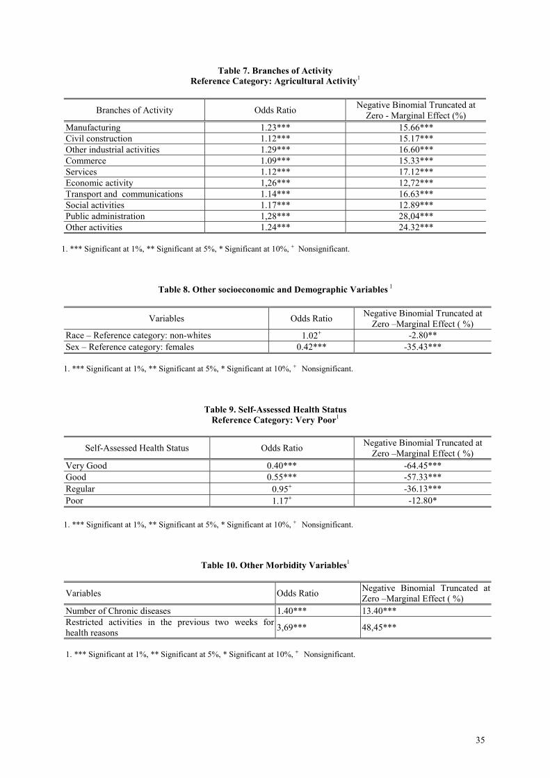
35
Table 7. Branches of ActivityReference Category: Agricultural Activity1
Branches of Activity Odds Ratio Negative Binomial Truncated atZero - Marginal Effect (%)
Manufacturing 1.23*** 15.66***Civil construction 1.12*** 15.17***Other industrial activities 1.29*** 16.60***Commerce 1.09*** 15.33***Services 1.12*** 17.12***Economic activity 1,26*** 12,72***Transport and communications 1.14*** 16.63***Social activities 1.17*** 12.89***Public administration 1,28*** 28,04***Other activities 1.24*** 24.32***
1. *** Significant at 1%, ** Significant at 5%, * Significant at 10%, + Nonsignificant.
Table 8. Other socioeconomic and Demographic Variables 1
Variables Odds Ratio Negative Binomial Truncated atZero –Marginal Effect ( %)
Race – Reference category: non-whites 1.02+ -2.80**Sex – Reference category: females 0.42*** -35.43***
1. *** Significant at 1%, ** Significant at 5%, * Significant at 10%, + Nonsignificant.
Table 9. Self-Assessed Health StatusReference Category: Very Poor1
Self-Assessed Health Status Odds Ratio Negative Binomial Truncated atZero –Marginal Effect ( %)
Very Good 0.40*** -64.45***Good 0.55*** -57.33***Regular 0.95+ -36.13***Poor 1.17+ -12.80*
1. *** Significant at 1%, ** Significant at 5%, * Significant at 10%, + Nonsignificant.
Table 10. Other Morbidity Variables1
Variables Odds Ratio Negative Binomial Truncated atZero –Marginal Effect ( %)
Number of Chronic diseases 1.40*** 13.40***Restricted activities in the previous two weeks forhealth reasons 3,69*** 48,45***
1. *** Significant at 1%, ** Significant at 5%, * Significant at 10%, + Nonsignificant.
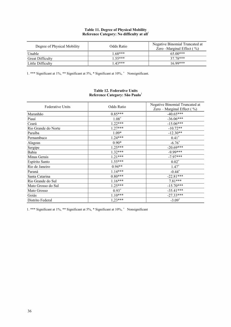
36
Table 11. Degree of Physical MobilityReference Category: No difficulty at all1
Degree of Physical Mobility Odds Ratio Negative Binomial Truncated atZero –Marginal Effect ( %)
Unable 1.68*** 65.00***Great Difficulty 1.55*** 37.78***Little Difficulty 1.43*** 16.99***
1. *** Significant at 1%, ** Significant at 5%, * Significant at 10%, + Nonsignificant.
Table 12. Federative UnitsReference Category: São Paulo1
Federative Units Odds Ratio Negative Binomial Truncated atZero – Marginal Effect ( %)
Maranhão 0.85*** -40.65***Piauí 1.08+ -36.06***Ceará 1.22*** -15.06***Rio Grande do Norte 1.27*** -10.72**Paraíba 1.09* -12.30**Pernambuco 1.24*** 0.41+
Alagoas 0.90* -6.76+
Sergipe 1.25*** -20.69***Bahia 1.32*** -9.99***Minas Gerais 1.21*** -7.97***Espírito Santo 1.55*** 0.02+
Rio de Janeiro 0.94** 1.47+
Paraná 1.14*** -0.44+
Santa Catarina 0.80*** -22.81***Rio Grande do Sul 1.16*** 7.81***Mato Grosso do Sul 1.25*** -15.70***Mato Grosso 0.93+ -35.41***Goiás 1.10*** -27.33***Distrito Federal 1,23*** -3.09+
1. *** Significant at 1%, ** Significant at 5%, * Significant at 10%, + Nonsignificant
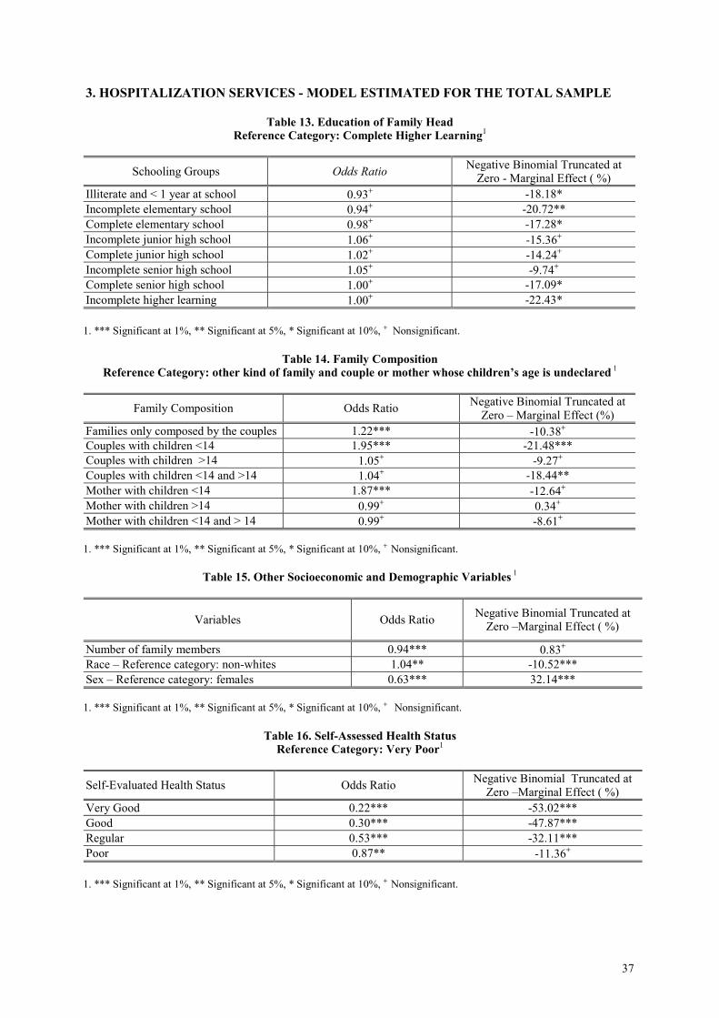
37
3. HOSPITALIZATION SERVICES - MODEL ESTIMATED FOR THE TOTAL SAMPLE
Table 13. Education of Family HeadReference Category: Complete Higher Learning1
Schooling Groups Odds Ratio Negative Binomial Truncated atZero - Marginal Effect ( %)
Illiterate and < 1 year at school 0.93+ -18.18*Incomplete elementary school 0.94+ -20.72**Complete elementary school 0.98+ -17.28*Incomplete junior high school 1.06+ -15.36+
Complete junior high school 1.02+ -14.24+
Incomplete senior high school 1.05+ -9.74+
Complete senior high school 1.00+ -17.09*Incomplete higher learning 1.00+ -22.43*
1. *** Significant at 1%, ** Significant at 5%, * Significant at 10%, + Nonsignificant.
Table 14. Family CompositionReference Category: other kind of family and couple or mother whose children’s age is undeclared 1
Family Composition Odds Ratio Negative Binomial Truncated atZero – Marginal Effect (%)
Families only composed by the couples 1.22*** -10.38+
Couples with children <14 1.95*** -21.48***Couples with children >14 1.05+ -9.27+
Couples with children <14 and >14 1.04+ -18.44**Mother with children <14 1.87*** -12.64+
Mother with children >14 0.99+ 0.34+
Mother with children <14 and > 14 0.99+ -8.61+
1. *** Significant at 1%, ** Significant at 5%, * Significant at 10%, + Nonsignificant.
Table 15. Other Socioeconomic and Demographic Variables 1
Variables Odds Ratio Negative Binomial Truncated atZero –Marginal Effect ( %)
Number of family members 0.94*** 0.83+
Race – Reference category: non-whites 1.04** -10.52***Sex – Reference category: females 0.63*** 32.14***
1. *** Significant at 1%, ** Significant at 5%, * Significant at 10%, + Nonsignificant.
Table 16. Self-Assessed Health StatusReference Category: Very Poor1
Self-Evaluated Health Status Odds Ratio Negative Binomial Truncated atZero –Marginal Effect ( %)
Very Good 0.22*** -53.02***Good 0.30*** -47.87***Regular 0.53*** -32.11***Poor 0.87** -11.36+
1. *** Significant at 1%, ** Significant at 5%, * Significant at 10%, + Nonsignificant.
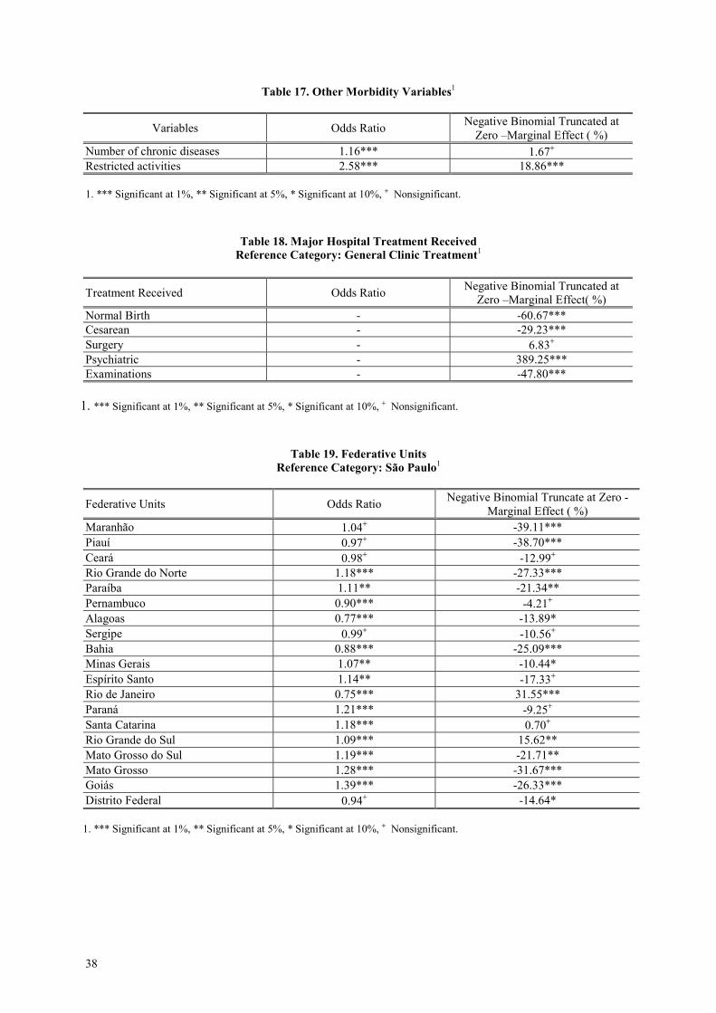
38
Table 17. Other Morbidity Variables1
Variables Odds Ratio Negative Binomial Truncated atZero –Marginal Effect ( %)
Number of chronic diseases 1.16*** 1.67+
Restricted activities 2.58*** 18.86***
1. *** Significant at 1%, ** Significant at 5%, * Significant at 10%, + Nonsignificant.
Table 18. Major Hospital Treatment ReceivedReference Category: General Clinic Treatment1
Treatment Received Odds Ratio Negative Binomial Truncated atZero –Marginal Effect( %)
Normal Birth - -60.67***Cesarean - -29.23***Surgery - 6.83+
Psychiatric - 389.25***Examinations - -47.80***
1. *** Significant at 1%, ** Significant at 5%, * Significant at 10%, + Nonsignificant.
Table 19. Federative UnitsReference Category: São Paulo1
Federative Units Odds Ratio Negative Binomial Truncate at Zero -Marginal Effect ( %)
Maranhão 1.04+ -39.11***Piauí 0.97+ -38.70***Ceará 0.98+ -12.99+
Rio Grande do Norte 1.18*** -27.33***Paraíba 1.11** -21.34**Pernambuco 0.90*** -4.21+
Alagoas 0.77*** -13.89*Sergipe 0.99+ -10.56+
Bahia 0.88*** -25.09***Minas Gerais 1.07** -10.44*Espírito Santo 1.14** -17.33+
Rio de Janeiro 0.75*** 31.55***Paraná 1.21*** -9.25+
Santa Catarina 1.18*** 0.70+
Rio Grande do Sul 1.09*** 15.62**Mato Grosso do Sul 1.19*** -21.71**Mato Grosso 1.28*** -31.67***Goiás 1.39*** -26.33***Distrito Federal 0.94+ -14.64*
1. *** Significant at 1%, ** Significant at 5%, * Significant at 10%, + Nonsignificant.
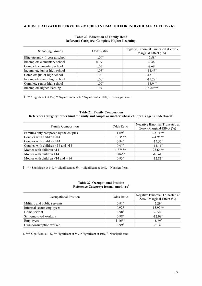
39
4. HOSPITALIZATION SERVICES - MODEL ESTIMATED FOR INDIVIDUALS AGED 15 - 65
Table 20. Education of Family HeadReference Category: Complete Higher Learning1
Schooling Groups Odds Ratio Negative Binomial Truncated at Zero -Marginal Effect ( %)
Illiterate and < 1 year at school 1.00+ -2.58+
Incomplete elementary school 0.97+ -9.48+
Complete elementary school 1.03+ -2.69+
Incomplete junior high school 1.05+ -14.43+
Complete junior high school 1.08+ -13.13+
Incomplete senior high school 1.00+ -15.29+
Complete senior high school 1.09+ -13.94+
Incomplete higher learning 1.04+ -33.20***
1. *** Significant at 1%, ** Significant at 5%, * Significant at 10%, + Nonsignificant.
Table 21. Family CompositionReference Category: other kind of family and couple or mother whose children’s age is undeclared 1
Family Composition Odds Ratio Negative Binomial Truncated atZero - Marginal Effect (%)
Families only composed by the couples 1.09+ -25.71**Couples with children <14 1.63*** -24.95**Couples with children >14 0.94+ -15.52+
Couples with children <14 and >14 0.97+ -11.11+
Mother with children <14 1.87*** -25.64**Mother with children >14 0.84** -16.41+
Mother with children <14 and > 14 0.93+ -12.81+
1. *** Significant at 1%, ** Significant at 5%, * Significant at 10%, + Nonsignificant.
Table 22. Occupational PositionReference Category: formal employee1
Occupational Position Odds Ratio Negative Binomial Truncated atZero - Marginal Effect (%)
Military and public servants 0.91+ -7.29+
Informal sector employees 0.92* -15.92**Home servant 0.98+ -9.50+
Self-employed workers 0.98+ -12.99+
Employers 1.16** 18.89+
Own-consumption worker 0.99+ -3.14+
1. *** Significant at 1%, ** Significant at 5%, * Significant at 10%, + Nonsignificant.
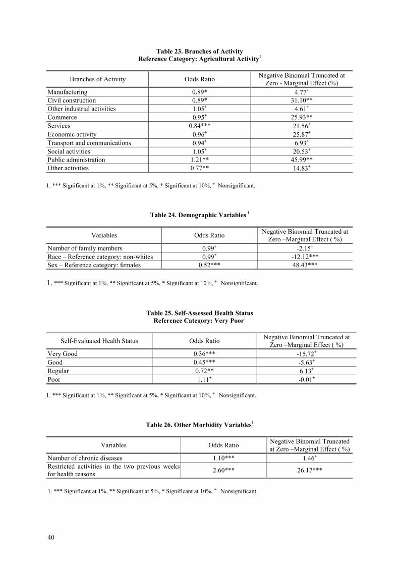
40
Table 23. Branches of ActivityReference Category: Agricultural Activity1
Branches of Activity Odds Ratio Negative Binomial Truncated atZero - Marginal Effect (%)
Manufacturing 0.89* 4.77+
Civil construction 0.89* 31.10**Other industrial activities 1.05+ 4.61+
Commerce 0.95+ 25.93**Services 0.84*** 21.56+
Economic activity 0.96+ 25.87+
Transport and communications 0.94+ 6.93+
Social activities 1.05+ 20.53+
Public administration 1.21** 45.99**Other activities 0.77** 14.83+
1. *** Significant at 1%, ** Significant at 5%, * Significant at 10%, + Nonsignificant.
Table 24. Demographic Variables 1
Variables Odds Ratio Negative Binomial Truncated atZero –Marginal Effect ( %)
Number of family members 0.99+ -2.15+
Race – Reference category: non-whites 0.99+ -12.12***Sex – Reference category: females 0.52*** 48.43***
1. *** Significant at 1%, ** Significant at 5%, * Significant at 10%, + Nonsignificant.
Table 25. Self-Assessed Health StatusReference Category: Very Poor1
Self-Evaluated Health Status Odds Ratio Negative Binomial Truncated atZero –Marginal Effect ( %)
Very Good 0.36*** -15.72+
Good 0.45*** -5.63+
Regular 0.72** 6.13+
Poor 1.11+ -0.01+
1. *** Significant at 1%, ** Significant at 5%, * Significant at 10%, + Nonsignificant.
Table 26. Other Morbidity Variables1
Variables Odds Ratio Negative Binomial Truncatedat Zero –Marginal Effect ( %)
Number of chronic diseases 1.10*** 1.46+
Restricted activities in the two previous weeksfor health reasons 2.60*** 26.17***
1. *** Significant at 1%, ** Significant at 5%, * Significant at 10%, + Nonsignificant.
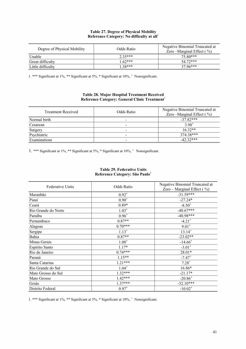
41
Table 27. Degree of Physical MobilityReference Category: No difficulty at all1
Degree of Physical Mobility Odds Ratio Negative Binomial Truncated atZero –Marginal Effect ( %)
Unable 2.35*** 75.80***Great difficulty 1.62*** 54.72***Little difficulty 1.38*** 37.96***
1. *** Significant at 1%, ** Significant at 5%, * Significant at 10%, + Nonsignificant.
Table 28. Major Hospital Treatment ReceivedReference Category: General Clinic Treatment1
Treatment Received Odds Ratio Negative Binomial Truncated atZero –Marginal Effect ( %)
Normal birth - -37.82***Cesarean - 3.98+
Surgery - 16.32**Psychiatric - 374.38***Examinations - -42.32***
1. *** Significant at 1%, ** Significant at 5%, * Significant at 10%, + Nonsignificant.
Table 29. Federative UnitsReference Category: São Paulo1
Federative Units Odds Ratio Negative Binomial Truncated atZero – Marginal Effect ( %)
Maranhão 0.92+ -31.59***Piauí 0.90+ -27.24*Ceará 0.89* -8.50+
Rio Grande do Norte 1.03+ -40.67***Paraíba 0.96+ -40.98***Pernambuco 0.87** -4.21+
Alagoas 0.70*** 9.01+
Sergipe 1.13+ 13.14+
Bahia 0.87** -23.02**Minas Gerais 1.00+ -14.66+
Espírito Santo 1.17* -3.01+
Rio de Janeiro 0.74*** 28.01*Paraná 1.15** -7.47+
Santa Catarina 1.21*** 7.28+
Rio Grande do Sul 1.04+ 16.86*Mato Grosso do Sul 1.32*** -21.17*Mato Grosso 1.42*** -20.86+
Goiás 1.37*** -32.10***Distrito Federal 0.97+ -10.02+
1. *** Significant at 1%, ** Significant at 5%, * Significant at 10%, + Nonsignificant.