Embed Size (px)
Citation preview

arX
iv:0
810.
1737
v1 [
hep-
th]
10
Oct
200
8
arXiv:0810.1737
MIT-CTP-3990
UT-Komaba/08-14
IPMU 08-0074
The boundary state from open string fields
Michael Kiermaier1,2, Yuji Okawa3 and Barton Zwiebach1
1 Center for Theoretical Physics
Massachusetts Institute of Technology
Cambridge, MA 02139, USA
[email protected], [email protected]
2 Institute for the Physics and Mathematics of the Universe
University of Tokyo
Kashiwa, Chiba 277-8582, Japan
3 Institute of Physics, University of Tokyo
Komaba, Meguro-ku, Tokyo 153-8902, Japan
Abstract
We construct a class of BRST-invariant closed string states for any classical solution of open
string field theory. The closed string state is a nonlinear functional of the open string field
and changes by a BRST-exact term under a gauge transformation of the solution. As a result,
its contraction with an on-shell closed string state provides a gauge-invariant observable of
open string field theory. Unlike previously known observables, however, the contraction with
off-shell closed string states in the Fock space is well defined and regular. Moreover, we claim
that the BRST-invariant closed string state coincides, up to a possible BRST-exact term, with
the boundary state of the boundary conformal field theory which the solution is expected to
describe. Our construction requires a choice of a propagator strip. If we choose the Schnabl
propagator strip, the BRST-invariant state becomes explicitly calculable. We calculate it for
various known analytic solutions of open string field theory and, remarkably, we find that it
precisely coincides with the boundary state without any additional BRST-exact term. Our re-
sults imply, in particular, that the wildly oscillatory rolling tachyon solution of open string field
theory actually describes the regular closed string physics studied by Sen using the boundary
state.

Contents
1 Introduction 2
2 Half-propagator strips and closed string states 6
2.1 Half-propagator strips for regular linear b-gauges . . . . . . . . . . . . . . . . . . 6
2.2 Star multiplication of half-propagator strips . . . . . . . . . . . . . . . . . . . . 10
2.3 Closed string states from half-propagator strips . . . . . . . . . . . . . . . . . . 13
3 Construction of BRST-invariant closed string states 15
3.1 The boundary state from the half-propagator strip . . . . . . . . . . . . . . . . . 16
3.2 Construction of the closed string state |B∗(Ψ)〉 . . . . . . . . . . . . . . . . . . . 16
3.3 BRST invariance of |B∗(Ψ)〉 . . . . . . . . . . . . . . . . . . . . . . . . . . . . . 18
3.4 Variation of |B∗(Ψ)〉 under open string gauge transformations . . . . . . . . . . 21
4 Dependence on the choice of the propagator strip 23
4.1 Variation of the propagator . . . . . . . . . . . . . . . . . . . . . . . . . . . . . 23
4.2 Change of the strip length and the action of L0 + L0 . . . . . . . . . . . . . . . 23
4.3 Variation of s . . . . . . . . . . . . . . . . . . . . . . . . . . . . . . . . . . . . . 25
4.4 The s→ 0 limit . . . . . . . . . . . . . . . . . . . . . . . . . . . . . . . . . . . . 27
5 The boundary state and open-closed vertices 30
5.1 Open-closed string field theory and background independence . . . . . . . . . . 30
5.2 Recovering the gauge-invariant observables W (Ψ,V) . . . . . . . . . . . . . . . . 33
5.3 Generalized open-closed vertices from |B∗(Ψ)〉 . . . . . . . . . . . . . . . . . . . 34
6 Regular and calculable boundary states 39
6.1 Simplifications for the Schnabl propagator and wedge-based solutions . . . . . . 39
6.2 The s→ 0 limit revisited . . . . . . . . . . . . . . . . . . . . . . . . . . . . . . . 44
7 The BCFT boundary state from analytic solutions 47
7.1 Schnabl’s solution for tachyon condensation . . . . . . . . . . . . . . . . . . . . 48
7.2 Factorization of |B∗(Ψ)〉 into matter and ghost sectors . . . . . . . . . . . . . . 51
7.3 Marginal deformations with regular operator products . . . . . . . . . . . . . . . 54
7.3.1 The leading term . . . . . . . . . . . . . . . . . . . . . . . . . . . . . . . 55
7.3.2 Regular marginal deformations in Schnabl gauge . . . . . . . . . . . . . . 56
7.3.3 Other solutions for regular marginal deformations . . . . . . . . . . . . . 58
8 Discussion 62
1

A Marginal deformations in Schnabl gauge 64
A.1 The matter sector to all orders . . . . . . . . . . . . . . . . . . . . . . . . . . . . 64
A.2 Recovering the BCFT boundary state . . . . . . . . . . . . . . . . . . . . . . . . 67
B The solution ΨL 73
B.1 Ghost sector . . . . . . . . . . . . . . . . . . . . . . . . . . . . . . . . . . . . . . 73
B.2 Measure . . . . . . . . . . . . . . . . . . . . . . . . . . . . . . . . . . . . . . . . 74
B.3 Proof of (7.81) . . . . . . . . . . . . . . . . . . . . . . . . . . . . . . . . . . . . . 76
1 Introduction
The current formulation of open string field theory [1] requires a choice of a consistent open
string background described by a boundary conformal field theory (BCFT).1 Other boundary
conformal field theories are expected to be described by classical solutions to the equation of
motion of the open string field theory based on the original BCFT. There have been remarkable
developments in open string field theory since Schnabl’s discovery of an analytic solution for
tachyon condensation [6], and various analytic solutions have been constructed and studied [7]–
[36]. It still remains difficult, however, to extract information on the BCFT represented by a
solution of open string field theory.
A useful object that contains information on a BCFT is the boundary state |B〉. The one-
point function of a closed string vertex operator φc inserted at the origin of a unit disk can be
written using the boundary state |B〉 as
〈 (c0 − c0)φc(0) 〉disk = 〈B|(c0 − c0)|φc〉 , (1.1)
where |φc〉 is the state corresponding to φc and the operator c0−c0 is associated with a conformal
Killing vector on the disk. A classical solution Ψ of open string field theory is expected to
describe a consistent open string background and thus a boundary conformal field theory,
which we denote by BCFT∗. If we can construct the boundary state |B∗〉 for BCFT∗ from the
solution Ψ, we can extract all information contained in bulk one-point functions in the new
background. Interesting progress in that direction was recently reported by Ellwood [37]. It
was argued that for on-shell closed string vertex operators V, the one-point functions on the
disk with BCFT∗ boundary conditions can be calculated from the gauge-invariant observables
W (V,Ψ) introduced in [38, 39] as follows:
〈B∗|(c0 − c0)|V〉 − 〈B|(c0 − c0)|V〉 = −4πiW (V,Ψ) . (1.2)
1See [2, 3, 4, 5] for reviews.
2
This remarkable observation means that the on-shell part of the information encoded in the
BCFT boundary state |B∗〉 can be extracted from the corresponding solution of open string
field theory.
The restriction to on-shell closed string states arises because the operator V in W (V,Ψ)
is inserted at a point with a conical singularity on a Riemann surface. Therefore W (V,Ψ) is
not well defined when V is not a primary field of weight (0, 0). Unfortunately, there are few
on-shell vertex operators with nonvanishing one-point functions on a disk. On the other hand,
the boundary state is well defined when it is contracted with an arbitrary off-shell closed string
state and contains more information on the BCFT. If we can relax the on-shell restriction on
the closed string state in W (V,Ψ), we will be able to extract much more information on the
BCFT∗ from the solution Ψ. This is our motivation.
In this paper we construct, for any open string field theory solution Ψ, a class of closed
string states |B∗(Ψ)〉 of ghost number three. Their contraction with arbitrary off-shell closed
string states is regular. The states |B∗(Ψ)〉 are BRST invariant, namely,
Q |B∗(Ψ)〉 = 0 . (1.3)
Under a gauge transformation δχΨ of the solution Ψ, the states |B∗(Ψ)〉 change at most by a
BRST-exact term:
|B∗(Ψ + δχΨ)〉 = |B∗(Ψ)〉 + (Q− exact ) . (1.4)
Therefore, a gauge-invariant observable can be constructed from |B∗(Ψ)〉 by its contraction
with an on-shell closed string state V:
〈V|(c0 − c0)|B∗(Ψ + δχΨ)〉 = 〈V|(c0 − c0)|B∗(Ψ)〉 . (1.5)
The novelty in the construction of these observables is that they admit a perfectly regular
off-shell extension and, as we will show, the state |B∗(Ψ)〉 is explicitly calculable in certain
cases. We claim that the state |B∗(Ψ)〉 coincides with the boundary state |B∗〉 up to a possible
BRST-exact term. In fact, they precisely coincide in all calculable examples that we examined.
Our construction of |B∗(Ψ)〉 was inspired by Ellwood’s paper [37] and by recent develop-
ments in the calculation of Feynman diagrams in Schnabl gauge [40, 41] and in a class of gauges
called linear b-gauges [42].2 In the construction of |B∗(Ψ)〉, we first choose a propagator strip
associated with a linear b-gauge. The shape of the strip is determined by the operator B used
in the gauge-fixing condition on the open string field of ghost number one. The length of the
strip is determined by a choice of a Schwinger parameter s > 0. Then the chosen propagator
strip can be represented as the surface generated by the operator e−sL, where L, defined by
L = Q,B, is the BRST transformation of B.
2For progress related to other gauge choices, see [43, 44, 45].
3

(a) (b)
Figure 1: (a) An annulus constructed from a half-propagator strip. The boundary conditionsof the original BCFT are imposed on the outer boundary. The grey line in the figure representsthe identified half-string edges of the half-propagator strip. The path integral over this annulusdefines a closed string state at the inner boundary depicted as a dashed line in the figure. (b) Anannulus with four slits. The classical solution Ψ is glued to each slit. The path integral overthis annulus after gluing classical solutions defines a closed string state at the inner boundary.
The main ingredient for the construction of |B∗(Ψ)〉 is a half-propagator strip. We cut the
chosen propagator strip in half along the line traced by the open string midpoint. We then take
one of the resulting half-propagator strips and form an annulus by identifying its initial and
final half-string edges. Imposing the original BCFT boundary conditions at the open string
boundary of this annulus, the path integral over the annulus defines a closed string state at
the other boundary where we originally cut the propagator strip. See Figure 1(a). It is clear
that this closed string state, after an appropriate exponential action of L0 + L0, reproduces the
boundary state |B〉 of the original BCFT. We can thus construct the boundary state |B〉 for any
choices of B and s. It should be pointed out, however, that the propagator for non-BPZ-even
gauges (B⋆ 6= B) is a complicated object, while our construction is based on e−sL which in these
cases is not the full propagator surface.
Let us now repeat the construction with the above half-propagator strip replaced by the one
for the background associated with Ψ. The modified half-propagator strip can be constructed
by gluing the solution Ψ to slits which are inserted at various positions along the annulus. See
Figure 1(b). The shape of the slits is correlated with the shape of the half-propagator strip
before the identification of the half-string edges and is determined by the operator B. The
slits are accompanied by appropriate b-ghost line integrals, and the positions of the slits are
integrated over. A closed string state is again defined by the path integral over this annulus.
After an appropriate exponential action of L0 + L0 and summing over the number of solution
4

insertions, this defines the state |B∗(Ψ)〉.The resulting state |B∗(Ψ)〉 depends on B and s, but the gauge-invariant observables 〈V|(c0−
c0)|B∗(Ψ)〉 are independent of B and s. Indeed, we can show that as we vary B and s, the closed
string state |B∗(Ψ)〉 changes at most by a possible BRST-exact term. While it is difficult to
calculate the state |B∗(Ψ)〉 for generic choices of B, it is explicitly calculable for solutions based
on the familiar wedge surfaces [46, 47] if we choose Schnabl’s propagator strip. In fact, in this
case the methods developed in [41] to map Riemann surfaces for one-loop amplitudes in Schnabl
gauge to an annulus can be used to construct the Riemann surfaces which define |B∗(Ψ)〉. We
explicitly calculate |B∗(Ψ)〉 based on the Schnabl propagator strip of arbitrary length s for
various known solutions of string field theory such as Schnabl’s tachyon vacuum solution and
the solutions for marginal deformations with regular operator products constructed in [16, 17]
and in [25]. We find that |B∗(Ψ)〉 vanishes identically for the tachyon vacuum solution, which
is consistent with Sen’s conjecture that the D-brane disappears at the tachyon vacuum. For
the marginal deformations, |B∗(Ψ)〉 precisely reproduces the BCFT boundary state |B∗〉. Both
results hold independent of the length s of the propagator strip used in the construction. At
least for these examples the exact BCFT boundary state can be obtained from the corresponding
open string field solution!
Our results imply, in particular, that the boundary state |B∗(Ψ)〉 calculated from the known
rolling tachyon solutions of open string field theory coincides with the BCFT boundary state
discussed in [48, 49, 50, 51, 52, 53]. This boundary state describes a regular behavior of D-
brane decay in the far future. For example, the pressure decreases monotonically and vanishes
in the far future. The rolling tachyon solution Ψ, on the other hand, exhibits ever-growing
oscillations for the component fields of the open string [16, 17]. It has been a long-standing
puzzle whether such wildly oscillatory solutions describe a regular time-dependent process in the
far future [54, 55, 56]. Our explicit construction of the boundary state from the rolling tachyon
solution confirms that the solution represents the expected regular physics. Our interpretation
is that the wild oscillatory behavior is due to the description of the regular physics in the closed
string channel in terms of the open string degrees of freedom.
The paper is organized as follows. In section 2 we introduce the half-propagator strips and
explain the construction of closed string states using half-propagator strips. In section 3 we
define the closed string state |B∗(Ψ)〉. We show its BRST invariance and prove that it changes
at most by a BRST-exact term under a gauge transformation of Ψ. We show in section 4 that
as we vary B and s, the state |B∗(Ψ)〉 changes at most by a BRST-exact term.
In section 5, we discuss the relation of our work with an earlier approach to boundary states
based on open-closed string field theory [57, 58, 59]. Indeed, a set of open-closed vertices can be
used to construct an alternative BRST-invariant closed string state |Boc∗ (Ψ)〉 associated with
a solution Ψ. This state, just like |B∗(Ψ)〉, changes at most by a BRST-exact term under an
5

open string gauge transformation. We show that for choices of B that are invariant under BPZ
conjugation, |B∗(Ψ)〉 encodes a set of consistent open-closed vertices. Curiously, for general
choices of B, the open-closed vertices encoded by |B∗(Ψ)〉 do not satisfy the reality condition.
Even so, the state |B∗(Ψ)〉 can be real for some classical solutions, and we indeed find that it
is the case for all the explicit examples we discuss in section 7. If we assume the background
independence of a certain version of open-closed string field theory, we can argue that |B∗(Ψ)〉and |B∗〉 coincide up to a BRST-exact term.
In sections 6 and 7 we demonstrate that the state |B∗(Ψ)〉 is calculable for solutions based on
wedge states if we choose Schnabl’s propagator strip. We then explicitly calculate |B∗(Ψ)〉 for
various known solutions and find that it coincides with the BCFT boundary state for arbitrary s.
In these cases, the state |B∗(Ψ)〉 factorizes into matter and ghost sectors, and the ghost sector
coincides with the boundary state of the bc CFT. It is important to understand when this
factorization holds because the state |B∗(Ψ)〉 factorized in this way can be a consistent BCFT
boundary state without any BRST-exact term. In section 7.2 we discuss this factorization
and show that for solutions based on wedge states with a certain class of ghost insertions and
arbitrary matter insertions, the state |B∗(Ψ)〉 constructed from the Schnabl propagator always
factorizes in this way. In section 8 we end with concluding remarks.
2 Half-propagator strips and closed string states
We begin this section by reviewing the construction of propagator strips in linear b-gauges [42].
We then introduce half-propagator strips by cutting the full strips along the line traced by the
open string midpoint. We further introduce various ingredients to be used in section 3 for the
construction of |B∗(Ψ)〉, such as the star multiplication of half-propagator strips and operator
insertions on the strips. Finally, we construct closed string states from half-propagator strips by
identifying the half-string edges. The coordinate curve of the closed string is the curve traced
by the open string midpoint.
2.1 Half-propagator strips for regular linear b-gauges
A large class of gauge choices for string perturbation theory was discussed in [42]. These
so-called linear b-gauges impose a gauge condition
B |ψcl〉 = 0 (2.1)
6

on the classical open string field |ψcl〉 of ghost number one,3 where the operator B is a linear
combination of even-moded b-ghost oscillators:
B =∑
j∈Z
v2j b2j =
∮dξ
2πiv(ξ) b(ξ) with v(ξ) =
∑
j∈Z
v2j ξ2j+1 , v2j ∈ R . (2.2)
If the associated vector field v(ξ) is analytic in a neighborhood of the unit circle |ξ| = 1 and
furthermore satisfies the condition
ℜ(ξv(ξ)
)> 0 for |ξ| = 1 , (2.3)
the gauge choice is called regular. It was shown in [42] that regular linear b-gauges correctly
reproduce open string on-shell amplitudes and that pure-gauge external states decouple.
The propagator of a regular linear b-gauge is characterized by the strip surface generated
by e−sL, where
L = Q,B . (2.4)
In a certain conformal frame w, this strip surface is generated by horizontal translations. See
Figure 2(a). The w frame is obtained from the vector field v(ξ) through
dw(ξ)
dξ=
1
v(ξ), w(1) = 0 . (2.5)
Normalizing v(ξ) appropriately, we can impose the additional condition4
w(−1) = iπ . (2.6)
The horizontal boundaries of the strip are then located at ℑ(w) = 0 and ℑ(w) = π. The
left boundary is the parameterized curve γ(θ) = w(eiθ) for 0 ≤ θ ≤ π. It follows from (2.5)
and (2.6) that
γ(0) = 0 , ℑ(γ(π
2))
= π2, γ(π) = iπ , (2.7)
where the middle equation holds because of (2.2).
When e−sL acts on an open string state A, the parameterization on γ is used to glue the
strip associated with e−sL to the coordinate curve of A. In the w frame, the right boundary of
the strip e−sL is a horizontal translation by s of its left boundary. It is therefore parameterized
by the curve s + γ(θ) with 0 ≤ θ ≤ π. This fixes the horizontal position of the strip surface
e−sL in the w frame. We will now consider the surfaces which arise when we cut the strip
e−sL along the line ℑ(w) = π2. This line is generated by horizontal translations of γ(π
2) and
3 String fields of different ghost numbers are introduced in the process of gauge fixing. See [42] for detaileddiscussions about gauge conditions on such quantum string fields.
4This definition of the w frame differs from the conventions of [41]. They are related by where = −wthere + iπ.
7

(a) (b)
Figure 2: (a) Illustration of the surface associated with e−sL. It is generated by horizontaltranslations in the w frame. The half-propagator strip P(0, s) is obtained by cutting thesurface e−sL along the line ℑ(w) = π
2. (b) The surface P(sa, sb) is a horizontal translation of
the surface P(0, sb − sa) by sa.
is thus associated with the open string midpoint. The resulting surfaces from this particular
cut are of interest for a number of reasons. In the annulus amplitude, we cut the propagator
surface along a closed string curve to read off the boundary state along the boundary generated
by the cut. Choosing the open string midpoint for this cut is natural because of the special
role of the midpoint in open string field theory. Furthermore, if one chooses this cut for the
strip e−sL in Schnabl gauge, the resulting surfaces are the so-called slanted wedges introduced
in [41]. The remarkable algebraic properties of these slanted wedges under gluing allowed the
explicit map of one-loop Riemann surfaces to an annulus frame, which is expected to facilitate
the explicit calculation of off-shell amplitudes. Our analysis will experience a similarly drastic
simplification in the Schnabl gauge limit.
The cutting of the strip e−sL along the line ℑ(w) = π2
yields two surfaces. We will denote
the bottom one, located in the region 0 ≤ ℑ(w) ≤ π2, by P(0, s). See Figure 2(a). The
arguments 0 and s remind us that the open string boundary of P(0, s) is located on the real
axis between w = 0 and w = s. More generally, we use the notation P(sa, sb) with sb ≥ sa for
the surface P(0, sb − sa) shifted horizontally by sa in the w frame. See Figure 2(b). The left
and right boundaries of P(sa, sb) are parameterized by sa + γ(θ) and sb + γ(θ), respectively,
where the range of θ is now restricted to 0 ≤ θ ≤ π2. Finally, P(sa, sb) has a boundary induced
by the cut. This boundary is neither an open string boundary nor the coordinate line of an
open string state. For reasons that will become apparent later, we will refer to this boundary
as the closed string boundary.5
5For the particular case of Schnabl gauge, this boundary is the so-called hidden boundary introduced in [41].
8

Naively, the surface P(0, s) is generated by the operator e−sLR, where LR is the right half
of L. This notation, however, is misleading. It suggests, incorrectly, that the surface P(0, s)
with LR inserted at the left edge is the same as P(0, s) with LR inserted at the right edge
because [LR, e−sLR ] = 0. This is not the case because the line integral LR has an endpoint on
the closed string boundary and this endpoint cannot be moved by contour deformation. Let
us denote by LR(t) the line integral LR along the contour t + γ(θ) with 0 ≤ θ ≤ π2. As LR
generates translations in the w frame, we have
LR(t) ≡∫ γ(π
2)+t
t
[dw
2πiT (w) +
dw
2πiT (w)
]. (2.8)
The surface P(sa, sb) can then be properly expressed as the path-ordered exponential:
P(sa, sb) = Pexp
[−
∫ sb
sa
dtLR(t)
]. (2.9)
Our convention for the path-ordering is LR(t1)LR(t2) for t1 < t2. It is now clear that
LR(sa)P(sa, sb) −P(sa, sb)LR(sb) 6= 0 (2.10)
because the left-hand side represents a surface with two disconnected contour integrals. It
is therefore natural to introduce an operator that supplements the remaining line integral on
P(sa, sb) along the closed string boundary. We thus define
L =
∫ γ(π2)+sb
γ(π2)+sa
[dw
2πiT (w) +
dw
2πiT (w)
](2.11)
for
L acting on P(sa, sb). We then have the identity
LR(sa)P(sa, sb) −P(sa, sb)LR(sb) +
L P(sa, sb) = 0 , (2.12)
which follows from first connecting the three line integrals in (2.12)
and then shrinking the resulting integral contour to zero size. Furthermore, we have
∂sbP(sa, sb) = −P(sa, sb)LR(sb) , ∂sa
P(sa, sb) = LR(sa)P(sa, sb) , (2.13)
which follow from the definition (2.9).
Following the definitions (2.8) and (2.11) of the line integrals of the energy-momentum
tensor, we define the corresponding b-ghost line integrals as follows:
BR(t) =
∫ γ(π2)+t
t
[dw
2πib(w) +
dw
2πib(w)
],
B =
∫ γ(π2)+sb
γ(π2)+sa
[dw
2πib(w) +
dw
2πib(w)
] (2.14)
9
for
B acting on P(sa, sb). We also define the corresponding line integrals of the BRST current
QR(t) =
∫ γ(π2)+t
t
[dw
2πijB(w) − dw
2πiB(w)
],
Q =
∫ γ(π2)+sb
γ(π2)+sa
[dw
2πijB(w) − dw
2πiB(w)
] (2.15)
for
Q acting on P(sa, sb). Just as in (2.12), we connect line integrals of the BRST current and
the b ghost to find
BR(sa)P(sa, sb) − P(sa, sb)BR(sb) +
B P(sa, sb) = 0 ,
QR(sa)P(sa, sb) − P(sa, sb)QR(sb) +
QP(sa, sb) = 0 .(2.16)
2.2 Star multiplication of half-propagator strips
The surface P(sa, sb) is equipped with two parameterized boundaries which can be glued to
open string states A or to other surfaces P(s′a, s′b). For the latter, we require that the glued
boundaries in the w frame match. As for regular star multiplication of open string states, we use
the symbol ∗ to denote this gluing.6 For the special case of Schnabl gauge, this type of gluing
operation was discussed extensively in [41]. From the definition of P(sa, sb) it immediately
follows that
P(sa, sb) ∗ P(sb, sc) = P(sa, sc) . (2.17)
Open string states A do not carry a closed string boundary. Therefore the gluing operation
P(sa, sb) ∗ A ∗ P(sb, sc) (2.18)
is well defined and yields a surface with one connected closed string boundary between γ(π2)+sa
and γ(π2)+sc. It can be thought of as the surface P(sa, sc) with a slit along the curve sb +γ(θ),
where the open string state A is to be inserted. See Figure 3. It follows from (2.13) that a
change in sb on the surface (2.18) is generated by
∂sb
[P(sa, sb) ∗ A ∗ P(sb, sc)
]
= − P(sa, sb)LR(sb) ∗ A ∗ P(sb, sc) + P(sa, sb) ∗ A ∗ LR(sb)P(sb, sc)
≡ −P(sa, sb) ∗ [LR(sb), A ] ∗ P(sb, sc) .
(2.19)
Note the location of the star symbols in the second line, which is implicit in the commutator
defined in the last line. This definition applies to any commutator or anticommutator of a line
integral up to the closed string boundary with an open string state. For example,
P(sa, sb) ∗ BR(sb), A ∗ P(sb, sc)
≡ P(sa, sb)BR(sb) ∗ A ∗ P(sb, sc) + P(sa, sb) ∗ A ∗ BR(sb)P(sb, sc) .(2.20)
6We will suppress explicit ∗ symbols in later sections.
10

Figure 3: Illustration of the surface Σ(sa, sb) for k = 2. It is obtained from the surface P(sa, sb)by inserting k open string states along the parameterized slits si + γ(θ).
In the case of QR(t), we have
P(sa, sb) ∗ QR(sb), A ∗ P(sb, sc)
≡ P(sa, sb)QR(sb) ∗ A ∗ P(sb, sc) + P(sa, sb) ∗ A ∗ QR(sb)P(sb, sc)
= −P(sa, sb) ∗ (QA) ∗ P(sb, sc)
(2.21)
for any Grassmann-odd state A because the BRST current is a primary field of weight one so
that its integral in the w frame can be deformed and easily mapped to the frame for A. Similar
relations do not hold for LR(t) and BR(t) because the energy-momentum tensor and the b ghost
are not primary fields of weight one:
P(sa, sb) ∗ [LR(sb), A ] ∗ P(sb, sc) 6= −P(sa, sb) ∗ (LA) ∗ P(sb, sc) ,
P(sa, sb) ∗ BR(sb), A ∗ P(sb, sc) 6= −P(sa, sb) ∗ (BA) ∗ P(sb, sc) .(2.22)
More generally, we will consider surfaces Σ(sa, sb) resulting from multiple insertions of open
string states A1, A2, . . . , Ak into P(sa, sb) in the following form:
Σ(sa, sb) = P(sa, s1) ∗ A1 . . . P(si−1, si) ∗Ai ∗ P(si, si+1) . . . Ak ∗ P(sk, sb) (2.23)
with sa ≤ s1, si ≤ si+1, and sk ≤ sb. The surface Σ(sa, sb) is illustrated in Figure 3 for k = 2.
The surface Σ(sa, sb) is P(sa, sb) with k parameterized slits along the curves si + γ(θ) where
the states Ai are to be glued. We denote the Grassmann property of Σ by (−)Σ:
(−)Σ =k∏
i=1
(−)Ai . (2.24)
11

The operators
L ,
B , and
Q are derivations when acting on products of the form (2.23). For
example, we have
L[P(sa, sb) ∗ A ∗ P(sb, sc)
]
=[
LP(sa, sb)]∗A ∗ P(sb, sc) + P(sa, sb) ∗
[
LA]∗ P(sb, sc) + P(sa, sb) ∗ A ∗
[
LP(sb, sc)]
=[
LP(sa, sb)]∗A ∗ P(sb, sc) + P(sa, sb) ∗ A ∗
[
LP(sb, sc)].
(2.25)
Here we used the fact that an open string state A does not have a closed string boundary and
it is therefore annihilated by
L ,
B , and
Q:
LA = 0 ,
BA = 0 ,
QA = 0 . (2.26)
We define the BRST operator Q acting on a surface Σ(sa, sb) of the form (2.23) by
QΣ(sa, sb) ≡ (−)Σ Σ(sa, sb)QR(sb) −
Q Σ(sa, sb) −QR(sa) Σ(sa, sb) . (2.27)
Note that the three integral contours can be connected. We have
Q,BR(t) = LR(t) , Q,
B =
L . (2.28)
From (2.16) we know that P(sa, sb) is annihilated by this operator:
QP(sa, sb) = 0 . (2.29)
On an open string state A, inserted along a slit sa + γ(θ) in the w frame, the definition of Qin (2.27) reduces to the usual BRST transformation Q:
QA = (−)AAQR(sa) −
QA−QR(sa)A = QA . (2.30)
Here we have used
QA = 0. Combining (2.29), (2.30), and the fact that the BRST current is
a primary field of weight one, we find that the BRST transformation of a product Σ(sa, sb) of
the form (2.23) reduces to BRST transformations of the Fock-space states Ai. We have
QΣ(sa, sb) =
k∑
i=1
(−)Pi−1
j=1 AjP(sa, s1) ∗A1 . . . P(si−1, si) ∗ (QAi) ∗ P(si, si+1) . . . Ak ∗ P(sk, sb) .
(2.31)
Similarly, the properties (2.12), (2.25) and (2.26) can be used to show
LR(sa) Σ(sa, sb) − Σ(sa, sb)LR(sb) +
L Σ(sa, sb)
=
k∑
i=1
P(sa, s1) ∗ A1 . . . P(si−1, si) ∗ [LR(si), Ai] ∗ P(si, si+1) . . . Ak ∗ P(sk, sb)
= −k∑
i=1
∂siΣ(sa, sb) ,
(2.32)
12

where we used (2.19) in the last step. The corresponding identity for b-ghost line integrals is
BR(sa) Σ(sa, sb) − (−)Σ Σ(sa, sb)BR(sb) +
B Σ(sa, sb)
=k∑
i=1
(−)Pi−1
j=1 AjP(sa, s1) ∗ A1 . . .(BR(si)Ai − (−)AiAiBR(si)
). . . Ak ∗ P(sk, sb) .
(2.33)
2.3 Closed string states from half-propagator strips
A surface Σ(sa, sb) of the form (2.23) can be used to construct a closed string surface state. To
do this, we first introduce the identification w ∼ w + (sb − sa) in the w frame. This identifies
the left boundary sa + γ(θ) with the right boundary sb + γ(θ) of Σ(sa, sb). We are left with the
closed string boundary at ℑ(w) = π2, whose name we are now doing justice by gluing it to the
coordinate line 0 ≤ σ ≤ 2π of a closed string coordinate patch. The map from σ to the closed
string boundary ℑ(w) = π2
of Σ(sa, sb) is given by
σ → w = iπ
2+ (sb − sa)
σ
2π. (2.34)
This map is consistent with the identifications w ∼ w+(sb−sa) and σ ∼ σ+2π. The resulting
surface is a closed string surface state with its coordinate line at ℑ(w) = π2
parameterized
by (2.34). We denote this closed string surface state by
∮
sb−sa
Σ(sb, sa) . (2.35)
We have represented the operation that turns the surface Σ(sb, sa) into a closed string surface
state by the symbol∮
sb−sa. This notation is somewhat reminiscent of the notation
∫A, often
used in open string field theory, which glues the left and right parts of the open string state A.
The subscript sb − sa is a reminder that the width sb − sa of the strip Σ(sa, sb) explicitly enters
the gluing prescription (2.34).
A natural representation of∮
sb−saΣ(sa, sb) can be obtained in the ζ frame defined by
ζ = exp( 2πi
sb − sa
w). (2.36)
This maps the surface Σ to an annulus with the open string boundary placed at |ζ | = 1 and
the closed string coordinate line located at |ζ | = e− π2
sb−sa . The surface state∮
sb−saΣ(sa, sb) is
then defined through inner products with arbitrary closed string states |φc〉 in the Fock space
by⟨φc ,
∮
sb−sa
Σ(sa, sb)⟩
=⟨dsb−sa
φc(0) [. . .]⟩disk
, (2.37)
13

where the operator φc(0) corresponding to |φc〉 is mapped from its canonical coordinate patch
|ξ| ≤ 1 to the shrunk coordinate patch |ζ | ≤ e− π2
sb−sa by the retraction
dsb−sa(ξ) = e
− π2
sb−sa ξ . (2.38)
The dots [. . . ] in (2.37) represent the slits where the open string states Ai are inserted. They
are also mapped from the w frame to the ζ frame via (2.36). For the case of k = 4 slits,
the ζ-frame representation of the closed string surface state∮
sb−saΣ(sa, sb) was illustrated in
Figure 1(b).
The identification w ∼ w+(sb − sa) allows us to move line integrals cyclically in∮
sb−sa. We
have∮
sb−sa
LR(sa) Σ(sa, sb) =
∮
sb−sa
Σ(sa, sb)LR(sb) ,
∮
sb−sa
BR(sa) Σ(sa, sb) = (−)Σ
∮
sb−sa
Σ(sa, sb)BR(sb) ,
∮
sb−sa
QR(sa) Σ(sa, sb) = (−)Σ
∮
sb−sa
Σ(sa, sb)QR(sb) .
(2.39)
Let us examine how operators acting on the closed string state∮
sb−saΣ(sa, sb) translate into
line integrals on Σ(sa, sb). The BRST operator is invariant under conformal transformations,
and we find
Q
∮
sb−sa
Σ(sa, sb) = −∮
sb−sa
QΣ(sa, sb)
= −∮
sb−sa
(
QΣ(sa, sb) + QR(sa) Σ(sa, sb) − (−)Σ Σ(sa, sb)QR(sb))
=
∮
sb−sa
QΣ(sa, sb) ,
(2.40)
where we used (2.39) in the second step and (2.27) in the last step. Let us now consider the
action of L0 − L0 on∮
sb−saΣ(sa, sb). As L0 − L0 generates rotations in the ζ frame, we expect
it to generate horizontal translations in the w frame. As a first step we note that
L0 − L0 =
∫
|ζ|=exp(− π2
sb−sa)
[dζ
2πiζ T (ζ) − dζ
2πiζ T (ζ)
]
=sb − sa
2πi
∫ γ(π2)+sb
γ(π2)+sa
[dw
2πiT (w) +
dw
2πiT (w)
],
(2.41)
and therefore
(L0 − L0)
∮
sb−sa
Σ(sa, sb) =sb − sa
2πi
∮
sb−sa
L Σ(sa, sb) . (2.42)
14

For Σ(sa, sb) of the form (2.23) we can use (2.39) and (2.32) to find
(L0 − L0)
∮
sb−sa
Σ(sa, sb) =sb − sa
2πi
∮
sb−sa
([LR,Σ(sa, sb) ] +
L Σ(sa, sb))
= −sb − sa
2πi
∮
sb−sa
[k∑
i=1
∂siΣ(sa, sb)
].
(2.43)
This result is consistent with the intuition that the generator of rotations in the ζ frame, L0−L0,
should generate horizontal translations on the positions si of the slits where the open string
states Ai are glued. The translation in the w frame is proportional to the total length of the
strip sb − sa, as expected. The corresponding identity for b0 − b0 reads
(b0 − b0)
∮
sb−sa
Σ(sa, sb) =sb − sa
2πi
∮
sb−sa
B Σ(sa, sb)
=sb − sa
2πi
∮
sb−sa
k∑
i=1
(−)Pi−1
j=1 AjP(sa, s1) ∗ A1 . . .
×(BR(si)Ai − (−)AiAi BR(si)
). . . Ak ∗ P(sk, sb) .
(2.44)
We can move an open string state A cyclically within∮
sb−sajust as we did for line integrals
in (2.39). We have ∮
sb−sa
A ∗ Σ(sa, sb) = (−)AΣ
∮
sb−sa
Σ(sa, sb) ∗ A . (2.45)
Similarly, we can cyclically move half-propagator strips in∮
sb−sa, but all surfaces must attach
to the same segment of the closed string boundary after using the cyclicity. We conclude that∮
sb−sa
P(sa, s1) ∗ A1 ∗ P(s1, s2) . . . Ak ∗ P(sk, sb)
=
∮
sb−sa
A1 ∗ P(s1, s2) . . . Ak ∗ P(sk, sb) ∗ P(sb, s1 + sb − sa)
=
∮
sb−sa
A1 ∗ P(s1, s2) . . . Ak ∗ P(sk, s1 + sb − sa) ,
(2.46)
where the position of P(sa, s1) was translated by sb−sa, which is consistent with the periodicity
w ∼ w + (sb − sa) in the w frame.
3 Construction of BRST-invariant closed string states
In this section we construct a class of closed string states from a solution of open string field
theory using the half-propagator strips we discussed in section 2. We then show that the closed
string states are BRST invariant and change by BRST-exact terms under gauge transformations
of the classical solution.
15

3.1 The boundary state from the half-propagator strip
The surface P(0, s) is closely related to the BCFT boundary state |B〉. Recall from (1.1) that
a one-point function of a closed string vertex operator at the origin on a unit disk can be
expressed in terms of |B〉 as follows:
〈B|(c0 − c0)|φc〉 , (3.1)
where |φc〉 is the closed string state corresponding to the vertex operator. When we cut the
unit disk along a circle of radius e−π2
s , the one-point function can be thought of as an inner
product of 〈B| e−π2
s(L0+L0) and e
π2
s(L0+L0)(c0 − c0)|φc〉:
〈B|(c0 − c0)|φc〉 = 〈B| e−π2
s(L0+L0)e
π2
s(L0+L0)(c0 − c0)|φc〉 . (3.2)
The half-propagator strip of length s with the initial and final half-string boundaries identified
can be mapped to the annulus region on the unit disk bounded by the unit circle and the circle
of radius e−π2
s . We therefore have∮
s
P(0, s) = e−π2
s(L0+L0) |B〉 . (3.3)
The boundary state |B〉 can thus be expressed in terms of the half-propagator strip as follows:
|B〉 = eπ2
s(L0+L0)
∮
s
P(0, s) . (3.4)
This definition reproduces the BCFT boundary state for any value of s. In particular, we
conclude
∂s
[e
π2
s(L0+L0)
∮
s
P(0, s)
]= ∂s|B〉 = 0 . (3.5)
Later we will confirm this explicitly in section 4.2.
3.2 Construction of the closed string state |B∗(Ψ)〉We now define a closed string state that is expected to be a generalization of |B〉 to the
background associated with a solution to the equation of motion of open string field theory.
In (3.4) the boundary state |B〉 was expressed in terms of the surface P(0, s) which is the right
half of the propagator strip generated by e−sL. Since Q,B = L, we can write
e−sL = e−s Q,B . (3.6)
We generalize e−sL by replacing Q in this expression by the BRST operator associated with the
new background.
16

When we expand the open string field theory action around a solution Ψ of the equation of
motion
QΨ + Ψ2 = 0 , (3.7)
the BRST operator Q∗ associated with the new background is given by
Q∗A ≡ QA + ΨA− (−)AAΨ (3.8)
for any state A. Thus the operator e−sL should be modified as
e−sL → e−sQ∗,B . (3.9)
To define a modified half-propagator strip P∗(0, s), we have to extract the right half of the
surface associated with e−sQ∗,B. To do this, we first examine the action of Q∗,B on an
arbitrary state A. Making use of (3.8), we readily find
Q∗,BA = LA+ Ψ (BA) + (−)A (BA) Ψ + B (ΨA) − (−)AB (AΨ) . (3.10)
If we write L = LR +LL and B = BR +BL, we find that the action of Q∗,B on A decomposes
into right and left pieces as
Q∗,BA =[LRA+ (−)A(BRA)Ψ − (−)ABR(AΨ)
]+
[LLA+ Ψ(BLA) + BL(ΨA)
], (3.11)
where terms with a mixed action on both right and left halves of the state A have canceled as
follows:
Ψ(BRA) + BR(ΨA) = 0 , (−)A(BLA)Ψ − (−)ABL(AΨ) = 0 . (3.12)
Therefore the operator LR(t) in the half-propagator strip P(sa, sb) defined in (2.9) should be
modified as
LR(t) → LR(t) + BR(t),Ψ . (3.13)
The sign factors of (−)A in (3.11) have disappeared because of our path-ordering convention
stated after (2.9). We thus define the modified half-propagator strip by
P∗(sa, sb) ≡ Pexp
[−
∫ sb
sa
dt[LR(t) + BR(t),Ψ
] ]. (3.14)
It is useful to explicitly expand P∗(sa, sb) in powers of the classical solution. We obtain
P∗(sa, sb) = P(sa, sb) −∫ sb
sa
ds1 P(sa, s1) BR(s1),ΨP(s1, sb)
+
∫ sb
sa
ds1
∫ sb
s1
ds2 P(sa, s1) BR(s1),ΨP(s1, s2) BR(s2),ΨP(s2, sb) + . . .
=∞∑
k=0
(−1)k
∫ sb
sa
ds1 . . .
∫ sb
si−1
dsi . . .
∫ sb
sk−1
dsk P(sa, s1) BR(s1),ΨP(s1, s2) . . .
× . . .P(si−1, si) BR(si),ΨP(si, si+1) . . .P(sk−1, sk) BR(sk),ΨP(sk, sb) .
(3.15)
17

The modified half-propagator strip obeys the following relations:
∂sbP∗(sa, sb) = −P∗(sa, sb) (LR(sb) + BR(sb),Ψ ) ,
∂saP∗(sa, sb) = (LR(sa) + BR(sa),Ψ )P∗(sa, sb) .
(3.16)
The formula (2.19) is generalized as follows:
∂t
[P∗(sa, t)AP∗(t, sb)
]= −P∗(sa, t)
[LR(t) + BR(t),Ψ , A
]P∗(t, sb) . (3.17)
By analogy with the expression (3.4) of the original boundary state |B〉, we now introduce
the following background-dependent state:
|B∗(Ψ)〉 ≡ eπ2
s(L0+L0)
∮
s
P∗(0, s) . (3.18)
For future use we expand |B∗(Ψ)〉 in powers of the solution:
|B∗(Ψ)〉 =∞∑
k=0
|B(k)∗ (Ψ)〉 , (3.19)
where
|B(0)∗ (Ψ)〉 = |B〉 ,
|B(1)∗ (Ψ)〉 = − e
π2
s(L0+L0)
∮
s
∫ s
0
ds1 P(0, s1) BR(s1),ΨP(s1, s) ,
|B(2)∗ (Ψ)〉 = e
π2
s(L0+L0)
∮
s
∫ s
0
ds1
∫ s
s1
ds2 P(0, s1) BR(s1),ΨP(s1, s2) BR(s2),ΨP(s2, s) ,
...
|B(k)∗ (Ψ)〉 = (−1)k e
π2
s(L0+L0)
∮
s
∫ s
0
ds1 . . .
∫ s
si−1
dsi . . .
∫ s
sk−1
dsk P(0, s1) BR(s1),ΨP(s1, s2) . . .
× . . .P(si−1, si) BR(si),ΨP(si, si+1) . . .P(sk−1, sk) BR(sk),ΨP(sk, s) .
(3.20)
We expect that |B∗(Ψ)〉 is related to the boundary state of the BCFT described by the solu-
tion Ψ. In the following we study various properties of |B∗(Ψ)〉 and in section 7 we explicitly
calculate it for analytic solutions.
3.3 BRST invariance of |B∗(Ψ)〉We show that the closed string state |B∗(Ψ)〉 is BRST closed when Ψ satisfies the equation of
motion of open string field theory. The BRST transformation of BR(t),Ψ is
18

QBR(t),Ψ = Q (BR(t) Ψ + ΨBR(t)) = LR(t) Ψ + BR(t) Ψ2 − Ψ2 BR(t) − ΨLR(t)
= [LR(t),Ψ ] + BR(t),ΨΨ − Ψ BR(t),Ψ = [LR(t) + BR(t),Ψ,Ψ ] ,(3.21)
where we have used the equation of motion QΨ + Ψ2 = 0 . Using (3.17), we conclude
QP∗(sa, sb) = −∫ sb
sa
dtP∗(sa, t)(QBR(t),Ψ
)P∗(t, sb)
= −∫ sb
sa
dtP∗(sa, t) [LR(t) + BR(t),Ψ,Ψ ]P∗(t, sb)
=
∫ sb
sa
dt ∂t
[P∗(sa, t) ΨP∗(t, sb)
]
= −[Ψ,P∗(sa, sb)
].
(3.22)
It is instructive to derive this relation explicitly from the expansion (3.15) of the path-ordered
exponential which defines P∗(sa, sb). It follows from (3.21) that
Q[P(si−1, si) BR(si),ΨP(si, si+1)
]= P(si−1, si) (QBR(si),Ψ)P(si, si+1)
= −∂si
[P(si−1, si) ΨP(si, si+1)
]+ P(si−1, si) [ BR(si),Ψ,Ψ ]P(si, si+1) ,
(3.23)
where we have used (2.19) and (2.31). Let us consider the term in the expansion of P∗(sa, sb)
with k insertions of the classical solution. We need to calculate its BRST transformation
(−1)kQ∫ sb
sa
ds1 . .
∫ sb
si−1
dsi . .
∫ sb
sk−1
dsk P(sa, s1) . .P(si−1, si) BR(si),ΨP(si, si+1) . .P(sk, sb) .
(3.24)
Using (3.23) and the formula
∫ sb
si−1
dsi
∫ sb
si
dsi+1 ∂sif(si−1, si, si+1)
=
∫ sb
si−1
dsi ∂si
[ ∫ sb
si
dsi+1 f(si−1, si, si+1)
]+
∫ sb
si−1
dsi f(si−1, si, si)
= −∫ sb
si−1
dsi+1 f(si−1, si, si+1)
∣∣∣∣si=si−1
+
∫ sb
si−1
dsi f(si−1, si, si+1)
∣∣∣∣si+1=si
,
(3.25)
19
we calculate (3.24) as
(−1)k
k∑
i=1
∫ sb
sa
ds1 . .
∫ sb
si−1
dsi . .
∫ sb
sk−1
dsk
× P(sa, s1) . . .P(si−1, si)[BR(si),Ψ , Ψ
]P(si, si+1) . . . P(sk, sb)
− (−1)k−1
∫ sb
sa
ds1 . .
∫ sb
si−1
dsi . .
∫ sb
sk−2
dsk−1
×[ k−1∑
i=1
P(sa, s1) . . .P(si−1, si)[BR(si),Ψ , Ψ
]P(si, si+1) . . . P(sk−1, sb)
+[Ψ , P(sa, s1) . . .P(si−1, si) BR(si),ΨP(si, si+1) . . . P(sk−1, sb)
] ].
(3.26)
Here we relabeled the indices in the last two terms so that the k − 1 integration variables are
s1, . . . , sk−1. We see that after summing over all k, the first term at order k − 1 cancels the
second term at order k, and we are left with contributions from the last term. As in (3.22), we
conclude that
QP∗(sa, sb) = − [ Ψ,P∗(sa, sb) ] . (3.27)
Recalling the definition of the modified BRST operator Q∗ in (3.8), this is in fact a natural
modification of (2.29). We then find
Q
∮
sb−sa
P∗(sa, sb) =
∮
sb−sa
QP∗(sa, sb) = −∮
sb−sa
[ Ψ,P∗(sa, sb) ] = 0 , (3.28)
where we used (2.40) in the first step and (2.45) in the last step. Since the BRST operator
commutes with L0 + L0, we obtain
Q |B∗(Ψ)〉 = 0 . (3.29)
We have thus constructed a BRST-invariant closed string state for a given solution Ψ.
It is easy to see that the closed string state |B∗(Ψ)〉 is annihilated by b0 − b0. It follows
from (2.44) and [BR(t), BR(t),Ψ ] = 0 that
(b0 − b0)
∮
sb−sa
P∗(sa, sb) = 0 . (3.30)
Since b0 − b0 commutes with L0 + L0, we conclude that
(b0 − b0) |B∗(Ψ)〉 = 0 . (3.31)
The state |B∗(Ψ)〉 is also annihilated by L0 − L0 because
(L0 − L0) |B∗(Ψ)〉 = Q, b0 − b0 |B∗(Ψ)〉 = 0 . (3.32)
20

In summary, we have found that the state |B∗(Ψ)〉 satisfies three consistency requirements
for its interpretation as a boundary state, namely,
Q |B∗(Ψ)〉 = 0 , (b0 − b0) |B∗(Ψ)〉 = 0 , (L0 − L0) |B∗(Ψ)〉 = 0 . (3.33)
3.4 Variation of |B∗(Ψ)〉 under open string gauge transformations
Consider an infinitesimal gauge transformation of the solution:
δχΨ = Qχ + [ Ψ, χ ] . (3.34)
It follows from the path-ordered expression of P∗(sa, sb) that it changes under the gauge trans-
formation as follows:
δχP∗(sa, sb) = −∫ sb
sa
dtP∗(sa, t) BR(t), δχΨP∗(t, sb)
= −∫ sb
sa
dtP∗(sa, t) BR(t), QχP∗(t, sb) −∫ sb
sa
dtP∗(sa, t) BR(t), [ Ψ, χ ]P∗(t, sb) .
(3.35)
The first term in the second line can be written as
−∫ sb
sa
dtP∗(sa, t) BR(t), QχP∗(t, sb)
= Q∫ sb
sa
dtP∗(sa, t) [BR(t), χ ]P∗(t, sb) −∫ sb
sa
dt (QP∗(sa, t)) [BR(t), χ ]P∗(t, sb)
−∫ sb
sa
dtP∗(sa, t) [LR(t), χ ]P∗(t, sb) +
∫ sb
sa
dtP∗(sa, t) [BR(t), χ ] (QP∗(t, sb)) .
(3.36)
The first term on the right-hand side of (3.36) is BRST exact. The second and fourth terms
on the right-hand side can be written using (3.27) as follows:
−∫ sb
sa
dt (QP∗(sa, t)) [BR(t), χ ]P∗(t, sb) +
∫ sb
sa
dtP∗(sa, t) [BR(t), χ ] (QP∗(t, sb))
=
Ψ,
∫ sb
sa
dtP∗(sa, t) [BR(t), χ ]P∗(t, sb)
−
∫ sb
sa
dtP∗(sa, t) Ψ, [BR(t), χ ] P∗(t, sb) .
(3.37)
Since
BR(t), [ Ψ, χ ] + Ψ, [BR(t), χ ] = [ BR(t),Ψ , χ ] , (3.38)
21

we find
δχP∗(sa, sb) = Q∫ sb
sa
dtP∗(sa, t) [BR(t), χ ]P∗(t, sb)
+
Ψ,
∫ sb
sa
dtP∗(sa, t) [BR(t), χ ]P∗(t, sb)
−∫ sb
sa
dtP∗(sa, t) [LR(t) + BR(t),Ψ, χ ]P∗(t, sb) .
(3.39)
Using (3.17), we obtain the following final expression:
δχP∗(sa, sb) = Q∫ sb
sa
dtP∗(sa, t) [BR(t), χ ]P∗(t, sb)
+
Ψ,
∫ sb
sa
dtP∗(sa, t) [BR(t), χ ]P∗(t, sb)
− [χ,P∗(sa, sb) ] .
(3.40)
It follows from this and (2.45) that
δχ
∮
sb−sa
P∗(sa, sb) = Q
∮
sb−sa
∫ sb
sa
dtP∗(sa, t) [BR(t), χ ]P∗(t, sb) . (3.41)
We thus have
δχ|B∗(Ψ)〉 = Q[e
π2
s(L0+L0)
∮
s
∫ s
0
dtP∗(0, t) [BR(t), χ ]P∗(t, s)]
(3.42)
and conclude that
δχ|B∗(Ψ)〉 = Q− exact . (3.43)
The inner product 〈V| (c0−c0)|B∗(Ψ)〉 is then invariant under gauge transformations of open
string field theory for any closed string state |V〉 annihilated by the BRST operator because
〈V| (c0 − c0)Q |Ω〉 = 0 for any closed string state |Ω〉. This can be shown in the following way
Any closed string state has to be annihilated by b0 − b0. Thus |Ω〉 can be written as
|Ω〉 = (b0 − b0) |Ω〉 . (3.44)
Since |V〉 is annihilated by both Q and b0 − b0, we have
〈V| (c0 − c0)Q |Ω〉 = 〈V| (c0 − c0)Q (b0 − b0) |Ω〉= 〈V| c0 − c0, Q (b0 − b0) |Ω〉 = 〈V| [ c0 − c0, Q, b0 − b0 ] |Ω〉 .
(3.45)
Using the Jacobi identity, we find
[ c0 − c0, Q, b0 − b0 ] = − [ Q, b0 − b0, c0 − c0 ] − [ b0 − b0, c0 − c0, Q ]
= − [L0 − L0, c0 − c0 ] = 0 .(3.46)
Therefore 〈V| (c0 − c0)Q |Ω〉 vanishes for any closed string state |Ω〉 and thus we conclude that
〈V| (c0 − c0)|B∗(Ψ)〉 is gauge-invariant for any closed string state |V〉 annihilated by the BRST
operator.
22

4 Dependence on the choice of the propagator strip
The closed string state |B∗(Ψ)〉 for a given solution Ψ depends on the total strip length s and
the operator B for the gauge-fixing condition. In this section we study the dependence of the
state |B∗(Ψ)〉 on s and B.
4.1 Variation of the propagator
Let us consider an infinitesimal change of the gauge-fixing condition (2.1) for the propagator.
The corresponding changes of BR and LR are
BR(t) → BR(t) + δBR(t) , LR(t) → LR(t) + QR(t), δBR(t) . (4.1)
Thus the modified half-propagator strip P∗(sa, sb) changes as follows:
δP∗(sa, sb) = −∫ sb
sa
dtP∗(sa, t) δ[LR(t) + BR(t),Ψ ]P∗(t, sb)
= −∫ sb
sa
dtP∗(sa, t) QR(t), δBR(t)P∗(t, sb) −∫ sb
sa
dtP∗(sa, t) δBR(t),ΨP∗(t, sb)
= −Q∫ sb
sa
dtP∗(sa, t) δBR(t)P∗(t, sb) −
Ψ,
∫ sb
sa
dtP∗(sa, t) δBR(t)P∗(t, sb)
,
(4.2)
where we used (3.27) in the last step. We therefore find that
δ
∮
sb−sa
P∗(sa, sb) = −Q
∮
sb−sa
∫ sb
sa
dtP∗(sa, t) δBR(t)P∗(t, sb) . (4.3)
We conclude that the closed string state |B∗(Ψ)〉 changes by a BRST-exact term under a
variation (4.1) of the gauge-fixing condition:
δ|B∗(Ψ)〉 = Q− exact . (4.4)
4.2 Change of the strip length and the action of L0 + L0
To understand the s dependence of |B∗(Ψ)〉, let us begin by relating closed string states of
the type∮
sb−saΣ(sa, sb) defined in (2.23) with different values for sb. Consider an infinitesimal
change in sb. A change in the strip length sb − sa affects the gluing of the strip to the closed
string coordinate, as can be seen from (2.34). We thus need to reparameterize the closed string
boundary. Infinitesimally, we account for this change by inserting a line integral of the energy-
momentum tensor along the closed string boundary. From (2.34) it follows that the vector field
23

u which adjusts the parameterization of the closed string boundary to an infinitesimal change
in sb is given by
u(w) =w −
(γ(π
2) + sa
)
sb − sa
. (4.5)
This vector field is tangential to the closed string boundary ℑ(w) = π2, vanishes at w = γ(π
2)+sa,
and satisfies
u(γ(π
2) + sb
)= 1 . (4.6)
It thus follows that the corresponding line integral of the energy-momentum tensor,
L rep =
∫ γ(π2)+sb
γ(π2)+sa
[dw
2πi
w − γ(π2) − sa
sb − sa
T (w) +dw
2πi
w − γ(π2) − sa
sb − sa
T (w)
], (4.7)
generates the desired linear stretching of the closed string boundary:
∂sb
∮
sb−sa
Σ(sa, sb) =
∮
sb−sa
∂sbΣ(sa, sb) +
∮
sb−sa
L rep Σ(sa, sb) . (4.8)
Note that the constant part of the vector field u(w) has an imaginary contribution −iπ2(sb−sa)
arising from γ(π2) and thus we cannot immediately derive a useful identity analogous to (2.12).
This contribution to the operator
L rep is proportional to L0 + L0, which can be written in the
w frame as
L0 + L0 =
∫
|ζ|=exp(− π2
sb−sa)
[dζ
2πiζ T (ζ) +
dζ
2πiζ T (ζ)
]
=sb − sa
2πi
∫ γ(π2)+sb
γ(π2)+sa
[dw
2πiT (w) − dw
2πiT (w)
].
(4.9)
Therefore, if we define
L rep′
=
∫ γ(π2)+sb
γ(π2)+sa
[dw
2πi
w − ℜ(γ(π
2))− sa
sb − sa
T (w) +dw
2πi
w − ℜ(γ(π
2))− sa
sb − sa
T (w)
](4.10)
for
L rep′
acting on Σ(sa, sb), we have
∂sb
∮
sb−sa
Σ(sa, sb) =
∮
sb−sa
∂sbΣ(sa, sb) +
∮
sb−sa
L rep′
Σ(sa, sb) +π2
(sb − sa)2(L0 + L0)
∮
sb−sa
Σ(sa, sb) .
(4.11)
We introduce Lrep′
R (t) with the same integrand as
L rep′
by
Lrep′
R (t) =
∫ γ(π2)+t
t
[dw
2πi
w − ℜ(γ(π
2))− sa
sb − sa
T (w) +dw
2πi
w −ℜ(γ(π
2))− sa
sb − sa
T (w)
], (4.12)
24

and we have the following identity analogous to (2.12):
Lrep′
R (sa)P(sa, sb) − P(sa, sb)Lrep′
R (sb) +
L rep′ P(sa, sb) = 0 . (4.13)
Note that unlike the line integrals LR, BR and QR, the integrand of Lrep′
R is not invariant under
the identification w ∼ w + (sb − sa). We instead have
∮
sb−sa
Lrep′
R (sa)Σ(sa, sb) −∮
sb−sa
Σ(sa, sb)Lrep′
R (sb) +
∮
sb−sa
Σ(sa, sb)LR(sb) = 0 . (4.14)
Adding the left-hand side of (4.14) to (4.11) allows us to localize the integration contour around
the slits where the open strings are inserted. We obtain
∂sb
∮
sb−sa
Σ(sa, sb) =
∮
sb−sa
[∂sb
Σ(sa, sb) + Σ(sa, sb)LR(sb)]+
π2
(sb − sa)2(L0 + L0)
∮
sb−sa
Σ(sa, sb)
+
k∑
i=1
∮
sb−sa
P(sa, s1) ∗ A1 · · · [Lrep′
R (si), Ai] · · · Ak ∗ P(sk, sb) .
(4.15)
Let us apply this result to the expression on the right-hand side of (3.4) for the boundary
state |B〉. The last term in (4.15) vanishes for this case as P(0, s) does not contain any open
string state insertions Ai. Furthermore, the first term in (4.15) also vanishes because of (2.13).
We find
∂s|B〉 = ∂s
[e
π2
s(L0+L0)
∮
s
P(0, s)
]= −π
2
s2(L0 + L0)|B〉 + e
π2
s(L0+L0) ∂s
∮
s
P(0, s) = 0 . (4.16)
We have thus confirmed (3.5), and the right-hand side of (3.4) reproduces the BCFT boundary
state of the original theory independent of s.
4.3 Variation of s
We now use the results of the previous subsection to study the s dependence of the closed string
state |B∗(Ψ)〉. Recalling that
∂sP∗(0, s) = −P∗(0, s)(LR(s) + BR(s),Ψ
), (4.17)
we find
∂s|B∗(Ψ)〉 = −π2
s2(L0 + L0) e
π2
s(L0+L0)
∮
s
P∗(0, s) + eπ2
s(L0+L0) ∂s
∮
s
P∗(0, s)
= eπ2
s(L0+L0)
∮
s
[
L rep′ P∗(0, s) − P∗(0, s)(LR(s) + BR(s),Ψ
)],
(4.18)
25

where we have used (4.11). We define the b-ghost line integral
B rep′
as
L rep′
in (4.10) with T (z)
and T (z) replaced by b(z) and b(z), respectively. It follows that Q,
B rep′ =
L rep′
. Consider
now the first term on the above right-hand side. We have
∮
s
L rep′ P∗(0, s) =
∮
s
Q,
B rep′P∗(0, s) = Q
∮
s
B rep′ P∗(0, s) +
∮
s
B rep′
[Ψ , P∗(0, s)] . (4.19)
The commutator term vanishes using the cyclicity property (2.45),7 and we conclude that the
first term in (4.18) is BRST exact:
eπ2
s(L0+L0)
∮
s
L rep′ P∗(0, s) = Q
[e
π2
s(L0+L0)
∮
s
B rep′ P∗(0, s)
]. (4.20)
The second term in (4.18) is also BRST exact. In fact, we again use the cyclicity property to
find∮
s
P∗(0, s)(LR(s) + BR(s),Ψ
)=
∮
s
(P∗(0, s)QR(s),BR(s) −
[Ψ , P∗(0, s)
]BR(s)
)
= Q
∮
s
P∗(0, s)BR(s) .
(4.21)
As both terms in (4.18) are BRST exact, we conclude that |B∗(Ψ)〉 changes by a BRST exact
piece under a variation of s:
∂s|B∗(Ψ)〉 = Q− exact . (4.22)
Using the formula
∮
s
Brep′
R (0)P∗(0, s) −∮
s
P∗(0, s)Brep′
R (s) +
∮
s
P∗(0, s)BR(s) = 0 , (4.23)
which can be derived in the same way as (4.14), the total BRST-exact term in (4.22) can be
written as
∂s|B∗(Ψ)〉 = Q
[e
π2
s(L0+L0)
∮
s
(
B rep′ P∗(0, s) + Brep′
R (0)P∗(0, s) − P∗(0, s)Brep′
R (s))]
(4.24)
so that the three b-ghost contours can be connected.
7The cyclicity property is unaffected by the presence of the line integral
B rep′
along the closed stringboundary.
26

4.4 The s→ 0 limit
Let us now consider the limit s→ 0 of the state |B∗(Ψ)〉. The first term in the expansion (3.19)
is the original boundary state |B〉. It is independent of s and thus the limit s → 0 is trivial.
The next term |B(1)∗ (Ψ)〉 can be written as
|B(1)∗ (Ψ)〉 = − e
π2
s(L0+L0)
∫ s
0
ds1
∮
s
P(0, s1) BR(s1),ΨP(s1, s)
= − eπ2
s(L0+L0)
2πi
s
∫ s
0
ds1 (b0 − b0)
∮
s
P(0, s1) ΨP(s1, s) ,
(4.25)
where we used (2.44). We can further transform it using an integrated version of (2.43) as
follows:
|B(1)∗ (Ψ)〉 = − e
π2
s(L0+L0) 2πi
s
∫ s
0
ds1 (b0 − b0) e−s1
2πis
(L0−L0)
∮
s
ΨP(0, s)
= −i eπ2
s(L0+L0)
∫ 2π
0
dθ (b0 − b0) e−iθ(L0−L0)
∮
s
ΨP(0, s) ,
(4.26)
where in the last step we defined θ = 2πs1/s. One might have suspected that the state
lims→0
∫ s
0
ds1
∮
s
P(0, s1) BR(s1),ΨP(s1, s) (4.27)
vanishes because the integration region of s1 collapses in the limit s → 0. We see from (4.26),
however, that the integration over s1 effectively rotates the surface state once around the closed
string coordinate. The vanishing integration region over s1 was only a coordinate effect of our
parameterization of the integral over the rotational modulus, and the final expression in (4.26)
is clearly nonvanishing in the limit s→ 0 for generic Ψ.
Let us next consider inner products 〈 V | (c0 − c0)|B(k)∗ (Ψ)〉 with k ≥ 2, where V is an
arbitrary on-shell closed string state:
〈 V | (c0 − c0)|B(k)∗ (Ψ)〉
= (−1)k 〈 V | (c0 − c0) |∮
s
∫ s
0
ds1
∫ s
s1
ds2 . . .
∫ s
sk−1
dsk P(0, s1) BR(s1),ΨP(s1, s2) . . .
× P(sk−1, sk) BR(sk),ΨP(sk, s) 〉 .(4.28)
The factor eπ2
s(L0+L0) did not contribute because V is a primary field of weight (0, 0). The limit
s→ 0 of these inner products were essentially discussed in section 4 of [37], where it was argued
that the terms with k ≥ 2 vanish for a certain regular class of solutions. Let us review the
argument in [37].8
8 The analysis in [37] was based on the Siegel propagator strip, but this choice does not enter the followingargument in an essential way.
27

As we did in (4.25), one can extract a factor of b0 − b0 from the expression in (4.28). It is
accompanied by a factor of 2πi/s, thus the integrand in (4.28) is singular in the limit s → 0.
However, the k dimensional integral should be transmuted into one integral for the overall
rotation and a k − 1 dimensional integral, and the Jacobian should cancel the singularity of
the factor 2πi/s as in (4.26). It was argued in [37] that the resulting integrand is finite in the
limit s→ 0, while the k − 1 dimensional integration region vanishes. Then the inner products
in (4.28) vanish in the limit s→ 0 for k ≥ 2.
As was remarked in one of the footnotes of [37], however, it is difficult to identify necessary
regularity conditions on the solution for the finiteness of the resulting integrand in the limit
s→ 0 and thus difficult to prove rigorously that the inner products in (4.28) vanish in the limit
s → 0 for k ≥ 2. For example, the open string midpoint of the solution approaches the closed
string vertex operator in the limit s → 0, and we may find singular operator products. In
fact, the analytic solutions in Schnabl gauge constructed in [6, 16, 17] contain b-ghost integrals
extending up to the open string midpoint, and their operator products with V can potentially
be singular. Furthermore, we have to be careful when we judge whether expressions are finite
using the w frame because conformal factors associated with the map to a disk coordinate can
potentially be singular in the limit s→ 0. In fact, we have seen that the singular factor in (4.25)
arose from such a conformal factor. Similarly, we have
∮
s
P(0, s1) BR(s1),ΨP(s1, s2) BR(s2),ΨP(s2, s)
=2πi
s(b0 − b0)
∮
s
P(0, s1) ΨP(s1, s2) BR(s2),ΨP(s2, s) .
(4.29)
This is also singular in the limit s→ 0, but we expect that
∮
s
P(0, s1) ΨP(s1, s2) BR(s2),ΨP(s2, s) (4.30)
is finite in the limit s→ 0 if the solution Ψ is regular. The difference in the behavior as s→ 0
between (4.29) and (4.30) is not so obvious.
We therefore do not make a general claim that the inner products in (4.28) vanish in the
limit s → 0 for k ≥ 2. On the other hand, an advantage of our approach is that the state
|B∗(Ψ)〉 is explicitly calculable for solutions based on wedge states if we choose the propagator
strip of Schnabl gauge, as we demonstrate in section 6. We revisit the limit s→ 0 in section 6.2,
and we examine this suppression of higher-order terms explicitly in section 7 for various known
analytic solutions. We indeed find that the states |B(k)∗ (Ψ)〉 with k ≥ 2 vanish in the limit
s→ 0 for all explicit examples that we consider.
If the inner products 〈 V | (c0 − c0)|B(k)∗ (Ψ)〉 with k ≥ 2 vanish in the limit s→ 0 for a given
28

regular solution Ψ, we find
lims→0
〈V|(c0 − c0)|B∗(Ψ)〉 − 〈V|(c0 − c0)|B〉 = lims→0
〈V|(c0 − c0)|B(1)∗ (Ψ)〉
= −i lims→0
∫ 2π
0
dθ 〈 V | (c0 − c0) (b0 − b0) |∮
s
ΨP(0, s) 〉
= −4πi lims→0
〈 V |∮
s
ΨP(0, s) 〉 .
(4.31)
Here we used that |V〉 is annihilated by L0± L0 and b0− b0. The parameter s in (4.31) is simply
a regularization of a contraction of Ψ with the identity state. In the limit s → 0, the closed
string vertex operator is inserted at the open string midpoint of Ψ, and we recover the familiar
string field theory observables W (V,Ψ):
lims→0
⟨V|(c0 − c0)|B∗(Ψ)
⟩−
⟨V|(c0 − c0)|B
⟩= −4πiW (V,Ψ) , (4.32)
where W (V, φ) for a generic open string state |φ〉 in the Fock space is defined by
W (V, φ) = 〈 V(i) fI φ(0) 〉UHP . (4.33)
We denote by fI φ(0) the conformal transformation of the operator φ(0) corresponding to the
state |φ〉 under the identity map
fI(ξ) =2 ξ
1 − ξ2. (4.34)
As is well known, the observables W (V,Ψ) are gauge-invariant. The vanishing of terms with
two or more solution insertions in the limit s→ 0 is thus consistent because |B(0)∗ (Ψ)〉+|B(1)
∗ (Ψ)〉is gauge-invariant in this limit. Furthermore, when we vary s, the state |B∗(Ψ)
⟩only changes
by a BRST-exact term which has a vanishing inner product with 〈V|(c0 − c0), and thus we
conclude that (4.32) holds even for finite s:
⟨V|(c0 − c0)|B∗(Ψ)
⟩−
⟨V|(c0 − c0)|B
⟩= −4πiW (V,Ψ) for any s . (4.35)
It was argued in [37] that the observables W (V,Ψ) represent the difference between the original
boundary state |B〉 and the boundary state |B∗〉 contracted with 〈V|(c0 − c0):9
⟨V|(c0 − c0)|B∗
⟩−
⟨V|(c0 − c0)|B
⟩= −4πiW (V,Ψ) . (4.36)
This implies that ⟨V|(c0 − c0)|B∗(Ψ)
⟩=
⟨V|(c0 − c0)|B∗
⟩(4.37)
9 The relation in the notation of [37] is W (V ,Ψ) = AdiskΨ (V) − Adisk
0 (V), where AdiskΨ (V) and Adisk
0 (V) arerelated to the inner products as
⟨V|(c0 − c0)|B∗
⟩= −4πiAdisk(V) and
⟨V|(c0 − c0)|B
⟩= −4πiAdisk
0 (V).
29

and thus
|B∗(Ψ)〉 = |B∗〉 + (Q− exact) . (4.38)
To summarize, if the inner products 〈 V | (c0 − c0)|B(k)∗ (Ψ)〉 with k ≥ 2 vanish for a given
regular solution Ψ, the relation (4.36) which was argued in [37] to hold in general implies that
the closed string state |B∗(Ψ)〉 coincides with the BCFT boundary state |B∗〉 up to a possible
BRST-exact term. Again, instead of attempting to prove this relation in general, we explicitly
calculate |B∗(Ψ)〉 for various known analytic solutions in section 7. We find, surprisingly, that
the possible BRST-exact term vanishes for arbitrary s, and we precisely obtain the BCFT
boundary state for all the solutions we consider in section 7.
5 The boundary state and open-closed vertices
In this section we explain that |B∗(Ψ)〉 encodes a set of open-closed vertices. They are generi-
cally “complex” open-closed vertices and the reality condition is satisfied only for certain choices
of the propagator strip. As we will review below, open-closed interactions feature prominently
in the construction of open-closed string field theory [57, 59]. Using a natural classical sector
of this theory and assuming its physical background independence, we will do the following:
• Give a brief proof that the observable W (V,Ψ) encodes the change in one-point functions
of on-shell closed strings on a disk upon change of open string background.
• Give a brief proof that the closed string state |B∗(Ψ)〉 has the correct on-shell content,
i.e., agrees on-shell with |B∗〉.
5.1 Open-closed string field theory and background independence
We consider the following open-closed string field theory action:
Soc(Ψ,V) = So(Ψ) +(〈B| +
∞∑
k=1
〈Bk|Ψ〉 . . . |Ψ〉︸ ︷︷ ︸k−times
)(c0 − c0)|V〉
+
∞∑
p=2
∞∑
k=0
〈Bk,p|Ψ〉 . . . |Ψ〉︸ ︷︷ ︸k−times
|V〉 . . . |V〉︸ ︷︷ ︸p−times
.
(5.1)
Here So(Ψ) is the familiar classical open string field theory action of Witten, which is well known
to reproduce correctly all amplitudes that involve only external open string states. The action
Soc(Ψ,V) also includes, in the first line, a series of terms that are linear in the closed string
field |V〉 but include any number of open string fields. These terms are particularly important
for us. The state 〈B| is the boundary state of the original BCFT represented by a vanishing
30

open string field. The state 〈B1| arises from an open-closed vertex that couples one open string
to one closed string. More generally, the state 〈Bk| couples k open strings to one closed string.
In the second line in (5.1) we include the terms that couple, via a disk, two or more closed
strings to arbitrary numbers of open strings. The above action gives the correct amplitudes for
processes that include any numbers of closed and open strings scattering through a disk and all
states can be off-shell. Note that the action Soc(Ψ,V) includes neither a closed string kinetic
term nor the classical, genus-zero, closed string interactions. The closed string field should not
be treated as dynamical.
As explained in [57, 59], one can view Soc(Ψ,V) as an action for open strings propagating
in a nontrivial closed string background. Indeed, the open string gauge invariance of So(Ψ) can
be extended to a gauge invariance of (5.1) when the closed string configuration |V〉 satisfies the
equation of motion of pure closed string field theory [60]. It is a natural generalization of the
pure open string field theory, and the action Soc(Ψ,V) defines a consistent classical theory.
The action (5.1) gives the correct amplitudes mentioned above when the open-closed vertices
satisfy sets of recursion relations. In particular, for the vertices 〈Bk| with k = 1, 2, . . .∞ that
couple to a single closed string, the recursion relations express the BRST action on 〈Bk| as a
series of terms in which 〈Bk−1| is glued to the three-open-string vertex:
〈Bk; 1, . . . , k|(Qc +
k∑
p=1
Q(p))∼ 〈V3; 1, 2, x| 〈Bk−1; x, 3, 4, . . . , k|R; x, x′〉
+ 〈V3; 2, 3, x| 〈Bk−1; x, 4, . . . , k, 1|R; x, x′〉...
...
+ 〈V3; k, 1, x| 〈Bk−1; x, 2, . . . , k−1|R; x, x′〉 .
(5.2)
The right-hand side is a sum of k terms in which 〈Bk−1| is glued to the three-open-string vertex
〈V3| by the reflector |R〉. The labels for the external open string states have been written out
while the closed string label remains implicit. The various terms arise from the possible cyclic
ordering of the external state labels. Open-closed vertices are said to be consistent if they
satisfy the above recursion relations.
We also note that in (5.1) the state that couples linearly to the closed string field and
couples to no open string field is the boundary state 〈B|. It encodes the on-shell one-point
functions of closed string states on a disk. Let Ψ denote a fixed string field solution of So (or
of Soc(Ψ,V = 0)). We explore the new background by shifting the open string field by the
classical solution, namely, letting Ψ → Ψ + Ψ in the action. In the background defined by Ψ
the role of boundary state is played by the terms in Soc(Ψ + Ψ,V) that couple to V and to no
31

open string field Ψ. This boundary state 〈Boc∗ (Ψ)| is therefore defined by
〈Boc∗ (Ψ)| ≡ 〈B| +
∞∑
k=1
〈Bk| (|Ψ〉)k . (5.3)
Without possible confusion, we revert to our earlier notation where Ψ denotes a classical solution
and thus simply write
〈Boc∗ (Ψ)| ≡ 〈B| +
∞∑
k=1
〈Bk| (|Ψ〉)k . (5.4)
By construction, 〈Boc∗ (Ψ)| gives one-point functions of closed string states in the background
defined by Ψ. In fact, the role of the sum in (5.4) as a “energy-momentum tensor” associated
with the open string field was suggested long ago in [57]. The statement of physical background
independence for the open-closed string field theory (5.1) includes the claim that the physical
one-point functions determined by 〈Boc∗ (Ψ)| agree with those of the BCFT boundary state 〈B∗|
associated with the new background:
Background independence =⇒ |Boc∗ (Ψ)〉 = |B∗〉 + (Q− exact ) . (5.5)
The background independence of (5.1) has not been proven, but it is motivated by the fact
that (5.1) is a consistent, gauge-invariant extension of the familiar open string field theory.10
In a nutshell, the claim in (5.5) is that the state built as in (5.4) using any consistent set of
open-closed vertices, i.e., vertices satisfying (5.2), agrees on-shell with the boundary state.
A few consistency checks can be readily performed. The recursion relations (5.2) guarantee
that 〈Boc∗ (Ψ)| is BRST closed whenever Ψ is an open string field theory solution. Moreover,
under a gauge transformation of the solution Ψ the state 〈Boc∗ (Ψ)| changes by a BRST-exact
term. Under geometric changes of the open-closed vertices, the state 〈Boc∗ (Ψ)| also changes by
a BRST-exact term. For regular open-closed vertices the local coordinate for the closed string
insertion is non-singular and the inner product 〈Boc∗ (Ψ)|(c0 − c0)|φc〉 can be evaluated for any
off-shell closed string state |φc〉.While |Boc
∗ (Ψ)〉 provides a solution to the problem of constructing a boundary state associ-
ated with the background represented by the solution Ψ, it is difficult to evaluate it explicitly
for any previously known set of open-closed string vertices. There was, in addition, no evidence
that there is a choice of open-closed vertices and a representative of the solution for which the
resulting |Boc∗ (Ψ)〉 coincides with |B∗〉 without any BRST-exact term.
We will show that, up to the action of eπ2
s(L0+L0), the state |B∗(Ψ)〉 can be viewed as the
state |Boc∗ (Ψ)〉 associated with a set of “complex” open-closed vertices. For the complex vertices
derived from the Schnabl propagator strip the state becomes calculable.
10The existing proofs [61] of background independence apply to classical open string field theory and toquantum closed string field theory and have been established for infinitesimal marginal deformations only.
32

5.2 Recovering the gauge-invariant observables W (Ψ,V)
The open-closed vertices that define 〈Boc∗ (Ψ)| are not unique. A one-parameter family of vertices
was introduced and discussed in [58]. The vertices in [58] arise from the minimal area metrics
subject to the constraint that all nontrivial open curves be longer than or equal to π while all
nontrivial closed curves be longer than or equal to a parameter ℓc. For a vertex which couples
one open string to one closed string, for example, one considers a disk with one closed string
puncture (in the interior) and one open string puncture (on the boundary) and searches for the
appropriate minimal area metric. In this metric the neighborhood of the open string puncture
is isometric to a semi-infinite flat strip of width π and the neighborhood of the closed string
puncture is isometric to a semi-infinite flat cylinder of circumference ℓc. The coordinate curves
that define the vertex are the natural boundaries of the strip and the cylinder. For any value
of ℓc > 0, one finds a set of consistent open-closed vertices 〈Bk| and 〈Bk,p|. This family of
open-closed vertices is parameterized by ℓc.
It was noted in [58] that the construction simplifies dramatically as ℓc → 0. In this limit,
the open-closed vertex 〈B1| alone constructs, through the Feynman rules, a full cover of the
moduli space of all disks that involve any number of closed strings and any number of open
strings. No higher vertices are thus needed and we can set them to zero. The open-closed string
field theory (5.1) thus becomes
Soc(Ψ,V) = So(Ψ) +(〈B| + 〈B1|Ψ〉
)(c0 − c0)|V〉 for ℓc → 0 . (5.6)
The open-closed vertex 〈B1| obtained for ℓc → 0 is the vertex used to define W (V,Ψ). Indeed, in
this limit the closed string cylinder disappears and the open string semi-infinite strip terminates
by having its left and right half-string edges identified, an operation implemented by the open
string identity field. The closed string local coordinate is singular in this vertex. As a result
the vertex can only be used for on-shell closed string states.
Not only is the simplification dramatic, but the action (5.6) has one important advantage
over (5.1). While it can only be used for on-shell closed string states, it reproduces all amplitudes
involving any number of external open string and closed string states! It does so for surfaces
of any topology that have at least one boundary. In other words, it produces all amplitudes
except those of pure closed string theory [58]. The fact that (5.6) correctly reproduces all
on-shell amplitudes shows that the on-shell contributions of all the higher open-closed vertices
vanish as ℓc → 0.
For the action (5.6) the associated boundary state 〈Boc∗ (Ψ)| in (5.4) becomes
〈Boc∗ (Ψ)| = 〈B| + 〈B1|Ψ〉 for ℓc → 0 . (5.7)
It is a boundary state for the background described by Ψ. As we noted above, the open-closed
33
vertex 〈B1| defines the gauge-invariant observable W (V,Ψ). Therefore,
〈B1|Ψ〉(c0 − c0)|V〉 = −4πiW (V,Ψ) (5.8)
for on-shell V. It follows from the last two equations that
〈Boc∗ (Ψ)|(c0 − c0)|V〉 − 〈B|(c0 − c0)|V〉 = −4πiW (V,Ψ) . (5.9)
Using the background independence statement (5.5) and the on-shell property of V, we can
replace 〈Boc∗ (Ψ)| by 〈B∗| in the above expression. The result is
〈B∗|(c0 − c0)|V〉 − 〈B|(c0 − c0)|V〉 = −4πiW (V,Ψ) . (5.10)
This is the claim (1.2) that was discussed in [37].
5.3 Generalized open-closed vertices from |B∗(Ψ)〉By expanding the closed string state |B∗(Ψ)〉 in powers of Ψ, we can deduce a series of couplings
of open string states to a single closed string state. Indeed, its expansion (3.19) looks like the set
of terms (5.1) in the open-closed string field theory. To elucidate this statement and examine
its limitations we will first consider the coupling encoded in |B(1)∗ (Ψ)〉, a coupling of one open
string to one closed string.
The closed string local coordinate in |B∗(Ψ)〉 is obtained by acting with the scaling operator
eπ2
s(L0+L0) on the local coordinate defined by
∮sP∗(0, s), as can be seen in the definition (3.18).
Since the scale of the closed string local coordinate patch will not be relevant to our discussion,
we focus on∮
sP∗(0, s), for which the closed string coordinate curve is the one traced by the
open string midpoint.11
For the term in∮
sP∗(0, s) with one open string field, let us look at (4.26). Up to rotation
of the closed string local coordinate and the b-ghost integral insertion, the interaction of one
open string with one closed string is encapsulated by∮
s
ΨP(0, s) . (5.11)
The picture of the open-closed interaction described by (5.11) is shown in Figure 4(a). We
can deduce from Figure 4 the limit of this interaction as s → 0. When the circumference of
the cylinder becomes smaller than the horizontal span of the slit it is convenient to redraw
11After the action of exp [ π2
s(L0+L0) ] one cannot generally define the closed string coordinate curve. Naively,
it seems to be at the boundary of the disk, but this only holds if there are no open string insertions, as in thecase of |B〉. In the presence of the open string slits a closed string local coordinate that extends to the boundarywould fail to be continuous at the slits. The expanded local coordinate, however, can be safely used to insertclosed string states in the Fock space.
34

(a) (b)
Figure 4: (a) The open-closed vertex constructed from∮
ΨP(0, s). The closed string localcoordinate is mapped from the unit disk of η to the semi-infinite cylinder of circumference sbounded by the geodesic at a distance π/2 from the open string boundary. The open stringlocal coordinate is mapped from the half disk of ξ to the strip that is attached at the slit onthe cylinder. (b) The s → 0 limit of the open-closed vertex constructed from
∮ΨP(0, s).
The two sides of the slit are identified in the limit and the semi-infinite closed string cylinderdisappears.
the vertex as in Figure 4(b). It is then clear that as s → 0 the upper part of the cylinder
disappears and the two sides of the slit are identified. The closed string insertion is now at the
open string midpoint. Since points at equal heights are identified, this implies the identification
ξ → −1/ξ on the boundary |ξ| = 1 with ℑ(ξ) ≥ 0 of the open string local coordinate frame.
This is precisely the identification that defines the contraction of an open string field with the
identity. We have thus recovered the singular (ℓc → 0) open-closed vertex that defines the
gauge-invariant observables W (Ψ,V):
lims→0
〈V |∮
s
ΨP(0, s) = W (Ψ,V) . (5.12)
This relation holds for an arbitrary choice of the shape of the propagator strip. In section 6.2
we will use the example of the Schnabl propagator strip to calculate the open string local
coordinate of the open-closed vertex for finite s. This can be carried out explicitly and one
manifestly recovers the geometry of the open string identity field.
For a general number of solution insertions, the construction of |B∗(Ψ)〉 suggests the follow-
35

ing definition of vertices 〈Bk|:
(〈Ψ|)k|Bk〉 = (−1)k
∮
s
∫ s
0
ds1 . . .
∫ s
si−1
dsi . . .
∫ s
sk−1
dsk P(0, s1) BR(s1),ΨP(s1, s2) . . .
× . . .P(si−1, si) BR(si),ΨP(si, si+1) . . .P(sk−1, sk) BR(sk),ΨP(sk, s) .
(5.13)
It is important to note that these vertices satisfy the recursion relations (5.2). This is geometri-
cally clear. Consider |Bk〉 in (5.13) for any k. The boundaries in the integration region consist
of configurations where si = si+1 for some i. These configurations represent the collision of two
slits, or more precisely, two insertions of Ψ, which then couple through the three-string vertex.
The number of slits is effectively reduced by one, and they are still integrated over the cylinder
as in 〈Bk−1|. This is clearly what we see on the right-hand side of (5.2). The property that the
vertices satisfy the recursion relations provides an alternative way to understand why |B∗(Ψ)〉is BRST closed and why it changes by a BRST-exact term under a gauge transformation of the
open string field.
There is an interesting complication that must be addressed. The open-closed vertices (5.13)
typically fail to satisfy a reality condition. For each vertex the reality condition guarantees that
the associated term in the action is real when the open and closed string fields are real (as they
must be). For the vertex that couples one open string and one closed string, reality requires an
antiholomorphic automorphism of the surface and the local coordinates that define the vertex.
For vertices coupling more than one open string the vertex includes a sum over surfaces. Reality
then requires the overall invariance of the set of surfaces under the action of an antiholomorphic
automorphism on each surface.
For the vertex that couples one open string to a closed string, the automorphism can be
described easily after a map that takes the disk to the upper-half plane of u, with the open string
puncture at u = 0 and the closed string puncture at u = i. Since the real axis of the open string
local frame ξ is mapped to the real axis of the upper-half plane, we have u(ξ) = u(ξ). Reality
requires that, in addition, u(−ξ) = −u(ξ). As a result one has u(−ξ) = u(ξ). This implies that
the surface and the coordinate curve is invariant under u→ −u. The same condition must hold
for the closed string coordinate curve.12 This is the antiholomorphic automorphism required by
reality. This reality condition is not satisfied for open-closed vertices based on non-BPZ-even
gauge choices. We will explicitly demonstrate it in section 6.2 for the open-closed vertex |B1〉associated with the Schnabl propagator strip.
On the other hand, we claim that for propagators that arise from BPZ-even gauge-fixing
conditions, the vertices (5.13) are not only consistent but also real. These vertices can thus be
12 In the ζ frame this condition is invariance under a reflection about the real axis. Our closed string coordinatecurve is a circle in the ζ frame so the condition is clearly satisfied.
36

Figure 5: The vertex associated with |B(1)∗ (Ψ)〉 constructed from the propagator strip of a
BPZ-even gauge condition. The vertical slit must be attached to the boundary at the upperend of the semi-infinite open strip. The antiholomorphic automorphism associated with realityis the reflection indicated by arrows. On the right side of the figure, the vertex is illustrated inthe upper-half plane of u, where the automorphism becomes u→ −u.
used in the action (5.1) and the corresponding open-closed boundary state |Boc∗ (Ψ)〉 coincides
with |B∗(Ψ)〉 up to the action of exp [ π2
s(L0 + L0) ]. It is simplest to see the reality of the
vertex coupling one closed string to one open string. A BPZ-even gauge condition implies that
the curve γ(θ) is vertical [42], i.e., ℜ(γ(θ)) = 0. Thus the slit on the half-propagator strip
is vertical, as shown in Figure 5. Imagine now gluing a semi-infinite open string strip to the
slit. The surface has an automorphism under a combination of reflection across the line traced
by the open string midpoint on the glued strip and reflection across the slit and its extension
up the cylinder. If the surface is mapped to the upper-half plane of u with the open string
puncture at u = 0 and the closed string puncture at u = i, this automorphism can be presented
as the transformation u → −u that leaves the open string coordinate curve invariant. This is
the automorphism that guarantees reality.
If we choose Siegel gauge, which is a BPZ-even gauge choice, the associated open-closed
vertices (5.13) take a simple form, shown in Figure 6. One can visualize each vertex as a semi-
infinite cylinder of circumference s that has vertical slits of height π/2 cut from the bottom
edge.13 Semi-infinite strips of width π can be folded and glued isometrically to the slits. The
separation between the slits is integrated over. It should be noted that the vertex coupling one
open string to one closed string in this construction is not the same as that of the open-closed
string field theory built with ℓc = 2π. (See Figure 1 in [57].)
We have seen that for propagator strips associated with BPZ-even gauges, the vertices (5.13)
13 This Siegel-gauge geometry was discussed in the context of the factorization of the closed string two-pointfunction in [37].
37

Figure 6: An open-closed vertex defined by |B∗(Ψ)〉 when the propagator strip is that of Siegelgauge.
are consistent and real. Up to scaling of the closed string coordinate (which does not change
the on-shell content), the state |B∗(Ψ)〉 can be thought of as the state |Boc∗ (Ψ)〉 built with the
open-closed vertices (5.13). These vertices can be supplemented with vertices coupling multiple
closed strings to construct a complete action in the form of (5.1). If we then assume background
independence, as stated in (5.5), we conclude that |B∗(Ψ)〉 has the on-shell content of |B∗〉 for
BPZ-even gauges. Since |B∗(Ψ)〉 changes by a BRST-exact term when the choice of propagator
strip is modified, this implies that |B∗(Ψ)〉 always has the correct on-shell content.
In summary, propagators corresponding to non-BPZ-even gauge conditions result in states
|B∗(Ψ)〉 that do not give real open-closed vertices. In those cases |B∗(Ψ)〉 cannot be viewed as
a boundary state |Boc∗ (Ψ)〉 of open-closed string field theory. Indeed, we use the propagator
strip of Schnabl gauge, which is a non-BPZ-even gauge choice, for the explicit calculations
of |B∗(Ψ)〉 in the following sections. In this sense our proposal of |B∗(Ψ)〉 goes beyond the
framework of open-closed string field theory. Since it is based on complex open-closed vertices,
one may wonder if the state |B∗(Ψ)〉 based on Schnabl gauge is real. In fact, our arguments
only guarantee that its contraction with on-shell closed string states is real, but the contraction
with off-shell closed string states could be complex. Of course, it is also possible that a state
|B∗(Ψ)〉 that is not real for arbitrary real open string states turns out to be real for open string
states satisfying the equation of motion. We will find that the state |B∗(Ψ)〉 based on Schnabl
gauge is indeed real for the solutions we consider in section 7.
38

6 Regular and calculable boundary states
6.1 Simplifications for the Schnabl propagator and wedge-based so-lutions
For any choice of parameter s, propagator gauge-fixing condition B, and classical solution Ψ,
we can construct the closed string state |B∗(Ψ)〉. In general, however, it is difficult to calculate
|B∗(Ψ)〉 explicitly because the gluing of insertions of classical solutions to the slits in the w frame
generically requires calculations of correlation functions on a complicated Riemann surface. A
drastic simplification occurs if we choose Schnabl’s gauge condition B = B with14
B =
∮dξ
2πivS(ξ) b(ξ) , (6.1)
where
vS(ξ) =f(ξ)
f ′(ξ), f(ξ) =
2
πarctan ξ . (6.2)
We use the doubling trick in this section and in the next section. An explicit mode expansion
of B is
B = b0 + 2
∞∑
j=1
(−1)j+1
4j2 − 1b2j . (6.3)
If we choose B = B and a classical solution Ψ based on wedge states, we can use the results
of [41] to map the resulting surface to an annulus and calculate the state |B∗(Ψ)〉 explicitly. In
this section we assemble the main ingredients necessary for this calculation.
We define the wedge region Wα by the semi-infinite strip on the upper-half plane of z between
the vertical lines ℜ(z) = −12
and ℜ(z) = 12
+ α with these lines identified by translation. The
wedge state Wα is defined by
〈φ,Wα 〉 = 〈 f φ(0) 〉Wα. (6.4)
Here and in what follows we denote a generic open string state in the Fock space by |φ〉 and
its corresponding operator by φ(0). When a solution is made of wedge states with operator
insertions, we call it a wedge-based solution.
We now map the w-frame geometry with its parameterized slits to a frame which is conve-
nient for the propagator choice B = B. It is related to the w frame via
z =1
2ew . (6.5)
The z frame is closely related to the familiar sliver frame. In fact, the image of the curve γ(θ)
in the z frame coincides with the sliver-frame coordinate line f(eiθ). More generally, si + γ(θ),
14 The simplification also occurs for B ∝ (B + αB⋆) with α 6= 1.
39

which parameterizes a slit in a half-propagator strip or its boundary, becomes vertical in this
frame and is located at ℜ(z) = 12esi . The parameterization in the z frame is given by
si + γ(θ) → z = esif(eiθ) =1
2esi + i esi
[2
πarctanh
(tan
θ
2
)]. (6.6)
Since the slits are infinite, the closed string boundary is hidden at z → i∞. This property can
be traced back to the fact that Schnabl gauge is not a regular linear b gauge. In fact, the vector
field vS(ξ) vanishes at ξ = i and thus violates the condition (2.3) at the open string midpoint.
This simplifies the analysis in Schnabl gauge, but all manipulations of surfaces must be justified
by regularizing the propagator and taking the Schnabl limit. Fortunately, all manipulations
that our analysis requires were already justified in [41], so we can simply apply the prescriptions
developed there. In particular, it is important to understand the contour of the integrals BR(t)
and LR(t) in the z frame as a limit of a regulated curve. We denote the contour after using the
doubling trick by C(t):
BR(t) →∫
C(t)
dz
2πiz b(z) , LR(t) →
∫
C(t)
dz
2πiz T (z) . (6.7)
In the regularized analysis, the closed string boundary is a finite segment on the imaginary
z axis, and t parameterizes the endpoint of the contour C(t) on that line segment.15 In the
Schnabl limit, the location of the closed string boundary diverges to i∞. The contour C(t) in
this limit naively runs from −i∞ to i∞ along the vertical line ℜ(z) = et
2and the t dependence
of its endpoints on the imaginary axis is hidden. As we discussed in section 2, however, it does
depend on t even in the limit, namely,∫
C(t)
dz
2πiz b(z) −
∫
C(t′)
dz
2πiz b(z) 6= 0 (6.8)
for t′ > t even when there are no operator insertions between the two contours. This is the
z-frame representation of
BR(t)P(t, t′) − P(t, t′)BR(t′) 6= 0 (6.9)
which follows from the inequality (2.10). Let us now consider a calculation of
(−1)k
∮
s
k∏
i=1
[∫ s
si−1
dsi P(si−1, si) BR(si), Aαi]P(sk, s) , (6.10)
where Aαiis a Grassmann-odd state made of the wedge state Wαi
with operator insertions, and
s0 = 0. Before gluing the states Aαito the parameterized slits, the total surface is located in
the region1
2≤ ℜ(z) ≤ 1
2es , (6.11)
15 In the notation of [41], the endpoints of the contour C(t) are ±ietΛ. In the Schnabl limit we have Λ → ∞.
40
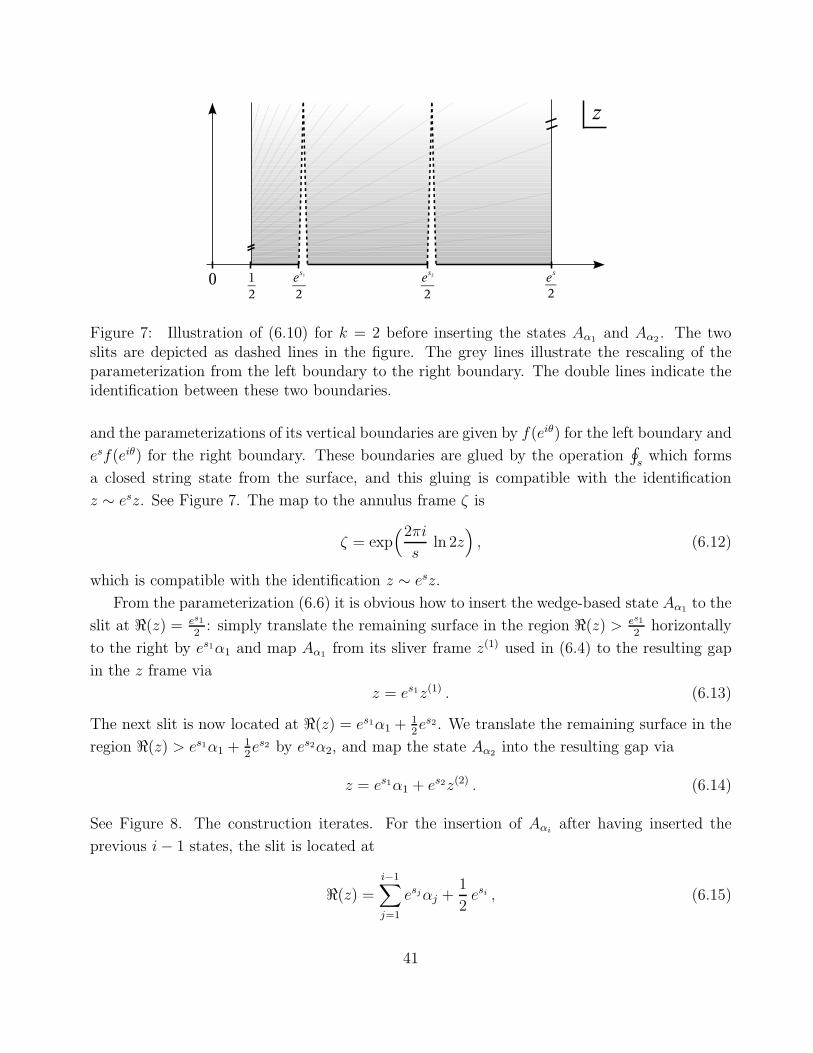
Figure 7: Illustration of (6.10) for k = 2 before inserting the states Aα1 and Aα2 . The twoslits are depicted as dashed lines in the figure. The grey lines illustrate the rescaling of theparameterization from the left boundary to the right boundary. The double lines indicate theidentification between these two boundaries.
and the parameterizations of its vertical boundaries are given by f(eiθ) for the left boundary and
esf(eiθ) for the right boundary. These boundaries are glued by the operation∮
swhich forms
a closed string state from the surface, and this gluing is compatible with the identification
z ∼ esz. See Figure 7. The map to the annulus frame ζ is
ζ = exp(2πi
sln 2z
), (6.12)
which is compatible with the identification z ∼ esz.
From the parameterization (6.6) it is obvious how to insert the wedge-based state Aα1 to the
slit at ℜ(z) = es1
2: simply translate the remaining surface in the region ℜ(z) > es1
2horizontally
to the right by es1α1 and map Aα1 from its sliver frame z(1) used in (6.4) to the resulting gap
in the z frame via
z = es1z(1) . (6.13)
The next slit is now located at ℜ(z) = es1α1 + 12es2. We translate the remaining surface in the
region ℜ(z) > es1α1 + 12es2 by es2α2, and map the state Aα2 into the resulting gap via
z = es1α1 + es2z(2) . (6.14)
See Figure 8. The construction iterates. For the insertion of Aαiafter having inserted the
previous i− 1 states, the slit is located at
ℜ(z) =i−1∑
j=1
esjαj +1
2esi , (6.15)
41

Figure 8: Illustration of (6.10) for k = 2 with gaps of width es1α1 and of width es2α2 insertedat the two slits. Compare this with Figure 7. The states Aα1 and Aα2 are then mapped intothese gaps.
and we translate the remaining surface to the right of the slit by esiαi. Then we map the state
Aαiinto the resulting gap via
z =
i−1∑
j=1
esjαj + esiz(i) . (6.16)
At the end of the process, the whole surface corresponding to (6.10), which we denote by Σ, is
located in the z frame in the region
1
2≤ ℜ(z) ≤
k∑
j=1
esjαj +1
2es . (6.17)
The parameterization of the identified left and right boundaries of this resulting surface Σ are
not related by scaling z ∼ esz , so we cannot map Σ directly to the annulus frame via (6.12).
To restore this relation, we use the prescription given in section 6.1 of [41]. We shift the entire
surface Σ horizontally by
a0 =1
es − 1
k∑
j=1
esjαj . (6.18)
With this value of the shift, Σ is then located in the region
1
2+ a0 ≤ ℜ(z) ≤ es
(1
2+ a0
), (6.19)
and the gluing of the left to the right boundary of Σ is now compatible with the identification
z ∼ esz. This translated frame is called the natural z frame. The total map from the coordinate
z(i) of the wedge surface on which Aαiis defined to the natural z frame is a combination of the
42

map (6.16) and a horizontal translation by a0. It is thus given by
z = ℓi + esiz(i) , (6.20)
where
ℓi =
i−1∑
j=1
αj esj + a0 , ℓ1 = a0 . (6.21)
It is consistent with the identification z ∼ esz in the natural z frame to map Σ to the annulus
frame ζ via (6.12). The gluing to the closed string coordinate patch is unaffected by our manip-
ulations in the z frame, as was shown in [41]. One may worry that the horizontal translations of
the surfaces may have resulted in a relative rotation in the ζ frame. This is not the case, as can
be easily seen from the regularized analysis of [41]. We can thus analytically map the surface
that defines the closed string state (6.10) to an annulus that has exactly the same modulus as
the annulus that defines∮
sP(0, s). In particular, all closed string surface states contributing to
|B∗(Ψ)〉 for wedge-based solutions are represented on exactly the same Riemann surface. This
remarkable property of the Schnabl propagator strip will be crucial for our explicit calculations
in section 7.
The b-ghost line integrals BR(si) in (6.10) have a simple representation in the natural z
frame. Indeed, mapping the line integrals BR(si) from their initial z-frame representation (6.7)
in the presence of slits to their final location in the natural z frame, we find
− BR(si), Aαi → −
∫
C(si)
dz
2πi(z − ℓi)b(z) [. . .] − [. . .]
∫
C(si)
dz
2πi(z − ℓi+1)b(z) . (6.22)
The dots [. . .] in (6.22) represent the operator insertions for Aαi. Note that the difference in
the endpoints of the contour C(si) generated by translation of the contour in the direction of
the real axis vanishes in the Schnabl limit as discussed in [41]. Since both contours in (6.22)
have the same endpoint on the closed string boundary, the contours can be connected. From
the relation ℓi+1 = ℓi + esiαi we find
− BR(si), Aαi →
∮dz
2πi(z − ℓi)b(z) [. . .] + esiαi [. . .]B+
R , (6.23)
where the contour encircles the operators [. . .] counterclockwise and
B+R =
∫ i∞
−i∞
dz
2πib(z) . (6.24)
We do not write the t dependence on the endpoints of the integration contour of B+R because
the integral does not depend on the choice of t. To see this, note that
L+R ≡ Q,B+
R (6.25)
43

generates horizontal translations in the z frame. It was shown in [41] that the closed string
boundary is unaffected by such translations in the Schnabl limit. It follows that the integrand
in (6.24) vanishes along the closed string boundary.16 Thus the operator B+R does not depend
on the choice of t. The position of this insertion is given implicitly by the operator ordering in
the correlator.
We have assembled all the ingredients required to explicitly calculate |B∗(Ψ)〉 with B = B
for wedge-based solutions. In fact, the map from the wedge surfaces on which the solutions are
defined to the natural z frame are explicitly given in (6.20) and the positions and conformal
factors of operator insertions on the surface Σ can be explicitly calculated. The b-ghost line
integrals BR(si) have the simple representation (6.23) in the natural z frame. Finally, the map
from the natural z frame to the annulus frame is explicitly given in (6.12). We conclude that
the boundary state |B∗(Ψ)〉 is explicitly calculable for wedge-based solutions if we use the half-
propagator strips associated with Schnabl’s B. We will now use this knowledge to illustrate
the vanishing of terms with more than one solution insertion in the limit s→ 0.
6.2 The s→ 0 limit revisited
In this subsection we first examine the open-closed vertex encoded in |B(1)∗ (Ψ)〉 constructed
using the Schnabl propagator strip. The open string local coordinate can be calculated explicitly
and one can confirm that this open-closed vertex is not real for finite s. We can also confirm
that the reality condition is recovered in the s→ 0 limit, where the vertex becomes the familiar
singular one used in the definition of W (V,Ψ) discussed in section 5.3. We then consider
|B(k)∗ (Ψ)〉 with k ≥ 2 constructed using the Schnabl propagator strip and argue that they
vanish in the s→ 0 limit.
As explained earlier in (5.11), the geometrical configuration of |B(1)∗ (Ψ)〉 can be reduced to
that of∮
sΨP(0, s). To examine the reality of this vertex, it is sufficient to consider the case
where the open string field is a generic state |φ〉 in the Fock space. Since a state in the Fock
space is a wedge state of unit width with a local operator insertion, the surface associated with
φP(0, s) has total width 12(es +1) in the z frame. The necessary shift a0 for the natural z frame
from the formula (6.18) with k = 1, α1 = 1, and s1 = 0 is
a0 =1
es − 1. (6.26)
For small s, it can be expanded as
a0 ≃1
s− 1
2+ O(s) . (6.27)
16This can also be explicitly confirmed by mapping (6.24) to the annulus frame ζ and evaluating the integrand
at |ζ| = e−π2
s .
44

The position zp of the operator insertion associated with |φ〉 in the natural z frame is
zp = 1 + a0 =es
es − 1, (6.28)
and the local coordinate for the open string is given by
z(ξ) = zp + f(ξ) (6.29)
with f(ξ) defined in (6.2). Since the natural z frame with the identification z ∼ esz is singular
in the limit s→ 0, it is convenient to map this to the annulus ζ frame. We then map it further
to the upper-half plane to compare it with W (V,Ψ). The local coordinate for the open string
in the ζ frame is
ζ(ξ) = exp
[2πi
s( ln 2z(ξ) − ln 2zp )
]= exp
(2πi
sln
[1 +
f(ξ)
1 + a0
] ), (6.30)
where we rotated the ζ frame to satisfy ζ(0) = 1 for convenience. The surface associated with
the state∮
sφP(0, s) in the ζ frame is an annulus with inner radius r = e−
π2
s . We further map
this to the upper-half plane of u by the following conformal transformation:
u = i1 − ζ
1 + ζ. (6.31)
The puncture is located at u = 0 and the outer boundary of unit radius in the ζ frame is
mapped to the real axis. For small s, the inner boundary of the annulus is mapped to a small,
almost circular closed curve around u = i in this frame. The local coordinate now takes the
form
u(ξ) = tan(πs
ln[1 +
f(ξ)
1 + a0
]). (6.32)
When s is small and as θ → π/2, u(eiθ) is a curve that rotates along a small circle around the
point u = i. As discussed in section 5.3, the reality of the open-closed vertex requires u(−ξ) =
−u(ξ). While f(−ξ) = −f(ξ), the coordinate u(ξ) in (6.32) does not satisfy u(−ξ) = −u(ξ).Thus the open-closed vertex is not real for finite s.
Let us now consider the limit s→ 0. We can make use of the expansion
ln[1 +
f
1 + a0
]≃ sf − 1
2s2(f + f 2) + O(s3) , (6.33)
which is valid for any |ξ| ≤ 1 satisfying |ξ − i| > ǫ with fixed ǫ > 0 because |f(ξ)| is bounded
in this region. We then find
u(ξ) = tan(πf − π
2s(f + f 2) + O(s3)
),
= tan(πf) − π
2s(f + f 2) sec2(πf) + O(s3) .
(6.34)
45

The limit s→ 0 is perfectly well defined and we find
lims→0
u(ξ) = tan(πf) = tan(2 arctan(ξ)) =2ξ
1 − ξ2. (6.35)
This result is valid for the region |ξ − i| > ǫ on the unit disk, as stated above. We can see
that (6.35) is, in fact, the local coordinate map (4.34) for the identity state. The closed string
coordinate curve becomes a vanishingly small curve around u = i in this limit, and we have
recovered, as expected, the open-closed vertex used to define the observable W (V,Ψ). In this
limit, of course, the open-closed vertex is real.
Let us now examine the limit s→ 0 of the state |B(k)∗ (Ψ)〉 in (3.20) for arbitrary k. Naively,
one might expect that only the leading term k = 0, the boundary state |B〉, survives in this
limit because the integration region for every Schwinger parameter collapses as s → 0. We
have seen in section 4.4 that this reasoning fails for |B(1)∗ (Ψ)〉. This is the open-closed vertex
examined above. In this case, the integral over s1 covers the entire range of the rotational
modulus of the associated surface even in the limit s → 0. See (4.26). For general choices of
propagator strips, the Schwinger parameters si represent moduli of an annulus with insertions of
the classical solution. The b-ghost line integrals BR(si) provide the measure for this integration
over moduli. For the Schnabl propagator strip and wedge-based solutions, the modulus of the
annulus depends only on s, and the Schwinger parameters si represent position moduli for the
insertions. It is instructive to calculate explicitly the position moduli by examining the maps
of solution insertions to the annulus. We will show that in the limit s → 0, the integration
over all Schwinger parameters s1, . . . , sk only covers a one-dimensional subspace of the position
moduli. We will argue that this is consistent with the vanishing of |B(k)∗ (Ψ)〉 with k ≥ 2 in the
limit s→ 0 for regular solutions.
Consider any point t(i) on the boundary of the wedge surface of width αi for the state Aαi
in (6.10). We have 12≤ t(i) ≤ 1
2+αi. By (6.12) and (6.20), this term is mapped on the annulus
frame to the point
ζi = eiθi with θi =2π
sln 2
[a0 +
i−1∑
j=1
esjαj + esit(i)]. (6.36)
It will be useful to consider the angular separation between a point t(p) on Aαpand a point t(q)
46

on Aαqin the limit s→ 0. We choose q > p for definiteness. Recalling a0 = O(s−1), we obtain
θq − θp =2π
sln
[a0 +
∑q−1j=1 e
sjαj + esqt(q)
a0 +∑p−1
j=1 esjαj + espt(p)
]
=2π
sln
[1 +
1
a0
(t(q) − t(p) +
q−1∑
j=p
αj
)+ O(s2)
]
= 2πt(q) − t(p) +
∑q−1j=p αj
∑kj=1 αj
+ O(s) ,
(6.37)
where we used the explicit expression for a0 from (6.18) in the last step and, since 0 ≤ si ≤ s
for all i, we simply treated all O(si) terms as O(s) terms. We also assumed that the sum of αi’s
in the denominator above is greater than zero. This is clearly satisfied if αi > 0 for all i. We
conclude from (6.37) that the angular separation between t(p) and t(q) on the unit circle |ζ | = 1
freezes up in the limit s → 0: it becomes independent of all Schwinger parameters si. Thus
the relative positions of all points mapped to the open string boundary of the annulus are fixed
in this limit. As the closed string coordinate patch in the annulus frame is also independent
of all si and is only a function of s, the only remaining modulus that can vary as we integrate
over the si is the relative angle of all operator insertions with respect to the closed string
coordinate patch. We conclude that a k dimensional integral over the Schwinger parameters si
is confined to a one-dimensional subspace of moduli in the limit s → 0. As the line integrals
BR(si) supply the correct measure for the k-dimensional integration and the integration region
becomes degenerate, this is consistent with the vanishing of the integrals with k ≥ 2 in the
limit s→ 0.
We can apply this analysis to the state |B(k)∗ (Ψ)〉 with k ≥ 2 for solutions Ψ which are
defined on wedge surfaces of nonvanishing width. Again, as in section 4.4, we assume that the
solution Ψ satisfies some regularity condition that ensures a nonsingular behavior in the limit
s→ 0. Then we conclude from the above argument that all |B(k)∗ (Ψ)〉 with k ≥ 2 vanish in this
limit. This explicit analysis of the si dependence of the maps to the annulus for the Schnabl
gauge propagator thus illustrates the more general argument of section 4.4.
7 The BCFT boundary state from analytic solutions
In this section we explicitly calculate |B∗(Ψ)〉 constructed using the Schnabl propagator strips
for various known wedge-based solutions. We analyze Schnabl’s tachyon vacuum solution and
the two known analytic solutions for marginal deformations with regular operator products.
We find that
|B∗(Ψ)〉 = 0 for all s (7.1)
47

in the case of the tachyon vacuum solution and
|B∗(Ψ)〉 = |B∗〉 for all s (7.2)
with no additional BRST-exact term in the case of marginal deformations.
7.1 Schnabl’s solution for tachyon condensation
Schnabl’s solution ΨS for tachyon condensation is given by [6]
ΨS = limN→∞
[ N∑
n=0
ψ′n − ψN
], ψ′
n ≡ d
dnψn , (7.3)
where
〈φ, ψn−1〉 = −〈 f φ(0) c(1)B+R c(n) 〉Wn
for n > 1 (7.4)
and
〈φ, ψ0〉 ≡ limn→1
〈φ, ψn−1〉 = 〈 f φ(0) c(1) 〉W1 . (7.5)
The goal of this subsection is the calculation of |B∗(ΨS)〉. As a warm-up exercise, it is instructive
to calculate
|B(1)∗ (ψ0)〉 = − e
π2
s(L0+L0)
∮
s
∫ s
0
ds1 P(0, s1) BR(s1), ψ0P(s1, s) . (7.6)
The required shift a0 from (6.18) is given by
a0 =es1
es − 1, (7.7)
and the operator c(1) in (7.5) is mapped to e−s1c(es1 + a0). The operator insertions in the
natural z frame are
− e−s1
∫
C(s1)
dz
2πi(z − a0) b(z) c(e
s1 + a0) − e−s1c(es1 + a0)
∫
C(s1)
dz
2πi(z − a0 − es1) b(z)
= e−s1
∮dz
2πi(z − a0) b(z) c(e
s1 + a0) + c(es1 + a0)B+R
= 1 + c(es1 + a0)B+R = − B+
R c(es1 + a0) ,
(7.8)
where the first line corresponds to (6.22), the second line corresponds to (6.23), and we used the
anticommutation relation B+R, c(t) = −1 in the last step. From the identification z+ = es z−
in the natural z frame, we find
∫dz+2πi
b(z+) = e−s
∫dz−2πi
b(z−) (7.9)
48
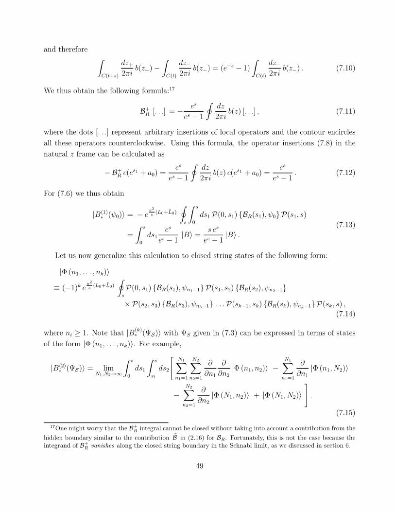
and therefore∫
C(t+s)
dz+2πi
b(z+) −∫
C(t)
dz−2πi
b(z−) = (e−s − 1)
∫
C(t)
dz−2πi
b(z−) . (7.10)
We thus obtain the following formula:17
B+R [. . .] = − es
es − 1
∮dz
2πib(z) [. . .] , (7.11)
where the dots [. . .] represent arbitrary insertions of local operators and the contour encircles
all these operators counterclockwise. Using this formula, the operator insertions (7.8) in the
natural z frame can be calculated as
− B+R c(e
s1 + a0) =es
es − 1
∮dz
2πib(z) c(es1 + a0) =
es
es − 1. (7.12)
For (7.6) we thus obtain
|B(1)∗ (ψ0)〉 = − e
π2
s(L0+L0)
∮
s
∫ s
0
ds1 P(0, s1) BR(s1), ψ0P(s1, s)
=
∫ s
0
ds1es
es − 1|B〉 =
s es
es − 1|B〉 .
(7.13)
Let us now generalize this calculation to closed string states of the following form:
|Φ (n1, . . . , nk)〉
≡ (−1)k eπ2
s(L0+L0)
∮
s
P(0, s1) BR(s1), ψn1−1P(s1, s2) BR(s2), ψn2−1
× P(s2, s3) BR(s3), ψn3−1 . . .P(sk−1, sk) BR(sk), ψnk−1P(sk, s) ,
(7.14)
where ni ≥ 1. Note that |B(k)∗ (ΨS)〉 with ΨS given in (7.3) can be expressed in terms of states
of the form |Φ (n1, . . . , nk)〉. For example,
|B(2)∗ (ΨS)〉 = lim
N1,N2→∞
∫ s
0
ds1
∫ s
s1
ds2
[N1∑
n1=1
N2∑
n2=1
∂
∂n1
∂
∂n2
|Φ (n1, n2)〉 −N1∑
n1=1
∂
∂n1
|Φ (n1, N2)〉
−N2∑
n2=1
∂
∂n2|Φ (N1, n2)〉 + |Φ (N1, N2)〉
].
(7.15)
17One might worry that the B+R
integral cannot be closed without taking into account a contribution from the
hidden boundary similar to the contribution
B in (2.16) for BR. Fortunately, this is not the case because theintegrand of B+
Rvanishes along the closed string boundary in the Schnabl limit, as we discussed in section 6.
49

In the calculation of |Φ (n1, . . . , nk)〉, the operators we insert for ψni−1 in the natural z frame
are
− e−si c(esi + ℓi)B+R c(ni e
si + ℓi) , (7.16)
where
ℓi =i−1∑
j=1
nj esj + a0 , ℓ1 = a0 . (7.17)
All the operators for the state |Φ (n1, . . . , nk)〉 can be written using the formula (6.23) as
k∏
i=1
[− e−si
∮dz
2πi(z − ℓi) b(z) c(e
si + ℓi)B+R c(ni e
si + ℓi) − ni c(esi + ℓi)B+
R c(ni esi + ℓi)B+
R
]
=
k∏
i=1
[− B+
R c(ni esi + ℓi) − ni c(e
si + ℓi)B+R + ni c(e
si + ℓi)B+R
]
=
k∏
i=1
[− B+
R c(ni esi + ℓi)
].
(7.18)
Using the anticommutation relation B+R , c(t) = −1 and (B+
R )2 = 0 repeatedly, we find
B+R c(t1)B+
R c(t2) . . .B+R c(tk) = (−1)k−1 B+
R c(tk) =(−1)k es
es − 1, (7.19)
where we used (7.11) in the last step. Therefore we have
k∏
i=1
[− B+
R c(ni esi + ℓi)
]=
es
es − 1(7.20)
and thus
|Φ (n1, . . . , nk)〉 =es
es − 1|B〉 . (7.21)
Note that this is independent of ni. This means that the ψ′n piece of the solution does not
contribute to |B∗(ΨS)〉 because all derivatives of |Φ (n1, . . . , nk)〉 with respect to ni vanish. In
particular, mixed terms that involve ψ′n and ψN do not contribute to |B∗(ΨS)〉. Therefore the
whole contribution to |B∗(ΨS)〉 comes entirely from the ‘phantom’ term −ψN of the solution,
namely,
|B(k)∗ (ΨS)〉 = (−1)k lim
N1,...,Nk→∞
∫ s
0
ds1
∫ s
s1
ds2 . . .
∫ s
sk−1
dsk |Φ (N1, N2, . . . , Nk)〉. (7.22)
Since |Φ (N1, . . . , Nk)〉 is independent of Ni, the limit N1, . . . , Nk → ∞ is trivial.18 The re-
sult (7.21) is also independent of si. Thus the integrals over si in (7.22) simply gives the
18 In particular, the limit N1, . . . , Nk → ∞ is independent of the order in which we take Ni → ∞.
50

following factor: ∫ s
0
ds1
∫ s
s1
ds2
∫ s
s2
ds3 . . .
∫ s
sk−1
dsk =sk
k!. (7.23)
We therefore conclude that
|B∗(ΨS)〉 =
[1 +
∞∑
k=1
sk
k!(−1)k es
es − 1
]|B〉 =
[1 + (e−s − 1)
es
es − 1
]|B〉 = 0 . (7.24)
In [37, 33] it was shown that the gauge-invariant observables W (V,Ψ) vanish for the tachyon
vacuum solution ΨS . Their result can be reproduced by calculating the on-shell part of the
k = 1 term |B(1)∗ (ΨS)〉 and taking the limit s→ 0. The result (7.24) can thus be viewed as the
generalization of the calculation in [37] to the off-shell part and to finite s. Indeed, the terms
with k ≥ 2 in (7.24) are suppressed for small s, consistent with our analysis in section 6.2. In
the limit s → 0 the k = 1 term by itself cancels the original boundary state |B〉. In summary,
we conclude that |B∗(ΨS)〉 for Schnabl’s tachyon vacuum solution ΨS vanishes for any finite s:
|B∗(ΨS)〉 = 0 for B = B and any finite s. (7.25)
This is consistent with Sen’s conjecture that the D-brane disappears at the tachyon vacuum.
7.2 Factorization of |B∗(Ψ)〉 into matter and ghost sectors
We have seen that |B(k)∗ (ΨS)〉 is proportional to |B〉 for any k. In particular, this means that
the ghost sector of |B(k)∗ (ΨS)〉 is the same as the ghost sector of |B〉, namely, the boundary
state |B(bc)〉 of the bc CFT. This boundary state satisfies the relations
( bn − b−n ) |B(bc)〉 = 0 , ( cn + c−n ) |B(bc)〉 = 0 (7.26)
for all n ∈ Z. If the state |B∗(Ψ)〉 factorizes into matter and ghost sectors as
|B∗(Ψ)〉 = |B(matter)∗ (Ψ)〉 ⊗ |B(bc)〉 , (7.27)
it follows from Q |B∗(Ψ)〉 = 0 and (7.26) that the matter part |B(matter)∗ (Ψ)〉 satisfies the relation
for conformal boundary conditions
(L(matter)n − L
(matter)−n ) |B(matter)
∗ (Ψ)〉 = 0 . (7.28)
While our claim is that the state |B∗(Ψ)〉 coincides with the BCFT boundary state |B∗〉 up to
a possible BRST-exact term, the state |B∗(Ψ)〉 factorized as (7.27) can be a consistent BCFT
boundary state without any BRST-exact term. It is therefore important to examine for what
solutions the ghost part of |B∗(Ψ)〉 becomes the boundary state |B(bc)〉 of the bc CFT.
51

We now claim that the ghost part of a closed string state of the form
eπ2
s(L0+L0)
∮
s
P(0, s1) BR(s1), A1P(s1, s2) BR(s2), A2P(s2, s3) BR(s3), A3 . . .
× P(sk−1, sk) BR(sk), AkP(sk, s)
(7.29)
coincides with the boundary state of the bc CFT if open string fields A1, A2, . . . , Ak of ghost
number one are made of wedge states with
• local operator insertions of the c ghost and its derivatives,
• b-ghost line integrals B+R ,
• arbitrary insertions of matter operators, and
• line integrals L+R = Q,B+
R of the energy-momentum tensor. We demand that there are
no other operators on the contour of each L+R.
This can be shown in the following way. First consider the case where there are no line integrals
of L+R. The b-ghost integral BR(si) in BR(si), Ai can be written in the form (6.23):
BR(si), Aαi → −
∮dz
2πi(z − ℓi) b(z) [. . .] − esiαi [. . .]B+
R , (7.30)
where αi is the length of the wedge state associated with Ai and ℓi is defined in (6.21). Nonva-
nishing contributions to the first term come only from local operator insertions of the c ghost
and its derivatives in [. . .]. Therefore, after performing the integrals of the form (7.30), remain-
ing operator insertions in the ghost sector are insertions of B+R and insertions of the c ghost
and its derivatives. It then follows from (B+R)2 = 0 and the transformation property (7.9) that
there must be at least one insertion of the c ghost or its derivatives between two insertions of
B+R for the result to be nonvanishing. However, since the total ghost number vanishes, there
must be only one insertion of the c ghost or its derivatives between two insertions of B+R . Then
such contributions can be calculated using the formula (7.19). In fact, terms which contain
derivatives of the c ghost vanish because the right-hand side of (7.19) is independent of ti’s.
Nonvanishing contributions are of the form (7.19) and no ghost operators remain in the end.
We have thus shown that the ghost part of (7.29) coincides with |B(bc)〉.Let us next consider the case where there is one line integral of L+
R. The insertion of L+R in
the definition of a state Ai appears in the form
〈φ , Ai〉 = 〈 f φ(0) [. . .]1 L+R [. . .]2〉Wαi
, (7.31)
where we denoted all the operator insertions to the left of the L+R line integral by [. . .]1 and
those to the right by [. . .]2. Such separation is possible because of our assumption that there
52
are no operators on the contour of L+R. The state Ai can be written as
Ai = −∂tAi(t)∣∣∣t=0
, (7.32)
where the state Ai(t) for t > 0 is defined by19
〈φ , Ai(t) 〉 = 〈 f φ(0) [. . .]1 g [. . .]2 〉Wαi+twith g(z) = z + t . (7.33)
Since Ai(t) belongs to the class of states considered before, the ghost part of (7.29) with Ai
replaced by Ai(t) for any positive t coincides with |B(bc)〉. Therefore, the ghost part of (7.29)
with Ai replaced by ∂tAi(t) also coincides with |B(bc)〉. It thus follows that the ghost part
of (7.29) with Ai given by (7.32) also coincides with |B(bc)〉. It is straightforward to generalize
the proof to the case with an arbitrary number of insertions of L+R. We conclude that the state
|B∗(Ψ)〉 takes the form (7.27) if the solution Ψ consists of wedge states with local operator
insertions of the c ghost and its derivatives, line integrals B+R and L+
R, and arbitrary insertions
of matter operators.20
This condition on the solution for which |B∗(Ψ)〉 satisfies (7.27) is a sufficient condition
and is not a necessary condition. However, this class of states covers all known wedge-based
analytic solutions such as Schnabl’s tachyon vacuum solution [6] as analyzed in section 7.1
and the solutions associated with marginal deformations for both regular and singular operator
products constructed in [16, 17, 20, 25].
In the case of marginal deformations with regular operator products, the solutions in Schnabl
gauge constructed in [16, 17] and those in [25] are expected to be gauge-equivalent. We just
argued that these different solutions give the same state |B∗(Ψ)〉 in the form (7.27). We thus
expect that the form (7.27) is preserved for a certain class of gauge transformations. We have
shown in section 3.4 that the state |B∗(Ψ)〉 changes under a gauge transformation δχΨ =
Qχ+ [ Ψ, χ ] by the following BRST-exact term:
δχ|B∗(Ψ)〉 = Q[e
π2
s(L0+L0)
∮
s
∫ s
0
dtP∗(0, t) [BR(t), χ ]P∗(t, s)]. (7.34)
Consider a closed string state of the form
eπ2
s(L0+L0)
∮
s
P(0, s1) BR(s1), A1P(s1, s2) BR(s2), A2P(s2, s3) BR(s3), A3 . . .
× P(si−1, si) [BR(si), Ai ]P(si, si+1) . . .P(sk−1, sk) BR(sk), AkP(sk, s) ,
(7.35)
19 The definition of Ai(t) can be extended to t < 0 until operator insertions in [. . .]1 and g [. . .]2 collide. Thederivative of Ai(t) at t = 0 is therefore well defined.
20 In general, if we have a one-parameter family of closed string states of the form (7.29) with their ghostsectors being |B(bc)〉, ghost sectors of closed string states obtained by taking derivatives with respect to theparameter are also given by |B(bc)〉. We considered the case with line integrals of L+
Ras a particular example of
this generalization because ψ′
n in the tachyon vacuum solution contains a line integral of L+R, but various other
generalizations will be possible. Derivatives of the c ghost can also be treated in this way.
53

where Ai carries ghost number zero and all other states A1, A2, . . . , Ak carry ghost number one.
They are made of wedge states with local operator insertions of the c ghost and its derivatives,
line integrals B+R and L+
R, and arbitrary insertions of matter operators. The b-ghost integral
BR(si) in [BR(si), Ai ] for the Grassmann-even state Ai can be written as
[BR(si), Aαi] → −
∮dz
2πi(z − ℓi) b(z) [. . .] + esiαi [. . .]B+
R , (7.36)
which follows from the same manipulations that led to (6.23) for Grassmann-odd states. Line
integrals of L+R can be treated in the same way as before so that it is sufficient to consider
the case when they are absent. After performing the integrals of the form (7.30) and (7.36),
remaining operator insertions in the ghost sector are again insertions of B+R and insertions of the
c ghost and its derivatives. In this case, however, the total ghost number is −1 and thus we have
one more insertions of B+R than insertions of the c ghost and its derivatives. Any term with more
than one insertion of B+R immediately vanishes because of (B+
R)2 = 0 and the transformation
property (7.9). In the case of one insertion of B+R , we do not have any other insertions of
ghost operators, and it follows from the formula (7.11) that the contribution vanishes. We thus
conclude that δχ|B∗(Ψ)〉 vanishes if the solution Ψ and the gauge parameter χ consist of wedge
states with local operator insertions of the c ghost and its derivatives, line integrals B+R and L+
R,
and arbitrary insertions of matter operators. In particular, gauge transformations generated
by gauge parameters made of wedge states with only matter operator insertions do not change
the state |B∗(Ψ)〉.
7.3 Marginal deformations with regular operator products
Deformations of BCFT generated by a matter primary field V of weight one are exactly marginal
when operator products V (t1)V (t2) . . . V (tn) are regular. In this case we expect to have a one-
parameter family of solutions to the equation of motion of open string field theory. Analytic
solutions for such marginal deformations with regular operator products were constructed in [16,
17, 25]. In [37, 36], the gauge-invariant observables W (V,Ψ) were calculated for these solutions,
and the results confirmed the relation (1.2). These calculations essentially extracted the on-
shell part of |B(1)∗ (Ψ)〉 in the limit s → 0. In this section we calculate the full state |B∗(Ψ)〉
constructed using the Schnabl propagator strips for these analytic solutions to see if it coincides
with the BCFT boundary state
|B∗〉 = exp
[λ
∫ 2π
0
dθ V (θ)
]|B〉 , (7.37)
where θ with 0 ≤ θ ≤ 2π parameterizes the boundary of the disk.
54

7.3.1 The leading term
The leading term Ψ(1) defined by
〈φ,Ψ(1) 〉 = 〈 f φ(0) cV (1) 〉W1 (7.38)
is identical for all solutions [16, 17, 25] associated with a marginal operator V . Let us calculate
|B(1)∗ (Ψ(1))〉 = − e
π2
s(L0+L0)
∮
s
∫ s
0
ds1 P(0, s1) BR(s1),Ψ(1)P(s1, s) . (7.39)
The required shift a0 from (6.18) is given by
a0 =es1
es − 1. (7.40)
Using (6.23), the operator insertions in the natural z frame are∮
dz
2πi(z − a0) b(z) cV (es1 + a0) + es1 cV (es1 + a0)B+
R
= es1 V (es1 + a0) + es1 cV (es1 + a0)B+R
= −es1 B+R cV (es1 + a0) .
(7.41)
The ghost sector of these operator insertions is identical to the one calculated in (7.12) for the
tachyon vacuum solution. We obtain
− es1 B+R cV (es1 + a0) =
es es1
es − 1V (es1 + a0) . (7.42)
If we define
u1 = es1 + a0 =es es1
es − 1, (7.43)
we observe that ∫ s
0
ds1es es1
es − 1V (es1 + a0) =
∫ e2s
es−1
es
es−1
du1 V (u1) . (7.44)
Namely, the measure factor∂u1
∂s1=
es es1
es − 1(7.45)
has been correctly provided through the calculation. Since the point es
es−1and the point e2s
es−1
are identified in the natural z frame, the operator corresponds to∫ 2π
0
dθ V (θ) (7.46)
in the ζ frame, where θ parameterizes the boundary |ζ | = 1 as ζ = eiθ. Therefore we find
|B(1)∗ (Ψ(1))〉 = − e
π2
s(L0+L0)
∮
s
∫ s
0
ds1 P(0, s1) BR(s1),Ψ(1)P(s1, s) =
∫ 2π
0
dθ V (θ) |B〉 .(7.47)
This is indeed the O(λ) term in the path-ordered exponential (7.37) that we expected.
55

7.3.2 Regular marginal deformations in Schnabl gauge
Let us next calculate |B∗(Ψ)〉 with Ψ being the Schnabl-gauge solutions for marginal deforma-
tions constructed in [16, 17]. The solution Ψ is given by
Ψ =∞∑
n=1
λn Ψ(n) , (7.48)
where21
〈φ,Ψ(n) 〉 = −∫ 1
0
dt1
∫ 1
0
dt2 . . .
∫ 1
0
dtn−1 〈 f φ(0) cV (1)
× V (1 + t1)V (1 + t1 + t2) . . . V (1 + t1 + t2 + . . .+ tn−2)
× B+R cV (1 + t1 + t2 + . . .+ tn−1) 〉W1+t1+t2+...+tn−1
.
(7.49)
The calculation of the ghost sector has been done in section 7.1 so that we only need to calculate
the matter sector.22
There are two terms which contribute to |B∗(Ψ)〉 at O(λ2). The first one is
|B(2)∗ (Ψ(1))〉 = e
π2
s(L0+L0)
∮
s
∫ s
0
ds1
∫ s
s1
ds2 P(0, s1) BR(s1),Ψ(1)
× P(s1, s2) BR(s2),Ψ(1)P(s1, s) .
(7.50)
The operator insertion in the natural z frame is given by
es
es − 1
∫ s
0
ds1
∫ s
s1
ds2 es1 V
( eses1 + es2
es − 1
)es2 V
( eses1 + eses2
es − 1
), (7.51)
where we used (7.20) to calculate the ghost sector. The second one is
|B(1)∗ (Ψ(2))〉 = − e
π2
s(L0+L0)
∮
s
∫ s
0
ds1 P(0, s1) BR(s1),Ψ(2)P(s1, s) . (7.52)
The operator insertion in the natural z frame is given by
es
es − 1
∫ s
0
ds1
∫ 1
0
dt1 es1 V
( eses1 + t1 es1
es − 1
)es1 V
( eses1 + es t1 es1
es − 1
). (7.53)
If we define
s′1 = s1 , s′2 = s1 + ln t1 , (7.54)
21 Note that the operator B in [17] corresponds to −B+R
in this paper. This expression can be derived from (3.3)of [17] by replacing B with −B+
Rand by using B+
R, c(t) = −1 and (B+
R)2 = 0 recursively.
22 The separation of matter and ghost sectors depends on a frame. We separate them in the sliver frame usedin (7.49). For example, the operator cV in the sliver frame z(i) is divided into e−sic and esiV in the natural zframe via the conformal transformation (6.20).
56

this can be written as follows:
es
es − 1
∫ s
0
ds′1
∫ s′1
−∞
ds′2 es′1 V
( eses′1 + es′2
es − 1
)es′2 V
( eses′1 + eses′2
es − 1
). (7.55)
Note that the second factor of es1 in (7.53) has been changed to es′2 because of the Jacobian
∂(s′1, s′2)
∂(s1, t1)=
1
t1. (7.56)
The two expressions (7.51) and (7.55) are combined to give
es
es − 1
∫ s
0
ds1
∫ s
−∞
ds2 es1 V
( eses1 + es2
es − 1
)es2 V
( eses1 + eses2
es − 1
). (7.57)
If we define
u1 =eses1 + es2
es − 1, u2 =
eses1 + eses2
es − 1, (7.58)
this expression can be written in the following form:∫
Γ(2)′du1du2 V (u1)V (u2) , (7.59)
where we have used∂(u1, u2)
∂(s1, s2)=
es
es − 1es1 es2 . (7.60)
Since
es1 = u1 − e−su2 , es2 = u2 − u1 , (7.61)
the integration region Γ(2)′ can be characterized by
1 ≤ u1 − e−su2 ≤ es , 0 ≤ u2 − u1 ≤ es . (7.62)
Using the identification z ∼ esz in the natural z frame, this integral can also be written as∫
Γ(2)
du1du2 V (u1)V (u2) (7.63)
with Γ(2) given by
1 ≤ esu1 − u2 ≤ es , 0 ≤ u2 − u1 ≤ 1 . (7.64)
It is straightforward to generalize the calculations to the case of O(λn). The details are
presented in appendix A.1. The matter sector of the boundary state |B∗(Ψ)〉 can be written in
the z frame with the identification z ∼ esz as follows:
∞∑
n=0
λn
∫
Γ(n)
du1du2 . . . dun V (u1)V (u2) . . . V (un) , (7.65)
57

where the region Γ(n) is given by
0 ≤ u2 − u1 ≤ 1 , 0 ≤ u3 − u2 ≤ 1 , . . . 0 ≤ un − un−1 ≤ 1 , 1 ≤ esu1 − un ≤ es . (7.66)
In appendix A.2 we use the identification z ∼ esz in the z frame repeatedly to show that
∫
Γ(n)
du1du2 . . dun V (u1)V (u2) . . V (un) =
∫ es
1
du1
∫ es
u1
du2 . .
∫ es
un−1
dun V (u1)V (u2) . . V (un) .
(7.67)
It follows that
∞∑
n=0
λn
∫
Γ(n)
du1du2 . . . dun V (u1)V (u2) . . . V (un) = exp
[λ
∫ es
1
du V (u)
]. (7.68)
Therefore we conclude that
|B∗(Ψ)〉 = exp
[λ
∫ 2π
0
dθ V (θ)
]|B〉 . (7.69)
7.3.3 Other solutions for regular marginal deformations
We have so far considered solutions in Schnabl gauge, and thus the choice of the propagator
strip B = B and the gauge condition on the solution BΨ = 0 are correlated. However, neither
the explicit calculability of |B∗(Ψ)〉 nor the factorizability (7.27) depends on the Schnabl-gauge
condition BΨ = 0. We next consider the analytic solutions for regular marginal deformations
constructed in [25], which do not satisfy BΨ = 0. While there is an obstruction in the construc-
tion of solutions in Schnabl gauge for marginal deformations with singular operator products,
the solutions in [25] can be generalized to such singular cases and they still belong to the class
of solutions discussed in section 7.2.
The solution ΨL constructed in [25] is given by
ΨL =
∞∑
n=1
Ψ(n)L , (7.70)
where
〈φ ,Ψ(n)L 〉 = λn
∫ 2
1
dt2
∫ 3
t2
dt3
∫ 4
t3
dt4 . . .
∫ n
tn−1
dtn 〈 f φ(0) cV (1)V (t2)V (t3) . . . V (tn) 〉Wn.
(7.71)
While ΨL solves the equation of motion, it does not satisfy the reality condition
Ψ = hc−1(Ψ⋆) (7.72)
58

on the string field, where hc denotes hermitian conjugation. A real solution Ψreal that satis-
fies (7.72) was constructed from ΨL using a gauge transformation [25]. As the gauge parameter
χ of the required gauge transformation is of the type described in section 7.2,23 we conclude
from the discussion in that section that
|B∗(ΨL)〉 = |B∗(Ψreal)〉 . (7.73)
It is thus sufficient to calculate |B∗(ΨL)〉.Consider the term with k insertions Ψ
(n1)L , . . . ,Ψ
(nk)L in |B∗(ΨL)〉:
(−1)k eπ2
s(L0+L0)
∮
s
∫ s
0
ds1
∫ s
s1
ds2 . . .
∫ s
sk−1
dsk P(0, s1) BR(s1),Ψ(n1)L
× P(s1, s2) BR(s2),Ψ(n2)L P(s2, s3) BR(s3),Ψ
(n3)L . . .
×P(sk−1, sk) BR(sk),Ψ(nk)L P(sk, s) .
(7.74)
At O(λn), all partitions ~n = n1, . . . , nk with
k∑
i=1
ni = n (7.75)
contribute. The solution ΨL has the structure discussed in section 7.2 and we can thus eliminate
all ghost-sector operators in the natural z frame as described in that section. We show in
appendix B.1 that the numerical factor which remains after this manipulation is given by
∆k
k∏
i=1
esi with ∆k = 1 +1
es − 1− 1
es − 1
k∏
i=1
(1 − ni) . (7.76)
Let us denote the marginal operators from the insertion Ψ(ni)L in the natural z-frame pic-
ture as V (t(i)1 ), V (t
(i)2 ), . . . , V (t
(i)ni ) with t
(i)1 ≤ t
(i)2 ≤ . . . ≤ t
(i)ni . Note that cV (t
(i)1 ) is the only
unintegrated vertex operator from Ψ(ni)L and the others V (t
(i)2 ), . . . , V (t
(i)ni ) are integrated ver-
tex operators. After the calculation of the ghost sector in the natural z frame, we expect the
factor (7.76) to provide the correct measure for the integration over positions of the operators
V (t(i)1 ) with i = 1 . . . k. This is indeed the case:
∂(t(1)1 , t
(2)1 , . . . , t
(k)1 )
∂(s1, s2, . . . , sk)= ∆k
k∏
i=1
esi , (7.77)
as we show in appendix B.2.
23 The infinitesimal gauge parameter χ for this transformation is proportional to ln√U with the state U
defined in [25]. As U is a wedge-based state with only matter operator insertions and U = 1 + O(λ), weconclude that χ is well defined perturbatively in λ and of the form described in section 7.2.
59

The operator insertions in the natural z frame of any term (7.74) with partition ~n thus take
the form ∫
Γ(~n)
dt(1)1 dt
(1)2 . . . dt
(k)nk−1dt
(k)nk
V (t(1)1 )V (t
(1)2 ) . . . V (t
(k)nk−1)V (t(k)
nk) (7.78)
for some integration region Γ(~n) associated with the particular partition ~n. The integration
regions are complicated, and we were not able to explicitly combine the regions Γ(~n) of all
partitions into the expected form. We instead choose a different approach to show that the
BCFT boundary state is indeed recovered. Consider any point in the integration region Γ(~n) of
any partition ~n which contributes to |B∗(Ψ)〉 at O(λn). The associated positions t(1)1 , . . . , t(k)nk
in the z frame are mapped to a set of angles θ1, . . . , θn on the unit circle in the ζ frame:
t(1)1 , . . . , t(k)nk → eiθ1 , . . . , eiθn with 0 ≤ θ1 ≤ · · · ≤ θq ≤ · · · ≤ θn ≤ 2π . (7.79)
Note that this is a map between sets, and the order of insertion points t(i)j in the z-frame will
in general be a cyclic permutation of the ordering of the angles θq. In particular, we do not
expect that t(1)1 is necessarily mapped to θ1.
We pick any one of the angles in the set θ1, . . . , θn, and denote its index by q. We now
vary this angle, keeping all other angles fixed to their original values. In appendix B.3 we show
that for any θq−1 ≤ θ ≤ θq+1, we can find a partition ~n such that some point in its integration
region Γ(~n) maps to the positions
eiθ1 , . . . , eiθq−1, eiθ, eiθq+1 , . . . , eiθn (7.80)
in the ζ frame. As θ is varied, one generically reaches the boundary of the integration region
Γ(~n) of the current partition ~n. We show that such points can always be smoothly matched to
the boundary of the integration region Γ(~n) of a different partition ~n. The variation of θ can
thus continue until it either coincides with θq−1 or θq+1.24 Denoting the image of the region
Γ(~n) in the ζ frame by ζ(Γ(~n)
), we conclude that
eiθ1, . . . , eiθq−1 , eiθ, eiθq+1, . . . , eiθn ⊂⋃
~n
ζ(Γ(~n)
)for all θq−1 ≤ θ ≤ θq+1 . (7.81)
Note that the angles θq with q 6= q are not arbitrary because they are determined by the point in
the integration ~n that we picked originally as the starting point for the argument. It is obvious,
however, that we can use the above argument iteratively for all 1 ≤ q ≤ n and complete the
integration region to all θ1, . . . , θn satisfying
0 ≤ θ1 ≤ . . . ≤ θn ≤ 2π . (7.82)
24 For the special case of q = 1, the lower boundary of the variation is θ1 = 0. Similarly, the upper boundaryof the variation for q = n is θn = 2π.
60

This is the integration region expected from (7.37) at O(λn). As the above argument requires
a choice of a starting point, it does not rule out multiple covering and we conclude that
|B∗(ΨL)〉 =
∞∑
n=0
Cn
n!
[λ
∫ 2π
0
dθ V (θ)
]n
|B〉 for some Cn ∈ N . (7.83)
It now remains to show that Cn = 1 for all n. Consider any partition ~n = n1, . . . , nkwith k ≥ 2. In the natural z frame, the last operator insertion of Ψ(n1) and the first operator
insertion of Ψ(n2) are located at
t(1)n1≤ es1n1 + a0 , t
(2)1 = es1n1 + es2 + a0 (7.84)
with
a0 =1
es − 1
k∑
i=1
ni esi ≤ esn
es − 1. (7.85)
In the ζ frame, their angular separation ∆θ is thus bounded from below:
∆θ ≥ ∆θmin with ∆θmin =2π
slog
[esn+ (es − 1)(n1 + 1)
esn+ (es − 1)n1
]. (7.86)
The lower bound ∆θmin > 0 is independent of the Schwinger parameters si. Using cyclicity, we
similarly conclude that
∆θ ≤ 2π − ∆θmin . (7.87)
Now consider the subset of the integration region (7.82) where all operator insertions are sep-
arated by less than the angle ∆θmin, namely,
|θi − θj | < ∆θmin for all 1 ≤ i, j ≤ n . (7.88)
This is a finite region for finite s which can only be covered by ζ(Γ(~n)
)with the partition
~n = n of k = 1. On the other hand, we have shown in (4.26) that the region from
|B(1)∗ (Ψ
(n)L )〉 covers the rotational modulus exactly once, so the subset (7.88) of the integra-
tion region is covered precisely once. Therefore, there cannot be multiple coverings of the
integration region (7.82) and we obtain
Cn = 1 for all n . (7.89)
Recalling the relation (7.73), we conclude that
|B∗(ΨL)〉 = |B∗(Ψreal)〉 = exp
[λ
∫ 2π
0
dθ V (θ)
]|B〉 . (7.90)
61

8 Discussion
In this paper we have constructed a class of BRST-invariant closed string states |B∗(Ψ)〉 for
any open string field solution Ψ. The construction depends on a choice of a propagator strip.
Modifying the propagator strip or performing a gauge transformation on the classical solution
generically changes |B∗(Ψ)〉 by a BRST-exact term. We calculated |B∗(Ψ)〉 for various known
analytic solutions choosing the Schnabl propagator strip and found that |B∗(Ψ)〉 precisely
coincides with the BCFT boundary state |B∗〉 of the background that the solutions are expected
to describe. This is the first construction of the full BCFT boundary state from solutions of
open string field theory.
While we claim that the state |B∗(Ψ)〉 in general coincides with the BCFT boundary state
|B∗〉 up to a possible BRST-exact term, such a term can be absent if the state |B∗(Ψ)〉 factorizes
into the matter and ghost sectors as (7.27). We presented a sufficient condition on the solution
Ψ such that |B∗(Ψ)〉, constructed with the choice of the Schnabl propagator strip, factorizes
in this way. It would be useful to understand better when the factorization (7.27) holds. Our
analysis indicates that the remarkable simplifications associated with the choice of Schnabl
propagator strip play an important role for the factorization (7.27). It follows from the analysis
in [41] that all Riemann surfaces associated with closed string states of the form∮
sΣ(0, s)
coincide in the Schnabl limit when Ai in the definition (2.23) of Σ(0, s) are wedge-based states.
In fact, the resulting Riemann surface is an annulus whose modulus only depends on s. This
outstanding feature was crucially important in this paper. We expect from the analysis in [13]
that the simplifications associated with Schnabl’s propagator carry over into other projector-
based propagators.
Because the boundary state is a basic object in BCFT, we believe that our construction of
|B∗〉 from a solution Ψ provides an important step towards establishing the map from classi-
cal solutions of open string field theory to BCFT’s. Partial success in the reverse map from
BCFT’s to classical solutions was achieved in [20, 25, 27] for backgrounds connected by arbi-
trary marginal deformations. A systematic procedure to construct solutions from the BCFT
operator that implements a change of boundary conditions along a segment on the boundary
was presented for the bosonic string in [25] and for the superstring in [27]. Our ambitious goal
is a complete understanding of the relation between BCFT’s and classical solutions of open
sting field theory.
The construction of the closed string state |B∗(Ψ)〉 is based on the representation (3.4)
of the original BCFT boundary state |B〉 in terms of the half-propagator strip P(0, s). The
state |B∗(Ψ)〉 is obtained by replacing P(0, s) in (3.4) with the half-propagator strip P∗(0, s)
associated with the background Ψ. This construction of |B∗(Ψ)〉 is the primary reason for our
claim that the state |B∗(Ψ)〉 coincides with the BCFT boundary state |B∗〉 up to a possible
62

BRST-exact term, but we have not provided a proof for this claim. We have in addition
examined two lines of argumentation. The first one is based on the limit s → 0 discussed in
section 4.4. Since |B∗(Ψ)〉 changes only by a BRST-exact term as we vary the parameter s,
our claim follows if the relation (4.32) holds and if the claim (1.2) discussed in [37] is proven.
The second argument is that our claim is a consequence of the expected, but not yet proven,
background independence of a version of open-closed string field theory. We may obtain new
insights from further efforts towards a rigorous proof for the claim.
It would be interesting to study the generalization of our construction to open superstring
field theory in the WZW formulation by Berkovits [65, 66]. We can construct BRST-invariant
closed string states in the superstring by replacing Ψ in |B∗(Ψ)〉 with e−ΦQeΦ, where Φ is the
open superstring field and Q is the BRST operator in the superstring. We expect that the
resulting states |B∗(e−ΦQeΦ)〉 are related to the BCFT boundary state. It would be interesting
to study such closed string states extending the discussion in [37] on gauge-invariant observ-
ables [67] for the superstring. The construction of the BCFT boundary state in the superstring
from open superstring fields can then be used for consistency checks on solutions of open su-
perstring field theory. For example, a solution for the tachyon vacuum in this theory has been
proposed in [35], and it would be useful to examine if the state |B∗(e−ΦQeΦ)〉 vanishes for this
solution.
We hope that our construction of |B∗(Ψ)〉 will pave the way to the study of closed string
physics within string field theory. It may lead us to a novel formulation of open-closed string
field theory, and the set of open-closed vertices encoded in |B∗(Ψ)〉 is the first step in this
direction. If we choose a propagator strip associated with a non-BPZ-even gauge condition, we
obtain complex open-closed vertices. To obtain real vertices suitable for open-closed string field
theory, it may be useful to examine if our construction can be generalized to the full propagator
surface of regular linear b-gauges [42].
Since gravity is contained in the closed string sector, a consistent coupling of open strings
to an off-shell closed string in the framework of string field theory can be thought of as a
string theory generalization of the energy-momentum tensor. Apart from the reality issue we
mentioned earlier, the state |B∗(Ψ)〉 can thus be regarded as giving such a generalized energy-
momentum tensor. Its expression in terms of the path-ordered exponential (3.14) is reminiscent
of the energy-momentum tensor of noncommutative gauge theory in terms of open Wilson lines
derived in [68]. While the on-shell part of |B∗(Ψ)〉 is gauge-invariant, the off-shell part is not.
We believe that information contained in its off-shell part, especially when |B∗(Ψ)〉 coincides
with the BCFT boundary state |B∗〉, is useful in understanding the map from solutions to
BCFT’s, but it is an important open problem whether physical observables are contained in
the off-shell part in the context of string theory or of string field theory. For example, off-
shell information in the BCFT boundary state was used in the study of the rolling tachyon by
63

Sen [48]. Finally, the coupling of open string fields to closed string modes plays an important
role in the AdS/CFT correspondence. The study of open string field theory with such open-
closed vertices reviewed in section 5 indicates that a large amount of the closed string physics
can in principle be reproduced, and the results in this paper further provide a prospect that they
might actually be calculable. We hope that exciting developments await us in this direction.
Acknowledgements
We would like to thank Kentaro Hori, Taichiro Kugo, and Hiroshi Kunitomo for useful dis-
cussions. We also thank Ian Ellwood, Leonardo Rastelli, Martin Schnabl, and Ashoke Sen for
discussions and for their valuable comments on an earlier version of the manuscript. M.K.
would like to thank the members of the University of Tokyo at the IPMU and at Komaba for
stimulating discussions and hospitality during this work. Y.O. acknowledges the kind hospital-
ity of the IPMU at the University of Tokyo during part of this work. The work of M.K. was
supported in part by the World Premier International Research Center Initiative of MEXT,
Japan. The work of M.K. and B.Z. is supported by the U.S. DOE grant DE-FG02-05ER41360.
The work of Y.O. is supported in part by Grant-in-Aid for Scientific Research [No. 20340048
(B)] from the Ministry of Education, Science and Culture of Japan.
A Marginal deformations in Schnabl gauge
A.1 The matter sector to all orders
In this appendix we derive (7.65). We generalize the calculations in the subsection to the
following case:
(−1)keπ2
s(L0+L0)
∮
s
∫ s
0
ds1
∫ s
s1
ds2 . . .
∫ s
sk−1
dsk P(0, s1) BR(s1),Ψ(n1)
× P(s1, s2) BR(s2),Ψ(n2)P(s2, s3) BR(s3),Ψ
(n3) . . .× P(sk−1, sk) BR(sk),Ψ
(nk)P(sk, s) ,
(A.1)
wherek∑
i=1
ni = n . (A.2)
64

The operator insertion in the natural z frame is given by
es
es − 1
∫ s
0
ds1
∫ s
s1
ds2 . . .
∫ s
sk−1
dsk
k∏
i=1
[ ∫ 1
0
dt(i)1
∫ 1
0
dt(i)2 . . .
∫ 1
0
dt(i)ni−1 (esi)ni
]
×n∏
a=1
V( eses′1 + . . .+ eses′a + es′a+1 + . . .+ es′n
es − 1
),
(A.3)
where
s′a = si + ln t(i)j−1 with t
(i)0 = 1 (A.4)
for
a = n1 + n2 + . . .+ ni−1 + j , with j = 1, 2, . . . , ni . (A.5)
The integral can be written in terms of s′a as follows:
es
es − 1
∫
Γ(n1,n2,...,nk)
ds′1ds′2 . . . ds
′n
n∏
a=1
es′a V( eses′1 + . . .+ eses′a + es′a+1 + . . .+ es′n
es − 1
), (A.6)
where
∫
Γ(n1,n2,...,nk)
ds′1ds′2 . . . ds
′n =
k∏
i=1
∫ s
s′di−1+1
ds′di+1
∫ s′di+1
−∞
ds′di+2
∫ s′di+1
−∞
ds′di+3 . . .
∫ s′di+1
−∞
ds′di+ni
(A.7)
with
d1 = 0 , di =
i−1∑
j=1
nj for i > 1 , s′d0+1 = 0 . (A.8)
For example, when (n1, n2, n3) = (3, 2, 1), we have
∫
Γ(3,2,1)
ds′1ds′2 . . . ds
′6 =
∫ s
0
ds′1
∫ s′1
−∞
ds′2
∫ s′1
−∞
ds′3
∫ s
s′1
ds′4
∫ s′4
−∞
ds′5
∫ s
s′4
ds′6 . (A.9)
Note that Γ(n1, n2, . . . , nk) satisfies the following relation:∫
Γ(n1,n2,...,nk)
ds′1ds′2 . . . ds
′n
∫ s
−∞
ds′n+1
∫
Γ(n1,n2,...,nk)
ds′1ds′2 . . . ds
′n
∫ s′bk+1
−∞
ds′n+1 +
∫
Γ(n1,n2,...,nk)
ds′1ds′2 . . . ds
′n
∫ s
s′bk+1
ds′n+1
=
∫
Γ(n1,n2,...,nk−1,nk+1)
ds′1ds′2 . . . ds
′n+1 +
∫
Γ(n1,n2,...,nk,1)
ds′1ds′2 . . . ds
′n+1 .
(A.10)
Using this relation recursively, the integration regions from all partitions are combined to give
∑
n1+n2+...+nk=n
∫
Γ(n1,n2,...,nk)
ds′1ds′2 . . . ds
′n =
∫ s
0
ds′1
∫ s
−∞
ds′2
∫ s
−∞
ds′3 . . .
∫ s
−∞
ds′n . (A.11)
65

If we define
ua =eses′1 + . . .+ eses′a + es′a+1 + . . .+ es′n
es − 1for 1 ≤ a ≤ n , (A.12)
the contributions from all partitions can be written in the following form:
es
es − 1
∫ s
0
ds′1
∫ s
−∞
ds′2
∫ s
−∞
ds′3 . . .
∫ s
−∞
ds′n
n∏
a=1
es′a V( eses′1 + . . .+ eses′a + es′a+1 + . . .+ es′n
es − 1
)
=
∫
Γ(n)′du1du2 . . . dun V (u1)V (u2) . . . V (un) .
(A.13)
To see this, note that
∂(u1, u2, . . . , un)
∂(s′1, s′2, . . . , s
′n)
=1
(es − 1)n
n∏
a=1
es′a
∣∣∣∣∣∣∣∣∣∣∣∣∣
es 1 1 . . . 1 1es es 1 . . . 1 1es es es . . . 1 1...
......
. . ....
...es es es . . . es 1es es es . . . es es
∣∣∣∣∣∣∣∣∣∣∣∣∣
=es(es − 1)n−1
(es − 1)n
n∏
a=1
es′a =es
es − 1
n∏
a=1
es′a .
(A.14)
Since
es′1 = u1 − e−sun , es′2 = u2 − u1 , es′3 = u3 − u2 , . . . es′n = un − un−1 , (A.15)
the integration region Γ(n)′ can be characterized by
1 ≤ u1 − e−sun ≤ es , 0 ≤ u2 − u1 ≤ es , 0 ≤ u3 − u2 ≤ es , . . . 0 ≤ un − un−1 ≤ es .
(A.16)
Using the identification z ∼ esz in the natural z frame, this integral can also be written as
∫
Γ(n)
du1du2 . . . dun V (u1)V (u2) . . . V (un) (A.17)
with Γ(n) given by
1 ≤ esu1 − un ≤ es , 0 ≤ u2 − u1 ≤ 1 , 0 ≤ u3 − u2 ≤ 1 , . . . 0 ≤ un − un−1 ≤ 1 . (A.18)
This completes the derivation of (7.65).
66

A.2 Recovering the BCFT boundary state
The matter sector of the boundary state |B∗(Ψ)〉 with Ψ being solutions for marginal deforma-
tions can be written in the z frame with the identification z ∼ esz as follows:
∞∑
n=0
λn
∫
Γ(n)
du1du2 . . . dun V (u1)V (u2) . . . V (un) , (A.19)
with Γ(n) given in (A.18). In this appendix we show that
∫
Γ(n)
du1du2 . . dun V (u1)V (u2) . . V (un) =
∫ es
1
du1
∫ es
u1
du2 . .
∫ es
un−1
dun V (u1)V (u2) . . V (un) .
(A.20)
Let us first consider the case with n = 2. We define a region U (2) in the (u1, u2) plane by
U (2) ≡
(u1, u2)∣∣ u1 ≤ u2 , u2 ≤ esu1
. (A.21)
The region Γ(2) is the subset of U (2) given by
Γ(2) ≡
(u1, u2)∣∣ 0 ≤ u2 − u1 ≤ 1 , 1 ≤ esu1 − u2 ≤ es
. (A.22)
If we define Γ(a1, a2) ⊂ U (2) by
Γ(a1, a2) ≡
(u1, u2)∣∣ 0 ≤ u2 − u1 ≤ a1 , 0 ≤ esu1 − u2 ≤ a2
, (A.23)
the region Γ(2) can be written as
Γ(2) = Γ(1, es) − Γ(1, 1) . (A.24)
Consider the map g : U (2) → U (2) given by
g((u1, u2)
)= (u2, e
su1) . (A.25)
Note that the set of angles θ1, θ2 in the ζ frame that the points (u1, u2) are mapped to
via (6.12) is invariant under g. The region Γ(a1, a2) is mapped under g as
Γ(a1, a2)g−→ Γ(a2, e
sa1) . (A.26)
Thus the region Γ(2) is mapped by a sequence of maps g as follows:
Γ(2) = Γ(1, es) − Γ(1, 1)g−→ Γ(es, es) − Γ(1, es)
g−→ Γ(es, e2s) − Γ(es, es)g−→ Γ(e2s, e2s) − Γ(es, e2s)
g−→ . . . .(A.27)
The map g is invertible and its inverse is given by
g−1((u1, u2)
)= (e−su2, u1) . (A.28)
67

Under g−1, the region Γ(a1, a2) is mapped as
Γ(a1, a2)g−1
−→ Γ(e−sa2, a1) . (A.29)
Thus the region Γ(2) is mapped by a sequence of maps g−1 as follows:
Γ(2) = Γ(1, es) − Γ(1, 1)g−1
−→ Γ(1, 1) − Γ(e−s, 1)
g−1
−→ Γ(e−s, 1) − Γ(e−s, e−s)g−1
−→ Γ(e−s, e−s) − Γ(e−2s, e−s)g−1
−→ . . . .(A.30)
Therefore, any point (u1, u2) ∈ U (2) can be mapped to Γ(2) either by a sequence of the map g
or by a sequence of the map g−1. Let us denote this map by G. This map
G : U (2) → Γ(2) (A.31)
is uniquely defined because the images of Γ(2) under different sequences of either g or g−1
do not intersect. Furthermore, G is onto because it is the identity map when restricted to
(u1, u2) ∈ Γ(2).
The region Γ(2) for the path-ordered exponential in (A.20) at O(λ2) is the subset of U (2)
given by
Γ(2) ≡
(u1, u2)∣∣ 1 ≤ u1 ≤ u2 ≤ es
. (A.32)
If we define Γ(ui ≤ a) ⊂ U (2) by
Γ(ui ≤ a) ≡
(u1, u2)∣∣ u1 ≤ u2 , u2 ≤ esu1 , ui ≤ a
, (A.33)
the region Γ(2) can be written as
Γ(2) = Γ(u2 ≤ es) − Γ(u1 ≤ 1) . (A.34)
Under the map g, the region Γ(ui ≤ a) is mapped as
Γ(u1 ≤ a)g−→ Γ(u2 ≤ esa) , Γ(u2 ≤ a)
g−→ Γ(u1 ≤ a) . (A.35)
Thus the region Γ(2) is mapped by a sequence of maps g as follows:
Γ(2) = Γ(u2 ≤ es) − Γ(u1 ≤ 1)g−→ Γ(u1 ≤ es) − Γ(u2 ≤ es)
g−→ Γ(u2 ≤ e2s) − Γ(u1 ≤ es)g−→ Γ(u1 ≤ e2s) − Γ(u2 ≤ e2s)
g−→ . . . .(A.36)
Under the inverse map g−1, the region Γ(ui ≤ a) is mapped as
Γ(u1 ≤ a)g−1
−→ Γ(u2 ≤ a) , Γ(u2 ≤ a)g−1
−→ Γ(u1 ≤ e−sa) . (A.37)
68

Thus the region Γ(2) is mapped by a sequence of maps g−1 as follows:
Γ(2) = Γ(u2 ≤ es) − Γ(u1 ≤ 1)g−1
−→ Γ(u1 ≤ 1) − Γ(u2 ≤ 1)
g−1
−→ Γ(u2 ≤ 1) − Γ(u1 ≤ e−s)g−1
−→ Γ(u1 ≤ e−s) − Γ(u2 ≤ e−s)g−1
−→ . . . .(A.38)
Therefore, any point (u1, u2) ∈ U (2) can be mapped to Γ(2) either by a sequence of maps g
or by a sequence of maps g−1. Let us denote this map by G. This map
G : U (2) → Γ(2) (A.39)
is uniquely defined because the images of Γ(2) under different sequences of either g or g−1
do not intersect. Furthermore, G is onto because it is the identity map when restricted to
(u1, u2) ∈ Γ(2).
We have thus constructed a map G : U (2) → Γ(2) and a map G : U (2) → Γ(2). Both maps
are onto. We now define a map H : Γ(2) → Γ(2) that is the restriction of G to (u1, u2) ∈ Γ(2):
H = G∣∣∣
eΓ(2). (A.40)
Similarly, we define H : Γ(2) → Γ(2) as the restriction of G to (u1, u2) ∈ Γ(2):
H = G∣∣∣Γ(2)
. (A.41)
The composition of these two maps, H H , is the identity map on Γ(2). To show this, assume
the contrary, i.e., assume (u′1, u′2) 6= (u1, u2) with
(u′1, u′2) = H H
((u1, u2)
). (A.42)
As H H is built from sequences of g and g−1, the points (u1, u2) ∈ Γ(2) and (u′1, u′2) ∈ Γ(2) are
related by some sequence of maps g or g−1. However, since
g . . . g︸ ︷︷ ︸i−times
(Γ(2)
)∩ Γ(2) = ∅ for i 6= 0 ,
g−1 . . . g−1
︸ ︷︷ ︸j−times
(Γ(2)
)∩ Γ(2) = ∅ for j 6= 0 ,
(A.43)
we conclude that they cannot be related by a nontrivial sequence and thus
(u′1, u′2) = (u1, u2) , (A.44)
in contradiction with the assumption. Thus H H is indeed the identity map on Γ(2). Similarly,
one can show that H H is the identity map on Γ(2). The maps H and H are therefore inverses
69

of each other, and in particular they must be one-to-one and onto. We have thus constructed
a map between the integration region Γ(2) and the integration region Γ(2),
H : Γ(2) → Γ(2) , one-to-one and onto . (A.45)
Note that for each fixed (u1, u2) this map is either a finite25 sequence of maps g or a finite
sequence of maps g−1. Furthermore, recall that the set of angles θ1, θ2 in the ζ frame that
the points (u1, u2) map to, is invariant under the maps g and g−1. We can thus decompose Γ(2)
appropriately and map each piece of the region to reconstruct Γ(2). We can explicitly perform
this procedure for a given finite s. We thus conclude that the integration regions Γ(2) and Γ(2)
are identical:∫
Γ(2)
du1du2 V (u1)V (u2) =
∫
eΓ(2)
du1du2 V (u1)V (u2) . (A.46)
This proves (A.20) for n = 2.
This proof can be easily generalized to arbitrary n > 2. We define a region U (n) by
U (n) ≡
(u1, u2, . . . , un)∣∣ u1 ≤ u2 , u2 ≤ u3 , . . . , un−1 ≤ un , un ≤ esu1
. (A.47)
The region Γ(n) is the subset of U (n) given by
Γ(n) =
(u1, u2, . . . , un)∣∣ 0 ≤ u2−u1 ≤ 1 , 0 ≤ u3−u2 ≤ 1 , . . . , 1 ≤ esu1−un ≤ es
. (A.48)
If we define Γ(a1, a2, . . . , an) ⊂ U (n) by
Γ(a1, a2, . . . , an) ≡
(u1, u2, . . . , un)∣∣ 0 ≤ u2 − u1 ≤ a1 , 0 ≤ u3 − u2 ≤ a2 , . . . ,
0 ≤ un − un−1 ≤ an−1 , 0 ≤ esu1 − un ≤ an
,
(A.49)
the region Γ(n) can be written as
Γ(n) = Γ(1, 1, . . . , 1, es) − Γ(1, 1, . . . , 1) . (A.50)
Consider the map g : U (n) → U (n) given by
g((u1, u2, . . . , un)
)= (u2, u3, . . . , un, e
su1) . (A.51)
Note that the set of angles θ1, θ2, . . . , θn in the ζ frame that the points (u1, u2, . . . , un) are
mapped to via (6.12) is invariant under g. The region Γ(a1, a2, . . . , an) is mapped under g as
Γ(a1, a2, . . . , an)g−→ Γ(a2, a3, . . . , an, e
sa1) . (A.52)
25The maps g and g−1 have a fixed-point at the origin in the (u1, u2) plane. However, as neither Γ(2) nor Γ(2)
contains the origin, the map H is perfectly well defined and unaffected by this singularity.
70
Thus the region Γ(n) is mapped by a sequence of maps g as follows:
Γ(n) = Γ(1, 1, . . . , 1, es) − Γ(1, 1, . . . , 1)g−→ Γ(1, 1, . . . , 1, es, es) − Γ(1, 1, . . . , 1, es)g−→ Γ(1, 1, . . . , 1, es, es, es) − Γ(1, 1, . . . , 1, es, es)
g−→ . . . .
(A.53)
The map g is invertible and its inverse is given by
g−1((u1, u2, . . . , un)
)= (e−sun, u1, u2, . . . , un−1) . (A.54)
Under g−1, the region Γ(a1, a2, . . . , an) is mapped as
Γ(a1, a2, . . . , an)g−1
−→ Γ(e−san, a1, a2, . . . , an−1) . (A.55)
Thus the region Γ(n) is mapped by a sequence of maps g−1 as follows:
Γ(n) = Γ(1, 1, . . . , 1, es) − Γ(1, 1, . . . , 1)
g−1
−→ Γ(1, 1, . . . , 1) − Γ(e−s, 1, 1, . . . , 1)
g−1
−→ Γ(e−s, 1, 1, . . . , 1) − Γ(e−s, e−s, 1, 1, . . . , 1)g−1
−→ . . . .
(A.56)
Therefore, any point (u1, u2, . . . , un) ∈ U (n) can be mapped to Γ(n) either by a sequence of the
map g or by a sequence of the map g−1. Let us denote this map by G. This map
G : U (n) → Γ(n) (A.57)
is uniquely defined because the images of Γ(n) under different sequences of either g or g−1
do not intersect. Furthermore, G is onto because it is the identity map when restricted to
(u1, u2, . . . , un) ∈ Γ(n).
The region Γ(n) for the path-ordered exponential at O(λn) is the subset of U (n) given by
Γ(n) ≡
(u1, u2, . . . , un)∣∣ 1 ≤ u1 ≤ u2 ≤ . . . ≤ un ≤ es
. (A.58)
If we define Γ(ui ≤ a) ⊂ U (n) by
Γ(ui ≤ a) ≡
(u1, u2, . . . , un)∣∣ u1 ≤ u2 , u2 ≤ u3 , . . . , un−1 ≤ un , un ≤ esu1 , ui ≤ a
,
(A.59)
the region Γ(n) can be written as
Γ(n) = Γ(un ≤ es) − Γ(u1 ≤ 1) . (A.60)
Under the map g, the region Γ(ui ≤ a) is mapped as
Γ(u1 ≤ a)g−→ Γ(un ≤ esa) ,
Γ(u2 ≤ a)g−→ Γ(u1 ≤ a) , Γ(u3 ≤ a)
g−→ Γ(u2 ≤ a) , . . . Γ(un ≤ a)g−→ Γ(un−1 ≤ a) .
(A.61)
71

Thus the region Γ(n) is mapped by a sequence of maps g as follows:
Γ(n) = Γ(un ≤ es) − Γ(u1 ≤ 1)g−→ Γ(un−1 ≤ es) − Γ(un ≤ es)
g−→ Γ(un−2 ≤ es) − Γ(un−1 ≤ es)g−→ . . .
g−→ Γ(u1 ≤ es) − Γ(u2 ≤ es)g−→ Γ(un ≤ e2s) − Γ(u1 ≤ es)
g−→Γ(un−1 ≤ e2s) − Γ(un ≤ e2s)g−→ . . .
.
(A.62)
Under the inverse map g−1, the region Γ(ui ≤ a) is mapped as
Γ(u1 ≤ a)g−1
−→ Γ(u2 ≤ a) , Γ(u2 ≤ a)g−1
−→ Γ(u3 ≤ a) , . . . Γ(un−1 ≤ a)g−1
−→ Γ(un ≤ a) ,
Γ(un ≤ a)g−1
−→ Γ(u1 ≤ e−sa) .
(A.63)
Thus the region Γ(n) is mapped by a sequence of maps g−1 as follows:
Γ(n) = Γ(un ≤ es) − Γ(u1 ≤ 1)g−1
−→ Γ(u1 ≤ 1) − Γ(u2 ≤ 1)
g−1
−→ Γ(u2 ≤ 1) − Γ(u3 ≤ 1)g−1
−→ . . .
g−1
−→ Γ(un−1 ≤ 1) − Γ(un ≤ 1)g−1
−→ Γ(un ≤ 1) − Γ(u1 ≤ e−s)
g−1
−→ Γ(u1 ≤ e−s) − Γ(u2 ≤ e−s)g−1
−→ . . . .
(A.64)
Therefore, any point (u1, u2, . . . , un) ∈ U (n) can be mapped to Γ(n) either by a sequence of maps
g or by a sequence of maps g−1. Let us denote this map by G. This map
G : U (n) → Γ(n) (A.65)
is uniquely defined because the images of Γ(n) under different sequences of either g or g−1
do not intersect. Furthermore, G is onto because it is the identity map when restricted to
(u1, u2, . . . , un) ∈ Γ(n).
We have thus constructed a map G : U (n) → Γ(n) and a map G : U (n) → Γ(n). Both maps
are onto. We now define a map H : Γ(n) → Γ(n) that is the restriction of G to (u1, u2, . . . , un) ∈Γ(n):
H = G∣∣∣
eΓ(n). (A.66)
Similarly, we define H : Γ(n) → Γ(n) as the restriction of G to (u1, u2, . . . , un) ∈ Γ(n):
H = G∣∣∣Γ(n)
. (A.67)
72
The composition of these two maps, H H , is the identity map on Γ(n). To show this, assume
the contrary, i.e., assume (u′1, u′2, . . . , u
′n) 6= (u1, u2, . . . , un) with
(u′1, u′2, . . . , u
′n) = H H
((u1, u2, . . . , un)
). (A.68)
As HH is built from sequences of g and g−1, the points (u1, u2, . . . , un) ∈ Γ(n) and (u′1, u′2, . . . , u
′n) ∈
Γ(n) are related by some sequence of maps g or g−1. However, since
g . . . g︸ ︷︷ ︸i−times
(Γ(n)
)∩ Γ(n) = ∅ for i 6= 0 ,
g−1 . . . g−1
︸ ︷︷ ︸j−times
(Γ(n)
)∩ Γ(n) = ∅ for j 6= 0 ,
(A.69)
we conclude that they cannot be related by a nontrivial sequence and thus
(u′1, u′2, . . . , u
′n) = (u1, u2, . . . , un) , (A.70)
in contradiction with the assumption. Thus H H is indeed the identity map on Γ(n). Similarly,
one can show that H H is the identity map on Γ(n). The maps H and H are therefore inverses
of each other, and in particular they must be one-to-one and onto. We have thus constructed
a map between the integration region Γ(n) and the integration region Γ(n),
H : Γ(n) → Γ(n) , one-to-one and onto . (A.71)
Note that for each fixed (u1, u2, . . . , un) this map is either a finite sequence of maps g or a finite
sequence of maps g−1. Furthermore, recall that the set of angles θ1, θ2, . . . , θn in the ζ frame
that the points (u1, u2, . . . , un) map to, is invariant under the maps g and g−1. We can thus
decompose Γ(n) appropriately and map each piece of the region to reconstruct Γ(n). We can
explicitly perform this procedure for a given finite s. We thus conclude that the integration
regions Γ(n) and Γ(n) are identical:
∫
Γ(n)
du1du2 . . . dun V (u1)V (u2) . . . V (un) =
∫
eΓ(n)
du1du2 . . . dun V (u1)V (u2) . . . V (un) .
(A.72)
This completes our proof of the claim (A.20).
B The solution ΨL
B.1 Ghost sector
Let us consider the ghost sector of |B(k)∗ (ΨL)〉 in the natural z frame. The value of a0 is
a0 =1
es − 1
k∑
i=1
ni esi . (B.1)
73

The ghost sector of the term (7.74) in the natural z frame can be written as
k∏
i=1
[−
∫
C(si)
dz
2πi(z − ℓi) b(z) c(e
si + ℓi) − c(esi + ℓi)
∫
C(si)
dz
2πi(z − ℓi+1) b(z)
], (B.2)
where
ℓi =i−1∑
j=1
nj esj + a0 , ℓ1 = a0 . (B.3)
This can be calculated as
k∏
i=1
[−
∫
C(si)
dz
2πi(z − ℓi) b(z) c(e
si + ℓi) − c(esi + ℓi)
∫
C(si)
dz
2πi(z − ℓi+1) b(z)
]
=
k∏
i=1
[ ∮dz
2πi(z − ℓi) b(z) c(e
si + ℓi) + ni esi c(esi + ℓi)B+
R
]
=
k∏
i=1
esi
[1 + ni c(e
si + ℓi)B+R
].
(B.4)
Using the same manipulations as in (7.19) we find
c(t1)B+R c(t2)B+
R . . . c(tm)B+R = (−1)m−1 c(t1)B+
R =(−1)m−1
es − 1. (B.5)
Therefore, we havek∏
i=1
esi
[1 + ni c(e
si + ℓi)B+R
]= ∆k
k∏
i=1
esi (B.6)
with
∆k = 1 +1
es − 1− 1
es − 1
k∏
i=1
(1 − ni) . (B.7)
B.2 Measure
In this appendix we calculate the Jacobian
∂(t(1)1 , t
(2)1 , . . . , t
(k)1 )
∂(s1, s2, . . . , sk), (B.8)
where
t(i)1 =
i−1∑
j=1
nj esj + esi + a0 (B.9)
74

with a0 given in (B.1). The derivative of a0 with respect to sj is given by
∂a0
∂sj
=nj
es − 1esj = bj e
sj , (B.10)
where
bj ≡nj
es − 1. (B.11)
We define ∆k by
∂(t(1)1 , t
(2)1 , . . . , t
(k)1 )
∂(s1, s2, . . . , sk)= ∆k
k∏
i=1
esi . (B.12)
It follows from
∂t(i)1
∂sj
=
(nj + bj) esj for j < i ,
(1 + bj) esj for j = i ,
bj esj for j > i
(B.13)
that
∆k =
∣∣∣∣∣∣∣∣∣∣∣∣∣
1 + b1 b2 b3 . . . bk−1 bkn1 + b1 1 + b2 b3 . . . bk−1 bkn1 + b1 n2 + b2 1 + b3 . . . bk−1 bk
......
.... . .
......
n1 + b1 n2 + b2 n3 + b3 . . . 1 + bk−1 bkn1 + b1 n2 + b2 n3 + b3 . . . nk−1 + bk−1 1 + bk
∣∣∣∣∣∣∣∣∣∣∣∣∣
. (B.14)
Let us prove that
∆k = ∆k = 1 +1
es − 1− 1
es − 1
k∏
i=1
(1 − ni) . (B.15)
For k = 1, we have
∆1 = 1 + b1 = 1 +n1
es − 1= ∆1 . (B.16)
For k > 1, we find that
∆k =
∣∣∣∣∣∣∣∣∣
1 + b1 . . . bk−1 0...
. . ....
...n1 + b1 . . . 1 + bk−1 0n1 + b1 . . . nk−1 + bk−1 1
∣∣∣∣∣∣∣∣∣
+ bk
∣∣∣∣∣∣∣∣∣
1 + b1 . . . bk−1 1...
. . ....
...n1 + b1 . . . 1 + bk−1 1n1 + b1 . . . nk−1 + bk−1 1
∣∣∣∣∣∣∣∣∣
. (B.17)
75

The first term on the right-hand side is ∆k−1. The determinant in the second term can be
calculated as follows:∣∣∣∣∣∣∣∣∣∣∣∣∣
1 + b1 b2 b3 . . . bk−1 1n1 + b1 1 + b2 b3 . . . bk−1 1n1 + b1 n2 + b2 1 + b3 . . . bk−1 1
......
.... . .
......
n1 + b1 n2 + b2 n3 + b3 . . . 1 + bk−1 1n1 + b1 n2 + b2 n3 + b3 . . . nk−1 + bk−1 1
∣∣∣∣∣∣∣∣∣∣∣∣∣
=
∣∣∣∣∣∣∣∣∣∣∣∣∣
1 − n1 −n2 −n3 . . . −nk−1 00 1 − n2 −n3 . . . −nk−1 00 0 1 − n3 . . . −nk−1 0...
......
. . ....
...0 0 0 . . . 1 − nk−1 0
n1 + b1 n2 + b2 n3 + b3 . . . nk−1 + bk−1 1
∣∣∣∣∣∣∣∣∣∣∣∣∣
=k−1∏
i=1
(1 − ni) .
(B.18)
We therefore have
∆k = ∆k−1 + bk
k−1∏
i=1
(1 − ni) = ∆k−1 +nk
es − 1
k−1∏
i=1
(1 − ni) . (B.19)
On the other hand, it is easy to see that
∆k − ∆k−1 =nk
es − 1
k−1∏
i=1
(1 − ni) (B.20)
for k > 1. We thus conclude that
∆k = ∆k . (B.21)
B.3 Proof of (7.81)
In this appendix we prove the claim (7.81). We consider an arbitrary point t(1)1 , . . . , t(k)nk in
the integration region Γ(~n) of a partition ~n = (n1, . . . , nk) contributing to |B∗(ΨL)〉 at O(λn).
The insertion points t(1)1 , . . . , t(k)nk in the z frame are mapped to the unit circle in the ζ frame
as
t(1)1 , . . . , t(k)nk → eiθ1 , . . . , eiθq−1 , eiθq , eiθq+1, . . . , eiθn . (B.22)
We will show that for any
θq−1 ≤ θ ≤ θq+1 , (B.23)
we can find a partition ~n such that a point in its integration region Γ(~n) is mapped to the
positions
eiθ1 , . . . , eiθq−1 , eiθ, eiθq+1, . . . , eiθn (B.24)
76

in the ζ frame. We will prove this claim by showing that we can determine the required partition
~n starting from the original partition ~n as we continuously vary θ away from θq. For the following
analysis it is convenient to recall that the integration region of an arbitrary partition ~n. The
position of the first V insertion associated with Ψ(ni) in the natural z frame is given by
t(i)1 =
i−1∑
j=1
nj esj + esi + a0 , (B.25)
while the integration region for the remaining ni−1 insertions, which we will denote as internal
insertions in the following, are given by
t(i)j−1 ≤ t
(i)j ≤ t
(i)1 + esj (j − 1) for j ≥ 2 . (B.26)
Let us denote the insertion position in the original partition ~n which is mapped to the angle θq
by t(i)j . We need to distinguish several cases.
V (t(i)j ) is an internal insertion (j ≥ 2)
Consider first a variation which decreases θ, i.e., θ ≤ θq. If θq−1 = θq then we are already at the
lower end of the interval (B.23) and we are done. If θq−1 < θq then t(i)j > t
(i)j−1, so the internal
insertion is not yet at the lower boundary of its integration region (B.26). Varying t(i)j does
not affect any other positions, so we conclude that we can find a configuration within the exact
same partition ~n for any
θq−1 ≤ θ ≤ θq . (B.27)
Eventually, the internal insertion V (t(i)j ) collides with the previous insertion V (t
(i)j−1), which is
precisely one of the boundaries in the interval (B.23) that we expected to find.
Now consider increasing θ into the range θ > θq. When increasing θ by increasing t(i)j ,
eventually two things can happen: if j < ni and t(i)j+1 ≤ t
(i)1 + esi(j − 1), it follows from (B.26)
that V (t(i)j ) can collide with the next V insertion at t
(i)j+1 which corresponds to the upper
boundary of the interval (B.23) and we are done. Otherwise, t(i)j eventually hits its upper
limit of integration at t(i)j = t
(i)1 + esi(j − 1). Within this partition ~n, the integration region
stops although we have not encountered an operator collision. So this integration region must
smoothly match with another integration region in a different partition ~n. This is indeed the
case. Intuitively, this can be understood as a “breaking” of the solution insertion Ψ(ni) into two
pieces when t(i)j becomes too large. We now have two solution insertions, Ψ(j−1) and Ψ(ni−j+1),
with a new half-propagator strip opening up between them. The relevant partition is thus
obtained by replacing
· · · P(si−1, si)Ψ(ni)P(si, si+1) · · · → · · · P(si−1, si)Ψ
(j−1)P(si, s)Ψ(ni−j+1)P(s, si+1) · · · .
(B.28)
77

We thus have
~n = . . . , ni−1, ni, ni+1, . . . → ~n = . . . , ni−1, (j − 1), (ni−1 − j + 1), ni+1, . . . . (B.29)
It is easy to see that for t(i)j = t
(i)1 + esi(j − 1) in the first partition, the operator insertions
match smoothly to s = si in the second partition. The boundary of the integration region Γ(~n)
at t(i)j = t
(i)1 + esi(j− 1) thus matches smoothly to the boundary of the integration region Γ(~n).
In the new partition ~n, the V insertion at angle θ originates from the first V insertion in the
solution Ψ(ni−j+1). To see that we can then still continue varying θ, we turn to the second case.
V (t(i)j ) is the first insertion in a solution (j = 1)
The insertion position t(i)1 is not independently integrated over in our parameterization using
integrals over si. In fact, to move t(i)1 while keeping all positions fixed, we generically need to
vary all the sm. Recalling (B.13), we find
∂sm
∂t(i)1
> 0 for all 1 ≤ m, i ≤ k . (B.30)
Furthermore, we note that the integral regions (B.26) of internal insertions depend on the sm.
As we vary θ and thus t(i)1 , the following things can happen.
• V (t(i)1 ) can collide with V (t
(i)2 )
This can happen if ni ≥ 2 and constitutes the upper boundary of the interval (B.23).
• An internal insertions hits the upper boundary of its integration
As mentioned above, this is caused by the change in integration regions for internal
insertions as we vary t(i)1 . We have encountered such a situation before in the previous
subsection. Denote the position of the insertion which reaches its upper limit of integration
by t(m)j with j ≥ 2. Just as above we can match this configuration smoothly by breaking
the affected solution into two pieces:
P(sm−1, sm)Ψ(nm)P(sm, sm+1) → P(sm−1, sm)Ψ(j−1)P(sm, s)Ψ(nm−j+1)P(s, sm+1) .
(B.31)
This corresponds to the change of partition
~n = . . . , nm−1, nm, nm+1, . . . → ~n = . . . , nm−1, (j−1), (nm−j+1), nm+1, . . . . (B.32)
For t(m)j = t
(m)1 + esm(j− 1) in the partition ~n, the operator insertions match smoothly to
s = sm in the partition ~n.
78

• sm → sm+1 for some 1 ≤ m < k
This is in a sense the opposite case to the ones we have encountered so far. Instead of
breaking solutions, in this case solutions merge. We match smoothly to a new configura-
tion
. . .P(sm−1, sm)Ψ(nm)P(sm, sm+1)Ψ(nm+1) . . . → . . .P(sm−1, sm+1)Ψ
(nm+nm+1) . . . .
(B.33)
This corresponds to the change of partition
~n = . . . , nm−1, nm, nm+1, nm+2, . . . → ~n = . . . , nm−1, (nm +nm+1), nm+2, . . . . (B.34)
Thus there is no longer an integral over sm present – instead the solution insertion
Ψ(nm+nm+1) carries one more internal integral than the previous solution insertions Ψ(m)
and Ψ(nm+1) combined. Note that if m + 1 = i, then the insertion V (t(i)1 ) which we are
varying corresponds to an internal insertion in the new partition ~n and we have to keep
track of the variation of its position as we did in the previous subsection. If not, we
continue the analysis of this subsection with the new partition ~n.
• sk → s
As we increase θ and thus increase t(i)1 , sk also increases because
∂sk
∂t(i)1
> 0 . (B.35)
Thus eventually we can hit its upper limit of integration sk = s, and the last half-
propagator P(sk, s) in the partition (7.74) collapses. As we generically do not have an
operator collision in this configuration, we need to match it smoothly to a different par-
tition. But in fact, using the cyclic property of∮
s, we can rewrite this configuration
as
[. . . ]
∮
s
P(0, s1) . . .P(sk−1, sk)Ψ(nk)P(sk, s)
∣∣∣∣sk=s
→ [. . . ]
∮
s
P(0, s0)Ψ(nk)P(s0, s1) . . .P(sk−1, s)
∣∣∣∣s0=0
.
(B.36)
After cyclic index relabeling i→ i+1, we again obtain a partition of the form (7.74) with
s1 = 0. This corresponds to the change of partition
~n = n1, . . . , nk−1, nk → ~n = nk, n1, . . . , nk−1 . (B.37)
We can now continue to increase θ, which is now represented by the position t(i+1)1 in ~n.
As we increase θ, the new Schwinger parameter s1 leaves its lower boundary s1 = 0 and
79

enters its allowed region s1 > 0, because
∂s1
∂t(i+1)1
> 0 . (B.38)
• s1 → 0
We can hit s1 = 0 when decreasing θ. This is reversed situation of the collision sk → s
and can be dealt with in the exact same way.
We conclude that we can continue to vary θ throughout the interval (B.23) while keeping all
other insertion angles fixed. This completes the proof of (7.81).
References
[1] E. Witten, “Noncommutative Geometry And String Field Theory,” Nucl. Phys. B 268,
253 (1986).
[2] W. Taylor and B. Zwiebach, “D-branes, tachyons, and string field theory,”
arXiv:hep-th/0311017.
[3] L. Rastelli, “String field theory,” arXiv:hep-th/0509129.
[4] W. Taylor, “String field theory,” arXiv:hep-th/0605202.
[5] E. Fuchs and M. Kroyter, “Analytical Solutions of Open String Field Theory,”
arXiv:0807.4722 [hep-th].
[6] M. Schnabl, “Analytic solution for tachyon condensation in open string field theory,” Adv.
Theor. Math. Phys. 10, 433 (2006) [arXiv:hep-th/0511286].
[7] Y. Okawa, “Comments on Schnabl’s analytic solution for tachyon condensation in Witten’s
open string field theory,” JHEP 0604, 055 (2006) [arXiv:hep-th/0603159].
[8] E. Fuchs and M. Kroyter, “On the validity of the solution of string field theory,” JHEP
0605, 006 (2006) [arXiv:hep-th/0603195].
[9] E. Fuchs and M. Kroyter, “Schnabl’s L0 operator in the continuous basis,” JHEP 0610,
067 (2006) [arXiv:hep-th/0605254].
[10] L. Rastelli and B. Zwiebach, “Solving open string field theory with special projectors,”
arXiv:hep-th/0606131.
80

[11] I. Ellwood and M. Schnabl, “Proof of vanishing cohomology at the tachyon vacuum,”
JHEP 0702, 096 (2007) [arXiv:hep-th/0606142].
[12] E. Fuchs and M. Kroyter, “Universal regularization for string field theory,” JHEP 0702,
038 (2007) [arXiv:hep-th/0610298].
[13] Y. Okawa, L. Rastelli and B. Zwiebach, “Analytic solutions for tachyon condensation with
general projectors,” arXiv:hep-th/0611110.
[14] T. Erler, “Split string formalism and the closed string vacuum,” JHEP 0705, 083 (2007)
[arXiv:hep-th/0611200].
[15] T. Erler, “Split string formalism and the closed string vacuum. II,” JHEP 0705, 084 (2007)
[arXiv:hep-th/0612050].
[16] M. Schnabl, “Comments on marginal deformations in open string field theory,”
arXiv:hep-th/0701248.
[17] M. Kiermaier, Y. Okawa, L. Rastelli and B. Zwiebach, “Analytic solutions for marginal
deformations in open string field theory,” arXiv:hep-th/0701249.
[18] T. Erler, “Marginal Solutions for the Superstring,” JHEP 0707, 050 (2007)
[arXiv:0704.0930 [hep-th]].
[19] Y. Okawa, “Analytic solutions for marginal deformations in open superstring field theory,”
JHEP 0709, 084 (2007) [arXiv:0704.0936 [hep-th]].
[20] E. Fuchs, M. Kroyter and R. Potting, “Marginal deformations in string field theory,” JHEP
0709, 101 (2007) [arXiv:0704.2222 [hep-th]].
[21] Y. Okawa, “Real analytic solutions for marginal deformations in open superstring field
theory,” JHEP 0709, 082 (2007) [arXiv:0704.3612 [hep-th]].
[22] I. Ellwood, “Rolling to the tachyon vacuum in string field theory,” arXiv:0705.0013 [hep-
th].
[23] I. Kishimoto and Y. Michishita, “Comments on Solutions for Nonsingular Currents in Open
String Field Theories,” Prog. Theor. Phys. 118, 347 (2007) [arXiv:0706.0409 [hep-th]].
[24] E. Fuchs and M. Kroyter, “Marginal deformation for the photon in superstring field the-
ory,” arXiv:0706.0717 [hep-th].
81

[25] M. Kiermaier and Y. Okawa, “Exact marginality in open string field theory: a general
framework,” arXiv:0707.4472 [hep-th].
[26] T. Erler, “Tachyon Vacuum in Cubic Superstring Field Theory,” arXiv:0707.4591 [hep-th].
[27] M. Kiermaier and Y. Okawa, “General marginal deformations in open superstring field
theory,” arXiv:0708.3394 [hep-th].
[28] O. K. Kwon, B. H. Lee, C. Park and S. J. Sin, “Fluctuations around the Tachyon Vacuum
in Open String Field Theory,” arXiv:0709.2888 [hep-th].
[29] B. H. Lee, C. Park and D. D. Tolla, “Marginal Deformations as Lower Dimensional D-brane
Solutions in Open String Field theory,” arXiv:0710.1342 [hep-th].
[30] T. Takahashi, “Level truncation analysis of exact solutions in open string field theory,”
JHEP 0801, 001 (2008) [arXiv:0710.5358 [hep-th]].
[31] O. K. Kwon, “Marginally Deformed Rolling Tachyon around the Tachyon Vacuum in Open
String Field Theory,” arXiv:0801.0573 [hep-th].
[32] S. Hellerman and M. Schnabl, “Light-like tachyon condensation in Open String Field The-
ory,” arXiv:0803.1184 [hep-th].
[33] T. Kawano, I. Kishimoto and T. Takahashi, “Gauge Invariant Overlaps for Classical So-
lutions in Open String Field Theory,” arXiv:0804.1541 [hep-th].
[34] T. Kawano, I. Kishimoto and T. Takahashi, “Schnabl’s Solution and Boundary States in
Open String Field Theory,” arXiv:0804.4414 [hep-th].
[35] E. Fuchs and M. Kroyter, “On the classical equivalence of superstring field theories,”
arXiv:0805.4386 [hep-th].
[36] I. Kishimoto, “Comments on gauge invariant overlaps for marginal solutions in open string
field theory,” arXiv:0808.0355 [hep-th].
[37] I. Ellwood, “The closed string tadpole in open string field theory,” arXiv:0804.1131 [hep-
th].
[38] A. Hashimoto and N. Itzhaki, “Observables of string field theory,” JHEP 0201, 028 (2002)
[arXiv:hep-th/0111092].
[39] D. Gaiotto, L. Rastelli, A. Sen and B. Zwiebach, “Ghost structure and closed strings in vac-
uum string field theory,” Adv. Theor. Math. Phys. 6, 403 (2003) [arXiv:hep-th/0111129].
82

[40] L. Rastelli and B. Zwiebach, “The off-shell Veneziano amplitude in Schnabl gauge,”
arXiv:0708.2591 [hep-th].
[41] M. Kiermaier and B. Zwiebach, “One-Loop Riemann Surfaces in Schnabl Gauge,”
arXiv:0805.3701 [hep-th].
[42] M. Kiermaier, A. Sen and B. Zwiebach, “Linear b-Gauges for Open String Fields,”
arXiv:0712.0627 [hep-th].
[43] H. Fuji, S. Nakayama and H. Suzuki, “Open string amplitudes in various gauges,” JHEP
0701, 011 (2007) [arXiv:hep-th/0609047].
[44] M. Asano and M. Kato, “New covariant gauges in string field theory,” Prog. Theor. Phys.
117, 569 (2007) [arXiv:hep-th/0611189].
[45] M. Asano and M. Kato, “General Linear Gauges and Amplitudes in Open String Field
Theory,” arXiv:0807.5010 [hep-th].
[46] L. Rastelli and B. Zwiebach, “Tachyon potentials, star products and universality,” JHEP
0109, 038 (2001) [arXiv:hep-th/0006240].
[47] M. Schnabl, “Wedge states in string field theory,” JHEP 0301, 004 (2003)
[arXiv:hep-th/0201095].
[48] A. Sen, “Rolling tachyon,” JHEP 0204, 048 (2002) [arXiv:hep-th/0203211].
[49] A. Sen, “Tachyon matter,” JHEP 0207, 065 (2002) [arXiv:hep-th/0203265].
[50] A. Sen, “Time evolution in open string theory,” JHEP 0210, 003 (2002)
[arXiv:hep-th/0207105].
[51] F. Larsen, A. Naqvi and S. Terashima, “Rolling tachyons and decaying branes,” JHEP
0302, 039 (2003) [arXiv:hep-th/0212248].
[52] A. Bagchi and A. Sen, “Tachyon Condensation on Separated Brane-Antibrane System,”
JHEP 0805, 010 (2008) [arXiv:0801.3498 [hep-th]].
[53] A. Sen, “Tachyon dynamics in open string theory,” Int. J. Mod. Phys. A 20, 5513 (2005)
[arXiv:hep-th/0410103].
[54] N. Moeller and B. Zwiebach, “Dynamics with infinitely many time derivatives and rolling
tachyons,” JHEP 0210, 034 (2002) [arXiv:hep-th/0207107].
83

[55] M. Fujita and H. Hata, “Time dependent solution in cubic string field theory,” JHEP
0305, 043 (2003) [arXiv:hep-th/0304163].
[56] E. Coletti, I. Sigalov and W. Taylor, “Taming the tachyon in cubic string field theory,”
JHEP 0508, 104 (2005) [arXiv:hep-th/0505031].
[57] B. Zwiebach, “Quantum open string theory with manifest closed string factorization,”
Phys. Lett. B 256, 22 (1991).
[58] B. Zwiebach, “Interpolating String Field Theories,” Mod. Phys. Lett. A 7, 1079 (1992)
[arXiv:hep-th/9202015].
[59] B. Zwiebach, “Oriented open-closed string theory revisited,” Annals Phys. 267, 193 (1998)
[arXiv:hep-th/9705241].
[60] B. Zwiebach, “Closed string field theory: Quantum action and the B-V master equation,”
Nucl. Phys. B 390, 33 (1993) [arXiv:hep-th/9206084].
[61] A. Sen and B. Zwiebach, “A Proof of local background independence of classical closed
string field theory,” Nucl. Phys. B 414, 649 (1994) [arXiv:hep-th/9307088]; “Quantum
background independence of closed string field theory,” Nucl. Phys. B 423, 580 (1994)
[arXiv:hep-th/9311009].
[62] N. D. Lambert, H. Liu and J. M. Maldacena, “Closed strings from decaying D-branes,”
JHEP 0703, 014 (2007) [arXiv:hep-th/0303139].
[63] M. Bochicchio, “Gauge fixing for the field theory of the bosonic string,” Phys. Lett. B 193,
31 (1987); C. B. Thorn, “Perturbation Theory For Quantized String Fields,” Nucl. Phys.
B 287, 61 (1987).
[64] E. Witten, “Some Remarks About String Field Theory,” Phys. Scripta T15, 70 (1987).
[65] N. Berkovits, “A new approach to superstring field theory,” Fortsch. Phys. 48, 31 (2000)
[arXiv:hep-th/9912121].
[66] N. Berkovits, “Super-Poincare covariant quantization of the superstring,” JHEP 0004, 018
(2000) [arXiv:hep-th/0001035].
[67] Y. Michishita, “On-shell gauge invariants and field strengths in open superstring field
theory,” Nucl. Phys. B 698, 111 (2004) [arXiv:hep-th/0406242].
[68] Y. Okawa and H. Ooguri, “How noncommutative gauge theories couple to gravity,” Nucl.
Phys. B 599, 55 (2001) [arXiv:hep-th/0012218].
84

![PERTEMUAN 2 - kelasqta.files.wordpress.com fileOperasi Dasar String [2] Postfix (atau Sufix) string w adalah string yang dihasilkan dari string wdengan menghilangkan nol atau lebih](https://img.pdfslide.tips/doc/110x75/5cabc26888c99319398dcc42/pertemuan-2-dasar-string-2-postfix-atau-sufix-string-w-adalah-string-yang.jpg)