Embed Size (px)
Citation preview
The Conjugate Gradient Method
Tom Lyche
Centre of Mathematics for Applications,Department of Informatics,
University of Oslo
October 21, 2010
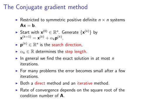
The Conjugate gradient method
I Restricted to symmetric positive definite n × n systemsAx = b.
I Start with x(0) ∈ Rn. Generate {x(k)} byx(k+1) = x(k) + αkp(k),
I p(k) ∈ Rn is the search direction,
I αk ∈ R determines the step length.
I In general we find the exact solution in at most niterations.
I For many problems the error becomes small after a fewiterations.
I Both a direct method and an iterative method.
I Rate of convergence depends on the square root of thecondition number of A.
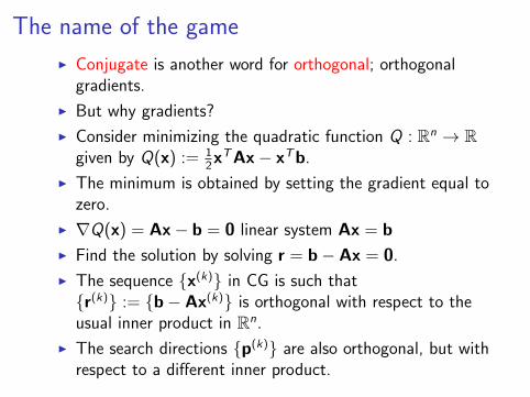
The name of the game
I Conjugate is another word for orthogonal; orthogonalgradients.
I But why gradients?
I Consider minimizing the quadratic function Q : Rn → Rgiven by Q(x) := 1
2xTAx− xTb.
I The minimum is obtained by setting the gradient equal tozero.
I ∇Q(x) = Ax− b = 0 linear system Ax = b
I Find the solution by solving r = b− Ax = 0.
I The sequence {x(k)} in CG is such that{r(k)} := {b− Ax(k)} is orthogonal with respect to theusual inner product in Rn.
I The search directions {p(k)} are also orthogonal, but withrespect to a different inner product.
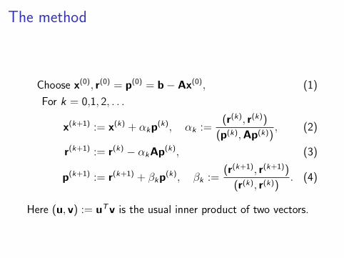
The method
Choose x(0), r(0) = p(0) = b− Ax(0), (1)
For k = 0,1, 2, . . .
x(k+1) := x(k) + αkp(k), αk :=
(r(k), r(k))
(p(k),Ap(k)), (2)
r(k+1) := r(k) − αkAp(k), (3)
p(k+1) := r(k+1) + βkp(k), βk :=
(r(k+1), r(k+1))
(r(k), r(k)). (4)
Here (u, v) := uTv is the usual inner product of two vectors.
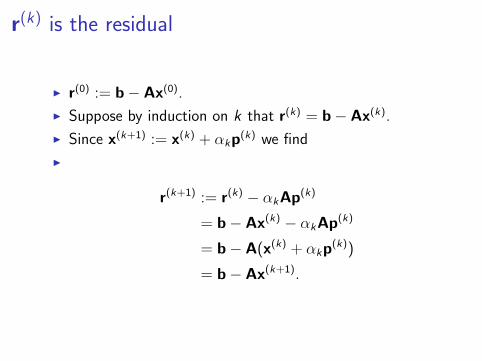
r(k) is the residual
I r(0) := b− Ax(0).
I Suppose by induction on k that r(k) = b− Ax(k).
I Since x(k+1) := x(k) + αkp(k) we find
I
r(k+1) := r(k) − αkAp(k)
= b− Ax(k) − αkAp(k)
= b− A(x(k) + αkp(k))
= b− Ax(k+1).
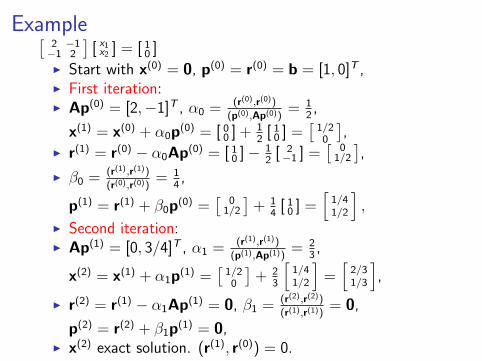
Example[2 −1−1 2
][ x1x2 ] = [ 10 ]
I Start with x(0) = 0, p(0) = r(0) = b = [1, 0]T ,I First iteration:I Ap(0) = [2,−1]T , α0 = (r(0),r(0))
(p(0),Ap(0))= 1
2,
x(1) = x(0) + α0p(0) = [ 00 ] + 12
[ 10 ] =[1/20
],
I r(1) = r(0) − α0Ap(0) = [ 10 ]− 12
[ 2−1 ] =
[0
1/2
],
I β0 = (r(1),r(1))(r(0),r(0))
= 14,
p(1) = r(1) + β0p(0) =[
01/2
]+ 1
4[ 10 ] =
[1/41/2
],
I Second iteration:I Ap(1) = [0, 3/4]T , α1 = (r(1),r(1))
(p(1),Ap(1))= 2
3,
x(2) = x(1) + α1p(1) =[1/20
]+ 2
3
[1/41/2
]=[2/31/3
],
I r(2) = r(1) − α1Ap(1) = 0, β1 = (r(2),r(2))
(r(1),r(1))= 0,
p(2) = r(2) + β1p(1) = 0,I x(2) exact solution. (r(1), r(0)) = 0.
Exact method and iterative method
I Orthogonality of the residuals implies that x(m) is equal tothe solution x of Ax = b for some m ≤ n.
I For if x(k) 6= x for all k = 0, 1, . . . , n − 1 then r(k) 6= 0 fork = 0, 1, . . . , n − 1 is an orthogonal basis for Rn. Butthen r(n) ∈ Rn is orthogonal to all vectors in Rn sor(n) = 0 and hence x(n) = x.
I So the conjugate gradient method finds the exact solutionin at most n iterations.
I The convergence analysis shows that x− x(k) typicallybecomes small quite rapidly and we can stop the iterationwith k much smaller that n.
I It is this rapid convergence which makes the methodinteresting and in practice an iterative method.
Conjugate Gradient Algorithm
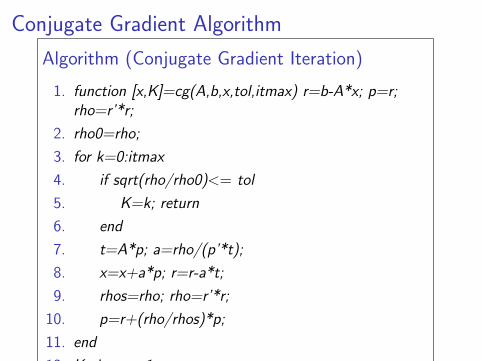
Algorithm (Conjugate Gradient Iteration)
1. function [x,K]=cg(A,b,x,tol,itmax) r=b-A*x; p=r;rho=r’*r;
2. rho0=rho;
3. for k=0:itmax
4. if sqrt(rho/rho0)<= tol
5. K=k; return
6. end
7. t=A*p; a=rho/(p’*t);
8. x=x+a*p; r=r-a*t;
9. rhos=rho; rho=r’*r;
10. p=r+(rho/rhos)*p;
11. end
12. K=itmax+1;
Complexity
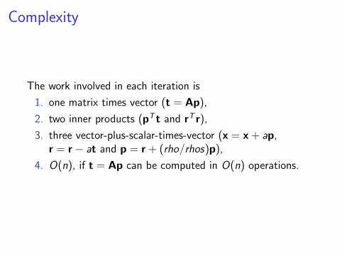
The work involved in each iteration is
1. one matrix times vector (t = Ap),
2. two inner products (pT t and rT r),
3. three vector-plus-scalar-times-vector (x = x + ap,r = r − at and p = r + (rho/rhos)p),
4. O(n), if t = Ap can be computed in O(n) operations.
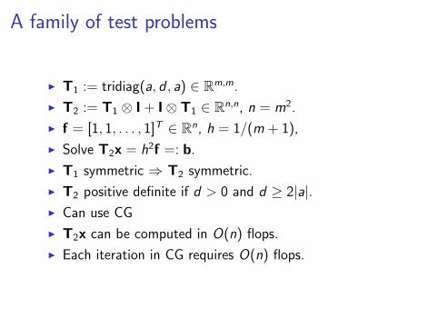
A family of test problems
I T1 := tridiag(a, d , a) ∈ Rm,m.
I T2 := T1 ⊗ I + I⊗ T1 ∈ Rn,n, n = m2.
I f = [1, 1, . . . , 1]T ∈ Rn, h = 1/(m + 1),
I Solve T2x = h2f =: b.
I T1 symmetric ⇒ T2 symmetric.
I T2 positive definite if d > 0 and d ≥ 2|a|.I Can use CG
I T2x can be computed in O(n) flops.
I Each iteration in CG requires O(n) flops.
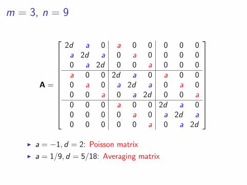
m = 3, n = 9
A =
2d a 0 a 0 0 0 0 0a 2d a 0 a 0 0 0 00 a 2d 0 0 a 0 0 0a 0 0 2d a 0 a 0 00 a 0 a 2d a 0 a 00 0 a 0 a 2d 0 0 a0 0 0 a 0 0 2d a 00 0 0 0 a 0 a 2d a0 0 0 0 0 a 0 a 2d
I a = −1, d = 2: Poisson matrix
I a = 1/9, d = 5/18: Averaging matrix
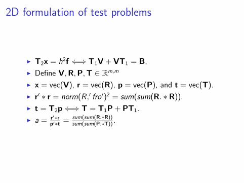
2D formulation of test problems
I T2x = h2f ⇐⇒ T1V + VT1 = B,
I Define V,R,P,T ∈ Rm,m
I x = vec(V), r = vec(R), p = vec(P), and t = vec(T).
I r′ ∗ r = norm(R ,′ fro ′)2 = sum(sum(R. ∗ R)).
I t = T2p⇐⇒ T = T1P + PT1.
I a = r′∗rp′∗t = sum(sum(R.∗R))
sum(sum(P.∗T)) .
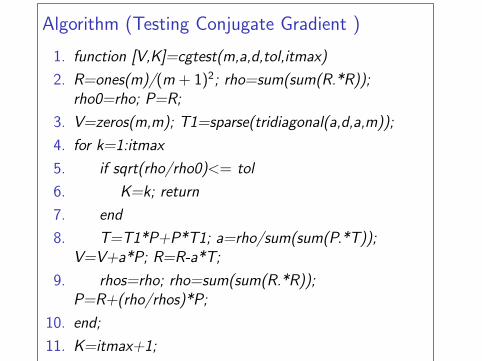
Algorithm (Testing Conjugate Gradient )
1. function [V,K]=cgtest(m,a,d,tol,itmax)
2. R=ones(m)/(m + 1)2; rho=sum(sum(R.*R));rho0=rho; P=R;
3. V=zeros(m,m); T1=sparse(tridiagonal(a,d,a,m));
4. for k=1:itmax
5. if sqrt(rho/rho0)<= tol
6. K=k; return
7. end
8. T=T1*P+P*T1; a=rho/sum(sum(P.*T));V=V+a*P; R=R-a*T;
9. rhos=rho; rho=sum(sum(R.*R));P=R+(rho/rhos)*P;
10. end;
11. K=itmax+1;
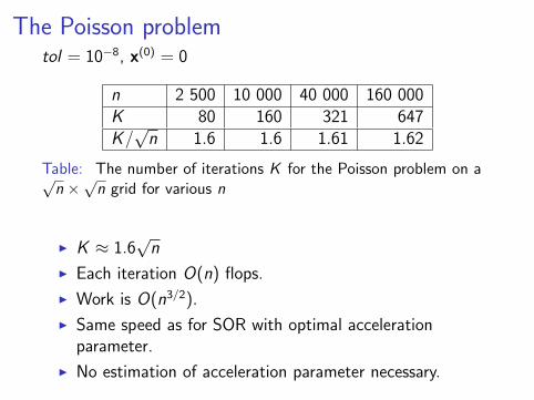
The Poisson problemtol = 10−8, x(0) = 0
n 2 500 10 000 40 000 160 000K 80 160 321 647K/√
n 1.6 1.6 1.61 1.62
Table: The number of iterations K for the Poisson problem on a√n ×√n grid for various n
I K ≈ 1.6√
n
I Each iteration O(n) flops.
I Work is O(n3/2).
I Same speed as for SOR with optimal accelerationparameter.
I No estimation of acceleration parameter necessary.
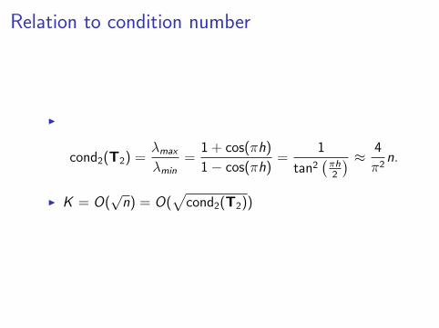
Relation to condition number
I
cond2(T2) =λmax
λmin=
1 + cos(πh)
1− cos(πh)=
1
tan2(πh2
) ≈ 4
π2n.
I K = O(√
n) = O(√
cond2(T2))
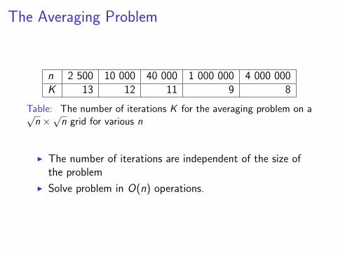
The Averaging Problem
n 2 500 10 000 40 000 1 000 000 4 000 000K 13 12 11 9 8
Table: The number of iterations K for the averaging problem on a√n ×√n grid for various n
I The number of iterations are independent of the size ofthe problem
I Solve problem in O(n) operations.
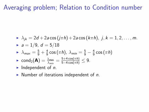
Averaging problem; Relation to Condition number
I λjk = 2d + 2a cos (jπh) + 2a cos (kπh), j , k = 1, 2, . . . ,m.
I a = 1/9, d = 5/18
I λmax = 59
+ 49
cos (πh), λmin = 59− 4
9cos (πh)
I cond2(A) = λmax
λmin= 5+4 cos(πh)
5−4 cos(πh) ≤ 9.
I Independent of n.
I Number of iterations independent of n.
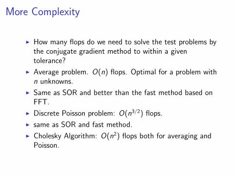
More Complexity
I How many flops do we need to solve the test problems bythe conjugate gradient method to within a giventolerance?
I Average problem. O(n) flops. Optimal for a problem withn unknowns.
I Same as SOR and better than the fast method based onFFT.
I Discrete Poisson problem: O(n3/2) flops.
I same as SOR and fast method.
I Cholesky Algorithm: O(n2) flops both for averaging andPoisson.
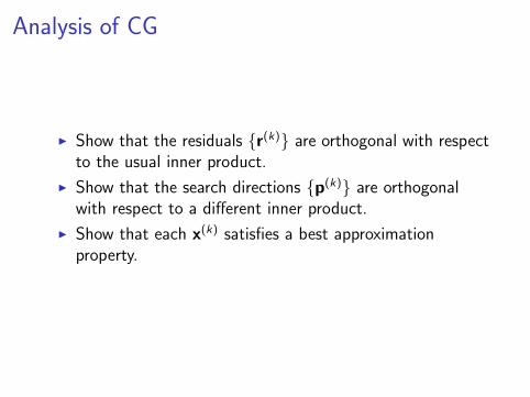
Analysis of CG
I Show that the residuals {r(k)} are orthogonal with respectto the usual inner product.
I Show that the search directions {p(k)} are orthogonalwith respect to a different inner product.
I Show that each x(k) satisfies a best approximationproperty.
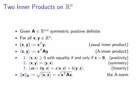
Two Inner Products on Rn
I Given A ∈ Rn,n symmetric positive definite.
I For all x, y ∈ Rn:
I (x, y) := xTy, (usual inner product)
I 〈x, y〉 := xTAy (A-inner product)
I 1. 〈x, x〉 ≥ 0 with equality if and only if x = 0. (positivity)2. 〈x, y〉 = 〈y, x〉 (symmetry)3. 〈ax+ by, z〉 = a〈x, z〉+ b〈y, z〉. (linearity)
I ‖x‖A :=√〈x, x〉 =
√xTAx. the A-norm
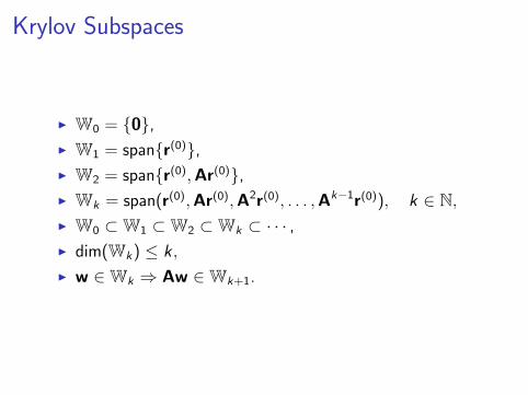
Krylov Subspaces
I W0 = {0},I W1 = span{r(0)},I W2 = span{r(0),Ar(0)},I Wk = span(r(0),Ar(0),A2r(0), . . . ,Ak−1r(0)), k ∈ N,I W0 ⊂W1 ⊂W2 ⊂Wk ⊂ · · · ,I dim(Wk) ≤ k ,
I w ∈Wk ⇒ Aw ∈Wk+1.
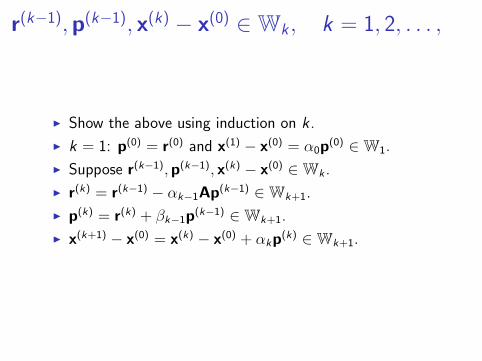
r(k−1),p(k−1), x(k) − x(0) ∈Wk , k = 1, 2, . . . ,
I Show the above using induction on k .
I k = 1: p(0) = r(0) and x(1) − x(0) = α0p(0) ∈W1.
I Suppose r(k−1),p(k−1), x(k) − x(0) ∈Wk .
I r(k) = r(k−1) − αk−1Ap(k−1) ∈Wk+1.
I p(k) = r(k) + βk−1p(k−1) ∈Wk+1.
I x(k+1) − x(0) = x(k) − x(0) + αkp(k) ∈Wk+1.
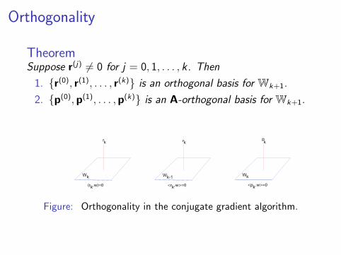
Orthogonality
TheoremSuppose r(j) 6= 0 for j = 0, 1, . . . , k. Then
1. {r(0), r(1), . . . , r(k)} is an orthogonal basis for Wk+1.
2. {p(0),p(1), . . . ,p(k)} is an A-orthogonal basis for Wk+1.
rk
Wk
(r , w)=0k
k
Wk-1
<r , w>=0k
r k
Wk
<p , w>=0
p
k
Figure: Orthogonality in the conjugate gradient algorithm.
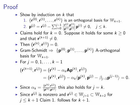
ProofI Show by induction on k that
1. {r(0), r(1), . . . , r(k)} is an orthogonal basis for Wk+1.
2. p(j) = r(j) −∑j−1
i=0〈r(j),p(i)〉〈p(i),p(i)〉p
(i) 6= 0, j ≤ k.
I Claims hold for k = 0. Suppose it holds for some k ≥ 0and that r(k+1) 6= 0.
I Then (r(k), r(i)) = 0.I Gram-Schmidt ⇒ {p(0),p(1), . . . ,p(k)} A-orthogonal
basis for Wk+1.I For j = 0, 1, . . . , k − 1
(r(k+1), r(j)) = (r(k) − αkAp(k), r(j))
= (r(k), r(j))− αk〈p(k),p(j) − βj−1p(j−1)〉 = 0.
I Since αk = (r(k),r(j))
〈p(k),p(j)〉 this also holds for j = k .
I Since r(j) is nonzero and r(j) ∈Wj+1 ⊂Wk+2 forj ≤ k + 1 Claim 1. follows for k + 1.
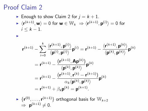
Proof Claim 2I Enough to show Claim 2 for j = k + 1.
I 〈r(k+1),w〉 = 0 for w ∈Wk ⇒ 〈r(k+1),p(i)〉 = 0 fori ≤ k − 1.
I
r(k+1) −k∑
i=0
〈r(k+1),p(i)〉〈p(i),p(i)〉
p(i) = r(k+1) − 〈r(k+1),p(k)〉〈p(k),p(k)〉
p(k)
= r(k+1) − (r(k+1),Ap(k))
〈p(k),p(k)〉p(k)
= r(k+1) − (r(k+1), r(k) − r(k+1))
αk〈p(k),p(k)〉p(k)
= r(k+1) + βkp(k) = p(k+1).
I {r(0), . . . , r(k+1)} orthogonal basis for Wk+2
⇒ p(k+1) 6= 0.
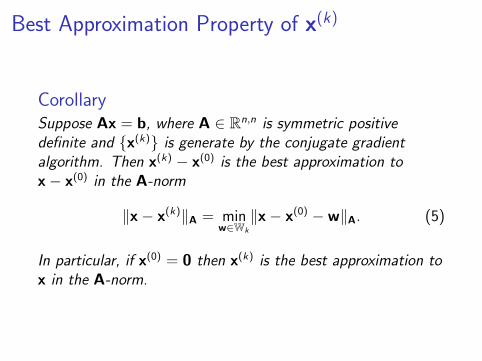
Best Approximation Property of x(k)
CorollarySuppose Ax = b, where A ∈ Rn,n is symmetric positivedefinite and {x(k)} is generate by the conjugate gradientalgorithm. Then x(k) − x(0) is the best approximation tox− x(0) in the A-norm
‖x− x(k)‖A = minw∈Wk
‖x− x(0) −w‖A. (5)
In particular, if x(0) = 0 then x(k) is the best approximation tox in the A-norm.
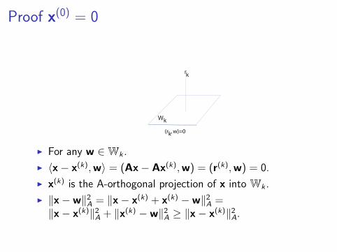
Proof x(0) = 0
rk
Wk
(r , w)=0k
I For any w ∈Wk .
I 〈x− x(k),w〉 = (Ax− Ax(k),w) = (r(k),w) = 0.
I x(k) is the A-orthogonal projection of x into Wk .
I ‖x−w‖2A = ‖x− x(k) + x(k) −w‖2A =‖x− x(k)‖2A + ‖x(k) −w‖2A ≥ ‖x− x(k)‖2A.
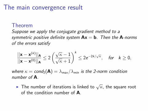
The main convergence result
TheoremSuppose we apply the conjugate gradient method to asymmetric positive definite system Ax = b. Then the A-normsof the errors satisfy
||x− x(k)||A||x− x(0)||A
≤ 2
(√κ− 1√κ + 1
)k
≤ 2e−2k/√κ, for k ≥ 0,
where κ = cond2(A) = λmax/λmin is the 2-norm conditionnumber of A.
I The number of iterations is linked to√κ, the square root
of the condition number of A.