The Project for Improvement of Road Technology in Disaster ...open_jicareport.jica.go.jp/pdf/12237533.pdf · 6.7.5 Peg for deformation survey ... as a sample case for practical calculation;

Republic of the Union of Myanmar Ministry of Construction, PW

The Project for Improvement of Road Technology

in Disaster Affected Area in Myanmar

Text Books for Practical Training about Checking Methods for Stability & Settlement

of High Embankment on Soft Ground

February 2015

Japan International Cooperation Agency （JICA）

Pegasus Engineering Corporation Oriental Consultants Global Co., Ltd.

EI

JR

15-151

Republic of the Union of Myanmar Public Works, Ministry of Construction

Textbook

For Practical Training

about Checking Methods

For Stability & Settlement

of High Embankment

on Soft Ground

February 2015 (R1)

PW, MOC, JICA

The Project for Implement of Road Technology

in Disaster Affected Area in Myanmar

Table of Contents 1. Preface ............................................................................................................... 1

2. Flow of Solution ................................................................................................. 2

3. Data collection for Basic Design......................................................................... 3 3.1 Necessary data for the stability analysis ................................................................ 3 3.2 Preparation of Data for “Consolidation Settlement” analysis ................................. 3

4. Stability Analysis ............................................................................................... 4 4.1 Precondition ........................................................................................................... 4 4.2 Assumption of ground earth stratum ...................................................................... 5 4.3 Assuming of shape of embankment ...................................................................... 12 4.4 Practice for the calculation ................................................................................... 14 4.5 Excel soft analysis methods .................................................................................. 15 4.6 EXCEL Methods (A) by Free application .............................................................. 18 4.7 EXCEL methods (B) by Free application .............................................................. 20 4.8 EXCEL methods (C) ............................................................................................. 21 4.9 GeoStudio Slope/W ............................................................................................... 22

4.9.1 Analysis for embankment with berms by Geo Studio .......................................23 4.10 Analysis for Multi-layer ground .......................................................................... 23 4.11 Summary ............................................................................................................ 23

5. Settlement Analysis ......................................................................................... 24 5.1 Preparation of Curves for Analysis ....................................................................... 25 5.2 Collection of data for “consolidation settlement calculation” ................................ 26

5.2.1 Consolidation Test ..............................................................................................26 5.2.2 Consolidation Characteristics Graphs to be prepared by Soil Laboratory Test27

5.3 Loading condition and geological stratum condition ............................................. 31 5.4 Settlement analysis .............................................................................................. 32

5.4.1 Calculation of effective stress on the settlement targeted strata .....................33 5.4.2 Calculation of consolidation settlement .............................................................34 5.4.3 Calculation of settlement time ...........................................................................38 5.4.4 Settlement Curve Modification based on Filling Rate ......................................41 5.4.5 Case study by Kywe Chan Ye Kyaw Bridge Project ..........................................42

6. Behavior Observation during Construction ..................................................... 43 6.1 Outline of the targeted Construction .................................................................... 44 6.2 Outline of Observation methods ........................................................................... 47 6.3 Measurement method of observation and necessary instruments ........................ 48 6.4 Procurement of Equipment ................................................................................... 50 6.5 Arrangement plan of observation Instrument ...................................................... 51 6.7 Setting of instrument ........................................................................................... 52

6.7.1 Settlement Plate: ................................................................................................52 6.7.2 Pour water pressure measurement device ........................................................52 6.7.3 Inclinometer guide pipe ......................................................................................53 6.7.4 Water level measurement well ...........................................................................53 6.7.5 Peg for deformation survey ................................................................................54

6.8 Observation, measurement and record ................................................................. 55 6.9 Observation results Reporting .............................................................................. 55 6.10 Example of the data processing of Measurement results .................................... 56 6.10.1. 3-D measurement ........................................................................................... 56 6.10.2 Settlement Plate .............................................................................................. 57 6.10.3 Inclinometer .................................................................................................... 58

6.10.4 Pore pressure meter .........................................................................................59 6.10.5 Underground Water level .................................................................................60

6.11 Analysis of obtained data & usage ...................................................................... 61

7. Study about Countermeasure .......................................................................... 63 7.1 Countermeasure study at each stage .................................................................... 63

7.2 Necessary countermeasure study for Stability during construction ....................63 7.3 Necessary countermeasure for settlement work ................................................... 64 7.4 List of Countermeasures to be taken in general ................................................... 64

7.4.1 Preloading method:(Surcharge method, Extra banking method) .....................66 7.4.2 Vertical drainage construction method (Sand Pile) ...........................................67

7.5 Feedback to construction works ............................................................................ 68 Annex ......................................................................................................................... 71

Annex 1 Brief explanation about using of Geostudio Annex 2 Inquiry about further information of GeoStudio Annex 3 Formula used in Excel sheet Annex 4: Excel method modified “C” to maximum 5 layers. Annex 5: Organized way of consolidation test results Annex 6: Consolidation Curve and yield point on an e-log P curve Annex 7: Plotting of log mv- log p curve Annex 8: Sample of obtaining e-log p curve by MS Excel Annex 9: Sample of obtaining Cv and Cv – P curve by MS Excel Annex 10: JIS Data Format Sheets Annex 11. Schedule of Approach embankment with Observation Plan Annex 12. Sample of Table contents for Observation analysis result report Annex13 (sample) Specification of Embankment at Approach Road to Bridges Annex 14: Answer of Drills

pg. 1

1. Preface

On construction of a high embankment on a soft ground, it is important to proceed with cautious manner. Especially in Ayeyarwady delta area, various kinds of issues is anticipated such as, slope instability during construction, consolidation settlement during and after construction.

Approach sections to bridge abutments in Ayeyarwady delta area have following issues to be solved: Big bump at the connection with abutment

Settlement of embankment

Sliding failures of the slope of embankment

Collapse of slope due to the erosion by the rain or water

These failures come mainly from following reasons: Inappropriate design

No countermeasures for soft soil treatment

Usage of poor materials for filling

Poor compaction methods

No countermeasures for slope protection

“Soft Ground Treatment Manual” is prepared, based on Japanese Soft Ground Treatment Manual, under Technical Cooperation Project for Implement of Road Technology in Disaster Affected Area in Myanmar. It contains almost of subject about soft ground treatment, such as definition, investing, analysis, design, countermeasures, treatment, work control and maintenance. It is comprehensive and rather theoretical.

While, this Practical Training Manual is prepared focusing the solution of such settlement with the stability analysis of high embankment as a supplementary one for the “Soft Soil Ground Treatment Manual”. This Manual is the summary of the Text Book used in the workshops, which were executed more than 15 times during the period of 2014 at Soil Research laboratory, Yangon.

This manual includes drills in some page to confirm the knowledge or understanding degree of the readers. Please try from time to time.

pg. 2

2. Flow of Solution

In order to solve the accident due to lack of stability and settlement, following procedures are required:

Fig 1 Flow chart of analysis

This manual describes a preliminary study method about the high embankment road on the soft ground as a sample case for practical calculation; high embankment approach road to Kywe Chan Ye Kyaw Bridge is used. Theoretical details are shown in Soft Ground Treatment Manual.

1. Collection of data

2. Assumption of ground earth stratum

3. Assuming of shape of embankment

4. Stability Calculation

5. Stability Factor > 1.25

6. Study about Countermeasure

7. Settlement Calculation

yes

no

8. Study about Settlement Countermeasure

9. Starting of construction

10. Behavior Observation

12. Continue the work and Completion

11. within Allowable limit

yes

no no

Design

Stability Analysis

Settlement Analysis

Observation during Construction

Drill 1: Connect by line, which has direct relations. (Max. line number is 6) * Internal friction angle

Ground settlement * * Inclinometer * Consolidation test

Slope stability * * Settlement Board * Pore pressure gauge

5. Stability Factor

11. within Allowable limit

yes

pg. 3

3. Data collection for Basic Design

3.1 Necessary data for the stability analysis

In order to carry out analysis work, it is necessary to execute soil investigation, which include laboratory test. Table 1 shows necessary data for the stability analysis:

Table 1 Necessary data for the stability calculation Data to be checked Remarks

Plan & Profile of embankment

Longitudinal slope Surrounding area conditions

Prepared date is important

Typical Cross section of Embankment

Top level height Bottom level height Slope inclination Berm width

Absolute height from B.M.

Bridge abutment cross section

Top level height Bottom level height

Boring log Each layer thickness for calculation

3.2 Preparation of Data for “Consolidation Settlement” analysis

The essential items for consolidation settlement are followings: 1. T Height (Thickness) of Soft stratum 2. ei Initial void ratio, 4. Pi Initial load pressures, 3. ef Void ratio after embankment load 5. Pf Load pressure after

embankment 8. Cc Compression coefficient 6. ∆P Increased load 9. mv Volume compression coefficient 7. Pc Pressure at yield point 10. Cv Consolidation coefficient

Right diagram shows process for soil investigation consolidation calculation. Soil Laboratory test report includes physical, mechanical and consolidation characteristics of each soil layers. Standard test record form for “ Consolidation test by step loading JIS（A1217）” is shown at Annex 1.

Fig 2 Process of Soil Investigation

Standard format for test results

Boring Survey

Laboratory Test

Shearing test

Preparation of Curves (Details in figure on next page)

N-Value

Sampling ( ) Visual checking

Soil property

Consolidation test

e-log p curve

log mw-log p curve

d-√𝑡 curve

Transportation to Lab

Consolidation-Time curve

Reporting of Laboratory Testing Results

pg. 4

4. Stability Analysis

4.1 Precondition

On the calculation of stability, we should consider following two facts: 1) The past research has considerably elucidated ground processes from

deformation to failure and the process of long-term settlement, however prediction of the behavior of the entire ground is not yet established as a practical method. It is necessary to be aware of the limitations, advantages, and disadvantages of the analysis theory.

2) Investigation and judgments are done based on the understanding that the values resulting from design or study contain some uncertainties.

3) It is necessary to recognize the possible errors of soil exploration data. Because, the soil samples are disturbed on taking and on transporting. And soil testing will be carried out under restricted conditions. Accurate information of the ground is difficult to know.

In this manual, followings are not included: Excluded item Remarks

1 Long slope corruption Analysis for cliff or steep slope 2 Mud ground Qc (Cone Index) < 200kN/m2 3 River & Seashore dike Note Pore pressure is required for land sliding analysis.

However, in case of embankment on soft ground, pore pressure is ignored.

――――――――――――――――――

Drill 2: Connect by line, which has direct relations. (Max. line number is 7) * Visual inspection

Original Ground strength * * CBR New Embankment strength * * N-value

Pavement strength * * Cone Penetration value * K-value

pg. 5

4.2 Assumption of ground earth stratum

Stratum of target earth ground shall be divided into a few layers from boring data.

As shown in bellow figure, shear stress is apt to concentrate to the slope toe. And usually, the bottom line of sliding circle will not pass the deep place.

Therefore, necessary soil stratum for analysis is for shallow places, not necessary up to deep layers.

Figure 5 (on p.6) shows an example of boring stratum of Kywe Chan Ye Kyaw Bridge. Table 2 (p.7&8) shows an example of their laboratory data. However, the data is not described by SI unit (International standard unit). All data shall be converted to SI unit on analyzing by popular soft wear.

From two kinds of data (boring stratum and laboratory data), each strata shall be classified to typical a few layers, and decide the typical characteristic data.

Table 3 (p.9&10) shows the converted results to SI unit.

Figure 6 (p.11) shows an example of dividing results of each stratum with typical each characteristic data. The finally decided typical cross section of soil stratum is shown in the Fig 4 as an example based on the comparison of two boring data, which are located in 50 meters distances as shown in Fig 7 (p.12). Soil layers are seemed to be almost horizontal.

On dividing the stratum, it is recommended to list up all kinds of available soil characteristic data in parallel (as shown in Fig 4) in order to know the property of stratum comprehensively. ----------------------------------------------------------- Note: In case of Kywe Chan Ye Kyaw bridge approach road, the top 1.5m layer of the boring data is the newly embanked road after Nargis. This road is banked in a rainy season without compaction. As the density of the road is very poor, PW has decided to replace the top soil to ensure the stability.

3.0m

2m~3.5m

Poor & Replace

γ w γd C Φ17,13,24,05

17,11,10,10

19,14,26,22

18,14,04,32

Fig 4. Decided typical cross section of soil stratum

as shown in the right side of Fig 6

Fig 3

pg. 6

Fig 5 Original Boring data (Kywe Chan Ye Kyaw Bridge 2014) , B1 location is 10m from abutment, and B2 is 60m.

pg. 7

Table 2-1 Original data of Laboratory Test Results – Kywe Chan Ye Kyaw Bridge A1 side approach section Boring No1

SAMPLE

depth Moisture Density USC Test

data SPT cohesive internal

SHELBY SPLIT Soil Classification contents wet dry strength strain strength friction No. No. (m) % Ibs/cu.ft Ibs/cu.ft Ibs/sq.ft % Blows/ft Ibs/sq.ft deg-min

1 0-0.65 . Light Greyish Brown Clayey SILT trace Sand 36.3 107.9 79.2 Not

amenable for U.C.S Test 4 275 4.45

UD(1) 1.5-1.95 Light Brownish Grey Clayey SILT trace Sand 35.5 108.4 80 1520 20 UD 500 5.00

1 3-3.65 Light Brownish Grey Clayey SILT trace Sand 34.4 116.8 86.9 2200 11.3 11

UD(2) 4.5-4.95 Grey Clayey SILT some fine Sand 45.4 105.1 72.3 380 20 UD 200 10.15

2 6.1-6.70 Grey Silty & Clayey fine SAND 29.5 114 88 950 17.5 7 550 21.30

2 7.62-8.05 Grey SAND some Silt 20.2 114.3 95.1 Not amenable for U.C.S Test 12

3 9.15-9.6 Grey SAND some Silt trace Clay 18.1 116.4 98.6 Not

amenable for U.C.S Test 20 80 32.00

4 12.2-12.65 Grey SAND some Silt trace Clav 10.5 126.3 114.3 Not

amenable for U.C.S Test 55

5 15.24-15.69 Grey SAND some Silt 15.6 120.7 104.4 Not amenable for U.C.S Test 26 30 34.45

6 18.29-18.74 Dark Grey SAND some Silt 19.1 114.3 96 Not amenable for U.C.S Test 32

pg. 8

Table 2-2 Original data of Laboratory Test Results – Kywe Chan Ye Kyaw Bridge A1 side approach section Boring No2

SAMPLE


data cohesive internal SHELBY SPLIT Soil Classification contents wet dry strength strain SPT strength friction

No. No. (m) % Ibs/cu.ft Ibs/cu.ft Ibs/sq.ft % Blows/ft Ibs/sq.ft deg-min

1 0-0.65 . Light Greyish Brown Clayey SILT trace Sand 11.8 120.4 107.7 Not

amenable for U.C.S

Test 6 520 5.15

UD(1) 1.5-1.95 Greyish Brown Clayey SILT trace Sand 35.4 109.1 80.6 1550 20 UD 225 10.30

1 3-3.65 Light Brownish Grey Clayey SILT trace Sand 33.6 115.7 86.6 1690 15 8

UD(2) 4.5-4.95 Grey Clayey SILT some fine Sand 42.6 16.2 74.5 420 20 UD 450 14.00

2 6.1-6.70 Grey Clayey SILT some fine Sand 27.4 118.5 93 1700 15 6

2 7.6-8.1 Grey SAND & Clayey Sand 23.9 112.9 91.1 Not

amenable for U.C.S

Test 11 650 22.00

3 9.15-9.6 Grey SAND & Clayey Sand 23.6 113.7 92 Not

amenable for U.C.S

Test 18

4 10.67-11.12 Grey SAND some Silt 15.6 121.1 104.8 Not amenable

for U.C.S Test 41 35 35.15

5 12.2-12.65 Grey SAND some Silt 14.8 120.9 105.3 Not amenable

for U.C.S Test 50

6 15.24-15.69 Grey SAND some Silt trace Clay 19.7 113.8 95.1 Not

amenable for U.C.S

Test 31 90 31.00

7 18.29-18.74 Grey SAND some Silt 18.8 115.2 97 Not amenable

for U.C.S Test 31

pg. 9

Table 3-1 Converted data of Laboratory Test Results – Kywe Chan Ye Kyaw Bridge A1 side approach section Boring No1

SAMPLE


data SPT cohesive internal SHELBY SPLIT Soil Classification contents wet dry strength strain strength friction

No. No. (m) % kN/m3 kN/m3 kN/m2 % Blows/ft kN/m2 deg

1 0-0.65 . Light Greyish Brown Clayey SILT trace Sand 36 17 12 Not

amenable for U.C.S

Test 4 13 5

UD(1) 1.5-1.95 Light Brownish Grey Clayey SILT trace Sand 36 17 13 73 20 UD 24 5

1 3-3.65 Light Brownish Grey Clayey SILT trace Sand 34 18 14 105 11.3 11

UD(2) 4.5-4.95 Grey Clayey SILT some fine Sand 45 17 11 18 20 UD 10 10

2 6.1-6.70 Grey Silty & Clayey fine SAND 30 18 14 46 17.5 7 26 22

2 7.62-8.05 Grey SAND some Silt 20 18 15 Not amenable

for U.C.S Test 12

3 9.15-9.6 Grey SAND some Silt trace Clay 18 18 16 Not

amenable for U.C.S

Test 20 4 32

4 12.2-12.65 Grey SAND some Silt trace Clav 11 20 18 Not

amenable for U.C.S

Test 55


for U.C.S Test 26 1 35

6 18.29-18.74 Dark Grey SAND some Silt 19 18 15 Not

amenable for U.C.S

Test 32

pg. 10

Table 3-2 Converted data of Laboratory Test Results – Kywe Chan Ye Kyaw Bridge A1 side approach section Boring No2

SAMPLE


data cohesive internal SHELBY SPLIT Soil Classification contents wet dry strength strain SPT strength friction

No. No. (m) % kN/m3 kN/m3 kN/m2 % Blows/ft kN/m2 deg

1 0-0.65 . Light Greyish Brown Clayey SILT trace Sand 12 19 17 Not

amenable for U.C.S

Test 6 25 5

UD(1) 1.5-1.95 Greyish Brown Clayey SILT trace Sand 35 17 13 74 20 UD 11 11

1 3-3.65 Light Brownish Grey Clayey SILT trace Sand 34 18 14 81 15 8

UD(2) 4.5-4.95 Grey Clayey SILT some fine Sand 43 17 12 20 20 UD 22 14

2 6.1-6.70 Grey Clayey SILT some fine Sand 27 19 15 81 15 6

2 7.6-8.1 Grey SAND & Clayey Sand 24 18 14 Not

amenable for U.C.S

Test 11 31 22

3 9.15-9.6 Grey SAND & Clayey Sand 24 18 15 Not

amenable for U.C.S

Test 18


for U.C.S Test 41 2 35


for U.C.S Test 50

6 15.24-15.69 Grey SAND some Silt trace Clay 20 18 15 Not

amenable for U.C.S

Test 31 4 31


for U.C.S Test 31

pg. 11

Fig 6 Classified results of each stratum with each characteristic data (Kywe Chan Ye Kyaw Bridge 2014).

GL: 100.2Ft=30.54m1st Layer 4.92Ft = 1.5 m

γw γd C Φ Uc

19, 16, 01, 35,

20, 18, --, --, --

18, 15, 04, 32,

18, 14, 26, 22, 45

18, 15, --, --, --

17, 11, 10, 10, 18

17, 13, 24, 05, 73

18 14 105

GL: 99.7Ft=30.39m1st Layer 4.92Ft = 1.5 m

γw γd C Φ Uc

17, 13, 24, 05, 74

18, 14, --, --, 81

18, 15, 04, 31,

19, 16, 02 35, --

19, 17, --, --, --

18, 14, --, --, --

19, 15, 22, 14, 81

18, 14, 31, 22, --

17, 12, 11 11, 20

Assumed Soil Stratum &

their property data for

calculation

- 1.5m

119, 155 222 14 81

- 4.5m

- 6.0m

- 7.0m

- 9.0m~

1.5m

3.0m

1.5m

1.0m

2m~3.5m

Poor & Replace

γw γd C Φ17,13,24,05

17,11,10,10

19,14,26,22

18,14,04,32

pg. 12

4.3 Assuming of shape of embankment

Cross section of embankment shall be assumed to check the stability of the embankment.

Bellow figures are example of plan1 and cross section of Kywe Chan Ye Kyaw bridge approach road.

Fig 7 Pan, Profile & Cross section of Kywe Chan Ye Kyaw Bridge

1 Shapes of Plan are different. Upper one by RRL. Lower one by TCP team.

River Side →

10.0 m50.0 m

128.84Ft=39.27m120.64Ft=36.77m

GL: 100.2Ft=30.54mΔH: 28.64 = 8.73m1st Layer 4.92Ft = 1.5 mBank H 33.56Ft= 10.23m

GL: 99.7Ft=30.39mΔH: 20.94 = 6.381st Layer 4.92Ft = 1.5 mBank H 25.86Ft= 7.88m

pg. 13

Fig 8 shows the assumed typical cross sections at Boring No.1 location for the stability calculation from above drawings as follows: ( ) shows points’ coordinates.

Fig 8 assumed typical cross sections for the stability calculation

1:1

1:1.5

1:2

H=3.5m

H=3.4m

H=3.4m

L=6.1m

L=5.3m L=5.0m L=6.7m

(0,0)

(0, 10.3)

(6.1, 0) (11.4, 0) (14.4, 0) (19.4, 0) (22.4, 0) (29.1, 0)

(22.4, 3.4) (19.4, 3.4)

(14.4, 6.8) (11.4, 6.8)

(6.1, 10.3)

Drill 10: Visual shear strength is presented by internal friction angle in case of Sand and by cohesion in case of Clay. This is correct or not correct ?

Drill 9: If there is adhesion, cohesion will be added to shear strength. This is correct or not correct ?

Drill 8: Real shear strength is produced by internal friction angle not only for Sand but

also for Clay. This is correct or not correct ?

Drill 4: Internal friction angle φ is minimum 45 degree.

This is correct or not correct ?

Drill 5: Shear strength will be produced by the friction strength of soil particles, and

shear strength is zero, if there is no overburden pressure.


Drill 6: Shear strength of Clay is produced by cohesion only.


Drill 7: Shear strength of Sand is produced by internal friction angle.


pg. 14

4.4 Practice for the calculation

There are many kinds of slope stability analysis Program2.

Almost of landslide disasters, such as Slope slide, Rock falling, Large-scale Land slide and Avalanche etc. are not circular slip. However, in case of analysis of Slope Slide, circular slip type is adopted from the past actual disaster analysis.

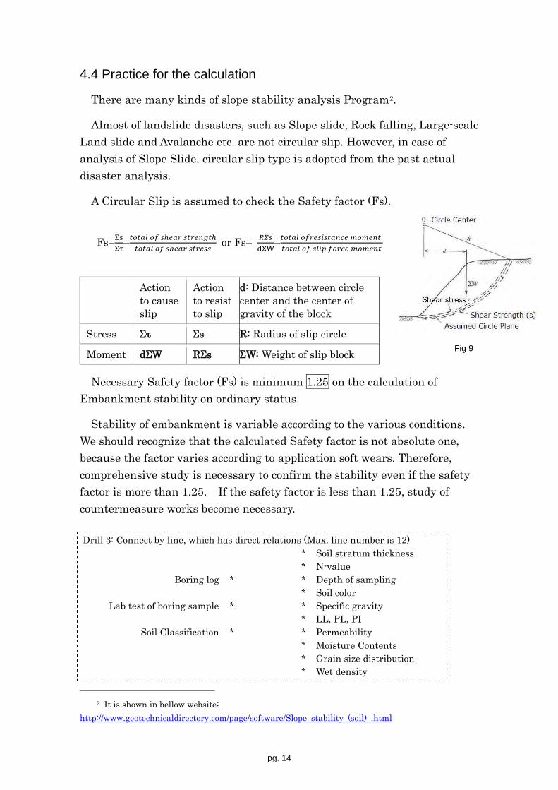
A Circular Slip is assumed to check the Safety factor (Fs).

Fs=ΣsΣτ

=𝑡𝑜𝑡𝑎𝑙 𝑜𝑓 𝑠ℎ𝑒𝑎𝑟 𝑠𝑡𝑟𝑒𝑛𝑔𝑡ℎ𝑡𝑜𝑡𝑎𝑙 𝑜𝑓 𝑠ℎ𝑒𝑎𝑟 𝑠𝑡𝑟𝑒𝑠𝑠

or Fs= 𝑅𝛴𝑠dΣW

=𝑡𝑜𝑡𝑎𝑙 𝑜𝑓𝑟𝑒𝑠𝑖𝑠𝑡𝑎𝑛𝑐𝑒 𝑚𝑜𝑚𝑒𝑛𝑡 𝑡𝑜𝑡𝑎𝑙 𝑜𝑓 𝑠𝑙𝑖𝑝 𝑓𝑜𝑟𝑐𝑒 𝑚𝑜𝑚𝑒𝑛𝑡

Action

to cause slip

Action to resist to slip

d: Distance between circle center and the center of gravity of the block

Stress Στ Σs R: Radius of slip circle

Moment dΣW RΣs ΣW: Weight of slip block

Necessary Safety factor (Fs) is minimum 1.25 on the calculation of Embankment stability on ordinary status.

Stability of embankment is variable according to the various conditions. We should recognize that the calculated Safety factor is not absolute one, because the factor varies according to application soft wears. Therefore, comprehensive study is necessary to confirm the stability even if the safety factor is more than 1.25. If the safety factor is less than 1.25, study of countermeasure works become necessary.

2 It is shown in bellow website:

http://www.geotechnicaldirectory.com/page/software/Slope_stability_(soil)_.html

Drill 3: Connect by line, which has direct relations (Max. line number is 12) * Soil stratum thickness * N-value

Boring log * * Depth of sampling * Soil color

Lab test of boring sample * * Specific gravity * LL, PL, PI

Soil Classification * * Permeability * Moisture Contents * Grain size distribution * Wet density

Fig 9

http://www.geotechnicaldirectory.com/page/software/Slope_stability_(soil)_.html

pg. 15

4.5 Excel soft analysis methods

It is necessary to repeat the calculation to get the circular with minimum Fs as shown in bellow procedures:

Calculation of Seek Fs will be done by the following process.

Ground Line Y=0

Top Line Y=h

slope gradient (1:m)

slope shouder (mh,h)

Center of Circle

Radius Ro

Left End Point (XL,YL)

Right End Point (XR, YR)

Slice width w= (XR-XL)/n

Slice Number (n)

Slice1 center line X1= XL+w/2Slice1 bottom Y1= - ((Ro^2-(X1-X0) 2̂)^0.5)+Y0

Slice N center line Xn= Xn-1+wSlice1 bottom Ydn= - ((Ro^2-(Xn-Xo)^2)^0.5)+Yo

Repeat N-1 times

Table of Slice (Xn, Ydn)

Top cross point (Ynu) of each slice center lineYun=0 or Yun=Xn/m or Yun=h

Height of each slice Hn=Yun-Ydn

Area of each slice An=Hn*w

Weight of each slice Wn=An*γUnit Weight (γ)

Angle for each Slice

cos αn, sinαn

Ln=w/cos αnLn=w/cos αnCohision C

Ln=w/cos αn

Ln*c

Wn*sin α, Wn*Cos α

Wn*Cos α* tan φinternal frictionn φ

Assume circular center & R

Seek Fs Change R

(First X: center of slope, Y: Top of slope)

Get R with minimum Fs

(First R: up to the original ground level)

Change circular center

Prepare table showing FS as shown in right Figure

Get center with minimum Fs

Fig 10

Fig 11

pg. 16

Here definition of each point is shown in bellow figure:

Bellow figures are examples to find out the location of circle center. But this is applicable to the limited conditions.

Bellow figure shows other method to find out slope circle in case of toe failure.

Right

Leftt

Cross

Circle

α

width

α

length

Toe Point

length

αα

Fig 12

Fig 13

Fig 14

pg. 17

Excel is convenient for these repeating calculation.

However, analysis becomes complicate, if slope shape has berms and if the ground is with multiple layers.

This manual shows following 6 methods Analysis

by Max. Layer

Berm Figure draw

Remarks

Method A EXCEL 1 Without Automatic For initial introduction Method B EXCEL 1 Without Automatic To know relation R & Fs Method C EXCEL 2 Without none To master analysis methods Method D GeoStudio 3 Without Automatic Method D’ GeoStudio 3 With Automatic Method E EXCEL 5 Without none For reference in Annex

The bellow table shows the calculation data to be used as a training about Kywe Chan Ye Kyaw bridge approach road. (See Fig 4 on page 11.)

Embankment height =10.3m Soil Property of embankment γ=17kN/m3, C=24kN/m2, φ =5 First ground layer Thickness=3.0m γ=17kN/m3, C=24kN/m2, φ =5 Second ground layer Thickness=1.5m γ=17kN/m3, C=10kN/m2, φ =10 Third ground layer Thickness=1.0m γ=19kN/m3, C=26kN/m2, φ =22 Fourth ground layer Thickness=2.5m γ=18kN/m3, C=04kN/m2, φ =32 First Radius =10.3m Distance between top and bottom

level First Center points (11.5, 10.3) X: middle of slope,

Y: height of embankment

Following condition are adopted on this trial calculation: 1) Material of embankment is same as original ground considering the

actual site conditions. 2) If the layer number is limited on using the application soft wears, soil

property data for the deeper layer is assumed to be same as those of upper layer.

pg. 18

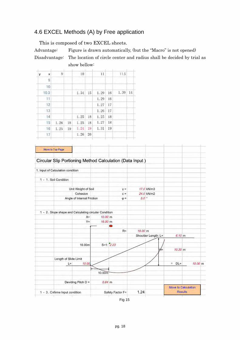
4.6 EXCEL Methods (A) by Free application

This is composed of two EXCEL sheets. Advantage: Figure is drawn automatically, (but the “Macro” is not opened) Disadvantage: The location of circle center and radius shall be decided by trial as

show bellow:

Fig 15

pg. 19

Calculation of Circular Slip by Portioning Method

§１. Design Condition

　１－１. Condition of Calculation

Unit Weight of Soil γ= 17.0 kN/m3Cohesion c= 24.0 kN/m2Angle of Internal Friction φ= 5.0 °

　１－２. Geometric Condition of Slip Circle

① Height of Slope H= 10.30 m DL= 10.000 m

② Centre Coordinate X= 20.00 Radius r= 19.00 mY= 26.00

③ Angle of Arch α= 105.1045 °

Back to Previous

§２ Calculation of Safety Factor

　２－１. Calculation of slip circle length

L= 2πr * α/360= 2*π*19.00 * 105.1045°/360= 34.88 m

　２－２. Calculation of Safety Factor

Fs= (cl+ΣWcosαtanφ) / ΣWsinα= (24.0*34.88+2745.517*tan(5.0))/867.292= 1.24

Fig 16

pg. 20

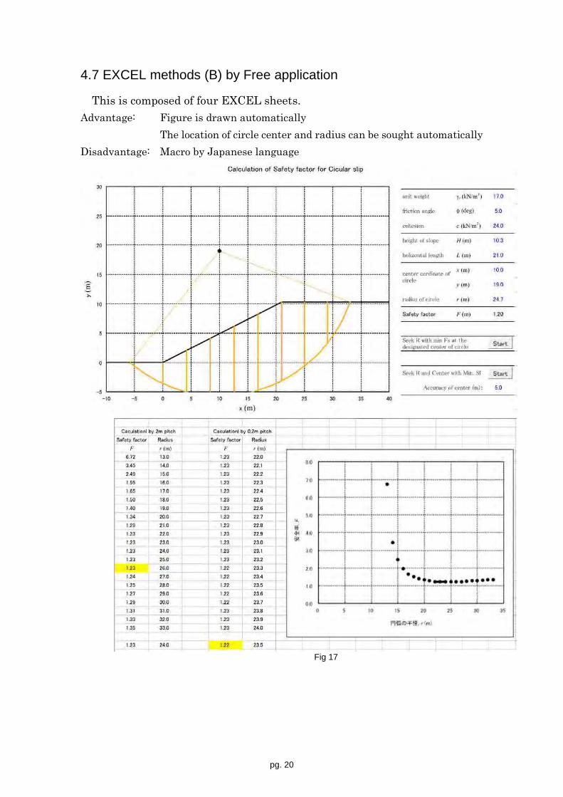
4.7 EXCEL methods (B) by Free application

This is composed of four EXCEL sheets. Advantage: Figure is drawn automatically

The location of circle center and radius can be sought automatically Disadvantage: Macro by Japanese language

Fig 17

pg. 21

4.8 EXCEL methods (C)

This is EXCEL analysis methods for embankment with 2 layers. Advantage: Changeable any cell Disadvantage: No automatic figure preparation system The location of circle center and radius shall be decided by trial

pg. 22

4.9 GeoStudio Slope/W

This is a standard application soft wear (Price is expensive as shown in bellow). However, “Student version” is available with free of charge.3

Bellow figure is a calculation results with following data: Unit Weight: Cohesion': Phi':

embankment 17 kN/m³ 24 kPa 5 ° layer2 17 kN/m³ 11 kPa 10 ° layer3 19 kN/m³ 26 kPa 22 °

In case of Kywe Chan Ye Kyaw Bridge approach embankment, embankment material is collected around the site. Therefore, the embankment materials and the 1st layer materials are assumed to be same. And the region of embankment and 1st layer was assumed to be same.

3 GeoStudio is useful, but expensive software, initial US$4450+ maintenance $ 900/year. However, “Student edition” is available with free of charge. “Student edition” has a limitation as show in right.

Number of multiple/staged analyses 2 Number of regions 10 Number of materials 3 Finite Element Integration 500 elements Analysis Methods Yes Ordinary Yes Bishop Simplified Yes Janbu Simplified Yes Morgenstern-Price Yes Spencer Yes

Convert

X 18.99 (6.1+23)-18.99=10.11

Y 25.88 25.88-10=15.88

Fig 18

pg. 23

4.9.1 Analysis for embankment with berms by Geo Studio

Below shows another analysis result for the same embankment with berms.

4.10 Analysis for Multi-layer ground

see Annex 4

4.11 Summary

Safety factors calculated from each methods will be summarized as follows:

Sf Circle center R(m) A) Excel methods A by Free application 1.24 10,16 19 B) Excel method B 1.20 10,19 25 C) Excel methods C 1.24 9,16 20 D) GeoStudio Slope/W without berms 1.27 10,16 20 D’) GeoStudio Slope/W with berms 1.30 10,16 20

It will be said that Sf is almost similar varying between 1.2 and 1.3. But, we could not say that the embankment is safety one from these stability values.

HOWEVER, the embankment material soil is mixed one with site soil and 30% of sand. It means that the safety factor could be increased due to the increasing of internal friction of embankment materials.

--------------------------------- Note: Fs between 4.9) without berm and 4.9.1) with berm are almost same. The value with berm is a little big.

Fig 19

pg. 24

5. Settlement Analysis

Settlement is unavoidable for the structure on soft ground.

Settlements are classified into 3 categories as follows: Kinds of settlement Brief Explanation

1 Immediate Settlement

Deformation will complete relatively & quickly after loading.

Resulting from shearing of a cohesive soil layer and resulting

from compression deformation of a loose sandy soil layer 2 Primary

consolidation settlement

This phenomenon will occur due to expulsion of pore water pressure, and directly affect to design and construction.

2 Secondary consolidation settlement

It is generally thought that “Secondary consolidation settlement” (creep) is due to changes in soil structure, although no reliable theory has been proposed as yet

This manual is prepared for the study about primary consolidation settlement.

It is expected following two facts on the analysis of consolidation settlement: 1) The past research has considerably elucidated ground processes from

deformation to failure and the process of long-term settlement, however prediction of the behavior of the entire ground is not yet established as a practical method. It is necessary to be aware of the limitations, advantages, and disadvantages of the analysis theory. Investigation and judgments are done based on the understanding that the values resulting from design or study contain some uncertainties.

2) It is necessary to recognize the possible errors of soil exploration data. Because, the soil samples are disturbed on taking and on transporting. And soil testing will be carried out under restricted conditions. Accurate information of the ground is difficult to know.4

4 Bellow table shows the difference of Cc and Pc point according to the analyzer. Comparison of each ones result (2014/11/24) Person 1 2 3 4 5 6 Cc 0.30 0.22 0.23 0.29 0.16 0,11 Yield pressure 1.65 120 190 89 45 165 Yield e 0.81 0.81 0.83 0.84 0.86 0.81

pg. 25

Drawings of longitudinal / cross-sectional and soil property data of embankment materials (such as unit weight) are necessary for the settlement analysis (refer section 3.3) as same as stability analysis.

After collecting all data, analysis will be conducted as shown in bellow Analysis Process Figure.

5.1 Preparation of Curves for Analysis

After calculation of settlement value and settlement time, if necessary, counter measure should be considered.

Compression curve methods

Collection of data Fill: Shape, Height Unit weight

Ground soil stratum Each layer: Thickness Unit weight

e-log p curve

d-√𝑡 curve (Tailor methods)

Consolidation-Time

Log mv-log p curve

Cc methods

mv methods

ei,ef

Cc, ei, Pf, Pi

Settlement value

Settlement time

mv, ∆p

Cv, Tu, U d-log t method

(Casagrande method)

Fitting method

T: Thickness of Soft stratum ei: initial void ratio, ef: void ratio after embankment Pi: initial load pressures, Pf: load pressure after embankment ∆P: increased load Pc: Pressure at yield point Cc: Compression coefficient mv: Volume compression coefficient Cv: Consolidation coefficient Tu: Time for Consolidation U: Consolidation rate (%)

Remarks:

LogCv-log P curve

This Analysis should be

done as laboratory work

T

Fig 20

pg. 26

5.2 Collection of data for “consolidation settlement calculation”

5.2.1 Consolidation Test

Consolidation test is a kind of model test carried out by creating a small specimen for clay taken from the field. The consolidation test container’s cross-sectional view is shown in bellow. Specimen height is only a few cm, which is very small comparing with actual soft ground stratum thickness.

Sequence of test procedures is as bellow:

As Testing Process

Sampling

Preparation of Specimen Diameter: 6cm

Height: 2cm

Put in Testing Equipment

Loading: P1=10kN/m2 Measurement of consolidation

value after each time of: t: 3, 6, 9, 12, 18, 30, 42(s)

1,1.5,2,3,5,7,10,15,20,30,40(min) 1,1.5,2,3,6,12,24 (hour)

Then changing load and repeat every time x2 load :

P1=20, 39, 78, - - - -up to 1255 kN/m2

Unloading Process

Calculation of Pore Ratio

measure Water Contents

measure Dry density ms of specimen

Fig 22 Sequence of Consolidation test by Stage Loading Process & Process of Data Acquisition

1. Draw d-t curve of P1=10kN/m2 2. Decision of e1 from final

consolidation value △d1 3. Decision of consolidation

coefficient Cv1 4. Calculation of volume

compression coefficient

measuring expanding value by reducing load up to

the first load of 10kkN/m2

Each loading Stage Whole loading Stage

Decision of Compression Index: Cc

Compression yield stress Pc*

Draw e-log p curve

Draw Log mv- log ṕ curve Log Cv-log P curve

D-√t curve

Mv, Cv,

*Pc (yield stress point) will be decided by the methods shown in ANNEX 2.

Fig 21

pg. 27

Notice

Load should be increased step by step by adding twice of the previous load. This is to plot the data at equal intervals on the axis of e-log p curves. Cycle for step loading is used 24 hours, so that load increase could be done at the same time each day. Though, Kyew Chan Ye Kyaw Approach Road Consolidation test had been applied following load steps as shown in upper line of bellow Table, it is recommended to add two more two loading steps in order to clearly identify the linear part of e-log p curve, which represent the steepest slope of the normal consolidation area.

Load to be applied (kN/m2) SRL methods 9.8 19.6 39.2 78.5 157 314 (None) (None)

Desirable 10 20 39 78 157 314 628 1255

5.2.2 Consolidation Characteristics Graphs to be prepared by Soil Laboratory Test

To read or obtain above data, following 3 curves for each stratum are necessary.

1. e-log p curve 2. log mv-log p curve 3. log Cv – log p curve

Fig-23 graphs are prepared by TCP Team from same report’s data. e-log P curve note: How to obtain this graph is shown in Annex 8

Kywe Chan Ye Kyaw Bridge Approach Road Soil investigation Report include e-log p curve only as a consolidation test data, which are shown in Fig-24;

Fig 23

pg. 28

e-log p curve for Boring No.1-2nd layer

log mv- log P relation

Note How to obtain this graph is shown in Annex 7

log Cv- log P curve

refer Appendix 9

logmv logP

logP

Log

Cv

Fig 24

Fig 25

Fig 26

pg. 29

To obtain each points of this Cv value in the graph, there are three methods:

From a following curve at left side seek values of right side connected by arrow. d-√t curve method,

1) d0 (mm):

Displacement corresponding to theoretical consolidation ratio 0%

d-log t curve method

2) d100 (mm):

Displacement corresponding to theoretical consolidation ratio 100%

d-log t curve fitting method 1) t90 (min)

Time corresponding to theoretical consolidation ratio 90% (in case of d-√t method)

2) t50 (min) Time corresponding to theoretical consolidation ratio 50% (in case of d-log t method)

(1) d-√t method: (Taylor’s method) 1) Make d-√t graph: dial gauge reading d(mm) at vertical axis, and elapsed

time t (min) on a horizontal axis with √t scale

2) As an initial correction point, which falls on t = 0 by extending the straight portions appearing in the initial portion of d-√t curve, and reading of this make it d0 (mm).

3) Draw a straight line having a lateral distance of 1.15 times the straight line through the initial correction point

4) Read a t90 (min) of the intersection with the d-√t curve and this straight line and make this point as a theoretical consolidation ratio 90%.

5) Calculate a d100 by following formula:d100 = 10/9 * (d90 -d0 )+ d0

(2) d-log t method (Casagrande’s method)

1) Make d-log t graph: dial gauge reading d(mm) at vertical axis, and elapsed time t (min) on a horizontal axis with log scale.

2) Draw two lines extending straight portion middle of d-log t and last part of

Fig 27

pg. 30

d-log t and make that intersection point as (d100, t100). 3) Select any point (t1, d1)

and (t2 =4*t1, d2) point on early portion of d-log t curve.

4) From above reading di, d2, obtain d0 by following relation: d1 - d0 =d2 - d1

5) Make it d50, half way between d0 and d100, Cc can be computed by following: Cc =0.197 x 1440 (H/2)2 / d50 (Unit: cm2/day)

(3) d-log t curve fitting method

1) Make d-log t graph: dial gauge reading d(mm) at vertical axis, and elapsed time t (min) on a horizontal axis with log scale.

2) Prepare a curve ruler drawn to log cycle of the same length as the one that drew a d-log t curve.

3) Overlay the curve ruler on the e-log t curve and move it parallel to up, down, left and right

4) Choose the one that matches the longest include the initial part of the d-log t curve.

5) Read d0 from theoretical consolidation degree 0 of the curve ruler. 6) Obtain t50 and t100 from the selected curve by above 4).

Sample of curve ruler

Length of 1 cycle

Fig 28

Fig 29

pg. 31

3.2 m

3.2 m

3.0 m

6.4 m6.0 m

4.8 m 4.5 m3.0 m3.0 m

CL

Cross Section of Embankment

21.7m

5.3 Loading condition and geological stratum condition

(1) Loading condition

Cross-section of the embankment and specific gravity of the fill material is required for obtain Loading condition; traffic load is also taken into account in some cases. As a sample, here shows Cross section of the Kywe Chan Ye Kyaw Bridge approach embankment:

H = 9.4 m (at the highest)

Horizontal length of Slope: Lh = 21.7m γ=1.7

(2) Geological stratum condition

Boring log of the Kywe Chan Ye Kyaw Bridge approach road is following:

From the soil layers data, it is assumed thickness of the clay layer and unit weight of soil to be the subject of settlement. Generally stratum of groundwater level above does not object consolidation settlement and specific gravity of the soil layer of below groundwater level is assumed minus the specific gravity of water.

Original Ground Level

h1=3m

h2=1.5m

h3=1.0m

Original Ground Level

N>10, Exclude from consolidation target l

Fig 30

Fig 31

pg. 32

5.4 Settlement analysis

Target soil for Subsidence of cohesive soil is about N value less than 10 and sand layer is not necessary to study for consolidation.

As a sample, here shows a highest point cross section of Kywe Chan Ye Kyaw Bridge Approach road.

Cross Section of Embankment

21.7m 6.1m

Embankment γ＝ 18 ｋN/m3H= 9.4 m

9.4 mStrata

3.0 m H= 3.0 γ＝ 71.5 γ′＝ 7

1.5 m 1.0 γ′＝ 81.0 m

9.4

3.01．Clayey Silt, trace Sand

1.52．Clayey Silt with fine Sand

CL

1.03．Clayey Silt with fine Sand

Primary Question

What is the definition of High embankment?

What will happen on High Embankment?

Why observation is necessary?

What will be measured by settlement plate?

What will be measured by Survey Peg?

What will be measured by Inclinometer?

What will be measured by Pore Pressure Gauge?

Why underground water level shall be measured?

Fig 32

pg. 33

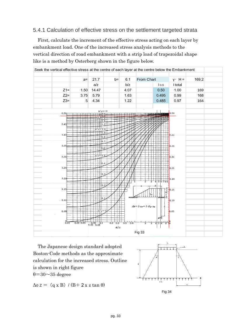
5.4.1 Calculation of effective stress on the settlement targeted strata

First, calculate the increment of the effective stress acting on each layer by embankment load. One of the increased stress analysis methods to the vertical direction of road embankment with a strip load of trapezoidal shape like is a method by Osterberg shown in the figure below.

The Japanese design standard adopted Boston-Code methods as the approximate calculation for the increased stress. Outline is shown in right figure θ＝30～35 degree

Δσｚ＝（q x B）/ (B＋２x z tan θ)

Seek the vertical effective stress at the centre of each layer at the centre below the Embankment

a= 21.7 b= 6.1 From Chart γ・H＝ 169.2a/z b/z I 0.5 I total

Z1= 1.50 14.47 4.07 0.50 1.00 169Z2= 3.75 5.79 1.63 0.495 0.99 168Z3= 5 4.34 1.22 0.485 0.97 164

Fig 33

Fig 34

pg. 34

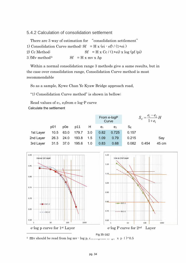
5.4.2 Calculation of consolidation settlement

There are 3 way of estimation for “consolidation settlement” 1) Consolidation Curve method: Sf = H x (ei - ef) / (1+ei ) 2) Cc Method: Sf = H x Cc / (1+ei) x log (pf /pi) 3 )Mv method5: Sf = H x mv x Δp

Within a normal consolidation range 3 methods give a same results, but in the case over consolidation range, Consolidation Curve method is most recommendable

So as a sample, Kywe Chan Ye Kyaw Bridge approach road,

“1) Consolidation Curve method” is shown in bellow;

Read values of e1, e2from e log-P curve Calculate the settlement

From e-logP Curve

p01 p0e p11 H e1 e2 SE

1st Layer 10.5 63.0 179.7 3.0 0.82 0.725 0.157 2nd Layer 26.3 24.0 193.8 1.5 1.09 0.79 0.215 Say 3rd Layer 31.5 37.0 195.6 1.0 0.83 0.68 0.082 0.454 45 cm

e-log p curve for 1st Layer e-log P curve for 2nd Layer

5 mv should be read from log mv - log p, correspond to (pi ｘｐｆ)^0.5

Fig 35-1&2

pg. 35

Note; Doted line in an e-log p curve indicates for Boring No.2

e-log p curve for 3rd Layer

As a comparison, “2) Cc Method” calculation result added on the right side of below table. For No1. Boring: (Same sample as the above e-log P method)

”3) mv method” calculation results are shown following table for a comparison,.

H (m) P1 P2 ΔP

(kN/m2) Geometric

Mean Mv(kN/m2) S(m)

1st Layer 3 11 183 172 44.9 2.20E-04 0.114 2nd Layer 1.5 26 198.8 172.8 71.9 1.10E-03 0.285 3rd Layer 1 32 204.6 172.6 80.9 6.00E-04 0.104

0.502

Geometric mean: (P1,P2) = (P1*P2)^(1/2)

Calculate the settlement

From e-logP Curvep01 p0e p11 H e1 e2 SE Cc S

1st Layer 10.5 63.0 179.7 3.0 0.82 0.725 0.157 0.209 0.1572nd Layer 26.3 24.0 193.8 1.5 1.09 0.79 0.215 Say 0.331 0.2153rd Layer 31.5 37.0 195.6 1.0 0.83 0.68 0.082 0.454 45 cm 0.207 0.082

(Say 45 cm) 45 cm

( )0

1001 p

pΔploge

hCS oc

++

=

Fig 35-3

pg. 36

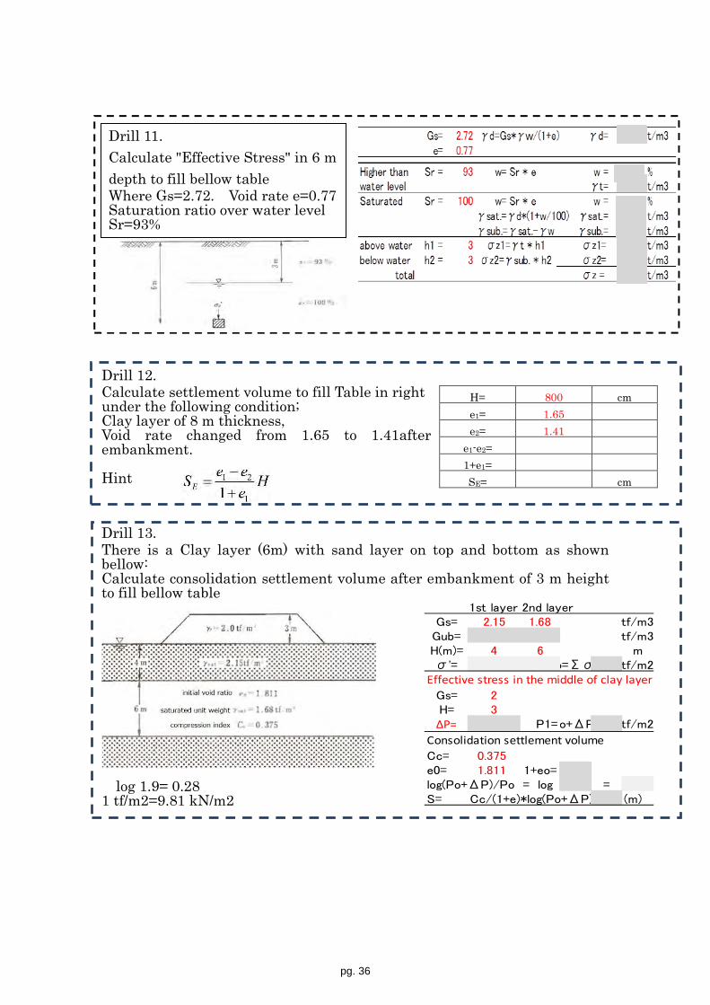
Drill 12. Calculate settlement volume to fill Table in right under the following condition; Clay layer of 8 m thickness, Void rate changed from 1.65 to 1.41after embankment. Hint Drill 13. There is a Clay layer (6m) with sand layer on top and bottom as shown bellow: Calculate consolidation settlement volume after embankment of 3 m height to fill bellow table

log 1.9= 0.28 1 tf/m2=9.81 kN/m2

H= 800 cm e1= 1.65 e2= 1.41

e1-e2= 0.24 1+e1= 2.65 SE= 72 cm

Drill 11. Calculate "Effective Stress" in 6 m depth to fill bellow table Where Gs=2.72. Void rate e=0.77 Saturation ratio over water level Sr=93%

1st layer 2nd layerGs= 2.15 1.68 tf/m3

Gub= 1.15 0.68 tf/m3H(m)= 4 6 mσ'= 4.6 2.04 o=Σσ6.64 tf/m2

Effective stress in the middle of clay layer Gs= 2H= 3

ΔP= 6 P1=o+ΔP12.6 tf/m2

Consolidation settlement volumeCc= 0.375e0= 1.811 1+eo= 2.81log(Po+ΔP)/Po = log 1.90 = 0.28S= Cc/(1+e)*log(Po+ΔP)0.22 (m)

pg. 37

Drill 14. Fill accumulated effective stress in bellow table after embankment for each clay layer (at the center of embankment) here, 3rd layer is sand layer, Ground water level is -3m. log 1.9= 0.281 tf/m2=9.81kN/m2

Drill 15. Calculate increased effective stress after embankment for each clay layer by using Osterverg chart. Then seek e0 and e1 from following figure and calculate the Consolidation Settlement. (Fill the blank sell of the following table)

For 1st Layer For2nd Layer

H (m) z (m) a/z b/z I ΣP1ΔP=I*ΣP1*2

ΣPoe0 fromFigure

e1 fromFigure

S Total S

53 1.5 6.7 3.3 0.49 126 123 261 3.5 2.9 1.4 0.48 155 148 55 0.88 0.81 0.044 6 1.7 0.8 0.46 174 160 74 0.88 0.81 0.15 0.19

1．Clayey Silt, trace Sand

2．Clayey Silt with fine Sand

CL

3m1m

γe =20KN/M3

γ1 =17KN/M3

γ2 =18KN/M3

5m

4m

b=5m

1:2

a=? m

1st layer2nd laye3rd laer FillH= 3 1 4 5

γt= 17 17 18 20γ'= 17 7 8 20

Weight= 51 7 32 100Po= 26 4 16 50

ΣPo= 55 74ΣP1= 126 155 174

H (m) γt γ' P0 ΣPo ΣP1

Fill 5 20 100

1st L. 3 17 26 26 126

2nd L. 1 17 7 4 55 155

3rd L. 4 18 8 16 74 174

pg. 38

5.4.3 Calculation of settlement time

Solution of consolidation theory has given the following relation.

Time coefficient: Tv =Cv/(H/2)^2*t

Consolidation ratio: U = S/Sf *100 (Here: S = Settlement, Sf = Final Settlement）

Estimation of Consolidation time

(1) Read each layer’s Cv value from the bellow “log Cv – log P” Graph.

Right Cv-P curve is for Kywe Chan Ye Kyaw Bridge approach road. From this graph read Cv value corresponding to the average action stress of targeted layers. In this case Cv – P graph is rather flat so we selected the value followings;

layer Cv value Remarks 1st layer 390 (cm2/ day) blue line 2nd layer 760 (cm2/ day) red line 3rd layer 1200 (cm2/ day) green line

Fig 36

Fig 37

pg. 39

(2) Then calculate an equivalent height of the Strata as a one layer.

Estimate S-t relation for actual consolidation layer by giving Cv: Consolidation coefficient the Equivalent Height, and Tv : Time coefficient.

Settlement – Time Relation (Unit; cm, Month)

This results shows it takes about 6 months for the 90% completion of “consolidation settlement”after finishing embankment of Kywe Chan Ye Kyaw Bridge approach road.

Right figure shows actual settlement observation record from April to November 2014.

Filling height became 1m at the end of May and during rainy season earthwork has been interrupted.

Consolidation settlement became 5 – 7cm due to this (1m high) filling and duration is around 3 months from beginning of embankment filling.

Calculation of Equivalent Height of StrataH0=H2*(Cv1/Cv2)^0.5+H3*(Cv1/Cv3)^0.5+H1

Cv HStrata 1 390 3.0Strata 2 760 1.5Strata 3 1200 1 H0= 5.83

t=(H/2)^2/Cv*TvH0= 583 Sf= 45 cmCv1= 390 t (day) Month

Tv( 100 ) 1.129 246 8.2 45.0Tv( 90 ) 0.848 185 6.2 40.5Tv( 80 ) 0.567 124 4.1 36.0Tv( 70 ) 0.403 88 2.9 31.5Tv( 60 ) 0.286 62 2.1 27.0Tv( 50 ) 0.197 43 1.4 22.5Tv( 40 ) 0.126 27 0.9 18.0Tv( 30 ) 0.071 15 0.5 13.5Tv( 20 ) 0.031 7 0.2 9.0Tv( 10 ) 0.008 2 0.1 4.5

St=Sf*Tv

Embankment Height (m)

Settlement (c m)

Fig 38

Fig 39

pg. 40

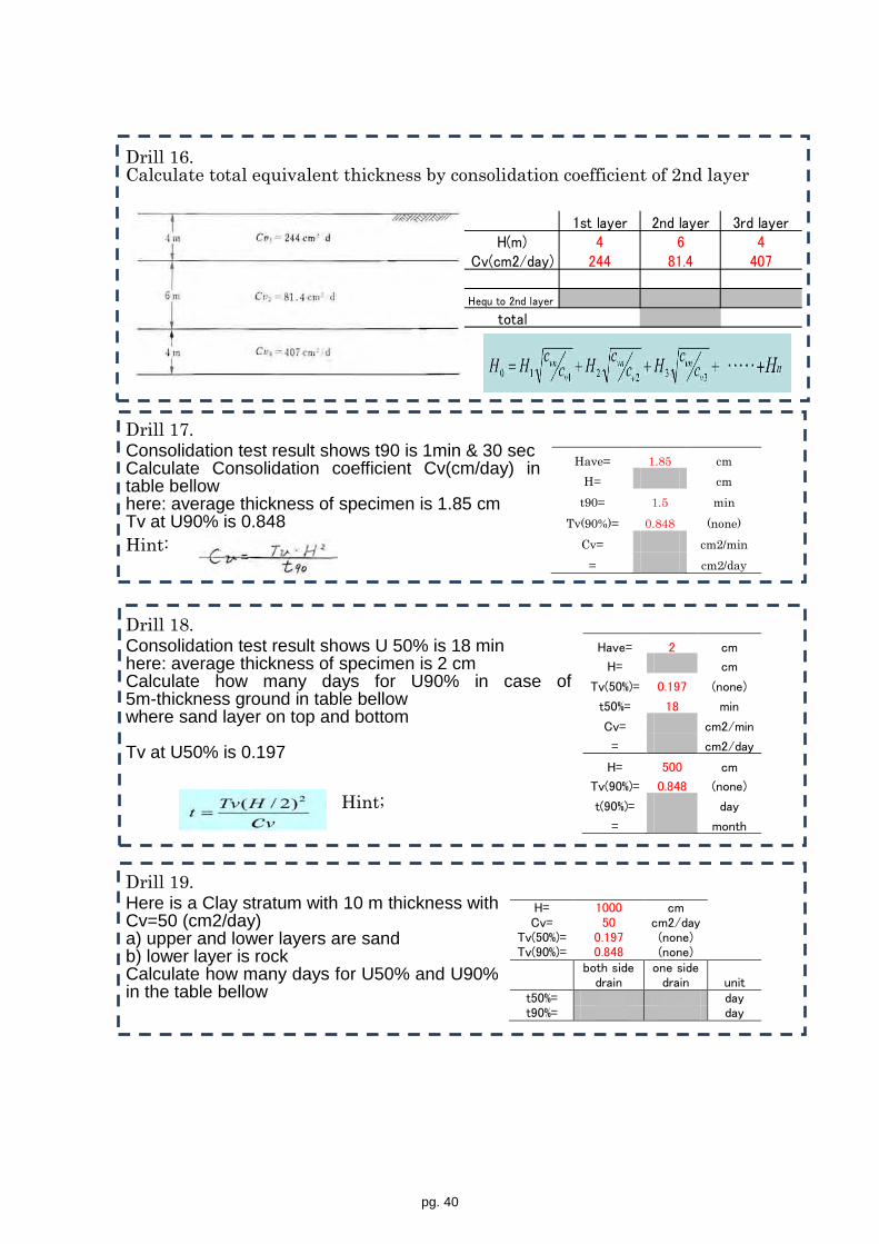
Drill 16. Calculate total equivalent thickness by consolidation coefficient of 2nd layer

Drill 17.Consolidation test result shows t90 is 1min & 30 secCalculate Consolidation coefficient Cv(cm/day) in table bellowhere: average thickness of specimen is 1.85 cmTv at U90% is 0.848 Hint: Drill 18. Consolidation test result shows U 50% is 18 minhere: average thickness of specimen is 2 cmCalculate how many days for U90% in case of 5m-thickness ground in table bellowwhere sand layer on top and bottom

Tv at U50% is 0.197

Hint; Drill 19. Here is a Clay stratum with 10 m thickness with Cv=50 (cm2/day)a) upper and lower layers are sandb) lower layer is rockCalculate how many days for U50% and U90%in the table bellow

Have= 1.85 cm H= 0.925 cm

t90= 1.5 minTv(90%)= 0.848 (none)

Cv= 0.484 cm2/min = 697 cm2/day

Have= 2 cm

H= 1 cm

Tv(50%)= 0.197 (none)

t50%= 18 min

Cv= 0.011 cm2/min

= 15.8 cm2/day

H= 500 cm

Tv(90%)= 0.848 (none)

t(90%)= 3363 day

= 112 month

H= 1000 cm Cv= 50 cm2/day Tv(50%)= 0.197 (none) Tv(90%)= 0.848 (none)

both side drain

one side drain unit

t50%= 985 3940 day t90%= 4240 16960 day

1st layer 2nd layer 3rd layerH(m) 4 6 4

Cv(cm2/day) 244 81.4 407

Hequ to 2nd layer 2.3 6.0 1.8total 10.1

pg. 41

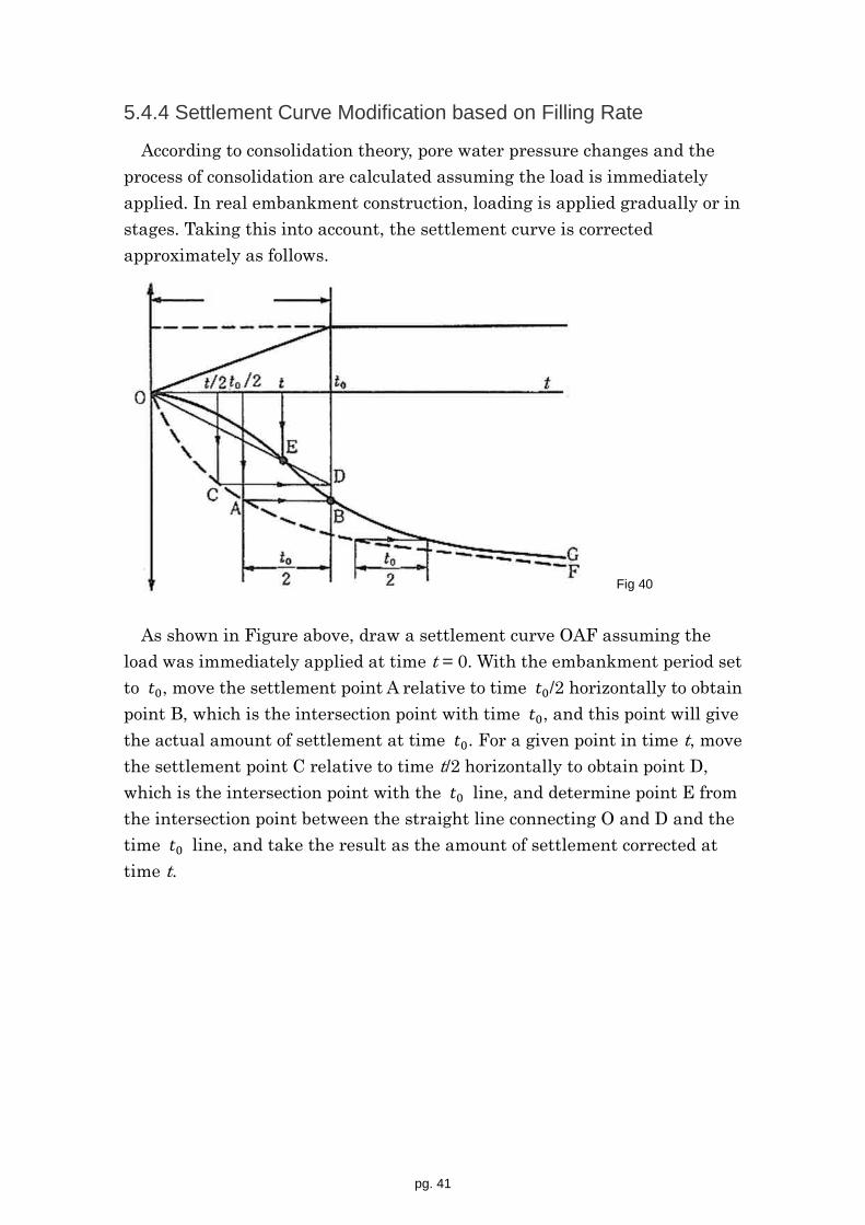
5.4.4 Settlement Curve Modification based on Filling Rate

According to consolidation theory, pore water pressure changes and the process of consolidation are calculated assuming the load is immediately applied. In real embankment construction, loading is applied gradually or in stages. Taking this into account, the settlement curve is corrected approximately as follows.

As shown in Figure above, draw a settlement curve OAF assuming the load was immediately applied at time t = 0. With the embankment period set to 𝑡0, move the settlement point A relative to time 𝑡0/2 horizontally to obtain point B, which is the intersection point with time 𝑡0, and this point will give the actual amount of settlement at time 𝑡0. For a given point in time t, move the settlement point C relative to time t/2 horizontally to obtain point D, which is the intersection point with the 𝑡0 line, and determine point E from the intersection point between the straight line connecting O and D and the time 𝑡0 line, and take the result as the amount of settlement corrected at time t.

Fig 40

pg. 42

5.4.5 Case study by Kywe Chan Ye Kyaw Bridge Project

Here is an example of settlement curve modification based on Filling work schedule as shown below. This figure made following assumptions;

The starting point of consolidation settlement is 7cm.

Construction period is 5months from Dec. 2014 to May 2015

This indicates consolidation settlement will finish November 2015.

Embankment Height (m)

Settlement (c m) Modified

Consolidation

Fig 41

pg. 43

6. Behavior Observation during Construction

One of the objects of Technical Cooperation Project for “Improvement of Road Technology in Disaster-affected Areas in Myanmar” (TCP) is the technical transfer of the treatment of high embankment. However, construction works in Ayeyarwady delta area has been conducting under the tight schedule and budget. And newly adoption of countermeasure works is not practical.

Therefore, TCP team has proposed to carry out “Observation works” and “Analysis works” of the behavior of high embankment by installing necessary apparatus on starting the embankment work.

Here, we introduce a method of field observation conducted at Kywe Chan Ye Kyaw Bridge approach slope embankment.

Necessity reason of the observation 1) Soil investigation survey could not always obtain enough data for

designing 2) Comparison with Analysis results and observation results

Fig 42 Flow Chart of Observation of embankment behavior

1 Making Observation Plan

Outline of the targeted Construction

Measurement items and method of

observation

2

Preparation of Field Observation of Embankment Behavior

Arrangement of Observation Instrument

Procurement of the Instrument Setting of Instrument

3

Observation Measurement and Record

Observation, Measurement and recording

Data processing and analysis Feed back to Construction works

4 Reporting

Record of Construction Progress Record of data analysis

Proposal for future Construction

works

pg. 44

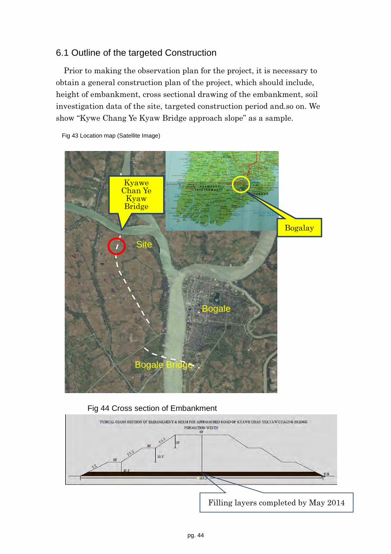
6.1 Outline of the targeted Construction

Prior to making the observation plan for the project, it is necessary to obtain a general construction plan of the project, which should include, height of embankment, cross sectional drawing of the embankment, soil investigation data of the site, targeted construction period and.so on. We show “Kywe Chang Ye Kyaw Bridge approach slope” as a sample.

Fig 43 Location map (Satellite Image)

Fig 44 Cross section of Embankment

Filling layers completed by May 2014

Bogale

Bogale Bridge

Kyawe Chan Ye

Kyaw Bridge

Bogalay

Site

pg. 45

Fig 45 Plan and Profile of embankment adjacent to the Abutment

Bogale side

pg. 46

Cross section of the Embankment at the highest point

Dimension of Embankment work Measurement Unit in feet Unit in meter

Existing 98 29.9 Finished 126 38.4 Embankment height 28 8.5 Embankment Length 1,600 487.7 Longitudinal slope 2.5% (average) Embankment top width 40 12.2 Embankment bottom width (at highest section)

182 55.5

Volume of approach road embankment (Total) 76,465m3

Construction Schedule (Earth work) is shown in Annex 1

H

8.48.28.07.87.67.4

24.30

7.2

5.6

24.60

24.00

L8.6

23.7023.4023.1022.8022.50

3.2 m

3.2 m

h = (H-6.2) m

6.4m 6.1 m4.8 m 3.0 2.0 m2.0 m

Cross Section of Embankment(at the highest )

L= (H-6.4)x 1.5+6.1 + (2+4.8+2+6.2)

Fig 46

pg. 47

6.2 Outline of Observation methods

Instrumentation and monitoring on soft ground is meant to provide additional information obtained in the construction process to compensate for uncertain factors and to reliably complete the embankment work. Measurement devices are arranged, ground monitoring is conducted for settlement management or stability management, the obtained measurement information is evaluated, and this is fed back to the next work process. The operational flow of instrumentation and monitoring is shown in below.

Fig 47 Work control with soft ground monitoring

*1 waiting time for embankment, reduce filling rate and so on.

Surcharge, etc.Design

Execution of treatment work as required

Instrumentation, etc.

Ground monitoring Construction of earthwork structure Ground

monitoring

Settlement managemen

Countermeasure*1

Stability managemen

Continuation of bankingFilling rate increase

Countermeasure*1

Completion

OK OK

NG NG

Investigation

pg. 48

6.3 Measurement method of observation and necessary instruments

Measurement items and method of observation No. Measurement item (Purpose) Methods

1Movement of embankment for three dimensional direction

Observation of stakes set on the embankment and its beside area

2Settlement of the ground under the embankment

Install settlement board

3 Movement of under-ground by inclinometerChecking the inclination of vertical pipe by inclinometer

4 Changing of pore-water pressure in the ground Pore-water pressure gauge5 Under ground water level Installing an observation well.

Necessary number of instruments Observation Item Equipment Number

1Surface

MovementPegs and 18 pointTotal station 1 No.

2. Settlement Settlement Plate 4 point

3. Under Ground MovementInclinometers & 1 Noguide pipe 4 point

4. Pore-Water Pressure Pore-water pressure gauge 3 point

5 Ground water levelWater level meter 1 NoObservation well 1 point

Embankment

Settlement Plate

Pore water pressure

gauge

Surface deformation

peg

Inclinometer underground

movement

Soft ground

These are most important are most

Fig 48

pg. 49

Detail of instruments for measurement is shown in bellow.

Following apparatus are not installed but used on the time to measure

Sensor is dropped down into the PVC pipe. Water level is informed by buzzer and red indicatorsTotal weight is 18 kg with 50m-length cable.

Inclinometer Water level gauge

Total station for 3-D survey Data logger for measuring data

Settlement Plate Pore Pressure gauge

Inclinometers are inserted into special guide pipes to measure inclination.

Fig 49

pg. 50

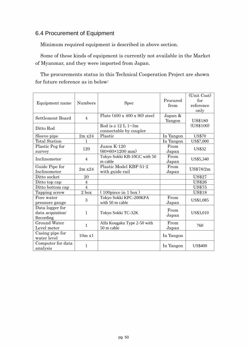
6.4 Procurement of Equipment

Minimum required equipment is described in above section.

Some of these kinds of equipment is currently not available in the Market of Myanmar, and they were imported from Japan.

The procurements status in this Technical Cooperation Project are shown for future reference as in below:

Equipment name Numbers Spec Procured from

(Unit Cost) for

reference only

Settlement Board 4 Plate (400 x 400 x 90) steel

Japan & Yangon US$180

(US$100) Ditto Rod Rod isφ12 L 1~3m connectable by coupler

Sleeve pipe 2m x24 Plastic In Yangon US$70 Total Station 1 In Yangon US$7,000 Plastic Peg for survey 120 Juzen K-120

(60×60×1200 mm) From Japan US$32

Inclinometer 4 Tokyo Sokki KB-10GC with 50 m cable

From Japan US$5,340

Guide Pipe for Inclinometer 2m x24 Plastic Model KBF-51-2

with guide rail From Japan US$78/2m

Ditto socket 20 US$27 Ditto top cap 4 US$26 Ditto bottom cap 4 US$75 Tapping screw 2 box ( 100piece in 1 box ) US$18 Pore water pressure gauge 3 Tokyo Sokki KPC-200KPA

with 50 m cable From Japan US$1,085

Data logger for data acquisition/ Recording

1 Tokyo Sokki TC-32K From Japan US$3,010

Ground Water Level meter 1 Alfa Kougaku Type 2-50 with

50 m cable From Japan 760

Casing pipe for water level 10m x1 In Yangon Computer for data analysis 1 In Yangon US$400

pg. 51

6.5 Arrangement plan of observation Instrument

Three sectional observation line of instruments are set along the centerline of embankment with distance of 50m each. Instrument Arrangement plan is shown below:

Fig 50

pg. 52

6.7 Setting of instrument

Each measurement instrument is installed before embankment earth work start in the holes drilled by boring machine.

6.7.1 Settlement Plate:

Installation of Settlement Plate is done by following steps: 1) Clear the setting position on embankment

surface and compact well. 2) Shape the position to a flat and level. 3) Place a Settlement plate with level and attach

Rod with PVC Isolation pipe cover. 4) Fill and compact carefully surrounding not to

move or damage the settlement plate. 5) Filling work of surrounding are (around 50cm

radius) shall be done manually by using a small compaction plate.

6) According to the progress of embankment, add extension Rod joining by special nut. Also extend Isolation PVC pipe by socket at a same time.

7) Whenever join new Rod, the top elevation should be measured and recorded. (see Chapter 8: data recording Form sheet)

6.7.2 Pour water pressure measurement device

Device is set at a bottom of the borehole placed at the center of road embankment by following step: 1) Install a Pore water pressure gauge inside

of the borehole. And fill the surroundings of cable by sand up to around 50cm height. (on refilling method)

2) Then put soil cement around 50cm height and Cement milk 50cm height to isolate the pore pressure of measurement point.

3) The top of boring hole should be covered by soil (H=30 cm), and area of 0.5m from center of boring should be compacted manually.

4) Lead Cable should be buried within a

Fig 51

Fig 52

pg. 53

narrow ditch around 20cm depth. 5) Protect the cable end inside of waterproof box.

6.7.3 Inclinometer guide pipe

Install guide pip in a borehole. Setting of guide pipe pprocedure is following. 1) Bore the hole 10m depth then insert guide pipe inside of Borehole.2) On inserting guide pipe in the borehole, one pair of the shallow guide (slit) direction

of the pipe should be perpendicular to the road embankment centerline. (Important!)

3) Join guide pipe using socket and tapping screw. Each length should be 2m x 4 = 8m.

4) After inserted the guide pipe, space between bore hole and guide pipe should be filled by fine sand.

5) The top of the guide pipe should be 50 cm heightfrom ground and be protected by some frame as shown in right.

6.7.4 Water level measurement well

PVC pipe with a strainer will be installed for measurement of water level by measurement instrument.

Setting of PVC pipe procedure is following: 1) After survey of embankment area setting location

should be marked. The location should be well considered the flood season also easy to access for observation.

2) Bore the hole 10m length then insert PVC pipe inside of Bore hole. Before insert, PVC pipes are made strainer covered with nonwoven fabric to prevent sand into the well.

3) The top of the PVC pipe should be 50 cm height from ground and be protected by some frame.

4) After inserted the PVC pipe, space between bore hole and PVC pipe should be filled by fine sand.

z

L=1.0m

L=7.0 m Strainer section: Short strip cut with saw or drilled holes

H=30cm

H=30cm

L=7.5 m Cover by fabric to protect from sand entering inside of well

Fig 53

Fig 54

pg. 54

6.7.5 Peg for deformation survey

To measure the deformation of embankment and surrounding, stakes are installed in the ground as a mark for measure the deformation by Total station.

For easy to distinguish the many observation points and results, systematic numbering (naming) of the point is recommended.

Example; Observation Pont of Numbering for Kywe Chan Ye Kyaw bridge, approach slope

Refer Drawing of Chapter 6.5

Observation Point NumberingPeg for Survey

Inc linomater

Pore Water Pressure

Settelment Plate

Well for Water level

IL1IL2

IR1IR2

SR1PC1SR2 PC2PC3

Slope Toe

Slope Toe

Center e Line

SL2 SL1

OL12

OL11

OL13

OR11

OR12

OR13OR23

OR22

OR31

OR32

OR33

OL31

OL32

OL33

OL21

OL22

OL23

River Side ⇒OR21

⇐Bogale SideSlope Sholuder

Slope Sholuder

Fig 55

pg. 55

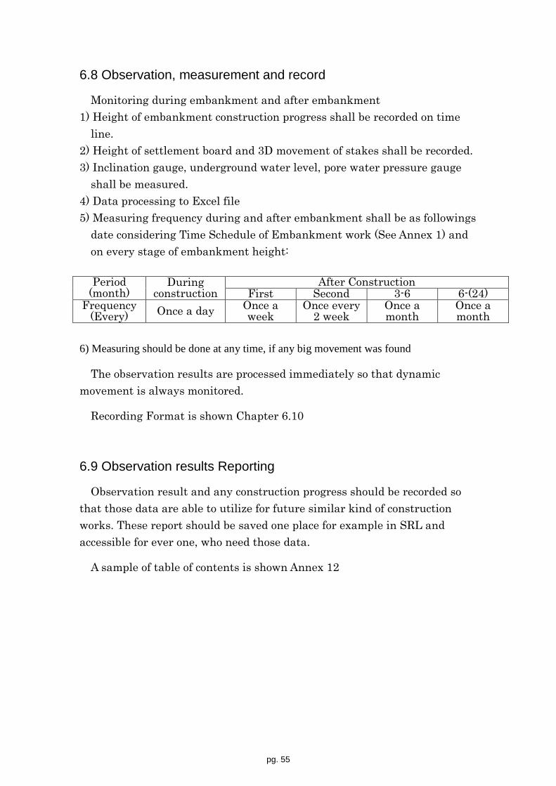
6.8 Observation, measurement and record

Monitoring during embankment and after embankment 1) Height of embankment construction progress shall be recorded on time

line. 2) Height of settlement board and 3D movement of stakes shall be recorded. 3) Inclination gauge, underground water level, pore water pressure gauge

shall be measured. 4) Data processing to Excel file 5) Measuring frequency during and after embankment shall be as followings

date considering Time Schedule of Embankment work (See Annex 1) and on every stage of embankment height:

Period

(month) During

construction After Construction

First Second 3-6 6-(24) Frequency

(Every) Once a day Once a week

Once every 2 week

Once a month

Once a month

6) Measuring should be done at any time, if any big movement was found

The observation results are processed immediately so that dynamic movement is always monitored.

Recording Format is shown Chapter 6.10

6.9 Observation results Reporting

Observation result and any construction progress should be recorded so that those data are able to utilize for future similar kind of construction works. These report should be saved one place for example in SRL and accessible for ever one, who need those data.

A sample of table of contents is shown Annex 12

pg. 56

6.10 Example of the data processing of Measurement results

The observation results are processed immediately means visualize the obtained data and make it easy to find any trend of measurements result.

6.10.1. 3-D measurement

3-D measurement by Total Station is rather complicated. And we should well consider the proper Turning point location, which could see through both side of road embankment stakes throughout the construction.

3-D measurement data are recorded on a following form;

Date TS Target N E Z HI HP GL

2014/11/21

BM0 4000 2000 10

BM1 3965.978 1888.713 10.284

BM1 BM0

TP1 3923.114 1913.962 9.817

TP1 MB1

OR11

OR12 3941.854 1854.753 9.732

OR13 3934.258 1861.055 9.583

OR21

OR22 3914.759 1815.071 9.603

OR23 3906.935 1821.14 9.375

OR31

OR32 3889.998 1771.504 9.566

OR33 3881.495 1776.773 9.567

BM1 TP1

TP2 4021.627 1866.196 10.095

TP2 BM11

BM12 3985.685 1817.803 9.854

BM13 3993.387 1811.554 10.007

BM21

BM22 3955.981 1783.263 9.809

BM23 3963.669 1776.807 10.002

BM31

BM32 3927.891 1744.225 10.506

BM33 3935.799 1737.541 9.815

BM1 TP2

BM0

pg. 57

The movement of the targeted stake head is calculated from the comparison of survey data of the difference date of each points coordinate (N,E,Z)

Surveyor tried 3 times of measurement up to Nov 2014, but the each measured results is not within a satisfactory error limits.

6.10.2 Settlement Plate

Each Settlement Plate’s observation data are recorded on following form:

Date Filled Elevation

Filled total Height

Top level of rod

Rod Length

Settlement Plate

bottom Elevation

Accumulated settlement

(m) (m) (m) (m) (m) (cm)

Initial 29.9 0.00 (31.9) 28.080 SB1R

2014/4/30 0.15 29.900 1.825 28.075 0.0

2014/5/8 0.45 29.894 1.825 28.069 -0.6

2014/5/15 0.59 29.886 1.825 28.061 -1.4

2014/5/30 31.15 1.15 29.865 1.825 28.040 -3.5

2014/6/15 1.13 29.851 1.825 28.026 -4.9

2014/7/15 1.11 29.831 1.825 28.006 -6.9

2014/9/30 1.10 29.827 1.825 28.002 -7.3

2014/11/11 1.10 29.827 1.825 28.002 -7.3

2014/12/12

29.826 1.825 28.001 -7.4

2015/1/? 3.650

Then measured data are plotted to following graph with embankment height and settlement.

pg. 58

6.10.3 Inclinometer

Inclinometer observation data are recorded on a following form:

layer 1 layer 2IL1 2014/5/8 IL1 2014/5/18Depth X+ X- X+ - X- / 2 Section Accum. Depth X+ X- X+ - X- / Section Accum.

0.50 -250 345 -298 0.25 0.10 0.50 -234 331 -283 0.86 1.86 1.00 -225 326 -276 -0.06 -0.14 1.00 -210 308 -259 0.61 1.00 1.50 -196 302 -249 -0.06 -0.08 1.50 -188 290 -239 0.35 0.39 2.00 -128 233 -181 -0.02 -0.02 2.00 -129 229 -179 0.04 0.04 2.50 -56 161 -109 -0.04 0.00 2.50 -57 157 -107 0.02 0.00 3.00 -17 119 -68 -0.08 0.04 3.00 -19 121 -70 -0.16 -0.02 3.50 21 82 -31 0.02 0.12 3.50 19 81 -31 0.00 0.14 4.00 96 5 46 -0.08 0.10 4.00 93 8 43 -0.20 0.14 4.50 135 -32 84 -0.08 0.18 4.50 133 -33 83 -0.10 0.35 5.00 127 -25 76 0.06 0.27 5.00 125 -26 76 0.04 0.45 5.50 104 0 52 0.06 0.20 5.50 104 -2 53 0.10 0.41 6.00 74 26 24 -0.04 0.14 6.00 74 22 26 0.04 0.31 6.50 63 40 12 -0.04 0.18 6.50 61 38 12 -0.04 0.27 7.00 75 29 23 -0.02 0.23 7.00 73 26 24 0.00 0.31 7.50 75 27 24 0.00 0.25 7.50 72 27 23 -0.06 0.31 8.00 10 89 -40 0.12 0.25 8.00 12 85 -37 0.25 0.37 8.50 -69 174 -122 0.04 0.12 8.50 -70 171 -121 0.08 0.12 9.00 -70 173 -122 0.02 0.08 9.00 -70 171 -121 0.06 0.04 9.50 -76 180 -128 0.06 0.06 9.50 -77 177 -127 0.10 -0.02

10.00 -41 145 -93 0.00 0.00 10.00 -43 149 -96 -0.12 -0.12 10.50 26 77 -26 -0.02 0.00 10.50 24 75 -26 -0.02 0.00

Input yellow colored cells only, the other cells are automatically calculated and filled and the Chart is also automatically drawn.

To extend a new Data box select whole area and copy it and paste to another area.

To plot new data on a graph:

Put a cursor on a graph plotting area and click a right button of mouse ⇒

Graph tool, design menu appear. Chose a Select data menu. Then a “Select Data Source dialog” will appear. Here, you can change the data source.

Fig 56

pg. 59

Select same type of data then, click the “Add” Enter the area of “Series Name”, “X value”, “Y value” by selecting each cell area, which include new value.

6.10.4 Pore pressure meter

Pore Pressure 1

Calibrationfactor = 1) 0.106

Date Time Reading PP 12014/3/26 1550 617 64.792014/4/8 1440 651 68.362014/4/30 1130 717 75.292014/5/8 800 719 75.502014/5/18 1030 743 78.022014/5/30 1300 751 78.862014/6/15 1500 773 81.172014/7/15 1000 773 81.172014/9/30 1300 778 81.692014/11/11 1500 793 83.27

1) Calibration factor should be written from “Pore pressure transducer test data”, which is attached each instrument.

The graph is also plotted same way as described as “The Inclinometer” section.

Fig 57

Fig 58

Fig 59

pg. 60

6.10.5 Underground Water level Record the measured data (depth from well head) on the following form. Elevation of well head is also necessary to be measured by level survey once a while.

Elevation of Well head = 20.00

Date Time Measured Water Level 2014/4/8 1440 1.27 18.732014/4/30 1130 0.97 19.032014/5/8 800 0.99 19.012014/5/18 1030 0.80 19.202014/5/30 1300 0.67 19.33

Fig 60

pg. 61

6.11 Analysis of obtained data & usage

Following are Examples of the observation data analysis Instrument Flow of the

processing Example of result

Settlement Plate

(Settlement of the base of embankment)

Survey record of

Total station or

Level

measurement

→(Data transfer

to Excel file)

Time – Settlement Relation with the progress of

embankment

Observation Points

(settlements the ground surface around embankment)

Survey record of

Total station

→(Data transfer

to Excel file)

Time – Settlement Relation with the progress of

embankment

Inclinometer

(Lateral movement of the ground around embankment)

Data Logger

→ (cable)

→ PC

Chart of Lateral movement – Depth

Fig 61

pg. 62

Qualitative trend of unstable conditions 1) Occurring small crack on

surface of embankment. 2) Rapid increase of settlement

in a center. 3) Rapid increase of horizontal

deformation to outside. 4) Rapid increase of vertical

deformation to upward. 5) Continuous increase of

deformation and pore water pressure even after stopping banking.

Fig 62

pg. 63

7. Study about Countermeasure

7.1 Countermeasure study at each stage

Countermeasures should be studied at each stage as shown bellow:

Notice on Design stage * It is important to check a level of countermeasure in outline design. * Design of stability and settlement countermeasure according with the

level.

Required items on Analysis * Understanding of situation of ground based on ground investigation. * Analysis of stability and settlement. * Prediction of stability and settlement by observational method.

7.2 Necessary countermeasure study for Stability during construction

If a sign of ground failure is found, sufficient checks are required prior to taking corrective actions, and the communication process in the event of an emergency must be thoroughly carried out. If the values exceed the control levels, the works is immediately suspended, ground monitoring is continued, and attention is paid to subsequent ground actions. If the instability continues even after the suspension of works, appropriate actions are taken including the immediate removal of part of the fill. Furthermore, soil

Observation and prediction Stability Settlement

Detail investigation and analysis Calculation of stability and settlement

Outline of ground investigation Understanding of situation of ground An

alys

is

Construction Embankment with Countermeasure

Detail design Design of countermeasure Method (Stability and settlement)

Outline of design Check of level of countermeasure method Proposal of several designs

Des

ign

Feed back

Fig 63

pg. 64

investigations are conducted and a detailed study (e.g., stability calculation) is made based on the newly acquired ground strength data.

Even if the changes are within the control levels, when actions occur that are close to the limit, it is recommendable to execute the works carefully (e.g., by reducing the filling rate as required). When the filling rate is controlled during execution of the slow loading method, for example, and sufficient stability is confirmed by ground monitoring, appropriate response actions are taken, including increasing the filling rate, while monitoring the conditions.

7.3 Necessary countermeasure for settlement work

If the settlement ascertained from the results of ground monitoring is different from the predicted value, the following points are studied depending on the amount of the difference. a) The earthwork volume and workmanship (slope and top width) of the

embankment. b) The amount of preloading, the period of loading, when the surcharge

method is used. And study to remove the extra banking from the settlement data.

c) When to construct a structure that is to be constructed after removing the extra banking, the amount of settlement should be estimated that would continuously occur even after execution, and should determine the amount of extra banking are decided.

d) The amount of uneven settlement should be calculated at the boundary between a structure supported by piles and an embankment directly applied on the soft ground, whether uneven settlement after the completion of banking would harm the structure itself, and measures should be studied (e.g., approach slabs).

7.4 List of Countermeasures to be taken in general

Following table shows countermeasures to reduce settlement and to increase Safety Factor (Sf).

pg. 65

Table: Applicability of Countermeasures for Settlement and Stability

Theory Typical methods

Settlement Stability Deform

Secu

ring

of T

raffi

cabi

lity

Appl

icab

ility

in M

yanm

ar

Acce

lera

tion

of

cons

olid

atio

n se

ttle

men

t Re

duci

ng o

f t

otal

set

tlem

ent

Incr

easi

ng o

f str

engt

h

by co

nsol

idat

ion

Incr

easi

ng o

f

Resi

stan

ce fo

r slid

ing

Redu

cing

of

Sl

idin

g fo

rce

Isol

atio

n of

str

ess

Redu

cing

of s

tres

s

Consolidation & drainage

Drain of Surface water ○ ○ Sand mat ○ ○ ○ Slow banking method ○ △ Surcharge ○ ○ △ Vertical drain

Sand drain ○ ○ Pre-fabricated drain ○ ○

Vacuum Consolidation ○ ○ Ground water level reduction ○ ○ △

Compaction Vibratory compaction

Sand pile ○ ○ ○ ○ ○ Rod compaction ○ Vibro-floatation ○ Vibro-tamper ○

Static compacted sand pile ○ ○ ○ ○ ○

Solidification

Shallow soil stabilization ○ ○ ○ ○ ○

Deep mix Mechanical mix ○ ○ ○ ○ Jet grouting ○ ○ ○ ○

Lime pile ○ ○ Chemical grouting ○ ○ Freezing ○

Excavation & replacement ○ ○ ○ △

Load reduction

Embankment by Light Weight materials/soil

Styrofoam block ○ ○ ○ Bubble-mix soil ○ ○ ○ Formed bead-mixed soil ○ ○ ○

Culvert ○ ○ ○ △ Embankment Reinforcement ○ ○ Structural Counterweight filling ○ ○ Counter-measure Sheet pile ○ ○ Laying of reinforced materials (Ex. Geo-textile) ○ ○ △

From above various counter measure, here we show two most common method.

pg. 66

7.4.1 Preloading method:(Surcharge method, Extra banking method)

As a counter measure most easy and reliable way is a surcharge methods include constructing an embankment in advance to accelerate consolidation. If the construction period is sufficiently long, residual settlement can be reduced by using a slow banking method, which involves spending a long time to construct an embankment.

Embankmentperiod

Waiting period

Removal of load

Construction of structure + embankment

Pavement

LoadP

SettlementS

SurchargeProposedload Pf

Time

Residual settlement𝛥S

Final settlement

(a) Surcharge method (between structures)

Embankment height HE

Settlement

S

Extra banking

Embankmentperiod

Waiting period

Removal of load

Pavement

Opening to services

Opening to services

Proposedembankment height HEf

Time

Residual settlement𝛥S

Final settlement

Final settlement including extra fill

(b) Extra banking method (ordinary embankment section)

Fig 64

pg. 67

7.4.2 Vertical drainage construction method (Sand Pile)

One of the most effective way to shorten the period of “consolidation settlement” is the vertical drain method, in which drain materials are installed in the vertical direction in the soft soil layer at appropriate intervals to reduce the consolidation drainage distance in the lateral direction in order to accelerate consolidation.

Fig 65 Layout of sand drains and status of consolidation drainage

Fig 66 Vibro-hammer type sand drain method execution procedure

Embankment loadSand mat

Sand

dra

in

(a) Regular triangle layout (b) Square layout Groundwater flow

(Positioning)

Mobilization Penetration

(Completion of penetration)

Construction of sand piles

(Completion of construction)

Vibrator

Sand

Bottomendtrack

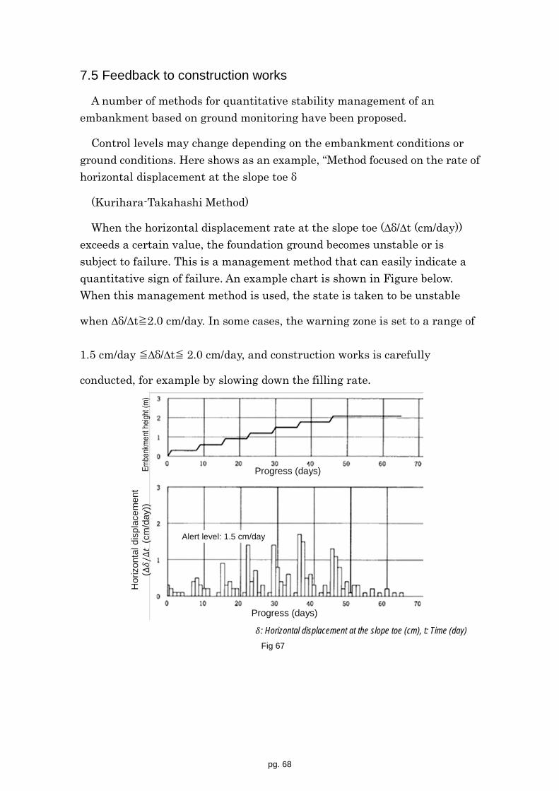
pg. 68

7.5 Feedback to construction works

A number of methods for quantitative stability management of an embankment based on ground monitoring have been proposed.

Control levels may change depending on the embankment conditions or ground conditions. Here shows as an example, “Method focused on the rate of horizontal displacement at the slope toe δ

(Kurihara-Takahashi Method)

When the horizontal displacement rate at the slope toe (∆δ/∆t (cm/day)) exceeds a certain value, the foundation ground becomes unstable or is subject to failure. This is a management method that can easily indicate a quantitative sign of failure. An example chart is shown in Figure below. When this management method is used, the state is taken to be unstable

when ∆δ/∆t≧2.0 cm/day. In some cases, the warning zone is set to a range of

1.5 cm/day ≦∆δ/∆t≦ 2.0 cm/day, and construction works is carefully

conducted, for example by slowing down the filling rate.

𝛿: Horizontal displacement at the slope toe (cm), t: Time (day)

Emba

nkme

nt he

ight (

m)

Progress (days)

Hor

izon

tal d

ispl

acem

ent

(∆𝛿/∆𝑡

(cm

/day

))

Alert level: 1.5 cm/day

Progress (days)

Fig 67

pg. 69

Fig 68 Countermeasure for bridge abutment back face

Embankment

Fig 69

Fig 70

pg. 70

Surcharge or pre-loading method Fig 71

Annex

Annex 1 Brief explanation about using of Geostudio Annex 2 Inquiry about further information of GeoStudio Annex 3 Formula used in Excel sheet Annex 4: Excel method modified “C” to maximum 5 layers. Annex 5: Organized way of consolidation test results Annex 6: Consolidation Curve plotting and yield point on e-log P curve Annex 7: Plotting of log Mv-log P curve Annex 8: Sample of obtaining e-log p curve by MS Excel Annex 9: Sample of obtaining Cv and log Cv – log P curve by MS Excel Annex 10: JIS Data Format Sheets Annex 11. Schedule of Approach embankment with Observation Plan Annex 12. Sample of Table contents for Observation analysis result report Annex 13 (sample) Specification of Embankment at Approach Road to Bridges Annex 14: Answer of Drills

A1-1

Annex 1 Brief explanation about using of Geostudio

Simple manual for usage of Geo Studio Slope/W 1. Select: Student License 2. Click SLOPE/W

3. Come out following display. Ignore and Click “CLOSE” (right side of

bottom)

A1-2

4. Select from Draw (Pull down Menu) Points and input necessary points It is better to prepare following X-Y table in advance referring Fig 6

Shoulder

0,20.3 6.1,20.3 Berm 2

11.4,16.8 14.4,16.8 Berm 1

19.4,13.4 22.4, 13.4 Toe

0.10 29.1, 10

1st layer 0,7 29.1, 7 50,10

2nd layer 0,5.5 50,5.5

3rd layer 0,4.5 50,4.5

Note: Y is modified by adding 10 in order to adjust the location of cross section At first, locate each point by integral number (m)

5. Click Point number button, then each points have its point number

Then, Select from KeyIn (Pull down Menu) Points and input detailed number

A1-3

6. Select from Draw (Pull down Menu) Regions. Repeat about 3 regions

Note: maximum material number is 3 in case of Student version

A1-4

7. Select from Keyin (Pull down Menu) Materials. Add button-> New-> Input Name. Select Material Model Mohr-Coulomb. And add data

8. Select Draw Material Button and Click applicable region, then the region has color

Coulomb. And add data> New-

Coulomb. And add dataInput Name. Select Material Model MohrInput Name. Select Material Model Mohr

A1-5

9. Select from Draw (Pull down Menu) Slip surface→Entry & Exit, then click Done

10. Select and Click Analysis Name from Solve Manage window and Click start

11.You are requested to input File Name and location to be saved 12. Click Start and you will get Stability Analysis results as follow:

A2-1

Annex 2 Inquiry about further information of GeoStudio

Ask for geo slope training by Google (Inter-net)

Select: Workshop Movies - GEO-SLOPE International Ltd.

There are 3 items useful for understanding Tips & Tricks

General Tips and Tricks Page size and drawing scale (16:55) Import DXF data (14:39) Import Pictures (20:06) Modify Objects (8:13) Dynamic Sketch Text (18:00) Viewing Objects and Results (5:29) Microsoft Office Integration (5:13) Reporting (2:45) Input and Output Files (3:31) Product Tutorials

See --- Movie “Getting Started with SLOPE/W 2007” (separate attachment) Slope/W

SLOPE/W Session 1 Introduction and Fundamentals (52:09) Geometry (42:42) Material Properties (46:03) Trial Slip Surfaces (1:06:21) Pore Pressures (31:26)

SLOPE/W Session 2 Introduction to Reinforcements (40:22) Anchors (37:10) Nails (20:24) Geofabric (19:04) Piles and Dowels (8:00) Seismic (16:47) Probabilistic (21:42)

http://www.geo-slope.com/support/workshop/

http://www.geo-slope.com/support/workshop/general.aspx?id=wshpgeostudiosetscale

http://www.geo-slope.com/support/workshop/general.aspx?id=wshpgeostudioimportdxf

http://www.geo-slope.com/support/workshop/general.aspx?id=wshpgeostudioimportpicture

http://www.geo-slope.com/support/workshop/general.aspx?id=wshpgeostudiomodifyobjects

http://www.geo-slope.com/support/workshop/general.aspx?id=wshpgeostudiodynamicsketchtext

http://www.geo-slope.com/support/workshop/general.aspx?id=wshpgeostudioviewdetails

http://www.geo-slope.com/support/workshop/general.aspx?id=wshpgeostudiomicrosoftintegration

http://www.geo-slope.com/support/workshop/general.aspx?id=wshpgeostudioreporting

http://www.geo-slope.com/support/workshop/general.aspx?id=wshpgeostudioinputoutputfiles

http://www.geo-slope.com/support/workshop/products/slope.aspx?id=wshpslopefundamentals

http://www.geo-slope.com/support/workshop/products/slope.aspx?id=wshpslopegeometry

http://www.geo-slope.com/support/workshop/products/slope.aspx?id=wshpslopematerials

http://www.geo-slope.com/support/workshop/products/slope.aspx?id=wshpslopetrialslips

http://www.geo-slope.com/support/workshop/products/slope.aspx?id=wshpslopeporepressure

http://www.geo-slope.com/support/workshop/products/slope.aspx?id=wshpslopereinforcementintro

http://www.geo-slope.com/support/workshop/products/slope.aspx?id=wshpslopeanchors

http://www.geo-slope.com/support/workshop/products/slope.aspx?id=wshpslopenails

http://www.geo-slope.com/support/workshop/products/slope.aspx?id=wshpslopegeofabric

http://www.geo-slope.com/support/workshop/products/slope.aspx?id=wshpslopereinforcementgeneral

http://www.geo-slope.com/support/workshop/products/slope.aspx?id=wshpslopeseismic

http://www.geo-slope.com/support/workshop/products/slope.aspx?id=wshpslopeprobabilistic

A3-1

Annex 3 Formula used in Excel sheet N13: Left X = IF(G14>0,"",F6-((R0^2-(F7-F4)^2))^0.5) N14: Left Y= F4 R13: Right X = +F6+((F8^2-(F3-F7)^2))^0.5, R14: Right Y= F3 P13: shoulder X = F$5*P14, P14: shoulder Y= F3 O13: m1 X = (-b-(b^2-4*a*Cc)^0.5)/(2*a) O14: m1Y= IF(O13="","",O13/n) Q13: m2X = (-b+(b^2-4*a*Cc)^0.5)/(2*a) Q14: m2Y= Q13/n Here a= 1+1/(n^2), b= -2*(X0+Y0/n), c= =X0^2+Y0^2-R^2 F12: left end X = MIN(N13:O13), G12: left end Y = -((F$8^2-(F12-F$6)^2)^0.5)+F$7 F13: right end X = (R0^2-(G13-F7)^2)^0.5+F6, G13: right end Y= MIN(Q14:R14) F17: X circle =F12+F$10/2, F18: X circle =IF(E18>F$9,"",F17+F$10), F19: X circle = IF(E19>F$9,"",F18+F$10) --------- --------- G17: Y circle = -((F$8^2-(F17-F$6)^2)^0.5)+F$7 G18: Y circle = IF(E18>F$9,"",-((F$8^2-(F18-F$6)^2)^0.5)+F$7) G19: Y circle = IF(E19>F$9,"",-((F$8^2-(F19-F$6)^2)^0.5)+F$7) --------- --------- H17: Y topline =IF(F17="","",IF(F17>P$13,F$3,IF(E17>=F$9,F$3," "))) H18: Y topline =IF(F18="","",IF(F18>P$13,F$3,IF(E18>=F$9,F$3," "))) ------- I17:Y slope =IF(F17="","",IF(E17>F$9,"",IF((F17/F$5>F$3),"",IF((F17/F$5<F$4),"",F17/F$5 I18:Y slope =IF(F18="","",IF(E18>F$9,"",IF((F18/F$5>F$3),"",IF((F18/F$5<F$4),"",F18/F$5 ---------- J17: H1(<0) = IF(G17="","",IF(G17<0,-G17,0)) J18: H1(<0) = IF(G18="","",IF(G18<0,-G18,0)) ---------- K17: H2(>0) = IF(G17="","",IF(G17>0,MAX(H17:I17)-G17,MAX(H17:I17))) K18: H2(>0) =IF(G18="","",IF(G18>0,MAX(H18:I18)-G18,MAX(H18:I18))) ---------- L17: A(<0) = IF(G17="","",IF(J17="",0,F$10*J17)) L18: A(<0) = IF(G18="","",IF(J18="",0,F$10*J18)) ---------- M17: A(>0) =IF(K17="","",F$10*K17) M18: A(>0) =IF(K18="","",F$10*K18) ----------- N17: Cos(α) =IF(G17="","",(F$7-G17)/F$8) N18: Cos(α) =IF(G18="","",(F$7-G18)/F$8) ---------- O17: sin(α) =IF(F17="","",-(F$6-F17)/F$8) O18: sin(α) =IF(F18="","",-(F$6-F18)/F$8) ------- P17: L=w/cos =IF(N17="","",F$10/N17) P18: L=w/cos =IF(N18="","",F$10/N18) --------- Q17: c = IF(G17="","",IF(G17<0,T$5,T$6)) Q18: c = IF(G18="","",IF(G18<0,T$5,T$6)) --------- R17: c*L =IF(P17="","",Q17*P17) R18: c*L =IF(P18="","",Q18*P18) --------- S17: W'=γ*A = IF(M17="","",S$5*L17+S$6*M17) S18: W'=γ*A = IF(M18="","",S$5*L18+S$6*M18) --------- T17: W*sin = IF(S17="","",O17*S17) T18: W*sin =IF(S18="","",O18*S18) --------- U17: W*cos*tan =IF(S17="","",N17*(V$5*L17*S$5+V$6*M17*S$6)) U18: W*cos*tan =IF(S18="","",N18*(V$5*L18*S$5+V$6*M18*S$6)) --------- V17: 'cl+Wcos*tan

=IF(U17="","",R17+U17)

V18: 'cl+Wcos*tan

=IF(U18="","",R18+U18)

---------

A4-1

Annex 4: Excel method modified “C” to maximum 5 layers.

A5-1

Annex 5: Organized way of consolidation test results

Method of Consolidation laboratory test

1. An undisturbed specimen of soil is placed in the consolido-meter, which is then placed in the appropriate loading frame. An initial or zero load reading is taken from the deflection dial gauge. Loads are then applied incrementally to the sample, while deflection readings versus time are taken. Each load is left on for a predetermined length of time, usually 24 hours cycle.

Consolidation Test Results: Initial situation of the consolidation test sample’s recorded figure are summarized following table.

And recorded sheet by JIS A 1217 for “Consolidation Test by Step Loading (Primary Condition, Consolidation volume)” are shown following pages.

2. The data is plotted on two curves, one being deflection versus the square root of time, the other, deflection versus the log of time. From these plots, the times for ninety and fifty percent consolidation, respectively, are determined. These are used in the determination of the Coefficient of Vertical Consolidation (Cv). Reference: “Consolidation Test by Stage loading (d-√t curve) ”sheet and “ Consolidation Test by Stage loading (Consolidation-Time Curve) ” sheet.

3. The data is then further reduced in order to present the results in either a void ratio or percent strain versus log of pressure plot. From these the Compression Index or Ratio is then determined. Reference: “Consolidation Test by Stage loading, constant strain speed loading” sheet

w0= (m0-ms)/ms*100e0= H0/Hs-1

Sr0= w0*ρs/(e0 *ρw)Hs= ms/(ρs*A) =ms/(ρs*π*D^2/4)

m0: Specimen's weight of Initial stage (g)ms: Specimen's weight of Oven-dried state (g)H0: Specimen's Height of Initial stage (cm)Hs: Specimen's Height of actual condition (cm)A: Sectional area of Specimen =π*D^2/4 (cm2) D: Diameter of Specimen (cm)

ρs: Density of Soil particles (g/cm3)ρw: Density of water (g/cm3)

Sample No. Diameter : D (cm) 4.45 Water contents:ws(%)Min.~Max Temperature Area : A (cm2) 15.55 Void ratio: e0

Soil classification Height : H (cm) 2.54 Wet density:ρt (g/cm3)

Soil Density:ρs (g/cm3) Weight : m0 (g ) Saturation ratio:Sr0 (%)

Liquid limit: wl (%) Dried Weight: ms (g) Consolidation Plastic limits: wp (%) Actual Height: Hs (cm) Yield Point

Spe

cim

en

Initia

l st

age

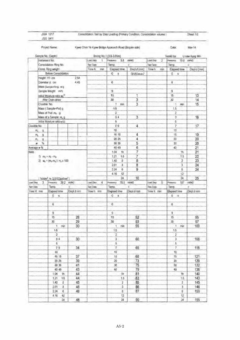
A5-2

A5-3

A5-4

A5-5

A5-6

A5-7

A5-8

A5-9

A5-10

A6-1

Annex 6: Consolidation Curve and yield point on an e-log P curve

(1) Figure: Relation e - Log p, 1) Plot the point on a graph paper

with Vertical axis: e , Horizontal axis: log p

2) Connect the plotted points and connect by smooth curve

3) Calculate Consolidation Ratio Cc Cc = (ea-eb)/log (pb/pa)

(2) Consolidation Yield Pressure Casagrande's Method

1) Seek a point A on an e-log p curve, at a Maximum curvature.

2) Draw a horizontal line A-B and tangential line A-C from the point A.

3) Intersection E of the above Bisector of two lines and extension of the straight line of e-log p, which represent the steepest slope of the normal consolidation area. Make horizontal value of E as a pc

Mikasa's Method

1) Seek a tangential contact point A on a e-log p curve, where straight line with slope C'c =0.1+0.25Cc

2) Draw a straight line with slope C''c = C'c/2

3) Horizontal coordinate of Intersection B between the above line and extension of the straight line

A

E

pc

Cc

log p

e or f

ea (fa)

pa log p

e or f

pb

eb (fb)

Cc

B

C

D

A

B

pc

C''c C'c

Cc

1/2

log p

e or f

A７-1

Annex 7: Plotting of log mv- log p curve

1) Plot the point on log –log graph paper (Annex 1. Cv,mv – P relation page A-7)

With vertical axis log mv Horizontal axis Average Consolidation pressure.

2) Connect the plotted points

A７-1

Annex 8: Sample of obtaining e-log p curve by MS Excel

Load (KN/m2)Depth γw Moisture Dry γd Gs ρs 9.8 19.6 39.2 78.6 157 314

BH-No.1 m lbs/cu.ft % lbs/cu.ft KN/m3 g/cm3 KN/m3 Consolidation (percent)1.5-1.95 35.5 80.0 12.57 2.55 25.01 1.3 2.2 4.2 6.8 9.8 15.33-3.65 34.4 86.9 13.65 2.56 25.11 0.3 0.9 1.8 3.5 6.1 9.74-4.95 45.4 72.3 11.36 2.56 25.11 4.1 7.2 10.6 14.2 18.0 22.76.1-6.7 29.5 88.0 13.82 2.65 25.99 1.6 3.0 4.8 7 9.7 12.9

BH-No.21.5-1.95 35.4 80.6 12.66 2.56 25.11 2.1 3.4 4.6 6.1 8.3 13.33-3.65 33.6 86.6 13.60 2.56 25.11 0.1 0.7 2.2 4.3 6.7 9.54-4.95 42.6 74.5 11.70 2.56 25.11 2.9 4.9 7.4 10 12.9 16.66.1-6.7 27.4 93.0 14.61 2.58 25.30 0.8 1.7 2.9 4.6 6.5 9.1

Calculation of e from above data e0=(ρs/ρd)-1 Void ratio: e=(e0+1) x (1-p /100)-12.25 9.8 19.6 39.2 78.6 157 314

1.5-1.95 Br-1 Br1-1 0.99 0.964 0.946 0.906 0.855 0.795 0.6853-3.65 Br1-2 0.84 0.834 0.823 0.806 0.775 0.727 0.6614-4.95 Br1-3 1.21 1.120 1.051 0.976 0.897 0.813 0.709

6.1-6.7 Br1-4 0.88 0.850 0.824 0.790 0.748 0.698 0.637

1.5-1.95 Br-2 Br2-1 0.98 0.941 0.915 0.892 0.862 0.818 0.7193-3.65 Br2-2 0.85 0.844 0.833 0.805 0.766 0.722 0.6704-4.95 Br2-3 1.15 1.083 1.040 0.986 0.931 0.868 0.7896.1-6.7 Br2-4 0.73 0.718 0.702 0.682 0.652 0.619 0.574

For All Br. No.1 and No.2 Data Obtaining graphs from above data by using Graph adding function of MS excel

0.50

0.60

0.70

0.80

0.90

1.00

1.10

1.20

1.30

1 10 100 1000

Br1-1

Br1-2

Br1-3

Br1-4

Br1-4

Br2-1

Br2-2

Br2-3

Br2-4

A9-1

Annex 9: Sample of obtaining Cv and Cv – P curve by MS Excel

Determination of Cv using a Tailors square root method

Consolidation test results, Time consolidation resultsSecond Minutes Hour

BH1-2 0 15 30 1 4 9 16 25 36 49 1:04 1:21 1:40 2:01 2:24 24：00Minutes 0.25 0.5 1 4 9 16 25 36 49 64 81 100 121 144 1440

Kn/m2 SQRT(m) 0.50 0.71 1.00 2.00 3.00 4.00 5.00 6.00 7.00 8.00 9.00 10.00 11.00 12.00 18 37.959.8 1 3 3 3 4 4 4 5 6 7 7 8 8 9 9.2 10

19.6 13 14 15 16 17 19 20 20 21 21 22 23 24 24 24.7 2539.2 28 29 30 33 34 37 39 41 43 44 44 45 46 48 49.2 4878.5 52 53 55 60 65 68 73 75 79 81 83 85 86 87 88.6 90157 95 87 100 106 118 121 129 132 138 140 143 145 146 150 151.4 155314 165 170 173 180 190 200 214 218 220 225 230 233 236 240 241.2 247

BH1-3 0 15 30 1 4 9 16 25 36 49 1:04 1:21 1:40 2:01 2:24 24：00Minutes 0.25 0.5 1 4 9 16 25 36 49 64 81 100 121 144 1440

Kn/m2 SQRT(m) 0.50 0.71 1.00 2.00 3.00 4.00 5.00 6.00 7.00 8.00 9.00 10.00 11.00 12.00 18 37.959.8 10 20 40 60 80 86 88 95 98 100 100 101 102 102 102.2 103

19.6 143 150 153 159 165 169 171 172 174 176 177 178 180 180 181.2 18339.2 195 212 214 217 232 235 238 240 243 246 253 259 263 265 265.5 27078.5 280 290 303 320 330 340 345 348 348 349 350 351 354 356 356.7 363157 378 385 400 430 433 437 440 443 447 448 449 450 451 452 452.9 458314 475 485 510 530 548 550 552 553 555 558 560 563 568 572 572.7 577

BH1-4 0 15 30 1 4 9 16 25 36 49 1:04 1:21 1:40 2:01 2:24 24：00Minutes 0.25 0.5 1 4 9 16 25 36 49 64 81 100 121 144 1440

Kn/m2 SQRT(m) 0.50 0.71 1.00 2.00 3.00 4.00 5.00 6.00 7.00 8.00 9.00 10.00 11.00 12.00 18 37.959.8 15 18 25 30 33 36 36 38 38 38 39 39 40 40 40.0 41

19.6 43 46 50 60 62 63 64 65 65 65 67 68 71 72 72.0 7739.2 95 100 102 107 108 110 112 118 119 120 120 120 121 121 121.0 12378.5 146 150 160 165 167 168 170 171 172 172 173 175 176 177 177.0 180157 200 210 220 228 230 233 235 236 238 238 238 240 242 243 243.0 247314 266 289 300 309 312 314 315 317 318 319 320 324 325 326 326.0 329

Obtaining graphs from above each data by using Graph adding function of MS excel

BH1-2 BH1-3 BH1-4

Vview of the upper 3 curves portion by enlarged vertical axis dimension of the above graph for easy to read t90.

0

50

100

150

200

250

300

0.00 5.00 10.00 15.00 20.00

9.8

0

100

200

300

400

500

600

700

0.00 5.00 10.00 15.00 20.00

9.8

0

50

100

150

200

250

300

350

400

0.00 5.00 10.00 15.00 20.00

0

10

20

30

40

50

60

0.00 5.00 10.00 15.00 20.00

9.8

This column inserted for easy to handle following figure

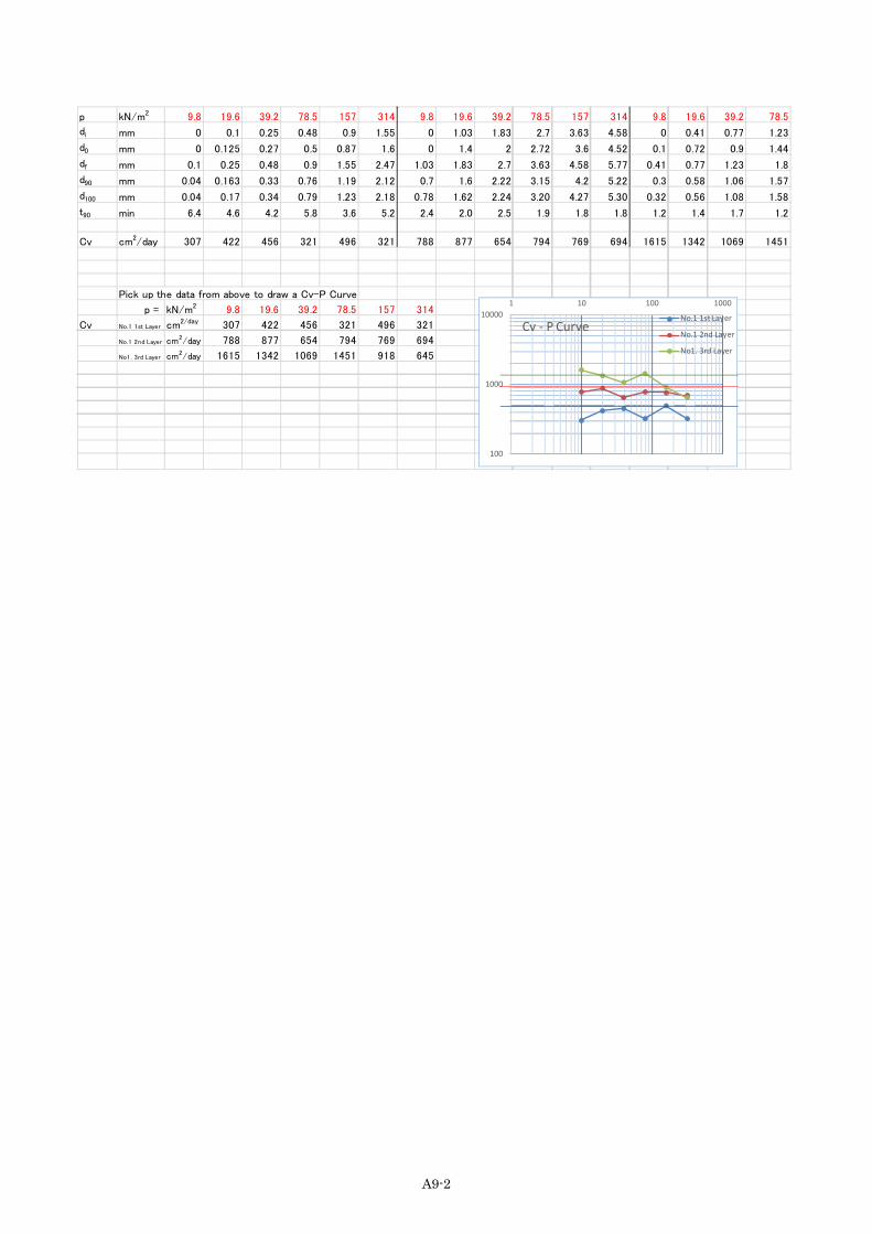
A9-2

p kN/m2 9.8 19.6 39.2 78.5 157 314 9.8 19.6 39.2 78.5 157 314 9.8 19.6 39.2 78.5

di mm 0 0.1 0.25 0.48 0.9 1.55 0 1.03 1.83 2.7 3.63 4.58 0 0.41 0.77 1.23

d0 mm 0 0.125 0.27 0.5 0.87 1.6 0 1.4 2 2.72 3.6 4.52 0.1 0.72 0.9 1.44

df mm 0.1 0.25 0.48 0.9 1.55 2.47 1.03 1.83 2.7 3.63 4.58 5.77 0.41 0.77 1.23 1.8

d90 mm 0.04 0.163 0.33 0.76 1.19 2.12 0.7 1.6 2.22 3.15 4.2 5.22 0.3 0.58 1.06 1.57

d100 mm 0.04 0.17 0.34 0.79 1.23 2.18 0.78 1.62 2.24 3.20 4.27 5.30 0.32 0.56 1.08 1.58

t90 min 6.4 4.6 4.2 5.8 3.6 5.2 2.4 2.0 2.5 1.9 1.8 1.8 1.2 1.4 1.7 1.2

Cv cm2/day 307 422 456 321 496 321 788 877 654 794 769 694 1615 1342 1069 1451

Pick up the data from above to draw a Cv-P Curve

p = kN/m2 9.8 19.6 39.2 78.5 157 314

Cv No.1 1st Layer cm2/day 307 422 456 321 496 321

No.1 2nd Layer cm2/day 788 877 654 794 769 694

No1. 3rd Layer cm2/day 1615 1342 1069 1451 918 645

100

1000

100001 10 100 1000

Cv - P CurveNo.1 1st Layer

No.1 2nd Layer

No1. 3rd Layer

1000

A10-1

Annex 10: JIS Data Format Sheets

Consolidation test by Step loading (Primary Condition, Consolidation

volume)

Consolidation test by Step loading (Consolidation volume)

Consolidation test by Step loading (d-√t curve)

Consolidation test by Step loading (consolidation-time curve)

Consolidation test by Step loading (calculation table)

Soil consolidation Test by Stage Loading, Constant strain speed (Cv, mv-P

relation)

Soil consolidation Test by Stage Loading, Constant strain speed

Annex 1. Schedule of Approach embankment Plan

Annex 2. Sample of Table contents for Observation analysis result report

A10-2

JIS A 1217 Consolidation Test by Step Loading (Primary Condition, Consolidation volume )JGS 0411

Project Name: Date:

Sample No. (Depth) Tested by:Instlement No. Load.Step Load.StepConsolidation Ring No. Test Date Temp. ℃ Test Date Temp. ℃

Conol. Ring weight T ime Elapsed time Displ.d mm Time Elapsed time Displ.d mm0 0

Height H1: cm s sDiameter d : cmMass (Sample+Ring): m t gSample Weight m 0

1)

Initial Moisture ratio:w 01)

Crusible No. 1 min 1 minMass ( Sample+Pot) g 1.5 1.5Mass of Pod :m0 : g 2 2Mass of a Sample: m s g 3 3Initial Moisture ratio (by sample turning) 5 5

Crusible No. 7 7m a g 10 10m b g 15 15m c g 20 20w % 30 30

Average w % 40 40Note : 1h 1h

1) m0 = mt - mR 1.5 1.52) w0 = (m0-ms) / ms x 100 2 2

3 36 6

12 12[ 1kN/m2 ≒ 0.0102kgf/cm2 ] 24 24

Load.Step Pressure:p kN/M2 Load.Step Load.StepTest Date Temp. ℃ Test Date Temp. ℃ Test Date Temp. ℃

Time Elapsed time Displ.d mm Time Elapsed time Displ.d mm Time Elapsed time Displ.d mm0 0 0s s s

1 min 1 min 1 min1.5 1.5 1.5

2 2 23 3 35 5 57 7 7

10 10 1015 15 1520 20 2030 30 3040 40 40

1h 1h 1h1.5 1.5 1.52 2 23 3 36 6 6

12 12 1224 24 24

Pressure:p kN/M2 Pressure:p kN/M2


After Oven-dried

Before Consolidation

A10-3

JIS A 1217 Consolidation Test by Step Loading (Consolidation volume )JGS 0411

Project Name: Date:

Sample No. (Depth) Tested by:Load.Step Pressure:p kN/M2 Load.Step Load.StepTest Date Temp. ℃ Test Date Temp. ℃ Test Date Temp. ℃


1 min 1 min 1 min1.5 1.5 1.5

2 2 23 3 35 5 57 7 7

10 10 1015 15 1520 20 2030 30 3040 40 40

1h 1h 1h1.5 1.5 1.52 2 23 3 36 6 6

12 12 1224 24 24

Load.Step Pressure:p kN/M2 Load.Step Load.StepTest Date Temp. ℃ Test Date Temp. ℃ Test Date Temp. ℃


1 min 1 min 1 min1.5 1.5 1.5

2 2 23 3 35 5 57 7 7

10 10 1015 15 1520 20 2030 30 3040 40 40

1h 1h 1h1.5 1.5 1.52 2 23 3 36 6 6

12 12 1224 24 24



A10-4

A10-5

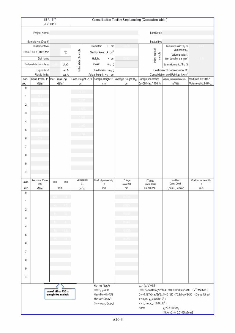
A10-6

JIS-A 1217JGS 0411

Test Date :

Tested by :4.450 Moisture ratio: w0 % 34.4

℃ 15.553Void ratio: e0,

Volume ratio: f02.540 Wet density: ρｔ　g/㎝3 18.18

2.56 g/㎝3 Saturation ratio: Sr0 %

wl % 534.37 wp % 1.342

Load. Cons. Press. P Sample Height: H Average Height: Hav. Completion strain: Volume compressibility : mv Void ratio e=H/Ha-1step kN/m2 cm cm Δε=ΔH/Hav. * 100 % m2/ kN Volume ratio: f=H/Hav.

0 0 2.54 0.8932.535 0.394 4.025E-04

1 9.8 2.53 0.8852.523 0.595 6.068E-04

2 19.6 2.515 0.8742.504 0.919 4.687E-04

3 39.2 2.492 0.8572.471 1.700 4.325E-04

4 78.5 2.45 0.8252.419 2.563 3.265E-04

5 157 2.388 0.7792.341 4.015 2.558E-04

6 314 2.294 0.709

7

8

9

10

Load. Ave. cons. Press.:pav t90 t50

Coeff. of permeability:k

1st stageCons.:ΔHi

1st stage Cons. Ratio

ModifiedCons. Coeff.

Coeff. of permeability:k'

step kN/m2 m/s cm r = ΔHi /ΔH Cv' = r Cv cm2/d m/s0

4.9 6.6 14 297.0 32.5 1.232E-11 0.075 7.500 2227.3 8.7861

14.7 4 4.2 485.2 107.4 3.033E-11 0.023 1.533 743.9 4.4242

29.4 11 10 173.8 44.4 8.393E-12 0.015 0.652 113.3 0.5213

58.85 13 8 143.3 54.1 6.384E-12 0.044 1.048 150.1 0.6364

117.75 19 6.8 93.9 61.0 3.160E-12 0.105 1.694 159.1 0.5095

235.5 35 11 47.8 35.3 1.258E-12 0.085 0.904 43.2 0.1086

7

8

9

10

Here: γｗ=9.81 kN/m3

[ 1kN/m2 ≒ 0.0102kgf/cm2 ]

Hav=(Hn+Hn-1)/2 Cv =0.197x(Hav/2)^2x1440 / t50 =70.9xHav̂ 2/t50　（Curve fitting）

Mv=(Δε/100)/ΔP k = cv mv γｗ / (8.64x108 )Srs = w0 ρs/ (es ρw) k' = cv

' mv γｗ / (8.64x108 )

Cons coeff.:Cv

min cm2/d

Hs= ms / (ρsA) pav= (p:*p')^0.5Hn=Hn-1- ΔHn Cv=0.848x(Hav/2)^2*1440 /t90 =305xHav̂ 2/t90　（√t Method）

157 0.094

39.3 0.042

78.5 0.062

19.6 0.023

9.8 0.01

9.8 0.015

Incr. Press.: Δp Cons. Height: ΔHkN/m2 cm

Liquid limit: Dried Mass: md g Coefficient of Consolidation: CcPlastic limits: Actual height: Hs cm Consolidation yield Point: pc kN/m2

Instlement No.

Initia

l stat

e of s

ample

Diameter: D cm

Initia

l stat

e of

samp

leRoom Temp. Max~Min Section Area: A cm2

Soil name Height: H cm

Soil particle density: ρs mass: ms g

Consolidation Test by Step Loading (Calculation table )

Project Name:

Sample No. (Depth)

one of t90 or T50 is enough foe analysis one of t90 or T50 is enough foe analysis one of t90 or T50 is enough foe analysis

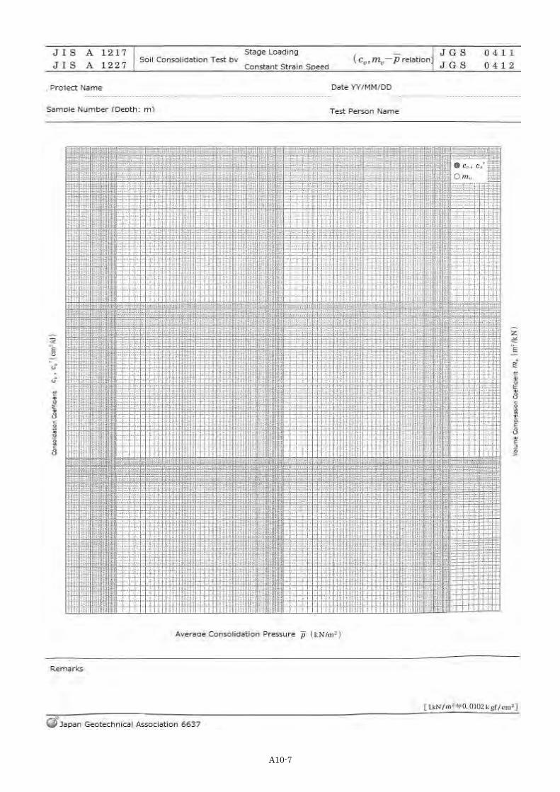
A10-7

A10-8

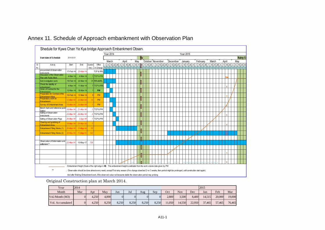
A11-1

Annex 11. Schedule of Approach embankment with Observation Plan

Original Construction plan at March 2014.

Year 2014 Year 2015Start date of Schedule 2014-03-01 Ra Rainy Se

ID Activ ity Start End Duration Office 1 8 15 22 29 5 12 19 26 3 10 17 24 11 18 25 1 8 15 22 29 6 13 20 27 3 10 17 24 31 7 14 21 28 7 14 21 28 4 11 18 25 2 9 16 23 30No. (day ) in Charge Sat Sat Sat Sat Sat Sat Sat Sat Sat Sat Sat Sat Sat Sat Sat Sat Sat Sat Sat Sat Sat Sat Sat Sat Sat Sat Sat Sat Sat Sat Sat Sat Sat Sat Sat Sat Sat Sat Sat Sat Sat Sat Sat Sat Sat Sat Sat

procurement of observationInstruments 17-Feb-14 23-Mar-14 TCP & RRL O O O ODiscussion of the ObservationPlan with Public Work 4-Mar-14 4-Mar-14 1 TCP & PW 9mSoil investigation work 19-Feb-14 22-Mar-14 31 RRL&SRL O O O OCheck the stability ofembankment 4-Mar-14 11-Mar-14 7 TCP & RRL O 8Order of Contract for theEmbankment 12-Mar-14 18-Mar-14 1 PW OPreparation for Contract of theEmbankment Work 10-Feb-14 12-Mar-14 5 PW O O 7Preparatory work forEmbankment 12-Mar-14 22-Mar-14 10 PW O OSurvey of Embankment Area 18-Mar-14 25-Mar-14 7 PW O 6Bench mark and reference pointSetting 18-Mar-14 21-Mar-14 3 TCP & PWSetting of ObservationInstruments 23-Mar-14 26-Mar-14 3 TCP & PW 5Setting of Observation Pegs 26-Mar-14 2-Apr-14 7 TCP & PW OClearing and grabbing ofEmbankment Area 18-Mar-14 25-Mar-14 7 O 4Embankment Filling Works (1) 26-Mar-14 15-May-14 50 O O O O O O OEmbankment Filling Works (2) 30-Nov-14 11-May-15 162 O O O O O O O O O O O O O O O O O O O 3 O O O

Observation of Deformation andsettlement ** 25-Mar-14 10-May-17 730 O O O O O O O O O O O O O O O O O O O O O O O O O O O O O O O O O O O O 2 O O O O O O

1

0.3 0.6 0.9 0.9 1.2 1.5 2.1 2.4 3.0 3.3 3.8 3.9 4.2 4.5 4.8 5.1 5.4 5.7 6.3 7.8 8.1 9 0: Embankment Height (Scale of the right edge in M) This embankment height is estimated from the work volume data given by PW

** : Observation should be done almost every week, except First rainy season (if no change obserbed 2~or 3 weeks, then period might be prolonged, until construction start again)

And after finishing Embankment work, if the observed value not becaome stable the observation period may prolong

Shedule for Kywe Chan Ye Kya bridge Approach Embankment Observ

AprilOctober MayMarch April May November JanuaryDecember MarchFebruary

Year 2014 2015Month Mar Apr May Jun Jul Aug Sep Oct Nov Dec Jan Feb Mar

Vol./Month (M3) 0 4,250 4,000 0 0 0 0 2,800 3,500 8,400 14,515 20,000 19,000

Vol. Accumulated 0 4,250 8,250 8,250 8,250 8,250 8,250 11,050 14,550 22,950 37,465 57,465 76,465

A12-1

Annex 12. Sample of Table contents for Observation analysis result report

Summary 1. Project Overview

Project Purpose, Project Location, Dimension and so on. 2. Topography & Geology of the site

Description of Topography of the site Description of Geology of the site

3. Construction Works Description of construction works

3.1 Applied Construction Method Description of actually selected construction Method and any counter measure adopted

3.2 Slop Stability study Study result of slop stability and any counter measure selected before construction start

3.3 Consolidation settlement study Study result of consolidation settlement and any counter measure adopted before construction.

3.4 Designed counter measure Designed counter measure adopted from above study and expectation of it.

4. Field observation $ measurement 4.1 Introduction

Field observation purpose and measurement items. Arrangement of measuring Instruments Plan of measurement interval

4.2 Settlement measurement Settlement board and pore pressure gauge arrangement Setting of supervise criteria

4.3 Slope stability related measurement Arrangement of surface movement measuring pegs and setting of inclinometer guide pipes. Measuring method by Total station survey. Setting of supervise criteria

5. Construction Results 5.1 Measurement results of Settlement

Relation Curve of Filling height – Settlement Comparison of Prediction and Observed

5.2 Residual settlement Prediction of residual settlement from observation result. Any counter measure or study results

5.3 Influence to adjacent ground Relation of filling height and Actual surface or ground movement Influence on surrounding structure or ground and actual countermeasure taken.

6. Proposal for future construction work. Finding obtained from the observation Recommendation for future work

A-13-1

Annex13 (sample) Specification of Embankment at Approach Road to Bridges

Contents

1. Preparation work 1.1 Top survey P1

2. Clearing & Grubbing P2

3. Borrow Excavation P2

4. Embankment P2

5. General Requirement 5.1 Language P8

5.2 Meeting

5.3 Engineers Facilities and Service

5.4 Submittals

Red one shows the items to be decided by PW. 1.1. Topographic Survey Works

Site Items Approach section Remarks Setting of Bench Marks Both approach One on Abutment and Two Reference point at

ground 150m from the edge of embankment Plan Survey Width 70m Drawing Scale 1/500 (Size of drawing is A-3)

Centerline Survey 20m Interval Drawing Scale 1/500 (Size of drawing is A-3)

Profile Leveling 20m interval Drawing Scale 1/500 (Size of drawing is A-3) Cross Sectional Survey Width 70m / section 20m interval Drawing Scale 1/500 (Size of drawing is A-3)

Cross Sectional Survey of Borrow area 20m interval Drawing Scale 1/500 (Size of drawing is A-3)

a) Drawings

One set of original drawings (and the as-built drawings) with soft copies. b) Total Station Digital data

It shall include survey record, survey calculation and accuracy control record.

2. Clearing and Grubbing In areas under roadway embankments, from which top soil or unsuitable materials are to be removed

or which are designated to be compacted, all grass, stumps and roots shall be removed to a depth at

least 30 cm below the original ground surface and at least 30 cm below the bottom of the designed

lowest embankment layer.

“Cleared material” shall be disposed to the place approved by the Engineer in advance.

Otherwise, “Cleared material” stocked could be used for the surface of the slope of the embankment.

The work as provided above shall neither be measured nor paid directly or separately

A-13-2

3. Borrow material This Section describes requirements and procedures for the clearing of “borrow area” and the

excavation and hauling of material. “Borrow areas” include the area legally obtained by the Contractor

and approved by the Engineer.

(a) Before any borrow is excavated, the Contractor shall clear the ground surface of the “borrow

area” and notify the Engineer to jointly make “Area survey of the topography” and provide necessary

cross-sections.

(b) Excavation within 30m areas from the edge of the embankment will not be allowed.

(c) Performance of this work shall not be paid for separately, but shall be considered as a

subsidiary obligation of the Contractor for which full payment is in accordance with applicable unit

prices of embankment. 4. Embankment Construction This Section describes requirements and procedures for the construction of the roadway embankment

and sub-grade, including the requirements for setting out the work, staking and surveying.

a) Contractor shall submit complete sets of Detailed Plan, Shop-Drawings and Schedules for

embankment construction to the Engineer for review and approval.

b) The plan for embankment construction by re-using the remaining material from Embankment for

Settlement (and counterweight used for soft-soil improvement and slope stabilization, if ordered by the

Engineer) shall include an approximate time schedule, the location (Station or road section) of the

material to be re-used, the location where it is intended to be placed, detailed schedule of quantities,

etc.,

c) The approved plan shall be used for monitoring of quantities and shall be updated continuously

on a monthly basis by the Contractor in coordination with the Engineer. 4.1. Materials The material for embankment, borrow material, sand or granular material, or classified soil, might be

provided from Borrow within or in the surroundings of the Project area or from a source approved by the

Engineer, or obtained from excavation at site.

Top 50 cm Layer (SUB-GRADE)

The material used for embankment construction in the top 50 cm layer (sub-grade) is the soil with the

minimum CBR value of 5% (saturated sampling for 96 hour) or equivalent. The Contractor shall mix

sand or aggregate, if necessary, and compact to get the specified CBR.

Layers more than 50 cm below Sub-grade

Layer of 50 cm below Sub-grade (Embankment) shall be Borrow material. (Sand layer mixing might

be ordered, if necessary. But not fixed)

Cleared Material for Slope

Materials to be used on the slope surface shall receive the prior approval by the Engineer, 4.2. Setting out the Work, Staking and Surveying Notice for Starting the Work:

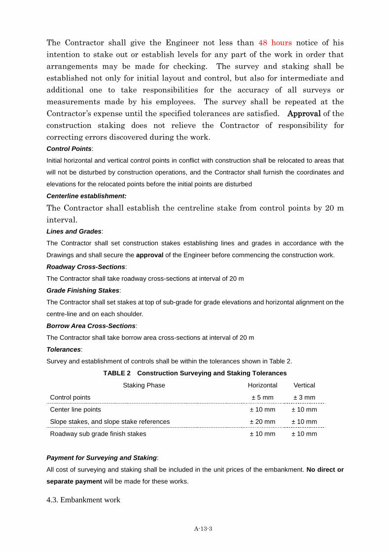
A-13-3

The Contractor shall give the Engineer not less than 48 hours notice of his intention to stake out or establish levels for any part of the work in order that arrangements may be made for checking. The survey and staking shall be established not only for initial layout and control, but also for intermediate and additional one to take responsibilities for the accuracy of all surveys or measurements made by his employees. The survey shall be repeated at the Contractor’s expense until the specified tolerances are satisfied. Approval of the construction staking does not relieve the Contractor of responsibility for correcting errors discovered during the work. Control Points:

Initial horizontal and vertical control points in conflict with construction shall be relocated to areas that

will not be disturbed by construction operations, and the Contractor shall furnish the coordinates and

elevations for the relocated points before the initial points are disturbed

Centerline establishment:

The Contractor shall establish the centreline stake from control points by 20 m interval. Lines and Grades:

The Contractor shall set construction stakes establishing lines and grades in accordance with the

Drawings and shall secure the approval of the Engineer before commencing the construction work.

Roadway Cross-Sections:

The Contractor shall take roadway cross-sections at interval of 20 m

Grade Finishing Stakes:

The Contractor shall set stakes at top of sub-grade for grade elevations and horizontal alignment on the

centre-line and on each shoulder.

Borrow Area Cross-Sections:

The Contractor shall take borrow area cross-sections at interval of 20 m

Tolerances:

Survey and establishment of controls shall be within the tolerances shown in Table 2.

TABLE 2 Construction Surveying and Staking Tolerances

Staking Phase Horizontal Vertical

Control points ± 5 mm ± 3 mm

Center line points ± 10 mm ± 10 mm

Slope stakes, and slope stake references ± 20 mm ± 10 mm

Roadway sub grade finish stakes ± 10 mm ± 10 mm

Payment for Surveying and Staking:

All cost of surveying and staking shall be included in the unit prices of the embankment. No direct or

separate payment will be made for these works. 4.3. Embankment work

A-13-4

(a) Roadway embankment materials shall be placed in horizontal layers not exceeding the

thicknesses of 30cm, in loose measurement, and shall be compacted as specified, tested for density

and accepted by the Engineer, before the next layer is placed.

(b) Embankment layers shall be compacted and shaped to a 4% grade from the center to both sides

for drainage of rainwater.

(c) Effective spreading equipment shall be used on each lift to obtain uniform thickness prior to

compacting. As the compaction of each lift progresses, continuous leveling and manipulating will be

required to assure uniform density.

(d) Where placing and/or compaction of material under saturated or flooded conditions cannot be

avoided, the Contractor shall submit to the Engineer for approval his proposed methods to ensure

adequate compaction.

(e) Dumping and rolling areas shall be kept separate, and another shall cover no lift until compaction

complies with the requirements of this Specification Section. 4.4. Compaction of Embankment Material (a) Embankment layers shall be placed and compacted to a uniform density at moisture content within

the range of 5% less than optimum moisture content to 3% more than optimum moisture content.

Acceptance of compaction degree is shown in bellow Table 3.

(b) Water shall be added or removed, if necessary, in order to obtain the required density.

(c) Removal of excessive water shall be accomplished through aeration by plowing, balding, disking,

or other methods satisfactory to the Engineer.

(d) Sub-grade Layer: Proof rolling shall be conducted after finishing by more than 25 tons weight

roller on the place directed by the Engineer. If the deflection is more than 5mm, the place shall be

checked and replaced, if necessary, by the instruction of the Engineer.

(e) Compaction of Slope: The Contractor shall compact the slope by appropriate methods to prevent

the water erosion. All earth slopes shall be reasonably uniform, without any noticeable break, and in

reasonably close conformity with the Drawings, or as directed by the Engineer. The Contractor shall

remedy the work, if the erosion occurred within three month after the completion of the work.

(f) Compaction in the existing water canal: The Contactor shall excavate the bottom of canal up to

minimum 50cm, and place the appropriate material as the first layer to get the base for the compaction

of upper layer as approved by the Engineer.

(g) Compaction of backside materials of abutment: The backside of abutment shall be filled with

granular material as approved by the Engineer. Maximum thickness of one layer shall be 30cm and

compaction degree shall be as shown in Table 3.

Table 3 Requirements for Compaction

Compaction degree *

Top 50 cm Layer (Sub-grade) 98% (AASHTO T180)

Layers more than 50 cm below Sub-grade 95% (AASHTO T180)

Cleared material on Slope 95% (AASHTO T180)

Back side materials of abutment 95% (AASHTO T180)

A-13-5

(h) Testing Method: The Contractor shall, during progress of the Works, carry out density tests of

compacted material in accordance with AASHTO T191, T205, or other approved field density tests,

including the use of properly calibrated nuclear testing devices. And, if the result of any test shows that

the density is less than the required density, the Contractor shall rectify the work. The test shall be

made to the full depth of the layer at locations directed by the Engineer.

(i) Testing Frequency: At least one group of three in-situ density tests shall be carried out for every

1,500 m2 of each layer of compacted fill. 4.5. Compaction Equipment Compaction equipment shall satisfy compaction requirements of these specifications without

detrimentally affecting the compacted material. The equipment shall be a modern, standard, efficient

compacting units approved by the Engineer. The compacting units may be of any type, provided that

they are capable to compact each lift of material as specified and meet the minimum requirements as

contained herein. 4.6. Compaction Trial Before commencing the formation of embankments, the Contractor shall conduct trial compaction for

Borrow material under the supervising of the Engineer about the relation between the types of

compaction equipment, and the number of passes required and the method of adjusting moisture

content. 4.7. Method of Measurement a) The quantities for Embankment Construction shall be measured in cubic meters and computed (by

cross sections surveying immediately before/after work completion of a part or whole) in compacted

volume approved by the Engineer.

b) The volume of embankment shall be computed from the cross-section areas bounded by the

upper lines calculated from the Shop Drawings and the above mentioned survey, the designed slope

lines, and bottom planes of the sub-grade or a plane defined by the Engineer.

c) The embankment constructed as per counter-weight and for settlement, if required, shall be

measured and paid for at the same price approved for the road embankment.

d) Settlement volume compensation shall be calculated according to the height of embankment by

using the average settlement depth (per meter for embankment height) of “settlement boards” installed

prior to the commencement of the embankment work. If the Contractor gave the damage to the

installed settlement board during the embankment work, no compensation will be done for the

settlement.

e) The quantities for Slope Construction by “Cleared material” shall be measured in cubic meters and

computed in compacted volume and in accordance with the Drawings.

f) Contractor shall submit the summary Table of the filled materials, which includes the Table of

excavated volume at borrow area by the computation from cross section survey of “borrow area”. 4.8 Basis of Payment

A-13-6

a) The accepted quantities, measured as provided above, shall be paid at the contract price per unit

of measurement for the pay items of the Bill of Quantities listed below.

b) Sand, (used as sandwich layer among borrow layer, or used in another places, if required by the

Engineer,) shall be measured by the hauled volume by Track to the site. The Contractor shall receive

the checking on site by preparing the list of tracks with each hauling volume This hauled volume shall

be deducted from the volume of borrow materials computed by the above cross sectional survey.

c) Payment shall be full compensation for the entire work prescribed in this Section including

preparation of foundations for embankment, layering, blending (if required), watering, material and

construction of cohesive slope, temporary drainage, hauling, compacting, shaping, trimming, finishing

and maintaining embankments and for furnishing all labor, materials, tools, equipment and any

incidentals to complete the work as shown on the Drawings and as required in accordance with these

Specifications and/or as directed by the Engineer.

Pay Item Description Unit

Construction of Subgrade (50 cm Layer) M3

Construction of Embankment (below Subgrade) M3

Construction by Sand layer M3

Construction of backside of abutment M3 5. General Requirement There is no separate payment for this clause. It shall be included in the Item of Embankment. 5.1. Language All maps, drawings, draft and final reports and letters shall be in English.

5.2. Meeting The Contractor shall provide sufficient support to the Engineer for preparing and holding periodic

meetings for coordination and reporting with all the Project’s stakeholders concerned.

5.3. Engineers Facilities and Services The Contractor shall provide facilities on site for supervisory Engineers in accordance with the time

periods.

The Contractor shall cooperate on the installation of observation instrument which will be installed by

the Engineer.

5.4. Submittals a) The Contractor shall prepare and submit to the Engineer a list of delivery forecasts for each

significant material/equipment required for the Project. The listing shall show the target order dates,

shipping and receiving dates and quantities of each required material/equipment.

Implementation schedule The Contractor shall submit to the Engineer, for his review and approval, a detailed Mobilization

Program including mobilization and de-mobilization time schedule

It shall describe about total work volume calculation with daily output volume.

b) Progress Report

A-13-7

Every end of two weeks, progress report shall be submitted by one sheet of A4 size.

d) Contractor shall submit all of the test results record of Quality Control to the engineer.

5.5. Project Safety (not described)

5.6. Environmental Control and Protection (not described)

5.7. Laboratory and Engineer’s Equipment (not described)

5.8. Quality Control (not described)

A-13-1

Annex 14: Answer of Drills

Answer of Drill Drill 1: Connect by line, which has direct relations (Time limit: 15 minutes)

- Internal friction angle Ground settlement - - Inclinometer

- Consolidation test Slope stability - - Settlement Board

6 - Pore pressure gauge Drill 2:

- Visual inspection Original Ground strength - - CBR

New Embankment strength - - N-value Pavement strength - - Cone Penetration value

7 - K-value Drill 3:

- Soil stratum thickness - N-value

Boring log - - Depth of sampling - Soil color

Lab test of boring sample - - Specific gravity - LL, PL, PI

Soil Classification - - Permeability - Moisture Contents - Grain size distribution 12 - Wet density

Drill 4: Internal friction angle φ is minimum 45 degree? not correct

Drill 5: Shear strength will be produced by the friction strength of soil particles, and shear strength is

zero, if there is no overburden pressure? not correct

S=C+σtanφ Drill 6: Shear strength of Clay is produced by cohesion only? not correct

Drill 7: Shear strength of Sand is produced by internal friction angle? correct

Drill 8: Real shear strength is produced by internal friction angle not only for Sand but also for Clay?

correct

Drill 9: If there is adhesion, cohesion will be added to shear strength? correct

Drill 10: Visual shear strength is presented by internal friction angle in case of Sand and by cohesion in

case of Clay? correct S=σtanφ

--

-

-

-

--

-

-

Inclinometer-

A-13-2

Drill 11.

Drill 12. H= 800 cm

e0= 1.65

e= 1.41

e0-e= 0.24

1+e0= 2.65

S= 72 cm

Drill.13

1st layer 2nd layer

Gs= 2.15 1.68 tf/m3

Gub= 1.15 0.68

tf/m3

H(m)= 4 6

m

σ'= 4.6 2.04 Po=Σσ'= 6.64 tf/m2

Effective stress in the middle of clay layer after embankment Gs= 2

H= 3

ΔP= 6 P1= Po+ΔP= 12.64 tf/m2

Consolidation settlement volume

Cc= 0.375

e0= 1.811 1+eo= 2.81

log(Po+ΔP)/Po = log 1.90 = 0.28

S= Cc/(1+e)*log(Po+ΔP)/Po= 0.22 (m)

Gs= 2.72

Gs*γ

w= 2.72

e= 0.77 1+e= 1.77 γd= 1.54 t/m3

higher than Sr= 93 Sr*e= 71.6 w= 0.26

water γt= 1.94 t/m3

saturated Sr= 100 Sr*e= 77 w= 0.28

γsat= 1.97 t/m3

γsub= 0.97 t/m3

higher water h= 3

σ'= 5.82 t/m2

under water

3

σ'= 2.92 t/m2

σz'= 8.74 t/m2

A-13-3

Drill 14

1st layer 2nd layer 3rd laer Fill

H= 3 1 4 5

γt= 17 17 18 20

γ'= 17 7 8 20

Weight= 51 7 32 100

Po= 26 4 16 50

ΣPo=

55 74

ΣP1= 126 155 174

H (m) γt γ' P0 ΣPo ΣP1

5 20 100

3 17 26 26 126

1 17 7 4 55 155

4 18 8 16 74 174

Drill 15.

H

(m) z (m) a/z b/z I ΣP1

ΔP=I*

ΣP1*2 ΣPo

e0 from

Figure

e1 from

Figure S

Total

S

5

3 1.5 6.7 3.3 0.49 126 123 26

1 3.5 2.9 1.4 0.48 155 148 55 0.88 0.81 0.04

4 6 1.7 0.8 0.46 174 160 74 0.88 0.81 0.15 0.19

Continue to next page

A-13-4

A-13-5

Drill 16.

1st layer 2nd layer 3rd layer

H(m) 4 6 4

Cv(cm2/day) 244 81.4 407

Hequ to 2nd layer 2.3 6.0 1.8

Total (m) 10.1

Drill 17.

Have= 1.85 cm

H= 0.925 cm

t90= 1.5 min

Tv(90%)= 0.848 (none)

Cv= 0.484 cm2/min

= 697 cm2/day

Drill 18.

Drill 19.

H= 1000 cm

Cv= 50 cm2/day

Tv(50%)= 0.197 (none)

Tv(90%)= 0.848 (none)

both darin one side unit

t50%= 985 3940 day

t90%= 4240 16960 day

Have= 2 cm

H= 1 cm

Tv(50%)= 0.197 (none)

t50%= 18 min

Cv= 0.011 cm2/min

= 15.8 cm2/day

H= 500 cm

Tv(90%)= 0.848 (none)

t(90%)= 3363 day

= 112 Month

A-13-6

Documents

The Project for Improvement of Road Technology in Disaster ...open_jicareport.jica.go.jp/pdf/12237533.pdf · 6.7.5 Peg for deformation survey ... as a sample case for practical calculation;