Embed Size (px)
Citation preview
The Time Rate of Change of Density
Let’s consider a more general cube with sides oflength ∆x, ∆y and ∆z and volume ∆V = ∆x∆y∆z
Let M(t) denote mass inside the cube at time t.Since the flux through the surface S of the cube isthe rate at which the mass is passing out of the sur-face then
ΦS = −dM
dt

Let ρ = ρ(x, y, z, t) be the density (in kilograms permeter3) at location (x, y, z) at time t seconds. If Vdenotes the interior of the solid then
M(t) =
∫ ∫ ∫V
ρ dV
If vol(S) ≈ 0 and (x, y, z) is the center of the cubethen the mass is approximated by:
M(t) =
∫ ∫ ∫V
ρ dV ≈ ρ vol(V )
M(t) ≈ ρ vol(V )
Therefore, the flux is approximated by:
ΦS = −dM
dt≈ −∂ρ
∂tvol(V )
ΦS
vol(V )≈ −∂ρ
∂t
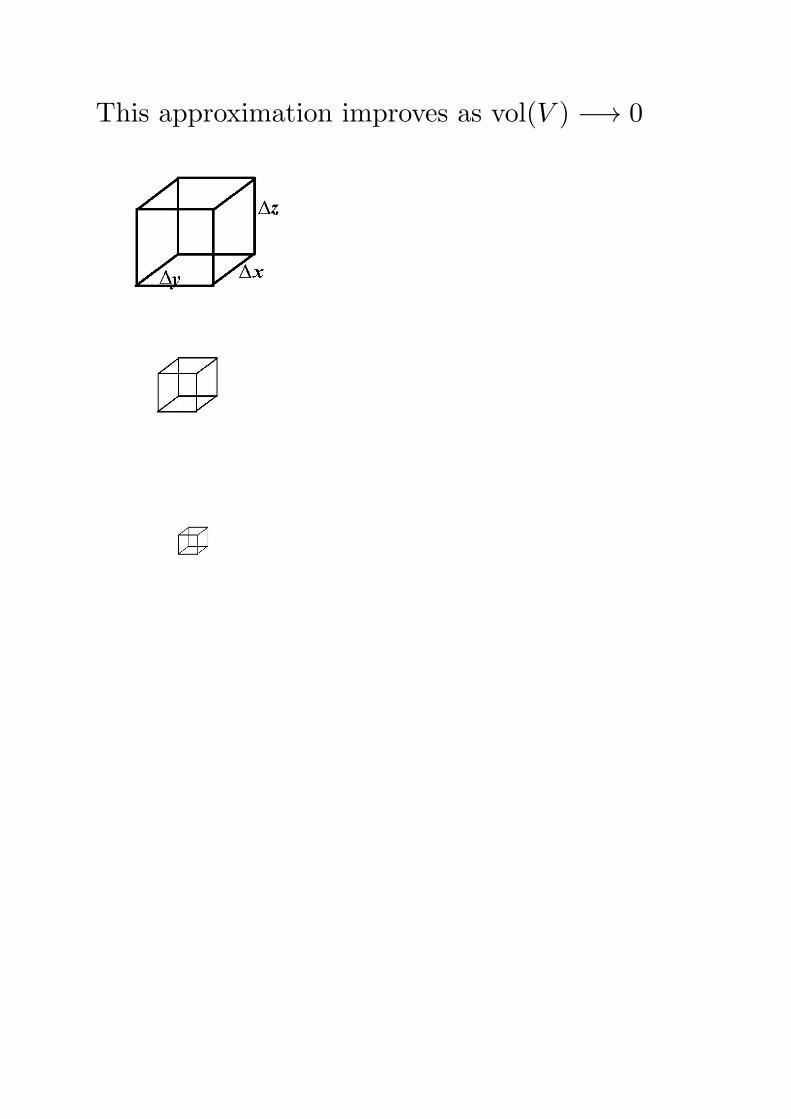
This approximation improves as vol(V ) −→ 0
In the limit,
limvol(V )→0
ΦS
vol(V )= −∂ρ
∂t
This is the divergence of the vector field F⃗.
div F⃗ = −∂ρ
∂t
Partial Derivative Formula for div F⃗
Recall that the derivative of f(x) is given by:
f ′(x) = limh→0
f(x+ h)− f(x)
h
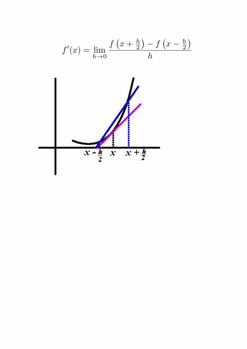
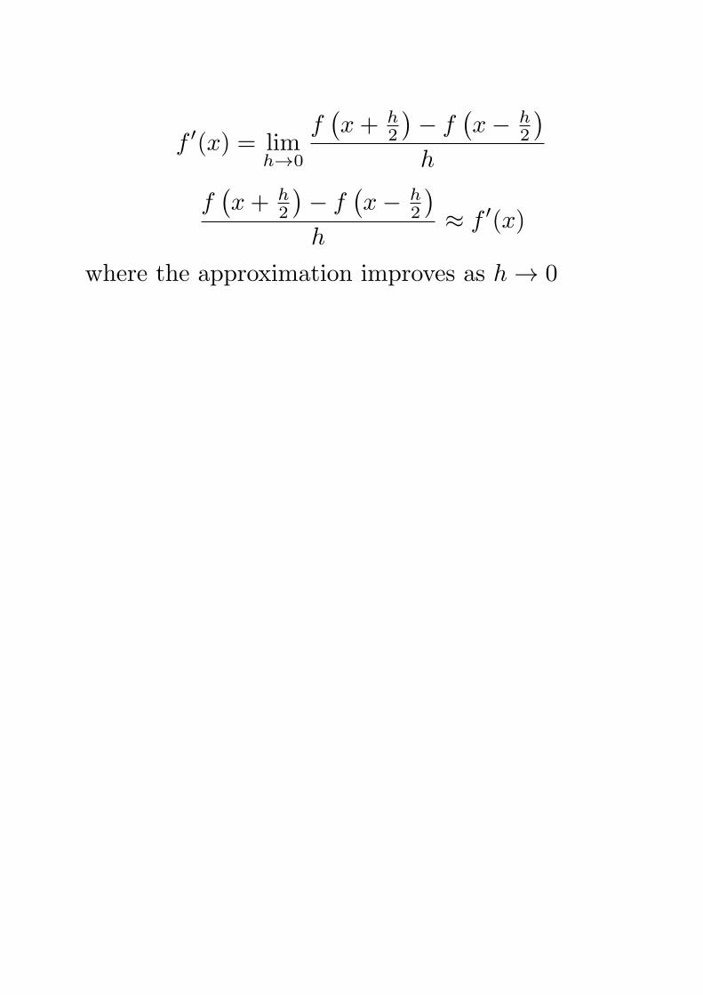
f ′(x) = limh→0
f(x+ h
2
)− f
(x− h
2
)h
f ′(x) = limh→0
f(x+ h
2
)− f
(x− h
2
)h
f(x+ h
2
)− f
(x− h
2
)h
≈ f ′(x)
where the approximation improves as h → 0
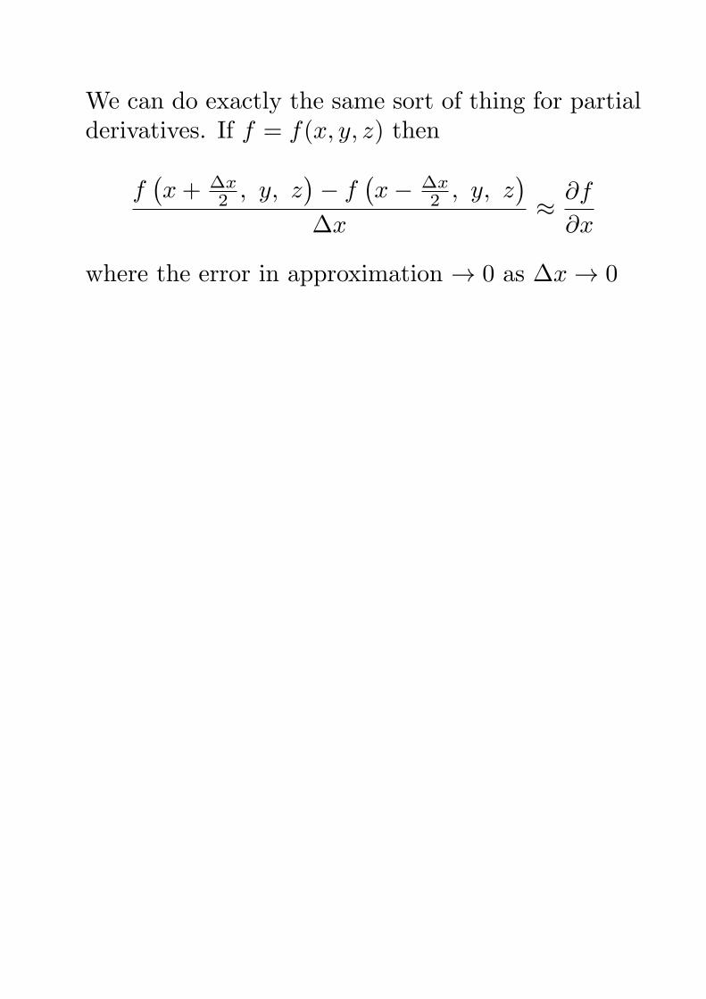
We can do exactly the same sort of thing for partialderivatives. If f = f(x, y, z) then
f(x+ ∆x
2 , y, z)− f
(x− ∆x
2 , y, z)
∆x≈ ∂f
∂x
where the error in approximation → 0 as ∆x → 0
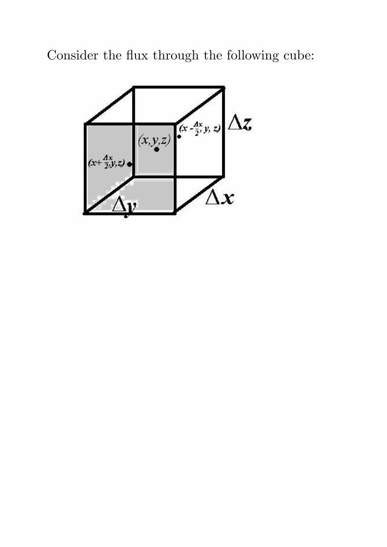
Consider the flux through the following cube:
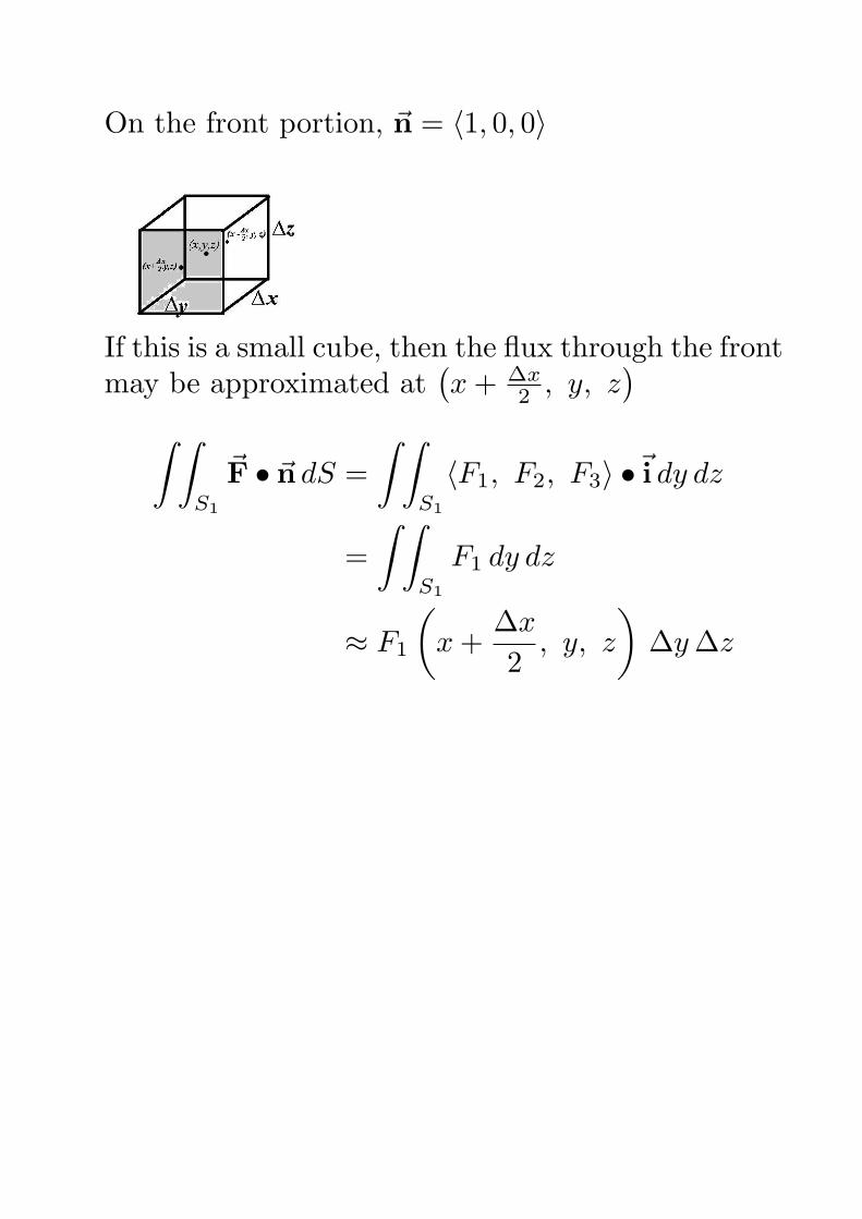
On the front portion, n⃗ = ⟨1, 0, 0⟩
If this is a small cube, then the flux through the frontmay be approximated at
(x+ ∆x
2 , y, z)
∫ ∫S1
F⃗ • n⃗ dS =
∫ ∫S1
⟨F1, F2, F3⟩ • i⃗ dy dz
=
∫ ∫S1
F1 dy dz
≈ F1
(x+
∆x
2, y, z
)∆y∆z
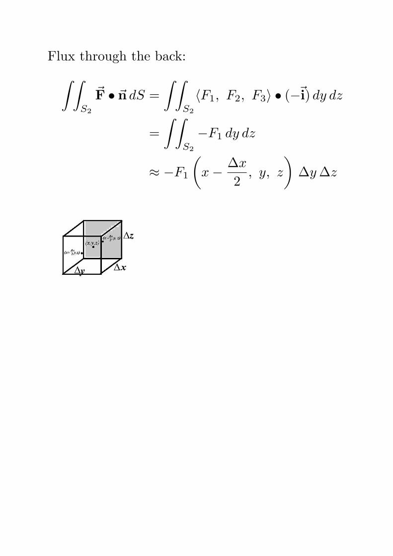
Flux through the back:∫ ∫S2
F⃗ • n⃗ dS =
∫ ∫S2
⟨F1, F2, F3⟩ • (−⃗i) dy dz
=
∫ ∫S2
−F1 dy dz
≈ −F1
(x− ∆x
2, y, z
)∆y∆z
Total approximate flux through the front and back:(F1
(x+ ∆x
2 , y, z)− F1
(x− ∆x
2 , y, z))
∆y∆z
Total approximate flux through the front and back:(F1
(x+ ∆x
2 , y, z)− F1
(x− ∆x
2 , y, z))
∆y∆z
This is equal to:
F1
(x+ ∆x
2 , y, z)− F1
(x− ∆x
2 , y, z)
∆x·∆x∆y∆z

Total approximate flux through the front and back:(F1
(x+ ∆x
2 , y, z)− F1
(x− ∆x
2 , y, z))
∆y∆z
This is equal to:
F1
(x+ ∆x
2 , y, z)− F1
(x− ∆x
2 , y, z)
∆x·∆x∆y∆z
This is approximately equal to:
∂F1
∂x(x, y, z)∆x∆y∆z
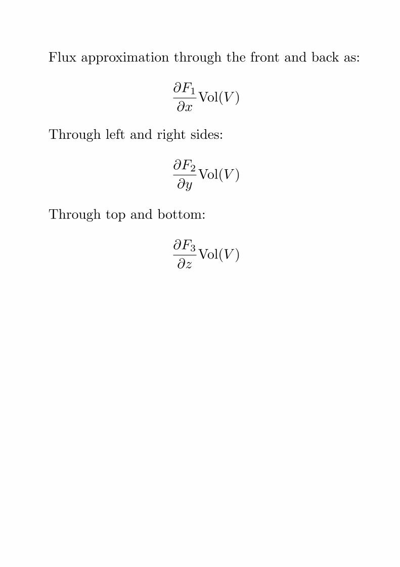
Flux approximation through the front and back as:
∂F1
∂xVol(V )
Flux approximation through the front and back as:
∂F1
∂xVol(V )
Through left and right sides:
∂F2
∂yVol(V )
Through top and bottom:
∂F3
∂zVol(V )
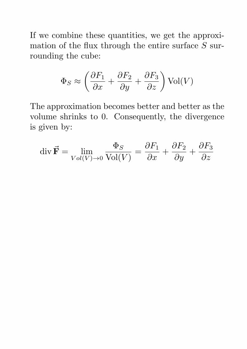
If we combine these quantities, we get the approxi-mation of the flux through the entire surface S sur-rounding the cube:
ΦS ≈(∂F1
∂x+
∂F2
∂y+
∂F3
∂z
)Vol(V )
The approximation becomes better and better as thevolume shrinks to 0. Consequently, the divergenceis given by:
div F⃗ = limV ol(V )→0
ΦS
Vol(V )=
∂F1
∂x+
∂F2
∂y+
∂F3
∂z
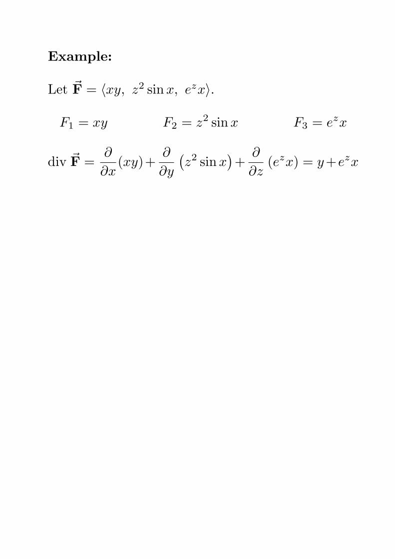
Example:
Let F⃗ = ⟨xy, z2 sinx, ezx⟩.
F1 = xy F2 = z2 sinx F3 = ezx
div F⃗ =∂
∂x(xy)+
∂
∂y
(z2 sinx
)+
∂
∂z(ezx) = y+ezx
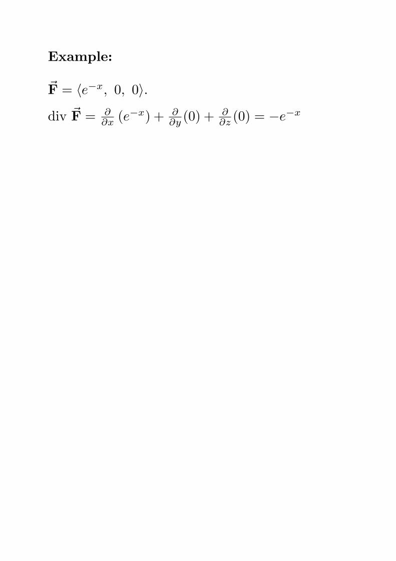
Example:
F⃗ = ⟨e−x, 0, 0⟩.
div F⃗ = ∂∂x (e−x) + ∂
∂y (0) +∂∂z (0) = −e−x
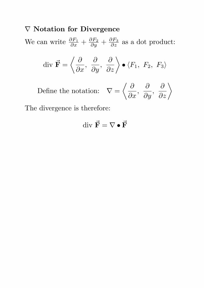
∇ Notation for Divergence
We can write ∂F1
∂x + ∂F2
∂y + ∂F3
∂z as a dot product:
div F⃗ =
⟨∂
∂x,
∂
∂y,
∂
∂z
⟩• ⟨F1, F2, F3⟩
Define the notation: ∇ =
⟨∂
∂x,
∂
∂y,
∂
∂z
⟩The divergence is therefore:
div F⃗ = ∇ • F⃗
Recall that the derivative f ′(x) can be written asDf . Compare the derivative of a function Df to thedivergence ∇ • F⃗.
Product Rule:
D(fg) = fDg + gDf
If ϕ(x, y, z) is a scalar-valued function and
F⃗ = ⟨F1(x, y, z), F2(x, y, z), F3(x, y, z)⟩ is a vector
field then ϕF⃗ is also a vector field (a scalar times avector) and its divergence is:
div(ϕF⃗) = ∇ • (ϕF⃗)
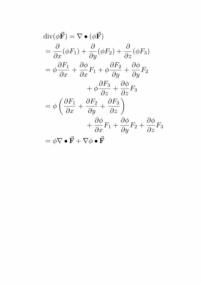
div(ϕF⃗) = ∇ • (ϕF⃗)
=∂
∂x(ϕF1) +
∂
∂y(ϕF2) +
∂
∂z(ϕF3)
= ϕ∂F1
∂x+
∂ϕ
∂xF1 + ϕ
∂F2
∂y+
∂ϕ
∂yF2
+ ϕ∂F3
∂z+
∂ϕ
∂zF3
= ϕ
(∂F1
∂x+
∂F2
∂y+
∂F3
∂z
)+
∂ϕ
∂xF1 +
∂ϕ
∂yF2 +
∂ϕ
∂zF3
= ϕ∇ • F⃗+∇ϕ • F⃗
Compare D(fg) = fDg + gDf to
∇ • (ϕF⃗) = ϕ∇ • F⃗+∇ϕ • F⃗

∇ • (ϕF⃗) = ϕ∇ • F⃗+∇ϕ • F⃗
Special Case:
Suppose the scalar ϕ is a constant C.
∇ϕ =⟨
∂∂x (C), ∂
∂y (C), ∂∂x (C),
⟩= ⟨0, 0, 0⟩ = 0⃗
div(CF⃗) = C∇ • F +∇C • F⃗
= C∇ • F + 0⃗ • F⃗= C∇ • F
= C div F⃗
A fluid is incompressible if the density remains con-stant. If ρ is the constant density and v⃗ is the ve-locity vector field of the fluid, and F⃗ = ρv⃗ then
div F⃗ = −∂ρ
∂t
div(ρv⃗) = − ∂
∂t(constant) = 0
ρdiv v⃗ = 0
Dividing both sides by ρ leaves us with:
div v⃗ = 0
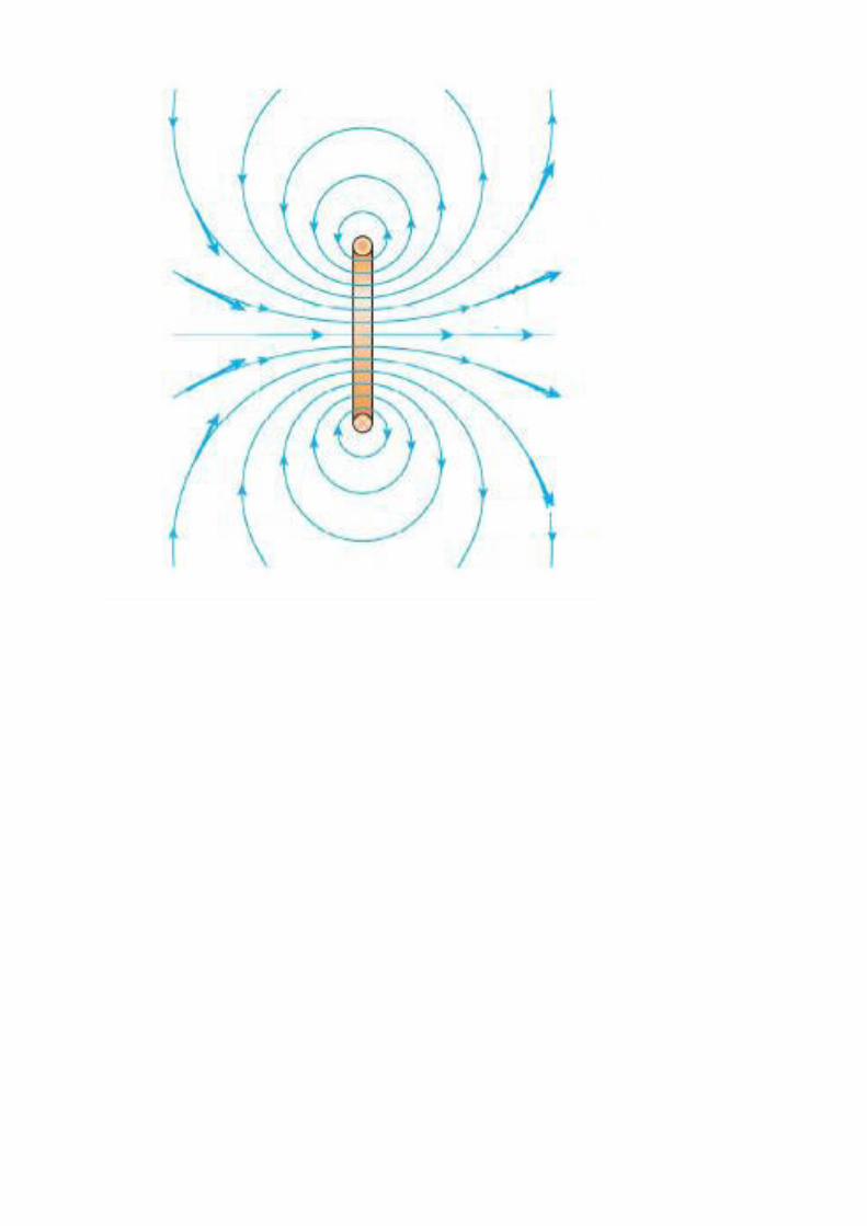
Application to Magnetic Fields
Consider the magnetic field B⃗.

Let’s take some arbitrary point (x, y, z) and con-struct a closed surface around it.
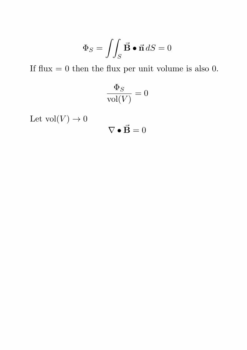
Gauss’s Law for Magnetism:
ΦS =
∫ ∫S
B⃗ • n⃗ dS = 0
ΦS =
∫ ∫S
B⃗ • n⃗ dS = 0
If flux = 0 then the flux per unit volume is also 0.
ΦS
vol(V )= 0
Let vol(V ) → 0
∇ • B⃗ = 0
∫ ∫S
B⃗ • n⃗ dS = 0
∇ • B⃗ = 0