Title Analysis of Car-following Behavior on Sag and …...Analysis of Car-following Behavior on Sag and Curve Sections at Intercity Expressways with Driving Simulator Ryuji Yoshizawa*1

Title Analysis of Car-following Behavior on Sag and Curve Sectionsat Intercity Expressways with Driving Simulator

Author(s) Yoshizawa, Ryuji; Shiomi, Yasuhiro; Uno, Nobuhiro; Iida,Katsuhiro; Yamaguchi, Masao

Citation International Journal of Intelligent Transportation SystemsResearch (2012), 10(2): 56-65

Issue Date 2012-05

URL http://hdl.handle.net/2433/155092

Right

The final publication is available at www.springerlink.com; この論文は出版社版でありません。引用の際には出版社版をご確認ご利用ください。This is not the published version.Please cite only the published version.

Type Journal Article

Textversion author

Kyoto University

Analysis of Car-following Behavior on Sag and Curve Sections at

Intercity Expressways with Driving Simulator

Ryuji Yoshizawa*1

Yasuhiro Shiomi*1

Nobuhiro Uno*2

Katsuhiro Iida*3

Masao Yamaguchi*3

Graduate School of Engineering, Kyoto University*1

(C-1-2, Kyoto University Katsura, Nishikyo-ku, Kyoto, 615-8540, Japan, +81-75-383-3235,

[email protected])

Graduate School of Management, Kyoto University*3

(C-1-2, Kyoto University Katsura, Nishikyo-ku, Kyoto, 615-8540, Japan, +81-75-383-3234,

[email protected])

Graduate School of Engineering, Osaka University*3

(2-1, Yamadagaoka, Suita city,Osaka, 565-0871, Japan, +81-6-6879-7611,

[email protected])

We analyzed the influence of road alignments such as sags and curves and the leading vehicle’s behavior on car-

following behavior in a driving simulator experiment. Parameters of a car-following model were estimated from

following-vehicle trajectory data collected for 37 participants. Then, relationships between the parameters and

environmental factors were analyzed. The results showed that the parameters of the following-behavior model were

significantly influenced by expressway alignments such as sags and curves, whereas differences in the leading vehicle’s

behavior did not significantly affect the estimated parameters. These findings indicate that measures to assist the

following vehicle’s acceleration and deceleration such as adaptive cruise control could be effective in preventing the

breakdown of traffic flow.

Key words: car-following behavior, driving simulator, road alignment, in-laboratory experiment

1. Introduction

Some sections of Japanese freeways, including sags

and tunnel entrances without any lane drops, merging, or

diverging, become bottlenecks and congestion queues

often appear behind these sections [1]. Sag bottlenecks

are major causes of traffic congestion on Japanese

freeways. Furthermore, the risk of traffic accidents is

much higher in congested traffic state than in free flow

state [2]. Too enhance both efficiency and safety,

measures to prevent traffic breakdown and to mitigate

traffic congestion at sag bottlenecks are needed. To do

so, precise understanding of such bottleneck phenomena

is required.

Many attempts to understand the mechanisms of

traffic breakdown and queue formation on basic sections

of freeways, including sags and tunnels, have been made

since Koshi et al. [3] noted that bottlenecks could form

along basic sections of freeway. For example, Koshi [4]

hypothesized that speed reduction occurred at sag

sections. On the basis of this hypothesis, car-following

behavior models of speed reduction and queue formation

on sag sections were developed and calibrated,

considering the influence of longitudinal gradient [5][6].

Although many types of car-following model have been

proposed, the question of why traffic breakdown occurs

at specific sags and tunnels remains unresolved [7].

Oguchi suggested several conditions of sags where

could be bottlenecks, based on empirical observation

data at 36 sags on Japanese freeways [8]. In terms of

driving and car-following behavior, however, the

detailed mechanisms of traffic breakdown are unclear,

largely because of the difficulty of observing traffic flow

and collecting traffic trajectory data under the same

condition. That is, driving behavior can be influenced by

many factors such as weather [9], sunshine [10], and

surrounding traffic conditions, which cannot be

managed by observers. In addition, driving and car-

following behaviors vary widely among vehicles,

depending on the roadway section [11] [12], and thus it is

difficult to specify the true influence of sags on car-

following behavior.

On the other hand, advances in information

technology have allowed for experimental approaches

using driving simulators (e.g., Hoogendoorn et al. [13],

Rong et al. [14], Yang et al. [15]). If verified to be realistic,

driving simulators can be useful for analyzing sag

bottleneck phenomena. In a virtual reality environment,

operators can manage all factors affecting car-following

behavior, allowing the true influence of sags on car-

following behaviors to be isolated and observed.

Regarding sag bottlenecks, Oguchi and Iida showed that

traffic congestion at sag bottlenecks could be

represented in a car-following experiment using a

driving simulator [16]. Their result supports the

applicability of using driving simulators to analyze sag

bottleneck phenomena.

In this study, we used the well-calibrated driving

simulator developed by Oguchi and Iida [16] to

investigate the influence of freeway alignments on car-

following behavior in an in-laboratory experiment.

Concretely, we considered freeway alignments,

including two types of sags and two types of curve

sections, and two types of leading vehicle movement.

Data on car-following and driving behavior were

collected from 37 participants and analyzed with respect

to each alignment and lead vehicle movement using

statistical approaches. Finally, the mechanisms of speed

reduction at specific types of sags are discussed.

Section 2 describes the design of the laboratory

experiment using the driving simulator. In Section 3, the

characteristics of driving behavior with respect to each

road alignment and lead vehicle movement are analyzed

focusing on the longitudinal change in the speed of

following vehicles and accelerator opening degrees.

Section 4 presents the estimated parameters of the car-

following model, and the differences in the parameters

with respect to road alignments and lead vehicle

movements are verified by applying analysis of variance

(ANOVA) and multiple comparisons. Finally, we

discuss the speed reduction mechanism and measures to

prevent traffic breakdown.

2. Experimental design

2.1. Architecture of the driving simulator

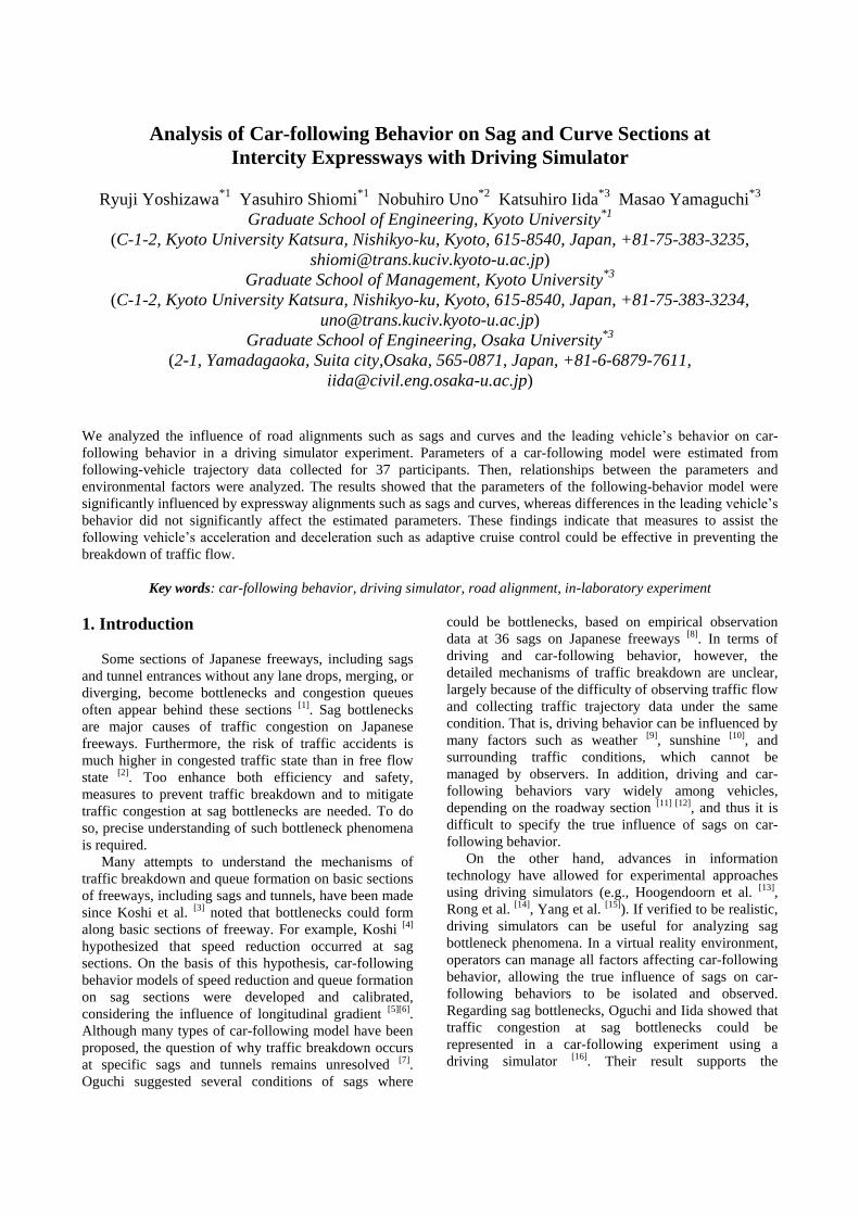
The driving simulator used in this study was

developed by Oguchi and Iida [16]. Figure 1 shows the

architecture of the simulator, which consists of a central

processing unit, a visual generation system, a 3D sound

system, and an automatic transmission driving operation

unit that is a recreation of a real automatic transmission

car with a speedometer. Although motion systems, such

as vibration generators, were not built into the simulator,

visual and acoustic features provide the driver with a

sense of speed and acceleration.

Calibration and validation of a driving simulator are

important for ensuring the accuracy and reliability of the

simulated results. The simulator used in this study has

been rigorously calibrated and validated since 1998 in

terms of longitudinal change in driving speed and

accelerator opening degree [17]. In particular, the

reproducibility of the sag bottleneck phenomenon was

verified [16]. Thus, we considered this simulator to be

sufficiently accurate and reliable for analyzing car-

following behavior.

2.2. Design of freeway alignments To investigate difference in car-following behavior with

respect to freeway alignments, five types of driving

courses were prepared: courses with (i) a gentle curve

section, (ii) a sharp curve section, (iii) a gentle sag

section, (iv) a sharp sag section, and (v) a normal

straight section. Table 1 summarizes the freeway

features of the experimental driving courses. In each

driving course, certain points were indicated by

kilometer posts (kp) from the origin point. For example,

in the gentle curve course, the experiment started at

2.5 kp and ended at 4.5 kp; a participant drove the 2.0-

km distance, within which the driving data collected

from 3.2 to 4.2 kp were used for the analysis. Note that

the sharp curve feature and the straight feature were

included in the same course. Each course consisted of

two lanes in one direction, and the lead and following

vehicle were assumed to drive in the inner lane.

2.3. Lead vehicle movements Lead vehicle movements can significantly affect the

driving and car-following behavior of the following

vehicle. For example, we can consider two possible

reasons for deceleration of the following vehicle at a sag

section: reaction to considerable deceleration of the lead

vehicle and insufficient acceleration against the

deceleration caused by the road alignment. It is

necessary to separate these two influences on the

following vehicle to clarify the influence of the freeway

alignments.

Thus, we prepared two movement patterns for the

lead vehicle: in one, a constant speed (95 km/h) was

Driving operation unit

3D sound systemCPU Visual generation system

Flow of data

Figure 1. Architecture of the driving simulator

Table 1. Freeway alignments of each course

From To From To

Gentle curve

Curvature radius: 800 m

Longitudial gradient: + 0.5%

Curve section: from 3.2 kp to 4.1 kp

2.5 kp 4.5 kp 3.2 kp 4.2 kp

Sharp curve

Curvature radius: 400 m

Longitudial gradient: - 0.5%

Curve section: from 8.9 kp to 9.7 kp

7.8 kp 12.0 kp 8.8 kp 9.8 kp

Gentle sag

Curvature radius: 1,000 m

Longitudial gradient: - 1.9% to + 1.6 %

Bottom of sag: from 62.1 kp to 62.0 kp

63.2 kp 60.6 kp 62.5 kp 61.3 kp

Sharp curve

Curvature radius: 1,000 m

Longitudial gradient: - 1.9% to + 5.0 %

Bottom of sag: from 62.1 kp to 62.0 kp

63.2 kp 60.6 kp 62.5 kp 61.3 kp

StraightCurvature radius: 4,000 m

Longitudial gradient: - 2.5%7.8 kp 12.0 kp 8.2 kp 8.8 kp

Course Alignments of target sectionDriving course interval Target section interval

International Journal of ITS Research, Vol. 1, No. 1, December 2003

maintained despite the road alignments (“constant case”),

and in the other driving speed varied “naturally” in

accordance with the freeway alignments (“natural case”).

For the natural case, we generated a driving profile of

the lead vehicle by operating the driving simulator on

the basis of a speed-profile model of the relationship

between free-flow speed and roadway alignments [18]. In

the speed-profile model, the basic speed was set as 100

km/h. On sag and curved sections, the lead vehicle speed

became around 95 km/h, which is the same as the speed

in the constant case.

2.4. Design of traffic conditions To produce as realistic a driving situation as possible,

surrounding vehicles were allocated around the lead and

following vehicles. Several vehicles were located in

front of the lead vehicle and behind the following

vehicle, from 250 m apart, so as not to influence on the

following vehicle’s driving behavior. Additionally, in

the shoulder lane, other vehicles were allocated

alongside for the whole course; the vehicles maintained

distances of 70 m from each other and moved at 90 km/h,

to simulate a relatively congested traffic situation. In the

inner lane, all vehicles including the lead and following

vehicles were passenger cars, whereas in the outer lane

30% of the vehicles were trucks.

2.5. Participants and procedures All participants were randomly selected from

university students with a valid driver license. Thirty-

seven drivers (27 males, 10 females) participated in the

experiment. The participants ranged from 21 to 26 years

of age, with a mean of 23.4 years (SD = 1.32). Driving

experience varied from 1 month to 6 years, with a mean

of 2.99 years (SD = 1.66).

Each driver was instructed to follow the lead vehicle

in eight experimental cases, consisting of two cases for

the movement of the lead vehicle in each of the four

driving courses. The order of the eight cases was

randomized to eliminate any order effect. That is, all the

participants completed the cases in a different order.

Before the experiment, each participant had 20 min to

drive and become accustomed to the simulator. All

participants received monetary compensation for their

participation in the experiment.

3. Fundamental analysis of driving behavior

This section overviews the differences in driving and

car-following behavior by case based on longitudinal

changes in driving speed and accelerator opening

degrees of the following vehicle.

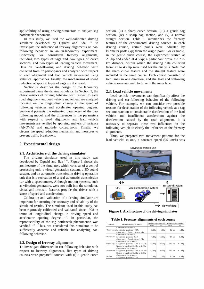
3.1. Longitudinal change in driving speed Figures 2, 3, 4, and 5 show the longitudinal change in

average driving speed of all participants for the gentle

sag section, sharp sag section, gentle curve section, and

sharp curve section, respectively. In the figures, the

longitudinal changes in lead vehicle speed, and the

changes in altitude for inclined sections and curvature

radii for curved sections, are also illustrated.

For both sag sections, the points where the average

speed is lowest tend to be located more downstream in

the natural case, where a lead vehicle varies its driving

speed according to the road alignments, than in the

constant case, where the lead vehicle maintains a

constant speed despite road alignment. That is, in the

constant case, the following vehicles accelerate earlier

than in the natural case. This indicates that when the lead

vehicle maintains its speed throughout the whole section,

the driver of the following vehicle notices the speed gap

at an earlier stage and thus can recover speed before a

large speed reduction occurs.

355

360

365

370

375

380

385

390

395

400

405

80

85

90

95

100

105

110

60.961.161.361.561.761.962.162.362.5A

ltit

ud

e （

m）

Ave

rage

sp

ee

d （

km/h）

KP

Lead vehicle speed (constant case)

Average speed of following vehicles (constant case)

Lead vehicle speed (natural case)

Average speed of following vehicles (natural case)

Altitude

Moving direction

The lowest speed point

The lowest speed point

Figure 2. Longitudinal speed changes

on the gentle sag section.

355

360

365

370

375

380

385

390

395

400

405

80

85

90

95

100

105

110

60.961.161.361.561.761.962.162.362.5

Alt

itu

de

（m）

Ave

rage

sp

ee

d（

km/h）

KP

Lead vehicle speed (constant case)Average speed of following vehicles (constant case)Lead vehicle speed (natural case)Average speed of following vehicles (natural case)Altitude

Moving direction

The lowest speed pointThe lowest speed point


on the sharp sag section.

In contrast, the tendency is different in the curve

sections. From Figures 4 and 5, it can be seen that the

points where the following vehicles take the lowest

speed are almost same regardless of the lead vehicle

movement. It must be because in the curve section the

influence of the road alignment on the driving behavior

is more significant than of the lead vehicle movement.

The driver should operate the handle as well as the

accelerator to follow the lane safely. This tendency is

confirmed by the fact that on the gently curved section,

the driving speed gradually decreased as the curvature

radius decreased, whereas on the sharp curve section,

driving speed decreased suddenly with the sudden

reduction in the curvature radius.

3.2. Longitudinal change in accelerator opening

degrees To further analyze the driving behavior of the

following vehicle, the accelerator opening degree was

analyzed. This measure was defined in the interval from

0% to 100% in the angle of the accelerator pedal

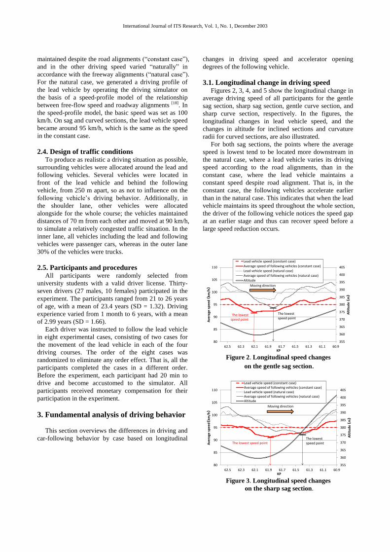
position. Figures 6, 7, and 8 summarize the longitudinal

changes in the average of the accelerator opening degree

on the sag sections, on the gently curved section, and on

the sharply curved section, respectively.

Figure 6 shows that after taking the lowest value

around 62.4 kp, the accelerator opening degree increased,

from 62.2 kp to 61.5 kp, at almost the same rate

regardless of road alignments or lead vehicle movement.

On the gentle sag section, the opening degree increased

to 45%, while on the sharp sag section it increased to

50% or 55%. These results indicate that the accelerator

opening degree needed to increase the driving speed

differs depending on the gradient of the incline. When

20

25

30

35

40

45

50

55

60

60.961.161.361.561.761.962.162.362.5

Acc

eler

ato

r o

pen

ing

deg

rees

（%）

KP

Gentle sag/ constant case Gentle sag/ natural case

Sharp sag/ constant case Sharp sag/ natural case

Moving direction

Altitude of the sharp sag

Altitude of the gentle sag

Figure 6. Longitudinal change in accelerator opening

degree on sag sections.

0

500

1000

1500

2000

2500

3000

3500

4000

4500

20

30

40

50

60

3 3.2 3.4 3.6 3.8 4 4.2

Cu

rvat

ure

rad

ius

(m)

Acc

ele

rato

r o

pe

nin

g d

egr

ee

(%

)

KP

Constant case Natural case Curvature radius

Moving direction


degree on the gentle curve section.

0

500

1000

1500

2000

2500

3000

3500

4000

4500

20

30

40

50

60

8.8 9 9.2 9.4 9.6 9.8 10

Cu

rvat

ure

rad

ius

(m)

Acc

ele

rato

r o

pe

nin

g d

egr

ee

(%

)

KP

Constant case Natural case Curvature radius

Moving direction


degree on sharp curve section.

0

500

1000

1500

2000

2500

3000

3500

4000

4500

80

85

90

95

100

105

110

3 3.2 3.4 3.6 3.8 4 4.2

Cu

rvat

ure

rad

ius （

m）

Ave

rage

sp

ee

d (

km/h

)

KP

Lead vehicle speed (constant case)

Average speed of following vehicles (constant case)

Lead vehicle speed (natural case)

Average speed of following vehicles (natural case)

Curvature radius

Moving direction

The lowest point

The lowest point


on the gentle curve section.

0

500

1000

1500

2000

2500

3000

3500

4000

4500

80

85

90

95

100

105

110

8.8 9 9.2 9.4 9.6 9.8 10

Cu

rvat

ure

rad

ius（

m）

Ave

rage

sp

ee

d (

km/h

)

KP

Lead vehicle speed (natural case)Average speed of following vehicles (constant case)Lead vehicle speed (constant case)Average speed of following vehicles (natural case)Curvature radius

Moving direction

The lowest pointThe lowest point


on the sharp curve section.


the upgrade is steeper, it takes more time to open the

accelerator to a sufficient degree to increase the speed.

Thus, on the sharp sag section, the points where the

driving speed was lowest were located farther

downstream than in the gentle sag section.

On the curved section, the opening degree decreased

in the section where the curvature radius decreased, as

shown in Figures 7 and 8, and after the radius became

stable, the degree of opening tended to increase. This

tendency was observed in both the constant and natural

cases. This result is consistent with the longitudinal

speed changes shown in Figures 4 and 5. Thus, speed

reduction on the curved section was apparently caused

primarily by the driver's behavior in response to the

change in the radius of curvature.

4. Analysis of parameters of car-following

models

Analysis of the accelerator opening degree reveals the

influence of road alignments on car-following and

driving behaviors. To investigate the influence of road

alignments in terms of car-following behavior, the

parameters of car-following models were estimated and

the relationship between parameters and road alignments

was investigated.

4.1. Estimation of car-following model

parameters Parameters were estimated with respect to each pair

of trajectories of the lead vehicle and following vehicle.

The experiments involved two cases of lead vehicle

movements with respect to five target sections for 37

participants; thus, in total 370 (2 cases × 5 sections ×

37 participants) sets of parameters could be estimated.

Data about acceleration, speed, and coordinates of each

vehicle required for the parameter estimation were

collected every 0.1 s. The estimated parameters were

analyzed by applying ANOVA in which the movements

of the lead vehicle and road alignments were considered

as explanatory variables.

4.1.1. Choice of car-following model. Among

numerous car-following models, the Helley model [19]

expressed in Eq. (1) was chosen. This model assumes a

linear relationship between the acceleration and the

relative speed and headway distance, and allows for

straightforward interpretation of the estimated

parameters. Note that this study aims for understanding

the influence of road alignments on car-following

behavior, instead of establishing a car-following model

considering the influence of road alignments.

31021011 )()()()( atxtxatxtxattx , (1)

where

txi : the acceleration of vehicle i at time t,

txi : the speed of vehicle i at time t,

txi : the coordinate of vehicle i exists at time t,

i: 0 indicates a lead vehicle and 1 indicates a

following vehicle,

t: reaction time and

a1, a2, a3: estimation parameters.

In Eq. (1), the constant value a3 can be included in the

second term of the right side as follows:

dtxtxatxtxa

a

atxtxatxtxattx

)()()()(

)()()()(

102101

2

31021011

(2)

where d (= -a3/a2) indicates the desired gap between

the lead vehicle and following vehicle.

Parameters were estimated by applying the least-

squares method with t changing from 0.1 s to 3.0 s by

0.1 s. Among the various t, the value at which the

adjusted R2 is maximized was determined as the

estimated reaction time. Note that the reaction time was

estimated for each trial, and thus, the estimated reaction

time may vary even within the same participant's data.

4.1.2. Conditions of the following behavior. Although

participants were instructed to follow the lead vehicle,

there were some participants who did not catch up with

the lead vehicle and, as a result, could not follow it. In

such cases, the estimated parameters of the Helley model

do not have significant meanings. The following four

criteria were considered, and data that did not satisfy the

criteria were eliminated.

Criterion 1: The following vehicle maintains less than

3.0 s headway to the lead vehicle for 5.0 s or more.

Criterion 2: The time-series change in the relative speed

between the lead vehicle and the following vehicle is

neither monotone decreasing nor monotone increasing.

Criterion 3: The coefficient of determinant of the

parameter estimation is 0.3 or more.

Criterion 4: The correlation coefficient between the

relative speed and the headway distance, which are both

explanatory variables in the Helley model in Eq. (1), is

less than 0.9.

Criterion 1 was intended to eliminate drivers who did

not follow the lead vehicle because of insufficient

acceleration. In Criterion 2, monotone increase in

relative speed represents a situation in which the

following vehicle is being left behind by the lead vehicle.

Monotone decrease corresponds to the situation in which

the following vehicle is just catching up with the lead

vehicle. These situations were irrelevant to the focus of

the present analysis. Criterion 3 removes drivers whose

following behaviors do not fit the Helley model, and

Criterion 4 indicates the general condition to check for

multicollinearity in the regression analysis. After

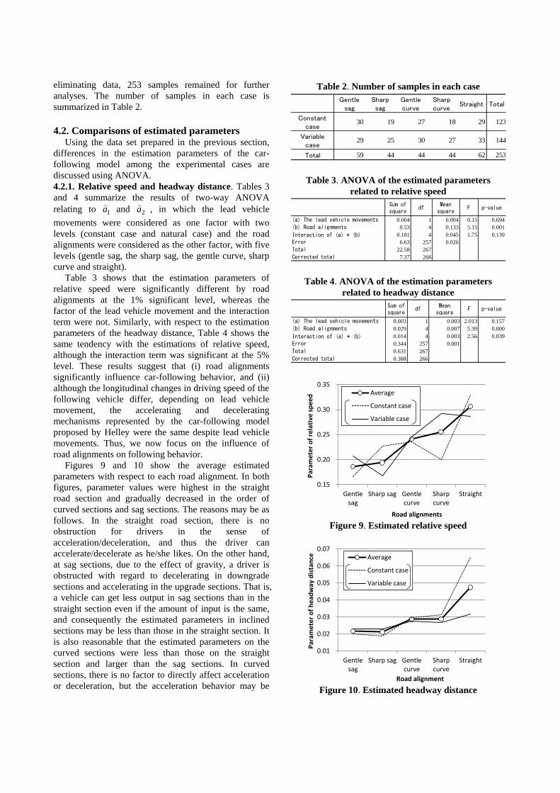
eliminating data, 253 samples remained for further

analyses. The number of samples in each case is

summarized in Table 2.

4.2. Comparisons of estimated parameters Using the data set prepared in the previous section,

differences in the estimation parameters of the car-

following model among the experimental cases are

discussed using ANOVA.

4.2.1. Relative speed and headway distance. Tables 3

and 4 summarize the results of two-way ANOVA

relating to 1a

and 2a

, in which the lead vehicle

movements were considered as one factor with two

levels (constant case and natural case) and the road

alignments were considered as the other factor, with five

levels (gentle sag, the sharp sag, the gentle curve, sharp

curve and straight).

Table 3 shows that the estimation parameters of

relative speed were significantly different by road

alignments at the 1% significant level, whereas the

factor of the lead vehicle movement and the interaction

term were not. Similarly, with respect to the estimation

parameters of the headway distance, Table 4 shows the

same tendency with the estimations of relative speed,

although the interaction term was significant at the 5%

level. These results suggest that (i) road alignments

significantly influence car-following behavior, and (ii)

although the longitudinal changes in driving speed of the

following vehicle differ, depending on lead vehicle

movement, the accelerating and decelerating

mechanisms represented by the car-following model

proposed by Helley were the same despite lead vehicle

movements. Thus, we now focus on the influence of

road alignments on following behavior.

Figures 9 and 10 show the average estimated

parameters with respect to each road alignment. In both

figures, parameter values were highest in the straight

road section and gradually decreased in the order of

curved sections and sag sections. The reasons may be as

follows. In the straight road section, there is no

obstruction for drivers in the sense of

acceleration/deceleration, and thus the driver can

accelerate/decelerate as he/she likes. On the other hand,

at sag sections, due to the effect of gravity, a driver is

obstructed with regard to decelerating in downgrade

sections and accelerating in the upgrade sections. That is,

a vehicle can get less output in sag sections than in the

straight section even if the amount of input is the same,

and consequently the estimated parameters in inclined

sections may be less than those in the straight section. It

is also reasonable that the estimated parameters on the

curved sections were less than those on the straight

section and larger than the sag sections. In curved

sections, there is no factor to directly affect acceleration

or deceleration, but the acceleration behavior may be

Table 2. Number of samples in each case

Gentlesag

Sharpsag

Gentlecurve

Sharpcurve

Straight Total

Constantcase

30 19 27 18 29 123

Variablecase

29 25 30 27 33 144

Total 59 44 44 44 62 253

Table 3. ANOVA of the estimated parameters

related to relative speed

Sum ofsquare

dfMeansquare

F p-value

(a) The lead vehicle movements 0.004 1 0.004 0.15 0.694

(b) Road alignments 0.53 4 0.133 5.15 0.001

Interaction of (a) * (b) 0.181 4 0.045 1.75 0.139

Error 6.63 257 0.026

Total 22.58 267

Corrected total 7.37 266

Table 4. ANOVA of the estimation parameters

related to headway distance

Sum ofsquare

dfMeansquare

F p-value




Error 0.344 257 0.001

Total 0.631 267


0.15

0.20

0.25

0.30

0.35

Gentlesag

Sharp sag Gentlecurve

Sharpcurve

Straight

Par

ame

ter

of

rela

tive

sp

eed

Road alignments

Average

Constant case

Variable case

Figure 9. Estimated relative speed

0.01

0.02

0.03

0.04

0.05

0.06

0.07

Gentlesag


Sharpcurve

Straight

Par

ame

ter

of

hea

dw

ay d

ista

nce

Road alignment

Average

Constant case

Variable case

Figure 10. Estimated headway distance


significantly influenced by adjusting the steering wheel

and accelerator pedal to follow the lane safely.

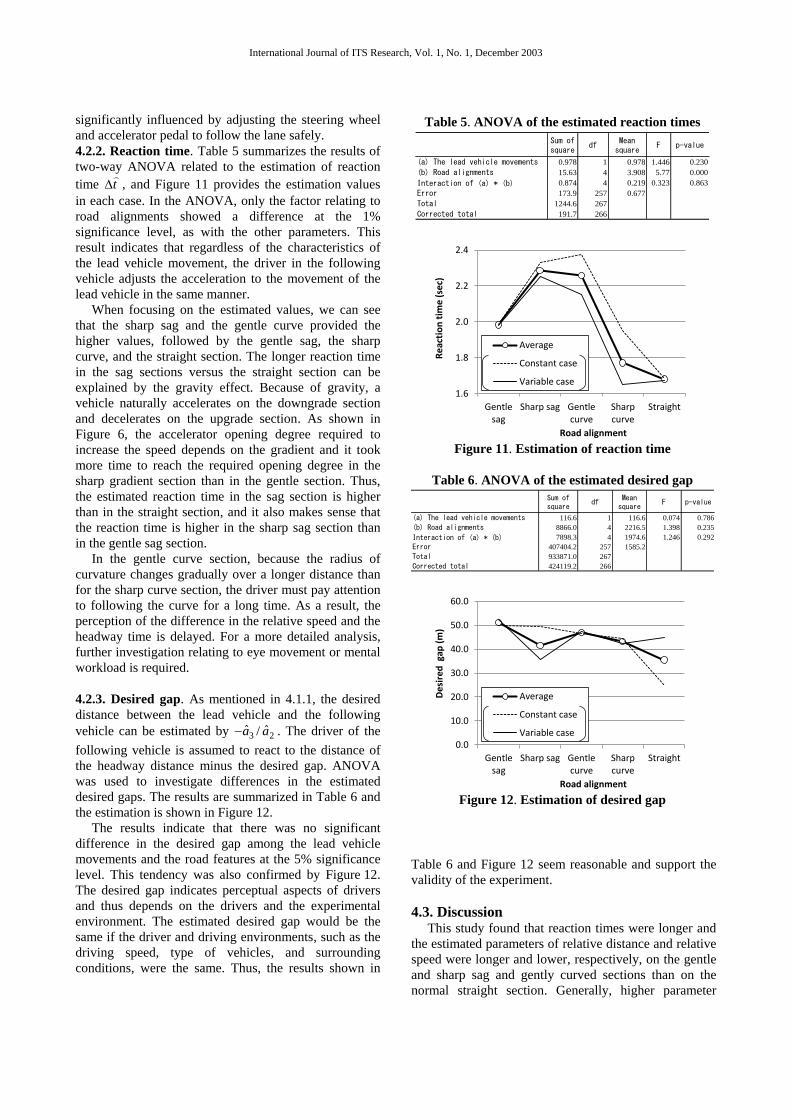
4.2.2. Reaction time. Table 5 summarizes the results of

two-way ANOVA related to the estimation of reaction

time t

, and Figure 11 provides the estimation values

in each case. In the ANOVA, only the factor relating to

road alignments showed a difference at the 1%

significance level, as with the other parameters. This

result indicates that regardless of the characteristics of

the lead vehicle movement, the driver in the following

vehicle adjusts the acceleration to the movement of the

lead vehicle in the same manner.

When focusing on the estimated values, we can see

that the sharp sag and the gentle curve provided the

higher values, followed by the gentle sag, the sharp

curve, and the straight section. The longer reaction time

in the sag sections versus the straight section can be

explained by the gravity effect. Because of gravity, a

vehicle naturally accelerates on the downgrade section

and decelerates on the upgrade section. As shown in

Figure 6, the accelerator opening degree required to

increase the speed depends on the gradient and it took

more time to reach the required opening degree in the

sharp gradient section than in the gentle section. Thus,

the estimated reaction time in the sag section is higher

than in the straight section, and it also makes sense that

the reaction time is higher in the sharp sag section than

in the gentle sag section.

In the gentle curve section, because the radius of

curvature changes gradually over a longer distance than

for the sharp curve section, the driver must pay attention

to following the curve for a long time. As a result, the

perception of the difference in the relative speed and the

headway time is delayed. For a more detailed analysis,

further investigation relating to eye movement or mental

workload is required.

4.2.3. Desired gap. As mentioned in 4.1.1, the desired

distance between the lead vehicle and the following

vehicle can be estimated by 3a / 2a . The driver of the

following vehicle is assumed to react to the distance of

the headway distance minus the desired gap. ANOVA

was used to investigate differences in the estimated

desired gaps. The results are summarized in Table 6 and

the estimation is shown in Figure 12.

The results indicate that there was no significant

difference in the desired gap among the lead vehicle

movements and the road features at the 5% significance

level. This tendency was also confirmed by Figure 12.

The desired gap indicates perceptual aspects of drivers

and thus depends on the drivers and the experimental

environment. The estimated desired gap would be the

same if the driver and driving environments, such as the

driving speed, type of vehicles, and surrounding

conditions, were the same. Thus, the results shown in

Table 6 and Figure 12 seem reasonable and support the

validity of the experiment.

4.3. Discussion

This study found that reaction times were longer and

the estimated parameters of relative distance and relative

speed were longer and lower, respectively, on the gentle

and sharp sag and gently curved sections than on the

normal straight section. Generally, higher parameter

Table 5. ANOVA of the estimated reaction times

Sum ofsquare

dfMeansquare

F p-value




Error 173.9 257 0.677

Total 1244.6 267


1.6

1.8

2.0

2.2

2.4

Gentlesag


Sharpcurve

Straight

Re

acti

on

tim

e (

sec)

Road alignment

Average

Constant case

Variable case

Figure 11. Estimation of reaction time

Table 6. ANOVA of the estimated desired gap

Sum ofsquare

dfMeansquare

F p-value




Error 407404.2 257 1585.2

Total 933871.0 267


0.0

10.0

20.0

30.0

40.0

50.0

60.0

Gentlesag


Sharpcurve

Straight

De

sire

d g

ap(m

)

Road alignment

Average

Constant case

Variable case

Figure 12. Estimation of desired gap

values and reaction times indicate a lower stability of

car-following [20]. However, as long as local stability and

asymptotic stability are satisfied, when the lead vehicle

decelerates at the bottom of a sag section, the following

vehicle with smaller parameters and longer reaction time

would be likely to shorten the relative distance because

the following vehicle would take more time to decelerate

to the same speed as the lead vehicle. In turn, when the

lead vehicle accelerates after passing through the bottom

of a sag section, a following vehicle with smaller

parameters and longer reaction time would take longer to

catch up with the lead vehicle. It would be why platoons

with high density are likely to be generated at the bottom

of sag sections, which have been found to induce speed

reduction and traffic breakdown [4][21]. Thus, in such a

section, a measure to prevent platoon formation would

be effective in preventing traffic breakdown and

mitigating traffic congestion. Based on the discussion,

reducing the reaction time and/or increasing the value of

car-following parameters would help mitigate bunching.

In this sense, adaptive cruise control to assist the

following vehicle’s acceleration and deceleration could

be a possible measure to help prevent traffic breakdown.

5. Conclusions

In the present study, we investigated the relationship

between car-following behavior and freeway alignments

by a laboratory experiment using a well-calibrated

driving simulator. In the experiment, five types of road

alignment were considered: gentle curve, sharp curve,

gentle sag, sharp sag, and straight section. The

movement of the lead vehicle was (i) kept at a constant

speed along with the whole course and (ii) varied

naturally according to the freeway alignments. In total,

37 participants took part in the experiment.

First, focusing on the longitudinal change in the

average speed and the average accelerator opening

degree for all participants, the influence of road features

on following behavior was examined. The data revealed

that in sag sections, the required accelerator opening

degree for acceleration varied depending on the upgrade

gradient and the target speed, which caused a delay in

recovering driving speed. At the beginning of a curve,

the following vehicle reduced the accelerator angle and

then tried to recover its speed again. In the recovering

period, the gradual changes in the radius of curvature

may have caused a delay in recovering the speed.

Then, the parameters of the car-following model were

estimated and analyzed in relation to freeway alignments.

This showed that (i) the parameters of the following

model varied significantly with respect to freeway

alignments, and (ii) differences in the movement of the

lead vehicle did not affect the estimated parameters.

Furthermore, in the sag section, the parameters of the

relative speed and headway distance tended to be lower

and the reaction time tended to be higher. This suggests

that when vehicles passed through s sag section,

headway distance between the successive vehicles was

likely to shorten and the accumulation of the vehicles

with the short headway distances possibly caused traffic

breakdown.

Some of the issues discussed here require further

analysis. For example, the quantitative relationship

between the freeway gradient and the required

accelerator opening degree for acceleration remains

unclear. The heterogeneity of driving behavior should

also be considered in future research. Moreover,

perception-reaction mechanisms and psychological

aspects are important in understanding bottleneck

phenomena on sag sections and in developing advanced

measures to prevent traffic breakdown, such as adaptive

cruise control and driver assist systems.

References

[1] Koshi, M., Kuwahara, M., Akahane, H., 1992.

Capacity of sags and tunnels in Japanese motorways.

ITE Journal, 17-22.

[2] Hikosaka, T., Nakamura, H., 2001. Statistical

analysis on the relationship between traffic accident rate

and traffic flow condition in basic expressway sections.

Proceedings of the 21st Japan Society of Traffic

Engineers (JSTE) Meeting, 173-176. (in Japanese).

[3] Koshi, M., Iwasaki, M., Ohkura, I., 1983. Some

findings and an overview on vehicular flow

characteristics. In: Hurdle, V. F., Hauer, E., Steuart, G.

N. (Eds.), Proceedings of the Eighth International

Symposium on Transportation and Traffic Theory,

University of Toronto Press, Toronto, 403-451.

[4] Koshi, M., 1986. Capacity of motorway bottlenecks.

Journal of the Japan Society of Civil Engineers 371(IV-

5), 1-7 (in Japanese).

[5] Ozaki, H., 1993. Reaction and anticipation in the car-

following behavior. Proceedings of 12th ISTTT

(Berkley), 349-366.

[6] Xing, J., Koshi, M., 1995. A study on the bottleneck

phenomena and car-following behavior on sags of

motorways. Journal of Infrastructure Planning and

Management 506 (IV-26), 45-55 (in Japanese).

[7] Oguchi, T., 2000. Analysis of bottleneck

phenomenon at a basic freeway segments – car

following model and future exploration –. Journal of

Infrastructure Planning and Management 660 (IV-49),

39-51. (in Japanese).

[8] Oguchi, T., 1995. Relationship between traffic

congestion phenomena and road alignments at sag

sections on motorways. Journal of Infrastructure

Planning and Management 524 (IV-29), 69-78. (in

Japanese).

[9] Chung, E., Ohtani, O., Warita, H., Kuwahara, M.,

Morita, H., 2006. Does weather affect highway

capacity? Proceedings of the 5th TRB International


Symposium on Highway Capacity and Quality of

Service,

[10] Kusakabe, T., Iryo, T., Asakura, Y., 2010. Data

mining for traffic flow analysis: Visualization approach.

In: Barceló, M. Kuwahara (eds.), Traffic data collection

and its standardization. Springer Series, 57-72.

[11] Hong, D., Uno, N., Kurauchi, F., Imada, M., 2007.

Empirical analysis of drivers’ car-following

heterogeneity based on video image data. Proceedings of

the 12th International Conference of Hong Kong Society

for Transportation Studies, 401-410.

[12] Ossen, S, Hoogendoorn, S.P., 2011. Heterogeneity

in car-following behavior: Theory and empirics.

Transportation Research Part C 19 (2), 182-195.

[13] Hoogendoorn, R.G., Hoogendoorn, S.P., Brookhuis,

K.A., Daamen, A., 2011. Adaptation effects in

longitudinal driving behavior: mental workload and

psycho-spacing models in case of fog. Transportation

Research Board 90th Annual Meeting DVD-ROM.

[14] Rong, J., Mao, K., Ma., J. 2011. Effects of

individual differences on driving behavior and traffic

flow characteristics. Transportation Research Board 90th

Annual Meeting DVD-ROM.

[15] Yang, Q., Overton, R. Han, L.D., Yan, X., Richards,

S. H., 2011. Driver behaviors on rural highways with

and without curbs – a driving simulator based study.

Transportation Research Board 90th Annual Meeting

DVD-ROM.

[16] Oguchi, T., Iida, K. 2003. Applicability of driving

simulator technique for analysis of car-following

behavior at sag sections on expressways. Journal of

Japan Society of Traffic Engineers 38 (4) 41-50 (in

Japanese).

[17] Iida, K., Mori, Y., Kim, J., Ikeda, T., Miki, T., 1998.

Development of the laboratory test system using virtual

reality simulation: reproducibility at the entrance of

tunnel on expressway. Proceedings of Infrastructure

Planning Conference 21(1), 507-510 (in Japanese)．

[18] Ottesen, J.L., Krammes, R.A., 2000. Speed-profile

model for a design-consistency evaluation procedure in

the United States. Transportation Research Record 1701,

76-85.

[19] Helley, W., 1959. Simulation of bottlenecks in

single-lane traffic flow. Theory of Traffic Flow, pp.207-

238.

[20] Gazis, D.C., Herman, R., Potts, R.B., 1959. Car-

following theory of steady-state traffic flow. Operations

Research 7, 499-505.

[21] Shiomi, Y., Yoshii, T., Kitamura, R., 2011.

Platoon-based traffic flow model for estimating

breakdown probability at single-lane expressway

bottlenecks. Transportation Research Part B 45(9),

pp.1314-1330.

Documents

Title Analysis of Car-following Behavior on Sag and …...Analysis of Car-following Behavior on Sag and Curve Sections at Intercity Expressways with Driving Simulator Ryuji Yoshizawa*1