Embed Size (px)
Citation preview

Title Fundamental Study on Design and Stability of TunnelStructures( Dissertation_全文 )
Author(s) Chanvanichskul Chatawut
Citation Kyoto University (京都大学)
Issue Date 2006-03-23
URL https://doi.org/10.14989/doctor.k12295
Right
Type Thesis or Dissertation
Textversion author
Kyoto University

FUNDAMENTAL STUDY ON DESIGN AND STABILITY
OF
TUNNEL STRUCTURES
DECEMBER2005
CHANVANICHSKUL CHATAWUT

A dissertation submitted in partial fulfillment of
the requirements of the degree of
Doctor of Engineering
KY
OTO
UNIVERSITY
FO
UN DED 1 8 9 7KYOTO JAPAN
Graduate School of Engineering
Kyoto University
Examination Committees: Professor Takeshi TAMURA (Chairman)
Professor Toshihiro ASAKURA
Professor Fusao OKA

Acknowledgments
A number of individuals have contributed, directly or indirectly, toward making this thesis
a reality. I feel extremely honored and wishes to express my deepest gratitude to my
supervisor, Professor Takeshi Tamura for his inspiration, support, friendship, kindness as well
as suggestions on how to tackle a problem guided me towards my research goals during 6 years
in Kyoto University.
I also would like to express my gratitude to the members of my committee, Professor Fusao
Oka and Toshihiro Asakura for their valuable suggestions on this research work.
I would like to express my sincere gratitude to Professor Naoshi Nishimura and Associate
Professor Tetsuya Sumi, for their guidance on my works and suggestions both in study life
and daily life in Kyoto. Also, I wish to acknowledge to Dr. Shunichi Kobayashi (Research
Assistant of Kyoto University), Dr. Shinji Konishi (Railway Technical Research Institute) and
Dr. Hitoshi Yoshikawa (Research Assistant of Kyoto University) for their witty suggestions
and encouragement in several ways. I am also grateful to Mr. Masayoshi Iwahashi (Sumitomo
Metal Industries, Ltd.) who gave me an valuable advice to improve some analysis results.
I am deeply indebted to Associate Professor Wanchai Teparaksa for his inspiration and kind
recommendation for studying in Kyoto University. Special thanks go to Dr. Boonchai Ukritchon
(Associate Professor of Chulalongkorn University) and Dr. Suchatvee Suwansawat (Assistant
Professor of King Mongkut’s Institute of Technology Ladkrabang) who sincerely advice me in
iii

several ways.
Special thanks are due to my seniors, Dr. Tirawat Boonyatee, Dr. Narentorn Yingyongrat-
tanakul, Dr. Sirisin Janrungutai, Dr. Chawalit Machimadamrong, Dr. Punlop Visudmedanukul
and Dr.Nattapon Supawiwat for their invaluable suggestions on research work and great friend-
ship.
I have discussed about various researches on tunneling with Dr. Mamoru Kikumoto(Postdoctoral
fellow of Nagoya Institute of Technology); to him I would like to express my gratitude for his
invaluable advices. I also owe thanks for my friends, Mr. Jun Saito and Boonlert Siribum-
rungwong for their great friendships and suggestions in many areas. Also, warm thanks go to
the students of the Applied Mechanics Laboratory, Department of Civil and Earth Resources
Engineering, Kyoto University, for their support and friendship. They accepted me generously
into their classroom throughout 6 years of my study period in Kyoto University.
Special thank is due to Miss Anongpat Suttangkukul who is studying in United States of Amer-
ica for her suggestions in English writing and great encouragement as well.
I am grateful to the scholarship granted by Japanese Government (Monbukagakusho) for sup-
porting all my Master and Doctoral studies at Kyoto University.
Finally, I am deeply grateful to my family in Thailand: Yongyut(Dad), Patcharee(Mom),
Arunee(Aunt), Pornpimon(Sister) and Polwat(Brother) for their constant encouragement and
supports throughout the overall period of my study.

Summary
N owadays, the underground space has been utilized more frequently due to high demand
of the infrastructures such as subways, sewerage systems, underground parking area,
power supply communication. In response to the increasing demand for underground space,
tunneling has gained importance as one of the underground construction strategies. The most
popular methods for constructing tunnels in soil are the shield tunneling method and the New
Austrian Tunneling Method (NATM). Therefore, the studies on both tunneling methods are
essential.
Various topics regarding the shield tunneling method have been examined. The examples of
such topics are the development of new shield tunneling method, the study on shield machine,
the design of the shield tunnel lining. In this dissertation, the design of the shield tunnel lining
is focused. The new structural model, called ’Rigid Segment Spring Model’, to analyze the
shield tunnel segments was proposed. This model can improve various problematic aspects
of the existing design methods of shield tunnel lining. For example, fewer unknowns are
required to be solved for each segment, comparing to those required for the existing models.
The three-dimensional analysis can also be carried out more conveniently using this proposed
model. In this study, the full-scale loading test of the three segmental rings of the Kyoto
Subway Tozai Line Rokujizo-Kita Construction Section was simulated. By comparing the
computed deformation and the observed deformation, the appropriate spring parameters can be
v

obtained. Then, the application of the model to the actual segmental rings in the construction
site was conducted using the appropriate spring parameters. Both the short-term and long-term
loading conditions were considered. The deformation of segmental rings for the short-term
loading condition agreed well with the measured values from construction site. The agreement
indicates that the rigid segment spring model can be used for analyzing the segmental rings
when the appropriate spring parameters are available.
The evaluation of the stability of tunnel face or heading in soft clay is important for both the
New Austrian Tunneling Method and the shield tunneling method. The numerical analysis of
the tunnel stability in soft clay using the rigid-plastic finite element method was carried out.
The numerical results were compared to the experimental results obtained from the Cambridge
University centrifugal modeling test done by Mair. The results agreed well in the 2D cross-
section unlined tunnel case. For 3D tunnel heading, some consistent differences between the
numerical analysis of 3D tunnel heading and the observed values were found. For example, the
stability ratios obtained from the numerical analysis were 20% larger than those of experiments.
Due to the consistency in the difference, the numerical analysis can provide a good prediction
of the real stability of tunnel in soft clay if the 20% smaller soil cohesion is considered.
In urban areas, tunnels are normally excavated under roads as well as near existing buildings.
Therefore, the effect of the building loads during tunneling should be accessed. The funda-
mental study on the tunnel stability in soft clay affected by surface loads (building loads) was
done by using the rigid-plastic finite element method. The uniformly distributed load was ap-
plied on the ground surface at various distances apart from the face in order to determine the
most critical distance. When the tunnel face collapses, soil behind the face flows towards the
tunnel and the failure zone is formed between the tunnel face and the ground surface. Within
trough of the failure zone at the ground surface, a critical location of the surface load(or sur-
face structures) was determined. Furthermore, even without surface load, the vertical velocity
of the ground surface reached the maximum value at the critical location. This suggests that
the critical location is the position at which the tunneling stability is affected by the surface
load the most and vice versa. This critical location of surface load depends on the cover depth
of the tunnel but is independent of the width of surface load.

For the tunnel construction under groundwater table, the stability of tunnel face is reduced
and the effect of seepage forces is required to be evaluated. The fundamental studies on the
effect of groundwater on the tunnel stability were carried out using the rigid-plastic finite el-
ement method with consideration of groundwater. The two-dimensional cross-section tunnel
embedded in the cohesive-frictional ground with the horizontal groundwater table (no flow)
were considered. The effect of groundwater on the stability of the unlined tunnel was exam-
ined first. Then, the effect of groundwater on the lined tunnel stability was determined through
the various lining patterns. The results suggest that the groundwater table affects the unlined
tunnel stability significantly, especially in frictional soil. If the groundwater table is higher than
the springline of the tunnel, the stability of the unlined tunnel in frictional soil is significantly
reduced. For the lined tunnel, particularly in frictional soil, it is found that the reinforcement
at tunnel invert plays very important role if the groundwater table is high.


Contents
Acknowledgments iii
Summary v
1 Introduction 1
1.1 Background . . . . . . . . . . . . . . . . . . . . . . . . . . . . . . . . . . . .1
1.1.1 Shield tunneling method . . . . . . . . . . . . . . . . . . . . . . . . .1
1.1.2 New Austrian Tunneling Method(NATM) . . . . . . . . . . . . . . . .3
1.2 Objectives of the research . . . . . . . . . . . . . . . . . . . . . . . . . . . . .7
1.3 Scope and organization of the dissertation . . . . . . . . . . . . . . . . . . . .8
2 Literature review 11
2.1 Design of shield tunneling method . . . . . . . . . . . . . . . . . . . . . . . .11
2.1.1 Outline of the design of shield tunnel lining . . . . . . . . . . . . . . .11
2.1.2 Existing segment design methods . . . . . . . . . . . . . . . . . . . .13
2.2 Researches on evaluation of tunnel stability . . . . . . . . . . . . . . . . . . .16
2.3 Effects of groundwater on the tunnel stability . . . . . . . . . . . . . . . . . .21ix

I Shield tunneling method 23
3 Rigid segment spring model 25
3.1 Introduction . . . . . . . . . . . . . . . . . . . . . . . . . . . . . . . . . . . .25
3.2 Description of the model . . . . . . . . . . . . . . . . . . . . . . . . . . . . .26
3.3 Coordinate systems . . . . . . . . . . . . . . . . . . . . . . . . . . . . . . . .28
3.3.1 Local and global coordinates . . . . . . . . . . . . . . . . . . . . . . .28
3.3.2 Coordinate transformation . . . . . . . . . . . . . . . . . . . . . . . .29
3.3.3 Matrix of spring constants . . . . . . . . . . . . . . . . . . . . . . . .32
3.4 Spring position setting . . . . . . . . . . . . . . . . . . . . . . . . . . . . . .34
3.4.1 Ground reaction spring . . . . . . . . . . . . . . . . . . . . . . . . . .37
3.4.2 Segment joint spring . . . . . . . . . . . . . . . . . . . . . . . . . . .37
3.4.3 Ring joint spring . . . . . . . . . . . . . . . . . . . . . . . . . . . . .37
3.5 Reaction force of spring . . . . . . . . . . . . . . . . . . . . . . . . . . . . . .38
3.5.1 Ground reaction spring . . . . . . . . . . . . . . . . . . . . . . . . . .38
3.5.2 Segment spring . . . . . . . . . . . . . . . . . . . . . . . . . . . . . .40
3.5.3 Ring spring . . . . . . . . . . . . . . . . . . . . . . . . . . . . . . . .42
3.6 Equilibrium equations . . . . . . . . . . . . . . . . . . . . . . . . . . . . . . .46
3.6.1 Stiffness matrix of segment . . . . . . . . . . . . . . . . . . . . . . . .46
3.6.2 Stiffness matrix of ring . . . . . . . . . . . . . . . . . . . . . . . . . .49
3.6.3 Stiffness matrix of total rings . . . . . . . . . . . . . . . . . . . . . . .50
3.7 Infinite ring analysis . . . . . . . . . . . . . . . . . . . . . . . . . . . . . . .50
3.7.1 Cyclic boundary and loading conditions . . . . . . . . . . . . . . . . .51
3.7.2 Modified equations for infinite ring analysis . . . . . . . . . . . . . . .51
3.8 Linear and nonlinear joint-spring models . . . . . . . . . . . . . . . . . . . .53
3.8.1 Linear joint-spring model . . . . . . . . . . . . . . . . . . . . . . . .53
3.8.2 Nonlinear joint-spring model . . . . . . . . . . . . . . . . . . . . . . .54
4 Simulation of the shield tunnel segments 55
4.1 Introduction . . . . . . . . . . . . . . . . . . . . . . . . . . . . . . . . . . . .55
4.2 Outline of construction project . . . . . . . . . . . . . . . . . . . . . . . . . .55
4.3 Preparation analysis . . . . . . . . . . . . . . . . . . . . . . . . . . . . . . . .57

4.4 Steps of study . . . . . . . . . . . . . . . . . . . . . . . . . . . . . . . . . . .59
4.5 Application to full-scale segment loading test . . . . . . . . . . . . . . . . . .60
4.5.1 Outline of the loading test . . . . . . . . . . . . . . . . . . . . . . . .60
4.5.2 Joint behavior and spring constants . . . . . . . . . . . . . . . . . . .62
4.5.3 Condition and parameter settings . . . . . . . . . . . . . . . . . . . . .66
4.5.4 Steps of incremental analysis . . . . . . . . . . . . . . . . . . . . . . .66
4.5.5 Parametric studies . . . . . . . . . . . . . . . . . . . . . . . . . . . .67
4.6 Application to in-situ segmental rings . . . . . . . . . . . . . . . . . . . . . .71
4.6.1 Short-term loading . . . . . . . . . . . . . . . . . . . . . . . . . . . .71
4.6.2 Long-term loading . . . . . . . . . . . . . . . . . . . . . . . . . . . .73
4.7 Conclusions . . . . . . . . . . . . . . . . . . . . . . . . . . . . . . . . . . . .78
II New Austrian Tunneling Method (NATM) 81
5 Rigid-plastic finite element method 83
5.1 Introduction . . . . . . . . . . . . . . . . . . . . . . . . . . . . . . . . . . . .83
5.2 Theoretical basis for plasticity . . . . . . . . . . . . . . . . . . . . . . . . . .84
5.2.1 Fundamental concept of plasticity . . . . . . . . . . . . . . . . . . . .84
5.2.2 Yield surface . . . . . . . . . . . . . . . . . . . . . . . . . . . . . . .85
5.2.3 Plastic potential . . . . . . . . . . . . . . . . . . . . . . . . . . . . . .86
5.2.4 Drucker’s stability postulate . . . . . . . . . . . . . . . . . . . . . . .86
5.2.5 Rate of plastic energy dissipation . . . . . . . . . . . . . . . . . . . .88
5.3 Rigid-plastic material . . . . . . . . . . . . . . . . . . . . . . . . . . . . . . .90
5.3.1 Stress-strain rate relations (associated flow rule) . . . . . . . . . . . . .90
5.3.2 Stress-strain rate relations (non-associated flow rule) . . . . . . . . . .94
5.4 Fundamental equations and boundary conditions for rigid-plastic analysis . . .97
5.5 Upper-bound theorem for rigid-plastic analysis . . . . . . . . . . . . . . . . .97
5.6 Formulation of rigid-plastic finite element method(RPFEM) . . . . . . . . . .98
5.6.1 Description of the problem . . . . . . . . . . . . . . . . . . . . . . . .98
5.6.2 Numerical procedure . . . . . . . . . . . . . . . . . . . . . . . . . . .100
5.6.3 Newton-Raphson method . . . . . . . . . . . . . . . . . . . . . . . . .105

5.7 RPFEM with consideration of groundwater . . . . . . . . . . . . . . . . . . .107
5.7.1 Self-weight of soil . . . . . . . . . . . . . . . . . . . . . . . . . . . .108
5.7.2 Pore water pressure . . . . . . . . . . . . . . . . . . . . . . . . . . . .108
5.7.3 Effective stress . . . . . . . . . . . . . . . . . . . . . . . . . . . . . .109
6 Numerical analysis of the tunnel stability in soft clay 111
6.1 Introduction . . . . . . . . . . . . . . . . . . . . . . . . . . . . . . . . . . . .111
6.2 Centrifugal modeling tests by Mair . . . . . . . . . . . . . . . . . . . . . . . .112
6.2.1 Two-dimensional cross-section tunnel tests . . . . . . . . . . . . . . .112
6.2.2 Tunnel heading tests . . . . . . . . . . . . . . . . . . . . . . . . . . .113
6.3 Numerical analysis of 2D cross-section tunnel . . . . . . . . . . . . . . . . . .113
6.3.1 Parameters . . . . . . . . . . . . . . . . . . . . . . . . . . . . . . . .115
6.3.2 Results and discussions . . . . . . . . . . . . . . . . . . . . . . . . . .117
6.4 Numerical analysis of tunnel heading tests . . . . . . . . . . . . . . . . . . . .119
6.4.1 Parameters . . . . . . . . . . . . . . . . . . . . . . . . . . . . . . . .120
6.4.2 Results and discussions . . . . . . . . . . . . . . . . . . . . . . . . . .121
6.5 Influence of surface load on shallow tunnel stability . . . . . . . . . . . . . . .126
6.5.1 Description of the problem . . . . . . . . . . . . . . . . . . . . . . . .126
6.5.2 Results and discussions . . . . . . . . . . . . . . . . . . . . . . . . . .127
6.6 Conclusions . . . . . . . . . . . . . . . . . . . . . . . . . . . . . . . . . . . .130
7 Effects of groundwater on the tunnel stability 135
7.1 Introduction . . . . . . . . . . . . . . . . . . . . . . . . . . . . . . . . . . . .135
7.2 Groundwater configuration . . . . . . . . . . . . . . . . . . . . . . . . . . . .136
7.3 Numerical analysis of unlined tunnel . . . . . . . . . . . . . . . . . . . . . . .138
7.3.1 Velocity and principal effective stress . . . . . . . . . . . . . . . . . .138
7.3.2 Influence of the soil cohesion . . . . . . . . . . . . . . . . . . . . . .144
7.3.3 Influence of the earth cover . . . . . . . . . . . . . . . . . . . . . . . .144
7.3.4 Required cohesion at critical state . . . . . . . . . . . . . . . . . . . .145
7.4 Numerical analysis of lined tunnel . . . . . . . . . . . . . . . . . . . . . . . .147
7.4.1 Comparison between upper and lower linings . . . . . . . . . . . . . .147
7.4.2 Comparison between incomplete and complete linings . . . . . . . . .148

7.5 Conclusions . . . . . . . . . . . . . . . . . . . . . . . . . . . . . . . . . . . .149
7.5.1 Unlined tunnel . . . . . . . . . . . . . . . . . . . . . . . . . . . . . .149
7.5.2 Lined tunnel . . . . . . . . . . . . . . . . . . . . . . . . . . . . . . .150
8 Conclusions 153
III Appendices 159
A Introduction to continuum mechanics 161
A.1 Motion and deformation of a Continuum . . . . . . . . . . . . . . . . . . . . .161
A.1.1 Body and Motion . . . . . . . . . . . . . . . . . . . . . . . . . . . . .161
A.1.2 Deformations and deformation gradients . . . . . . . . . . . . . . . . .162
A.1.3 Polar decomposition . . . . . . . . . . . . . . . . . . . . . . . . . . .164
A.2 Rigid body motion . . . . . . . . . . . . . . . . . . . . . . . . . . . . . . . .166
A.2.1 Deformation gradient and displacement gradient . . . . . . . . . . . .166
A.2.2 Infinitesimal rotation . . . . . . . . . . . . . . . . . . . . . . . . . . .166
A.2.3 General motion of rigid body . . . . . . . . . . . . . . . . . . . . . . .168
B Convexity 171
B.1 Convex sets . . . . . . . . . . . . . . . . . . . . . . . . . . . . . . . . . . . .171
B.2 Convex functions . . . . . . . . . . . . . . . . . . . . . . . . . . . . . . . . .171
B.3 Characterizations of differentiable convex functions . . . . . . . . . . . . . . .172


List of Figures
1.1 Construction sequence of the conventional shield tunneling method . . . . . . .2
1.2 Construction sequence of NATM tunnel proposed by Rabcewicz(Rabcewicz,
1965) . . . . . . . . . . . . . . . . . . . . . . . . . . . . . . . . . . . . . . .4
1.3 Location of the causes of the NATM tunnel collapse(Health and Safety Execu-
tive(HSE), 1996) . . . . . . . . . . . . . . . . . . . . . . . . . . . . . . . . .5
2.1 Flow chart of shield tunnel lining design . . . . . . . . . . . . . . . . . . . . .12
2.2 Structural models of the segmental ring(Koyama, 2000; JSCE, 1996) . . . . . .14
2.3 Transferred bending moment to adjacent rings . . . . . . . . . . . . . . . . . .15
2.4 Layout of tunnel heading problem . . . . . . . . . . . . . . . . . . . . . . . .17
2.5 3D tunnel test data summarized by Schofield(Schofield, 1980) . . . . . . . . .18
2.6 Force equilibrium on soil wedge in method for evaluating tunnel face stability
proposed by Murayama . . . . . . . . . . . . . . . . . . . . . . . . . . . . . .19
2.7 Force equilibrium on soil wedge in method for evaluating tunnel face stability
proposed by Tamura et al. . . . . . . . . . . . . . . . . . . . . . . . . . . . . .20
3.1 Staggered joint arrangement . . . . . . . . . . . . . . . . . . . . . . . . . . .26
3.2 Two types of the arrangement of segment joints . . . . . . . . . . . . . . . . .26
3.3 Description of segment springs . . . . . . . . . . . . . . . . . . . . . . . . . .27
3.4 Description of ring springs . . . . . . . . . . . . . . . . . . . . . . . . . . . .27xv

3.5 Normal and shear spring models . . . . . . . . . . . . . . . . . . . . . . . . .27
3.6 Description of ground reaction springs:(a) Positions of springs, (b) three direc-
tions of each spring . . . . . . . . . . . . . . . . . . . . . . . . . . . . . . . .27
3.7 Coordinate systems of circular tunnel . . . . . . . . . . . . . . . . . . . . . .28
3.8 Arrangement of numbers of segments in analysis if total number of rings> 2 . 29
3.9 Global coordinates of rectangular tunnel . . . . . . . . . . . . . . . . . . . . .30
3.10 Global coordinates of rectangular tunnel . . . . . . . . . . . . . . . . . . . . .30
3.11 Concept of local coordinate system setting . . . . . . . . . . . . . . . . . . . .31
3.12 Relationship between local coordinates of segment(i, j) and its neighboring
segments in adjacent rings . . . . . . . . . . . . . . . . . . . . . . . . . . . .31
3.13 Rotation of coordinate axis: counterclockwise and clockwise direction . . . . .32
3.14 Set of three frames of reference . . . . . . . . . . . . . . . . . . . . . . . . . .33
3.15 Numbers of nodes connected with ground reaction springs in circular ring case34
3.16 Numbers of nodes connected with segment springs in circular ring case . . . .34
3.17 Numbers of nodes connected with ring springs in circular ring case . . . . . . .34
3.18 Numbers of nodes connected with each type of springs in rectangular ring 1 . .35
3.19 Numbers of nodes connected with each type of springs in rectangular ring 2 . .36
3.20 Boundary conditions for infinite ring analysis . . . . . . . . . . . . . . . . . .51
3.21 Linear joint-spring model . . . . . . . . . . . . . . . . . . . . . . . . . . . . .53
3.22 Nonlinear joint-spring model . . . . . . . . . . . . . . . . . . . . . . . . . . .53
3.23 Bolt characteristic . . . . . . . . . . . . . . . . . . . . . . . . . . . . . . . . .54
3.24 Segment body characteristic . . . . . . . . . . . . . . . . . . . . . . . . . . .54
3.25 Flow chart for considering nonlinear joint-spring model . . . . . . . . . . . . .54
4.1 Location of project in Kyoto city subway map . . . . . . . . . . . . . . . . . .56
4.2 Three types of rectangular cross sections . . . . . . . . . . . . . . . . . . . . .57
4.3 Cantilever beam applied by point load at right end . . . . . . . . . . . . . . . .57
4.4 Positions of ring springs at ring joints of rectangular ring . . . . . . . . . . . .58
4.5 Deflection curve of cantilever beam : rectangular ring case . . . . . . . . . . .59
4.6 Bending moment diagram of cantilever beam : rectangular ring case . . . . . .59
4.7 Steps of study on the application of the rigid segment spring model to the actual
segments . . . . . . . . . . . . . . . . . . . . . . . . . . . . . . . . . . . . .60

4.8 Schematic diagram of full-scale composite segmental rings loading test . . . .61
4.9 Loading condition for full-scale loading test . . . . . . . . . . . . . . . . . . .62
4.10 Bending moment vs. rotational angle. . . . . . . . . . . . . . . . . . . . . . .63
4.11 Shear force vs. displacement. . . . . . . . . . . . . . . . . . . . . . . . . . . .63
4.12 Comparative diagram of normal segment spring and rotational spring . . . . . .64
4.13 Ring spring positions and bolt positions . . . . . . . . . . . . . . . . . . . . .65
4.14 Bending moment vs. displacement : segment normal spring constantksn . . . . 65
4.15 Bending moment vs. displacement : ring normal spring constantkrn . . . . . . 65
4.16 Shear force vs. Displacement : segment shear spring constantkss . . . . . . . . 65
4.17 Shear force vs. Displacement : ring shear spring constantkrs . . . . . . . . . . 65
4.18 Lateral deflection vs.krs1/ksn1 (case 1) . . . . . . . . . . . . . . . . . . . . .68
4.19 Crown deflection vs.krs1/ksn1 (case 1) . . . . . . . . . . . . . . . . . . . . .68
4.20 Deformation of segmental rings whenkrs1/ksn1 = 0.1 (case 1) . . . . . . . . . 68
4.21 Lateral deflection vs.krs1/ksn1 (case 2:krs1/ksn1 = 6.66) . . . . . . . . . . . 69
4.22 Crown deflection vs.krs1/ksn1 (case 2:krs1/ksn1 = 6.66) . . . . . . . . . . . . 69
4.23 Deformation of segmental rings whenkrs1/ksn1 = 6.66 (case 2) . . . . . . . . 70
4.24 Bending moment diagram whenkrs1/ksn1 = 6.66 (case 2) . . . . . . . . . . . 70
4.25 Hoop force diagram whenkrs1/ksn1 = 6.66 (case 2) . . . . . . . . . . . . . . .70
4.26 Loading condition in short-term including ground reaction . . . . . . . . . . .71
4.27 Length of ground reaction spring distributed on both sides of segmental ring .72
4.28 Cross-sectional deformation forken = kes = 25000 kN/m (short term) . . . . . 74
4.29 Cross-sectional deformation forken = kes = 35000 kN/m (short term) . . . . . 74
4.30 Cross-sectional deformation forken = kes = 42000 kN/m (short term) . . . . . 74
4.31 Bending moment diagram forken = kes = 25000 kN/m (short term) . . . . . . 75
4.32 Bending moment diagram forken = kes = 35000 kN/m (short term) . . . . . . 75
4.33 Bending moment diagram forken = kes = 42000 kN/m (short term) . . . . . . 75
4.34 Hoop force diagram forken = kes = 25000 kN/m (short term) . . . . . . . . . 76
4.35 Hoop force diagram forken = kes = 35000 kN/m (short term) . . . . . . . . . 76
4.36 Hoop force diagram forken = kes = 42000 kN/m (short term) . . . . . . . . . 76
4.37 Numbering of positions of segment joints . . . . . . . . . . . . . . . . . . . .77
4.38 Comparison between rigid and elastic segments . . . . . . . . . . . . . . . . .77

4.39 Long-term loading condition(Kyoto Subway Tozai Line Rokujizo-Kita Con-
struction Section, 2002a) . . . . . . . . . . . . . . . . . . . . . . . . . . . . .78
4.40 Cross-section deflection (long term) . . . . . . . . . . . . . . . . . . . . . . .79
4.41 Bending moment diagram (long term) . . . . . . . . . . . . . . . . . . . . . .79
4.42 Hoop force diagram (long term) . . . . . . . . . . . . . . . . . . . . . . . . .79
5.1 Stress-strain relations: a) Elasto-plastic model and b) rigid-plastic model. . . .84
5.2 Yield surface. . . . . . . . . . . . . . . . . . . . . . . . . . . . . . . . . . . .85
5.3 Plastic potential. . . . . . . . . . . . . . . . . . . . . . . . . . . . . . . . . . .85
5.4 (a) Stress-strain relation for stable material , (b) Examples of stress-strain rela-
tion for unstable material. . . . . . . . . . . . . . . . . . . . . . . . . . . . . .86
5.5 A closed loading path in relation to the yield surfaces. . . . . . . . . . . . . . .88
5.6 Schematic representation of a stress cycle for stable material. . . . . . . . . . .88
5.7 Two states of stress corresponding to a plastic strain rate . . . . . . . . . . . .89
5.8 Increments of stress and plastic strain rate . . . . . . . . . . . . . . . . . . . .89
5.9 Two states of stress and strain rate corresponding to each state of stress . . . . .90
5.10 Yield surfaces for the Drucker-Prager and von-Mises yield criterions . . . . . .91
5.11 Stress decomposition for the associated flow rule . . . . . . . . . . . . . . . .93
5.12 Stress decomposition for the non-associated flow rule . . . . . . . . . . . . . .95
5.13 Considered rigid-plastic boundary value problem . . . . . . . . . . . . . . . .96
5.14 Calculations of unit weight and pore water pressure . . . . . . . . . . . . . . .109
6.1 Typical dimensions of clay models (small apparatus) in 2D cross-section test
series . . . . . . . . . . . . . . . . . . . . . . . . . . . . . . . . . . . . . . .112
6.2 Typical dimensions of clay models in 3D test series (large apparatus) . . . . . .113
6.3 Undrained shear strength in compression and extension of one-dimensionally
normally consolidated and lightly overconsolidated kaolin (Mair(1979)) . . . .115
6.4 Normalized tunnel pressure at collapse versus C/D for 2D cross-section tunnel
tests . . . . . . . . . . . . . . . . . . . . . . . . . . . . . . . . . . . . . . . .119
6.5 Example of the finite element mesh for plane strain heading . . . . . . . . . . .120
6.6 Stability ratios at collapse for tunnel headings fully lined to the face (i.e., P/D=0)123
6.7 Influence of heading length on stability ratios at collapse . . . . . . . . . . . .124

6.8 Velocity field for 3DD/R test (P/D = 3.0) . . . . . . . . . . . . . . . . . . . .125
6.9 Layout of problem and finite element mesh of the study of the influence of
surface load on tunneling . . . . . . . . . . . . . . . . . . . . . . . . . . . . .126
6.10 Description of weak zone, right and left boundaries of failure zone at ground
surface . . . . . . . . . . . . . . . . . . . . . . . . . . . . . . . . . . . . . . .127
6.11 The ratioL/D plotted against the dimensionless tunnel pressureσTC at critical
state for various cover-to-diameter ratioC/D . . . . . . . . . . . . . . . . . .128
6.12 The weak zone, left and right boundaries of the failure zone for each cover-to-
diameter ratioC/D and their fitted curves . . . . . . . . . . . . . . . . . . . .129
6.13 The peak tunnel pressureσTC plotted against the cover-to-diameter ratioC/D
(Surface load at weakest distance) . . . . . . . . . . . . . . . . . . . . . . . .129
6.14 Velocity field of the weakest distanceL case forC/D = 0.5 andB/D = 2/3 . 131
6.15 Velocity field the weakest distanceL case forC/D = 1.0 andB/D = 2/3 . . . 131
6.16 Velocity field the weakest distanceL case forC/D = 2.0 andB/D = 2/3 . . . 132
6.17 Velocity field the weakest distanceL case forC/D = 3.0 andB/D = 2/3 . . . 132
7.1 Dupuit’s groundwater table. . . . . . . . . . . . . . . . . . . . . . . . . . . . .137
7.2 Groundwater table vs. load factor(µ) when considering the influence ofL. . . . 137
7.3 Horizontal groundwater table. . . . . . . . . . . . . . . . . . . . . . . . . . .137
7.4 Influence of groundwater table on the load factorµ whenc/(γdD) = 0.4. . . . 140
7.5 Principal effective stress and velocity when unlined tunnel collapes forc/(γdD) =
0.4 andφ = 0◦. . . . . . . . . . . . . . . . . . . . . . . . . . . . . . . . . . .141
7.6 Principal effective stress and velocity when unlined tunnel collapes forc/(γdD) =
0.4 andφ = 30◦ with r = 0. . . . . . . . . . . . . . . . . . . . . . . . . . . .142
7.7 Principal effective stress and velocity for unlined tunnel collapses forc/(γdD) =
0.4 andφ = 30◦ with r = 1. . . . . . . . . . . . . . . . . . . . . . . . . . . .143
7.8 Influence of the soil cohesion on the stability of unlined tunnel whenφ = 30◦
with r = 0. . . . . . . . . . . . . . . . . . . . . . . . . . . . . . . . . . . . .144
7.9 Influence of the earth cover on the stability ratio of tunnel in cohesive soil(φ =
0◦). . . . . . . . . . . . . . . . . . . . . . . . . . . . . . . . . . . . . . . . .145
7.10 Influence of the earth cover on the stability ratio of tunnel in cohesive-frictional
soil(φ = 30◦, r = 1). . . . . . . . . . . . . . . . . . . . . . . . . . . . . . . .146

7.11 Minimum required cohesion for each groundwater table. . . . . . . . . . . . .147
7.12 Influence of the groundwater for upper and lower linings. . . . . . . . . . . . .148
7.13 Influence of the groundwater for incomplete and complete linings. . . . . . . .149
A.1 Motion of body and its reference and present configuration . . . . . . . . . . .161
A.2 Mapping of neighborhood by the deformation gradient . . . . . . . . . . . . .163
A.3 Decomposition into stretches and rotation . . . . . . . . . . . . . . . . . . . .165
A.4 The component of rotational vectorω . . . . . . . . . . . . . . . . . . . . . .166
B.1 Definition of a convex set . . . . . . . . . . . . . . . . . . . . . . . . . . . . .172
B.2 Definition of a convex function . . . . . . . . . . . . . . . . . . . . . . . . . .172
B.3 Characterization of convexity in terms of first derivatives . . . . . . . . . . . .172
B.4 Geometric illustration of the ideas underlying the proof of the proposition (a) .172
List of Tables
1.1 Summary of NATM incidents by HSE (Health and Safety Executive(HSE), 1996)5
4.1 Parameters used in the preparation analysis . . . . . . . . . . . . . . . . . . .58
4.2 Specification of composite segments (crossover section) (Nakamura et al., 2001)61
4.3 Spring constants used in the beam-spring model . . . . . . . . . . . . . . . . .63
4.4 Initial parameters for three segmental rings loading test analysis (Unit : kN/m) .66
4.5 Parameters for three segmental rings loading test analysis for case 1 (Unit :
kN/m) . . . . . . . . . . . . . . . . . . . . . . . . . . . . . . . . . . . . . . .67
4.6 Parameters for three segmental rings loading test analysis for case 2 (Unit :
kN/m) . . . . . . . . . . . . . . . . . . . . . . . . . . . . . . . . . . . . . . .69
4.7 Parameters for three segmental rings loading test analysis for optimal case
(Unit : kN/m) . . . . . . . . . . . . . . . . . . . . . . . . . . . . . . . . . . .69
4.8 Offset length between adjacent segments of Ring 1(unit:mm) . . . . . . . . . .77
6.1 Summary of all tunnel test series by Mair . . . . . . . . . . . . . . . . . . . .114
6.2 Summary of experimental models and finite element meshes . . . . . . . . . .116
6.3 Summary of the results of tunnel tests and RPFEM . . . . . . . . . . . . . . .118
6.4 Comparison among the stability ratios(NC) of 2D and 3D conditions. . . . . .125
6.5 Summary of dimensions and parameters for the study of influence of surface load126xxi
7.1 Summary of the finite element meshes for all cases. . . . . . . . . . . . . . . .139
7.2 Summary of the parameters used in unlined and lined tunnel cases. . . . . . . .140
7.3 Conclusion of the improvement of the stability due to the lining patterns for
the sandy soil. . . . . . . . . . . . . . . . . . . . . . . . . . . . . . . . . . . .151

Chapter 1
Introduction
1.1 Background
I n the past few years, with a sensitive infrastructure and the high rate of utilization of the
ground surface in urban area, the underground space development is a better option to
be considered in the long run. Subsurface construction is technically viable and has fewer
problems with land expropriation and environmental impacts, which are the major points of
considerations in any development projects today. Especially, construction by means of tun-
neling has rapidly become popular in the urban area to build infrastructure such as railroads,
road, power supply, communication, water, and sewer. In general, nowadays there are several
tunneling methods but the most popular methods are shield tunneling method and the New
Austrian Tunneling Method (NATM). Hence, the researches on both tunneling methods are
necessary to be carried out.
1.1.1 Shield tunneling method
The shield tunneling method was invented by Sir Marc Isambard Brunel in the United Kingdom
in the early 19th century. The first use of the shield tunneling method is to construct a tunnel
under the Thames River. Shield tunneling allows the subsurface construction of longitudinal
underground structures also with the little cover, in unstable ground and groundwater, without
causing disturbances on the surface or major settlements. Application is possible in very friable

2 Chapter 1. Introduction
(1) Excavation
(2) Advance of shield
(3) Erection of segments
(4) Grouting for tail void
Shield machine
Tail seal
Hydraulic jacks
Lining
Figure 1.1: Construction sequence of the conventional shield tunneling method
or in high pressure ground such as non-cohesive loose soil, just as in soft plastic or running
ground. In general, shield tunneling should not and cannot replace other methods. But it
can be a technically sensible and also economical alternative to other tunneling methods in
unfavorable ground conditions for long drives, when high advance rates need to be achieved or
when there are strict regulations concerning surface settlements(Maidl et al., 1996). Fig. 1.1
shows the construction sequence of the shield tunneling method. The first step is to excavate
ahead for a distance equivalent to the length of one segmental lining while support the tunnel
face by jacks and face supporting pressure. Then, the shield machine is advanced for the
distance of a segmental ring length by applying the jack thrust against the lining which is
already erected. The next step is to install the segments to complete one ring after retracting
the jacks. Finally, the tail void, which is the space between the lining and the opening ground,
is filled by grouting.
The advantages of the shield tunneling method are mechanization and high advance rates,

1.1. Background 3
exact tunnel profile, least impact possible on surface structures and environmentally friendly
construction method, etc. However, in the same conditions, the overall construction cost of the
shield tunneling method is approximately 1.5∼2.0 times of that of NATM(Koyama, 2000). The
main reason is the cost of shield tunnel segment is very expensive and approximately 20∼40 %
of overall construction cost. In this sense, the rational and economical design of shield tunnel
segment must be expected.
1.1.2 New Austrian Tunneling Method(NATM)
Not only shield tunneling method but also NATM is very popular method to construct the tun-
nels. The term ’New Austrian Tunneling Method’ was first published in English by Rabcewicz
in 1964 (Rabcewicz, 1964). He described the fundamental principles of ground mechanics and
the interaction of the ground with a tunnel lining. He stated that the sprayed concrete lining
must be designed in both shape and material properties so that it was capable of moving with
the ground to develop a stable condition with adequate factors of safety. This means that the
ground is allowed to move towards the tunnel in a controlled manner, thereby developing shear
stresses which act in conjunction with the tunnel lining. By mobilizing the strength of ground
in this way, the cost of tunnel lining or support systems can be reduced. However, according
the growing of this method, some confusion about the definition of NATM developed. In 1980,
due to the conflict existing in the definition of NATM, the Austrian National Committee on
’Underground Construction’ of International Tunneling Association(ITA) published an official
definition of the New Austrian Method in ten languages which runs as follows:(Health and
Safety Executive(HSE), 1996)
Austrian Definition¶ ³
“The New Austrian Tunneling Method constituted a method where the surrounding rock or
soil formations of a tunnel are integrated into an overall ring-like support structure. Thus
the formations will themselves be part of this supporting structure”.µ ´
However, this definition was ultimately criticized by Kovari(Kovari, 1994). He stated that ’In
reality, tunneling without the structural action of the ground is inconceivable ... and ... the
idea of the ground as a structural element is inherent in the concept of tunnel.’ In other words,
there is nothing new in this definition of NATM. Despite criticism, the word ’NATM ’ (de-

4 Chapter 1. Introduction
Figure 1.2: Construction sequence of NATM tunnel proposed by Rabcewicz(Rabcewicz, 1965)
noted bold italicized and pronounced ’Natam’) was introduced by Health and Safety Executive
(HSE)(Health and Safety Executive(HSE), 1996). The definition ofNATM which goes beyond
the Austrian definition, is written as
HSE Definition¶ ³
“A tunnel constructed using open face excavation techniques and with a lining constructed
within the tunnel from sprayed concrete to provide ground support often with the additional
use of ground anchors, bolts and dowels as appropriate”.µ ´
A number of different NATM tunnel sizes, geometry and excavation patterns have been adopted
in a range of geological conditions. The most cases, especially in soft ground, it is not appli-
cable to excavate the full tunnel face. Hence, the excavation face is usually divided into small
cells that will help the ground stand until completion of the lining. The fundamental construc-
tion sequence of NATM was proposed by Rabcewicz(Rabcewicz, 1965). According Fig. 1.2,
the first step is the excavation of the top heading (I), leaving the central part to support tunnel
face. Then, the auxiliary lining II is formed and followed by removing the top central portion
(III) subsequently excavation of left and right walls (IV). The fifth step is the application of
shotcrete with additional reinforcements (V) followed by excavation of a bench (VI). Finally,
the invert is closed with concrete (VII) following the installation of a waterproof membrane
(VIII) and concreting of the inside lining (IX). In this dissertation, the excavation face or the
area at the front of the tunnel construction beyond the completed NATM ring is denoted by the
1.1. Background 5
Crown excavation
Invert excavation
Sprayed concrete lining
Temporaryrunningsurface
A B
Bench excavation
Failures in the area between the tunnel face and the first
complete ring of the sprayed concrete lining.
Failures in the area where the sprayed concrete lining
is complete.
C Failures in the elsewhere area.
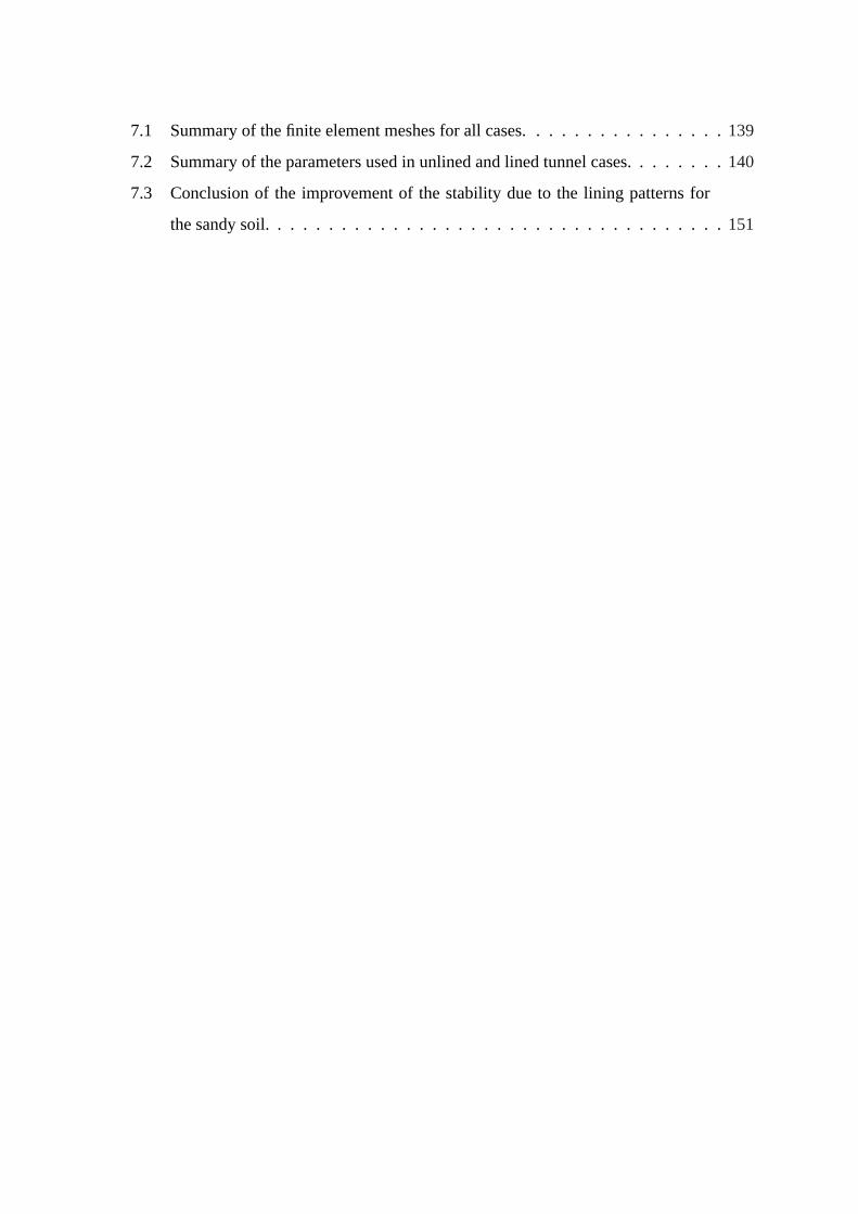
Figure 1.3: Location of the causes of the NATM tunnel collapse(Health and Safety Execu-tive(HSE), 1996)
term ’heading’.
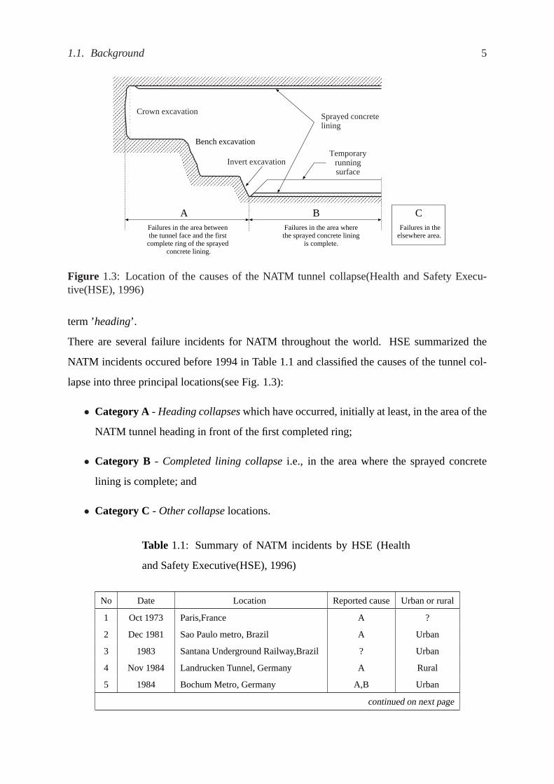
There are several failure incidents for NATM throughout the world. HSE summarized the
NATM incidents occured before 1994 in Table 1.1 and classified the causes of the tunnel col-
lapse into three principal locations(see Fig. 1.3):
• Category A - Heading collapseswhich have occurred, initially at least, in the area of the
NATM tunnel heading in front of the first completed ring;
• Category B - Completed lining collapsei.e., in the area where the sprayed concrete
lining is complete; and
• Category C - Other collapselocations.
Table 1.1: Summary of NATM incidents by HSE (Health
and Safety Executive(HSE), 1996)
No Date Location Reported cause Urban or rural
1 Oct 1973 Paris,France A ?
2 Dec 1981 Sao Paulo metro, Brazil A Urban
3 1983 Santana Underground Railway,Brazil ? Urban
4 Nov 1984 Landrucken Tunnel, Germany A Rural
5 1984 Bochum Metro, Germany A,B Urban
continued on next page

6 Chapter 1. Introduction
Table 1.1 : continued from previous page
6 Jan 1985 Richthof Tunnel, Germany A Rural
7 1985 Bochum Metro, Germany A Urban
8 Aug 1985 Kaiserau Tunnel, Germany A rural
9 Feb 1986 Krieberg Tunnel, Germany A rural
10 Before 1987 Munich Metro, Germany C Urban
11 Before 1987 Munich Metro, Germany A Urban
12 Before 1987 Munich Metro, Germany A Urban
13 Before 1987 Munich Metro, Germany A Urban
14 Before 1987 Munich Metro, Germany A Urban
15 Before 1987 Munich Metro, Germany No collapse Urban
16 Before 1987 Weltkugel Tunnel, Germany A ?
17 1987 Karawanken Tunnel, Austria/Slovenia No collapse Rural
18 Before 1988 Kehrenberg Tunnel, Germany A Rail
19 1988 Michaels Tunnel, Germany A ?
20 Jan 1989 Karawanken Tunnel, Austria/Slovenia A Rural
21 Sep 1991 Kwachon Tunnel, Korea ? Rural
22 Nov 1991 Seoul Metro, Korea A Urban
23 Nov 1991 Seoul Metro, Korea A Urban
24 1992 Funagata Tunnel, Japan C Rural
25 Feb 1992 Seoul Metro, Korea A Urban
26 June 1992 Lambach Tunnel, Austria A ?
27 Jan 1993 Seoul Metro, Korea A Urban
28 Feb 1993 Seoul Metro, Korea A Urban
29 Feb 1993 Seoul Metro, Korea A Urban
30 Feb 1993 Seoul Metro, Korea A Urban
31 Mar 1993 Chungho Tunnel, Taiwan A Rural
32 Nov 1993 Sao Paulo, Brazil A Urban
33 1993 Tuscany, Italy A Rural
34 Apr 1994 Cardvalho Pinto Tunnel, Brazil C ?
35 Jul 1994 Montemor Road Tunnel, Portugal A ?
36 Aug 1994 Montemor Road Tunnel, Portugal A Urban
37 Aug 1994 Galgenberg Tunnel, Austria A Rural
38 Sep 1994 Munich Metro, Germany A Urban
39 Oct 1994 Heathrow Airport, London, UK C Urban
According to Table 1.1, almost the incidents of NATM tunnel collapse occur in the area be-

1.2. Objectives of the research 7
tween the tunnel face and the first complete ring i.e., heading or category A. Therefore, the
evaluation of the stability of tunnel heading is crucial subject to be carried out.
Particularly, the NATM applications in soft ground is extremely difficult because the stand-up
time of soft ground is shorter than that of rock or other stiff ground. In the near surface soft
ground case, the in situ stress will be relatively low, the ground relatively weak and unable
to support redistributed loads. In order to prevent surface buildings suffering damage from
settlement, the shotcrete ring must be closed as early as possible in any soft ground application
of NATM(Muller, 1978) and also the length of the unsupported span (heading) must be left
shorter compared to tunneling in rock. With these reasons, the stability of the tunnel heading
in soft ground(clay) cannot be overlooked and is essential to be considered. In addition, in the
urban area, the shallow tunneling can affect the structures on the ground surface and also the
building load on the surface can affect the tunneling. Therefore, the study on this interaction is
also required.
Furthermore, cause of the collapse of some tunnels, reported in Table 1.1, is due to the high
groundwater pressures acting on the tunnel such as No. 12, 20, 24, 27 and the like. The study
on the effect of the groundwater on the tunnel stability is required.
1.2 Objectives of the research
According to the above-mentioned background, the studies in this dissertation are divided into
two parts; shield tunneling method and New Austrain Tunneling Method. For shield tunneling
method, to solve some problems in other design methods which will be discussed in the subse-
quent chapter, the new structural model for segmental lining is proposed and some applications
of the model is shown. For NATM, the numerical analysis of the tunnel stability in soft ground
is carried out and the effect of groundwater on the tunnel stability will be also studied. The
main objectives of this dissertation are summarized as follows:
Shield tunneling method:
1. To propose the new structural model, calledrigid segment spring model, for the shield
tunnel segment design;
2. To evaluate the application of the model to the actual tunnel (the rectangular tunnel is
considered in this dissertation).

8 Chapter 1. Introduction
New Austrian Tunneling Method:
1. To investigate the stability of tunnel heading in soft clay(purely cohesive soil) consider-
ing the ground as green field;
2. To investigate the effects of the existing super structure on the surface on the tunnel
heading stability;
3. To evaluate the effects of the groundwater on the tunnel stability.
1.3 Scope and organization of the dissertation
Chapter 1 introduces the background of both shield tunneling method and New Austrian Tun-
neling Method, objectives, scope and organization of the dissertation. InChapter 2, for shield
tunneling method, the guideline for design shield tunnel lining is described and some existing
design methods of shield tunnel lining are reviewed. For the NATM, previous researches on the
evaluation of the stability of tunnel face (heading) both in cohesive and in frictional soils are
reviewed. Then, previous studies on the effect of groundwater or seepage force on the tunnel
stability are also described.
In this dissertation, the researches are divided into two parts:Part I : Shield tunneling method;
Part II : New Austrian Tunneling Method (NATM).
Part I deals with the studies relatively to the shield tunneling method and consists of Chapter
3 and Chapter 4.
In Chapter 3, the rigid segment spring model firstly proposed by Tamura et al. (Tamura et al.,
2000) is described. The model is based on the assumption that segments are perfectlyrigid and
connected with three dimensionalpaired-springsat all joints to which the total deformation
of the tunnel is attributed. The formulation of the analysis method using this model for both
circular and rectangular tunnels is described in detail. For more reality on the joint behavior, the
methodology for the consideration of the nonlinear joint spring model is proposed. In general,
the shield tunnel lining is formed by assembling two different segmental rings alternately to
build the staggered joint arrangement. It is apparent that, for long tunnel, the behavior of

1.3. Scope and organization of the dissertation 9
every two adjacent segmental rings which locate far enough away from the boundary ends of
the overall tunnel span, is not much different. The methodology for infinite ring analysis is,
therefore, introduced.
The simulation of the actual shield tunnel segments using the rigid segment spring model is
illustrated inChapter 4. The rectangular ring of the Kyoto Subway Tozai Line Rokujizo-Kita
Construction Section is selected to be simulated. First, the outline of this construction project
is reviewed. In order to fundamentally check the correctness of the analysis model, the prepa-
ration analysis considering the long tunnel as the cantilever beam is carried out. The spring
parameters for this model are unknown hence the parametric study is carried out by simulating
the segmental rings in the full scale segment loading test. The appropriate spring parameters
are obtained by compared the deformation of segmental ring obtained from the simulation
with the observed deformation by test. Finally, the simulation of the in-situ segmental rings
using the appropriate spring parameters is carried out. Both short-term and long-term load-
ing conditions which measured in construction site are considered. The comparison between
the results obtained from the simulation and observed data can indicate that the rigid segment
spring model can be expected to be one effective tool to simulate the shield tunnel segments.
Part II consists of three chapters, namely Chapters 5, 6 and 7. This part illustrates the studies
concerned with the New Austrian Tunneling Method; specifically, stability of tunnel heading
in soft clay and effect of groundwater on the tunnel stability.
Chapter 5 describes the rigid-plastic finite element method (RPFEM) proposed by Tamura
(Tamura et al., 1984; Tamura et al., 1987; Tamura, 1990). The rigid-plastic finite method
is recently considered as the effective tool to determine the critical strength of soil or rock
structures such as dams, tunnels and the foundations for the large structures. Less number
of material parameters is required and solution is independent of the initial condition in this
analysis method. The chapter starts from describing the theoretical basis for plasticity. The
stress-strain rate relations and fundamental equation and boundary conditions for rigid-plastic
analysis are subsequently described. Upper-bound theorem for rigid-plastic analysis is also
explained. Then, the formulation of the RPFEM is described in detail. The methodology to
include the groundwater into the rigid-plastic finite element method is proposed and described.

10 Chapter 1. Introduction
The numerical analysis of the tunnel in soft clay using RPFEM is illustrated inChapter 6. Both
of two and three dimensional analysis for determining the critical state of tunnel are carried out
and the numerical analysis results are taken to compare with the observed data obtained from
the series of centrifugal modeling tests done by Mair(Mair, 1979). The very good agreement
is achieved especially in the two dimensional analysis. In the later section of this chapter, the
study on the influence of the surface load on the stability of plane strain tunnel heading in soft
clay is described.
Chapter 7 studies the effects of the groundwater on the tunnel stability. The RPFEM with
consideration of groundwater which is proposed in Chapter 5 is used to analyze the two di-
mensional cross-section tunnel in various groundwater table. Both of tunnels in clay and sandy
soil are considered. The effect of groundwater on the stability of the unlined tunnel is studied
first. Then, the effect of groundwater on the lined tunnel stability is studied through the various
lining patterns. According to the studies, it is found that the groundwater table affects the un-
lined tunnel stability significantly, especially in sandy soil. For lined tunnel, the tunnel invert
reinforcement is very important if the groundwater table is so high.
Finally, the results presented in each chapter are summarized inChapter 8.

Chapter 2
Literature review
I n this chapter, previous studies on tunneling are reviewed. In the design of the shield tunnel
lining, the outline of the design of shield tunnel lining is described first, followed by exist-
ing design methods for shield tunnel lining. The studies on the evaluation of the tunnel stability
are subsequently reviewed. Finally, the studies on the effect of seepage force or groundwater
on the tunnel stability are reviewed.
2.1 Design of shield tunneling method
2.1.1 Outline of the design of shield tunnel lining
In most cases, the shield tunnel lining consists of the primary lining and the secondary lining,
and is required to maintain a specified internal space by directly supporting the ground. Par-
ticularly, the primary lining is generally formed by assembling the box type or the flat type
factory-manufactured segments which connect to each other by bolt joints in the directions of
tunnel axis and tunnel cross section.
According to Japanese standard for shield tunneling (JSCE, 1996), the basis of the design
of shield tunnel lining is“Design of lining shall based on the confirmation of the safety in
compliance with the purpose of tunnel usage and shall be carried out by the allowable stress
design method on condition that adequate and proper construction works are executed in using
good quality materials”and working group no.2 of International Tunneling Association(ITA)

12 Chapter 2. Literature review
Model to compute member forces
Computation of member forces
Planning of Tunnel Project
AlignmentPlan/ProfileCross Section
Load Condition
Survey/GeologyFunction/Capacityto be given to Tunnel
Specification/Code/Standard to be used
Inner Diameter
Assumption of Lining Condition(thickness, material properties, etc.)
Check the Safety of Lining
Safe and Economical
Approval
Execution of Construction Works
Yes
No
Yes
No
Figure 2.1: Flow chart of shield tunnel lining design
issued a report titledGuidelines for the Design of Shield Tunnel Lining(ITA, 2000). This report
presents a flow chart of shield tunnel lining design as shown in Fig. 2.1 and summarizes the
procedure of the shield tunnel lining design as the following sequence:
1. Adherence to specification, code or standard.The tunnel to constructed should be
designed according to the appropriate specification standard, code which are determined
by the persons in charge of the project.
2. Decision on inner dimension of tunnel.The inner diameter of the tunnel to be designed
should be decided in consideration of the space that is demanded by the functions of the
tunnel.

2.1. Design of shield tunneling method 13
3. Determination of load condition. The following loads should be considered in the de-
sign of shield tunnel lining: earth pressure and water pressure, dead load, surcharge, soil
reaction, internal loads, construction loads and effect of earthquake, etc. The designer
should select the cases critical to the design lining.
4. Determination of lining conditions. The lining conditions that should be designed are
dimension of the lining(thickness), strength of material, arrangement of the reinforce-
ment, etc.
5. Computational of member forces.The designer should compute member forces such
as bending moment, axial force and shear force of the lining, by using appropriate models
and design methods.
6. Safety check.The safety can be checked by considering the computed member forces.
7. Review. If the designed lining is not safe against design loads, the designer should
change the lining conditions and design lining. If the designed lining safe but not eco-
nomical, the designer should change the lining conditions and redesign the lining.
8. Approval of the design. After the designer judges that the designed lining is safe, eco-
nomical and optimally designed, a document of design should be approved by the per-
sons in charge of the project.
According to the above-mentioned procedure of the design of shield tunnel lining, the step 5 is
mainly considered in this dissertation(see the hatched box of flow chart in Fig. 2.1). This step
is the extremely important step of the design of shield tunnel lining. If the appropriate models
or design methods are selected, the computed member forces are close to the actual behavior
of the lining. This leads the obtained lining conditions to be economical and optimal.
2.1.2 Existing segment design methods
There are several design models or design methods of shield tunnel lining so far. The structural
models which are classified by joint evaluation for design of segmental ring are shown in Fig.
2.2. (1) The first model is calledUsual Calculation Method, as shown in Fig. 2.2(a), the
segmental ring is assumed as a ring with uniform bending rigidity without joint is subjected

14 Chapter 2. Literature review
CL
CL
CL
First ring
Second ring
Rotational springs
CL
Hinges
Usual calculation methodModified usual calculation method
Ring with multiple hinged joints
Beam-spring model (I)
(a) (b) (c)
Solid ring with fully bending rigidity and Solid ring with equivalent bending rigidity
Ring with rotational springs and rigid members
CL
CL
First ring
Second ring
Rotational springs
Shear springs
Beam-spring model (II)
(d)
Ring with rotational springs and shear springs
Rigid members
Figure 2.2: Structural models of the segmental ring(Koyama, 2000; JSCE, 1996)
to loading and soil reaction. Since the circumferential joint(segment joint) is assumed to have
the same rigidity as that of the segment, the computed bending moment for the design of joint
is overestimated and bending moment at main section of segment is not calculated correctly
also(Koyama, 2003). Generally, a segmental ring is composed of several segments assembled
by bolts, its deformation tends to be larger than a ring with uniform bending rigidity. This is
because the rigidity of joints is less rigid than a main section of segment. Thus, it is important to
consider the decrease of rigidity at joints for calculating member forces. Moreover because the
staggered joint arrangement is widely used in Japan, the effect of adjacent rings must be also
evaluated. (2) TheModified Usual Calculation Methodhas been introduced to solve the above-
mentioned problem. The decrease of rigidity at segment joints is evaluated by considering the
bending rigidity of segmental ring to be less than that of a ring with uniform bending rigidity by
means of an effective ratio of bending rigidityη. This means, similarly to the Usual Calculation
Method, the bending rigidity of a ring is assumed to be uniform and equal toηEI (η ≤ 1).
In staggered joint arrangement, Some bending moment is transferred to the adjacent ring as
represented byM2 in Fig. 2.3. This redistribution of bending moments are expressed by
introducing a transfer ratio of bending momentζ which is a ratio ofM2/M . M is the bending
moment calculated as a uniform ring ofηEI in rigidity. However, the coefficientη depends on
ground conditions as well as a type of segments, structural character of the segment joint, how
staggered, and structural properties of staggered segmental ring, of which value is determined
by experiences in consideration of joint performance test results and past project records(JSCE,
1996). Moreover, the transfer ratio of bending momentζ and the coefficientη are interrelated
each other. Thus, there is no basis for the determination of these two parameters and it is then

2.1. Design of shield tunneling method 15
Longitudinaldirectionof tunnel
M
M
M= +M1 M2 M1
M2 / 2
M2 / 2
M2 / 2
M2 / 2
B
B/2
B/2M1
M2 / Mη =
= (1−η)M
Figure 2.3: Transferred bending moment to adjacent rings
impossible to calculate actual distribution of the bending moment by using this model.
In the countries where ground condition is good, (3) the Ring with multiple hinged joint cal-
culation method is used. Segment joints are treated as hinges as shown in Fig. 2.2(b). A ring
with multiple hinged joints is an unstable structure by itself but it becomes stable once a ground
supports it. Thus, it is very important to evaluate load distributions acting on the ring and soil
reactions.
For the above reason, In Japan, (4) thebeam-spring model calculation methodis applied nowa-
day. Each segment is considered as a curved beam connected by rotational springs on segment
joints. For the ring joints, for the beam-spring model I, it is assumed that the displacement of
ring beam is equal to that of the adjacent ring beam as shown in Fig. 2.2(c). This means there is
no gap caused by shear stress. shear springs on ring joints. However, the relative displacement
between two adjacent rings also occurs. Therefore, the beam spring model II is also applied.
This relative displacement is expressed by means of the shear spring at ring joints.
According to the above design methods, even though several experiments and analyses have
been carried, but they are only based on 2-dimensional model in cross section of segmental
ring. For 3-dimensional analysis which is required the large scale calculation, the configuration
of boundary condition is very complicated in finite element method. Also, in the beam-spring
model calculation method, even though it can be utilized to analyze the longitudinal direction
of tunnel, it still cannot present the actual three dimensional behavior of tunnel lining.
To solve some problems proposed above, theRigid Segment Spring Modelwhich is first pro-
posed by Tamura et al. (Tamura et al., 2000) is introduced into consideration. This model is
based on the assumption that segments are perfectlyrigid and connected with three dimensional
paired-springsat all joints to which the total deformation of the tunnel is attributed. The model
can simulate the tunnel lining in three dimensional space and does not have many degree of

16 Chapter 2. Literature review
freedom. Also, the offset length between neighboring segments which impossible to determine
by other methods, can be determined by this method. The detail of this model will be described
in the subsequent chapter. Tamura et al.(Tamura et al., 2000) and Hiromatsu(Hiromatsu, 1999)
studied the effect of the staggered joint arrangement by using the rigid segment spring model.
But, the fact that the two adjacent segments cannot overlapped each other was not considered.
In this dissertation, the rigid segment spring model is modified considering the above fact and
improved so that the model can be applied to the actual segmental ring.
2.2 Researches on evaluation of tunnel stability
The safety of the tunnel construction is usually considered into two problems. Firstly, the
stability of tunnel heading (area near the face) is necessary to be evaluated for the safety of
the construction. Secondly, the ground deformation due to the tunneling is also required to be
determined to prevent damage to the existing surface or subsurface structures. Only the first
problem is studied in this dissertation.
Fig. 2.4(a) and 2.4(b) show the layout of tunnel heading problem, where a circular tunnel
of diameterD is constructed with a depth of coverC. The non-supported heading length is
defined byP . The tunnel stability is evaluated by determining the tunnel pressureσT that are
necessary to maintain the stability of the tunnel heading. In addition, the acceleration factor
of weight of soil mass that causes the collapse of tunnel, in accordance with the centrifugal
modeling test concept, can also evaluate the tunnel stability. This section reviews the previous
works on the evaluation of the tunnel stability both in cohesive and frictional ground and some
studies on the effects of groundwater in tunneling are also reviewed.
The stability of tunnel heading in cohesive material(clay) has been studied by several authors
using both experimental and theoretical approaches. Broms and Bennermark (Broms and Ben-
nermark, 1967) conducted the laboratory extrusion tests on soft clay to investigate the stability
of tunnel heading. They indicated that the stability of tunnel heading depends on the term
called stability ratioN which equals to the difference between the total overburden pressure at
the tunnel axis and the tunnel pressure divided by the undrained shear strengthcu as shown in
Eq. (2.1):

2.2. Researches on evaluation of tunnel stability 17
σT
P
D
C
σT
a
a
(b) Section a-a
σS
σS
(a) Transverse section
Figure 2.4: Layout of tunnel heading problem
N =
γ
(C +
D
2
)+ σs − σT
cu
(2.1)
whereσs andγ denote the surface surcharge and the unit weight of soil, respectively. At the
critical state,N andσT are substituted byNC andσTC , respectively. They concluded that
the tunnel face would be stable if the stability ratioN does not exceed6 ∼ 7. Peck(Peck,
1969) collected several case histories on the stability of tunnels in saturated plastic clays and
concluded thatN should not exceed5 ∼ 7 for the stable tunnel face.
A number of centrifugal modeling tests to investigate the stability of tunnel in clay have been
carried out. Mair (Mair, 1979) conducted the centrifugal modeling tests to model both 2D
cross-section tunnels and 3D tunnel headings in clay. Mair also did the numerical analysis us-
ing the Cam-clay model finite element method to analyze some of his experimental results but
the comparison between two approaches does not agree well. Schofield (Schofield, 1980) sum-
marized the experimental data obtained from several three dimensional series of the centrifugal
modeling tests done by Cambridge University into the graph shown in Fig. 2.5.
Takemura et al. (Takemura et al., 1990) and Lee et al. (Lee et al., 1999) carried out the
centrifugal modeling tests to model the 2D cross-section tunnels and also proposed solutions
based on the upper and lower bound theorems to compare with their experimental results. Also,
Davis et al. (Davis et al., 1980) presented a range of solutions based on the upper and lower
bound theorems for unlined plane strain tunnels, circular headings as well as the plane strain
headings. Yu and Rowe(Yu and Rowe, 1999) proposed the plasticity solution using the cavity

18 Chapter 2. Literature review
Figure 2.5: 3D tunnel test data summarized by Schofield(Schofield, 1980)
expansion method for the unlined plane strain tunnel.
In the case of the cohesive-frictional ground, Leca and Dormieux (Leca and Dormieux, 1990)
presented the upper bound solution which represented fairly well the actual behavior of the
tunnel face. Mashimo(Mashimo, 1998) conducted several 2D and 3D tests to investigate the
stability of tunnel face in sandy grounds and concluded that if the dimensionless cohesion
c/(γD) of sandy ground with the angle of frictionφ = 30◦ is approximately not below the
range0.13 ∼ 0.17, the tunnel face is stable.
Murayama (Expressway Technology Center, 1997) proposed the method to evaluate the two
dimensional stability of tunnel heading in sandy ground by using the equilibrium of the moment
acting on the failure soil wedge as shown in Fig. 2.6. This failure line of soil wedge is assumed
to be log-spiral curve and expressed as
r = r0 exp(θ tan φ). (2.2)
The resultant forceP to maintain the tunnel face can be determined by using the equilibrium
equation of the moment, caused by the 5 forces acting on soil wedge, around the centerO of
the spiral curve. The resultant forceP is written as
P =1
lp
{W × lw + q ×B
(la +
B
2
)− c
2 tan φ
(r2c − r2
0
)}(2.3)
in which the Terzaghi’s loosening earth pressureq acting on the widthαB of the top of wedge

2.2. Researches on evaluation of tunnel stability 19
θ
o
α0
P
R
Bl a
αB
q
a b
c
W
l w
F φ
r0
rc
r
Ove
rbur
den
Hei
ght o
f he
adin
g
l p
Figure 2.6: Force equilibrium on soil wedge in method for evaluating tunnel face stabilityproposed by Murayama
is
q =αB (γ − 2c/αB)
2K tan φ
[1− exp(−2KC/αB) tan φ
](2.4)
or, if the overburdenC is much larger thanB, approximatelyC > 1.5B, Eq. (2.4) can be
reduced to
q =αB (γ − 2c/αB)
2K tan φ(2.5)
and some notations are introduced asγ : unit weight of soil
φ : angle of internal friction
c : cohesion of soil
K : the ratio of the horizontal earth pressure to vertical earth pressure
(K = 1 ∼ 1.5)
r0, rc : the radius of the log-spiral curve measured from pointb andc, respectively
α : coefficient to indicate the loosening width (according to experiments,α ≈ 1.8).Toki and Tamura et al.(Toki et al., 1994) also proposed the simplified method to evaluate the
2D tunnel face stability. They assumed the failure wedge as the triangular wedge and its linear
failure line connects pointb and pointc as shown in Fig. 2.7. The resultant forceP to maintain
the tunnel face is calculated by equating all forces acting on the wedge both in horizontal and

20 Chapter 2. Literature review
PD
D tanβ
a b
c
W
φN 2
β
N 1
T1
T2
q
=q D tanβ
Figure 2.7: Force equilibrium on soil wedge in method for evaluating tunnel face stabilityproposed by Tamura et al.
vertical directions. The forceP is expressed as
P =
{1
2γD tan β + q(tan β − tan φ)− 3c
}D tan β (2.6)
whereβ = 45◦ − φ/2 and the Terzaghi’s loosening earth pressureq is the same as that of Eq.
(2.4) butαB is substituted byD tan β.
According to both of Murayama’s method and Tamura’s method, the tunnel can be stable by
itself if the resultant forceP is not positive.
For cohesionless soil, Atkinson and Potts (Atkinson and Potts, 1977) investigated theoretically
and experimentally the stability of a circular tunnel in a cohesive soil. They conducted small-
scale model tests and used the centrifuge of the Cambridge University and also derived some
solutions, based on the upper and lower bound theorems, to predict the tunnel pressure at
collapse.
The finite element method is also used to investigate stability of tunnel heading by many au-
thors. Eisenstein and Samarasekara (Eisenstein and Samarasekera, 1992) examined the stabil-
ity of tunnels in clay using a combination of the finite element method and the limit equilibrium
theory. Sloan et al. and Augarde et al. (Sloan and Assadi, 1994; Augarde et al., 2003) pre-
sented the finite element limit analysis method considering the upper bound analysis and the
lower bound analysis independently by using nonlinear programming. However, these works
were based on merely the two-dimensional analysis. The rigid-plastic finite element method

2.3. Effects of groundwater on the tunnel stability 21
(RPFEM) based on upper bound theorem, developed by Tamura (Tamura et al., 1984; Tamura
et al., 1987; Tamura, 1990), is one of the effective approaches for evaluation of the bearing
capacity and the stability of slopes and tunnel faces. Tamura et al. (Tamura et al., 1999) firstly
presented the use of RPFEM to simulate the tunnel face stability problems, mainly in sandy
ground. Konishi (Konishi, 2000) studied the stability of tunnel face in the ground of alternate
layers (sandy and cohesive soils) by conducting the 3D experimental tests and comparing the
test results with RPFEM both in two and three dimensional analysis. He found that RPFEM
can simulate the stability of tunnel face in the ground of alternate layers effectively.
2.3 Effects of groundwater on the tunnel stability
The studies on the evaluation of the stability of tunnel face are done by several authors in the
last thirty years. But there are very few studies that consider the effects of groundwater on
the stability of the tunnel face. Pollet et al.(Pellet et al., 1993) carried out a three-dimensional
finite element analysis of groundwater flow and concluded that the head losses are concentrated
in the close vicinity of the tunnel face i.e., seepage forces acting on the tunnel face exists.
They also conducted several three-dimensional tests to investigate the mechanical behavior
and stability of the microtunnel face in soft ground. The observed supporting pressures at
tunnel face were compared with the supporting pressures calculated from the elasto-plastic
finite element method in plane strain condition. Buhan et al. (Buhan et al., 1999) determined
the tunnel pressure that stabilize the tunnel face by comparing the equilibrium of the conical
volume, suggested by Leca and Dormieux(Leca and Dormieux, 1990), of soil subjected to the
combined effect of gravity and seepage forces and the Mohr-Coulomb yield criterion. The
seepage forces were determined by the 3D seepage finite element analysis.
Lee and Nam (Lee and Nam, 2001) calculated the minimum supporting pressure at the tunnel
face by summing up the upper bound solution proposed by Leca and Dormieux (Leca and
Dormieux, 1990), based on effective stress analysis, and seepage forces acting on the tunnel
face, calculated from the 3D seepage finite element analysis. Also, Lee et al.(Lee et al., 2003)
verified the calculated results of the numerical analysis by comparing them with the observed
values of the model tests. They found the very good agreement between the two approaches.
Droniuc et al.(Droniuc et al., 2004) studied the effect of groundwater on the stability of tunnel

22 Chapter 2. Literature review
face in cohesive-frictional soil by using the regularized kinematical approach of limit analysis,
developed at LCPC(Laboratoire Central des Ponts et Chaussees), formulated by finite element
method. The results calculated from the numerical analysis were agreed well with those ob-
tained from the method proposed by Lee and Nam(Lee and Nam, 2001).
Konishi and Tamura (Konishi and Tamura, 2002; Konishi et al., 2003) proposed the method
to include the groundwater into the rigid-plastic finite element method and carried out some
fundamental studies on the effect of the groundwater on the simple geotechnical problems and
simple tunnel problems. But, this method can analyze only the problem with non-dilatant
condition in soil(non-associated flow rule).
In this dissertation, the new method which can analyze both associated and non-associated
flow rules, to include the groundwater into the RPFEM is proposed and then some fundamental
studies of the effect of groundwater on the tunnel stability will be carried out.

Part I
Shield tunneling method
23


Chapter 3
Rigid segment spring model
3.1 Introduction
G enerally, the shield tunnel lining is composed of the primary lining and secondary lin-
ing. Particularly, the primary lining is often formed by assembling the box type or
the flat type factory-manufactured segments which connect to each other by bolt joints in the
directions of tunnel axis and tunnel cross section. There are several methods to design the
shield tunnel segment such as the usual calculation method, the beam-spring model calcula-
tion method and the finite element method. In this chapter, new alternative design method, so
calledrigid segment spring model, is proposed and described in detail. Not only the conven-
tional circular ring but also the rectangular ring of the Kyoto Subway Tozai line(Rokujizo-Kita
Construction Section Project), can be analyzed by this model. Therefore, the methodology to
analyze the circular rings by this model is explained as well as the rectangular rings.
In this chapter, the description of the model is explained first. Then, some main governing
equations including the matrix formulation of the model are described. Morever, for more
reality in the application of the model to the actual rings, the algorithm for considering the
nonlinear joint-spring model is described.
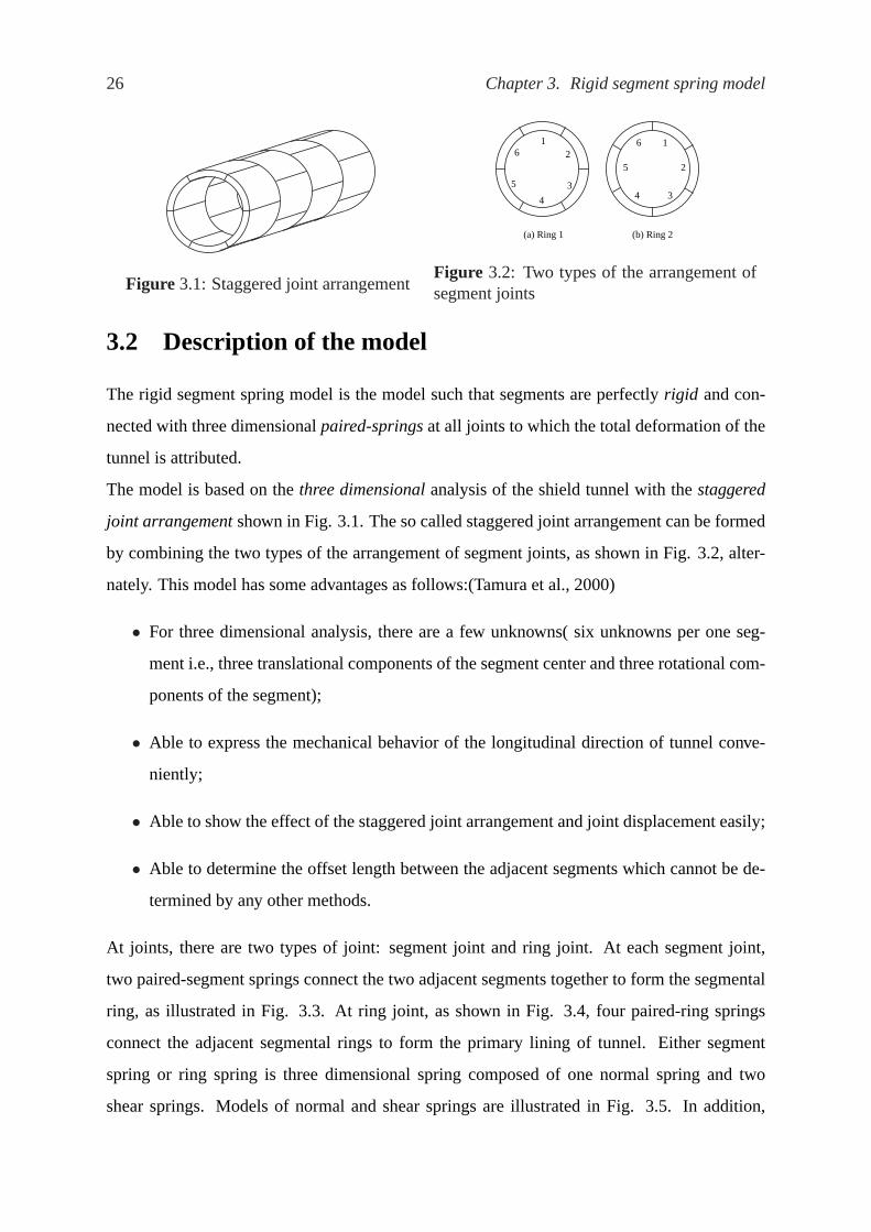
26 Chapter 3. Rigid segment spring model
Figure 3.1: Staggered joint arrangement
(a) Ring 1 (b) Ring 2
12
3
4
5
61
2
34
5
6
Figure 3.2: Two types of the arrangement ofsegment joints
3.2 Description of the model
The rigid segment spring model is the model such that segments are perfectlyrigid and con-
nected with three dimensionalpaired-springsat all joints to which the total deformation of the
tunnel is attributed.
The model is based on thethree dimensionalanalysis of the shield tunnel with thestaggered
joint arrangementshown in Fig. 3.1. The so called staggered joint arrangement can be formed
by combining the two types of the arrangement of segment joints, as shown in Fig. 3.2, alter-
nately. This model has some advantages as follows:(Tamura et al., 2000)
• For three dimensional analysis, there are a few unknowns( six unknowns per one seg-
ment i.e., three translational components of the segment center and three rotational com-
ponents of the segment);
• Able to express the mechanical behavior of the longitudinal direction of tunnel conve-
niently;
• Able to show the effect of the staggered joint arrangement and joint displacement easily;
• Able to determine the offset length between the adjacent segments which cannot be de-
termined by any other methods.
At joints, there are two types of joint: segment joint and ring joint. At each segment joint,
two paired-segment springs connect the two adjacent segments together to form the segmental
ring, as illustrated in Fig. 3.3. At ring joint, as shown in Fig. 3.4, four paired-ring springs
connect the adjacent segmental rings to form the primary lining of tunnel. Either segment
spring or ring spring is three dimensional spring composed of one normal spring and two
shear springs. Models of normal and shear springs are illustrated in Fig. 3.5. In addition,

3.3. Coordinate systems 27
Two adjacent segments
Figure 3.3: Description of segment springs
Two adjacent rings
Figure 3.4: Description of ring springs
(a) Normal spring (b) Shear spring
Figure 3.5: Normal and shear spring models
for each segment, three dimensional ground reaction springs connect six external nodes to the
surrounding ground and six internal nodes to some supports inside the tunnel as shown in Fig.
3.6(a). The three components of each three dimensional ground reaction spring are all normal
spring as illustrated in Fig. 3.6(b).
External nodes
Internal nodes
3
1
2
k1
k2
k3
(a) (b)
Figure 3.6: Description of ground reaction springs:(a) Positions of springs, (b) three directionsof each spring

28 Chapter 3. Rigid segment spring model
X
Y
Z
side view
top view
l
l
l
ZZ
X Y
(a) Local coordinate of circular segment (b) Global coordinate of circular tunnel
Xl
1 2 3Ring number
. . .
Figure 3.7: Coordinate systems of circular tunnel
3.3 Coordinate systems
3.3.1 Local and global coordinates
There are two coordinate systems in this analysis: local coordinate system and global coor-
dinate system. For coordinate systems of simple circular ring analysis, all of segments have
totally the same size thus, local coordinate system of each segment is also the same as illustrate
in Fig. 3.7(a) and global coordinate system is illustrated in Fig. 3.7(b). Segmentj of ring i is
defined as segment(i, j). The segment number of each ring is defined increasingly clockwise
as shown in Fig. 3.2. Ring number is defined increasingly in the positive direction of tunnel
axis (globalY axis) as shown in Fig. 3.7(b). If total number of rings is more than two, the
arrangement of segment numbers in each ring is given by Fig. 3.8.
For the rectangular ring analysis, dimension of each segment is different, thus it is necessary
to define specifically the local coordinate systems. The local coordinate systems of segments
in ring 1 and ring 2 are illustrated in Figs. 3.9(a) and 3.9(b), respectively. Global coordinate
system of rectangular ring case is shown in Fig. 3.10. It should be noted that local coordinate
system of each segment is defined on the concept thatZ-axis of segment(i, j) is parallel to
edge of segment of neighboring rings as shown in Fig. 3.11. As the same as in the circular ring
analysis, if total number of rings is more than two, the setting of segment numbers surrounding
segment no.(i, j) used in programming is illustrated in Fig. 3.8.

3.3. Coordinate systems 29
i , j
i+1 , ji+1 , j-1
i-1, ji -1, j+1
i , j+1i , j-1 Ring i+1
Ring i
Ring i-1
Figure 3.8: Arrangement of numbers of segments in analysis if total number of rings> 2
3.3.2 Coordinate transformation
Since this analysis is carried out by considering both of global coordinate system and local
coordinate system of each segment, the transformation between these coordinate systems is
described here.
Relationship between Local coordinate systems
Firstly, consider the relationship between local coordinates of segment(i, j) and its neigh-
boring segments. As shown in Fig. 3.12, theX-axis andZ-axis of segments(i − 1, j) and
(i + 1, j − 1) can be obtained by rotatingX andZ axis of segment(i, j) counterclockwise
aroundY -axis through the angleθ(i−1,j)(i,j) andθ
(i+1,j−1)(i,j) , respectively. On the other hand,X-axis
andZ-axis of segments(i − 1, j + 1) and (i + 1, j) can be obtained by rotatingX andZ
clockwise through the angleθ(i−1,j+1)(i,j) andθ
(i+1,j)(i,j) , respectively.
Transformation matrix for two vectors
Firstly, rotation of coordinates in this transformation is supposed as:
Consider two sets of rectangular Cartesian frames of referenceo− x1x3 and newo′ − x′1x′3 on
a plane. If origin remains fixed, and the new axeso′ − x′1x′3 are obtained by rotatingox1 and
ox3, aroundox2 axis, through an angleθ, as shown in Fig 3.13. If the rotation is done in the
clockwise direction, and pointP has coordinates(x1, x1, x3) and(x′1, x′2, x
′3) with respect to

30 Chapter 3. Rigid segment spring model
iNote : segment no. inode no. 22x-axis through that point
4
5
6
1
37
237
2
1
2
5
2
5
2
5
x3
x4 z
4z5
x5
z6
x6
z7
x7
z1 x
1
z2
x2
z3
y7
y1
y2
x1
x7
x2
5
4
3
1
6
76 2
2
1
2
5
2
5
2
5
7
z7
x7
z1
x1 x
2
z2
z3
x3
z4
x4
z5
x5
z6
x6
y7
y1
y2
x7
x1
x2
(a) Ring 1 (b) Ring 2
Figure 3.9: Global coordinates of rectangular tunnel
Z
X
Z
Y
Figure 3.10: Global coordinates of rectangular tunnel

3.3. Coordinate systems 31
segment (i, j)
Z
X
(i , j)
(i , j)
edge of segment of neighboring ring
segment (i -1 , j+1) or (i + 1 , j )
segment (i - 1 , j) or (i + 1 , j -1)
segment (i , j) tunn
el a
xis Top view
Figure 3.11: Concept of local coordinatesystem setting
(i - 1 , j) (i - 1 , j+1)
(i-1 , j+1)
(i , j) θ
(i+1, j-1)or
(i+1, j)or
(i+1 , j)
(i , j) θ
(i-1 , j)
(i , j) θ
(i+1, j-1)
(i , j) θor or
(i , j)
Figure 3.12: Relationship between localcoordinates of segment(i, j) and its neigh-boring segments in adjacent rings
the old and new frames of reference, respectively, then
x′1
x′2
x′3
=
cos θ 0 − sin θ
0 1 0
sin θ 0 cos θ
x1
x2
x3
(3.1)
or, in the another form:
x′ = Rx. (3.2)
It can be seen that we can transformx to x′ by using a orthogonal tensorR. Similarly, dis-
placement vector and force vector can be transformed to the new one by usingR as follows:
u′ = Ru and, (3.3)
f ′ = Rf . (3.4)
Inversely, if the rotation is done in the counterclockwise direction, we can get
x′1
x′2
x′3
=
cos θ 0 sin θ
0 1 0
− sin θ 0 cos θ
x1
x2
x3
(3.5)

32 Chapter 3. Rigid segment spring model
θ
θ
θ
θ
(a) Counterclockwise rotation (b) Clockwise rotation
O, O’ O, O’
x3
x’1
x1
x’3
x3 x’
3
x1
x’1
Figure 3.13: Rotation of coordinate axis: counterclockwise and clockwise direction
or, in the another form:
x′ = R−1x. (3.6)
SinceR is orthogonal tensor which has property that
R−1 = RT , (3.7)
RT can be used instead ofR−1. In this sense,R andRT can be used to transform between
segment coordinates. For example, as seen in Fig 3.12, in order to transform the local coordi-
nates of segment(i − 1, j) to the local coordinates of segment(i, j) the orthogonal tensorR1
can be used as a transformation tensor as shown symbolically as:
(i− 1, j)R1−→ (i, j) (3.8)
where,R1 is defined as
R1 =
cos[θ
(i−1,j)(i,j)
]0 sin
[θ
(i−1,j)(i,j)
]
0 1 0
− sin[θ
(i−1,j)(i,j)
]0 cos
[θ
(i−1,j)(i,j)
]
. (3.9)
3.3.3 Matrix of spring constants
As mentioned previously, all of springs are 3-dimensional springs and then directions of spring
constants are supposed ask1, k2 andk3 with respect to each direction, respectively. From

3.3. Coordinate systems 33
3
1
3’3’’
1’
1’’
θ1
o
θ2
Figure 3.14: Set of three frames of reference
Hooke’s laws:
fi = kiui (3.10)
where,fi is force in directioni andui is displacement of spring in directioni.
Therefore, the relation between spring force vector and spring displacement can be expressed
as follows:
f = Ku (3.11)
or, by showing theirs components;
f1
f2
f3
=
k1 0 0
0 k2 0
0 0 k3
u1
u2
u3
. (3.12)
According to Eq. (3.11),K is calledspring constant matrix.
Now, suppose that force vectorf is transformed tof ′ of new frame of reference by rotating in
clockwise direction through an angleθ1 and; also, displacement vectoru is transformed tou′′
of new frame of reference by rotating in clockwise direction through an angleθ2, as illustrated
in Fig 3.14. Thus, from Eqs. (??) and (3.4) by using different matrixR, we can obtain
f ′ = R1f or f = RT1 f ′ (3.13)
u′′ = R2u or u = RT2 u′′. (3.14)

34 Chapter 3. Rigid segment spring model
112
611
5
10
4
3
7 8
2
9
Figure 3.15: Numbers of nodes connected with ground reaction springs in circular ring case
1320
1916
15
17
1418
Figure 3.16: Numbers of nodes connectedwith segment springs in circular ring case
2136
3530
29
27
2228
26
2523
24
34
3331
32
Figure 3.17: Numbers of nodes connectedwith ring springs in circular ring case
After the transformation, suppose that we will get the following equation:
f ′ = Kfu′′. (3.15)
Combine Eq. (3.11) and Eq. (3.14) then substitute it into Eq. (3.13); and compare the result to
Eq. (3.15), then
Kf = R1KRT2 (3.16)
is obtained.
3.4 Spring position setting
The position of each spring will be explained in this section. Each type of set of springs
connects to different set of node numbers as described below.

3.4. Spring position setting 35
1
4
32
5 6
121110
987
13
14
17
18
15 19
2016 21
22 2624
23 25
3331
30
29
3432
35
3627
28
4 15
21
22
23
24
25
26
27
28
29
30
3132
3334
35
3613
14
16 17
18
19
201 2 3
5 6
7 8 9
10 11 12
1
2
3
4
5
6
7
8
9
10
11
12
13
14
15
16
1718
1920
29
21
22
2324
2526
2728
30
3132
3334
3536
1
23
4
5 6
7
89
10
11 12
13 14
1516
17
18
19
20
21 22
23
24
25
26
27
28
29 30
31
32
33
34
35
36
123
456
101112
78
9
13
14 15
16
17
1819
20
21
22
23
24
25
26
27
2829
30
31
32
33
34
35
36
1
3, 6
5
4, 7
ground reaction ring jointsegment joint
2
seg No.
(Key segment)
Figure 3.18: Numbers of nodes connected with each type of springs in rectangular ring 1

36 Chapter 3. Rigid segment spring model
1
ground reaction ring jointsegment joint
4
12
6
11
5
103
9
2
87
1
15
13
14
19
2017
18
16
29
21
22
30
24
23 25
26 28
27 36
353331
32 34
2 , 5 14
13
15
16
17
1920
21 23
24
25
26
2728
29
30
31
32
33
34
3536
4
1
78
2
11
5
612
3
10
22
4
21
22
23
24
25
26
27
2829
30
31
32
33
34
35
36
13
1415
16
17
1819
20
123
456
101112
78
9
7 4
1 23
5 6
7 8 9
1011 12
15
13
14
16 17
18
19
2021
22
23
24
25
26
27
28
29
30
3132
33
3435
36
3, 6
1
2
3
4
5
6
7
8
9
10
11
12
13 14
1516
17
18
19
20
35
29
21 22
23 24
25 26
27
28
30
31 32
33 34
36
189
seg No.
(Key segment)
Figure 3.19: Numbers of nodes connected with each type of springs in rectangular ring 2

3.4. Spring position setting 37
3.4.1 Ground reaction spring
Ground reaction springs connect each segment to surrounding support at the nodes no.1 to no.
12, as illustrated in Fig. 3.15 for circular ring analysis or Fig. 3.18 and 3.19 for rectangular
ring analysis. At each connecting node, ground reaction spring has 3 directions;k1, k2 andk3,
as shown in Fig. 3.6(b).
Ground reaction spring constant matrices of node no.k = 1 ∼ 12 of segment(i, j) are denoted
by iK1j ∼ iK
12j .
3.4.2 Segment joint spring
Segment springs are placed at the nodes no.13 to no. 20, as illustrated in Fig. 3.16 for circular
ring analysis or Figs. 3.18 and 3.19 for rectangular ring analysis. At each connecting node,
segment spring has 3 directions: one normal spring constant; two shear spring constants.
Segment spring constant matrices of nodek = 17 ∼ 20 of segment(i, j) are denoted byiK13j
∼ iK16j . These four segment springs connect nodek = 17 ∼ 20 of segment(i, j) to node no.
k = 13 ∼ 16 of segment(i, j + 1), individually.
3.4.3 Ring joint spring
Ring springs are placed at the nodes no.21 to no. 36, as illustrated in Fig. 3.17 for circular
ring analysis or Figs. 3.18 and 3.19 for rectangular ring analysis. At each connecting node,
similar to segment spring, ring spring has 3 directions: one normal spring constant and two
shear spring constants.
Segment spring constant matrices of nodek = 29 ∼ 36 of segment(i, j) are denoted by
iK17j ∼ iK
24j . These eight ring springs are divided into 2 parts equally; first four ring springs
connect nodek = 29 ∼ 32 of segment(i, j) to nodek = 25 ∼ 28 of segment(i+1, j−1) and
the another four ring springs connect nodek = 33 ∼ 36 of segment(i, j) to nodek = 21 ∼ 24
of segment(i + 1, j).

38 Chapter 3. Rigid segment spring model
3.5 Reaction force of spring
The equilibrium equation of each segment is used corresponding in local coordinate system of
segment. In any segment(i, j), the reaction forces of springs at all nodes are brought into the
equilibrium equation and, finally, the unknown vectorx will be obtained by using Eq. (A.38).
Here, some symbols used in this section are explained. Firstly, the definitions of subscripts and
superscripts of symbol(i,j)l Akm is shown as follows:
• Left superscript(i, j) means quantityA is considered relatively to the local coordinate
of segment(i, j);
• Left subscriptl means quantityA is the quantity of ring no.l;
• Right subscriptm means quantityA is the quantity of segment no.m;
• Right superscriptk means quantityA is the quantity of node no.k.
Conclusively, (i,j)l Ak
m means the quantityA of node no.k of segment(l, m) relative to the
local coordinates of segment(i, j). Next, R(m,n)(i,j) and θ
(m,n)(i,j) are the orthogonal tensor and
the difference of angles between local coordinates of segment(i, j) and local coordinates of
segment(m,n), respectively.R(m,n)(i,j) can be represented corresponding toθ
(m,n)(i,j) as
R(m,n)(i,j) =
cos[θ
(m,n)(i,j)
]0 − sin
[θ
(m,n)(i,j)
]
0 1 0
sin[θ
(m,n)(i,j)
]0 cos
[θ
(m,n)(i,j)
]
. (3.17)
3.5.1 Ground reaction spring
k = 1, 4, 7, 10
According to Figs. 3.15 and 3.8, 3 directions of ground reaction spring are parallel to 3 direc-
tions of(i + 1, j − 1) coordinate axes. Thus, by referring to coordinate system(i + 1, j − 1),
Eq. (3.11) can be written as
(i+1,j−1)i fk
j = − iKkj
(i+1,j−1)i uk
j . (3.18)

3.5. Reaction force of spring 39
Next, the transformation(i + 1, j − 1)R(i,j)
(i+1,j−1)−−−−−−→ (i, j) will be carried out. SupposeiQkj be
tensorQ of Eq. (A.38), Eq. (A.38) can be written in this form:
(i,j)i uk
j = iQkj ixj. (3.19)
By using the transformation(i + 1, j − 1)R(i,j)
(i+1,j−1)−−−−−−→ (i, j) and Eq. (3.18),
(i,j)i fk
j = −(R
(i,j)(i+1,j−1)
)iK
kj
(R
(i,j)(i+1,j−1)
)TiQ
kj ixj
= − iDkj ixj
(3.20)
where,
iDkj = −(
R(i,j)(i+1,j−1)
)iK
kj
(R
(i,j)(i+1,j−1)
)TiQ
kj (3.21)
is obtained.
k = 2, 5, 8, 11
Three directions of ground reaction spring are parallel to 3 directions of(i, j) coordinate axes.
Thus, by referring to coordinate system(i, j), Eq. (3.11) can be written as
(i,j)i fk
j = − iKkj
(i,j)i uk
j . (3.22)
SupposeiQkj be tensorQ of Eq. (A.38), Eq. (A.38) can be written in the following form:
(i,j)i uk
j = iQkj ixj. (3.23)
Then, Eq. (3.22) can be rewritten as
(i,j)i fk
j = − iKkj iQ
kj ixj
= − iDkj ixj
(3.24)
where,
iDkj = iK
kj iQ
kj . (3.25)
k = 3, 6, 9, 12

40 Chapter 3. Rigid segment spring model
Three directions of ground reaction spring are parallel to 3 directions of(i + 1, j) coordinate
axes. Thus, by referring to coordinate system(i + 1, j), Eq. (3.11) can be written as
(i+1,j)i fk
j = − iKkj
(i+1,j)i uk
j . (3.26)
Next, the transformation(i + 1, j)
(R(i,j)
(i+1,j)
)T
−−−−−−−→ (i, j) will be carried out. SupposeiQkj be
tensorQ of Eq. (A.38), Eq. (A.38) can be written in the form:
(i,j)i uk
j = iQkj ixj. (3.27)
By using the transformation(i + 1, j)
(R(i,j)
(i+1,j)
)T
−−−−−−−→ (i, j) and Eq. (3.26), the following equation
is obtained.
(i,j)i fk
j = −(R
(i,j)(i+1,j)
)TiK
kj
(R
(i,j)(i+1,j)
)iQ
kj ixj
= − iDkj ixj
(3.28)
where,
iDkj = −(
R(i,j)(i+1,j)
)TiK
kj
(R
(i,j)(i+1,j)
)iQ
kj . (3.29)
3.5.2 Segment spring
In one segment, there are two edges which connected by segment springs to previous and next
segments, respectively. Thus following explanation will be divided into two cases:
Connecting to the previous segment (k = 13, 14, 15, 16)
According to Figs. 3.16 and 3.8, node(i, j, 13) ∼ (i, j, 16) are connected by springs no.
(i, j − 1, 13) ∼ (i, j − 1, 16) to node(i, j − 1, 17) ∼ (i, j − 1, 20). 3 directions of segment
spring are parallel to 3 directions of(i + 1, j − 1) coordinate axes. Thus, by respecting to
coordinate system(i + 1, j − 1), Eq. (3.11) can be written as
(i+1,j−1)i fk
j = iKkj−1
[(i+1,j−1)i uk+4
j−1 − (i+1,j−1)i uk
j
]. (3.30)

3.5. Reaction force of spring 41
For (i+1,j−1)i fk
j and (i+1,j−1)i uk
j , the transformation(i + 1, j − 1)R(i,j)
(i+1,j−1)−−−−−−→ (i, j) is carried
out and, for (i+1,j−1)i uk+4
j−1 , the transformation(i + 1, j − 1)
(R(i,j−1)
(i+1,j−1)
)T
−−−−−−−−→ (i, j − 1) is carried
out. Then, Eq. (3.30) can be expressed in following form:
(i,j)i fk
j =(R
(i,j)(i+1,j−1)
)iK
kj−1
[(R
(i,j−1)(i+1,j−1)
) (i,j−1)i uk+4
j−1 −(R
(i,j)(i+1,j−1)
)T (i,j)i uk
j
]. (3.31)
Next, Eq. (A.38) can be written in the following forms:
(i,j−1)i uk+4
j−1 = iQk+4j−1 ixj−1 (3.32)
(i,j)i uk
j = iQkj ixj. (3.33)
Substitute Eqs. (3.32) and (3.33) into Eq. (3.31), obtain
(i,j)i fk
j =(R
(i,j)(i+1,j−1)
)iK
kj−1
(R
(i,j−1)(i+1,j−1)
)iQ
k+4j−1 ixj−1
− (R
(i,j)(i+1,j−1)
)iK
kj−1
(R
(i,j)(i+1,j−1)
)TiQ
kj ixj
= iCkj ixj−1 − iD
kj ixj
(3.34)
where,
iCkj =
(R
(i,j)(i+1,j−1)
)iK
kj−1
(R
(i,j−1)(i+1,j−1)
)iQ
k+4j−1 (3.35)
iDkj =
(R
(i,j)(i+1,j−1)
)iK
kj−1
(R
(i,j)(i+1,j−1)
)TiQ
kj . (3.36)
Connecting to the next segment (k = 17, 18, 19, 20)
According to Figs. 3.16 and 3.8, node(i, j, 17) ∼ (i, j, 20) are connected by springs no.
(i, j, 13) ∼ (i, j, 16) to node(i, j + 1, 13) ∼ (i, j + 1, 16). 3 directions of segment spring are
parallel to 3 directions of(i + 1, j) coordinate axes. Thus, by referring to coordinate system
(i + 1, j), Eq. (3.11) can be written as
(i+1,j)i fk
j = iKk−4j
[(i+1,j)i uk−4
j+1 − (i+1,j)i uk
j
]. (3.37)
For (i+1,j)i fk
j and (i+1,j)i uk
j , the transformation(i + 1, j)
(R(i,j)
(i+1,j)
)T
−−−−−−−→ (i, j) is carried out and,

42 Chapter 3. Rigid segment spring model
for (i+1,j)i uk−4
j+1 , the transformation(i + 1, j)R(i,j+1)
(i+1,j)−−−−→ (i, j + 1) is carried out. Then, Eq. (3.37)
can be expressed in following form:
(i,j)i fk
j =(R
(i,j)(i+1,j)
)TiK
k−4j
[(R
(i,j+1)(i+1,j)
)T (i,j+1)i uk−4
j+1 −(R
(i,j)(i+1,j)
) (i,j)i uk
j
]. (3.38)
Next, Eq. (A.38) can be written in the following forms:
(i,j+1)i uk−4
j+1 = iQk−4j+1 ixj+1 (3.39)
(i,j)i uk
j = iQkj ixj (3.40)
Substitute Eqs. (3.39)) and (3.40) into Eq. (3.38), then we obtain
(i,j)i fk
j = −(R
(i,j)(i+1,j)
)TiK
k−4j
(R
(i,j)(i+1,j)
)TiQ
kj ixj
+(R
(i,j)(i+1,j)
)TiK
k−4j
(R
(i,j+1)(i+1,j)
)iQ
k−4j+1 ixj+1
= − iDkj ixj + iE
kj ixj+1
(3.41)
where,
iDkj =
(R
(i,j)(i+1,j)
)TiK
k−4j
(R
(i,j)(i+1,j)
)TiQ
kj (3.42)
iEkj =
(R
(i,j)(i+1,j)
)TiK
k−4j
(R
(i,j+1)(i+1,j)
)iQ
k−4j+1 . (3.43)
3.5.3 Ring spring
At the ring spring connections, we can divided them into 4 parts:k = 21 ∼ 24; k = 25 ∼ 28;
k = 29 ∼ 32 andk = 33 ∼ 36 (see Fig. 3.17). Each part will be discussed as follows:
k = 21, 22, 23, 24
According to Figs. 3.17 and 3.8, node(i, j, 21) ∼ (i, j, 24) are connected by springs no.
(i − 1, j, 21) ∼ (i − 1, j, 24) to node(i − 1, j, 33) ∼ (i − 1, j, 36). By the assumption that
isotropic shear spring, spring force acting at node(i, j, k), with respect to coordinate system

3.5. Reaction force of spring 43
(i, j), can be expressed as
(i,j)i fk
j = i−1Kkj
[(i,j)i−1u
k+12j − (i,j)
i ukj
]. (3.44)
For (i,j)i−1u
k+12j , the transformation(i− 1, j)
R(i,j)(i−1,j)−−−−→ (i, j) is carried out. Then, Eq. (3.44) can
be expressed in following form:
(i,j)i fk
j = i−1Kkj
[(R
(i,j)(i−1,j)
) (i−1,j)i−1 uk+12
j − (i,j)i uk
j
]. (3.45)
Next, Eq. (A.38) can be written in the following forms:
(i−1,j)i−1 uk+12
j = i−1Qk+12j i−1xj (3.46)
(i,j)i uk
j = iQkj ixj. (3.47)
Substitute Eqs. (3.46)) and (3.47) into Eq. (3.45), then we obtain
(i,j)i fk
j = i−1Kkj
(R
(i,j)(i−1,j)
)i−1Q
k+12j i−1xj − i−1K
kj iQ
kj ixj
= iAkj i−1xj − iD
kj ixj
(3.48)
where,
iAkj = i−1K
kj
(R
(i,j)(i−1,j)
)i−1Q
k+12j (3.49)
iDkj = i−1K
kj iQ
kj . (3.50)
k = 25, 26, 27, 28
According to Figs. 3.17 and 3.8, node(i, j, 25) ∼ (i, j, 28) are connected by springs no.
(i − 1, j + 1, 17) ∼ (i − 1, j + 1, 20) to node(i − 1, j + 1, 29) ∼ (i − 1, j + 1, 32). By
the assumption that isotropic shear spring, spring force acting at node(i, j, k), with respect to
coordinate system(i, j), can be expressed as
(i,j)i fk
j = i−1Kk−8j+1
[(i,j)i−1 uk+4
j+1 − (i,j)i uk
j
]. (3.51)

44 Chapter 3. Rigid segment spring model
For (i,j)i−1u
k+4j+1 , the transformation(i− 1, j + 1)
(R(i,j)
(i−1,j+1)
)T
−−−−−−−−→ (i, j) is carried out. Then, Eq.
(3.51) can be expressed in following form:
(i,j)i fk
j = i−1Kk−8j+1
[(R
(i,j)(i−1,j+1)
)T (i−1,j+1)i−1 uk+4
j+1 − (i,j)i uk
j
]. (3.52)
Next, Eq. (A.38) can be written in the following forms:
(i−1,j+1)i−1 uk+4
j+1 = i−1Qk+4j+1 i−1xj+1 (3.53)
(i,j)i uk
j = iQkj ixj. (3.54)
Substitute Eqs. (3.53)) and (3.54) into Eq. (3.52), then we obtain
(i,j)i fk
j = i−1Kk−8j+1
(R
(i,j)(i−1,j+1)
)Ti−1Q
k+4j+1 i−1xj+1 − i−1K
k−8j+1 iQ
kj ixj
= iBkj i−1xj+1 − iD
kj ixj
(3.55)
where,
iBkj = i−1K
k−8j+1
(R
(i,j)(i−1,j+1)
)Ti−1Q
k+4j+1 (3.56)
iDkj = i−1K
k−8j+1 iQ
kj . (3.57)
k = 29, 30, 31, 32
According to Figs. 3.17 and 3.8, node(i, j, 29) ∼ (i, j, 32) are connected by springs no.
(i, j, 17) ∼ (i, j, 20) to node(i + 1, j − 1, 25) ∼ (i + 1, j − 1, 28). By the assumption that
isotropic shear spring, spring force acting at node(i, j, k), with respect to coordinate system
(i, j), can be expressed as
(i,j)i fk
j = iKk−12j
[(i,j)i+1 uk−4
j−1 − (i,j)i uk
j
]. (3.58)
For (i,j)i+1u
k−4j−1 , the transformation(i + 1, j − 1)
R(i,j)(i+1,j−1)−−−−−−→ (i, j) is carried out. Then, Eq. (3.58)
can be expressed in following form:
(i,j)i fk
j = iKk−12j
[(R
(i,j)(i+1,j−1)
) (i+1,j−1)i+1 uk−4
j−1 − (i,j)i uk
j
]. (3.59)

3.5. Reaction force of spring 45
Next, Eq. (A.38) can be written in the following forms:
(i+1,j−1)i+1 uk−4
j−1 = i+1Qk−4j−1 i+1xj−1 (3.60)
(i,j)i uk
j = iQkj ixj. (3.61)
Substitute Eqs. (3.60) and (3.61) into Eq. (3.59), then we obtain
(i,j)i fk
j = − iKk−12j iQ
kj ixj + iK
k−12j
(R
(i,j)(i+1,j−1)
)i+1Q
k−4j−1 i+1xj−1
= − iDkj ixj + iF
kj i+1xj−1
(3.62)
where,
iDkj = iK
k−12j iQ
kj (3.63)
iFkj = iK
k−12j
(R
(i,j)(i+1,j−1)
)i+1Q
k−4j−1 . (3.64)
k = 33, 34, 35, 36
According to Figs. 3.17 and 3.8, node(i, j, 33) ∼ (i, j, 36) are connected by springs no.
(i, j, 21) ∼ (i, j, 24) to node(i + 1, j, 21) ∼ (i + 1, j, 24). By the assumption that isotropic
shear spring, spring force acting at node(i, j, k), with respect to coordinate system(i, j), can
be expressed as(i,j)i fk
j = iKk−12j
[(i,j)i+1u
k−12j − (i,j)
i ukj
]. (3.65)
For (i,j)i+1u
k−12j , the transformation
((i + 1, j)
R(i,j)(i+1,j)
)T
−−−−−−→ (i, j) is carried out. Then, Eq. (3.65))
can be expressed in following form:
(i,j)i fk
j = iKk−12j
[(R
(i,j)(i+1,j)
)T (i+1,j)i+1 uk−12
j − (i,j)i uk
j
]. (3.66)
Next, Eq. (A.38) can be written in the following forms:
(i+1,j)i+1 uk−12
j = i+1Qk−12j i+1xj (3.67)
(i,j)i uk
j = iQkj ixj. (3.68)

46 Chapter 3. Rigid segment spring model
Substitute Eqs. (3.67) and (3.68) into Eq. (3.66), then we obtain
(i,j)i fk
j = − iKk−12j iQ
kj ixj + iK
k−12j
(R
(i,j)(i+1,j)
)Ti+1Q
k−12j i+1xj
= − iDkj ixj + iG
kj i+1xj
(3.69)
where,
iDkj = iK
k−12j iQ
kj (3.70)
iGkj = iK
k−12j
(R
(i,j)(i+1,j)
)Ti+1Q
k−12j . (3.71)
3.6 Equilibrium equations
In this section, the equilibrium equations are introduced as the main conditions for solving
problems. Each segment is subject to external forces and spring reaction forces. The equilib-
rium equations are applied to each segment and its local coordinates by means of force equilib-
rium equations and moment equilibrium equations. The six equilibrium equations, composed
of three equilibrium equations of force and three equilibrium equations of moment, correspond
to six unknowns of one segment (x of Eq. (A.38)). Thus, the number of equations is matched
with the number of the unknowns for one segment. First, the equilibrium equations of one
segment are built. Secondly, the equilibrium equations of one ring are created by combining
the equilibrium equations of each segment together. Finally, the equilibrium equations of total
rings are built and then overall system of linear equations is solved. The final solution is the
unknown vectorx of Eq. (A.38) of each segment.
3.6.1 Stiffness matrix of segment
Referring to local coordinates of segment, the stiffness matrix of segment is determined by
means of the force equilibrium equations and the moment equilibrium equations. Force equi-
librium is shown by following equation:
36∑
k=1
(i,j)i fk
j +∑
n
(i,j)i pn
j = 0 (3.72)

3.6. Equilibrium equations 47
where,k is number of node as described in the preceding section. The equilibrium of moment
is expressed by following equation:
36∑
k=1
{Xk × (i,j)
i fkj
}+
{Xn ×∑
n(i,j)i pn
j
}= 0 (3.73)
in which,Xk andXn are position vector of nodek and position vector of external load(i,j)i pnj
relative to local coordinates of segment(i, j), respectively.n is number of external load.
By using Eq. (A.29)), Eq. (3.73) can be written as follows:
36∑
k=1
{W k (i,j)
i fkj
}+
{W n ∑
n(i,j)i pn
j
}= 0 (3.74)
where,W k, W n are antisymmetric matrices ofXk andXn vectors, respectively. Then, by
combining Eq. (3.72) and Eq. (3.74), obtain
36∑
k=1
(i,j)i fk
j
W k (i,j)i fk
j
+
∑n
(i,j)i pk
j
W n (i,j)i pk
j
=
0
0
. (3.75)
According to the previous section, following equation can be obtained.
36∑
k=1
(i,j)i fk
j =( 24∑
k=21
iAkj
28∑
k=25
iBkj
16∑
k=13
iCkj
−36∑
k=1
iDkj
20∑
k=17
iEkj
32∑
k=29
iFkj
36∑
k=33
iGkj
)
i−1xj
i−1xj+1
ixj−1
ixj
ixj+1
i+1xj−1
i+1xj
. (3.76)

48 Chapter 3. Rigid segment spring model
Suppose that
Si xj =
i−1xj
i−1xj+1
ixj−1
ixj
ixj+1
i+1xj−1
i+1xj
, Si pn
j =∑
n
(i,j)i pn
j
W n (i,j)i pn
j
(3.77)
where, Si xj components are unknown vectors of the neighboring segments of segment(i, j)
as shown in Fig. 3.8. Then, Eq. (3.75) can be written by following equation:
− Sj Kj
Si xj + S
i pj = 0. (3.78)
That is
Sj Kj
Si xj = S
i pj (3.79)
in which, Si Kj is calledstiffness matrix of segment. Stiffness matrix of segment is written by
Si Kj =
(SAi Kj
SBi Kj
SCi Kj
SDi Kj
SEi Kj
SFi Kj
SGi Kj
)(3.80)
where
SAi Kj = −
24∑
k=21
iAkj
W kiA
kj
, SB
i Kj = −28∑
k=25
iBkj
W kiB
kj
SCi Kj = −
16∑
k=13
iCkj
W kiC
kj
, SD
i Kj =36∑
k=1
iDkj
W kiD
kj
SEi Kj = −
20∑
k=17
iEkj
W kiE
kj
, SF
i Kj = −32∑
k=29
iFkj
W kiF
kj
SGi Kj = −
36∑
k=33
iGkj
W kiG
kj
.
(3.81)

3.6. Equilibrium equations 49
3.6.2 Stiffness matrix of ring
Following shows the equilibrium equations of ring in which built from the stiffness matrices of
each segment in that ring. SupposeNs is the total numbers of segments in that ring. Next, the
equilibrium equations of ring is shown as follows:
(R1i K R2
i K R3i K
)
Ri−1x
Rix
Ri+1x
=
Rip
(3.82)
where
R1i K =
SAi K1
SBi K1
SAi K2
SBi K2
... ...... SB
i KNs−2
SAi KNs−1
SBi KNs−1
SBi KNs
SAi KNs
(3.83)
R2i K =
SDi K1
SEi K1
SCi K1
SCi K2
SDi K2
SEi K2
SCi K3
... ...
... ... SEi KNs−2
SCi KNs−1
SDi KNs−1
SEi KNs−1
SEi KNs
SCi KNs
SDi KNs
(3.84)
R3i K =
SGi K1
SFi K1
SFi K2
SGi K2
SFi K3
...
... ...
SFi KNs−1
SGi KNs−1
SFi KNs
SGi KNs
(3.85)

50 Chapter 3. Rigid segment spring model
Ri x =
ix1
ix2
...
...
ixNs−1
ixNs
, Ri p =
Si pn
1
Si pn
2
...
...
Si pn
Ns−1
Si pn
Ns
(3.86)
3.6.3 Stiffness matrix of total rings
From the preceding section, modify Eq. (3.82) by combining each together to form the overall
equilibrium equation of total rings. These equilibrium equations are called the system of linear
equations. The unknown vectorx will be solved by means of this system linear equation (Eq.
(3.87)).Nr is total numbers of ring.
R21 K R3
1 K
R12 K R2
2 K R32 K
R13 K
.. . . . .
.. . . . . . ... . . . .. . ..
. .. . .. R3Nr−2
K
R1Nr−1
K R2Nr−1
K R3Nr−1
K
R1Nr
K R2Nr
K
R1 x
R2 x............
RNr−1
x
RNr
x
=
R1 p
R2 p............
RNr−1
p
RNr
p
(3.87)
3.7 Infinite ring analysis
In general, joint arrangement between rings of shield tunnel is staggered joint arrangement.
According to Fig. 3.2, ring 1 and ring 2 are combined together to create one cycle and the
combination of all cycles can build overall shield tunnel. Therefore, in order to analyze the
mechanical behaviors of infinitely long shield tunnel, it can be supposed that only one cycle

3.7. Infinite ring analysis 51
End 1 End 2
R2R1
conn
ect t
o E
nd 2
conn
ect t
o E
nd 1
Figure 3.20: Boundary conditions for infinite ring analysis
analysis is enough to be a representative of total cycles or overall shield tunnel. To carry out
the infinite ring analysis, there are two conditions must be adjusted: boundary condition and
loading condition.
3.7.1 Cyclic boundary and loading conditions
The boundary conditions of one end of one cycle are set to connected to the another end. As
illustrated in Fig. 3.20, End 1 is set to connect to End 2 and also End 2 is set to connect to
End 1. For the loading conditions, the external loads acting on these two rings, are supposed to
be a representative of every loading condition of cycle. With this concept of setting of cyclic
boundary condition, the infinite ring analysis can be carried out.
3.7.2 Modified equations for infinite ring analysis
After setting cyclic boundary conditions as discussed in Sec. (3.7.1), the stiffness matrix dis-
cussed in Sec. (3.6.1) and Sec. (3.6.2) will be subsequently modified as following
According to Eqs. (3.77) and (3.79) of Section 3.6.1,i−1xj equals i+1xj−1 and i−1xj+1
equals i+1xj. Thus for ring 1,
S1 Kj =
(SC1 Kj ,
SD1 Kj ,
SE1 Kj ,
SA1 Kj + SF
1 Kj ,SB1 Kj + SG
1 Kj
)(3.88)

52 Chapter 3. Rigid segment spring model
S1 xj =
1xj−1
1xj
1xj+1
2xj−1
2xj
(3.89)
for ring 2,
S2 Kj =
(SC2 Kj ,
SD2 Kj ,
SE2 Kj ,
SA2 Kj + SF
2 Kj ,SB2 Kj + SG
2 Kj
)(3.90)
S2 xj =
2xj−1
2xj
2xj+1
1xj
1xj+1
(3.91)
are obtained. SupposeSAFi Kj = SA
i Kj + SFi Kj and SBG
i Kj = SBi Kj + SG
i Kj. From
Section 3.6.2, Eq. (3.83), Eq. (3.84) and Eq. (3.85) are modified as following
R1i K =
SAFi K1
SBGi K1
SAFi K2
SBGi K2
.. .. ..
. .. SBGi KNs−2
SAFi KNs−1
SBGi KNs−1
SBGi KNs
SAFi KNs
(3.92)
R2i K =
SDi K1
SEi K1
SCi K1
SCi K2
SDi K2
SEi K2
SCi K3
. ... . .
. ... . . SE
i KNs−2
SCi KNs−1
SDi KNs−1
SEi KNs−1
SEi KNs
SCi KNs
SDi KNs
(3.93)

3.8. Linear and nonlinear joint-spring models 53
compression
tension
displacement
Figure 3.21: Linear joint-spring model
compression
tension
displacement
Figure 3.22: Nonlinear joint-spring model
R3i K =
SBGi K1
SAFi K1
SAFi K2
SBGi K2
SAFi K3
. . .
. . ... .
SAFi KNs−1
SBGi KNs−1
SAFi KNs
SBGi KNs
(3.94)
Finally, Eq. (3.87) will be written as follows:
R21 K R3
1 K
R12 K R2
2 K
R1 x
R2 x
=
R1 p
R2 p
(3.95)
3.8 Linear and nonlinear joint-spring models
One of the main objectives of this study is to apply this rigid segment model to the actual shield
tunnel construction; therefore, for more reality, the nonlinear joint-spring model is essential to
introduce into analysis.
3.8.1 Linear joint-spring model
Fig. 3.21 shows the characteristic of linear joint-spring model. The spring constants at any
joint are considered as same values both the compression side and the tension side. With this
model, it is not considered whether the adjacent segments are overlapped mutually.

54 Chapter 3. Rigid segment spring model
compression
tension
displacement
Figure 3.23: Bolt characteristic
compression
tension
displacement
Figure 3.24: Segment body characteristic
Set primary spring constant values
analysis
Checking the displacement at all joints
No overlaped joint Overlaped joint
END
Normal spring constant setting Large
at tension part
at compression part
Original K-spring
Figure 3.25: Flow chart for considering nonlinear joint-spring model
3.8.2 Nonlinear joint-spring model
Generally, segment body can resist large compression and little tension, as illustrated in Fig
3.24. On the other hand, the tensile strength and the compressive strengths of bolt, as illustrated
in Fig. 3.23 strength are the same. The nonlinear joint-spring model is based on the fact that
segment body carries most of compression and bolt carries most of tension. Nonlinear joint-
spring model can be represented by Fig. 3.22. To get rid of the overlapped joints between
the adjacent segments, nonlinear joint-spring model must be introduced into consideration and
the analysis is carried out until there is no overlapped joint. The flow chart for considering
nonlinear joint-spring model is shown in Fig. 3.25.

Chapter 4
Simulation of the shield tunnel segments
4.1 Introduction
I n this chapter, the application of the proposed model, i.e., rigid segment spring model, to
the actual shield tunnel segments is carried out. The construction project namely Kyoto
Subway Tozai Line Rokujizo-Kita Construction Section is selected to be simulated. The cross
section used in this project is rectangular shape section. The method of analysis of rectan-
gular ring by using rigid segment spring model is discussed in previous chapter(chapter 3).
The simulation is based onnonlinear joint-spring model. Parametric study is carried out first
by simulating the full-scale loading tests of the composite segment(crossover section). The
optimal spring constants are determined by comparing the calculated deformation with the ob-
served deformation. Finally, the application of the proposed model to the actual shield tunnel
segments in the construction site is carried out using the obtained optimal spring constants.
4.2 Outline of construction project
Kyoto Subway Tozai line Rokujizo-Kita Construction Section is the extension project of Tozai
line approximately 2.4 km connecting Rokujizo station in Uji City with Daigo station which
has already opened, via Ishida station, as illustrated in Fig. 4.1. Construction work is carried
out by the cut and cover method for station parts and by the shield method for running track

56 Chapter 4. Simulation of the shield tunnel segments
Nijo Nijojo-Mae
Tozai line
Takeda
Kuinabashi
Jujo
Kujo
Kyoto station
Gojo
Shijo
Karasuma-OikeKyoto-Shiyakusho-mae
Sanjo-KeihanHigashiyama
Keage
Misasaki
Yamashina
Higashino
Nagitsuji
Ono
Daigo
Ishida
Rokujizo
Extension project
Marutamachi
Imadegawa
Kuramaguchi
Kitaoji
Kitayama Matsugasaki
Kokusai-Kaikan
Kar
asum
a li
ne
Figure 4.1: Location of project in Kyoto city subway map
section.
At Rokujizo-Kita Construction Section between Rokujizo Station and Ishida Station the rect-
angular cross section shield method for complex lines section which includes both crossover
section and running track section is adopted for the first time in the world. A launching shaft is
constructed at the north side of Rokujizo station, and construction work from Rokujizo station
to Ishida station with the distance 759.59m is carried out by rectangular cross section shield
method of high-density slurry type. The lining of this shield driven tunnel has an outside width
of 9900mm and an outside height of 6500mm. The distance of cross over section is 56m and
the distance of running track section is 697m. In this project, there are three types of rectangu-
lar cross sections; crossover section, transition section and running track section (see Fig. 4.2).
All types of section are described as follows:

4.3. Preparation analysis 57
(a) Crossover section (b) Transition section (c) Running track section
Figure 4.2: Three types of rectangular cross sections
• Crossover section: non-center pillar composite segment composed of the steel structure
and the filled concrete. One segmental ring is composed of seven pieces of five types of
composite segments i.e., A1, A2, A3, B1 and key segment K as shown in Fig. 4.2(a).
This type of segmental ring is selected to be considered in this dissertation.
• Transition section : composite segment with a center pillar (steel pipeφ 300mm).
• Running track section : ductile cast iron segments connected with the pillars are de-
signed with corrugated structures and the other segments are designed with four girders.
4.3 Preparation analysis
In order to check the applicability of the proposed model, the numerical analysis of the longi-
tudinal direction of rectangular cross section tunnel is carried out basically through cantilever
beam.
The numerical results are taken to compare to the funda- P
l
Figure 4.3: Cantilever beam
applied by point load at right
end
mental beam theory formula i.e., Euler-Bernoulli beam for-
mula. A fundamental cantilever beam applied by point load at
the right end is used as the representative model, as shown in
Fig. 4.3. Table 4.1 shows the parameters used in this prepara-
tion analysis.
For segment spring constants, normal and shear segment spring constants are denoted, respec-
tively, by ksn andkss. For ring spring constants, normal and shear ring spring constants are
denoted bykrn andkrs, respectively. And for ground spring constants,ken is denoted for spring
constant of the radial direction of cross section of tunnel. Spring constants of the tangential
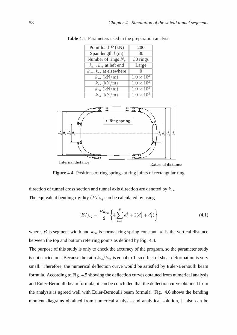
58 Chapter 4. Simulation of the shield tunnel segments
Table 4.1: Parameters used in the preparation analysis
Point loadP (kN) 200Span lengthl (m) 30
Number of ringsNr 30 ringsken, kes at left end Large
ken, kes at elsewhere 0ksn (kN/m) 1.0× 10³
kss (kN/m) 1.0× 10³
krn (kN/m) 1.0× 10³
krs (kN/m) 1.0× 10³
d2d4d6d8
Ring spring
Internal distance External distance
d7d5d3d1
Figure 4.4: Positions of ring springs at ring joints of rectangular ring
direction of tunnel cross section and tunnel axis direction are denoted bykes.
The equivalent bending rigidity(EI)eq can be calculated by using
(EI)eq =Bkrn
2
{4
6∑i=1
d2i + 2(d2
7 + d28)
}(4.1)
where,B is segment width andkrn is normal ring spring constant.di is the vertical distance
between the top and bottom referring points as defined by Fig. 4.4.
The purpose of this study is only to check the accuracy of the program, so the parameter study
is not carried out. Because the ratiokrs/ksn is equal to 1, so effect of shear deformation is very
small. Therefore, the numerical deflection curve would be satisfied by Euler-Bernoulli beam
formula. According to Fig. 4.5 showing the deflection curves obtained from numerical analysis
and Euler-Bernoulli beam formula, it can be concluded that the deflection curve obtained from
the analysis is agreed well with Euler-Bernoulli beam formula. Fig. 4.6 shows the bending
moment diagrams obtained from numerical analysis and analytical solution, it also can be

4.4. Steps of study 59
-6
-5
-4
-3
-2
-1
0
1
0 5 10 15 20 25 30
Def
lect
ion
(m)
Distance from left end (m)
d1
d2
ave. deflection = (d1+d2)/2
Numerical results
Euler-Bernoulli beam formula
average deflection at the center of each ring
PEI
x 3
6x 2
2l( (
Figure 4.5: Deflection curve of cantileverbeam : rectangular ring case
-6000
-5000
-4000
-3000
-2000
-1000
00 5 10 15 20 25 30
Distance from left end (m)
Ben
ding
mom
ent (
kN-m
).
Analytical solution
Numerical Results
Figure 4.6: Bending moment diagram ofcantilever beam : rectangular ring case
concluded that the bending moment diagrams obtained from these two approaches are mostly
same. Conclusively, it confirms that this numerical analysis by using rigid segment spring
model can analyze the structural mechanics problems such as the longitudinal direction of
rectangular cross section tunnel.
4.4 Steps of study
As shown in Fig. 4.7, firstly the application to the full-scale segment loading test is carried
out in order to obtain the appropriate spring constants. Secondly, by using the same set of the
spring constants, the application to the actual segmental rings in construction site is carried
out by taking two conditions of loading, short and long-term conditions, into account. The
comparison between the observed data and numerical results can indicate the applicability of
the rigid segment spring model in the design of shield tunnel lining.
Note that the simulation of the full-scale segment loading test(first part) is carried out through
3 rings model and the simulation of actual segmental rings in site (second part) is carried out
through infinite ring analysis.

60 Chapter 4. Simulation of the shield tunnel segments
Application to the full-scale segment
loading test
compare analysis results with experimental results Obtain appropriate
spring parameters
short-term loading condition long-term loading condition
with subgrade reaction without subgrade reaction
Evaluate model
compare analysis results with experiment results
Application to the actual tunnel ring (in-situ)
Figure 4.7: Steps of study on the application of the rigid segment spring model to the actualsegments
4.5 Application to full-scale segment loading test
4.5.1 Outline of the loading test
In the loading test, the safety of the linings and the adequacy of the design method were eval-
uated by directly applying to single segments and full segmental rings loads that were near to
the design loads. Actually, loading tests of both composite segmental rings and DC segmental
rings were carried out but in this section only loading test of composite segmental rings will
be discussed. Loading test on composite segmental rings is shown in Fig. 4.8 and consisted of
three rings assembled and bolted together. The specification of composite segmental rings is
illustrated in Table 4.2.
Loads were applied to the composite segmental rings from eight directions. (see Figs. 4.8 and
4.9) First, 10 kN was applied by each load jack. After that supports were removed. Then, for
each step segmental rings were applied by the incremental 10% of maximum load of each load
jack. The number of loading steps were 10 steps. Each maximum load of each load jack is
shown in Fig. 4.9. This maximum load is nearly equivalent to the design loads. After each load
increment, the amounts of lining displacement, generated stresses of segment body and joints,
joint openings and offset length between adjacent rings were measured.
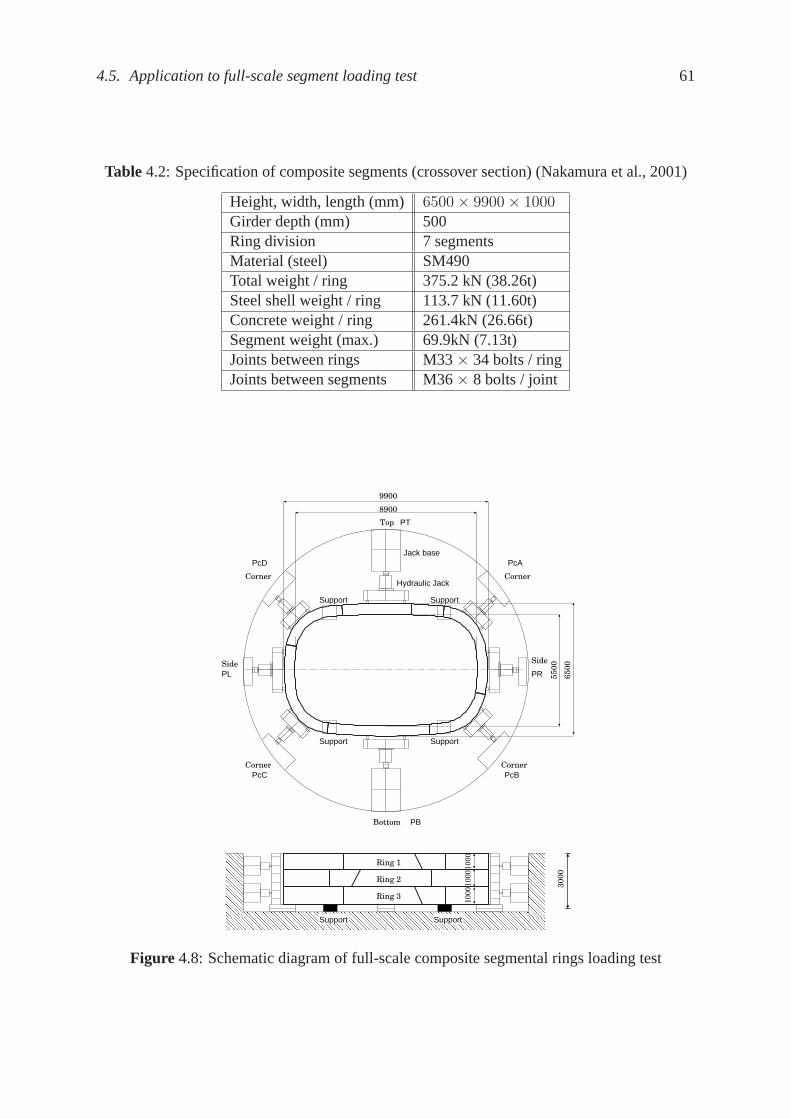
4.5. Application to full-scale segment loading test 61
Table 4.2: Specification of composite segments (crossover section) (Nakamura et al., 2001)
Height, width, length (mm) 6500× 9900× 1000Girder depth (mm) 500Ring division 7 segmentsMaterial (steel) SM490Total weight / ring 375.2 kN (38.26t)Steel shell weight / ring 113.7 kN (11.60t)Concrete weight / ring 261.4kN (26.66t)Segment weight (max.) 69.9kN (7.13t)Joints between rings M33× 34 bolts / ringJoints between segments M36× 8 bolts / joint
9900
8900
5500
6500
3000
Ring 1
Ring 2
Ring 3
Bottom
Corner
CornerCorner
Corner
Side Side
PB
PcBPcC
PL PR
PcAPcD
PTTop
Hydraulic Jack
Jack base
1000
1000
1000
Support
Support Support
Support
Support Support
Figure 4.8: Schematic diagram of full-scale composite segmental rings loading test

62 Chapter 4. Simulation of the shield tunnel segments
(3470 kN / 3 rings)
Top
(1764 kN / 3 rings)
Corner
(1764 kN / 3 rings)
Corner
(1764 kN / 3 rings)
Corner
(1764 kN / 3 rings)
Corner
(3470 kN / 3 rings)
Bottom
(2352 kN / 3 rings)
Side
(2352 kN / 3 rings)
Side
990m
m 2140mm
1620
mm
Figure 4.9: Loading condition for full-scale loading test
4.5.2 Joint behavior and spring constants
In this construction project, the beam-spring model was mainly used to design the shield tunnel
segments. The beam-spring model uses the rotational springKθ at the segment joint and the
shear springKs at the ring joint. To obtain the spring constants, the segment joint-bending test
and the ring joint-shear test were carried out to obtain the rotational spring constants and shear
spring constants, respectively(Kyoto Subway Tozai Line Rokujizo-Kita Construction Section,
2000). The behavior of each type of joints are explained as below:
Segment joint
According to Fig. 4.10, the segment joint behavior is not linear relationship between rotational
angle and bending moment. At the early state of loading, large increment of bending moment
for rotating segment joint is required due to the bearing of the adjacent segments. When this
early state is beyonded, instead of the bearing of adjacent ring, bolts carry load due to lower
increment of bending moment than the early state.
Ring joint
The shear force resistance of ring joint is shown in Fig. 4.11. The ring joint behavior is not a
linear relationship between displacement and shear force. At the early state of loading, shear
force is carried by the friction due to bolt tightening. The displacement of this early state is
very small. After the early state, the friction disappears and the space between bolt and hole

4.5. Application to full-scale segment loading test 63
Bending moment (kN m).
Rotational angle θ
K θ1+
K θ2+
K θ1−
K θ2−
450
-150
Figure 4.10: Bending moment vs. rotationalangle.
Shear force (kN)
δ (mm)
K s1
Ks2
Ks3
85
115
Figure 4.11: Shear force vs. displacement.
Table 4.3: Spring constants used in the beam-spring model
Segment joint (apply axial force) Ring joint (not apply axial force)Rotational spring constantKθ (kN ·m/rad) Shear spring constantKs (kN/m)
Kθ1 Kθ2 Ks1 Ks1 Ks1
Positive 7.5× 10⁵ Positive 3.7× 10⁵
Negative 3.7× 10⁵ Negative 1.0× 10⁵ 3.0× 10⁶ 1.0× 10⁴ 1.5× 10⁵
causes the additional displacement. Finally, shear force is resisted by the bolts themselves.
Table 4.3 illustrates the spring constants obtained from joint-bending test and ring joint-shear
test. Figs. 4.10 and 4.11 shows bending moment-rotational angle and shear force-displacement
curves, respectively.
In this study, the numerical analysis by using rigid segment spring model is carried out in order
to evaluate the applicability of the rigid segment spring model. The spring constants used in
analysis based on the spring constants used in the beam-spring model. However, positions and
number of each types of springs of rigid segment spring model are not the same as the beam-
spring model. In order to apply spring constants to rigid segment spring model, these spring
constants must be modified approximately as follows:
Normal segment spring constantksn : According to Fig. 4.12, the segment springs of rigid
segment model locate at the edges of segment joints. Because there are two springs locating at
one edge of segment joint, total spring force isF = 2ksn∆x and bending moment acting on
segment joint isM = Ft = 2k∆x. By using equationM = kθθ, therefore we can obtain
2ksn∆xt = Kθθ = Kθ∆x
t(4.2)

64 Chapter 4. Simulation of the shield tunnel segments
θ
θt
a
a
Section a-aF= 2k
M= Ft
..
2kKθ
x∆
x∆
Figure 4.12: Comparative diagram of normal segment spring and rotational spring
Thus,
ksn =Kθ
2t2(4.3)
Shear ring spring constantkrs : The number of ring springs of each segment is the same as
that of other segments. But actually the number of bolts connecting the adjacent rings together
is not the same. Therefore, according to Fig.4.13, a coefficientCi is supposed to modify the
shear ring spring constantkrs. Ci is defined as the ratio of the number of bolts (or ring springs
in beam-spring model) in parti to the number of ring springs in rigid segment spring model.
kmodrs = CiKs = Cikrs (4.4)
where,krs andkmodrs are shear ring spring constants before and after modification in rigid seg-
ment spring model, respectively, andKs is shear ring spring constant in beam-spring model.
Note that, at ring joint, there are only bolts at internal part of segment connecting two adjacent
rings together, the ring spring constants at external part of segment are initially set to be zero.
For example, seeing Fig. 4.13, at part 2, there are 2 springs at bottom for model and 4 bolts at
bottom for the actual ring, thusC2= 4/2 andkmodrs of each spring in part 2 is2Ks or 2krs.
Shear segment spring constantkss : Shear segment spring constant should be assumed to
be approximately 2.25 times(Kyoto Subway Tozai Line Rokujizo-Kita Construction Section,
2002a) of shear ring spring constant because at segment joint there is axial force acting on it.
However, actually there are 8 bolts connecting segment to the adjacent segment and there are
4 springs at segment joint in this study model. Therefore the shear segment spring constant of
each spring in this study model should be approximately 2 times. That meanskss is supposed
to be 4 times ofkrs.
Normal ring spring constant krn : krn is assumed to be constant and less thanksn suitably.

4.5. Application to full-scale segment loading test 65
Ring springBolt position
1 2 3 4
5
6
7
8910
11
12
13
14
Figure 4.13: Ring spring positions and bolt positions
Bending moment (kN m).
displacement (m)
k sn2 +450
-150
k sn1 +
k sn2 −
k sn1 −
Figure 4.14: Bending moment vs. dis-placement : segment normal spring con-stantksn
Bending moment (kN m).
displacement(m)
k rn Constant
Figure 4.15: Bending moment vs. dis-placement : ring normal spring constantkrn
Shear force (kN)
δ (mm)
k ss1
k ss2
k ss3
191
258
Figure 4.16: Shear force vs. Displace-ment : segment shear spring constantkss
Shear force (kN)
δ (mm)
k rs1
k rs2
k rs3
85
115
Figure 4.17: Shear force vs. Displace-ment : ring shear spring constantkrs

66 Chapter 4. Simulation of the shield tunnel segments
4.5.3 Condition and parameter settings
According to Fig. 4.13, the adjacent rings are connected by bolts which located at the internal
part of segments, thus the spring constants at external part of segments are supposed initially
to be zero(nodek = 21, 23, 25,..., 35 in Figs. 3.18 and 3.19). Moreover, at segment joint,
the normal segment spring constants of top springs are modified from the negative bending
moment rotational spring constants and spring constants of bottom springs are modified from
the positive bending rotational spring constants. The initial parameters modified by the method
described above, are summarized in Table 4.4.
The numerical analysis is carried out based on incremental analysis because spring constants
are not constant through loading as shown in Figs 4.14, 4.15, 4.16 and 4.17.
Table 4.4: Initial parameters for three segmental rings loading test analysis (Unit : kN/m)HHHHHHHHJoint
SpringNormal spring constant Shear spring constant
ip 1 ksn1 ksn2 kss1 ip1 kss2 ip2 kss3
+2 450 1.5× 10⁶ 7.4× 10⁵
Segment joint–3 150 7.4× 10⁵ 2.0× 10⁵ 1.35× 10⁷ 191 4.5× 10⁴ 258 6.75× 10⁵
ip krn1 krn2 krs15 ip1 krs2 ip2 krs3
+ none 1.0× 10⁵ 1.0× 10⁵
Ring joint4– none 1.0× 10⁵ 1.0× 10⁵ 3.0× 10⁶ 85 1.0× 10⁴ 115 1.5× 10⁵
1 ip : force or bending moment value at inflection point. Unit for normal spring is kN·m and for shear spring
is kN.
2 Positive bending moment
3 Negative bending moment
4 krs andkrn at the top part of ring joints are set to be zero.
5 Thiskrs is the value before modification (see Eq. (4.4))
4.5.4 Steps of incremental analysis
In order to simulate this full-scale loading test by using rigid segment-spring model, the incre-
mental analysis is carried out step by step as follows:
1. loads are applied increasingly from 0 kN/load jack up to 10 kN/load jack. The incremen-
tal analysis is repeated totally 100 times; then
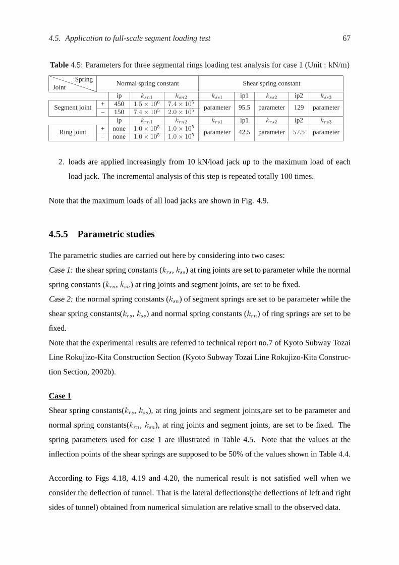
4.5. Application to full-scale segment loading test 67
Table 4.5: Parameters for three segmental rings loading test analysis for case 1 (Unit : kN/m)PPPPPPPPJoint
SpringNormal spring constant Shear spring constant
ip ksn1 ksn2 kss1 ip1 kss2 ip2 kss3
+ 450 1.5× 10⁶ 7.4× 10⁵
Segment joint– 150 7.4× 10⁵ 2.0× 10⁵ parameter 95.5 parameter 129 parameter
ip krn1 krn2 krs1 ip1 krs2 ip2 krs3
+ none 1.0× 10⁵ 1.0× 10⁵
Ring joint– none 1.0× 10⁵ 1.0× 10⁵ parameter 42.5 parameter 57.5 parameter
2. loads are applied increasingly from 10 kN/load jack up to the maximum load of each
load jack. The incremental analysis of this step is repeated totally 100 times.
Note that the maximum loads of all load jacks are shown in Fig. 4.9.
4.5.5 Parametric studies
The parametric studies are carried out here by considering into two cases:
Case 1:the shear spring constants (krs, kss) at ring joints are set to parameter while the normal
spring constants (krn, ksn) at ring joints and segment joints, are set to be fixed.
Case 2:the normal spring constants (ksn) of segment springs are set to be parameter while the
shear spring constants(krs, kss) and normal spring constants (krn) of ring springs are set to be
fixed.
Note that the experimental results are referred to technical report no.7 of Kyoto Subway Tozai
Line Rokujizo-Kita Construction Section (Kyoto Subway Tozai Line Rokujizo-Kita Construc-
tion Section, 2002b).
Case 1
Shear spring constants(krs, kss), at ring joints and segment joints,are set to be parameter and
normal spring constants(krn, ksn), at ring joints and segment joints, are set to be fixed. The
spring parameters used for case 1 are illustrated in Table 4.5. Note that the values at the
inflection points of the shear springs are supposed to be 50% of the values shown in Table 4.4.
According to Figs 4.18, 4.19 and 4.20, the numerical result is not satisfied well when we
consider the deflection of tunnel. That is the lateral deflections(the deflections of left and right
sides of tunnel) obtained from numerical simulation are relative small to the observed data.

68 Chapter 4. Simulation of the shield tunnel segments
0
0.001
0.002
0.003
0.004
0.005
0.006
0.007
0.008
0.009
0.01 0.1 1 10
6.1mm
Rig
ht s
ide
defl
ectio
n (m
)
Numerical results
Right side deflection from experiment
/ksn1krs1
Figure 4.18: Lateral deflection vs.krs1/ksn1 (case 1)
0
0.02
0.04
0.06
0.08
0.1
0.12
0.14
0.01 0.1 1 10
15.5mm
Cro
wn
defl
ectio
n (m
)
krs1 ksn1/
Numerical resultsCrown deflection from experiment
Figure 4.19: Crown deflection vs.krs1/ksn1 (case 1)
-4
-3
-2
-1
0
1
2
3
4
-6 -4 -2 0 2 4 6
-15.5(-13.7)
14.5(11.3)
6.1(1.11)
-5.5(-1.12)
Unit:mmRing 1
x
y
experimental value( numerical value )
-4
-3
-2
-1
0
1
2
3
4
-6 -4 -2 0 2 4 6
-15.5(-12.4)
14.5(10.4)
6.1(1.04)
-5.5(-1.18)
Unit:mmRing 2
x
y
experimental value( numerical value )
Figure 4.20: Deformation of segmental rings whenkrs1/ksn1 = 0.1 (case 1)
In order to obtain more lateral deflection,segment joint should set to be more flexible to rotate.
This means normal spring constants would be set to smaller. This is the basic concept of case
2.
Case 2
In order to consider how segmental rings deform when segment joints allowed to rotate easier,
normal spring constants (ksn) of segment springs are set to be parameterwhile the shear spring
constants (krs, kss) and the normal spring constants (krn) of ring springs are set to be fixed. The
spring parameters are shown in Table 4.6.
According to Figs 4.21 and 4.22, when ratiokrs1
ksn1
= 6.66 we obtained the good result. Both of
the vertical deflection of tunnel crown and the lateral deflection of tunnel springline obtained
from analysis are very close to the observed data. Fig 4.23 shows the deformation of segmental
rings at optical spring constants. Not only deflection but also bending moment of segmental
rings are satisfied with the observed data as illustrated in Fig. 4.24. Fig 4.25 shows the axial

4.5. Application to full-scale segment loading test 69
Table 4.6: Parameters for three segmental rings loading test analysis for case 2 (Unit : kN/m)PPPPPPPPJoint
SpringNormal spring constant Shear spring constant
ip ksn1 ksn2 kss1 ip1 kss2 ip2 kss3
+ 450 parameter parameterSegment joint– 150 parameter parameter
1.35× 10⁶ 95.5 4.5× 10³ 129 6.75× 10⁵
ip krn1 krn2 krs1 ip1 krs2 ip2 krs3
+ none 1.0× 10⁵ 1.0× 10⁵
Ring joint– none 1.0× 10⁵ 1.0× 10⁵ 3.0× 10⁵ 42.5 1.0× 10³ 57.5 1.5× 10⁴
0
0.002
0.004
0.006
0.008
0.01
0.012
0.014
0.016
0.018
0.02
0.022
0.1 1 10 100
righ
t sid
e de
flec
tion
(m)
6.1 mm
krs1 ksn1/
Ave. right side deflection from experiment
Numerical result
6.66
Figure 4.21: Lateral deflection vs.krs1/ksn1 (case 2:krs1/ksn1 = 6.66)
0.005
0.01
0.015
0.02
0.025
0.03
0.035
0.1 1 10 100
crow
n de
flec
tion
(m)
15.5 mm
Ave. crown deflectionfrom experiment
Numerical result
6.66krs1 ksn1/
Figure 4.22: Crown deflection vs.krs1/ksn1 (case 2:krs1/ksn1 = 6.66)
force (hoop force) of segmental rings and it can be seen that the observed data are too varied but
there are some points which satisfied by the numerical results. Table 4.7 shows the parameters
used in the optimal case.
Table 4.7: Parameters for three segmental rings loading test analysis for optimal case (Unit :kN/m)PPPPPPPPJoint
SpringNormal spring constant Shear spring constant
ip ksn1 ksn2 kss1 ip1 kss2 ip2 kss3
+ 450 4.5× 10⁴ 2.22× 10⁴
Segment joint– 150 2.22× 10⁴ 6.0× 10³ 1.35× 10⁶ 95.5 4.5× 10³ 129 6.75× 10⁵
ip krn1 krn2 krs1 ip1 krs2 ip2 krs3
+ none 1.0× 10⁵ 1.0× 10⁵
Ring joint– none 1.0× 10⁵ 1.0× 10⁵ 3.0× 10⁵ 42.5 1.0× 10³ 57.5 1.5× 10⁴

70 Chapter 4. Simulation of the shield tunnel segments
-4
-3
-2
-1
0
1
2
3
4
-6 -4 -2 0 2 4 6
-15.4 (-14.8)
5.9 (6.1)
14.3(-12.5)
-5.5 (-4.7)
experimental value(numerical value)
Unit:mm
x
y
Ring 1
-4
-3
-2
-1
0
1
2
3
4
-6 -4 -2 0 2 4 6
-15.6 (-13.7)
6.3 (5.6)
14.5(12.2)
-5.4 (-4.3)
Unit:mm
x
y
Ring 2
experimental value(numerical value)
Figure 4.23: Deformation of segmental rings whenkrs1/ksn1 = 6.66 (case 2)
-4
-2
0
2
4
-6 -4 -2 0 2 4 6
725(733)
740(633)
-552(-722)
-399(-335)
610(895)
627(976)
-465(-493)
-359(-372)
experiment value(numerical value)
Unit : kN m.Ring 1
-4
-2
0
2
4
-6 -4 -2 0 2 4 6
674(600)
680(789)
-310(-386)
-762(-751)
586(1055)
662(882)
-268(-317)
-601(-934)
Unit : kN m.
experiment value(numerical value)
-208(-120)
-275(-818)
Ring 2
Figure 4.24: Bending moment diagram whenkrs1/ksn1 = 6.66 (case 2)
-6
-4
-2
0
2
4
6
-8 -6 -4 -2 0 2 4 6 8
-1381(-837) -421
(-831)
-1049(-1026)
-3224(-1240)
-809(-755)
-621(-740)
-2747(-914)
-2215(-1197)
Unit : kN
experiment value(numerical value)
-1645(-920)
-1715(-1066)
Ring 2
-6
-4
-2
0
2
4
6
-8 -6 -4 -2 0 2 4 6 8
-1134(-865)
-1434(-869)
-2772(-1124)
-3301(-971)
-393(-773)
-1254(-791)
-1995(-1106)
-2624(-1000)
experiment value(numerical value)
Unit : kNRing 1
Figure 4.25: Hoop force diagram whenkrs1/ksn1 = 6.66 (case 2)

4.6. Application to in-situ segmental rings 71
101.0 kN/m2
168.7 kN/m2
101.0 kN/m2
184.3 kN/m2
14.34 kN/m
92.0 kN/m2
92.0 kN/m2
186.4 kN/m2
303 kN 377 kN
309 kN380 kN
101.0 kN/m2
168.7 kN/m2
Ground reaction
Figure 4.26: Loading condition in short-term including ground reaction
4.6 Application to in-situ segmental rings
Applications of the rigid segment spring model to the in-situ segment ring are carried out,
using the optimal spring parameters obtained from the previous section (Section 4.5). Both
short-term loading condition and long-term loading condition are considered to evaluate the
applicability of this model for design of the shield tunnel lining.
4.6.1 Short-term loading
Loading condition for short-term condition is shown in Fig. 4.26(Kyoto Subway Tozai Line
Rokujizo-Kita Construction Section, 2003). This load condition was modified from the in-situ
earth pressure measurement. The reaction forces,acting on the lining, induced by two support
columns removal, will be added in the analysis while ground reaction will be considered also.
We considered the case that there are only compressive reaction from ground i.e., consider only
the reaction springs located on the both lateral sides of segmental ring.
Parameter setting
The tunnel passes through gravel of the upper diluvial beds(including sand and clay partially).
N-value ranges from 20 to over 50. According to page 46 of literature (Tunnel engineering

72 Chapter 4. Simulation of the shield tunnel segments
8.39 m8.39 m
10 springs 10 springs
Figure 4.27: Length of ground reaction spring distributed on both sides of segmental ring
committee, 2003), for N-value over than 30 soil, the ground reaction spring constant is approx-
mimately in the range of 30-50 MN/m3. The tension ground reaction spring is ignored and only
compression ground reaction springs are considered. According to Fig. 4.27, then ground reac-
tion springs are placed along the circumferential length of each lateral side of segmental ring.
By modifying these ground reaction spring constants to the analysis model where there are 10
reaction springs along the circumferential length of the each lateral side of segmental ring i.e.,
each side length=8.39 m. Thus, for this analysis, three different ground spring constants (kes
andken) i.e., 25000, 35000 and 42000 kN/m for each spring, are used.
Results and discussions
Ring deformation
According to Figs. 4.28, 4.29 and 4.30, these figures shows the deformation of rings 1 and 2 for
each ground reaction spring constant. It is found that the deformation obtained from numerical
analysis agrees with the deformation measured in construction site. As ground reaction spring
constant is higher, the deformation of ring becomes smaller.
Bending moment and hoop force
Figs. 4.31, 4.32 and 4.33 illustrate the bending moment diagram for each case of ground
reaction spring constant. It is found that there is no significant difference in bending moment
among these three cases. The bending moment along the both sides of segment are fairly
satisfied with the the measured data in construction site. At the crown and bottom of ring,
however, the bending moment obtained from the numerical analysis is higher than the measured
data in construction site.

4.6. Application to in-situ segmental rings 73
For the hoop force, Figs. 4.34, 4.35 and 4.36, the measured data are very varied and the
hoop force obtained from the numerical analysis are quite lower than the the measured data.
However, there are good agreements at some positions i.e., at the bottom of ring 1 and the left
side of both rings, where the average hoop force is approximately equal to 1000 kN.
Offset length between adjacent segments
Table 4.8 shows the offset length between the adjacent segments. It is noted that the ground
reaction spring constant 25000, 35000 and 42000 kN/m are used for case 1, case 2 and case 3,
respectively. The number of segment joint is shown in Fig. 4.37. From table 4.8, we can see
that the offset length obtained from numerical analysis is larger than the measured data. This
result can be explained as follows:
The rigid segment spring model assumed the segment as the rigid body where there is no
strain within the body, but the actual segment may be elastic body. According to Fig. 4.38,
for both elastic and rigid segments, the reference point P on segment 2 displaces to point P′
with the displacementvp. For rigid segment (Fig. 4.38(a)), the displacementvp is equal to the
summation of the displacementv1 and the offset lengthlr of segment joint. However, for elastic
segment (Fig. 4.38(b)),vp is equal to the summation of the displacementv1, offset lengthle
of segment joint and the elastic deformationue of segment 2. This explanation can be written
mathematically as
vp =
Rigid segment︷ ︸︸ ︷v1 + lr =
Elastic segment︷ ︸︸ ︷v1 + le + ue (4.5)
If the elastic deformationue is assumed positively, then
lr > le (4.6)
which indicates that the offset length of rigid segment case is larger than that of elastic segment.
4.6.2 Long-term loading
The earth pressure distribution acting on the lining will be changed due to the lining defor-
mation. The long-term loading condition, as shown in Fig. 4.39, was obtained by averaging
the measured earth pressure on site for two months after support removal(Kyoto Subway Tozai

74 Chapter 4. Simulation of the shield tunnel segments
-4
-3
-2
-1
0
1
2
3
4
-6 -4 -2 0 2 4 6
-18.3 (-17.4)
2.4 (4.2)
7.7(10.8)
-2.4 (-4.8)
In situ value(numerical value)
Unit:mmRing 1
x
y
-4
-3
-2
-1
0
1
2
3
4
-6 -4 -2 0 2 4 6
-18.3 (-17.4)
2.4 (4.7)
7.7(11.0)
-2.4 (-4.2)
Unit:mm
x
y
In situ value(numerical value)
Ring 2
Figure 4.28: Cross-sectional deformation forken = kes = 25000 kN/m (short term)
-4
-3
-2
-1
0
1
2
3
4
-6 -4 -2 0 2 4 6
-18.3 (-15.7)
2.4 (3.3)
7.7(10.0)
-2.4 (-3.7)
Unit:mm
In situ value(numerical value)
Ring 1
x
y
-4
-3
-2
-1
0
1
2
3
4
-6 -4 -2 0 2 4 6
-18.3 (-15.5)
2.4 (3.68)
7.7(10.0)
-2.4 (-3.27)
Unit:mm
In situ value(numerical value)
Ring 2
x
y
Figure 4.29: Cross-sectional deformation forken = kes = 35000 kN/m (short term)
-4
-3
-2
-1
0
1
2
3
4
-6 -4 -2 0 2 4 6
-18.3 (-14.7)
2.4 (2.93)
7.7(9.58)
-2.4 (-3.18)
Unit:mm
In situ value(numerical value)
Ring 1
x
y
-4
-3
-2
-1
0
1
2
3
4
-6 -4 -2 0 2 4 6
-18.3 (-14.5)
2.4 (3.14)
7.7(9.64)
-2.4 (-2.90)
Unit:mm
In situ value(numerical value)
Ring 2
x
y
Figure 4.30: Cross-sectional deformation forken = kes = 42000 kN/m (short term)

4.6. Application to in-situ segmental rings 75
-4
-2
0
2
4
-6 -4 -2 0 2 4 6
456(834)
575(733)
-585(-1135)
13(-353)
305(1041)
426(1248)
-282(-960)
7(-477)
in situ value(numerical value)
Unit : kN m.596
(940)
385(1335)
-95(-640)
-482(-590)
Ring 1
-4
-2
0
2
4
-6 -4 -2 0 2 4 6
366(707)
298(874)
-109(-472)
-244(-943)
573(1199)
602(1057)
-240(-340)
-505(-1100)
in situ value(numerical value)
Unit : kN m.441
(948)
575(1318)
-727(-570)
-427(-620)
Ring 2
Figure 4.31: Bending moment diagram forken = kes = 25000 kN/m (short term)
-4
-2
0
2
4
-6 -4 -2 0 2 4 6
456(773)
575(699)
-585(-1105)
13(-343)
305(1033)
426(1263)
-282(-927)
7(-485)
in situ value(numerical value)
Unit : kN m.596
(892)
385(1339)
-95(-634)
-482(-582)
Ring 1
-4
-2
0
2
4
-6 -4 -2 0 2 4 6
366(685)
298(833)
-109(-483)
-244(-914)
573(1207)
602(1043)
-240(-338)
-505(-1089)
in situ value(numerical value)
Unit : kN m.441
(915)
575(1315)
-727(-576)
-427(-624)
Ring 2
Figure 4.32: Bending moment diagram forken = kes = 35000 kN/m (short term)
-4
-2
0
2
4
-6 -4 -2 0 2 4 6
456(789)
575(714)
-585(-1091)
13(-339)
305(1030)
426(1261)
-282(-924)
7(-484)
in situ value(numerical value)
Unit : kN m.596
(907)
385(1335)
-95(-621)
-482(-581)
Ring 1
-4
-2
0
2
4
-6 -4 -2 0 2 4 6
366(697)
298(838)
-109(-481)
-244(-893)
573(1207)
602(1040)
-240(-315)
-505(-1047)
in situ value(numerical value)
Unit : kN m.441
(922)
575(1313)
-727(-564)
-427(-585)
Ring 2
Figure 4.33: Bending moment diagram forken = kes = 42000 kN/m (short term)

76 Chapter 4. Simulation of the shield tunnel segments
-6
-4
-2
0
2
4
6
-8 -6 -4 -2 0 2 4 6 8
-1957(-1033)
-940(-1038)
-1659(-1215)
-3160(-964)
-553(-750)
431(-745)
-441(-1296)
Unit : kN -2532
(-1019)
-1050(-730)
498(-1046)
-730(-1110) in situ value
(numerical value)
Ring 1
-1545(-1127)
-6
-4
-2
0
2
4
6
-8 -6 -4 -2 0 2 4 6 8
-1413(-744)
233(-1014)
-1968(-1010)
-1756(-1120)
-56(-1271)
-1736(-957)
-1460(-1184)
Unit : kN
1261(-996) -2171
(-1090)-861
(-1026) in situ value(numerical value)
-1316(-738)
-2046(-723)
Ring 2
Figure 4.34: Hoop force diagram forken = kes = 25000 kN/m (short term)
-6
-4
-2
0
2
4
6
-8 -6 -4 -2 0 2 4 6 8
-1957(-1072)
-940(-1076)
-1659(-1208)
-3160(-963)
-553(-760)
431(-754)
-441(-1298)
-1545(-1134)
Unit : kN -2532
(-1058)
-1050(-740)
498(-1035)
-730(-1110) in situ value
(numerical value)
Ring 1
-6
-4
-2
0
2
4
6
-8 -6 -4 -2 0 2 4 6 8
-1968(-1073)
-1756(-1145)
-56(-1279)
-1736(-963)
-1460(-1199)
Unit : kN
1261(-1058) -2171
(-1140)-861
(-1030) in situ value(numerical value)
-1316(-777)
-2046(-762)
-1413(-784)
233(-1076)
Ring 2
Figure 4.35: Hoop force diagram forken = kes = 35000 kN/m (short term)
-6
-4
-2
0
2
4
6
-8 -6 -4 -2 0 2 4 6 8
-1957(-1127)
-940(-1131)
-1659(-1224)
-3160(-981)
-553(-791)
431(-784)
-441(-1302)
-1545(-1161)
Unit : kN -2532
(-1113)
-1050(-770)
498(-1046)
-730(-1121) in situ value
(numerical value)
Ring 1
-6
-4
-2
0
2
4
6
-8 -6 -4 -2 0 2 4 6 8
-1968(-1119)
-1756(-1166)
-56(-1272)
-1736(-969)
-1460(-1201)
Unit : kN
1261(-1104) -2171
(-1103)-861
(-1026) in situ value(numerical value)
-1316(-790)
-2046(-777)
-1413(-798)
233(-1122)
Ring 2
Figure 4.36: Hoop force diagram forken = kes = 42000 kN/m (short term)

4.6. Application to in-situ segmental rings 77
Table 4.8: Offset length between adjacent segments of Ring 1(unit:mm)
Position observed numerical resultcase 1 case 2 case3
➀ 2 6 6 6➁ 2 7 7 7➂ 2 0 0 0➃ 4 7 7 7➄ 2 8 8 8➅ 5 0 0 0➆ 4 8 8 8
5
3
4
6
1 27
Figure 4.37: Numbering of positions of segment joints
Undeformed ring
Segment 1Segment 2
v1
l e
Deformed ring
h
vp
Segment 1Segment 2
v1
l r
Deformed ring
h
vp
(a) Rigid segment
(b) Elastic segment
Undeformed ring
P
P’
P
P’ue
rigid segment line
Figure 4.38: Comparison between rigid and elastic segments

78 Chapter 4. Simulation of the shield tunnel segments
54.7 kN/m2
128.3 kN/m2
201.4 kN/m2
107.3 kN/m2
128.3 kN/m2
107.3 kN/m2
132.1 kN/m2
14.34 kN/m
201.4 kN/m2
Figure 4.39: Long-term loading condition(Kyoto Subway Tozai Line Rokujizo-Kita Construc-tion Section, 2002a)
Line Rokujizo-Kita Construction Section, 2002a). The same spring parameters as those of
short-term loading case are used without ground reaction springs.
Fig. 4.40 shows the deformation of segmental rings 1 and 2. It can be seen that the deformation
of segmental rings are very small compared to the measured data on site and deformation
obtained from short-term loading condition. The long-term loads were measured at the stable
state of segmental ring, hence segmental ring will not be deformed much. With this reason, the
small deformation obtained from this analysis should be reasonable.
For bending moment and hoop force diagrams (see Fig. 4.41 and 4.42), the numerical results
are also small compared to those of the short-term loading condition.
4.7 Conclusions
The rigid segment spring model for analyzing the actual shield tunnel lining by considering the
fact that the adjacent segments are not overlapped on each other was developed. Moreover, the
methodology for analyzing the infinite segmental rings by considering only two representative
rings was also proposed.
The parametric studies in order to determine the appropriate spring constants were carried out
first by simulating the large-scale loading test on three segmental rings. The first case in which
the shear spring constants at ring joints were varied and normal spring constants are fixed, was
carried out. No any set of spring constants was found to make the good agreement between
the computed deformation and observed deformation i.e., the computed vertical deformation

4.7. Conclusions 79
-4
-3
-2
-1
0
1
2
3
4
-6 -4 -2 0 2 4 6
-18.3[-15.7](-0.064)
7.7[10.0](0.025)
2.4[3.3](0.0)
-2.4[-3.7](0.0)
Unit:mmRing 1
x
y
-4
-3
-2
-1
0
1
2
3
4
-6 -4 -2 0 2 4 6
-18.3[-15.5](-0.06)
7.7[10.0](0.025)
2.4[3.68](0.0)
-2.4[-3.27](0.0)
Unit:mmRing 2
x
y
In situ value[Short-term](Long-term)
In situ value[Short-term](Long-term)
*** k enk es and for short-term loading condition are 35000 kN/m
Figure 4.40: Cross-section deflection (long term)
-4
-2
0
2
4
-6 -4 -2 0 2 4 6
Ring 1
-4
-2
0
2
4
-6 -4 -2 0 2 4 6
Ring 2
in situ data
Long-term Short-term
in situ data
Long-term Short-term
*** k enk es and for short-term loading condition are 35000 kN/m
Figure 4.41: Bending moment diagram (long term)
-6
-4
-2
0
2
4
6
-8 -6 -4 -2 0 2 4 6 8
Ring 1
-6
-4
-2
0
2
4
6
-8 -6 -4 -2 0 2 4 6 8
Ring 2
in situ data
Long-term
Short-term
in situ data
Long-term
Short-term
*** k enk es and for short-term loading condition are 35000 kN/m
Figure 4.42: Hoop force diagram (long term)

80 Chapter 4. Simulation of the shield tunnel segments
of the crown and bottom of rings and computed horizontal deformation of lateral sides of rings
are not satisfied the observed deformation when the same set of spring constants is used. The
second case was subsequently carried out in order to allow the segment joint more easily to
rotate. The normal spring constants are varied while the shear spring constants are fixed. The
appropriate set of spring constants was found when the ratiokrs1/ksn1 is approximately 6.66.
By using this appropriate set of spring constants in the application of the rigid segment spring
model to the actual segmental rings, the two cases of loading conditions, short-term and long-
term conditions, were carried out. From comparison between numerical results and observed
values from construction site, the deformation obtained from the short-term loading condition
are close to the observed valued. For the long-term loading condition, the deformation is almost
zero. This comparative results are reasonable because in the actual situation, the segmental
ring deformed due to the short-term loads and no further deformation occur when it reachs the
stable stage i.e., long-term condition. It can be concluded, therefore, that the rigid segment
spring model can be expected to apply in the design of shield tunnel lining if the appropriate
spring parameters can be obtained.

Part II
New Austrian Tunneling Method (NATM)
81


Chapter 5
Rigid-plastic finite element method
5.1 Introduction
A rigid-plastic finite element method, namely RPFEM, is recently considered as the effec-
tive tool to determine the critical strength of soil or rock structures such as dams, tunnels
and the foundations for the large structures, without the increase of the numerical errors which
is a problem in the conventional finite element method. This method is interpreted as an ex-
tension of the classical limit analysis of a frame structure to continuum, being based on the
upper-bound theorem in plasticity(Tamura, 1990). The critical state is obtained by minimizing
of the rate of internal plastic energy dissipation with respect to the kinematically admissible
velocity field under several linear constraint conditions(Tamura et al., 1984).
In this chapter, the theoretical basis for plasticity will be described followed by the stress-strain
rate relationships and the fundamental equations and boundary conditions for rigid-plastic anal-
ysis. The formulation of the finite element method will be also explained. Furthermore, the
methodology to include the effect of groundwater in the rigid-plastic finite element method
will be proposed.

84 Chapter 5. Rigid-plastic finite element method
σ σ
ε ε
a) Elasto-plastic model b) Rigid-plastic model
Hardening
Perfectly plastic
SofteningRigid
Plastic
A
B
C +
C 0
C -
A
B C
D
εe
εp
ε
Figure 5.1: Stress-strain relations: a) Elasto-plastic model and b) rigid-plastic model.
5.2 Theoretical basis for plasticity
5.2.1 Fundamental concept of plasticity
The fundamental concept of the elasto-plastic constitutive model is described first(Potts and
Zdrvkovic, 1999). Fig. 5.1a) shows the stress-strain relation for the elasto-plastic material.
On first material is loaded and deforms elastically and its stress-strain response travels along
the line AB. If the loading process is stopped before the stress in material reaches point B and
material is unloaded, the stress-strain response moves back down the line BA. Consequently,
as long as the loading does not cause the stress to reach point B, the material behaves in an
elastic manner and, when unloaded, returns to its original undeformed state, with no permanent
strains. For simplicity, the perfectly plastic material is described here. If the material is strained
beyondεe, to pointC0, the stress-strain curve passes through point B. Now the overall strain is
equal toε. At B, the yield stress is reached and the material becomes plastic. The stress remains
constant and equal to the yield stress. If the material is unloaded now it becomes elastic and
the stress-strain response moves along the lineC0D, which is parallel to the line BA. At point
D, the stress is zero but there is still strain in the material. This remaining strain is equivalent
to the strain experienced along the pathBC0 and called the plastic strain which is given by
εp = ε− εe (5.1)
where,εp andεe denote, respectively, plastic strain and elastic strain . Therefore, the material
does not return to its original shape. If the material is now reloaded, the stress-strain response

5.2. Theoretical basis for plasticity 85
f=kElastic zone
Plastic zone
σ
Figure 5.2: Yield surface.
σf=k
Plastic potential g = k
ε. ij
p
Yield surfaceσij
Figure 5.3: Plastic potential.
travels along the elastic pathDC0 until point C0 is reached and the material becomes plastic
again. Conclusively, the elastic paths AB andDC0 are reversible but the pathBC0 is not
reversible.
In addition, if the stress still increases after the yield stress is passed, this material is called
the strain-hardening material as shown by the pathABC+ in Fig. 5.1. For the strain-softening
material, as shown by the pathABC− in Fig. 5.1, the stress decreases when the yield stress is
reached.
In this dissertation, the elasto-plastic material is not considered but the rigid-perfectly plastic
material is mainly considered. As shown in Fig. 5.1b), the elastic component of strain is zero
in the limit and the material element is therefore rigid when stress is below the yield point. If
the limit state is reached, the material starts to flow with the constant stress.
5.2.2 Yield surface
The material exhibits the plastic deformations if and only if the stresses satisfy the yield con-
dition. This yield condition can be expressed by the yield function which is written as
f(σij) = k (5.2)
where,k is the non-negative material constant. This yield function is called the yield surface
which separates the elastic and plastic behavior in the stress space as shown in Fig. 5.2. Plastic
deformations can occur only iff(σij) = k. If f(σij) < k, there are no plastic deformations but
only the elastic deformations occur.

86 Chapter 5. Rigid-plastic finite element method
unstable
unstable
stable1
2
3
σ
ε
σ
ε
∆σ
∆ε(a) (b)
Figure 5.4: (a) Stress-strain relation for stable material , (b) Examples of stress-strain relationfor unstable material.
5.2.3 Plastic potential
Generally, the plastic deformation can be described by means of the plastic strain rateεpij. It is
now postulated that the plastic strain rate can be derived from a plastic potentialg, that depends
on the stresses only i.e.,g = g(σij), in such a way that the plastic strain rate can be obtained
by
εpij = λ
∂g
∂σij
if f(σij) = k (5.3)
where,λ is an undetermined constant.
Eq.(5.3) indicates that the strain rateεij is perpendicular to the plastic potentialg = k, as
shown in Fig. 5.3, and the stresses satisfy the yield surfacef = k.
5.2.4 Drucker’s stability postulate
Let us consider Fig. 5.4(a) showing the stress-strain relation of the stable material. It can be
seen that an additional loading∆σ > 0 gives rise to an additional strain∆ε > 0, with the
product∆σ∆ε > 0. This indicates that the additional stress∆σ does positive work. This kind
of material is calledstable. On the other hand, according to Fig. 5.4(b) (Drucker, 1959), the
additional stress of some parts of curve 1 and curve 3 does not do positive work and therefore
material which has the stress-strain behavior represented by curves 1 and 3 isunstablematerial.
According to the closed loading path shown in Fig. 5.5(Kobayashi, 2003), the path starts
from the initial stress stateσ0ij and crosses the initial yield surface atσ1
ij and then reaches the

5.2. Theoretical basis for plasticity 87
subsequent yield surface atσ1ij + δσij. After that the path returns back to the initial stress state.
The plastic deformations occurs betweenσ1ij andσ1
ij + δσij, the permanent strain remains in a
body if stress is removed to the initial state. Drucker (Drucker, 1951) gave a proposition that
the material is calledstableif and only if the net workWp done by stresses during this cycle
must be non-negative. This proposition is calledDrucker’s stability postulate. Net workWP
is determined by subtracting the work doneW0 by the initial stress from the total workWT
during the loading cycle, illustrated as the area surrounded by the thick arrow lines in Fig. 5.6.
Therefore, the net workWP can be calculated as
WP = WT −W0
=
∫ t3
t0
(σij(t)− σ0
ij
)εijdt
=
∫ t3
t0
(σij(t)− σ0
ij
) (εe
ij + εpij
)dt
=
∫ t2
t1
(σij(t)− σ0
ij
)εp
ijdt since∫
εeijdt = 0.
(5.4)
According to Drucker’s postulate, Eq.(5.4) can be written as
WP =
∫ t2
t1
(σij(t)− σ0
ij
)εp
ijdt ≥ 0. (5.5)
Since plastic strains materialise only att = t1, WP can be expanded as a Taylor series about
the neighborhood ofσij(t1), as follows:
WP (t) = (t− t1)(σij − σ0
ij
)εp
ij +(t− t1)
2
2!
[σij ε
pij +
(σij − σ0
ij
)εp
ij
]+ · · · . (5.6)
By assuming the value of(t2− t1) is small enough, only the first term of the right-hand side of
Eq.(5.6) is considered, then we have
(σij − σ0
ij
)εp
ij ≥ 0 if σij 6= σ0ij
σij εpij ≥ 0 if σij = σ0
ij.(5.7)
The inequality (5.7) is equivalent to the so-calledPrinciple of maximum plastic workproposed
by Hill (Hill, 1950). Consequently, the inequality(5.7) leads to the two important properties:

88 Chapter 5. Rigid-plastic finite element method
σij
0
(t= )t0
(t= )t3
.(t= )t1
Initial yield surface
Subsequent yield surface
σij
1
(t= )t2
σij
1σij+ δ
o
Figure 5.5: A closed loading path in relationto the yield surfaces.
σij
0
ε ij
0
σ
εδε ijε ij
0 +
δσijσij
1+
σij
1
δε ijε ij
0 +( )p
Figure 5.6: Schematic representation ofa stress cycle for stable material.
• Convexity of a yield surface : Yield surface must be convex in a stress space. The
definition of convexity is described in appendix B.
• Normality rule: If yield surface is smooth, direction of plastic strain rate coincides with
the direction of the outward normal vector of a yield surface if a yield surface is smooth.
This suggests that yield surfacef is equal to the plastic potentialg and according to
Eq.(5.3), we obtain
εpij = λ
∂f
∂σij
(5.8)
This rule can be called in another word, theassociated flow rule.
Generally, it has been found, by comparing theoretical results with experimental data, that for
metals very good agreements is obtained if the associated flow rule is considered. However,
many soils do not satisfy the associated flow rule because of the dilatancy, therefore, the non-
associated flow rule is introduced as the plastic potentialg does not coincide with the yield
function f . The relationship between the strain rate and the plastic potential is written as
Eq.(5.3).
5.2.5 Rate of plastic energy dissipation
For a given plastic strain rateεpij, the rate of specific plastic energy dissipationD(εp
ij) can be
defined as:

5.2. Theoretical basis for plasticity 89
.ε p
ijε p
ij
.
σ(1)
ij σ(2)
ij
O
Figure 5.7: Two states of stress corre-sponding to a plastic strain rate
.ε p
ij
σij
O
σij+ σij∆
ε p
ij
.∆+.ε p
ij
Figure 5.8: Increments of stress and plas-tic strain rate
D(εpij) = σij ε
pij (5.9)
in which σij denotes a stress on the yield surface associated with the plastic strain rateεpij
through the normality rule. It should be noted that all of plastic strain rates are not always
allowed to define the rate of energy dissipation. For example, in the case of the von-Mises
yield criterion,εpij with nonvanishing volumetric component never satisfies the associated flow
rule for any stressσij on the yield surface. Therefore some kind of constraints depending on
the adopted yield criterion must be imposed on choosing the plastic strain rate forD(εpij).
On the other hand, more than one stress states, sayσ(1)ij andσ
(2)ij , may correspond to a given
εpij when the yield surface contains a flat face or a line as some portion of it. ButD(εp
ij)
can be regarded as a single-valued function ofεpij since the difference(σ(1)
ij − σ(2)ij ) is always
perpendicular toεpij, as illustrated in Fig. 5.7.
It is easy to show the following properties ofD(εpij).
a) D(εpij) = σij ε
pij is homogeneous of degree-one ofεp
ij sinceσij is independent of the
magnitude ofεpij.
b) The variation ofD, denoted byδD, is calculated as
δD = σijδεpij (5.10)
, by showingδεpij = 0 which results from the normality rule (see Fig. 5.8).
c) D(εpij) is convex inεp
ij if it is continuously differentiable.
This can be proved as follows:

90 Chapter 5. Rigid-plastic finite element method
O
σij
(1)
σij
(2)
ε. ij
p(1)
ε. ij
p(2)
Figure 5.9: Two states of stress and strain rate corresponding to each state of stress
Let us consider the two states of stress and strain rate corresponding to each state of
stress; (σ(1)ij , ε
p(1)ij ) and (σ(2)
ij , εp(2)ij ), as shown in Fig. 5.9. According to the normality rule
or the principle of maximum plastic work, we obtain
σ(1)ij ε
p(1)ij ≥ σ
(2)ij ε
p(1)ij . (5.11)
Subtract both sides of inequality(5.11) byσ(2)ij ε
p(2)ij , we have
σ(1)ij ε
p(1)ij − σ
(2)ij ε
p(2)ij ≥ σ
(2)ij
(ε
p(1)ij − ε
p(2)ij
). (5.12)
Then,
D(εp(1)ij )−D(ε
p(2)ij ) ≥ ∇D(ε
p(2)ij )(ε
p(1)ij − ε
p(2)ij ) (5.13)
which satisfies the characterizations of differentiable convex functions shown by inequal-
ity (B.4) in appendix B.
5.3 Rigid-plastic material
5.3.1 Stress-strain rate relations (associated flow rule)
A rigid-plastic material is considered to obey the Drucker-Prager yield criterion:
f(σij) = −αI1 +√
J2 = k (5.14)
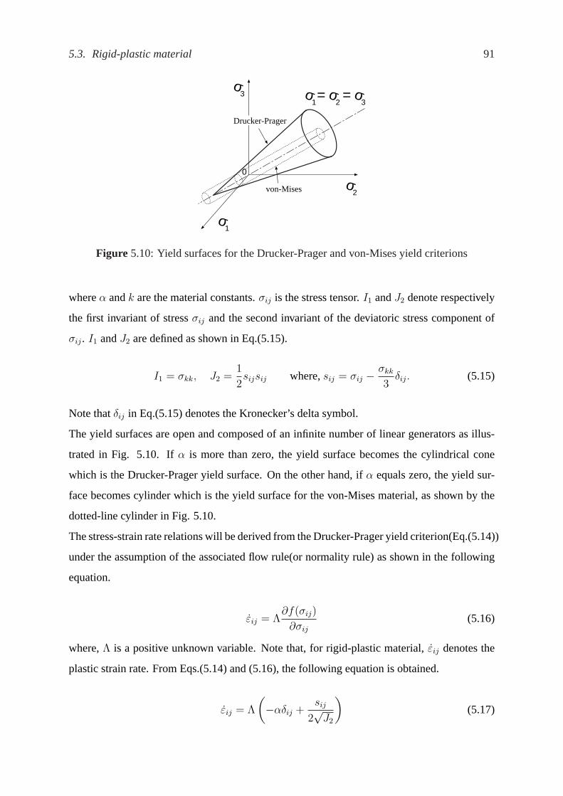
5.3. Rigid-plastic material 91
σ3
σ1
σ2
σ1
σ2
σ3
= =
0
Drucker-Prager
von-Mises
Figure 5.10: Yield surfaces for the Drucker-Prager and von-Mises yield criterions
whereα andk are the material constants.σij is the stress tensor.I1 andJ2 denote respectively
the first invariant of stressσij and the second invariant of the deviatoric stress component of
σij. I1 andJ2 are defined as shown in Eq.(5.15).
I1 = σkk, J2 =1
2sijsij where,sij = σij − σkk
3δij. (5.15)
Note thatδij in Eq.(5.15) denotes the Kronecker’s delta symbol.
The yield surfaces are open and composed of an infinite number of linear generators as illus-
trated in Fig. 5.10. Ifα is more than zero, the yield surface becomes the cylindrical cone
which is the Drucker-Prager yield surface. On the other hand, ifα equals zero, the yield sur-
face becomes cylinder which is the yield surface for the von-Mises material, as shown by the
dotted-line cylinder in Fig. 5.10.
The stress-strain rate relations will be derived from the Drucker-Prager yield criterion(Eq.(5.14))
under the assumption of the associated flow rule(or normality rule) as shown in the following
equation.
εij = Λ∂f(σij)
∂σij
(5.16)
where,Λ is a positive unknown variable. Note that, for rigid-plastic material,εij denotes the
plastic strain rate. From Eqs.(5.14) and (5.16), the following equation is obtained.
εij = Λ
(−αδij +
sij
2√
J2
)(5.17)

92 Chapter 5. Rigid-plastic finite element method
The magnitude of strain ratee is defined as
e =√
εij εij. (5.18)
Hence, using Eq.(5.17),
e2
= εij εij = Λ2
(3α2 +
1
2
)(5.19)
and
Λ =
√2√
6α2 + 1e (5.20)
are obtained. Then, Eq.(5.17) can be written as
εij
e=
√2√
6α2 + 1
(−αδij +
sij
2√
J2
). (5.21)
Multiplying δij into both sides of Eq.(5.21), we have
εkk +3√
2α√6α2 + 1
e = 0, (5.22)
whereεkk is defined as the volume change rate. Consequently, pulling the termεij out of the
parenthesis in Eq.(5.21), we obtain
εij
(δij +
3√
2α√6α2 + 1
εij
e
)= 0. (5.23)
This equation indicates that the strain rateεij is perpendicular to(δij + 3
√2α√
6α2+1
εij
e
). According
to Fig. 5.11 and the normality rule, the strain rateεij must be perpendicular to the generator
of the yield surface. Therefore, in case of the Drucker-Prager material, the direction of the
generator can be represented by(δij + 3
√2α√
6α2+1
εij
e
). To derive the stress-strain rate relation, the
stressσij is divided into the principal componentσ(1)ij and the indeterminate componentσ
(2)ij ,
i.e,
σij = σ(1)ij + σ
(2)ij . (5.24)
σ(1)ij locates in the dual cone and has the same direction as that ofεij, while σ
(2)ij locates in the

5.3. Rigid-plastic material 93
I1
f = k
σij
(1)
σij
(2)
.ij
ε
yield surface
σij
J2
0
Figure 5.11: Stress decomposition for the associated flow rule
conical yield surface and points to one of the generators of the yield surface. More precisely,
these stress components can be expressed by
σ(1)ij = G1
εij
eand, (5.25)
σ(2)ij = λ
(δij +
3√
2α√6α2 + 1
εij
e
)(5.26)
where,G1 is a positive coefficient which can be determined by the fact thatσ(1)ij fulfills the
yield condition
f(σ(1)ij ) = k. (5.27)
For the Drucker-Prager yield condition (Eq.(5.14)), it follows that
G1 =
√2k√
6α2 + 1. (5.28)
The indeterminate stress parameterλ is the unknown variable and will be determined after the
whole problem is solved.
Conclusively, the stressσij can be expressed as follows:
σij =
√2k√
6α2 + 1
εij
e+ λ
(δij +
3√
2α√6α2 + 1
εij
e
)
= (G1 + G2λ)εij
e+ λδij
(5.29)

94 Chapter 5. Rigid-plastic finite element method
in which
G2 =3√
2α√6α2 + 1
(5.30)
5.3.2 Stress-strain rate relations (non-associated flow rule)
The stress-strain rate relation based upon the associated flow rule often produces too large
volume expansion due to the dilatancy, when the large angle of internal friction is considered.
In order to decrease the effect of the dilatancy without changing the internal friction angle,
the non-associated flow rule was adopted. According to Fig. 5.12, stress is satisfied by the
yield criterion but the plastic potential is not the same as the yield surface, i.e., not parallel
to the generator of the Drucker-Prager yield surface. The plastic potential function for the
non-associated flow rule, given by
g(σij) = −αI1 +√
J2 = k (5.31)
is assumed to be the conical shape and any strain rateεij must be normal to this plastic poten-
tial. Note that the plastic potential given by Eq.(5.31) is similar to Eq.(5.14) but the material
constants,i.e.,α andk, are different. The condition for the normality to the potential is
εij = Λ∂g(σij)
∂σij
(5.32)
where,Λ is a positive unknown variable. By using similar procedure as the associated flow
rule, we haveεij
e=
√2√
6α2 + 1
(−αδij +
sij
2√
J2
)and, (5.33)
εkk +3√
2α√6α2 + 1
e = 0. (5.34)
The stress tensor is divided again into two components and the same forms are assumed as in
Eqs.(5.25) and (5.26):
σ(1)ij = G1
εij
e(5.35)
σ(2)ij = λ
(δij +
3√
2α√6α2 + 1
εij
e
). (5.36)
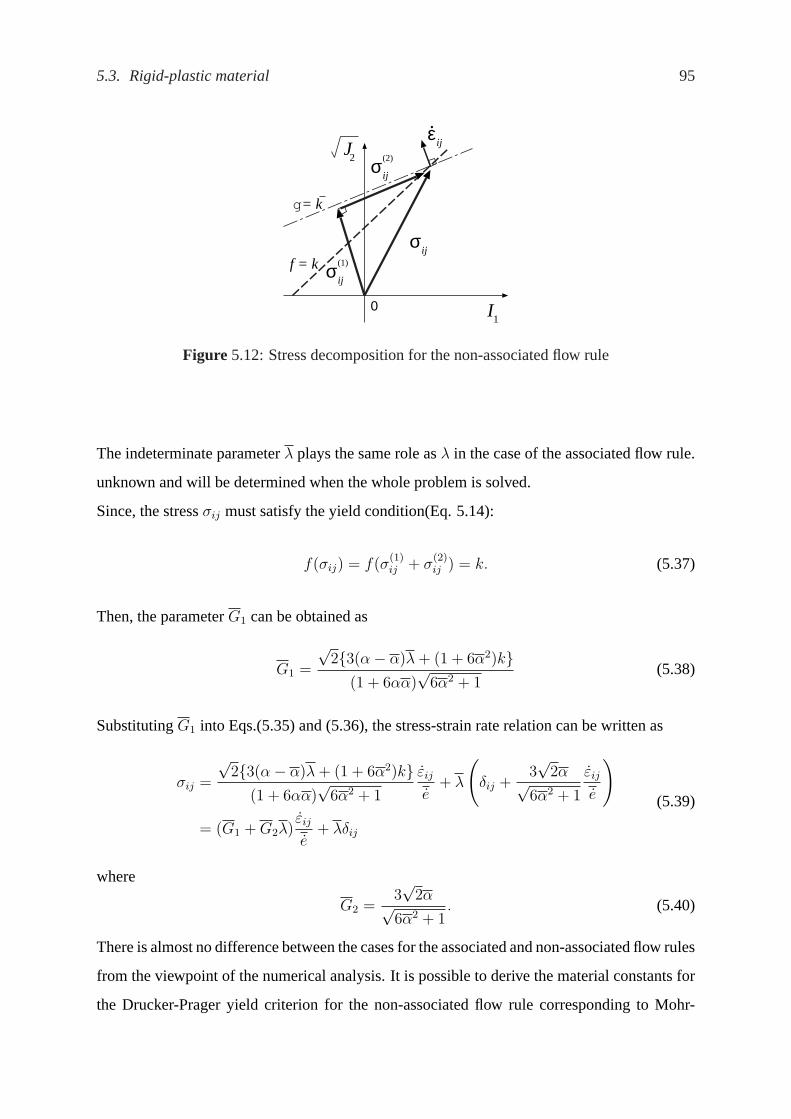
5.3. Rigid-plastic material 95
I1
f = k σij
(1)
σij
(2)
.ij
ε
σij
J2
g= k
0
Figure 5.12: Stress decomposition for the non-associated flow rule
The indeterminate parameterλ plays the same role asλ in the case of the associated flow rule.
unknown and will be determined when the whole problem is solved.
Since, the stressσij must satisfy the yield condition(Eq. 5.14):
f(σij) = f(σ(1)ij + σ
(2)ij ) = k. (5.37)
Then, the parameterG1 can be obtained as
G1 =
√2{3(α− α)λ + (1 + 6α2)k}
(1 + 6αα)√
6α2 + 1(5.38)
SubstitutingG1 into Eqs.(5.35) and (5.36), the stress-strain rate relation can be written as
σij =
√2{3(α− α)λ + (1 + 6α2)k}
(1 + 6αα)√
6α2 + 1
εij
e+ λ
(δij +
3√
2α√6α2 + 1
εij
e
)
= (G1 + G2λ)εij
e+ λδij
(5.39)
where
G2 =3√
2α√6α2 + 1
. (5.40)
There is almost no difference between the cases for the associated and non-associated flow rules
from the viewpoint of the numerical analysis. It is possible to derive the material constants for
the Drucker-Prager yield criterion for the non-associated flow rule corresponding to Mohr-

96 Chapter 5. Rigid-plastic finite element method
V
T-
i
Sσ
Su
Su
u i =0
u i = u i−
.
. .
f-
i
Figure 5.13: Considered rigid-plastic boundary value problem
Coulomb’s yield criterion in plane strain condition:
k =
3cα
tan φif φ > 0
c if φ = 0
(5.41)
α =
√(3 + 2r sin2 φ)−
√9 + 12r(1− r) sin2 φ
6r2(3 + sin2 φ)if r 6= 0
sin φ
3if r = 0
(5.42)
where
α = rα ( 0 ≤ r ≤ 1) (5.43)
andc andφ denote respectively the cohesion and the angle of internal friction of the Mohr-
Coulomb material.
It should be noted that whenr = 1, the non-associated flow rule becomes the same as the
associated flow rule.α in Eq.(5.42) can be reduced in the form:
α =sin φ√
3(3 + sin2 φ). (5.44)

5.4. Fundamental equations and boundary conditions for rigid-plastic analysis 97
5.4 Fundamental equations and boundary conditions for rigid-
plastic analysis
RegionV of a rigid-plastic material is divided into two disjointed subsetsSσ andSu as shown
in Fig. 5.13. The material is subjected to a body forcefi and a surface tractionTi on the stress
boundarySσ. The smooth velocity fieldui is defined at each point of the velocity boundarySu.
The external forces such asTi, fi are multiplied by the load factorµ under which the whole
region of the body begins to yield and flow with a constant rate of deformation. This steady
flow is governed by the equations of equilibrium:
−σij,j + µfi = 0 in V (5.45)
the stress boundary conditions:
−σijnj = µTi onSσ (5.46)
and the velocity boundary conditions:
Homogeneous velocity boundary conditions: ui = 0 onSu
Non-homogeneous velocity boundary conditions:ui = ui onSu
(5.47)
whereni denotes the outward unit normal onSσ. By adopting the small deformation theory,
the compatibility conditions can be written as
εij = −1
2(ui,j + uj,i) . (5.48)
5.5 Upper-bound theorem for rigid-plastic analysis
The concept of the upper-bound theorem is described below.
The loads, determined by equating the external rate of work to the internal rate of dissipation in
an assumed deformation mode(or velocity field) that satisfies: (a) velocity boundary condition
(Eq.(5.47)); and (b) strain and velocity compatibility conditions (Eq.(5.48)), arenot lessthan

98 Chapter 5. Rigid-plastic finite element method
the actual collapse load (Chen, 1975). A velocity field satisfying the above conditions has
been termed akinematically admissible velocityfield. The dissipation of energy in plastic flow
D(εpij) associated with such a field can be computed from the stress-strain rate relation.
According to the above-mentioned concept of the upper-bound theorem, assume that the exter-
nal forces(fi, Ti) be given and introduce the subsetKp (⊂ K):
Kp =
{(ui, εij) ∈ K|
∫
V
fiuidV +
∫
Sσ
TiuidS > 0
}(5.49)
For (ui,εij) ∈ Kp, define the load factorµ by
µ
{∫
V
fiuidV +
∫
Sσ
TiuidS
}=
∫
V
D(εij) dV =
∫
V
σij εij dV (5.50)
The upper-bound theorem states that
µ∗ ≤ µ (5.51)
whereµ∗ is the load factor at the limit state. To prove Eq.(5.51), we first compare Eq.(5.50)
with
µ∗{∫
V
fiuidV +
∫
Sσ
TiuidS
}=
∫
V
σ∗ij εijdV (5.52)
which represents the principle of virtual work for a kinematical field(ui,εij) and a equilibrium
systemµ∗(fi, Ti), σij∗. Subtracting Eq.(5.50) by Eq.(5.52), we obtain
(µ− µ∗){∫
V
fiuidV +
∫
Sσ
TiuidS
}=
∫
V
(σij − σ∗ij)εijdV (5.53)
Considering the definition ofKp and the principle of maximum plastic work(Eq.(5.7)), we
obtain Eq.(5.51).
5.6 Formulation of rigid-plastic finite element method(RPFEM)
5.6.1 Description of the problem
The formulation of rigid-plastic finite element method starts from defining the main problem
by considering the upper-bound theorem and some constraint conditions. According to section

5.6. Formulation of rigid-plastic finite element method(RPFEM) 99
5.5, it is understood thatµ∗ is searched as the minimum value ofµ defined as
µ =
∫
V
D(εij)dV∫
V
fiuidV +
∫
Sσ
TiuidS
(5.54)
by surveying all of the elements inKp.
Since a rigid-plastic material is rate-insensitive, it is possible to specify the magnitude of ve-
locity without loss of generality. Hence
∫
V
fiuidV +
∫
Sσ
TiuidS = 1 (5.55)
can be assumed. Furthermore, the constraint condition on strain rateεij i.e., Eq.(5.22) for
associated flow rule or Eq.(5.34) for non-associated flow rule, must be taken into account.
Also, if there is additional constraint condition on velocity field, it is added in the consideration
also.
As mentioned above, it can be concluded that the problem becomes equivalent to
Problem 1¶ ³
Minimize∫
VD(εij)dV
subject to ⇒ ∫V
fiuidV +∫
SσTiuidS = 1
⇒ Constraint condition on strain rateεij :
Eq.(5.22) for associated flow rule, or
Eq.(5.34) for non-associated flow rule
⇒ Additional constraint conditions :
a1iui = 0
a2iui = 0
a3iui = 0...
wherea1i, a2i, a3i, . . . are the coefficients for each constraint condition.
µ ´

100 Chapter 5. Rigid-plastic finite element method
5.6.2 Numerical procedure
According to the description on the rigid-plastic material mentioned in section 5.3 and the
concept of upper-bound theorem mentioned section 5.5, the unknown variables of the overall
problem are assigned differently as follows:
• velocities at limit stateui are assigned for each nodal point,
• the indeterminate magnitude of the isotropic stress componentλ or λ is assigned for each
element,
• the load factorµ which indicates the limit state and,
• other parameters associated to the additional constraint conditions.
Now, the above-mentioned problem 1 is investigated by the finite element technique. In this
dissertation, the isoparametric quadrilateral elements composed of 4 nodes and hexahedral
elements composed of 8 nodes are used in 2D and 3D analysis, respectively. The notation
necessary to formulate the rigid-plastic finite element analysis will be introduced as follows:
ue : vector of nodal velocities in each element
u : vector of all nodal velocities
σe : vector of stresses of an element defined as
σe =
{σxx, σyy, σxy}T for 2D analysis
{σxx, σyy, σzz, σxy, σyz, σzx}T for 3D analysis(5.56)
σ : vector of stresses of all elements
εe : vector of engineering strain rate of an element, defined as
εe =
{εxx, εyy, γxy}T for 2D analysis
{εxx, εyy, εzz, γxy, γyz, γzx}T for 3D analysis(5.57)
ε : vector of engineering strain rate of all elements

5.6. Formulation of rigid-plastic finite element method(RPFEM) 101
Ee : vector of tensorial strain rateεij of an element, defined as
Ee =
{εxx, εyy, εxy}T for 2D analysis
{εxx, εyy, εzz, εxy, εyz, εzx}T for 3D analysis(5.58)
F : vector of all nodal forces
Be : strain rate-velocity matrix for an element, defined as shown in the compatibility condi-
tion as
εe = Beue (5.59)
B : strain rate-velocity matrix defined as
ε = Bu (5.60)
Therefore, according to Eq.(5.59), the relationship between vector of engineering strain rate
for each elementεe and the vector of tensorial strain rateEe is written as
Ee = Qεe
= QBeue
(5.61)
in which, for 2D analysis
Q =
1 0 0
0 1 0
0 0 12
(5.62)
and for 3D analysis,
Q =
1 0 . . . . . . . . . 0
0 1 0 . . . . . . 0... 0 1 0 . . . 0...
... 0 12
0 0...
...... 0 1
20
0 0 0 0 0 12
. (5.63)

102 Chapter 5. Rigid-plastic finite element method
According to Eq.(5.18), the magnitude of strain ratee can be written as
e =√
εij εij
=
√uT
e BTe QBeue
(5.64)
The volume change rateεkk is also written as
εkk =
∫
V
δT Beue dV
= Leue
(5.65)
where the matrixLe is defined as
Le =
∫
V
δT Be dV (5.66)
and the Kroneckor’s delta vectorδ is written as
δ =
{1, 1, 0}T for 2D analysis
{1, 1, 1, 0, 0, 0}T for 3D analysis(5.67)
Furthermore, the vector of rates of volume changev of all elements is defined as
v = Lu (5.68)
in whichL consists ofLe of each element.
Therefore the problem 1 as mentioned above can be written in the matrix forms as follows:

5.6. Formulation of rigid-plastic finite element method(RPFEM) 103
Problem 2¶ ³
Minimize∫
VD(εij)dV
subject to ⇒ F T u = 1
⇒ Constraint condition on strain rateεij :
Lu + G2
∫V
edV = 0 for associated flow rule
Lu + G2
∫V
edV = 0 for non-associated flow rule
⇒ Additional constraint conditions :
A1u = 0
A2u = 0
A3u = 0...
whereAi is the constraint matrix for each additional constraint
condition.
µ ´
Note that the constraint conditions for strain rateεij are applied toeach element(not to all
element).
Supposeu be a solution of problem 2. It means
∫
V
D(u + ∆u) ≥∫
V
D(u)dV (5.69)
for an arbitrary∆u which satisfies
F T ∆u = 0 (5.70)(
LT + G2
∫
V
BT QB
eu
)T
∆u = 0 (5.71)
Ai∆u = 0 (5.72)
Remember Eq.(5.10) and we have
∆
∫
V
D(u) dV =
∫
V
σT ∆ε dV =
(∫
V
σT B dV
)∆u
=
(∫
V
BT σ(1) dV
)T
∆u = 0
(5.73)

104 Chapter 5. Rigid-plastic finite element method
in which the last equation is justified apparently since the isotropic component of stress does
no work for∆u which satisfiesLu + G2
∫V
edV = 0.
Now, a basic theorem in algebra thata system of linear equationAx = b has at least one
solutionx if and only ifbT y = 0 for an arbitraryy such thatAT y = 0, is taken into account.
The system of equations composed of Eqs.(5.70), (5.71) and (5.72) can be written as
F T
−(LT + G2
∫VBTQB
eu dV
)T
Ai
∆u =
0
0
0
(5.74)
where matrixA and∆u are supposed by(F T ,−
(LT + G2
∫VBTQB
eu dV
),AT
i
)and vec-
tor y, respectively. Also, according to Eq.(5.73),(∫
VBT σ(1) dV
)is supposed byb. Hence,
by considering the above-mentioned theorem on algebra, we can conclude thatAx = b , i.e.,
(F ,−(LT + G2
∫
V
BT QB
eu dV ), AT
i
)
µ
λ
ν
=
∫
V
BT σ(1) dV (5.75)
in whichλ is composed of the indeterminate stress parametersλ of all elements.
Finally, for non-associated flow rule, the system of equations of the overall problem can be
written as
{∫
V
(G1 + λG2)BT QB
edV
}u + LT λ−AT
i ν − µF = 0 (5.76)
F T u− 1 = 0 (5.77)
Lu + G2
∫
V
e dV = 0 (5.78)
Aiu = 0 (5.79)

5.6. Formulation of rigid-plastic finite element method(RPFEM) 105
where Eq.(5.76) is called the equations of equilibrium. Eqs.(5.77), (5.78) and (5.79) are the
constraint conditions. And for associated flow rule,
{∫
V
(G1 + λG2)BT QB
edV
}u + LT λ−AT
i ν − µF = 0 (5.80)
F T u− 1 = 0 (5.81)
Lu + G2
∫
V
e dV = 0 (5.82)
Aiu = 0 (5.83)
are obtained.
5.6.3 Newton-Raphson method
According to the above-mentioned system of equations,e is a nonlinear function of the ve-
locities u, therefore, the system of equations will be solved iteratively by using the Newton-
Raphson method.
Let us consider a non-linear function
f(x) = 0. (5.84)
To solve the above equation, the Newton-Raphson method requires the evaluation of both the
functionf(x) and the derivativef ′(x), at arbitrary pointsx(Press et al., 1992). The function
f(x) is approximately derived from Taylor series expansion of a function in the neighborhood
of pointx,
f(x + ∆x) = f(x) + ∆xf ′(x) + ∆x2f ′′(x)
2+ . . . = 0 (5.85)
If ∆x is small enough, the terms beyond linear are unimportant, hencef(x + ∆x) = 0 implies
∆x = − f(x)
f ′(x)or f ′(x)∆x = −f(x) (5.86)
To obtain the solution off(x) = 0, the iterative analysis is required. Let us start from the initial
x0. The next stepx1 is illustrated by
x1 = x0 + ∆x = x0 − f(x0)
f ′(x0)(5.87)

106 Chapter 5. Rigid-plastic finite element method
More generally,
xi+1 = xi + ∆x = xi − f(xi)
f ′(xi)(5.88)
can be written for stepi.
Newton-Raphson is not restricted to one dimension. The method readily generalizes to multiple
dimensions. According to the system of equations mentioned in the preceding section, the
unknown variables can be determined by
ui+1 = ui + ∆u
λi+1 = λi + ∆λ for non-associated flow rule
µi+1 = µi + ∆µ
νi+1 = νi + ∆ν
(5.89)
Note that, for associated flow rule,λ is considered instead ofλ.
For associated flow rule, determine the derivatives of Eqs.(5.80), (5.82), (5.81) and (5.83) and
make a system of equations following the form shown in Eq.(5.86) as
(G1 + G2λ)∫
V
(BTQB
e− BTQBuuTBTQB
e3
)dV LT + G2
∫VBTQB
eudV −F −AT
i
L + G2
(∫VBTQB
eudV
)T
−F T
−Ai
∆u
∆λ
∆µ
∆ν
=
−G1
∫VBTQB
edV −LT −G2
∫VBTQB
eudV F AT
i
−L−G2
(∫VBTQB
eudV
)T
F T
Ai
∆u
∆λ
∆µ
∆ν
+
F b
−1
(5.90)

5.7. RPFEM with consideration of groundwater 107
For non-associated flow rule, we obtain
(G1 + G2λ)∫
V
(BTQB
e− BTQBuuTBTQB
e3
)dV LT + G
⊗2
∫VBTQB
eudV −F −AT
i
L + G2
(∫VBTQB
eudV
)T
−F T
−Ai
∆u
∆λ
∆µ
∆ν
=
−G1
∫VBTQB
edV −LT −G2
∫VBTQB
eudV F AT
i
−L−G2
(∫VBTQB
eudV
)T
F T
Ai
∆u
∆λ
∆µ
∆ν
+
F b
−1
(5.91)
whereF b is a loading vector which is constant through the analysis and
G⊗2 =
3√
2α√
6α2 + 1
1 + 6αα(5.92)
Eqs.(5.90) and (5.91) are the system of linear equations. The unknown variables∆u, ∆λ (∆λ),
∆µ and∆ν of each step are determined by solving the system of linear equations. Further-
more, in order to guarantee the convergence of the iterated solutions, the positive constantη is
introduced to reduce the increment∆ for each step so that
ui+1 = ui + η∆u
λi+1 = λi + η∆λ for non-associated flow rule
µi+1 = µi + η∆µ
νi+1 = νi + η∆ν
(5.93)
For associated flow rule,λ is used instead ofλ.
5.7 RPFEM with consideration of groundwater
In this section, the methodology to include the groundwater into the rigid-plastic analysis is
described. The critical state of the soil structures is evaluated by determining the load factor
µ which magnifies the acceleration of gravityg. Therefore the actual collapse occurs under
the1g condition, if the obtained load factorµ is smaller than 1. This evaluation method has a

108 Chapter 5. Rigid-plastic finite element method
similar concept to that of the centrifugal modeling test. At the critical state, not only the unit
weight of soilγ but also the pore water pressurep is multiplied by the load factorµ.
To include the groundwater in the analysis, the following three factors are taken into account.
• Change in the total self-weight due to the change in the groundwater table.
• Change in the effective stress due to the change in the total self-weight and pore water
pressure.
• Strength of the ground due to the change in the effective stress.
5.7.1 Self-weight of soil
According to Fig. 5.14(a), the soil above the groundwater table is treated as the dry soil and its
unit weight is denoted by dry unit weightγd. On the other hand, the soil under the groundwater
table is considered as the saturated soil and its total unit weight is denoted by the saturated unit
weightγs. The unit weight of the soil element through which the groundwater table passes as
shown in Fig. 5.14(b), is estimated as follows:
γ = (1− αγ)γd + αγγs. (5.94)
In Eq.(5.94), the coefficientαγ is defined by Eq. 5.95.
αγ =Hc − ymin
ymax − ymin
(5.95)
whereymax and ymin denote the maximumy coordinate and minimumy coordinate of the
element, respectively, whileHc is the water head at the center of the element as shown in Fig.
5.14(b).
5.7.2 Pore water pressure
The distribution of the total water headH in the steady seepage state is determined in advance.
The pore water pressurep for each element can be calculated by averaging the pore water

5.7. RPFEM with consideration of groundwater 109
y
x
CL
D
µγd
Tunnel
p = 0
p = (Σ p )/4i
µγ
µγ s
p = (Σ p )/4
{
{
{i
, µp
, µp
, µp
p : pore water pressure
γ : unit weight of soil
µ : load factor
ground water table Hc
center
ymax
ymin
i
Hi
H : water head
(a)
(b)
Figure 5.14: Calculations of unit weight and pore water pressure
pressures of all 4 nodes as shown in the following equation.
pi =
γw(Hi − yi) if Hi ≥ yi
0 if Hi < yi
(5.96)
whereγw is the unit weight of water.yi andHi denote, respectively, they coordinate and the
water head of the nodal pointi. The pore water pressurep of each element is calculated by
p = (4∑
i=1
pi)/4. (5.97)
5.7.3 Effective stress
The effective stressσ′ij is equal to the total stressσij subtracted by the pore water pressurep,
as follows:
σ′ij = σij − µδijp (5.98)
whereδij is the Kronecker delta.
The rigid plastic finite element method with the consideration of groundwater is carried out by
considering the soil as non-homogenous soil i.e., the unit weight is varied by the groundwater
table. The important point is the effective stressσ′ij is considered in the stress-strain rate

110 Chapter 5. Rigid-plastic finite element method
relation based on the Drucker-Prager yield criterion (Eq.(5.29) or Eq.(5.39)) and the stress
tensor in the equations of equilibrium(Eq.(5.45)) is thetotal stresstensor. We can conclude the
above-mention point as follows:
Equations of equilibrium: σij,j + µf i = 0 (5.99)
whereσij is the total stresstensor andf i is the body force vector. Therefore, combining
Eq.(5.98) with Eq.(5.39), the total stress-strain rate relation for non-associated flow rule can be
written as
σij = (G1 + G2λ)εij
e+
(λ + µp
)δij (5.100)
Similarly, combining Eq.(5.98) with Eq.(5.29), the total stress-strain rate relation for associated
flow rule
σij = (G1 + G2λ)εij
e+ (λ + µp) δij (5.101)
is obtained.
Hence, the equations of equilibrium for associated flow rule, can be written as
{∫
V
(G1 + λG2)BT QB
edV
}u + LT (λ + µP )−AT
i ν − µF = 0
{∫
V
(G1 + λG2)BT QB
edV
}u + LT λ−AT
i ν − µ(F −LT P
)= 0
(5.102)
and that for non-associated flow rule is written as
{∫
V
(G1 + λG2)BT QB
edV
}u + LT λ−AT
i ν − µ(F −LT P
)= 0 (5.103)
whereP consists of the pore water pressurep of all elements.
Consequently,the systems of equations to be solved can be written by substitutingF in Eqs.(5.90)
or (5.91)by(F −LT P
).

Chapter 6
Numerical analysis of the tunnel stability in soft
clay
6.1 Introduction
T he safety of the tunnel construction in clay is usually considered into two problems.
Firstly, the stability of tunnel heading(area near the face) is necessary to be evaluated
for the safety of the construction. Secondly, the ground deformation due to the construction is
also required to be determined to prevent damage to existing surface or subsurface structures.
This chapter focuses on the first problem which is concerned with the determination of the
tunnel pressuresσT that are necessary to maintain the stability of the tunnel heading and of
the acceleration factor of the weight of soil mass that causes the collapse of the tunnel. The
stability of tunnel heading is evaluated by using the rigid-plastic finite element method and
the calculated tunnel pressureσT and calculated acceleration factorn (or load factorµ for
RPFEM) are compared with the observed values from the centrifugal modeling tests conducted
by Mair(Mair, 1979). In the last section of the chapter, the effect of surface load on the stability
of tunnel face is also studied through various distance of the surface load apart from the tunnel
face.

112 Chapter 6. Numerical analysis of the tunnel stability in soft clay
B=360 mm
C
D
180
mm
CL
150 mm
Figure 6.1: Typical dimensions of clay models (small apparatus) in 2D cross-section test series
6.2 Centrifugal modeling tests by Mair
Mair carried out the experiments to investigate the stability of tunnel both in two-dimensional
cross-section tunnel and in three-dimensional tunnel headings (Mair, 1979). These experiments
were carried out by using two apparatuses i.e., small and large ones. The small apparatus
was used in the two-dimensional cross-section tunnel tests and the three-dimensional tunnel
heading test A, while the large apparatus was used in the tunnel heading tests B,B′ and C,
which are explained below. The experimental method was centrifugal modeling using the
Cambridge Geotechnical Centrifuge.
6.2.1 Two-dimensional cross-section tunnel tests
Two-dimensional test on cross-section tunnels in clay was carried out in order to investigate
the overall stability of tunnel, deformations and pore-pressure responses around tunnel. Fig.
6.1 shows the typical dimension of the 2D cross-section tunnel test model using the small
apparatus.➀ in Tables 6.1 and 6.2 show the summary of the 2D cross-section tunnel test.
In the test, the tunnel support pressure at equilibrium state(the acceleration factorn = 75),
which is equal to the overburden pressure at the spring line, was applied to the tunnel and
then gradually reduced until the collapse of tunnel occurred. The tunnel pressure at collapse is
denoted byσTC .

6.3. Numerical analysis of 2D cross-section tunnel 113
660 mm 400 mm
390
mm
C
D
support lining
P
Figure 6.2: Typical dimensions of clay models in 3D test series (large apparatus)
6.2.2 Tunnel heading tests
Further test series modeled the tunnel headings and investigated the influence of the non-
supported heading length on the deformation behavior and stability. A summary of tunnel
heading tests is given by➁, ➂, ➃, ➄ in Tables 6.1 and 6.2.P is the unlined length(non-
supported heading length). Four categories of tests were undertaken, namely the tunnel head-
ing tests A, B,B′ and C. All tests in the tunnel heading test A were carried out in the small
apparatus by increasing the acceleration factorn, without applied tunnel pressure at the tunnel
face, until the collapse of tunnel occurred. After proof-testing and commissioning the new
large apparatus on the centrifuge, the tunnel heading tests B andB′ were conducted following
a similar procedure to the tunnel heading test A in order to compare the behavior of a plane
strain heading with a circular tunnel heading. For the tunnel heading test C, the acceleration
factor n was fixed at 118 and the tunnel pressure when the collapse of tunnel occurred was
investigated, which is similar to the 2D cross-section test(➀). The typical dimension of clay
models in the tunnel heading tests B and C is shown in Fig. 6.2.
6.3 Numerical analysis of 2D cross-section tunnel
According to➀ in Table 6.1, the eight successful tests, denoted by 2DB to 2DV from Mair’s
tests were selected to be simulated using the rigid-plastic finite element method to determine
the tunnel pressure at collapse. In the numerical analysis, the size of the finite element mesh

114 Chapter 6. Numerical analysis of the tunnel stability in soft clay
region is, as shown in Table 6.2 for 2D cross-section tunnel tests(➀), the same as the test model
in Fig. 6.1.
Table 6.1: Summary of all tunnel test series by Mair
Test no. D C/D P/D averagen condition apparatus
(mm)
➀ 2D cross-section tunnel
2DB
60
1.2
∞ 75 cs* small
2DD 2.8
2DH 1.8
2DI 2.3
2DJ 2.3
2DK 2.0
2DP 1.67
2DV 3.11
➁ Tunnel heading test A
PTH 1
60
2.3
0 varying cir** smallPTH 2 1.2
PTH 3 3.5
➂ Tunnel heading test B
3DA/R 54 3.4 0 varying cir large
➃ Tunnel heading testB′
3DA/B 54 3.4 0 varying ps*** large
➄ Tunnel heading test C
3DB/B
60
3.0 0.92
118 cir large
3DB/R 3.0 0
3DC/R 3.0 2.0
3DD/B 3.0 0.5
3DD/R 3.0 3.0
3DE/B 1.5 1.0
3DE/R 1.5 0
3DF/B 1.5 2.0
3DF/R 1.5 0.5
* Cross-section
** Semi-circular heading
*** Plane strain heading

6.3. Numerical analysis of 2D cross-section tunnel 115
TC Nadarajah (1973)TE Nadarajah (1973)PSC Sketchley (1973)PSE Sketchley (1973)
0.2
0.1
0.2 0.4 0.6 0.8 1.0
σ’v0
cu
1OCRσ’v0
σ’v1 =
triaxial compression (TC)
triaxialextension (TE)
plane straincompression (PSC)
plane strainextension (PSE)
0
Figure 6.3: Undrained shear strength in compression and extension of one-dimensionally nor-
mally consolidated and lightly overconsolidated kaolin (Mair(1979))
6.3.1 Parameters
For the rigid-plastic finite element method for the von Mises material, the required parameters
are the undrained shear strength(cu) and unit weight(γ) of clay alone. In the 2D cross-section
tests, the spestone kaolin was used. The spestone kaolin was consolidated under the effective
stressσ′v0 = 171kN/m2 before tests. The undrained shear strength of spestone kaolin is de-
termined by graph shown in Fig. 6.3. As the tunnel pressure is reduced, most of the elements
of clay around and above tunnel are subjected to extension stress paths. The undrained shear
strength applicable to the 2D cross-section tests is therefore the strength of one-dimensionally
lightly overconsolidated kaolin in plane strain extension. As a result, the undrained shear
strength used in this case can be calculated by Eq. (6.1).
cu = 0.16σ′v0 = 0.16× 171 ≈ 27.4 kN/m2 (6.1)
During model preparation, the moisture content of the models increased by 0.5%, causing the
reduction of undrained shear strength. According to literature (Mair, 1979), the undrained
shear strength used in this analysis is0.95×27.4 = 26 kN/m2. For the unit weight of spestone
kaolin in 2D cross-section tests, it was not stated in the literature directly. According to the

116 Chapter 6. Numerical analysis of the tunnel stability in soft clay
Table 6.2: Summary of experimental models and finite element meshes
Test Centrifugal model FEM mesh
➀ 2D cross-section test
n : constantσT : decrease
small apparatus
➁ Tunnel heading test A(semi-circular heading)
n : increaseσT = 0
small apparatusX
Y
Z
➂ Tunnel heading test B(semi-circular heading)
n : increaseσT = 0
large apparatus
X
Y
Z
➃ Tunnel heading testB0(plane-strain heading)
n : increaseσT = 0
large apparatus
➄ Tunnel heading test C(semi-circular heading)
n : constantσT : decrease
large apparatusX
Y
Z

6.3. Numerical analysis of 2D cross-section tunnel 117
literature(p.100, Mair 1979) in test 2DH, the tunnel pressure at equilibrium state was set to be
157kN/m2 at 75g. The unit weightγ of spestone kaolin at acceleration factor 75, therefore,
can be calculated by
γn=75 =tunnel pressure at equilibrium
C + D2
=157
(1.8× 0.06) + (0.062
)≈ 1137.7 kN/m3.
(6.2)
6.3.2 Results and discussions
➀ in Table 6.3 is the summary of the collapse tunnel pressure by experimental tests and RPFEM
for 2D cross-section tunnel tests. First, the right side of the mesh region is set to be smooth.
The tunnel pressureσTC obtained from RPFEM (smooth), in Table 6.3, is slightly larger than
the observed pressure. As the ratioC/D increases, the difference becomes larger. It can be
explained by the friction effect at the interface between the apparatus and clay in the test. Some
amount of the vertical stress was lost in the side friction(front, back, left and right). Because
the boundary condition of the interface between apparatus and clay is set as vertically free-
to-move i.e., no friction at boundary is assumed, the vertical stress should be larger than that
with friction at boundary. This is the main reason whyσTC by RPFEM (smooth) is larger than
the observed ones asC/D increases. Then, for simplicity, the displacement of the right side
boundary is set to be fixed.
The tunnel pressure obtained from this case, RPFEM (fixed), is also shown in➀ in Table 6.3.
According to the results, the side friction can decrease the tunnel pressureσTC obtained from
RPFEM and improve the agreement between the values of RPFEM and experimental results.
The normalized tunnel pressures obtained from experiments, RPFEM and the upper bound
solution obtained by Davis et al. (Davis et al., 1980; Mair, 1979) are plotted in Fig. 6.4. This
figure indicates that RPFEM (fixed) can estimate the tunnel pressure at collapse well and better
than the upper bound solution.

118 Chapter 6. Numerical analysis of the tunnel stability in soft clay
Tabl
e6.
3:S
umm
ary
ofth
ere
sults
oftu
nnel
test
san
dR
PF
EM
Test
no.
D(m
m)
C/D
P/D
Tun
nelp
ress
ureσ
TC
(kN
/m2)
NC
Mai
r(19
79)
RP
FE
M(s
moo
th)
RP
FE
M(fi
xed)
Mai
r(19
79)
RP
FE
M(s
moo
th)
RP
FE
M(fi
xed)
➀2D
cros
s-se
ctio
n2D
B
60
1.2
∞
2828
.128
.13.
393.
383.
382D
P1.
6766
54.3
51.0
3.16
3.60
3.74
2DH
1.8
6263
.457
.83.
653.
603.
822D
K2.
057
77.1
68.3
4.37
3.60
3.94
2DI
2.3
9097
.684
.23.
893.
604.
112D
J2.
383
””
3.37
””
2DD
2.8
116
127.
110
7.8
4.20
3.78
4.52
2DV
3.11
120
152.
912
8.8
4.86
3.60
4.52
Ave
rage
nN
C
Mai
r(19
79)
RP
FE
M(3
D)
RP
FE
M(p
lane
stra
in)
Mai
r(19
79)
RP
FE
M(3
D)
RP
FE
M(2
D)
➁T
unne
lhea
ding
test
AP
TH
260
1.2
012
015
0.4
89.7
6.3
7.9
4.69
PT
H1
2.3
9111
0.0
68.4
7.8
9.5
5.89
PT
H3
3.5
6085
.052
.27.
410
.56.
43
➂T
unne
lhea
ding
test
B3D
A/R
543.
40
8410
2.7
60.2
9.1
11.1
6.5
➃T
unne
lhea
ding
testB′
3DA
/B54
3.4
063
-”
6.8
-”
Tun
nelp
ress
ureσ
TC
(kN
/m2)
NC
Mai
r(19
79)
RP
FE
M(3
D)
RP
FE
M(p
lane
stra
in)
Mai
r(19
79))
RP
FE
M(3
D)
RP
FE
M(2
D)
➄T
unne
lhea
ding
test
C3D
E/R
60
1.5
04
-34.
173
.97.
18.
44.
883D
F/R
1.5
0.5
372.
1589
.26.
17.
24.
393D
E/B
1.5
1.0
6228
.010
5.0
5.3
6.4
3.88
3DF
/B1.
52.
088
55.8
127.
34.
45.
53.
163D
B/R
3.0
011
586
.422
99.
09.
95.
323D
D/B
3.0
0.5
150
112.
823
8.2
7.8
9.0
5.03
3DB
/B3.
00.
9218
013
8.8
260.
86.
98.
24.
303D
C/R
3.0
2.0
219
174.
029
7.3
5.7
7.1
3.12
3DD
/R3.
03.
023
319
3.2
309.
95.
26.
52.
71
➅A
dditi
onal
anal
ysis
cros
s-se
ctio
n1
601.
5∞
--
107.
6-
-3.
79cr
oss-
sect
ion
260
3.0
∞-
-25
7.0
--
4.42

6.4. Numerical analysis of tunnel heading tests 119
0
1
2
3
4
5
6
1 1.2 1.4 1.6 1.8 2 2.2 2.4 2.6 2.8 3 3.2
fixed or roller supports
2D cross-section test (Mair 1979)
RPFEM (roller support)
RPFEM (fixed support)
Upper bound solution (Davis et al. 1980)
2DB
2DP
2DH
2DK
2DJ
2DI
2DD2DV
Cover-to-diameter ratio, C/D
ucσ
ΤC
/
σ ΤC
Nor
mol
ized
tun
nel p
ress
ure,
Figure 6.4: Normalized tunnel pressure at collapse versus C/D for 2D cross-section tunneltests
6.4 Numerical analysis of tunnel heading tests
The tunnel heading test A, B,B′ and C are analyzed by using the rigid-plastic finite element
method. The finite element meshes for all tests are summarized in Table 6.2. The finite element
mesh for all 3D semi-circular tunnel heading tests is composed of 1246 elements and 1668
nodes. The analysis of the tunnel heading test A uses the finite element mesh for the small
apparatus. According to the aforementioned 2D cross-section test, the horizontal distance of
the small apparatus is too short to ignore the effect of the side friction so that the displacement
of the right side boundary should be fixed while the front, back and left sides are smooth and
bottom is fixed. On the other hand, the finite element mesh for the tunnel heading tests B and C
is the same size as the large apparatus of which its horizontal distance is long enough compared
to the diameter of tunnel to ignore the side friction. The right side of the finite element mesh of
the tunnel test B and C is set to be smooth while the left, front and back sides are smooth and
the bottom is fixed. For the tunnel tests A, B and C, the boundary condition of tunnel lining is
set by assuming that the direction which is perpendicular to the lining plane is not allowed to
move.

120 Chapter 6. Numerical analysis of the tunnel stability in soft clay
Figure 6.5: Example of the finite element mesh for plane strain heading
Additionally at the same time, all tests of the tunnel tests A,B and C are simulated using the
plane strain meshes for 2D headings as shown in Fig. 6.5 to compare with the 3D analysis and
test results.
The tunnel heading tests A, B andB′ are analyzed to determine the load factor(µ), which is
equivalent to the acceleration factor(n) obtained from tests. On the other hand, the tunnel
pressuresσTC at collapse are determined in the tunnel heading test C. The summary of tunnel
heading tests is given by➁ to ➄ in Table 6.1.
6.4.1 Parameters
Spestone kaolin was used in the tunnel heading test A and Speswhite kaolin was used in the
tunnel heading tests B,B′ and C. The undrained shear strength of both types of kaolin are
almost the same. However, in three-dimensional condition, the appropriate undrained shear
strength applicable to the 3D tunnel heading tests is the strength of one-dimensionally consol-
idated kaolin in triaxial extension. With similar approach to the 2D cross-section tunnel tests,
the undrained shear strength is calculated by considering Fig. 6.3 then
cu = 0.18σ′v0 = 0.18× 171 ≈ 31 kN/m2. (6.3)
The unit weight was estimated from the tunnel pressure at equilibrium of 3DD/B test written
in the literature(p.113, Mair 1979). The tunnel pressure at 118g whenC/D = 3.0 andD = 60
mm is 394kN/m2. The unit weightγ at 118g is calculated by

6.4. Numerical analysis of tunnel heading tests 121
γn=118 =tunnel pressure at equilibrium
C + D2
=394
(3.0× 0.06) + (0.062
)≈ 1876.2 kN/m3.
(6.4)
However, for tests A, B andB′ which is done under increasing the acceleration ration, the unit
weight used for these test is equal to 1876.2/118= 15.9kN/m3
6.4.2 Results and discussions
➁, ➂, ➃ and➄ in Table 6.3 summarize the results of the tunnel heading tests and RPFEM.
The stability ratioNC for each test can be calculated by Eq. (2.1). In this section,σs equals to
zero andγ is the unit weight of soil at acceleration factorn, which depends on the condition of
each test. The results and discussions of each test and its numerical analysis by RPFEM are as
follows:
The tunnel heading test A(➁): The comparison between 2D and 3D RPFEM will be discussed.
The averagen (load factors) as well as the stability ratioNC obtained from plane strain RPFEM
are smaller than those obtained from 3D RPFEM. This result confirms that the level of stabil-
ity in the plane strain heading condition is lower than the 3D semi-circular tunnel heading.
Additionally, the comparison between 3D RPFEM and the centrifugal modeling tests will be
discussed. The stability ratioNC obtained from 3D RPFEM are larger than those observed in
the centrifugal modeling tests. This indicates that the level of the stability obtained from 3D
RPFEM is overestimated when the undrained shear strengthcu of clay calculated by Eq. (6.3)
i.e.,31 kN/m2 is considered. The further discussion will be explained later.
The tunnel heading tests B(➂) andB′(➃): The difference between the semi-circular heading
test and the plane strain test is investigated here. As the same as the experimental result ob-
tained by Mair, the stability ratioNC obtained from the plane strain RPFEM (NC = 6.5) is less
than that obtained from 3D RPFEM which simulates the tunnel heading test B(➂, NC = 11.1).
This again confirms that the 3D semi-circular heading is more stable than the plane strain
heading. Next, the comparison between RPFEM and the centrifugal modeling test will be dis-
cussed. For the numerical analysis of the tunnel heading test B, the stability ratioNC obtained

122 Chapter 6. Numerical analysis of the tunnel stability in soft clay
from 3D RPFEM (NC = 11.1) is larger than that obtained from the tunnel heading centrifugal
modeling test B(NC = 9.1). This suggests again that the predicted averagen obtained from
3D RPFEM is overestimated whencu = 31 kN/m2 is considered. For the tunnel heading test
B′, NC obtained from the plane strain RPFEM (NC = 6.5) agreed well with the observed one
(NC = 6.8). Therefore, we can conclude that RPFEM can effectively estimate the stability of
both the plane strain heading and the unlined cross-section tunnel.
The tunnel heading test C(➄): The tunnel pressuresσTC at collapse are investigated. The tunnel
pressures obtained from plane strain RPFEM are larger than those obtained from 3D RPFEM.
This result satisfies the fact that the 3D semi-circular heading is more stable than the plane
strain heading. In addition, the tunnel pressures obtained from 3D RPFEM are smaller than
the observed tunnel pressure. This indicates, as the same as the previous discussions on the
tunnel heading test A and B, that the level of the stability of the tunnel heading predicted by
3D RPFEM is overestimated whencu = 31.0 kN/m2. The improvement of the prediction by
3D RPFEM will be discussed later.
Comparison between 2D and 3D RPFEM: Table 6.4 shows the comparison among the stability
ratios of 2D and 3D conditions for the tunnel heading tests A, B and C. The consistency of
the difference between 2D RPFEM and 3D RPFEM will be considered here. According to
this table, the stability ratios obtained from 2D RPFEM are varied between 0.5 and 0.6 of the
stability ratios obtained from 3D RPFEM. This suggests that the 3D RPFEM stability ratio can
be approximately calculated by dividing the 2D RPFEM stability ratio by the value between
0.5 and 0.6.
Comparison between 3D RPFEM and experiments: The improvement of the prediction of the
stability of the tunnel heading by 3D RPFEM will be discussed now. As mentioned above,
the level of stability of the tunnel heading obtained from 3D RPFEM is overestimated when
cu = 31 kN/m2 is considered. According to Table 6.4, the stability ratios obtained from 3D
RPFEM varied consistently in the small range between 1.15 and 1.25 times of those obtained
from the experiments. This result indicates that using the smaller undrained shear strengthcu
of clay than that obtained by Eq. (6.3) will improve the agreement between the 3D RPFEM
results and the experimental results.
Comparison among 3D RPFEM, experiments and the lower and upper bound solutions: Fig.

6.4. Numerical analysis of tunnel heading tests 123
0
5
10
15
20
25
30
0 0.5 1 1.5 2 2.5 3 3.5 4Cover-to-diameter ratio , C/D
Upper bound solution (Eq. (6.5))
3DE/RPTH2
PTH3
Observed (test C)Observed (test A)3D RPFEM (test A)
3D RPFEM (test C)
plane strain RPFEM (tests A, C)
3DB/R
Lower bound solution (Eq. (6.6))
PTH1
= γ
(C+D
/2)
σ TC
c u -
NC
σTC
Figure 6.6: Stability ratios at collapse for tunnel headings fully lined to the face (i.e., P/D=0)
6.6 shows the comparison between the stability ratios obtained from the tunnel heading tests
and other solutions when tunnel is fully supported i.e,P/D = 0. According to the figure, the
stability ratiosNC obtained from RPFEM are much closer to those of the tunnel heading test
C than those of upper bound solution by Mair (Mair, 1979). Furthermore, bothNC obtained
from RPFEM and the tunnel heading test C are bounded well by the upper and lower bound
solutions. The upper bound solution and lower bound solution are illustrated in Eqs. (6.5) and
(6.6), respectively.
• Upper bound solution by Mair(Mair, 1979):
NC =3
2π + 4
C
D(6.5)
• Lower bound solution by Davis et al.(Davis et al., 1980):
NC = 4 ln (2C
D+ 1) (6.6)
Influence of non-supported heading length on the stability: Fig. 6.7 shows the influence of non-

124 Chapter 6. Numerical analysis of the tunnel stability in soft clay
0
2
4
6
8
10
0 1 2 3 4 5
Non-supported heading length-to-diameter ratio, P/D
3D-RPFEM : C/D=1.5Observed (test C) : C/D=1.5
3D-RPFEM : C/D=3.0Observed (test C) : C/D=3.0
2D plane-section (C/D=1.5) (P/D ---> infinity )
2D plane-section (C/D=3.0) (P/D ---> infinity )
= γ
(C+D
/2)
σ TC
c u -
NC
Figure 6.7: Influence of heading length on stability ratios at collapse
supported heading length on the stability ratios at collapse. The stability ratios obtained from
3D analysis are larger than those of the tunnel heading test C. As the unlined length increases,
the stability of tunnel heading decreases. In order to show that the stability of tunnel head-
ing decreasingly approaches to the stability of 2D cross-section tunnel which is consideringly
equivalent to the infinitely unlined length, the further two cases of analysis on cross-section
tunnel i.e.,C/D = 1.5 andC/D = 3.0, are carried out. The finite element mesh for 2D cross-
section tunnel is used. As shown in Fig. 6.7,➄ and➅ in Table 6.3, the stability ratio of tunnel
heading approaches to the stability ratio of 2D cross-section tunnel.
Velocity field: Not only the tunnel pressureσTC or the acceleration factorn but also the velocity
field can be determined by RPFEM. For instance, Fig. 6.8 illustrates the the velocity field
for 3DD/R test where unlined heading lengthP is three times of the tunnel diameter. This
figure indicates that soils at tunnel face and tunnel crown flow inwardly into the tunnel and
the magnitudes of velocity at tunnel face and tunnel crown are much larger than those of other
parts.

6.4. Numerical analysis of tunnel heading tests 125
Figure 6.8: Velocity field for 3DD/R test (P/D = 3.0)
Table 6.4: Comparison among the stability ratios(NC) of 2D and 3D conditions.
Test no. 2D RPFEM3D RPFEM
3D RPFEMexperiment
➁ Tunnel heading test AC/D = 1.2, P/D = 0.0 0.59 1.25C/D = 2.3, P/D = 0.0 0.62 1.22C/D = 3.5, P/D = 0.0 0.61 1.42➂ Tunnel heading test BC/D = 3.4, P/D = 0.0 0.59 1.22➄ Tunnel heading test CC/D = 1.5, P/D = 0.0 0.58 1.18C/D = 1.5, P/D = 0.5 0.61 1.18C/D = 1.5, P/D = 1.0 0.61 1.21C/D = 1.5, P/D = 2.0 0.57 1.25C/D = 3.0, P/D = 0.0 0.54 1.10C/D = 3.0, P/D = 0.5 0.56 1.15C/D = 3.0, P/D = 0.92 0.52 1.19C/D = 3.0, P/D = 2.0 0.44 1.25C/D = 3.0, P/D = 3.0 0.42 1.25

126 Chapter 6. Numerical analysis of the tunnel stability in soft clay
q
B
σT
C
D
L
CL
B
q
(a) Surface load and plane strain heading
(b) Finite element mesh for the problem
Figure 6.9: Layout of problem and finite element mesh of the study of the influence of surfaceload on tunneling
Table 6.5: Summary of dimensions and parameters for the study of influence of surface load
C/D L/D B/D cu/(γD) q/cu
0.5∼ 3.0 -0.8∼ 6.5 1/6, 2/3, 1 0.32 2.58
6.5 Influence of surface load on shallow tunnel stability
6.5.1 Description of the problem
The influence of surface load on tunnel stability in soft clay is fundamentally studied. The
stability of the plane strain heading is only considered in this study. According to Fig. 6.9(a),
the fully supported plane strain heading of heightD is shown being constructed with a depth
of coverC. An uniformly distributed loadq of width B is applied on the ground surface and
its center places at the horizontal distanceL apart from the face. The finite element for this
problem and boundary condition are illustrated in Fig. 6.9(b). The critical tunnel pressureσTC
acting on the face is determined by using RPFEM. The analysis is carried out under various
distanceL for each widthB of the distributed load. The dimensions of the problem and param-
eters for this study is summarized in Table 6.5. Specifically, the undrained shear strengthcu
of soft clay is equal to 31kN/m2 and unit weight of soilγ is 15.9kN/m3. For the uniformly
distributed loadq, q/cu=2.58 which is approximately 50% of the bearing capacity of clay with
cohesioncu=31kN/m2 is used.
The objective of this study is to determine the distanceL that affects the tunnel stability most
as defined by the weak zone as shown in Fig. 6.10. The ground surface boundary of the failure

6.5. Influence of surface load on shallow tunnel stability 127
Left boundary Right boundaryWeak zone
Failure zone
Non-influence zone
Non-influence zone
Figure 6.10: Description of weak zone, right and left boundaries of failure zone at groundsurface
zone may be obtained in this study. The left and right boundaries of the failure zone at ground
surface are also illustrated in Fig. 6.10.
6.5.2 Results and discussions
Weak zone, boundary of the failure zone
Fig. 6.11 shows the influence of the distanceL on the tunnel pressure required to maintain the
stability of the tunnel heading (plane strain heading) for various cover-to-diameter ratios i.e.,
C/D= 0.5, 1.0, 2.0 and 3.0. Graphs shown this figure suggests that, for the sameC/D, the
weakest distancesL of the applied loadq i.e., the distanceL that the largest tunnel pressure
σTC is obtained(notice the dark marks), for all widthB of the surface load are not significant
different. This means the weakest distanceL is independent of the widthB of the surface load
if the sameC/D is considered.
The weakest distancesL/D and the boundaries of the failure zone at ground surface of all
cases ofB/D are plotted against the cover-to-diameter ratioC/D in Fig. 6.12. All data are
fitted by the straight line using least square method. The straight line, which approximately
expresses the relationship between the weakest distancesL and the cover depthC, is written
asL
D=
(CD
+ 0.59)
1.85≈ 0.54
C
D+ 0.32. (6.7)
The left and right boundaries of the failure zone are almost linearly proportional to the cover
depthC. Fig. 6.12 indicates that the width of the failure zone at ground surface i.e., the
distance between the left and right boundaries, increases with the cover-to-diameter ratioC/D.

128 Chapter 6. Numerical analysis of the tunnel stability in soft clay
-1
-0.5
0
0.5
1
1.5
2
2.5
3
-1 0 1 2 3 4
σTC
cu
L/D
no surface load case: = -0.49σTC
cu
B/D=1/6
B/D=2/3
B/D=1.0
C/D=0.5
1.94
1.4
-0.02
-0.5
0
0.5
1
1.5
2
2.5
3
3.5
-1 0 1 2 3 4
σTC
cu
L/D
no surface load case: = 0.20σTC
cu
B/D=1/6
B/D=2/3
B/D=1.0
C/D=1.0
2.3
1.7
0.5
1.5
2
2.5
3
3.5
4
4.5
-1 0 1 2 3 4 5 6
σTC
cu
L/D
B/D=1/6
B/D=2/3
B/D=1.0
C/D=2.0
no surface load case: = 2.15σTC
cu
3.62
3.07
2.35
4
4.5
5
5.5
6
-2 -1 0 1 2 3 4 5 6 7
no surface load case: = 4.47σTC
cu
B/D=1/6
B/D=2/3
B/D=1.0
C/D=3.0
σTC
cu
L/D
5.48
5.11
4.61
Figure 6.11: The ratioL/D plotted against the dimensionless tunnel pressureσTC at criticalstate for various cover-to-diameter ratioC/D
Also, according to the same figure, the width of the failure zone at ground surface i.e., the
length between the left and right boundaries, of the wider surface load is larger than that of the
narrower one.
The normalized peak tunnel pressuresσTC/cu are plotted against the cover-to-diameter ratio
C/D in Fig. 6.13. The tunnel pressureσTC when there is no load applied on the ground surface,
is agreed well, especially forC/D = 0.5 and1.0, with the upper bound solution proposed by
Davis et al.(Davis et al., 1980) which is written as
σTC
cu
=γD
cu
(C
D+
1
2
)− 4
√C
D+
1
4. (6.8)
Also, this figure suggests that the increment of the tunnel pressureσTC due to the surface load
at the weakest distance, decreases with the increasing of the depth of tunnel. This means that
the influence of the surface load on the tunnel pressure decreases while the deeper tunnel is
constructed.

6.5. Influence of surface load on shallow tunnel stability 129
0
0.5
1
1.5
2
2.5
3
3.5
-2 0 2 4 6 8
C/D=1.85(L/D)-0.59
Weak zone
1/6
2/3
1.0
fitted curvenumerical dataB/D
L/D
C/D
Right boundaryLeft boundary
Figure 6.12: The weak zone, left and right boundaries of the failure zone for each cover-to-diameter ratioC/D and their fitted curves
-1
0
1
2
3
4
5
6
0 0.5 1 1.5 2 2.5 3 3.5
B/D=1/6
B/D=2/3
B/D=1.0
Upper bound solution by Davis et al. (1980)
σTC
cu
C/D
No surface load
Figure 6.13: The peak tunnel pressureσTC plotted against the cover-to-diameter ratioC/D(Surface load at weakest distance)

130 Chapter 6. Numerical analysis of the tunnel stability in soft clay
Velocity field
The velocity fields of all cases of cover depth, whenB/D = 2/3, are shown in Figs. 6.14, 6.15
,6.16 and 6.17 forC/D= 0.5, 1.0, 2.0 and 3.0, respectively. Fig. 6.14(b), 6.15(b), 6.16(b) and
6.17(b) shows the velocity field when the surface load is applied at the weakest distance for all
cases of cover depth. It is found that the weakest distanceL is almost equivalent to the zone
where the vertical velocity is found on the ground surface when no surface load is applied(see
Figs. 6.14(a), 6.15(a), 6.16(a) and 6.17(a)). This indicates that at the weakest distanceL, not
only the surface load affects the tunneling most and also the tunneling has the most effect on
the surface structures. Furthermore, the velocity under the surface load, as shown in Fig. (b),
is almost vertically downward and the failure zone is smaller than the failure zone investigated
in the no loading case.
In addition, if the surface load which is approximately equal to the bearing capacity of soft
clay i.e.,q ≈ 160 kN/m2, is applied at the weakest distanceL, the velocity field of this case
is drawn in Figs. 6.14(c), 6.15(c),6.16(c) and 6.17(c) for all cases of cover depth. Particularly,
for the shallower tunnel (C/D = 0.5 and1.0), the velocity under the surface load is almost
equivalent to the failure mechanism i.e., Prandtl mechanism, in the conventional limit analysis
considering upper bound theorem for bearing capacity analysis of strip footing(Chen, 1975).
This means the failure due to the surface load is more significant than the failure due to the
tunneling.
6.6 Conclusions
The rigid-plastic finite element method based on the upper bound theorem is recently a pow-
erful numerical tool in the evaluation of the stability problems in geotechnical engineering.
In this chapter, the stability of tunnel in soft clay has been investigated using the rigid-plastic
finite element method. The centrifugal modeling tests carried out at Cambridge University by
Mair were selected to prove the effectiveness of RPFEM in the evaluation of the stability of
tunnel in soft clay. 2D cross-section tunnel (unlined tunnel), 3D circular tunnel heading and
plane strain heading were considered. According to the comparison between experimental and
numerical results, the following conclusions can be summarized.
1. For 2D cross-section tunnel cases, RPFEM can simulate the the centrifugal modeling

6.6. Conclusions 131
(a) No load(a) No load
q= 80 kN/m 2
(b) q/cu ≈ 2.58 kN/m2
q= 80 kN/m 2
(b) q/cu ≈ 2.58 kN/m2
q= 160 kN/m 2
(c) q/cu ≈ 5.16 kN/m2
Figure 6.14: Velocity field of the weak-est distanceL case forC/D = 0.5 andB/D = 2/3
q= 160 kN/m 2
(c) q/cu ≈ 5.16 kN/m2
Figure 6.15: Velocity field the weakestdistanceL case for C/D = 1.0 andB/D = 2/3

132 Chapter 6. Numerical analysis of the tunnel stability in soft clay
(a) No load(a) No load
q= 80 kN/m 2
(b) q/cu ≈ 2.58 kN/m2
q= 80 kN/m 2
(b) q/cu ≈ 2.58 kN/m2
q= 160 kN/m 2
(c) q/cu ≈ 5.16 kN/m2
Figure 6.16: Velocity field the weakestdistanceL case for C/D = 2.0 andB/D = 2/3
q= 160 kN/m 2
(c) q/cu ≈ 5.16 kN/m2
Figure 6.17: Velocity field the weakestdistanceL case for C/D = 3.0 andB/D = 2/3

6.6. Conclusions 133
tests effectively. The difference between numerical and experimental result is larger for
the deeper tunnel due to vertical friction at the wall of apparatus. The better results can
be obtained when considering the effect of this friction.
2. The 3D semi-circular tunnel heading is more stable than the plane strain heading. The
stability ratios obtained from 2D RPFEM are consistently varied between 0.5 and 0.6 of
the stability ratios obtained from 3D RPFEM. This suggests that the 3D RPFEM stability
ratios can be approximated by dividing the 2D RPFEM stability ratios by the value in
range 0.5∼0.6.
3. For 3D semi-circular tunnel heading cases, the stability ratios obtained from RPFEM
are a bit larger than the experimental results. According to Table 6.4, the stability ratios
NC obtained from 3D RPFEM are approximately 15%∼25% larger than those obtained
from experiments. This means that the stability ratio predicted by RPFEM is consistently
overestimated and the better prediction can be obtained by using the smaller undrained
shear strengthcu of clay than that obtained by Eq. (6.3).
4. In the case of 2D analysis, RPFEM can predict the stability of both the unlined tunnel
and the plane strain heading in soft clay very well.
5. In fully lined tunnel case, the stability ratio increases with the cover. Furthermore, if the
non-supported heading length is larger, the stability ratio decreases and approaches to
the stability ratio of the unlined tunnel.
The conclusions associated with the study on the influence of the surface load on the tunnel
stability are summarized as follows:
1. The location of the surface load that affects the tunnel stability most is independent of
the width of the surface load. The weakest distanceL is increasingly and almost linearly
proportional to the cover depth.
2. The width of the failure zone at the surface increases with the cover depth of tunnel and
also the width of the surface load.
3. The weak zone is equivalent to the zone where the velocity is found vertically downward
for the velocity field of the non-loading case. This indicates that this distance is the
distance where the tunnel and surface load interact mutually the most.


Chapter 7
Effects of groundwater on the tunnel stability
7.1 Introduction
So far, some tunnels collapsed caused by the groundwater pressure or seepage force. Dur-
ing tunnel construction, the effective overburden pressure is reduced slightly by the arch-
ing effect at the tunnel face but the seepage pressure acting on the tunnel face remains the same.
Thus, if tunnel is excavated under the groundwater table, the stability of tunnel face should be
reduced. In this chapter, fundametal studies on the effect of groundwater on the tunnel stability
are carried out by using the rigid-plastic finite element method with consideration of ground-
water as described in Section 5.7. The two-dimensional cross-section tunnel embedded in the
cohesive-frictional ground is mainly considered. First, the groundwater table will be decided
by analyzing various cases of Dupuit’s groundwater equation. Then, the stability of the unlined
tunnel is considered at various groundwater table. The influences of earth cover and soil cohe-
sion are also discussed. Furthermore, the stability of the lined tunnel is also studied by varying
the groundwater table and the patterns of lining as well.

136 Chapter 7. Effects of groundwater on the tunnel stability
7.2 Groundwater configuration
Konishi and Tamura(Konishi and Tamura, 2002) used the Dupuit equation to represent the
groundwater table as illustrated in Fig. 7.1. The Dupuit equation is shown as
H2(x) = Hf2(β(
x
L− 1) + 1
)(7.1)
whereH(x) is the groundwater table at the distancex apart from the center of the tunnel and
Hf is the groundwater table at the distanceL apart from the center of the tunnel.β is the
drainage parameter which is shown in the following equation:
β =Q
Qmax
(7.2)
whereQ is the rate of inflow and the definition ofQmax is the rate of inflow when the water
table draws down to the bottom of the region as shown by line 1 in Fig. 7.1. Line 2 presents
the groundwater table if0 < β < 1.
According to the Dupuit equation (Eq.(7.1)), The curve of the groundwater table depends on
three factors i.e.,Hf , β andL. This means these three factors have to be assumed to present the
curve of groundwater table. Note that whenL is large enough the groundwater table is almost
horizontal at anyβ value. Therefore, the influence of the parameterL on the tunnel stability
analysis will be investigated first by using RPFEM. The parametersL used here are4x0, 10x0
and100x0 wherex0 is the width of the finite element region. The finite element mesh is shown
in ➀ of Table 7.1 whereD denotes by the diameter of the tunnel and the cover-to-diameter
ratio C/D is equal to unity. The dimensionless cohesion of soilc/(γdD) is 1.33. φ = 0◦ and
φ = 30◦ of the angle of the internal friction are used here.
Fig. 7.2 shows the influence of the groundwater table on the tunnel stability whenL is varied.
This figure indicates that for the tunnel in clay and sandy soil, the parameterL does not give the
significant effect on the load factorµ at any groundwater table. Therefore, for simplicity, the
horizontal groundwater table will be used for other cases instead of the Dupuit groundwater
table in this chapter. The horizontal groundwater table and its definition are shown in Fig.
7.3. In this figure, the vertical distanceH is measured from the center of the tunnel to the
groundwater table.

7.2. Groundwater configuration 137
0 x0L
H(x)
x
H f
β=0
β=1
line 1line 2
Figure 7.1: Dupuit’s groundwater table.
(c) φ = 30o, r=0.5 (d) φ = 30o, r=1.0
(b) φ = 30o, r=0.0
-1.5
-1
-0.5
0
0.5
1
1.5
2.1 2.2 2.3 2.4 2.5 2.6 2.7 2.8 2.9
Load factor (m)
L 0
x = 4
L 0
x = 10
L 0
x = 100
Dim
ensi
onle
ss w
ater
hea
d (H
/D)
-1.5
-1
-0.5
0
0.5
1
1.5
1 2 3 4 5 6 7
Load factor (m)
L 0
x = 4
L 0
x = 10
L 0
x = 100
Dim
ensi
onle
ss w
ater
hea
d (H
/D)
-1.5
-1
-0.5
0
0.5
1
1.5
1 2 3 4 5 6 7 8
Load factor (m)
L 0
x = 4
L 0
x = 10
L 0
x = 100
Dim
ensi
onle
ss w
ater
hea
d (H
/D)
-1.5
-1
-0.5
0
0.5
1
1.5
1 2 3 4 5 6 7 8
Load factor (m)
L 0
x = 4
L 0
x = 10
L 0
x = 100
Dim
ensi
onle
ss w
ater
hea
d (H
/D)
(a) φ = 0o
Figure 7.2: Groundwater table vs. load factor(µ) when considering the influence ofL.
CL
Ground-water table
H
D
µ γs
µp
µ γd
Tunnel
Ground
Figure 7.3: Horizontal groundwater table.

138 Chapter 7. Effects of groundwater on the tunnel stability
7.3 Numerical analysis of unlined tunnel
The fundamental studies on the effect of the groundwater table on the unlined tunnel stability
are carried out in this section. The influence of the soil cohesionc and the influence of the earth
coverC are also investigated here.
The finite element mesh and parameters used in the unlined case are shown in➁ of Table 7.1
and of Table 7.2, respectively. The groundwater table is assumed to be horizontal and varied
from the dry condition up to the fully saturated condition.
Fig. 7.4 shows the influence of the groundwater table on the stability of the unlined tunnel
when the dimensionless cohesionc/(γdD) = 0.4.
The load factorµ or the stability of the unlined tunnel in cohesive soil (i.e.,φ = 0◦) is not
affected by the groundwater table significantly. On the other hand, whenφ = 30◦ is considered,
the groundwater table has the great effect on the stability of the tunnel. When the groundwater
table is lower than the invert of tunnel, the groundwater table does not affect the tunnel stability
but when the groundwater table is higher than the invert of the tunnel the stability of tunnel
starts to decrease and, moreover, when the groundwater table is higher than the springline of the
tunnel the stability of tunnel abruptly decreases. In addition, according to the same figure, when
φ = 30◦ is considered, the load factors obtained from the non-associated(r = 0.0 and 0.5) and
associated flow rules(r = 1) are not significantly different each other.
7.3.1 Velocity and principal effective stress
Figs. 7.5, 7.6 and 7.7 illustrate the principal effective stress diagrams and the velocity fields of
the soil elements surrounding the tunnel forφ = 0◦, φ = 30◦ with the non-associated flow rule
andφ = 30◦ with the associated flow rule, respectively.
At any groundwater table, the horizontal tensile stress occurs at the ground surface except the
ground surface over the center of the tunnel. Furthermore, when the groundwater table is higher
than the springline, the tensile stress occurs around the tunnel especially at the lower half of
tunnel. This is due to the existence of the pore water pressure. In addition, as the groundwater
table draws down, the compressive effective stress increases and more significant increase of
the effective stress can be found forφ = 30◦ than that forφ = 0◦.
When the collapse of tunnel occurs, the soil surrounding the tunnel tends to move inward to the

7.3. Numerical analysis of unlined tunnel 139Ta
ble
7.1:
Sum
mar
yof
the
finite
elem
entm
eshe
sfo
ral
lcas
es.
➀G
roun
dwat
erco
nfigu
ratio
n
C=D D
2C+D
2C+D
➁U
nlin
edtu
nnel
C D
2C+D
2C+D
➂Li
ned
tunn
el
Upp
erlin
ing
C=D D
2C+D
2C+D
Low
erlin
ing
C=D D
2C+D
2C+D
Inco
mpl
ete
linin
g
C=D D
2C+D
2C+DC
ompl
ete
linin
g
C=D D
2C+D
2C+D

140 Chapter 7. Effects of groundwater on the tunnel stability
Table 7.2: Summary of the parameters used in unlined and lined tunnel cases.
Analysis case
Soil parameters Lining parametersD C/D c φ γd γs c φ γd, γs
(m) (kN/m2) (kN/m3) (kN/m3) (kN/m2) (kN/m3)
➁ Unlined tunnel5
0.5∼ 3.0 30∼2000◦, 30◦ 15 20
- - -➂ Lined tunnel 1.0 30 3000 0◦ 24* All cases are considered under both non-associated and associated flow rules (0.0 ≤ r ≤ 1.0).
, r = 0
-1.5
-1
-0.5
0
0.5
1
1.5
0 0.5 1 1.5 2 2.5
φ = 0ο
φ = 30ο
φ = 30ο, r = 0.5
φ = 30ο, r = 1
Dim
ensi
onle
ss w
ater
hea
d (H
/D)
Load factor (µ)
0.4cγd D
=
Figure 7.4: Influence of groundwater table on the load factorµ whenc/(γdD) = 0.4.
tunnel center and the settlement of the ground surface can be found especially in clay (φ = 0◦).
The horizontal distance of the settlement of the ground surface whenφ = 0◦ is wider than that
for φ = 30◦. For φ = 30◦ soil with the associated flow rule case(i.e.,r = 1), the velocity is
apparently high at the invert of the tunnel, compared to the velocity at the tunnel crown when
the groundwater table is higher than the springline.
Additionally, we would like to introduce an interesting point that, especially forφ = 30◦
ground, if the groundwater table is lowering than the springline of the tunnel, the invert of the
tunnel tends not to move so much and the tunnel crown tends to settle down more. On the other
hand, the different results are obtained when the groundwater is high. Therefore the effect of
tunnel lining on the stability will be considered in the later section.

7.3. Numerical analysis of unlined tunnel 141
(a) Ground surface (b) Tunnel crown (c) Springline
(d) Invert (e) Dry (No water)
For stressTensile stress
Compressive stress
Figure 7.5: Principal effective stress and velocity when unlined tunnel collapes forc/(γdD) =0.4 andφ = 0◦.

142 Chapter 7. Effects of groundwater on the tunnel stability
(a) Ground surface (b) Tunnel crown (c) Springline
(d) Invert (e) Dry (No water)
For stressTensile stress
Compressive stress
Figure 7.6: Principal effective stress and velocity when unlined tunnel collapes forc/(γdD) =0.4 andφ = 30◦ with r = 0.

7.3. Numerical analysis of unlined tunnel 143
(a) Ground surface (b) Tunnel crown (c) Springline
(d) Invert (e) Dry (No water)
For stressTensile stress
Compressive stress
Figure 7.7: Principal effective stress and velocity for unlined tunnel collapses forc/(γdD) =0.4 andφ = 30◦ with r = 1.

144 Chapter 7. Effects of groundwater on the tunnel stability
0
2
4
6
8
10
12
14
0 0.5 1 1.5 2 2.5
Loa
d fa
ctor
(µ)
cγdD
Water levelGround surfaceTunnel crownSpring lineInvert
Dimensionless cohesion
Figure 7.8: Influence of the soil cohesion on the stability of unlined tunnel whenφ = 30◦ withr = 0.
7.3.2 Influence of the soil cohesion
The influence of the soil cohesion is described here. The dimensionless soil cohesionc/(γdD)
varying between 0.4 and 2.67 are used in the analysis and the angle of internal friction is fixed
to be30◦. The cover-to-diameter ratioC/D is constantly equal to unity. In Fig. 7.8, the load
factorsµ were plotted against various dimensionless soil cohesionc/(γdD) for φ = 30◦ ground
with the non-associated flow(r = 0). According to this figure, the load factorµ is equal to zero
when the soil cohesionc equals zero and then the load factorµ almost linearly increases with
the soil cohesion at any groundwater table.
7.3.3 Influence of the earth cover
The influence of the earth cover on the stability of unlined tunnel is investigated in this section.
The cover-to-diameter ratio is varied from 0.5 to 3.0. Both of the purely cohesive soil and the
cohesive-frictional soil are considered andc/(γdD) is fixed to be 0.4.
Fig. 7.9 shows the relationship between the stability ratioN , as defined in Eq.(2.1), of tunnel in
cohesive ground and the cover-to-diameter ratioC/D. Apparently, the stability ratio of tunnel
increases with the earth cover depth. The curve of the higher groundwater table locates lower

7.3. Numerical analysis of unlined tunnel 145
1.5
2
2.5
3
3.5
4
4.5
0 0.5 1 1.5 2 2.5 3 3.5
C/DCover-to-diameter ratio
= µγ
(C
+D/2
)c
dN
Ground water level
2.5m above tunnel crown Tunnel crownSpringlineInvertDry
Unlined tunnel(Schofield,1980)
Figure 7.9: Influence of the earth cover on the stability ratio of tunnel in cohesive soil(φ = 0◦).
than the lower groundwater table. This indicates that for every earth cover depth, the stability
of the unlined tunnel decreases when the higher groundwater table is considered. Furthermore,
for C/D > 1, the stability ratioN of dry condition agrees well withN obtained from 3D
centrifugal modeling tests for unlined tunnel carried out by Cambridge University(Schofield,
1980).
On the other hand, the dimensionless cohesionsc/(µγdD) of tunnel in cohesive-frictional soil
(φ = 30◦) are plotted against the cover-to-diameter ratioC/D in Fig. 7.10. From this figure, it
is found that at any groundwater table, the cover depth of tunnel has no significant effect on the
stability of the tunnel in frictional soil. Moreover, the dimensionless cohesionc/(µγdD) of the
dry condition, approximately0.18, agrees very well with the tunnel stability range0.13 ∼ 0.17
for φ = 30◦ soil, mentioned by Mashimo (Mashimo, 1998).
7.3.4 Required cohesion at critical state
In the practical point of view, there will be the question how high the groundwater table can
rise keeping the tunnel still stable. The minimum cohesionc of soil is determined when the
tunnel does not collapse or the load factorµ is not less than unity. The minimum cohesionc
can be determined by considering the cohesionc at the load factorµ is equal to 1.
Fig. 7.11 plotted the required dimensionless cohesionc/(γdD) for each earth coverC against

146 Chapter 7. Effects of groundwater on the tunnel stability
0
0.2
0.4
0.6
0.8
1
0 0.5 1 1.5 2 2.5 3 3.5
Ground water level
2.5m above tunnel crown Tunnel crownSpringlineInvertDry
C/DCover-to-diameter ratio
cµ
Dγ d
Stable range proposed by Mashimo,1998 (0.13 ~ 0.17)
Figure 7.10: Influence of the earth cover on the stability ratio of tunnel in cohesive-frictionalsoil(φ = 30◦, r = 1).
various groundwater table. The left and right sides of each curve indicate the unstable zone
and the stable zone, respectively. Each curve in this figure shows that the required cohesion
is almost constant if the groundwater table is lower than the invert of the tunnel and starts to
increase when the groundwater table is higher than the invert. If the groundwater table is higher
than the springline of the tunnel, the required cohesion abruptly and almost linearly increases.
When the angle of internal friction of soilφ is equal to30◦ and the associated flow rule (r = 1)
is considered, all of the minimum cohesion curves for each earth cover are almost the same.
This indicates that for the tunnel embedded inφ = 30◦ soil, The minimum required cohesion
curves are almost the same for all cover depth. In other words, it can be confirmed again that the
load factorµ or the required cohesion at the critical state for the unlined tunnel is independent
of the earth cover.
On the other hand, for the tunnel embedded in the cohesive soil, the required cohesion curve
is different if the earth cover is different. All curves for the cohesive soil are almost parallel
one another and the required cohesion of the deeper tunnel is larger than that of the shallower
tunnel.

7.4. Numerical analysis of lined tunnel 147
-4
-3
-2
-1
0
1
2
3
4
0 0.2 0.4 0.6 0.8 1 1.2 1.4 1.6 1.8
Required dimensionless cohesion
φ=0
C/D=1
C/D=2
C/D=3
C/D=0.5
ο
Unstable zone
Stable zoneD
imen
sion
less
wat
er h
ead
(H/D
)
φ=30ο, r=1
cγ D
d
Figure 7.11: Minimum required cohesion for each groundwater table.
7.4 Numerical analysis of lined tunnel
In this section, the lining will be included in the analysis in order to investigate how the lining
affects the stability of tunnel when groundwater table varies. Note that the word called ’lining’
does not mean only what is called the lining but also other reinforcement methods. Four pat-
terns of lining are considered i.e., upper lining, lower lining, incomplete lining and complete
lining (see➂ of Table 7.1). The comparison between the upper and lower linings is considered
first and the comparison between the incomplete and complete linings is considered later. The
soil parameters and the lining parameters are shown in➂ of Table 7.2. Also, in this case the
cover-to-diameter ratioC/D is fixed to be unity.
7.4.1 Comparison between upper and lower linings
Fig. 7.12 shows the influence of the groundwater on the stability of the tunnel when the upper
and lower linings are considered. For the tunnel in cohesive soil(φ = 0◦), both of the upper and
lower linings do not increase the stability of the tunnel much. On the other hand, for the tunnel
embedded in the cohesive-frictional soil(φ = 30◦), both of these two lining patterns give some
interesting effects on the stability of the tunnel. The upper lining strengthens the tunnel much
when the groundwater table is lower than the springline. But if the groundwater table is higher

148 Chapter 7. Effects of groundwater on the tunnel stability
-1.5
-1
-0.5
0
0.5
1
1.5
0 0.5 1 1.5 2 2.5 3 3.5 4
Load factor (µ)
φ=0
no lining
φ=30φ=30
r=0r=1
upper lining lower lining
Dim
ensi
onle
ss w
ater
hea
d (H
/D)
Figure 7.12: Influence of the groundwater for upper and lower linings.
than the springline, the upper lining does not improve the stability of the tunnel. For the lower
lining, the lining improve the stability of the tunnel when the groundwater table is higher than
the springline and does not improve the stability of the tunnel much when the groundwater
table is lower than the springline.
According to these results, we can conclude that the reinforcement at the invert of the tunnel
plays the important role to improve the stability of the tunnel when the groundwater table is
high.
7.4.2 Comparison between incomplete and complete linings
The influence of the groundwater on the stability of the tunnel for the incomplete and complete
linings is shown in Fig. 7.13. Apparently, the complete lining can strengthen the tunnel much
both in cohesive and cohesive-frictional soils at any groundwater table. The incomplete lining
does not affect the stability of the tunnel embedded in cohesive soil much. But for the tunnel
in the cohesive-frictional soil, the stability of the tunnel is improved much by the incomplete
lining when the groundwater table is lower than the springline but if the groundwater table

7.5. Conclusions 149
-1.5
-1
-0.5
0
0.5
1
1.5
0 5 10 15 20 25 30
Load factor (µ)
φ=0
no lining
φ=30φ=30
r=0r=1
incomplete complete
Dim
ensi
onle
ss w
ater
hea
d (H
/D)
Figure 7.13: Influence of the groundwater for incomplete and complete linings.
is higer than the springline the incomplete lining cannot improve the stability of the tunnel.
These results are similar to the results obtained from the case of the upper lining. It can be
again concluded that the reinforcement at the invert of the tunnel is vital for the stability of the
tunnel.
7.5 Conclusions
The new method to include the effect of groundwater in the rigid-plastic finite element method
was proposed. The conclusions are divided into two categories: unlined and lined tunnels.
7.5.1 Unlined tunnel
1. According to the Dupuit groundwater table, the parameterL in Eq.(7.1) has no significant
effect on the obtained load factorµ. The horizontal groundwater table can be used instead
of the Dupuit groundwater table without any significant change in the obtained results.

150 Chapter 7. Effects of groundwater on the tunnel stability
2. The groundwater table has no much effect on the stability of the tunnel embedded in the
cohesive soil but gives great effect on the stability of the tunnel embedded in the sandy
soil. Especially, if the groundwater table is higher than springline of the tunnel, the
stability of the tunnel decreases abruptly. This indicates that it is necessary to consider
the existence of the groundwater during the excavation of the tunnel in sandy soil.
3. For cohesive-frictional soil, the load factorµ obtained from RPFEM is almost linearly
proportional to the soil cohesion at any groundwater table.
4. The load factorµ obtained from RPFEM is independent to the earth cover if the angle of
friction φ of soil is equal to30◦. On the other hand, for the tunnel in cohesive soil, the
stability ratioN of the tunnel increases with the earth cover.
7.5.2 Lined tunnel
The conclusions of the lined tunnel case are summarized below:
1. The upper lining and lower lining has not so much effect on the stability of the tunnel
embedded in clay at any groundwater level.
2. For the tunnel in sandy soil, the upper lining cannot improve the stability of the tunnel
when the groundwater table is higher than the springline but the stability of the tunnel is
improved by the upper lining when the groundwater table is lower than the springline.
3. For the tunnel in sandy soil, the lower lining can strengthen the tunnel stability when
the groundwater table is higher than the springline. On the other hand, the lower lining
cannot improve the stability of the tunnel much when the groundwater table is lower than
the springline.
4. The complete lining is apparently improve the stability of the tunnel much for both the
tunnel in clay and sandy soil.
5. The incomplete lining cannot improve the stability of the tunnel when the groundwater
table is higher than the springline, as the same as the result of the upper lining case.
6. The invert of the tunnel is necessary to be reinforced if the groundwater table is high.

7.5. Conclusions 151
The conclusion of the improvement of the lining patterns in sandy soil is shown in Table 7.3.
Table 7.3: Conclusion of the improvement of the stability due to the lining
patterns for the sandy soil.
Lining pattern High groundwater table Low groundwater table
Upper lining ✕ ❍
Lower lining ❍ ✕
Incomplete lining ✕ ❍
Complete lining ❍ ❍
✕ Not improve the stability
❍ Improve the stability


Chapter 8
Conclusions
N owadays, several tunneling methods are utilized to excavate tunnels. Particularly, the
most popular methods are shield tunneling method and the New Austrian Tunneling
Method (NATM). Hence, the studies on both tunneling methods are necessary to be carried
out. The researches in this dissertation focused on both tunneling methods and the objectives
of this dissertation are (1) to develop the new structural model, calledrigid segment spring
model, for the shield tunnel segment design and apply the model to the actual construction;
(2) to investigate the stability of tunnel heading in soft clay(purely cohesive soil) considering
the ground as green field; (3) to study the influence of the surface load on the tunnel stability;
(4) to evaluate the effects of the groundwater on the tunnel stability. According to the results
presented in the previous chapters, the following conclusions can be made:
Simulation of shield tunnel segment
The rigid segment spring model for analyzing the actual shield tunnel lining by considering the
fact that the adjacent segments are not overlapped on each other was developed. Moreover, the
methodology for analyzing the infinite segmental rings by considering only two representative
rings was also proposed.
The parametric studies in order to determine the appropriate spring constants were carried out
first by simulating the large-scale loading test on three segmental rings. The first case in which

154 Chapter 8. Conclusions
the shear spring constants at ring joints were varied and normal spring constants are fixed, was
carried out. No any set of spring constants was found to make the good agreement between
the computed deformation and observed deformation, i.e. the computed vertical deformation
of the crown and bottom of rings and computed horizontal deformation of lateral sides of rings
are not satisfied the observed deformation when the same set of spring constants is used. The
second case was subsequently carried out in order to allow the segment joint more easily to
rotate. The normal spring constants are varied while the shear spring constants are fixed. The
appropriate set of spring constants was found when the ratiokrs1/ksn1 is approximately 6.66.
By using this appropriate set of spring constants in the application of the rigid segment spring
model to the actual segmental rings, the two cases of loading conditions, short-term and long-
term conditions, were carried out. From comparison between numerical results and observed
values from construction site, the deformation obtained from the short-term loading condition
are close to the observed valued. For the long-term loading condition, the deformation is almost
zero. This comparative results are reasonable because in the actual situation, the segmental
ring deformed due to the short-term loads and no further deformation occur when it reaches
the stable stage, i.e. long-term condition. It can be concluded, therefore, that the rigid segment
spring model can be expected to apply in the design of shield tunnel lining if the appropriate
spring parameters can be obtained.
Numerical analysis of tunnel stability in soft clay
Both the stabilities of 2D cross-section unlined tunnel and 3D tunnel heading in soft clay were
investigated using the rigid finite element method and the computed results were compared with
the observed values from the centrifugal modeling tests done by Mair. The main conclusions
can be summarized as follows:
1. For 2D cross-section tunnel cases, RPFEM can simulate the the centrifugal modeling
tests effectively. The difference between numerical and experimental result is larger for
the deeper tunnel due to vertical friction at the wall of apparatus. The better results can
be obtained when considering the effect of this friction.
2. The 3D semi-circular tunnel heading is more stable than the plane strain heading. The
stability ratios obtained from 2D RPFEM are consistently varied between 0.5 and 0.6 of

155
the stability ratios obtained from 3D RPFEM. This suggests that the 3D RPFEM stability
ratios can be approximated by dividing the 2D RPFEM stability ratios by the value in
range 0.5∼0.6.
3. For 3D semi-circular tunnel heading cases, the stability ratios obtained from RPFEM
are a bit larger than the experimental results. According to Table 6.4, the stability ratios
NC obtained from 3D RPFEM are approximately 15%∼25% larger than those obtained
from experiments. This means that the stability ratio predicted by RPFEM is consistently
overestimated and the better prediction can be obtained by using the smaller undrained
shear strengthcu of clay than that obtained by Eq. (6.3).
4. In the case of 2D analysis, RPFEM can predict the stability of both the unlined tunnel
and the plane strain heading in soft clay very well.
5. In fully lined tunnel case, the stability ratio increases with the cover. Furthermore, if the
non-supported heading length is larger, the stability ratio decreases and approaches to
the stability ratio of the unlined tunnel.
In addition, the study on the influence of the surface load on the tunnel stability was carried
out. The conclusions associated with this study are summarized as follows:
1. The location of the surface load that affects the tunnel stability most is independent of
the width of the surface load. The weakest distanceL is increasingly and almost linearly
proportional to the cover depth.
2. The width of the failure zone at the surface increases with the cover depth of tunnel and
also the width of the surface load.
3. The weak zone is equivalent to the zone where the velocity is found vertically downward
for the velocity field of the non-loading case. This indicates that this distance is the
distance where the tunnel and surface load interact mutually the most.
Study on the effect of groundwater on the tunnel stability
As discussed in the literature, the groundwater has a great effect on the tunnel stability. If
the tunnel is excavated under the groundwater table, the stability of the tunnel is reduced. In
156 Chapter 8. Conclusions
this chapter, the evaluation of the effect of groundwater on the tunnel stability was carried out.
Both of the tunnels driven in purely cohesive soil and frictional soil were considered. The
conclusions are summarized into two cases, unlined tunnel and lined tunnel as follows:
Unlined tunnel
1. According to the Dupuit groundwater table, the parameterL in Eq.(7.1) has no significant
effect on the obtained load factorµ. The horizontal groundwater table can be used instead
of the Dupuit groundwater table without any significant change in the obtained results.
2. The groundwater table has no much effect on the stability of the tunnel embedded in the
cohesive soil but gives great effect on the stability of the tunnel embedded in the sandy
soil. Especially, if the groundwater table is higher than springline of the tunnel, the
stability of the tunnel decreases abruptly. This indicates that it is necessary to consider
the existence of the groundwater during the excavation of the tunnel in sandy soil.
3. For cohesive-frictional soil, the load factorµ obtained from RPFEM almost linearly
proportional to the soil cohesion at any groundwater table.
4. The load factorµ obtained from RPFEM is independent to the earth cover if the angle of
friction φ of soil is equal to30◦. On the other hand, for the tunnel in cohesive soil, the
stability ratioN of the tunnel increases with the earth cover.
Lined tunnel
The conclusions of the lined tunnel case are summarized below:
1. The upper lining and lower lining has not so much effect on the stability of the tunnel
embedded in clay at any groundwater level.
2. For the tunnel in sandy soil, the upper lining cannot improve the stability of the tunnel
when the groundwater table is higher than the springline but the stability of the tunnel is
improved by the upper lining when the groundwater table is lower than the springline.
3. For the tunnel in sandy soil, the lower lining can strengthen the tunnel stability when
the groundwater table is higher than the springline. On the other hand, the lower lining

157
cannot improve the stability of the tunnel much when the groundwater table is lower than
the springline.
4. The complete lining is apparently improve the stability of the tunnel much for both the
tunnel in clay and sandy soil.
5. The incomplete lining cannot improve the stability of the tunnel when the groundwater
table is higher than the springline, as the same as the result of the upper lining case.
6. The invert of the tunnel is necessary to be reinforced if the groundwater table is high.


Part III
Appendices
159


Appendix A
Introduction to continuum mechanics
The fundamental theories of continuum mechanics are described here. General motion and
deformation are described first and then the motion of rigid body will be represented.
A.1 Motion and deformation of a Continuum
A.1.1 Body and Motion
According to Fig. A.1, let us suppose that a body, at timet = t0, occupies a region of the
physical space. The position of a particle at this time can be described by its coordinatesXi
with respect to a fixed rectangular Cartesian coordinate system.
PP’
Config. at t=t0 Present config. at time t
O x1
x2
x3
X1
X3
X2,
,
,
X1 X2 X3,,( ) x 1 x 2 x 3,,( )
Figure A.1: Motion of body and its reference and present configuration

162 Appendix A. Introduction to continuum mechanics
Let the body undergo a motion and pointP move toP ′ whose coordinates with respect to the
same fixed axes arexi. Then an equation of the form
xi = xi(X1, X2, X3, t) or x = x(X, t) (A.1)
describes the path of the particle which att = t0 is located atXi. In Eq. (A.1) the triplet
(X1, X2, X3) serves to identify different particles of the body and is known as reference
coordinates. The triplet(x1, x2, x3) gives the present position of the particle which at time
t = t0 was at the placeXi. Note that for a specific particle Eq. (A.1)) defines thepath line(or
trajectory) of the particle. Of course
Xi = xi(X1, X2, X3, t0) or X = x(X, t0) (A.2)
which merely verifies the fact that the particle under consideration occupied the placeXi at
t = t0. Furthermore, Eq. (A.1) is the one-to-one function, and its inverse function is given as
follow,
X = X(x, t) (A.3)
Note that Eq. (A.1)) is calledLagrangian descriptionand Eq. (A.3) is calledEulerian descrip-
tion.
A.1.2 Deformations and deformation gradients
From Fig. A.2 and Eq. (A.1), consider two particles in the reference configuration with an
elemental distancedX apart. Then in the present configuration the same two particles will be
an elementaldx apart, given by
dx = x(X + dX, t)− x(X, t) (A.4)
As the magnitude|dX| decreases toward zero, we may approximatex(X + dX, t) using
Taylor approximation:
x(X + dX, t) ≈ x(X, t) +∂x
∂XdX (A.5)
From Eqs. (A.4) and (A.5),
dx =∂x
∂XdX (A.6)

A.1. Motion and deformation of a Continuum 163
X x
dX
dx
O
Reference config. Present config.
F(X,t)
PP’
Figure A.2: Mapping of neighborhood by the deformation gradient
in which the deformation gradientF defined as
F =∂x
∂X(A.7)
We have
dx = F dX (A.8)
The linear transformation or tensorF maps the neighborhood of the particleP in the reference
configuration into the present configuration. This is depicted in Fig. A.2 for a spherical neigh-
borhood. In order to ensure that such a transformation is reversible and one-to-one in a certain
region, the JacobianJ , defined by
J = detF (A.9)
must not vanish at any point of the region. If the Jacobian is positive anywhere, then a right-
hand set of coordinates is transformed into another right-hand set, and the transformation is
said to be proper. If the Jacobian is negative everywhere, a right-hand set of coordinates is
transformed into a left-hand one, and the transformation is said to be improper. Moreover, the
local volumetric ratio by deformation is shown by Jacobian in the following equation,
dv = JdV (A.10)
dV and dv denote the infinitesimal volumes of the object in the reference and the present
configurations, respectively.

164 Appendix A. Introduction to continuum mechanics
In term of displacement, the displacement vectoru and relative displacement vectordu are
written as follows,
u = x−X (A.11)
du = dx− dX (A.12)
Substituting Eq. (A.8) into Eq. (A.12) and usingF , obtain
du = (F − I) dX
= W dX(A.13)
The gradientW is known as thedisplacement gradient.
A.1.3 Polar decomposition
Recall from Section (A.1.2), sinceF is reversible, we may write the polar decomposition of
deformation gradientF as,
F = RU = V R (A.14)
in whichR is a proper orthogonal tensor.U andV are positive definite symmetric tensors and
detF is assumed to be positive . The tensorsU andV are positive tensors, and they have in
general three positive principal values and three orthogonal principal directions. By Eq. (A.14)
U andV are also similar to each other, so that they both have the same principal values, which
we shall denote byλ1,λ2,λ3. Furthermore, the principal directionsu′i of V are related to the
principal directions ofui of U by
u = Ru′ or u′i = Rijuj (A.15)
We may thus interpret the deformationF = RU in the following manner. The tensorU is
applied first to the neighborhood ofX and causes elemental distances in the principal direc-
tionsui to change in length by the ratiosλi, called therefore theprincipal stretches, but not to
change in direction. ThusU andV are called stretch tensors;U is theright stretch tensorand
V theleft stretch tensor. An elemental box having faces initially perpendicular to theui would
still have its faces perpendicular to theui. The stretchU is then followed by the rigid-body

A.1. Motion and deformation of a Continuum 165
P
u 2
u 1
u 3
u’2
u’1
u’3
P
V
R
U
R
Reference config.
Present config.
U
Figure A.3: Decomposition into stretches and rotation
rotationR to complete the local deformation produced by the deformation gradientF . The
decompositionF = V R represents first the rigid-body rotationR, followed by the stretches
along the principal directionsu′i of V . Both of the decompositions ofF are depicted in Fig.
A.3, where the dashed lines indicate intermediate mappings. It must be remembered thatF ,
R, U andV in general are all functions of the particleP and can vary throughout the body.
The square of the right stretch tensor is
C = U 2 = F T F (A.16)
and is called theright Cauchy-Green (strain) tensorof the deformation. And the square of the
left stretch tensor is
B = V 2 = FF 2 (A.17)
is called theleft Cauchy-Green (strain) tensor.

166 Appendix A. Introduction to continuum mechanics
ω1
ω3
ω2
|ω| ω3
X
2X
1X
Figure A.4: The component of rotational vectorω
A.2 Rigid body motion
A.2.1 Deformation gradient and displacement gradient
A rigid body is a system of particles in which the distances between any two particles do not
vary, i.e. no strain occurs in this body. From (A.16) and (A.17), it is concluded that
C = B = U = V = I (A.18)
Clearly,
F = R (A.19)
So we can see that in the rigid body motion, the rotation is included in it. And then, from Eq.
(A.13), we get
W = R− I (A.20)
A.2.2 Infinitesimal rotation
The rotation of rigid body is assumed to be infinitesimal. SinceR is orthogonal tensor, i.e.
RT R = I and by using Eq. (A.20), we get
(I + W )T (I + W ) = I + W + W T + W T W = I (A.21)

A.2. Rigid body motion 167
Since this rotation is assumed to be infinitesimal, rigid body rotates by small angle. That is
W T W can be neglected. Then
W T = −W (A.22)
Clearly,W is anti-symmetric tensor and its components are supposed asWij. Thus
Wij =
−Wji if i 6= j,
0 if i = j.
(A.23)
Thus, tensorW has only three independent components :W12,W23,W31. These three compo-
nents form a vector as shown,
ω =
ω1
ω2
ω3
= −
W12
W23
W31
(A.24)
Then, by using the concept of permutation symbol we can rewrite Eq. (A.24) as
ωk = −1
2ekijWij and, (A.25)
Wij = −ekijωk (A.26)
where,ekij is the permutation symbol which has definition as shown in Eq. (A.27)
eijk =
1 if ijk is an even permutation of 1, 2, 3
−1 if ijk is an odd permutation of 1, 2, 3
0 if any two of i, j, k are same
(A.27)
And thenW can be written as
W =
0 −ω3 ω2
ω3 0 −ω1
−ω2 ω1 0
(A.28)
Note thatW andω are called as rotation tensor and rotation vector, respectively.

168 Appendix A. Introduction to continuum mechanics
For arbitrary vectora, the relation betweenW andω is expressed as follow
Wa = ω × a (A.29)
Thus, if we supposea = dX and substitute it into Eq. (A.13), obtain
du = ω × dX (A.30)
The relative displacement is the vector product ofω anddx. This is exactly what would have
been produced by an infinitesimal rotation|ω| about an axis through considered point in the
direction ofω. Fig. A.4 shows the components of the rotation vector and right-hand side rule
of rotation.
A.2.3 General motion of rigid body
When a rigid body is applied by external force, it will move in the rule of translation and
rotation. The relation between the position of particle before movementX and after movement
x is expressed in following equation.
x = RX + δ (A.31)
where,δ is the translation vector of the origin. Its components are shown as
δ =
δ1
δ2
δ3
(A.32)

A.2. Rigid body motion 169
Therefore, by the assumption of the infinitesimal rotation, the displacement vector is expressed
as follows
u = WX + δ (A.33)
= ω ×X + δ (A.34)
= δ −X × ω (A.35)
= δ −WXω (A.36)
= (I,−WX)
δ
ω
(A.37)
= Qx (A.38)
in which,
Q = (I,−WX) , x =
δ
ω
(A.39)
are defined.WX is antisymmetric tensor corresponding toX axis. Note thatx in Eq. (A.39)
andx in Eq. (A.33) are different. Conclusively, from Eq. (A.38) we can obtain the general
equation of rigid body motion as
u1
u2
u3
=
1 0 0 0 X3 −X2
0 1 0 −X3 0 X1
0 0 1 X2 −X1 0
δ1
δ2
δ3
ω1
ω2
ω3
(A.40)
We can see that there are six degree of freedoms which are the components of vectorx. If x
is known, the position of considered point after the motion occurs can be determined. Thus,
in rigid body motion analysis, the determination of the unknown vectorx must be solved first
and subsequently the displacement of any arbitrary point in that rigid body can be determined.


Appendix B
Convexity
Convexity plays a fundamental role in thermodynamics and in many problems of mechanics,
especially in plasticity. The definitions of convex sets and functions are introduced and also
the condition for the differentiable convex functions is described here. For more detail, refer to
(Bertsekas, 2003) and (Maugin, 1992).
B.1 Convex sets
A subsetsC of Rn is calledconvexif
αx + (1− α)y ∈ C, ∀ x, y ∈ C, ∀ α ∈ [0, 1]. (B.1)
In other words, the linear interpolation between any two points of the set must yield points that
lie whithin the set, as illustrated in Fig. B.1.
B.2 Convex functions
A convex function is defined below and is illustrated in Fig. B.2.
Let C be a convex subset ofRn. A functionf : C → R is calledconvex if
f (αx + (1− α)y) ≤ αf (x) + (1− α)f (y) , ∀ x, y ∈ C, ∀ α ∈ [0, 1]. (B.2)

172 Appendix B. Convexity
Convex sets Nonconvex sets
x
yx
y
x y
x
y
αx+(1-α)y, 0<α<1
Figure B.1: Definition of a convex set
f(x)
f(y)
x y
αf(x)+(1-α)f(y)
αx+(1-α)y
f(αx+(1-α)y)
C
Figure B.2: Definition of a convex func-tion
x z
f(z)
f(x)+(z-x) ∆
f(x)
Figure B.3: Characterization of convexityin terms of first derivatives
f(z)
f(z)+(y-z) ∆
f(z)
αf(x)+(1-α)f(y)
x yz = αx+(1-α)y
f(x)
f(y)
f(z)+(x-z) ∆
f(z)
Figure B.4: Geometric illustration of theideas underlying the proof of the proposi-tion (a)
A function is also said to bestrictly convexif
f (αx + (1− α)y) < αf (x) + (1− α)f (y) ∀ x, y ∈ C with x 6= y and allα ∈ (0, 1)
(B.3)
B.3 Characterizations of differentiable convex functions
For differentiable functions, a useful alternative characterization of convexity is given below
and is illustrated in Fig. B.3.
Let C be a convex subset ofRn and letf : Rn → R be differentiable overRn.

B.3. Characterizations of differentiable convex functions 173
(a) f is convex overC if and only if
f(z) ≥ f(x) + (z − x)∇f(x), ∀ x, z ∈ C. (B.4)
(b) f is strictly convex overC if and only if the above inequality is strict wheneverx 6= z.
The proposition (a) can be proved as follows:
Assume that the inequality (B.4) holds. Choose anyx, y ∈ C andα ∈ [0, 1], and letz =
αx + (1− α)y(see Fig. B.4). Using the inequality (B.4) twice, we obtain
f(x) ≥ f(z) + (x− z)∇f(z),
f(y) ≥ f(z) + (y − z)∇f(z).
We multiply the first inequality byα, the second by(1− α), and add them to obtain
αf(x) + (1− α)f(y) ≥ f(z) + (αx + (1− α)y − z)∇f(z) = f(z),
which proves thatf is convex.


Bibliography
Atkinson, J. H. and Potts, D. M. (1977). Stability of a shallow circular tunnel in cohesionless
soil. Geotechnique, 27(2):203–215.
Augarde, C. E., Lyamin, A. V., and Sloan, S. W. (2003). Stability of an undrained plane strain
heading revisited.Computer and Geotechnics, 30(5):419–430.
Bertsekas, D. P. (2003).Convex Analysis and Optimization. Athena Scienctific.
Broms, B. B. and Bennermark, H. (1967). Stability of clay at vertical openings.Proc. ASCE,
93(SM1):71–94.
Buhan, P. D., Cuvilier, A., Dormieux, L., and Maghous, S. (1999). Face stability of shallow
circular tunnels driven under the water table: a numerical analysis.International journal
for numerical and analytical methods in geomechanics, 23:79–95.
Chen, W. F. (1975).Limit analysis and soil plasticity. Elsevier, Amsterdam.
Davis, E., Gunn, M., Mair, R., and Seneviratne, H. (1980). The stability of shallow tunnels and
underground openings in cohesive material.Geotechnique, 30(4):397–416.
Droniuc, N., Magnan, J. P., and Hallak, R. A. (2004). The stability of tunnel face accounting for
the effects of groundwater. InNumerical Models in Geomechanics(NUMOG IX), pages
433–438, London.175

176 BIBLIOGRAPHY
Drucker, D. C. (1951). A more fundamental approach to plastic stress-strain relations.Proc.
1st US National Congress Appl. Mech, pages 487–491.
Drucker, D. C. (1959). A definition of stable inelastic material.Journal of Applied Mechanics,
Trans, ASME, pages 101–106.
Eisenstein, Z. and Samarasekera, L. (1992). Stability of unsupported tunnels in clay.Canadian
Geotechnical Journal, 29:609–613.
Expressway Technology Center (1997). Investigation of the tunnel face stability. Technical
report. (in Japanese).
Health and Safety Executive(HSE) (1996).Safety of New Austrian Tunnelling Method(NATM)
Tunnels : A review of sprayed concrete tunnels with particular reference to London Clay.
Hill, R. (1950). The mathematical theory of plasticity. Oxford University Press.
Hiromatsu, T. (1999). Study on the mechanical behavior of shield tunnel. Master’s thesis,
Kyoto university. (in Japanese).
ITA (2000). Guidelines for the design of shield tunnel lining.Tunnelling and Underground
Space Technology, 15/3:303–331.
JSCE (1996).Japanese Standard for Shield Tunneling. 3rd edition.
Kobayashi, S. (2003).Limit and shakedown design in geotechnical engineering. Doctoral
thesis, Kyoto university.
Konishi, S. (2000).Study on Evaluation of Tunnel Face Stability for Sand Strata with Clay
Layers. Doctoral thesis, Kyoto university. (in Japanese).
Konishi, S., Nishiyama, T., Tamura, T., Iida, H., and Tadenuma, Y. (2003). Evaluation of tunnel
face stability affected by ground water. In of ISSMGE, T., editor,Proc. of Int. Workshop on
Prediction and Simulation Methods in Geomechanics(IWS-Athens 2003),Athens, Greece,
pages 177–180.
Konishi, S. and Tamura, T. (2002). Effect of draw down on tunnel stability during excavation.
Journal of applied mechanics, JSCE, 5:307–316. (in Japanese).

BIBLIOGRAPHY 177
Kovari, K. (1994). Erroneous concepts behind the New Austrian Tunnelling Method.Tunnels
& Tunnelling, 26:38–42.
Koyama, Y. (2000). Study on the Improvement of Design Method of Segments for Shield-
driven Tunnels. RTRI Report Special No.33, RTRI. (in Japanese).
Koyama, Y. (2003). Present status and technology of shield tunneling method in Japan.Tun-
nelling and Underground Space Technology, 18:145–159.
Kyoto Subway Tozai Line Rokujizo-Kita Construction Section (2000). Sandwich typed com-
posite segment: Loading test plan and background. Technical report, Kyoto Municipal
Transportation Bureau. (in Japanese).
Kyoto Subway Tozai Line Rokujizo-Kita Construction Section (2002a). Box shape shield
examination working 13rd. Technical report, Kyoto Municipal Transportation Bureau. (in
Japanese).
Kyoto Subway Tozai Line Rokujizo-Kita Construction Section (2002b). Examination results
: 7th technical report. Technical report, Kyoto Municipal Transportation Bureau. (in
Japanese).
Kyoto Subway Tozai Line Rokujizo-Kita Construction Section (2003). Examination results
: 8th technical report. Technical report, Kyoto Municipal Transportation Bureau. (in
Japanese).
Leca, E. and Dormieux, L. (1990). Upper and lower bound solutions for the face stability of
shallow circular tunnels in frictional material.Geotechnique, 40(4):581–606.
Lee, C. J., Wu, B. R., and Chiou, S. Y. (1999). Soil movements around a tunnel in soft soils.
Proc. Natl. Sci. Counc. ROC(A), 23(2):235–247.
Lee, I. M. and Nam, S. W. (2001). The study of seepage forces acting on the tunnel lining and
tunnel face in shallow tunnels.Tunnelling and Underground Space Technology, 16:31–40.
Lee, I. M., Nam, S. W., and Ahn, J. H. (2003). Effect of seepage forces on tunnel face stability.
Canadian Geotechnical Journal, 40:342–350.

178 BIBLIOGRAPHY
Maidl, B., Herrenknecht, M., and Anheuser, L. (1996).Mechanised Shield Tunnelling.
Ernst&Sohn, Berlin.
Mair, R. J. (1979). Centrifugal modelling of tunnel construction in soft clay. PhD thesis,
Cambridge university.
Mashimo, H. (1998).Study on load applied on tunnel and behavior of soils around tunnel.
Doctoral thesis, Kyoto university. (in Japanese).
Maugin, G. A. (1992).The thermomechanics of plasticity and fracture. Cambridge University
Press, Cambridge.
Muller, L. (1978). The reasons for unsuccessful applications of the New Austrian Tunnelling
Method, Tunnelling Under Difficult Conditions. InProceedings of the International Tun-
nel Symposium, Tokyo, pages 67–72. Pergamon Press.
Nakamura, H., Furukawa, M., Yamaguchi, N., and Mizota, S. (2001). Planing for shield driven
double track subway tunnel of box shape. In Adachi, T., Tateyama, K., and Kimura, M.,
editors,Proceedings of The International Symposium On Modern Tunneling Science and
Technology (IS-KYOTO 2001),Kyoto, Japan, Part 2, pages 647–652.
Peck, R. B. (1969). Deep Excavations and Tunneling in Soft Ground. InState of The Art Vol-
ume in Seventh International Conference on Soil Mechanics and Foundation Engineering,
pages 225–290, Mexico.
Pellet, F., Descoeudres, F., and Egger, P. (1993). The effect of water seepage forces on the face
stability of an experimental microtunnel.Canadian Geotechnical Journal, 30:363–369.
Potts, D. M. and Zdrvkovic, L. (1999).Finite element analysis in geotechnical engineering:
Theory. Thomas Telford Publishing, London.
Press, W. H., Teukolsky, S. A., Vetterling, W. T., and Flannery, B. P. (1992).Numerical Recipes
in Fortran 77 : the Art of Scientific Computing. Cambridge University Press, 2nd edition.
Rabcewicz, L. (1964). The New Austrian Tunnelling Method : Part One.Water Power, pages
453–457.

BIBLIOGRAPHY 179
Rabcewicz, L. (1965). The New Austrian Tunnelling Method : Part Three.Water Power, pages
19–24.
Schofield, A. N. (1980). Cambridge geotechnical centrifuge operations.Geotechnique,
30(3):227–268.
Sloan, S. W. and Assadi, A. (1994). Undrained stability of a plane strain heading.Canadian
Geotechnical Journal, 31:443–450.
Takemura, J., Kimura, T., and Wong, S. F. (1990). Undrained stability of two-dimensional
unlined tunnels in soft soil.Proc. of JSCE, 418/III(12):267–277.
Tamura, T. (1990). Rigid-plastic finite element method in geotechnical engineering.Compu-
tational Plasticity, pages 135–164.
Tamura, T., Adachi, T., Hiromatsu, T., and Sakamoto, H. (2000). Three-dimensional analysis of
shield tunnel composed of perfectly rigid segments.Journal of Geotechnical Engineering,
JSCE, 652/III-51:61–72. (in Japanese).
Tamura, T., Adachi, T., Konishi, S., and Tsuji, T. (1999). Evaluation of tunnel face stability by
the rigid-plastic finite element method.Proc. of JSCE, 638/III(49):301–310. (in Japanese).
Tamura, T., Kobayashi, S., and Sumi, T. (1984). Limit analysis of soil structure by rigid plastic
finite element method.Soils and Foundations, 24(1):34–42.
Tamura, T., Kobayashi, S., and Sumi, T. (1987). Rigid plastic finite element method of fric-
tional material.Soils and Foundations, 27(3):1–12.
Toki, K., Tamura, T., and Umeda, M. (1994). Simplified method to evaluate the horizontal
pressure acting on tunnel face. InThe 40th Japanese Civil Engineering Conference, JSCE,
volume III-628, pages 1368–1369. (in Japanese).
Tunnel engineering committee (2003).The Boundary Region Between the Urban NATM and
the Shield Tunneling, The State of the Art on Evaluation of Load. JSCE. (in Japanese).
Yu, H. S. and Rowe, R. K. (1999). Plasticity solutions for soil behaviour around contracting
cavities and tunnels.Int. J. Numer. Anal. Meth. Geomech., 23:1245–1279.