Embed Size (px)
Citation preview

Title Study on Gravity Changes Induced by Atmospheric Loading(Dissertation_全文 )
Author(s) Doi, Koichiro
Citation Kyoto University (京都大学)
Issue Date 1992-03-23
URL http://dx.doi.org/10.11501/3088554
Right
Type Thesis or Dissertation
Textversion author
Kyoto University

STUDY ON GRAVITY CHANGES INDUCED BY ATMOSPHERIC LOADING

Journal of tho Ooodetic Society of Japan Vol 37, No. I, <19911, pp. 1-12
An Effect of Atmospheric Pressure Changes on the Time
Change of Gravity Observed by a Superconducting
Gravity Meter
Koichiro DOl, Toshihiro HIGASHI and lchiro NAKAGAWA
Department of Geophysics, Faculty of Science, Kyoto University
(Received November 13, 1990, Accepted January 22, 1991)
m1i~!1tt.J~t~: .t I) ~tr!llJ ~ n t:. ffijJ(7)~ra,~{t.~:J11" ~ mff~{t.V~'f.
(1990 ~ 11 }'1 13 8 ~{t. 1991 ~ 1 fJ 22 8 ~Jl@)
• D'
Ji!:~*~.!!¥fllllt:t;~ •-r, Mifi:~I!:1J.ltltJ:: 7.>Ji:.1JO)~fllll'ltJ~{tO).i!UUifilltf)SfjtJbtt n > 7.>. -{-ttlt J::-, -r«J.; ttt.:: IC~f)' 0:, Ji1JO)ifli5'~Ht. ~~ 1-"9 7 1- :t; J::C1;k~IC. J:: 7.> ~I }Jf)slf,( t) ~f),tt,
~_, t.::ta~f)s, J}(nl~rfl·C.·l:T 7.>1l!m~2oo "1 ~O)~flllO)~lE~.fli l: (JjJt .?' 1J- "/rl4l~HlJP-r~t -~ ttt.::J:)JIC.JfT M~ti:~~O)~.!J':l:.ltt2~ ttt.::. i;-O)~:lfli. P < -:>f),O)fiiliJ!IU'!O) < ~ >~P~ fi.?i~, f)'t-'t)J::(-f!{I.,"CP7.>.
~lE~~IC"T7.>~tt~~ICJ::7.>~SO);k*~~. 8·0)~~$~~~-l:~~J::~UZ-~ T 7.>~~. ;t;; J: (1, tei+$~0)Z~f)s~ P O)t,tH~·O)j!ij.Q!~t"~frlt -:>P"C.I!Ui(l{Jit;Jtl() o?ttt.::iJS, n~~.;~¥>o?tt~*~~~~aO)~~t:flllllO)•~~_,~. cO)J::~u~*~N.:.n~•~l:G-r. ~~$~0)~ P -c?f"PR;~. lilill~~ftJEI0)8T.J!f)S 'f0j!;]{t-Jf"8q0).{:7' JvO)i;-tl.f)>O:, 1'tt "CP.!> C l:, 8"fJJ({.[~~O)~'#. ;t.;J;(I, :;k~O)~I1JJ+JJ·Nlj1Ji:~~lt J: ~~J!+lO)~rJJIC.:$:iP"C.frt-'b tt~~~O)tt~~t.>aRu~~~~.;tt~.
ABSTRACT
After eliminating the gravimetric tides, linear drift and atmospheric mass attrac· tiona from data which were obtained by a superconducting gravity meter installed at Kyoto, Japan, residuals obtained were compared with estimated elastic effects using the atmospheric pressure distribution withil an angular distance of 20° and a load Green's function. The residuals were in considerably good agreement with the estimated elastic effects except for some discrepancies of short periods.
The observed elastic effects took about a middle value between elastic effects esti· mated for two extreme cases of the earth whose ocean bottom responded perfectly to the atmospheric pressure and of the earth whose ocean bottom did not respond to the atmospheric pressure at all. This result may indicate the presence of non-zero response of the ocean to the atmospheric pressure, the deviation of structure beneath the obser· vation station from the mean earth's structural model, the influence of change in under· ground water levels, the truncated errors of integration and so on.

2 Koichiro 001, Toshihiro HIGASHI and lchiro NAKAGAWA
1. Introduction
On the continuous observations of gravity change with time by employing a super
conducting gravity meter, it was sufficiently improved on its instrumental drift rate and
an accuracy of observations as compared with a gravimeter of s.pring type. For example,
an accuracy in continuous observations was about 0.1 pgal for a superconducting gravity
meter installed at Kyoto, whereas that for a LaCoste & Rombe:rg gravimeter was about
0.5 pgal. On the other hand, an instrumental drift of the supet~conducting gravity meter
amounted to about 10~15 pgals per month at Kyoto, which c•orresponded to about one
hundredth of that of the LaCoste & Romberg gravimeter.
Before the employment of superconducting gravity meters in continuous observations
of gravity change, it was hard to precisely determine a coefficient for the effect of at
mospheric pressure changes upon gravity changes because of a large amount of irregular r"'.
drifts as well as an imperfect buoyancy compensation in the gt·avimeters of spring type
[NAKAGAWA (1962), NAKAI (1975)].
As a result of the very high accuracy of observations, muc:h smaller amount of drift
but almost linear drift has been achieved in continuous observations of gravity change
executed with the superconducting gravity meter. It is hopeful, nowadays, to find out
non-tidal gravity changes accompanied with atmospheric pressure changes through data
processing. It is, therefore, important to estimate the atmospheric pressure effects upon
gravity changes for the purposes of not only more precise tidal analysis but also the
precise investigation of related phenomena. Some methods for the estimation and elimi·
nation of atmospheric pressure effects were discussed so far by many researchers [WAR·
BURTON & GOODKIND (1977). SPRATT (1982), OOE & HANADA (1982}, RABBEL & ZSCHAU
(1985) and VAN DAM & WAHR (1987)].
In the most of those papers, the main subject was how to remove an effect of atmo·
spheric pressures as regarding them as a noise. From a different point of view, a clear
appearance of atmospheric pressure effects on gravity records implies that gravity changes
enable us to provide some informations of the earth's internal constitution. Since the
atmospheric pressure changes, which are caused by the passage •of low and high pressures,
are regional phenomena on the earth whose scale length is less than a few thousand
kilometers, it is considered that the responses induced by loads of such a scale reflect
mainly the structure of relatively shallow portion around tbe observation station. It
may therefore be one of methods to investigate an elastic behaviour on the shallow
structure of the earth through an observation of gravity changes induced by atmospheric pressure changes.
There are two advantages to use atmospheric pressure changes as an input signal to the earth's system comparing to oceanic tides. One is wbat the global distribution
of atmospheric pressure is well known with short time intervals at least twelve hours.
The other is that it is easy to distinguish atmospheric pressure c::hanges from gravimetric
tides, because the main frequency range of the changes is abo1ut 0.01 cycle/hour, which
An Effect of Atmospheric Pressure Changes 3
is cerresponding to a few days in periods.
In the present paper, we will devote our interest on non-tidal gravity changes ac· companied with atmospheric pressure changes.
2. Observations
Two superconducting gravity meters (S.C.G.} (Model TT-70). N008 and N009, manu·
factured by GWR Instruments were installed at Kyoto University, Kyoto, Japan (latitude:
35°01' .66N, longitude: 135°47' .15E, height: 57.65 m) on March 1988. As the S.C.G. N009
was in disorder after its installation, a continuous observation of gravity changes has
commenced with only one superconducting grav ity meter (~.C .G . NOOS;. The S.C.G. N009
was reinstalled and adjusted on August 1988. Since then, simultaneous observations of
gravity changes with two superconducting gravity meters had been continued to October
1989, when the S.C.G. N008 was sent back to the manufacturer for some experimental repairs about a gravity sensor of the meter.
Digital recording has been performed with two 14-bits digital recorders since January
1989, and all data were registered on 5-inches flo ppy disk. The output from the gravity
meters was filtered and provided to two recording systems; namely, one was high fre ·
quency signals ('MODE') and the other was low frequency signals ('TIDE'). The MODE
Baroaete rl----..,
Aaplifie r
F II t er
. MODE'
Oici tal
Recorde r
Di git a I
Record er
om
lion it _r
Fig. 1 Data acquisition system.
10 - a in. Saapl ing
10 sec Saapling

4 Koichiro DOl, Toshihiro HIGASHI and lchiro NAKAGAWA
was sampled at every ten seconds, whereas the TIDE was sampled! at every ten minutes.
The output of an absolute barometer was also sampled at every ten minutes. The record·
ing system of the gravity meter is illustrated in Fig. I. A dynamic range of the record·
ing at low frequencies is about 800 pgals (1 pgal = 1 x 10-• m/sec) and its resolution is about
0.05,tgal in the unit of acceleration. As for the high frequency signals, a dynamic range
is about 20 pgals and a resolution is about 0.002 pgal.
Every ten minutes and ten-seconds data were acquired by the use of the triggering
function of a digital recorder. The digital recorder kept a trigg•ering time, and a clock
included in it kept the time with an accuracy better than twenty seconds per month.
Because the time of the recorder was adjusted once for ten to fourteen days, and the
time accuracy of data was always kept within several seconds.
The superconducting gravity meters were installed in the basement of the building
of Department of Geophysics, Kyoto University, and temperature in the observation room
was controlled by an air·conditioner within about 0.5"C. Room temperature changes
affected on electric circuits of analog filter, amplifier, analog-digital converter and so on.
But, it was hard to estimate an amount of effect of temperature changes to gravity
data. The operation of the air-conditioner caused short period noises with about a few
tens of minutes which were due to uneven temperature distribution in the observation
room. Such noises were considerably small by covering the fr•ont of a dewar of the
gravity meter using a right-angled board, but they were not perfectly eliminated. These
noises will be troublesome in treating short period signals like as free oscillations and
core undertones of the earth.
More detail specifications about the noises and results of simultaneous observations
with two superconducting gravity meters will be given in a late1r publication.
3. Data Analysis
Data obtained by the superconducting gravity meter N009 during the period of January
1-31, 1990 were used in the followings.
First of all, the unit of data obtained by the gravity meter must be converted from
the unit of voltage to that of acceleration, for example, unit in pgals. There is no simple
method, however, to calibrate the output from the gravity meter of this type. Then, a
calibration value was determined so as to coincide the tidal amplitude obtained by the
superconducting gravity meter with that derived before by an Askania gravimeter Gs-15
at Kyoto, which had not subjected to any corrections [NAKAGAWA et al. (1975)]. In the
following process of analysis, hourly data which were resampled from the 'TIDE' data
of ten minutes intervals were employed.
To estimate an effect of atmogphere, it was required to dividoe the obtained data into
tidal and non-tidal components. After that, gravity changes induced by atmospheric
pressure changes were extracted from the non·tidal component.
For eliminating the tidal components which have shorter periods than diurnal tides,
An Effect of Atmospheric Pressure Changes
'RENO
TRENO ·LI NEAR OR IF T
LONG PER I OJ T1 DES
RES I DUALS
CP181 RI " JSPHERJC PRESSURE
~~ -''--'-......L...J...,.,__,_...__.._ ..L-:-;:, o.i-.'--''--'--'-;;r-'--'--'-.L.. 20 2~ 3o
JANUAR Y
Fig. 2 Data for the period from January 1 to 31, 1990. From top to bottom, short period tides which consist of diurnal, semidiurnal and
terdiurnal tides, trend, obtained by the removal of a linear component, estimated long period tides, residuals obtained by the removal of short period tides, long period tides and linear trend from original data, and atmospheric pressure at the observation station are shown. Scales of short and long period ttdes are reduced and extended, respectively, compared to the others.
5
it was applied a Bayesian tidal analysis program 'BAYTAP·G' (ISHIGURO et al. (1984)J by
which the observed data were separated into tidal and trend components. The trend
component contains the instrumental drift, atmospheric effects, long period tides and so on.
Figure 2 shows tidal component, trend component, corrected trend component obtained
by the removal of a linear drift, long period tides estimated by a synthesized method of
constituents, residuals obtained by the removal of estimated long period tides from cor·
rected trend component, and atmospheric pressure at Kyoto, which were obtained from
the data of January 1-31, 1990. A linear drift was determined by applying the least
squares method with the coefficient of atmospheric pressure effects. During the period
concerned, a coefficient of gravity changes to atmospheric pressure changes was estimated
to be -0.309 pgal fmillibar and the drift rate was 0.013 pgaljhour. Since cHactor for long
period tides had not been derived from ' gravimetric tidal observations at Kyoto, it was estimated by using the following expression,

6 Koichiro 001, Toshihiro HIGASHI and lchiro NAKAGJ1WA
Table I . Results of tidal analysis The pOsitive sign of phase lag shows that the observed tide advances the theoretical
one, while the negative sign shows that the former lags behmd the la~ter.
Gravity meter Period of analysis
Constituent
Q, o, M,
P,s,K,
J. oo. 2Nt N,
Mt
Lt StKz
Ma
Superconducting gravity meter N009 January 1-31, 1990
d·factor (RMSE) Phase lag (RMSE)
(Unit : degree)
1.2096 ( ±0.0131) 0.46 (±0.62)
1.2068 ( t0.0020) 0.11 (±0.10)
1.2087 (±0.0285) 0.57 (±1.35)
1.1870 (±0.0011) -0.80 (±0.05)
1.2168 (±0.0224) -1.03 (±1.05)
1.2131 (±0.0263) -1.27 (±1.24)
1.1761 (±0.0190) 3.00 (±0.92)
1.1878 (±0.0021) -0.59 (±0.10)
1.1983 (±0.0003) -0.21 (±0.02)
1.3128 (±0.0258) -4.38 (±1.12)
1.2034 (±0.0007) -0.66 (±0.03)
1.0887 (±0.0102) 0.66 (±0.53)
Otbeo(LONG) ooto.(LONG) =ooto.(Mz) X o, • ..,(Mz)
= 1.1983 1.1575 xl.l560
Amplitude (RMSE)
(Unit: pgal)
6.7616 (±0.0734)
35.2326 (±0.0598)
2.7748 (±0.0655) 48.7370 (±0.0456)
2.7936 (±0.0514)
1.5259 (±0.0331)
1.5003 (±0.0242)
11.4488 (±0.0202)
60.3265 (±0.0174) 1.8682 ( ±0.0368)
28.1839 (±0.0166)
0.8817 (±0.0082)
where ooto. and Otbco mean observed and theoretical o·factors, respectively. The sum of
amplitudes of theoretical long period tides which were multiplied by the above-given
o·factor was about 1 pgal for this period.
Results of tidal analysis for short period tides are listed in Table I, which was ob·
tained from one month's data of January 1-31, 1990. No correction for oceanic tides was
made.
4. Estimation of atmospheric pressure effects
After the removal of the linear drift and theoretically estimated long period tides
from trend component, there is some possibility to remain small effects due to the change
of underground water level in the residuals. It has been made a rough estimation on
the effects of underground water level change using the data obtained from September
to November 1989 at two wells whose distances from the observation station are about 2
kilometers. At both wells, the change amounted to a few millimeters in underground
water levels was observed by the atmospheric pressure change off 1 millibar. As a result,
the effects of underground water level changes associated with atmospheric pressure
changes will be about 10-100 times smaller than those of atmospheric pressure changes
An Effect of Atmospheric Pressure Changes 7
taking the porosity of the ground into account. Therefore, even though we are ignorant
about underground water level changes beneath the observation station, it will not be
unreasonable to consider that the residuals will almost consist of atmospheric effects.
Atmospheric effects consist of two parts; namely, one is an atmospheric mass attrac·
tion and the other JS the effect of elastic deformation caused by atmospheric mass loading.
In the following of this paper, the effect of elastic deformation is called "elastic effects",
which is called "elastic acceleration" in FARRELL's paper (1972). The latter is what we
are interesting. By comparing the elastic effects deduced from observations with those
theoretically derived from the structural earth's models, useful informations will be
provided, for example, for the real response of the ocean to mass loading or for the
relatively shallow structure of the earth near the observation station.
For the estimation of an atmospheric mass attraction, it is convenient to use the
following expression for a distant mass from the observation station [FARRELL, (1972)],
g 4M sin(¢/Z) '
( 1 )
where g is the gravitational acceleration at the earth's surface and M is the earth's mass.
9 is an angular distance between a mass and the observation station. But the thickness
of atmosphere is not neglected for a near mass from the station.
Then, we directly executed the numerical integration using the assumed distribution
of atmospheric mass density in the upward direction. The density of U.S. Standard
Atmosphere refers to density P1T). The attraction g"' caused by a small segment ranged
by angular distance from ¢1 to ¢H1 and direction angle from 01 to 0,+1 about the
0 i II
0 J • I
c C Center or the Euth
Fig. 3 Notation for calculating an atmospheric mass attraction.
8 Koichiro Dol, Toshihiro HIGASHI and lchiro NAKAGAWA
observation station, as shown in Fig. 3, is expressed in the following form,
A=JR+HJ'i+tJ#rtt Gp:r r 1 sin ¢'R- r cos 9ld9dOa'r g R , • R 1+r1-2Rr cos ..1.)111 '
J I \"'
( 2 )
where G is the Newtonian gravitational constant and R is the earth's radius. The height
of atmosphere is assumed to be 30 kilometers, where the density is only about 1.5% of
that at the earth's surface. The density p(r ) is approximated as :a function of the second
order of distance r from the center of the earth. For the U.S. Standard Atmosphere
which takes the pressure value of 1,013.25 millibars at the earth's surface, the density
p(r) is expressed by
p(r)=A(r-R)2+B(r-R)+C, ( 3)
where values A, B and C in Eq. (3) employed here are 0.0018, 0.0914 and 1.1679, respec·
tively.
The attraction by i·th segment, whose mean atmospheric preBsure is P,(t), is
( 4 )
where a,(t) is defined as
a,(t ) = P,(t)/1,013.25.
The total attraction at time t is
(5)
where N is total numbers of segments.
While the elastic effects are estimated using the following expression,
( 6)
where L,(t) indicates the amount of load of i·th segment and F(~) is expressed with load
Love numbers h. and k.,
( 7)
which is referred to the load Green's function by FARRELL (1972}.
For the calculation of atmospheric mass attractions and elastic effects due to atmo·
spheric mass loadings, the atmospheric pressure distribution over a 20° cap whose center
is located at Kyoto was employed. The 20° cap was divided into a number of small
segments, and pressure values at four corners of each segment were obtained by inter·
polating from the pressure values of a printed weather chart at 09 h and 21 h of JST
(Japan Standard Time). The atmospheric pressure values thus employed for the
An Effect of Atmospheric Pressure Changes 9
interpolation consist of several high and low atmospheric pressures, the values at 53
weather observation points in east Asia and those at 23 points which are added so as to
distribute the points to be used densely near Kyoto and sparsely far from Kyoto.
Sizes of segments are distinguished into five types as follows;
.d¢=0.01°
.d¢=0.1°
.d¢=0.2°
.d~=0.5°
.d~=l.Oo
for
for
for
for
for
0.0°~9< 0.3°,
0.3° ~9< 2.0°,
2.0°~9< 5.0°,
5.0°~9<10.0°, and
10.0° ~~<20.0°'
where 9 is the angular distance from the cap's center to a mass (see Fig. 3) and .d~
(=~1+ 1 -~1) equals approximately to .dO (=Oj.11 -0,). Total numbers of the segments amounted to 7,790.
Figure 4 shows atmospheric mass attractions, which were thus estimated from the
actual distribution of atmospheric pressures for every 12 hours; namely, 09h and 2lh, in
January 1-31, 1990. The residuals, in which short period tides, the linear drift and long
period tides have been eliminated from original data, are also shown in Fig. 4. Figure
5 shows observed elastic effects, which are obtained by subtracting the mass attractions
from the residuals, and estimated elastic effects for either case of the earth, which exists
no ocean and has the ocean whose response is inverted barometer type. All values in·
dicated in Figs. 4 and 5 are obtained as a difference from the value at January 1, 09h,
1990 (JST); namely, the first value of the analysis concerned.
(~ALl
8-r--------------------------------------------------------------------,
o.
' .._~_._~-=s=---'- l---.1. 1 1 o..L._....L_...L.-__._;-;:, s....~__~._-~.._~..__~.-:;;20.-L---L.-L__I.--I-:;:25;:-L---L.--L-.L.. JJ l-<
..;RNURRv :99C
Fig. 4 Calculated atmospheric mass attractions at Kyoto (solid line). The residuals given in Fig. 2 are also shown by circles in this figure.
10 Koichiro Dol, Toshihiro HIGASHI and lchiro NAKAGAWA
...: l
··r-----------------------------------------------------------------------,
1).
• L
t Earthqua ke(M• 5. 3)
J.. .L .L ... .... 5 10 IS
P~wcqv 1 990 20 30
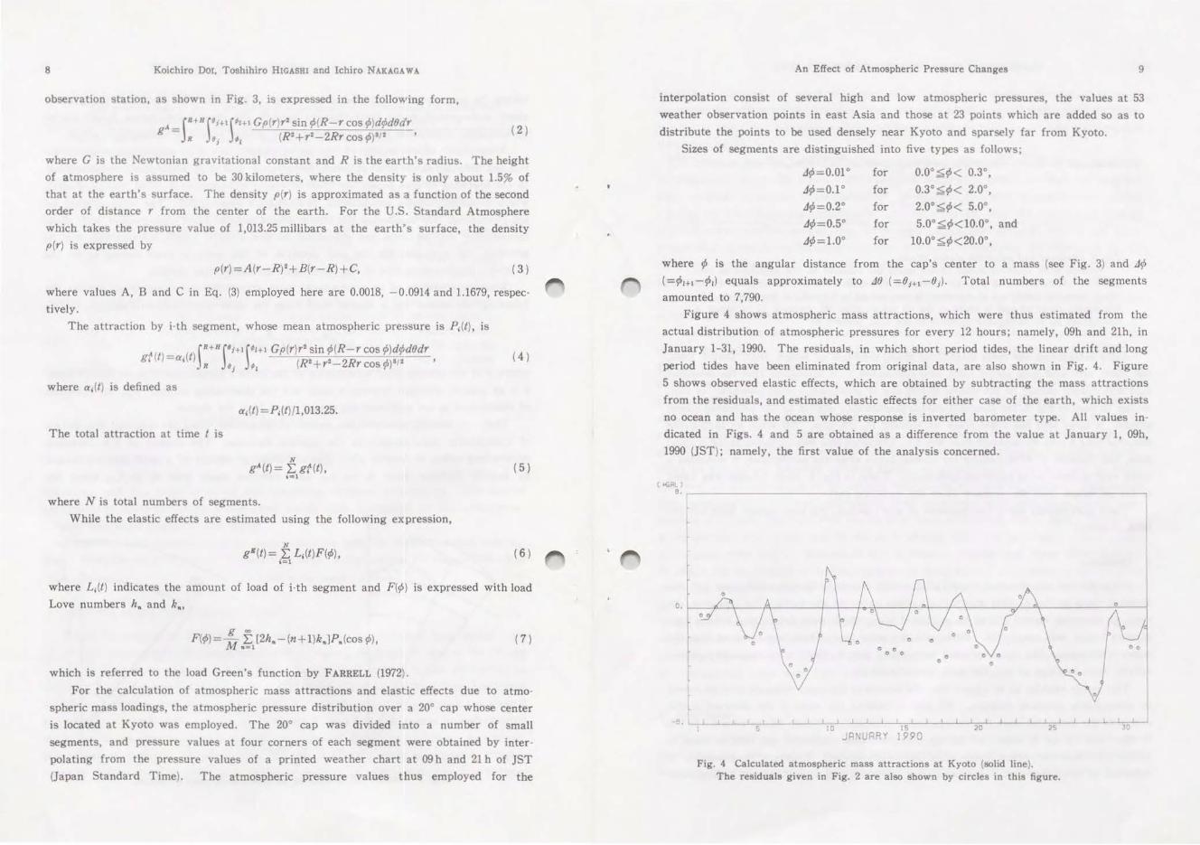
Fig. 5 Observed and estimated elastic effects. Squares show observed elastic effects which are obtained as the difference of two
kinds of values shown in Fig. 4. Thick and thin lines show estimated elastic effects whose response coefficient of the ocean is assumed to be 0.0 and 1.0, respectively. In this figure, about 0.9 pgal is added to the all values after 9h, January 12 to adjust a step caused by an earthquake occurred at 20h 11m, January 11.
After subtracting the mass attractions from residuals in which short period tides,
the linear drift and long period tides were eliminated, it is considered that the remained
part will consist mainly of the elastic effects due to atmospheric mass loadings. In fact,
as can be seen in Fig. 5, the remained part is considerably similar to the estimated elastic
effects. A large step has taken place at January 11, 20h 11m, 1990 when an earthquake
occurred near Kyoto whose magnitude was 5.3. The large step was corrected in the original
data, but, because of data missing for several hours after the earthquake, it remained a
small step without being corrected sufficiently. Then, in Fig. 5, about 0.9 pgal was added
to the all values after 9h, January 12 of the remained part.
There also remain some discrepancies of short period, but their causes have not yet
been identified.
5. Discussion
We compared the observed elastic effects with theoretically estimated ones for two
assumed cases in Fig. 5. One was that no ocean exists on the earth. For this case, the
ratio of observed elastic effects to estimated ones, which were determined by the least
squares fitting, was about 0.74. While, for the other case, which was assumed that the
ocean will respond like as an inverted barometer; that is, there is no response to atmo·
spheric mass loadings at sea, the ratio was about 1.32.
This result enables us to expect that the bottom of the ocean responds to some extent
to atmospheric pressure changes. We also calculated the ratio of the observed elastic
effects to the estimated ones for various ocean response coeftjcient values from 0.0 to 1.0.
If the value of 0.4 is employed for the ocean response coefficient, the ratio is equal to
almost 1.0. However, other causes must also be considered. They are, for examples, an
influence of truncated errors in convolution integrals, and an influence of underground
An Effect o:f Atmospheric Pressure Changes 11
water level changes, for which we neglected in the present study. The effect of some
deviations on the earth's structure from the mean earth's model may appear as a dif·
ference in load Green's functions which can be theoretically calculated by the mean earth's
structural model.
It is not so hard to be free from the influence of truncation errors by the execution
of integration about the whole earth's surface employing global atmospheric pressure
data, although enormous calculations will be needed. But, it is favorable to determine
a range for the integration according to required accuracy. For the rough estimation of
truncation errors in the present case, three assumptions were adopted; that is, the mean
atmospheric pressure on the earth's surface was 1,013.25 millibars, the total load by at·
mospheric pressures was conserve:d and, at everywhere in the range out of 20° cap,
pressures at a certain time were identical. In the data period concerned, a difference
between maximum and minimum of the elastic effects caused by pressure changes of the
outer range was about 0.02 pgal and that of mass attractions was about 0.15 flgal.
It may also be possible to obtain the ocean response and load Green's functions simulta·
neously by applying a linear inve·rsion method using the data of both superconducting
gravity meter and atmospheric pressure distribution. However, more data than, at least,
three times or more what we used 'in the present study are required in order to perform
this inversion. And, the influence of underground water level changes should also be
estimated to perform this inversic:>n accurately excepting the estimation of truncated
errors. Changes in mass attractions due to underground water level changes affect on
gravity as the same direction as those due to atmospheric pressure changes, because,
when an atmospheric pressure becomes higher, an underground water level will be lower,
and then, an attraction due to the underground water will also be smaller. This means
that, after the corrections of atmospheric mass attractions were only made, small com·
ponents of the same direction with atmospheric mass attractions will remain. Therefore,
if the corrections of attractions by the underground water are performed, elastic effects
may appear more clearly. Because of lack to observe underground water level, amounts
of effects due to changes in underground water level can not be estimated, but we infer
that they would be smaller than a half of the elastic effects induced by atmospheric
pressure loadings. We are now investigating a method how to monitor the underground
water level beneath the observation station. It is possible to infer the relative changes
of underground water level by measuring the resistivity of ground for about a day
sampling [HANADA et al. (1990)], but it needs other method to reduce to an absolute value
of underground water level from the resistivity.
6. Conclusion
It was examined the effect of atmospheric pressure changes on gravity changes
employing the data derived from a superconducting gravity meter and atmospheric
pressure distribution within a 20° ocap whose center is located at the observation station.

12 Koichiro Dot, Toshihiro HIGASHI and Ichiro NAKAGAWA
The elastic effects estimated from actual pressure distributions of every 12 hours were
in good agreement with residuals derived by subtracting the earth tides, linear trends
and atmospheric mass attractions from continuous records of gravity changes. However,
there remained some discrepancies of short periods for which causes have not been
identified.
The amount of observed elastic effects was generally greater than that of estimated
elastic effects which were obtained under the assumption that the response is zero on
the ocean. The amount was also less than that estimated under the assumption that no
ocean exists on the earth. There are some possible causes to bring this result. They
are non·zero response of the ocean bottom to atmospheric pressure changes, deviation in
load Green's functions calculated by the mean earth's structural model, influence of under·
ground water level changes and truncation errors of integration. Each of these problems
would be interesting subject for us to be solved.
Acknowledgments
The authors wish to acknowledge Professor S. TAKEMOTO for his helpful discussions
during the course of the present study. The authors wish to thank to Mr. K. FUJIMORI
for his suitable suggestions on how to decrease noises caused by the room temperature
variation. The authors are also indebted to the Kyoto Meteorological Observatory for
offering the printed weather maps.
Numerical calculations in the present study were carried out at the Data Processing
Center of Kyoto University.
References
FARRELL, W.E. (1972): Deformation of the Earth by Surface Loads, Rev. Geophys. Space Phys., 10, 761-797. HAN ADA, H., T. TSUBOKA WA and T. SUZUKI (1990): Seasonal Variations of Ground Water Level and Related
Gravity Changes at Mizusawa, Tech. Rept. Mizusawa Kansoku Center, Nat. Astr. Obs., 2, 83-93. ISHIOURO, M., T. SATO, Y. TAMURA and M. OoE (1984): Tidal Data Analysis-An Introduction to BAYTAP-,
Proc. Inst. Statis. Math., 32, 71 85. NAKAGAWA, I. (1962): Some Problems on Time Change of Gravity. Part 3. On Precise Observation of the Tidal
Variation of Gravity at the Gravity Reference Station, Bull. Disast. Prev. Res. Inst., Kyoto Univ., 57, 2-65. NAKAGAWA, 1., M. SATOMURA, M. 0ZEKI and H. TSUKAMOTO (1975): Tidal Change of Gravity by Means of an
Askania Gravimeter at Kyoto, japan, j. Geod. Soc. Japan, 21, 6 15. NAKAI, S. (1975): On the Characteristics of LaCoste & Romberg Gravimeter G305, Proc. Int. Lat. Obs. Mizusawa,
15, 76-83. OOE, M. and H. HANADA (1982): Physical Simulations of Effects of the Atmospheric Pressure and the Ground
Water upon Gravitational Acceleration and Crustal Deformation, Proc. Int. Lat. Obs. Mizusawa, 21, 6-14. RABBEL, W. and j. ZSCHAU (1985): Static Deformations and Gravity Change at the Earth's Surface due to Atmo
spheric Loading, j. Geophys., 56, 81-99. SPRATT, R.S. (1982): Modelling the Effect of Atmospheric Pressure Variations on Gravity, Geophys. J. R. astr.
Soc., 71, 173- 186. VAN DAM, T.M. and J .M. W AHR (1987): Displacements of the Earth's Surface due to Atmospheric Loading:
Effects on Gravity and Baseline Measurements, J. Geophys. Res., 92, 128I-1286. WARBURTON, R.J. and J.M. GOODKIND (1977): The Influence of Barometric-Pressure Variations on Gravity,
Geophy, J. R. astr. Soc., 48, 281-292.

AN ATTEMPT TO ESTIMATE LOAD GREEN'S FUNCTION FROM GRAVITY CHANGES
INDUCED BY ATMOSPHERIC LOADING
Koichiro DOl
Department of Geophysics, Faculty of Science, Kyoto University

CONTENTS
Abstract - - - - - - - - 1
1. Introduction - - - - 3
2. Data Processing
2.1 Elimination of the Earth Tides, Effect of Polar Motions
and Linear Trend - - - - - - - - - - - - -
2. 2 Estimation of Atmospheric Mass Attraction
------ 7
3. Inverse Problem
3. 1 Formation of Inverse Problem - - - - - - -
3.2 Determination of Number of Model Parameters
3. 3 Solution by Least Squares Method
3. 4 Non-Negative Solution - - - - - - -
4. Comparison between the Obtained Load Green's Function
and Pressure Coefficients
5. Concluding Remarks
Acknowledgements
Appendix A
Appendix B
References
Figure Captions
Figures
Tables
- - - - - - -
- - -
- - -
-
-
-
8
12
14
16
20
23
25
27
28
29
30

Ab stract
In recent years, continuous observations of gravity with
time have been achieved by employing superconducting gravity
meters with long-term stability and high accuracy. As a result,
even small gravity changes associated with atmospheric loading
are now detectable. I t i s, therefore, possible to obt a in
information about the structure of the earth from signals caused
by atmospheric loading.
An attempt to estimate a load Green's function for gravity
was performed using the gravity changes associated with time -
r varying atmospheric pressure loads. Model parameters correspond
ing to discrete load Green's functions were, at first, estimated
by applying the conventional least squares method, but those
absolute values were too large to be acceptable. A similar esti
mation by applying the non-negative least squares method was then
performed. As a result, one parameter obtained for the nearest
region was fairly well consistent with the theoretically predict -
ed one. However, the other parameters could not be determined.
The cause of such a result may be noises included in gravity
changes associated with atmospheric pressure variations.
The only one parameter estimated was almost identical with
the predicted one. On the other hand, absolute values of pressure
coefficients of gravity observed at Kyoto were even smaller than
those predicted for the earth model of a noninverted barometer
type ocean. The smallness of the absolute values of pressure
coefficients should correspond to a large load Green's function
at the neighboring region of the observation site, and it is
1

considered that this discrepancy may also be due to the errors of
observed data. Thus, reduction of noises such as the influence of
underground water and a potent method of inversion are required
for the improvement of the result.
The present method can be employed to estimate ocean
response to atmospheric pressure variations. Furthermore, i t i s
possible to apply the present attempt to a case of oceanic
loading, if the change of sea l evel is accurately determined.
2

1. Introduction
Several load Green's functions for displacement, gravity,
strain and tilt have been theoretically calculated for various
earth structural models during the past three decades. Among
them, those calculated by FARRELL(l972) based on the Gutenberg -
Bullen's earth model are the most famous. Some 1 oad Green's
functions for the earth model with the visco-elastic structure of
the mantle were a 1 s o obtained by ZSCHAU(l978) and
PAGIATAKIS(1990).
The above load Green's functions have been mainly employed
to correct the effects of oceanic and atmospheric loading on
various geodetic and geophysical observations. After the
correction of oceanic loading effects by employing convenient
load Green's functions, observational results such as gravimetric
tides have indicated good agreement with theoretically expected
ones except f o r some o b s e r v a t i o n s i t e s n e a r the
co as t l in e s (MELCHIOR e t a I. 1 9 81, MELCHIOR and DE BECKER 1 9 8 3) .
Th i s me an s t h a t t he e s t i m a t i on o f l o ad G r e en ' s fun c t i on i s
valuable for geodetic and geophysical studies.
On the other hand, there have been few investigations to
estimate the earth's structure from observed signals induced by
some 1 oad i ngs. ZSCHAU (1976) estimated normalized tilt Green's
functions from observed oceanic tidal load tilt. He mentioned
that the indirect effect of oceanic tides in tidal ilt
measurements was capable of providing detailed information on the
crustal and upper mantle structures by comparing the experimental
normalized tilt Green's functions with theoretical ones. However,
3

similar investigations using the indirect effect of oceanic tides
or atmospheric pressure variations in gravity have not yet been
made. One of the reasons for this may be that the stability and
accuracy of gr avimetric observations made
insufficient to detect such loading effects.
s 0 far were
According to PAGIATAKIS(1990), some influence of the visco-
elastic structure of the ithosphere is dominant in the load
Green's function around 0. 5o of angular distance not only in its
phase shift but a I so in amp! i tude change. Therefore, if the I oad
Green's functions are accurately estimated from observations,
some information about inelasticity and the deviation of
structure beneath the observation site from a mean earth model
can be derived. It will also be possible to make more precise
corrections on the effect of oceanic and atmospheric loadings for
the data obtained at each observation site.
Data obtained by superconducting gravity meters at Kyoto
showed clear changes associated with atmospheric pressure
variations, and atmospheric loading effects which were derived
after correction for atmospheric mass attraction were in consid-
erably good agreement with those theoretically predicted(DOI et
al. 1991). It would be an advantage to employ atmospheric pres-
sure data as the load because the data of global atmospher ic
pressure distribution are available at least every twelve hours
and the periods of dominant pressure variations are longer than
those of the principal components of the earth tides. The latter
reason would simplify the procedure to detect the effect of
atmospheric pressure variations from the observed data.
4

We thus tried to obtain the load Green's functions for
gravity employing the data derived from a superconducting gravity
me t e r (mode I TT- 7 0, N 0 0 9) installed at Kyoto as well as from
atmospheric pressure data within 20. oo
was located at Kyoto.
5
cap range whose center

n
2. Data Processing
The data obtained by the superconducting gravity meter
consist of tidal signals as wei as non-periodic changes caused
by the effects of atmospheric pressure and underground water,
contribution from polar motion, instrumental drift,
The observed data can be expressed as follows;
Y a L A j C 0 S (UJ j t + ¢ j
J
+p+D+e
and others.
(1)
where the first term includes the earth tides and the effect of
oceanic tides, and p indicates atmospheric pressure effects in
which underground water level changes caused by atmospheric
pressure variation are involved. D contains the instrumental
drift of the super conducting gravity meter, the effect of polar
motion, crustal movements, seasonal underground water 1 eve 1
changes and those after rainfall. e indicates irregular noises .
In the present study, gravity changes except p and irregular
noises shown in Eq. (1) should be eliminated from the hourly
observed data of the superconducting gravity meter, and then, the
values of 'observed elastic effects' are derived by eliminating
atmospheric mass attraction from the atmospheric pressure effects
p. The data period employed to get 'observed elastic effects' is
about one year and four months from December 1989 to February
19 91.
6

2.1 Eliminations of the Earth Tides, Effect of Polar Motions and
Linear Trend
The tidal analysis program 'BAYTAP-G' (TAMURA et a!. 19 91)
was applied to the data for the removal of the earth tides. After
that, as can be seen in Fig. 1, an almost inear drift is
superposed on the effect of atmospheric pressure. In this figure,
two step-like drifts are also recognized. Their causes are still
not clear, but such irregular drifts usually occurred after some
shock to the gravity meter. In the succeeding data processing,
irregular parts were removed and a least squares fitting was
applied to the remaining data for estimating the inear drift.
Gravity changes are also induced by changes in centrifugal
force caused by polar motion which consists almost entirely of
the annual wobble and the Chandler wobble. Until now, the effect
of polar motion has been detected in the data of superconducting
gravity meters by several researchers (e. g., RICHTER 1985, DE
MEYER and DUCARME 1987).
The amount of gravity changes induced by polar motion can be
theoretically calculated(WAHR, 1 9 8 5) According to the
calculation, gravity changes amounting to nearly 10 f.1. gals are
expected at Kyoto from the IRIS data.
Drifts in which any linear trend has been removed and the
expected effects of the polar motion are shown in Figure 2. In
the calculation, we assumed that gravimetric factor o was 1.16
and phase shift was zero. In this figure, the later part of the
drifts is in good agreement with the expected effects of the
polar motions, but these effects were not found clearly in the
7

early part due to the step-like gravity changes.
Because of the shortness of the present data period and the
disturbances in the early part of the drifts, the determination
of amplitude and phase of the polar motion is difficult.
Therefore, interpolated values of the expected effects shown in
Fig. 2 were removed from the drifts in order to correct the
effects of polar motion.
Fig. 3 shows atmospheric pressure variations and gravity
changes associated with pressure variations during the present
data period.
2. 2 Estimation of Atmospheric Mass Attraction
Gravity changes associated with atmospheric pressure varia
tions can be divided into two parts. That is,
p pA + pE, (2)
where pA is the Newtonian attraction by atmospheric mass and pE
is the elastic effect induced by atmospheric pressure loadings.
Atmospheric mass attraction pA can be estimated from the data of
atmospheric pressure distribution around Kyoto.
Data of atmospheric pressure distributions are required to
calculate the atmospheric mass attraction. In the present study,
we have used printed weather charts or radio weather broadcasting
to get pressure data at several tenth points in east Asia, Japan
and the north-western Pacific. Many co-circle data whose center
was located at Kyoto have been generated from the data of several
8

tenth points by interpolating. The outermost circle was placed at
20. o· angular distance from Kyoto.
The attraction of an atmospheric mass at any giventime was
calculated as the summation of the attractions of small seg-
ments. One of them is shown in Fig. 4(a). The attraction of a
small segment is calculated using the following expression:
I R+H fa J•lf ¢lot pA = a,(t) ...
R a, ... 1
G p (r)r 2 sin ¢ (R-rcos ¢ )d ¢ d 8 dr
(R 2 + r 2 -2Rrcos¢) 3 / 2
r where al (t) is defined with surface pressure PI (t) as
a1 (t) • Pt (t) I 1013. 25,
( 3)
(4)
and p ( r) is atmospheric mass density distribution in the
direction of radius which was derived by approximating that of
the U.S. Standard Atmosphere with a quadratic function as
P(r) = A (r-R) 2 + B (r-R) + C, ( 5)
where values A, B and C employed here are 0. 0018, -0.0914 and
1.1679, respectively . G is the Newtonian gravitational constant
and H is the height of the atmosphere. R is the radius of the
earth, r is the distance between the center of the mass and the
earth's center and ¢is the angular distance bet7<een the
observation site and the center of the atmospheric oass(DOI et
al. 1991).
9

Calculations of atmospheric mass attraction were performed
for 531 atmospheric pressure distribution data from December
, 1989 to February, 1991. Finally, the 531 calculated attractions
were removed from the corresponding gravity changes associated
with atmospheric pressure variations, and the residual pEs were
then obtained. Those are considered to be the values of 'observed
elastic effects'.
Before estimating the load Green's function for gravity, it
should be noted that the values of 'observed elastic effects' are
not net values which only consist of atmospheric loading effects,
but those contain unknown offsets of the superconducting gravity
meter. Therefore, deviations from the initial value, namely,
pE(i) - pE(l), were employed as the observed values and they are
hereinafter referred to as 'observed elastic effects'. A similar
procedure was also applied at the making of the loading matrix
L.
The 'observed elastic effects' and predicted ones calculated
with Farrell's load Green's function for gravity are shown in
Fig. 5 together with atmospheric pressure variations at Kyoto
during the period from December 1, 1989 to February 28, 1991.
Since we used the data of atmospheric pressure distribution
within only a 20. oo range from the observation station, the
effect of the outer region, namely, a truncation error, may be a
cause for the error of the solution. To estimate the truncation
error roughly, three assumptions were adopted. The first is that
the mean atmospheric pressure on the earth's surface is 1013.25
millibars, the second is that the total load by atmospheric
1 0

pressure on the earth is conserved, and the last is that atmos-
pheric pressure anywhere in the outer region at a given time is
identical. The amount of truncation error at each time was esti
mated with the same method as applied for the inner region and .
the maximum value of mass attraction was about 0. 2 p. gal. While,
that of elastic effects was about 0. 02 fl. gal. These corresponding
values were removed from the observed values.
1 1

3. Inverse Problem
3.1 Formation of Inverse Problem
The load Green's function for gravity is represented as
co I I
F(¢) = g/MI:[2hn- {n+l) knJPn (cos¢), ( 6)
n=l
where h:, and k~ are the load Love's number (FARRELL 1972). Using
this Green's function, elastic effects induced by a load at a
time t can be theoretically calculated, that is,
M
pE (7)
L(¢j) is a load applied at a distance of ¢j from the observation
station. To estimate a load Green's function from observational
results, the right side of Eq. (7) is equated with the 'observed
elastic effects' pE{t 1 ), that is,
M
(8)
j = 1
Eq. (8) is simply expressed as follows:
12

~ ~
pE • LF, (9)
~ ~
where pE is the vector (pE(td, ... ,pE(tm))-r, F is the vector (F(
,FC¢n)-r and L is the load matrix, whose elementL(i, j) at
the distance ¢J at the time t 1 is
(1 0)
and T deno tes transposition.
~
The discrete load Green's function vector F can be obtained
by solving a problem the inverse of Eq. (9), namely
( 1 1)
where W is the weight matrix, and the superscript -1 denotes the
inverse condition.
Although we tried at present to solve only the simplest case
in which the elastic earth with no ocean was assumed, i t i s
possible to form more complicated observational equations instead
of Eq. (8). When the response of the ocean to atmospheric pressu re
is taken into consideration, the observational equation is
expressed by
M
pE ( t d (12)
13

where superscripts c and o indicate the continent and ocean,
r esp e c t iv e ly . T hen th e coefficient ma t r i x is
L ~
-+ and the vector F to be solved is
From the 'observed load Green's function' F, ocean respons e 'Y at
the distance ¢J is found by
(13)
The estimation of ocean response 'Y(</>J) will provide sig n ificant
information about interactions among the solid earth, ocean and
atmosphere.
3. 2 De t ermination of the Number of Model Parameters
Although a load Green's function in itself is a continuous
function, we can only derive the function in the discrete form
because of the limitation of observed data.
Since it was projected that Eq. (11) would be difficult to
14

solve having many parameters and an interesting feature in the
load Green's function at a range less than about 2. 0° for a more
r e a 1 i s t i c v i s c o- e 1 a s t i c e a r t h m o d e 1 ( P A G I AT AK I S 1 9 9 0) , we m a i n 1 y
investigated the load Green's function at a range within 2. 0°.
The elements L(i, j) ja1,n) of the applied load
matrix L consist of the loads of small segments which are dis-
tributed within the distance from ¢J to ¢J-1• ¢J indicating one
boundary of a sect i on .¢1 - 0. 0 o and
of j-th section at the time t 1 is
c/Jn-1 - 2. oo. Then the 1 oad
KJ Lx
L (i, j} [; S(k,l)P(i,k,l)/980.25.
where P(i,k, 1) is the mean pressure of a segment and S(k,l) is
the area of the segment (see Fig. 4 (b)). KJ is the number of co
circles in the j-th section and Lx is the number of segments in
the k-th co-circle of the j-th section. The number n is the
number of sections, and the number m equals that of observations
made , that is to say the number of the 'observed elastic
effects'. The boundary cpJ was determined so as to make the area
of each section almost identical.
Next, it was necessary to decide the number of model parame
ters to be solved within 2. 0°. To determine the number of parame
ters, we have examined the model resolution matrix. It indicates
whether the parameters can be independently predicted, or r e-
solved. If the resolution matrix is equal to the identity matrix,
1 5

that is, diagonal elements are one and other elements are zero,
then the parameters can be sufficiently resolved. If it is not
the identity matrix, then the estimated parameters are weighted
averages of the unknown 'true parameters'. The model resolution
matrix is defined as R L-~L. where L-~ indicates the general-
ized inverse of L(MENKE 1989).
For various cases of the number of parameters, the model
resolution matrices were investigated. As a result, the
resolution matrix was far from the identity matrix when the
number of parameters was greater than six. Therefore, we set the
number of model parameters at five. The model resolution matrix
for five parameters is shown in Table I. Although this resolution
matrix is inconsistent with the identity matrix in the strict
sense, it will not induce serious problems in the results of the
present study.
3. 3 Solution by Least Squares Method
To solve the inverse problem according to Eq. (11), a weight
matrix for observed data is required. The weight matrix W, whose
elements were W(i, j) (ic1,m, j~1,m), was estimated by a
Biweight-method (e. g., NAKAGAWA and OYANAGI 1982). The de t a i 1 e d
operations to make the weight matrix are shown in Appendix A.
The results obtained for the case of five unknown parameters
are shown in Table II. The first column indicates the boundaries of
a range corresponding to each parameter, and the second column is
the load Green's function obtained from the 'observed elastic
effects'. Predicted parameters are also shown in the third column
1 6
of this table to compare them with the observed ones. The j-th
theoretical value g 0 (j) was calculated from Farrell's load
Green's function G(¢) by the following expression,
g 0 ( j) (14)
where NJ (¢J- ¢J-1)/D,c/J. The last column indicates the parame-
ters solved using theoretical elastic effects instead of the
observed ones.
The parameters derived from observed data are so large when
compared with the predicted ones shown in the third column that
those are not acceptable. However, because the parameters ob-
tained from theoretically calculated data in the fourth column
are almost the same as the predicted ones, the discrepancies
between the second and third columns might be caused by errors in
the observed data.
The influence of underground water level changes after
rainfall or those of seasonal changes may, especially, cause
cons ide r a b l e o b s e r vat i on a l no i s e s. I t i s however, difficult to
estimate the influence without information about hydrology around
observation station. Since there are no available data about
underground water level, we can only estimate possible gravity
changes for a simple model. We assumed a disk of aquifer with
radius R placed at the depth D. Then, gravity change induced by
the disk is given by
17

where d is thickness of the disk, pis density of water and T) is
porosity. If D•lO meters, d•l centimeter, R•l kilometer and
TJ .. 0. 1 are assumed, [lg is about 0. 042 f1- gal. This means that
twenty or thirty centimeters change in underground water level
can induce about one fi-gal gravity change. This will become a
considerable large noise.
As described above, the 'observed elastic effects' contain
various noises such as the influence of underground water To
examine those or observational errors to the solution, i t i s
convenient to use a condition indicator ~(A) of matrix A shown in
the following equation,
~ ~
y • Ax.
The de f i n i t i on o f t he con d i t i on i n d i c a t or JC (A) is given in
Appendix B. As can be seen from Eq. (B-2), relative errors in the
~ ~
observed data vector y may appear in the solution vector x
amplified by JC(A) times. In this case, thecondition indicator
/C(L) of load matrix L is about 5. OX10 4• This fact means that the
solution of observational equation (9) is very sensitive to
o b s e r v a t i on a I e r r or s and not r e I i a b I e (HI TOTS UMA TU 1 9 8 2) .
To examine the characteristics of JC(L) in the present data
kernel matrix L, some trial-and-error numerical experiments were
carried out, and three rough tendencies were derived. The first
one is that JC(L) becomes larger according to the increment of
1 8
number of parameters to be solved. The second one is that, if the
number of parameters is constant, JC(L) takes a smaller value when
the number of elements of a certain row are almost the same
order. The third one is that it takes a smaller value in direct
proportion to the number of observed data. The first character
means that the higher is the resolution, the more unstable are the
solutions. It is found from the second character that a manipula- .
tion which equalizes the area in which atmospheric loads are
applied is effective to stabilize the solution. But this manipu
lation brings about lower resolution near the observation station
and higher resolution far from it. For all these defects of the
manipulation, we were able to employ it to form the matrix L.
1 9
3.4 Non-Negative Solution
As can be seen in Tableii, the absolute values of solutions
derived by the least squares method were too large, and contained
several negative values. The cause of this result is, as men-
tioned in preceding section, that the observational equation is
sensitive to observational errors. Hence applying some con-
straints will make the condition of equation improve. The parame-
ters within 2.0• should be positive, when we take the direction
of gravity as positive. There was a lso an example of seismic
inversion wherein the parameters obtained by the non-negative
least squares method were considerably improved(WIDMER et al.
1991). So that,wesolved Eq. (9) again under the constraint that
all of the parameters FJ(jc1,n) were non-negative, that is,
~ ~
minimizing II LF - pE II subject to FJ ~ 0.
The non-negative least squares method is a particular case
of the least squares method with linear inequality constraints,
~ ~b II ~ ~ namely, minimizing IIAx - subject to Cx~d. Since the
mathemat ical background, details of the algorithm to solve the
inverse problems under the inequality constraints and the FORTRAN
program for that purpose are described in some textbooks (e. g.,
LAWSON and HANSON 1974, MENKE 1989), we omit them here.
Results obtained by using the non-negative least squares
method are shown in Table ill, and also in Fig. 6 by dotted area.
In Fig . 6, the load Green's function by FARRELL(1972) and the
averaged one derived from Farrell's are also shown by solid I ioe
and shaded area, respectively. The results are much improved over
those in Table II which correspond to ordinary least squares
20

solutions. The result at the range from 0. o· to 0. 89° is only
slightly smaller than the predicted value, which is shown in the
third column of Table III. The other results shown in the second
column of Table III are all zero. The last column indicates the
parameters derived from theoretically calculated elastic effects
instead of the observed ones.
In the algorithm of the non-negative least squares method,
the initial values of unknown parameters are assumed to be zero
at the first stage to compute the gradient vector of total error.
~
Here, the total error is defined as e(F)
~ ~ ~ A
-> II LF
~
pE 11 2 I 2 and the
~
grad i en t v e c t or i s L (LF pE) at F F. And then, each of the
parameters is improved from the initial value by conventional
least squares methods, f the corresponding component of the
negative gradient vector is positive. Therefore, if all compo-
nents of the negative gradient vector become negative at the
state where some of the parameters are improved from zero, the
other parameters remain zero. This fact may suggest that the
parameters when equal to zero can't be determined.
Since a similar ana ly sis executed for the theoretical data
set of elastic effects containing no noises showed almost equal
values to the predictedparameters, the results shown in Tableiii
may be caused by noises included in the observed data. To examine
the influence of observational errors, noises with various
amplitudes determined by eX(-1) t were artificially applied to the
theoretical data set, where e is an amp! itude of noise, and then
the solutions for the data with various noises were obtained by
applying the non-negative least squares method. The results of
21

the numerical experiments are shown in TableN. This indicates
that the errors of observed data must be reduced under the level
of 10- 5 #gal to obtain parameters significant to two figures. I t
is considered that this noise level corresponds to the value of
the condition indicator .t(L).
22

4. Comparison between the Obtained Load Green's Function and
Pressure Coefficients
As the extent of the responses of gravity to atmospheric
pressure variations can be evaluated by calculating the Newtonian
mass attraction and the effect of atmospheric pressure loading, a
theoretical response coefficient can be obtained by adding the
two effects. Thus, t is possible to justify to some extent
whether the estimated load Green's function is reasonable or not
by comparing the observed pressure coefficients with the theoret
ical response ones. Theoretical response coefficients at Mizusawa
have already estimated by SATO et al. (1990) using global baromet-
ric pressure distribution. According to them, they were -0. 387
and -0. 296(,ugal/mb) which were calculated for the ocean of types
both the inverted and the non-inverted baromete r, respectively.
They also mentioned that the pressure coefficient at Mizusawa by
a superconducting gravity meter was -0.386 (,ugal/mb).
Observed response coefficients which were obtained from the
monthly data at Kyoto during the period from December 1989 to
February 1991 are shown in Fig. 7 with two theoretically calcu-
lated values at Mizusawa by dashed in e s. The the ore t i c a I r e-
sponse coefficients at Kyoto wi II, of course, be different from
these two values at Mizusawa, but their differences must be small
because the distribution of land and ocean around Kyoto doesn't
differ much from that around )fizusawa. Thus, we may employ these
values as criteria.
Absolute values of all the observed responsecoefficients
are less than the theoretical value -0.387(,ugal/mb) for the ocean
23

of the inverte d barometer type, and some of them are even smal Jer
than that for the non-inverted barometer case(-0.296(,LLgal/mb)).
In the effect of atmospheric pressure, the Newtonian attraction
is the major component, and the elastic acceleration induced by
atmospheric loading acts in the opposite direction to the Newto
nian attraction. The small absolute values of response coeffi
cients are considered to correspond to the large elastic effect.
As the effect of loads at the neighborhood of the observation
station is more significant, t is considered that the small
pressure coefficients correspond to the large load Green's func
tion at the neighborhood region.
The observation site at Kyoto University is not fixed on bed
rock but on sediment. Large responses of the ground to
atmospheric pressure loadings are therefore expected around the
observation site, and the response coefficient of gravity will
then take a smaller absolute value than the theoretically pre
dicted one.
On the other hand, the result of the observed I oad Green's
function of the nearest region in Fig. 6 or Tab I e ill showed an
almost identical value with the predicted one, so it appears to
be incompatible with low pressure coefficients. Although ts
cause is not clear, as can be seen in TableN, noise contamina
tion may induce the incompatibility.
24

5. Concluding Rem a rks
An attempt to obtain the load Green's function by employing
the observational data of a superconducting gravity meter at
Kyoto was performed. Because of the unreliability of the coeffi -
cient matrix and contaminating observational noises, acceptable
model parameters could not be estimated by the ordinary l east
squares method. The parameters were then estimated by applying
the non-negative least squares method. One parameter derived for
the nearest region from the observation station showed a rela
tively reasonable value while others have not yet been deter
mined. Only one estimated parameter was almost identical with the
theoretically expected value. However this fact is inconsistent
with the smallness of absolute values of pressure coefficients at
Kyoto.
Consequently, in order to estimate the load Green's function
from observed data, it is essential to reduce observational
noises. The major source of observational noise to be considered
would be underground water level changes. They can be divided
into two components; one is associated with atmospheric pressure
variat i ons and the other are the temporal changes after rainfall
or seasonal changes. As the latter component is often fairly
large, gravity changes induced by these changes seriously inter
fere with the determination of load Green's function. For this
reason, it is very impo r tant to monitor underground
to obtain more reliab l e so l utions.
water levels
In the present study, we assumed that densities at any
atmospheric height were proportional to the earth's surface
25
pressure. The act u a 1 atmosphere, however, is more complicated
than assumed. Perturbations from the atmospheric model which we
employed in the present study would cause those of Newtonian
attraction, and they would remain in the 'observed elastic
effect' values as observational noise. If the data of atmospheric
density distribution in the direction of height were available,
the 'observed elastic effects' could be almost free from noise of
this kind.
As shown in TableN, it is desirable to reduce noise to the
level of 10- 15 ,agal in order to accurately estimate the load
Green's function. However, in practice, it is impossible to do
so. Therefore, we should search for other methods to select model
parameters in order to improve the condition indicator
more potent methods to estimate the parameters.
/C(L) or
Although the attempt to obtain the load Green's function
observationally was not successful in the present study, an
investigation of this kind should be continued to clarify the
heterogeneities of structures and visco-elastic characteristics
within the earth. Another purpose is the correction of geodetic
and geophysical data with very high accuracy.
In the present study, we employed atmospheric pressure
loading as the input signal to the earth. It will be possible to
make a similar attempt with load changes being effected by sea
level changes, if they are accurately determined. By using two
types of these loads changes, a more detailed load Green's func
tion may be determined.
26

Acknowledgements
The author wishes to thank Professor Ichiro NAKAGAWA for his
hearty encouragement and helpful discussions during the course of
the present study. The author is also grateful to Professor Shuzo
TAKEMOTO for his helpful discussions and pertinent advice. The
author is indebted to Mr. Toshihiro HIGASHI for his diligent
maintenance of the continuous observations by two superconducting
gravity meters and the arrangement of their data. The author
wishes also to thank to th e National Astronomical Observatory of
Mizusawa, Japan for offering the IRIS data. The author is also
grateful to Professors Torao TANAKA, Norihiko SUMITOMO, Tamotsu
FURUSAWA and Kazuo OIKE for their critical reading of the manu
script. The author wishes to thank Dr. Yutaka TANAKA, Dr. Kunio
FUJIMORI and the members of the laboratory of Kyoto University
for their valuable discussions.
Numerical calculations in the present study were carried out
at the Data Processing Center of Kyoto University.
27

Appendix A
Diagonal components w(i) of W are calculated according to
the following expression,
1- (z(i)/sc) 2 <lz(i)l <sc)
w ( i)
0. 0 ( \z(i)l > sc ), (A- 1)
wh e r e z ( i ) i s t he no r m a I i z e d r e s i d u a I and i t i s de f i ned a s
follows;
z (i) = v (i) Ia. (A-2)
s median( lz(i)l ),
wh e r e v ( i ) i s t he de v i a t i on f r om the t he o r e t i c a I v a 1 u e. a i s
r. m. s. e. of observed values and c is the scale factor. Components
except diagonals are zero.
28

Appendix B
The condition indicator JC(A) is defined as follows:
= IJ.max/fi.min, (B -1)
where, IIAII means the norm of matrix A, and fl.max and IJ.min indicate
the maximum and minimum of the singular value of matrix A,
respectively. Using JC(A), the relative error of solution vector~
is estimated from the following expression,
(B- 2)
~
where oY is ~
the error vector of observation vector y(NAKAGAWA and
OYANAGI 1982). This expression indicates that, if JC(A) is large,
there is the possibility of a gross error through observational
errors, with such cases often being called a 'sensitive
problem' (e. g. HITOTSUMATU 1982).
29

REFERENCES
DE MEYER, F. and B. DUCARME (1987): Long Term Periodical Gravi-
ty Changes Observed with a Superconduct ing Gravimeter, Bul I.
Inform., Marees Terr., 99, 6902 - 6904.
DO I , K. , T. H I GASH I and I . NAKAGAWA ( 1 9 9 1 ) : An E f f e c t o f
Atmospheric Pressure Changes on the Time Change of Gravity
Observed by a Super conducting Gravity Meter, J. Geod. Soc. Japan,
37, 1 - 12.
FARRELL, W. E. (1972): Deformation of the Earth by Surface Loads,
Rev. Geophys. Space Phys., 10, 761 - 797.
HITOTSUMATU, S. (1982) Numerical Analysis, Asakura-Shoten,
Tokyo, 163 p.
LAWSON, C. L., and D. J. HANSON (1974): Solving Least Squares
Problems, Prentice - Hall, Englewood Cliffs, New Jersey, 340 p.
MELCHIOR, P. , M. MOENS, B. DUCARME and M. VAN RUYMBEKE (1981) :
Tidal Loading along Profile Europe - East Africa - South Asia -
Australia and Pacific Ocean, Phys. Earth Planet. Inter., 25, 71-
106.
30

MELCHIOR, P. and M. DE BECKER (1 9 8 3) A Discussion of World-wide
Measurements of Tidal Gravity with Respect to Oceanic Interac
tions, Lithosphere Heterogeneities, Earth's Flattening and Iner
tial Forces, Phys. Earth Planet. Inter., 31, 27- 53.
MENKE, W. (1989): Geophysical Data Analysis: Discrete Inverse
Theory, International Geophysics Series, Vol. 45, Academic Press,
Inc., San Diego, 289 p.
NAKAGAWA, T. and Y. OYANAGI (1982): Experimental Data Analysis by
Least Squares Method, University of Tokyo Press, Tokyo, 206 p.
PAGIATAKIS, S. D. (1990): The Response of a Realistic Earth to
Ocean Tide Loading, Geophys. J. Int., 103, 541 - 560.
RICHTER , B . (1985): Three Years of Registration with the
Superconducting Gravimeter, Bull. Inform. , Marees Terr., 94, 6344
- 6352.
SATO, T., Y. TAMURA, N. KIKUCHI and I. NAITO (1990): Atmospheric
Pressure Changes and Gravity Changes, and the Applications to
Geophysics, Proc. Workshop 'Searching of the Earth with Nano-Gal
Level Observation', Mizusawa, 27- 31.
TAMURA, Y. T. SATO, M. OOE and M. ISHIGURO (1991): A Procedure
for Tidal Analys i s with a Bayesian Information Criterion, Geo
phys. J. Int., 104, 507 - 516.
31

WAHR, J. M.
Geophys. Res.
(1985): Deformation Induced by Polar Motion, J.
90, 9363 - 9368.
WIDMER, R., G. MASTERS and F. GILBERT (1991): Spherically
Symmetric Attenuation within the Earth from Normal Mode Data,
Geophys. J. Int., 104, 541 - 553.
ZSCHAU, J. (1976): Tidal Sea Load Tilt of the Crust, and Its
Application to the Study of Crustal and Upper Mantle Structure,
Geophys. J. R. astr. Soc., 44, 577 - 593.
ZSCHAU, J. (1978): Tidal Friction in the Solid Earth: Loading
Tides versus Body Tides, in Tidal Friction and the Earth's
Rotation, eds. BROSCHE, P. and J. SUNDERMANN, Springer-Verlag ,
Ber l in, 62- 94 .
32

Figure Captions
Fig. 1 Trends whic h were derived after the removal of the earth
tides from the original data. The data period is from December
1989 to February 1991. One division of the abscissa is 10 days.
Unit of figures of the ordinate is ,££gal. Non - linear drifts are
indicated by arrows.
Fig. 2 Expected effects of polar motion on gravity and trend
which was derived after the removal of the earth tides and a
linear trend from the original data. The data period is the same
as that in Fig. 1. One division of abscissa is 10 days and that
of ordinate is 1 ,££gal. Effects of polar motions are indicated by
circles and solid lines indicate the trend.
Fig. 3 Atmospheric pressure variation(upper) and gravity changes
associated with pressure variation(lower). One division of the
ordinate corresponds to 30 mb for atmospheric pressure variations
and to 15 .agals for gravity changes. One division of the abscissa
is one day.
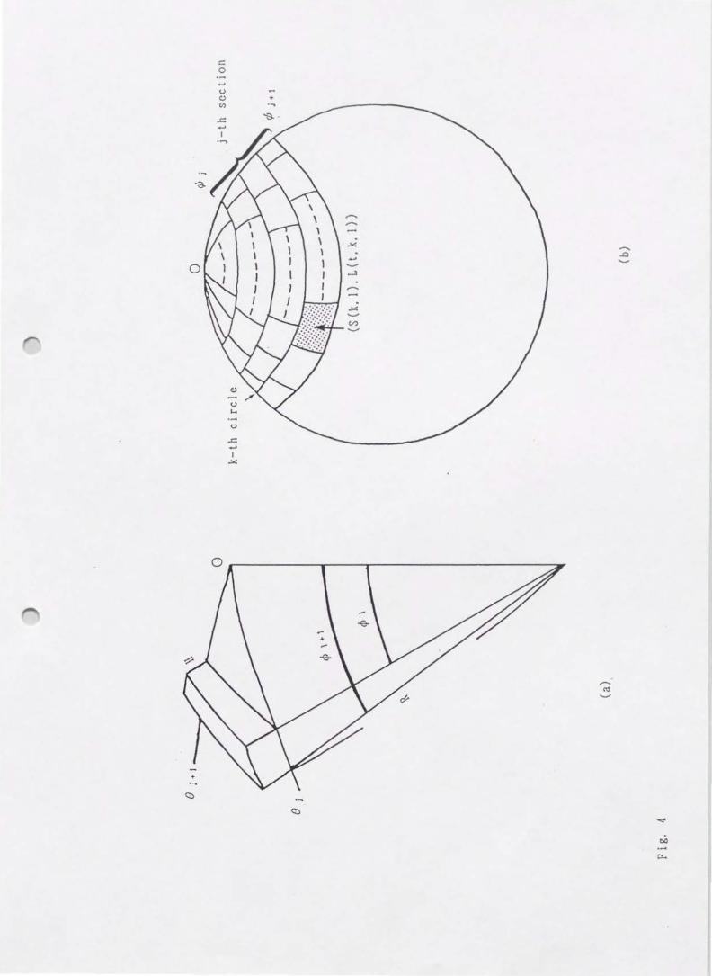
Fig. 4 a) Notations to calculate atmospheric mass attraction.
An atmospheric mass is surrounded by angular distance from¢ 1
to¢ 1+1 and azimuth from e to B HI. H is height of atmosphere and
R is radius of the earth. 0 is observation station.
b) Notations to calculate atmospheric pressure loading.
S(k, 1) indicates the area of dotted segment and L(t, k, I) is the
load imposed on the segment.
33

Fig. 5 Derived 'observed elastic effects'{+) and theoretical
e 1 a s t i c e f f e c t s (Q) w i t h a t m o s ph e r i c p r e s sur e v a r i a t i on (so 1 i d
line). One division of the ordinate corresponds to 30 mb for
atmospheric pressure variation and to 4 ~gals for gravity
changes. One division of the abscissa is one day.
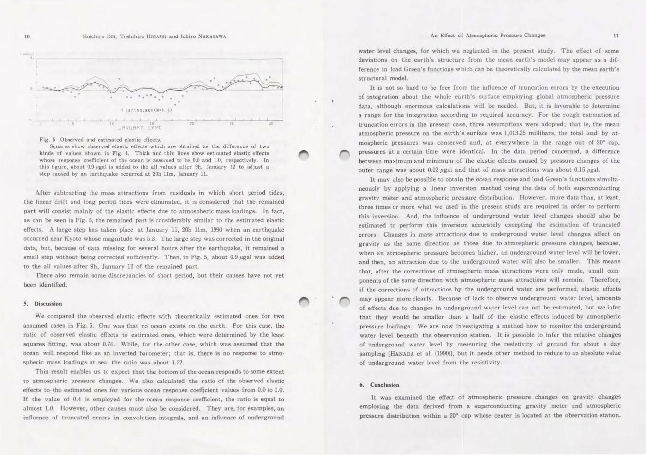
Fig. 6 Load Green's function for gravity estimated by non-
negative least squares method. The estimated load Green's
function is shown by the dotted area and the averaged one
obtained from Farrell's is shown by the shaded area. A solid line
indicates Farrell's load Green's function for Gutenberg's earth
mode 1.
Fig. 7 Observed response coefficients of gravity to atmospheric
pressure variations obtained from monthly data to Kyoto. The data
periodis the same as that in Fig. 1. The upper dashed ine
indicates a predicted response coefficient for the earth which
has the ocean of the inverted barometer type. The lower one
indicates that for the earth which has the ocean of the non
inverted barometer type.
Table I Model resolution matrix for five parameters
34

Table 1I Estimated load Green's function for gravity by the least
squares method
Corresponding ranges to five parameters are shown in the
first column. The estimated load Green's function from 'observed
elastic effects' and the predicted one are shown in the second
and third columns, respectively. In the last column, the
estimated load Green's function from the theoretical elastic
effects is indicated.
Table ill Estimated load Green's function for gravity by the non
negative least squares method
Corresponding ranges to the five parameters are shown in the
first column. The estimated load Green's function from 'observed
elastic effects' and the predicted one are shown in the second
and third columns, respectively . In the last column, the
estimated load Green's function from the theoretical elastic
effects is indicated.
TableiV Influences of given noises with various amplitudes
Amplitudes of given noises are shown in the first column.
Corresponding ranges to five parameters are indicated in the top
row.
35

0
N N
......

E) E)
~ E) E) E)
~ E) E) E)

0 ...J X: a:
c.:> 0 ~ c.!) 0 ,....,
U1 >a: 0
0
('?
t>O
c.:...
:::: 0
I .X
.........
.........
-.X
,_.)
.X
V) .._,
-.0 .........

+ 0 + 0 +0 + 0 + 0 + 0 .p-+ 0 + 0 (f) + 0
~~ ~ >-+ 0 + 0
+.t ~ a: + 0 + 0 0 + 0 f ~ J ~ + 0 -£) + 0 + 0 ~ + 0 0 + 0 + 0 + 0 + 0 + 0 l ~ + 0 + 0 + 0
* 8 ~ ! ~ + 0 + 0
* ~ 01' ~ + 0
+ 0 t 8 + 0 + 0 + 0 + 0 + 0 + 0 +0 +0 + 0
+ 0 :t@ +0 ~ 8 + 0 +0 + 0 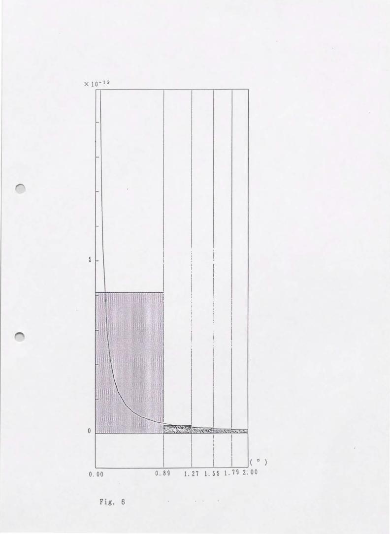
~-------------L-----L----~--~~ ( 0 )
0. 00 0. 8 9 1.27 1.55 1.19 2.00
Fig. 6

( J1. ga 1/mb) -0.4.-----------~~------------------------------------------.
~ ~
-0. 3 - - - - - - - - - - - - - - - - - - - - - - - - - - - - E!)- - - - - - - - - - - - - - - - - - - - -~
-0. 2 f-
-0. 1 I I I I I I I I I
DEC JAN FEB HAR APR HAY JUN JUL AUG SEP OCT NOV DEC JAN FEB
Fig. 7

Table I
1 2 3 4 5 1 1. 009 0. 011 0. 007 0. 012 0. 00 9 2 0. 0 11 1. 013 0. 0 09 0. 015 0. 0 11 3 0. 0 01 0. 009 1. 0 06 0. 010 0. 0 07 4 0. 012 0. 015 0. 010 1. 017 0. 012 5 0.009 0. 011 0. 007 0. 012 1. 0 0 9
Tabl e II
Range Est i rna t ed Pr ed i c t ed Pa r ameter from (unit : deg ree) Paramete r Parame t er Theoretical Value
0. 00 - 0. 89 -4. 0 5 X 1 0- I I 4. 10 X 10-13 4. 10 X 1 o- I 3
0. 8 9 - 1. 2 7 1. 7 8 X 1o-le 2. 38 X 10- 14 2. 38 X 1 o- I 4
1. 27 - 1. 55 -4. 6 8 X 1 o- 10 1. 6 3 X 10- 14 1. 6 3 X 1 o- I 4
1. 55 - 1. 7 9 1. 9 8 X 10 - 10 1. 27 X 10 - 14 1. 2 7 X 10- I 4
1. 7 9 - 2. 0 0 -7. 6 3 X 1 0- I I 1. 0 5 X 10 - 14 1. 0 5 X 10 - I 4

Table m
Range Est i rna ted Predicted Parameter from (unit: degree} Parameter Parameter Theoretical Value
0.00 - 0.89 4.08 X 10⁻¹³ 4. 10 X 10-13 4. 10 X 1 o-, 3
0.89 - 1. 2 7 0. 0 2. 38 X 10- 1 4 2. 38 X 10- 1 4
1. 2 7 - 1. 55 0. 0 l. 6 3 X 10- 1 4 1. 6 4 X 1 0- 1 4
1. 55 - l. 7 9 0. 0 l. 2 7 X 10 -1 4 l. 2 7 X 10- 1 4
l. 7 9 - 2. 00 0. 0 l. 0 5 X 10-14 l. 0 5 X 10- \ 4
Table IV
Range 0. 00 - 0. 89 0.89- 1. 2 7 l. 2 7 - l. 55 l. 55 - l. 7 9 l. 7 9 - 2. 00 (degree} Noise
(JJ. gal}
1.0 2.o2x1o- 13 2. 52 X 10- 13 0. 0 0. 0 0. 0
lo-t 3.52xlo- 13 1.11X10-I 3 0. 0 0. 0 0.0
10 - 2 4.11Xl0- 13 0. 0 7. 76X 10- 14 6. 37x lo-ts 0.0
10- 3 4.13xlo- 13 7. 78x lo-ts 5. 46 X 10- 14 1. 89X 10- 16 1.33X10- 14
10- 4 4.10Xl0- 13 2. 22X 10- 14 2.01Xl0- 14 l.l4Xl0- 14 1. 07X 10 - 14
lo-s 4.10Xl0- 13 2. 37X 10- 14 1. 67X 10- 14 1.26Xl0- 14 l.OSXl0- 14
0. 0 4.10X10- 13 2. 38X 10- 14 1. 63X 10- 14 1.27X10- 14 1. 05X 10- 14