Travel times in complex environments

Adrien DAGALLIER(1,2), Sylvain CHEINET(1), Daniel JUVE(2), Aurélien PONTE(3), Jonathan GULA(3)

(1)Institut de recherche franco-allemand de Saint-Louis, Saint-Louis 68300, France, adrien.dagallier@isl.eu(2)Université de Lyon, Ecole Centrale de Lyon, Laboratoire de Mécanique des Fluides et d’Acoustique, Unité Mixte de

Recherche, Centre National de la Recherche Scientifique 5509, Ecully F-69134, France(3)Université de Brest, CNRS, IRD, Ifremer, Laboratoire d’Océanographie Physique et Spatiale (LOPS), IUEM, Brest 29280,

France

AbstractTimes of Arrival (TOAs) of propagated signals are of utmost interest in seismic, underwater as well as aerialacoustics. From TOAs, one may reconstruct the propagation media properties from known sources and sensorspositions, or conversely, find sound events locations in a known environment. Modeling the TOAs in realisticenvironments (wind or current, sound speed gradients, obstacles. . . ) requires a general physical model, ableto factor in the impact of refractive and diffractive processes. We present an interface-tracking model basedon Sethian’s Fast-Marching method for computing TOAs. This method is applicable to complex, 3D meshedenvironments. Examples will be given in the open atmosphere, in the ocean, as well as in an urban environment.Keywords: Fast-Marching, propagation, simulation, time of arrival, time matching

1 INTRODUCTIONPropagation through complex media alters the acoustic signature of a signal. The amplitude of the signal maybe increased or strongly dampened, the frequency content may change. Working with and interpreting completetime series therefore represents a challenge. However altered the measured acoustic signature of an impulsesound might be, Times of Arrival (TOAs) may most of the time still be extracted. Despite their apparent sim-plicity, TOAs carry a lot of useful information about the propagation medium. They are widely used for sourcelocalization [1, 2] or acoustic tomography applications through comparison between measurements and modelpredictions. The more physically accurate the propagation models, the more information about the medium maybe taken advantage of.Many modelling approaches have been investigated throughout the years in the different acoustic communities.The evolution of the available computational resources has paved the way for high resolution, 3D acousticmodels in the time or frequency domains. The cost of these simulations remains however prohibitive as soonas numerous simulations are required.Lighter and faster methods have thus been developed. Ray tracing methods (high frequency approximation)with various degrees of physical realism and mathematical complexity have been proposed, but multipaths andshadow zones remain a critical issue. Gaussian beams approaches have overcome some of these limitationswhile bringing up new questions.Starting from the end of the 80’s, methods predicting TOAs in a whole domain have emerged in the seismiccommunity. These methods are based on Huyghens principle and draw upon graph theory algorithms (Dijkstraalgorithm) to compute the TOAs in a grid very effectively in a single-pass fashion. The TOAs thus predictedare the first TOAs, and the first TOAs only. TOAs coming from e.g. reflections are not computed. A furtherimprovement is brought about in the 90’s with the mathematical viscosity solution theory, which provides asuitable theoretical framework for obtaining the first TOAs in arbitrarily complex environments, at a smallcomputational cost. The resulting methods have been called Fast-Marching or Ordered Upwind methods.This paper presents a framework to predict first times of arrival throughout meshed domain: Cartesian grids,curvilinear meshes and general unstructured meshes. We name it the IFM, for Institute Saint-Louis Fast-

544

Marching Model. In the next section, the IFM model is introduced briefly. Examples of propagation through acomplex atmosphere, the ocean and an urban environment are presented in section 3. Section 4 concludes.

2 ACOUSTIC MODELInstead of computing the full 3D pressure field at every point of the meshed domain, the IFM tracks a simplewavefront. Let c and w be the medium sound speed and 3D wind (or current), respectively. Let T be the firstTOA throughout the domain. The TOAs in the domain may be obtained by solving Eq. (1):

||∇T ||×(

c+w · ∇T

||∇T ||

)= 1. (1)

The isosurfaces of T may be seen as the acoustic wavefronts at given propagation times.In this study, we use a solver of Eq. (1) based on the model of Sethian and Vladimirsky [3], extended to3D and Cartesian and curvilinear meshes. This choice is motivated by the generality of their formulation. Itaddresses general anisotropic problems, where the wavefront propagation depends not only on the position ofthe front, but also on the direction of propagation [3, 4], e.g. wind, for application in atmospheric acoustics,or currents in underwater acoustics. This approach readily applies to seismic acoustics [5, 6] or underwateracoustics [7].The IFM propagates these wavefronts from an initial “known” subdomain, e.g. a single point for an acousticpoint source. Let us define the interface between the “known” and the “unknown” subdomains as the setof points at the boundary of the “known” domain. The IFM then finds the point with the smallest TOA inthe interface which is transferred to the “known” domain, compute its neighbors’ TOAs and add them to theinterface. The TOAs are computed from the “known” points, by means of Eq. (1). The algorithm stops whenall points are “known”.Numerically speaking, the equation has to be approximated on a discrete arbitrary mesh. Let v be the discreteapproximation of ∇T . One has: v ' P∇T . The matrix P is calculated from the “known” neighbors positions(it is therefore position-dependent) and will be explicited in the different cases of Sec. 3.Equation (1) may therefore be rewritten, following Sethian and Vladimirsky [3], as (with the notation AT = trans-pose of A):

vT (PPT )−1v×(

c+w · P−1v||P−1v||

)2

= 1. (2)

In theory, refining the mesh makes the solution converge to the viscosity solution. It is however not alwayspractical for large computation domains, and may be balanced by use of higher order upwind stencils for v.The gradient v coefficients depend on the TOA value of the neighbors and of the coefficients of the chosenfinite difference scheme [3, 5, 8].In isotropic cases (no wind, w = 0), this equation reduces to a standard quadratic equation and may be solvedanalytically. In anisotropic cases (w 6= 0), an iterative solver is required. Anisotropy is accounted for by aretroaction loop [9] and the implementation of Yatziv et al. [10] is retained for its linear scaling of the compu-tation time and the number of points.The IFM has been validated against Finite-Difference Time Domain simulations (FDTD) of an impulse signalin a domain with obstacles and strong sound speed contrasts. The IFM wavefront and the FDTD simulationscoincide everywhere, including behind obstacles where only diffracted waves propagate [2].

3 APPLICATIONSThe acoustic model may further be adapted to different kind of meshes depending of the scenario. This sectionpresents applications to propagation

545

300 3200

2

4

6

8

10

(a) Sound speed (m/s)

Hei

ght

(km

)

0 20 40 60(b) Wind (m/s)

0 200 400(c) Wind direction (◦)

yx

z

(d)

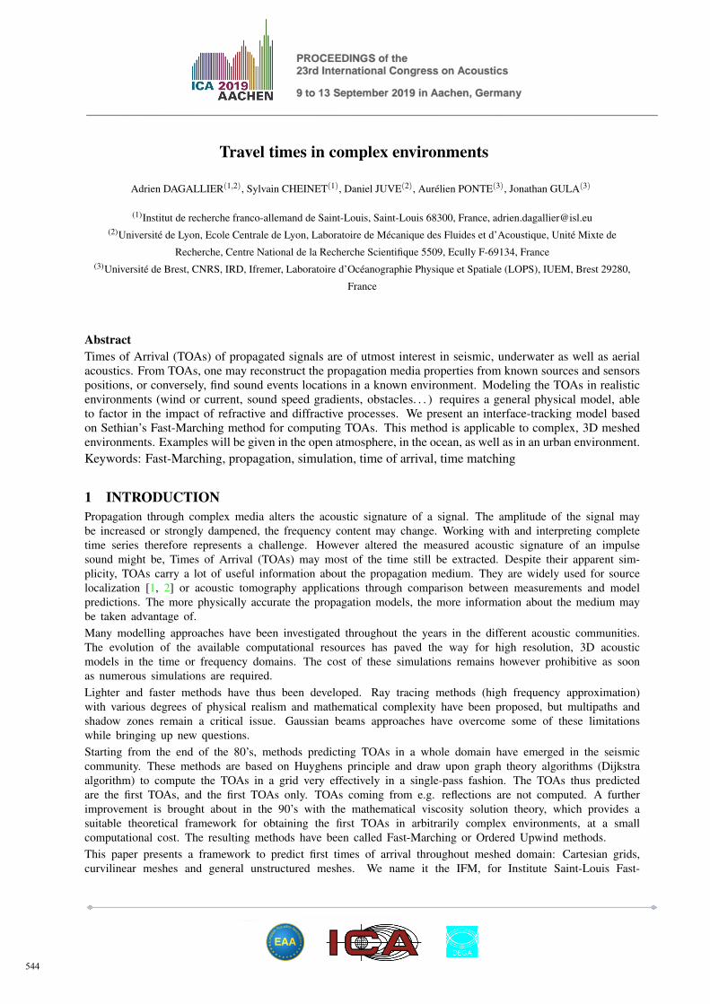
Figure 1. (a-c) Examples of measured atmospheric profiles somewhere in North Germany, in February. (d)Propagation of acoustic wavefronts in the atmosphere defined by the (a-c) data (blue wavefront) and the (a-c)data with reversed wind (yellow wavefront). The simulation domain is 20 km×10 km×4 km in the y, z and xdirection, respectively.

• in a complex atmosphere,

• in the ocean,

• in an urban environment.

3.1 AtmosphereThe model of the previous section is run here on a 40 million points 20 km×10 km×4 km Cartesian domain.The computation takes a few minutes on a single CPU. Second order upwind finite difference are used [5]. Theneighbors of any given points are one grid step away in each dimension, the matrix P is diagonal.The atmosphere through which the wavefronts propagate is shown on Figure 1. The curvature of the wavefrontsmay be linked to the changes in the wind and temperature profiles. It is thus possible to account for theanisotropic effect of the wind on sound propagation. As mentioned in the previous section, an analytical solutionis possible in the absence of wind, which drastically improves the speed of the calculation (from about 130,000points/s to more than 1 million points/s).The wavefronts propagate in an atmosphere with an upward refracting atmosphere due to the sound speed profileand the wind profiles up to 6 km. This creates a so-called shadow zone. As opposed to ray tracing techniques,

546

c (m/s)

1550

1500

1450

(a) (b)

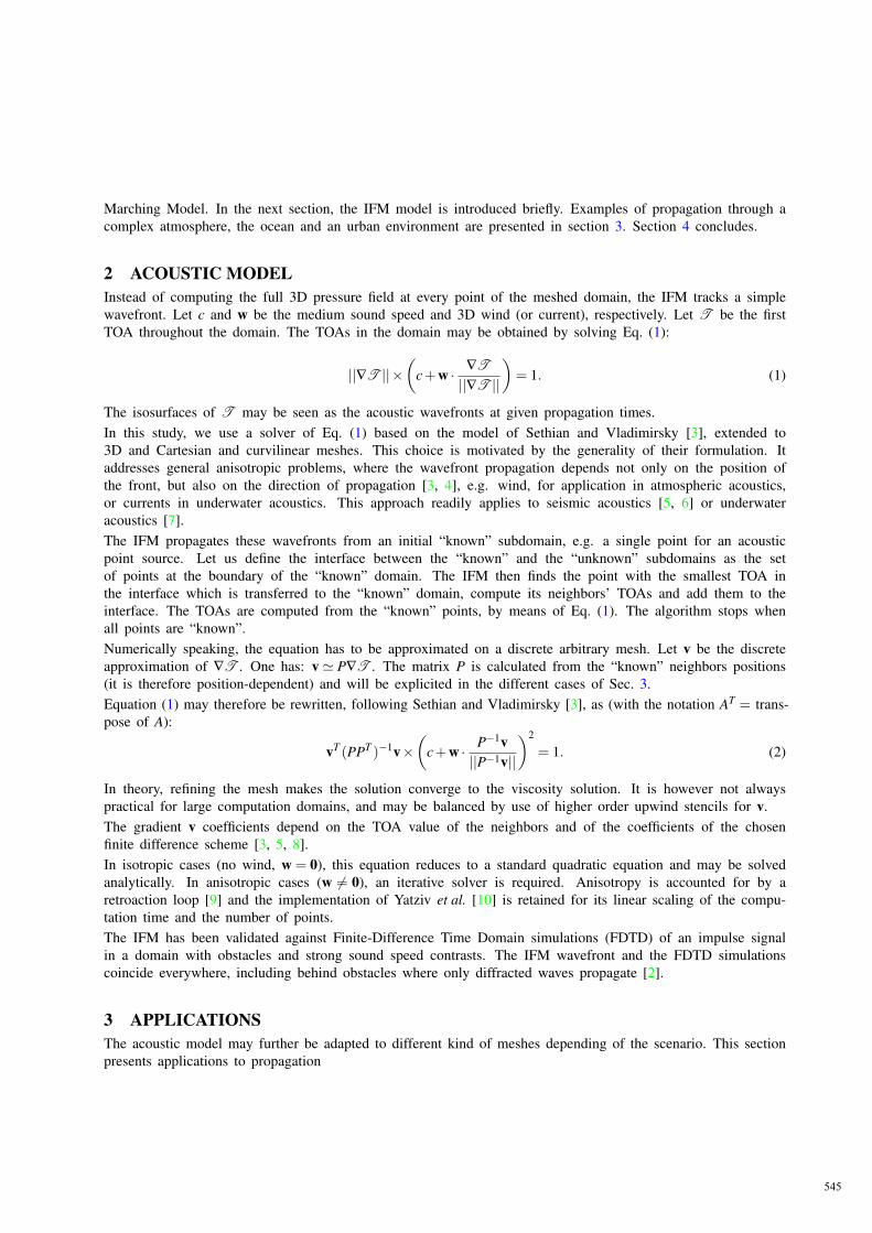
Figure 2. (a) Sound speed c in the ocean, close to the US Eastern coast. The vertical dimension has beenstretched by a factor 50. (b) Snapshots of the acoustic wavefront from an impulse source close to (40N,−68W )after 70, 200 and 330 seconds of propagation.

the IFM is able to predict TOAs in these regions. However, only the wavefront is computed. Informationregarding the amplitude is not accounted for by the model. It is therefore possible that the model would predictTOAs that might not actually be measured, depending on the frequency content of a given signal, or on howdeep into the shadow zone the receiver is. A prior physical analysis is required to define the region in whichthe model results are meaningful for comparison to experimental data.

3.2 OceanThe method is now applied to first TOA determination in the ocean. The sound speed data from Figure 2aare the output of a realistic ROMS simulation for a 1000 km×800 km region, close to the US East coast.The simulation domain has 2000×1600 points and 50 terrain-following veritcal levels. It is forced by realisticsurface forcings and boundary ocean data from a coarser resolution model. More details may be found in Gulaet al. [11]. The high sound speed at the surface is due to the warm Gulf Stream current off New England. Thedata are given on a 160 million points terrain-following curvilinear mesh, and also include the 3D velocity field(not shown).The IFM is extended to curvilinear meshes for propagation on terrain-following meshes. The formalism isexactly the same as in the previous sections. Only the matrix P changes, and must now be expressed in term ofthe Jacobian matrix of the curvilinear transform [12]. The computation time on a single CPU, is of around 90minutes (30,000 points/s), due to the heavier computations involved (Jacobian matrices to inverse) and to ourspecific implementation, which prioritizes low memory usage over efficiency. The code runs on a 16GB laptop.An example of point source propagation is illustrated on Figure 2b. The “creasing” on the wavefronts is causedby the heterogeneity of the sound speed distribution. Even if the oceanic velocities are much smaller than thesound speed (< 1m/s nearly everywhere vs. 1500 m/s), the propagation anisotropy may be observed as in theatmospheric case. It may therefore possible to use the IFM for acoustic tomography of the ocean.

3.3 Urban environmentsThe method is now applied to an urban propagation scenario. The considered domain is of size 170 m×170 m×20 m (Figure 3). To take into account the variety and the complexity of the shape of the building, extensionof the IFM to unstructured meshes is carried out, extending ref. [3] to 3D. The matrix P rows now contain thevectors connecting the current point to its neighbors.As the algorithm requires only the list of the neighbors for each mesh point, the mesh may feature any kindof 3D element (tetrahedron, pyramid, hexahedron...). High order gradient computations are however much more

547

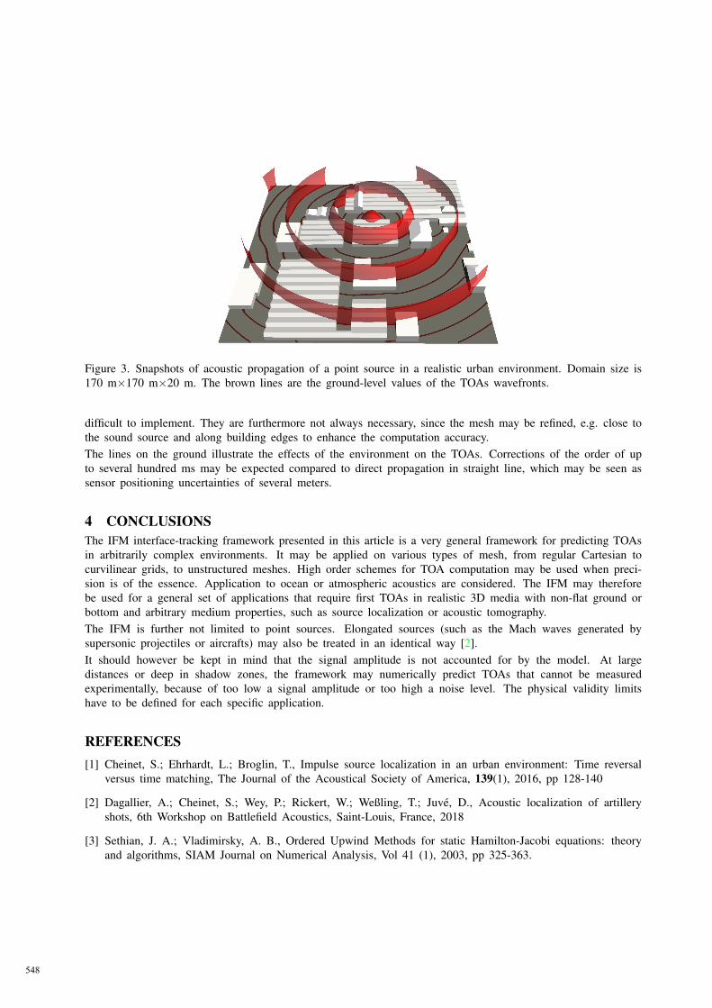
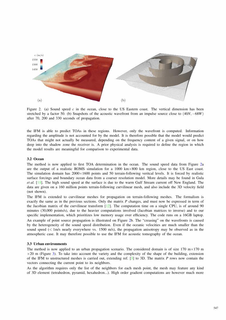
Figure 3. Snapshots of acoustic propagation of a point source in a realistic urban environment. Domain size is170 m×170 m×20 m. The brown lines are the ground-level values of the TOAs wavefronts.

difficult to implement. They are furthermore not always necessary, since the mesh may be refined, e.g. close tothe sound source and along building edges to enhance the computation accuracy.The lines on the ground illustrate the effects of the environment on the TOAs. Corrections of the order of upto several hundred ms may be expected compared to direct propagation in straight line, which may be seen assensor positioning uncertainties of several meters.

4 CONCLUSIONSThe IFM interface-tracking framework presented in this article is a very general framework for predicting TOAsin arbitrarily complex environments. It may be applied on various types of mesh, from regular Cartesian tocurvilinear grids, to unstructured meshes. High order schemes for TOA computation may be used when preci-sion is of the essence. Application to ocean or atmospheric acoustics are considered. The IFM may thereforebe used for a general set of applications that require first TOAs in realistic 3D media with non-flat ground orbottom and arbitrary medium properties, such as source localization or acoustic tomography.The IFM is further not limited to point sources. Elongated sources (such as the Mach waves generated bysupersonic projectiles or aircrafts) may also be treated in an identical way [2].It should however be kept in mind that the signal amplitude is not accounted for by the model. At largedistances or deep in shadow zones, the framework may numerically predict TOAs that cannot be measuredexperimentally, because of too low a signal amplitude or too high a noise level. The physical validity limitshave to be defined for each specific application.

REFERENCES[1] Cheinet, S.; Ehrhardt, L.; Broglin, T., Impulse source localization in an urban environment: Time reversal

versus time matching, The Journal of the Acoustical Society of America, 139(1), 2016, pp 128-140

[2] Dagallier, A.; Cheinet, S.; Wey, P.; Rickert, W.; Weßling, T.; Juvé, D., Acoustic localization of artilleryshots, 6th Workshop on Battlefield Acoustics, Saint-Louis, France, 2018

[3] Sethian, J. A.; Vladimirsky, A. B., Ordered Upwind Methods for static Hamilton-Jacobi equations: theoryand algorithms, SIAM Journal on Numerical Analysis, Vol 41 (1), 2003, pp 325-363.

548

[4] Sethian, J. A, A fast marching level set method for monotonically advancing fronts, Proceedings of theNational Academy of Sciences, 93(4), 1996, pp 1591-1595

[5] Popovici A.; Sethian, J. A, 3D imaging using higher order Fast Marching travel times, Geophysics, 67(2),2002, pp 604-609

[6] Sethian, J. A; Popovici A., 3D travel time computation using the Fast Marching method, Geophysics, 64(2),1999, pp 516-523

[7] Pailhas, Y.; Petillot, Y., Multi-dimensional Fast-Marching approach to wave propagation in heterogeneousmultipath environment, Third Underwater Acoustics Conference and Exhibition, Platanias, Crete, Greece,2015

[8] Sethian, J. A; Vladimirsky, A. B., Fast methods for the Eikonal and related Hamilton-Jacobi equations onunstructured meshes, Proceedings of the National Academy of Sciences, 97(11), 2000, pp 5699-5703

[9] Konukoglu, E.; Sermesant, M.; Clatz, O.; Peyrat, J.-M.; Delingette, H.; Ayache, N., A recursive anisotropicFast Marching approach to reaction diffusion equation: application to tumor growth modeling, In: Karsse-meijer, N., Lelieveldt B. (eds) Information Processing in Medical Imaging, 2007, Lecture Notes in ComputerScience, vol. 4584, Springer Berlin Heidelberg

[10] Yatziv, L.; Bartesaghi, A.; Sapiro, G., O(N) implementation of the fast marching algorithm, Journal ofComputational Physics, 212(2), 2006, pp 393-399

[11] Gula, J.; Molemaker, M. J.; McWilliams, J. C., Gulf stream dynamics along the Southeastern U.S.Seaboard, Journal of Physical Oceanography, 45(3), 2015, 690-715

[12] Visbal, M.; Gaitonde, D., On the Use of Higher-Order Finite-Difference Schemes on Curvilinear and De-forming Meshes, Journal of Computational Physics, 181(1), 2002, pp 155-185

549