1/21

Tutorial for SHAPE v.1.3 Dec. 2006

Hiroyoshi Iwata

“SHAPE” is a package of programs for evaluating biological contour shapes based on elliptic Fourier descriptors (EFDs). This package contains programs for image­processing and contour recording, derivation of EFDs, principal component analysis of EFDs, and visualization of shape variations estimated by the principal components. This tutorial gives you instructions on how to install “SHAPE” and how to try out “SHAPE” with sample files.

! Caution ­ If you have been a user of the older version of SHAPE, please beware of the following point:

I found a bug in SHAPE ver.1.2, which has been fixed in SHAPE ver.1.3. Because of this bug, chain­code obtained by SHAPE ver.1.2 traces an object's contour “clockwise”, although it is expected to trace a contour “counter­clockwise” in general (you can check the direction of contour trace by the viewer programs, ChcViewer and NefViewer). EFDs derived from clockwise chain­code are different from ones derived from counter­clockwise code in the sign of coefficients b and d. As indicated in Table 1, the difference in the sign of the coefficients may not cause any serious problem in the shape analyses, if all EFD or chain­code data are obtained by the same version of SHAPE. However, it should cause a serious artifact, if you analyze jointly the data obtained by the different version of SHAPE. Please be sure NEVER TO ANALYZE JOINTLY EFD or chain­code data obtained by THE DIFFERENT VERSION OF SHAPE! For the joint analysis, please use converter programs to convert the direction of contour trace of chain­code or EFDs obtained by SHAPE ver.1.2.

I greatly apologize for the inconvenience.

Table 1. Direction of contour trace and problems in shape analyses

EFD and chain­code Data

Direction of contour trace Problems in shape analyses Ways of coping

Data obtained by SHAPE ver.1.2 Clockwise No problem Not necessary

Data obtained by SHAPE ver.1.3 Counter­clockwise Of course, No problem Not necessary

Combined data obtained by both versions

The mixture of clockwise and contour­clockwise

The difference in the direction of contour trace causes the difference in the sign of Fourier coefficients b and d. This should cause a serious artifact in the analyses

Use converter programs before analyzing the conbined data

2/21

How to install “SHAPE”

Fig.1

1. Create a new folder named “shape” in your computer (Fig. 1). 2. Extract all the files contained in “shape.zip” to the “shape” folder.

Fig. 2 3. (Optional) For convenience, make short cuts to "ChainCode.exe", "Chc2Nef.exe",

"PrinComp.exe" and "PrinPrint.exe" on your desktop (Fig. 2).

Create a new folder named “shape” and extract all the files contained in “shape.zip” *.

(Optional) Make short cuts to “ChainCode.exe”, “Chc2Nef.exe”, “PrinComp.exe” and “PrinPrintexe”.

* In the case of the version of “SHAPE” distributed by floppy disks, extract all the files contained in “shape1.zip” (disk1) and “shape2.zip” (disk2).

3/21

How to try out “SHAPE” with sample files

This session gives instructions on how to try out “SHAPE” with the sample files contained in the package. First, please try out “ChainCoder” with the sample file named “Sample_img.bmp” which contains the image of five radish roots. “ChainCoder” extracts the contours of objects and stores the relevant information as chain­code. Next, please try out “Chc2Nef” with the sample file named “Sample_chc.chc” which contains chain­code data of c.a. 150 radish roots, or with the output file which you will make as a result of trying out “ChainCoder”. “Chc2Nef” provides the normalized elliptic Fourier descriptors (NEFDs) from chain­coded contours. Finaly, please try out “PrinComp” and “PrinPrint” with the sample file named “Sample_nef.nef” which contains sufficient number of NEFDs data (276 radish roots) for principal component analysis. “PrinComp” performs the principal component analysis of the coefficients of the EFD, and “PrinPrint” visualizes the shape variation accounted for by each principal component. I hope that you become skilled in using “SHAPE” for your own samples through the practice of this tutorial.

First Step: Try out “ChainCoder”

Fig.3 1. Start ChainCoder with double­clicking the “ChainCoder” icon (Fig. 3).

Double­click this icon.

4/21

Fig. 4 2. Set or confirm the analysis parameters as follows (A­E) (Fig. 4).

A) Object Color ­> Dark (Default) B) Scale Included ­> Yes (Default) C) Scale Size ­> 50 x 50 (mm) (Click up arrows) D) Scan Direction ­> Y (Default) E) Scale position ­> Top (Default)

3. Click the “Proceed to Processing” button (Fig. 4).

Change here from 30 x 30 to 50 x 50 by clicking up arrows.

Click this button after setting the parameters.

5/21

Fig. 5 4. Select the image file(s) that you are going to analyze as follows (A­C) (Fig. 5).

A) Click the “Sample_img.bmp” contained in the shape folder. B) Click the [>] button, and “Sample_img.bmp” will appear in the "Selected

File(s)" box. C) Click the “OK” button.

Fig. 6

5. Click the “Load Image” button to load the image into the program (Fig. 6).

A) Click “Sample_img.bmp” to highlight the file.

C) Click this button after selecting the file(s).

B) Click this button to select the file(s) high­lighted in the “File(s)” box.

Click the “Load Image” button.

6/21

Fig. 7 6. (Optional) If you want to process the part of the image, select the processing area as

follows (A­C) (Fig. 7) A) Click the “Select Area” button, and the mouse cursor will change shape from an

arrow to a cross in the image window. B) Push down the left mouse button, drag with the button down and release the

button when the desired area has been delineated. C) Click the "Select" from this popup menu to clip the marked area.

(Optional) A) Click the “Select Area” button.

(Optional) B) Push down the left mouse button, drag with the button down and release the button when the desired area has been delineated.

(Optional) C) Click the "Select" from this popup menu to clip the marked area.

7/21

Fig. 8

7. Click the “Gray Scale” button to change a full color bitmap image to gray­scale.

! Attention: This program can only handle FULL COLOR (24 bits) BITMAP

images, and cannot handle directly 256 COLOR, 16 COLOR and MONOCHROME BITMAP images or JPEG images. So, if you have files of images in a different format, such as jpeg or less colored bitmap (black and white, 16 colors or 256 colors bitmap), you have to convert them to full color (24 bits) bitmap format prior to analysis using the graphic programs such as “Microsoft Paint” that comes with Microsoft Windows.

Fig. 9 Fig. 10

8. Click the “Make Histogram” button (Fig. 9), and a histogram of the gray scale of the pixels will then be shown in the histogram box (Fig. 10). Through this step, an appropriate threshold value is determined and appeared in the box beside the “Binarize Image” button.

Click the “Gray Scale” button.

Click the “Make Histogram” button.

A histogram of the gray scale of the pixels. In this case, the left and right peaks represent the pixels included in the objects and the background, respectively.

8/21

Fig. 11

9. Click the "Binarize Image" button, to convert the gray scale image to a binary image in which the objects and background are represented as 1 (white) and 0 (black), respectively (Fig. 11). If you want to adjust threshold value for the binarization, change the value in the box beside the "Binarize Image" button by clicking the up or down buttons, as appropriate (Fig. 11). The value can be changed by dragging the pointer on the ruler bar below the histogram box (Fig. 10).

Fig. 12 Fig. 13

10. (Optional) Change the number of iteration of the operation from “1” to “3” and click the “Ero Dil Filter” button (Fig. 12). Then, the noises and the thin part of the roots will be removed (Fig. 13).

Fig. 14

11. Click the “Labeling Object” button (Fig. 12), and each object will then be numbered and displayed in the “Chain Code Data” window (Fig. 14).

Click the “Binarize Image” button.

(Optional) Change the number of iteration of the operation to “3” and then click the “Ero Dil Filter” button.

The thin part of the root is removed

after the operation.

Click the “Labeling Object” button.

9/21

Fig. 15

Fig. 16 12. Click the "Chain Coding" button, to obtain the chain­code for each object (Fig. 15).

The chain­code obtained will be displayed in the “Chain Code Data” window (Fig. 16).

Fig. 17 13. Click the "Save to File" button, the chain code data will then be saved in an output

file. In the first time the button is used after executing this program, the "Save Chc File dialog" window will appear. Input the name of the output file as, for example, “test.chc” and save the data. After saving the data for the first image, you can also process remaining multiple files with repeating the steps 5 to 13. Detail information for processing multiple files is described in the manual of SHAPE v.1.3.

14. Close “Chain Coder”.

Click the “Chain Coding” button.

Chain­code obtained.

Click the “Save to File” button.

10/21

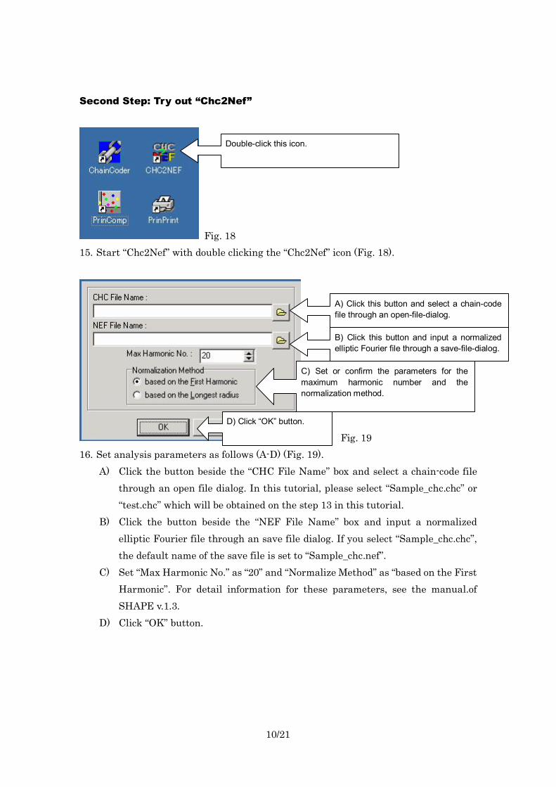
Second Step: Try out “Chc2Nef”

Fig. 18 15. Start “Chc2Nef” with double clicking the “Chc2Nef” icon (Fig. 18).

Fig. 19 16. Set analysis parameters as follows (A­D) (Fig. 19).

A) Click the button beside the “CHC File Name” box and select a chain­code file through an open file dialog. In this tutorial, please select “Sample_chc.chc” or “test.chc” which will be obtained on the step 13 in this tutorial.

B) Click the button beside the “NEF File Name” box and input a normalized elliptic Fourier file through an save file dialog. If you select “Sample_chc.chc”, the default name of the save file is set to “Sample_chc.nef”.

C) Set “Max Harmonic No.” as “20” and “Normalize Method” as “based on the First Harmonic”. For detail information for these parameters, see the manual.of SHAPE v.1.3.

D) Click “OK” button.

Double­click this icon.

A) Click this button and select a chain­code file through an open­file­dialog.

B) Click this button and input a normalized elliptic Fourier file through a save­file­dialog.

C) Set or confirm the parameters for the maximum harmonic number and the normalization method.

D) Click “OK” button.

11/21

Fig. 20 17. Click the "Start" button (Fig. 20). The chain code of the first object is then converted

to the normalized elliptic Fourier descriptors (NEFDs) and the NEFDs and the contour reconstructed by the NEFDs will be appeared in the window (Fig. 21).

Click the “Start”

button.

12/21

Fig. 21 18. (Optional) Click “Turn 180deg” button if you need to turn the object (Fig. 21).

19. (Optional) If you don't want to save the object, click the "Discard" button (Fig. 21).

20. Click “Save/Next” button. Then, the NEFDs obtained will be saved to the output file and the chain­code of the next object will be converted to normalized elliptic Fourier descriptors (Fig. 21). To convert the remaining objects, repeat the steps 18 and 19 until all the objects have been converted.

21. Close “Chc2Nef”.

Click “Save/Next” button.

(Optional) Click “Turn 180deg” button if you need to turn the object.

The contour reconstructed by the NEFDs.

The contour recorded by chain­code.

NEFDs.

Chain­code

Data name

(Optional) Click “Discard” button if you want to save the object.

13/21

Final Step: Try out “PrinComp” and “PrinPrint”

Fig. 22 22. Start “PrinComp” with double clicking the “PrinComp” icon (Fig. 22).

Fig. 23

23. Click “open­file” button (Fig. 23). An open­file­dialog will appear. Then select the sample file named “Sample­nef.nef”. (You can also select the normalized elliptic Fourier file obtained through this tutorial. In that case, the result of principal component analysis will, however, not be meaningful because the number of samples will be small for principal component analysis.)

Fig. 24

Double­click this icon.

Click this button to open a normalized elliptic Fourier file.

14/21

24. After selecting the normalized elliptic Fourier (NEF) file, The "Nef File Information" window will appear. The "Number of Header Lines", "Number of Harmonics" and "Constant Coefficient" parameters are automatically set according to the information described in the header in the NEF file (Fig. 24).

Fig. 25

25. Click the analysis button to perform principal component analysis (Fig. 25) and “Principal Component Analysis Dialog” (Fig. 26) will be appeared.

Fig. 26 26. Click “OK” button (Fig. 26), and the save file dialog will be appeared. After

specifying the name of a saved file (*.pcr), principal component analysis will be performed and the information window which contains the result of principal component analysis will be appeared (Fig.27).

Click this button to perform principal component analysis.

Click the “OK” button to perform principal component analysis.

15/21

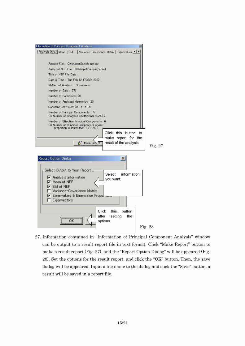
Fig. 27

Fig. 28

27. Information contained in “Information of Principal Component Analysis” window can be output to a result report file in text format. Click “Make Report” button to make a result report (Fig. 27), and the “Report Option Dialog” will be appeared (Fig. 28). Set the options for the result report, and click the “OK” button. Then, the save dialog will be appeared. Input a file name to the dialog and click the "Save" button, a result will be saved in a report file.

Click this button to make report for the result of the analysis

Click this button after setting the options.

Select information you want.

16/21

Fig. 29

28. To calculate the scores of principal components, select "Calculate Prin Score" button (Fig. 29). Then, the "Prin Score Dialog” will appear.

Fig. 30

29. Select the NEFDs file (which is automatically selected by the program) and input the principal component score file name (*.pcs) (this is done automatically by clicking the button beside the box) (Fig. 30). You can also change the number of the components for which the scores are calculated. Then, click the "OK" button. The file will then be saved in tabbed text format and can be opened as a Microsoft Excel worksheet for succeeding analysis from the appropriate (e.g. biological) perspective.

Fig. 31

30. To visualize the shape variation explained by each principal component, click the button with a line­drawing graphic (Fig. 31). After that, the "Reconstruct Contours Dialog" will be appeared.

Click this button to calculate principal component scores.

Click this button to input the name of principal component score file.

Click the “OK” button to output scores to the file.

Click this button to visualize the variations explained by each principal component.

17/21

Fig. 32

31. Select the number of components to be reconstructed through the "Reconstruct Contours Dialog" (Fig. 32). Click the "OK" button, and a save dialog will appear. Input the name of a principal component contours file and click "Save". After that, “PrinPrint” will be automatically executed to display the result and the contours are displayed in a preview form for printing (Fig. 33). If “PrinPrint” cannot be automatically executed, start “PrinPrint” with double clicking the “PrinComp” icon and open the principal component contours file by selecting “Open” from “Files” menu.

Fig 33

Click the “OK” button to save a principal component contours data.

Select the number of component to be reconstructed.

(Optional) Click “Redraw” button if you change the option for drawing.

Click this button to

print contours.

18/21

32. (Optional) You can change some options for drawing the contours, if desired. After setting the draw options, click the "Redraw" button (Fig. 33), the preview window will then be updated in accordance with the new settings.

33. Click the button with a printer icon (Fig. 33), and the print dialog will appear. After setting the printer properties, click the "OK" button. You can then print the contours.

34. Close “PrinComp” and “PrinPrint”.

19/21

Optional Step: Try out “ChcViwer” and “NefViwer”

Fig. 34 35. Start “ChcViewer” (or “NefViewer”) by double­clicking the “ChcViewer” (or

“NefViewer”) icon (Fig. 18).

Fig. 35 36. View the sample’s contour recorded by chain­code (or normalized EFD) data as

follows (A­C) (Fig. 35). A) Select “Open” from the “File” menu, and select a chain­code (or normalized

EFD) file through an open file dialog. In this tutorial, please select “Sample_chc.chc” (or “sample_nef.nef”).

B) Click “Next” button. The contour of the first sample will appear in the window. C) Click “Next” button to draw the contour of the next sample. Click “Back” button

to go back to the previous sample.

Double­click this icon for ChcViewer.

Double­click this icon for NefViewer.

A) Select “Open” item from the “File” menu to open a chain­code (or normalized EFD) file.

B­C) Click “Next” button to draw a sample’s contour recorded by chain­code (or normalized EFD) data. Click “Back” button to go back to the contour drawn previously.

20/21

Fig. 36 37. (Optional) You can change speed for drawing a contour. Select “Speed” from the “Config” menu, the “Speed Setting Dialog” window will appear (Fig. 36). The speed can be changed by dragging the pointer on the ruler bar in the “Speed Setting Dialog” window.

21/21

Through this tutorial, you may become familiar with the process of elliptic Fourier analysis performed by “SHAPE”. Next, please try out “SHAPE” with your own samples. I hope that SHAPE will be used by many researchers in diverse fields and that it will help elucidate various important aspects of biological shapes in the future.

Contact information: Hiroyoshi Iwata (Ph.D) Data­mining and Grid Research Team, National Agricultural Research Center, National Agricultural Research Organization. 3­1­1 Kannondai, Tsukuba, Ibaraki 305­8666, Japan. Tel: +81­29­838­7025; Fax: +81­29­838­8551 E­mail: iwatah@affrc.go.jp Web­page: http://cse.naro.affrc.go.jp/iwatah