Two solvable casesof the Traveling Salesman Problem

Gunter Rothe

Dissertationzur Erlangung des Titels eines Doktors

der technischen Wissenschaften,eingereicht an der Technisch-

Naturwissenschaftlichen Fakultatder Technischen Universitat Graz

Graz, 1988

Betreuer:Prof. Dr. Rainer E. BurkardAdresse:Technische Universitat GrazInstitut fur MathematikKopernikusgasse 24A–8010 Graz

Fur Mareike

Ich danke meiner Frau fur die Geduld,mit der sie mich wahrend der Arbeitan meiner Dissertation entbehrt hat.

Abstract

In the Euclidean Traveling Salesman Problem, a set of points in the plane is given, andwe look for a shortest closed curve through these lines (a “tour”). We treat two specialcases of this problem which are solvable in polynomial time.

The first solvable case is the N-line Traveling Salesman Problem, where the points lie ona small number (N) of parallel lines. Such problems arise for example in the fabrication ofprinted circuit boards, where the distance traveled by a laser which drills holes in certainplaces of the board should be minimized.

By a dynamic programming algorithm, we can solve the N-line Traveling SalesmanProblem for n points in time nN , for fixed N , i. e., in polynomial time. This extends aresult of Cutler (1980) for 3 lines. The parallelity condition can be relaxed to point setswhich lie on N “almost parallel” line segments.

The other solvable case concerns the necklace condition: A tour is a necklace tour if wecan draw disks with the given points as centers such that two disks intersect if and onlyif the corresponding points are adjacent on the tour. If a necklace tour exists, it is theunique optimal tour.

We give an algorithm which tests in O(n3/2) time whether a given tour is a necklace tour,improving an algorithm of Edelsbrunner, Rote, and Welzl (1988) which takes O(n2) time.It is based on solving a system of linear inequalities by the generalized nested dissectionprocedure of Lipton, Rose, and Tarjan (1979). We describe how this method can beimplemented with only linear storage.

We give another algorithm which tests in O(n2 log n) time and linear space, whethera necklace tour exists for a given point set, by transforming the problem to a fractional2-factor problem on a sparse bipartite graph.

Both algorithms also compute radii for the disks realizing the necklace tour.

1

Introduction

The Traveling Salesman Problem is one of the most important problems in the area ofcombinatorial optimization. It asks for computing a tour in a weighted graph (that is, acycle that visits every vertex exactly once) such that the sum of the weights of the edgesin this tour is minimal. A whole monograph, edited by Lawler, Lenstra, Rinnooy Kan,and Shmoys [1985] has been devoted to this problem.

The traveling salesman problem is known to be NP-hard (see Garey and Johnson [1979]or Johnson and Papadimitriou [1985]) which implies that no algorithm is known currentlywhich finds an optimal tour in polynomial time. There are two approaches to circumventthis difficulty: one is the design of algorithms which compute tours that are close tooptimal; the other identifies restricted classes of the problem for which efficient solutionsare possible.

In this thesis, we use the second approach, and we identify two such classes withpolynomial-time solutions. An overview of many other efficiently solvable cases can befound in Gilmore, Lawler, and Shmoys [1985]. Both classes that we treat are subclassesof the Euclidean Traveling Salesman Problem in the plane where the considered graph G

is the complete distance graph of a finite set P of points in the plane: the vertices of G

are the points in P and the weight of an edge between two vertices is the Euclidean dis-tance between the corresponding points. Geometrically, the Euclidean Traveling SalesmanProblem can be formulated as the problem of finding a polygon of shortest length whosevertices are the given points.

A simple polygon is a polygon in which no two sides have a point in common exceptfor the common endpoint of two adjacent sides. The following lemma is an immediateconsequence of the triangle inequality:

Lemma 1. Unless all points lie on one line the optimal tour is a simple polygon having

the given points as vertices.

Although the Euclidean traveling salesman problem is a restricted version of the generaltraveling salesman problem, it is still NP-hard (see Papadimitriou [1977]). There are a fewnatural classes of point sets, however, which allow for an efficient construction of optimaltours. For example, the boundary of the convex hull of P forms the unique optimal tourof P if it contains all points of P .

The first solvable case of the Traveling Salesman Problem that we are going to dealwith is the N-line Traveling Salesman Problem, in which the points lie on N parallel lines,where N is a small number. Such problems arise for example in the fabrication of printedcircuit boards, where a laser drills holes in certain places of a board, and the total distancetraveled by the laser is to be minimized (cf. Lin and Kernighan [1973]).

By the design, the positions of the holes are naturally aligned on parallel lines.

As will be shown in Chapter 1, the N-line Traveling Salesman Problem can be solved inpolynomial time, for fixed N . (The degree of the polynomial is N). The condition that thelines are parallel can be relaxed a little: The points may lie on a set of N “almost parallel”line segments without destroying the properties that are required for our algorithm to work

2

correctly. An exact characterization of those line segments is given in the last section ofChapter 1.

The other class of point sets considered here is based on the notion of the necklacecondition:

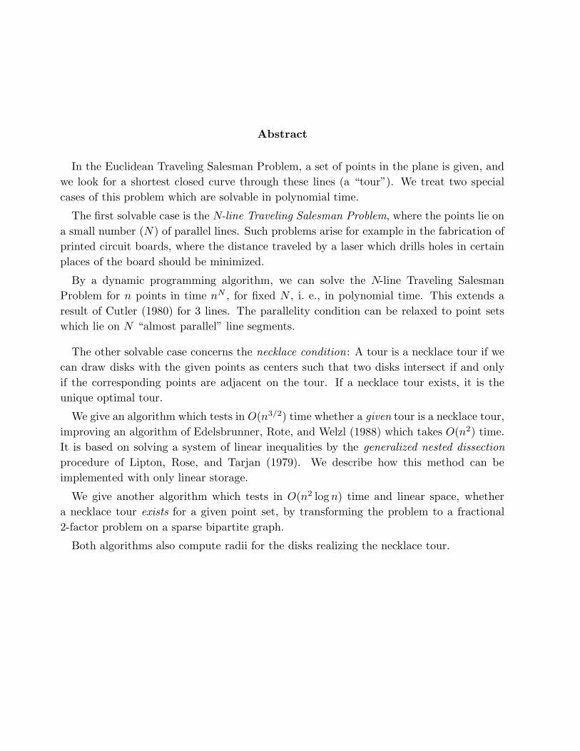
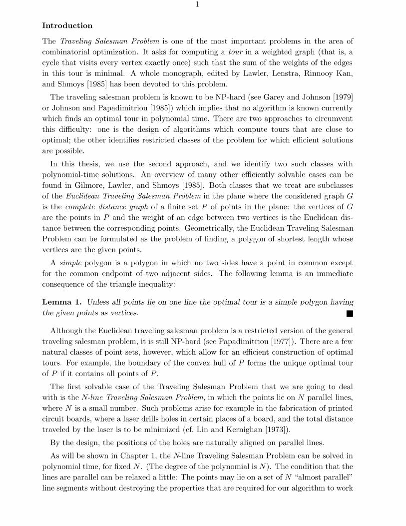
Let P be a finite point set in the plane. A tour T of P is a necklace-tour if it isthe intersection graph of a set S of closed disks centered at the points in P . If anecklace-tour exists, then we say that P satisfies the necklace condition.

Figure 1 shows two examples of necklace-tours: a typical “necklace” which illustratesthe name of the necklace condition, and a more general example. It has been shown bySanders [1968] (see Supnick [1970]) that the traveling salesman problem becomes easy if anecklace-tour exists, since a necklace-tour is the unique optimal tour.

CCCeeePPPP

%%CCCC

@@@

``

&%'$

&%'$

&%'$

&%'$&%

'$&%'$&%

'$&%'$

&%'$

&%'$

&%'$

&%'$

q q q qq

qqqqq

qq

!!!!!@@

@@\

\\

\EEEEEE

,,

,,hhhhhhq

q q

qq

qq

Figure 1. Two necklace tours

The necklace condition is probably not so interesting from the point of view of practicalapplications, but rather because of the nice characterizations which can be obtained andbecause of the algorithmic questions that arise naturally: Find out whether a set of pointsadmits a necklace-tour and if yes, find this tour. Chapter 2 deals with this question.

In Section 2.1 we deal with the easier problem of determining whether a given tour isa necklace tour. This problem is solved by formulating a system of inequalities whosefeasibility has to be checked. This check is carried out by an elimination scheme calledgeneralized nested dissection.

In Section 2.2, we consider the problem of testing the necklace condition and finding anecklace tour.

Some results of Chapter 2 (Sections 2.1.1, 2.1.2, 2.1.3.1, and 2.2) originated in cooper-ation with Herbert Edelsbrunner and Emo Welzl, and they have been published jointly(Edelsbrunner, Rote, and Welzl [1987]).

3

For an overview of the results obtained in this thesis and their relation to previous resultssee the individual introductions to the two chapters.

Notational conventions

When we are talking about a subgraph of the complete distance graph, we shall notdistinguish between the graph and its edge set. This leads to no confusion since the vertexset is always the set P = p1, p2, . . . , pn of given points. In particular, |G| will alwaysdenote the number of edges of the graph G, and we will write “pi, pj ∈ G” for “pi, pjis an edge of the graph G”.

The Euclidean distance between two points X and Y of the plane will be denoted bydist(X, Y ). For the distance between two given points pi and pj we will use the shorternotation dij := dist(pi, pj).

4

Chapter 1: The N-line Traveling Salesman Problem

1.1. Introduction

In this chapter we will deal with the Traveling Salesman Problem in which all points lieon N parallel (or “almost parallel”) lines. We will use a dynamic programming approachto obtain a polynomial algorithm. Our algorithm is an extension of an algorithm byCutler [1980] for three parallel lines. (For two lines, the problem is trivial.) Cutler alsoconsidered the Traveling Salesman Path Problem. A similar but easier special case wasconsidered by Ratliff and Rosenthal [1983]: the problem of order-picking in a rectangularwarehouse. These authors also used the dynamic programming paradigm for their problemand obtained a linear-time algorithm. Cornuejols, Fonlupt, and Naddef [1985] extend theresult of Ratliff and Rosenthal to the Steiner Traveling Salesman Problem for arbitraryundirected series-parallel graphs. In the Steiner Traveling Salesman Problem, we look fora closed path which visits each of a given subset of the vertices at least once. The algorithmtakes linear time.

Another similar algorithm was given in Gilmore, Lawler, and Shmoys [1985], Section 15,for the Traveling Salesman Problem with limited bandwidth. That algorithm also haslinear running time (for fixed bandwidth).

Cutler’s N-line Traveling Salesman Problem has recently been generalized in a differentdirection by Deıneko, van Dal, and Rote [1994]. They considered the problem where thegiven points lie on the boundary of a convex polygon and on one additional line segmentinside this polygon. Clearly, this class of problems contains the 3-line Traveling SalesmanProblem as a special case. Moreover, they improved the complexity from O(n3) to O(n2).†

Our condition that the lines are parallel can be relaxed, and the algorithm can be appliedto points on “almost parallel” lines, which still have the same combinatorial properties withrespect to shortest tours.

In the next section we state the exact condition which the lines must fulfill in order thatour algorithm is applicable. A characterization of such sets of line segments by forbiddensub-configurations is deferred to Section 1.6, since it is somewhat peripheral to the maincourse of the paper. In section 2 we continue by stating one simple but essential lemma

† A common generalization of the N-line Traveling Salesman Problem and the convex-hull-and-line Traveling Salesman Problem was considered by Deıneko and Woeginger [1996]: the convex-hull-and-k-line Traveling Salesman Problem, which has k parallel (or “almost parallel”, see thefollowing paragraph) line segments inside the convex hull, whose carrying lines intersect the convexhull in two common edges. The time bound is O(nk+2), which corresponds to the time bound inthis paper.

5

that follows from the conditions that we impose on the lines, and we discuss to what extentthese conditions are necessary for our algorithm. We also formulate the most elementaryfacts about the Traveling Salesman Problem, and we define the required notations. Inparticular, we will define what we mean by a partial solution.

In the third section we derive the main geometric lemma about optimal partial solutions.In Section 1.4, we then formulate a rather standard dynamic programming algorithm,whose correctness is based on that lemma. Finally, in Section 1.5, we analyze the time andspace complexity of the algorithm exactly. We can also deal with other metrics than theEuclidean distance. This and other possible extensions and open problems are discussedin the concluding section 1.7.

In this chapter, the terminology will be more of a geometric nature: We will often speakof line segments, polygons, etc. instead of edges, tours, etc.

1.2. Elementary facts, definitions, and notations

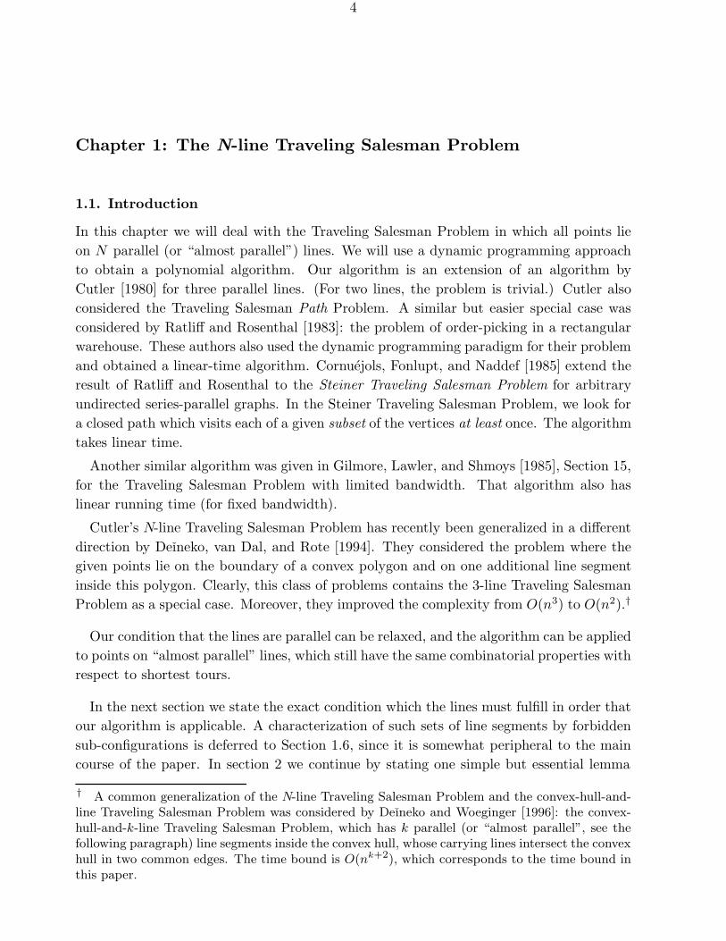
We consider the special case where the points lie on N lines, for a small number N ≥ 2. Weshall assume in the rest of this chapter that N ≥ 2, i. e., not all points lie on a straight line.The algorithm we are going to present works for the case when the lines are parallel, butalso more generally when the points lie on N straight line segments fulfilling the followingcondition:

• No segment is perpendicular to the x-axis.

• For every pair of segments which are not parallel: If we project the twosegments and the intersection of their carrying lines onto the x-axis, theprojection of the intersection lies always outside the projections of the twosegments, never on or between these projections (cf. Figure 2).

- x

hhhhhhhh

hhhhhhhh

hhhhh

bbbb

bbbb

bbbb

bbbb

hhhhhhh

bbbbhhhhhhh

bbbbhhhhhhh

bbbbhhhhhhh

bbbbhhhhhhh

bbbb

Figure 2.

Three line segments which fulfillthe condition for allowed segments

6

Of course, the x-axis can be an arbitrary line, but for definiteness, we have chosen thisformulation.

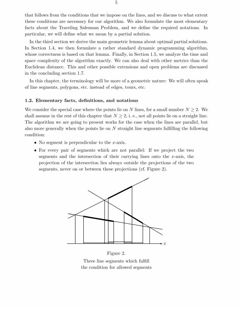
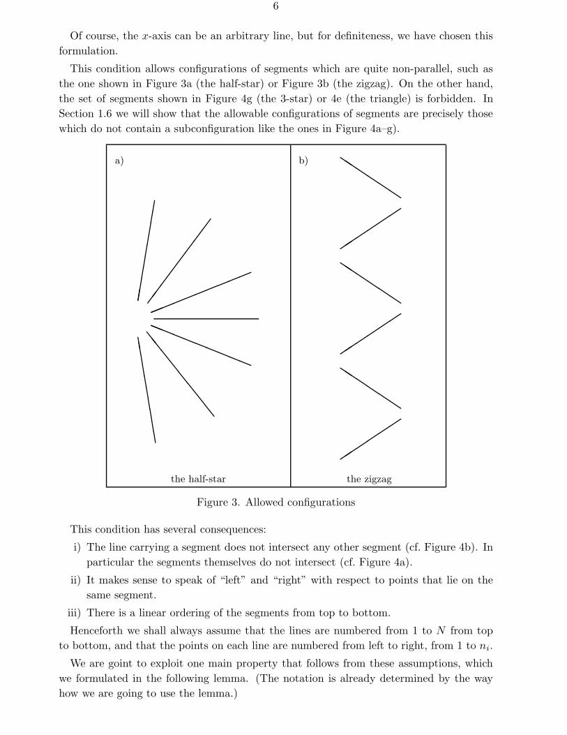
This condition allows configurations of segments which are quite non-parallel, such asthe one shown in Figure 3a (the half-star) or Figure 3b (the zigzag). On the other hand,the set of segments shown in Figure 4g (the 3-star) or 4e (the triangle) is forbidden. InSection 1.6 we will show that the allowable configurations of segments are precisely thosewhich do not contain a subconfiguration like the ones in Figure 4a–g).

a) b)

!!!!!!!!!!

EEEEEEEEEE

aaaa

aaaa

aa

\\\\\\\\

QQ

QQ

QQ

QQ

QQ

QQ

QQ

QQ

QQ

the half-star the zigzag

Figure 3. Allowed configurations

This condition has several consequences:

i) The line carrying a segment does not intersect any other segment (cf. Figure 4b). Inparticular the segments themselves do not intersect (cf. Figure 4a).

ii) It makes sense to speak of “left” and “right” with respect to points that lie on thesame segment.

iii) There is a linear ordering of the segments from top to bottom.

Henceforth we shall always assume that the lines are numbered from 1 to N from topto bottom, and that the points on each line are numbered from left to right, from 1 to ni.

We are goint to exploit one main property that follows from these assumptions, whichwe formulated in the following lemma. (The notation is already determined by the wayhow we are going to use the lemma.)

7

a) d) f)

g)e)

b)

c)

the triangle the 3-star

Figure 4. Forbidden configurations

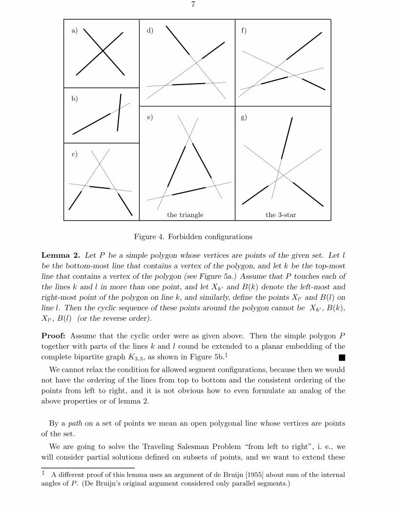
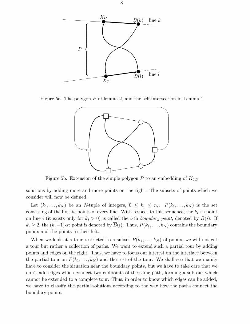
Lemma 2. Let P be a simple polygon whose vertices are points of the given set. Let l

be the bottom-most line that contains a vertex of the polygon, and let k be the top-most

line that contains a vertex of the polygon (see Figure 5a.) Assume that P touches each of

the lines k and l in more than one point, and let Xk′ and B(k) denote the left-most and

right-most point of the polygon on line k, and similarly, define the points Xl′ and B(l) on

line l. Then the cyclic sequence of these points around the polygon cannot be Xk′ , B(k),Xl′ , B(l) (or the reverse order).

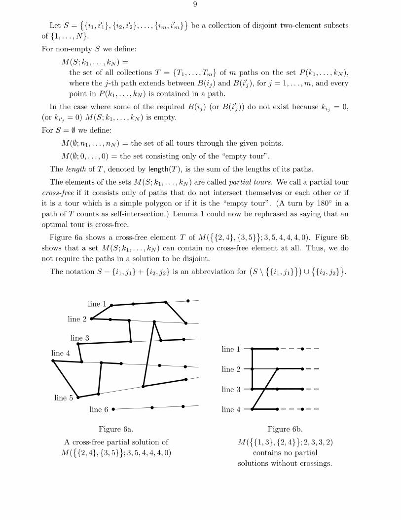
Proof: Assume that the cyclic order were as given above. Then the simple polygon P

together with parts of the lines k and l cound be extended to a planar embedding of thecomplete bipartite graph K3,3, as shown in Figure 5b.‡

We cannot relax the condition for allowed segment configurations, because then we wouldnot have the ordering of the lines from top to bottom and the consistent ordering of thepoints from left to right, and it is not obvious how to even formulate an analog of theabove properties or of lemma 2.

By a path on a set of points we mean an open polygonal line whose vertices are pointsof the set.

We are going to solve the Traveling Salesman Problem “from left to right”, i. e., wewill consider partial solutions defined on subsets of points, and we want to extend these

‡ A different proof of this lemma uses an argument of de Bruijn [1955] about sum of the internalangles of P . (De Bruijn’s original argument considered only parallel segments.)

8

p

v v

vv 1

z

N

P

Xk′B(k)

B(l)Xl′

line k

line l

Figure 5a. The polygon P of lemma 2, and the self-intersection in Lemma 1

hh

h'

&

$

%p

hhhhhhh

((((((

Figure 5b. Extension of the simple polygon P to an embedding of K3,3

solutions by adding more and more points on the right. The subsets of points which weconsider will now be defined.

Let (k1, . . . , kN ) be an N-tuple of integers, 0 ≤ ki ≤ ni. P (k1, . . . , kN ) is the setconsisting of the first ki points of every line. With respect to this sequence, the ki-th pointon line i (it exists only for ki > 0) is called the i-th boundary point, denoted by B(i). Ifki ≥ 2, the (ki−1)-st point is denoted by B(i). Thus, P (k1, . . . , kN) contains the boundarypoints and the points to their left.

When we look at a tour restricted to a subset P (k1, . . . , kN) of points, we will not geta tour but rather a collection of paths. We want to extend such a partial tour by addingpoints and edges on the right. Thus, we have to focus our interest on the interface betweenthe partial tour on P (k1, . . . , kN) and the rest of the tour. We shall see that we mainlyhave to consider the situation near the boundary points, but we have to take care that wedon’t add edges which connect two endpoints of the same path, forming a subtour whichcannot be extended to a complete tour. Thus, in order to know which edges can be added,we have to classify the partial solutions according to the way how the paths connect theboundary points.

9

Let S =i1, i′1, i2, i′2, . . . , im, i′m be a collection of disjoint two-element subsets

of 1, . . . , N.For non-empty S we define:

M(S; k1, . . . , kN ) =the set of all collections T = T1, . . . , Tm of m paths on the set P (k1, . . . , kN ),where the j-th path extends between B(ij) and B(i′j), for j = 1, . . . , m, and everypoint in P (k1, . . . , kN ) is contained in a path.

In the case where some of the required B(ij) (or B(i′j)) do not exist because kij= 0,

(or ki′j = 0) M(S; k1, . . . , kN ) is empty.

For S = ∅ we define:

M(∅; n1, . . . , nN ) = the set of all tours through the given points.

M(∅; 0, . . . , 0) = the set consisting only of the “empty tour”.

The length of T , denoted by length(T ), is the sum of the lengths of its paths.

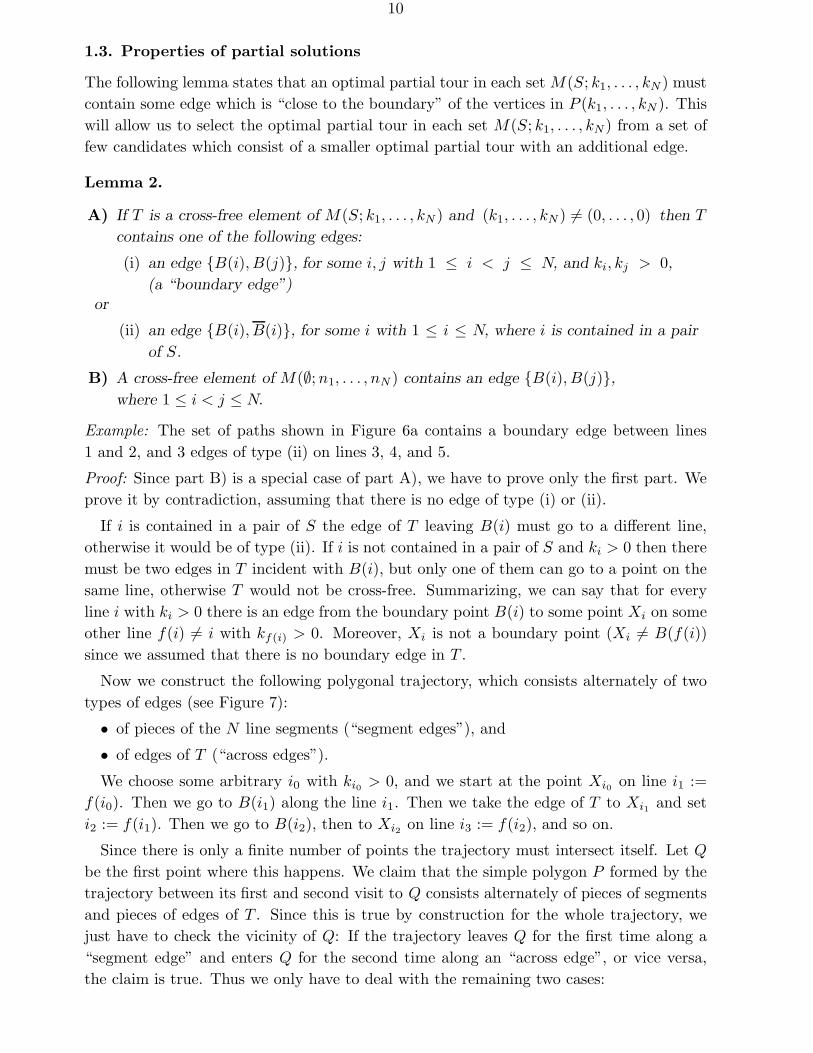
The elements of the sets M(S; k1, . . . , kN ) are called partial tours. We call a partial tourcross-free if it consists only of paths that do not intersect themselves or each other or ifit is a tour which is a simple polygon or if it is the “empty tour”. (A turn by 180 in apath of T counts as self-intersection.) Lemma 1 could now be rephrased as saying that anoptimal tour is cross-free.

Figure 6a shows a cross-free element T of M(2, 4, 3, 5; 3, 5, 4, 4, 4, 0). Figure 6b

shows that a set M(S; k1, . . . , kN) can contain no cross-free element at all. Thus, we donot require the paths in a solution to be disjoint.

The notation S − i1, j1 + i2, j2 is an abbreviation for(S \ i1, j1) ∪ i2, j2.

ssssssss

ssssline 1

line 2

line 3

line 4

sss

ss s

line 1

line 2

line 3

line 4

line 5line 6

s s ss s s s

ssss s s s s

s s ss s

Figure 6a.

A cross-free partial solution ofM(2, 4, 3, 5; 3, 5, 4, 4, 4, 0)

Figure 6b.

M(1, 3, 2, 4; 2, 3, 3, 2)contains no partial

solutions without crossings.

10

1.3. Properties of partial solutions

The following lemma states that an optimal partial tour in each set M(S; k1, . . . , kN ) mustcontain some edge which is “close to the boundary” of the vertices in P (k1, . . . , kN ). Thiswill allow us to select the optimal partial tour in each set M(S; k1, . . . , kN) from a set offew candidates which consist of a smaller optimal partial tour with an additional edge.

Lemma 2.

A) If T is a cross-free element of M(S; k1, . . . , kN ) and (k1, . . . , kN ) 6= (0, . . . , 0) then T

contains one of the following edges:

(i) an edge B(i), B(j), for some i, j with 1 ≤ i < j ≤ N, and ki, kj > 0,

(a “boundary edge”)or

(ii) an edge B(i), B(i), for some i with 1 ≤ i ≤ N, where i is contained in a pair

of S.

B) A cross-free element of M(∅; n1, . . . , nN ) contains an edge B(i), B(j),where 1 ≤ i < j ≤ N.

Example: The set of paths shown in Figure 6a contains a boundary edge between lines1 and 2, and 3 edges of type (ii) on lines 3, 4, and 5.

Proof: Since part B) is a special case of part A), we have to prove only the first part. Weprove it by contradiction, assuming that there is no edge of type (i) or (ii).

If i is contained in a pair of S the edge of T leaving B(i) must go to a different line,otherwise it would be of type (ii). If i is not contained in a pair of S and ki > 0 then theremust be two edges in T incident with B(i), but only one of them can go to a point on thesame line, otherwise T would not be cross-free. Summarizing, we can say that for everyline i with ki > 0 there is an edge from the boundary point B(i) to some point Xi on someother line f(i) 6= i with kf(i) > 0. Moreover, Xi is not a boundary point (Xi 6= B(f(i))since we assumed that there is no boundary edge in T .

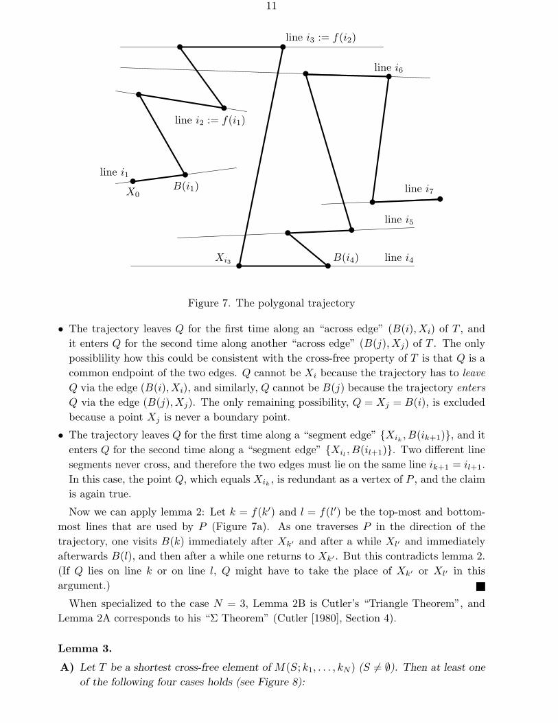
Now we construct the following polygonal trajectory, which consists alternately of twotypes of edges (see Figure 7):

• of pieces of the N line segments (“segment edges”), and

• of edges of T (“across edges”).

We choose some arbitrary i0 with ki0 > 0, and we start at the point Xi0 on line i1 :=f(i0). Then we go to B(i1) along the line i1. Then we take the edge of T to Xi1 and seti2 := f(i1). Then we go to B(i2), then to Xi2 on line i3 := f(i2), and so on.

Since there is only a finite number of points the trajectory must intersect itself. Let Q

be the first point where this happens. We claim that the simple polygon P formed by thetrajectory between its first and second visit to Q consists alternately of pieces of segmentsand pieces of edges of T . Since this is true by construction for the whole trajectory, wejust have to check the vicinity of Q: If the trajectory leaves Q for the first time along a“segment edge” and enters Q for the second time along an “across edge”, or vice versa,the claim is true. Thus we only have to deal with the remaining two cases:

11

tt

t

t ttt

t t

tt

tt

t

line i3 := f(i2)

line i6

line i2 := f(i1)

B(i1)X0

line i1

Xi3 B(i4) line i4

line i5

line i7

Figure 7. The polygonal trajectory

• The trajectory leaves Q for the first time along an “across edge” (B(i), Xi) of T , andit enters Q for the second time along another “across edge” (B(j), Xj) of T . The onlypossiblility how this could be consistent with the cross-free property of T is that Q is acommon endpoint of the two edges. Q cannot be Xi because the trajectory has to leaveQ via the edge (B(i), Xi), and similarly, Q cannot be B(j) because the trajectory entersQ via the edge (B(j), Xj). The only remaining possibility, Q = Xj = B(i), is excludedbecause a point Xj is never a boundary point.

• The trajectory leaves Q for the first time along a “segment edge” Xik, B(ik+1), and it

enters Q for the second time along a “segment edge” Xil, B(il+1). Two different line

segments never cross, and therefore the two edges must lie on the same line ik+1 = il+1.In this case, the point Q, which equals Xik

, is redundant as a vertex of P , and the claimis again true.

Now we can apply lemma 2: Let k = f(k′) and l = f(l′) be the top-most and bottom-most lines that are used by P (Figure 7a). As one traverses P in the direction of thetrajectory, one visits B(k) immediately after Xk′ and after a while Xl′ and immediatelyafterwards B(l), and then after a while one returns to Xk′ . But this contradicts lemma 2.(If Q lies on line k or on line l, Q might have to take the place of Xk′ or Xl′ in thisargument.)

When specialized to the case N = 3, Lemma 2B is Cutler’s “Triangle Theorem”, andLemma 2A corresponds to his “Σ Theorem” (Cutler [1980], Section 4).

Lemma 3.

A) Let T be a shortest cross-free element of M(S; k1, . . . , kN) (S 6= ∅). Then at least one

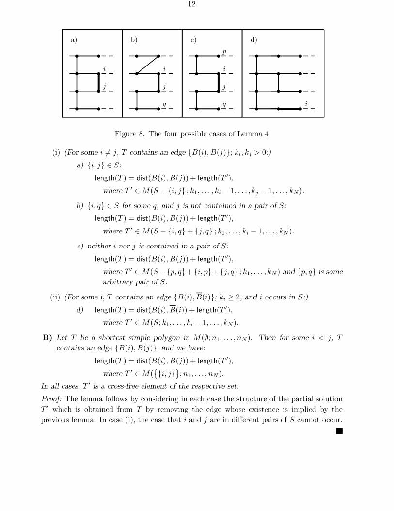
of the following four cases holds (see Figure 8):

12

ssssssssa)

ssssssssb)

ssssssssc)

ssssssssd)

ssssp

i

j

q

i

j

q

i

j

i

Figure 8. The four possible cases of Lemma 4

(i) (For some i 6= j, T contains an edge B(i), B(j); ki, kj > 0:)

a) i, j ∈ S:

length(T ) = dist(B(i), B(j)) + length(T ′),

where T ′ ∈ M(S − i, j ; k1, . . . , ki − 1, . . . , kj − 1, . . . , kN ).

b) i, q ∈ S for some q, and j is not contained in a pair of S:

length(T ) = dist(B(i), B(j)) + length(T ′),

where T ′ ∈ M(S − i, q + j, q ; k1, . . . , ki − 1, . . . , kN).

c) neither i nor j is contained in a pair of S:

length(T ) = dist(B(i), B(j)) + length(T ′),

where T ′ ∈ M(S −p, q+ i, p+ j, q ; k1, . . . , kN ) and p, q is some

arbitrary pair of S.

(ii) (For some i, T contains an edge B(i), B(i); ki ≥ 2, and i occurs in S:)

d) length(T ) = dist(B(i), B(i)) + length(T ′),

where T ′ ∈ M(S; k1, . . . , ki − 1, . . . , kN ).

B) Let T be a shortest simple polygon in M(∅; n1, . . . , nN ). Then for some i < j, T

contains an edge B(i), B(j), and we have:

length(T ) = dist(B(i), B(j)) + length(T ′),

where T ′ ∈ M(i, j; n1, . . . , nN ).

In all cases, T ′ is a cross-free element of the respective set.

Proof: The lemma follows by considering in each case the structure of the partial solutionT ′ which is obtained from T by removing the edge whose existence is implied by theprevious lemma. In case (i), the case that i and j are in different pairs of S cannot occur.

13

1.4. The algorithm

We can now set up a dynamic programming recursion corresponding to the equations inLemma 3 in a straightforward way, involving variables d(S; k1, . . . , kN ) corresponding tothe sets M(S; k1, . . . , kN).

The starting value of the recursion is d(∅; 0, . . . , 0) := 0.

Let S =i1, i′1 , i2, i′2 , . . . , im, i′m and let l1, . . . , lN−2m be the indices that do

not occur in a pair of S, in some fixed order. Then:

If S 6= ∅ and kij= 0 or ki′j = 0 for some 1 ≤ j ≤ m, then we set:

d(S; k1, . . . , kN) := ∞.

Otherwise we set:

d(S; k1, . . . , kN ) := min ∆a, ∆b1, ∆b2, ∆c, ∆d1, ∆d2 ,

where

∆a := min

dist(B(ij), B(i′j)) + d(S−ij , i′j ; k1, . . . , kij−1, . . . , ki′j−1, . . . , kN)

∣∣1 ≤ j ≤ m

∆b1 := min

dist(B(i′j), B(ls)) + d(S−ij , i′j+ ij , ls ; k1, . . . , ki′j−1, . . . , kN )

∣∣1 ≤ j ≤ m, 1 ≤ s ≤ N−2m

∆b2 := min

dist(B(ij), B(ls)) + d(S−ij , i′j+ i′j , ls ; k1, . . . , kij

−1, . . . , kN )∣∣

1 ≤ j ≤ m, 1 ≤ s ≤ N−2m

∆c := min

dist(B(ls), B(lt)) + d(S−ij , i′j+ ij , ls+ i′j , lt ; k1, . . . , kN)∣∣

1 ≤ s, t ≤ N−2m, s 6= t, 1 ≤ j ≤ m

∆d1 := min

dist(B(ij), B(ij)) + d(S; k1, . . . , kij−1, . . . , kN )

∣∣ 1 ≤ j ≤ m, kij≥ 2

∆d2 := min

dist(B(i′j), B(i′j)) + d(S; k1, . . . , ki′j−1, . . . , kN )

∣∣ 1 ≤ j ≤ m, ki′j ≥ 2

(The minimum of an empty set is always taken to be ∞. This ensures that d(∅; k1, . . . , kN)is ∞ unless k = (0, . . . , 0).)

Finally, as an exception to the above rule:

d(∅; n1, . . . , nN) := min

dist(B(i), B(j)) + d(i, j; n1, . . . , nN )

∣∣ 1 ≤ i < j ≤ N.

We have to establish some order in which these recursions can be computed. We couldfor example compute the d(S; k1, . . . , kN ) in increasing lexicographic order of (k1, . . . , kN ).For equal (k1, . . . , kN ), the values with larger cardinality of S are computed first. Anotherpossibility would be to compute them in increasing order of

∑ki − |S|, which is equal to

the number of edges in the elements of M(S; k1, . . . , kN ).

Example: N = 5; (aij denotes the j-th point on line i):

14

d(1, 3; 1, 3, 5, 0, 7) = min

dist(a11, a35) + d(

; 0, 3, 4, 0, 7), (a)

dist(a11, a23) + d(2, 3; 0, 3, 5, 0, 7), (b)

dist(a11, a57) + d(3, 5; 0, 3, 5, 0, 7), (b)

dist(a23, a35) + d(2, 3; 1, 3, 4, 0, 7), (b)

dist(a35, a57) + d(3, 5; 1, 3, 4, 0, 7), (b)

dist(a23, a57) + d(1, 2 , 3, 5; 1, 3, 5, 0, 7), (c)

dist(a23, a57) + d(1, 5 , 2, 3; 1, 3, 5, 0, 7), (c)

dist(a35, a34) + d(1, 3; 1, 3, 4, 0, 7)

(d)

The first line, corresponding to case (a), can be omitted in this case since M(∅; 0, 4, 5, 0, 7)is empty and d(∅; 0, 4, 5, 0, 7) = ∞.

Lemma 4. If M(S; k1, . . . , kN ) 6= ∅, then:

length of theshortest element in

M(S; k1, . . . , kN)≤ d(S; k1, . . . , kN ) ≤

length of the shortestcross-free element inM(S; k1, . . . , kN)

Proof: The left inequality is true since d(S; k1, . . . , kN ) is always the length of some elementfrom M(S; k1, . . . , kN), and the right inequality follows from Lemma 3 by induction on therecursion.

Since for M(∅; n1, . . . , nN ) the left and right sides of Lemma 4 are equal (by Lemma 1)we get

Theorem 5. d(∅; n1, . . . , nN ) is the length of the shortest tour.

Remark: Some impossible cases could be excluded from the recursion. For example, if|S| = 1 then case (a) need not be considered (like in the previous example) except at thevery beginning. However, this would not reduce the running time substantially except forvery small N .

15

1.5. Complexity analysis

Let us now analyze the complexity of the algorithm, both as regards space and time. LetPN denote the number of different sets S, i. e., the number of sets of disjoint unorderedpairs of 1, . . . , N. If we regard the pairs in such a set S as the cycles of a permutation,it is easy to see that PN equals the number of permutations of N elements whose squareis the identity, or equivalently, which are equal to their own inverse.

The numbers PN can be computed by the recursion:

PN+1 = PN + NPN−1 (N ≥ 1) (1)

from the start values P 0 = P 1 = 1. This recursion was given in Rothe [1800], p. 282. Itcan be proved by splitting the PN+1 sets S into those where the element N + 1 is notcontained in a pair and into those where it forms a pair with one of the N other elements.(The very same recursion, but with different start values, occurs in Gilmore, Lawler, andShmoys [1985], p. 138, where it describes the number of equivalence classes of partial toursfor the bandwidth-constrained Traveling Salesman Problem.)

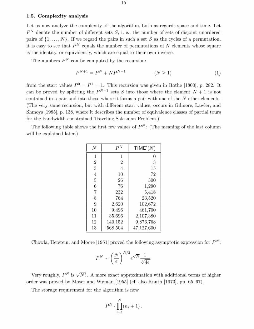
The following table shows the first few values of PN : (The meaning of the last columnwill be explained later.)

N PN TIME′(N)

1 1 02 2 33 4 154 10 725 26 3006 76 1,2907 232 5,4188 764 23,5209 2,620 102,672

10 9,496 461,70011 35,696 2,107,38012 140,152 9,876,76813 568,504 47,127,600

Chowla, Herstein, and Moore [1951] proved the following asymptotic expression for P N :

PN ∼(

N

e

)N/2

e√

N 14√

4e.

Very roughly, PN is√

N ! . A more exact approximation with additional terms of higherorder was proved by Moser and Wyman [1955] (cf. also Knuth [1973], pp. 65–67).

The storage requirement for the algorithm is now

PN ·N∏

i=1

(ni + 1) .

16

Thus, for fixed N , the storage requirement is

O

(N∏

i=1

(ni + 1)

)= O

(N∏

i=1

ni

)= O

(nN),

if we denote the total number of points by n =∑N

i=1 ni.

If n is fixed then the maximum of the left side in the above equation is achieved forni = n/N ; thus, using the inequality ni + 1 ≤ 2ni, the constant of the O-notation in theexpression O(nN ) is at most

( 2N

)N

· PN =( 2

N

)N(N

e

)N/2

e√

N 14√

4e= O

(1

(N/4)N/2· 1eN/2−√

N

),

which decreases quite fast as N increases.

For analyzing the time complexity, let us now establish the complexity of one step of therecursion: If S contains m pairs, then there are at most m, 2m(N−2m), (N−2m)(N−2m−1)m, and 2m terms corresponding to cases (a), (b), (c), and (d), respectively. Therefore,the total number of terms which are necessary for computing d(S; k1, . . . , kN ) is the sumof these four expressions, which is m(3 + N+ N2) + m2(−4N− 2) + 4m3.

Let PNm denote the number of sets S containing exactly m disjoint unordered pairs of

1, . . . , N. It is equal to the number of permutations with m cycles of length 2 and N−2m

cycles of length 1. Therefore, we have

PNm =

N !2mm! (N− 2m)!

, for 0 ≤ m ≤ N/2. (2)

Neglecting the boundary cases, the time complexity is thus

TIME(N) = TIME′(N) ·(

N∏i=1

(ni + 1)

),

where TIME′(N), the time for evaluating d(S; k1, . . . , kN ) for all sets S for some fixedN-tuple (k1, . . . , kN), is given as follows:

TIME′(N) =∑m

PNm · (m(3 + N+ N2) + m2(−4N− 2) + 4m3

). (3)

(By observing that PNm = 0 for m < 0 or m > N/2, we may simplify matters by letting

the summation index m vary over all integers.)

The terms involving the variable m in this sum can be eliminated by using the followingformulas, which follow directly from (2):

PNm m =

N(N−1)2

PN−2m−1

PNm m(m − 1) =

N(N−1)(N−2)(N−3)4

PN−4m−2

PNm m(m − 1)(m − 2) =

N(N−1)(N−2)(N−3)(N−4)(N−5)8

PN−6m−3.

17

After this we can carry out the summation over m, using the identity P N =∑

m PNm , and

express TIME′(N) in terms of N , PN−2, PN−3, . . . , and PN−6. Repeated application ofthe recursion (1) leads then to the following short expression:

TIME′(N) =N(N− 1)

2(PN + PN−2

).

(The calculation is carried out in detail in the original version of the technical reportRote [1988].) The values of TIME′(N) are tabulated in the above table.

Thus, for fixed N , the time complexity is again

O

(N∏

i=1

(ni + 1)

)= O

(N∏

i=1

ni

)= O

(nN).

Arguing as in the case of the storage requirement, we find that the constant of theO-notation in the expression O(nN) is at most

(2N

)N

·(

N

2

)(PN + PN+2

)= O

((2N

)N

N2

(N

e

)N/2

e√

N

)

= O

(1

(N/4)N/2−2· 1

eN/2−√N

).

We summarize our results in the following

Theorem 6. The N-line Traveling Salesman Problem with n1, n2, . . . , nN points on

the lines 1, 2, . . . , N can be solved in space

O

(PN ·

N∏i=1

(ni + 1)

)

and time

O

(PN · N2

N∏i=1

(ni + 1)

),

where the numbers PN are defined by the recursion (1). For fixed N, and for a total

number of n points, the space and time complexities are thus

O(nN).

18

1.6. Characterization of “quasi-parallel” line segments

In Section 1.2, the following property was required of a set of line segments in order thatour algorithm could be applied:

No segment is perpendicular to the x-axis, and for any two segments which are notparallel the projection of the intersection of the two lines carrying the segmentsonto the x-axis lies always outside the projections of the two segments.

We call a set of line segments quasi-parallel, if they can be rotated in such a way thatthis property is fulfilled, in other words, if an appropriate x-axis can be found. In thissection, we give a characterization of this property.

First we have to introduce some terminology:

By an orientation of a line we mean an assignment of the label “left” to one directionof the line and the label “right” to the other direction. An oriented line is a line togetherwith an orientation. When we draw an oriented line the orientation will be indicated byan arrow pointing in the “right” direction.

By an oriented segment we mean a segment a with an orientation of the line g(a) carryingthe segment.

When we project an oriented line on another line which is not perpendicular to it weget a corresponding orientation of the second line in a natural way.

Now we call two oriented segments a and b oriented consistently if the intersection ofthe carrying lines g(a) and g(b) either lies both on the left side of a on g(a) and on the leftside of b on g(b) or on the right side of a resp. b on both g(a) and g(b). (In case a and b

are parallel, the orientations have to be the same in order to be consistent.)

We can now rephrase the above definition of quasi-parallelness in the terminology justintroduced as follows:

There is an oriented line l (this line corresponds to the x-axis in the previousformulation), not perpendicular to any segment, such that for the correspondingorientations of the segments obtained by projection from the orientation of l, anypair of non-parallel segments a and b is oriented consistently.

Theorem 3. Let a set of at least 3 segments be given, and let g0 be any fixed segment

of this set. Then the set of segments is quasi-parallel if and only if every subset of three

segments containing g0 is quasi-parallel.

Proof: First of all, it is clear that consequence (i) of Section 1.2 holds, i. e., the linecarrying a segment does not intersect any other segment, and in particular, the segmentsthemselves do not intersect.

Now fix any orientation of g0. Then there is only one possible orientation of every othersegment which is consistent with the orientation of g0.

We have to show two things:

(a) There is an oriented line l such that the orientations thus constructed correspondby projection to the orientation of l.

19

(b) Every pair of non-parallel segments a and b (different from g0) is also orientedconsistently.

For proving (b), let’s assume that two segments a and b are not oriented consistently.Then the orientation of b resulting from the orientation of g0 is different from the orientationof b resulting from the orientation of a resulting from the orientation of g0; thus, even forthe 3-set g0, a, b, it would be impossible to orient the segments consistently.

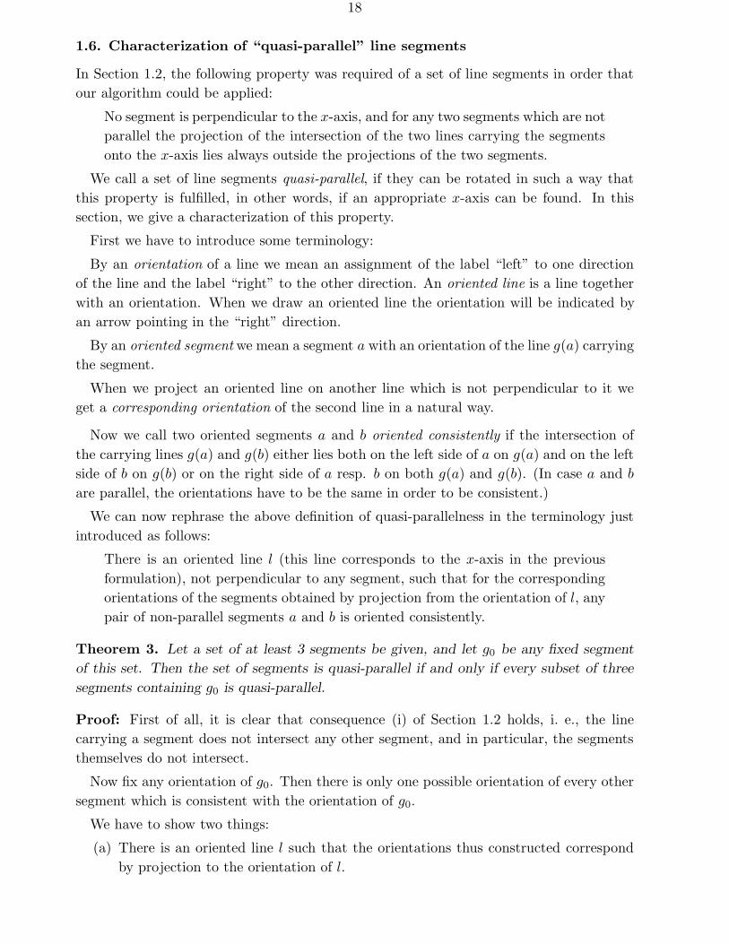
Now we still have to prove (a). For each segment the possible oriented directions of l

form an open half-circle (cf. Figure 9). We know that the half-circle belonging to g0 hasa non-empty intersection with every two other half-circles. We intersect the other half-circles with the half-circle belonging to g0 and consider only the results, as parts of thehalf-circle belonging to g0, or, equivalently, as intervals. We know that any two of theseintervals have a non-empty intersection. From this it follows, by Helly’s Theorem, thatthe intersection of all intervals is non-empty. Therefore there is a possible orientation of l

yielding the constructed orientations of the segments.

1

hhhhZZZ~

EEEE6

z

>

SSSSSS

the possible directions of l

given direction of a segment

Figure 9.

The possible directions of l fora given direction of a segment

An O(N2)-algorithm for testing whether N line segments are quasi-parallel follows in astraightforward manner. It is possible to reduce this time to O(N log N), but since this isby far surpassed by the complexity of solving the problem, this is not so interesting.

By a simple case analysis, one can determine all configurations of three or fewer linesegments which are not quasi-parallel, and thus one obtains the following theorem as aneasy corollary:

Theorem 8. A set of segments is quasi-parallel if and only if it does not contain a subset

of segments which looks like one of the seven∗ types of configurations in Figure 4.

∗ In the original version I had only six types of configurations. I thank Gerhard Woeginger forpointing out that the configuration in Figure 4c was missing.

20

1.7. Conclusion

From a higher standpoint our approach to the N-line Traveling Salesman Problem canbe viewed in the following way: A partial tour was defined to be a certain subset of theedges of a tour. We have grouped the partial tours into equivalence classes with respect tothe edge sets which can be added to complete the tour: Two partial tours T1 and T2 areequivalent if, for all sets T ′, T1 ∪ T ′ is a tour if and only if T2 ∪ T ′ is a tour. This allowedus to forget all partial solutions except the best one in each equivalence class. With littleeffort, we have now been able to compute the best partial solution in each equivalenceclass in a systematic way.

Exactly the same paradigm has been followed by Ratliff and Rosenthal [1983] in theirsolution of the order-picking problem, and by Gilmore, Lawler, and Shmoys [1985] for thebandwidth-limited problem.

It is in principle not difficult to extend this approach to the Taveling Salesman Pathproblem, which requires to find a shortest, not necessarily closed curve containing thegiven set of points. It is necessary to modify the notion of a partial solution and toestablish a corresponding analog of Lemma 3.

Our algorithm also applies to Traveling Salesman Problems in the plane with othermetrics than the Euclidean distance, for example the L1 metric (Manhattan metric) and theL∞ metric (maximum metric). These metrics are important for the class of manufacturingproblems that were mentioned in the introduction. In fact, the only property of theEuclidean distance that we have used is the triangle inequality, which was necessary forthe cross-free property of Lemma 1. It is clear that there is always an optimal tour suchthat the corresponding polygon is a simple polygon, for any symmetric distance functionthat fulfills the triangle inequality. Thus, the only thing in the algorithm that has to bechanged is the computation of dist(X, Y ).

A question which we have not pursued so far is the following: Can our results be appliedto construct heuristic algorithms in cases when there is no set of few parallel straightlines containing the points? One might only require that the points lie in the vicinityof the lines; or one might reduce the number of partial solutions by excluding “unlikely”sets P (S; k1, . . . , kN ), whose boundary points are distributed in a wide range between theleft-most and the right-most extremes, thus speeding up the algorithm.

21

Chapter 2: The necklace condition

Introduction

Although the necklace condition was introduced as early as 1968 (cf. Supnick [1968]), thealgorithmic questions associated with it have not attracted the attention of researchers.It was not even noticed in the survey paper of Gilmore, Lawler, and Shmoys [1985] onwell-solved special cases of the Traveling Salesman Problem.

These questions were raised for the first time in the paper of Edelsbrunner, Rote, andWelzl [1987], from which some parts of this chapter are taken. Their algorithms can solvethe problem of testing whether a given tour is a necklace tour in O(n2) time, and they cantest whether a point set has a necklace tour in O(n2 log n) time. In both cases, if a solutionexists, the tour and radii which realize it can be found in the same time complexity. Allalgorithms require only O(n) space.

In the Section 2.1 we will deal with the first question mentioned above: Given a tour, testwhether it is a necklace tour. Initially we follow the approach of Edelsbrunner, Rote, andWelzl [1987]: The necklace condition specifies exactly which pairs of disks must intersectand which pairs of disks must not intersect. This condition easily translates into a systemof inequalities for the radii of the disks. There are Θ(n2) inequalities, one for each pair ofpoints.

In Section 2.1.1 we show that this system of inequalities can be reduced to an equivalentsystem with a smaller number of inequalities: Firstly, the restriction that the radius ofa disk be a positive number can be omitted. (This constraint comes from the geometricconcept of a disk; it is not necessary for the optimality of necklace tours, anyway.) Secondly,not all pairs of points have to be considered: it is sufficient to consider those pairs whichcorresponds to edges in a certain graph G(2) which is defined from geometric properties ofthe point set.

In Section 2.1.2 we show that this graph has only O(n) edges, and hence the numberof inequalities of the system that has to be solved is O(n). Furthermore, we describe howthe graph G(2) can be constructed in O(n logn) time.

In section 2.1.3.1, the system is transformed in such a way that it becomes equivalent to asingle-source shortest path problem. In Edelsbrunner, Rote, and Welzl [1987], this shortestpath problem was solved by the Bellman-Ford algorithm, leading to a time complexity ofO(n2). However, by using generalized nested dissection as introduced by Lipton, Rose, andTarjan [1979], we can reduce the complexity to O(n3/2).

We present an outline of both procedures in Section 2.1.3.2, as well as an overview ofother related solution methods for systems of linear inequalities.

22

In order to apply generalized nested dissection we need a further property of the graphsG(2), namely that they can be separated into two parts of approximately the same sizeby removing a set of O(

√n) vertices (a “separator”). This property is proved in Sec-

tion 2.1.3.3, using a corresponding property for planar graphs.

In Section 2.1.3.4, we describe the generalized nested dissection method for the caseof

√n-separators in detail. The generalized nested dissection method as described in

Lipton, Rose, and Tarjan [1979] takes O(n3/2) time and O(n logn) space in the case of√n-separators. They mention the possibility that the space requirement can in principle

be reduced to O(n) only parenthetically. Therefore we give a detailed account of thetechniques that are required for reducing the storage to O(n) while maintaining the timecomplexity of O(n3/2). For the analysis of the time complexity we can essentially rely onthe results of Lipton, Rose, and Tarjan [1979], whereas the space complexity is derivedanew.

Section 2.2 presents the solution of Edelsbrunner, Rote, and Welzl [1987] for the problemof finding a necklace tour if it exists. Graphs for which a necklace tour exists can becharacterized by certain properties of the optimal solution of a corresponding fractional 2-factor problem, which is described in Section 2.2.1. Section 2.2.2 shows that the fractional2-factor problem can be transformed into a transportation problem. In O(n2 log n) time,one can find an optimal solution of this problem. If a necklace tour exists, this solutioncorresponds directly to the necklace tour.

A short summary of the results of this chapter is given in Section 2.3.

2.1. Testing whether a given tour is a necklace tour

A tour F of G is a necklace tour if there are radii ri fulfilling the following condition:

(R)

ri + rj ≥ dij , if pi, pj ∈ F (R.1)ri + rj < dij , if pi, pj /∈ F (R.2)ri > 0, for 1 ≤ i ≤ n, (R.3)

The numbers ri are said to realize F .

A tour T in a graph is a spanning subgraph with the following two properties:

(i) Every vertex has degree 2.

(ii) T is connected.

A spanning subgraph fulfilling the first property is called a 2-factor (or a 2-matching) ofthe graph. Virtually all results about necklace tours can easily be extended to 2-factors.Sometimes they are even easier to formulate for 2-factors than for tours. Hence we definea necklace 2-factor as a 2-factor F which fulfills the conditions (R).

In Section 2.1.1, we shall prove that a small subset of the inequalities (R) is sufficientfor the necklace property. To define this subset, we have to introduce some notations:

Let m be a positive integer smaller than n. For each point p ∈ P , we let d(m)(p) denotethe distance from p to the m-nearest neighbor of point p, that is, d(1)(p) is the distancefrom p to its nearest neighbor, d(2)(p) is the distance to the 2nd-nearest neighbor, and

23

a) b)

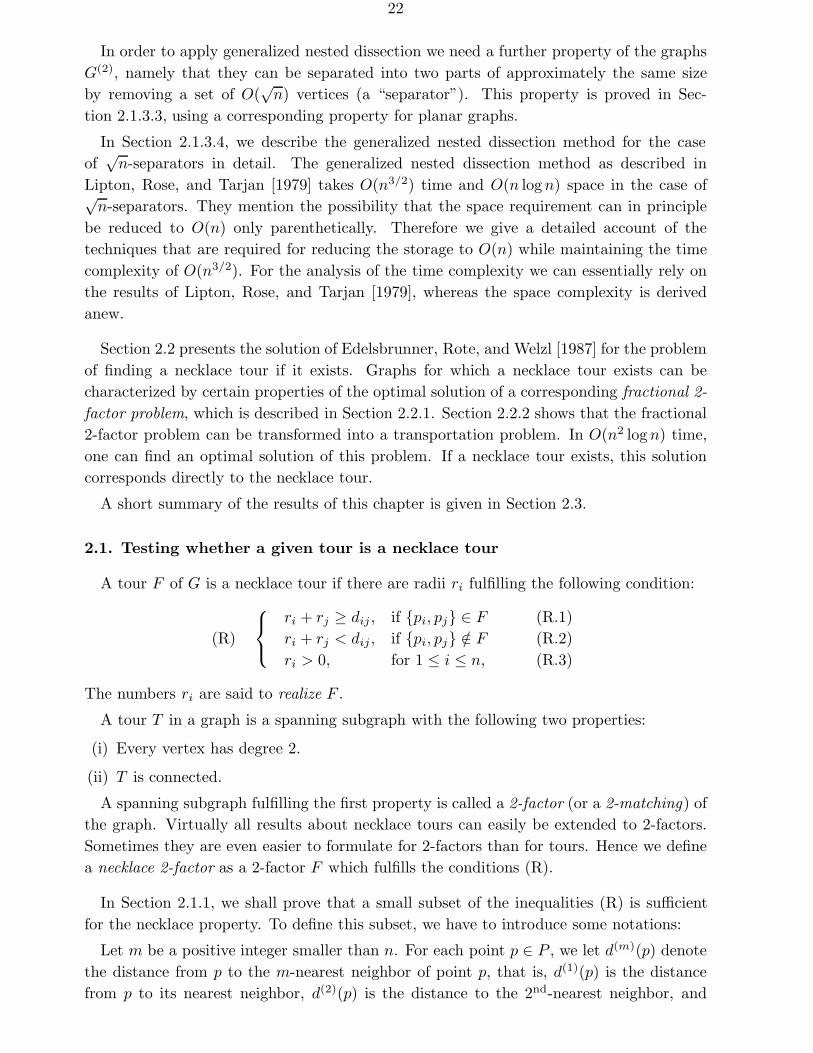
Figure 10. A set of disks D(2)(p) and the graph G(2)

so on. We define D(m)(p) to be the closed disk centered at p with radius d(m)(p). Thegraph G(m) is the intersection graph of these disks: There is an edge between two pointsif and only if the two disks intersect, i. e., if d(m)(pi) + d(m)(pj) ≥ dij . (cf. Figure 10).

In G(m), every vertex has at least degree m; therefore, the number of edges is at leastmn/2.

Theorem 9 in Section 2.1.1 says that the relations (R) have only to be checked for edgesin G(2). In Section 2.1.2, we shall prove that G(2) is a sparse graph, and we shall describehow G(2) can be constructed. Section 2.1.3 discusses the way how the reduced system canbe solved. The results are summarized in Section 2.3.

2.1.1. Systems of linear inequalities characterizing necklace tours

In this section we are going to prove that we can ignore the positivity constraints (R.3)and that we only need to check edges of G(2), i. e., we can replace (R.2) by

ri + rj < dij , if pi, pj ∈ G(2) \ F. (R.2′)

The proof is fairly technical and involved.

Theorem 9. Let F be a 2-factor. Then the following statements are equivalent:

(i) The system (R.1), (R.2), (R.3) is solvable (i. e., F is a necklace 2-factor).

(ii) The system (R.1), (R.2′) is solvable.

Proof: The non-trivial part is the conclusion from (ii) to (i). We proceed in several steps.

Lemma 10. Let ri be numbers fulfilling (R.1), (R.2′) for a 2-factor F . If ri ≤ 0, dij ≤ rj,

and dij ≤ d(2)(pj), then pi, pj ∈ F .

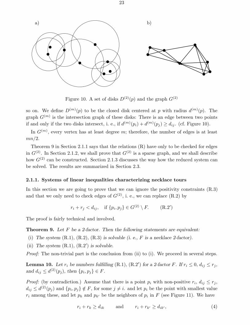
Proof: (by contradiction.) Assume that there is a point pi with non-positive ri, dij ≤ rj,dij ≤ d(2)(pj) and pi, pj /∈ F , for some j 6= i. and let pi be the point with smallest valueri among these, and let pk and pk′ be the neighbors of pi in F (see Figure 11). We have

ri + rk ≥ dik and ri + rk′ ≥ dik′ , (4)

24

pk′

pk

pj

pl

pi

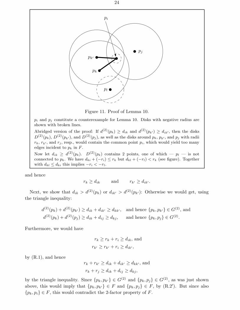
Figure 11. Proof of Lemma 10.

pi and pj constitute a counterexample for Lemma 10. Disks with negative radius areshown with broken lines.

Abridged version of the proof: If d(2)(pk) ≥ dik and d(2)(pk′) ≥ dik′ , then the disks

D(2)(pk), D(2)(pk′), and D(2)(pj), as well as the disks around pk, pk′ , and pj with radiirk, rk′ , and rj , resp., would contain the common point pi, which would yield too manyedges incident to pk in F .

Now let dik ≥ d(2)(pk). D(2)(pk) contains 2 points, one of which — pl — is notconnected to pk. We have dki + (−ri) ≤ rk but dkl + (−rl) < rk (see figure). Togetherwith dkl ≤ dki this implies −ri < −rl.

and hencerk ≥ dik and rk′ ≥ dik′ .

Next, we show that dik > d(2)(pk) or dik′ > d(2)(pk′): Otherwise we would get, usingthe triangle inequality:

d(2)(pk) + d(2)(pk′) ≥ dik + dik′ ≥ dkk′ , and hence pk, pk′ ∈ G(2), and

d(2)(pk) + d(2)(pj) ≥ dik + dij ≥ dkj , and hence pk, pj ∈ G(2).

Furthermore, we would have

rk ≥ rk + ri ≥ dik, and

rk′ ≥ rk′ + ri ≥ dik′ ,

by (R.1), and hencerk + rk′ ≥ dik + dik′ ≥ dkk′ , and

rk + rj ≥ dik + dij ≥ dkj ,

by the triangle inequality. Since pk, pk′ ∈ G(2) and pk, pj ∈ G(2), as was just shownabove, this would imply that pk, pk′ ∈ F and pk, pj ∈ F , by (R.2′). But since alsopk, pi ∈ F , this would contradict the 2-factor property of F .

25

Thus, we proved that at least one neighbor of pi (say, pk) fulfills

dik > d(2)(pk). (5)

There are at least two points pl with dkl ≤ d(2)(pk), by the definition of d(2)(pk). Notboth of them can be neighbors of k in F , since for one of the two neighbors of k, namelyi, we have dki > d(2)(pk). Hence there is a point pl with

dkl ≤ d(2)(pk) and pk, pl /∈ F. (6)

From that inequality follows pk, pl ∈ G(2) and hence, by (R.2′),

rk + rl < dkl.

From (4), (5), and (6), we getrl < ri ≤ 0,

and moreover we have also

dlk ≤ rk + rl ≤ rk, dlk ≤ d(2)(pk), and pk, pl /∈ F.

Thus, the point pl, together with pk, constitutes another counterexample to our lemma,contradicting the choice of pi as the counterexample with smallest ri at the beginning ofthe proof.

Lemma 11. If a set of values ri, i = 1, 2, . . . , n, fulfills (R.1) and (R.2′) then the values

r′i :=

d(2)(pi), if ri > d(2)(pi) ,0, if ri < 0 , andri, otherwise ,

also fulfill (R.1) and (R.2′).

Proof: We have now 0 ≤ r′i ≤ d(2)(pi), for all i. In the proof below, we distinguish twocases, namely the case that an edge belongs to F and the case that it belongs to G(2) \F .We treat the second case first.

(i) If pi, pj ∈ G(2) \ F , then we have ri + rj < dij . The corresponding inequality

r′i + r′j < dij

can be violated only if one previous variable (say, ri) is negative, which implies r′i = 0.In this case, rj ≥ dij would imply rj ≥ r′j ≥ dij and d(2)(pj) ≥ r′j ≥ dij , which wouldcontradict Lemma 10. Thus, we have

r′j < dij and r′i + r′j = r′j < dij .

(ii) If pi, pj ∈ F , then we have ri + rj ≥ dij . The corresponding inequality

r′i + r′j ≥ dij

26

can become violated only if one variable ri or rj (say, ri) is greater than d(2)(pi), whichimplies r′i = d(2)(pi). We have d(2)(pi) ≥ dik for at least 2 points pk. Hence,

r′i + r′k ≥ r′i = d(2)(pi) ≥ dik and

d(2)(pi) + d(2)(pk) ≥ d(2)(pi) ≥ dik,

which implies pi, pk ∈ G(2), for at least 2 points pk. We have pi, pk ∈ F , for each ofthese points, since, otherwise, r′i + r′k < dik, by part (i) of this proof. But there are only 2points pk with pi, pk ∈ F . Thus,

r′i + r′k ≥ dik

holds for all points pk with pi, pk ∈ F and therefore also for point pj .

Now, we come to the conclusion of the proof of Theorem 9. By the preceding lemma,we have transformed a solution of (R.1), (R.2′) into a solution fulfilling the additionalconstraints

0 ≤ ri ≤ d(2)(pi).

Now, for pi, pj /∈ G(2), we get the remaining inequalities of (R.2)

ri + rj ≤ d(2)(pi) + d(2)(pj) < dij

for free. Let δ = min dij − ri − rj | pi, pj /∈ F > 0. Then r′′i := ri + δ/3 still fulfillsall inequalities (R.1) and (R.2) and, in addition, we have r′′i > 0.

The following theorem is important because in the next section we will show that G(2)

of a set of points is a sparse graph.

Corollary 12. A realizable 2-factor F of a graph G is a subgraph of G(2).

Proof: Let r1, r2, . . ., rn be radii that realize F . According to the proof of Lemma 11,we can assume that they are positive and smaller than or equal to d(2)(p1), d(2)(p2), . . .,d(2)(pn). Therefore, each edge pi, pj belonging to F (we have ri + rj ≥ dij) also belongsto G(2) (because d(2)(pi) + d(2)(pj) ≥ dij).

27

2.1.2. Properties of the family of graphs G(2)

2.1.2.1. G(2) of a Set of Points in the Plane is Sparse

In the previous section we have shown that a necklace tour is a subgraph of G(2). Thissection shows that, for each natural number m, the graph G(m) of a set of n points in theplane has at most (19m − 1)n edges. In particular, G(2) has at most 37n edges.

We need the following lemma.

Lemma 13. (Reifenberg [1948], Bateman and Erdos [1951]) Let D0 be a disk in the plane,

and let S be a set of disks in the plane which are at least as big as D0, such that none of

their centers lies in the interior of D0 or of another disk in S. Then the number of disks

in S that intersect D0 is at most 18.

With this lemma, we can prove the main result of this section which guarantees thesparsity of G(m).

Theorem 14. Let P be a set of n points in the plane and let m be a natural number.

Then the edge set G(m) of the graph G(m) of P contains at most (19m − 1)n edges.

Proof: We claim that a smallest disk D0 in S(m) = D(m)(p) | p ∈ P intersects at most19m − 1 disks in S(m). From this the theorem follows by a simple inductive argument.

Let S be the set of disks in S(m) that intersect D0. We know that each disk in S containsat most m− 1 centers of other disks in its interior. We will now remove disks from S suchthat no center of a remaining disk lies in the interior of D0 or of any other remaining disk.This is done by the following procedure:

Step 1: Remove all disks from S that have their centers in the interior of D0.

Repeat the following step as long as there are disks in S which contain centers ofother disks of S in their interior:

Step 2: Choose the largest among these disks and remove all disks from S whosecenters belong to its interior.

Obviously, the final set S has the desired property and we conclude that it contains atmost 18 disks.

In Step 1, at most m−1 disks are removed from S, since there are at most m−1 centersof disks in the interior of D0. Whenever a disk is chosen in Step 2, that disk will notbe chosen again. Moreover, the special choice as the largest disk guarantees that it willnot be removed in a later step. Consequently, each disk which is chosen in Step 2 will beone of the disks which finally remain. It follows that Step 2 is repeated at most 18 times.Moreover, at most m − 1 disks are removed from S in each repetition. Summing the thenumber of disks that are removed at each step and that finally remain, we get the followingbound on the initial cardinality of the set S:

|S| ≤ m − 1 + 18(m − 1) + 18 = 19m − 1.

28

We conjecture that the worst-case configuration for the theorem consists of (approxi-mately) equal-size disks. This would mean that the true upper bound for

∣∣G(1)∣∣ is 9n

instead of 18n, since all edges can be counted twice in the above proof. (Each disk is thesmallest.) Consequently, we would obtain a bound of (10m − 1)n for

∣∣G(m)∣∣.

2.1.2.2. Construction of G(2) for Points in the Plane

G(2) can be constructed using standard techniques from computational geometry.

Theorem 15. The graph G(2) of a set P of n points in the plane can be computed in

O(n logn) time and O(n) space.

Proof: In order to compute G(2) in O(n logn) time and O(n) space, we first calculate thevalue d(2)(p) for each point p in P . For this purpose, we consider the 3rd-order Voronoidiagram of P (see Preparata and Shamos [1985]). This is a partition of the plane intoconvex polygonal regions, where each region is the locus of points of the plane whosethree nearest neighbors are some fixed three points. This partition can be constructedin O(n logn) time and O(n) space (see Lee [1982]). Next, we compute the 2nd-nearestneighbor of each of the n points in P in O(n logn) time. This is done by locating foreach point p of P the region of the diagram it lies in (for a solution to this point locationproblem, see Edelsbrunner, Guibas, and Stolfi [1986]). Then we determine which of thethree points given by the located region is furthest away from p. (One of the three pointsis p itself.) Thus, in O(n logn) time, we can determine the numbers d(2)(p), for all pointsp in P .

Next, we find all pairs p1, p2 of points in P whose corresponding disks intersect:

D(2)(p1) ∩ D(2)(p2) 6= ∅.

By construction, no disk is contained in the interior of another disk. Hence, D(2)(p1) ∩D(2)(p2) 6= ∅ if and only if the bounding circles intersect. We thus have the problem ofreporting all intersecting pairs of n circles. Using the plane-sweep technique of Bentleyand Ottmann [1979], this can be done in O(n logn + k log n) time, where k is the numberof reported pairs. By Theorem 14, k = O(n), and therefore the overall complexity isO(n logn). For all algorithms mentioned, O(n) space is sufficient which concludes theproof of the theorem.

29

2.1.3. Testing the system of inequalities for feasibility

Systems of linear inequalities have become a well-established area in mathematics (cf. themore specific remarks in Section 2.1.3.2). Linear programming, which is just the minimiza-tion of a linear function subject to a system of linear inequalities, is by now a classicalfield of applied mathematics, although it is still a very active area of research, and manystriking advances have been made only in the last few years.

In our case however, we do not want to optimize an objective function, we only wantto check feasibility (although these two problems are theoretically equivalent, in a certainsense). Furthermore, our systems of inequalities have a special structure: Only two vari-ables occur in each inequality, and the coefficients are ±1. This will allow us to applygraph-theoretic methods for these systems.

In Section 2.1.3.1 we will transform the system of inequalities characterizing necklacetours into an equivalent system where all inequalities are of the form

vj ≤ vi + cij , or

vj < vi + cij .

Although this is necessary neither theoretically nor from a practical viewpoint, it will allowus a simpler formulation of the algorithms in the subsequent sections.

Section 2.1.3.2 discusses two possible approaches for solving these systems from a generalpoint of view: the shortest path approach and the elimination approach.

A special class of elimination algorithms which are called generalized nested dissectionrequire that the graphs can be separated into two approximately equal parts by removinga small subset of the vertices (a separator). Section 2.1.3.3 defines this property exactlyand proves the separator theorem for our class of graphs. It is also shown how separatorscan be constructed.

Section 2.1.3.4 describes the generalized nested dissection method in detail. The con-clusions from all these results are summarized in Section 2.3.

30

2.1.3.1. Transformation of the inequalities

The inequalities of the system (R.1) and (R.2′), whose solvability we want to check, are ofthe following two forms:

(T)

ri + rj ≥ dij , if pi, pj ∈ F (R.1)ri + rj < dij , if pi, pj ∈ G(2) \ F. (R.2′)

These inequalities are not suited to be modeled by a directed graph; therefore we transformthem as follows: For the sake of symmetry, we first double the number of inequalities:

(T′)

−ri ≤ rj − dij , if pi, pj ∈ F

−rj ≤ ri − dij , if pi, pj ∈ F

ri < −rj + dij , if pi, pj ∈ G(2) \ F

rj < −ri + dij , if pi, pj ∈ G(2) \ F.

In order to set up our directed graph, it is advantageous to introduce a new variable ri foreach ri, where ri represents −ri.

Using the new variables, we rewrite system (T′) to

(T′′.1)

ri ≤ rj − dij , if pi, pj ∈ F

rj ≤ ri − dij , if pi, pj ∈ F

ri < rj + dij , if pi, pj ∈ G(2) \ F

rj < ri + dij , if pi, pj ∈ G(2) \ F.

With the additional constraints

(T′′.2) ri = −ri, for all i,

the system (T′′) consisting of the constraints (T′′.1) and (T′′.2) is equivalent to the system(T′) and therefore to the system (T).

Lemma 16. The system (T′′.1)-(T′′.2) has a solution if and only if the system (T′′.1) has

a solution.

Proof: The “only if” part is clear. If (r′i, r′i) is a solution of (T′′.1) then (ri, ri) with

ri = 12 (r′i − r′i), and ri = 1

2 (r′i − r′i),

is a solution of (T′′.1) and (T′′.2) as can be checked easily.

Hence, with respect to solvability, we can ignore the equations (T′′.2), and we only haveto consider inequalities of the form

vj ≤ vi + cij , and

vj < vi + cij ,

where the cij can be arbitrary (positive or negative) real numbers.

We remark that in general, the above transformation can be carried out for any systemwith at most two variables in each inequality and with coefficients ±1. It can even begeneralized to systems with arbitrary coefficients.

31

2.1.3.2. Graph-theoretic approaches to solving systems of inequalities

In the previous section, we have transformed the system of inequalities which we want tosolve into an equivalent system where all inequalities are of the form

vj ≤ vi + cij , and

vj < vi + cij .

For simplicity, let us first discuss systems with inequalities of the first form only:

vj ≤ vi + cij .

Let us draw a vertex for every variable vj and an arc from vi to vj of weight cij for everyinequality. We shall identify each variable with its corresponding vertex. Let us denotethe resulting weighted directed graph by G = (V, E, c).

It is well known that the solvability of the system of inequalities can be checked by asingle-source shortest path computation on this graph (cf. Rockafellar [1984], Chapter 6).If the graph contains no negative cycles, the shortest path problem can be solved, andthe shortest distances are a solution of the inequality system. If the graph contains anegative cycle, the system is unsolvable. This approach was followed in Edelsbrunner,Rote, and Welzl [1987]. The single-source shortest path problem in the presence of negativearc lengths can be solved by the Bellman-Ford algorithm in O(|V | |E|) time (see Lawler[1976]). Since |V | = O(n) and |E| = O(n) in our case, this leads to an O(n2) algorithmfor checking the system.

One only has to take special care of the strict inequalities: If the graph contains a cycleof zero length which contains an arc corresponding to a strict inequality, the system is alsoinfeasible. The checking of this additional condition and the modification of the shortestdistances to account for the strict inequalities are described in detail in Edelsbrunner,Rote, and Welzl [1987], Section 5.

On the other hand, we can use elimination procedures for solving systems of inequalitiesof the type considered. Although elimination schemes like Gaußian elimination or Gauß-Jordan elimination were first applied in numerical linear algebra and were hence originallydescribed in matrix terminology, they can be conveniently described in a graph-theoreticframework, which is also more appropriate in the context of our application.

Let us again consider the graph G = (V, E, c) corresponding to a system of weak in-equalities of the form

vj ≤ vi + cij .

The above system can be expressed as

max(j,k)∈E

(vk − cjk) ≤ vj ≤ min(i,j)∈E

(vi + cij), for all j.

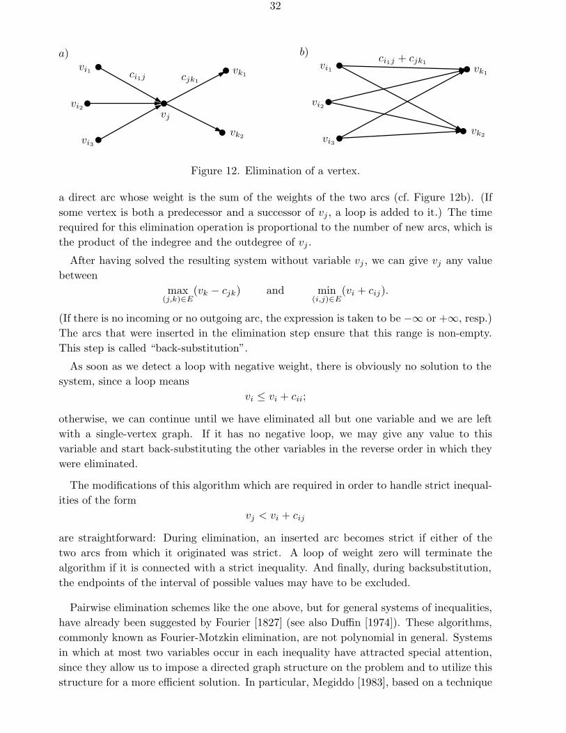
Let us look at all arcs that enter or leave a vertex vj (Figure 12a). We can eliminatethe variable vj and its incident arcs by inserting direct arcs from all its predecessors toall its successors. More specifically, for each pair of incoming and outgoing arcs, we add

32

vi1

vi2

vi3

vk1

vk2

vj

ci1j cjk1

a)vi1

vi2

vi3

vk1

vk2

ci1j + cjk1

b)

Figure 12. Elimination of a vertex.

a direct arc whose weight is the sum of the weights of the two arcs (cf. Figure 12b). (Ifsome vertex is both a predecessor and a successor of vj , a loop is added to it.) The timerequired for this elimination operation is proportional to the number of new arcs, which isthe product of the indegree and the outdegree of vj .

After having solved the resulting system without variable vj , we can give vj any valuebetween

max(j,k)∈E

(vk − cjk) and min(i,j)∈E

(vi + cij).

(If there is no incoming or no outgoing arc, the expression is taken to be −∞ or +∞, resp.)The arcs that were inserted in the elimination step ensure that this range is non-empty.This step is called “back-substitution”.

As soon as we detect a loop with negative weight, there is obviously no solution to thesystem, since a loop means

vi ≤ vi + cii;

otherwise, we can continue until we have eliminated all but one variable and we are leftwith a single-vertex graph. If it has no negative loop, we may give any value to thisvariable and start back-substituting the other variables in the reverse order in which theywere eliminated.

The modifications of this algorithm which are required in order to handle strict inequal-ities of the form

vj < vi + cij

are straightforward: During elimination, an inserted arc becomes strict if either of thetwo arcs from which it originated was strict. A loop of weight zero will terminate thealgorithm if it is connected with a strict inequality. And finally, during backsubstitution,the endpoints of the interval of possible values may have to be excluded.

Pairwise elimination schemes like the one above, but for general systems of inequalities,have already been suggested by Fourier [1827] (see also Duffin [1974]). These algorithms,commonly known as Fourier-Motzkin elimination, are not polynomial in general. Systemsin which at most two variables occur in each inequality have attracted special attention,since they allow us to impose a directed graph structure on the problem and to utilize thisstructure for a more efficient solution. In particular, Megiddo [1983], based on a technique

33

in Shostak [1981], gives an O(m·n3 log m) time algorithm to solve systems of m inequalitiesand n variables, where each inequality contains at most two variables.

The connection between algorithms for solving systems of linear equations and algo-rithms for certain graph problems has been known for some time (cf. e. g. Carre [1971]).In the meantime, a common algebraic foundation for both types of problems (and others)has been established (cf. Lehmann [1977], Carre [1979], Gondran and Minoux [1979], Zim-mermann [1981] Chapter 8). In order to formulate them in the proper algebraic settingone has to use a semiring. The linear algebra problems use the semiring (IR, +, ·), whichis even a ring, whereas the shortest path problems use the semiring (IR, max, +). Thealgorithm presented above corresponds to Gaußian elimination. Conventionally, the elimi-nation algorithms are described algebraically. In our application, we can directly describethe idea of vertex elimination using graph-theoretic terms.

Of course, the amount of work and storage space depends on the number of new arcswhich are inserted during the elimination process (the so-called “fill-in”), and this num-ber again depends on the elimination ordering. In the worst case, conventional Gaußianelimination (for dense matrices) takes O(n3) steps and O(n2) space. However, by usingthe special structure of the underlying graph, we can reduce the time to O(n3/2) and thespace to O(n), even without taking advantage of the property that all non-zero coefficientshave absolute value 1.

In the next section we will define the property that is required of the graphs, and we willshow that it holds for the graphs G(2) which are of interest to us. Afterwards we returnto the topic of vertex elimination algorithms, and we describe how the time complexityclaimed above can be achieved.

2.1.3.3.√

n-separators for G(2)

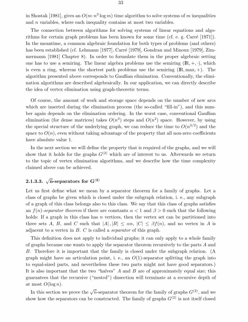
Let us first define what we mean by a separator theorem for a family of graphs. Let aclass of graphs be given which is closed under the subgraph relation, i. e., any subgraphof a graph of this class belongs also to this class. We say that this class of graphs satisfiesan f(n)-separator theorem if there are constants α < 1 and β > 0 such that the followingholds: If a graph in this class has n vertices, then the vertex set can be partitioned intothree sets A, B, and C such that |A| , |B| ≤ αn, |C| ≤ βf(n), and no vertex in A isadjacent to a vertex in B. C is called a separator of this graph.

This definition does not apply to individual graphs; it can only apply to a whole familyof graphs because one wants to apply the separator theorem recursively to the parts A andB. Therefore it is important that the family is closed under the subgraph relation. (Agraph might have an articulation point, i. e., an O(1)-separator splitting the graph intoto equal-sized parts, and nevertheless these two parts might not have good separators.)It is also important that the two “halves” A and B are of approximately equal size; thisguarantees that the recursive (“nested”) dissection will terminate at a recursive depth ofat most O(log n).

In this section we prove the√

n-separator theorem for the family of graphs G(2), and weshow how the separators can be constructed. The family of graphs G(2) is not itself closed

34

under the subgraph relation; therefore we have to mention their subgraphs explicitly whenwe formulate the theorem.

Our results are based on the corresponding results for planar graphs, and hence wecite these results first. They use a generalization of the concept of separators, where thevertices have weights, and the size of the parts A and B is measured by their total weights.(The size of the separator is still measured by its cardinality.)

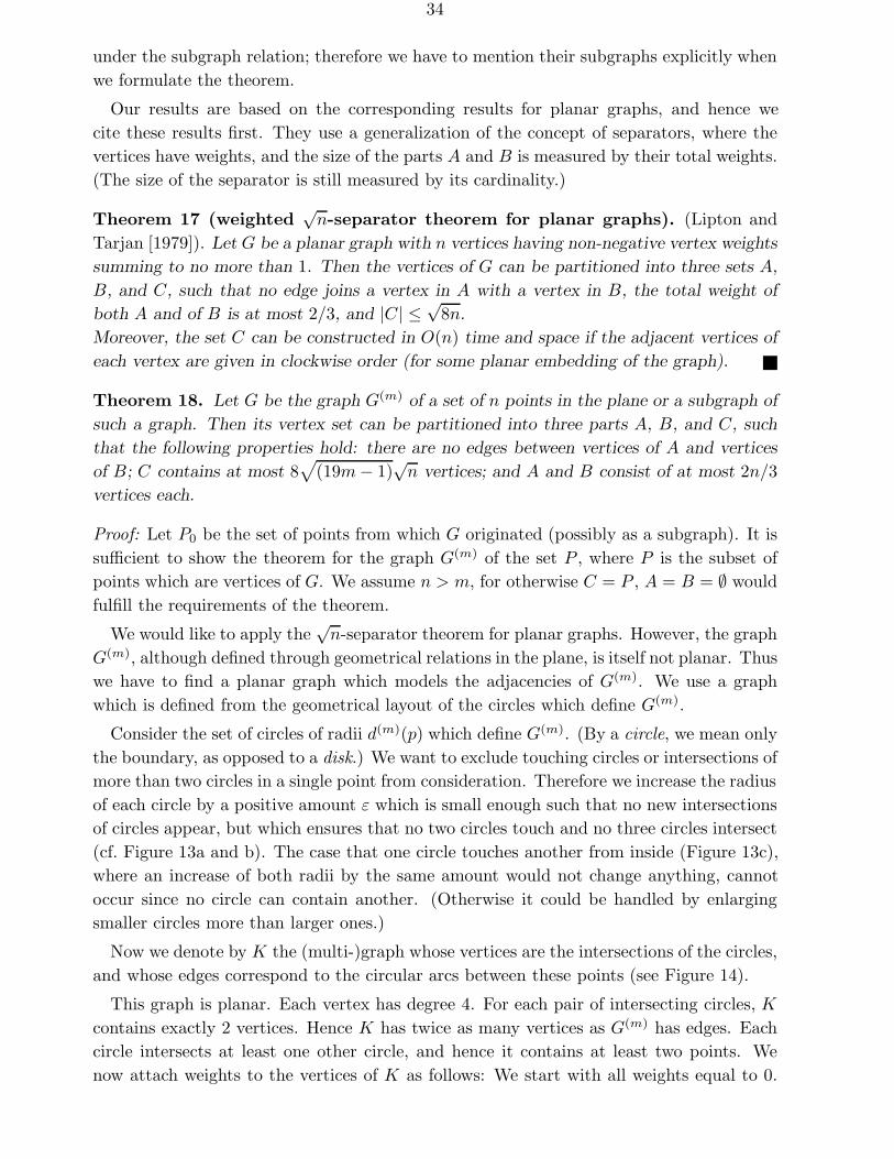
Theorem 17 (weighted√

n-separator theorem for planar graphs). (Lipton andTarjan [1979]). Let G be a planar graph with n vertices having non-negative vertex weights

summing to no more than 1. Then the vertices of G can be partitioned into three sets A,

B, and C, such that no edge joins a vertex in A with a vertex in B, the total weight of

both A and of B is at most 2/3, and |C| ≤ √8n.

Moreover, the set C can be constructed in O(n) time and space if the adjacent vertices of

each vertex are given in clockwise order (for some planar embedding of the graph).

Theorem 18. Let G be the graph G(m) of a set of n points in the plane or a subgraph of

such a graph. Then its vertex set can be partitioned into three parts A, B, and C, such

that the following properties hold: there are no edges between vertices of A and vertices

of B; C contains at most 8√

(19m − 1)√

n vertices; and A and B consist of at most 2n/3vertices each.

Proof: Let P0 be the set of points from which G originated (possibly as a subgraph). It issufficient to show the theorem for the graph G(m) of the set P , where P is the subset ofpoints which are vertices of G. We assume n > m, for otherwise C = P , A = B = ∅ wouldfulfill the requirements of the theorem.

We would like to apply the√

n-separator theorem for planar graphs. However, the graphG(m), although defined through geometrical relations in the plane, is itself not planar. Thuswe have to find a planar graph which models the adjacencies of G(m). We use a graphwhich is defined from the geometrical layout of the circles which define G(m).

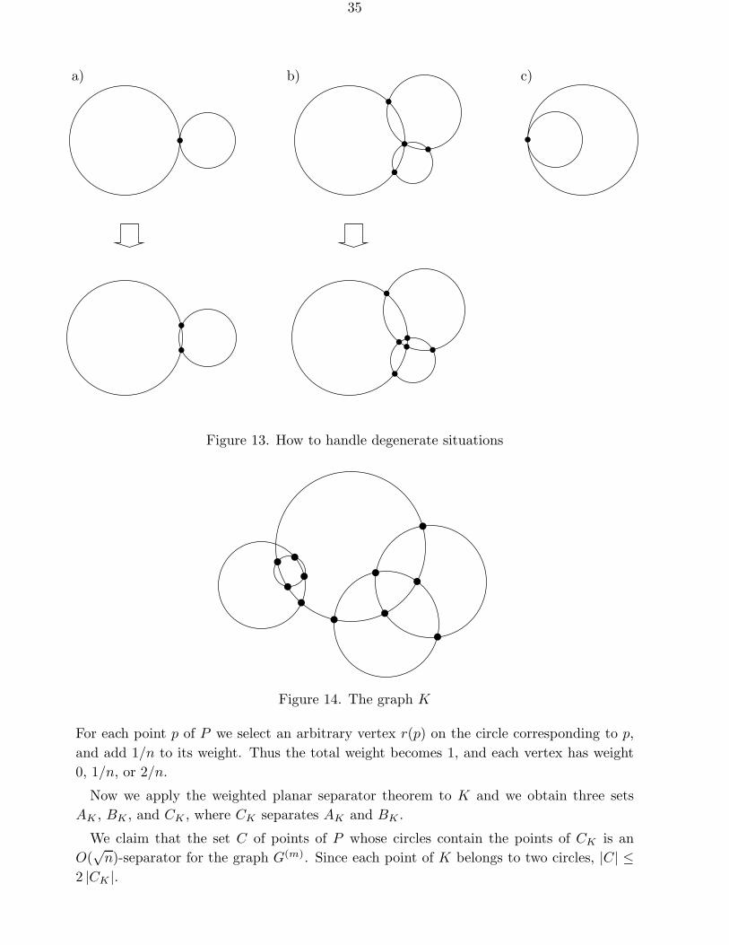
Consider the set of circles of radii d(m)(p) which define G(m). (By a circle, we mean onlythe boundary, as opposed to a disk.) We want to exclude touching circles or intersections ofmore than two circles in a single point from consideration. Therefore we increase the radiusof each circle by a positive amount ε which is small enough such that no new intersectionsof circles appear, but which ensures that no two circles touch and no three circles intersect(cf. Figure 13a and b). The case that one circle touches another from inside (Figure 13c),where an increase of both radii by the same amount would not change anything, cannotoccur since no circle can contain another. (Otherwise it could be handled by enlargingsmaller circles more than larger ones.)

Now we denote by K the (multi-)graph whose vertices are the intersections of the circles,and whose edges correspond to the circular arcs between these points (see Figure 14).

This graph is planar. Each vertex has degree 4. For each pair of intersecting circles, K

contains exactly 2 vertices. Hence K has twice as many vertices as G(m) has edges. Eachcircle intersects at least one other circle, and hence it contains at least two points. Wenow attach weights to the vertices of K as follows: We start with all weights equal to 0.

35

a) b) c)

Figure 13. How to handle degenerate situations

Figure 14. The graph K

For each point p of P we select an arbitrary vertex r(p) on the circle corresponding to p,and add 1/n to its weight. Thus the total weight becomes 1, and each vertex has weight0, 1/n, or 2/n.

Now we apply the weighted planar separator theorem to K and we obtain three setsAK , BK , and CK , where CK separates AK and BK .

We claim that the set C of points of P whose circles contain the points of CK is anO(

√n)-separator for the graph G(m). Since each point of K belongs to two circles, |C| ≤

2 |CK |.

36

The sets A and B are defined as the sets of points p of P which do not belong to C andwhose representative points r(p) belong to AK and BK , resp.

We have to prove that G(m) contains no edge between A and B. If two points p and q ofP are connected by an edge in G(m) then the two circles corresponding to p and q intersect.The two vertices r(p) and r(q) which carry the weights of p and q must be connected bya path in K which uses only edges which are pieces of the two circles.

If neither p not q belongs to C then this path must still exist in the graph K \ CK .Hence r(p) and r(q) belong to the same component of K \ CK , i. e., they belong eitherboth to AK or both to BK . Concluding, we have proved that if neither p nor q belongs toC, then they belong both to A or both to B.

We still have to prove the claimed bounds on the cardinalities of A, B, and C. AK

and BK have weight at most 2/3, hence A and B contain at most 2n/3 points. CK

contains at most√

8√|V (K)| =

√8√

2∣∣G(m)

∣∣ vertices. Since∣∣G(m)

∣∣ ≤ (19m − 1)n, we

have |CK | ≤√16(19m− 1)n, and hence |C| ≤ 2 |CK | ≤ 8√

(19m − 1)n.

Corollary 19. The family of the graphs G(2) and their subgraphs satisfies a√

n-separator

theorem with α = 2/3 and β = 8√

37.

Finally, we address the question how the separator for a graph G(2) can be found quickly.It is clear from the proof of the preceding theorem that if the graph K is available, the restof the construction needs only linear time: Since each vertex of K has only degree 4, therequirement of Theorem 17 that the neighbors are given in sorted order can be triviallyfulfilled in linear time.

The following theorem shows that, for a given graph G(2), K can be constructed inO(n logn) time. In Section 2.1.4., where separators have to be found repeatedly for dif-ferent subgraphs of G(2), we will build the graphs K for these subgraphs as kind of “sub-graphs” of the graph K of the original graph G(2). It will turn out that in the context ofthat application each individual separator construction takes only linear time.

Lemma 20. The graph K of the previous theorem can be constructed in O(n logn) time,

along with the construction of G(2).

We refer to the construction of G(2) according to Theorem 15. There, all intersections ofcircles were computed. These intersections form the vertex set of K, and the edges of K,which are arcs of the circles, are readily available during the plane-sweep. It only remainsto discuss how the degeneracies, namely two circles which touch, and three of more circleswhich intersect in a common point, should be treated. Touching circles can be handledby simply generating two vertices instead of one. If three or more circles intersect in onepoint, the plane-sweep algorithm will notice this as two intersections which have the samecoordinates. Since it processes the intersections according to the value of one coordinate,this means that there is a tie in deciding which intersection to process next. The algorithmcan break this tie by implicitly applying the trick of enlarging the circles by a small amountε, as in the proof of the previous theorem. In this way, the intersections, which are actuallyone point, will appear as different intersections, and they will yield different vertices of thegraph K.

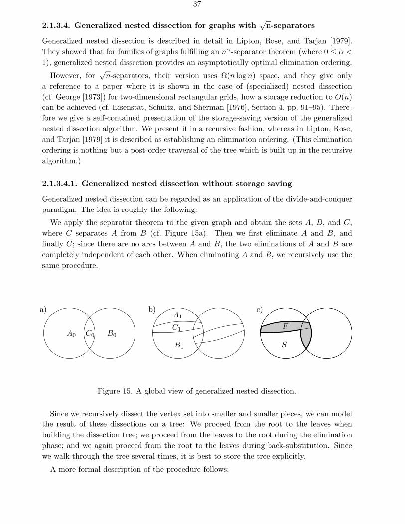
37

2.1.3.4. Generalized nested dissection for graphs with√

n-separators

Generalized nested dissection is described in detail in Lipton, Rose, and Tarjan [1979].They showed that for families of graphs fulfilling an nα-separator theorem (where 0 ≤ α <

1), generalized nested dissection provides an asymptotically optimal elimination ordering.

However, for√

n-separators, their version uses Ω(n log n) space, and they give onlya reference to a paper where it is shown in the case of (specialized) nested dissection(cf. George [1973]) for two-dimensional rectangular grids, how a storage reduction to O(n)can be achieved (cf. Eisenstat, Schultz, and Sherman [1976], Section 4, pp. 91–95). There-fore we give a self-contained presentation of the storage-saving version of the generalizednested dissection algorithm. We present it in a recursive fashion, whereas in Lipton, Rose,and Tarjan [1979] it is described as establishing an elimination ordering. (This eliminationordering is nothing but a post-order traversal of the tree which is built up in the recursivealgorithm.)

2.1.3.4.1. Generalized nested dissection without storage saving

Generalized nested dissection can be regarded as an application of the divide-and-conquerparadigm. The idea is roughly the following:

We apply the separator theorem to the given graph and obtain the sets A, B, and C,where C separates A from B (cf. Figure 15a). Then we first eliminate A and B, andfinally C; since there are no arcs between A and B, the two eliminations of A and B arecompletely independent of each other. When eliminating A and B, we recursively use thesame procedure.

C0 B0A0

a)

C1

B1

A1b) c)

F

S

Figure 15. A global view of generalized nested dissection.

Since we recursively dissect the vertex set into smaller and smaller pieces, we can modelthe result of these dissections on a tree: We proceed from the root to the leaves whenbuilding the dissection tree; we proceed from the leaves to the root during the eliminationphase; and we again proceed from the root to the leaves during back-substitution. Sincewe walk through the tree several times, it is best to store the tree explicitly.

A more formal description of the procedure follows:

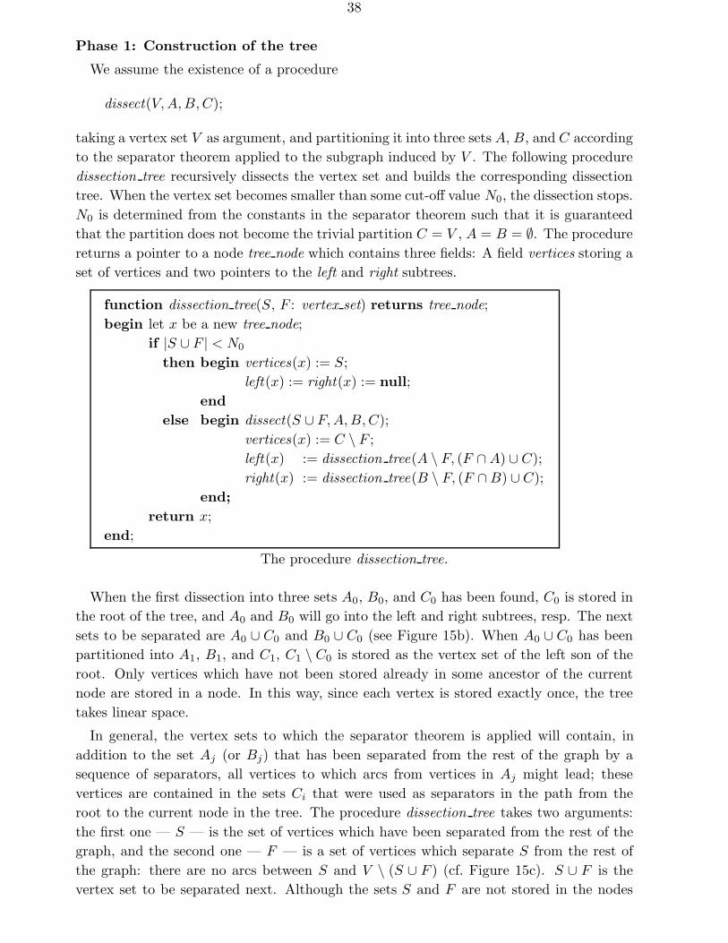
38

Phase 1: Construction of the tree

We assume the existence of a procedure

dissect(V, A, B, C);

taking a vertex set V as argument, and partitioning it into three sets A, B, and C accordingto the separator theorem applied to the subgraph induced by V . The following proceduredissection tree recursively dissects the vertex set and builds the corresponding dissectiontree. When the vertex set becomes smaller than some cut-off value N0, the dissection stops.N0 is determined from the constants in the separator theorem such that it is guaranteedthat the partition does not become the trivial partition C = V , A = B = ∅. The procedurereturns a pointer to a node tree node which contains three fields: A field vertices storing aset of vertices and two pointers to the left and right subtrees.

function dissection tree(S, F : vertex set) returns tree node;begin let x be a new tree node;

if |S ∪ F | < N0

then begin vertices(x) := S;left(x) := right(x) := null;

endelse begin dissect(S ∪ F, A, B, C);

vertices(x) := C \ F ;left(x) := dissection tree(A \ F, (F ∩ A) ∪ C);right(x) := dissection tree(B \ F, (F ∩ B) ∪ C);

end;return x;

end;

The procedure dissection tree.

When the first dissection into three sets A0, B0, and C0 has been found, C0 is stored inthe root of the tree, and A0 and B0 will go into the left and right subtrees, resp. The nextsets to be separated are A0 ∪ C0 and B0 ∪ C0 (see Figure 15b). When A0 ∪ C0 has beenpartitioned into A1, B1, and C1, C1 \ C0 is stored as the vertex set of the left son of theroot. Only vertices which have not been stored already in some ancestor of the currentnode are stored in a node. In this way, since each vertex is stored exactly once, the treetakes linear space.

In general, the vertex sets to which the separator theorem is applied will contain, inaddition to the set Aj (or Bj) that has been separated from the rest of the graph by asequence of separators, all vertices to which arcs from vertices in Aj might lead; thesevertices are contained in the sets Ci that were used as separators in the path from theroot to the current node in the tree. The procedure dissection tree takes two arguments:the first one — S — is the set of vertices which have been separated from the rest of thegraph, and the second one — F — is a set of vertices which separate S from the rest ofthe graph: there are no arcs between S and V \ (S ∪ F ) (cf. Figure 15c). S ∪ F is thevertex set to be separated next. Although the sets S and F are not stored in the nodes

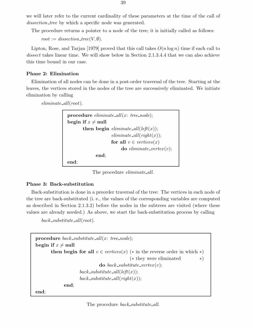
39

we will later refer to the current cardinality of these parameters at the time of the call ofdissection tree by which a specific node was generated.

The procedure returns a pointer to a node of the tree; it is initially called as follows:

root := dissection tree(V, ∅).Lipton, Rose, and Tarjan [1979] proved that this call takes O(n logn) time if each call to

dissect takes linear time. We will show below in Section 2.1.3.4.4 that we can also achievethis time bound in our case.

Phase 2: Elimination

Elimination of all nodes can be done in a post-order traversal of the tree. Starting at theleaves, the vertices stored in the nodes of the tree are successively eliminated. We initiateelimination by calling

eliminate all(root).

procedure eliminate all(x: tree node);begin if x 6= null

then begin eliminate all(left(x));eliminate all(right(x));for all v ∈ vertices(x)

do eliminate vertex (v);end;

end;

The procedure eliminate all.

Phase 3: Back-substitution

Back-substitution is done in a preorder traversal of the tree: The vertices in each node ofthe tree are back-substituted (i. e., the values of the corresponding variables are computedas described in Section 2.1.3.2) before the nodes in the subtrees are visited (where thesevalues are already needed.) As above, we start the back-substitution process by calling

back substitute all(root).

procedure back substitute all(x: tree node);begin if x 6= null

then begin for all v ∈ vertices(x) (∗ in the reverse order in which ∗)(∗ they were eliminated ∗)

do back substitute vertex (v);back substitute all(left(x));back substitute all(right(x));

end;end;

The procedure back substitute all.

40

2.1.3.4.2. Analysis of the fill-in

Let us analyze the number of arcs that are inserted by the elimination. First, an insertedarc that starts in a vertex stored in some node of the tree can only go to a vertex stored inthe same node or in an ancestor or a descendant of this node; there can be no “cross arcs”relative to the tree: When eliminate all(x) is called for some node x, there are initially noarcs between the vertices stored in the subtree left(x) and the vertices stored in the subtreeright(x). When eliminating these vertices, new arcs are inserted only between vertices thatare adjacent to the same node, i. e., between pairs of vertices which are both stored inleft(x) or in right(x), or between such vertices and vertices stored in x.

In the following treatment we closely follow the analysis given in Lipton, Rose, andTarjan [1979].

For estimating the number of inserted arcs, we first count the number of arcs betweenvertices stored in the same node x. If x was built in a call to dissection tree with parametersS and F and the dissection of S ∪ F was A ∪ B ∪ C, then |C| is an upper bound on thenumber of vertices stored in x, and hence |C|2 is an upper bound on the number of arcsbetween vertices stored in x.

Now let us count the number of arcs that run between a vertex stored in x and a vertexstored in an ancestor of x (in either direction). F is the set of vertices stored in ancestorsof x to which the vertices stored in x (and in the whole subtree rooted at x, i. e., thevertices in S) can possibly be adjacent. Thus, 2 |C| |F | is an upper bound on the numberof these arcs.

In the following, we derive an upper bound f(n, l) on the number of inserted arcs whichare incident to vertices stored in the subtree rooted at a node x which was created with|S ∪ F | = n, |F | = l and |C| = c. We have

f(n, l) = c2 + 2cl (for the vertices in x)+ max

n1,n2,l1,l2(f(n1, l1) + f(n2, l2)) (for the vertices in the subtrees) (7)

Let us find out over which values the maximum in this expression has to be taken: n1, l1and n2, l2 are the values of |S ∪ F | and |F | for the calls to dissection tree for left(x) andright(x), resp., i. e.,

n1 = |A ∪ C|n2 = |B ∪ C|

and

and

l1 = |(F ∩ A) ∪ C| ,l2 = |(F ∩ B) ∪ C| .

We haven1 = |A ∪ C| ≤ |A| + |C| ≤ 2n/3 + c, and

n1 = |A ∪ C| = |A ∪ B ∪ C| − |B| ≥ n − 2n/3 = n/3,

and analogous inequalities for n2; thus,

n/3 ≤ n1, n2 ≤ 2n/3 + c.

Moreover,

n1 + n2 = |A ∪ C| + |B ∪ C| = |A ∪ B ∪ C| + |C| = n + c, and

l1 + l2 = |(F ∩ A) ∪ C| + |(F ∩ B) ∪ C|≤ |F ∩ A| + |C| + |F ∩ B| + |C| ≤ |F | + 2 |C| = l + 2c.

41

By our separator theorem (Corollary 19), we have c ≤ β√

n, and we can write

f(n, l) =

n2, for n ≤ N0,

β2n + 2βl√

n + maxn/3≤n1,n2≤2n/3+β

√n

n1+n2≤n+β√

nl1+l2≤l+2β

√n

(f(n1, l1) + f(n2, l2)) , for n > N0.

By observing that f(n, l) is increasing in l, we can get a lower bound for f(n, l) if wereplace l by 0 on the right side and set n1 = n2 = n/2:

f(n, 0) ≥ β2n + 2f(n/2, 0).

From this recursion follows easily that f(n, 0), the upper bound for the total number ofinserted arcs in the algorithm, is Ω(n log n). (It is also known that the number of insertedarcs can really become as large as Ω(n logn). Lipton, Rose, and Tarjan [1979] show thatthe maximum number is actually Θ(n log n).)

2.1.3.4.3. Reducing the storage requirement

How can this superlinear space requirement be reduced? From the above recursion we seethat we must reduce the factor 2 on the right side; i. e., instead of needing the storage fortwo subproblems of approximately half the size we must require only the storage for one so-lution. This can be done by freeing the storage used by the first call to eliminate all(left(x))before the second call eliminate all(right(x)), i. e., globally speaking, by selectively for-getting and recomputing arcs. This will increase the computation time by only a constantfactor.

Let us discuss the required modifications in detail. Assume that after returning fromthe call to eliminate all(x) all arcs incident to vertices stored in x are deleted. Then, aftercalling eliminate all(left(root)) and eliminate all(right(root)), we could still eliminate thevariables in vertex (root) and back-substitute them. However, we could not compute thevalues of the other variables, since the necessary arcs were deleted. We have to repeat theelimination process, first for left(root), then for right(root). However, this time we now donot throw away the arcs incident to vertex (left(root)), but we use them to back-substitutetheir values.

Thus, there are now two versions of eliminate all : one with deletion, and one withbacksubstitution; both are variations of the original procedure.

The whole computation is started by calling

eliminate back substitute(root).

It can be proved by induction that

(i) after the procedure eliminate delete(x) or eliminate back substitute(x) returns to thecaller the graph is restored to its original status before the procedure was called;

(ii) when either eliminate delete(x) or eliminate back substitute(x) is being called, theonly inserted arcs run between vertices that are stored in nodes on the path from theroot to x.

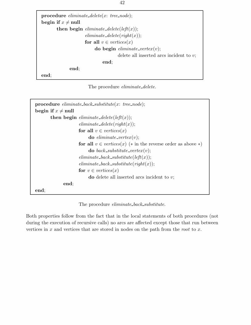
42

procedure eliminate delete(x: tree node);begin if x 6= null

then begin eliminate delete(left(x));eliminate delete(right(x));for all v ∈ vertices(x)

do begin eliminate vertex (v);delete all inserted arcs incident to v;

end;end;

end;

The procedure eliminate delete.

procedure eliminate back substitute(x: tree node);begin if x 6= null

then begin eliminate delete(left(x));eliminate delete(right(x));for all v ∈ vertices(x)

do eliminate vertex (v);for all v ∈ vertices(x) (∗ in the reverse order as above ∗)

do back substitute vertex (v);eliminate back substitute(left(x));eliminate back substitute(right(x));for v ∈ vertices(x)

do delete all inserted arcs incident to v;end;

end;

The procedure eliminate back substitute.

Both properties follow from the fact that in the local statements of both procedures (notduring the execution of recursive calls) no arcs are affected except those that run betweenvertices in x and vertices that are stored in nodes on the path from the root to x.

43

2.1.3.4.4. Performance analysis of the complete algorithm

Let us now analyze the storage requirement and the computation time required by themodified procedure.

We define f(n, l) to be an upper bound on the storage space needed for either elimi-nate delete or eliminate back substitute, where the same conventions hold with respect tothe meaning of n and l as with f(n, l).

The recursion for f(n, l) is also similar to the recursion (7) for f(n, l), except that thesum of the requirements for the two subproblems has to be replaced by their maximum,by property (i) above:

f(n, l) =

n2, for n ≤ N0,

β2n + 2βl√

n + maxn/3≤n1,n2≤2n/3+β

√n

n1+n2≤n+β√

nl1+l2≤l+2β

√n

max

f(n1, l1), f(n2, l2)

, for n > N0.

Since f(n, l) is isotone in both n and l, we can simplify this expression:

f(n, l) ≤ β2n + 2βl√

n + f(2n/3 + β√

n, l + 2β√

n), for n > N0.

We shall prove that f(n) = O(n).

Let N1 ≥ N0 be a number such that

2n/3 + β√

n ≤ 3n/4, for n > N1.

Then we can write

f(n, l) ≤

n2, for n ≤ N1,

β2n + 2βl√

n + f(3n/4, l + 2β√

n), for n > N1.

Denoting the additive term in the recursion by

h(n, l) = β2n + 2βl√

n

and expanding the recursion, we get

f(n, 0) ≤ h(n, 0) + h(n1, l1) + h(n2, l2) + · · · + N21 ,

whereni+1 = (3/4)ni = n (3/4)i and li+1 = li + β

√ni, l0 = 0.

We getli = 0 + β

√n + β

√n1 + · · ·β√ni−1

≤ β√

n(1 +

√3/4 +

√3/4

2+√

3/43+ · · ·

)= βγ

√n,

(8)

44

with γ = 1/(1 −√3/4) = 7.4641. Thus,

f(n, 0) ≤ N21 +

∞∑i=0

(β2ni + 2βli

√ni

)

≤ N21 +

∞∑i=0

(β2ni + 2β2γni

)

= N21 + β2(1 + 2γ)n

∞∑i=0

(3/4)i

= N21 + 4β2(1 + 2γ)n = O(n).

Thus we have proved:

Theorem 21. The elimination step in the modified algorithm takes O(n) space.

Remark: Actually, we have only proved that the amount of fill-in that has to be stored isO(n). The theorem is further supported by the implementational details which are givenin the next subsection.

Let us now analyze the running time of our algorithm. For the time complexity ofeliminate delete, as well as of eliminate all , we can set up a recursion as follows: Theamount of work for the elimination of a single vertex is proportional to the product of theindegree and the outdegree of this vertex. In a call to any of the elimination procedures, theindegree and the outdegree are bounded by c + l, where c and l have the same meaning asin Section 2.1.3.4.2. Since c vertices are eliminated, the time spent inside the subroutine,exclusive of the recursive calls, is O(c(c + l)2). Hence the total time requirement foreliminate delete or for eliminate all , which we denote by g(n, l), satisfies the followingrecursion

g(n, l) = c(c + l)2 + maxn1,n2,l1,l2

(g(n1, l1) + g(n2, l2))

≤ β√

n(β√

n + l)2 + maxn1,n2,l1,l2

(g(n1, l1) + g(n2, l2))

= O(√

n(√

n + l)2) + maxn1,n2,l1,l2

(g(n1, l1) + g(n2, l2)) ,

where the maximum has to be taken over the same range as for the recursion (7) inSection 2.1.3.4.2, and suitable initial conditions for n ≤ N0 have to be provided. Lipton,Rose, and Tarjan [1979] (p. 350–351, proof of Theorem 3) have shown that this recursionhas the solution

g(n, l) = O(√

n(√

n + l)2),

and henceg(n, 0) = O(n3/2).

Now let us denote by g(n, l) the time for the procedure eliminate back substitute. Therecursion for g(n, l) is similar to the above recursion for g(n, l), except that we have to add2g(n, l) on the right side for the two calls to eliminate delete. (The time for backsubsti-tution of a vertex is only the sum of the indegree and the outdegree of the vertex, hence

45

it is certainly dominated by the time for elimation and can be ignored in the asymptoticcomplexity.)

g(n, l) = c(c + l)2 + 2g(n, l) + maxn1,n2,l1,l2

(g(n1, l1) + g(n2, l2))

= O(√

n(√

n + l)2) + 2g(n, l) + maxn1,n2,l1,l2

(g(n1, l1) + g(n2, l2)) ,

However, it was shown above that g(n, l) = O(√

n(√

n+l)2). The term 2g(n, l) can thereforebe subsumed under the O-expression, and we get essentially the same recursion as above,only with a different constant:

g(n, l) = O(√

n(√

n + l)2) + maxn1,n2,l1,l2

(g(n1, l1) + g(n2, l2)) .

From this we conclude as above:

g(n, 0) = O(n3/2).

Thus we have proved:

Theorem 22. The elimination step in the modified algorithm takes O(n3/2) time.

The only part of the generalized nested dissection algorithm that has not been analyzedyet is the construction of the dissection tree. We will show that both the work and thestorage at the local level of a call to dissection tree with |S ∪ F | = n are O(n).

We assume that at the initial level we are given the graphs G(2) and K. Then the sepa-rator C can be constructed in linear time, as follows from the discussion in Section 2.1.3.3.The only problem is to ensure that the appropriate subgraphs of G(2) and the correspond-ing graphs K are available for the recursive calls, such that during these calls the separatorscan also be found in linear time. In other words, we are given a subgraph of G(2) inducedby the vertex set S ∪ F and the corresponding graph K; after finding the separator C

and the sets A and B, we have to construct the graph induced by A ∪ C and the graphK corresponding to it before the first recursive call, and similarly for the second recursivecall.

It is straightforward to remove all edges incident to B in order to obtain the subgraphof G(2) induced by A∪C. We update the graph K as follows: For each point of B, a wholecircle of the graph K must disappear. For each circle, we go through the vertices on thatcircle one by one. Each vertex which is encountered lies on two circles: the circle which isabout to disappear, and another circle. When the vertex is removed, its neighbors on thisother circle become adjacent, and the graph K must be updated to reflect this change. Itis clear that this can be done in time proportional to the size of the graph which is O(n).

Before the change, we make a local copy of both graphs that we deal with; so we do nothave to worry about restoring them for the second recursive call. Thus we need O(n) timeand space locally for each call. This leads to the following recursions for the total timeh(n, l) and the total space q(n, l) required by the procedure dissection tree:

h(n, l) = O(n) + maxn/3≤n1,n2≤2n/3+β

√n

n1+n2≤n+β√

nl1+l2≤l+2β

√n

(h(n1, l1) + h(n2, l2)), for n > N0,

46

andq(n, l) = O(n) + max

n/3≤n1,n2≤2n/3+β√

nn1+n2≤n+β

√n

l1+l2≤l+2β√

n

max q(n1, l1), q(n2, l2) , for n > N0.

For the time complexity h(n, l) we can refer to Theorem 2 of Lipton, Rose, and Tarjan[1979], where

h(n, 0) = O(n logn)

is obtained.

For q(n, l) we use the same trick as for the derivation of f(n, l), and we obtain

q(n, l) = O(n) + q(3n/4, l + 2β√

n), for n > N1.

We can proceed in the same way as for f(n, l) and we get

q(n, 0) = O(n).

Summarizing, we have

Theorem 23. The dissection tree can be built in O(n logn) time and O(n) space.

2.1.3.4.5. Details about the implementation

Since we talk about forgetting (i. e., deleting) arcs, we have to become specific about theway in which the graph is stored.

As we are dealing with sparse graphs, an adjacency list representation will probably beappropriate. However, during elimination, arcs may be inserted which are already in thegraph. We could replace duplicated arcs by a single arc whose weight is the smaller of thetwo weights. However, this creates the problem of detecting arc duplications quickly inadjacency lists. We could also leave multiple arcs in the adjacency lists. The eliminationalgorithm is insensitive to multiple arcs, except for the storage and processing time theyrequire: They cause no harm in the adjacency lists, and the algorithm will process twoarcs with equal endpoints without notice. However, the analysis of the algorithm, whichwas given above, makes the assumption that from a vertex set of cardinality a to a vertexset of cardinality b there are at most ab arcs. Therefore, the inserted arcs would not betaken into account correctly, if this scheme were used.

Therefore, we have to switch to an adjacency matrix representation, at least for parts ofthe graph. Because of the space requirements, the matrix representation is certainly notsuited for the original graph. Thus we must deal with two different representations in thesame algorithm: an adjacency list for the graph as it is originally given, and a dynamicalmatrix representation for the inserted arcs:

The vertices on the path from the root to the current node in the tree are pushed ona stack, and they are associated with the rows and columns of the adjacency matrix inthe order in which they appear on the stack. When the algorithm enters a new node,the corresponding number of rows and columns have to be added to the right and at the

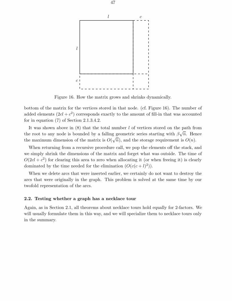
47

l

l c

c

Figure 16. How the matrix grows and shrinks dynamically.

bottom of the matrix for the vertices stored in that node. (cf. Figure 16). The number ofadded elements (2cl + c2) corresponds exactly to the amount of fill-in that was accountedfor in equation (7) of Section 2.1.3.4.2.

It was shown above in (8) that the total number l of vertices stored on the path fromthe root to any node is bounded by a falling geometric series starting with β

√n. Hence

the maximum dimension of the matrix is O(√

n), and the storage requirement is O(n).

When returning from a recursive procedure call, we pop the elements off the stack, andwe simply shrink the dimensions of the matrix and forget what was outside. The time ofO(2cl + c2) for clearing this area to zero when allocating it (or when freeing it) is clearlydominated by the time needed for the elimination (O(c(c + l)2)).

When we delete arcs that were inserted earlier, we certainly do not want to destroy thearcs that were originally in the graph. This problem is solved at the same time by ourtwofold representation of the arcs.

2.2. Testing whether a graph has a necklace tour

Again, as in Section 2.1, all theorems about necklace tours hold equally for 2-factors. Wewill usually formulate them in this way, and we will specialize them to necklace tours onlyin the summary.

48

2.2.1. Characterization of graphs which have necklace tours

To state our characterization, we formulate the optimal 2-factor problem as an integerprogram. Let G = (P, G) be a weighted graph with P = p1, p2, . . . , pn. We define abinary variable xij for each edge pi, pj of the graph, where xij = 1, if pi, pj belongs tothe 2-factor, and xij = 0, if it does not. The 2-factor problem can now be formulated asfollows:

(F)

minimize∑

pi,pj∈G

xijdij (F.1)

subject to∑

pi,pj∈G

xij = 2, for i = 1, 2, . . . , n, and (F.2)

xij ∈ 0, 1, for pi, pj ∈ G (F.3)

The linear programming relaxation of this problem, called the fractional 2-factor problem(FF) is obtained by replacing the constraints (F.3) by

0 ≤ xij ≤ 1, for pi, pj ∈ G. (FF.3)

Theorem 24. A graph G has a necklace 2-factor F if and only if the fractional 2-factor

problem defined by (F.1), (F.2), and (FF.3) has a unique optimal solution which is integral.

F is then the 2-factor corresponding to this solution.

Proof: (i) First we prove the “only if” part. Let r1, r2, . . . , rn be radii that realize F , thatis, they fulfill (R). Then it is clear that these radii can be made to fulfill

ri + rj > dij , if pi, pj ∈ F, and (R.1′)

ri + rj < dij , if pi, pj /∈ F, (R.2)

for example by adding δ/3 to all radii, where δ = min dij − ri − rj | pi, pj /∈ F > 0.Now assume that r1, r2, . . . , rn fulfill (R.1′) and (R.2). If we replace the distances dij inthe objective function (F.1) by d′

ij := dij − ri − rj , then we get∑pi,pj∈G

xijd′ij =

∑pi,pj∈G

xij(dij − ri − rj) =∑

pi,pj∈G

xijdij −∑

pi,pj∈G

xijri −∑

pi,pj∈G

xijrj

=∑

pi,pj∈G

xijdij −n∑

i=1

∑pi,pj∈G

xijri =∑

pi,pj∈G

xijdij −n∑

i=1

2ri,

by (F.2). Thus, the new objective function

(F.1′) minimize∑

pi,pj∈G

xijd′ij

differs from the old one by an additive constant, and the optimal solutions are the samewith respect to both objective functions. But we have

d′ij = dij − ri − rj < 0, for pi, pj ∈ F, and

d′ij = dij − ri − rj > 0, for pi, pj /∈ F.

49

Therefore, the unique optimal solution of (F.1′) subject to (FF.3) is the solution corre-sponding to F :

xij = 1, for d′ij < 0 (pi, pj ∈ F ), and

xij = 0, for d′ij > 0 (pi, pj /∈ F ),

and this solution also fulfills (F.2) and is thus the unique optimal solution of (F.1) subjectto (F.2), and (FF.3).

(ii) Now, we prove the “if” part of the theorem. Assume that the vector x = (xij) isthe unique optimal solution of (F.1), (F.2), and (FF.3). The following rather technicalconsideration shows that the coefficients dij in the objective function (F.1) can be changedslightly without destroying the optimality of x. We need this in order to obtain strictinequalities in (R.2). Since the set M of solutions of the system of linear equations (F.2)and linear inequalities (FF.3) is bounded by the constraints (FF.3), this set is a polytope,and therefore the minimum of any linear objective function over M is attained at a at abasic solution of the linear program, i. e., at a vertex of the polytope M . Hence, x is avertex of M . Since M has only finitely many vertices, we can define δ to be the minimumdifference in objective function value (F.1) between x and any other vertex. If we replacedij by

d′′ij =

dij − δ/n2, if xij = 0, anddij , if xij = 1,

we get a new objective function

minimize∑

pi,pj∈G

xijd′′ij . (F.1′′)

Now, we have, for all x ∈ M

∑pi,pj∈G

xijdij ≥∑

pi,pj∈G

xijd′′ij =

∑pi,pj∈G

xijdij −∑

xij=0

δ

n2

≥∑

pi,pj∈G

xijdij −(

n

2

)δ

n2>

∑pi,pj∈G

xijdij − δ

2.

Thus, (F.1′′) differs from (F.1) by at most δ/2, for all x ∈ M . This implies that x is stilloptimal with respect to (F.1′′) among all vertices of M , and hence it is an optimal solutionof the linear program (F.1′′), (F.2), and (FF.3).

It remains to find radii ri that realize the 2-factor F corresponding to x. Let us considerthe dual program of (F.1′′), (F.2), and (FF.3):

maximizen∑

i=1

2ri −∑

pi,pj∈G

δij

subject to − δij + ri + rj ≤ d′′ij , for pi, pj ∈ G,

with δij ≥ 0 and ri arbitrary .

Here, the ri are the dual variables associated with the vertices, and the δij are associatedwith the constraints xij ≤ 1. Complementarity implies that for x to be optimal, there

50

must exist values ri and δij such that the following complementary slackness conditionshold:

xij > 0 implies ri + rj − δij = d′′ij , and

xij < 1 implies δij = 0.

This means

(I.1)

xij = 1 implies ri + rj ≥ d′′

ij = dij and

xij = 0 implies ri + rj ≤ d′′ij = dij − δ

n2 < dij .

Thus, the radii ri, which are just the dual variables of the linear program, fulfill (R.1) and(R.2). Positivity (R.3) can be achieved with the help of Theorem 9. The resulting radiirealize the 2-factor F corresponding to x.

Corollary 25. A necklace 2-factor of a graph is the unique optimal 2-factor.

Corollary 26. A necklace tour of a graph is the unique optimal tour.

2.2.2. Finding necklace tours and necklace 2-factors

By Theorem 24, we need only solve the fractional 2-factor problem specified by (F.1), (F.2),and (FF.3) in order to find a necklace 2-factor. Extending the reduction given in Derigsand Metz [1986] and Balas [1981] (cf. Fulkerson, Hoffman, and McAndrew [1965]) fromthe fractional m-factor problem to the assignment problem, we can reduce the fractional2-factor problem to the n × n capacitated transportation problem specified below. Forconsistency, we define dii = ∞, for 1 ≤ i ≤ n.

(C)

minimizen∑

i=1

n∑j=1

yijdij

subject ton∑

j=1

yij = 2, for 1 ≤ i ≤ n,

n∑i=1

yij = 2, for 1 ≤ j ≤ n, and

0 ≤ yij ≤ 1, for 1 ≤ i, j ≤ n.

This is essentially the same 2-factor problem, but on a bipartite graph with twice asmany vertices. The complementary snecklace conditions for this problem and its dual areas follows:

(I.2)

yij > 0 implies ui + vj ≤ dij , and

yij < 1 implies ui + vj ≥ dij .

If a set of values xij , ri fulfills (F.2), (FF.3), and (I.1), a pair of primal and dual solutionsyij and ui, vj fulfilling (C) and (I.2) can be defined by setting

yij := yji := xij and ui := vi := ri.

51

Conversely, from a solution fulfilling (C) and (I.2), we can compute a solution of (F.2),(FF.3), and (I.1) as follows:

xij :=yij + yji

2and ri :=

ui + vi

2.

Since the values yij of an optimal basic solution of (C) are integral, it is necessary andsufficient for xij to be integral that yij = yji for all i and j, i. e., that the solution issymmetric.

By a straightforward extension of Theorem 24, we get now the following result:

Theorem 27. A necklace 2-factor exists if and only if the solution of the capacitated

transportation problem (C) is symmetric and unique.

Since the necklace 2-factor can be restricted to be contained in the subgraph G(2), weneed only consider the arcs corresponding to the edges of G(2). (There are two arcs (pi, pj)and (pj , pi) corresponding to each edge pi, pj of the original subgraph.)

For solving the transportation problem we can use the shortest augmenting path method(cf. Edmonds and Karp [1972], Tomizawa [1972], or Derigs [1988]). Since the total amountof flow is 2n, we need at most 2n flow augmentations. Each flow augmentation involves asingle-source shortest path computation. Since the graph is sparse, we use for the shortestpath computations the variation of Dijkstra’s algorithm with priority queues implementedas heaps. The time-complexity of this method is O((e+n) logn), where e is the number ofedges of the graph. Since e is O(n) in our case, this implies an O(n2 log n) time algorithmfor finding necklace 2-factors in the plane. Note that this time matched by an algorithmof Gabow [1983] for (always) finding an optimal 2-factor.

Finally, we summarize the complexity results of this chapter obtained for finding necklace2-factors and necklace tours.

2.3. Summary of results about the necklace condition

Theorem 28. Given a 2-factor or a tour for n points in the plane, we can decide in

O(n3/2) time and O(n) space whether it is a necklace 2-factor or a necklace tour. If it is a

necklace 2-factor or a necklace tour, then positive radii that realize it can be constructed

within the same time and space bounds.

Theorem 29. Given a set of n points in the plane, the necklace condition can be tested

in O(n2 log n) time and O(n) space. If the necklace condition is satisfied, the necklace tour

or necklace 2-factor and a set of radii that realize it can be constructed within the same

asymptotic time and space bounds.

52

Conclusion

We have identified two special classes of the Traveling Salesman Problem which are solv-able in polynomial time. Although polynomial time is generally associated with “good”algorithms, we view our algorithms mainly as a contribution to Theoretical Computer Sci-ence. In the case of the N-line Traveling Salesman Problem, the degree of the polynomialseems to be too high for practical applications; and in the case of the necklace condition,the class of problem instances for which it holds is probably too restricted. The necklacecondition might perhaps be used as a guide for the development of heuristics for findingsuboptimal solutions of the Traveling Salesman Problem. (This would be the other of thetwo approaches to NP-hard problems mentioned in the introduction.)

An interesting open problem would be to extend the results about the necklace conditionto higher dimensions. The results about the sparsity of the graphs G(m) (Section 2.1.2.1)carry over in a straightforward way. It is however not so easy to prove for example ann2/3-separator theorem for G(2) of point sets in space, since the planar separator theoremcan no longer be applied. This would be the first case of a general separator theorem forpoint sets in three dimensions (apart from regular grid graphs).

Acknowledgment

I thank Vladimir Deıneko from the University of Dnepropetrovsk for drawing my attentionto the necklace condition and to the results of Cutler for the N-line Traveling SalesmanProblem during his stay at our institute in the academic year 1984/85.

53

References

Balas, E. [1981]Integer and fractional matchings, Ann. Discrete Math. 11, 1–13.

Bateman, P., and Erdos, P. [1951]Geometrical extrema suggested by a lemma of Besicovitch, Amer. Math. Monthly 58,306–314.

Bentley, J. L., and Ottmann, T. A. [1979]Algorithms for reporting and counting geometric intersections, IEEE Trans. Comput.C-28, 643–647.

de Bruijn, N. G. [1955]Solution to exercises 17 and 18 (in Dutch), in: Wiskundige opgaven met de oplossingen20, pp. 19–20.

Carre, B. A. [1971]An algebra for network routing problems, J. Inst. Math. Appl. 7, 273–294.

Carre, B. A. [1979]Graphs and networks, Clarendon, Oxford.

Chowla, S., Herstein, I. N., and Moore, W. K. [1951]On recursions connected with symmetric groups I, Canad. J. Math. 3, 328–334.

Cornuejols, G., Fonlupt, J., and Naddef, D. [1985]The Traveling Salesman Problem on a graph and some related integer polyhedra, Math-ematical Programming 33, 1–27.

Cutler, M. [1980]Efficient special case algorithms for the N-line planar Traveling Salesman Problem, Net-works 10, 183–195.

Deıneko, V. G., van Dal, R. and Rote, G. [1994]The convex-hull-and-line traveling salesman problem: A solvable case, Information Pro-cessing Letters 51, 141–148.

Deıneko, V. G., and Woeginger, G. [1996]The convex-hull-and-k-lines traveling salesman problem, Information Processing Letters59, 259–301.

Derigs, U. [1988]Programming in networks and graphs — on the combinatorial background and near-equivalence of network flow and matching algorithms, Springer Verlag, Berlin, LectureNotes in Economics and Mathematical Systems 300.

Derigs, U., and Metz, A. [1986]On the use of optimal fractional matchings for solving the (integer) matching problem,Computing 36, 263–270.

Duffin, R. T. [1974]On Fourier’s analysis of linear inequality systems, Math. Programming Stud. 1, 71–95.

Edelsbrunner, H., Guibas, L. G., and Stolfi, J. [1986]Optimal point location in a monotone subdivision, SIAM J. Comput. 15, 317–340.

54

Edelsbrunner, H., Rote, G., and Welzl, E. [1987]Testing the necklace condition for shortest tours and optimal factors in the plane, in:Automata, Languages, and Programming (Proc. 14th Int. Coll. on Automata, Lan-guages, and Programming (ICALP), Karlsruhe, July 1987), ed. T. Ottmann, SpringerVerlag, Berlin, Lecture Notes in Computer Science 266, pp. 364–375.

Edmonds, J., and Karp, R. M. [1972]Theoretical improvements in algorithmic efficiency for network flow problems, J. Assoc.Comput. Mach. 19 (1972), 248–264.

Eisenstat, S. C., Schultz, M. H., and Sherman, A. H. [1976]Applications of an element model for Gaußian elimination, in: Sparse Matrix Compu-tations, ed. J. R. Bunch and D. J. Rose, Academic Press, New York, pp. 85–96.

Fourier, J. [1827]Memoires de l’Academie des Sciences 7 (1827), 47–60.

Fulkerson, D. R., Hoffman, A. J., and McAndrew, M. M. [1965]Some properties of graphs with multiple edges, Canad. J. Math. 17, 166–177.

Gabow, H. N. [1983]An efficient reduction technique for degree-constrained subgraph and bidirected networkflow problems, in: Proc. 15th Ann. ACM Symp. Theory Computing 1983, pp. 448–456.

Garey, M. R., and Johnson, D. S. [1979]Computers and Intractability — A Guide to the Theory of NP-Completeness, Freeman,San Francisco, 1979.

George, J. A. [1973]Nested dissection of a regular finite element mesh, SIAM J. Numer. Anal. 10, 345–367.

Gilmore, P. C., Lawler, E. L., and Shmoys, D. B. [1985]Well-solved special cases, Chapter 4 of the book The Traveling Salesman Problem, ed.E. L. Lawler et al. [1985], pp. 87–143.

Gondran, M., and Minoux, M. [1979]Graphes et algorithmes, Editions Eyrolles, Paris 1979. English translation: Graphs andalgorithms, Wiley-Interscience, Chichester 1984.

Itai, A., Papadimitriou, C. H., and Szwarcfiter, J. [1982]Hamiltonian paths in grid graphs, SIAM J. Computing 11, 676–686.

Johnson, D. S., and Papadimitriou, C. H. [1985]Computational complexity, Chapter 3 of the book The Traveling Salesman Problem, ed.E. L. Lawler et al. [1985], pp. 37–85.

Knuth, D. E. [1973]The Art of Computer Programming, vol. 3: Sorting and Searching, Addison-Wesley.

Lawler, E. L. [1976]Combinatorial Optimization: Networks and Matroids, Holt, Rinehart, and Winston,New York, 1976.

Lawler, E. L., Lenstra, J. K., Rinnooy Kan, A. H. G., and Shmoys, D. B. (ed.) [1985]The Traveling Salesman Problem, Wiley-Interscience, Chichester.

55

Lee, D. T. [1982]On k-nearest neighbor Voronoi diagrams in the plane, IEEE Trans. Comput. C-31,478–487.

Lehmann, D. J. [1977]Algebraic structures for transitive closure, Theoret. Comput. Sci. 4, 59–76.

Lin, S., and Kernighan, B. W. [1973]An effective heuristic algorithm for the Traveling Salesman Problem, Oper. Res. 21,498–516.

Lipton, R. J., Rose, D. J., and Tarjan, R. E. [1979]Generalized nested dissection, SIAM J. Numer. Anal. 16, 346–358.

Lipton, R. J., and Tarjan, R. E. [1979]A separator theorem for planar graphs, SIAM J. Appl. Math. 36, 177–189.

Moser, L., and Wyman, M. [1955]On solutions of xd = 1 in symmetric groups, Canad. J. Math. 7, 159–168.

Megiddo, N. [1983]Towards a genuinely polynomial algorithm for linear programming, SIAM J. Comput.12, 347–353.

Papadimitriou, C. H. [1977]The Euclidean TSP is NP-complete, Theoret. Comput. Sci. 4, 237-244.

Preparata, F. P., and Shamos M. I. [1985]Computational Geometry — An Introduction, Springer Verlag, New York, 1985.

Ratliff, H. D., and Rosenthal, A. S. [1983]Order-picking in a rectangular warehouse: a solvable case of the Traveling SalesmanProblem, Operations Research 31, 507–521.

Reifenberg, E. R. [1948]A problem on circles, Math. Gaz. 32 (1948), 290–292.

Rockafellar, R. T. [1984]Network Flows and Monotropic Optimization, Wiley-Interscience, New York, 1984.

Rote, G. [1988]The N-line Traveling Salesman Problem, Bericht 1988-109, Technische Universitat Graz,Institut fur Mathematik, January 1988.

Rothe, H. A. [1800]Uber Permutationen, in Beziehung auf die Stellen ihrer Elemente. Anwendung derdaraus abgeleiteten Satze auf das Eliminationsproblem, in: Sammlung combinatorisch-analytischer Abhandlungen, 2. Sammlung, ed. C. F. Hindenburg. Leipzig, bei GerhartFleischer dem Jungeren, pp. 263–305.

Sanders, D. [1968]On extreme circuits, Ph. D. thesis, City College of New York, 1968.

Shostak, R. [1981]Deciding linear inequalities by computing loop residues, J. Assoc. Comput. Mach. 28(1981), 769–779.

56

Supnick, F. [1970]A class of combinatorial extrema, Ann. New York Acad. Sci. 175 (1970), 370–382.

Tomizawa, N. [1972]On some techniques useful for solution of transportation network problems, Networks 1(1972), 179–194.

Zimmermann, U. [1981]Linear and combinatorial optimization in ordered algebraic structures, in: Ann. DiscreteMath., vol. 10, 380 pp.

57

Contents

Introduction . . . . . . . . . . . . . . . . . . . . . . . . . . . . . . . . . . . . . . . . . . . . . . . . . . . . . . . . . . . . . . . . . . . . . . . . . . . . . 1

Chapter 1: The N-line Traveling Salesman Problem . . . . . . . . . . . . . . . . . . . . . . . . . . . . . . . . . . . . 4

1.1. Introduction . . . . . . . . . . . . . . . . . . . . . . . . . . . . . . . . . . . . . . . . . . . . . . . . . . . . . . . . . . . . . . . . . . . . . . . . 41.2. Elementary facts, definitions, and notations . . . . . . . . . . . . . . . . . . . . . . . . . . . . . . . . . . . . . . . 51.3. Properties of partial solutions . . . . . . . . . . . . . . . . . . . . . . . . . . . . . . . . . . . . . . . . . . . . . . . . . . . . . 101.4. The algorithm . . . . . . . . . . . . . . . . . . . . . . . . . . . . . . . . . . . . . . . . . . . . . . . . . . . . . . . . . . . . . . . . . . . . . 131.5. Complexity analysis . . . . . . . . . . . . . . . . . . . . . . . . . . . . . . . . . . . . . . . . . . . . . . . . . . . . . . . . . . . . . . . 151.6. Characterization of “quasi-parallel” line segments . . . . . . . . . . . . . . . . . . . . . . . . . . . . . . . . 181.7. Conclusion . . . . . . . . . . . . . . . . . . . . . . . . . . . . . . . . . . . . . . . . . . . . . . . . . . . . . . . . . . . . . . . . . . . . . . . . . 20

Chapter 2: The necklace condition . . . . . . . . . . . . . . . . . . . . . . . . . . . . . . . . . . . . . . . . . . . . . . . . . . . . . 21

2.1. Testing whether a given tour is a necklace tour . . . . . . . . . . . . . . . . . . . . . . . . . . . . . . . . . . . 222.1.1. Systems of linear inequalities characterizing necklace tours . . . . . . . . . . . . . . . . . . . . . 232.1.2. Properties of the family of graphs G(2)

. . . . . . . . . . . . . . . . . . . . . . . . . . . . . . . . . . . . . . . . . . 272.1.2.1. G(2) of a Set of Points in the Plane is Sparse . . . . . . . . . . . . . . . . . . . . . . . . . . . . . . . . . 272.1.2.2. Construction of G(2) for Points in the Plane . . . . . . . . . . . . . . . . . . . . . . . . . . . . . . . . . . 282.1.3. Testing the system of inequalities for feasibility . . . . . . . . . . . . . . . . . . . . . . . . . . . . . . . . . 292.1.3.1. Transformation of the inequalities . . . . . . . . . . . . . . . . . . . . . . . . . . . . . . . . . . . . . . . . . . . . . 302.1.3.2. Graph-theoretic approaches to solving systems of inequalities . . . . . . . . . . . . . . . . 312.1.3.3.

√n-separators for G(2)

. . . . . . . . . . . . . . . . . . . . . . . . . . . . . . . . . . . . . . . . . . . . . . . . . . . . . . . . . 332.1.3.4. Generalized nested dissection for graphs with

√n-separators . . . . . . . . . . . . . . . . . 37

2.1.3.4.1. Generalized nested dissection without storage saving . . . . . . . . . . . . . . . . . . . . . . . 372.1.3.4.2. Analysis of the fill-in . . . . . . . . . . . . . . . . . . . . . . . . . . . . . . . . . . . . . . . . . . . . . . . . . . . . . . . . . 402.1.3.4.3. Reducing the storage requirement . . . . . . . . . . . . . . . . . . . . . . . . . . . . . . . . . . . . . . . . . . . 412.1.3.4.4. Performance analysis of the complete algorithm . . . . . . . . . . . . . . . . . . . . . . . . . . . . . 432.1.3.4.5. Details about the implementation . . . . . . . . . . . . . . . . . . . . . . . . . . . . . . . . . . . . . . . . . . . 462.2. Testing whether a graph has a necklace tour . . . . . . . . . . . . . . . . . . . . . . . . . . . . . . . . . . . . . . 472.2.1. Characterization of graphs which have necklace tours . . . . . . . . . . . . . . . . . . . . . . . . . . 482.2.2. Finding necklace tours and necklace 2-factors . . . . . . . . . . . . . . . . . . . . . . . . . . . . . . . . . . . 502.3. Summary of results about the necklace condition . . . . . . . . . . . . . . . . . . . . . . . . . . . . . . . . . 51

Conclusion . . . . . . . . . . . . . . . . . . . . . . . . . . . . . . . . . . . . . . . . . . . . . . . . . . . . . . . . . . . . . . . . . . . . . . . . . . . . . 52Acknowledgment . . . . . . . . . . . . . . . . . . . . . . . . . . . . . . . . . . . . . . . . . . . . . . . . . . . . . . . . . . . . . . . . . . . . . . . 52References . . . . . . . . . . . . . . . . . . . . . . . . . . . . . . . . . . . . . . . . . . . . . . . . . . . . . . . . . . . . . . . . . . . . . . . . . . . . . . 53Table of Contents . . . . . . . . . . . . . . . . . . . . . . . . . . . . . . . . . . . . . . . . . . . . . . . . . . . . . . . . . . . . . . . . . . . . . . . 57