Embed Size (px)
Citation preview
UNIVERSIDAD DE BUENOS AIRESFacultad de Ciencias Exactas y Naturales
Departamento de Matematica
Distintos tipos de estructuras celulares en espacios topologicos
Tesis presentada para optar al tıtulo de Doctor de la Universidad de Buenos Aires en elarea Ciencias Matematicas
Enzo Miguel Ottina
Director de tesis: Gabriel Minian
Buenos Aires, 2009.
Distintos Tipos de Estructuras Celulares en EspaciosTopologicos
Resumen
Introducimos y desarrollamos la teorıa de CW(A)-complejos, que son espacios que seconstruyen pegando celdas que se obtienen tomando conos de suspensiones iteradas de unespacio base A. Estos espacios generalizan a los CW-complejos y nuestras construcciones,aplicaciones y resultados mantienen la intuicion geometrica y la estructura combinatoriapropia de la teorıa original de J.H.C. Whitehead. Investigaremos a fondo las propiedadestopologicas y homotopicas de CW(A)-complejos, su localizacion y los cambios de espaciosbase.
Como primeras aplicaciones, obtenemos generalizaciones de los teoremas homotopicosclasicos de CW-complejos y del teorema fundamental de Whitehead.
Por otro lado, desarrollamos la teorıa de homologıa de los CW(A)-complejos, gener-alizando la teorıa de homologıa celular clasica para CW-complejos. En el caso de quela homologıa del espacio base A este concentrada en cierto grado, definimos un complejode cadenas A-celular que nos permite calcular los grupos de homologıa singular de unCW(A)-complejo X a partir de la homologıa de A y de la estructura A-celular de X. Enel caso general, obtenemos una sucesion espectral construida a partir de los grupos dehomologıa de A y de la estructura A-celular de X que converge a la homologıa de X.Ademas, utilizamos sucesiones espectrales y una pequena modificacion de las clases deSerre, para obtener informacion de los grupos de homotopıa de los CW(A)-complejos apartir de los grupos de homologıa y homotopıa de A y la estructura A-celular de dichosespacios.
Otro de los objetivos importantes de esta Tesis es el de definir, para un CW-complejoA, una teorıa de homologıa llamada A-homologıa, que coincide con la homologıa singularen el caso A = S0. Esta teorıa de homologıa esta inspirada en el teorema de Dold-Thom. Obtenemos de esta forma generalizaciones de resultados clasicos como el teoremade Hurewicz, que relaciona los grupos de A-homologıa con los grupos de A-homotopıa.
Hacia el final de la tesis, damos dos teoremas de clasificacion homotopica para CW(A)-complejos, estudiamos aproximacion de espacios por CW(A)-complejos y desarrollamos lateorıa de obstruccion para estos espacios.
Palabras clave: Estructuras celulares, CW-complejos, sucesiones espectrales, teorıas dehomologıa, grupos de homotopıa, clases de Serre.
Different Types of Cellular Structures in TopologicalSpaces
Abstract
We introduce and develop the theory of CW(A)-complexes, which are spaces built upout of cells obtained by taking cones of iterated suspensions of a base space A. Thesespaces generalize CW-complexes and our constructions, applications and results keep thegeometric intuition and the combinatorial structure of J.H.C. Whitehead’s original theory.We delve deeply into the topological and homotopical properties of CW(A)-complexes,their localizations and changes of the base spaces.
As first applications, we obtain generalizations of classical homotopical theorems forCW-complexes and Whitehead’s fundamental theorem.
We also develop the homology theory of CW(A)-complexes, generalizing classical cel-lular homology theory for CW-complexes. In case the homology of the base space A isconcentrated in certain degree, we define an A-cellular chain complex which allows usto compute singular homology groups of a CW(A)-complex X out of the homology of Aand the A-cellular structure of X. In the general case, we obtain a spectral sequence con-structed from the homology groups of A and the A-cellular structure of X which convergesto the homology of X. Furthermore, we use spectral sequences and a slight modificationof Serre classes to obtain information about the homotopy groups of CW(A)-complexesout of the homology and homotopy groups of A and the CW(A)-structure of those spaces.
A second main goal of this Dissertation is to define, for any CW-complex A, an A-shaped homology theory, called A-homology, which coincides with singular homology inthe case A = S0. This homology theory is inspired by the Dold-Thom Theorem. Weobtain generalizations of classical results such as Hurewicz Theorem, relating A-homologygroups with A-homotopy groups.
Towards the end of the thesis, we give two homotopy classification theorems for CW(A)-complexes, investigate approximation of spaces by CW(A)-complexes and develop theobstruction theory for these spaces.
Key words: Cell structures, CW-Complexes, spectral sequences, homology theories, ho-motopy groups, Serre classes.
Agradecimientos
A Dios, por esta meta alcanzada, porque siempre me acompana, me guıa y me ayuda.A mi mama, Aniela, que desde nino tanto me incentivo a aprender, por su carino, porbancarme siempre y por estar cada vez que la necesite.A Noelia, mi esposa, por su amor, comprension, por estar siempre conmigo y hacerme tanfeliz.A Gabriel, por haber dirigido esta tesis y por todo lo que me enseno en estos anos.
A las dos mujeres mas importantes de mi vida:mi mama, Aniela,
y mi esposa, Noelia.
Contents
1 CW-complexes 211.1 Adjunction spaces . . . . . . . . . . . . . . . . . . . . . . . . . . . . . . . . 211.2 Definition of CW-complexes . . . . . . . . . . . . . . . . . . . . . . . . . . . 29
1.2.1 Constructive definition . . . . . . . . . . . . . . . . . . . . . . . . . . 291.2.2 Descriptive definition . . . . . . . . . . . . . . . . . . . . . . . . . . . 321.2.3 Equivalence of both definitions . . . . . . . . . . . . . . . . . . . . . 351.2.4 Subcomplexes and relative CW-complexes . . . . . . . . . . . . . . . 361.2.5 Product of cellular spaces . . . . . . . . . . . . . . . . . . . . . . . . 37
1.3 Homology theory of CW-complexes . . . . . . . . . . . . . . . . . . . . . . . 381.3.1 Cellular homology . . . . . . . . . . . . . . . . . . . . . . . . . . . . 381.3.2 Moore spaces . . . . . . . . . . . . . . . . . . . . . . . . . . . . . . . 41
1.4 Homotopy theory of CW-complexes . . . . . . . . . . . . . . . . . . . . . . 431.4.1 Basic properties . . . . . . . . . . . . . . . . . . . . . . . . . . . . . 431.4.2 Cellular approximation . . . . . . . . . . . . . . . . . . . . . . . . . 441.4.3 Whitehead theorem . . . . . . . . . . . . . . . . . . . . . . . . . . . 461.4.4 CW-approximations . . . . . . . . . . . . . . . . . . . . . . . . . . . 481.4.5 More homotopical properties . . . . . . . . . . . . . . . . . . . . . . 511.4.6 Eilenberg - MacLane spaces . . . . . . . . . . . . . . . . . . . . . . . 521.4.7 Hurewicz theorem . . . . . . . . . . . . . . . . . . . . . . . . . . . . 551.4.8 Homology decomposition . . . . . . . . . . . . . . . . . . . . . . . . 57
2 Fibrations and spectral sequences 602.1 Fibrations . . . . . . . . . . . . . . . . . . . . . . . . . . . . . . . . . . . . . 60
2.1.1 Postnikov towers . . . . . . . . . . . . . . . . . . . . . . . . . . . . . 642.2 Spectral sequences . . . . . . . . . . . . . . . . . . . . . . . . . . . . . . . . 66
2.2.1 Definition . . . . . . . . . . . . . . . . . . . . . . . . . . . . . . . . . 662.2.2 Exact couples . . . . . . . . . . . . . . . . . . . . . . . . . . . . . . . 68
2.3 Serre spectral sequence . . . . . . . . . . . . . . . . . . . . . . . . . . . . . . 722.4 Localization of CW-complexes . . . . . . . . . . . . . . . . . . . . . . . . . . 852.5 Federer spectral sequence . . . . . . . . . . . . . . . . . . . . . . . . . . . . 91
3 Definition of CW(A)-complexes and first results 953.1 The constructive approach . . . . . . . . . . . . . . . . . . . . . . . . . . . . 963.2 The descriptive approach . . . . . . . . . . . . . . . . . . . . . . . . . . . . 111
6
7
3.3 Changing cores . . . . . . . . . . . . . . . . . . . . . . . . . . . . . . . . . . 1133.4 Localization . . . . . . . . . . . . . . . . . . . . . . . . . . . . . . . . . . . . 116
4 Homotopy theory of CW(A)-complexes 1194.1 A-connectedness and A-homotopy groups . . . . . . . . . . . . . . . . . . . 1194.2 Whitehead theorem . . . . . . . . . . . . . . . . . . . . . . . . . . . . . . . . 125
5 Homology of CW(A)-complexes 1285.1 Easy computations . . . . . . . . . . . . . . . . . . . . . . . . . . . . . . . . 1285.2 A-cellular chain complex . . . . . . . . . . . . . . . . . . . . . . . . . . . . . 1305.3 A-Euler characteristic and multiplicative characteristic . . . . . . . . . . . . 137
6 Applications of spectral sequences to CW(A)-complexes 1416.1 A-homology and A-homotopy . . . . . . . . . . . . . . . . . . . . . . . . . . 1416.2 Homology and homotopy of CW(A)-complexes . . . . . . . . . . . . . . . . 1446.3 Examples on real projective spaces . . . . . . . . . . . . . . . . . . . . . . . 148
7 CW(A)-approximations when A is a Moore space 1507.1 First case: A is a M(Zp, r) with p prime . . . . . . . . . . . . . . . . . . . . 1507.2 General case: A is a M(Zm, r) . . . . . . . . . . . . . . . . . . . . . . . . . 159
8 Obstruction theory 1638.1 A new A-cellular chain complex . . . . . . . . . . . . . . . . . . . . . . . . . 1638.2 Obstruction cocycle . . . . . . . . . . . . . . . . . . . . . . . . . . . . . . . 1688.3 Difference cochain . . . . . . . . . . . . . . . . . . . . . . . . . . . . . . . . 1708.4 Stable A-homotopy . . . . . . . . . . . . . . . . . . . . . . . . . . . . . . . . 172
A Universal coefficient theorems and Kunneth formula 174
Introduccion
Los CW-complejos son espacios que se construyen a partir de bloques simples o celdas. Losdiscos son utilizados como modelos para las celdas y se adjuntan secuencialmente utilizandofunciones de adjuncion, que estan definidas en esferas, que son los bordes de los discos.Desde su introduccion a finales de la decada de los ’40 por J.H.C. Whitehead [22], los CW-complejos han jugado un rol esencial en geometrıa y topologıa. Una de las razones de estaimportancia vital es el teorema de CW-aproximacion 1.4.18, que implica que en cuanto agrupos de homotopıa, homologıa y cohomologıa respecta, todo espacio es equivalente a unCW-complejo. Ademas, la estructura combinatoria de estos espacios permite el desarrollode herramientas que simplifican considerablemente el calculo de grupos de homologıa ycohomologıa (cf. p. 40) y tambien el calculo de grupos de homotopıa (1.4.21). La teorıade homotopıa de CW-complejos es rica en resultados y su categorıa homotopica sirve demodelo para otras categorıas homotopicas.
Las propiedades principales de los CW-complejos surgen de los siguientes dos hechosbasicos: El n-disco Dn es el cono topologico (reducido) de la (n− 1)-esfera Sn−1 y (2) lan-esfera es la n-esima suspension (reducida) de la 0-esfera S0.
Por ejemplo, las propiedades de extension de homotopıas de CW-complejos se siguende (1), porque la inclusion de la (n − 1)-esfera en el n-disco es una cofibracion cerrada.El item (2) esta estrechamente relacionado con la definicion de los grupos de homotopıaclasicos y es usado para demostrar resultados como el teorema de Whitehead o el teoremade escision homotopica y en la construccin de espacios de Eilenberg-MacLane. Estos doshechos basicos sugieren que uno puede reemplazar el nucleo original S0 por otro espaciocualquiera A y construir espacios a partir de celdas de diferentes formas o tipos utilizandosuspensiones y conos del espacio base A.
El proposito principal de esta tesis es introducir y desarrollar la teorıa de esos espacios.Definimos la nocion de CW-complejos de tipo A (o CW(A)-complejos, para abreviar)generalizando la definicion de CW-complejos (los cuales constituyen un caso particular yespecial de CW(A)-complejos obtenido tomando A = S0).
Debemos mencionar que existen muchas generalizaciones de CW-complejos en la liter-atura. Por ejemplo, la generalizacion de Baues de complejos en categorıas de cofibraciones[2] y la aproximacion categorica a complejos celulares de Minian [12]. La teorıa de CW(A)-complejos que desarrollamos en esta tesis esta tambien relacionada con trabajos de E. DrorFarjoun [5] y W. Chacholski [4]. Sin embargo, nuestro enfoque es muy diferente a ellosy mantiene la intuicion geometrica y combinatoria de la teorıa original de Whitehead.Ademas, nos da una vision mas profunda de la teorıa clasica de CW-complejos, comoveremos.
8
9
Al igual que en el caso clasico, damos una definicion constructiva y una descriptiva ylas comparamos, obteniendo los siguientes resultados
Proposicion 1. Sea A un espacio T1. Si X es un CW(A)-complejo constructivo, entonceses un CW(A)-complejo descriptivo.
Proposicion 2. Sea A un espacio compacto y sea X un CW(A)-complejo descriptivo. SiX es Hausdorff entonces es un CW(A)-complejo constructivo.
Ademas, damos contraejemplos si las hipotesis no se satisfacen.En este contexto, tambien analizamos construcciones clasicas, como conos, suspen-
siones, cilindros y productos smash y determinamos si estos funtores aplicados a CW(A)-complejos dan como resultado CW(A)-complejos. Sorpresivamente, algunos de estos re-sultados no son ciertos para todos los nucleos A y algunas hipotesis son necesarias. Porejemplo, si el nucleo A es la suspension de un espacio localmente compacto y Hausdorff,entonces el cilindro reducido de un CW(A)-complejo es tambien un CW(A)-complejo, peroesto no vale para nucleos arbitrarios A.
Mientras desarrollabamos esta teorıa, nos encontramos naturalmente con espacios quese construyen de una manera similar que los CW-complejos, pero en los cuales las celdasno eran adjuntadas en orden de dimension creciente. Es sabido que espacios de estetipo pueden no ser CW-complejos aunque tiene el tipo homotopico de un CW-complejo.Nosotros los llamamos CW-complejos generalizados e inmediatamente definimos la nocionde CW(A)-complejos generalizados. Obtuvimos los siguientes resultados.
Proposicion 3. Si A es un CW-complejo y X es un CW(A)-complejo generalizado, en-tonces X tiene el tipo homotopico de un CW-complejo.
Teorema 4. Sea A un CW(B)-complejo generalizado con B compacto y sea X un CW(A)-complejo generalizado. Si A y B son T1 entonces X es un CW(B)-complejo generalizado.
Ademas, damos un ejemplo de un CW(A)-complejo generalizado que no tiene el tipohomotopico de un CW(A)-complejo (ver 5.2.9).
Otra pregunta que estudiamos es la siguiente. Supongamos que X es un CW(A)-complejo, o en otras palabras, que X se puede construir con bloques de tipo A. Y supong-amos, ademas, que A es un CW(B)-complejo. Es natural preguntar siX se puede construircon bloques de tipo B, es decir, si X es un CW(B)-complejo. En esta direccion obtuvimosel siguiente resultado.
Teorema 5. Sean A y B espacios topologicos punteados. Sea X un CW(A)-complejo, ysean α : A→ B y β : B → A funciones continuas.
i. Si βα = IdA, entonces existen un CW(B)-complejo Y y funciones continuas ϕ :X → Y y ψ : Y → X tales que ψϕ = IdX .
ii. Supongamos que A y B tienen puntos base cerrados. Si β es una equivalencia ho-motopica, entonces existe un CW(B)-complejo Y y una equivalencia homotopicaϕ : X → Y .
10
iii. Supongamos que A y B tienen puntos base cerrados. Si βα = IdA y αβ ' IdAentonces existe un CW(B)-complejo Y y funciones continuas ϕ : X → Y y ψ : Y →X tales que ψϕ = IdX y ϕψ ' IdY .
Como corolario tenemos
Corolario 6. Sea A un espacio contractil (con punto base cerrado) y sea X un CW(A)-complejo. Entonces X es contractil.
Finalizando con las propiedades topologicas de los CW(A)-complejos, analizamos lalocalizacion en CW(A)-complejos. El resultado obtenido es el mas bonito posible, ya que,en cierta forma, para localizar un CW(A)-complejo uno puede simplemente localizar cadacelda.
Teorema 7. Sea A un CW-complejo simplemente conexo y sea X un CW(A)-complejoabeliano. Sea P un conjunto de primos. Dada una P-localizacion A→ AP existe una P-localizacion X → XP con XP un CW(AP)-complejo. Ademas, la estructura de CW(AP)-complejo de XP se obtiene localizando las funciones de adjuncion de la estructura deCW(A)-complejo de X.
Luego, comenzamos a desarrollar la teorıa de homotopıa de CW(A)-complejos, obte-niendo muchas generalizaciones de teoremas clasicos (ver secciones 4.1 y 4.2). Uno de losresultados mas notables es la generalizacion del teorema de Whitehead, que ya se sabıavalida en el enfoque de Dror Farjoun.
Teorema 8. Sean X, Y CW(A)-complejos y sea f : X → Y una funcion continua.Entonces f es una equivalencia homotopica si y solo si es una A-equivalencia debil.
Despues estudiamos la teorıa de homologıa de CW(A)-complejos buscando una suertede complejo de cadenas celular que nos permitiera calcular los grupos de homologıa singularde estos espacios a partir de la homologıa del nucleo A y de la estructura de CW(A)-complejo del espacio, generalizando la homologıa celular clasica. Notamos que un hechobastante significativo en el contexto clasico es que la homologıa (reducida) de S0 (concoeficientes en Z) esta concentrada en un grado (grado cero) y es libre (como grupoabeliano). Teniendo esto en mente, estudiamos dos casos: cuando la homologıa reducidade A esta concentrada en un cierto grado y cuando los grupos de homologıa de A sonlibres.
En el primer caso, dado un CW(A)-complejo X, pudimos construir un complejo decadenas A-celular, muy similar al clasico, cuyos grupos de homologıa coinciden con losgrupos de homologıa singular de X. Dos propiedades notables de este complejo de cadenasA-celular son que da una manera sencilla de calcular grupos de homologıa singular de X yque los diferenciales se describen explıcitamente en terminos de las funciones de adjuncionde las celdas, en forma parecida a lo que ocurre en el caso clasico.
En el segundo caso, tambien construimos un complejo de cadenas que permite el calculode los grupos de homologıa singular de CW(A)-complejos finitos. Desafortunadamente,los diferenciales no estan descriptos explıcitamente.
11
Damos tambien un ejemplo (5.2.8) que muestra que si la homologıa del nucleo A noesta concentrada en un grado ni es libre como grupo abeliano, entonces los grupos dehomologıa de CW(A)-complejos no pueden calcularse mediante un complejo de cadenasA-celular como antes. En este ejemplo tomamos el nucleo a como un cierto espacio cuyahomologıa singular (reducida) es Z4 en grados 1 y 2 y el grupo trivial en otros grados yconstruimos un CW(A)-complejoX tal queH3(X) tiene un elemento de orden 8. Entonces,sus grupos de homologıa no pueden calcularse mediante un complejo de cadenas A-celular,porque este complejo de cadenas consiste de una suma directa de grupos cıclicos de ordencuatro en cada grado.
Sin embargo, por medio de sucesiones espectrales pudimos estudiar tambien el casogeneral y obtuvimos en siguiente resultado.
Teorema 9. Sea A un CW-complejo de dimension finita y sea X un CW(A)-complejo.Entonces existe una sucesion espectral Eap,q con E1
p,q =⊕
A−p−cells
Hq(A) que converge a
H∗(X).
Aquı podemos pensar a las sucesiones espectrales como la generalizacion de los comple-jos de cadena adecuada para CW(A)-complejos. Es interesante remarcar que en el caso enque la homologıa de A esta concentrada en un cierto grado, la sucesion espectral de arribatiene solo una fila no nula, dando lugar al complejo de cadenas A-celular que mencionamosantes.
Dentro de la teorıa de homologıa de CW(A)-complejos, tambien definimos laA-caracterısticade Euler χA de CW(A)-complejos, que resulta ser un invariante homotopico si A es unCW-complejo con χ(A) 6= 0. Es facil demostrar que, para un CW(A)-complejo finito X,χ(X) = χA(X)χ(A). Tambien introducimos la caracteristica de Euler multiplicativa χmpara CW(A)-complejos finitos con grupos de homologıa finitos, que es una version mul-tiplicativa de la caracterıstica de Euler, y demostramos que si A es un CW-complejo conhomologıa finita y X es un CW(A)-complejo finito, entonces χm(X) = χm(A)χA(X).
Pasando a un enfoque distinto para estudiar homologıa, definimos una teorıa de ho-mologıa ‘con forma A’ por HA
n (X) = πAn (SP (X)) donde SP (X) denota el productosimetrico infinito de X. Un resultado interesante es la siguiente generalizacion del teoremade Hurewicz
Teorema 10. Sea A un CW-complejo arcoconexo de dimension k ≥ 1 y sea X un espaciotopoogico n-conexo (con n ≥ k). Entonces HA
r (X) = 0 para r ≤ n − k y πAn−k+1(X) 'HAn−k+1(X).
Una de los capıtulos mas importantes de esta tesis trata del estudio de grupos dehomologıa, homotopıa y A-homotopıa de CW(A)-complejos a la luz de las clases de Serrey de una generalizacion clasica del teorema de Hurewicz. Presentamos resultados variadosque dan informacion de los grupos de homotopıa de un CW(A)-complejo mostrando quedepende fuertemente de los grupos de homotopıa y homologıa de A, como es de esperar.Recordemos que una clase no vacıa de grupos abelianos C se llama clase de Serre si paratoda sucesion exacta de tres terminos A → B → C, si A,C ∈ C entonces B ∈ C . Unaclase de Serre C se llama anillo de grupos abelianos si A⊗B y Tor(A,B) pertenecen a Cpara todos A,B ∈ C .
12
Un espacio topologico X se llama C -acıclico si Hn(X) ∈ C para todo n ≥ 1. Si C esuna clase de Serre, decimos que C es acıclica si para todoG ∈ C , los espacios de Eilenberg -MacLane de tipo (G, 1) son C -acıclicos. Finalmente, un anillo acıclico de grupos abelianoses una clase de Serre acıclica que es tambien un anillo de grupos abelianos.
Ejemplos de anillos acıclicos de grupos abelianos son la clase de grupos abelianos finitosy la clase de grupos abelianos de torsion. Otro ejemplo es la clase TP de grupos abelianosde torsion cuyos elementos tienen ordenes divisibles solo por primos en un conjunto fijo Pde numeros primos.
Obtuvimos los siguientes resultados.
Proposicion 11. Sea C una clase de Serre de grupos abelianos y sea A un CW-complejofinito. Sea k ∈ N y sea X un espacio topologico tal que πn(X) ∈ C para todo n ≥ k.Entonces πAn (X) ∈ C para todo n ≥ k.
Teorema 12. Sea C una clase de Serre de grupos abelianos. Sea A un CW-complejoC -acıclico y sea X un CW(A)-complejo generalizado finito. Entonces X es tambienC -acıclico. Si, ademas, X es simplemente-conexo y C es un anillo acıclico de gruposabelianos, entonces πn(X) ∈ C para todo n ∈ N.
Corolario 13. Sea C un anillo acıclico de grupos abelianos. Sea A un CW-complejo finitoy sea X un CW(A)-complejo generalizado finito. Supongamos que A es C -acıclico y queX es simplemente conexo. Entonces πAn (X) ∈ C para todo n ∈ N.
Proponemos despues una pequena modificacion de las clases de Serre y de los anillosde grupos abelianos para eliminar la hipotesis de finitud en los resultados previos e in-troducimos la nocion de clase de Serre especial (6.2.5). Aunque este es un concepto masrestrictivo, la clase de grupos abelianos de torsion y la clase TP son clases de Serre espe-ciales. Estas dan lugar a aplicaciones interesantes y concretas. Con este nuevo conceptopudimos generalizar los resultados anteriores obteniendo la siguiente proposicion.
Proposicion 14. Sea C ′ una clase de Serre especial, sea A un CW-complejo C ′-acıclicoy sea X un CW(A)-complejo generalizado. Entonces:
(a) X es C ′-acıclico.
(b) Si, ademas, X es simplemente conexo y C ′ es un anillo acıclico de grupos abelianos,entonces πn(X) ∈ C ′ para todo n ∈ N.
(c) Si A es finito, X es simplemente conexo y C ′ es un anillo acıclico de grupos abelianos,entonces πAn (X) ∈ C ′ para todo n ∈ N.
Otra parte clave de esta tesis esta constituida por la clasificacion homotopica de CW(A)-complejos y la CW(A)-aproximacion, estrechamente relacionadas entre sı. El objetivo deesta ultima es aproximar un espacio dado X por un CW(A)-complejo Z, donde una ‘aprox-imacion’ en teorıa de homotopıa significa una equivalencia debil f : Z → X. Obtuvimosel siguiente resultado
Proposicion 15. Sea A un espacio de Moore de tipo (Zp, 1) con p primo, y sea X unespacio topologico simplemente conexo. Entonces existen un CW(A)-complejo Z y unaequivalencia debil f : Z → X si y solo si Hr(X) =
⊕Jr
Zp para todo r ≥ 2.
13
Y aplicando el teorema de Whitehead obtenemos un teorema de clasificacon homotopicapara CW(A)-complejos.
Teorema 16. Sea A un espacio de Moore de tipo (Zp, 1) con p primo y sea X un espaciotopologico simplemente conexo que tiene el tipo homotopico de un CW-complejo. EntoncesX tiene el tipo homotopico de un CW(A)-complejo si y solo si Hr(X) =
⊕Jr
Zp para todo
r ≥ 2.
Tambien damos un teorema de clasificacion homotopica para CW(A)-complejos gener-alizados.
Teorema 17. Sea p un numero primo y sea A un espacio de Moore de tipo (Zp, 1).Sea X un CW-complejo tal que Hn(X) es un grupo abeliano de p-torsion finitamentegenerado para todo n ∈ N. Entonces X tiene el tipo homotopico de un CW(A)-complejogeneralizado.
Vale la pena mencionar que al desarrollar la teorıa de homologıa para CW(A)-complejos,ya habıamos obtenido una recıproca de este resultado, pues si A es un espacio de Moorede tipo (Zp, 1) y X es un CW(A)-complejo generalizado (o tiene el tipo homotopico de unCW(A)-complejo generalizado) entonces Hn(X) es un grupo abeliano de p-torsion paratodo n ∈ N.
En el ultimo capıtulo de esta tesis, comenzamos a desarrollar la teorıa de obstruccionpara CW(A)-complejos. Observamos que el complejo de cadenas A-celular no era satisfac-torio para este proposito. Entonces introdujimos un nuevo complejo de cadenas A-celularadecuado para teorıa de obstruccion. Su definicion se basa en los grupos de A-homotopıaestable que se definen por πA,stn (X) = colim
jπAn+j(Σ
jX).
Imponemos en A la restriccion de ser un CW-complejo l-conexo y compacto de di-mension k con k ≤ 2l y l ≥ 1. Esto es para que la funcion Σ : [ΣnA,ΣnA] = πAn (A) →[Σn+1A,Σn+1A] = πAn+1(A) sea biyectiva para n ≥ 0 y entonces un isomorfismo de gru-pos para n ≥ 1. Notemos que la 0-esfera S0 no cumple la hipotesis de ser por lo menos1-conexa. Sin embargo, sabemos que en el caso A = S0 tambien tenemos los isomorfismosanteriores. Entonces, esta teorıa de obstruccion tambien funciona para A = S0, dandolugar a la teorıa de obstruccion clasica.
Tomamos R = πA,st0 (X). Entonces R es isomorfo a πAr (ΣrA) para r ≥ 2. Le damos a Runa estructura de anillo como sigue. La suma + esta inducida por la operacion usual degrupo abeliano en πAr (ΣrA) y el producto esta inducido por [f ][g] = [g f ] en πAr (ΣrA).
Dado un CW(A)-complejo X, el nuevo complejo de cadenas A-cellular chain complex sedefine como sigue. Cn es el R-modulo libre generado por las A-n-celdas de X y el morfismode borde d : Cn → Cn−1 se define de la siguiente manera. Sea enα una A-n-celda de X,sea gα su funcion de adjuncion y sea Jn−1 un conjunto que indexa las A-(n − 1)-celdas.
Para β ∈ Jn−1, sea qβ : Xn−1 → Xn−1/(Xn−1 −
en−1β ) = Σn−1A la funcion cociente.
Definimos d(enα) =∑
β∈Jn−1
[qβgα]en−1β . Dada una funcion continua f : Xn−1 → Y , donde
X es un CW(A)-complejo, definimos el cociclo de obstruccion c(f) ∈ HomR(Cn, πAn−1(Y ))
14
que satisface que c(f) = 0 si y solo si f se puede extender a Xn. Tambien, dado unCW(A)-complejo X y funciones continuas f, g : Xn → Y tales que f |Xn−1 = g|Xn−1
definimos la cocadena diferencia de f y g d(f, g) ∈ HomR(Cn, πAn (Y )).Finalmente, demostramos las siguientes generalizaciones de teoremas clasicos de teorıa
de obstruccion.
Teorema 18. Sean A, X y f como antes y sea d ∈ HomR(Cn, πAn (Y )). Entonces existeuna funcion continua g : Xn → Y tal que g|Xn−1 = f |Xn−1 y d(f, g) = d.
Teorema 19. Sea X un CW(A)-complejo y sea f : Xn → Y una funcion continua.Entonces existe una funcion continua g : Xn+1 → Y tal que g|Xn−1 = f |Xn−1 si y solo sic(f) es un coborde.
Teorema 20. Sea A la suspension de un CW-complejo y sea X un CW(A)-complejo.Sean f, g : Xn → Y funciones continuas. Entonces
(a) f ' g rel Xn−1 si y solo si d(f, g) = 0.
(b) f ' g rel Xn−2 si y solo si d(f, g) = 0 en Hn(C∗, δ).
Introduction
CW-complexes are spaces which are built up out of simple building blocks or cells. Balls areused as models for the cells and these are attached step by step using attaching maps, whichare defined in the boundary spheres of the balls. Since their introduction in the late fourtiesby J.H.C. Whitehead [22], CW-complexes have played an essential role in geometry andtopology. One of the reasons of this vital importance is the CW-approximation theorem1.4.18, which implies that for the sake of homotopy, homology and cohomology groups,every space is equivalent to a CW-complex. Moreover, the combinatorial structure ofthese spaces allows the development of tools which considerably simplify the computationof homology and cohomology groups (cf. p. 40) and also the computation of homotopygroups (1.4.21). The homotopy theory of CW-complexes is pleasantly rich in results andits homotopy category serves as a model for other homotopy categories.
The main properties of CW-complexes arise from the following two basic facts: (1) Then-ball Dn is the topological (reduced) cone of the (n−1)-sphere Sn−1 and (2) The n-sphereis the (reduced) n-th suspension of the 0-sphere S0. For example, the homotopy extensionproperties of CW-complexes follow from (1), since the inclusion of the (n − 1)-sphere inthe n-disk is a closed cofibration. Item (2) is closely related to the definition of classicalhomotopy groups of spaces and it is used to prove results such as Whitehead theoremor homotopy excision and in the construction of Eilenberg-MacLane spaces. These twobasic facts suggest that one might replace the original core S0 by any other space A andconstruct spaces from cells of different shapes or types using suspensions and cones of thebase space A.
The main purpose of this dissertation is to introduce and develop the theory of suchspaces. We define the notion of CW-complexes of type A (or CW(A)-spaces for short)generalizing the definition of CW-complexes (which constitute the particular and specialcase of CW(A)-complexes obtained by taking A = S0).
We ought to mention that there exist many generalizations of CW-complexes in theliterature. For instance, Baues’ generalization of complexes in cofibration categories [2] andMinian’s categorical approach to cell complexes [12]. The theory of CW(A)-complexes thatwe develop in this thesis is also related to works of E. Dror Farjoun [5] and W. Chacholski[4]. However, our approach is quite different from these and keeps the geometric andcombinatorial intuition of Whitehead’s original theory. Moreover, it gives us a deeperinsight in the classical theory of CW-complexes, as we shall see.
As in the classical case, we give a constructive and a descriptive definition and comparethem obtaining the following results
15
16
Proposition 1. Let A be a T1 space. If X is a constructive CW(A)-complex, then it isa descriptive CW(A)-complex.
Proposition 2. Let A be a compact space and let X be a descriptive CW(A)-complex. IfX is Hausdorff then it is a constructive CW(A)-complex.
Furthermore, we give counterexamples if the hypotheses are not satisfied.In this context, we also analize classical constructions such as cones, suspensions,
cylinders and smash products and determine whether those functors applied to CW(A)-complexes give CW(A)-complexes as result. Quite surprisingly, some of these results arenot true for every core A and a couple of hypotheses are needed. For instance, if the coreA is the suspension of a locally compact and Hausdorff space, then the reduced cylinderof a CW(A)-complex is also CW(A)-complex, but this does not hold for arbitrary coresA.
While developing this theory, we naturally encounter spaces which were constructedin a similar way as CW-complexes, but in which cells were not attached in a dimension-increasing order. It is known that spaces of this kind may not be CW-complexes altoughthey have the homotopy type of a CW-complex. We called them generalized CW-complexesand promptly define the notion of generalized CW(A)-complexes. The following resultswere obtained.
Proposition 3. If A is a CW-complex and X is a generalized CW(A)-complex then Xhas the homotopy type of a CW-complex.
Theorem 4. Let A be a generalized CW(B)-complex with B compact, and let X be ageneralized CW(A)-complex. If A and B are T1 then X is a generalized CW(B)-complex.
Furthermore, we give an example of a generalized CW(A)-complex which does not havethe homotopy type of a CW(A)-complex (see 5.2.9).
Another question that we studied is the following. Suppose X is a CW(A)-complex,or in other words, X can be built with blocks of type A. And suppose in addition that Ais a CW(B)-complex. It seems natural to ask whether X can be built with blocks of typeB, that is whether X is a CW(B)-complex. In this direction we obtained the followingresult.
Theorem 5. Let A and B be pointed topological spaces. Let X be a CW(A)-complex, andlet α : A→ B and β : B → A be continuous maps.
i. If βα = IdA, then there exists a CW(B)-complex Y and maps ϕ : X → Y andψ : Y → X such that ψϕ = IdX .
ii. Suppose A and B have closed base points. If β is a homotopy equivalence, then thereexists a CW(B)-complex Y and a homotopy equivalence ϕ : X → Y .
iii. Suppose A and B have closed base points. If βα = IdA and αβ ' IdA then thereexists a CW(B)-complex Y and maps ϕ : X → Y and ψ : Y → X such thatψϕ = IdX and ϕψ ' IdY .
As a corollary we have
17
Corollary 6. Let A be a contractible space (with closed base point) and let X be a CW(A).Then X is contractible.
Finishing with the topological properties of CW(A)-complexes, we analized localizationin CW(A)-complexes. The result obtained is the nicest possible since, to a certain extent,to localize a CW(A)-complex one may simply localize each cell.
Theorem 7. Let A be a simply-connected CW-complex and let X be an abelian CW(A)-complex. Let P be a set of prime numbers. Given a P-localization A → AP there existsa P-localization X → XP with XP a CW(AP)-complex. Moreover, the CW(AP)-complexstructure of XP is obtained by localizing the adjunction maps of the CW(A)-complex struc-ture of X.
Afterwards, we started developing the homotopy theory of CW(A)-complexes, obtain-ing many generalizations of classical theorems (see sections 4.1 and 4.2). One of the mostremarkable result is the generalization of Whitehead theorem, which was already knownto be valid in Dror Farjoun’s approach.
Theorem 8. Let X and Y be CW(A)-complexes and let f : X → Y be a continuous map.Then f is a homotopy equivalence if and only if it is an A-weak equivalence.
Then, we studied homology theory of CW(A)-complexes looking for a kind of cellularchain complex which would allow us to compute the singular homology groups of thesespaces out of the homology of the core A and the CW(A)-structure of the space, gener-alizing classical cellular homology. We noted that a quite significant fact in the classicalsetting was that the (reduced) homology of S0 (with coefficients in Z) is concentratedin one degree (degree zero) and is free (as an abelian group). Keeping this in mind, westudied two cases: when the reduced homology of A is concentrated in a certain degreeand when the homology groups of A are free.
In the first case, given a CW(A)-complex X, we were able to construct an A-cellularchain complex, very similar to the classical one, whose homology groups coincide withthe singular homology groups of X. Two remarkable properties of this A-cellular chaincomplex are that it gives an easy way to compute singular homology groups of X andthat the differentials are described explicitly in terms of attaching map of cells, much asit occurs in the classical case.
In the second case, we also constructed a chain complex which permits computation ofsingular homology groups of finite CW(A)-complexes. Unfortunately, the differentials arenot explicitly described.
We also give an example (5.2.8) which shows that if the homology of the core A isneither concentrated in one degree nor free as an abelian group, then the homology groupsof CW(A)-complexes cannot be computed by an A-cellular chain complex as above. In thisexample, we take the core A to be a certain space whose (reduced) singular homology isZ4 in degrees 1 and 2 and the trivial group otherwise and we construct a CW(A)-complexX such that H3(X) has an element of order 8. Thus, its homology groups cannot becomputed by an A-cellular chain complex, since this chain complex consists of a directsum of cyclic groups of order four in each degree.
18
However, by means of spectral sequences, we could also study the general case andobtain the following result.
Theorem 9. Let A be a finite dimensional CW-complex and let X be a CW(A)-complex.Then there exists a spectral sequence Eap,q with E1
p,q =⊕
A−p−cells
Hq(A) which converges
to H∗(X).
Here, we may think of spectral sequences as the generalization of chain complexessuitable for CW(A)-complexes. It is interesting to remark that in case the homology ofA is concentrated in a certain degree, the spectral sequence above has only one nontrivialrow, giving rise to the A-cellular chain complex that we mentioned before.
Regarding homology theory of CW(A)-complexes, we also define the A-Euler charac-teristic χA of CW(A)-complexes, which turns out to be a homotopy invariant if A is aCW-complex with χ(A) 6= 0. It is easy to prove that, for a finite CW(A)-complex X,χ(X) = χA(X)χ(A). We also introduce the multiplicative Euler characteristic χm forfinite CW(A)-complexes with finite homology groups, which is a multiplicative version ofthe Euler characteristic, and we prove that if A is a CW-complex with finite homologyand X is a finite CW(A)-complex, then χm(X) = χm(A)χA(X).
Turning to a different approach towards homology, we define an A-shaped homologytheory by HA
n (X) = πAn (SP (X)) where SP (X) denotes the infinite symmetric product ofX. An interesting result is the following generalization of Hurewicz theorem
Theorem 10. Let A be a path-connected CW-complex of dimension k ≥ 1 and let Xbe an n-connected topological space (with n ≥ k). Then HA
r (X) = 0 for r ≤ n − k andπAn−k+1(X) ' HA
n−k+1(X).
One of the most important chapters of the thesis deals with the study of homology,homotopy and A-homotopy groups of CW(A)-complexes in the light of Serre classes anda classical generalization of Hurewicz theorem. We present a variety of results which giveinformation about the homotopy groups of a CW(A)-complex showing that it dependsstrongly on the homology and homotopy groups of A, as one would expect. Recall thata nonempty class of abelian groups C is called a Serre class if for any three term exactsequence A → B → C, if A,C ∈ C then B ∈ C . A Serre class C is called an ring ofabelian groups if A⊗B and Tor(A,B) belong to C whenever A,B ∈ C .
A topological space X is called C -acyclic if Hn(X) ∈ C for all n ≥ 1. If C is a Serreclass, we say that C is acyclic if for all G ∈ C , Eilenberg - MacLane spaces of type (G, 1)are C -acyclic. Finally, an acyclic ring of abelian groups is an acyclic Serre class which isalso a ring of abelian groups.
Examples of acyclic rings of abelian groups are the class of finite abelian groups and theclass of torsion abelian groups. Another example is the class TP of torsion abelian groupswhose elements have order divisible only by primes in a fixed set P of prime numbers.
We obtained the following results.
Proposition 11. Let C be a Serre class of abelian groups and let A be a finite CW-complex. Let k ∈ N and let X be a topological space such that πn(X) ∈ C for all n ≥ k.Then πAn (X) ∈ C for all n ≥ k.
19
Theorem 12. Let C be a Serre class of abelian groups. Let A be a C -acyclic CW-complex and let X be a finite generalized CW(A)-complex. Then X is also C -acyclic.If, in addition, X is simply-connected and C is an acyclic ring of abelian groups, thenπn(X) ∈ C for all n ∈ N.
Corollary 13. Let C be an acyclic ring of abelian groups. Let A be a finite CW-complexand let X be a finite generalized CW(A)-complex. Suppose that A is C -acyclic and thatX is simply connected. Then πAn (X) ∈ C for all n ∈ N.
We then propose a slight modification of Serre classes and rings of abelian groups toget rid of the finiteness hypothesis in the previous results and introduce the notion ofspecial Serre class (6.2.5). Although this is a more restrictive concept, the class of torsionabelian groups and the class TP are special Serre classes. These yield interesting andconcrete applications. With this new concept we were able to generalize the above resultsobtaining the following proposition.
Proposition 14. Let C ′ be a special Serre class, let A be a C ′-acyclic CW-complex andlet X be a generalized CW(A)-complex. Then:
(a) X is C ′-acyclic.
(b) If, in addition, X is simply connected and C ′ is an acyclic ring of abelian groups,then πn(X) ∈ C ′ for all n ∈ N.
(c) If A is finite, X is simply connected and C ′ is an acyclic ring of abelian groups, thenπAn (X) ∈ C ′ for all n ∈ N.
Another key part of this thesis is constituted by the homotopy classification of CW(A)-complexes and the CW(A)-approximation, closely related to each other. The aim of thelast one is to approximate a given space X by a CW(A)-complex Z, where an ‘approx-imation’ in homotopy theory means a weak equivalence f : Z → X. We obtained thefollowing nice result
Proposition 15. Let A be a Moore space of type (Zp, 1) with p prime, and let X be asimply connected topological space. Then there exists a CW(A)-complex Z and a weakequivalence f : Z → X if and only if Hr(X) =
⊕Jr
Zp for all r ≥ 2.
And applying Whitehead theorem we obtain a homotopy classification theorem forCW(A)-complexes.
Theorem 16. Let A be a Moore space of type (Zp, 1) with p prime, and let X be a simplyconnected topological space having the homotopy type of a CW-complex. Then X has thehomotopy type of a CW(A)-complex if and only if Hr(X) =
⊕Jr
Zp for all r ≥ 2.
We also give a homotopy classification theorem for generalized CW(A)-complexes.
Theorem 17. Let p be a prime number and let A be a Moore space of type (Zp, 1). LetX be a CW-complex such that Hn(X) is a finitely generated p-torsion abelian group forall n ∈ N. Then X has the homotopy type of a generalized CW(A)-complex.
20
It is worth mentioning that while developing homology theory for CW(A)-complexeswe had already obtained a converse of this result, since if A is a Moore space of type(Zp, 1) and X is a generalized CW(A)-complex (or has the homotopy type of a generalizedCW(A)-complex) then Hn(X) is a p-torsion abelian group for all n ∈ N.
In the last chapter of this thesis, we started developing the obstruction theory forCW(A)-complexes. We found out that the A-cellular chain complex was not satisfactoryfor this purpose. Thus we introduced a new A-cellular chain complex suitable for obstruc-tion theory. Its definition relies on the stable A-homotopy groups which are defined byπA,stn (X) = colim
jπAn+j(Σ
jX).
We impose on A the restriction to be an l-connected and compact CW-complex ofdimension k with k ≤ 2l and l ≥ 1. This is for the map Σ : [ΣnA,ΣnA] = πAn (A) →[Σn+1A,Σn+1A] = πAn+1(A) to be a bijection for n ≥ 0 and hence an isomorphism ofgroups for n ≥ 1. Note that the 0-sphere S0 does not satisfy the hypothesis of beingat least 1-connected. However, we know that in case A = S0 we also have the previousisomorphisms. Thus, this obstruction theory also works for A = S0, yielding classicalobstruction theory.
We take R = πA,st0 (X). Then R is isomorphic to πAr (ΣrA) for r ≥ 2. We give R aring structure as follows. The sum + is induced by the usual abelian group operation inπAr (ΣrA) and the product is induced by [f ][g] = [g f ] in πAr (ΣrA).
Given a CW(A)-complex X, the new A-cellular chain complex is defined as follows.Cn is the free R-module generated by the A-n-cells of X and the boundary map d :Cn → Cn−1 is defined in the following way. Let enα be an A-n-cell of X, let gα be itsattaching map and let Jn−1 be an index set for the A-(n − 1)-cells. For β ∈ Jn−1, let
qβ : Xn−1 → Xn−1/(Xn−1 −
en−1β ) = Σn−1A be the quotient map. We define d(enα) =∑
β∈Jn−1
[qβgα]en−1β . Given a continuous map f : Xn−1 → Y , where X is a CW(A)-complex,
we define the obstruction cocycle c(f) ∈ HomR(Cn, πAn−1(Y )) satisfying that c(f) = 0 ifand only if f can be extended to Xn. Also, given a CW(A)-complex X and continuousmaps f, g : Xn → Y such that f |Xn−1 = g|Xn−1 we define difference cochain of f and gd(f, g) ∈ HomR(Cn, πAn (Y )).
Finally, we prove the following generalizations of classical obstruction theory theorems
Theorem 18. Let A, X and f be as above and let d ∈ HomR(Cn, πAn (Y )). Then thereexists a continuous map g : Xn → Y such that g|Xn−1 = f |Xn−1 and d(f, g) = d.
Theorem 19. Let X be a CW(A)-complex and let f : Xn → Y be a continuous map.Then there exists a continuous map g : Xn+1 → Y such that g|Xn−1 = f |Xn−1 if and onlyif c(f) is a coboundary.
Theorem 20. Let A be the suspension of a CW-complex and let X be a CW(A)-complex.Let f, g : Xn → Y be continuous maps. Then
(a) f ' g rel Xn−1 if and only if d(f, g) = 0.
(b) f ' g rel Xn−2 if and only if d(f, g) = 0 in Hn(C∗, δ).
Chapter 1
CW-complexes
CW-complexes are spaces which are built in sequential process of attaching cells. Theywere introduced by J.H.C. Whitehead [22] in the late fourties to meet the needs of homo-topy theory. His idea was to work with a class of spaces which was broader than simplicialcomplexes, and in consequence, more flexible, but which still retained a combinatorialnature, so that computational considerations were not ignored.
In CW-complexes, cells are homeomorphic to disks, thus to simplices, and are attachedby their boundaries, in much the same way as simplicial complexes. The key point is thatin CW-complexes attaching maps are just continuous, which differs significantly from themuch more rigid structure of simplicial complexes.
For example, smooth finite-dimensional manifolds are CW-complexes. Also, every topo-logical space can be approximated in a homotopical sense by a CW-complex. Moreover, thehomotopy category of CW-complexes is equivalent to the homotopy category of topolog-ical spaces. However, the combinatorial structure of these spaces allows the developmentof tools which simplify considerably computation of homology, cohomology and homotopygroups.
In this chapter we will give an introduction to CW-complexes and their homotopytheory. It is by no means exhaustive, though it includes a wide range of topics. Our aimis that it serves as a basis for the rest of this thesis. The interested reader might also wantto consult [3, 7, 8, 20, 21].
1.1 Adjunction spaces
In this section we recall some topological and homotopical properties of adjunction spacesfor later application to CW-complexes and to our work. The main reference for this sectionis [3].
We begin with the definition of adjunction spaces.
Definition 1.1.1. Let X and B be topological spaces and let A ⊆ B be a closed subspace.Let f : A→ X be a continuous map. The adjunction space X∪
fB is defined by the pushout
21
Section 1.1: Adjunction spaces 22
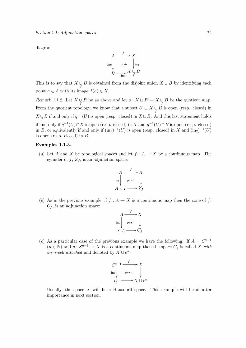
diagram
Af //
inc
push
X
in1
Bin2
// X ∪fB
This is to say that X ∪fB is obtained from the disjoint union X t B by identifying each
point a ∈ A with its image f(a) ∈ X.
Remark 1.1.2. Let X ∪fB be as above and let q : X t B → X ∪
fB be the quotient map.
From the quotient topology, we know that a subset U ⊂ X ∪fB is open (resp. closed) in
X ∪fB if and only if q−1(U) is open (resp. closed) in X tB. And this last statement holds
if and only if q−1(U)∩X is open (resp. closed) in X and q−1(U)∩B is open (resp. closed)in B, or equivalently if and only if (in1)−1(U) is open (resp. closed) in X and (in2)−1(U)is open (resp. closed) in B.
Examples 1.1.3.
(a) Let A and X be topological spaces and let f : A → X be a continuous map. Thecylinder of f , Zf , is an adjunction space:
Af //
i0
push
X
A× I // Zf
(b) As in the previous example, if f : A → X is a continuous map then the cone of f ,Cf , is an adjunction space:
Af //
inc
push
X
CA // Cf
(c) As a particular case of the previous example we have the following. If A = Sn−1
(n ∈ N) and g : Sn−1 → X is a continuous map then the space Cg is called X withan n-cell attached and denoted by X ∪ en:
Sn−1f //
inc
push
X
Dn // X ∪ en
Usually, the space X will be a Hausdorff space. This example will be of utterimportance in next section.
Section 1.1: Adjunction spaces 23
Proposition 1.1.4. Let X ∪fB be the adjunction space defined above. Then in1 : X →
X ∪fB is a closed subspace and in2|B−A : B −A→ X ∪
fB is an open subspace.
Proof. For the first statement, we have to prove that in1 is injective, initial and closed.Since in1 is continuous and injective, it suffices to prove that in1 is closed. Let F ⊆X be a closed subspace. We have that (in1)−1(in1(F )) = F which is closed in X and(in2)−1(in1(F )) = f−1(F ) which is closed in B. Hence, in1(F ) is closed in X ∪
fB.
In a similar way, for the second statement it suffices to prove that in2|B−A is an openmap. Let U ⊆ B − A be an open subspace. Since B − A is open in B, U is also open inB. Then (in1)−1(in2|B−A(U)) = ∅ and (in2)−1(in2|B−A(U)) = U . Hence, in2|B−A(U) isopen in X ∪
fB.
The following proposition stablishes conditions which assure that the adjunction spacewill be a Hausdorff space.
Proposition 1.1.5. Let X and B be Hausdorff topological spaces and let A ⊆ B be a closedsubspace. Let f : A→ X be a continuous map. Suppose that the following conditions hold:
(a) For each b ∈ B − A there exists a closed neighbourhood Cb of b in B such thatCb ∩A = ∅.
(b) There exists an open subset U ⊆ B and a retraction r : U → A.
Then the adjunction space X ∪fB is Hausdorff.
Proof. Let in1 : X → X ∪fB and in2 : B → X ∪
fB be as in the definition of adjuntion
spaces and let x1, x2 ∈ X ∪fB. We must find disjoint open subsets V1, V2 ⊆ X ∪
fB such
that x1 ∈ V1 and x2 ∈ V2. We divide the proof in three cases.(1) x1, x2 ∈ B − A. Since B − A is Hausdorff there exist open and disjoint subsets
V1, V2 ⊆ B − A such that x1 ∈ V1 and x2 ∈ V2. But B − A is open in X ∪fB by the
previous proposition, hence V1 and V2 are also open in X ∪fB.
(2) x1 ∈ X and x2 ∈ B − A. We take V1 = X ∪fB − Cx2 and V2 = (Cx2)
. Note
that (in1)−1(V1) = X, (in2)−1(V1) = B − Cx2 , (in1)−1(V2) = ∅ and (in2)−1(V2) = (Cx2).
Hence V1 and V2 are open in X ∪fB.
(3) x1, x2 ∈ X. Since X is Hausdorff there exist open and disjoint subsets W1,W2 ⊆ Xsuch that x1 ∈ W1 and x2 ∈ W2. But W1 and W2 might not be open in X ∪
fB. Using
the retraction r we will enlarge the subsets W1 and W2 so that they are open in X ∪fB
and remain disjoint. We take V1 = W1 ∪ r−1f−1(W1) and V2 = W2 ∪ r−1f−1(W2).Note that V1 ∩ V2 = ∅ and that V1 and V2 are open in X ∪
fB since (in1)−1(Vi) = Wi,
(in2)−1(Vi) = r−1f−1(Wi) for i = 1, 2.
Section 1.1: Adjunction spaces 24
Important remark 1.1.6. If we take A = Sn−1 and B = Dn then conditions (a) and(b) of the previous proposition hold. The same happens if we take A =
⊔i∈ISn−1 and
B =⊔i∈IDn.
We want now to find conditions for two adjunction spaces to be homotopy equivalent.To this end, we will need to work with cofibrations.
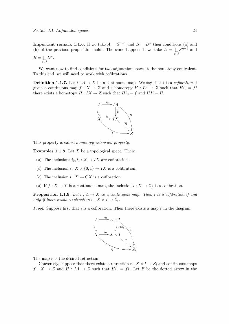
Definition 1.1.7. Let i : A → X be a continuous map. We say that i is a cofibration ifgiven a continuous map f : X → Z and a homotopy H : IA → Z such that Hi0 = fithere exists a homotopy H : IX → Z such that Hi0 = f and HIi = H.
Ai0 //
i
IA
Ii H
Xi0 //
f 00
IXH
!!Z
This property is called homotopy extension property.
Examples 1.1.8. Let X be a topological space. Then:
(a) The inclusions i0, i1 : X → IX are cofibrations.
(b) The inclusion i : X × 0, 1 → IX is a cofibration.
(c) The inclusion i : X → CX is a cofibration.
(d) If f : X → Y is a continuous map, the inclusion i : X → Zf is a cofibration.
Proposition 1.1.9. Let i : A → X be a continuous map. Then i is a cofibration if andonly if there exists a retraction r : X × I → Zi.
Proof. Suppose first that i is a cofibration. Then there exists a map r in the diagram
Ai0 //
i
A× I
i×IdI
i1
Xi0 //
i2 00
X × Ir
##Zi
The map r is the desired retraction.Conversely, suppose that there exists a retraction r : X × I → Zi and continuous maps
f : X → Z and H : IA → Z such that Hi0 = fi. Let F be the dotted arrow in the
Section 1.1: Adjunction spaces 25
diagram
Ai0 //
i
push
A× I
i×IdI
H
Xi0 //
f 00
ZiF
""Z
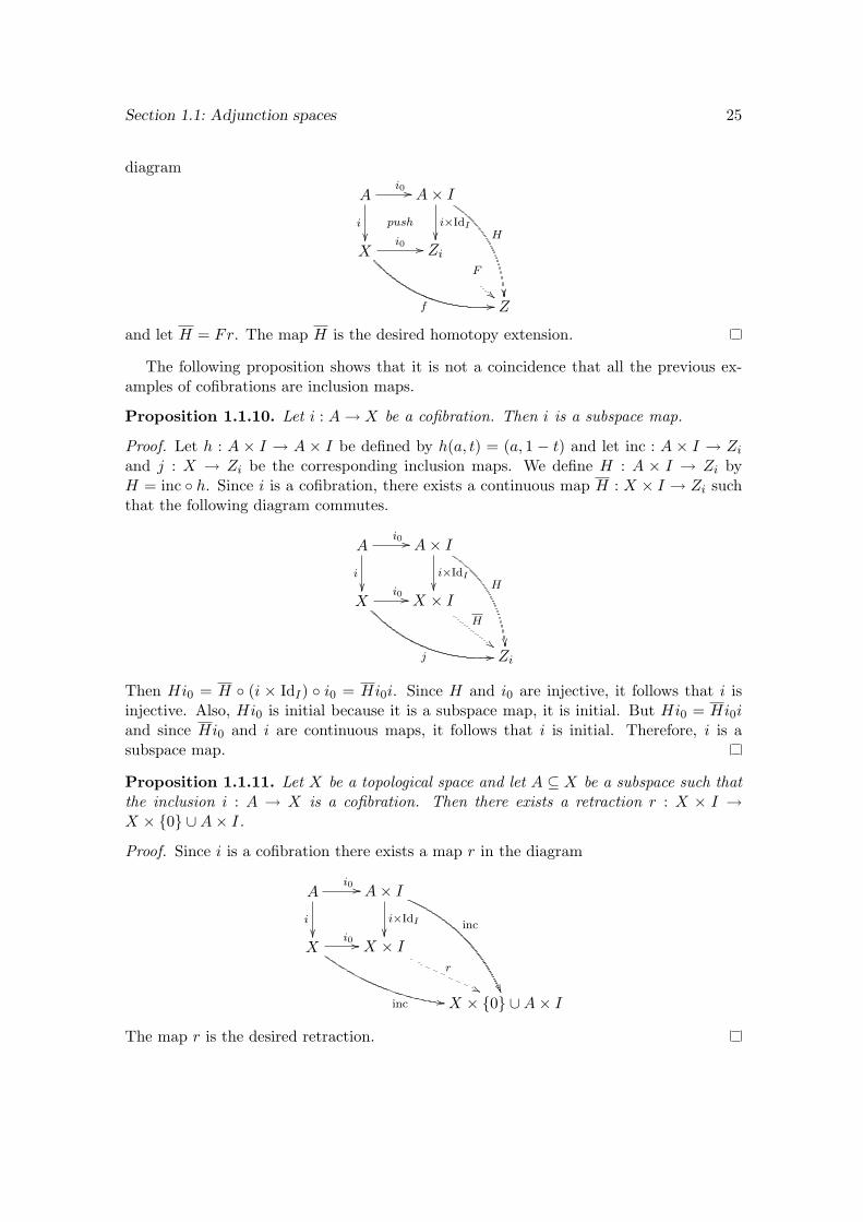
and let H = Fr. The map H is the desired homotopy extension.
The following proposition shows that it is not a coincidence that all the previous ex-amples of cofibrations are inclusion maps.
Proposition 1.1.10. Let i : A→ X be a cofibration. Then i is a subspace map.
Proof. Let h : A × I → A × I be defined by h(a, t) = (a, 1 − t) and let inc : A × I → Ziand j : X → Zi be the corresponding inclusion maps. We define H : A × I → Zi byH = inc h. Since i is a cofibration, there exists a continuous map H : X × I → Zi suchthat the following diagram commutes.
Ai0 //
i
A× I
i×IdI
H
Xi0 //
j 00
X × IH
##Zi
Then Hi0 = H (i × IdI) i0 = Hi0i. Since H and i0 are injective, it follows that i isinjective. Also, Hi0 is initial because it is a subspace map, it is initial. But Hi0 = Hi0iand since Hi0 and i are continuous maps, it follows that i is initial. Therefore, i is asubspace map.
Proposition 1.1.11. Let X be a topological space and let A ⊆ X be a subspace such thatthe inclusion i : A → X is a cofibration. Then there exists a retraction r : X × I →X × 0 ∪A× I.
Proof. Since i is a cofibration there exists a map r in the diagram
Ai0 //
i
A× I
i×IdI
inc
Xi0 //
inc --
X × Ir
''X × 0 ∪A× I
The map r is the desired retraction.
Section 1.1: Adjunction spaces 26
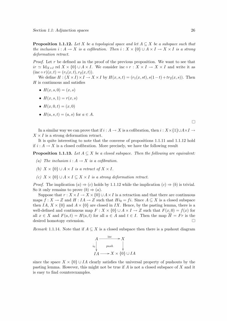
Proposition 1.1.12. Let X be a topological space and let A ⊆ X be a subspace such thatthe inclusion i : A → X is a cofibration. Then i : X × 0 ∪ A × I → X × I is a strongdeformation retract.
Proof. Let r be defined as in the proof of the previous proposition. We want to see thatir ' IdX×I rel X × 0 ∪A× I. We consider inc r : X × I → X × I and write it as(inc r)(x, t) = (r1(x, t), r2(x, t)).
We define H : (X× I)× I → X× I by H(x, s, t) = (r1(x, st), s(1− t)+ tr2(x, s)). ThenH is continuous and satisfies
• H(x, s, 0) = (x, s)
• H(x, s, 1) = r(x, s)
• H(x, 0, t) = (x, 0)
• H(a, s, t) = (a, s) for a ∈ A.
In a similar way we can prove that if i : A→ X is a cofibration, then i : X×1∪A×I →X × I is a strong deformation retract.
It is quite interesting to note that the converse of propositions 1.1.11 and 1.1.12 holdif i : A→ X is a closed cofibration. More precisely, we have the following result
Proposition 1.1.13. Let A ⊆ X be a closed subspace. Then the following are equivalent:
(a) The inclusion i : A→ X is a cofibration.
(b) X × 0 ∪A× I is a retract of X × I.
(c) X × 0 ∪A× I ⊆ X × I is a strong deformation retract.
Proof. The implication (a) ⇒ (c) holds by 1.1.12 while the implication (c) ⇒ (b) is trivial.So it only remains to prove (b) ⇒ (a).
Suppose that r : X× I → X×0∪A× I is a retraction and that there are continuousmaps f : X → Z and H : IA→ Z such that Hi0 = fi. Since A ⊆ X is a closed subspacethen IA, X × 0 and A× 0 are closed in IX. Hence, by the pasting lemma, there is awell-defined and continuous map F : X × 0 ∪ A × I → Z such that F (x, 0) = f(x) forall x ∈ X and F (a, t) = H(a, t) for all a ∈ A and t ∈ I. Then the map H = Fr is thedesired homotopy extension.
Remark 1.1.14. Note that if A ⊆ X is a closed subspace then there is a pushout diagram
Ainc //
i0
push
X
IA // X × 0 ∪ IA
since the space X × 0 ∪ IA clearly satisfies the universal property of pushouts by thepasting lemma. However, this might not be true if A is not a closed subspace of X and itis easy to find counterexamples.
Section 1.1: Adjunction spaces 27
The following proposition follows from the exponential law
Proposition 1.1.15. If i : A→ X is a cofibration then Ii : IA→ IX is also a cofibration.
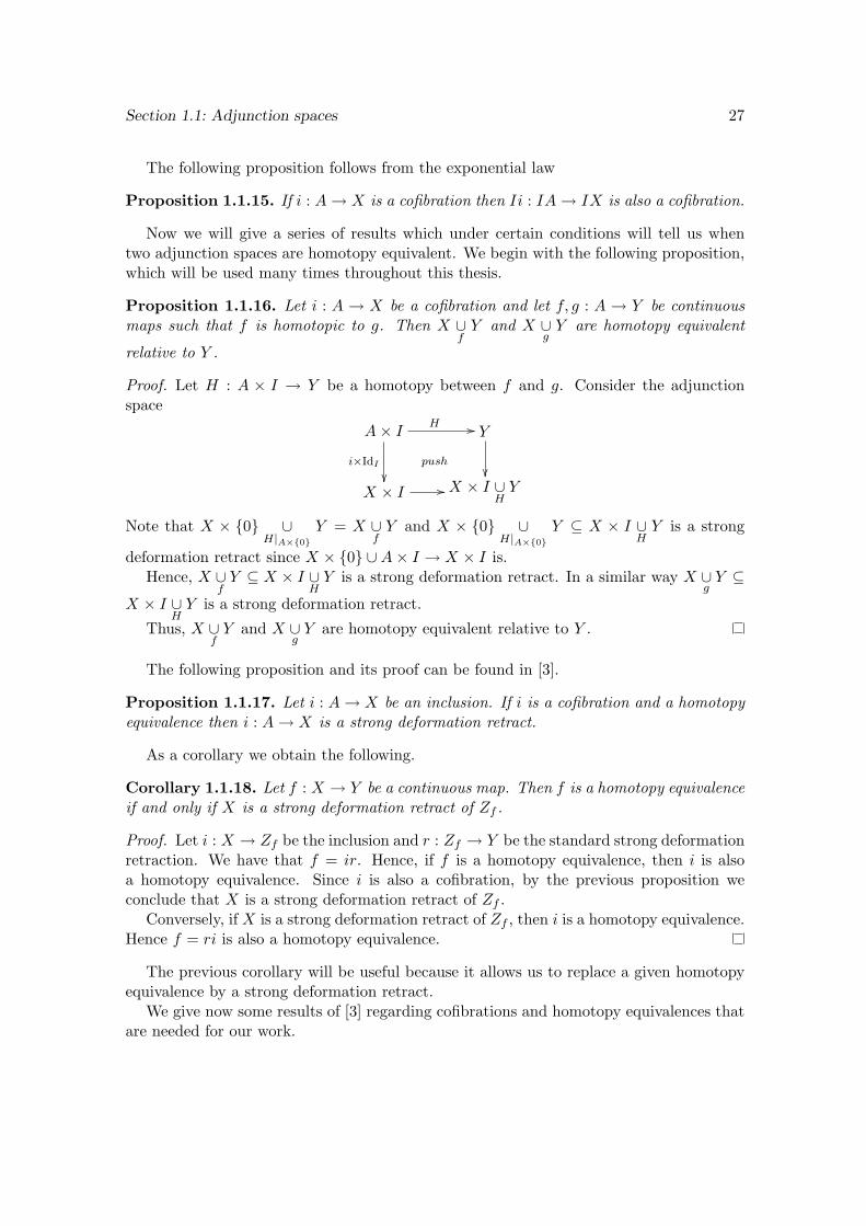
Now we will give a series of results which under certain conditions will tell us whentwo adjunction spaces are homotopy equivalent. We begin with the following proposition,which will be used many times throughout this thesis.
Proposition 1.1.16. Let i : A → X be a cofibration and let f, g : A → Y be continuousmaps such that f is homotopic to g. Then X ∪
fY and X ∪
gY are homotopy equivalent
relative to Y .
Proof. Let H : A × I → Y be a homotopy between f and g. Consider the adjunctionspace
A× IH //
i×IdI
push
Y
X × I // X × I ∪HY
Note that X × 0 ∪H|A×0
Y = X ∪fY and X × 0 ∪
H|A×0Y ⊆ X × I ∪
HY is a strong
deformation retract since X × 0 ∪A× I → X × I is.Hence, X ∪
fY ⊆ X × I ∪
HY is a strong deformation retract. In a similar way X ∪
gY ⊆
X × I ∪HY is a strong deformation retract.
Thus, X ∪fY and X ∪
gY are homotopy equivalent relative to Y .
The following proposition and its proof can be found in [3].
Proposition 1.1.17. Let i : A→ X be an inclusion. If i is a cofibration and a homotopyequivalence then i : A→ X is a strong deformation retract.
As a corollary we obtain the following.
Corollary 1.1.18. Let f : X → Y be a continuous map. Then f is a homotopy equivalenceif and only if X is a strong deformation retract of Zf .
Proof. Let i : X → Zf be the inclusion and r : Zf → Y be the standard strong deformationretraction. We have that f = ir. Hence, if f is a homotopy equivalence, then i is alsoa homotopy equivalence. Since i is also a cofibration, by the previous proposition weconclude that X is a strong deformation retract of Zf .
Conversely, if X is a strong deformation retract of Zf , then i is a homotopy equivalence.Hence f = ri is also a homotopy equivalence.
The previous corollary will be useful because it allows us to replace a given homotopyequivalence by a strong deformation retract.
We give now some results of [3] regarding cofibrations and homotopy equivalences thatare needed for our work.
Section 1.1: Adjunction spaces 28
Proposition 1.1.19. Let X and B be topological spaces and let A ⊆ B be a closed subspacesuch that the inclusion i : A → B is a cofibration. Let f, g : A → X be continuous mapssuch that f ' g. Then X ∪
fB ' X ∪
gB rel X.
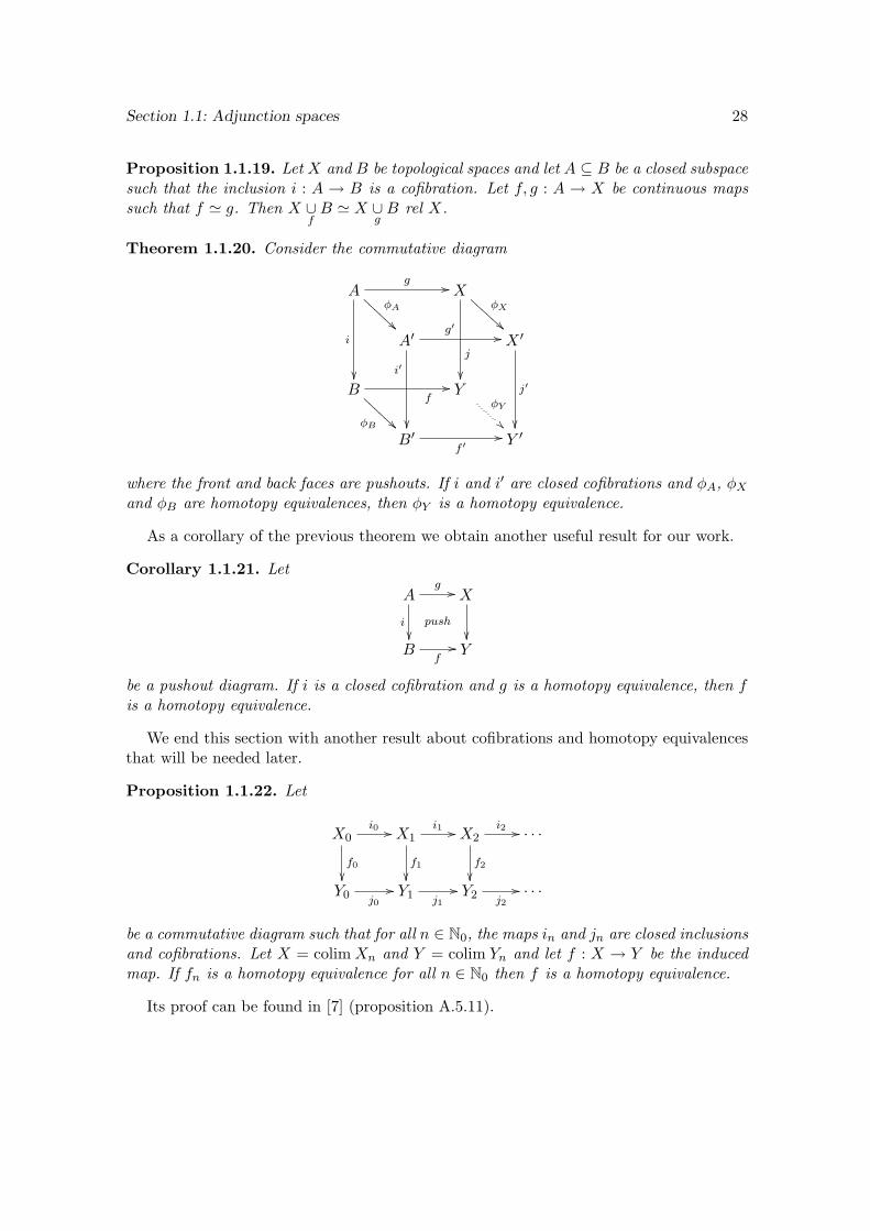
Theorem 1.1.20. Consider the commutative diagram
Ag //
i
φA
AAA
AAA X
j
φX
BBB
BBB
A′g′ //
i′
X ′
j′
Bf//
φB AAA
AAA Y
φY
B′
f ′// Y ′
where the front and back faces are pushouts. If i and i′ are closed cofibrations and φA, φXand φB are homotopy equivalences, then φY is a homotopy equivalence.
As a corollary of the previous theorem we obtain another useful result for our work.
Corollary 1.1.21. Let
Ag //
ipush
X
B
f// Y
be a pushout diagram. If i is a closed cofibration and g is a homotopy equivalence, then fis a homotopy equivalence.
We end this section with another result about cofibrations and homotopy equivalencesthat will be needed later.
Proposition 1.1.22. Let
X0i0 //
f0
X1i1 //
f1
X2i2 //
f2
. . .
Y0 j0// Y1 j1
// Y2 j2// . . .
be a commutative diagram such that for all n ∈ N0, the maps in and jn are closed inclusionsand cofibrations. Let X = colimXn and Y = colim Yn and let f : X → Y be the inducedmap. If fn is a homotopy equivalence for all n ∈ N0 then f is a homotopy equivalence.
Its proof can be found in [7] (proposition A.5.11).
Section 1.2: Definition of CW-complexes 29
1.2 Definition of CW-complexes
In this section we recall the definition of CW-complexes and some standard examplesand basic properties. We analize both the constructive and descriptive approachs and weprove that they are equivalent. Finally, we give the definition of subcomplexes and relativeCW-complexes and we study product cellular structures.
1.2.1 Constructive definition
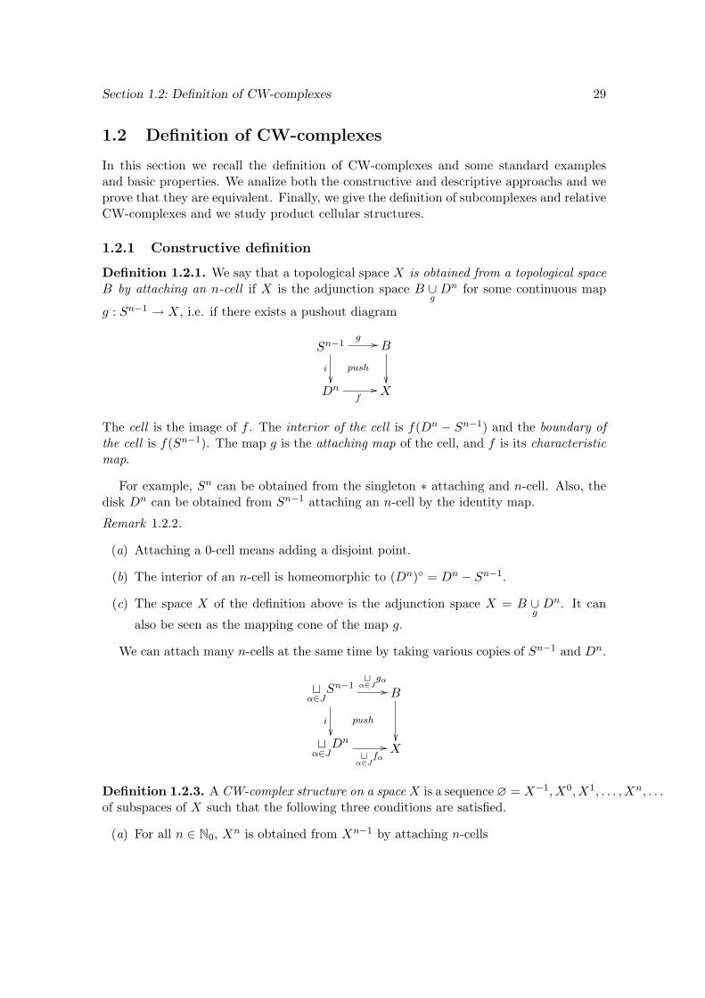
Definition 1.2.1. We say that a topological space X is obtained from a topological spaceB by attaching an n-cell if X is the adjunction space B ∪
gDn for some continuous map
g : Sn−1 → X, i.e. if there exists a pushout diagram
Sn−1g //
i
push
B
Dn
f// X
The cell is the image of f . The interior of the cell is f(Dn − Sn−1) and the boundary ofthe cell is f(Sn−1). The map g is the attaching map of the cell, and f is its characteristicmap.
For example, Sn can be obtained from the singleton ∗ attaching and n-cell. Also, thedisk Dn can be obtained from Sn−1 attaching an n-cell by the identity map.
Remark 1.2.2.
(a) Attaching a 0-cell means adding a disjoint point.
(b) The interior of an n-cell is homeomorphic to (Dn) = Dn − Sn−1.
(c) The space X of the definition above is the adjunction space X = B ∪gDn. It can
also be seen as the mapping cone of the map g.
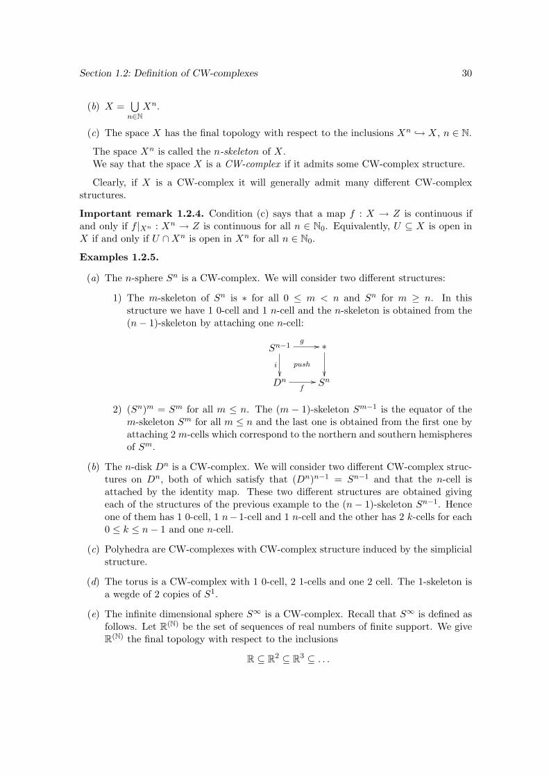
We can attach many n-cells at the same time by taking various copies of Sn−1 and Dn.
tα∈J
Sn−1t
α∈Jgα
//
i
push
B
tα∈J
Dn
tα∈J
fα
// X
Definition 1.2.3. A CW-complex structure on a space X is a sequence ∅ = X−1, X0, X1, . . . , Xn, . . .of subspaces of X such that the following three conditions are satisfied.
(a) For all n ∈ N0, Xn is obtained from Xn−1 by attaching n-cells
Section 1.2: Definition of CW-complexes 30
(b) X =⋃n∈N
Xn.
(c) The space X has the final topology with respect to the inclusions Xn → X, n ∈ N.
The space Xn is called the n-skeleton of X.We say that the space X is a CW-complex if it admits some CW-complex structure.
Clearly, if X is a CW-complex it will generally admit many different CW-complexstructures.
Important remark 1.2.4. Condition (c) says that a map f : X → Z is continuous ifand only if f |Xn : Xn → Z is continuous for all n ∈ N0. Equivalently, U ⊆ X is open inX if and only if U ∩Xn is open in Xn for all n ∈ N0.
Examples 1.2.5.
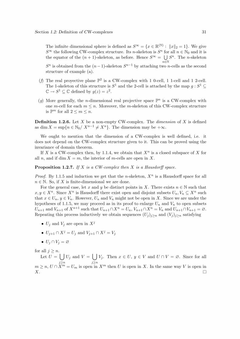
(a) The n-sphere Sn is a CW-complex. We will consider two different structures:
1) The m-skeleton of Sn is ∗ for all 0 ≤ m < n and Sn for m ≥ n. In thisstructure we have 1 0-cell and 1 n-cell and the n-skeleton is obtained from the(n− 1)-skeleton by attaching one n-cell:
Sn−1g //
i
push
∗
Dn
f// Sn
2) (Sn)m = Sm for all m ≤ n. The (m − 1)-skeleton Sm−1 is the equator of them-skeleton Sm for all m ≤ n and the last one is obtained from the first one byattaching 2 m-cells which correspond to the northern and southern hemispheresof Sm.
(b) The n-disk Dn is a CW-complex. We will consider two different CW-complex struc-tures on Dn, both of which satisfy that (Dn)n−1 = Sn−1 and that the n-cell isattached by the identity map. These two different structures are obtained givingeach of the structures of the previous example to the (n− 1)-skeleton Sn−1. Henceone of them has 1 0-cell, 1 n− 1-cell and 1 n-cell and the other has 2 k-cells for each0 ≤ k ≤ n− 1 and one n-cell.
(c) Polyhedra are CW-complexes with CW-complex structure induced by the simplicialstructure.
(d) The torus is a CW-complex with 1 0-cell, 2 1-cells and one 2 cell. The 1-skeleton isa wegde of 2 copies of S1.
(e) The infinite dimensional sphere S∞ is a CW-complex. Recall that S∞ is defined asfollows. Let R(N) be the set of sequences of real numbers of finite support. We giveR(N) the final topology with respect to the inclusions
R ⊆ R2 ⊆ R3 ⊆ . . .
Section 1.2: Definition of CW-complexes 31
The infinite dimensional sphere is defined as S∞ = x ∈ R(N) : ‖x‖2 = 1. We giveS∞ the following CW-complex structure. Its n-skeleton is Sn for all n ∈ N0 and it isthe equator of the (n + 1)-skeleton, as before. Hence S∞ =
⋃n∈N
Sn. The n-skeleton
Sn is obtained from the (n−1)-skeleton Sn−1 by attaching two n-cells as the secondstructure of example (a).
(f) The real proyective plane P2 is a CW-complex with 1 0-cell, 1 1-cell and 1 2-cell.The 1-skeleton of this structure is S1 and the 2-cell is attached by the map g : S1 ⊆C → S1 ⊆ C defined by g(z) = z2.
(g) More generally, the n-dimensional real projective space Pn is a CW-complex withone m-cell for each m ≤ n. Moreover, the m-skeleton of this CW-complex structureis Pm for all 2 ≤ m ≤ n.
Definition 1.2.6. Let X be a non-empty CW-complex. The dimension of X is definedas dimX = supn ∈ N0/ X
n−1 6= Xn. The dimension may be +∞.
We ought to mention that the dimension of a CW-complex is well defined, i.e. itdoes not depend on the CW-complex structure given to it. This can be proved using theinvariance of domain theorem.
If X is a CW-complex then, by 1.1.4, we obtain that Xn is a closed subspace of X forall n, and if dimX = m, the interior of m-cells are open in X.
Proposition 1.2.7. If X is a CW-complex then X is a Hausdorff space.
Proof. By 1.1.5 and induction we get that the n-skeleton, Xn is a Hausdorff space for alln ∈ N. So, if X is finite-dimensional we are done.
For the general case, let x and y be distinct points in X. There exists n ∈ N such thatx, y ∈ Xn. Since Xn is Hausdorff there exist open and disjoint subsets Un, Vn ⊆ Xn suchthat x ∈ Un, y ∈ Vn. However, Un and Vn might not be open in X. Since we are under thehypotheses of 1.1.5, we may proceed as in its proof to enlarge Un and Vn to open subsetsUn+1 and Vn+1 of Xn+1 such that Un+1∩Xn = Un, Vn+1∩Xn = Vn and Un+1∩Vn+1 = ∅.Repeating this process inductively we obtain sequences (Uj)j≥n and (Vj)j≥n satisfying
• Uj and Vj are open in Xj
• Uj+1 ∩Xj = Uj and Vj+1 ∩Xj = Vj
• Uj ∩ Vj = ∅
for all j ≥ n.Let U =
⋃j≥n
Uj and V =⋃j≥n
Vj . Then x ∈ U , y ∈ V and U ∩ V = ∅. Since for all
m ≥ n, U ∩Xm = Um is open in Xm then U is open in X. In the same way V is open inX.
Section 1.2: Definition of CW-complexes 32
1.2.2 Descriptive definition
Definition 1.2.8. Let X be a Hausdorff space. A cell complex on a space X is a collectionK = enα : n ∈ N0, α ∈ Jn of subsets of X, called cells, which satisfy the properties below.The cell enα is called a cell of dimension n or n-cell and the set Jn, n ∈ N is an index setfor the n-cells.
For n ≥ 0, we define the n-skeleton of K as Kn = erα : r ≤ n, α ∈ Jr. We also defineK−1 = ∅. Let |Kn| =
⋃r≤nα∈Jr
erα ⊆ X.
For each cell enα we define the boundary of enα as•enα = enα ∩ |Kn−1| and the interior of
enα asenα = enα −
•enα.
The collection K must satisfy
(a) X =⋃n,α
enα
(b)enα ∩
emβ = ∅ if enα 6= emβ
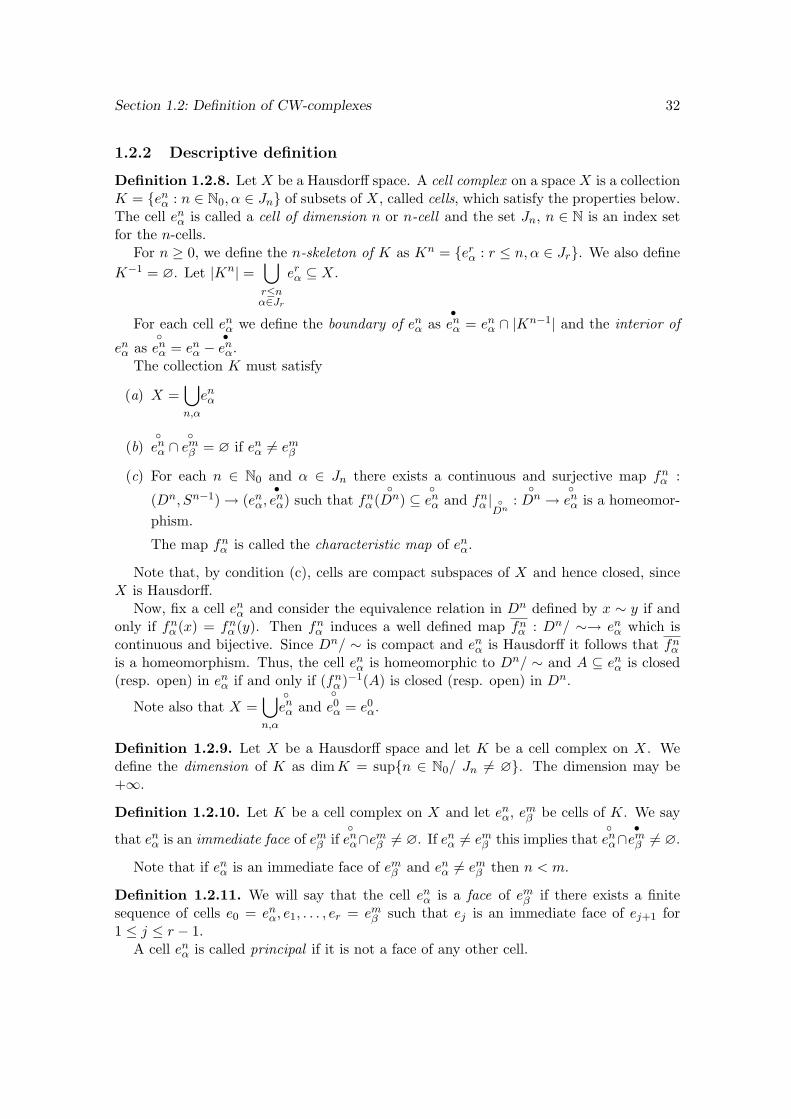
(c) For each n ∈ N0 and α ∈ Jn there exists a continuous and surjective map fnα :
(Dn, Sn−1) → (enα,•enα) such that fnα (
Dn) ⊆
enα and fnα |
Dn:Dn →
enα is a homeomor-
phism.
The map fnα is called the characteristic map of enα.
Note that, by condition (c), cells are compact subspaces of X and hence closed, sinceX is Hausdorff.
Now, fix a cell enα and consider the equivalence relation in Dn defined by x ∼ y if andonly if fnα (x) = fnα (y). Then fnα induces a well defined map fnα : Dn/ ∼→ enα which iscontinuous and bijective. Since Dn/ ∼ is compact and enα is Hausdorff it follows that fnαis a homeomorphism. Thus, the cell enα is homeomorphic to Dn/ ∼ and A ⊆ enα is closed(resp. open) in enα if and only if (fnα )−1(A) is closed (resp. open) in Dn.
Note also that X =⋃n,α
enα and
e0α = e0α.
Definition 1.2.9. Let X be a Hausdorff space and let K be a cell complex on X. Wedefine the dimension of K as dimK = supn ∈ N0/ Jn 6= ∅. The dimension may be+∞.
Definition 1.2.10. Let K be a cell complex on X and let enα, emβ be cells of K. We say
that enα is an immediate face of emβ ifenα∩emβ 6= ∅. If enα 6= emβ this implies that
enα∩
•emβ 6= ∅.
Note that if enα is an immediate face of emβ and enα 6= emβ then n < m.
Definition 1.2.11. We will say that the cell enα is a face of emβ if there exists a finitesequence of cells e0 = enα, e1, . . . , er = emβ such that ej is an immediate face of ej+1 for1 ≤ j ≤ r − 1.
A cell enα is called principal if it is not a face of any other cell.
Section 1.2: Definition of CW-complexes 33
Note that the faces of a cell enα are exactly those cells which we must attach first inorder to be able to attach the cell enα. This intuitive statement will become clearer afterintroducing the notion of subcomplexes in subsection 1.1.4.
Remark 1.2.12. A cell complex K on X does not give much information on the topologyof X. For example, we may take K = X, that is every point of X is a 0-cell. This is a cellcomplex which does not give any data on the topology of X.
This is certainly not among the sort of things one would like to accept. So we willimpose two extra conditions on a cell complex to call it a CW-complex.
Definition 1.2.13. Let X be a Hausdorff space. A CW-complex structure on X is a cellcomplex K such that the following conditions are satisfied:
(C) Each cell of K has only a finite number of faces.
(W) The space X has the weak topology induced by the cells of K, that is, A ⊆ X isclosed if and only if A ∩ enα is closed in enα for all n ∈ N, α ∈ Jn.
A space X is called a CW-complex if it admits some CW-complex structure.The following propositions follow easily from the definition of cell complex and condition
(W).
Proposition 1.2.14. If X is a CW-complex and enα is a principal cell, thenenα is open in
X.
Condition (W) can also be stated in a couple of other ways, which allow us to understandtopology of CW-complexes better.
Proposition 1.2.15. Let X be a CW-complex with CW-structure K. The following areequivalent:
(a) A ⊆ X is closed (resp. open).
(b) A ∩ enα is closed (resp. open) in enα for all n, α.
(c) (fnα )−1(A) ⊆ Dn is closed (resp. open) for all n, α.
(d) A ∩ |Kn| is closed (resp. open) in |Kn| for all n.
These equivalent statements can be reformulated in terms of continuous maps as nextproposition shows.
Proposition 1.2.16. Let X be a CW-complex with CW-structure K, let Y be a topologicalspace and let f : X → Y be a map. Then the following are equivalent:
(a) f : X → Y is continuous.
(b) f |enα
: enα → Y is continuous for all n, α.
(c) f fnα : Dn → Y is continuous for all n, α.
Section 1.2: Definition of CW-complexes 34
(d) f ||Kn| is continuous for all n.
This proposition will be useful when defining maps with domain a CW-complex. Usu-ally, we will define maps skeleton by skeleton, continuous at each stage, and by the equiv-alences above we will conclude that they are continuous.
The same argument will be used when defining homotopies from CW-complexes. Thefollowing is the analogous of the previous proposition and follows from it applying theexponential law.
Proposition 1.2.17. Let X be a CW-complex with CW-structure K, let Y be a topologicalspace and let H : X × I → Y be a map. Then the following are equivalent:
(a) H : X × I → Y is continuous.
(b) H|enα×I : enα × I → Y is continuous for all n, α.
(c) H (fnα × IdI) : Dn × I → Y is continuous for all n, α.
(d) H||Kn|×I is continuous for all n.
The next proposition shows a key point in the theory of CW-complexes, as will beevident later on.
Proposition 1.2.18. Let X be a CW-complex and let K ⊆ X be a compact subset. ThenK intersects only a finite number of interiors of cells.
In particular, X is compact if and only if it is finite (i.e. has a finite number of cells).
Proof. For each n and α such that K ∩enα 6= ∅ we choose xnα ∈ C ∩
enα. Let T = xnα : n ∈
N0, α ∈ Jn. Then T ⊆ K. We shall prove that T is finite.We will show that T ⊆ K is closed (hence compact) and discrete. It suffices to prove
that every T ′ ⊆ T is closed in X.By (W), T ′ ⊆ X is closed if and only if T ′ ∩ enα is closed in enα for all n, α. But by
(C), each cell has a finite number of faces, hence T ′ ∩ enα is finite. Since X is Hausdorff itfollows that T ′ ∩ enα is closed in X. Thus, T ′ is closed in X for all T ′ ⊆ T .
The following remark will be very important for our descriptive definition of CW(A)-complexes (cf. 3.2.2) since it gives us the right way to generalize the descriptive definitionof CW-complexes.
Important remark 1.2.19. Conditions (C) and (W) are equivalent to (C’) and (W)where
(C’) Every compact subspace intersects only a finite number of interiors of cells.
Indeed, (C) and (W) imply (C’) and (W) by the previous proposition. Conversely, (C’)implies (C) because cells are compact subspaces.
Section 1.2: Definition of CW-complexes 35
1.2.3 Equivalence of both definitions
We will show now that both definitions are equivalent. The first implication is stated inthe following proposition, which is easy to prove.
Proposition 1.2.20. Let X be a Hausdorff topological space and let K be a CW-complexstructure on X. Then X is a constructive CW-complex (i.e. according to definition 1.2.3)where the skeletons Xn coincide with |Kn| and where the characteristic maps of the cellsare the same in both structures.
For the converse we need the following lemma.
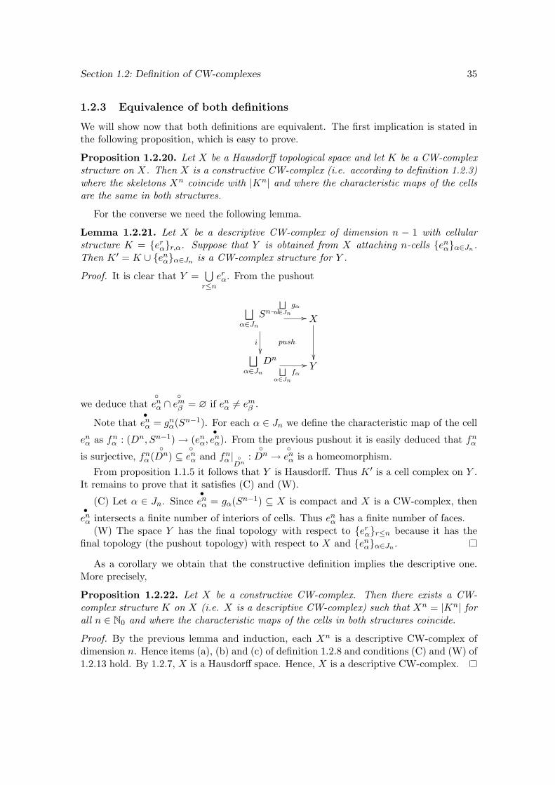
Lemma 1.2.21. Let X be a descriptive CW-complex of dimension n − 1 with cellularstructure K = erαr,α. Suppose that Y is obtained from X attaching n-cells enαα∈Jn.Then K ′ = K ∪ enαα∈Jn is a CW-complex structure for Y .
Proof. It is clear that Y =⋃r≤n
erα. From the pushout
⊔α∈Jn
Sn−1
Fα∈Jn
gα
//
i
push
X
⊔α∈Jn
Dn Fα∈Jn
fα
// Y
we deduce thatenα ∩
emβ = ∅ if enα 6= emβ .
Note that•enα = gnα(Sn−1). For each α ∈ Jn we define the characteristic map of the cell
enα as fnα : (Dn, Sn−1) → (enα,•enα). From the previous pushout it is easily deduced that fnα
is surjective, fnα (Dn) ⊆
enα and fnα |
Dn:Dn →
enα is a homeomorphism.
From proposition 1.1.5 it follows that Y is Hausdorff. Thus K ′ is a cell complex on Y .It remains to prove that it satisfies (C) and (W).
(C) Let α ∈ Jn. Since•enα = gα(Sn−1) ⊆ X is compact and X is a CW-complex, then
•enα intersects a finite number of interiors of cells. Thus enα has a finite number of faces.
(W) The space Y has the final topology with respect to erαr≤n because it has thefinal topology (the pushout topology) with respect to X and enαα∈Jn .
As a corollary we obtain that the constructive definition implies the descriptive one.More precisely,
Proposition 1.2.22. Let X be a constructive CW-complex. Then there exists a CW-complex structure K on X (i.e. X is a descriptive CW-complex) such that Xn = |Kn| forall n ∈ N0 and where the characteristic maps of the cells in both structures coincide.
Proof. By the previous lemma and induction, each Xn is a descriptive CW-complex ofdimension n. Hence items (a), (b) and (c) of definition 1.2.8 and conditions (C) and (W) of1.2.13 hold. By 1.2.7, X is a Hausdorff space. Hence, X is a descriptive CW-complex.
Section 1.2: Definition of CW-complexes 36
1.2.4 Subcomplexes and relative CW-complexes
We give first a quick glance at subcomplexes. As mentioned before, given a cell enα, itsfaces can be interpreted as the cells that need to be pasted first so that the cell enα can beattached. For if any of the immediate faces of enα is not attached first then the adjunctionmap of enα will not be well defined. A similar argument applies for the immediate faces ofenα, and repeating this process we get the statement.
Definition 1.2.23. Let K be a cell complex on X. Let L ⊆ K. We say that L is asubcomplex of K if for each cell enα ∈ L all its faces also belong to L.
The following proposition enlights and justifies the definition above.
Proposition 1.2.24. Let X be a topological space, K a cell complex on X and L ⊆ K asubcomplex. Let |L| =
⋃enα∈L
enα ⊆ X with the subspace topology. Then
(a) L is a cell complex on |L| with structure inherited from K (i.e. the characteristicmaps are the same).
(b) If K is a CW-complex structure on X then L is a CW-complex structure on |L|.
(c) |L| is closed in X.
Definition 1.2.25. A CW-pair is a topological pair (X,A) where X is a CW-complexand A ⊆ X is a subcomplex.
In the constructive definition of CW-complexes we begin with the empty set and startattaching cells of different dimensions. If instead we begin with a Hausdorff topologicalspace A, the space obtained is called relative CW-complex.
Definition 1.2.26. A relative CW-complex is a pair (X,A), where A and X are topolog-ical spaces such that A ⊆ X, A is Hausdorff and there exists a sequence of subspaces ofX
A = X−1A ⊆ X0
A ⊆ X1A ⊆ . . . ⊆ Xn
A ⊆ . . .
satisfying that, for all n ∈ N0, XnA is obtained from Xn−1
A by attaching n-cells, X =⋃n∈N
XnA
and X has the final topology with respect to XnAn≥−1.
As in the absolute case, the subspace XnA is called the n-skeleton of (X,A).
Remark 1.2.27.
(a) Let (X,A) be a relative CW-complex. Then X is Hausdorff and A ⊆ X is a closedsubspace.
(b) If (X,A) is a CW-pair, then it is a relative CW-complex.
Definition 1.2.28. Let X and Y be CW-complexes. A continuous map f : X → Y iscalled cellular if f(Xn) ⊆ Y n for all n ≥ 0.
Proposition 1.2.29. Let X and Y be CW-complexes and let f : X → Y be a cellularmap. Then the cylinder of f , Zf , is a CW-complex and X ⊆ Zf is subcomplex.
Section 1.2: Definition of CW-complexes 37
1.2.5 Product of cellular spaces
We want to give a CW-complex structure to the cartesian product of CW-complexes. Notethat Dn ×Dm is homeomorphic to Dn+m. Hence, if X is a CW-complex with structureK and Y is a CW-complex with structure K ′, it is reasonable that cells of the cartesianproduct X × Y would be products of one cell of K with one cell of K ′. However, theproduct topology in X × Y is not always the right one, as we shall see.
If K = enαn,α is a cellular structure in a Hausdorff space X and K ′ = emβ m,β is acellular structure in another Hausdorff space Y , we define the product cellular structurein X × Y by K × K ′ = enα × emβ n,m,α,β . It is easy to prove that K × K ′ is a cellularstructure in X × Y .
It is clear that if the cellular structures K and K ′ satisfy condition (C) then K ×K ′
also satisfies (C). However, this is not always true for condition (W). Hence we define thefollowing.
Definition 1.2.30. Let X and Y be CW-complexes with cellular structures K and K ′
respectively. We define the CW-complex X×wY as the space X×Y with cellular structure
K ×K ′ and with the final topology with respect to the cells of K ×K ′, i.e. F ⊆ X × Yis closed if and only if F ∩ (enα × emβ ) is closed in enα × emβ for all cells enα × emβ ∈ K ×K ′.
Note that the weak topology in X × Y (that is, the final topology with respect to thecells) has fewer open sets than the product topology. Nevertheless, the subspace topologyin enα × emβ is the same for both topologies.
The next proposition is not difficult to prove and stablishes a relation between bothtopologies.
Proposition 1.2.31. Let X and Y be CW-complexes. If X or Y is locally compact thenX ×
wY = X × Y .
In particular, if we take Y = I with cellular structure e00 = 0, e01 = 1, e1 = Iand X is a CW-complex with cellular structure K, then X × I is also a CW-complexand its cellular structure is enα × e00, e
nα × e01, e
nα × e1 : enα ∈ K. Note that enα × e00 and
enα × e01 are n-cells and enα × e1 is a (n + 1)-cell. Hence, if X is finite dimensional thendim(X × I) = dim(X) + 1.
The following proposition sums up several properties of CW-complexes.
Proposition 1.2.32.
(a) Let (X,A) be a relative CW-complex. Then X/A is a CW-complex with cellularstructure inherited from (X,A).
(b) If X is obtained from A by attaching n-cells then X/A =∨
α∈Jn
Sn (where Jn is the
set that indexes the n-cells).
Moreover, there is a homeomorphism between X/A and∨
α∈Jn
Sn such that the follow-
ing diagram commutes for all α ∈ Jn.
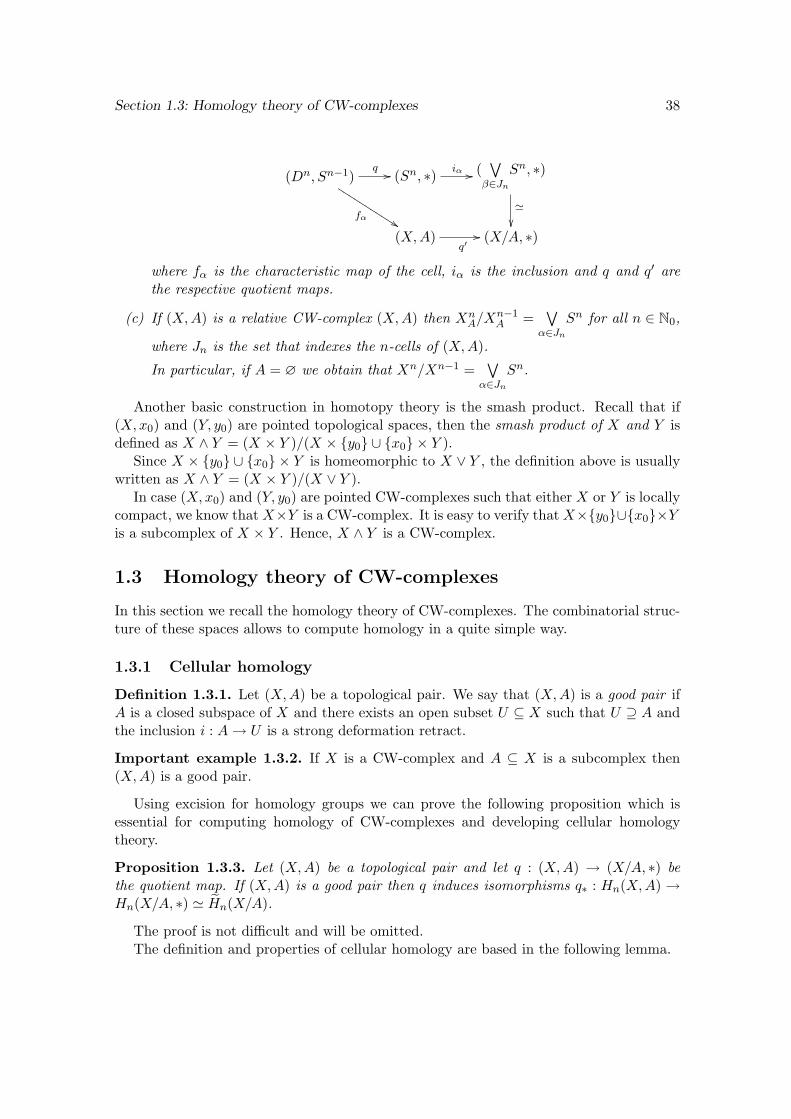
Section 1.3: Homology theory of CW-complexes 38
(Dn, Sn−1)q //
fα %%KKKKKKKKKKK(Sn, ∗) iα // (
∨β∈Jn
Sn, ∗)
'
(X,A)q′// (X/A, ∗)
where fα is the characteristic map of the cell, iα is the inclusion and q and q′ arethe respective quotient maps.
(c) If (X,A) is a relative CW-complex (X,A) then XnA/X
n−1A =
∨α∈Jn
Sn for all n ∈ N0,
where Jn is the set that indexes the n-cells of (X,A).
In particular, if A = ∅ we obtain that Xn/Xn−1 =∨
α∈Jn
Sn.
Another basic construction in homotopy theory is the smash product. Recall that if(X,x0) and (Y, y0) are pointed topological spaces, then the smash product of X and Y isdefined as X ∧ Y = (X × Y )/(X × y0 ∪ x0 × Y ).
Since X × y0 ∪ x0 × Y is homeomorphic to X ∨ Y , the definition above is usuallywritten as X ∧ Y = (X × Y )/(X ∨ Y ).
In case (X,x0) and (Y, y0) are pointed CW-complexes such that either X or Y is locallycompact, we know thatX×Y is a CW-complex. It is easy to verify thatX×y0∪x0×Yis a subcomplex of X × Y . Hence, X ∧ Y is a CW-complex.
1.3 Homology theory of CW-complexes
In this section we recall the homology theory of CW-complexes. The combinatorial struc-ture of these spaces allows to compute homology in a quite simple way.
1.3.1 Cellular homology
Definition 1.3.1. Let (X,A) be a topological pair. We say that (X,A) is a good pair ifA is a closed subspace of X and there exists an open subset U ⊆ X such that U ⊇ A andthe inclusion i : A→ U is a strong deformation retract.
Important example 1.3.2. If X is a CW-complex and A ⊆ X is a subcomplex then(X,A) is a good pair.
Using excision for homology groups we can prove the following proposition which isessential for computing homology of CW-complexes and developing cellular homologytheory.
Proposition 1.3.3. Let (X,A) be a topological pair and let q : (X,A) → (X/A, ∗) bethe quotient map. If (X,A) is a good pair then q induces isomorphisms q∗ : Hn(X,A) →Hn(X/A, ∗) ' Hn(X/A).
The proof is not difficult and will be omitted.The definition and properties of cellular homology are based in the following lemma.
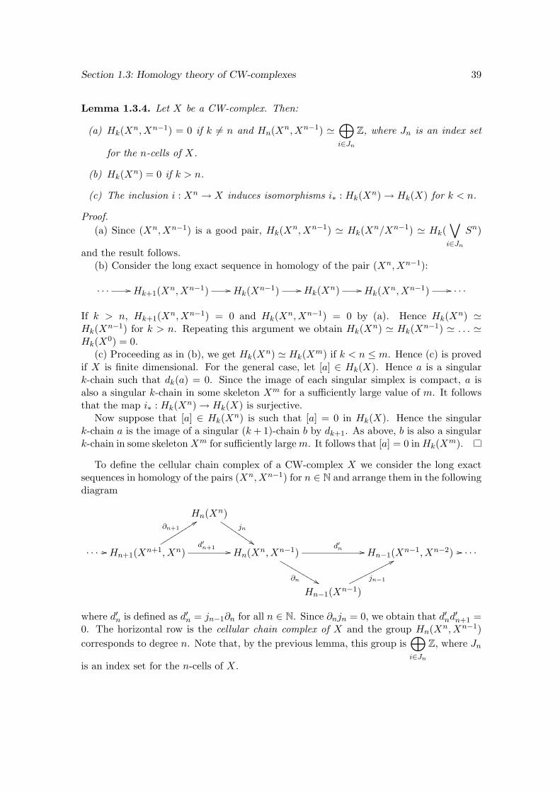
Section 1.3: Homology theory of CW-complexes 39
Lemma 1.3.4. Let X be a CW-complex. Then:
(a) Hk(Xn, Xn−1) = 0 if k 6= n and Hn(Xn, Xn−1) '⊕i∈Jn
Z, where Jn is an index set
for the n-cells of X.
(b) Hk(Xn) = 0 if k > n.
(c) The inclusion i : Xn → X induces isomorphisms i∗ : Hk(Xn) → Hk(X) for k < n.
Proof.(a) Since (Xn, Xn−1) is a good pair, Hk(Xn, Xn−1) ' Hk(Xn/Xn−1) ' Hk(
∨i∈Jn
Sn)
and the result follows.(b) Consider the long exact sequence in homology of the pair (Xn, Xn−1):
. . . // Hk+1(Xn, Xn−1) // Hk(Xn−1) // Hk(Xn) // Hk(Xn, Xn−1) // . . .
If k > n, Hk+1(Xn, Xn−1) = 0 and Hk(Xn, Xn−1) = 0 by (a). Hence Hk(Xn) 'Hk(Xn−1) for k > n. Repeating this argument we obtain Hk(Xn) ' Hk(Xn−1) ' . . . 'Hk(X0) = 0.
(c) Proceeding as in (b), we get Hk(Xn) ' Hk(Xm) if k < n ≤ m. Hence (c) is provedif X is finite dimensional. For the general case, let [a] ∈ Hk(X). Hence a is a singulark-chain such that dk(a) = 0. Since the image of each singular simplex is compact, a isalso a singular k-chain in some skeleton Xm for a sufficiently large value of m. It followsthat the map i∗ : Hk(Xn) → Hk(X) is surjective.
Now suppose that [a] ∈ Hk(Xn) is such that [a] = 0 in Hk(X). Hence the singulark-chain a is the image of a singular (k+ 1)-chain b by dk+1. As above, b is also a singulark-chain in some skeletonXm for sufficiently largem. It follows that [a] = 0 inHk(Xm).
To define the cellular chain complex of a CW-complex X we consider the long exactsequences in homology of the pairs (Xn, Xn−1) for n ∈ N and arrange them in the followingdiagram
Hn(Xn)jn
$$IIIIIIIII
. . . // Hn+1(Xn+1, Xn)
∂n+1
99ssssssssss d′n+1 // Hn(Xn, Xn−1)d′n //
∂n &&LLLLLLLLLLHn−1(Xn−1, Xn−2) // . . .
Hn−1(Xn−1)jn−1
77ooooooooooo
where d′n is defined as d′n = jn−1∂n for all n ∈ N. Since ∂njn = 0, we obtain that d′nd′n+1 =
0. The horizontal row is the cellular chain complex of X and the group Hn(Xn, Xn−1)corresponds to degree n. Note that, by the previous lemma, this group is
⊕i∈Jn
Z, where Jn
is an index set for the n-cells of X.
Section 1.3: Homology theory of CW-complexes 40
The cellular homology groups of X are defined as the homology groups of the cellularchain complex of X. As we shall see shortly, cellular homology coincides with singularhomology and the differentials d′n can be calculated in terms of the attaching maps ofthe cells. Hence, singular homology of CW-complexes can be computed directly from thecombinatorial structure of CW-complexes by means of cellular homology. Moreover, it isclear that the cellular chain complex is far more simple that the singular one.
Before going on, we will prove that cellular homology groups coincide with singularhomology ones. Consider the long exact sequence
. . . // Hn+1(Xn+1, Xn)∂n+1 // Hn(Xn) // Hn(Xn+1) // Hn(Xn+1, Xn) // . . .
By the previous lemma, Hn(Xn+1) ' Hn(X) and Hn(Xn+1, Xn) = 0. In consequence,Hn(X) ' Hn(Xn)/Im ∂n+1.
On the other hand, given n ∈ N we consider the exact sequence
. . . // Hn(Xn−1) // Hn(Xn)jn // Hn(Xn, Xn−1)
∂n // Hn−1(Xn−1) // . . .
By the previous lemma, Hn(Xn−1) = 0. Hence, jn is injective. Thus, the maps jn|Im ∂n+1 :Im ∂n+1 → Im (jn∂n+1) = Im (d′n+1) and jn : Hn(Xn) → Im jn = ker ∂n are isomor-phisms. Now, ker ∂n = ker d′n since jn−1 is injective. Then jn induces an isomorphismHn(Xn)/Im ∂n+1 ' ker d′n/Im (d′n+1). Hence, cellular homology groups coincide withsingular homology ones.
As mentioned before, the differentials d′n can be computed in terms of the attachingmaps of the cells as stated by the following proposition.
Proposition 1.3.5. Let X be a CW-complex. For each n ∈ N, let Jn be an index setfor the n-cells. We consider the cells enα, α ∈ Jn, as generators of the free abelian groupHn(Xn, Xn−1) '
⊕α∈Jn
Z. Then the differential d′n is defined by
d′n(enα) =
∑β∈Jn−1
deg(qn−1β gnα)en−1
β
where gαn is the attaching map of enα and qn−1β : Xn−1 → Sn−1 is the quotient map which
collapses Xn−1 −
en−1β to a point.
Note that the sum above has finite support since the image of gnα is compact and henceit intersects only a finite number of cells.
The proof of this proposition will not be given here. However, a generalization of thisresult will be proved in chapter 5.
We will give now some examples of application of the above results which will show theusefulness of cellular homology.
Examples 1.3.6.
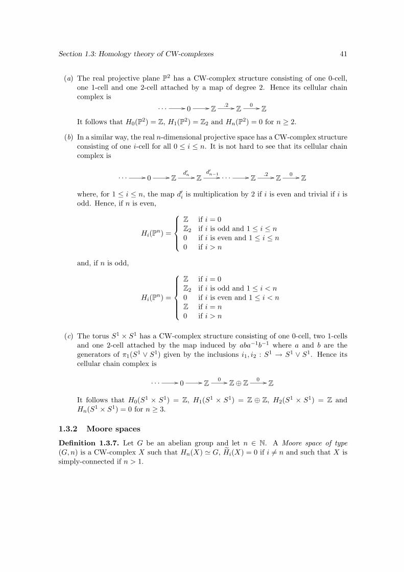
Section 1.3: Homology theory of CW-complexes 41
(a) The real projective plane P2 has a CW-complex structure consisting of one 0-cell,one 1-cell and one 2-cell attached by a map of degree 2. Hence its cellular chaincomplex is
. . . // 0 // Z .2 // Z 0 // Z
It follows that H0(P2) = Z, H1(P2) = Z2 and Hn(P2) = 0 for n ≥ 2.
(b) In a similar way, the real n-dimensional projective space has a CW-complex structureconsisting of one i-cell for all 0 ≤ i ≤ n. It is not hard to see that its cellular chaincomplex is
. . . // 0 // Zd′n // Z
d′n−1 // . . . // Z .2 // Z 0 // Z
where, for 1 ≤ i ≤ n, the map d′i is multiplication by 2 if i is even and trivial if i isodd. Hence, if n is even,
Hi(Pn) =
Z if i = 0Z2 if i is odd and 1 ≤ i ≤ n0 if i is even and 1 ≤ i ≤ n0 if i > n
and, if n is odd,
Hi(Pn) =
Z if i = 0Z2 if i is odd and 1 ≤ i < n0 if i is even and 1 ≤ i < nZ if i = n0 if i > n
(c) The torus S1 × S1 has a CW-complex structure consisting of one 0-cell, two 1-cellsand one 2-cell attached by the map induced by aba−1b−1 where a and b are thegenerators of π1(S1 ∨ S1) given by the inclusions i1, i2 : S1 → S1 ∨ S1. Hence itscellular chain complex is
. . . // 0 // Z 0 // Z⊕ Z 0 // Z
It follows that H0(S1 × S1) = Z, H1(S1 × S1) = Z ⊕ Z, H2(S1 × S1) = Z andHn(S1 × S1) = 0 for n ≥ 3.
1.3.2 Moore spaces
Definition 1.3.7. Let G be an abelian group and let n ∈ N. A Moore space of type(G,n) is a CW-complex X such that Hn(X) ' G, Hi(X) = 0 if i 6= n and such that X issimply-connected if n > 1.
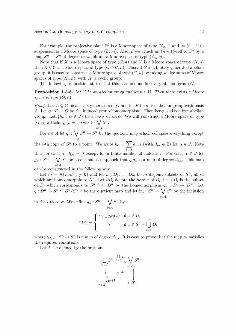
Section 1.3: Homology theory of CW-complexes 42
For example, the projective plane P2 is a Moore space of type (Z2, 1) and its (n− 1)thsuspension is a Moore space of type (Z2, n). Also, if we attach an (n+ 1)-cell to Sn by amap Sn → Sn of degree m we obtain a Moore space of type (Zm, n).
Note that if X is a Moore space of type (G,n) and Y is a Moore space of type (H,n)then X ∨Y is a Moore space of type (G⊕H,n). Thus, if G is a finitely generated abeliangroup, it is easy to construct a Moore space of type (G,n) by taking wedge sums of Moorespaces of type (Hi, n), with Hi a cyclic group.
The following proposition states that this can be done for every abelian group G.
Proposition 1.3.8. Let G be an abelian group and let n ∈ N. Then there exists a Moorespace of type (G,n).
Proof. Let A ⊆ G be a set of generators of G and let F be a free abelian group with basisA. Let φ : F → G be the induced group homomorphism. Then kerφ is also a free abeliangroup. Let hα : α ∈ J be a basis of kerφ. We will construct a Moore space of type(G,n) attaching (n+ 1)-cells to
∨i∈A
Sn.
For i ∈ A let qi :∨i∈A
Sn → Sn be the quotient map which collapses everything except
the i-th copy of Sn to a point. We write hα =∑i∈A
di,αi (with diα ∈ Z) for α ∈ J . Note
that for each α, di,α = 0 except for a finite number of indexes i. For each α ∈ J letgα : Sn →
∨i∈A
Sn be a continuous map such that qigα is a map of degree di,α. This map
can be constructed in the following way.Let m = #i ; di,α 6= 0 and let D1, D2, . . . , Dm be m disjoint subsets of Sn, all of
which are homeomorphic to Dn. Let ∂Di denote the border of Di, i.e. ∂Di is the subsetof Di which corresponds to Sn−1 ⊆ Dn by the homeomorphism ϕi : Di → Dn. Letq : Dn → Sn ' Dn/Sn−1 be the quotient map and let ini : Sn →
∨i∈A
Sn be the inclusion
in the i-th copy. We define gα : Sn →∨i∈A
Sn by
gi(x) =
γdi,α
qϕi(x) if x ∈ Di
∗ if x ∈ Sn −m⋃i=1
Di
where γdi,α: Sn → Sn is a map of degree di,α. It is easy to prove that the map gα satisfies
the required conditions.Let X be defined by the pushout
⊔α∈J
SnF
α∈Jgα
//
i
push
∨i∈A
Sn
tα∈J
Dn+1 // X
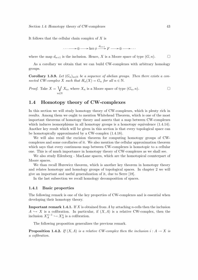
Section 1.4: Homotopy theory of CW-complexes 43
It follows that the cellular chain complex of X is
. . . // 0 // kerφdn+1 // F // 0 // . . .
where the map dn+1 is the inclusion. Hence, X is a Moore space of type (G,n).
As a corollary we obtain that we can build CW-complexes with arbitrary homologygroups.
Corollary 1.3.9. Let (Gn)n∈N be a sequence of abelian groups. Then there exists a con-nected CW-complex X such that Hn(X) = Gn for all n ∈ N.
Proof. Take X =∨n∈N
Xn, where Xn is a Moore space of type (Gn, n).
1.4 Homotopy theory of CW-complexes
In this section we will study homotopy theory of CW-complexes, which is plenty rich inresults. Among them we ought to mention Whitehead Theorem, which is one of the mostimportant theorems of homotopy theory and asserts that a map between CW-complexeswhich induces isomorphisms in all homotopy groups is a homotopy equivalence (1.4.14).Another key result which will be given in this section is that every topological space canbe homotopically approximated by a CW-complex (1.4.18).
We will also recall the excision theorem for computing homotopy groups of CW-complexes and some corollaries of it. We also mention the cellular approximation theoremwhich says that every continuous map between CW-complexes is homotopic to a cellularone. This is of much importance in homotopy theory of CW-complexes as we shall see.
We also study Eilenberg - MacLane spaces, which are the homotopical counterpart ofMoore spaces.
We than recall Hurewicz theorem, which is another key theorem in homotopy theoryand relates homotopy and homology groups of topological spaces. In chapter 2 we willgive an important and useful generalization of it, due to Serre [18].
In the last subsection we recall homology decomposition of spaces.
1.4.1 Basic properties
The following remark is one of the key properties of CW-complexes and is essential whendeveloping their homotopy theory.
Important remark 1.4.1. IfX is obtained from A by attaching n-cells then the inclusionA → X is a cofibration. In particular, if (X,A) is a relative CW-complex, then theinclusion Xn−1
A → XnA is a cofibration.
The following proposition generalizes the previous remark.
Proposition 1.4.2. If (X,A) is a relative CW-complex then the inclusion i : A → X isa cofibration.
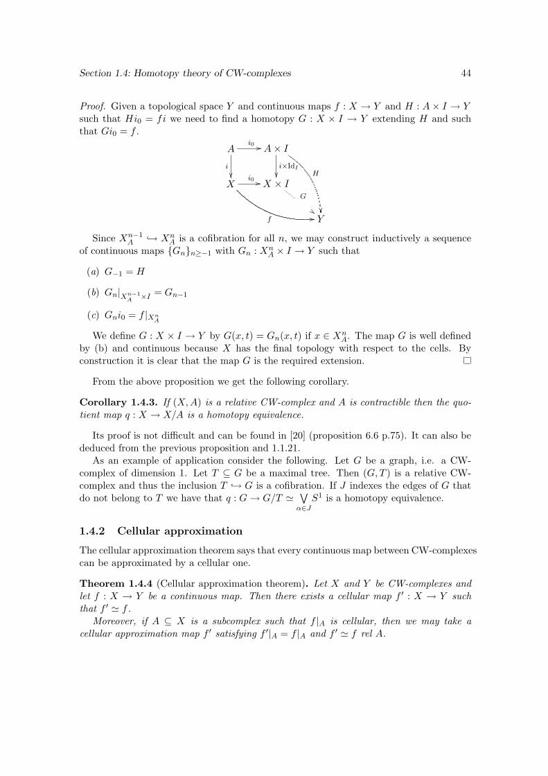
Section 1.4: Homotopy theory of CW-complexes 44
Proof. Given a topological space Y and continuous maps f : X → Y and H : A× I → Ysuch that Hi0 = fi we need to find a homotopy G : X × I → Y extending H and suchthat Gi0 = f .
Ai0 //
i
A× I
i×IdI
H
Xi0 //
f 00
X × IG
##Y
Since Xn−1A → Xn
A is a cofibration for all n, we may construct inductively a sequenceof continuous maps Gnn≥−1 with Gn : Xn
A × I → Y such that
(a) G−1 = H
(b) Gn|Xn−1A ×I = Gn−1
(c) Gni0 = f |XnA
We define G : X × I → Y by G(x, t) = Gn(x, t) if x ∈ XnA. The map G is well defined
by (b) and continuous because X has the final topology with respect to the cells. Byconstruction it is clear that the map G is the required extension.
From the above proposition we get the following corollary.
Corollary 1.4.3. If (X,A) is a relative CW-complex and A is contractible then the quo-tient map q : X → X/A is a homotopy equivalence.
Its proof is not difficult and can be found in [20] (proposition 6.6 p.75). It can also bededuced from the previous proposition and 1.1.21.
As an example of application consider the following. Let G be a graph, i.e. a CW-complex of dimension 1. Let T ⊆ G be a maximal tree. Then (G,T ) is a relative CW-complex and thus the inclusion T → G is a cofibration. If J indexes the edges of G thatdo not belong to T we have that q : G→ G/T '
∨α∈J
S1 is a homotopy equivalence.
1.4.2 Cellular approximation
The cellular approximation theorem says that every continuous map between CW-complexescan be approximated by a cellular one.
Theorem 1.4.4 (Cellular approximation theorem). Let X and Y be CW-complexes andlet f : X → Y be a continuous map. Then there exists a cellular map f ′ : X → Y suchthat f ′ ' f .
Moreover, if A ⊆ X is a subcomplex such that f |A is cellular, then we may take acellular approximation map f ′ satisfying f ′|A = f |A and f ′ ' f rel A.
Section 1.4: Homotopy theory of CW-complexes 45
Its proof can be found in [20].We will see now some important applications of this teorem. For the first of them we
need the following classical lemma about relative homotopy groups.
Lemma 1.4.5. Let (X,x0) be a pointed topological space and let A ⊆ X be a subspacesuch that x0 ∈ A. Let f : (Dn, Sn−1) → (X,A) be a continuous map. Then the followingare equivalent.
i) There exists a base point preserving homotopy H : (Dn× I, Sn−1× I) → (X,A) suchthat Hi0 = f , Hi1(x) = x0 ∀x ∈ Dn.
ii) There exists a (base point preserving) homotopy G : Dn × I → X, relative to Sn−1,such that Gi0 = f , Gi1(Dn) ⊆ A.
iii) There exists a (base point preserving) homotopy G : Dn×I → X, such that Gi0 = f ,Gi1(Dn) ⊆ A.
We omit the proof which is not difficult. Besides, we will give later a generalization ofthis result (4.1.5). As an immediate application we obtain the following corollary.
Corollary 1.4.6. Let (X,A, x0) be a pointed topological pair (i.e. (X,x0) is a pointedtopological space and A ⊆ X is a subspace such that x0 ∈ A) and let f : (Dn, Sn−1, s0) →(X,A, x0) be a continuous map. Then [f ] = 0 in πn(X,A) if and only if f is homotopicrelative to Sn−1 to a map g such that g(Dn) ⊆ A.
With this results at hand, we are able to give the first application of the cellularapproximation theorem.
Corollary 1.4.7. If X is a CW-complex, then the topological pair (X,Xn) is n-connected,i.e, πr(X,Xn) = 0 for all r ≤ n, or equivalently, the morphism i∗ : πr(Xn) → πr(X),induced by the inclusion, is an isomorphism for r < n and an epimorphism for r = n.
Proof. Let r ≤ n and let [f ] ∈ πr(X,Xn). We can take any 0-cell as base point forπr(X,Xn) since every point can be joined to a 0-cell by a continuous path. Hence, wemay suppose that f sends the base point of Dr to a 0-cell.
We consider in Sr−1 the cellular structure which consists of one 0-cell and one (r− 1)-cell. Note that f |Sr−1 is cellular. Thus, by the cellular approximation theorem there existsa cellular map f ′ : Dr → X such that f ′|Sr−1 = f |Sr−1 and f ′ ' f rel Sr−1.
Since f ′ is celular and r < n then Im f ′ ⊆ Xn. Hence f is homotopic (relative to Sr−1)to a map f ′ with Im f ′ ⊆ Xn. Thus, [f ] = 0 in πr(X,Xn) by the corollary above.
Corollary 1.4.8. πr(Sn) = 0 for r < n.
Proof. Let r < n. We consider in Sr the cellular structure que which consists of one 0-celland one r-cell, and in Sn the analogous structure. Let [f ] ∈ πr(Sn). By the cellularapproximation theorem, there exists a cellular map f ′ : Sr → Sn, such that f ′ ' f rel ∗(where ∗ is the 0-cell). But then f ′(Sr) ⊆ (Sn)r = ∗, i. e. f ′ is constant.
Thus, [f ] = 0.
Section 1.4: Homotopy theory of CW-complexes 46
We give now two variations of the cellular approximation theorem: for CW-pairs andfor relative CW-complexes.
Proposition 1.4.9 (Cellular approximation theorem for CW-pairs). Let f : (X,A) →(Y,B) be a continuous map between CW-pairs. Then there exists a cellular map g :(X,A) → (Y,B) such that f ' g as maps between topological pairs.
Proposition 1.4.10 (Cellular approximation theorem for relative CW-complexes). Letf : (X,A) → (Y,B) be a continuous map between relative CW-complexes. Then thereexists a cellular map g : (X,A) → (Y,B) (i.e. g(Xn
A) ⊆ Y nB for all n) such that f ' g
relative to A.
As a corollary we get the following theorem, which is analogous to 1.4.7.
Corollary 1.4.11. Let (X,A) be a relative CW-complex and let n ∈ N0. If (X,A) has nocells of dimension less than or equal to n, then the topological pair (X,A) is n-connected.
1.4.3 Whitehead theorem
Whitehead’s theorem is one of the most important theorems of the homotopy theory ofclassical CW-complexes. The proof we will give here will use the cellular approximationtheorem. A bit more elementary proof, without using the cellular approximation theoremcan be found in [20] and a generalization of this proof is given in chapter 4 of this thesis,in our generalization of Whitehead theorem (4.2.4).
For the proof of Whitehead theorem we will need the following lemma, interesting forits own sake.
Lemma 1.4.12. Let (X,A) be a relative CW-complex and let (Y,B) be a topologicalpair with B 6= ∅. Suppose that for all n ∈ N0 such that there exists at least one n-cellin X − A we have that πn(Y,B, b0) = 0 for all b0 ∈ B. Then every continuous mapf : (X,A) → (Y,B) is homotopic relative to A to a map g such that g(X) ⊆ B.
Note that this lemma generalizes 1.4.6.In particular if dim(X,A) = n (resp. dim(X,A) = ∞) and (Y,B) is n-connected (resp.
πn(Y,B) = 0 for all n ∈ N) then the hypothesis of the lemma are satisfied.
Proof. By induction, suppose h : X → Y is a continuous map such that h(Xn−1A ) ⊆ B.
Let en ∈ XnA and let ϕ : (Dn, Sn−1) → (Xn
A, Xn−1A ) be the characteristic map of en. Then
hϕ : (Dn, Sn−1) → (Y,B). Since πn(Y,B) = 0 then there exists a map ψ such that hϕ ' ψrel Sn−1 and ψ(Dn) ⊆ B.
Hence, there exists a continuous map h′ : Xn−1A ∪ en → Y such that h′(Xn−1
A ∪ en) ⊆ Band h|Xn−1
A ∪en ' h′ rel Xn−1A .
Doing this for all cells of dimension n we obtain a continuous map h : XnA → Y with
h(XnA) ⊆ B and a homotopy H : h|Xn
A' h rel Xn−1
A . Since the inclusion i : XnA → X is a
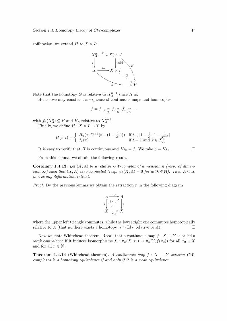
Section 1.4: Homotopy theory of CW-complexes 47
cofibration, we extend H to X × I:
XnA
i0 //
i
XnA × I
i×IdI
H
Xi0 //
h 00
X × IG
##Y
Note that the homotopy G is relative to Xn−1A since H is.
Hence, we may construct a sequence of continuous maps and homotopies
f = f−1 'H0
f0 'H1
f1 'H2
. . .
with fn(XnA) ⊆ B and Hn relative to Xn−1
A .Finally, we define H : X × I → Y by
H(x, t) =Hn(x, 2n+1(t− (1− 1
2n ))) if t ∈ [1− 12n , 1− 1
2n+1 ]fn(x) if t = 1 and x ∈ Xn
A
It is easy to verify that H is continuous and Hi0 = f . We take g = Hi1.
From this lemma, we obtain the following result.
Corollary 1.4.13. Let (X,A) be a relative CW-complex of dimension n (resp. of dimen-sion ∞) such that (X,A) is n-connected (resp. πk(X,A) = 0 for all k ∈ N). Then A ⊆ Xis a strong deformation retract.
Proof. By the previous lemma we obtain the retraction r in the following diagram
AIdA //
i
A
i
XIdX
//
∃r>>
X
where the upper left triangle commutes, while the lower right one commutes homotopicallyrelative to A (that is, there exists a homotopy ir ' IdX relative to A).
Now we state Whitehead theorem. Recall that a continuous map f : X → Y is called aweak equivalence if it induces isomorphisms f∗ : πn(X,x0) → πn(Y, f(x0)) for all x0 ∈ Xand for all n ∈ N0.
Theorem 1.4.14 (Whitehead theorem). A continuous map f : X → Y between CW-complexes is a homotopy equivalence if and only if it is a weak equivalence.
Section 1.4: Homotopy theory of CW-complexes 48
Proof. The first implication holds for every topological space (see [19]).For the converse note that if f is the inclusion of a subcomplex in a CW-complex, the
result follows from the previous corollary.For the general case, let f : X → Y be any continuous map. By the cellular approxi-
mation theorem there exists a cellular map f ′ : X → Y such that f ′ ' f . Note that f ′ isa weak equivalence since f is.
By 1.2.29, Zf ′ is a CW-complex and X ⊆ Zf ′ is subcomplex. We have a commutativediagram
Xf ′ //
j
Y
i~~
Zf ′
r>>
where j and i are inclusion maps and where r : Zf ′ → Y is the standard strong deformationretraction.
Since f ′ : X → Y is a weak equivalence, then j : X → Zf ′ is a weak equivalence. Bythe previous case, j is a homotopy equivalence. Then f ′ = rj is a homotopy equivalenceand since f ' f ′, then f is a homotopy equivalence.
1.4.4 CW-approximations
We will now take study CW-approximations, that is, given a topological space X we wantto find a CW-complex which ‘homotopically approximates’ the space X. More precisely,
Definition 1.4.15. Let X be a topological space. A CW-approximation of X is a CW-complex Z together with a weak equivalence f : Z → X.
We will prove that every topological spaceX admits a CW-approximation as a corollaryof a stronger result, for which we need the following definition.
Definition 1.4.16. Let (X,A) be a topological pair where A ⊆ X is a non-empty CW-complex and let n ∈ N0. An n-connected CW-model of (X,A) (or simply an n-model of(X,A)) is a CW-pair (Z,A) together with a continuous map f : Z → X such that f |A = Idand such that
(a) The pair (Z,A) is n-connected.
(b) For every z0 ∈ Z the morphism f∗ : πr(Z, z0) → πr(X, f(z0)) is an isomorphism forall r > n and a monomorphism for r = n.
Note that an n-model (Z,A) of (X,A) is a kind of ‘homotopic mixture’ between A andX. If i : A→ Z and j : A→ X are the inclusion maps and f : Z → X is as in the previousdefinition, then i∗ : πr(A) → πr(Z) is a isomorphism for all r < n and f∗ : πr(Z) → πr(X)is a isomorphism for all r > n.
Moreover, i∗ : πn(A) → πn(Z) is an epimorphism and f∗ : πn(Z) → πn(X) is amonomorphism and since fi = j, then f∗i∗ = j∗. Hence, in some way πn(Z) can bethought as the image of πn(A) in πn(X).
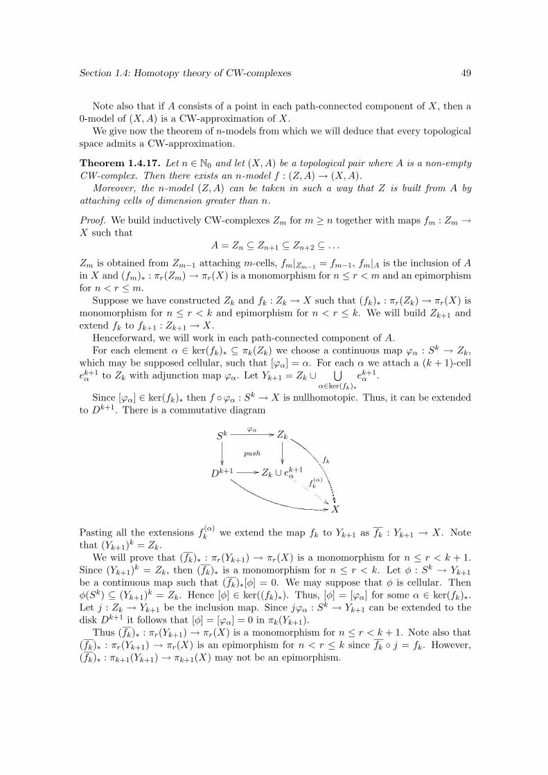
Section 1.4: Homotopy theory of CW-complexes 49
Note also that if A consists of a point in each path-connected component of X, then a0-model of (X,A) is a CW-approximation of X.
We give now the theorem of n-models from which we will deduce that every topologicalspace admits a CW-approximation.
Theorem 1.4.17. Let n ∈ N0 and let (X,A) be a topological pair where A is a non-emptyCW-complex. Then there exists an n-model f : (Z,A) → (X,A).
Moreover, the n-model (Z,A) can be taken in such a way that Z is built from A byattaching cells of dimension greater than n.
Proof. We build inductively CW-complexes Zm for m ≥ n together with maps fm : Zm →X such that
A = Zn ⊆ Zn+1 ⊆ Zn+2 ⊆ . . .
Zm is obtained from Zm−1 attaching m-cells, fm|Zm−1 = fm−1, fm|A is the inclusion of Ain X and (fm)∗ : πr(Zm) → πr(X) is a monomorphism for n ≤ r < m and an epimorphismfor n < r ≤ m.
Suppose we have constructed Zk and fk : Zk → X such that (fk)∗ : πr(Zk) → πr(X) ismonomorphism for n ≤ r < k and epimorphism for n < r ≤ k. We will build Zk+1 andextend fk to fk+1 : Zk+1 → X.
Henceforward, we will work in each path-connected component of A.For each element α ∈ ker(fk)∗ ⊆ πk(Zk) we choose a continuous map ϕα : Sk → Zk,
which may be supposed cellular, such that [ϕα] = α. For each α we attach a (k + 1)-cellek+1α to Zk with adjunction map ϕα. Let Yk+1 = Zk ∪
⋃α∈ker(fk)∗
ek+1α .
Since [ϕα] ∈ ker(fk)∗ then f ϕα : Sk → X is nullhomotopic. Thus, it can be extendedto Dk+1. There is a commutative diagram
Skϕα //
push
Zk
fk
Dk+1 //
00
Zk ∪ ek+1α
f(α)k
$$X
Pasting all the extensions f (α)k we extend the map fk to Yk+1 as fk : Yk+1 → X. Note
that (Yk+1)k = Zk.We will prove that (fk)∗ : πr(Yk+1) → πr(X) is a monomorphism for n ≤ r < k + 1.
Since (Yk+1)k = Zk, then (fk)∗ is a monomorphism for n ≤ r < k. Let φ : Sk → Yk+1
be a continuous map such that (fk)∗[φ] = 0. We may suppose that φ is cellular. Thenφ(Sk) ⊆ (Yk+1)k = Zk. Hence [φ] ∈ ker((fk)∗). Thus, [φ] = [ϕα] for some α ∈ ker(fk)∗.Let j : Zk → Yk+1 be the inclusion map. Since jϕα : Sk → Yk+1 can be extended to thedisk Dk+1 it follows that [φ] = [ϕα] = 0 in πk(Yk+1).
Thus (fk)∗ : πr(Yk+1) → πr(X) is a monomorphism for n ≤ r < k + 1. Note also that(fk)∗ : πr(Yk+1) → πr(X) is an epimorphism for n < r ≤ k since fk j = fk. However,(fk)∗ : πk+1(Yk+1) → πk+1(X) may not be an epimorphism.
Section 1.4: Homotopy theory of CW-complexes 50
For each β ∈ πk+1(X) we take a continuous map ϕβ : Sk+1 → X such that [ϕβ] = β.Let Zk+1 = Yk+1 ∨
∨β∈πk+1(X)
Sk+1 and fk+1 : Zk+1 → X be defined by fk+1|Yk+1= fk and
fk+1|Sk+1β
= ϕβ.
Note that (Zk+1)k = (Yk+1)k = Zk. Hence πr(Yk+1) = πr(Zk+1) = πr(Zk) for n ≤ r <k. Thus (fk+1)∗ : πr(Zm) → πr(X) is a monomorphism for n ≤ r < k and an epimorphismfor n < r < k.
By construction, (fk+1)∗ : πk+1(Zk+1) → πk+1(X) is an epimorphism. Indeed, ifiβ : Sk+1 → Zk+1 denotes the inclusion in the β-th copy of Sk+1 then (fk+1)∗([iβ]) =[fk+1iβ] = [ϕβ].
We will see now that (fk+1)∗ : πk(Zk+1) → πk(X) is an isomorphism. Since Yk+1 ⊆Zk+1 is a retract (with retraction r : Zk+1 → Yk+1 sending
∨β∈πk+1(X)
Sk+1 to a point) then
ri = IdYk+1, where i : Yk+1 → Zk+1 is the inclusion. Then, r∗i∗ = Id, and it follows
that i∗ : πk(Yk+1) → πk(Zk+1) is a monomorphism. Moreover, by cellular approximation,i∗ : πk(Yk+1) → πk(Zk+1) is an epimorphism. Then, it is an isomorphism. Since fk+1i = fkit follows that (fk+1)∗ : πk(Zk+1) → πk(X) is an isomorphism.
We take Z =⋃k≥n
Zk and f : Z → X defined by f |Zk= fk. It follows that f : (Z,A) →
(X,A) is an n-model of (X,A).
As said before, we obtain as a corollary the following theorem.
Theorem 1.4.18. Let X be a topological space. Then there exists a CW-approximationfor X.
Proof. We take A consisting of a point in each path-connected component of X. Letf : (Z,A) → (X,A) be a 0-connected model of (X,A). The map f : Z → X is a CW-approximation for X.
There is also a CW-approximation theorem for topological pairs.
Theorem 1.4.19. Let (X,A) be a topological pair. Then there exists a CW-pair (Z,B)and a continuous map f : (Z,B) → (X,A) such that f∗ : πn(B) → πn(A), f∗ : πn(Z) →πn(X) and f∗ : πn(Z,B) → πn(X,A) are isomorphisms for all n.
Proof. Let g : B → A be a CW-approximation for A. Let in : A → X be the inclusionmap and let α : (Z,B) → (Zing, B) be a 0-connected CW-model for (Zing, B). Letr : Zing → B be the standard strong deformation retraction and let f = rα. It followsthat f |B = g and that f∗ : πn(B) → πn(A) and f∗ : πn(Z) → πn(X) are isomorphisms forall n ∈ N0. Thus, from the five-lemma, f∗ : πn(Z,B) → πn(X,A) is also an isomorphismfor all n.
Another important consequence of 1.4.17 is the following proposition.
Proposition 1.4.20. If (X,A) is an n-connected relative CW-complex, then there existsa relative CW-complex (Z,A) such that (X,A) is homotopy equivalent to (Z,A) relativeto A and (Z,A) has no cells of dimension less than n+ 1.
Section 1.4: Homotopy theory of CW-complexes 51
1.4.5 More homotopical properties
In a similar way as in homology, for homotopy groups of CW-complexes there is an excisiontheorem. However, it has a dimensional restriction.
Theorem 1.4.21 (Homotopy excision theorem). Let X be a topological space and let Aand B be subspaces of X such that X = A ∪ B, (A,A ∩ B) is an n-connected relativeCW-complex with n ≥ 1 and (B,A ∩ B) is an m-connected relative CW-complex. Letj : (A,A ∩ B) → (X,B) be the inclusion. Then j∗ : πr(A,A ∩ B) → πr(X,B) is anisomorphism for 1 ≤ r < n+m and an epimorphism for r = m+ n.
We will not give the proof here as it is quite technical and the ideas do not shed anylight on our work. However, it is an important result and shows the difference in difficultybetween dealing with homology groups and with homotopy groups.
As a corollary, we obtain the following proposition which is a refined version of 1.4.3.
Proposition 1.4.22. Let (X,A) be a CW-pair such that A is m-connected and (X,A) isn-connected with n ≥ 1. Let q : (X,A) → (X/A, ∗) be the quotient map. Then the inducedmap q∗ : πr(X,A) → πr(X/A) is an isomorphism for 2 ≤ r ≤ m+ n and an epimorphismfor r = m+ n+ 1.
Another important theorem concerning homotopy theory of CW-complexes is Freud-hental suspension theorem. Recall that for homology groups one always has an isomor-phism Hn(X) ' Hn+1(ΣX). This is not the case for homotopy groups, where someconditions must be imposed.
Theorem 1.4.23 (Freudhental suspension theorem). Let X be an n-connected CW-complex, with n ≥ 0. Then Σ : πr(X) → πr+1(ΣX) is an isomorphism for 1 ≤ r ≤ 2n andan epimorphism for r = 2n+ 1.
Using that π2(S2) = Z and Freudhental suspension theorem we obtain the following.
Corollary 1.4.24. πn(Sn) = Z for all n ∈ N.
Proof. Since Sn is (n − 1)-connected, Freudhental suspension theorem gives an isomor-phism Σ : πn(Sn) → πn+1(Sn+1) if 1 ≤ n ≤ 2n − 2 (i.e. if n ≥ 2) and an epimorphism ifn = 2n− 1 (i.e. if n = 1).
The fact that π2(S2) = Z will be proved in next chapter (p. 64) as an application ofthe exact sequence of homotopy groups associated to a fibration.
We define now the stable homotopy groups of a space X.
Definition 1.4.25. Let X be a topological space and let n ∈ N0. We define the n-thstable homotopy group of X as πst
n (X) = colimk
πn+k(ΣkX).
If X is a CW-complex then ΣkX is (k−1)-connected. From the Freudhental suspensiontheorem it follows that πn+k(ΣkX) ' πn+k+1(Σk+1X) if n+ k ≤ 2(k − 1) or equivalentlyif k ≥ n + 2. Then the groups πn+k(ΣkX), k ∈ N, stabilize for k sufficiently large andπstn (X) ' πn+k(ΣkX) for all k ≥ n+ 2.
Section 1.4: Homotopy theory of CW-complexes 52
Continuing with our comparison between homology and homotopy properties, we willanalize now the analogous in homotopy groups of the wedge axiom for homology. Asbefore, some hypothesis on the degrees of connectedness of the spaces are needed so thatthe wedge axiom holds.
Proposition 1.4.26. Let X be an n-connected CW-complex and let Y be an m-connectedCW-complex. Let iX : X → X ∨ Y and iY : Y → X ∨ Y be the inclusion maps. Supposethat X or Y is locally compact. Then the induced map (iX)∗ ⊕ (iY )∗ : πr(X) ⊕ πr(Y ) →πr(X ∨ Y ) is an isomorphism for 2 ≤ r ≤ n+m.
Proof. Since X or Y is locally compact the space X × Y with the product topology is aCW-complex with the product CW-structure. Let x0 and y0 be the base points of X andY respectively. We know that X ∨ Y is homeomorphic to X × y0 ∪ x0 × Y ⊆ X × Y .Hence we will consider X ∨ Y as a subspace of X × Y .
Since X is an n-connected CW-complex we may suppose that Xn = x0. In a similarway, we may suppose that Y m = y0. Then (X × Y,X ∨ Y )n+m+1 = X ∨ Y . Letj : X ∨ Y → X × Y be the inclusion map. From the long exact sequence of homotopygroups associated to the pair (X × Y,X ∨ Y ) we obtain that j∗ : πr(X ∨ Y ) → πr(X × Y )is an isomorphism for 1 ≤ r ≤ n+m.
Let pX : X×Y → X and pY : X×Y → Y be the projections. Clearly, the induced map((pX)∗, (pY )∗) : πr(X×Y ) → πr(X)×πr(Y ) is an isomorphism for all r. But πr(X)×πr(Y )is isomorphic to πr(X) ⊕ πr(Y ) for r ≥ 2, so we consider ((pX)∗, (pY )∗) : πr(X × Y ) →πr(X)⊕ πr(Y ) for r ≥ 2.
Since ((pX)∗, (pY )∗) j∗ ((iX)∗ ⊕ (iY )∗) is the identity map of πr(X) ⊕ πr(Y ), theresult follows.
As a corollary we obtain the following
Corollary 1.4.27. Let I be an index set. For α ∈ I, let iα : Sn →∨i∈I
Sn denote the
inclusion in the α-th copy of Sn. Then the induced morphism⊕α∈I
(iα)∗ :⊕α∈I
πn(Sn) →
πn(∨i∈I
Sn) is an isomorphism for n ≥ 2.
The proof follows easily from the previous proposition if I is a finite set. For the generalcase the result is proved by a standard compactness argument.
Recall that π1(∨α∈I
Sn) is the free group generated by [iα] : α ∈ I.
1.4.6 Eilenberg - MacLane spaces
Definition 1.4.28. Let n ∈ N and let G be a group, which we require to be abelian ifn ≥ 2. An Eilenberg - MacLane space of type (G,n) is a path-connected CW-complex Xsuch that πn(X) ' G and πi(X) = 0 if i 6= n.
For example, the circle S1 is an Eilenberg - MacLane space of type (Z, 1). Despite thissimple example, Eilenberg - MacLane spaces are in general much more complicated than
Section 1.4: Homotopy theory of CW-complexes 53
Moore spaces. We will show now how to construct arbitrary Eilenberg - MacLane spaces.In contrast to the construction of Moore spaces, we will need to attach an infinite numberof cells of different dimensions.
In order to make the key idea more explicit, we prove first the following lemma.
Lemma 1.4.29. Let X be a path-connected CW-complex and let n ∈ N, n ≥ 2. Thenthere exists a CW-complex X ′ such that πi(X) ' πi(X ′) for i < n, πn(X ′) = 0 and X ′ isobtained from X by attaching (n+ 1)-cells.
Proof. Let φα : α ∈ J be a set of generators of πn(X). For each α ∈ J let gα : Sn → Xbe a continuous map such that [gα] = φα. By cellular approximation, we may supposethat gα is a cellular map. Let X ′ be the CW-complex obtained by attaching (n+ 1)-cellsto X by the maps gα, α ∈ J .
Now we will see that X ′ satisfies the required conditions. Consider the long exactsequence in homotopy groups associated to the pair (X ′, X):
. . . // πr(X) // πr(X ′) // πr(X ′, X) // πr−1(X) // . . .
Note that πr(X ′, X) = 0 for r ≤ n. Indeed, let [α] ∈ πr(X ′, X). Then α : (Dr, Sr−1) →(X ′, X). By the cellular approximation theorem for CW-pairs α is homotopic (as mapsbetween pairs) to a cellular map β. But since r ≤ n, the image of β must be contained inX. Thus, by 1.4.6, [α] = 0.
Hence, from the long exact sequence above it follows that the inclusion i∗ inducesisomorphisms i∗ : πr(X) → πr(X ′) for r < n and an epimorphism i∗ : πn(X) → πn(X ′).Now, note that i∗([gα]) = 0 in πn(X ′) since gα can be extended to Dn (the extension is thecharacteristic map of the (n+ 1)-cell attached). Since generators of πn(X) are mapped to0 by the epimorphism i∗ : πn(X) → πn(X ′), it follows that πn(X ′) = 0.
Proposition 1.4.30. Let n ∈ N and let G be a group if n = 1 and an abelian group ifn ≥ 2. Then there exists an Eilenberg - MacLane space of type (G,n).
Proof. We prove the case n ≥ 2. The case n = 1 is similar and can be found in [8](corollary 1.28).
Let gi : i ∈ I ⊆ G be a set of generators of G and let F be a free abelian group withbasis gi : i ∈ I. Let φ : F → G be the induced group homomorphism. Then kerφ is alsoa free abelian group. Let hα : α ∈ J be a basis of kerφ. We will construct an Eilenberg -MacLane space of type (G,n) attaching cells to
∨i∈I
Sn. Note that πn(∨i∈I
Sn) =⊕i∈I
Z = F .
For each α ∈ J let gα : Sn →∨i∈I
Sn be a continuous map such that [gα] ∈ πn(∨i∈I
Sn)
corresponds to hα ∈ F .
Section 1.4: Homotopy theory of CW-complexes 54
Let Xn =∨i∈I
Sn and let Xn+1 be defined by the pushout
⊔α∈J
SnF
α∈Jgα
//
i
push
∨i∈I
Sn
⊔α∈J
Dn+1 // Xn+1
Consider the following diagram
πn+1(Xn+1, Xn) ∂ //
ϕ '
πn(Xn)i∗ //
β '
πn(Xn+1) // πn(Xn+1, Xn) = 0
kerφinc
// Fφ // G // 0
where the isomorphism ϕ is given by the composition
πn+1(Xn+1, Xn) ' πn+1(Xn+1/Xn) ' πn+1(∨α∈J
Sn) ' kerφ.
Hence, the characteristic maps fα : α ∈ J form a basis of πn+1(Xn+1, Xn) since theycorrespond to the inclusions iα : Sn →
∨α∈J
Sn. Note that the above square commutes since
∂([fα]) = [gα] = β−1(hα).Thus, πn(Xn+1) ' G. And πr(Xn+1) ' πr(Xn) = 0 for r < n, since Xn+1 is obtained
from Xn by attaching (n+ 1)-cells.Applying the previous lemma, we build inductively a sequence of CW-complexes (Xm)m≥n+2
such that πn(Xm) ' G, πr(Xm) = 0 for r ≤ m−1, r 6= n and Xm is obtained from Xm−1
by attaching m-cells.We take X = colimXn. Since πr(X) ' πr(Xr+1) for all r ∈ N, it follows that X is an
Eilenberg - MacLane space of type (G,n).
Corollary 1.4.31. Let (Gn)n∈N be a sequence of abelian groups. Then there exists apath-connected CW-complex X such that πn(X) = Gn for all n ∈ N.
Proof. Take X =∏n∈N
Xn, where Xn is an Eilenberg - MacLane space of type (Gn, n).
An important result is that, fixed G and n, Eilenberg - MacLane spaces of type (G,n)are unique up to homotopy equivalence.
Proposition 1.4.32. The homotopy type of an Eilenberg - MacLane space of type (G,n)is uniquely determined by G and n.
The proof is not difficult but technical and we omit it.
Section 1.4: Homotopy theory of CW-complexes 55
1.4.7 Hurewicz theorem
As it was mentioned earlier, Hurewicz theorem is one of the most important theorems ofhomotopy theory. It connects homotopy theory with homology theory via a map knownas the Hurewicz map, which we recall right now.
Let X be a topological space and let 1 ∈ Hn(Sn) ' Z be a fixed generator of Hn(Sn).We define the Hurewicz map h : πn(X) → Hn(X) by h([α]) = α∗(1).
A relative version of the Hurewicz map can also be defined and this is done as follows.Let (X,A) be a topological pair and let 1 ∈ Hn(Dn, Sn−1) ' Z be a fixed generator ofHn(Dn, Sn−1). We define h : πn(X) → Hn(X) by h([α]) = α∗(1).
Before stating Hurewicz theorem we give a technical lemma which will be needed forthe proof of the theorem.
Lemma 1.4.33. Let n ∈ N and let X be a space obtained by attaching (n + 1)-cells to∨α∈I
Sn. Let Y be a path connected topological space and let ϕ : πn(X) → πn(Y ) be a group
homomorphism. Then there exists a continuous map f : X → Y such that the inducedmap f∗ : πn(X) → πn(Y ) coincides with ϕ.
Proof. Let iα : Sn → X denote the composition of the inclusions Sn →∨i∈I
Sn and∨i∈I
Sn → X, where the first one is the inclusion in the α-th copy, and let ηα : Sn → Y be
a continuous map such that [ηα] = ϕ([iα]).We define η :
∨α∈I
Sn → Y by η = +α∈I
ηα. Then η∗([iα]) = [η iα] = [ηα] = ϕ([iα]) for all
α ∈ I. Since iα : α ∈ I is a set of generators of πn(∨i∈I
Sn) we obtain that η(γ) = ϕ(γ)
for all γ ∈ πn(∨i∈I
Sn).
Let J be an index set for the (n + 1)-cells of X. For each β ∈ J let gβ : Sn →∨α∈I
Sn
be the attaching map of the cell en+1β . Note that gβ is nullhomotopic in X since the
corresponding characteristic map is an extension of gβ : Sn → X to the cone CSn.Thus, [η gβ] = η∗([gβ]) = ψ([gβ]) = 0 since [gβ] = 0 in πn(X). Hence, there exists
continuous maps ϕβ : Dn+1 → Y such that φβ|Sn = η gβ.We define f : X → Y as the dotted arrow in the diagram
tβ∈J
Snt
β∈Jgβ
//
i
push
∨α∈I
Sn
inc
η
tβ∈J
Dn+1
tβ∈J
fβ
//
tβ∈J
φβ //
Xf
!!Y
Section 1.4: Homotopy theory of CW-complexes 56
Since the inclusion inc : Xn → X induces an epimorphism inc∗ : πn(Xn) → πn(X) by1.4.5, then inc∗([iα]) : α ∈ I is a set of generators of πn(X). Note that f∗(inc∗([iα])) =η∗([iα]) = ϕ([iα]). Hence, f∗ = ϕ.
Theorem 1.4.34 (Hurewicz theorem). Let n ∈ N, n ≥ 2 and let X be an (n−1)-connectedtopological space. Then Hi(X) = 0 for i < n and the Hurewicz map h : πn(X) → Hn(X)is an isomorphism.
Proof. By CW-approximation we may suppose thatX is a CW-complex. SinceX is (n−1)-connected, by 1.4.20 we may also suppose that Xn−1 = ∗. Finally, since πi(X) = πi(Xn+1)for i < n and Hi(X) = Hi(Xn+1) for i < n, we may suppose that X = Xn+1. Thus, X isin the hypothesis of the previous lemma and clearly Hi(X) = 0 for i < n.
We consider the long exact sequence of homotopy groups associated to the pair (X,Xn):
. . . // πn+1(X,Xn)∂n+1 // πn(Xn) // πn(X) // πn(X,Xn) // . . .
Since (X,Xn) is n-connected, πn(X) ' coker ∂n+1. By 1.4.22,
πn+1(X,Xn) = πn+1(X/Xn) = πn+1(∨
β∈Jn+1
Sn+1) =⊕
β∈Jn+1
Z
It is not hard to prove that the following diagram commutes
. . . // πn+1(X,Xn)∂n+1 //
h
πn(Xn) //
h
πn(X) //
h
0 //
. . .
. . . // Hn+1(X,Xn)∂n+1 // Hn(Xn) // Hn(X) // 0 // . . .
and that the maps h : πn+1(X,Xn) '⊕
β∈Jn+1
Z → Hn+1(X,Xn) '⊕
β∈Jn+1
Z and h :
πn(Xn) '⊕α∈Jn
Z → Hn(Xn) '⊕α∈Jn
Z are isomorphisms.
Since the rows are exact, the map h : πn(X) → Hn(X) is also an isomorphism.
We give now the relative version of Hurewicz theorem.
Theorem 1.4.35 (Relative version of Hurewicz theorem). Let n ∈ N, n ≥ 2 and let (X,A)be an (n − 1)-connected topological pair such that A is simply-connected and non-empty.Then Hi(X,A) = 0 for i < n and πn(X,A) ' Hn(X,A).
Proof. By 1.4.19, we may suppose that (X,A) is a CW-pair. Let q : (X,A) → (X/A, ∗)be the quotient map and consider the following diagram
πn(X,A)q∗ //
h
πn(X/A)
h
Hn(X,A) q∗// Hn(X/A)
Section 1.4: Homotopy theory of CW-complexes 57
It is not difficult to prove that this diagram commutes. We have that q∗ : πn(X,A) →πn(X/A) is an isomorphism by 1.4.22 and that q∗ : Hn(X,A) → Hn(X/A) is an isomor-phism. Also h : πn(X/A) → Hn(X/A) is an isomorphism by the previous version of theHurewicz theorem. Hence, h : πn(X,A) → Hn(X,A) is an isomorphism.
From the relative Hurewicz theorem we obtain the homological version of Whiteheadtheorem.
Theorem 1.4.36. Let X and Y be simply connected CW-complexes and let f : X → Ybe a continuous map such that f∗ : Hn(X) → Hn(Y ) is an isomorphism for all n ∈ N0.Then f is a homotopy equivalence.
Proof. We may suppose that f is a cellular map. From the hypotheses of the theoremand from the long exact sequences of homotopy and homology groups associated to thepair (Zf , X) we obtain that π1(Zf , X) = 0 and Hn(Zf , X) = 0 for all n ∈ N. Hence,πn(Zf , X) = 0 for all n ∈ N by the relative version of Hurewicz theorem. Then theinclusion i : X → Zf is a weak equivalence. Since X and Zf are CW-complexes, i isa homotopy equivalence by Whitehead theorem. But f = ri, where r : Zf → Y is thestandard strong deformation retraction. Hence, f is a homotopy equivalence.
1.4.8 Homology decomposition
We study now homology decomposition of spaces, which will prove useful for our work.
Definition 1.4.37. Let Y be a topological space. A homology decomposition of Y is aCW-complex X together with a homotopy equivalence f : X → Y and a sequence (Xn)n∈Nof subcomplexes of X satisfying
(a) Xn ⊆ Xn+1 for all n ∈ N.
(b) X =⋃n∈N
Xn.
(c) X1 is a Moore space of type (H1(Y ), 1).
(d) For all n ∈ N, Xn+1 is the mapping cone of a cellular map gn : Mn → Xn, whereMn is a Moore space of type (Hn+1(Y ), n), and gn is such that the induced map(gn)∗ : Hn(Mn) → Hn(Xn) is trivial.
Remark 1.4.38. The CW-complexes Xn satisfy Hi(Xn) = Hi(Y ) for i ≤ n and Hi(Xn) = 0for i > n. Indeed, for n = 1 this holds by (c). Suppose that the statement is true for Xn.Consider the long exact sequence of homology associated to the pair (Xn+1, Xn):
. . . // Hi(Xn) // Hi(Xn+1) // Hi(Xn+1, Xn)∂i // Hi−1(Xn) // . . .
Since (Xn+1, Xn) is a CW-pair, Hi(Xn+1, Xn) ' Hi(Xn+1/Xn) ' Hi(ΣMn) ' Hi−1(Mn).It is easy to prove that under this isomorphism the boundary map ∂n+1 coincides with(gn)∗ which is trivial. Since Hn+1(Xn) = 0 we obtain that Hn+1(Xn+1) ' Hn(Mn) =Hn+1(Y ). Since Hi(Xn+1, Xn) ' Hi−1(Mn) = 0 for i 6= n + 1 and ∂n+1 = 0 we obtainthat Hi(Xn) ' Hi(Xn+1) for i 6= n+ 1.
Section 1.4: Homotopy theory of CW-complexes 58
Theorem 1.4.39. Every simply-connected CW-complex admits a homology decomposi-tion.
Proof. Let Y be a simply-connected CW-complex. We will build the CW-complexes Xn ofthe above definition inductively, together with maps fn : Xn → Y inducing isomorphismsin Hi for i ≤ n. Since Y is simply-connected we take X1 = ∗ and f1 : X1 → Y any map.
Suppose we have constructed CW-complexes Xj and maps fj : Xj → Y for j ≤ nsuch that the spaces Xj satisfy the conditions of the previous definition and fj inducesisomorphisms in Hi for i ≤ j. Let Zfn be the mapping cylinder of fn, let i : Xn → Zfn bethe inclusion and let r : Zfn → Y be the standard strong deformation retraction.
Note that by the long exact sequence in homology associated to the pair (Zfn , Xn) wehave that Hi(Zfn , Xn) = 0 for i ≤ n since fn induces isomorphisms in Hi for i ≤ n. Bythe Hurewicz theorem and the long exact sequence mentioned previously we obtain thatπn+1(Zfn , Xn) ' Hn+1(Zfn , Xn) ' Hn+1(Zfn) ' Hn+1(Y ).
As we have seen before, we can build a Moore space of type (Hn+1(Y ), n), Mn, asfollows. We take a wedge of spheres Snλ corresponding to a set gλ : λ ∈ Λ of generatorsof Hn+1(Y ) and we attach (n+ 1)-cells according to certain relations rα =
∑λ∈Λ
m(α)λ gλ =
0 : α ∈ J such that the group Hn+1(Y ) is the abelian group generated by elementsgλ : λ ∈ Λ satisfying the relations rα =
∑λ∈Λ
m(α)λ gλ = 0 : α ∈ J.
Under the isomorphism πn+1(Zfn , Xn) ' Hn+1(Y ), each generator gλ corresponds toa map fλ : (Dn+1, Sn) → (Zfn , Xn) which may be supposed cellular. Hence, from therelations above we get
∑λ∈Λ
m(α)λ fλ = 0 in πn+1(Zfn , Xn) for all α ∈ J . The corresponding
homotopy Hα may be considered as a map Hα : (CDn+1,CSn) → (Zfn , Xn) such thatHαinc =
∑λ∈Λ
m(α)λ fλ, where inc : (Dn+1, Sn) → (CDn+1,CSn) is the inclusion map and it
also might be taken cellular.For λ ∈ Λ, let iλ : Sn →
∨i∈Λ
Sn be the inclusion in the λ-th copy. We consider the
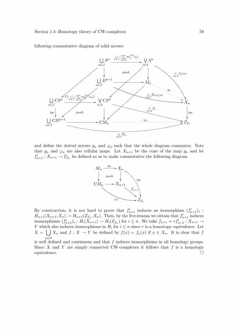
Section 1.4: Homotopy theory of CW-complexes 59
following commutative diagram of solid arrows
⊔α∈J
Snt
α∈J(
Pλ∈Λ
m(α)λ iλ)
//
push
||yyyyyyyyyyyyyyyyyyyyyyyy
∨i∈Λ
Sn
+
λ∈Λfλ|Sn
~~||||
||||
||||
||||
||||
|||
⊔α∈J
Dn+1
||yyyy
yyyy
yyyy
yyyy
yyyy
yyyy
tα∈J
Hα|CSn
//
//Mn
gn
''
~~||||
||||
||||
||||
||||
||||
||
⊔α∈J
CSnC( t
α∈J(
Pλ∈Λ
m(α)λ iλ))
//
inc
push
∨i∈Λ
CSn
+λ∈Λ
fλ
++WWWWWWWWWWWWWWWWWWWWWWWWWWWWWWWWWWWWW
Xn
inc
⊔α∈J
CDn+1 //
tα∈J
Hα
33CMnϕn // Zfn
and define the dotted arrows gn and ϕn such that the whole diagram commutes. Notethat gn and ϕn are also cellular maps. Let Xn+1 be the cone of the map gn and letf ′n+1 : Xn+1 → Zfn be defined so as to make commutative the following diagram
Mngn //
push
Xn
inc
CMn//
ϕn //
Xn+1f ′n+1
""FFFFFFFF
Zfn
By construction, it is not hard to prove that f ′n+1 induces an isomorphism (f ′n+1)∗ :Hn+1(Xn+1, Xn) → Hn+1(Zfn , Xn). Then, by the five-lemma we obtain that f ′n+1 inducesisomorphisms (f ′n+1)∗ : Hi(Xn+1) → Hi(Zfn) for i ≤ n. We take fn+1 = rf ′n+1 : Xn+1 →Y which also induces isomorphisms in Hi for i ≤ n since r is a homotopy equivalence. LetX =
⋃n∈N
Xn and f : X → Y be defined by f(x) = fn(x) if x ∈ Xn. It is clear that f
is well defined and continuous and that f induces isomorphisms in all homology groups.Since X and Y are simply connected CW-complexes it follows that f is a homotopyequivalence.
Chapter 2
Fibrations and spectral sequences
Spectral sequences constitute a powerful computational tool whose areas of applicationinclude algebra, topology and geometry. They where introduced by Leray in 1946 tocompute sheaf cohomology, but some years later other mathematicians noticed that hisidea could be applied to other settings. One of them was J.-P. Serre, who introduces aspectral sequence associated to fibration of topological spaces [17]. Serre spectral sequenceis a key tool in algebraic topology which has many applications including, for example,computations regarding homotopy groups of spheres and a generalization of Hurewicztheorem.
In the mid fifties, Federer also applies the machinery of spectral sequences to studyhomotopy groups of spaces of maps and develops the spectral sequence named after him.
In this chapter we begin by recalling the definition of fibrations and some basic prop-erties, such as the long exact homotopy sequence associated to a fibration. Then, we givethe definition and construction of Postnikov towers, which can be thought as a kind ofhomotopy decomposition.
In the third section we give an algebraic approach to spectral sequences with someexamples and results. We then introduce Serre spectral sequence in section 4, using in itsproof the algebraic results given before. We also include important applications of it, suchas the generalized version of Hurewicz theorem and some others about homotopy groupof spheres.
Section 5 deals with localization of topological spaces. The key theorem of this sectionis proved with the aid of Serre spectral sequence.
In the last section we give an alternative construction of Federer’s spectral sequence [6]which is useful to obtain information about A-homotopy groups of spaces. We also use itto prove a generalization of Hopf-Whitney theorem (2.5.6).
2.1 Fibrations
Fibrations constitute a class of continuous maps of great importance in algebraic topology.Together with cofibrations and weak equivalences they form the basis of classical homotopytheory and serve as models for abstract homotopy theories.
Before starting to work with fibrations we will define lifting properties so as to have
60
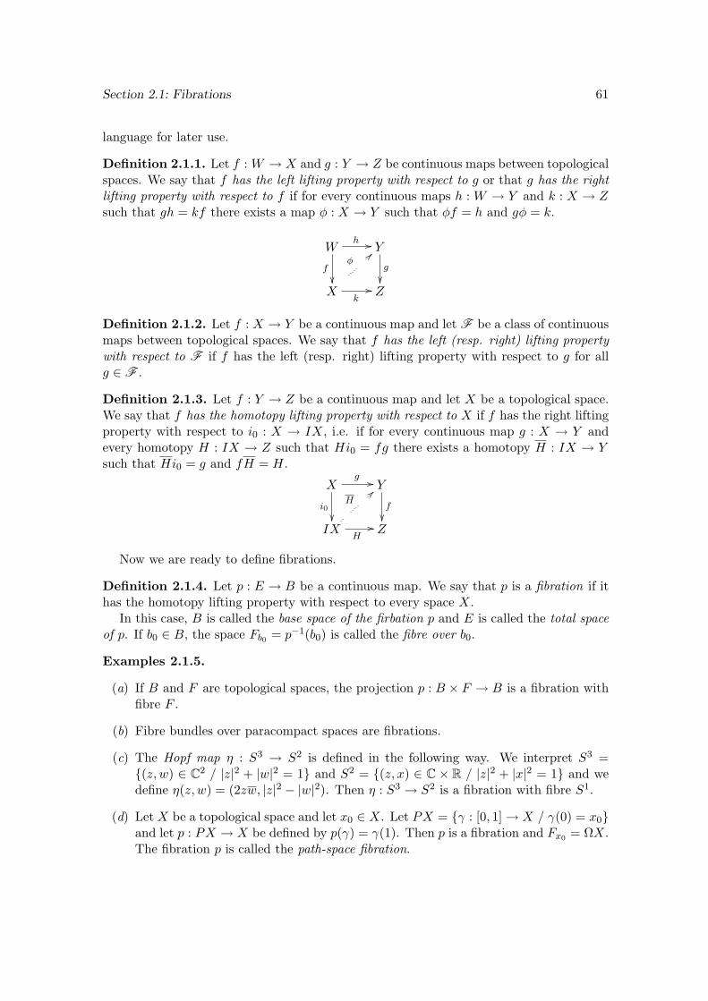
Section 2.1: Fibrations 61
language for later use.
Definition 2.1.1. Let f : W → X and g : Y → Z be continuous maps between topologicalspaces. We say that f has the left lifting property with respect to g or that g has the rightlifting property with respect to f if for every continuous maps h : W → Y and k : X → Zsuch that gh = kf there exists a map φ : X → Y such that φf = h and gφ = k.
Wh //
f
Y
g
X
k//
φ>>
Z
Definition 2.1.2. Let f : X → Y be a continuous map and let F be a class of continuousmaps between topological spaces. We say that f has the left (resp. right) lifting propertywith respect to F if f has the left (resp. right) lifting property with respect to g for allg ∈ F .
Definition 2.1.3. Let f : Y → Z be a continuous map and let X be a topological space.We say that f has the homotopy lifting property with respect to X if f has the right liftingproperty with respect to i0 : X → IX, i.e. if for every continuous map g : X → Y andevery homotopy H : IX → Z such that Hi0 = fg there exists a homotopy H : IX → Ysuch that Hi0 = g and fH = H.
Xg //
i0
Y
f
IXH//
H==
Z
Now we are ready to define fibrations.
Definition 2.1.4. Let p : E → B be a continuous map. We say that p is a fibration if ithas the homotopy lifting property with respect to every space X.
In this case, B is called the base space of the firbation p and E is called the total spaceof p. If b0 ∈ B, the space Fb0 = p−1(b0) is called the fibre over b0.
Examples 2.1.5.
(a) If B and F are topological spaces, the projection p : B × F → B is a fibration withfibre F .
(b) Fibre bundles over paracompact spaces are fibrations.
(c) The Hopf map η : S3 → S2 is defined in the following way. We interpret S3 =(z, w) ∈ C2 / |z|2 + |w|2 = 1 and S2 = (z, x) ∈ C × R / |z|2 + |x|2 = 1 and wedefine η(z, w) = (2zw, |z|2 − |w|2). Then η : S3 → S2 is a fibration with fibre S1.
(d) Let X be a topological space and let x0 ∈ X. Let PX = γ : [0, 1] → X / γ(0) = x0and let p : PX → X be defined by p(γ) = γ(1). Then p is a fibration and Fx0 = ΩX.The fibration p is called the path-space fibration.
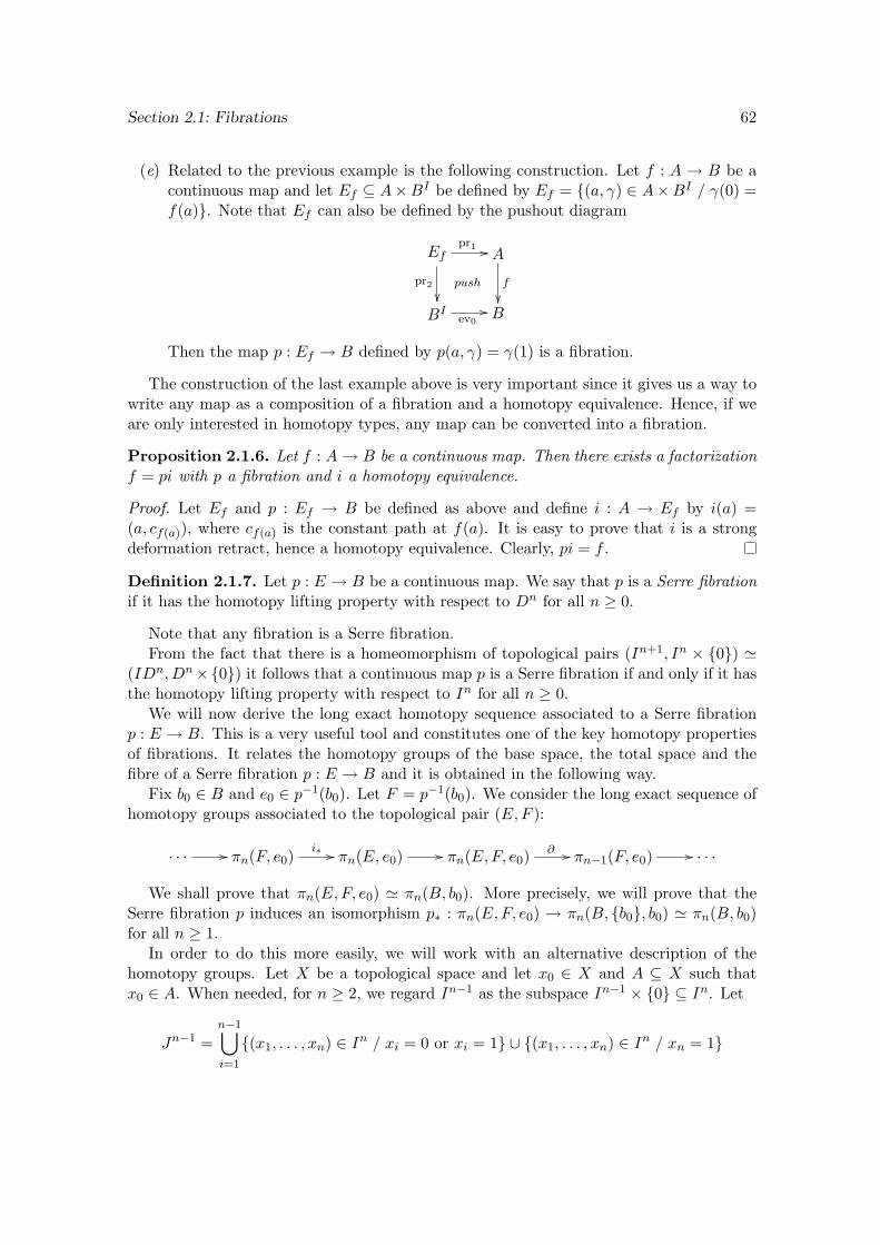
Section 2.1: Fibrations 62
(e) Related to the previous example is the following construction. Let f : A → B be acontinuous map and let Ef ⊆ A×BI be defined by Ef = (a, γ) ∈ A×BI / γ(0) =f(a). Note that Ef can also be defined by the pushout diagram
Efpr1 //
pr2
push
A
f
BI
ev0
// B
Then the map p : Ef → B defined by p(a, γ) = γ(1) is a fibration.
The construction of the last example above is very important since it gives us a way towrite any map as a composition of a fibration and a homotopy equivalence. Hence, if weare only interested in homotopy types, any map can be converted into a fibration.
Proposition 2.1.6. Let f : A→ B be a continuous map. Then there exists a factorizationf = pi with p a fibration and i a homotopy equivalence.
Proof. Let Ef and p : Ef → B be defined as above and define i : A → Ef by i(a) =(a, cf(a)), where cf(a) is the constant path at f(a). It is easy to prove that i is a strongdeformation retract, hence a homotopy equivalence. Clearly, pi = f .
Definition 2.1.7. Let p : E → B be a continuous map. We say that p is a Serre fibrationif it has the homotopy lifting property with respect to Dn for all n ≥ 0.
Note that any fibration is a Serre fibration.From the fact that there is a homeomorphism of topological pairs (In+1, In × 0) '
(IDn, Dn×0) it follows that a continuous map p is a Serre fibration if and only if it hasthe homotopy lifting property with respect to In for all n ≥ 0.
We will now derive the long exact homotopy sequence associated to a Serre fibrationp : E → B. This is a very useful tool and constitutes one of the key homotopy propertiesof fibrations. It relates the homotopy groups of the base space, the total space and thefibre of a Serre fibration p : E → B and it is obtained in the following way.
Fix b0 ∈ B and e0 ∈ p−1(b0). Let F = p−1(b0). We consider the long exact sequence ofhomotopy groups associated to the topological pair (E,F ):
. . . // πn(F, e0)i∗ // πn(E, e0) // πn(E,F, e0)
∂ // πn−1(F, e0) // . . .
We shall prove that πn(E,F, e0) ' πn(B, b0). More precisely, we will prove that theSerre fibration p induces an isomorphism p∗ : πn(E,F, e0) → πn(B, b0, b0) ' πn(B, b0)for all n ≥ 1.
In order to do this more easily, we will work with an alternative description of thehomotopy groups. Let X be a topological space and let x0 ∈ X and A ⊆ X such thatx0 ∈ A. When needed, for n ≥ 2, we regard In−1 as the subspace In−1 × 0 ⊆ In. Let
Jn−1 =n−1⋃i=1
(x1, . . . , xn) ∈ In / xi = 0 or xi = 1 ∪ (x1, . . . , xn) ∈ In / xn = 1
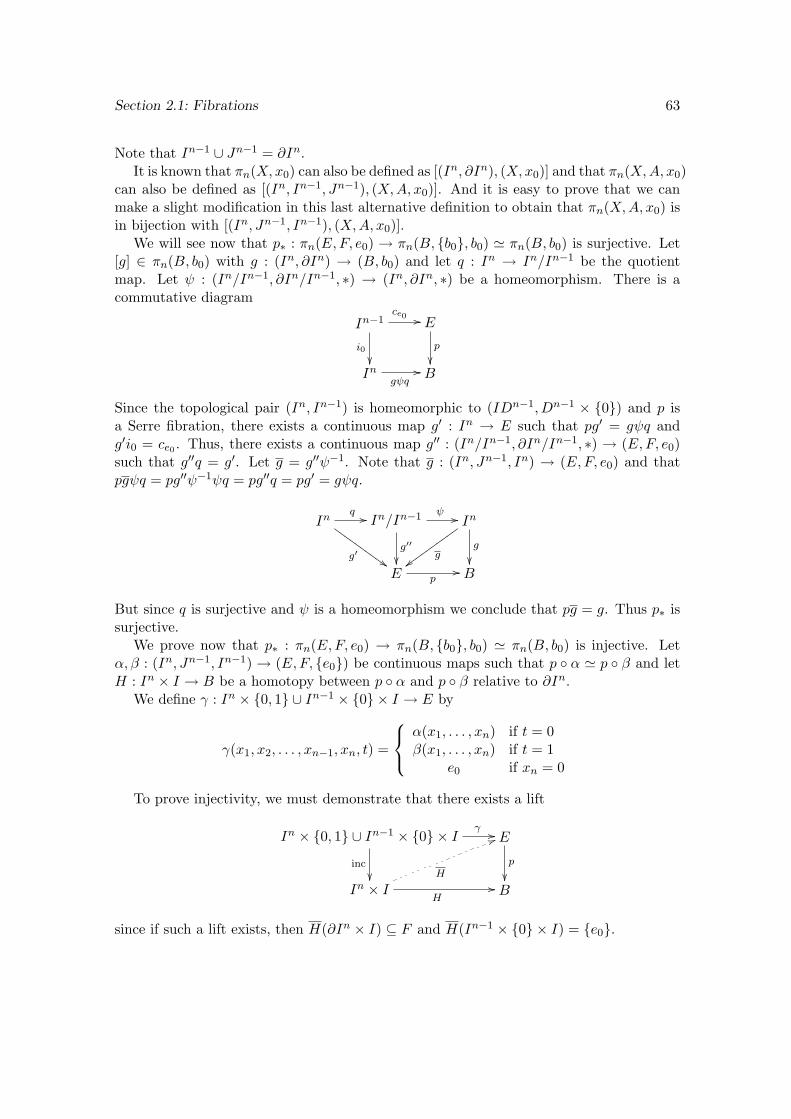
Section 2.1: Fibrations 63
Note that In−1 ∪ Jn−1 = ∂In.It is known that πn(X,x0) can also be defined as [(In, ∂In), (X,x0)] and that πn(X,A, x0)
can also be defined as [(In, In−1, Jn−1), (X,A, x0)]. And it is easy to prove that we canmake a slight modification in this last alternative definition to obtain that πn(X,A, x0) isin bijection with [(In, Jn−1, In−1), (X,A, x0)].
We will see now that p∗ : πn(E,F, e0) → πn(B, b0, b0) ' πn(B, b0) is surjective. Let[g] ∈ πn(B, b0) with g : (In, ∂In) → (B, b0) and let q : In → In/In−1 be the quotientmap. Let ψ : (In/In−1, ∂In/In−1, ∗) → (In, ∂In, ∗) be a homeomorphism. There is acommutative diagram
In−1ce0 //
i0
E
p
In
gψq// B
Since the topological pair (In, In−1) is homeomorphic to (IDn−1, Dn−1 × 0) and p isa Serre fibration, there exists a continuous map g′ : In → E such that pg′ = gψq andg′i0 = ce0 . Thus, there exists a continuous map g′′ : (In/In−1, ∂In/In−1, ∗) → (E,F, e0)such that g′′q = g′. Let g = g′′ψ−1. Note that g : (In, Jn−1, In) → (E,F, e0) and thatpgψq = pg′′ψ−1ψq = pg′′q = pg′ = gψq.
Inq //
g′ $$HHHHHHHHHH In/In−1 ψ //
g′′
In
g
gvvvvvvvvvv
E p// B
But since q is surjective and ψ is a homeomorphism we conclude that pg = g. Thus p∗ issurjective.
We prove now that p∗ : πn(E,F, e0) → πn(B, b0, b0) ' πn(B, b0) is injective. Letα, β : (In, Jn−1, In−1) → (E,F, e0) be continuous maps such that p α ' p β and letH : In × I → B be a homotopy between p α and p β relative to ∂In.
We define γ : In × 0, 1 ∪ In−1 × 0 × I → E by
γ(x1, x2, . . . , xn−1, xn, t) =
α(x1, . . . , xn) if t = 0β(x1, . . . , xn) if t = 1
e0 if xn = 0
To prove injectivity, we must demonstrate that there exists a lift
In × 0, 1 ∪ In−1 × 0 × Iγ //
inc
E
p
In × I
H//
H
55
B
since if such a lift exists, then H(∂In × I) ⊆ F and H(In−1 × 0 × I) = e0.
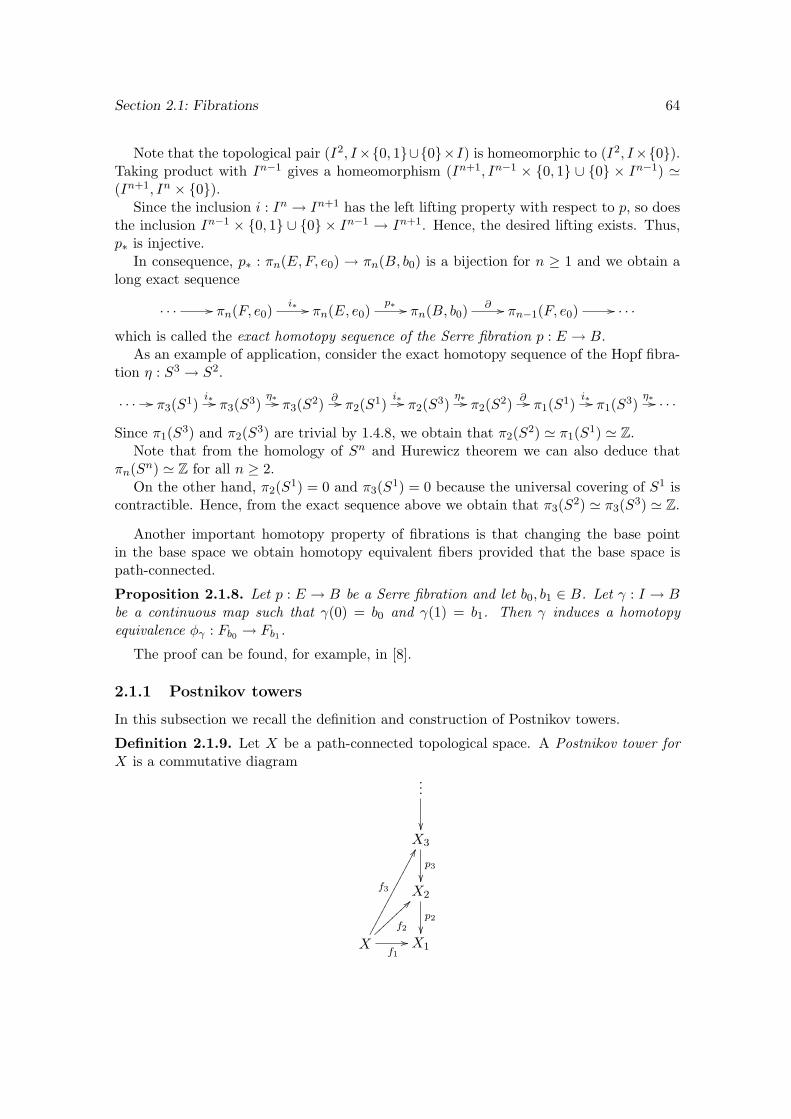
Section 2.1: Fibrations 64
Note that the topological pair (I2, I×0, 1∪0×I) is homeomorphic to (I2, I×0).Taking product with In−1 gives a homeomorphism (In+1, In−1 × 0, 1 ∪ 0 × In−1) '(In+1, In × 0).
Since the inclusion i : In → In+1 has the left lifting property with respect to p, so doesthe inclusion In−1 × 0, 1 ∪ 0 × In−1 → In+1. Hence, the desired lifting exists. Thus,p∗ is injective.
In consequence, p∗ : πn(E,F, e0) → πn(B, b0) is a bijection for n ≥ 1 and we obtain along exact sequence
. . . // πn(F, e0)i∗ // πn(E, e0)
p∗ // πn(B, b0)∂ // πn−1(F, e0) // . . .
which is called the exact homotopy sequence of the Serre fibration p : E → B.As an example of application, consider the exact homotopy sequence of the Hopf fibra-
tion η : S3 → S2.
. . . // π3(S1)i∗ // π3(S3)
η∗ // π3(S2) ∂ // π2(S1)i∗ // π2(S3)
η∗ // π2(S2) ∂ // π1(S1)i∗ // π1(S3)
η∗ // . . .
Since π1(S3) and π2(S3) are trivial by 1.4.8, we obtain that π2(S2) ' π1(S1) ' Z.Note that from the homology of Sn and Hurewicz theorem we can also deduce that
πn(Sn) ' Z for all n ≥ 2.On the other hand, π2(S1) = 0 and π3(S1) = 0 because the universal covering of S1 is
contractible. Hence, from the exact sequence above we obtain that π3(S2) ' π3(S3) ' Z.
Another important homotopy property of fibrations is that changing the base pointin the base space we obtain homotopy equivalent fibers provided that the base space ispath-connected.
Proposition 2.1.8. Let p : E → B be a Serre fibration and let b0, b1 ∈ B. Let γ : I → Bbe a continuous map such that γ(0) = b0 and γ(1) = b1. Then γ induces a homotopyequivalence φγ : Fb0 → Fb1.
The proof can be found, for example, in [8].
2.1.1 Postnikov towers
In this subsection we recall the definition and construction of Postnikov towers.
Definition 2.1.9. Let X be a path-connected topological space. A Postnikov tower forX is a commutative diagram
...
X3
p3X2
p2
Xf1//
f2
>>
f3
FFX1
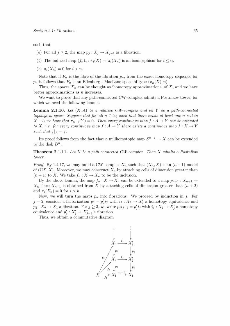
Section 2.1: Fibrations 65
such that
(a) For all j ≥ 2, the map pj : Xj → Xj−1 is a fibration.
(b) The induced map (fn)∗ : πi(X) → πi(Xn) is an isomorphism for i ≤ n.
(c) πi(Xn) = 0 for i > n.
Note that if Fn is the fibre of the fibration pn, from the exact homotopy sequence forpn it follows that Fn is an Eilenberg - MacLane space of type (πn(X), n).
Thus, the spaces Xn can be thought as ‘homotopy approximations’ of X, and we havebetter approximations as n increases.
We want to prove that any path-connected CW-complex admits a Postnikov tower, forwhich we need the following lemma.
Lemma 2.1.10. Let (X,A) be a relative CW-complex and let Y be a path-connectedtopological space. Suppose that for all n ∈ N0 such that there exists at least one n-cell inX−A we have that πn−1(Y ) = 0. Then every continuous map f : A→ Y can be extendedto X, i.e. for every continuous map f : A→ Y there exists a continuous map f : X → Ysuch that f |A = f .
Its proof follows from the fact that a nullhomotopic map Sn−1 → X can be extendedto the disk Dn.
Theorem 2.1.11. Let X be a path-connected CW-complex. Then X admits a Postnikovtower.
Proof. By 1.4.17, we may build a CW-complex Xn such that (Xn, X) is an (n+ 1)-modelof (CX,X). Moreover, we may construct Xn by attaching cells of dimension greater than(n+ 1) to X. We take fn : X → Xn to be the inclusion.
By the above lemma, the map fn : X → Xn can be extended to a map pn+1 : Xn+1 →Xn since Xn+1 is obtained from X by attaching cells of dimension greater than (n + 2)and πi(Xn) = 0 for i > n.
Now, we will turn the maps pn into fibrations. We proceed by induction in j. Forj = 2, consider a factorization p2 = p′2i2 with i2 : X2 → X ′2 a homotopy equivalence andp2 : X ′2 → X1 a fibration. For j ≥ 3, we write pjij−1 = p′jij with ij : Xj → X ′j a homotopyequivalence and p′j : X ′j → X ′j−1 a fibration.
Thus, we obtain a commutative diagram
...
...
X3
p3
i3 // X ′3
p′3
X2
p2
i2 // X ′2
p′2
Xf1//
f2
>>~~~~~~~~
f3
GGX1
i1=Id // X1
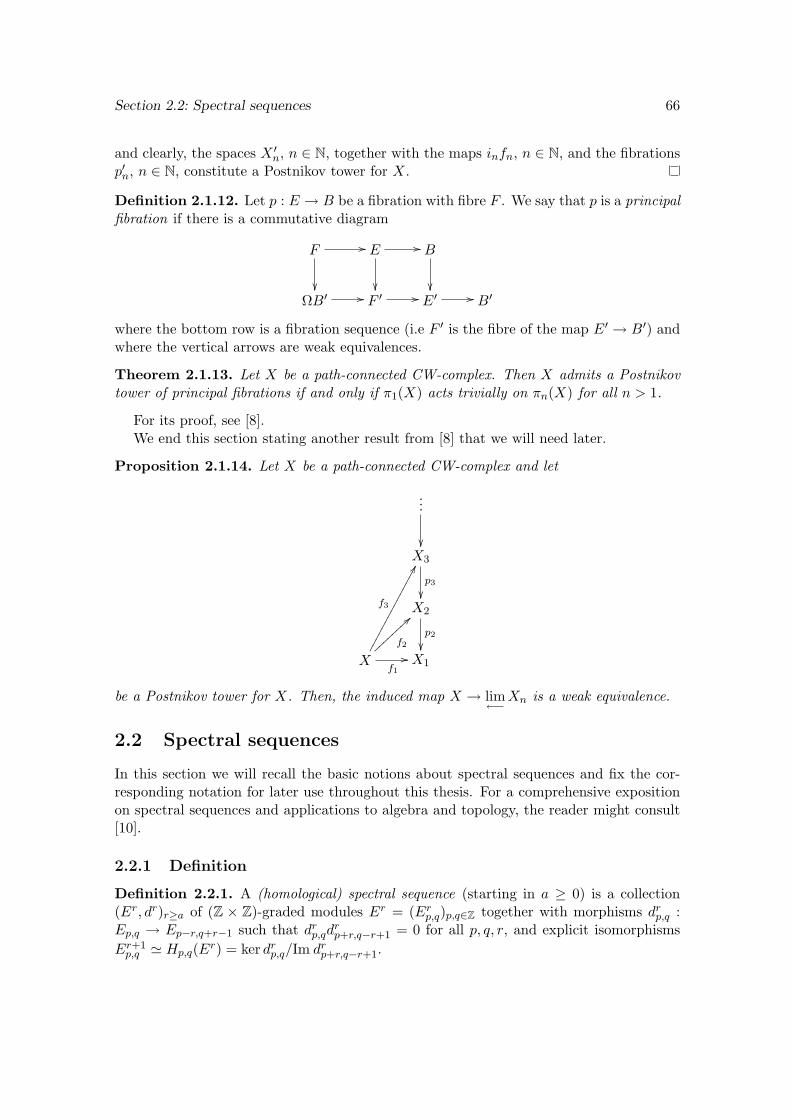
Section 2.2: Spectral sequences 66
and clearly, the spaces X ′n, n ∈ N, together with the maps infn, n ∈ N, and the fibrationsp′n, n ∈ N, constitute a Postnikov tower for X.
Definition 2.1.12. Let p : E → B be a fibration with fibre F . We say that p is a principalfibration if there is a commutative diagram
F //
E //
B
ΩB′ // F ′ // E′ // B′
where the bottom row is a fibration sequence (i.e F ′ is the fibre of the map E′ → B′) andwhere the vertical arrows are weak equivalences.
Theorem 2.1.13. Let X be a path-connected CW-complex. Then X admits a Postnikovtower of principal fibrations if and only if π1(X) acts trivially on πn(X) for all n > 1.
For its proof, see [8].We end this section stating another result from [8] that we will need later.
Proposition 2.1.14. Let X be a path-connected CW-complex and let
...
X3
p3X2
p2
Xf1//
f2
>>
f3
FFX1
be a Postnikov tower for X. Then, the induced map X → lim←−
Xn is a weak equivalence.
2.2 Spectral sequences
In this section we will recall the basic notions about spectral sequences and fix the cor-responding notation for later use throughout this thesis. For a comprehensive expositionon spectral sequences and applications to algebra and topology, the reader might consult[10].
2.2.1 Definition
Definition 2.2.1. A (homological) spectral sequence (starting in a ≥ 0) is a collection(Er, dr)r≥a of (Z × Z)-graded modules Er = (Erp,q)p,q∈Z together with morphisms drp,q :Ep,q → Ep−r,q+r−1 such that drp,qd
rp+r,q−r+1 = 0 for all p, q, r, and explicit isomorphisms
Er+1p,q ' Hp,q(Er) = ker drp,q/Im drp+r,q−r+1.
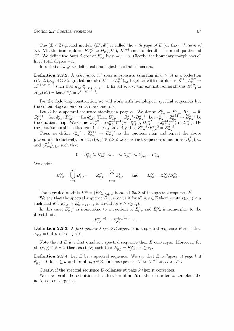
Section 2.2: Spectral sequences 67
The (Z × Z)-graded module (Er, dr) is called the r-th page of E (or the r-th term ofE). Via the isomorphism Er+1
p,q ' Hp,q(Er), Er+1 can be identified to a subquotient ofEr. We define the total degree of Erp,q by n = p+ q. Clearly, the boundary morphisms dr
have total degree −1.In a similar way we define cohomological spectral sequences.
Definition 2.2.2. A cohomological spectral sequence (starting in a ≥ 0) is a collection(Er, dr)r≥a of Z×Z-graded modules Er = (Ep,qr )p,q together with morphisms dp,qr : Ep,qr →Ep+r,q−r+1r such that drp,qd
rp−r,q+r−1 = 0 for all p, q, r, and explicit isomorphisms Ep,qr+1 '
Hp,q(Er) = ker dp,qr /Im dp−r,q+r−1r .
For the following construction we will work with homological spectral sequences butthe cohomological version can be done too.
Let E be a spectral sequence starting in page a. We define Zap,q = Eap,q, Bap,q = 0,
Za+1p,q = ker dap,q, B
a+1p,q = Im dap,q. Then Ea+1
p,q = Za+1p,q /B
a+1p,q . Let πa+1
p,q : Za+1p,q → Ea+1
p,q bethe quotient map. We define Za+2
p,q = (πa+1p,q )−1(ker da+1
p,q ), Ba+2p,q = (πa+1
p,q )−1(Im da+1p,q ). By
the first isomorphism theorem, it is easy to verify that Za+2p,q /B
a+2p,q = Ea+2
p,q .Thus, we define πa+2
p,q : Za+2p,q → Ea+2
p,q as the quotient map and repeat the aboveprocedure. Inductively, for each (p, q) ∈ Z×Z we construct sequences of modules (Bj
p,q)j≥aand (Zjp,q)j≥a such that
0 = Bap,q ⊆ Ba+1
p,q ⊆ . . . ⊆ Za+1p,q ⊆ Zap,q = Eap,q
We define
B∞p,q =∞⋃r=a
Brp,q , Z∞p,q =
∞⋂r=a
Zrp,q and E∞p,q = Z∞p,q/B∞p,q.
The bigraded module E∞ = (E∞p,q)p,q∈Z is called limit of the spectral sequence E.We say that the spectral sequence E converges if for all p, q ∈ Z there exists r(p, q) ≥ a
such that dr : Erp,q → Erp−r,q+r−1 is trivial for r ≥ r(p, q).In this case, Er+1
p,q is isomorphic to a quotient of Erp,q and E∞p,q is isomorphic to thedirect limit
Er(p,q)p,q → Er(p,q)+1p,q → . . .
Definition 2.2.3. A first quadrant spectral sequence is a spectral sequence E such thatEp,q = 0 if p < 0 or q < 0.
Note that if E is a first quadrant spectral sequence then E converges. Moreover, forall (p, q) ∈ Z× Z there exists r0 such that Erp,q = E∞p,q if r ≥ r0.
Definition 2.2.4. Let E be a spectral sequence. We say that E collapses at page k ifdrp,q = 0 for r ≥ k and for all p, q ∈ Z. In consequence, Er ' Er+1 ' . . . ' E∞.
Clearly, if the spectral sequence E collapses at page k then it converges.We now recall the definition of a filtration of an R-module in order to complete the
notion of convergence.
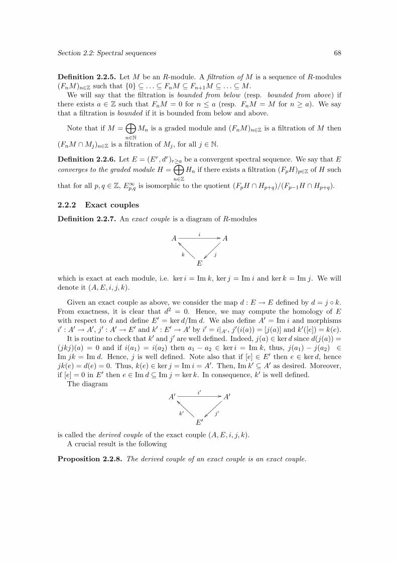
Section 2.2: Spectral sequences 68
Definition 2.2.5. Let M be an R-module. A filtration of M is a sequence of R-modules(FnM)n∈Z such that 0 ⊆ . . . ⊆ FnM ⊆ Fn+1M ⊆ . . . ⊆M .
We will say that the filtration is bounded from below (resp. bounded from above) ifthere exists a ∈ Z such that FnM = 0 for n ≤ a (resp. FnM = M for n ≥ a). We saythat a filtration is bounded if it is bounded from below and above.
Note that if M =⊕n∈N
Mn is a graded module and (FnM)n∈Z is a filtration of M then
(FnM ∩Mj)n∈Z is a filtration of Mj , for all j ∈ N.
Definition 2.2.6. Let E = (Er, dr)r≥a be a convergent spectral sequence. We say that Econverges to the graded module H =
⊕n∈Z
Hn if there exists a filtration (FpH)p∈Z of H such
that for all p, q ∈ Z, E∞p,q is isomorphic to the quotient (FpH ∩Hp+q)/(Fp−1H ∩Hp+q).
2.2.2 Exact couples
Definition 2.2.7. An exact couple is a diagram of R-modules
Ai // A
j~~~~
~~~
E
k
__@@@@@@@
which is exact at each module, i.e. ker i = Im k, ker j = Im i and ker k = Im j. We willdenote it (A,E, i, j, k).
Given an exact couple as above, we consider the map d : E → E defined by d = j k.From exactness, it is clear that d2 = 0. Hence, we may compute the homology of Ewith respect to d and define E′ = ker d/Im d. We also define A′ = Im i and morphismsi′ : A′ → A′, j′ : A′ → E′ and k′ : E′ → A′ by i′ = i|A′ , j′(i(a)) = [j(a)] and k′([e]) = k(e).
It is routine to check that k′ and j′ are well defined. Indeed, j(a) ∈ ker d since d(j(a)) =(jkj)(a) = 0 and if i(a1) = i(a2) then a1 − a2 ∈ ker i = Im k, thus, j(a1) − j(a2) ∈Im jk = Im d. Hence, j is well defined. Note also that if [e] ∈ E′ then e ∈ ker d, hencejk(e) = d(e) = 0. Thus, k(e) ∈ ker j = Im i = A′. Then, Im k′ ⊆ A′ as desired. Moreover,if [e] = 0 in E′ then e ∈ Im d ⊆ Im j = ker k. In consequence, k′ is well defined.
The diagram
A′i′ // A′
j′~~
E′k′
``AAAAAAAA
is called the derived couple of the exact couple (A,E, i, j, k).A crucial result is the following
Proposition 2.2.8. The derived couple of an exact couple is an exact couple.
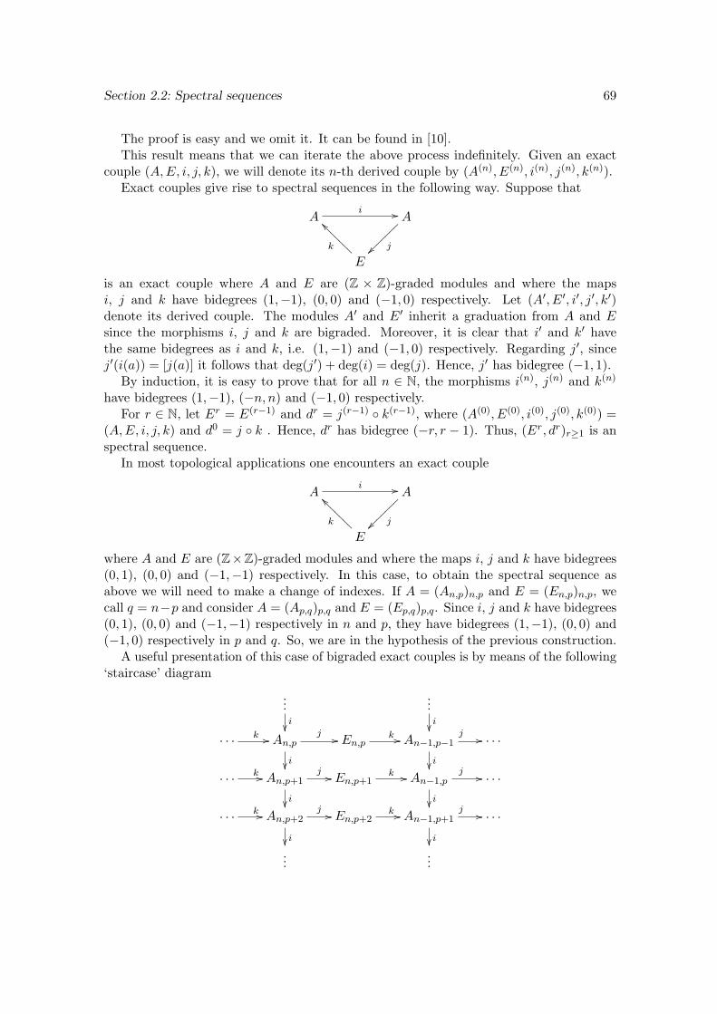
Section 2.2: Spectral sequences 69
The proof is easy and we omit it. It can be found in [10].This result means that we can iterate the above process indefinitely. Given an exact
couple (A,E, i, j, k), we will denote its n-th derived couple by (A(n), E(n), i(n), j(n), k(n)).Exact couples give rise to spectral sequences in the following way. Suppose that
Ai // A
j~~~~
~~~
E
k
__@@@@@@@
is an exact couple where A and E are (Z × Z)-graded modules and where the mapsi, j and k have bidegrees (1,−1), (0, 0) and (−1, 0) respectively. Let (A′, E′, i′, j′, k′)denote its derived couple. The modules A′ and E′ inherit a graduation from A and Esince the morphisms i, j and k are bigraded. Moreover, it is clear that i′ and k′ havethe same bidegrees as i and k, i.e. (1,−1) and (−1, 0) respectively. Regarding j′, sincej′(i(a)) = [j(a)] it follows that deg(j′) + deg(i) = deg(j). Hence, j′ has bidegree (−1, 1).
By induction, it is easy to prove that for all n ∈ N, the morphisms i(n), j(n) and k(n)
have bidegrees (1,−1), (−n, n) and (−1, 0) respectively.For r ∈ N, let Er = E(r−1) and dr = j(r−1) k(r−1), where (A(0), E(0), i(0), j(0), k(0)) =
(A,E, i, j, k) and d0 = j k . Hence, dr has bidegree (−r, r − 1). Thus, (Er, dr)r≥1 is anspectral sequence.
In most topological applications one encounters an exact couple
Ai // A
j~~~~
~~~
E
k
__@@@@@@@
where A and E are (Z×Z)-graded modules and where the maps i, j and k have bidegrees(0, 1), (0, 0) and (−1,−1) respectively. In this case, to obtain the spectral sequence asabove we will need to make a change of indexes. If A = (An,p)n,p and E = (En,p)n,p, wecall q = n−p and consider A = (Ap,q)p,q and E = (Ep,q)p,q. Since i, j and k have bidegrees(0, 1), (0, 0) and (−1,−1) respectively in n and p, they have bidegrees (1,−1), (0, 0) and(−1, 0) respectively in p and q. So, we are in the hypothesis of the previous construction.
A useful presentation of this case of bigraded exact couples is by means of the following‘staircase’ diagram
...i
...i
. . . k // An,pj //
i
En,pk // An−1,p−1
j //
i
. . .
. . . k // An,p+1j //
i
En,p+1k // An−1,p
j //
i
. . .
. . . k // An,p+2j //
i
En,p+2k // An−1,p+1
j //
i
. . .
......
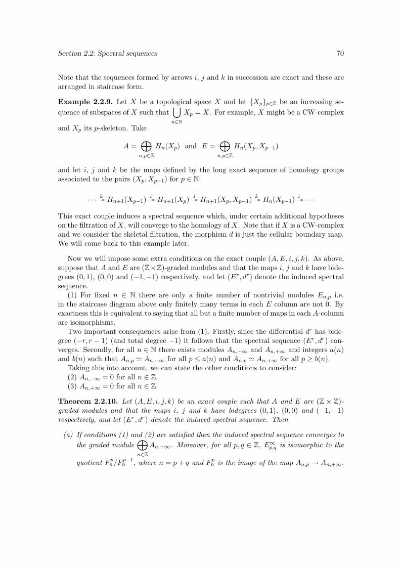
Section 2.2: Spectral sequences 70
Note that the sequences formed by arrows i, j and k in succession are exact and these arearranged in staircase form.
Example 2.2.9. Let X be a topological space X and let Xpp∈Z be an increasing se-quence of subspaces of X such that
⋃n∈N
Xp = X. For example, X might be a CW-complex
and Xp its p-skeleton. Take
A =⊕n,p∈Z
Hn(Xp) and E =⊕n,p∈Z
Hn(Xp, Xp−1)
and let i, j and k be the maps defined by the long exact sequence of homology groupsassociated to the pairs (Xp, Xp−1) for p ∈ N:
. . . k // Hn+1(Xp−1)i // Hn+1(Xp)
j // Hn+1(Xp, Xp−1)k // Hn(Xp−1)
i // . . .
This exact couple induces a spectral sequence which, under certain additional hypotheseson the filtration of X, will converge to the homology of X. Note that if X is a CW-complexand we consider the skeletal filtration, the morphism d is just the cellular boundary map.We will come back to this example later.
Now we will impose some extra conditions on the exact couple (A,E, i, j, k). As above,suppose that A and E are (Z×Z)-graded modules and that the maps i, j and k have bide-grees (0, 1), (0, 0) and (−1,−1) respectively, and let (Er, dr) denote the induced spectralsequence.
(1) For fixed n ∈ N there are only a finite number of nontrivial modules En,p i.e.in the staircase diagram above only finitely many terms in each E column are not 0. Byexactness this is equivalent to saying that all but a finite number of maps in each A-columnare isomorphisms.
Two important consequences arise from (1). Firstly, since the differential dr has bide-gree (−r, r − 1) (and total degree −1) it follows that the spectral sequence (Er, dr) con-verges. Secondly, for all n ∈ N there exists modules An,−∞ and An,+∞ and integers a(n)and b(n) such that An,p ' An,−∞ for all p ≤ a(n) and An,p ' An,+∞ for all p ≥ b(n).
Taking this into account, we can state the other conditions to consider:(2) An,−∞ = 0 for all n ∈ Z.(3) An,+∞ = 0 for all n ∈ Z.
Theorem 2.2.10. Let (A,E, i, j, k) be an exact couple such that A and E are (Z × Z)-graded modules and that the maps i, j and k have bidegrees (0, 1), (0, 0) and (−1,−1)respectively, and let (Er, dr) denote the induced spectral sequence. Then
(a) If conditions (1) and (2) are satisfied then the induced spectral sequence converges tothe graded module
⊕n∈Z
An,+∞. Moreover, for all p, q ∈ Z, E∞p,q is isomorphic to the
quotient F pn/Fp−1n , where n = p+ q and F pn is the image of the map An,p → An,+∞.
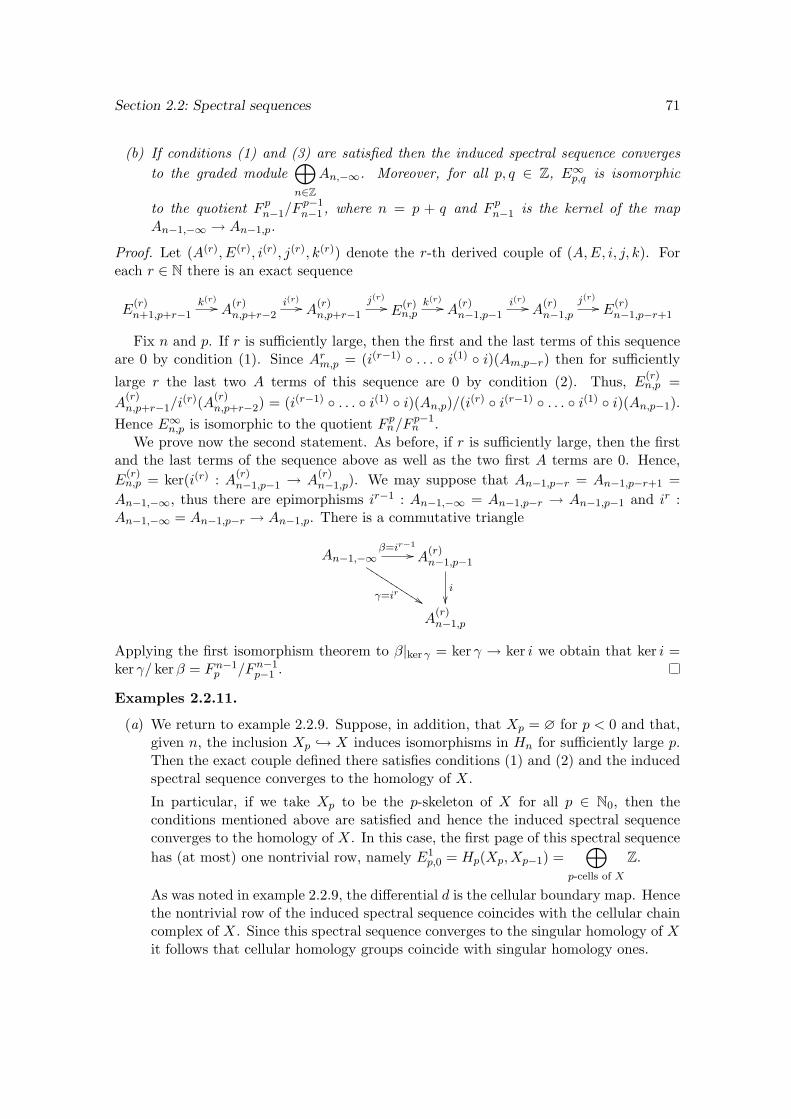
Section 2.2: Spectral sequences 71
(b) If conditions (1) and (3) are satisfied then the induced spectral sequence convergesto the graded module
⊕n∈Z
An,−∞. Moreover, for all p, q ∈ Z, E∞p,q is isomorphic
to the quotient F pn−1/Fp−1n−1 , where n = p + q and F pn−1 is the kernel of the map
An−1,−∞ → An−1,p.
Proof. Let (A(r), E(r), i(r), j(r), k(r)) denote the r-th derived couple of (A,E, i, j, k). Foreach r ∈ N there is an exact sequence
E(r)n+1,p+r−1
k(r)// A
(r)n,p+r−2
i(r)// A
(r)n,p+r−1
j(r)// E
(r)n,p
k(r)// A
(r)n−1,p−1
i(r)// A
(r)n−1,p
j(r)// E
(r)n−1,p−r+1
Fix n and p. If r is sufficiently large, then the first and the last terms of this sequenceare 0 by condition (1). Since Arm,p = (i(r−1) . . . i(1) i)(Am,p−r) then for sufficiently
large r the last two A terms of this sequence are 0 by condition (2). Thus, E(r)n,p =
A(r)n,p+r−1/i
(r)(A(r)n,p+r−2) = (i(r−1) . . . i(1) i)(An,p)/(i(r) i(r−1) . . . i(1) i)(An,p−1).
Hence E∞n,p is isomorphic to the quotient F pn/Fp−1n .
We prove now the second statement. As before, if r is sufficiently large, then the firstand the last terms of the sequence above as well as the two first A terms are 0. Hence,E
(r)n,p = ker(i(r) : A(r)
n−1,p−1 → A(r)n−1,p). We may suppose that An−1,p−r = An−1,p−r+1 =
An−1,−∞, thus there are epimorphisms ir−1 : An−1,−∞ = An−1,p−r → An−1,p−1 and ir :An−1,−∞ = An−1,p−r → An−1,p. There is a commutative triangle
An−1,−∞β=ir−1
//
γ=ir %%JJJJJJJJJJJ A(r)n−1,p−1
i
A(r)n−1,p
Applying the first isomorphism theorem to β|ker γ = ker γ → ker i we obtain that ker i =ker γ/ kerβ = Fn−1
p /Fn−1p−1 .
Examples 2.2.11.
(a) We return to example 2.2.9. Suppose, in addition, that Xp = ∅ for p < 0 and that,given n, the inclusion Xp → X induces isomorphisms in Hn for sufficiently large p.Then the exact couple defined there satisfies conditions (1) and (2) and the inducedspectral sequence converges to the homology of X.
In particular, if we take Xp to be the p-skeleton of X for all p ∈ N0, then theconditions mentioned above are satisfied and hence the induced spectral sequenceconverges to the homology of X. In this case, the first page of this spectral sequencehas (at most) one nontrivial row, namely E1
p,0 = Hp(Xp, Xp−1) =⊕
p-cells of X
Z.
As was noted in example 2.2.9, the differential d is the cellular boundary map. Hencethe nontrivial row of the induced spectral sequence coincides with the cellular chaincomplex of X. Since this spectral sequence converges to the singular homology of Xit follows that cellular homology groups coincide with singular homology ones.
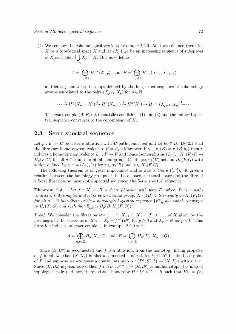
Section 2.3: Serre spectral sequence 72
(b) We see now the cohomological version of example 2.2.9. As it was defined there, letX be a topological space X and let Xpp∈Z be an increasing sequence of subspacesof X such that
⋃n∈N
Xp = X. But now define
A =⊕n,p∈Z
H−n(X−p) and E =⊕n,p∈Z
H−n(X−p, X−p−1)
and let i, j and k be the maps defined by the long exact sequence of cohomologygroups associated to the pairs (Xp+1, Xp) for p ∈ N:
. . . j // Hn(Xp+1, Xp)k // Hn(Xp+1)
i // Hn(Xp)j // Hn+1(Xp+1, Xp)
k // . . .
The exact couple (A,E, i, j, k) satisfies conditions (1) and (3) and the induced spec-tral sequence converges to the cohomology of X.
2.3 Serre spectral sequence
Let p : E → B be a Serre fibration with B path-connected and let b0 ∈ B. By 2.1.8 allthe fibres are homotopy equivalent to F = Fb0 . Moreover, if γ ∈ π1(B) = π1(B, b0) then γinduces a homotopy equivalence Lγ : F → F and hence isomorphisms (Lγ)∗ : Hn(F,G) →Hn(F,G) for all n ∈ N and for all abelian groups G. Hence, π1(B) acts on Hn(F,G) withaction defined by γ.x = (Lγ)∗(x) for γ ∈ π1(B) and x ∈ Hn(F,G).
The following theorem is of great importance and is due to Serre ([17]). It gives arelation between the homology groups of the base space, the total space and the fibre ofa Serre fibration by means of a spectral sequence: the Serre spectral sequence.
Theorem 2.3.1. Let f : X → B a Serre fibration with fibre F , where B is a path-connected CW-complex and let G be an abelian group. If π1(B) acts trivially on Hn(F ;G)for all n ∈ N then there exists a homological spectral sequence Erp,q, dr which convergesto H∗(X;G) and such that E2
p,q ' Hp(B;Hq(F ;G)).
Proof. We consider the filtration ∅ ⊆ . . . ⊆ X−1 ⊆ X0 ⊆ X1 ⊆ . . . of X given by thepreimages of the skeletons of B, i.e. Xp = f−1(Bp) for p ≥ 0 and Xp = ∅ for p < 0. Thisfiltration induces an exact couple as in example 2.2.9 with
A =⊕n,p∈Z
Hn(Xp;G) and E =⊕n,p∈Z
Hn(Xp, Xp−1;G).
Since (B,Bp) is p-connected and f is a fibration, from the homotopy lifting propertyof f it follows that (X,Xp) is also p-connected. Indeed, let b0 ∈ B0 be the base pointof B and suppose we are given a continuous map α : (Dr, Sr−1) → (X,Xp) with r ≤ n.Since (B,Bp) is p-connected then fα : (Dr, Sr−1) → (B,Bp) is nullhomotopic (as map oftopological pairs). Hence, there exists a homotopy H : Dr × I → B such that Hi0 = fα,
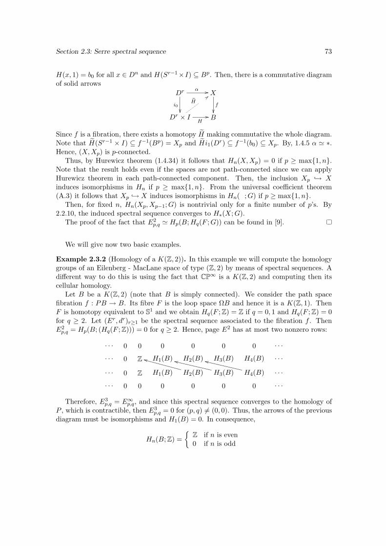
Section 2.3: Serre spectral sequence 73
H(x, 1) = b0 for all x ∈ Dn and H(Sr−1×I) ⊆ Bp. Then, there is a commutative diagramof solid arrows
Dr α //
i0
X
f
Dr × I
H//
eH ;;
B
Since f is a fibration, there exists a homotopy H making commutative the whole diagram.Note that H(Sr−1 × I) ⊆ f−1(Bp) = Xp and Hi1(Dr) ⊆ f−1(b0) ⊆ Xp. By, 1.4.5 α ' ∗.Hence, (X,Xp) is p-connected.
Thus, by Hurewicz theorem (1.4.34) it follows that Hn(X,Xp) = 0 if p ≥ max1, n.Note that the result holds even if the spaces are not path-connected since we can applyHurewicz theorem in each path-connected component. Then, the inclusion Xp → Xinduces isomorphisms in Hn if p ≥ max1, n. From the universal coefficient theorem(A.3) it follows that Xp → X induces isomorphisms in Hn( ;G) if p ≥ max1, n.
Then, for fixed n, Hn(Xp, Xp−1;G) is nontrivial only for a finite number of p’s. By2.2.10, the induced spectral sequence converges to H∗(X;G).
The proof of the fact that E2p,q ' Hp(B;Hq(F ;G)) can be found in [9].
We will give now two basic examples.
Example 2.3.2 (Homology of a K(Z, 2)). In this example we will compute the homologygroups of an Eilenberg - MacLane space of type (Z, 2) by means of spectral sequences. Adifferent way to do this is using the fact that CP∞ is a K(Z, 2) and computing then itscellular homology.
Let B be a K(Z, 2) (note that B is simply connected). We consider the path spacefibration f : PB → B. Its fibre F is the loop space ΩB and hence it is a K(Z, 1). ThenF is homotopy equivalent to S1 and we obtain Hq(F ; Z) = Z if q = 0, 1 and Hq(F ; Z) = 0for q ≥ 2. Let (Er, dr)r≥1 be the spectral sequence associated to the fibration f . ThenE2p,q = Hp(B; (Hq(F ; Z))) = 0 for q ≥ 2. Hence, page E2 has at most two nonzero rows:
. . . 0 0 0 0 0 0 . . .
. . . 0 Z H1(B) H2(B) H3(B) H4(B) . . .
. . . 0 Z H1(B) H2(B)
kkWWWWWWWWWWWWH3(B)
kkXXXXXXXXXXXXH4(B)
kkXXXXXXXXXXXX. . .
. . . 0 0 0 0 0 0 . . .
Therefore, E3p,q = E∞p,q, and since this spectral sequence converges to the homology of
P , which is contractible, then E3p,q = 0 for (p, q) 6= (0, 0). Thus, the arrows of the previous
diagram must be isomorphisms and H1(B) = 0. In consequence,
Hn(B; Z) =
Z if n is even0 if n is odd
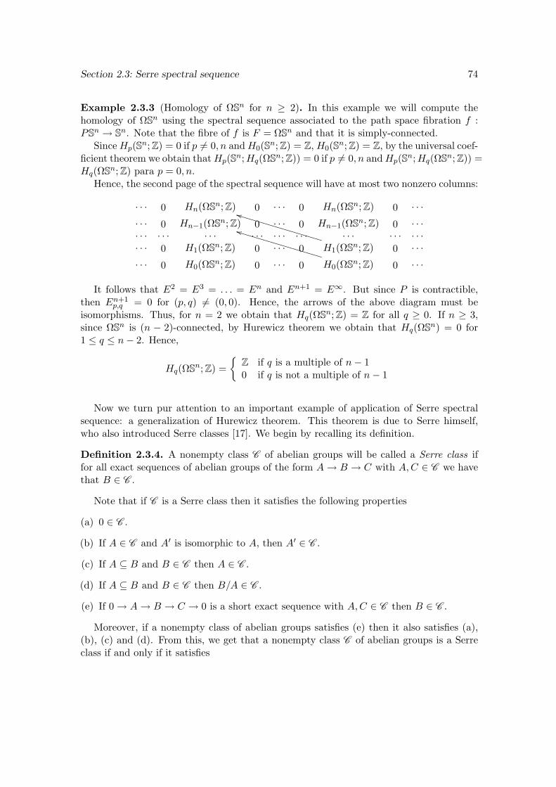
Section 2.3: Serre spectral sequence 74
Example 2.3.3 (Homology of ΩSn for n ≥ 2). In this example we will compute thehomology of ΩSn using the spectral sequence associated to the path space fibration f :PSn → Sn. Note that the fibre of f is F = ΩSn and that it is simply-connected.
SinceHp(Sn; Z) = 0 if p 6= 0, n andH0(Sn; Z) = Z, H0(Sn; Z) = Z, by the universal coef-ficient theorem we obtain thatHp(Sn;Hq(ΩSn; Z)) = 0 if p 6= 0, n andHp(Sn;Hq(ΩSn; Z)) =Hq(ΩSn; Z) para p = 0, n.
Hence, the second page of the spectral sequence will have at most two nonzero columns:
. . . 0 Hn(ΩSn; Z) 0 . . . 0 Hn(ΩSn; Z) 0 . . .
. . . 0 Hn−1(ΩSn; Z) 0 . . . 0 Hn−1(ΩSn; Z) 0 . . .
. . . . . . . . . . . . . . . . . . . . . . . . . . .
. . . 0 H1(ΩSn; Z) 0 . . . 0 H1(ΩSn; Z)
jjVVVVVVVVVVVVVVVVVVV
0 . . .
. . . 0 H0(ΩSn; Z) 0 . . . 0 H0(ΩSn; Z)
jjVVVVVVVVVVVVVVVVVVV
0 . . .
It follows that E2 = E3 = . . . = En and En+1 = E∞. But since P is contractible,then En+1
p,q = 0 for (p, q) 6= (0, 0). Hence, the arrows of the above diagram must beisomorphisms. Thus, for n = 2 we obtain that Hq(ΩSn; Z) = Z for all q ≥ 0. If n ≥ 3,since ΩSn is (n − 2)-connected, by Hurewicz theorem we obtain that Hq(ΩSn) = 0 for1 ≤ q ≤ n− 2. Hence,
Hq(ΩSn; Z) =
Z if q is a multiple of n− 10 if q is not a multiple of n− 1
Now we turn pur attention to an important example of application of Serre spectralsequence: a generalization of Hurewicz theorem. This theorem is due to Serre himself,who also introduced Serre classes [17]. We begin by recalling its definition.
Definition 2.3.4. A nonempty class C of abelian groups will be called a Serre class iffor all exact sequences of abelian groups of the form A→ B → C with A,C ∈ C we havethat B ∈ C .
Note that if C is a Serre class then it satisfies the following properties
(a) 0 ∈ C .
(b) If A ∈ C and A′ is isomorphic to A, then A′ ∈ C .
(c) If A ⊆ B and B ∈ C then A ∈ C .
(d) If A ⊆ B and B ∈ C then B/A ∈ C .
(e) If 0 → A→ B → C → 0 is a short exact sequence with A,C ∈ C then B ∈ C .
Moreover, if a nonempty class of abelian groups satisfies (e) then it also satisfies (a),(b), (c) and (d). From this, we get that a nonempty class C of abelian groups is a Serreclass if and only if it satisfies
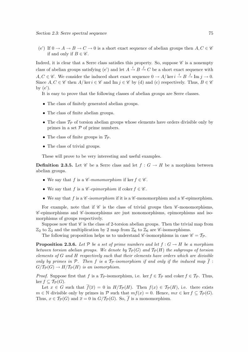
Section 2.3: Serre spectral sequence 75
(e’) If 0 → A→ B → C → 0 is a short exact sequence of abelian groups then A,C ∈ Cif and only if B ∈ C .
Indeed, it is clear that a Serre class satisfies this property. So, suppose C is a nonemptyclass of abelian groups satisfying (e’) and let A i→ B
j→ C be a short exact sequence with
A,C ∈ C . We consider the induced short exact sequence 0 → A/ ker i i→ Bj→ Im j → 0.
Since A,C ∈ C then A/ ker i ∈ C and Im j ∈ C by (d) and (c) respectively. Thus, B ∈ Cby (e’).
It is easy to prove that the following classes of abelian groups are Serre classes.
• The class of finitely generated abelian groups.
• The class of finite abelian groups.
• The class TP of torsion abelian groups whose elements have orders divisible only byprimes in a set P of prime numbers.
• The class of finite groups in TP .
• The class of trivial groups.
These will prove to be very interesting and useful examples.
Definition 2.3.5. Let C be a Serre class and let f : G → H be a morphism betweenabelian groups.
• We say that f is a C -monomorphism if ker f ∈ C .
• We say that f is a C -epimorphism if coker f ∈ C .
• We say that f is a C -isomorphism if it is a C -monomorphism and a C -epimorphism.
For example, note that if C is the class of trivial groups then C -monomorphisms,C -epimorphisms and C -isomorphisms are just monomorphisms, epimorphisms and iso-morphisms of groups respectively.
Suppose now that C is the class of 2-torsion abelian groups. Then the trivial map fromZ2 to Z2 and the multiplication by 2 map from Z6 to Z6 are C -isomorphisms.
The following proposition helps us to understand C -isomorphisms in case C = TP .
Proposition 2.3.6. Let P be a set of prime numbers and let f : G → H be a morphismbetween torsion abelian groups. We denote by TP(G) and TP(H) the subgroups of torsionelements of G and H respectively such that their elements have orders which are divisibleonly by primes in P. Then f is a TP-isomorphism if and only if the induced map f :G/TP(G) → H/TP(H) is an isomorphism.
Proof. Suppose first that f is a TP -isomorphism, i.e. ker f ∈ TP and coker f ∈ TP . Thus,ker f ⊆ TP(G).
Let x ∈ G such that f(x) = 0 in H/TP(H). Then f(x) ∈ TP(H), i.e. there existsm ∈ N divisible only by primes in P such that mf(x) = 0. Hence, mx ∈ ker f ⊆ TP(G).Thus, x ∈ TP(G) and x = 0 in G/TP(G). So, f is a monomorphism.
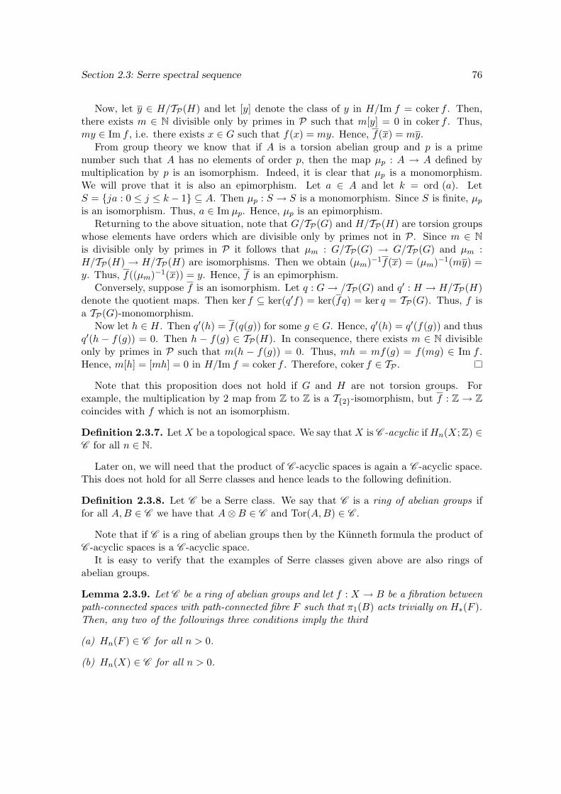
Section 2.3: Serre spectral sequence 76
Now, let y ∈ H/TP(H) and let [y] denote the class of y in H/Im f = coker f . Then,there exists m ∈ N divisible only by primes in P such that m[y] = 0 in coker f . Thus,my ∈ Im f , i.e. there exists x ∈ G such that f(x) = my. Hence, f(x) = my.
From group theory we know that if A is a torsion abelian group and p is a primenumber such that A has no elements of order p, then the map µp : A → A defined bymultiplication by p is an isomorphism. Indeed, it is clear that µp is a monomorphism.We will prove that it is also an epimorphism. Let a ∈ A and let k = ord (a). LetS = ja : 0 ≤ j ≤ k − 1 ⊆ A. Then µp : S → S is a monomorphism. Since S is finite, µpis an isomorphism. Thus, a ∈ Im µp. Hence, µp is an epimorphism.
Returning to the above situation, note that G/TP(G) and H/TP(H) are torsion groupswhose elements have orders which are divisible only by primes not in P. Since m ∈ Nis divisible only by primes in P it follows that µm : G/TP(G) → G/TP(G) and µm :H/TP(H) → H/TP(H) are isomorphisms. Then we obtain (µm)−1f(x) = (µm)−1(my) =y. Thus, f((µm)−1(x)) = y. Hence, f is an epimorphism.
Conversely, suppose f is an isomorphism. Let q : G→ /TP(G) and q′ : H → H/TP(H)denote the quotient maps. Then ker f ⊆ ker(q′f) = ker(fq) = ker q = TP(G). Thus, f isa TP(G)-monomorphism.
Now let h ∈ H. Then q′(h) = f(q(g)) for some g ∈ G. Hence, q′(h) = q′(f(g)) and thusq′(h − f(g)) = 0. Then h − f(g) ∈ TP(H). In consequence, there exists m ∈ N divisibleonly by primes in P such that m(h − f(g)) = 0. Thus, mh = mf(g) = f(mg) ∈ Im f .Hence, m[h] = [mh] = 0 in H/Im f = coker f . Therefore, coker f ∈ TP .
Note that this proposition does not hold if G and H are not torsion groups. Forexample, the multiplication by 2 map from Z to Z is a T2-isomorphism, but f : Z → Zcoincides with f which is not an isomorphism.
Definition 2.3.7. LetX be a topological space. We say thatX is C -acyclic ifHn(X; Z) ∈C for all n ∈ N.
Later on, we will need that the product of C -acyclic spaces is again a C -acyclic space.This does not hold for all Serre classes and hence leads to the following definition.
Definition 2.3.8. Let C be a Serre class. We say that C is a ring of abelian groups iffor all A,B ∈ C we have that A⊗B ∈ C and Tor(A,B) ∈ C .
Note that if C is a ring of abelian groups then by the Kunneth formula the product ofC -acyclic spaces is a C -acyclic space.
It is easy to verify that the examples of Serre classes given above are also rings ofabelian groups.
Lemma 2.3.9. Let C be a ring of abelian groups and let f : X → B be a fibration betweenpath-connected spaces with path-connected fibre F such that π1(B) acts trivially on H∗(F ).Then, any two of the followings three conditions imply the third
(a) Hn(F ) ∈ C for all n > 0.
(b) Hn(X) ∈ C for all n > 0.
Section 2.3: Serre spectral sequence 77
(c) Hn(B) ∈ C for all n > 0.
Proof. Let (Er, dr)r∈N be the Serre spectral sequence associated to the fibration f .Suppose first that (a) and (c) hold. Then, by the universal coefficient theorem E2
p,q =Hp(B;Hq(F )) ' Hp(B) ⊗ Hq(F ) ⊕ Tor(Hp−1(B),Hq(F )). Since C is a ring of abeliangroups, we obtain that E2
p,q ∈ C for (p, q) 6= (0, 0). By induction on r, it follows thatErp,q ∈ C for (p, q) 6= (0, 0) and for all r ≥ 2. Indeed, we have just proved the case r = 2,and if we suppose that Erp,q ∈ C for some p, q ∈ Z, then its subgroups ker dr and Imdr arealso in C and hence their quotient Er+1
p,q also belongs to C .But given p, q ∈ Z, there exists r ∈ N such that E∞p,q = Erp,q. Therefore, E∞p,q ∈ C for
(p, q) 6= (0, 0). But since the spectral sequence (Er, dr)r∈N converges to H∗(X) we knowthat E∞p,n−p are the succesive quotients in a filtration
0 ⊆ F0Hn(X) ⊆ . . . ⊆ FnHn(X) = Hn(X).
Hence, by induction we obtain that FiHn(X) ∈ C for 0 ≤ i ≤ n. In particular, Hn(X) ∈C .
Now suppose that (a) and (b) hold. Since B and F are path-connected we obtain thatE2p,0 = Hp(B) for p > 0 and E2
0,q = Hq(F ) ∈ C for q > 0. By hypothesis, Hn(X) ∈ C forall n > 0, hence E∞p,n−p ∈ C for n > 0 and 0 ≤ p ≤ n since they are the succesive quotientsin a filtration of Hn(X).
We will prove by induction that Hn(B) ∈ C for all n > 0. Thus, suppose that Hi(B) ∈C for 0 < i < n. As before, by the universal coefficient theorem E2
p,q = Hp(B;Hq(F )) 'Hp(B)⊗Hq(F )⊕Tor(Hp−1(B),Hq(F )). Hence, E2
p,q ∈ C for 0 ≤ p < n and (p, q) 6= (0, 0).Thus, Erp,q ∈ C for all r > 0 and for the same values of p and q.
Since (Er, dr)r∈N is a first cuadrant spectral sequence then Er+1n,0 = ker drn,0 ⊆ Ern,0.
Thus, there is a short exact sequence
0 // Er+1n,0
// Ern,0dr
n,0 // Im drn,0 // 0
Since Im drn,0 ⊆ Ern−r,r−1 ∈ C we obtain that Im drn,0 ∈ C . Thus, from the short exactsequence above we get that Er+1
n,0 ∈ C if and only if Ern,0 ∈ C . Since E∞n,0 ∈ C and E∞n,0 =Ekn,0 for sufficiently large k, then by an inductive process we get that E2
n,0 = Hn(B) ∈ Cas desired.
The third case of the proof is analogous to the previous one, so we omit it.
Moreover, with the same proof as above we obtain the following stronger result whichwill be needed later.
Lemma 2.3.10. Let C be a ring of abelian groups and let f : X → B be a fibrationbetween path-connected spaces with path-connected fibre F such that π1(B) acts triviallyon H∗(F ). Let n ∈ N. Then
(a) If Hi(F ) ∈ C for 1 ≤ i ≤ n + 1 and Hi(X) ∈ C for 1 ≤ i ≤ n then Hi(B) ∈ C for1 ≤ i ≤ n.
Section 2.3: Serre spectral sequence 78
(b) If Hi(B) ∈ C for 1 ≤ i ≤ n + 1 and Hi(X) ∈ C for 1 ≤ i ≤ n then Hi(F ) ∈ C for1 ≤ i ≤ n.
(c) If Hi(F ) ∈ C for 1 ≤ i ≤ n and Hi(B) ∈ C for 1 ≤ i ≤ n then Hi(X) ∈ C for1 ≤ i ≤ n.
One of the key ingredients needed for the proof of the generalized version of HurewiczTheorem is that Eilenberg - MacLane spaces of type (G,n) are C -acyclic.
Definition 2.3.11. Let C be a Serre class. We say that C is acyclic if for all G ∈ C ,Eilenberg - MacLane spaces of type (G, 1) are C -acyclic.
Note that if C is an acyclic ring of abelian groups (i.e. a ring of abelian groups andan acyclic Serre class) and G ∈ C then, for all n ∈ N, any Eilenberg - MacLane space oftype (G,n) is C -acyclic. Indeed, if Z is an Eilenberg - MacLane space of type (G,n) withn ≥ 2 then its loop space is an Eilenberg - MacLane space of type (G,n− 1). Hence, if weconsider the path-space fibration ΩZ → PZ → Z, since PZ is contractible, by the abovelemma we obtain that Z is C -acyclic if and only if ΩZ is C -acyclic. Since any Eilenberg- MacLane space of type (G, 1) is C -acyclic, it follows that for all n ∈ N, any Eilenberg -MacLane space of type (G,n) is C -acyclic.
An important result is that the examples of Serre classes given above are also acyclicrings of abelian groups. This will allow us to apply the generalized version of HurewiczTheorem to that classes.
Before stating the theorem, we recall the definition of abelian spaces.
Definition 2.3.12. Let X be a path-connected topological space. We say that X isabelian (or simple) if π1(X) acts trivially on πn(X) for all n ∈ N.
For example, simply-connected spaces are abelian. Note also that if X is an abeliantopological space then π1(X) acts trivially on π1(X) and hence it is an abelian group.
Theorem 2.3.13 (Generalized Hurewicz theorem). Let X be an abelian topological spaceand let C be an acyclic ring of abelian groups. Then the following are equivalent:
(a) πi(X) ∈ C for 1 ≤ i ≤ n− 1.
(b) Hi(X) ∈ C for 1 ≤ i ≤ n− 1.
Moreover, any of them imply that the Hurewicz morphism h : πn(X) → Hn(X) is aC -isomorphism.
Proof. By CW-approximation, we may suppose that X is a CW-complex. Moreover,we may suppose that X has only one 0-cell since any path-connected CW-complex ishomotopy equivalent to a CW-complex with only one 0-cell. Let this 0-cell be the base
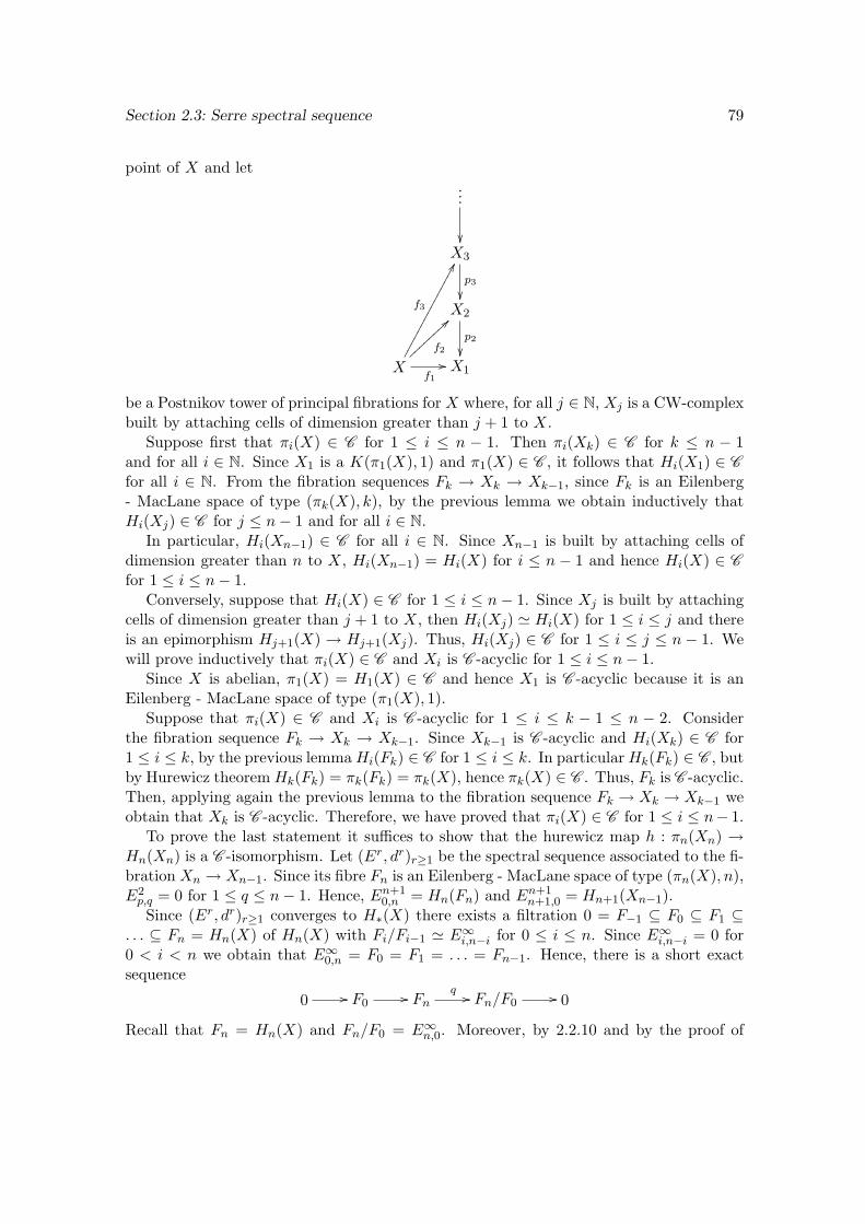
Section 2.3: Serre spectral sequence 79
point of X and let...
X3
p3X2
p2
Xf1//
f2
>>
f3
FFX1
be a Postnikov tower of principal fibrations for X where, for all j ∈ N, Xj is a CW-complexbuilt by attaching cells of dimension greater than j + 1 to X.
Suppose first that πi(X) ∈ C for 1 ≤ i ≤ n − 1. Then πi(Xk) ∈ C for k ≤ n − 1and for all i ∈ N. Since X1 is a K(π1(X), 1) and π1(X) ∈ C , it follows that Hi(X1) ∈ Cfor all i ∈ N. From the fibration sequences Fk → Xk → Xk−1, since Fk is an Eilenberg- MacLane space of type (πk(X), k), by the previous lemma we obtain inductively thatHi(Xj) ∈ C for j ≤ n− 1 and for all i ∈ N.
In particular, Hi(Xn−1) ∈ C for all i ∈ N. Since Xn−1 is built by attaching cells ofdimension greater than n to X, Hi(Xn−1) = Hi(X) for i ≤ n − 1 and hence Hi(X) ∈ Cfor 1 ≤ i ≤ n− 1.
Conversely, suppose that Hi(X) ∈ C for 1 ≤ i ≤ n− 1. Since Xj is built by attachingcells of dimension greater than j + 1 to X, then Hi(Xj) ' Hi(X) for 1 ≤ i ≤ j and thereis an epimorphism Hj+1(X) → Hj+1(Xj). Thus, Hi(Xj) ∈ C for 1 ≤ i ≤ j ≤ n − 1. Wewill prove inductively that πi(X) ∈ C and Xi is C -acyclic for 1 ≤ i ≤ n− 1.
Since X is abelian, π1(X) = H1(X) ∈ C and hence X1 is C -acyclic because it is anEilenberg - MacLane space of type (π1(X), 1).
Suppose that πi(X) ∈ C and Xi is C -acyclic for 1 ≤ i ≤ k − 1 ≤ n − 2. Considerthe fibration sequence Fk → Xk → Xk−1. Since Xk−1 is C -acyclic and Hi(Xk) ∈ C for1 ≤ i ≤ k, by the previous lemmaHi(Fk) ∈ C for 1 ≤ i ≤ k. In particularHk(Fk) ∈ C , butby Hurewicz theoremHk(Fk) = πk(Fk) = πk(X), hence πk(X) ∈ C . Thus, Fk is C -acyclic.Then, applying again the previous lemma to the fibration sequence Fk → Xk → Xk−1 weobtain that Xk is C -acyclic. Therefore, we have proved that πi(X) ∈ C for 1 ≤ i ≤ n− 1.
To prove the last statement it suffices to show that the hurewicz map h : πn(Xn) →Hn(Xn) is a C -isomorphism. Let (Er, dr)r≥1 be the spectral sequence associated to the fi-bration Xn → Xn−1. Since its fibre Fn is an Eilenberg - MacLane space of type (πn(X), n),E2p,q = 0 for 1 ≤ q ≤ n− 1. Hence, En+1
0,n = Hn(Fn) and En+1n+1,0 = Hn+1(Xn−1).
Since (Er, dr)r≥1 converges to H∗(X) there exists a filtration 0 = F−1 ⊆ F0 ⊆ F1 ⊆. . . ⊆ Fn = Hn(X) of Hn(X) with Fi/Fi−1 ' E∞i,n−i for 0 ≤ i ≤ n. Since E∞i,n−i = 0 for0 < i < n we obtain that E∞0,n = F0 = F1 = . . . = Fn−1. Hence, there is a short exactsequence
0 // F0// Fn
q // Fn/F0// 0
Recall that Fn = Hn(X) and Fn/F0 = E∞n,0. Moreover, by 2.2.10 and by the proof of
Section 2.3: Serre spectral sequence 80
2.3.1 we know that F0 is the image of the map Hn(X0n) → Hn(Xn), where (Xi
n)i∈N0 isthe filtration of Xn obtained by taking preimages of the skeletons of Xn−1. But since the0-skeleton of Xn−1 is the base point, it follows that X0
n = Fn. Hence, F0 is the image ofthe map in∗ : Hn(Fn) → Hn(Xn) induced by the inclusion.
It is clear that E∞0,n = En+20,n = coker dn+1
n+1,0 and that En+10,n = Hn(Fn), therefore there
is a short exact sequence
0 // Hn+1(Xn−1)dn+1
n+1,0 // Hn(Fn) // E∞0,n // 0
Combining this short exact sequence with the previous one we obtain an exact sequence
Hn+1(Xn−1)dn+1
n+1,0 // Hn(Fn)inc∗ // Hn(X)
q // E∞n,0 // 0
(note that ker q = F0 = Im (inc∗)).Consider the commutative square
πn(Fn)inc∗ //
h
πn(Xn)
h
Hn(Fn) inc∗// Hn(Xn)
Since πn+1(Xn−1) = 0 and πn(Xn−1) = 0, from the long exact sequence of homotopygroups associated to the fibration Xn → Xn−1 we obtain that the upper map is an iso-morphism. Also, the left-hand vertical map is an isomorphism by the Hurewicz theorem.
Now, if we assume that πi(X) ∈ C for 1 ≤ i ≤ n − 1 then πi(Xn−1) ∈ C for all i ∈ Nand hence, by the first part of this theorem Hi(Xn−1) ∈ C for all i ∈ N. Thus, the firstand fourth terms of the exact sequence above belong to the class C and hence the mapinc∗ : Hn(Fn) → Hn(Xn) is a C -isomorphism.
Therefore, the Hurewicz map h : πn(X) → Hn(X) is a C -isomorphism.
As a first example of application when C is the class of finitely generated abelian groupswe obtain that all the homotopy groups of spheres are finitely generated. However, weshall prove later a much stronger result.
Note also that if C is the class of trivial groups, then we obtain the classical version ofHurewicz Theorem.
Now we turn to the cohomological version of Serre spectral sequence. In this case werequire that π1(B) acts trivially on Hn(F ;G) for all n ∈ N, where this action is definedin a similar way as its homological counterpart.
Theorem 2.3.14. Let f : X → B a Serre fibration with fibre F , where B is a path-connected CW-complex and let G be an abelian group. If π1(B) acts trivially on Hn(F ;G)for all n ∈ N then there exists a cohomological spectral sequence Ep,qr , dr which convergesto H∗(X;G) and such that Ep,q2 ' Hp(B;Hq(F ;G)).
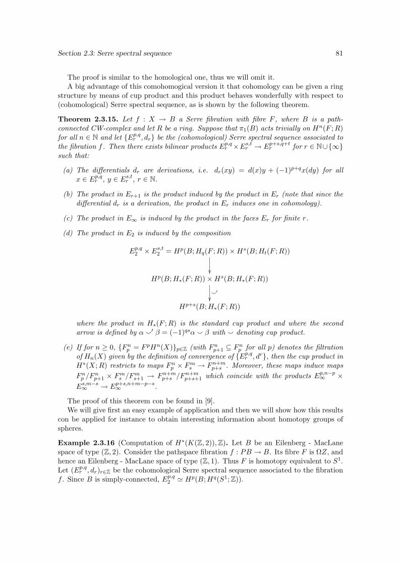
Section 2.3: Serre spectral sequence 81
The proof is similar to the homological one, thus we will omit it.A big advantage of this comohomogical version it that cohomology can be given a ring
structure by means of cup product and this product behaves wonderfully with respect to(cohomological) Serre spectral sequence, as is shown by the following theorem.
Theorem 2.3.15. Let f : X → B a Serre fibration with fibre F , where B is a path-connected CW-complex and let R be a ring. Suppose that π1(B) acts trivially on Hn(F ;R)for all n ∈ N and let Ep,qr , dr be the (cohomological) Serre spectral sequence associated tothe fibration f . Then there exists bilinear products Ep,qr ×Es,tr → Ep+s,q+tr for r ∈ N∪∞such that:
(a) The differentials dr are derivations, i.e. dr(xy) = d(x)y + (−1)p+qx(dy) for allx ∈ Ep,qr , y ∈ Es,tr , r ∈ N.
(b) The product in Er+1 is the product induced by the product in Er (note that since thedifferential dr is a derivation, the product in Er induces one in cohomology).
(c) The product in E∞ is induced by the product in the faces Er for finite r.
(d) The product in E2 is induced by the composition
Ep,q2 × Es,t2 = Hp(B;Hq(F ;R))×Hs(B;Ht(F ;R))
Hp(B;H∗(F ;R))×Hs(B;H∗(F ;R))
`′
Hp+s(B;H∗(F ;R))
where the product in H∗(F ;R) is the standard cup product and where the secondarrow is defined by α `′ β = (−1)qsα ` β with ` denoting cup product.
(e) If for n ≥ 0, Fnp = F pHn(X)p∈Z (with Fnp+1 ⊆ Fnp for all p) denotes the filtrationof Hn(X) given by the definition of convergence of Ep,qr , dr, then the cup product inH∗(X;R) restricts to maps Fnp × Fms → Fn+m
p+s . Moreover, these maps induce mapsFnp /F
np+1 × Fms /F
ms+1 → Fn+m
p+s /Fn+mp+s+1 which coincide with the products Ep,n−p∞ ×
Es,m−s∞ → Ep+s,n+m−p−s∞ .
The proof of this theorem con be found in [9].We will give first an easy example of application and then we will show how this results
con be applied for instance to obtain interesting information about homotopy groups ofspheres.
Example 2.3.16 (Computation of H∗(K(Z, 2)),Z). Let B be an Eilenberg - MacLanespace of type (Z, 2). Consider the pathspace fibration f : PB → B. Its fibre F is ΩZ, andhence an Eilenberg - MacLane space of type (Z, 1). Thus F is homotopy equivalent to S1.Let (Ep,qr , dr)r∈Z be the cohomological Serre spectral sequence associated to the fibrationf . Since B is simply-connected, Ep,q2 ' Hp(B;Hq(S1; Z)).
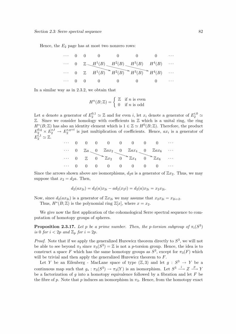
Section 2.3: Serre spectral sequence 82
Hence, the E2 page has at most two nonzero rows:
. . . 0 0 0 0 0 0 . . .
. . . 0 Z++VVVVVVVVVVVVV H1(B)
++WWWWWWWWWWWW H2(B)++WWWWWWWWWWWW H3(B) H4(B) . . .
. . . 0 Z H1(B) H2(B) H3(B) H4(B) . . .
. . . 0 0 0 0 0 0 . . .
In a similar way as in 2.3.2, we obtain that
Hn(B; Z) =
Z if n is even0 if n is odd
Let a denote a generator of E0,12 ' Z and for even i, let xi denote a generator of Ei,02 '
Z. Since we consider homology with coefficients in Z which is a unital ring, the ringH∗(B; Z) has also an identity element which is 1 ∈ Z ' H0(B; Z). Therefore, the productE0,q
2 × Es,t2 → Es,q+t2 is just multiplication of coefficients. Hence, axi is a generator ofEi,12 ' Z.
. . . 0 0 0 0 0 0 0 0 . . .
. . . 0 Za))SSSSSSSS 0 Zax2
**UUUUUUUU 0 Zax4
**UUUUUUUU 0 Zax6. . .
. . . 0 Z 0 Zx2 0 Zx4 0 Zx6. . .
. . . 0 0 0 0 0 0 0 0 . . .
Since the arrows shown above are isomorphisms, d2a is a generator of Zx2. Thus, we maysuppose that x2 = d2a. Then,
d2(ax2i) = d2(a)x2i − ad2(x2i) = d2(a)x2i = x2x2i.
Now, since d2(ax2i) is a generator of Zx2i we may assume that x2x2i = x2i+2.Thus, H∗(B; Z) is the polynomial ring Z[x], where x = x2.
We give now the first application of the cohomological Serre spectral sequence to com-putation of homotopy groups of spheres.
Proposition 2.3.17. Let p be a prime number. Then, the p-torsion subgroup of πi(S3)is 0 for i < 2p and Zp for i = 2p.
Proof. Note that if we apply the generalized Hurewicz theorem directly to S3, we will notbe able to see beyond π3 since π3(S3) = Z is not a p-torsion group. Hence, the idea is toconstruct a space F which has the same homotopy groups as S3, except for π3(F ) whichwill be trivial and then apply the generalized Hurewicz theorem to F .
Let Y be an Eilenberg - MacLane space of type (Z, 3) and let g : S3 → Y be acontinuous map such that g∗ : π3(S3) → π3(Y ) is an isomorphism. Let S3 i−→ Z
p−→ Ybe a factorization of g into a homotopy equivalence followed by a fibration and let F bethe fibre of p. Note that p induces an isomorphism in π3. Hence, from the homotopy exact
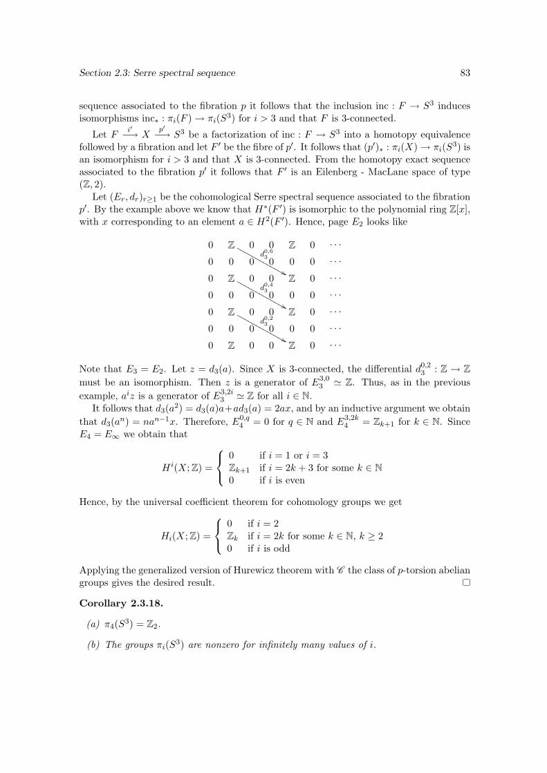
Section 2.3: Serre spectral sequence 83
sequence associated to the fibration p it follows that the inclusion inc : F → S3 inducesisomorphisms inc∗ : πi(F ) → πi(S3) for i > 3 and that F is 3-connected.
Let F i′−→ Xp′−→ S3 be a factorization of inc : F → S3 into a homotopy equivalence
followed by a fibration and let F ′ be the fibre of p′. It follows that (p′)∗ : πi(X) → πi(S3) isan isomorphism for i > 3 and that X is 3-connected. From the homotopy exact sequenceassociated to the fibration p′ it follows that F ′ is an Eilenberg - MacLane space of type(Z, 2).
Let (Er, dr)r≥1 be the cohomological Serre spectral sequence associated to the fibrationp′. By the example above we know that H∗(F ′) is isomorphic to the polynomial ring Z[x],with x corresponding to an element a ∈ H2(F ′). Hence, page E2 looks like
0 Zd0,63
&&MMMMMMMMMMMMM 0 0 Z 0 . . .
0 0 0 0 0 0 . . .
0 Zd0,43
&&MMMMMMMMMMMMM 0 0 Z 0 . . .
0 0 0 0 0 0 . . .
0 Zd0,23
&&MMMMMMMMMMMMM 0 0 Z 0 . . .
0 0 0 0 0 0 . . .
0 Z 0 0 Z 0 . . .
Note that E3 = E2. Let z = d3(a). Since X is 3-connected, the differential d0,23 : Z → Z
must be an isomorphism. Then z is a generator of E3,03 ' Z. Thus, as in the previous
example, aiz is a generator of E3,2i3 ' Z for all i ∈ N.
It follows that d3(a2) = d3(a)a+ad3(a) = 2ax, and by an inductive argument we obtainthat d3(an) = nan−1x. Therefore, E0,q
4 = 0 for q ∈ N and E3,2k4 = Zk+1 for k ∈ N. Since
E4 = E∞ we obtain that
H i(X; Z) =
0 if i = 1 or i = 3Zk+1 if i = 2k + 3 for some k ∈ N0 if i is even
Hence, by the universal coefficient theorem for cohomology groups we get
Hi(X; Z) =
0 if i = 2Zk if i = 2k for some k ∈ N, k ≥ 20 if i is odd
Applying the generalized version of Hurewicz theorem with C the class of p-torsion abeliangroups gives the desired result.
Corollary 2.3.18.
(a) π4(S3) = Z2.
(b) The groups πi(S3) are nonzero for infinitely many values of i.
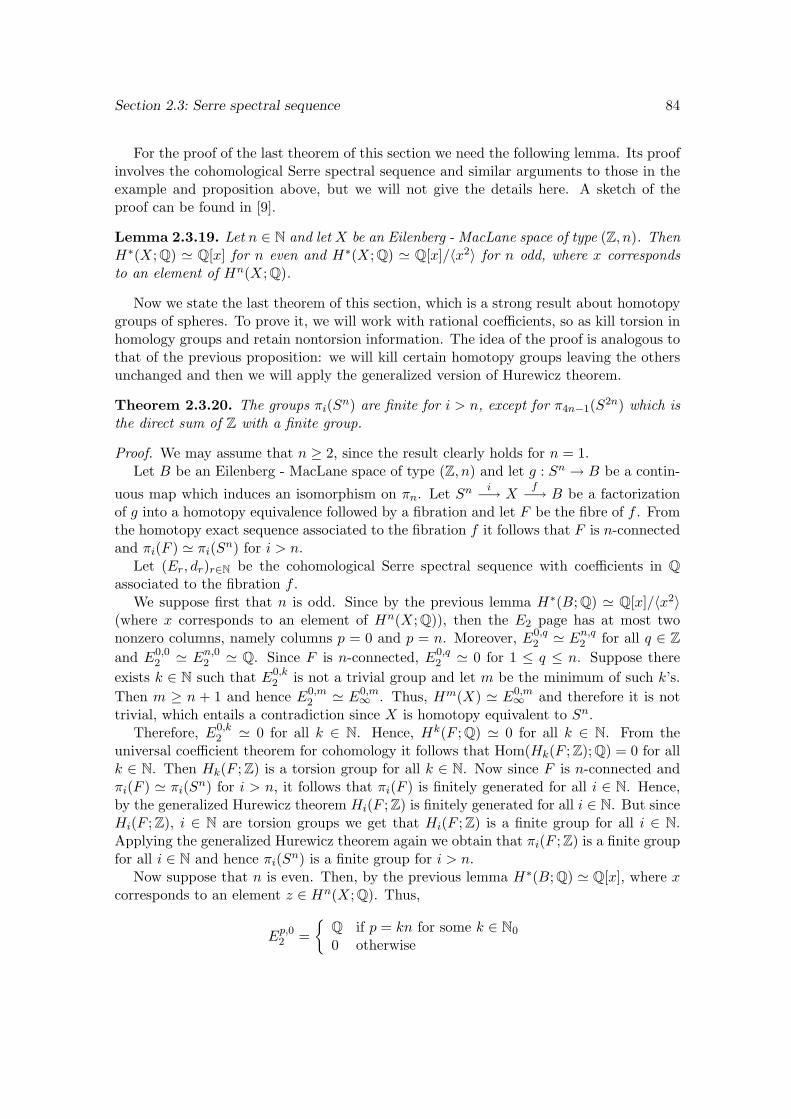
Section 2.3: Serre spectral sequence 84
For the proof of the last theorem of this section we need the following lemma. Its proofinvolves the cohomological Serre spectral sequence and similar arguments to those in theexample and proposition above, but we will not give the details here. A sketch of theproof can be found in [9].
Lemma 2.3.19. Let n ∈ N and let X be an Eilenberg - MacLane space of type (Z, n). ThenH∗(X; Q) ' Q[x] for n even and H∗(X; Q) ' Q[x]/〈x2〉 for n odd, where x correspondsto an element of Hn(X; Q).
Now we state the last theorem of this section, which is a strong result about homotopygroups of spheres. To prove it, we will work with rational coefficients, so as kill torsion inhomology groups and retain nontorsion information. The idea of the proof is analogous tothat of the previous proposition: we will kill certain homotopy groups leaving the othersunchanged and then we will apply the generalized version of Hurewicz theorem.
Theorem 2.3.20. The groups πi(Sn) are finite for i > n, except for π4n−1(S2n) which isthe direct sum of Z with a finite group.
Proof. We may assume that n ≥ 2, since the result clearly holds for n = 1.Let B be an Eilenberg - MacLane space of type (Z, n) and let g : Sn → B be a contin-
uous map which induces an isomorphism on πn. Let Sn i−→ Xf−→ B be a factorization
of g into a homotopy equivalence followed by a fibration and let F be the fibre of f . Fromthe homotopy exact sequence associated to the fibration f it follows that F is n-connectedand πi(F ) ' πi(Sn) for i > n.
Let (Er, dr)r∈N be the cohomological Serre spectral sequence with coefficients in Qassociated to the fibration f .
We suppose first that n is odd. Since by the previous lemma H∗(B; Q) ' Q[x]/〈x2〉(where x corresponds to an element of Hn(X; Q)), then the E2 page has at most twononzero columns, namely columns p = 0 and p = n. Moreover, E0,q
2 ' En,q2 for all q ∈ Zand E0,0
2 ' En,02 ' Q. Since F is n-connected, E0,q2 ' 0 for 1 ≤ q ≤ n. Suppose there
exists k ∈ N such that E0,k2 is not a trivial group and let m be the minimum of such k’s.
Then m ≥ n + 1 and hence E0,m2 ' E0,m
∞ . Thus, Hm(X) ' E0,m∞ and therefore it is not
trivial, which entails a contradiction since X is homotopy equivalent to Sn.Therefore, E0,k
2 ' 0 for all k ∈ N. Hence, Hk(F ; Q) ' 0 for all k ∈ N. From theuniversal coefficient theorem for cohomology it follows that Hom(Hk(F ; Z); Q) = 0 for allk ∈ N. Then Hk(F ; Z) is a torsion group for all k ∈ N. Now since F is n-connected andπi(F ) ' πi(Sn) for i > n, it follows that πi(F ) is finitely generated for all i ∈ N. Hence,by the generalized Hurewicz theorem Hi(F ; Z) is finitely generated for all i ∈ N. But sinceHi(F ; Z), i ∈ N are torsion groups we get that Hi(F ; Z) is a finite group for all i ∈ N.Applying the generalized Hurewicz theorem again we obtain that πi(F ; Z) is a finite groupfor all i ∈ N and hence πi(Sn) is a finite group for i > n.
Now suppose that n is even. Then, by the previous lemma H∗(B; Q) ' Q[x], where xcorresponds to an element z ∈ Hn(X; Q). Thus,
Ep,02 =
Q if p = kn for some k ∈ N0
0 otherwise
Section 2.4: Localization of CW-complexes 85
Since F is n-connected, E0,q2 ' 0 for 1 ≤ q ≤ n. Suppose that E0,q
2 is not trivial forsome q < 2n − 1 and let m be the minimum q with this property. Then m > n andE0,m∞ ' E0,m
2 . Hence Hm(X; Q) is not trivial, but X is homotopy equivalent to Sn, whichentails a contradiction. Hence, Hq(F ; Q) ' E0,q
2 ' 0 for 1 ≤ q < 2n − 1. Then Ep,q2 ' 0for 1 ≤ q < 2n− 1 and for all p ∈ N.
In consequence, E0,2n−1n ' E0,2n−1
2 , E2n,0n ' E2n,0
2 ' Q and the differential d0,2n−12n :
E0,2n−1n → E2n,0
n ' Q must be an isomorphism because otherwise either E0,2n−1∞ or E2n,0
∞would be nontrivial. Hence we have that H2n−1(F ; Q) ' Q and Hq(F ; Q) ' 0 for 1 ≤ q <2n − 1. From the universal coefficient theorem for cohomology, since Hi(F ; Z) is finitelygenerated for all i ∈ N, by an inductive argument and proceeding as in the case above itis not difficult to prove that Hi(F ; Z) is a finite group for 1 ≤ i < 2n− 1 and H2n−1(F ; Z)is the direct sum of Z with a finite group. Applying the generalized Hurewicz theoremwith C the class of finite groups we obtain that the same holds for the groups πi(F ),1 ≤ i ≤ 2n− 1. Therefore, πi(Sn) is a finite group for 1 ≤ i < 2n− 1 and π2n−1(F ; Z) isthe direct sum of Z with a finite group.
Now, let a ∈ E0,2n−1n be such that dn(a) = z2 ∈ E2n,0
n ' H2n(X; Q). Thus, by thederivation property dni,2n−1
n (azi) = zi+2 for i ∈ N. Then dni,2n−1n is an isomorphism for
all i ∈ N. With a similar argument as in the previous case we obtain that E0,k2 ' 0 for all
k ≥ 2n, since the first nontrivial entry would survive to E∞. Thus, H∗(F ; Q) ' Q[x]/〈x2〉,where x corresponds to an element of H2n−1(X; Q).
Let F ′ be obtained from F by attaching cells of dimension greater than 2n − 1 andsuch that πi(F ′) = 0 for i ≥ 2n − 1. Let inc : F → F ′ denote the inclusion map and
let F i′−→ X ′f ′−→ F ′ be a factorization of inc into a homotopy equivalence followed by a
fibration. Let F ′′ be the fibre of f ′. From the homotopy exact sequence for the fibrationf ′ it follows that πi(F ′′) ' πi(F ) ' πi(Sn) for i ≥ 2n− 1.
Since F ′ has finite homotopy groups, the same holds for its reduced homology groupsand hence Hn(F ′,Q) ' 0 for n ∈ N. From the cohomological Serre spectral sequence forthe fibration f ′ we obtain that H∗(F ′′; Q) ' H∗(X ′; Q) ' H∗(F ; Q) ' Q[x]/〈x2〉, wherex corresponds to an element of H2n−1(F ′′; Q).
Let Y be an Eilenberg - MacLane space of type (Z, 2n− 1) and let F ′′ → Y be a mapinducing an isomorphism on the nontorsion in π2n−1. Now, we consider factorization ofthis map into a homotopy equivalence followed by a fibration and with a similar argumentas in the case n odd we obtain that πi(F ′′) ' πi(Sn) is finite for i > 2n− 1.
2.4 Localization of CW-complexes
In this section we will study localization of CW-complexes. We begin by recalling somebasic facts about algebraic localization of rings and modules.
For the whole section, P will denote a subset of the set of prime numbers. If G is anabelian group and a ∈ Z, we denote by µa : G→ G the group homomorphism defined byµa(g) = ag.
We denoteZP =
ab∈ Q / (b : p) = 1 for all p ∈ P
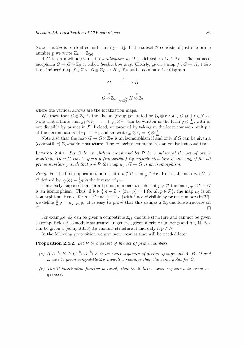
Section 2.4: Localization of CW-complexes 86
Note that ZP is torsionfree and that Z∅ = Q. If the subset P consists of just one primenumber p we write ZP = Z(p).
If G is an abelian group, its localization at P is defined as G ⊗ ZP . The inducedmorphism G→ G⊗ ZP is called localization map. Clearly, given a map f : G→ H, thereis an induced map f ⊗ ZP : G⊗ ZP → H ⊗ ZP and a commutative diagram
Gf //
H
G⊗ ZP f⊗ZP
// H ⊗ ZP
where the vertical arrows are the localization maps.We know that G⊗ ZP is the abelian group generated by g ⊗ r / g ∈ G and r ∈ ZP.
Note that a finite sum g1 ⊗ r1 + . . . + gn ⊗ rn can be written in the form g ⊗ 1m , with m
not divisible by primes in P. Indeed, we proceed by taking m the least common multipleof the denominators of r1, . . . , rn and we write gi ⊗ ri = g′i ⊗ 1
m .Note also that the map G→ G⊗ZP is an isomorphism if and only if G can be given a
(compatible) ZP -module structure. The following lemma states an equivalent condition.
Lemma 2.4.1. Let G be an abelian group and let P be a subset of the set of primenumbers. Then G can be given a (compatible) ZP-module structure if and only if for allprime numbers p such that p /∈ P the map µp : G→ G is an isomorphism.
Proof. For the first implication, note that if p /∈ P then 1p ∈ ZP . Hence, the map νp : G→
G defined by νp(g) = 1pg is the inverse of µp.
Conversely, suppose that for all prime numbers p such that p /∈ P the map µp : G→ Gis an isomorphism. Thus, if b ∈ m ∈ Z / (m : p) = 1 for all p ∈ P, the map µb is anisomorphism. Hence, for g ∈ G and a
b ∈ ZP (with b not divisible by prime numbers in P),we define a
b .g = µ−1b µag. It is easy to prove that this defines a ZP -module structure on
G.
For example, Z3 can be given a compatible Z(3)-module structure and can not be givena (compatible) Z(2)-module structure. In general, given a prime number p and n ∈ N, Zpn
can be given a (compatible) ZP -module structure if and only if p ∈ P.In the following proposition we give some results that will be needed later.
Proposition 2.4.2. Let P be a subset of the set of prime numbers.
(a) If Af→ B
g→ Ch→ D
k→ E is an exact sequence of abelian groups and A, B, D andE can be given compatible ZP-module structures then the same holds for C.
(b) The P-localization functor is exact, that is, it takes exact sequences to exact se-quences.
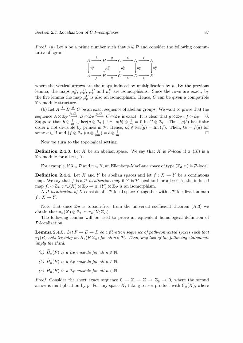
Section 2.4: Localization of CW-complexes 87
Proof. (a) Let p be a prime number such that p /∈ P and consider the following commu-tative diagram
Af //
µAp
Bg //
µBp
Ch //
µCp
Dk //
µDp
E
µEp
A
f// B g
// Ch// D
k// E
where the vertical arrows are the maps induced by multiplication by p. By the previouslemma, the maps µAp , µBp , µDp and µEp are isomorphisms. Since the rows are exact, bythe five lemma the map µCp is also an isomorphism. Hence, C can be given a compatibleZP -module structure.
(b) Let Af→ B
g→ C be an exact sequence of abelian groups. We want to prove that the
sequence A⊗ZPf⊗ZP−→ B⊗ZP
g⊗ZP−→ C ⊗ZP is exact. It is clear that g⊗ZP f ⊗ZP = 0.Suppose that b ⊗ 1
m ∈ ker(g ⊗ ZP), i.e. g(b) ⊗ 1m = 0 in C ⊗ ZP . Thus, g(b) has finite
order k not divisible by primes in P. Hence, kb ∈ ker(g) = Im (f). Then, kb = f(a) forsome a ∈ A and (f ⊗ ZP)(a⊗ 1
km) = b⊗ 1m .
Now we turn to the topological setting.
Definition 2.4.3. Let X be an abelian space. We say that X is P-local if πn(X) is aZP -module for all n ∈ N.
For example, if 3 ∈ P and n ∈ N, an Eilenberg-MacLane space of type (Z3, n) is P-local.
Definition 2.4.4. Let X and Y be abelian spaces and let f : X → Y be a continuousmap. We say that f is a P-localization map if Y is P-local and for all n ∈ N, the inducedmap f∗ ⊗ ZP : πn(X)⊗ ZP → πn(Y )⊗ ZP is an isomorphism.
A P-localization of X consists of a P-local space Y together with a P-localization mapf : X → Y .
Note that since ZP is torsion-free, from the universal coefficient theorem (A.3) weobtain that πn(X)⊗ ZP ' πn(X; ZP).
The following lemma will be used to prove an equivalent homological definition ofP-localization.
Lemma 2.4.5. Let F → E → B be a fibration sequence of path-connected spaces such thatπ1(B) acts trivially on H∗(F,Zp) for all p /∈ P. Then, any two of the following statementsimply the third.
(a) Hn(F ) is a ZP-module for all n ∈ N.
(b) Hn(E) is a ZP-module for all n ∈ N.
(c) Hn(B) is a ZP-module for all n ∈ N.
Proof. Consider the short exact sequence 0 → Z → Z → Zp → 0, where the secondarrow is multiplication by p. For any space X, taking tensor product with Cn(X), where
Section 2.4: Localization of CW-complexes 88
(C∗(X), d) is the singular chain complex of X, we obtain a short exact sequence of chaincomplexes, which induces a long exact sequence
. . . // Hn(X,Z)µp // Hn(X,Z) // Hn(X,Zp) // Hn−1(X,Z)
µp // Hn−1(X,Z) // . . .
Hence, applying 2.4.1 we obtain that Hn(X) is a ZP -module for all n ∈ N if and only ifHn(X,Zp) = 0 for all n ∈ N and for all prime numbers p /∈ P.
The result then follows from the Serre spectral sequence.
Proposition 2.4.6. Let X and Y be abelian spaces and let f : X → Y be a P-localizationmap. Then for all n ∈ N, Hn(Y ) can be given a compatible ZP-module structure and theinduced map f∗ ⊗ ZP : Hn(X)⊗ ZP → Hn(Y )⊗ ZP is an isomorphism.
Proof. We consider first the particular case in which X is an Eilenberg - MacLane spaceof type (G,n). Hence, Y is an Eilenberg - MacLane space of type (G⊗ ZP , n).
We proceed by induction on n, starting with the case n = 1. If G = Z then Y is anEilenberg - MacLane space of type (ZP , 1). But a Moore space of type (ZP , 1) can beconstructed as a mapping telescope of a sequence of maps S2 → S2 of appropiate degrees,as in [8], p. 312. From this construction it is not difficult to verify that a Moore space oftype (ZP , 1) is also an Eilenberg - MacLane space of type (ZP , 1). Hence, Y is a Moorespace of type (ZP , 1) and thus, for all n ∈ N, Hn(Y ) can be given a compatible ZP -modulestructure.
The naturality of the Hurewicz map gives us a commutative square
π1(X)⊗ ZPf∗⊗ZP //
h⊗ZP
π1(Y )⊗ ZPh⊗ZP
H1(X)⊗ ZPf∗⊗ZP
// H1(Y )⊗ ZP
The vertical arrows are the abelianization maps, and hence isomorphisms in this case.The upper arrow is also an isomorphism since f : X → Y is a P-localization map. Thus,f∗ ⊗ ZP : Hn(X)⊗ ZP → Hn(Y )⊗ ZP is an isomorphism.
If G = Zpm with p /∈ P and m ∈ N then G ⊗ ZP = G. Since f : X → Y induces anisomorphism on π1 and X and Y are Eilenberg - MacLane space of type (G,n) it followsthat f is a homotopy equivalence. Hence, the result holds in this case.
If G = Zpm with p ∈ P and m ∈ N then G⊗ ZP = 0. Hence, Y is contractible and theresult follows.
If G is finitely generated, the result follows from the cases above applying the Kunnethformula (A.11).
For an arbitrary group G, we know that G is the direct limit of its finitely generatedsubgroups. Hence, the result holds since homology commutes with direct limits.
Now suppose that n ≥ 2 and that the statement holds for n− 1. Consider the commu-tative diagram
ΩX //
PX //
X
ΩY // PY // Y
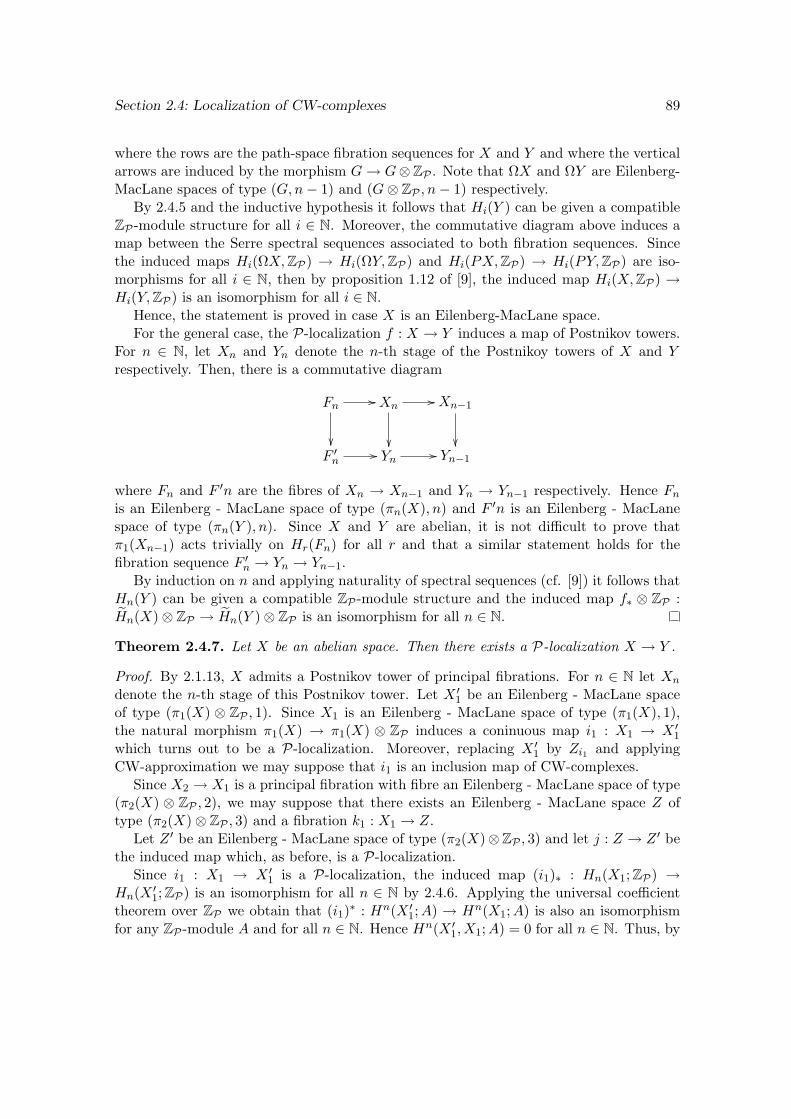
Section 2.4: Localization of CW-complexes 89
where the rows are the path-space fibration sequences for X and Y and where the verticalarrows are induced by the morphism G→ G⊗ZP . Note that ΩX and ΩY are Eilenberg-MacLane spaces of type (G,n− 1) and (G⊗ ZP , n− 1) respectively.
By 2.4.5 and the inductive hypothesis it follows that Hi(Y ) can be given a compatibleZP -module structure for all i ∈ N. Moreover, the commutative diagram above induces amap between the Serre spectral sequences associated to both fibration sequences. Sincethe induced maps Hi(ΩX,ZP) → Hi(ΩY,ZP) and Hi(PX,ZP) → Hi(PY,ZP) are iso-morphisms for all i ∈ N, then by proposition 1.12 of [9], the induced map Hi(X,ZP) →Hi(Y,ZP) is an isomorphism for all i ∈ N.
Hence, the statement is proved in case X is an Eilenberg-MacLane space.For the general case, the P-localization f : X → Y induces a map of Postnikov towers.
For n ∈ N, let Xn and Yn denote the n-th stage of the Postnikoy towers of X and Yrespectively. Then, there is a commutative diagram
Fn //
Xn//
Xn−1
F ′n
// Yn // Yn−1
where Fn and F ′n are the fibres of Xn → Xn−1 and Yn → Yn−1 respectively. Hence Fnis an Eilenberg - MacLane space of type (πn(X), n) and F ′n is an Eilenberg - MacLanespace of type (πn(Y ), n). Since X and Y are abelian, it is not difficult to prove thatπ1(Xn−1) acts trivially on Hr(Fn) for all r and that a similar statement holds for thefibration sequence F ′n → Yn → Yn−1.
By induction on n and applying naturality of spectral sequences (cf. [9]) it follows thatHn(Y ) can be given a compatible ZP -module structure and the induced map f∗ ⊗ ZP :Hn(X)⊗ ZP → Hn(Y )⊗ ZP is an isomorphism for all n ∈ N.
Theorem 2.4.7. Let X be an abelian space. Then there exists a P-localization X → Y .
Proof. By 2.1.13, X admits a Postnikov tower of principal fibrations. For n ∈ N let Xn
denote the n-th stage of this Postnikov tower. Let X ′1 be an Eilenberg - MacLane spaceof type (π1(X) ⊗ ZP , 1). Since X1 is an Eilenberg - MacLane space of type (π1(X), 1),the natural morphism π1(X) → π1(X) ⊗ ZP induces a coninuous map i1 : X1 → X ′1which turns out to be a P-localization. Moreover, replacing X ′1 by Zi1 and applyingCW-approximation we may suppose that i1 is an inclusion map of CW-complexes.
Since X2 → X1 is a principal fibration with fibre an Eilenberg - MacLane space of type(π2(X) ⊗ ZP , 2), we may suppose that there exists an Eilenberg - MacLane space Z oftype (π2(X)⊗ ZP , 3) and a fibration k1 : X1 → Z.
Let Z ′ be an Eilenberg - MacLane space of type (π2(X)⊗ZP , 3) and let j : Z → Z ′ bethe induced map which, as before, is a P-localization.
Since i1 : X1 → X ′1 is a P-localization, the induced map (i1)∗ : Hn(X1; ZP) →Hn(X ′1; ZP) is an isomorphism for all n ∈ N by 2.4.6. Applying the universal coefficienttheorem over ZP we obtain that (i1)∗ : Hn(X ′1;A) → Hn(X1;A) is also an isomorphismfor any ZP -module A and for all n ∈ N. Hence Hn(X ′1, X1;A) = 0 for all n ∈ N. Thus, by
Section 2.4: Localization of CW-complexes 90
obstruction theory, the composition jk1 : X1 → Z ′ can be extended to a continuous mapk′1 : X ′1 → Z ′.
We may suppose that k′1 is a fibration by writing it as a composition of a homotopyequivalence with a fibration. Let X ′2 be the fibre of k′1 and let i2 : X2 → X ′2 be theinduced map. Note that π1(X ′2) is abelian and that X ′2 admits a Postnikov tower ofprincipal fibrations by construction. Hence, by 2.1.13 we obtain that X ′2 is abelian. Also,from the long exact sequence of homotopy groups associated to the fibration k′1 : X ′1 → Z ′
and applying 2.4.2 we conclude that X ′2 is P-local. Also, from the five-lemma and item(b) of 2.4.2 it follows that i2 : X2 → X ′2 is a P-localization.
Hence, we may construct inductively a Postnikov tower of principal fibrations X ′n →X ′n−1 together with P-localizations in : Xn → X ′n. Let X ′ be a CW-approximation tolim←−
X ′n. Since by 2.1.14 there is a weak equivalence X → lim←−
X ′n, we obtain the desired
P-localization X → lim←−
X ′n → X ′.
Now we can complete the equivalent homological definition of localization with thefollowing theorem. Note that it aids us in checking that a map is a P-isomorphism, sinceit is often easier to work with homology groups than with homotopy groups.
Theorem 2.4.8. Let X and Y be abelian spaces and let f : X → Y be a continuousmap. Then f is a P-localization map if and only if for all n ∈ N, Hn(Y ) can be given acompatible ZP-module structure and the induced map f∗⊗ZP : Hn(X)⊗ZP → Hn(Y )⊗ZPis an isomorphism.
Proof. The first implication is proposition 2.4.6. For the converse, let X → X ′ be aP-localization of X. We may suppose that (Y,X) is a CW-pair, changing Y by Zfand then taking a CW-approximation. Hence, Hn(Y,X,ZP) = 0 for all n ∈ N, andthus Hn(Y,X,ZP) = 0 for all n ∈ N by the universal coefficient theorem over ZP . Byobstruction theory, the P-localization map X → X ′ can be extended to g : Y → X ′.
By the first implication, Hn(X ′) can be given a compatible ZP -module structure andthe induced map Hn(X; ZP) → Hn(X ′;ZP) is an isomorphism. Hence, the induced mapg∗ : Hn(Y ; ZP) → Hn(X ′;ZP) is also an isomorphism. But since Hn(Y ; ZP) ' Hn(Y )and Hn(X ′; ZP) ' Hn(X ′) for all n ∈ N we obtain that g∗ : Hn(Y ) → Hn(X ′) is anisomorphism for all n ∈ N.
Since Y and X are abelian, applying 1.4.36 we get that g : Y → X ′ is a homotopyequivalence. Thus, X → Y is a P-localization map.
Proposition 2.4.9. Let f : X → Y and f ′ : X ′ → Y ′ be P-localizations and let g :X → X ′ be a continuous map. Then, there exists a continuous map h : Y → Y ′ suchthat hf = f ′g. Moreover, if g′ : X → X ′ and h′ : Y → Y ′ are continuous maps such thath′f = f ′g′ and g ' g′ then h ' h′.
The proof of this proposition involves obstruction theory and similar arguments as thoseabove and will not be given here. From it we obtain the following important corollary.
Corollary 2.4.10. Let X be an abelian space. Then the P-localization of X is uniqueup to homotopy equivalence, i.e. given P-localizations f : X → Y and f ′ : X → Y ′ thereexists a homotopy equivalence h : Y → Y ′ such that hf = f ′.
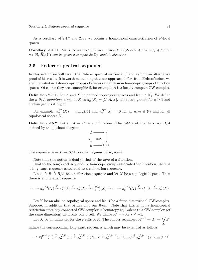
Section 2.5: Federer spectral sequence 91
As a corollary of 2.4.7 and 2.4.9 we obtain a homological caracterization of P-localspaces.
Corollary 2.4.11. Let X be an abelian space. Then X is P-local if and only if for alln ∈ N, Hn(Y ) can be given a compatible ZP-module structure.
2.5 Federer spectral sequence
In this section we will recall the Federer spectral sequence [6] and exhibit an alternativeproof of his result. It is worth mentioning that our approach differs from Federer’s since weare interested in A-homotopy groups of spaces rather than in homotopy groups of functionspaces. Of course they are isomorphic if, for example, A is a locally compact CW-complex.
Definition 2.5.1. Let A and X be pointed topological spaces and let n ∈ N0. We definethe n-th A-homotopy group of X as πAn (X) = [ΣnA,X]. These are groups for n ≥ 1 andabelian groups if n ≥ 2.
For example, πSm
n (X) = πn+m(X) and πDm
n (X) = 0 for all n,m ∈ N0 and for alltopological spaces X.
Definition 2.5.2. Let i : A → B be a cofibration. The cofibre of i is the space B/Adefined by the pushout diagram
A //
i
push
∗
B // B/A
The sequence A→ B → B/A is called cofibration sequence.
Note that this notion is dual to that of the fibre of a fibration.Dual to the long exact sequence of homotopy groups associated the fibration, there is
a long exact sequence associated to a cofibration sequence.Let A i→ B
q→ B/A be a cofibration sequence and let X be a topological space. Thenthere is a long exact sequence
. . . // πB/An (X)
q∗ // πBn (X) i∗ // πAn (X) ∂ // πB/An−1 (X) // . . . // π
B/A0 (X)
q∗ // πB0 (X) i∗ // πA0 (X)
Let Y be an abelian topological space and let A be a finite dimensional CW-complex.Suppose, in addition that A has only one 0-cell. Note that this is not a homotopicalrestriction since any connected CW-complex is homotopy equivalent to a CW-complex (ofthe same dimension) with only one 0-cell. We define Ar = ∗ for r ≤ −1.
Let Jr be an index set for the r-cells of A. The cofiber sequences Ar−1 → Ar →∨Jr
Sr
induce the corresponding long exact sequences which may be extended as follows
. . . // πAr−1
1 (Y )∂ // π
WSr
0 (Y )q // π
WSr
0 (Y )/Im ∂0 // π
WSr−1
0 (Y )/Im ∂id // π
WSr−1
0 (Y )/Im ∂ // 0
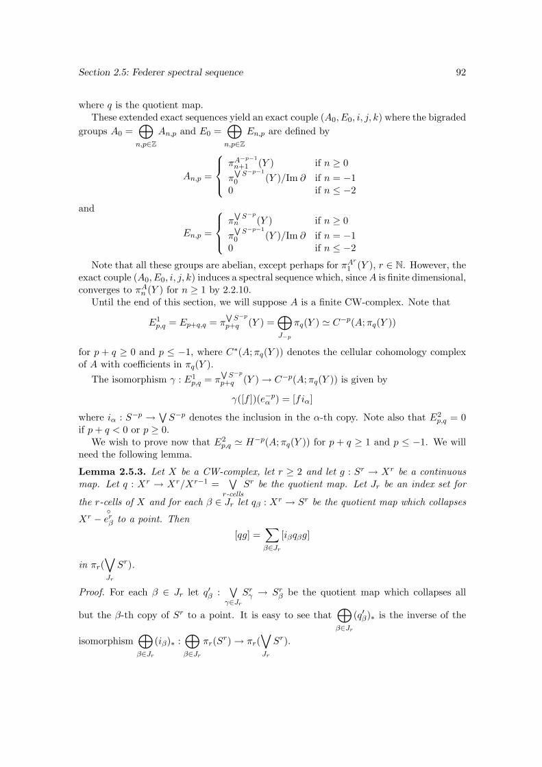
Section 2.5: Federer spectral sequence 92
where q is the quotient map.These extended exact sequences yield an exact couple (A0, E0, i, j, k) where the bigraded
groups A0 =⊕n,p∈Z
An,p and E0 =⊕n,p∈Z
En,p are defined by
An,p =
πA
−p−1
n+1 (Y ) if n ≥ 0π
WS−p−1
0 (Y )/Im ∂ if n = −10 if n ≤ −2
and
En,p =
π
WS−p
n (Y ) if n ≥ 0π
WS−p−1
0 (Y )/Im ∂ if n = −10 if n ≤ −2
Note that all these groups are abelian, except perhaps for πAr
1 (Y ), r ∈ N. However, theexact couple (A0, E0, i, j, k) induces a spectral sequence which, sinceA is finite dimensional,converges to πAn (Y ) for n ≥ 1 by 2.2.10.
Until the end of this section, we will suppose A is a finite CW-complex. Note that
E1p,q = Ep+q,q = π
WS−p
p+q (Y ) =⊕J−p
πq(Y ) ' C−p(A;πq(Y ))
for p + q ≥ 0 and p ≤ −1, where C∗(A;πq(Y )) denotes the cellular cohomology complexof A with coefficients in πq(Y ).
The isomorphism γ : E1p,q = π
WS−p
p+q (Y ) → C−p(A;πq(Y )) is given by
γ([f ])(e−pα ) = [fiα]
where iα : S−p →∨S−p denotes the inclusion in the α-th copy. Note also that E2
p,q = 0if p+ q < 0 or p ≥ 0.
We wish to prove now that E2p,q ' H−p(A;πq(Y )) for p + q ≥ 1 and p ≤ −1. We will
need the following lemma.
Lemma 2.5.3. Let X be a CW-complex, let r ≥ 2 and let g : Sr → Xr be a continuousmap. Let q : Xr → Xr/Xr−1 =
∨r-cells
Sr be the quotient map. Let Jr be an index set for
the r-cells of X and for each β ∈ Jr let qβ : Xr → Sr be the quotient map which collapses
Xr −erβ to a point. Then
[qg] =∑β∈Jr
[iβqβg]
in πr(∨Jr
Sr).
Proof. For each β ∈ Jr let q′β :∨γ∈Jr
Srγ → Srβ be the quotient map which collapses all
but the β-th copy of Sr to a point. It is easy to see that⊕β∈Jr
(q′β)∗ is the inverse of the
isomorphism⊕β∈Jr
(iβ)∗ :⊕β∈Jr
πr(Sr) → πr(∨Jr
Sr).
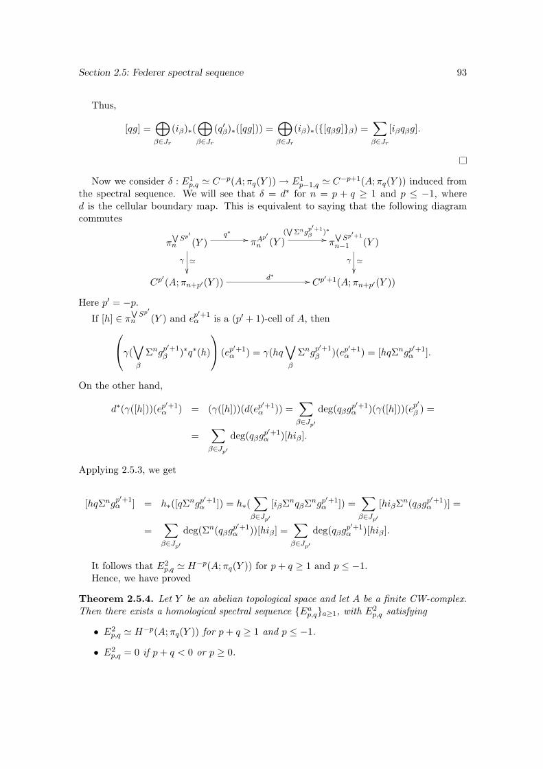
Section 2.5: Federer spectral sequence 93
Thus,
[qg] =⊕β∈Jr
(iβ)∗(⊕β∈Jr
(q′β)∗([qg])) =⊕β∈Jr
(iβ)∗([qβg]β) =∑β∈Jr
[iβqβg].
Now we consider δ : E1p,q ' C−p(A;πq(Y )) → E1
p−1,q ' C−p+1(A;πq(Y )) induced fromthe spectral sequence. We will see that δ = d∗ for n = p + q ≥ 1 and p ≤ −1, whered is the cellular boundary map. This is equivalent to saying that the following diagramcommutes
πWSp′
n (Y )q∗ //
'γ
πAp′
n (Y )(W
Σngp′+1β )∗
// πWSp′+1
n−1 (Y )
'γ
Cp
′(A;πn+p′(Y )) d∗ // Cp
′+1(A;πn+p′(Y ))
Here p′ = −p.If [h] ∈ π
WSp′
n (Y ) and ep′+1α is a (p′ + 1)-cell of A, thenγ(∨
β
Σngp′+1β )∗q∗(h)
(ep′+1α ) = γ(hq
∨β
Σngp′+1β )(ep
′+1α ) = [hqΣngp
′+1α ].
On the other hand,
d∗(γ([h]))(ep′+1α ) = (γ([h]))(d(ep
′+1α )) =
∑β∈Jp′
deg(qβgp′+1α )(γ([h]))(ep
′
β ) =
=∑β∈Jp′
deg(qβgp′+1α )[hiβ].
Applying 2.5.3, we get
[hqΣngp′+1α ] = h∗([qΣngp
′+1α ]) = h∗(
∑β∈Jp′
[iβΣnqβΣngp′+1α ]) =
∑β∈Jp′
[hiβΣn(qβgp′+1α )] =
=∑β∈Jp′
deg(Σn(qβgp′+1α ))[hiβ] =
∑β∈Jp′
deg(qβgp′+1α )[hiβ].
It follows that E2p,q ' H−p(A;πq(Y )) for p+ q ≥ 1 and p ≤ −1.
Hence, we have proved
Theorem 2.5.4. Let Y be an abelian topological space and let A be a finite CW-complex.Then there exists a homological spectral sequence Eap,qa≥1, with E2
p,q satisfying
• E2p,q ' H−p(A;πq(Y )) for p+ q ≥ 1 and p ≤ −1.
• E2p,q = 0 if p+ q < 0 or p ≥ 0.
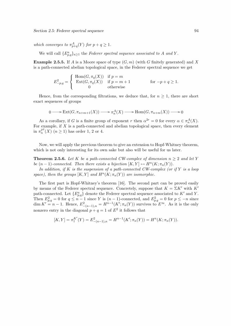
Section 2.5: Federer spectral sequence 94
which converges to πAp+q(Y ) for p+ q ≥ 1.
We will call Eap,qa≥1 the Federer spectral sequence associated to A and Y .
Example 2.5.5. If A is a Moore space of type (G,m) (with G finitely generated) and Xis a path-connected abelian topological space, in the Federer spectral sequence we get
E2−p,q =
Hom(G, πq(X)) if p = mExt(G, πq(X)) if p = m+ 1
0 otherwisefor −p+ q ≥ 1.
Hence, from the corresponding filtrations, we deduce that, for n ≥ 1, there are shortexact sequences of groups
0 // Ext(G, πn+m+1(X)) // πAn (X) // Hom(G, πn+m(X)) // 0
As a corollary, if G is a finite group of exponent r then α2r = 0 for every α ∈ πAn (X).For example, if X is a path-connected and abelian topological space, then every elementin πP2
n (X) (n ≥ 1) has order 1, 2 or 4.
Now, we will apply the previous theorem to give an extension to Hopf-Whitney theorem,which is not only interesting for its own sake but also will be useful for us later.
Theorem 2.5.6. Let K be a path-connected CW-complex of dimension n ≥ 2 and let Ybe (n− 1)-connected. Then there exists a bijection [K,Y ] ↔ Hn(K;πn(Y )).
In addition, if K is the suspension of a path-connected CW-complex (or if Y is a loopspace), then the groups [K,Y ] and Hn(K;πn(Y )) are isomorphic.
The first part is Hopf-Whitney’s theorem [16]. The second part can be proved easilyby means of the Federer spectral sequence. Concretely, suppose that K = ΣK ′ with K ′
path-connected. Let Eap,q denote the Federer spectral sequence associated to K ′ and Y .Then E2
p,q = 0 for q ≤ n− 1 since Y is (n− 1)-connected, and E2p,q = 0 for p ≤ −n since
dimK ′ = n − 1. Hence, E2−(n−1),n = Hn−1(K ′;πn(Y )) survives to E∞. As it is the only
nonzero entry in the diagonal p+ q = 1 of E2 it follows that
[K,Y ] = πK′
1 (Y ) = E2−(n−1),n = Hn−1(K ′;πn(Y )) = Hn(K;πn(Y )).
Chapter 3
Definition of CW(A)-complexesand first results
In this chapter, we introduce CW-complexes of type A, or CW(A)-complexes for short,generalizing CW-complexes, which turn out to be CW(S0)-complexes. As mentioned in theintroduction, there exist other generalizations of CW-complexes in the literature, but ourapproach is quite different from them and keeps the geometric and combinatorial nature ofWhitehead’s original theory. Thus, it also gives us a deeper insight in the classical theoryof CW-complexes.
We also mention that many results given in this chapter are completely new, whileothers are generalization of well-known properties of CW-complexes. Among the lastones, we find that some proofs can be generalized without difficulty, while others need adifferent argument.
In the first section of this chapter, we give the constructive definition of CW(A)-complexes, analize some of their topological properties and generalize known results forCW-complexes. We study basic constructions such as cylinders, cones and suspensions ofCW(A)-complexes which are useful when dealing with homotopy and homology of thesespaces.
Of course, some classical results are no longer true for general cores A. For example,the notion of dimension of a space (as a CW(A)-complex) is not always well defined.Recall that in the classical case, the good definition of dimension is deduced from thefamous invariance of dimension theorem. By a similar argument, we can prove that inparticular cases (for example when the core A is itself a finite dimensional CW-complex)the dimension of a CW(A)-complex is well defined. We study this and other invariantsand exhibit many examples and counterexamples to clarify the main concepts.
Although our definition of CW(A)-complexes is constructive, we also give a descriptivedefinition and compare them. In the classical theory of CW-complexes it is well knownthat both definitions coincide, but for an arbitrary chosen core A they may differ, as weshall see.
We also study the relationship between different decompositions and analyze the changefrom a core A to a core B via a map α : A→ B.
From now on we will work in the category of pointed topological spaces. Hence, maps
95
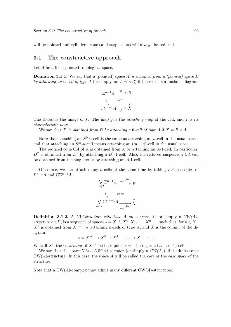
Section 3.1: The constructive approach 96
will be pointed and cylinders, cones and suspensions will always be reduced.
3.1 The constructive approach
Let A be a fixed pointed topological space.
Definition 3.1.1. We say that a (pointed) space X is obtained from a (pointed) space Bby attaching an n-cell of type A (or simply, an A-n-cell) if there exists a pushout diagram
Σn−1Ag //
i
push
B
CΣn−1A f
// X
The A-cell is the image of f . The map g is the attaching map of the cell, and f is itscharacteristic map.
We say that X is obtained from B by attaching a 0-cell of type A if X = B ∨A.
Note that attaching an S0-n-cell is the same as attaching an n-cell in the usual sense,and that attaching an Sm-n-cell means attaching an (m+ n)-cell in the usual sense.
The reduced cone CA of A is obtained from A by attaching an A-1-cell. In particular,D2 is obtained from D1 by attaching a D1-1-cell. Also, the reduced suspension ΣA canbe obtained from the singleton ∗ by attaching an A-1-cell.
Of course, we can attach many n-cells at the same time by taking various copies ofΣn−1A and CΣn−1A. ∨
α∈JΣn−1A
+α∈J
gα
//
i
push
B
∨α∈J
CΣn−1A+
α∈Jfα
// X
Definition 3.1.2. A CW-structure with base A on a space X, or simply a CW(A)-structure on X, is a sequence of spaces ∗ = X−1, X0, X1, . . . , Xn, . . . such that, for n ∈ N0,Xn is obtained from Xn−1 by attaching n-cells of type A, and X is the colimit of the di-agram
∗ = X−1 → X0 → X1 → . . .→ Xn → . . .
We call Xn the n-skeleton of X. The base point ∗ will be regarded as a (−1)-cell.We say that the space X is a CW(A)-complex (or simply a CW(A)), if it admits some
CW(A)-structure. In this case, the space A will be called the core or the base space of thestructure.
Note that a CW(A)-complex may admit many different CW(A)-structures.
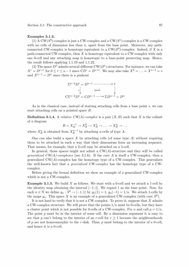
Section 3.1: The constructive approach 97
Examples 3.1.3.(1) A CW(S0)-complex is just a CW-complex and a CW(Sn)-complex is a CW-complex
with no cells of dimension less than n, apart from the base point. Moreover, any path-connected CW-complex is homotopy equivalent to a CW(S0)-complex. Indeed, if X is apath-connected CW-complex, then X is homotopy equivalent to a CW-complex with onlyone 0-cell and any attaching map is homotopic to a base-point preserving map. Hence,the result follows applying 1.1.19 and 1.1.22.
(2) The spaceDn admits several different CW(D1)-structures. For instance, we can takeXr = Dr+1 for 0 ≤ r ≤ n− 1 since CDr = Dr+1. We may also take X0 = . . . = Xn−2 = ∗and Xn−1 = Dn since there is a pushout
Σn−2D1 = Dn−1 //
i
push
∗
CΣn−2D1 = CDn−1 // ΣDn−1 = Dn
As in the classical case, instead of starting attaching cells from a base point ∗, we canstart attaching cells on a pointed space B.
Definition 3.1.4. A relative CW(A)-complex is a pair (X,B) such that X is the colimitof a diagram
B = X−1B → X0
B → X1B → . . .→ Xn
B → . . .
where XnB is obtained from Xn−1
B by attaching n-cells of type A.
One can also build a space X by attaching cells (of some type A) without requiringthem to be attached in such a way that their dimensions form an increasing sequence.That means, for example, that a 2-cell may be attached on a 5-cell.
In general, those spaces might not admit a CW(A)-structure and they will be calledgeneralized CW(A)-complexes (see 3.1.6). If the core A is itself a CW-complex, then ageneralized CW(A)-complex has the homotopy type of a CW-complex. This generalizesthe well-known fact that a generalized CW-complex has the homotopy type of a CW-complex.
Before giving the formal definition we show an example of a generalized CW-complexwhich is not a CW-complex.
Example 3.1.5. We build X as follows. We start with a 0-cell and we attach a 1-cell bythe identity map obtaining the interval [−1; 1]. We regard 1 as the base point. Now, foreach n ∈ N we define gn : S0 → [−1, 1] by gn(1) = 1, gn(−1) = 1/n. We attach 1-cells bythe maps gn. This space X is an example of a generalized CW-complex (with core S0).
It is not hard to verify that it is not a CW-complex. To prove it, suppose that X admitsa CW-complex structure. We will prove that the points 1/n must be 0-cells, but they havea cluster point which is not possible for 0-cells of a CW-complex. Fix n and call p = 1/n.The point p must be in the interior of some cell. By a dimension argument it is easy tosee that p can’t belong to the interior of an r-cell for r ≥ 1 because the neighbourhoodsof p are not homeomorphic to the r-disk. Thus, p must belong to the interior of a 0-cell,and hence it is a 0-cell.
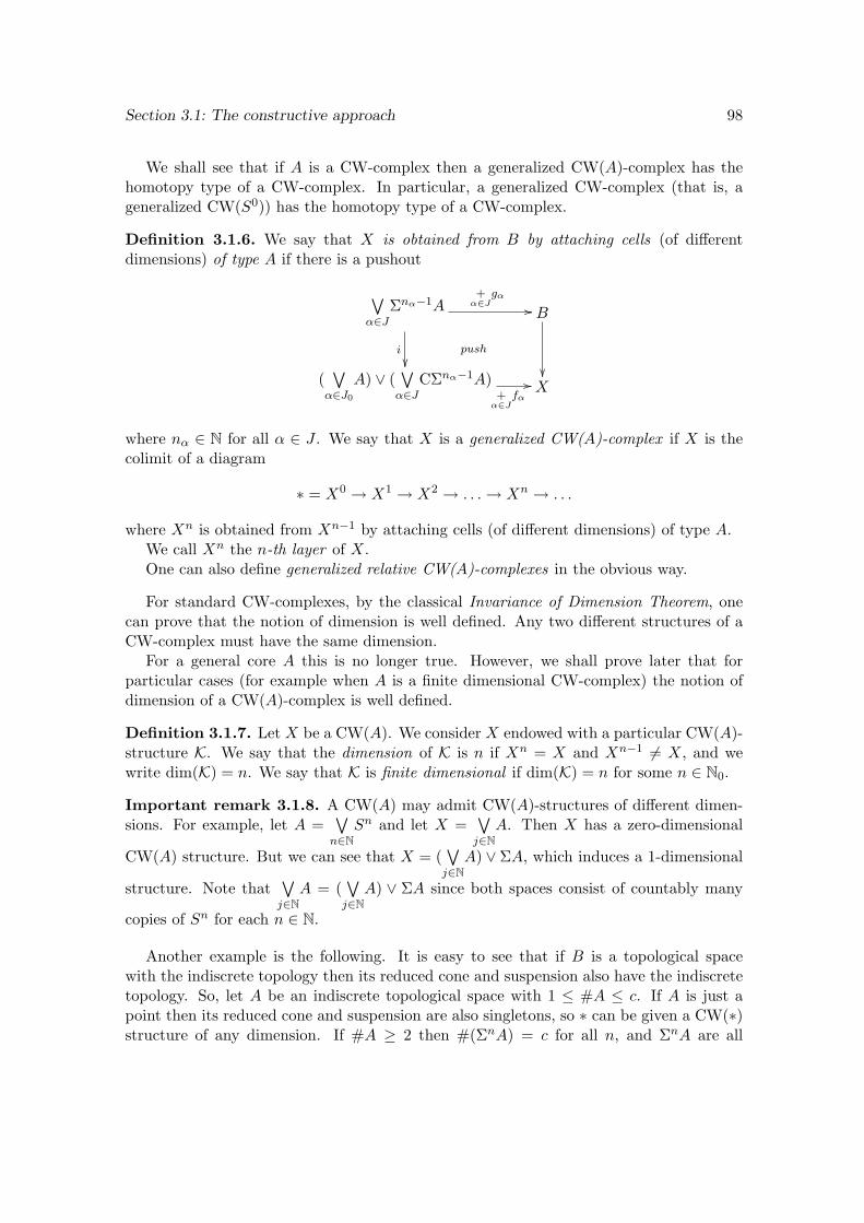
Section 3.1: The constructive approach 98
We shall see that if A is a CW-complex then a generalized CW(A)-complex has thehomotopy type of a CW-complex. In particular, a generalized CW-complex (that is, ageneralized CW(S0)) has the homotopy type of a CW-complex.
Definition 3.1.6. We say that X is obtained from B by attaching cells (of differentdimensions) of type A if there is a pushout
∨α∈J
Σnα−1A+
α∈Jgα
//
i
push
B
(∨α∈J0
A) ∨ (∨α∈J
CΣnα−1A)+
α∈Jfα
// X
where nα ∈ N for all α ∈ J . We say that X is a generalized CW(A)-complex if X is thecolimit of a diagram
∗ = X0 → X1 → X2 → . . .→ Xn → . . .
where Xn is obtained from Xn−1 by attaching cells (of different dimensions) of type A.We call Xn the n-th layer of X.One can also define generalized relative CW(A)-complexes in the obvious way.
For standard CW-complexes, by the classical Invariance of Dimension Theorem, onecan prove that the notion of dimension is well defined. Any two different structures of aCW-complex must have the same dimension.
For a general core A this is no longer true. However, we shall prove later that forparticular cases (for example when A is a finite dimensional CW-complex) the notion ofdimension of a CW(A)-complex is well defined.
Definition 3.1.7. Let X be a CW(A). We consider X endowed with a particular CW(A)-structure K. We say that the dimension of K is n if Xn = X and Xn−1 6= X, and wewrite dim(K) = n. We say that K is finite dimensional if dim(K) = n for some n ∈ N0.
Important remark 3.1.8. A CW(A) may admit CW(A)-structures of different dimen-sions. For example, let A =
∨n∈N
Sn and let X =∨j∈N
A. Then X has a zero-dimensional
CW(A) structure. But we can see that X = (∨j∈N
A) ∨ ΣA, which induces a 1-dimensional
structure. Note that∨j∈N
A = (∨j∈N
A) ∨ ΣA since both spaces consist of countably many
copies of Sn for each n ∈ N.
Another example is the following. It is easy to see that if B is a topological spacewith the indiscrete topology then its reduced cone and suspension also have the indiscretetopology. So, let A be an indiscrete topological space with 1 ≤ #A ≤ c. If A is just apoint then its reduced cone and suspension are also singletons, so ∗ can be given a CW(∗)structure of any dimension. If #A ≥ 2 then #(ΣnA) = c for all n, and ΣnA are all
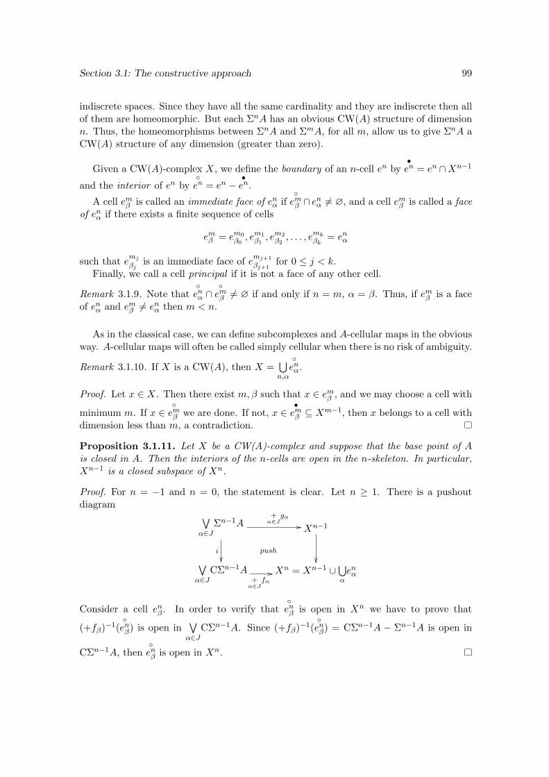
Section 3.1: The constructive approach 99
indiscrete spaces. Since they have all the same cardinality and they are indiscrete then allof them are homeomorphic. But each ΣnA has an obvious CW(A) structure of dimensionn. Thus, the homeomorphisms between ΣnA and ΣmA, for all m, allow us to give ΣnA aCW(A) structure of any dimension (greater than zero).
Given a CW(A)-complex X, we define the boundary of an n-cell en by•en = en ∩Xn−1
and the interior of en byen = en −
•en.
A cell emβ is called an immediate face of enα ifemβ ∩ enα 6= ∅, and a cell emβ is called a face
of enα if there exists a finite sequence of cells
emβ = em0β0, em1β1, em2β2, . . . , emk
βk= enα
such that emj
βjis an immediate face of emj+1
βj+1for 0 ≤ j < k.
Finally, we call a cell principal if it is not a face of any other cell.
Remark 3.1.9. Note thatenα ∩
emβ 6= ∅ if and only if n = m, α = β. Thus, if emβ is a face
of enα and emβ 6= enα then m < n.
As in the classical case, we can define subcomplexes and A-cellular maps in the obviousway. A-cellular maps will often be called simply cellular when there is no risk of ambiguity.
Remark 3.1.10. If X is a CW(A), then X =⋃n,α
enα.
Proof. Let x ∈ X. Then there exist m,β such that x ∈ emβ , and we may choose a cell with
minimum m. If x ∈emβ we are done. If not, x ∈
•emβ ⊆ Xm−1, then x belongs to a cell with
dimension less than m, a contradiction.
Proposition 3.1.11. Let X be a CW(A)-complex and suppose that the base point of Ais closed in A. Then the interiors of the n-cells are open in the n-skeleton. In particular,Xn−1 is a closed subspace of Xn.
Proof. For n = −1 and n = 0, the statement is clear. Let n ≥ 1. There is a pushoutdiagram ∨
α∈JΣn−1A
+α∈J
gα
//
i
push
Xn−1
∨α∈J
CΣn−1A+
α∈Jfα
// Xn = Xn−1 ∪⋃αenα
Consider a cell enβ. In order to verify thatenβ is open in Xn we have to prove that
(+fβ)−1(enβ) is open in
∨α∈J
CΣn−1A. Since (+fβ)−1(enβ) = CΣn−1A − Σn−1A is open in
CΣn−1A, thenenβ is open in Xn.
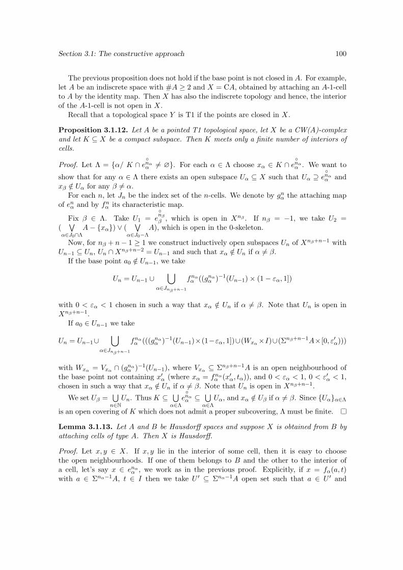
Section 3.1: The constructive approach 100
The previous proposition does not hold if the base point is not closed in A. For example,let A be an indiscrete space with #A ≥ 2 and X = CA, obtained by attaching an A-1-cellto A by the identity map. Then X has also the indiscrete topology and hence, the interiorof the A-1-cell is not open in X.
Recall that a topological space Y is T1 if the points are closed in X.
Proposition 3.1.12. Let A be a pointed T1 topological space, let X be a CW(A)-complexand let K ⊆ X be a compact subspace. Then K meets only a finite number of interiors ofcells.
Proof. Let Λ = α/ K ∩enαα 6= ∅. For each α ∈ Λ choose xα ∈ K ∩
enαα . We want to
show that for any α ∈ Λ there exists an open subspace Uα ⊆ X such that Uα ⊇enαα and
xβ /∈ Uα for any β 6= α.For each n, let Jn be the index set of the n-cells. We denote by gnα the attaching map
of enα and by fnα its characteristic map.
Fix β ∈ Λ. Take U1 =enβ
β , which is open in Xnβ . If nβ = −1, we take U2 =(∨
α∈J0∩Λ
A− xα) ∨ (∨
α∈J0−Λ
A), which is open in the 0-skeleton.
Now, for nβ + n− 1 ≥ 1 we construct inductively open subspaces Un of Xnβ+n−1 withUn−1 ⊆ Un, Un ∩Xnβ+n−2 = Un−1 and such that xα /∈ Un if α 6= β.
If the base point a0 /∈ Un−1, we take
Un = Un−1 ∪⋃
α∈Jnβ+n−1
fnαα ((gnα
α )−1(Un−1)× (1− εα, 1])
with 0 < εα < 1 chosen in such a way that xα /∈ Un if α 6= β. Note that Un is open inXnβ+n−1.
If a0 ∈ Un−1 we take
Un = Un−1∪⋃
α∈Jnβ+n−1
fnαα (((gnα
α )−1(Un−1)×(1−εα, 1])∪(Wxα×I)∪(Σnβ+n−1A× [0, ε′α)))
with Wxα = Vxα ∩ (gnαα )−1(Un−1), where Vxα ⊆ Σnβ+n−1A is an open neighbourhood of
the base point not containing x′α (where xα = fnαα (x′α, tα)), and 0 < εα < 1, 0 < ε′α < 1,
chosen in such a way that xα /∈ Un if α 6= β. Note that Un is open in Xnβ+n−1.
We set Uβ =⋃n∈N
Un. Thus K ⊆⋃α∈Λ
enαα ⊆
⋃α∈Λ
Uα, and xα /∈ Uβ if α 6= β. Since Uαα∈Λ
is an open covering of K which does not admit a proper subcovering, Λ must be finite.
Lemma 3.1.13. Let A and B be Hausdorff spaces and suppose X is obtained from B byattaching cells of type A. Then X is Hausdorff.
Proof. Let x, y ∈ X. If x, y lie in the interior of some cell, then it is easy to choosethe open neighbourhoods. If one of them belongs to B and the other to the interior ofa cell, let’s say x ∈ enα
α , we work as in the previous proof. Explicitly, if x = fα(a, t)with a ∈ Σnα−1A, t ∈ I then we take U ′ ⊆ Σnα−1A open set such that a ∈ U ′ and
Section 3.1: The constructive approach 101
a0 /∈ U ′, where a0 is the basepoint of Σnα−1A. We define U = fα(U ′ × (t/2, (1 + t)/2)),and V = X − fα(U ′ × [t/2, (1 + t)/2]).
If x, y ∈ B, since B is Hausdorff there exist U ′, V ′ ⊆ B open disjoint sets such thatx ∈ U ′ and y ∈ V ′. However, U ′ and V ′ need not be open in X. Suppose first that x, yare both different from the base point. So we may suppose that neither U ′ nor V ′ containthe base point. We take
U = U ′ ∪⋃α∈J
fα((gα)−1(U ′)× (1/2; 1])
V = V ′ ∪⋃α∈J
fα((gα)−1(V ′)× (1/2; 1])
If x is the base point then we take
U = U ′ ∪⋃α∈J
fα(((gα)−1(U ′)× I) ∪ (Σnα−1A× [0; 1/2)))
Proposition 3.1.14. Let A be a Hausdorff space and let X be a CW(A)-complex. ThenX is a Hausdorff space.
Proof. By the previous lemma and induction we have that Xn is a Hausdorff space for alln ≥ −1. Given x, y ∈ X, choose m ∈ N such that x, y ∈ Xm. As Xm is a Hausdorff space,there exist disjoint sets U0 and V0, which are open in Xm, such that x ∈ U0 and y ∈ V0.Proceeding in a similar way as we did in the previous results we construct inductively setsUk, Vk for k ∈ N such that Uk, Vk ⊆ Xm+k are open sets, Uk∩Vk = ∅, Uk∩Xm+k−1 = Uk−1
and Vk ∩Xm+k−1 = Vk−1 for all k ∈ N. We take U =⋃Uk, V =
⋃Vk.
Remark 3.1.15. Let X be a CW(A)-complex and S ⊆ X a subspace. Then S is closed inX if and only if S ∩ enα is closed in enα for all n, α.
Proposition 3.1.16. Let A be a finite dimensional CW-complex, A 6= ∗, and let X be aCW(A). Let K and K′ be CW(A)-structures in X and let n,m ∈ N0 ∪ ∞ denote theirdimensions. Then n = m.
Proof. We suppose first that K and K′ are finite dimensional and n ≥ m.
Let k = dim(A) and let enα be an n-cell of K. There is a homeomorphismenα '
CΣn−1A − Σn−1A, andenα is open in X. Let e be a cell of maximum dimension of the
CW-complex CΣn−1A and let U =e. Thus U is open in X and homeomorphic to
Dn+k.
Now, U intersects some interiors of cells of type A of K′. Let e0 be one of those cellswith maximum dimension. Suppose e0 is an m′-cell, with m′ ≤ m. Then
e0 is open in the
m′-skeleton of X with the K′ structure. It is not hard to see that V = U ∩ e0 is open in U ,extending
e0 to an open subset of X as in the proof of 3.1.12. Indeed, let U0 be an open
subset of X such that U0∩Xm′=e0. Note that U ⊆ Xm′
. Hence, U0∩U ⊆ U0∩Xm′=e0.
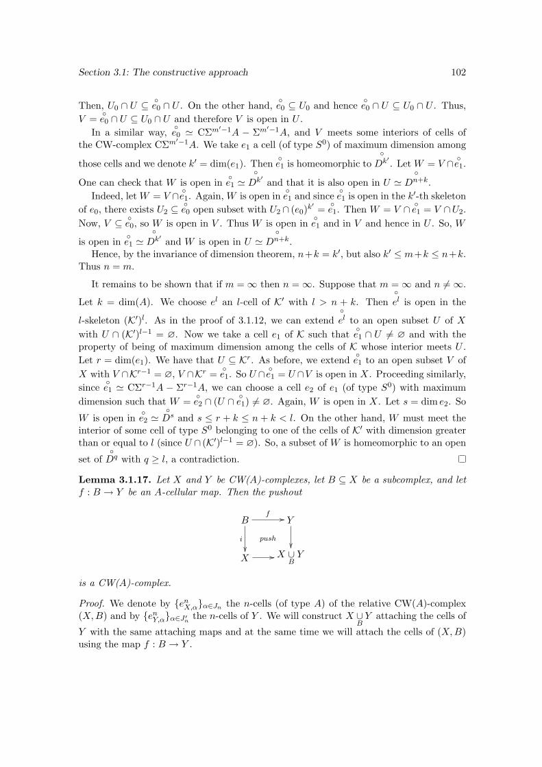
Section 3.1: The constructive approach 102
Then, U0 ∩ U ⊆ e0 ∩ U . On the other hand,
e0 ⊆ U0 and hence
e0 ∩ U ⊆ U0 ∩ U . Thus,
V =e0 ∩ U ⊆ U0 ∩ U and therefore V is open in U .
In a similar way,e0 ' CΣm′−1A − Σm′−1A, and V meets some interiors of cells of
the CW-complex CΣm′−1A. We take e1 a cell (of type S0) of maximum dimension among
those cells and we denote k′ = dim(e1). Thene1 is homeomorphic to
Dk′ . Let W = V ∩ e1.
One can check that W is open ine1 '
Dk′ and that it is also open in U '
Dn+k.
Indeed, let W = V ∩ e1. Again, W is open ine1 and since
e1 is open in the k′-th skeleton
of e0, there exists U2 ⊆e0 open subset with U2 ∩ (e0)k
′=e1. Then W = V ∩ e1 = V ∩U2.
Now, V ⊆ e0, so W is open in V . Thus W is open in
e1 and in V and hence in U . So, W
is open ine1 '
Dk′ and W is open in U '
Dn+k.
Hence, by the invariance of dimension theorem, n+k = k′, but also k′ ≤ m+k ≤ n+k.Thus n = m.
It remains to be shown that if m = ∞ then n = ∞. Suppose that m = ∞ and n 6= ∞.
Let k = dim(A). We choose el an l-cell of K′ with l > n + k. Thenel is open in the
l-skeleton (K′)l. As in the proof of 3.1.12, we can extendel to an open subset U of X
with U ∩ (K′)l−1 = ∅. Now we take a cell e1 of K such thate1 ∩ U 6= ∅ and with the
property of being of maximum dimension among the cells of K whose interior meets U .Let r = dim(e1). We have that U ⊆ Kr. As before, we extend
e1 to an open subset V of
X with V ∩Kr−1 = ∅, V ∩Kr =e1. So U ∩ e1 = U ∩V is open in X. Proceeding similarly,
sincee1 ' CΣr−1A − Σr−1A, we can choose a cell e2 of e1 (of type S0) with maximum
dimension such that W =e2 ∩ (U ∩
e1) 6= ∅. Again, W is open in X. Let s = dim e2. So
W is open ine2 '
Ds and s ≤ r + k ≤ n + k < l. On the other hand, W must meet the
interior of some cell of type S0 belonging to one of the cells of K′ with dimension greaterthan or equal to l (since U ∩ (K′)l−1 = ∅). So, a subset of W is homeomorphic to an open
set ofDq with q ≥ l, a contradiction.
Lemma 3.1.17. Let X and Y be CW(A)-complexes, let B ⊆ X be a subcomplex, and letf : B → Y be an A-cellular map. Then the pushout
Bf //
i
Y
X //
push
X ∪BY
is a CW(A)-complex.
Proof. We denote by enX,αα∈Jn the n-cells (of type A) of the relative CW(A)-complex(X,B) and by enY,αα∈J ′n the n-cells of Y . We will construct X ∪
BY attaching the cells of
Y with the same attaching maps and at the same time we will attach the cells of (X,B)using the map f : B → Y .
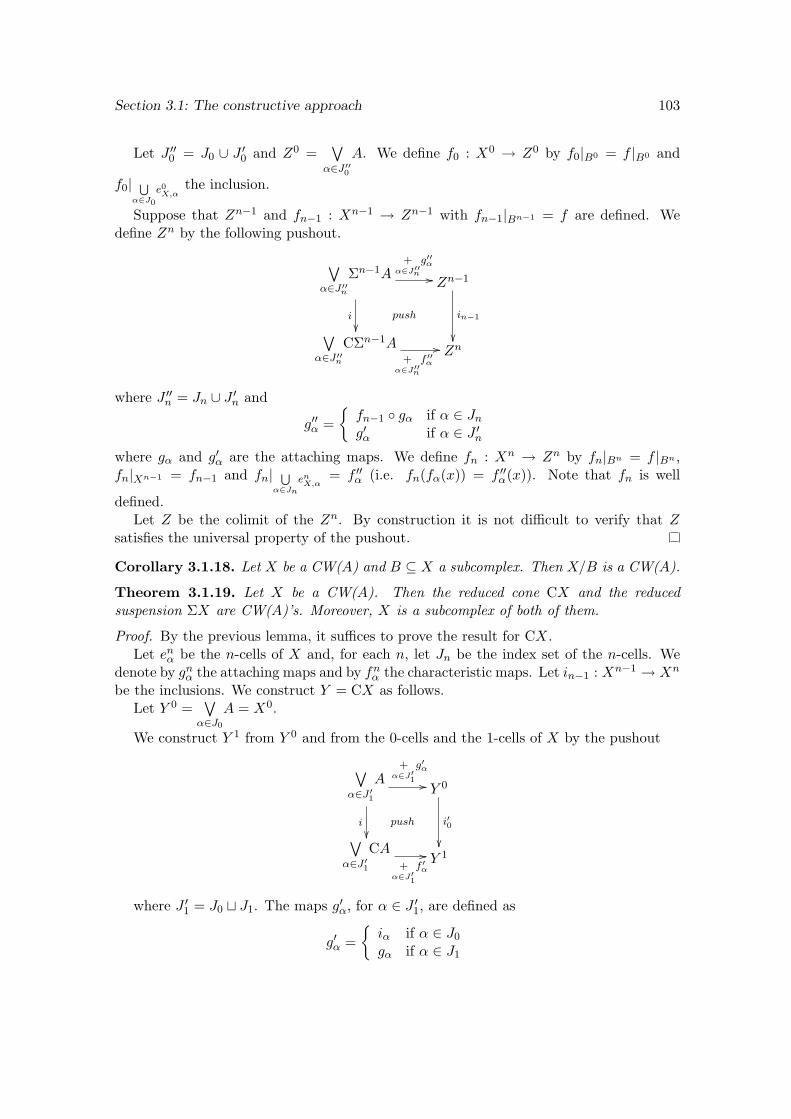
Section 3.1: The constructive approach 103
Let J ′′0 = J0 ∪ J ′0 and Z0 =∨
α∈J ′′0A. We define f0 : X0 → Z0 by f0|B0 = f |B0 and
f0| Sα∈J0
e0X,αthe inclusion.
Suppose that Zn−1 and fn−1 : Xn−1 → Zn−1 with fn−1|Bn−1 = f are defined. Wedefine Zn by the following pushout.
∨α∈J ′′n
Σn−1A+
α∈J′′ng′′α
//
i
push
Zn−1
in−1
∨α∈J ′′n
CΣn−1A+
α∈J′′nf ′′α
// Zn
where J ′′n = Jn ∪ J ′n and
g′′α =fn−1 gα if α ∈ Jng′α if α ∈ J ′n
where gα and g′α are the attaching maps. We define fn : Xn → Zn by fn|Bn = f |Bn ,fn|Xn−1 = fn−1 and fn| S
α∈Jn
enX,α
= f ′′α (i.e. fn(fα(x)) = f ′′α(x)). Note that fn is well
defined.Let Z be the colimit of the Zn. By construction it is not difficult to verify that Z
satisfies the universal property of the pushout.
Corollary 3.1.18. Let X be a CW(A) and B ⊆ X a subcomplex. Then X/B is a CW(A).
Theorem 3.1.19. Let X be a CW(A). Then the reduced cone CX and the reducedsuspension ΣX are CW(A)’s. Moreover, X is a subcomplex of both of them.
Proof. By the previous lemma, it suffices to prove the result for CX.Let enα be the n-cells of X and, for each n, let Jn be the index set of the n-cells. We
denote by gnα the attaching maps and by fnα the characteristic maps. Let in−1 : Xn−1 → Xn
be the inclusions. We construct Y = CX as follows.Let Y 0 =
∨α∈J0
A = X0.
We construct Y 1 from Y 0 and from the 0-cells and the 1-cells of X by the pushout
∨α∈J ′1
A+
α∈J′1
g′α
//
i
push
Y 0
i′0
∨α∈J ′1
CA+
α∈J′1
f ′α
// Y 1
where J ′1 = J0 t J1. The maps g′α, for α ∈ J ′1, are defined as
g′α =iα if α ∈ J0
gα if α ∈ J1
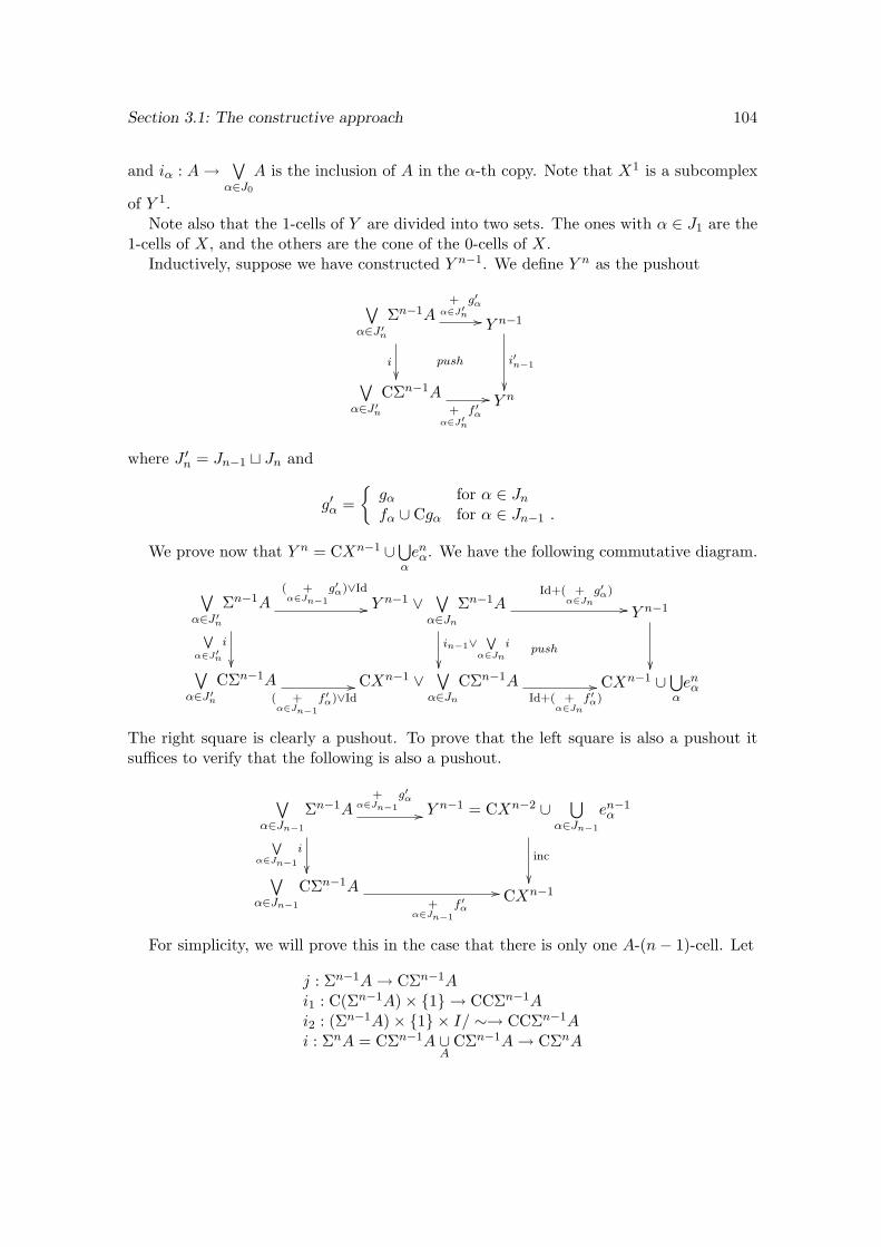
Section 3.1: The constructive approach 104
and iα : A→∨α∈J0
A is the inclusion of A in the α-th copy. Note that X1 is a subcomplex
of Y 1.Note also that the 1-cells of Y are divided into two sets. The ones with α ∈ J1 are the
1-cells of X, and the others are the cone of the 0-cells of X.Inductively, suppose we have constructed Y n−1. We define Y n as the pushout
∨α∈J ′n
Σn−1A+
α∈J′ng′α
//
i
push
Y n−1
i′n−1
∨α∈J ′n
CΣn−1A+
α∈J′nf ′α
// Y n
where J ′n = Jn−1 t Jn and
g′α =gα for α ∈ Jnfα ∪ Cgα for α ∈ Jn−1 .
We prove now that Y n = CXn−1 ∪⋃αenα. We have the following commutative diagram.
∨α∈J ′n
Σn−1A( +α∈Jn−1
g′α)∨Id
//
Wα∈J′n
i
Y n−1 ∨∨
α∈Jn
Σn−1A
in−1∨W
α∈Jn
i
Id+( +α∈Jn
g′α)
//
push
Y n−1
∨α∈J ′n
CΣn−1A( +α∈Jn−1
f ′α)∨Id// CXn−1 ∨
∨α∈Jn
CΣn−1AId+( +
α∈Jnf ′α)// CXn−1 ∪
⋃αenα
The right square is clearly a pushout. To prove that the left square is also a pushout itsuffices to verify that the following is also a pushout.
∨α∈Jn−1
Σn−1A+
α∈Jn−1
g′α
//
Wα∈Jn−1
i
Y n−1 = CXn−2 ∪⋃
α∈Jn−1
en−1α
inc
∨α∈Jn−1
CΣn−1A+
α∈Jn−1
f ′α
// CXn−1
For simplicity, we will prove this in the case that there is only one A-(n− 1)-cell. Let
j : Σn−1A→ CΣn−1Ai1 : C(Σn−1A)× 1 → CCΣn−1Ai2 : (Σn−1A)× 1 × I/ ∼→ CCΣn−1Ai : ΣnA = CΣn−1A ∪
ACΣn−1A→ CΣnA
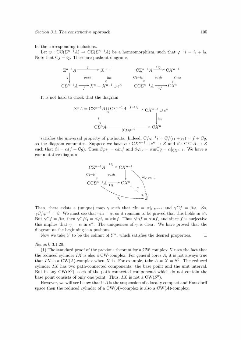
Section 3.1: The constructive approach 105
be the corresponding inclusions.Let ϕ : CC(Σn−1A) → CΣ(Σn−1A) be a homeomorphism, such that ϕ−1i = i1 + i2.
Note that Cj = i2. There are pushout diagrams
Σn−1Ag //
j
push
Xn−1
inc
CΣn−1A f// Xn = Xn−1 ∪ en
CΣn−1ACg //
Cj=i2
push
CXn−1
Cinc
CCΣn−1A Cf
// CXn
It is not hard to check that the diagram
ΣnA = CΣn−1A ∪A
CΣn−1A f+Cg //
i
CXn−1 ∪ en
inc
CΣnA
(Cf)ϕ−1// CXn
satisfies the universal property of pushouts. Indeed, Cfϕ−1i = Cf(i1 + i2) = f + Cg,so the diagram commutes. Suppose we have α : CXn−1 ∪ en → Z and β : CΣnA → Zsuch that βi = α(f + Cg). Then βϕi1 = αinf and βϕi2 = αinCg = α|CXn−1 . We have acommutative diagram
CΣn−1ACg //
Cj=i2
push
CXn−1
α|CXn−1
CCΣn−1A Cf//
βϕ 00
CXn
γ
##Z
Then, there exists a (unique) map γ such that γin = α|CXn−1 and γCf = βϕ. So,γCfϕ−1 = β. We must see that γin = α, so it remains to be proved that this holds in en.But γCf = βϕ, then γCfi1 = βϕi1 = αinf . Thus γinf = αinf , and since f is surjectivethis implies that γ = α in en. The uniqueness of γ is clear. We have proved that thediagram at the beginning is a pushout.
Now we take Y to be the colimit of Y n, which satisfies the desired properties.
Remark 3.1.20.(1) The standard proof of the previous theorem for a CW-complex X uses the fact that
the reduced cylinder IX is also a CW-complex. For general cores A, it is not always truethat IX is a CW(A)-complex when X is. For example, take A = X = S0. The reducedcylinder IX has two path-connected components: the base point and the unit interval.But in any CW(S0), each of the path connected components which do not contain thebase point consists of only one point. Thus, IX is not a CW(S0).
However, we will see below that if A is the suspension of a locally compact and Hausdorffspace then the reduced cylinder of a CW(A)-complex is also a CW(A)-complex.
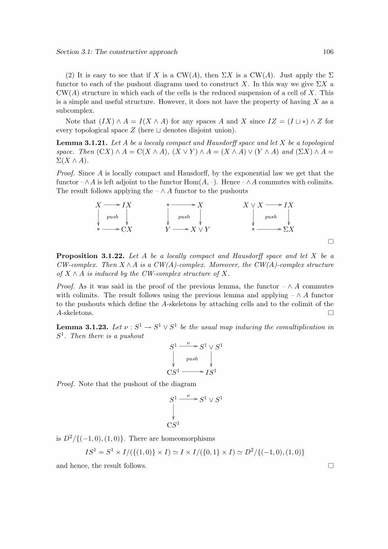
Section 3.1: The constructive approach 106
(2) It is easy to see that if X is a CW(A), then ΣX is a CW(A). Just apply the Σfunctor to each of the pushout diagrams used to construct X. In this way we give ΣX aCW(A) structure in which each of the cells is the reduced suspension of a cell of X. Thisis a simple and useful structure. However, it does not have the property of having X as asubcomplex.
Note that (IX) ∧ A = I(X ∧ A) for any spaces A and X since IZ = (I t ∗) ∧ Z forevery topological space Z (here t denotes disjoint union).
Lemma 3.1.21. Let A be a loccaly compact and Hausdorff space and let X be a topologicalspace. Then (CX) ∧ A = C(X ∧ A), (X ∨ Y ) ∧ A = (X ∧ A) ∨ (Y ∧ A) and (ΣX) ∧ A =Σ(X ∧A).
Proof. Since A is locally compact and Hausdorff, by the exponential law we get that thefunctor –∧A is left adjoint to the functor Hom(A, –). Hence –∧A commutes with colimits.The result follows applying the – ∧A functor to the pushouts
X //
push
IX
∗ // CX
∗ //
push
X
Y // X ∨ Y
X ∨X //
push
IX
∗ // ΣX
Proposition 3.1.22. Let A be a locally compact and Hausdorff space and let X be aCW-complex. Then X ∧A is a CW(A)-complex. Moreover, the CW(A)-complex structureof X ∧A is induced by the CW-complex structure of X.
Proof. As it was said in the proof of the previous lemma, the functor – ∧ A commuteswith colimits. The result follows using the previous lemma and applying – ∧ A functorto the pushouts which define the A-skeletons by attaching cells and to the colimit of theA-skeletons.
Lemma 3.1.23. Let ν : S1 → S1 ∨ S1 be the usual map inducing the comultiplication inS1. Then there is a pushout
S1 ν //
push
S1 ∨ S1
CS1 // IS1
Proof. Note that the pushout of the diagram
S1 ν //
S1 ∨ S1
CS1
is D2/(−1, 0), (1, 0). There are homeomorphisms
IS1 = S1 × I/((1, 0) × I) ' I × I/(0, 1 × I) ' D2/(−1, 0), (1, 0)
and hence, the result follows.
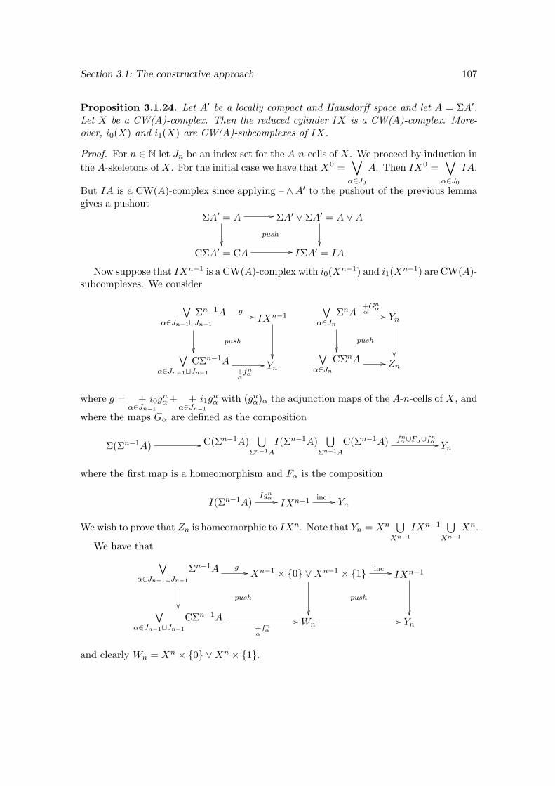
Section 3.1: The constructive approach 107
Proposition 3.1.24. Let A′ be a locally compact and Hausdorff space and let A = ΣA′.Let X be a CW(A)-complex. Then the reduced cylinder IX is a CW(A)-complex. More-over, i0(X) and i1(X) are CW(A)-subcomplexes of IX.
Proof. For n ∈ N let Jn be an index set for the A-n-cells of X. We proceed by induction inthe A-skeletons of X. For the initial case we have that X0 =
∨α∈J0
A. Then IX0 =∨α∈J0
IA.
But IA is a CW(A)-complex since applying – ∧A′ to the pushout of the previous lemmagives a pushout
ΣA′ = A //
push
ΣA′ ∨ ΣA′ = A ∨A
CΣA′ = CA // IΣA′ = IA
Now suppose that IXn−1 is a CW(A)-complex with i0(Xn−1) and i1(Xn−1) are CW(A)-subcomplexes. We consider
∨α∈Jn−1tJn−1
Σn−1A g //
push
IXn−1
∨α∈Jn−1tJn−1
CΣn−1A+αfn
α
// Yn
∨α∈Jn
ΣnA+αGn
α
//
push
Yn
∨α∈Jn
CΣnA // Zn
where g = +α∈Jn−1
i0gnα+ +
α∈Jn−1
i1gnα with (gnα)α the adjunction maps of the A-n-cells of X, and
where the maps Gα are defined as the composition
Σ(Σn−1A) // C(Σn−1A)⋃
Σn−1A
I(Σn−1A)⋃
Σn−1A
C(Σn−1A) fnα∪Fα∪fn
α // Yn
where the first map is a homeomorphism and Fα is the composition
I(Σn−1A)Ign
α // IXn−1 inc // Yn
We wish to prove that Zn is homeomorphic to IXn. Note that Yn = Xn⋃
Xn−1
IXn−1⋃
Xn−1
Xn.
We have that ∨α∈Jn−1tJn−1
Σn−1A g //
push
Xn−1 × 0 ∨Xn−1 × 1 inc //
push
IXn−1
∨α∈Jn−1tJn−1
CΣn−1A+αfn
α
//Wn// Yn
and clearly Wn = Xn × 0 ∨Xn × 1.
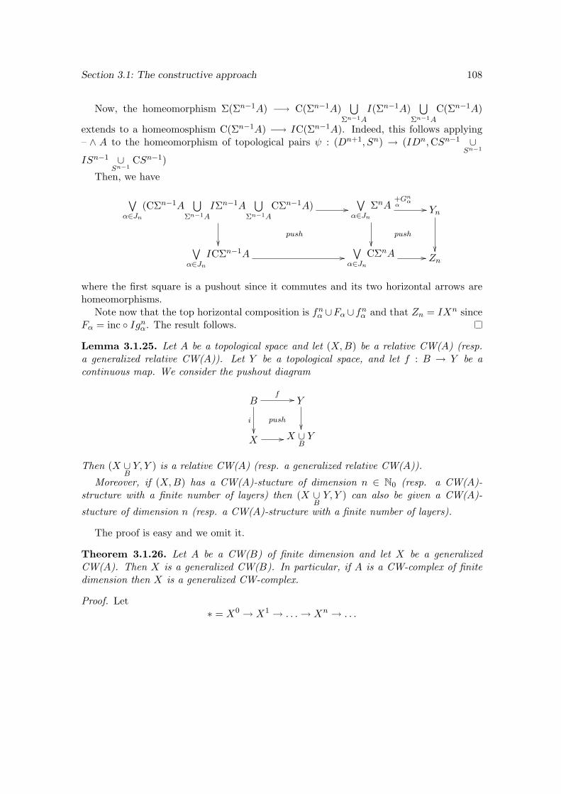
Section 3.1: The constructive approach 108
Now, the homeomorphism Σ(Σn−1A) −→ C(Σn−1A)⋃
Σn−1A
I(Σn−1A)⋃
Σn−1A
C(Σn−1A)
extends to a homeomosphism C(Σn−1A) −→ IC(Σn−1A). Indeed, this follows applying– ∧ A to the homeomorphism of topological pairs ψ : (Dn+1, Sn) → (IDn,CSn−1 ∪
Sn−1
ISn−1 ∪Sn−1
CSn−1)
Then, we have
∨α∈Jn
(CΣn−1A⋃
Σn−1A
IΣn−1A⋃
Σn−1A
CΣn−1A) //
push
∨α∈Jn
ΣnA+αGn
α
//
push
Yn
∨α∈Jn
ICΣn−1A //∨
α∈Jn
CΣnA // Zn
where the first square is a pushout since it commutes and its two horizontal arrows arehomeomorphisms.
Note now that the top horizontal composition is fnα ∪Fα∪fnα and that Zn = IXn sinceFα = inc Ignα. The result follows.
Lemma 3.1.25. Let A be a topological space and let (X,B) be a relative CW(A) (resp.a generalized relative CW(A)). Let Y be a topological space, and let f : B → Y be acontinuous map. We consider the pushout diagram
Bf //
i
Y
X //
push
X ∪BY
Then (X ∪BY, Y ) is a relative CW(A) (resp. a generalized relative CW(A)).
Moreover, if (X,B) has a CW(A)-stucture of dimension n ∈ N0 (resp. a CW(A)-structure with a finite number of layers) then (X ∪
BY, Y ) can also be given a CW(A)-
stucture of dimension n (resp. a CW(A)-structure with a finite number of layers).
The proof is easy and we omit it.
Theorem 3.1.26. Let A be a CW(B) of finite dimension and let X be a generalizedCW(A). Then X is a generalized CW(B). In particular, if A is a CW-complex of finitedimension then X is a generalized CW-complex.
Proof. Let∗ = X0 → X1 → . . .→ Xn → . . .
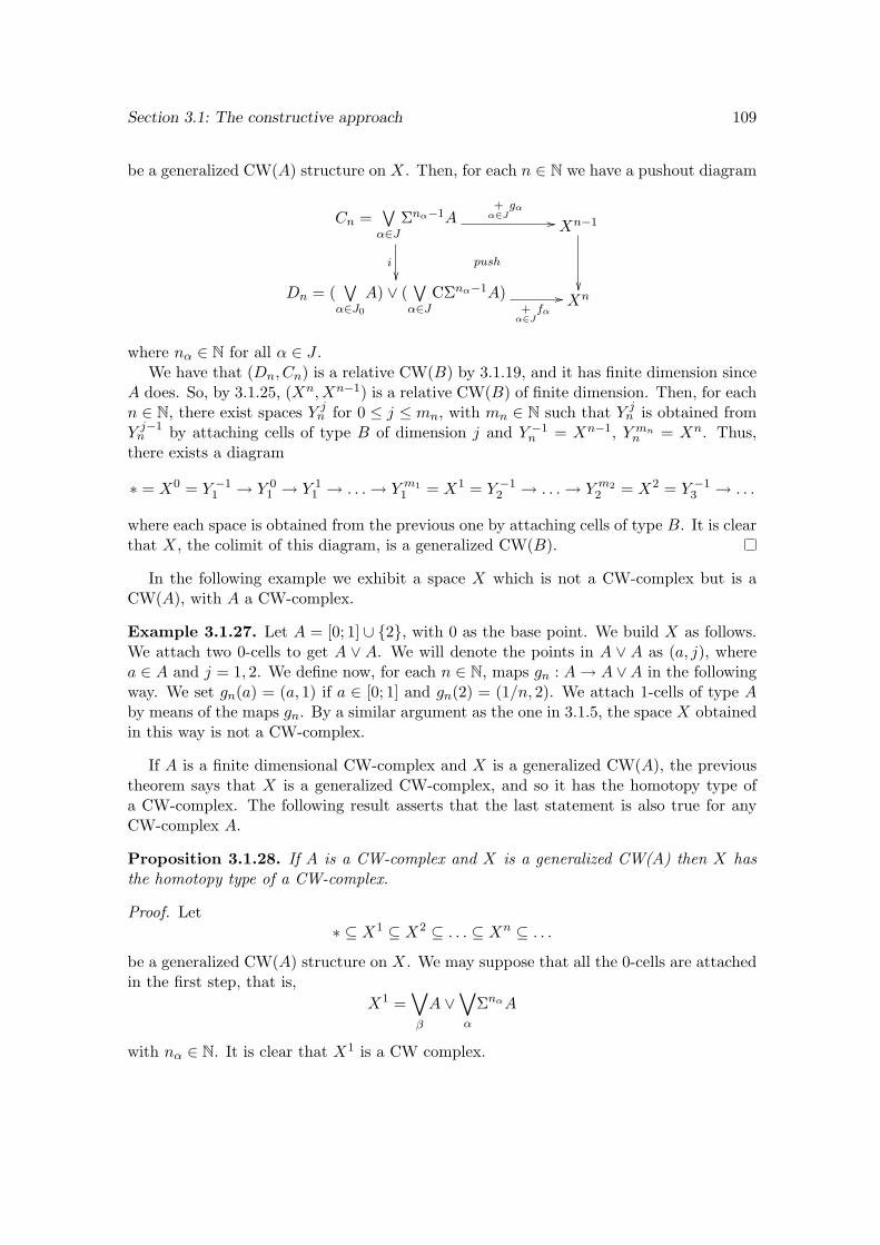
Section 3.1: The constructive approach 109
be a generalized CW(A) structure on X. Then, for each n ∈ N we have a pushout diagram
Cn =∨α∈J
Σnα−1A+
α∈Jgα
//
i
push
Xn−1
Dn = (∨α∈J0
A) ∨ (∨α∈J
CΣnα−1A)+
α∈Jfα
// Xn
where nα ∈ N for all α ∈ J .We have that (Dn, Cn) is a relative CW(B) by 3.1.19, and it has finite dimension since
A does. So, by 3.1.25, (Xn, Xn−1) is a relative CW(B) of finite dimension. Then, for eachn ∈ N, there exist spaces Y j
n for 0 ≤ j ≤ mn, with mn ∈ N such that Y jn is obtained from
Y j−1n by attaching cells of type B of dimension j and Y −1
n = Xn−1, Y mnn = Xn. Thus,
there exists a diagram
∗ = X0 = Y −11 → Y 0
1 → Y 11 → . . .→ Y m1
1 = X1 = Y −12 → . . .→ Y m2
2 = X2 = Y −13 → . . .
where each space is obtained from the previous one by attaching cells of type B. It is clearthat X, the colimit of this diagram, is a generalized CW(B).
In the following example we exhibit a space X which is not a CW-complex but is aCW(A), with A a CW-complex.
Example 3.1.27. Let A = [0; 1] ∪ 2, with 0 as the base point. We build X as follows.We attach two 0-cells to get A ∨ A. We will denote the points in A ∨ A as (a, j), wherea ∈ A and j = 1, 2. We define now, for each n ∈ N, maps gn : A→ A ∨A in the followingway. We set gn(a) = (a, 1) if a ∈ [0; 1] and gn(2) = (1/n, 2). We attach 1-cells of type Aby means of the maps gn. By a similar argument as the one in 3.1.5, the space X obtainedin this way is not a CW-complex.
If A is a finite dimensional CW-complex and X is a generalized CW(A), the previoustheorem says that X is a generalized CW-complex, and so it has the homotopy type ofa CW-complex. The following result asserts that the last statement is also true for anyCW-complex A.
Proposition 3.1.28. If A is a CW-complex and X is a generalized CW(A) then X hasthe homotopy type of a CW-complex.
Proof. Let∗ ⊆ X1 ⊆ X2 ⊆ . . . ⊆ Xn ⊆ . . .
be a generalized CW(A) structure on X. We may suppose that all the 0-cells are attachedin the first step, that is,
X1 =∨β
A ∨∨α
ΣnαA
with nα ∈ N. It is clear that X1 is a CW complex.
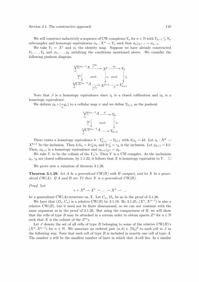
Section 3.1: The constructive approach 110
We will construct inductively a sequence of CW-complexes Yn for n ∈ N with Yn−1 ⊆ Ynsubcomplex and homotopy equivalences φn : Xn → Yn such that φn|Xn−1 = φn−1.
We take Y1 = X1 and φ1 the identity map. Suppose we have already constructedY1, . . . , Yk and φ1, . . . , φk satisfying the conditions mentioned above. We consider thefollowing pushout diagram.
∨αΣnα−1A
+αgα
//
Wαi
push
Xk
ik
φk //
push
Yk
γ′k
∨αCΣnα−1A
+αfα
// Xk+1β// Y ′k+1
Note that β is a homotopy equivalence since ik is a closed cofibration and φk is ahomotopy equivalence.
We deform φk (+αgα) to a cellular map ψ and we define Yk+1 as the pushout∨
αΣnα−1A ψ //
Wαi
push
Yk
γk
∨αCΣnα−1A // Yk+1
There exists a homotopy equivalence k : Y ′k+1 → Yk+1 with k|Yk= Id. Let ik : Xk →
Xk+1 be the inclusion. Then kβik = kγ′kφk and kγ′k = γk is the inclusion. Let φk+1 = kβ.Then, φk+1 is a homotopy equivalence and φk+1|Xk = φk.
We take Y to be the colimit of the Yn’s. Then Y is a CW-complex. As the inclusionsik, γk are closed cofibrations, by 1.1.22, it follows that X is homotopy equivalent to Y .
We prove now a variation of theorem 3.1.26.
Theorem 3.1.29. Let A be a generalized CW(B) with B compact, and let X be a gener-alized CW(A). If A and B are T1 then X is a generalized CW(B).
Proof. Let∗ = X0 → X1 → . . .→ Xn → . . .
be a generalized CW(A)-structure on X. Let Cn, Dn be as in the proof of 3.1.26.We have that (Dn, Cn) is a relative CW(B) by 3.1.19. By 3.1.25, (Xn, Xn−1) is also a
relative CW(B), but it need not be finite dimensional, so we can not continue with thesame argument as in the proof of 3.1.26. But using the compactness of B, we will showthat the cells of type B may be attached in a certain order to obtain spaces Zn for n ∈ Nsuch that X is the colimit of the Zn’s.
Let J denote the set of all cells of type B belonging to some of the relative CW(B)’s(Xn, Xn−1) for n ∈ N. We associate an ordered pair (a, b) ∈ (N0)2 to each cell in J inthe following way. Note that each cell of type B is included in exactly one cell of type A.The number a will be the smallest number of layer in which that A-cell lies. In a similar
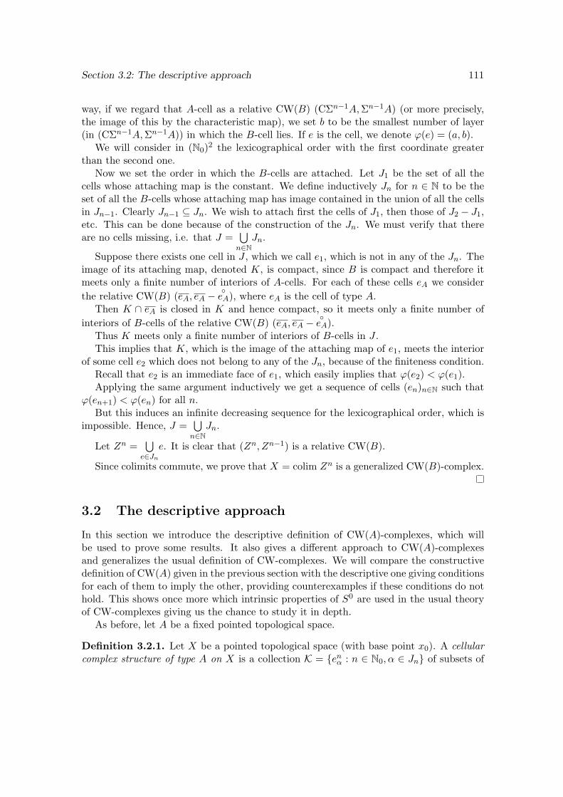
Section 3.2: The descriptive approach 111
way, if we regard that A-cell as a relative CW(B) (CΣn−1A,Σn−1A) (or more precisely,the image of this by the characteristic map), we set b to be the smallest number of layer(in (CΣn−1A,Σn−1A)) in which the B-cell lies. If e is the cell, we denote ϕ(e) = (a, b).
We will consider in (N0)2 the lexicographical order with the first coordinate greaterthan the second one.
Now we set the order in which the B-cells are attached. Let J1 be the set of all thecells whose attaching map is the constant. We define inductively Jn for n ∈ N to be theset of all the B-cells whose attaching map has image contained in the union of all the cellsin Jn−1. Clearly Jn−1 ⊆ Jn. We wish to attach first the cells of J1, then those of J2 − J1,etc. This can be done because of the construction of the Jn. We must verify that thereare no cells missing, i.e. that J =
⋃n∈N
Jn.
Suppose there exists one cell in J , which we call e1, which is not in any of the Jn. Theimage of its attaching map, denoted K, is compact, since B is compact and therefore itmeets only a finite number of interiors of A-cells. For each of these cells eA we considerthe relative CW(B) (eA, eA −
eA), where eA is the cell of type A.
Then K ∩ eA is closed in K and hence compact, so it meets only a finite number ofinteriors of B-cells of the relative CW(B) (eA, eA −
eA).
Thus K meets only a finite number of interiors of B-cells in J .This implies that K, which is the image of the attaching map of e1, meets the interior
of some cell e2 which does not belong to any of the Jn, because of the finiteness condition.Recall that e2 is an immediate face of e1, which easily implies that ϕ(e2) < ϕ(e1).Applying the same argument inductively we get a sequence of cells (en)n∈N such that
ϕ(en+1) < ϕ(en) for all n.But this induces an infinite decreasing sequence for the lexicographical order, which is
impossible. Hence, J =⋃n∈N
Jn.
Let Zn =⋃e∈Jn
e. It is clear that (Zn, Zn−1) is a relative CW(B).
Since colimits commute, we prove that X = colim Zn is a generalized CW(B)-complex.
3.2 The descriptive approach
In this section we introduce the descriptive definition of CW(A)-complexes, which willbe used to prove some results. It also gives a different approach to CW(A)-complexesand generalizes the usual definition of CW-complexes. We will compare the constructivedefinition of CW(A) given in the previous section with the descriptive one giving conditionsfor each of them to imply the other, providing counterexamples if these conditions do nothold. This shows once more which intrinsic properties of S0 are used in the usual theoryof CW-complexes giving us the chance to study it in depth.
As before, let A be a fixed pointed topological space.
Definition 3.2.1. Let X be a pointed topological space (with base point x0). A cellularcomplex structure of type A on X is a collection K = enα : n ∈ N0, α ∈ Jn of subsets of
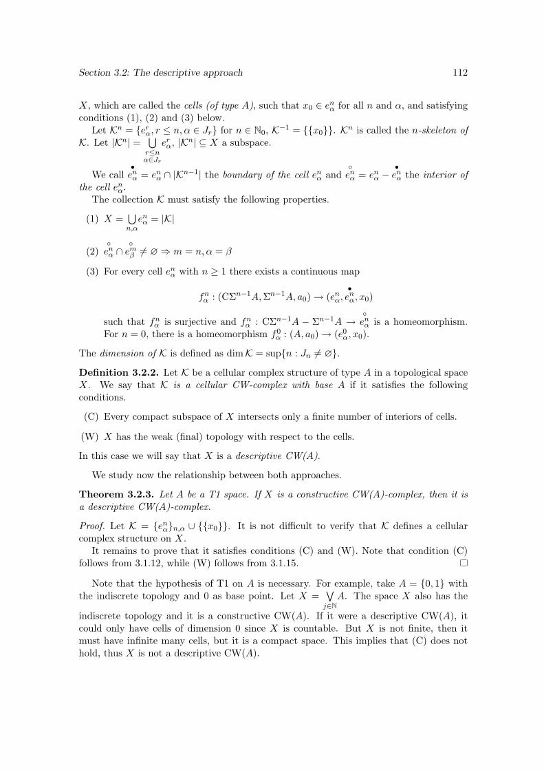
Section 3.2: The descriptive approach 112
X, which are called the cells (of type A), such that x0 ∈ enα for all n and α, and satisfyingconditions (1), (2) and (3) below.
Let Kn = erα, r ≤ n, α ∈ Jr for n ∈ N0, K−1 = x0. Kn is called the n-skeleton ofK. Let |Kn| =
⋃r≤nα∈Jr
erα, |Kn| ⊆ X a subspace.
We call•enα = enα ∩ |Kn−1| the boundary of the cell enα and
enα = enα −
•enα the interior of
the cell enα.The collection K must satisfy the following properties.
(1) X =⋃n,αenα = |K|
(2)enα ∩
emβ 6= ∅ ⇒ m = n, α = β
(3) For every cell enα with n ≥ 1 there exists a continuous map
fnα : (CΣn−1A,Σn−1A, a0) → (enα,•enα, x0)
such that fnα is surjective and fnα : CΣn−1A − Σn−1A →enα is a homeomorphism.
For n = 0, there is a homeomorphism f0α : (A, a0) → (e0α, x0).
The dimension of K is defined as dimK = supn : Jn 6= ∅.
Definition 3.2.2. Let K be a cellular complex structure of type A in a topological spaceX. We say that K is a cellular CW-complex with base A if it satisfies the followingconditions.
(C) Every compact subspace of X intersects only a finite number of interiors of cells.
(W) X has the weak (final) topology with respect to the cells.
In this case we will say that X is a descriptive CW(A).
We study now the relationship between both approaches.
Theorem 3.2.3. Let A be a T1 space. If X is a constructive CW(A)-complex, then it isa descriptive CW(A)-complex.
Proof. Let K = enαn,α ∪ x0. It is not difficult to verify that K defines a cellularcomplex structure on X.
It remains to prove that it satisfies conditions (C) and (W). Note that condition (C)follows from 3.1.12, while (W) follows from 3.1.15.
Note that the hypothesis of T1 on A is necessary. For example, take A = 0, 1 withthe indiscrete topology and 0 as base point. Let X =
∨j∈N
A. The space X also has the
indiscrete topology and it is a constructive CW(A). If it were a descriptive CW(A), itcould only have cells of dimension 0 since X is countable. But X is not finite, then itmust have infinite many cells, but it is a compact space. This implies that (C) does nothold, thus X is not a descriptive CW(A).
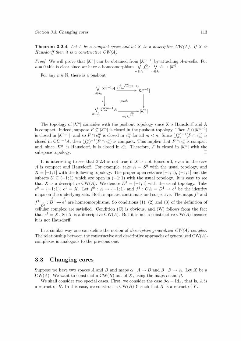
Section 3.3: Changing cores 113
Theorem 3.2.4. Let A be a compact space and let X be a descriptive CW(A). If X isHausdorff then it is a constructive CW(A).
Proof. We will prove that |Kn| can be obtained from |Kn−1| by attaching A-n-cells. Forn = 0 this is clear since we have a homeomorphism
∨α∈J0
f0α :
∨α∈J0
A→ |K0|.
For any n ∈ N, there is a pushout
∨α∈Jn
Σn−1A+
α∈Jnfn
α |Σn−1A
//
i
push
|Kn−1|
∨α∈Jn
CΣn−1A+
α∈Jnfn
α
// |Kn|
The topology of |Kn| coincides with the pushout topology since X is Hausdorff and Ais compact. Indeed, suppose F ⊆ |Kn| is closed in the pushout topology. Then F ∩ |Kn−1|is closed in |Kn−1|, and so F ∩ emβ is closed in emβ for all m < n. Since (fnα )−1(F ∩ enα) isclosed in CΣn−1A, then (fnα )−1(F ∩ enα) is compact. This implies that F ∩ enα is compactand, since |Kn| is Hausdorff, it is closed in enα. Therefore, F is closed in |Kn| with thesubspace topology.
It is interesting to see that 3.2.4 is not true if X is not Hausdorff, even in the caseA is compact and Hausdorff. For example, take A = S0 with the usual topology, andX = [−1; 1] with the following topology. The proper open sets are [−1; 1), (−1; 1] and thesubsets U ⊆ (−1; 1) which are open in (−1; 1) with the usual topology. It is easy to seethat X is a descriptive CW(A). We denote D1 = [−1; 1] with the usual topology. Takee0 = −1; 1, e1 = X. Let f0 : A → −1; 1 and f1 : CA = D1 → e1 be the identitymaps on the underlying sets. Both maps are continuous and surjective. The maps f0 and
f1| D1
:D1 →
e1 are homeomorphisms. So conditions (1), (2) and (3) of the definition of
cellular complex are satisfied. Condition (C) is obvious, and (W) follows from the factthat e1 = X. So X is a descriptive CW(A). But it is not a constructive CW(A) becauseit is not Hausdorff.
In a similar way one can define the notion of descriptive generalized CW(A)-complex.The relationship between the constructive and descriptive approachs of generalized CW(A)-complexes is analogous to the previous one.
3.3 Changing cores
Suppose we have two spaces A and B and maps α : A → B and β : B → A. Let X be aCW(A). We want to construct a CW(B) out of X, using the maps α and β.
We shall consider two special cases. First, we consider the case βα = IdA, that is, A isa retract of B. In this case, we construct a CW(B) Y such that X is a retract of Y .
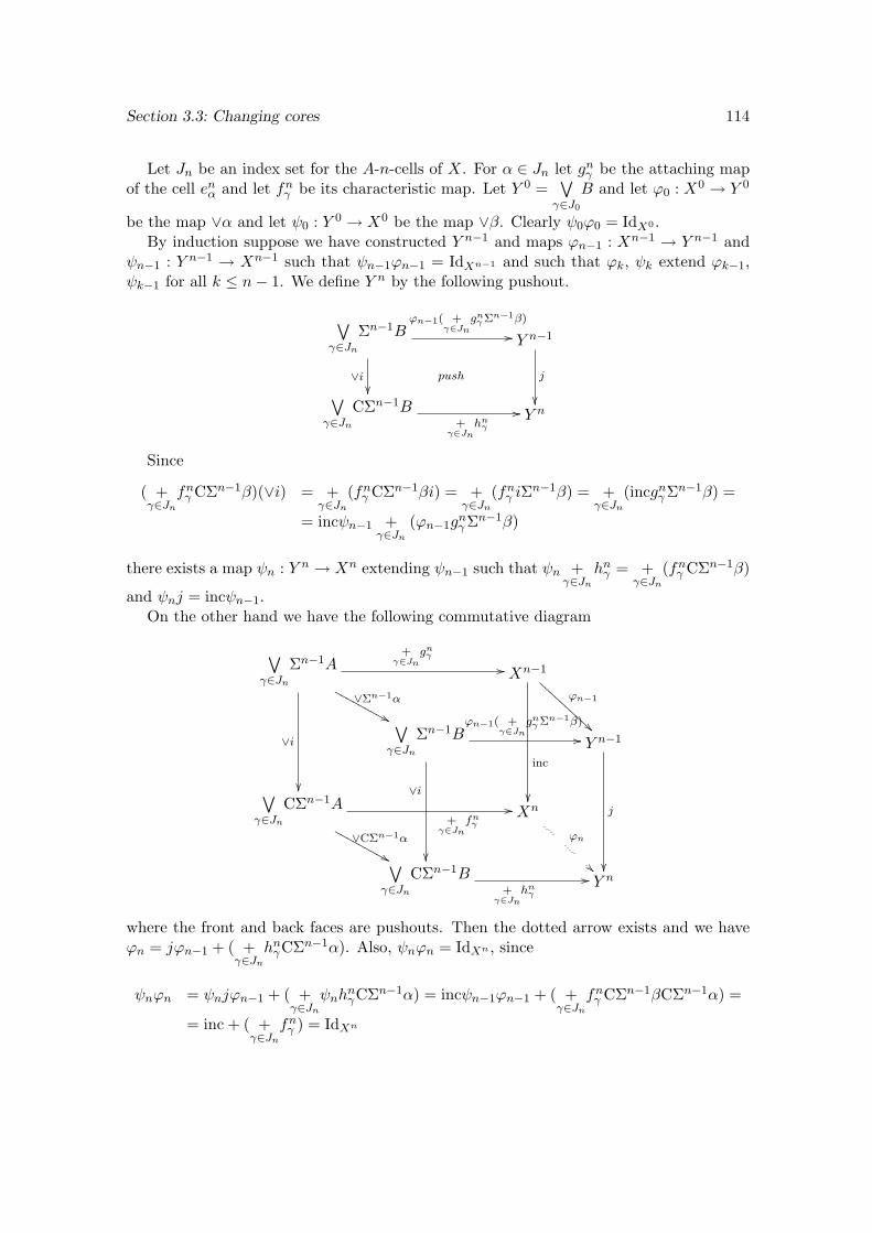
Section 3.3: Changing cores 114
Let Jn be an index set for the A-n-cells of X. For α ∈ Jn let gnγ be the attaching mapof the cell enα and let fnγ be its characteristic map. Let Y 0 =
∨γ∈J0
B and let ϕ0 : X0 → Y 0
be the map ∨α and let ψ0 : Y 0 → X0 be the map ∨β. Clearly ψ0ϕ0 = IdX0 .By induction suppose we have constructed Y n−1 and maps ϕn−1 : Xn−1 → Y n−1 and
ψn−1 : Y n−1 → Xn−1 such that ψn−1ϕn−1 = IdXn−1 and such that ϕk, ψk extend ϕk−1,ψk−1 for all k ≤ n− 1. We define Y n by the following pushout.
∨γ∈Jn
Σn−1Bϕn−1( +
γ∈Jngn
γ Σn−1β)
//
∨i
push
Y n−1
j
∨γ∈Jn
CΣn−1B+
γ∈Jnhn
γ
// Y n
Since
( +γ∈Jn
fnγ CΣn−1β)(∨i) = +γ∈Jn
(fnγ CΣn−1βi) = +γ∈Jn
(fnγ iΣn−1β) = +
γ∈Jn
(incgnγΣn−1β) =
= incψn−1 +γ∈Jn
(ϕn−1gnγΣn−1β)
there exists a map ψn : Y n → Xn extending ψn−1 such that ψn +γ∈Jn
hnγ = +γ∈Jn
(fnγ CΣn−1β)
and ψnj = incψn−1.On the other hand we have the following commutative diagram
∨γ∈Jn
Σn−1A+
γ∈Jngn
γ
//
∨i
∨Σn−1α
&&MMMMMMMMMXn−1
inc
ϕn−1
BBB
BBBB
BBB
∨γ∈Jn
Σn−1Bϕn−1( +
γ∈Jngn
γ Σn−1β)
//
∨i
Y n−1
j
∨γ∈Jn
CΣn−1A+
γ∈Jnfn
γ
//
∨CΣn−1α
&&MMMMMMMMMXn
ϕn
∨γ∈Jn
CΣn−1B+
γ∈Jnhn
γ
// Y n
where the front and back faces are pushouts. Then the dotted arrow exists and we haveϕn = jϕn−1 + ( +
γ∈Jn
hnγCΣn−1α). Also, ψnϕn = IdXn , since
ψnϕn = ψnjϕn−1 + ( +γ∈Jn
ψnhnγCΣn−1α) = incψn−1ϕn−1 + ( +
γ∈Jn
fnγ CΣn−1βCΣn−1α) =
= inc + ( +γ∈Jn
fnγ ) = IdXn
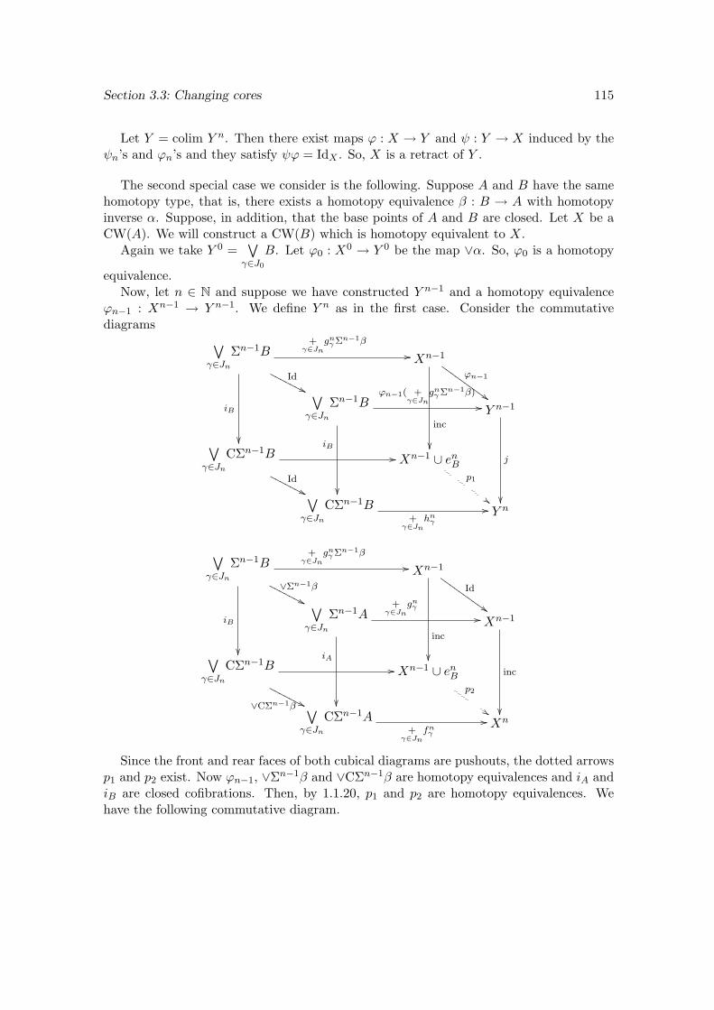
Section 3.3: Changing cores 115
Let Y = colim Y n. Then there exist maps ϕ : X → Y and ψ : Y → X induced by theψn’s and ϕn’s and they satisfy ψϕ = IdX . So, X is a retract of Y .
The second special case we consider is the following. Suppose A and B have the samehomotopy type, that is, there exists a homotopy equivalence β : B → A with homotopyinverse α. Suppose, in addition, that the base points of A and B are closed. Let X be aCW(A). We will construct a CW(B) which is homotopy equivalent to X.
Again we take Y 0 =∨γ∈J0
B. Let ϕ0 : X0 → Y 0 be the map ∨α. So, ϕ0 is a homotopy
equivalence.Now, let n ∈ N and suppose we have constructed Y n−1 and a homotopy equivalence
ϕn−1 : Xn−1 → Y n−1. We define Y n as in the first case. Consider the commutativediagrams ∨
γ∈Jn
Σn−1B+
γ∈Jngn
γ Σn−1β
//
iB
Id
''NNNNNNNXn−1
inc
ϕn−1
##HHHHHHHHHH
∨γ∈Jn
Σn−1Bϕn−1( +
γ∈Jngn
γ Σn−1β)
//
iB
Y n−1
j
∨γ∈Jn
CΣn−1B //
Id
''NNNNNNNXn−1 ∪ enB
p1
##∨γ∈Jn
CΣn−1B+
γ∈Jnhn
γ
// Y n
∨γ∈Jn
Σn−1B+
γ∈Jngn
γ Σn−1β
//
iB
∨Σn−1β
''NNNNNNNXn−1
inc
Id
$$HHHHHHHHHH
∨γ∈Jn
Σn−1A+
γ∈Jngn
γ
//
iA
Xn−1
inc
∨γ∈Jn
CΣn−1B //
∨CΣn−1β ''NNNNNNN
Xn−1 ∪ enBp2
$$∨γ∈Jn
CΣn−1A+
γ∈Jnfn
γ
// Xn
Since the front and rear faces of both cubical diagrams are pushouts, the dotted arrowsp1 and p2 exist. Now ϕn−1, ∨Σn−1β and ∨CΣn−1β are homotopy equivalences and iA andiB are closed cofibrations. Then, by 1.1.20, p1 and p2 are homotopy equivalences. Wehave the following commutative diagram.
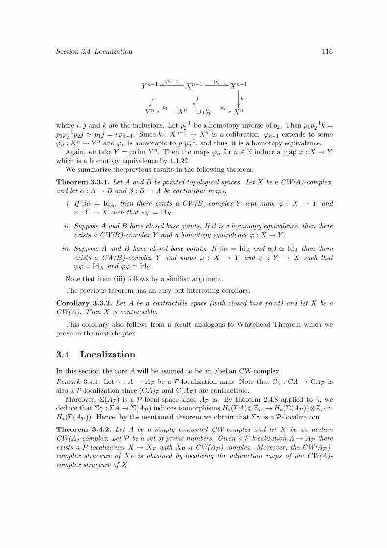
Section 3.4: Localization 116
Y n−1
i
Xn−1ϕn−1oo Id //
j
Xn−1
k
Y n Xn−1 ∪ enB
p1oo p2 // Xn
where i, j and k are the inclusions. Let p−12 be a homotopy inverse of p2. Then p1p
−12 k =
p1p−12 p2j ' p1j = iϕn−1. Since k : Xn−1 → Xn is a cofibration, ϕn−1 extends to some
ϕn : Xn → Y n and ϕn is homotopic to p1p−12 , and thus, it is a homotopy equivalence.
Again, we take Y = colim Y n. Then the maps ϕn for n ∈ N induce a map ϕ : X → Ywhich is a homotopy equivalence by 1.1.22.
We summarize the previous results in the following theorem.
Theorem 3.3.1. Let A and B be pointed topological spaces. Let X be a CW(A)-complex,and let α : A→ B and β : B → A be continuous maps.
i. If βα = IdA, then there exists a CW(B)-complex Y and maps ϕ : X → Y andψ : Y → X such that ψϕ = IdX .
ii. Suppose A and B have closed base points. If β is a homotopy equivalence, then thereexists a CW(B)-complex Y and a homotopy equivalence ϕ : X → Y .
iii. Suppose A and B have closed base points. If βα = IdA and αβ ' IdA then thereexists a CW(B)-complex Y and maps ϕ : X → Y and ψ : Y → X such thatψϕ = IdX and ϕψ ' IdY .
Note that item (iii) follows by a similiar argument.
The previous theorem has an easy but interesting corollary.
Corollary 3.3.2. Let A be a contractible space (with closed base point) and let X be aCW(A). Then X is contractible.
This corollary also follows from a result analogous to Whitehead Theorem which weprove in the next chapter.
3.4 Localization
In this section the core A will be asumed to be an abelian CW-complex.Remark 3.4.1. Let γ : A → AP be a P-localization map. Note that Cγ : CA → CAP isalso a P-localization since (CA)P and C(AP) are contractible.
Moreover, Σ(AP) is a P-local space since AP is. By theorem 2.4.8 applied to γ, wededuce that Σγ : ΣA→ Σ(AP) induces isomorphisms H∗(ΣA)⊗ZP → H∗(Σ(AP))⊗ZP 'H∗(Σ(AP)). Hence, by the mentioned theorem we obtain that Σγ is a P-localization.
Theorem 3.4.2. Let A be a simply connected CW-complex and let X be an abelianCW(A)-complex. Let P be a set of prime numbers. Given a P-localization A→ AP thereexists a P-localization X → XP with XP a CW(AP)-complex. Moreover, the CW(AP)-complex structure of XP is obtained by localizing the adjunction maps of the CW(A)-complex structure of X.
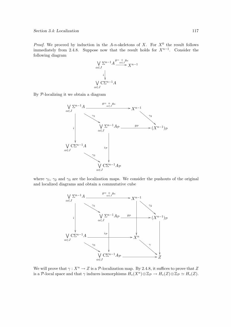
Section 3.4: Localization 117
Proof. We proceed by induction in the A-n-skeletons of X. For X0 the result followsimmediately from 2.4.8. Suppose now that the result holds for Xn−1. Consider thefollowing diagram ∨
α∈JΣn−1A
g= +α∈J
gα
//
i
Xn−1
∨α∈J
CΣn−1A
By P-localizing it we obtain a diagram
∨α∈J
Σn−1Ag= +
α∈Jgα
//
i
γ1
&&LLLLLLLLLLXn−1
γ2
""DDD
DDDD
DDDD
∨α∈J
Σn−1AP gP //
iP
(Xn−1)P
∨α∈J
CΣn−1A
γ3
&&LLLLLLLLLL
∨α∈J
CΣn−1AP
where γ1, γ2 and γ3 are the localization maps. We consider the pushouts of the originaland localized diagrams and obtain a commutative cube
∨α∈J
Σn−1Ag= +
α∈Jgα
//
i
γ1
&&LLLLLLLLLLXn−1
γ2
""DDD
DDDD
DDDD
∨α∈J
Σn−1AP gP //
iP
(Xn−1)P
∨α∈J
CΣn−1A
γ3
&&LLLLLLLLLL
// Xn
γ
""DDDDDDDDDDDD
∨α∈J
CΣn−1AP // Z
We will prove that γ : Xn → Z is a P-localization map. By 2.4.8, it suffices to prove that Zis a P-local space and that γ induces isomorphisms H∗(Xn)⊗ZP → H∗(Z)⊗ZP ' H∗(Z).
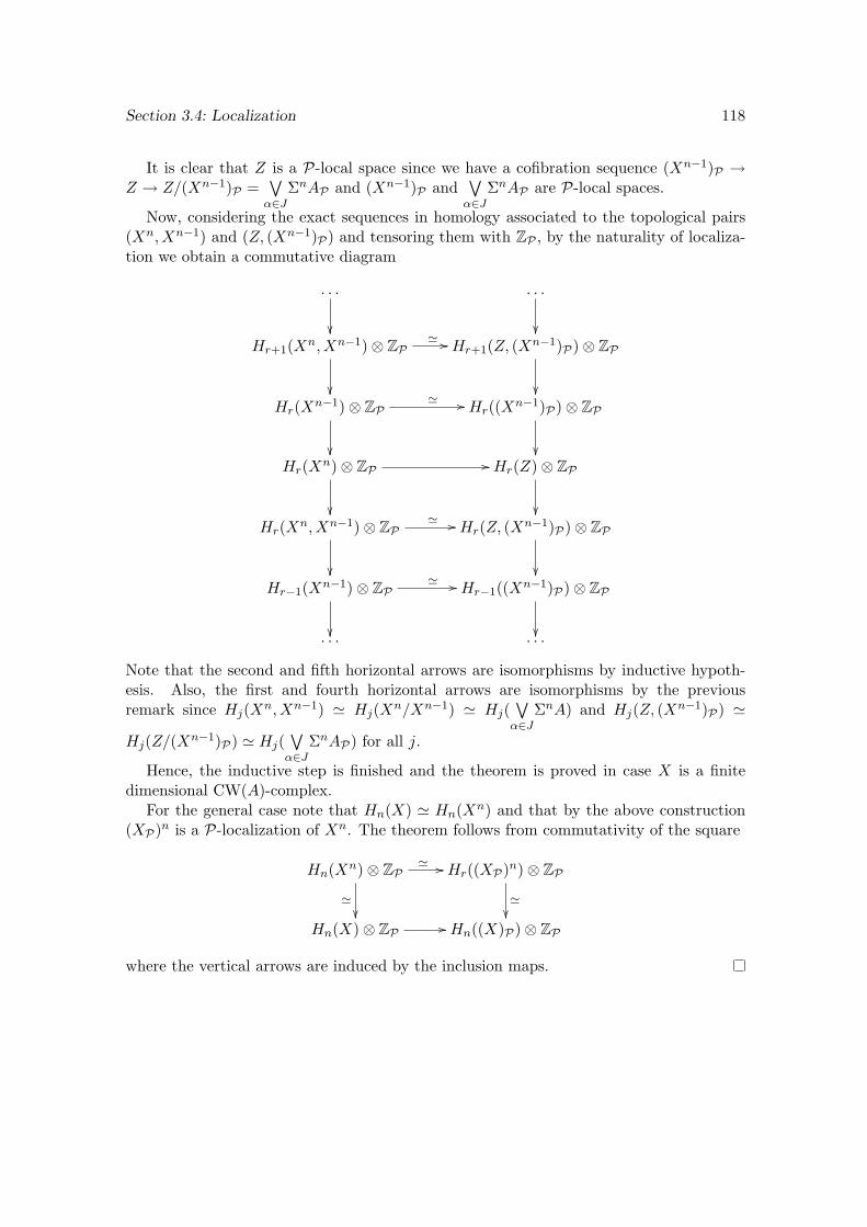
Section 3.4: Localization 118
It is clear that Z is a P-local space since we have a cofibration sequence (Xn−1)P →Z → Z/(Xn−1)P =
∨α∈J
ΣnAP and (Xn−1)P and∨α∈J
ΣnAP are P-local spaces.
Now, considering the exact sequences in homology associated to the topological pairs(Xn, Xn−1) and (Z, (Xn−1)P) and tensoring them with ZP , by the naturality of localiza-tion we obtain a commutative diagram
. . .
. . .
Hr+1(Xn, Xn−1)⊗ ZP
' // Hr+1(Z, (Xn−1)P)⊗ ZP
Hr(Xn−1)⊗ ZP
' // Hr((Xn−1)P)⊗ ZP
Hr(Xn)⊗ ZP
// Hr(Z)⊗ ZP
Hr(Xn, Xn−1)⊗ ZP
' // Hr(Z, (Xn−1)P)⊗ ZP
Hr−1(Xn−1)⊗ ZP
' // Hr−1((Xn−1)P)⊗ ZP
. . . . . .
Note that the second and fifth horizontal arrows are isomorphisms by inductive hypoth-esis. Also, the first and fourth horizontal arrows are isomorphisms by the previousremark since Hj(Xn, Xn−1) ' Hj(Xn/Xn−1) ' Hj(
∨α∈J
ΣnA) and Hj(Z, (Xn−1)P) '
Hj(Z/(Xn−1)P) ' Hj(∨α∈J
ΣnAP) for all j.
Hence, the inductive step is finished and the theorem is proved in case X is a finitedimensional CW(A)-complex.
For the general case note that Hn(X) ' Hn(Xn) and that by the above construction(XP)n is a P-localization of Xn. The theorem follows from commutativity of the square
Hn(Xn)⊗ ZP'
' // Hr((XP)n)⊗ ZP'
Hn(X)⊗ ZP // Hn((X)P)⊗ ZP
where the vertical arrows are induced by the inclusion maps.
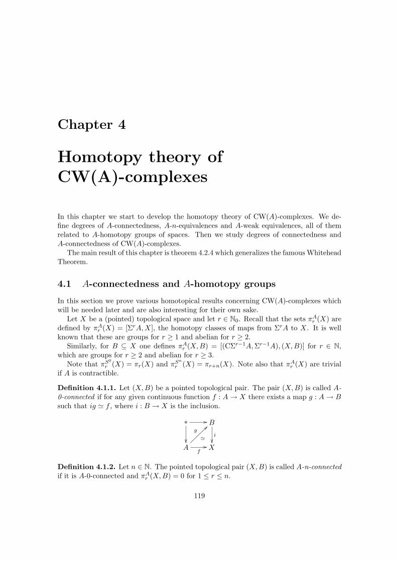
Chapter 4
Homotopy theory ofCW(A)-complexes
In this chapter we start to develop the homotopy theory of CW(A)-complexes. We de-fine degrees of A-connectedness, A-n-equivalences and A-weak equivalences, all of themrelated to A-homotopy groups of spaces. Then we study degrees of connectedness andA-connectedness of CW(A)-complexes.
The main result of this chapter is theorem 4.2.4 which generalizes the famous WhiteheadTheorem.
4.1 A-connectedness and A-homotopy groups
In this section we prove various homotopical results concerning CW(A)-complexes whichwill be needed later and are also interesting for their own sake.
Let X be a (pointed) topological space and let r ∈ N0. Recall that the sets πAr (X) aredefined by πAr (X) = [ΣrA,X], the homotopy classes of maps from ΣrA to X. It is wellknown that these are groups for r ≥ 1 and abelian for r ≥ 2.
Similarly, for B ⊆ X one defines πAr (X,B) = [(CΣr−1A,Σr−1A), (X,B)] for r ∈ N,which are groups for r ≥ 2 and abelian for r ≥ 3.
Note that πS0
r (X) = πr(X) and πSn
r (X) = πr+n(X). Note also that πAr (X) are trivialif A is contractible.
Definition 4.1.1. Let (X,B) be a pointed topological pair. The pair (X,B) is called A-0-connected if for any given continuous function f : A→ X there exists a map g : A→ Bsuch that ig ' f , where i : B → X is the inclusion.
∗ //
'
B
i
Af//
g>>~~~~~~~X
Definition 4.1.2. Let n ∈ N. The pointed topological pair (X,B) is called A-n-connectedif it is A-0-connected and πAr (X,B) = 0 for 1 ≤ r ≤ n.
119
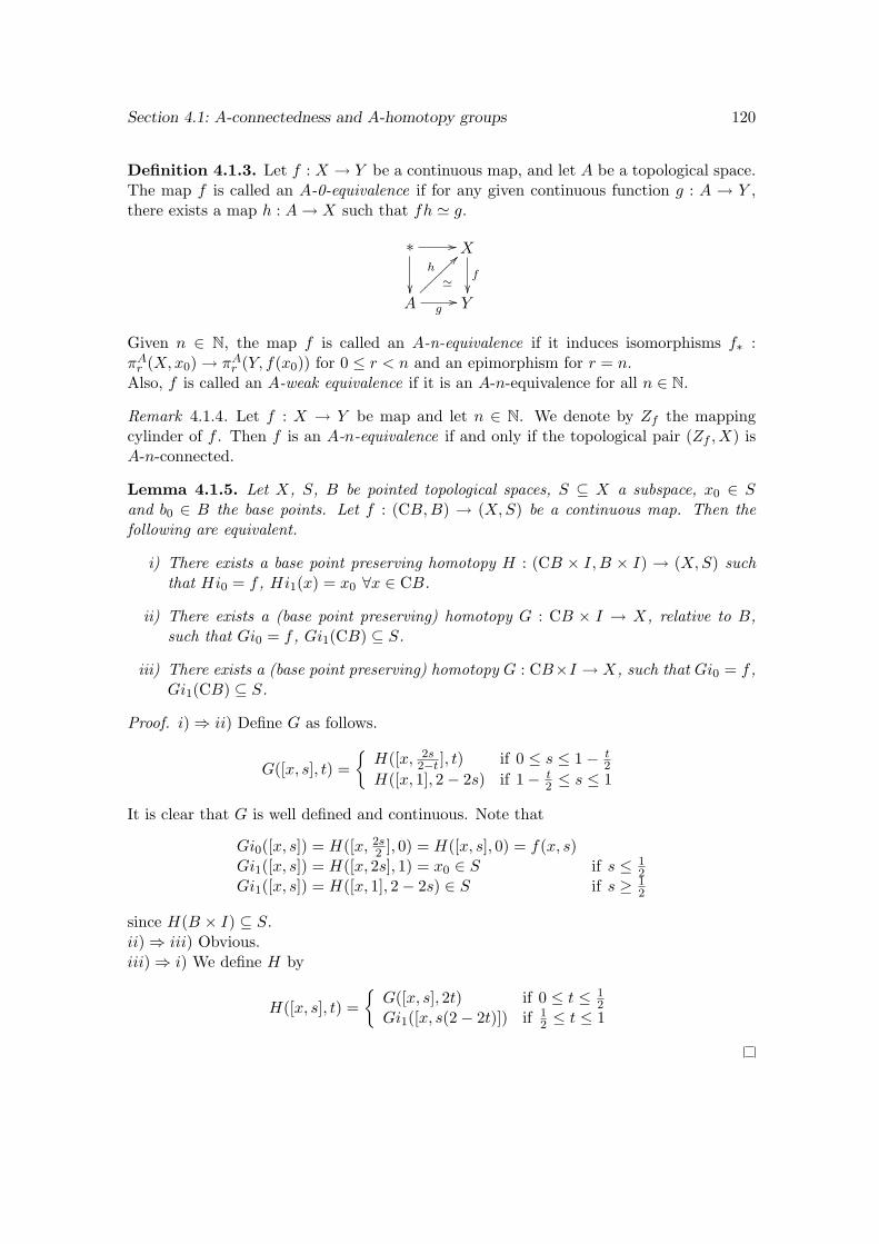
Section 4.1: A-connectedness and A-homotopy groups 120
Definition 4.1.3. Let f : X → Y be a continuous map, and let A be a topological space.The map f is called an A-0-equivalence if for any given continuous function g : A → Y ,there exists a map h : A→ X such that fh ' g.
∗ //
'
X
f
A g//
h>>~~~~~~~Y
Given n ∈ N, the map f is called an A-n-equivalence if it induces isomorphisms f∗ :πAr (X,x0) → πAr (Y, f(x0)) for 0 ≤ r < n and an epimorphism for r = n.Also, f is called an A-weak equivalence if it is an A-n-equivalence for all n ∈ N.
Remark 4.1.4. Let f : X → Y be map and let n ∈ N. We denote by Zf the mappingcylinder of f . Then f is an A-n-equivalence if and only if the topological pair (Zf , X) isA-n-connected.
Lemma 4.1.5. Let X, S, B be pointed topological spaces, S ⊆ X a subspace, x0 ∈ Sand b0 ∈ B the base points. Let f : (CB,B) → (X,S) be a continuous map. Then thefollowing are equivalent.
i) There exists a base point preserving homotopy H : (CB × I,B × I) → (X,S) suchthat Hi0 = f , Hi1(x) = x0 ∀x ∈ CB.
ii) There exists a (base point preserving) homotopy G : CB × I → X, relative to B,such that Gi0 = f , Gi1(CB) ⊆ S.
iii) There exists a (base point preserving) homotopy G : CB×I → X, such that Gi0 = f ,Gi1(CB) ⊆ S.
Proof. i) ⇒ ii) Define G as follows.
G([x, s], t) =H([x, 2s
2−t ], t) if 0 ≤ s ≤ 1− t2
H([x, 1], 2− 2s) if 1− t2 ≤ s ≤ 1
It is clear that G is well defined and continuous. Note that
Gi0([x, s]) = H([x, 2s2 ], 0) = H([x, s], 0) = f(x, s)
Gi1([x, s]) = H([x, 2s], 1) = x0 ∈ S if s ≤ 12
Gi1([x, s]) = H([x, 1], 2− 2s) ∈ S if s ≥ 12
since H(B × I) ⊆ S.ii) ⇒ iii) Obvious.iii) ⇒ i) We define H by
H([x, s], t) =G([x, s], 2t) if 0 ≤ t ≤ 1
2Gi1([x, s(2− 2t)]) if 1
2 ≤ t ≤ 1
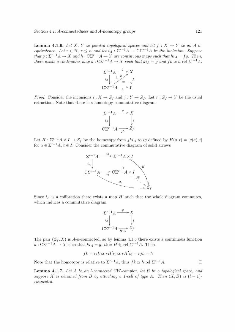
Section 4.1: A-connectedness and A-homotopy groups 121
Lemma 4.1.6. Let X, Y be pointed topological spaces and let f : X → Y be an A-n-equivalence. Let r ∈ N, r ≤ n and let iA : Σr−1A → CΣr−1A be the inclusion. Supposethat g : Σr−1A→ X and h : CΣr−1A→ Y are continuous maps such that hiA = fg. Then,there exists a continuous map k : CΣr−1A→ X such that kiA = g and fk ' h rel Σr−1A.
Σr−1Ag //
iA '|‖
X
f
CΣr−1A h
//
k::vvvvvvvvvY
Proof. Consider the inclusions i : X → Zf and j : Y → Zf . Let r : Zf → Y be the usualretraction. Note that there is a homotopy commutative diagram
Σr−1Ag //
iA
X
i
CΣr−1A jh// Zf
Let H : Σr−1A × I → Zf be the homotopy from jhiA to ig defined by H(a, t) = [g(a), t]for a ∈ Σr−1A, t ∈ I. Consider the commutative diagram of solid arrows
Σr−1Ai0 //
iA
Σr−1A× I
H
CΣr−1A i0//
jh
00
CΣr−1A× IH′
%%Zf
Since iA is a cofibration there exists a map H ′ such that the whole diagram commutes,which induces a commutative diagram
Σr−1Ag //
iA
X
i
CΣr−1AH′i1
// Zf
The pair (Zf , X) is A-n-connected, so by lemma 4.1.5 there exists a continuous functionk : CΣr−1A→ X such that kiA = g, ik ' H ′i1 rel Σr−1A. Then
fk = rik ' rH ′i1 ' rH ′i0 = rjh = h
Note that the homotopy is relative to Σr−1A, thus fk ' h rel Σr−1A.
Lemma 4.1.7. Let A be an l-connected CW-complex, let B be a topological space, andsuppose X is obtained from B by attaching a 1-cell of type A. Then (X,B) is (l + 1)-connected.
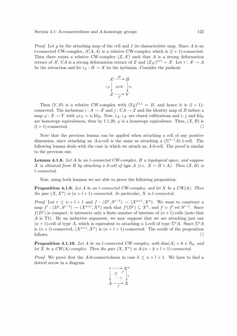
Section 4.1: A-connectedness and A-homotopy groups 122
Proof. Let g be the attaching map of the cell and f its characteristic map. Since A is anl-connected CW-complex, (CA,A) is a relative CW-complex which is (l + 1)-connected.Then there exists a relative CW-complex (Z,A′) such that A is a strong deformationretract of A′, CA is a strong deformation retract of Z and (ZA′)l+1 = A′. Let r : A′ → Abe the retraction and let iX : B → X be the inclusion. Consider the pushout
A′gr //
iA′push
B
iY
Zf ′// Y
Then (Y,B) is a relative CW-complex with (YB)l+1 = B, and hence it is (l + 1)-connected. The inclusions i : A→ A′ and j : CA→ Z and the identity map of B induce amap ϕ : X → Y with ϕiX = iY IdB. Now, iA, iA′ are closed cofibrations and i, j and IdBare homotopy equivalences, then by 1.1.20, ϕ is a homotopy equivalence. Thus, (X,B) is(l + 1)-connected.
Note that the previous lemma can be applied when attaching a cell of any positivedimension, since attaching an A-n-cell is the same as attaching a (Σn−1A)-1-cell. Thefollowing lemma deals with the case in which we attach an A-0-cell. The proof is similarto the previous one.
Lemma 4.1.8. Let A be an l-connected CW-complex, B a topological space, and supposeX is obtained from B by attaching a 0-cell of type A (i.e. X = B ∨ A). Then (X,B) isl-connected.
Now, using both lemmas we are able to prove the following proposition.
Proposition 4.1.9. Let A be an l-connected CW-complex, and let X be a CW(A). Thenthe pair (X,Xn) is (n+ l + 1)-connected. In particular, X is l-connected.
Proof. Let r ≤ n + l + 1 and f : (Dr, Sr−1) → (Xn+1, Xn). We want to construct amap f ′ : (Dr, Sr−1) → (Xn+1, Xn) such that f ′(Dr) ⊆ Xn, and f ' f ′ rel Sr−1. Sincef(Dr) is compact, it intersects only a finite number of interiors of (n+ 1)-cells (note thatA is T1). By an inductive argument, we may suppose that we are attaching just one(n + 1)-cell of type A, which is equivalent to attaching a 1-cell of type ΣnA. Since ΣnAis (n + l)-connected, (Xn+1, Xn) is (n + l + 1)-connected. The result of the propositionfollows.
Proposition 4.1.10. Let A be an l-connected CW-complex, with dim(A) = k ∈ N0, andlet X be a CW(A)-complex. Then the pair (X,Xn) is A-(n− k + l + 1)-connected.
Proof. We prove first the A-0-connectedness in case k ≤ n + l + 1. We have to find adotted arrow in a diagram
∗ //
'|‖
Xn
i
Af//
==
X
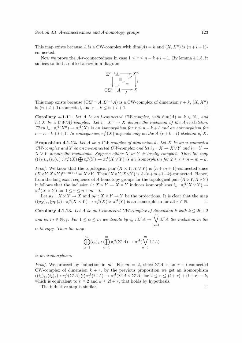
Section 4.1: A-connectedness and A-homotopy groups 123
This map exists because A is a CW-complex with dim(A) = k and (X,Xn) is (n+ l+ 1)-connected.
Now we prove the A-r-connectedness in case 1 ≤ r ≤ n− k+ l+ 1. By lemma 4.1.5, itsuffices to find a dotted arrow in a diagram
Σr−1A //
'|‖
Xn
i
CΣr−1A f
//
::
X
This map exists because (CΣr−1A,Σr−1A) is a CW-complex of dimension r + k, (X,Xn)is (n+ l + 1)-connected, and r + k ≤ n+ l + 1.
Corollary 4.1.11. Let A be an l-connected CW-complex, with dim(A) = k ∈ N0, andlet X be a CW(A)-complex. Let i : Xn → X denote the inclusion of the A-n-skeleton.Then i∗ : πAr (Xn) → πAr (X) is an isomorphism for r ≤ n− k + l and an epimorphism forr = n− k+ l+1. In consequence, πAr (X) depends only on the A-(r+ k− l)-skeleton of X.
Proposition 4.1.12. Let A be a CW-complex of dimension k. Let X be an n-connectedCW-complex and Y be an m-connected CW-complex and let iX : X → X∨Y and iY : Y →X ∨ Y denote the inclusions. Suppose either X or Y is locally compact. Then the map((iX)∗, (iY )∗) : πAr (X)
⊕πAr (Y ) → πAr (X ∨ Y ) is an isomorphism for 2 ≤ r ≤ n+m− k.
Proof. We know that the topological pair (X × Y,X ∨ Y ) is (n+m+ 1)-connected since(X×Y,X∨Y )(n+m+1) = X∨Y . Then (X×Y,X∨Y ) is A-(n+m+1−k)-connected. Hence,from the long exact sequence of A-homotopy groups for the topological pair (X×Y,X∨Y )it follows that the inclusion i : X ∨ Y → X × Y induces isomorphisms i∗ : πAr (X ∨ Y ) →πAr (X × Y ) for 1 ≤ r ≤ n+m− k.
Let pX : X × Y → X and pY : X × Y → Y be the projections. It is clear that the map((pX)∗, (pY )∗) : πAr (X × Y ) → πAr (X)× πAr (Y ) is an isomorphism for all r ∈ N.
Corollary 4.1.13. Let A be an l-connected CW-complex of dimension k with k ≤ 2l + 2
and let m ∈ N≥2. For 1 ≤ α ≤ m we denote by iα : ΣrA →m∨α=1
ΣrA the inclusion in the
α-th copy. Then the map
m⊕α=1
(iα)∗ :m⊕α=1
πAr (ΣrA) → πAr (m∨α=1
ΣrA)
is an isomorphism.
Proof. We proceed by induction in m. For m = 2, since ΣrA is an r + l-connectedCW-complex of dimension k + r, by the previous proposition we get an isomorphism((i1)∗, (i2)∗) : πAr (ΣrA)
⊕πAr (ΣrA) → πAr (ΣrA ∨ ΣrA) for 2 ≤ r ≤ (l + r) + (l + r) − k,
which is equivalent to r ≥ 2 and k ≤ 2l + r, that holds by hypothesis.The inductive step is similar.
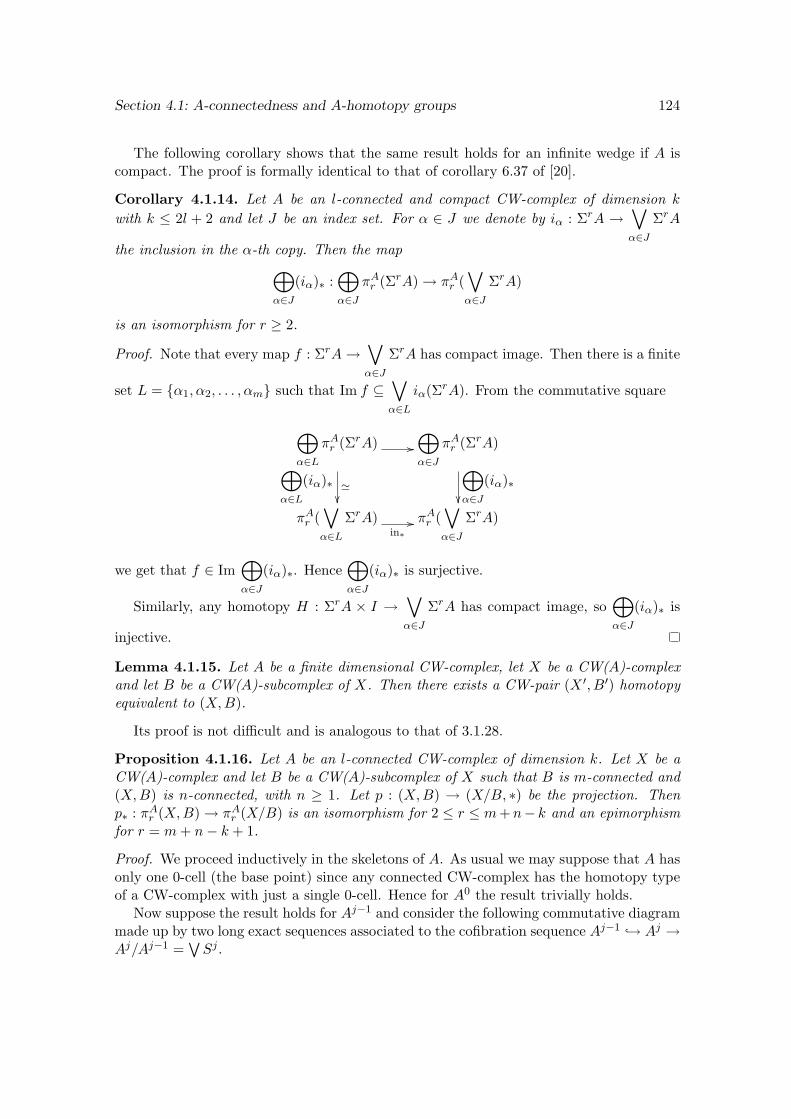
Section 4.1: A-connectedness and A-homotopy groups 124
The following corollary shows that the same result holds for an infinite wedge if A iscompact. The proof is formally identical to that of corollary 6.37 of [20].
Corollary 4.1.14. Let A be an l-connected and compact CW-complex of dimension k
with k ≤ 2l + 2 and let J be an index set. For α ∈ J we denote by iα : ΣrA →∨α∈J
ΣrA
the inclusion in the α-th copy. Then the map⊕α∈J
(iα)∗ :⊕α∈J
πAr (ΣrA) → πAr (∨α∈J
ΣrA)
is an isomorphism for r ≥ 2.
Proof. Note that every map f : ΣrA→∨α∈J
ΣrA has compact image. Then there is a finite
set L = α1, α2, . . . , αm such that Im f ⊆∨α∈L
iα(ΣrA). From the commutative square
⊕α∈L
πAr (ΣrA) //⊕α∈L
(iα)∗ '
⊕α∈J
πAr (ΣrA)⊕α∈J
(iα)∗
πAr (∨α∈L
ΣrA)in∗// πAr (∨α∈J
ΣrA)
we get that f ∈ Im⊕α∈J
(iα)∗. Hence⊕α∈J
(iα)∗ is surjective.
Similarly, any homotopy H : ΣrA × I →∨α∈J
ΣrA has compact image, so⊕α∈J
(iα)∗ is
injective.
Lemma 4.1.15. Let A be a finite dimensional CW-complex, let X be a CW(A)-complexand let B be a CW(A)-subcomplex of X. Then there exists a CW-pair (X ′, B′) homotopyequivalent to (X,B).
Its proof is not difficult and is analogous to that of 3.1.28.
Proposition 4.1.16. Let A be an l-connected CW-complex of dimension k. Let X be aCW(A)-complex and let B be a CW(A)-subcomplex of X such that B is m-connected and(X,B) is n-connected, with n ≥ 1. Let p : (X,B) → (X/B, ∗) be the projection. Thenp∗ : πAr (X,B) → πAr (X/B) is an isomorphism for 2 ≤ r ≤ m+n− k and an epimorphismfor r = m+ n− k + 1.
Proof. We proceed inductively in the skeletons of A. As usual we may suppose that A hasonly one 0-cell (the base point) since any connected CW-complex has the homotopy typeof a CW-complex with just a single 0-cell. Hence for A0 the result trivially holds.
Now suppose the result holds for Aj−1 and consider the following commutative diagrammade up by two long exact sequences associated to the cofibration sequence Aj−1 → Aj →Aj/Aj−1 =
∨Sj .
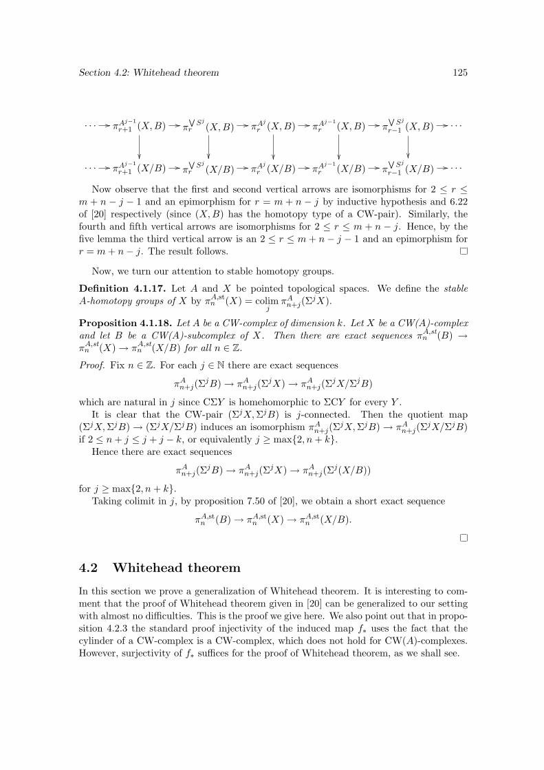
Section 4.2: Whitehead theorem 125
. . . // πAj−1
r+1 (X,B) //
πWSj
r (X,B) //
πAj
r (X,B) //
πAj−1
r (X,B) //
πWSj
r−1 (X,B) //
. . .
. . . // πAj−1
r+1 (X/B) // πWSj
r (X/B) // πAj
r (X/B) // πAj−1
r (X/B) // πWSj
r−1 (X/B) // . . .
Now observe that the first and second vertical arrows are isomorphisms for 2 ≤ r ≤m + n − j − 1 and an epimorphism for r = m + n − j by inductive hypothesis and 6.22of [20] respectively (since (X,B) has the homotopy type of a CW-pair). Similarly, thefourth and fifth vertical arrows are isomorphisms for 2 ≤ r ≤ m + n − j. Hence, by thefive lemma the third vertical arrow is an 2 ≤ r ≤ m+ n− j − 1 and an epimorphism forr = m+ n− j. The result follows.
Now, we turn our attention to stable homotopy groups.
Definition 4.1.17. Let A and X be pointed topological spaces. We define the stableA-homotopy groups of X by πA,stn (X) = colim
jπAn+j(Σ
jX).
Proposition 4.1.18. Let A be a CW-complex of dimension k. Let X be a CW(A)-complexand let B be a CW(A)-subcomplex of X. Then there are exact sequences πA,stn (B) →πA,stn (X) → πA,stn (X/B) for all n ∈ Z.
Proof. Fix n ∈ Z. For each j ∈ N there are exact sequences
πAn+j(ΣjB) → πAn+j(Σ
jX) → πAn+j(ΣjX/ΣjB)
which are natural in j since CΣY is homehomorphic to ΣCY for every Y .It is clear that the CW-pair (ΣjX,ΣjB) is j-connected. Then the quotient map
(ΣjX,ΣjB) → (ΣjX/ΣjB) induces an isomorphism πAn+j(ΣjX,ΣjB) → πAn+j(Σ
jX/ΣjB)if 2 ≤ n+ j ≤ j + j − k, or equivalently j ≥ max2, n+ k.
Hence there are exact sequences
πAn+j(ΣjB) → πAn+j(Σ
jX) → πAn+j(Σj(X/B))
for j ≥ max2, n+ k.Taking colimit in j, by proposition 7.50 of [20], we obtain a short exact sequence
πA,stn (B) → πA,stn (X) → πA,stn (X/B).
4.2 Whitehead theorem
In this section we prove a generalization of Whitehead theorem. It is interesting to com-ment that the proof of Whitehead theorem given in [20] can be generalized to our settingwith almost no difficulties. This is the proof we give here. We also point out that in propo-sition 4.2.3 the standard proof injectivity of the induced map f∗ uses the fact that thecylinder of a CW-complex is a CW-complex, which does not hold for CW(A)-complexes.However, surjectivity of f∗ suffices for the proof of Whitehead theorem, as we shall see.
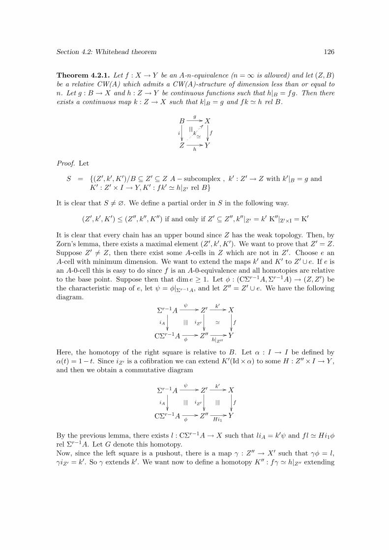
Section 4.2: Whitehead theorem 126
Theorem 4.2.1. Let f : X → Y be an A-n-equivalence (n = ∞ is allowed) and let (Z,B)be a relative CW(A) which admits a CW(A)-structure of dimension less than or equal ton. Let g : B → X and h : Z → Y be continuous functions such that h|B = fg. Then thereexists a continuous map k : Z → X such that k|B = g and fk ' h rel B.
Bg //
i '|‖
X
f
Zh//
k
>>
Y
Proof. Let
S = (Z ′, k′,K ′)/B ⊆ Z ′ ⊆ Z A− subcomplex , k′ : Z ′ → Z with k′|B = g andK ′ : Z ′ × I → Y,K ′ : fk′ ' h|Z′ rel B
It is clear that S 6= ∅. We define a partial order in S in the following way.
(Z ′, k′,K ′) ≤ (Z ′′, k′′,K ′′) if and only if Z ′ ⊆ Z ′′, k′′|Z′ = k′ K′′|Z′×I = K′
It is clear that every chain has an upper bound since Z has the weak topology. Then, byZorn’s lemma, there exists a maximal element (Z ′, k′,K ′). We want to prove that Z ′ = Z.Suppose Z ′ 6= Z, then there exist some A-cells in Z which are not in Z ′. Choose e anA-cell with minimum dimension. We want to extend the maps k′ and K ′ to Z ′ ∪ e. If e isan A-0-cell this is easy to do since f is an A-0-equivalence and all homotopies are relativeto the base point. Suppose then that dim e ≥ 1. Let φ : (CΣr−1A,Σr−1A) → (Z,Z ′) bethe characteristic map of e, let ψ = φ|Σr−1A, and let Z ′′ = Z ′ ∪ e. We have the followingdiagram.
Σr−1Aψ //
iA
Z ′k′ //
iZ′
X
f
CΣr−1A φ
//
|‖
Z ′′h|Z′′
//
'
Y
Here, the homotopy of the right square is relative to B. Let α : I → I be defined byα(t) = 1− t. Since iZ′ is a cofibration we can extend K ′(Id×α) to some H : Z ′′× I → Y ,and then we obtain a commutative diagram
Σr−1Aψ //
iA
Z ′k′ //
iZ′
X
f
CΣr−1A φ
//
|‖
Z ′′Hi1
//
|‖
Y
By the previous lemma, there exists l : CΣr−1A→ X such that liA = k′ψ and fl ' Hi1φrel Σr−1A. Let G denote this homotopy.Now, since the left square is a pushout, there is a map γ : Z ′′ → X ′ such that γφ = l,γiZ′ = k′. So γ extends k′. We want now to define a homotopy K ′′ : fγ ' h|Z′′ extending
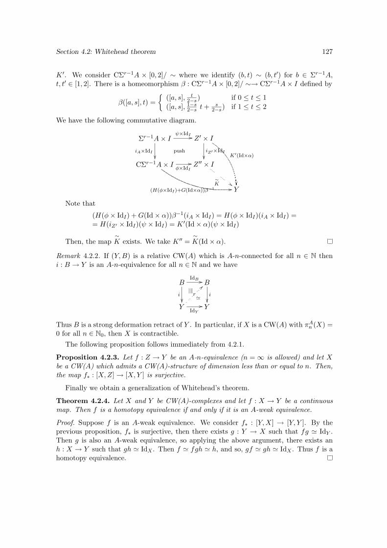
Section 4.2: Whitehead theorem 127
K ′. We consider CΣr−1A × [0, 2]/ ∼ where we identify (b, t) ∼ (b, t′) for b ∈ Σr−1A,t, t′ ∈ [1, 2]. There is a homeomorphism β : CΣr−1A× [0, 2]/ ∼→ CΣr−1A× I defined by
β([a, s], t) =
([a, s], t2−s) if 0 ≤ t ≤ 1
([a, s], 1−s2−s t+ s
2−s) if 1 ≤ t ≤ 2
We have the following commutative diagram.
Σr−1A× Iψ×IdI //
iA×IdI
Z ′ × I
iZ′×IdI
K′(Id×α)
CΣr−1A× Iφ×IdI
//
push
(H(φ×IdI)+G(Id×α))β−1 00
Z ′′ × I
∼K ##
Y
Note that
(H(φ× IdI) +G(Id× α))β−1(iA × IdI) = H(φ× IdI)(iA × IdI) == H(iZ′ × IdI)(ψ × IdI) = K ′(Id× α)(ψ × IdI)
Then, the map∼K exists. We take K ′′ =
∼K(Id× α).
Remark 4.2.2. If (Y,B) is a relative CW(A) which is A-n-connected for all n ∈ N theni : B → Y is an A-n-equivalence for all n ∈ N and we have
BIdB //
i '|‖
B
i
YIdY
//
r
>>
Y
Thus B is a strong deformation retract of Y . In particular, if X is a CW(A) with πAn (X) =0 for all n ∈ N0, then X is contractible.
The following proposition follows immediately from 4.2.1.
Proposition 4.2.3. Let f : Z → Y be an A-n-equivalence (n = ∞ is allowed) and let Xbe a CW(A) which admits a CW(A)-structure of dimension less than or equal to n. Then,the map f∗ : [X,Z] → [X,Y ] is surjective.
Finally we obtain a generalization of Whitehead’s theorem.
Theorem 4.2.4. Let X and Y be CW(A)-complexes and let f : X → Y be a continuousmap. Then f is a homotopy equivalence if and only if it is an A-weak equivalence.
Proof. Suppose f is an A-weak equivalence. We consider f∗ : [Y,X] → [Y, Y ]. By theprevious proposition, f∗ is surjective, then there exists g : Y → X such that fg ' IdY .Then g is also an A-weak equivalence, so applying the above argument, there exists anh : X → Y such that gh ' IdX . Then f ' fgh ' h, and so, gf ' gh ' IdX . Thus f is ahomotopy equivalence.
Chapter 5
Homology of CW(A)-complexes
In this chapter we start investigating the homology theory of CW(A)-complexes. Our maingoal is to develop tools and techniques which allow us to compute the singular homologyof these spaces out of the homology of the core A and the CW(A)-structure of the space.The tools we work with in this chapter are generalizations of classical cellular homology.
Note that the (reduced) homology of S0 (with coefficients in Z) has two significantproperties: it is concentrated in one degree (degree zero) and it is free (as an abeliangroup). Keeping this in mind, we study two cases: when the reduced homology of A isconcentrated in a certain degree and when the homology groups of A are free.
When the homology of the core A is neither concentrated nor free, the homology ofX is more difficult to compute. Example 5.2.8 of Section 3 shows that, in that case, thehomology of X cannot be computed from an A-cellular complex as in the other cases.However, in next chapter, we will study the general case by means of spectral sequences.
In the last section of this chapter we define and investigate the A-Euler characteristic χAof CW(A)-complexes, which is a homotopy invariant if A is a CW-complex with χ(A) 6= 0.We also define the multiplicative Euler characteristic when the core A has finite homology(see Theorem 5.3.8 below).
Throughout this chapter, homology will mean reduced homology with coefficients in Z.
5.1 Easy computations
As we claimed in the introduction, our aim is to compute the singular homology groupsof CW(A)-complexes out of the homology of A and the CW(A)-structure of the space.
Remark 5.1.1. Recall that if A and X are (pointed) CW-complexes and g : A → X is acontinuous (cellular) map there is a long exact sequence
. . . // Hn(A, ∗)g∗ // Hn(X, ∗)
i∗ // Hn(Cg, ∗)q∗ // Hn−1(A, ∗)
g∗ // . . .
which induces short exact sequences
0 // Coker g∗i∗ // Hn(Cg, ∗)
q∗ // Ker g∗ // 0
128
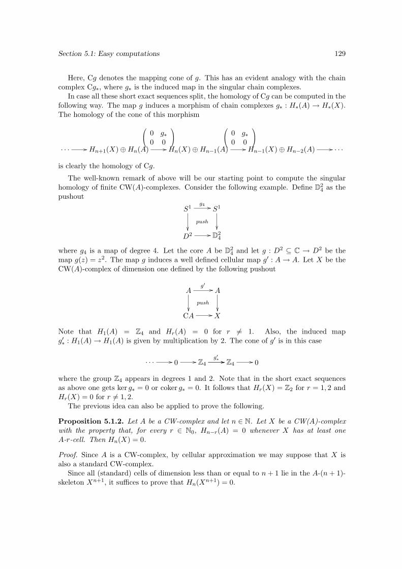
Section 5.1: Easy computations 129
Here, Cg denotes the mapping cone of g. This has an evident analogy with the chaincomplex Cg∗, where g∗ is the induced map in the singular chain complexes.
In case all these short exact sequences split, the homology of Cg can be computed in thefollowing way. The map g induces a morphism of chain complexes g∗ : H∗(A) → H∗(X).The homology of the cone of this morphism
. . . // Hn+1(X)⊕Hn(A)
0@ 0 g∗0 0
1A// Hn(X)⊕Hn−1(A)
0@ 0 g∗0 0
1A// Hn−1(X)⊕Hn−2(A) // . . .
is clearly the homology of Cg.
The well-known remark of above will be our starting point to compute the singularhomology of finite CW(A)-complexes. Consider the following example. Define D2
4 as thepushout
S1g4 //
push
S1
D2 // D24
where g4 is a map of degree 4. Let the core A be D24 and let g : D2 ⊆ C → D2 be the
map g(z) = z2. The map g induces a well defined cellular map g′ : A→ A. Let X be theCW(A)-complex of dimension one defined by the following pushout
Ag′ //
push
A
CA // X
Note that H1(A) = Z4 and Hr(A) = 0 for r 6= 1. Also, the induced mapg′∗ : H1(A) → H1(A) is given by multiplication by 2. The cone of g′ is in this case
. . . // 0 // Z4g′∗ //// Z4
// 0
where the group Z4 appears in degrees 1 and 2. Note that in the short exact sequencesas above one gets ker g∗ = 0 or coker g∗ = 0. It follows that Hr(X) = Z2 for r = 1, 2 andHr(X) = 0 for r 6= 1, 2.
The previous idea can also be applied to prove the following.
Proposition 5.1.2. Let A be a CW-complex and let n ∈ N. Let X be a CW(A)-complexwith the property that, for every r ∈ N0, Hn−r(A) = 0 whenever X has at least oneA-r-cell. Then Hn(X) = 0.
Proof. Since A is a CW-complex, by cellular approximation we may suppose that X isalso a standard CW-complex.
Since all (standard) cells of dimension less than or equal to n+ 1 lie in the A-(n+ 1)-skeleton Xn+1, it suffices to prove that Hn(Xn+1) = 0.
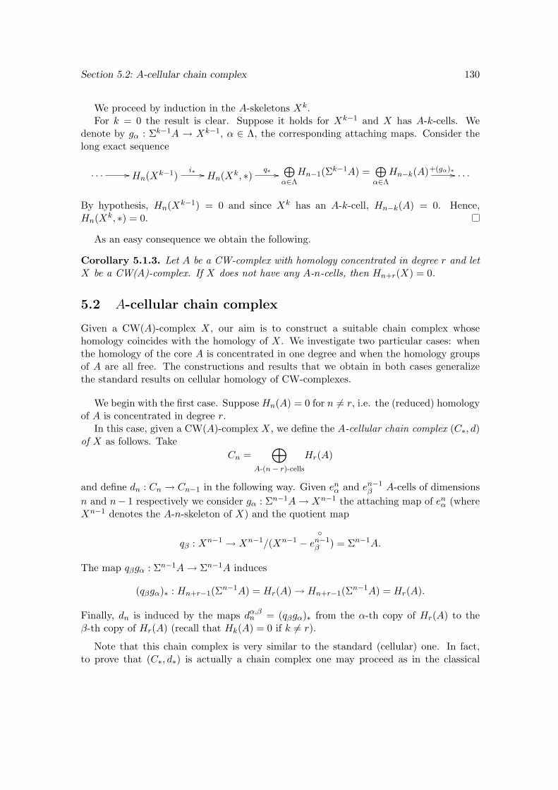
Section 5.2: A-cellular chain complex 130
We proceed by induction in the A-skeletons Xk.For k = 0 the result is clear. Suppose it holds for Xk−1 and X has A-k-cells. We
denote by gα : Σk−1A → Xk−1, α ∈ Λ, the corresponding attaching maps. Consider thelong exact sequence
. . . // Hn(Xk−1)i∗ // Hn(Xk, ∗)
q∗ //⊕α∈Λ
Hn−1(Σk−1A) =⊕α∈Λ
Hn−k(A)+(gα)∗ // . . .
By hypothesis, Hn(Xk−1) = 0 and since Xk has an A-k-cell, Hn−k(A) = 0. Hence,Hn(Xk, ∗) = 0.
As an easy consequence we obtain the following.
Corollary 5.1.3. Let A be a CW-complex with homology concentrated in degree r and letX be a CW(A)-complex. If X does not have any A-n-cells, then Hn+r(X) = 0.
5.2 A-cellular chain complex
Given a CW(A)-complex X, our aim is to construct a suitable chain complex whosehomology coincides with the homology of X. We investigate two particular cases: whenthe homology of the core A is concentrated in one degree and when the homology groupsof A are all free. The constructions and results that we obtain in both cases generalizethe standard results on cellular homology of CW-complexes.
We begin with the first case. Suppose Hn(A) = 0 for n 6= r, i.e. the (reduced) homologyof A is concentrated in degree r.
In this case, given a CW(A)-complex X, we define the A-cellular chain complex (C∗, d)of X as follows. Take
Cn =⊕
A-(n− r)-cells
Hr(A)
and define dn : Cn → Cn−1 in the following way. Given enα and en−1β A-cells of dimensions
n and n− 1 respectively we consider gα : Σn−1A→ Xn−1 the attaching map of enα (whereXn−1 denotes the A-n-skeleton of X) and the quotient map
qβ : Xn−1 → Xn−1/(Xn−1 −
en−1β ) = Σn−1A.
The map qβgα : Σn−1A→ Σn−1A induces
(qβgα)∗ : Hn+r−1(Σn−1A) = Hr(A) → Hn+r−1(Σn−1A) = Hr(A).
Finally, dn is induced by the maps dα,βn = (qβgα)∗ from the α-th copy of Hr(A) to theβ-th copy of Hr(A) (recall that Hk(A) = 0 if k 6= r).
Note that this chain complex is very similar to the standard (cellular) one. In fact,to prove that (C∗, d∗) is actually a chain complex one may proceed as in the classical
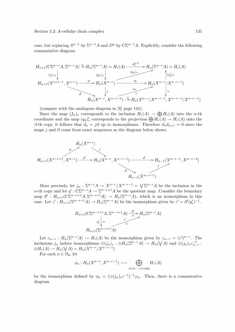
Section 5.2: A-cellular chain complex 131
case, but replacing Sn−1 by Σn−1A and Dn by CΣn−1A. Explicitly, consider the followingcommutative diagram
Hn+1(CΣn−rA,Σn−rA) ' //
(fα)∗
Hn(Σn−rA) = Hr(A)dα,β
n //
(gα)∗
Hn(Σn−rA) = Hr(A)
Hn+1(Xn+1−r, Xn−r) ∂ //
d′ ))TTTTTTTTTTTTTTTHn(Xn−r)
q∗ //
j
(qβ)∗33hhhhhhhhhhhhhhhhhhhh
Hn(Xn−r/Xn−r−1)
(q′β)∗
OO
'
Hn(Xn−r, Xn−r−1) ' //
ϕn
'
33hhhhhhhhhhhhhhhhhhhHn(Xn−r/Xn−r−1, Xn−r−1/Xn−r−1)
(compare with the analogous diagram in [8] page 141).Since the map (fα)∗ corresponds to the inclusion Hr(A) →
⊕Hr(A) into the α-th
coordinate and the map (qβ)′∗ corresponds to the projection⊕Hr(A) → Hr(A) onto the
β-th copy, it follows that dn = j∂ up to isomorphisms. Therefore dndn+1 = 0 since themaps j and ∂ come from exact sequences as the diagram below shows.
Hn(Xn−r)j
%%KKKKKKKKKK
Hn+1(Xn−r+1, Xn−r)
∂88rrrrrrrrrrd′ // Hn(Xn−r, Xn−r−1) d′ //
∂ &&NNNNNNNNNNNHn−1(Xn−r−1, Xn−r−2)
Hn−1(Xn−r−1)
j77nnnnnnnnnnnn
More precisely, let jα : Σn−rA → Xn−r/Xn−r−1 =∨
Σn−rA be the inclusion in theα-th copy and let q′ : CΣn−rA→ Σn−r+1A be the quotient map. Consider the boundarymap ∂′ : Hn+1(CΣn−r+1A,Σn−r+1A) → Hn(Σn−rA), which is an isomorphism in thiscase. Let ε′ : Hn+1(Σn−r+1A) → Hn(Σn−rA) be the isomorphism given by ε′ = ∂′(q′∗)
−1.
Hn+1(CΣn−r+1A,Σn−r+1A) ∂′
'//
q′∗ '
Hn(Σn−rA)
Hn+1(Σn−r+1A)
ε′
'
44jjjjjjjjjjjjjjjj
Let εn−r : Hn(Σn−rA) → Hr(A) be the isomorphism given by εn−r = (ε′)n−r. Theinclusions jα induce isomorphisms ⊕(jα)∗ : ⊕Hn(Σn−rA) → Hn(
∨A) and ⊕(jα)∗ε−1
n−r :⊕Hr(A) → Hn(
∨A) = Hn(Xn−r/Xn−r−1).
For each n ∈ N0, let
φn : Hn(Xn−r, Xn−r−1) −→⊕
A-(n− r)-cells
Hr(A)
be the isomorphism defined by φn = (⊕(jα)∗ε−1)−1ϕn. Then, there is a commutativediagram
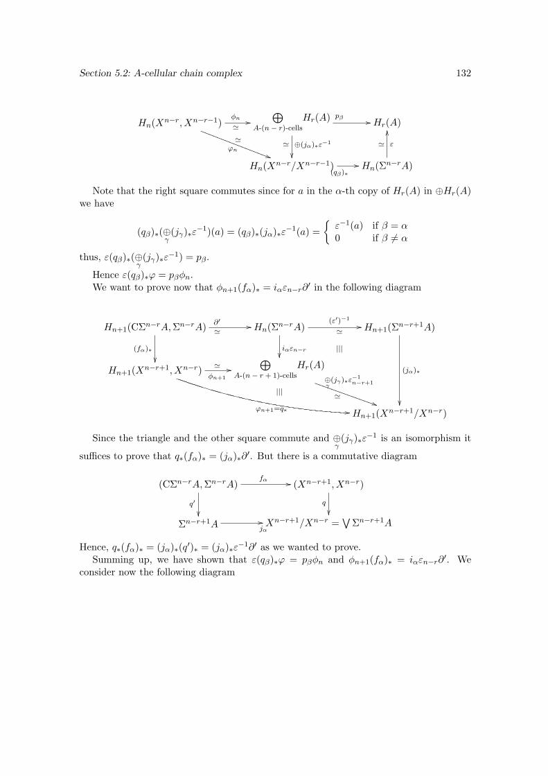
Section 5.2: A-cellular chain complex 132
Hn(Xn−r, Xn−r−1)φn
'//
'ϕn
))SSSSSSSSSSSSSSSSS
⊕A-(n− r)-cells
Hr(A) pβ //
' ⊕(jα)∗ε−1
Hr(A)
Hn(Xn−r/Xn−r−1)(qβ)∗
// Hn(Σn−rA)
ε'
OO
Note that the right square commutes since for a in the α-th copy of Hr(A) in ⊕Hr(A)we have
(qβ)∗(⊕γ(jγ)∗ε−1)(a) = (qβ)∗(jα)∗ε−1(a) =
ε−1(a) if β = α0 if β 6= α
thus, ε(qβ)∗(⊕γ(jγ)∗ε−1) = pβ.
Hence ε(qβ)∗ϕ = pβφn.We want to prove now that φn+1(fα)∗ = iαεn−r∂
′ in the following diagram
Hn+1(CΣn−rA,Σn−rA) ∂′
'//
(fα)∗
Hn(Σn−rA)
iαεn−r
(ε′)−1
'// Hn+1(Σn−r+1A)
(jα)∗
Hn+1(Xn−r+1, Xn−r)φn+1
' //
ϕn+1=q∗ ..
⊕A-(n− r + 1)-cells
Hr(A)⊕γ(jγ)∗ε
−1n−r+1
'))TTTTTTTTTTTTTTT
|||
|||
Hn+1(Xn−r+1/Xn−r)
Since the triangle and the other square commute and ⊕γ(jγ)∗ε−1 is an isomorphism it
suffices to prove that q∗(fα)∗ = (jα)∗∂′. But there is a commutative diagram
(CΣn−rA,Σn−rA)fα //
q′
(Xn−r+1, Xn−r)
q
Σn−r+1A jα
// Xn−r+1/Xn−r =∨
Σn−r+1A
Hence, q∗(fα)∗ = (jα)∗(q′)∗ = (jα)∗ε−1∂′ as we wanted to prove.Summing up, we have shown that ε(qβ)∗ϕ = pβφn and φn+1(fα)∗ = iαεn−r∂
′. Weconsider now the following diagram
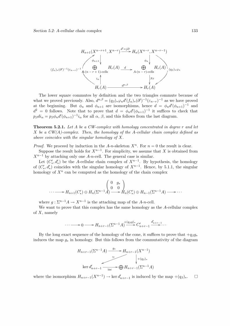
Section 5.2: A-cellular chain complex 133
Hn+1(Xn−r+1, Xn−r)d′=j∂ //
φn+1
Hn(Xn−r, Xn−r−1)
φn
(qβ)∗ϕn
yy
⊕A-(n− r + 1)-cells
Hr(A) d //⊕
A-(n− r)-cellsHr(A)
pβ
Hr(A) dα,β
//
(fα)∗(∂′)−1(εn−r)−1
99
iα
OO
Hr(A)
The lower square commutes by definition and the two triangles commute because ofwhat we proved previously. Also, dα,β = (qβ)∗ϕnd′(fα)∗(∂′)−1(εn−r)−1 as we have provedat the beginning. But φn and φn+1 are isomorphisms, hence d = φnd
′(φn+1)−1 andd2 = 0 follows. Note that to prove that d = φnd
′(φn+1)−1 it suffices to check thatpβdiα = pβφnd
′(φn+1)−1iα for all α, β, and this follows from the last diagram.
Theorem 5.2.1. Let A be a CW-complex with homology concentrated in degree r and letX be a CW(A)-complex. Then, the homology of the A-cellular chain complex defined asabove coincides with the singular homology of X.
Proof. We proceed by induction in the A-n-skeleton Xn. For n = 0 the result is clear.Suppose the result holds for Xn−1. For simplicity, we assume that X is obtained from
Xn−1 by attaching only one A-n-cell. The general case is similar.Let (C ′∗, d
′∗) be the A-cellular chain complex of Xn−1. By hypothesis, the homology
of (C ′∗, d′∗) coincides with the singular homology of Xn−1. Hence, by 5.1.1, the singular
homology of Xn can be computed as the homology of the chain complex
. . . // Hn+1(C ′∗)⊕Hn(Σn−1A)
0@ 0 g∗0 0
1A// Hn(C ′∗)⊕Hn−1(Σn−1A) // . . .
where g : Σn−1A→ Xn−1 is the attaching map of the A-n-cell.We want to prove that this complex has the same homology as the A-cellular complex
of X, namely
. . . // 0 // Hn+r−1(Σn−1A)+(qβg)∗// C ′n+r−1
d′n+r−1// . . .
By the long exact sequence of the homology of the cone, it suffices to prove that +qβg∗induces the map g∗ in homology. But this follows from the commutativity of the diagram
Hn+r−1(Σn−1A)g∗ // Hn+r−1(Xn−1)
+(qβ)∗
'
uukkkkkkkkkkkkkk
ker d′n+r−1 inc//⊕Hn+r−1(Σn−1A)
where the isomorphism Hn+r−1(Xn−1) → ker d′n+r−1 is induced by the map +(qβ)∗.
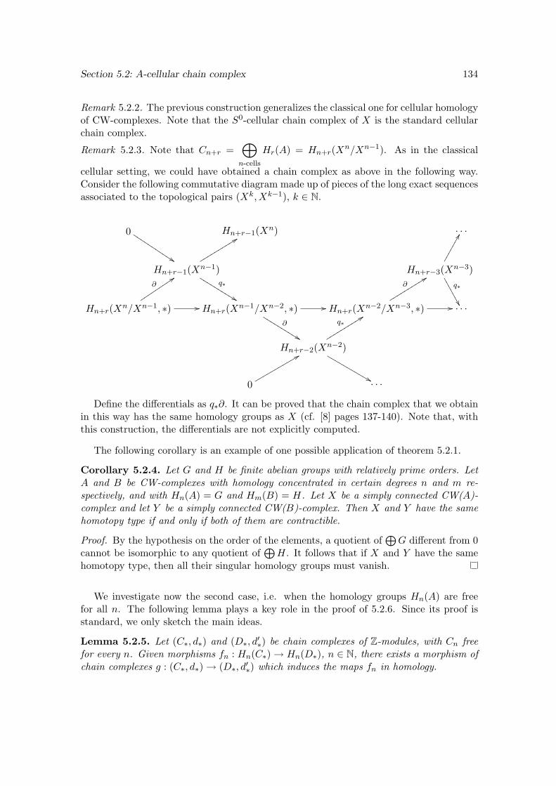
Section 5.2: A-cellular chain complex 134
Remark 5.2.2. The previous construction generalizes the classical one for cellular homologyof CW-complexes. Note that the S0-cellular chain complex of X is the standard cellularchain complex.
Remark 5.2.3. Note that Cn+r =⊕n-cells
Hr(A) = Hn+r(Xn/Xn−1). As in the classical
cellular setting, we could have obtained a chain complex as above in the following way.Consider the following commutative diagram made up of pieces of the long exact sequencesassociated to the topological pairs (Xk, Xk−1), k ∈ N.
0
$$JJJJJJJJJJJ Hn+r−1(Xn) . . .
Hn+r−1(Xn−1)q∗
%%KKKKKKKKKK
99ssssssssssHn+r−3(Xn−3)
q∗
111
1111
FF
Hn+r(Xn/Xn−1, ∗) //
∂::ttttttttt
Hn+r(Xn−1/Xn−2, ∗) //
∂
%%KKKKKKKKKKHn+r(Xn−2/Xn−3, ∗) //
∂99ssssssssss
. . .
Hn+r−2(Xn−2)
q∗99ssssssssss
&&LLLLLLLLLLL
0
88rrrrrrrrrrr . . .
Define the differentials as q∗∂. It can be proved that the chain complex that we obtainin this way has the same homology groups as X (cf. [8] pages 137-140). Note that, withthis construction, the differentials are not explicitly computed.
The following corollary is an example of one possible application of theorem 5.2.1.
Corollary 5.2.4. Let G and H be finite abelian groups with relatively prime orders. LetA and B be CW-complexes with homology concentrated in certain degrees n and m re-spectively, and with Hn(A) = G and Hm(B) = H. Let X be a simply connected CW(A)-complex and let Y be a simply connected CW(B)-complex. Then X and Y have the samehomotopy type if and only if both of them are contractible.
Proof. By the hypothesis on the order of the elements, a quotient of⊕G different from 0
cannot be isomorphic to any quotient of⊕H. It follows that if X and Y have the same
homotopy type, then all their singular homology groups must vanish.
We investigate now the second case, i.e. when the homology groups Hn(A) are freefor all n. The following lemma plays a key role in the proof of 5.2.6. Since its proof isstandard, we only sketch the main ideas.
Lemma 5.2.5. Let (C∗, d∗) and (D∗, d′∗) be chain complexes of Z-modules, with Cn freefor every n. Given morphisms fn : Hn(C∗) → Hn(D∗), n ∈ N, there exists a morphism ofchain complexes g : (C∗, d∗) → (D∗, d′∗) which induces the maps fn in homology.
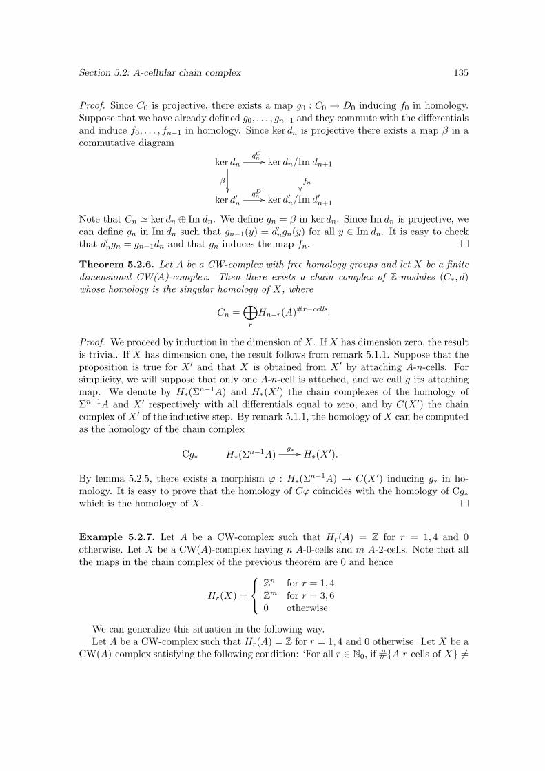
Section 5.2: A-cellular chain complex 135
Proof. Since C0 is projective, there exists a map g0 : C0 → D0 inducing f0 in homology.Suppose that we have already defined g0, . . . , gn−1 and they commute with the differentialsand induce f0, . . . , fn−1 in homology. Since ker dn is projective there exists a map β in acommutative diagram
ker dnqCn //
β
ker dn/Im dn+1
fn
ker d′n
qDn // ker d′n/Im d′n+1
Note that Cn ' ker dn ⊕ Im dn. We define gn = β in ker dn. Since Im dn is projective, wecan define gn in Im dn such that gn−1(y) = d′ngn(y) for all y ∈ Im dn. It is easy to checkthat d′ngn = gn−1dn and that gn induces the map fn.
Theorem 5.2.6. Let A be a CW-complex with free homology groups and let X be a finitedimensional CW(A)-complex. Then there exists a chain complex of Z-modules (C∗, d)whose homology is the singular homology of X, where
Cn =⊕r
Hn−r(A)#r−cells.
Proof. We proceed by induction in the dimension of X. If X has dimension zero, the resultis trivial. If X has dimension one, the result follows from remark 5.1.1. Suppose that theproposition is true for X ′ and that X is obtained from X ′ by attaching A-n-cells. Forsimplicity, we will suppose that only one A-n-cell is attached, and we call g its attachingmap. We denote by H∗(Σn−1A) and H∗(X ′) the chain complexes of the homology ofΣn−1A and X ′ respectively with all differentials equal to zero, and by C(X ′) the chaincomplex of X ′ of the inductive step. By remark 5.1.1, the homology of X can be computedas the homology of the chain complex
Cg∗ H∗(Σn−1A)g∗ // H∗(X ′).
By lemma 5.2.5, there exists a morphism ϕ : H∗(Σn−1A) → C(X ′) inducing g∗ in ho-mology. It is easy to prove that the homology of Cϕ coincides with the homology of Cg∗which is the homology of X.
Example 5.2.7. Let A be a CW-complex such that Hr(A) = Z for r = 1, 4 and 0otherwise. Let X be a CW(A)-complex having n A-0-cells and m A-2-cells. Note that allthe maps in the chain complex of the previous theorem are 0 and hence
Hr(X) =
Zn for r = 1, 4Zm for r = 3, 60 otherwise
We can generalize this situation in the following way.Let A be a CW-complex such that Hr(A) = Z for r = 1, 4 and 0 otherwise. Let X be a
CW(A)-complex satisfying the following condition: ‘For all r ∈ N0, if #A-r-cells of X 6=
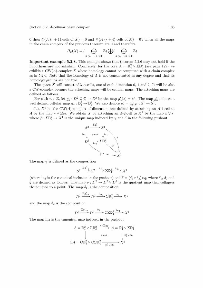
Section 5.2: A-cellular chain complex 136
0 then #A-(r + 1)-cells of X = 0 and #A-(r + 4)-cells of X = 0’. Then all the mapsin the chain complex of the previous theorem are 0 and therefore
Hn(X) = (⊕
A-(n− 1)-cells
Z)⊕
(⊕
A-(n− 4)-cells
Z)
Important example 5.2.8. This example shows that theorem 5.2.6 may not hold if thehypothesis are not satisfied. Concretely, for the core A = D2
4 ∨ ΣD24 (see page 129) we
exhibit a CW(A)-complex X whose homology cannot be computed with a chain complexas in 5.2.6. Note that the homology of A is not concentrated in any degree and that itshomology groups are not free.
The space X will consist of 3 A-cells, one of each dimension 0, 1 and 2. It will be alsoa CW-complex because the attaching maps will be cellular maps. The attaching maps aredefined as follows.
For each n ∈ Z, let g′n : D2 ⊆ C → D2 be the map g′n(z) = zn. The map g′n induces awell defined cellular map gn : D2
4 → D24. We also denote g′n = g′n|S1 : S1 → S1.
Let X1 be the CW(A)-complex of dimension one defined by attaching an A-1-cell toA by the map ∗ ∨ Σg2. We obtain X by attaching an A-2-cell to X1 by the map β ∨ ∗,where β : ΣD2
4 → X1 is the unique map induced by γ and δ in the following pushout
S2Σg′4 //
inc
push
S2
in1
γ
D3in2
//
δ //
ΣD24
β
!!DDD
DDDD
D
X1
The map γ is defined as the composition
S2Σg′−2 // S2
in1 // ΣD24
in3 // X1
(where in3 is the canonical inclusion in the pushout) and δ = (δ1∨ δ2)q, where δ1, δ2 andq are defined as follows. The map q : D2 → D2 ∨D2 is the quotient map that collapsesthe equator to a point. The map δ1 is the composition
D3Σg′−1 // D3
in2 // ΣD24
in3 // X1
and the map δ2 is the composition
D3Σg′−2 // D3
Cin1 // CΣD24
in4 // X1
The map in4 is the canonical map induced in the pushout
A = D24 ∨ ΣD2
4
∗∨Σg2 //
push
A = D24 ∨ ΣD2
4
in′3∨in3
CA = CD2
4 ∨ CΣD24 in′4∨in4
// X1
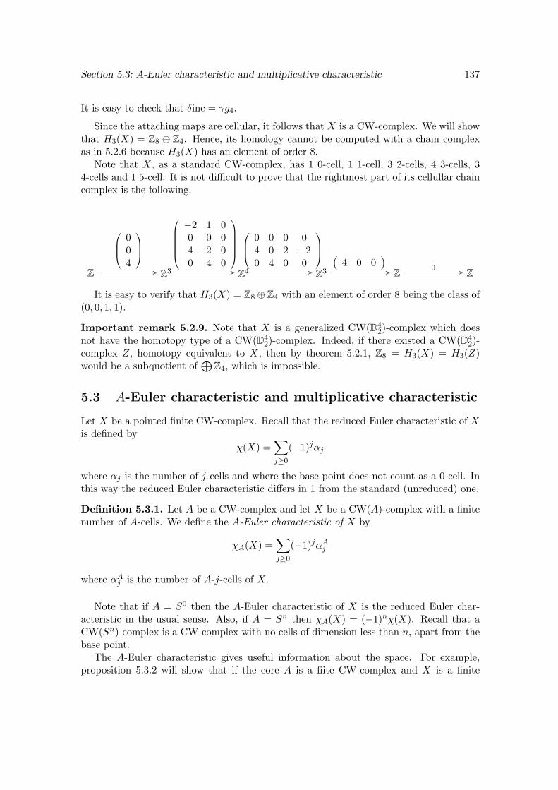
Section 5.3: A-Euler characteristic and multiplicative characteristic 137
It is easy to check that δinc = γg4.
Since the attaching maps are cellular, it follows that X is a CW-complex. We will showthat H3(X) = Z8 ⊕ Z4. Hence, its homology cannot be computed with a chain complexas in 5.2.6 because H3(X) has an element of order 8.
Note that X, as a standard CW-complex, has 1 0-cell, 1 1-cell, 3 2-cells, 4 3-cells, 34-cells and 1 5-cell. It is not difficult to prove that the rightmost part of its cellullar chaincomplex is the following.
Z
0BB@004
1CCA// Z3
0BBBBB@−2 1 00 0 04 2 00 4 0
1CCCCCA// Z4
0BB@0 0 0 04 0 2 −20 4 0 0
1CCA// Z3
“4 0 0
”// Z 0 // Z
It is easy to verify that H3(X) = Z8 ⊕Z4 with an element of order 8 being the class of(0, 0, 1, 1).
Important remark 5.2.9. Note that X is a generalized CW(D42)-complex which does
not have the homotopy type of a CW(D42)-complex. Indeed, if there existed a CW(D4
2)-complex Z, homotopy equivalent to X, then by theorem 5.2.1, Z8 = H3(X) = H3(Z)would be a subquotient of
⊕Z4, which is impossible.
5.3 A-Euler characteristic and multiplicative characteristic
Let X be a pointed finite CW-complex. Recall that the reduced Euler characteristic of Xis defined by
χ(X) =∑j≥0
(−1)jαj
where αj is the number of j-cells and where the base point does not count as a 0-cell. Inthis way the reduced Euler characteristic differs in 1 from the standard (unreduced) one.
Definition 5.3.1. Let A be a CW-complex and let X be a CW(A)-complex with a finitenumber of A-cells. We define the A-Euler characteristic of X by
χA(X) =∑j≥0
(−1)jαAj
where αAj is the number of A-j-cells of X.
Note that if A = S0 then the A-Euler characteristic of X is the reduced Euler char-acteristic in the usual sense. Also, if A = Sn then χA(X) = (−1)nχ(X). Recall that aCW(Sn)-complex is a CW-complex with no cells of dimension less than n, apart from thebase point.
The A-Euler characteristic gives useful information about the space. For example,proposition 5.3.2 will show that if the core A is a fiite CW-complex and X is a finite
Section 5.3: A-Euler characteristic and multiplicative characteristic 138
CW(A)-complex then χ(X) can be computed from χ(A) and χA(X). Note that χ(X) iswell defined since X has the homotopy type of a finite CW-complex. When χ(A) 6= 0,the A-Euler characteristic is a homotopical invariant. In case χ(A) = 0, it might not beinvariant by homotopy equivalences or even homeomorphisms, as the following exampleshows.
Take the core A as D1 (with 1 as base point). The disk D2 is homeomorphic to CA andΣA. We know that CA is obtained from A by attaching an A-1-cell, hence χA(CA) = 0.On the other hand, ΣA is obtained from ∗ by attaching a A-1-cell, so χA(ΣA) = −1.Note that there are A-cellular approximations to the identity map of D2 between thesetwo different A-cellular structures, and that the homology of D2 can be computed fromthe A-cellular complex by 5.2.1. But in this case the A-Euler characteristic cannot becomputed from the A-cellular complex since, in contrast to the classical situation wherethe cellular complex has a copy of Z for each cell, the A-cellular complex has a trivialgroup for each A-cell of D2.
Nevertheless the A-Euler characteristic gives us very useful information about the space.The following proposition shows that if the core A is a finite CW-complex and X is a finiteCW(A)-complex then χ(X) can be computed from χ(A) and χA(X). Note that χ(X) iswell defined since X has the homotopy type of a finite CW-complex.
Proposition 5.3.2. Let A be a finite CW-complex and let X be a finite CW(A)-complex.Then χ(X) = χA(X)χ(A).
Proof. The proposition follows from the fact that, for all n ∈ N0 the relative CW-complexes(CΣnA,ΣnA) have exactly the same cells as A but shifted in dimension. Note also thatX has the homotopy type of a CW-complex X ′ which is obtained by approximating theattaching maps of X by cellular maps.
Corollary 5.3.3. If χ(A) 6= 0 and χA(X) 6= 0 then X is not contractible.
Note that in case A = Sn the corollary does not say anything new. But, for example,if A is a torus (χ(A) = −1) and X is a CW(A)-complex with an odd number of cells, thenX is not contractible. Also, in this case, if X has any number of cells but only in evendimensions, it cannot be contractible.
We study now another interesting case: when the homology of A is a finite gradedgroup.
We say that graded group (Gn)n∈N0 is finite if only a finite number of groups are nontrivial and all of them are finite. In a similar way we say that a chain complex of abeliangroups is finite if the underlying graded group is finite.
Definition 5.3.4. Let G = (Gn)n∈N0 be a finite graded group. We define the multiplicativeEuler characteristic of G as
χm(G) =∏n≥0
#(Gn)(−1)n
Section 5.3: A-Euler characteristic and multiplicative characteristic 139
Let C = (C∗, d∗) be a chain complex of abelian groups whose underlying graded groupis finite. Since Hn(C) = ker dn/Im dn+1 and Cn/ ker dn = Im dn, then
#Hn(C) = # ker dn/#Im dn+1 and #Cn = # ker dn.#Im dn.
It follows that∏n≥0
#(Hn(C))(−1)n=∏n even
# ker dn.#Im dn/∏n odd
# ker dn.#Im dn =∏n≥0
#(Cn)(−1)n
Therefore, the multiplicative Euler characteristic of C coincides with the multiplicativeEuler characteristic of the graded group H∗(C). In particular, the multiplicative Eulercharacteristic is invariant by quasi isomorphisms.
Example 5.3.5. Let (C∗, d∗) be a chain complex with Cn =⊕i∈In
Z4 for all n (where In
is any index set). Let (D∗, d′∗) be a chain complex with Hk(D) = Z2 for some k andHr(D) = 0 for r 6= k. Then C and D are not quasi isomorphic, because χm(C) = 4m forsome m ∈ Z, while χm(D) = 2 or χm(D) = 1
2 .
We may also ask whether the converse is true. Namely, given finite abelian groupsG1, . . . , Gk with
∏n≥0 #(Gn)(−1)n
= 4m for some m, can we find a chain complex ofabelian groups (C∗, d∗) with Cn =
⊕i∈In
Z4 for all n such that Hn(C) = Gn for n = 1, . . . , k
and Hn(C) = 0 in other case? For example, given m ∈ N, can we construct a chaincomplex (C∗, d∗) with Cn =
⊕j∈Jn
Z4 for all n such that Hk(C) = Z4m for some k and
Hr(C) = 0 for r 6= k?
The answer to this question is negative. For instance, if Hk(C) = Z16, then it containsan element of order 16 which cannot be obtained by taking a quotient of a subspace of⊕j∈Jn
Z4.
Remark 5.3.6. Let C = (Cn)n∈N0 , D = (Dn)n∈N0 and E = (En)n∈N0 be finite gradedgroups. It is easy to prove that if for each n there exists a short exact sequence
0 → Cn → Dn → En → 0
then χm(D) = χm(C)χm(E).The same holds in case there is an exact sequence
. . .→ En+1 → Cn → Dn → En → Cn−1 → . . .
for if we call this complex B, we have χm(B) = χm(H∗(B)) = 1 and clearly χm(B) =χm(C)χm(E)/χm(D).
Definition 5.3.7. Let X be a topological space with finite homology. We define themultiplicative Euler characteristic of X as the multiplicative Euler characteristic ofH∗(X).
Section 5.3: A-Euler characteristic and multiplicative characteristic 140
Theorem 5.3.8. Let A be a CW-complex with finite homology and let X be a finiteCW(A)-complex. Then
χm(X) =∏n≥0
χm(A)(−1)n#A-n-cells = χm(A)χA(X)
Proof. We proceed by induction in the number of cells of X. If X has only one cell thetheorem trivially holds. Suppose the result is true for X ′ and suppose X is obtained fromX ′ by attaching an A-r-cell. There exists a long exact sequence
. . . // Hn(Σr−1A, ∗) // Hn(X ′, ∗) // Hn(X, ∗) // Hn−1(Σr−1A, ∗) // . . .
Then, by 5.3.6,
χm(X ′) = χm(H∗(X ′)) = χm(H∗(Σr−1A))χm(H∗(X)) == χm(H∗(A))(−1)r−1
χm(H∗(X)) = χm(A)(−1)r−1χm(X)
So, χm(X) = χm(X ′)χm(A)(−1)r.
Example 5.3.9. Let A be a CW-complex with H1(A) = Z4 and Hr(A) = 0 for r 6= 1.Let X be a topological space with Hk(A) = Z2 for some k and Hr(A) = 0 for r 6= k. ThenX does not have the homotopy type of a CW(A)-complex.
The next result follows immediately from 5.3.8.
Proposition 5.3.10. Let A and B be CW-complexes with finite homology. Let X be atopological space with finite homology such that χm(X) 6= 1. Suppose, in addition, that Xcan be given both CW(A) and CW(B) structures. Then there exist k, l ∈ Z − 0 suchthat χm(A)k = χm(B)l.
Example 5.3.11 (Moore spaces). Fix a core A. Some questions that arise naturally arethe following. For which abelian groups G and n ∈ N does there exist a CW(A)-complexX such that Hn(X) = G and Hr(X) = 0 if r 6= n? Or more generally, for which sequencesof abelian groups (Gn)n∈N0 does there exist a CW(A)-complex X such that Hn(X) = Gnfor all n?
For example, if the core A is a simply-connected CW-complex with Hr(A) = Z forr = n and Hr(A) = 0 in other case, then A is homotopy equivalent to Sn. We knowthat for any abelian group G and for any k ≥ n there exists a CW-complex Z such thatHk(Z) = G and Hr(Z) = 0 if r 6= k. Hence, by 3.3.1, there exists a CW(A)-complex Xsuch that X has the same homology groups as Z.
Therefore, in this particular case, for any sequence of abelian groups (Gj)j≥n thereexists a CW(A)-complex X such that Hj(X) = Gj for all j ≥ n.
If A is a CW-complex with finite homology, the results of above provide necessaryconditions for the required CW(A)-complex X to exist. For instance, 5.3.8 settles aneasy-to-check necessary condition, as example 5.3.9 shows. In the case A = D2
4 (see page129), we cannot construct a CW(A)-complex X such that Hn(X) = Z5 for some n ∈ Nsince, by 5.2.1, Hn(X) must be a quotient of a subgroup of
⊕Z4.
We will continue studying these questions in chapter 7, where we will give some veryinteresting partial anwers to them.
Chapter 6
Applications of spectral sequencesto CW(A)-complexes
One basic and fundamental idea in topology is to study homotopical and homologicalproperties of a topological space by decomposing it into smaller parts. Since a CW(A)-complex is built up out of A-cells, one expects that its homotopical properties will dependheavily on the homotopy type of A. Our aim in this chapter is to develop methods tocompute homotopy and homology groups of a CW(A)-complex X from those of A andthe CW(A)-structure of X generalizing those in the previous chapter. It is evident thatthe skeletal filtration plays an important role and it seems quite natural that spectralsequences are the right tool to work with. For example, from the skeletal filtration of aCW(A)-complex X we will construct a spectral sequence which converges to the singularhomology groups of X.
Moreover, as one might expect, the homotopy groups of a CW(A)-complex X arestrongly related to those of A, although in general explicit computation seems to be hardwork. However, we obtain results which show how the homotopy groups of X depend onthose of A.
In the first section, given a CW-complex A we define a reduced homology theory onthe category of CW-complexes, called A-homology, which coincides with classical singularhomology in case A = S0. One of the most interesting results is a generalization ofHurewicz theorem (6.1.5), which gives a relationship between A-homology groups andA-homotopy groups.
In section 2 we study homotopy and homology of CW-complexes by means of spectralsequences and Serre classes obtaining many interesting results. Moreover, we introduce ageneralization of Serre classes which is suitable for working with CW(A)-complexes.
Finally, in the last section we derive some applications to real projective spaces
6.1 A-homology and A-homotopy
In this section we will define anA-shaped homology theory, which we callA-homology. Thisis a reduced homology theory which not only generalizes the classical singular homologytheory, but also satisfies nice properties such as a Hurewicz-type theorem (6.1.5).
141
Section 6.1: A-homology and A-homotopy 142
Definition 6.1.1. Let p : (E, e0) → (B, b0) be a continuous map and let F = p−1(b0). Wesay that p is an A-quasi-fibration if it induces isomorphisms p∗ : πAi (E,F, e0) → πAi (B, b0)for all i ∈ N, where πAi (E,F, e0) = [(CΣi−1A,Σi−1A, a0), (E,F, e0)].
Let ce0 and cb0 denote the constant loops at e0 and b0 respectively. Recall that, forany space A, πAi (B, b0) = πAi−1(ΩB, cb0) and πAi (E,F, e0) = πAi−1(P (E, e0, F ), ce0). Sincea weak equivalence is also an A-weak equivalence if A is a CW-complex, we deduce thefollowing.
Lemma 6.1.2. If p is a quasifibration and A is a CW-complex, then p is an A-quasi-fibration.
We define the A-homology groups inspired by the Dold-Thom theorem.
Definition 6.1.3. Let A be a CW-complex and let X be a topological space. For n ∈ N0
we define the n-th A-homology group of X as
HAn (X) = πAn (SP (X))
where SP (X) denotes the infinite symmetric product of X.
Theorem 6.1.4. The functor HA∗ (–) defines a reduced homology theory on the category
of (path-connected) CW-complexes.
Proof. It is clear that HA∗ (–) is a homotopy functor. If (X,B, x0) is a pointed CW-pair,
then by the Dold-Thom theorem, the quotient map q : X → X/B induces a quasifibrationq : SP (X) → SP (X/B) whose fiber is homotopy equivalent to SP (B). Then there is along exact sequence
. . . // πAn (SP (B)) // πAn (SP (X)) // πAn (SP (X/B)) // πAn−1(SP (B)) // . . .
It remains to show that there is a natural isomorphism HAn (X) ' HA
n+1(ΣX) and thatHAn (X) are abelian groups for n = 0, 1. The natural isomorphism follows from the long
exact sequence of above applied to the CW-pair (CX,X). Note that HAn (CX) = 0 since
CX is contractible and HAn is a homotopy functor. The second part follows immediately,
since HA0 (X) ' HA
1 (ΣX) ' HA2 (Σ2X). The group structure on HA
0 (X) is induced fromthe one on HA
1 (X) by the corresponding natural isomorphism.
Theorem 6.1.5. Let A be a path-connected CW-complex of dimension k ≥ 1 and let Xbe an n-connected topological space (with n ≥ k). Then HA
r (X) = 0 for r ≤ n − k andπAn−k+1(X) ' HA
n−k+1(X).
Proof. By Hurewicz, Hr(X) = 0 for r ≤ n and Hn+1(X) ' πn+1(X). Hence SP (X)is n-connected. Since dimA = k, it follows that SP (X) is A-(n − k)-connected. Thus,HAr (X) = 0 for r ≤ n− k. Also,
πAn−k+1(X) = [Σn−k+1A,X] ' Hn+1(Σn−k+1A, πn+1(X)) '' Hn+1(Σn−k+1A,Hn+1(X)) ' Hn+1(Σn−k+1A, πn+1(SP (X))) '' [Σn−k+1A,SP (X)] = πAn−k+1(SP (X)) = HA
n−k+1(X)
where the first and fourth isomorphisms hold by 2.5.6.
Section 6.1: A-homology and A-homotopy 143
Federer’s spectral sequence provides a first method of computation of A-homologygroups. Given CW-complexes A and X with A finite and H1(X) = 0, the associatedFederer spectral sequence Eap,q converges to the A-homotopy groups of SP (X) (notethat SP (X) is simply-connected). In this case we have E2
p,q = H−p(A, πq(SP (X))) =H−p(A,Hq(X)) if p+ q ≥ 1 and p ≤ −1 .
We exhibit now some examples.
Example 6.1.6. If A is a finite CW-complex and X is a Moore space of type (G,n) thenSP (X) is an Eilenberg-MacLane space of the same type. Note that SP (X) is abelian.Hence, by the Federer spectral sequence
HAr (X) = πAr (SP (X)) = Hn−r(A, πn(SP (X))) = Hn−r(A,G) for r ≥ 1.
In particular, HAr (Sn) = Hn−r(A,Z).
We also deduce that if X is a Moore space of type (G,n) and A is (n− 1)-connected,then HA
r (X) = 0 for all r ≥ 1.
Example 6.1.7. Let A be a Moore space of type (G,m) (with G finitely generated) andlet X be a path-connected abelian topological space. As in example 2.5.5, for n ≥ 1, thereare short exact sequences of abelian groups
0 // Ext(G,Hn+m+1(X)) // HAn (X) // Hom(G,Hn+m(X)) // 0
As a consequence, if G is a finite group of exponent r, α2r = 0 for every α ∈ HAn (X).
Using 6.1.6 we will show now a explicit formula to compute A-homology groups.
Proposition 6.1.8. Let A be a finite CW-complex and let X be a connected CW-complex.Then for every n ∈ N0, HA
n (X) =⊕j∈N
Hj−n(A,Hj(X)).
Proof. By corollary 4K.7 of [8], SP (X) has the weak homotopy type of∏n∈N
K(Hn(X), n).
Also, since A is a CW-complex, a weak equivalence is also an A-weak equivalence. Hence,
HAn (X) = πAn (SP (X)) = πAn (
∏j∈N
K(Hj(X), j)) =∏j∈N
πAn (K(Hj(X), j)) =
=∏j∈N
Hj−n(A,Hj(X)) =⊕j∈N
Hj−n(A,Hj(X))
where the first equality of the second line follows from 6.1.6 since for every group G andm ∈ N, SP (M(G,m)) is a K(G,m).
Now we show that, in case A is compact, HA∗ satisfies the wedge axiom. This can
be proved in two different ways: using the definition of A-homotopy groups or using theabove formula. We choose the first one.
Section 6.2: Homology and homotopy of CW(A)-complexes 144
Proposition 6.1.9. Let A be a finite CW-complex, and let Xii∈I be a collection ofCW-complexes. Then
HAn
(∨i∈I
Xi
)=⊕i∈I
HAn (Xi).
Proof. It is known that SP (∨i∈IXi) =
∏i∈I
wSP (Xi) with the weak product topology, i.e. the
colimit of the products of finitely many factors. Since A is compact, πAn (∏i∈I
wSP (Xi)) =⊕i∈IπAn (SP (Xi)) and the result follows.
Recall that a nonempty class of abelian groups C is called a Serre class if for any threeterm exact sequence A → B → C, if A,C ∈ C then B ∈ C . A Serre class C is called anacyclic ring of abelian groups if A ⊗ B and Tor(A,B) belong to C whenever A,B ∈ C .A morphism ϕ : G → H between abelian groups is called a C -isomorphism if both kerϕand cokerϕ belong to C . A topological space X is called C -acyclic if Hn(X) ∈ C for alln ≥ 1. We will introduce below the notion of special Serre class (6.2.5) which is a morerestrictive concept that we will need to deal with non-finite CW(A)-complexes.
Henceforward, C will denote a Serre class of abelian groups unless specified otherwise.
Proposition 6.1.10. Let A be a finite CW-complex and let k ∈ N. Let X be a topologicalspace such that πn(X) ∈ C for all n ≥ k. Then πAn (X) ∈ C for all n ≥ k.
Proof. We proceed by induction in the number of cells of A. If A has only one cell, theresult trivially holds. Suppose A is obtained from A′ attaching an m-cell. The cofibrationA′ → A induces a long exact sequence
. . . // πSm
n (X) // πAn (X) // πA′
n (X) // πSm
n−1(X) // . . .
By hypothesis, πSm
i (X) ∈ C and πA′
i (X) ∈ C for i ≥ k. Then πAi (X) ∈ C for i ≥ k.
6.2 Homology and homotopy of CW(A)-complexes
In this section we present a variety of results which give information about the homo-topy groups of a CW(A)-complex showing that it depends strongly on the homology andhomotopy groups of A.
Let A be a CW-complex. Let X be a (generalized) CW(A)-complex and let B ⊆ X bea (generalized) A-subcomplex of X. It is not difficult to prove that Hn(X,B) = Hn(X/B),replacing (X,B) by a homotopy equivalent CW-pair (X ′, B′).
Proposition 6.2.1. Let A be a C -acyclic CW-complex and let B be a topological space.Suppose X is obtained from B by attaching a finite number of A-cells (in one step). Thenthe inclusion i : B → X induces C -isomorphisms i∗ : Hn(B) → Hn(X) for all n.
Proof. Let J be an index set for the A-cells attached, and for each j ∈ J let mj denotethe dimension of the j-th A-cell. Consider the long exact sequence
. . . ∂ // Hn(B)i∗ // Hn(X) // Hn(X,B) ∂ // Hn−1(B) // . . .
Section 6.2: Homology and homotopy of CW(A)-complexes 145
Note that ker(i∗) ∈ C because it is isomorphic to a quotient of Hn+1(X,B). On theother hand, ker ∂ = coker (i∗) ∈ C because it is a subgroup of Hn(X,B) = Hn(X/B) =Hn(
∨j∈J
ΣmjA) =⊕j∈J
Hn−mj (A). Then i∗ is a C -isomorphism.
The following proposition gives a relation between the homology groups of a CW(A)-complex X and those of A. Of course, we need X to have a finite number of A-cells.
Proposition 6.2.2. Let A be a C -acyclic CW-complex and let X be a finite generalizedCW(A)-complex. Then X is also C -acyclic.
Proof. We proceed by induction in the number of A-cells of X. If X has only one A-cellthe result follows. For the inductive step, suppose X is obtained from B by attaching onlyone A-cell (say of dimension m). Consider the short exact sequences
0 // coker ∂ // Hn(X) // ker ∂ // 0
associated to the long exact sequence
. . . ∂ // Hn(B) // Hn(X) // Hn(X,B) ∂ // Hn−1(B) // . . .
Note that Hn(X,B) = Hn(X/B) = Hn(ΣmA) = Hn−m(A). Also, coker ∂ ∈ C becauseit is a quotient of Hn(B) and ker ∂ ∈ C because it is a subgroup of Hn(X,B) = Hn−m(A).Then Hn(X) ∈ C .
Using the generalized Hurewicz theorem (2.3.13) and the previous proposition we obtainthe following.
Corollary 6.2.3. Let A be a C -acyclic CW-complex and let X be a finite generalizedCW(A)-complex. Suppose, in addition, that X is simply connected and that C is anacyclic ring of abelian groups. Then πn(X) ∈ C for all n ∈ N.
We turn now our attention to A-homotopy groups. From 6.2.3 and 6.1.10 we deduce
Corollary 6.2.4. Let A be a finite CW-complex and let X be a finite generalized CW(A)-complex. Suppose that A is C -acyclic (with C an acyclic ring of abelian groups) and thatX is simply connected. Then πAn (X) ∈ C for all n ∈ N.
We propose now a slight modification of Serre classes and rings of abelian groups toget rid of the finiteness hypothesis in the previous results.
Definition 6.2.5. Let C ′ be a nonempty class of abelian groups. We say that C ′ is aspecial Serre class if the following conditions are satisfied
(i) For any three-term exact sequence of abelian groups A→ B → C if A,C ∈ C ′ thenB ∈ C ′.
(ii) For any collection of abelian groups Aii∈I if Ai ∈ C ′ for all i, then⊕i∈IAi ∈ C ′.
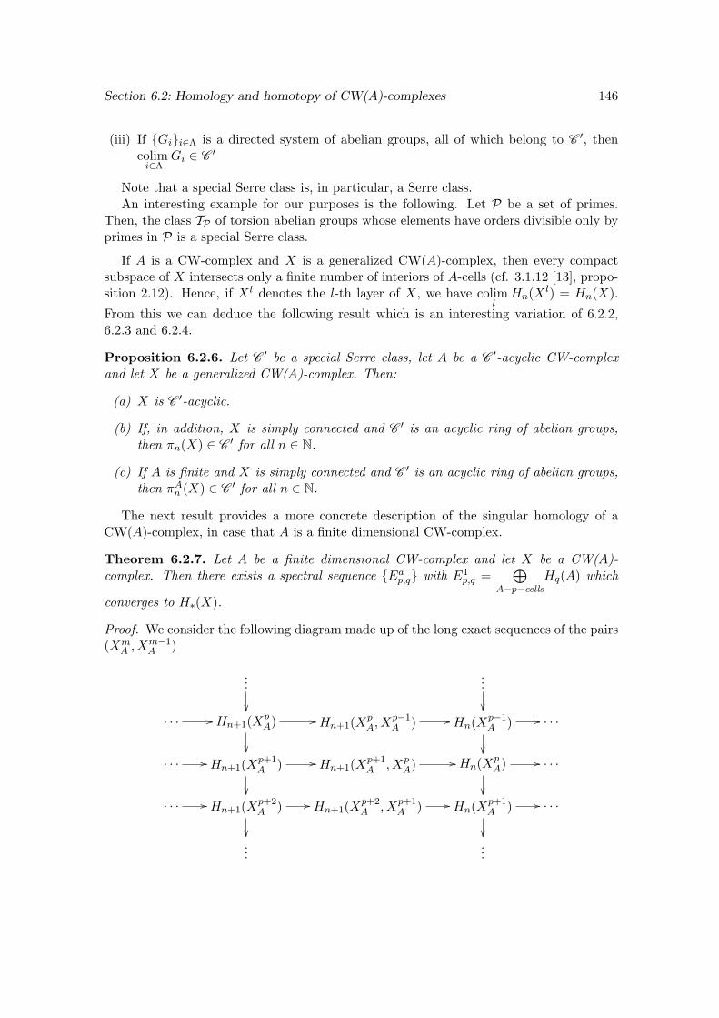
Section 6.2: Homology and homotopy of CW(A)-complexes 146
(iii) If Gii∈Λ is a directed system of abelian groups, all of which belong to C ′, thencolimi∈Λ
Gi ∈ C ′
Note that a special Serre class is, in particular, a Serre class.An interesting example for our purposes is the following. Let P be a set of primes.
Then, the class TP of torsion abelian groups whose elements have orders divisible only byprimes in P is a special Serre class.
If A is a CW-complex and X is a generalized CW(A)-complex, then every compactsubspace of X intersects only a finite number of interiors of A-cells (cf. 3.1.12 [13], propo-sition 2.12). Hence, if X l denotes the l-th layer of X, we have colim
lHn(X l) = Hn(X).
From this we can deduce the following result which is an interesting variation of 6.2.2,6.2.3 and 6.2.4.
Proposition 6.2.6. Let C ′ be a special Serre class, let A be a C ′-acyclic CW-complexand let X be a generalized CW(A)-complex. Then:
(a) X is C ′-acyclic.
(b) If, in addition, X is simply connected and C ′ is an acyclic ring of abelian groups,then πn(X) ∈ C ′ for all n ∈ N.
(c) If A is finite and X is simply connected and C ′ is an acyclic ring of abelian groups,then πAn (X) ∈ C ′ for all n ∈ N.
The next result provides a more concrete description of the singular homology of aCW(A)-complex, in case that A is a finite dimensional CW-complex.
Theorem 6.2.7. Let A be a finite dimensional CW-complex and let X be a CW(A)-complex. Then there exists a spectral sequence Eap,q with E1
p,q =⊕
A−p−cells
Hq(A) which
converges to H∗(X).
Proof. We consider the following diagram made up of the long exact sequences of the pairs(Xm
A , Xm−1A )
...
...
. . . // Hn+1(X
pA) //
Hn+1(XpA, X
p−1A ) // Hn(X
p−1A ) //
. . .
. . . // Hn+1(Xp+1A ) //
Hn+1(Xp+1A , Xp
A) // Hn(XpA) //
. . .
. . . // Hn+1(Xp+2A ) //
Hn+1(Xp+2A , Xp+1
A ) // Hn(Xp+1A ) //
. . .
......
Section 6.2: Homology and homotopy of CW(A)-complexes 147
Let E′1n,p = Hn(XpA, X
p−1A ). Note that
E′1n,p = Hn(XpA, X
p−1A ) = Hn(X
pA/X
p−1A ) = Hn(
∨A-p-cells
ΣpA) =⊕
A-p-cells
Hn(ΣpA) =
=⊕
A-p-cells
Hn−p(A).
Since A is finite-dimensional, for each n ∈ Z the set p/E′1n,p 6= 0 is finite. It is alsoclear that Hn(X
pA) = 0 for p < 0 and Hn(X
pA) = Hn(X) if p > n. Finally, we make a
change of indexes and take E1p,q = E′1p+q,p.
With a similar proof we deduce the following.
Proposition 6.2.8. If A is a Moore space of type (G,n) and X is a CW(A)-complex,then H∗(X) can be computed as the homology of a chain complex, which turns out to bethe one described in theorem 5.2.1.
Remark 6.2.9. The previous proposition generalizes theorem 5.2.1. However, the proofgiven there also gives a concise description of the differentials of the chain complex.
The following theorem generalizes theorem 6.2.7 of above and its proof is formallyidentical.
Theorem 6.2.10. Let A and B be CW-complexes, with A finite and B such that Hr(B) 6=0 only for a finite number of r’s (this holds, for example, if B is finite dimensional).Let X be a CW(B)-complex. Then there exists a spectral sequence Eap,q with E1
p,q =⊕A−p−cells
HAp+q(Σ
pB) which converges to HA∗ (X).
It is well known that if a CW-complex does not have cells of a certain dimension j, thenits j-th homology group vanishes. The following proposition heads towards that direction,giving, in several cases, a range of dimensions outside of which the A-homology groupsare trivial.
Proposition 6.2.11. Let A be an l-connected CW-complex of dimension k and let X bea topological space such that SP (X) is abelian (this holds, for example, if H1(X) = 0).
(a) If X is an abelian CW-complex of dimension m, then HAr (X) = 0 for r ≥ m− l.
(b) If X is an abelian CW(A)-complex of dimension m, then HAr (X) = 0 for
r ≥ m+ k − l.
(c) If X is an abelian CW(A)-complex without cells of dimension less than m′, thenHAr (X) = 0 for r ≤ m′ + l − k.
The proof follows immediately from the Federer spectral sequence applied to the spaceSP (X).
Section 6.3: Examples on real projective spaces 148
6.3 Examples on real projective spaces
We exhibit now some examples concerning real projective spaces.It follows from 2.5.5 that if X is a path-connected abelian topological space, every
element in πP2
n (X) (n ≥ 1) has order 1, 2 or 4. This can be generalized to Pl (for anydimension l) in the following way. By 2.5.4 we know that there is a spectral sequenceEap,q which converges to πPl
p+q(X) for p + q ≥ 1. If l is even then, for p + q ≥ 1 andp ≤ −1, we get
E2p,q ' H−p(Pl;πq(X)) =
πq(X)/2πq(X) if p is even and −p ≤ lα ∈ πq(X)/ ord (α) = 1 or 2 if p is odd and −p ≤ l
It follows that if β ∈ πPl
n (X) (and n ≥ 1) then ord (β)|2l.It is worth mentioning that if the homotopy groups of X are finite and do not contain
elements of order 2, then H−p(Pl;πq(X)) = 0 for p+ q ≥ 1 and p ≤ −1. Thus, πPl
n (X) = 0for n ≥ 1.
On the other hand, if l is odd then, for p+ q ≥ 1 and p ≤ −1, we get
E2p,q ' H−p(Pl;πq(X)) =
πq(X)/2πq(X) if p is even and −p ≤ l − 1α ∈ πq(X)/ ord (α) = 1 or 2 if p is odd and −p ≤ l − 1πq(X) if p = −l
It follows that, for n ≥ 1, there exists a short exact sequence of groups
0 // πn+l(X) // πPl
n (X) // G // 0
where G is such that exp(G)|2l−1. Note that G turns out to be solvable if n = 1, andabelian for n ≥ 2.
Now, we turn our attention to P2-homology. From example 6.1.6 we get
HP2
r (ΣP2) = H2−r(P2,Z2) =
Z2 if r = 10 if r ≥ 2
Also, from example 6.1.7 it follows that if X is a (path-connected) CW-complex, thenevery element in HP2
n (X) (n ≥ 1) has order 1, 2 or 4.
From 6.2.6 we deduce the following relationship with Eilenberg-MacLane spaces.
Example 6.3.1. There is no generalized CW(P2)-complex X such that X is a K(Z, n)for some n ≥ 2.
Example 6.3.2. For n ≥ 2, there does not exist any CW(P2)-complex which is aK(Z4, n).Indeed, if X is a CW(P2)-complex and a K(Z4, n) then by Hurewicz, Hn(X) = Z4. Butby 5.2.1 Hn(X) must be a subquotient of
⊕Z2, which entails a contradiction.
Given n ≥ 2, we construct now a generalized CW(P2)-complex which is a K(Z2, n).We need first the following lemma.
Lemma 6.3.3. Let f : S1 → X be a continuous map. Then [f ]2 = 0 in π1(X) if and onlyif f can be extended to P2.
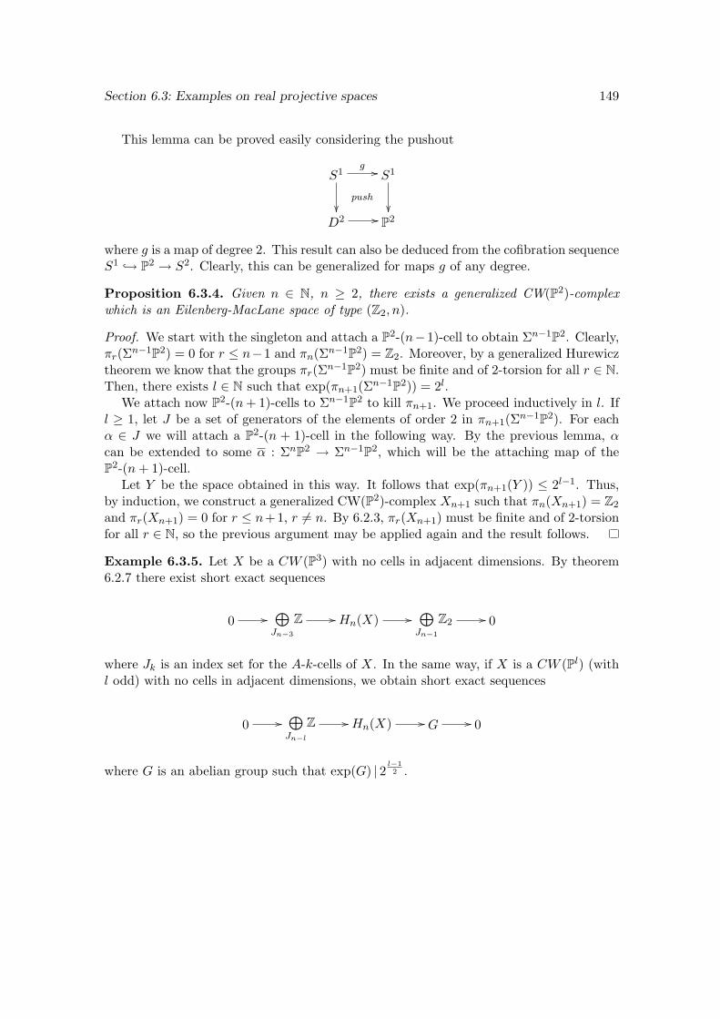
Section 6.3: Examples on real projective spaces 149
This lemma can be proved easily considering the pushout
S1g //
push
S1
D2 // P2
where g is a map of degree 2. This result can also be deduced from the cofibration sequenceS1 → P2 → S2. Clearly, this can be generalized for maps g of any degree.
Proposition 6.3.4. Given n ∈ N, n ≥ 2, there exists a generalized CW(P2)-complexwhich is an Eilenberg-MacLane space of type (Z2, n).
Proof. We start with the singleton and attach a P2-(n−1)-cell to obtain Σn−1P2. Clearly,πr(Σn−1P2) = 0 for r ≤ n−1 and πn(Σn−1P2) = Z2. Moreover, by a generalized Hurewicztheorem we know that the groups πr(Σn−1P2) must be finite and of 2-torsion for all r ∈ N.Then, there exists l ∈ N such that exp(πn+1(Σn−1P2)) = 2l.
We attach now P2-(n+ 1)-cells to Σn−1P2 to kill πn+1. We proceed inductively in l. Ifl ≥ 1, let J be a set of generators of the elements of order 2 in πn+1(Σn−1P2). For eachα ∈ J we will attach a P2-(n + 1)-cell in the following way. By the previous lemma, αcan be extended to some α : ΣnP2 → Σn−1P2, which will be the attaching map of theP2-(n+ 1)-cell.
Let Y be the space obtained in this way. It follows that exp(πn+1(Y )) ≤ 2l−1. Thus,by induction, we construct a generalized CW(P2)-complex Xn+1 such that πn(Xn+1) = Z2
and πr(Xn+1) = 0 for r ≤ n+1, r 6= n. By 6.2.3, πr(Xn+1) must be finite and of 2-torsionfor all r ∈ N, so the previous argument may be applied again and the result follows.
Example 6.3.5. Let X be a CW (P3) with no cells in adjacent dimensions. By theorem6.2.7 there exist short exact sequences
0 //⊕Jn−3
Z // Hn(X) //⊕Jn−1
Z2 // 0
where Jk is an index set for the A-k-cells of X. In the same way, if X is a CW (Pl) (withl odd) with no cells in adjacent dimensions, we obtain short exact sequences
0 //⊕Jn−l
Z // Hn(X) // G // 0
where G is an abelian group such that exp(G) | 2l−12 .
Chapter 7
CW(A)-approximations when A isa Moore space
In this chapter we give CW(A)-approximation theorems for topological spaces in case Ais a Moore space. As corollaries, we obtain homotopy classification theorems for CW(A)-complexes.
7.1 First case: A is a M(Zp, r) with p prime
Proposition 7.1.1. Let A be a Moore space of type (Zp, r) with p prime, and let Xbe a simply-connected topological space. Then there exists a CW(A)-complex Z and aweak equivalence f : Z → X if and only if Hi(X) = 0 for 1 ≤ i ≤ maxr − 1, 1 andHi(X) =
⊕Ji
Zp for all i ≥ maxr, 2.
Proof. Suppose first that there exists a CW(A)-complex Z and a weak equivalence f :Z → X. By 5.2.1 we know that, for all n ∈ N, Hn(Z) is a subquotient of
⊕A-(n− 1)-cells
Zp,
hence it is isomorphic to⊕Jn
Zp for some index set Jn. Note that Z is (r− 1)-connected by
4.1.9. Since f is a weak equivalence, it induces isomorphisms in all homology groups. ThusHi(X) = 0 for 1 ≤ i ≤ maxr − 1, 1 and Hi(X) = Hi(Z) =
⊕Ji
Zp for all i ≥ maxr, 2.
For the converse we will analize first the case r = 1 for simplicity. So, suppose thatHi(X) = 0 for 1 ≤ i ≤ 1 and Hi(X) =
⊕Ji
Zp for all i ≥ 2. Let ϕ : X ′ → X be a CW-
approximation of X. Since∨Ji
ΣiA is a Moore space of type (⊕Ji
Zp, i + 1), we may take a
homology decomposition f ′ : Z → X ′ of X ′ such that Z = colimn∈N
Zn, with Z1 = ∗ and Zn
the mapping cone of a map∨Jn
Σn−2A → Zn−1 for n ≥ 2. Hence, Z is a CW(A)-complex
and f = ϕ f ′ : Z → X is a weak equivalence.Now we study the case r ≥ 2, which is similar to the previous one. Suppose that
Hi(X) = 0 for 1 ≤ i ≤ r − 1 and Hi(X) =⊕Ji
Zp for all i ≥ r. Let ϕ : X ′ → X be a
150
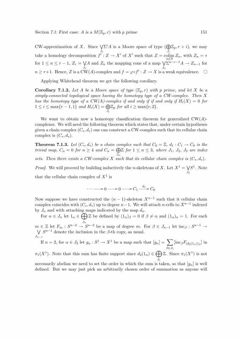
Section 7.1: First case: A is a M(Zp, r) with p prime 151
CW-approximation of X. Since∨Ji
ΣiA is a Moore space of type (⊕Ji
Zp, r + i), we may
take a homology decomposition f ′ : Z → X ′ of X ′ such that Z = colimn∈N
Zn, with Zn = ∗
for 1 ≤ n ≤ r − 1, Zr =∨Jr
A and Zn the mapping cone of a map∨Jn
Σn−r−1A → Zn−1 for
n ≥ r+1. Hence, Z is a CW(A)-complex and f = ϕf ′ : Z → X is a weak equivalence.
Applying Whitehead theorem we get the following corollary.
Corollary 7.1.2. Let A be a Moore space of type (Zp, r) with p prime, and let X be asimply-connected topological space having the homotopy type of a CW-complex. Then Xhas the homotopy type of a CW(A)-complex if and only if if and only if Hi(X) = 0 for1 ≤ i ≤ maxr − 1, 1 and Hi(X) =
⊕Ji
Zp for all i ≥ maxr, 2.
We want to obtain now a homotopy classification theorem for generalized CW(A)-complexes. We will need the following theorem which states that, under certain hypothesesgiven a chain complex (C∗, d∗) one can construct a CW-complex such that its cellular chaincomplex is (C∗, d∗).
Theorem 7.1.3. Let (C∗, d∗) be a chain complex such that C0 = Z, d1 : C1 → C0 is thetrivial map, Cn = 0 for n ≥ 4 and Cn =
⊕Jn
Z for 1 ≤ n ≤ 3, where J1, J2, J3 are index
sets. Then there exists a CW-complex X such that its cellular chain complex is (C∗, d∗).
Proof. We will proceed by building inductively the n-skeletons of X. Let X1 =∨J1
S1. Note
that the cellular chain complex of X1 is
. . . // 0 // 0 // C1d1 // C0
Now suppose we have constructed the (n − 1)-skeleton Xn−1 such that it cellular chaincomplex coincides with (C∗, d∗) up to degree n−1. We will attach n-cells to Xn−1 indexedby Jn and with attaching maps indicated by the map dn.
For α ∈ Jn let 1α ∈⊕Jn
Z be defined by (1α)β = 0 if β 6= α and (1α)α = 1. For each
m ∈ Z let Fm : Sn−2 → Sn−2 be a map of degree m. For β ∈ Jn−1 let incβ : Sn−1 →∨Jn−1
Sn−1 denote the inclusion in the β-th copy, as usual.
If n = 2, for α ∈ J2 let gα : S1 → X1 be a map such that [gα] =∑β∈J1
[incβF(d2(1α))β] in
π1(X1). Note that this sum has finite support since d2(1α) ∈⊕J1
Z. Since π1(X1) is not
necessarily abelian we need to set the order in which the sum is taken, so that [gα] is welldefined. But we may just pick an arbitrarily chosen order of summation as anyone will
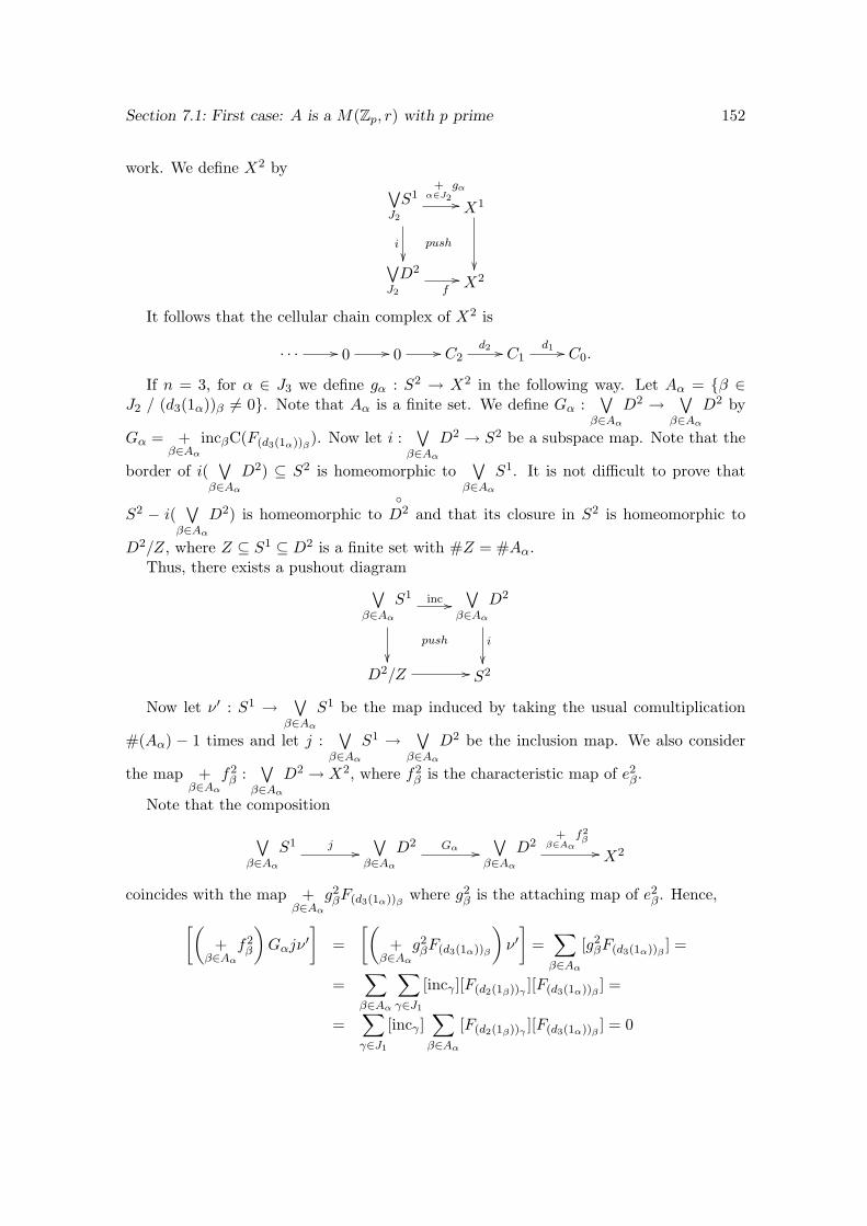
Section 7.1: First case: A is a M(Zp, r) with p prime 152
work. We define X2 by ∨J2
S1+
α∈J2
gα
//
i
push
X1
∨J2
D2
f// X2
It follows that the cellular chain complex of X2 is
. . . // 0 // 0 // C2d2 // C1
d1 // C0.
If n = 3, for α ∈ J3 we define gα : S2 → X2 in the following way. Let Aα = β ∈J2 / (d3(1α))β 6= 0. Note that Aα is a finite set. We define Gα :
∨β∈Aα
D2 →∨
β∈Aα
D2 by
Gα = +β∈Aα
incβC(F(d3(1α))β). Now let i :
∨β∈Aα
D2 → S2 be a subspace map. Note that the
border of i(∨
β∈Aα
D2) ⊆ S2 is homeomorphic to∨
β∈Aα
S1. It is not difficult to prove that
S2 − i(∨
β∈Aα
D2) is homeomorphic toD2 and that its closure in S2 is homeomorphic to
D2/Z, where Z ⊆ S1 ⊆ D2 is a finite set with #Z = #Aα.Thus, there exists a pushout diagram∨
β∈Aα
S1 inc //
push
∨β∈Aα
D2
i
D2/Z // S2
Now let ν ′ : S1 →∨
β∈Aα
S1 be the map induced by taking the usual comultiplication
#(Aα) − 1 times and let j :∨
β∈Aα
S1 →∨
β∈Aα
D2 be the inclusion map. We also consider
the map +β∈Aα
f2β :
∨β∈Aα
D2 → X2, where f2β is the characteristic map of e2β.
Note that the composition
∨β∈Aα
S1 j //∨
β∈Aα
D2 Gα //∨
β∈Aα
D2+
β∈Aαf2
β
// X2
coincides with the map +β∈Aα
g2βF(d3(1α))β
where g2β is the attaching map of e2β. Hence,[(
+β∈Aα
f2β
)Gαjν
′]
=[(
+β∈Aα
g2βF(d3(1α))β
)ν ′]
=∑β∈Aα
[g2βF(d3(1α))β
] =
=∑β∈Aα
∑γ∈J1
[incγ ][F(d2(1β))γ][F(d3(1α))β
] =
=∑γ∈J1
[incγ ]∑β∈Aα
[F(d2(1β))γ][F(d3(1α))β
] = 0
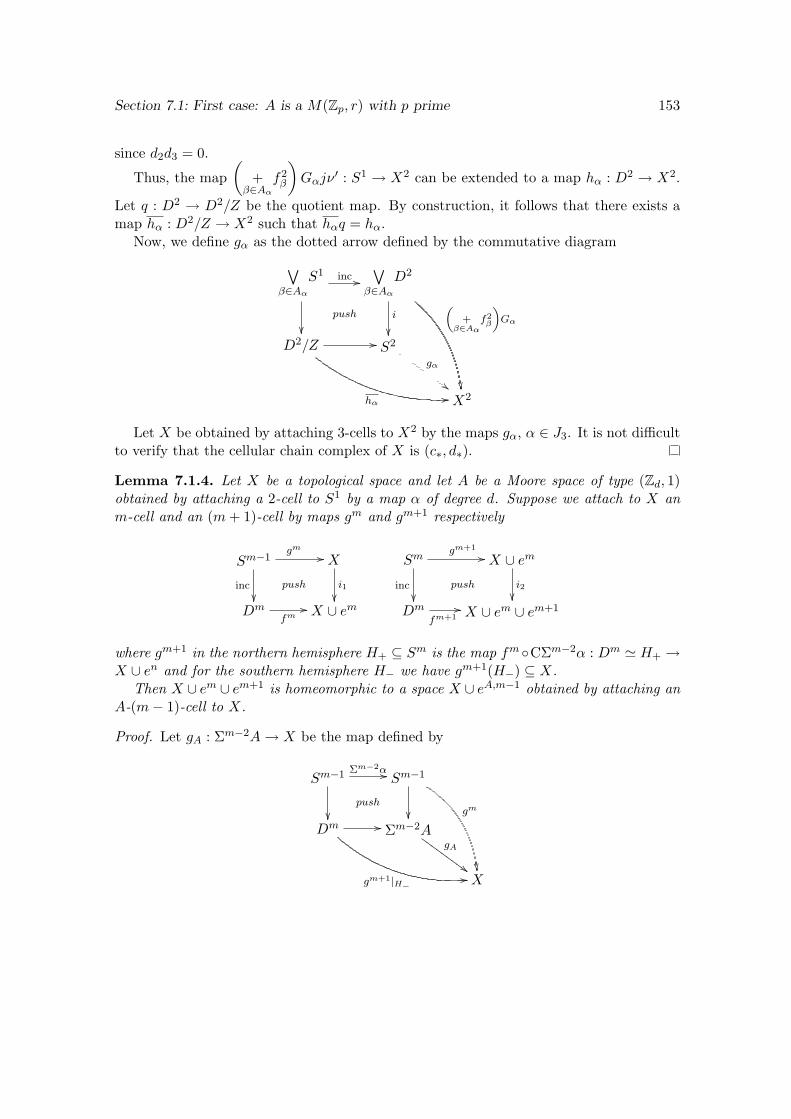
Section 7.1: First case: A is a M(Zp, r) with p prime 153
since d2d3 = 0.
Thus, the map(
+β∈Aα
f2β
)Gαjν
′ : S1 → X2 can be extended to a map hα : D2 → X2.
Let q : D2 → D2/Z be the quotient map. By construction, it follows that there exists amap hα : D2/Z → X2 such that hαq = hα.
Now, we define gα as the dotted arrow defined by the commutative diagram∨β∈Aα
S1 inc //
push
∨β∈Aα
D2
i
„+
β∈Aαf2
β
«Gα
D2/Z //
hα00
S2
gα
##X2
Let X be obtained by attaching 3-cells to X2 by the maps gα, α ∈ J3. It is not difficultto verify that the cellular chain complex of X is (c∗, d∗).
Lemma 7.1.4. Let X be a topological space and let A be a Moore space of type (Zd, 1)obtained by attaching a 2-cell to S1 by a map α of degree d. Suppose we attach to X anm-cell and an (m+ 1)-cell by maps gm and gm+1 respectively
Sm−1gm
//
inc
push
X
i1
Dmfm
// X ∪ em
Smgm+1
//
inc
push
X ∪ em
i2
Dmfm+1
// X ∪ em ∪ em+1
where gm+1 in the northern hemisphere H+ ⊆ Sm is the map fm CΣm−2α : Dm ' H+ →X ∪ en and for the southern hemisphere H− we have gm+1(H−) ⊆ X.
Then X ∪ em ∪ em+1 is homeomorphic to a space X ∪ eA,m−1 obtained by attaching anA-(m− 1)-cell to X.
Proof. Let gA : Σm−2A→ X be the map defined by
Sm−1 Σm−2α //
push
Sm−1
gm
Dm //
gm+1|H−00
Σm−2AgA
##HHHHHHHHH
X
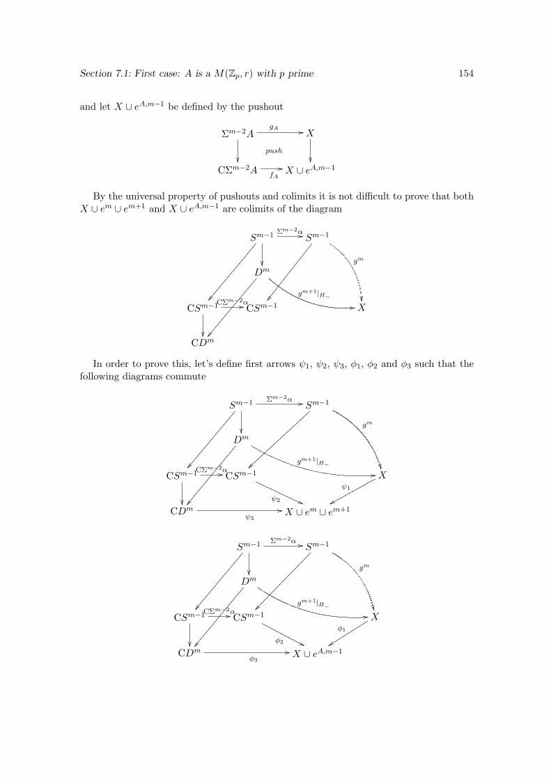
Section 7.1: First case: A is a M(Zp, r) with p prime 154
and let X ∪ eA,m−1 be defined by the pushout
Σm−2AgA //
push
X
CΣm−2A fA
// X ∪ eA,m−1
By the universal property of pushouts and colimits it is not difficult to prove that bothX ∪ em ∪ em+1 and X ∪ eA,m−1 are colimits of the diagram
Sm−1 Σm−2α//
Sm−1
gm
Dm
gm+1|H−00CSm−1CΣm−2α//
CSm−1 X
CDm
In order to prove this, let’s define first arrows ψ1, ψ2, ψ3, φ1, φ2 and φ3 such that thefollowing diagrams commute
Sm−1 Σm−2α //
Sm−1
gm
~~
Dm
gm+1|H−00CSm−1CΣm−2α//
CSm−1
ψ2 ''PPPPPPPPPPPP Xψ1
xxqqqqqqqqqqqq
CDmψ3
// X ∪ em ∪ em+1
Sm−1 Σm−2α //
Sm−1
gm
Dm
gm+1|H−00CSm−1CΣm−2α//
CSm−1
φ2 ''NNNNNNNNNNN Xφ1
yyssssssssss
CDmφ3
// X ∪ eA,m−1
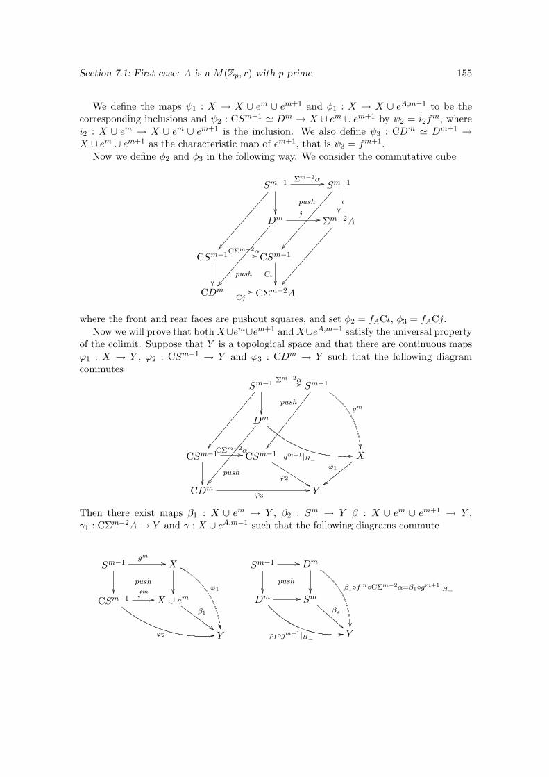
Section 7.1: First case: A is a M(Zp, r) with p prime 155
We define the maps ψ1 : X → X ∪ em ∪ em+1 and φ1 : X → X ∪ eA,m−1 to be thecorresponding inclusions and ψ2 : CSm−1 ' Dm → X ∪ em ∪ em+1 by ψ2 = i2f
m, wherei2 : X ∪ em → X ∪ em ∪ em+1 is the inclusion. We also define ψ3 : CDm ' Dm+1 →X ∪ em ∪ em+1 as the characteristic map of em+1, that is ψ3 = fm+1.
Now we define φ2 and φ3 in the following way. We consider the commutative cube
Sm−1 Σm−2α //
push
Sm−1
ι
Dmj //
Σm−2A
CSm−1CΣm−2α//
push
CSm−1
Cι
CDmCj// CΣm−2A
where the front and rear faces are pushout squares, and set φ2 = fACι, φ3 = fACj.Now we will prove that bothX∪em∪em+1 andX∪eA,m−1 satisfy the universal property
of the colimit. Suppose that Y is a topological space and that there are continuous mapsϕ1 : X → Y , ϕ2 : CSm−1 → Y and ϕ3 : CDm → Y such that the following diagramcommutes
Sm−1 Σm−2α//
push
Sm−1
gm
Dm
gm+1|H−00CSm−1CΣm−2α//
push
CSm−1
ϕ2%%KKKKKKKKKK X
ϕ1
||yyyy
yyyy
y
CDmϕ3
// Y
Then there exist maps β1 : X ∪ em → Y , β2 : Sm → Y β : X ∪ em ∪ em+1 → Y ,γ1 : CΣm−2A→ Y and γ : X ∪ eA,m−1 such that the following diagrams commute
Sm−1gm
//
push
X
ϕ1
CSm−1fm//
ϕ2 00
X ∪ emβ1
##GGGGGGGGG
Y
Sm−1 //
push
Dm
β1fmCΣm−2α=β1gm+1|H+
Dm //
ϕ1gm+1|H−00
Sm
β2
!!CCC
CCCC
C
Y
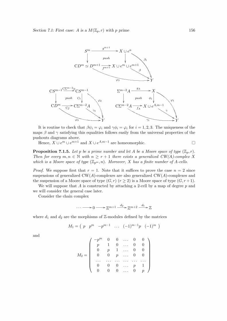
Section 7.1: First case: A is a M(Zp, r) with p prime 156
Smgm+1
//
push
X ∪ en
β1
CDm ' Dm+1fm+1
//
ϕ3 00
X ∪ em ∪ em+1
β
&&NNNNNNNNNNNN
Y
CSm−1CΣm−2α//
push
CSm−1
Cι ϕ2
CDmCj//
ϕ3 00
CΣm−2Aγ1
$$IIIII
IIIII
Y
Σm−2AgA //
push
X
φ1
ϕ1
CΣm−2A
γ1 00
fA
// X ∪ eA,m−1
γ
%%KKKKKKKKKK
Y
It is routine to check that βψi = ϕi and γφi = ϕi for i = 1, 2, 3. The uniqueness of themaps β and γ satisfying this equalities follows easily from the universal properties of thepushouts diagrams above.
Hence, X ∪ em ∪ em+1 and X ∪ eA,m−1 are homeomorphic.
Proposition 7.1.5. Let p be a prime number and let A be a Moore space of type (Zp, r).Then for every m,n ∈ N with n ≥ r + 1 there exists a generalized CW(A)-complex Xwhich is a Moore space of type (Zpm , n). Moreover, X has a finite number of A-cells.
Proof. We suppose first that r = 1. Note that it suffices to prove the case n = 2 sincesuspensions of generalized CW(A)-complexes are also generalized CW(A)-complexes andthe suspension of a Moore space of type (G, r) (r ≥ 2) is a Moore space of type (G, r+1).
We will suppose that A is constructed by attaching a 2-cell by a map of degree p andwe will consider the general case later.
Consider the chain complex
. . . // 0 // Zm+1d2 // Zm+2
d1 // Z
where d1 and d2 are the morphisms of Z-modules defined by the matrices
M1 =(p pm −pm−1 . . . (−1)m−1p (−1)m
)and
M2 =
−pm 0 0 . . . 0 0p 1 0 . . . 0 00 p 1 . . . 0 00 0 p . . . 0 0. . . . . . . . . . . . . . . . . .0 0 0 . . . p 10 0 0 . . . 0 p
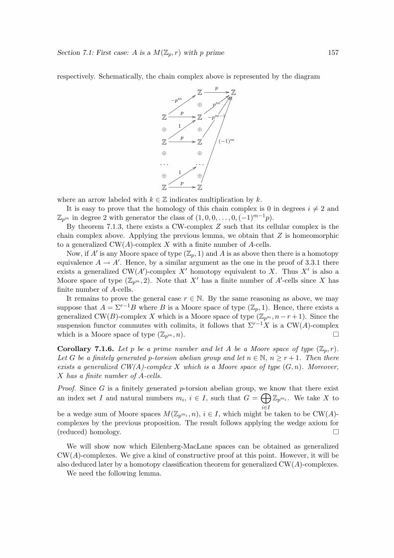
Section 7.1: First case: A is a M(Zp, r) with p prime 157
respectively. Schematically, the chain complex above is represented by the diagram
Zp //
⊕
Z
Zp //
−pm::uuuuuuuuuu
⊕
Z
pmwwww
;;wwww
⊕
Zp //
1
::uuuuuuuuuu
⊕
Z
−pm−1
DD
⊕
. . .
⊕
. . .
⊕
Zp //
1
99ssssssssssZ
(−1)m
II
where an arrow labeled with k ∈ Z indicates multiplication by k.It is easy to prove that the homology of this chain complex is 0 in degrees i 6= 2 and
Zpm in degree 2 with generator the class of (1, 0, 0, . . . , 0, (−1)m−1p).By theorem 7.1.3, there exists a CW-complex Z such that its cellular complex is the
chain complex above. Applying the previous lemma, we obtain that Z is homeomorphicto a generalized CW(A)-complex X with a finite number of A-cells.
Now, if A′ is any Moore space of type (Zp, 1) and A is as above then there is a homotopyequivalence A → A′. Hence, by a similar argument as the one in the proof of 3.3.1 thereexists a generalized CW(A′)-complex X ′ homotopy equivalent to X. Thus X ′ is also aMoore space of type (Zpm , 2). Note that X ′ has a finite number of A′-cells since X hasfinite number of A-cells.
It remains to prove the general case r ∈ N. By the same reasoning as above, we maysuppose that A = Σr−1B where B is a Moore space of type (Zp, 1). Hence, there exists ageneralized CW(B)-complex X which is a Moore space of type (Zpm , n− r+1). Since thesuspension functor commutes with colimits, it follows that Σr−1X is a CW(A)-complexwhich is a Moore space of type (Zpm , n).
Corollary 7.1.6. Let p be a prime number and let A be a Moore space of type (Zp, r).Let G be a finitely generated p-torsion abelian group and let n ∈ N, n ≥ r+ 1. Then thereexists a generalized CW(A)-complex X which is a Moore space of type (G,n). Moreover,X has a finite number of A-cells.
Proof. Since G is a finitely generated p-torsion abelian group, we know that there existan index set I and natural numbers mi, i ∈ I, such that G =
⊕i∈I
Zpmi . We take X to
be a wedge sum of Moore spaces M(Zpmi , n), i ∈ I, which might be taken to be CW(A)-complexes by the previous proposition. The result follows applying the wedge axiom for(reduced) homology.
We will show now which Eilenberg-MacLane spaces can be obtained as generalizedCW(A)-complexes. We give a kind of constructive proof at this point. However, it will bealso deduced later by a homotopy classification theorem for generalized CW(A)-complexes.
We need the following lemma.
Section 7.1: First case: A is a M(Zp, r) with p prime 158
Lemma 7.1.7. Let m ∈ N and let A be the Moore space of type (Zm, 1) obtained byattaching a 2-cell to S1 by a map g of degree m. Let f : S1 → X be a continuous map.Then [f ]m = 0 in π1(X) if and only if f can be extended to A.
Proof. Note that [f ]m = [gf ] in π1(X). Hence if [f ]m = 0 then fg ' 0 and thus it canbe extended to D2. The extension of f to A is obtained then by the universal property ofpushouts.
To prove the converse, let g : D2 → A be the characteristic map of the 2-cell of Aand let inc : S1 → D2 be the inclusion map. If f can be extended to f : A → X thengf = fginc is nullhomotopic. Hence [f ]m = [gf ] = 0.
Note that this result can also be deduced from the cofibration sequence S1 → A→ S2.
Proposition 7.1.8. Let p be a prime number and let A be a Moore space of type (Zp, r).Let G be a finitely generated p-torsion abelian group and let n ∈ N with n ≥ r + 1. Thenthere exists a generalized CW(A)-complex X which is an Eilenberg-MacLane space of type(G,n).
Proof. Applying the same argument as in the proof of 7.1.5, we may suppose that A isobtained by attaching a 2-cell to S1 by a map of degree p.
We will prove only the case r = 1, since the general case is completely analogous to it.By the previous corollary we may build a finite generalized CW(A)-complex X0 which
is also a Moore space of type (G,n). By the Hurewicz theorem, πr(X0) = 0 for r ≤ n− 1and πn(X0) = G. Moreover, by the generalized Hurewicz theorem (2.3.13) we know thatthe groups πr(X0) must be finite and of p-torsion for all r ∈ N. Then, there exists l ∈ Nsuch that exp(πn+1(X0)) = pl.
We attach now A-(n+1)-cells to X0 to kill πn+1. We proceed inductively in l. If l ≥ 1,let J be a set of generators of the elements of order p in πn+1(X0). For each α ∈ J wewill attach an A-(n+ 1)-cell in the following way. By lemma 7.1.7, α can be extended tosome α : ΣnA→ X0, which will be the attaching map of the A-(n+ 1)-cell.
Let Y be the space obtained in this way. It follows that exp(πn+1(Y )) ≤ pl−1. Thus,by induction, we may construct a finite generalized CW(A)-complex Xn+1 such thatπn(Xn+1) = Zp and πr(Xn+1) = 0 for r ≤ n + 1, r 6= n. By 6.2.3, πr(Xn+1) mustbe finite and of p-torsion for all r ∈ N, so the previous argument may be applied againand the result follows.
Theorem 7.1.9. Let p be a prime number and let A be a Moore space of type (Zp, r). LetX be an r-connected CW-complex such that Hn(X) is a finitely generated p-torsion abeliangroup for all n ≥ r+ 1. Then X has the homotopy type of a generalized CW(A)-complex.
Proof. As in the proofs above, we will only analize the case r = 1 since the general case isvery similar to that.
By 1.4.39 we know that X admits a homology decomposition. Then, there exist a CW-complex Z, a homotopy equivalence f : Z → X, and a sequence (Zn)n∈N of subcomplexesof Z such that
(a) Zn ⊆ Zn+1 for all n ∈ N.
Section 7.2: General case: A is a M(Zm, r) 159
(b) Z =⋃n∈N
Zn.
(c) Z1 is a Moore space of type (H1(X), 1).
(d) For all n ∈ N, Zn+1 is the mapping cone of a cellular map gn : Mn → Zn, whereMn is a Moore space of type (Hn+1(X), n), and gn is such that the induced map(gn)∗ : Hn(Mn) → Hn(Zn) is trivial.
Now, by 7.1.6 we may suppose that Mn is a finite generalized CW(A)-complex for alln ∈ N. By a similar argument as that of the proof of 3.1.26 it follows that Z is ageneralized CW(A)-complex.
Note that if A is a Moore space of type (Zp, r) and X is an r-connected CW-complexwhich has the homotopy type of a generalized CW(A)-complex, then by 6.2.6, Hn(X) isa p-torsion abelian group for all n ≥ r + 1. Hence, we obtain a kind of converse of theprevious theorem.
7.2 General case: A is a M(Zm, r)
To study the case where A is a Moore space of type (Zm, n), with m not necessarily prime,we will make use of the following theorem, due to J.H.C. Whitehead [23].
Theorem 7.2.1. Let (C∗, d∗) be a chain complex such that C0 = Z, C1 = 0 and Cn =⊕Jn
Z
for each n ≥ 2, where Jn, n ≥ 2, are index sets. Then there exists a simply-connectedCW-complex X such that its cellular chain complex is (C∗, d∗).
Proof. For each n ∈ N, we will construct a CW-complex Xn of dimension n with cellularchain complex (C(n)
∗ , d(n)∗ ) such that
• (Xn)n−1 = Xn−1
• C(n)i = Ci if 0 ≤ i ≤ n
• C(n)i = 0 if i > n
• d(n)i = di if 1 ≤ i ≤ n
• d(n)i = 0 if i > n or i = 1
• If jn : πn(Xn) → πn(Xn, Xn−1) and ∂n : πn(Xn, Xn−1) → πn−1(Xn−1) are mor-phisms coming from the long exact sequence of homotopy groups associated to thepair (Xn, Xn−1), then Im jn = ker(jn−1∂n).
We proceed by induction on n. For n = 1 we take X1 = ∗ and for n = 2 we takeX2 =
∨J2
S2. From the long exact sequence of homotopy groups associated to the pair
(X2, X1) it follows that Im j2 = π2(X2, X1) which coincides with ker(j1∂2), since j1∂2 isthe trivial map.
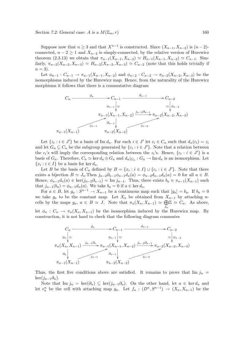
Section 7.2: General case: A is a M(Zm, r) 160
Suppose now that n ≥ 3 and that Xn−1 is constructed. Since (Xn−1, Xn−2) is (n− 2)-connected, n − 2 ≥ 1 and Xn−2 is simply-connected, by the relative version of Hurewicztheorem (2.3.13) we obtain that πn−1(Xn−1, Xn−2) ' Hn−1(Xn−1, Xn−2) ' Cn−1. Sim-ilarly, πn−2(Xn−2, Xn−3) ' Hn−2(Xn−2, Xn−3) ' Cn−2 (note that this holds trivially ifn = 3).
Let φn−1 : Cn−1 → πn−1(Xn−1, Xn−2) and φn−2 : Cn−2 → πn−2(Xn−2, Xn−3) be theisomorphisms induced by the Hurewicz map. Hence, from the naturality of the Hurewiczmorphisms it follows that there is a commutative diagram
Cndn // Cn−1
dn−1 //
φn−1 '
Cn−2
φn−2'
πn−1(Xn−1, Xn−2)jn−2∂n−1 //
∂n−1
πn−2(Xn−2, Xn−3)
πn−1(Xn−1)jn−1
55jjjjjjjjjjjjjjjπn−2(Xn−2)
jn−2
44iiiiiiiiiiiiiiiii
Let zi : i ∈ J ′ be a basis of Im dn. For each i ∈ J ′ let ci ∈ Cn such that dn(ci) = ziand let Gn ⊆ Cn be the subgroup generated by ci : i ∈ J ′. Note that a relation betweenthe ci’s will imply the corresponding relation between the zi’s. Hence, ci : i ∈ J ′ is abasis of Gn. Therefore, Cn ' ker dn⊕Gn and dn|Gn : Gn → Im dn is an isomorphism. Letxi : i ∈ I be a basis for ker dn.
Let B be the basis of Cn defined by B = xi : i ∈ I ∪ ci : i ∈ J ′. Note that thereexists a bijection B ' Jn.Then jn−2∂n−1φn−1dn(a) = φn−2dn−1dn(a) = 0 for all a ∈ B.Hence, φn−1dn(a) ∈ ker(jn−2∂n−1) = Im jn−1. Thus, there exists ba ∈ πn−1(Xn−1) suchthat jn−1(ba) = φn−1dn(a). We take ba = 0 if a ∈ ker dn.
For a ∈ B, let ga : Sn−1 → Xn−1 be a continuous map such that [ga] = ba. If ba = 0we take ga to be the constant map. Let Xn be obtained from Xn−1 by attaching n-cells by the maps ga, a ∈ B ' J . Note that πn(Xn, Xn−1) '
⊕Jn
Z ' Cn. As above,
let φn : Cn → πn(Xn, Xn−1) be the isomorphism induced by the Hurewicz map. Byconstruction, it is not hard to check that the following diagram commutes
Cndn //
φn '
Cn−1dn−1 //
φn−1 '
Cn−2
φn−2'
πn(Xn, Xn−1)jn−1∂n //
∂n
πn−1(Xn−1, Xn−2)jn−2∂n−1 //
∂n−1
πn−2(Xn−2, Xn−3)
πn−1(Xn−1)jn−1
44jjjjjjjjjjjjjjjjπn−2(Xn−2)
jn−2
44iiiiiiiiiiiiiiiii
Thus, the first five conditions above are satisfied. It remains to prove that Im jn =ker(jn−1∂n).
Note that Im jn = ker(∂n) ⊆ ker(jn−1∂n). On the other hand, let a ∈ ker dn andlet ena be the cell with attaching map ga. Let fa : (Dn, Sn−1) → (Xn, Xn−1) be the
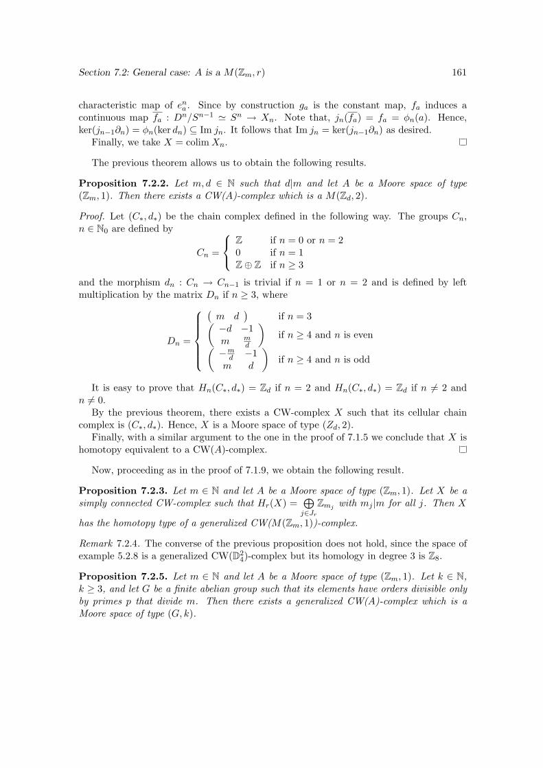
Section 7.2: General case: A is a M(Zm, r) 161
characteristic map of ena . Since by construction ga is the constant map, fa induces acontinuous map fa : Dn/Sn−1 ' Sn → Xn. Note that, jn(fa) = fa = φn(a). Hence,ker(jn−1∂n) = φn(ker dn) ⊆ Im jn. It follows that Im jn = ker(jn−1∂n) as desired.
Finally, we take X = colimXn.
The previous theorem allows us to obtain the following results.
Proposition 7.2.2. Let m, d ∈ N such that d|m and let A be a Moore space of type(Zm, 1). Then there exists a CW(A)-complex which is a M(Zd, 2).
Proof. Let (C∗, d∗) be the chain complex defined in the following way. The groups Cn,n ∈ N0 are defined by
Cn =
Z if n = 0 or n = 20 if n = 1Z⊕ Z if n ≥ 3
and the morphism dn : Cn → Cn−1 is trivial if n = 1 or n = 2 and is defined by leftmultiplication by the matrix Dn if n ≥ 3, where
Dn =
(m d
)if n = 3(
−d −1m m
d
)if n ≥ 4 and n is even(
−md −1m d
)if n ≥ 4 and n is odd
It is easy to prove that Hn(C∗, d∗) = Zd if n = 2 and Hn(C∗, d∗) = Zd if n 6= 2 andn 6= 0.
By the previous theorem, there exists a CW-complex X such that its cellular chaincomplex is (C∗, d∗). Hence, X is a Moore space of type (Zd, 2).
Finally, with a similar argument to the one in the proof of 7.1.5 we conclude that X ishomotopy equivalent to a CW(A)-complex.
Now, proceeding as in the proof of 7.1.9, we obtain the following result.
Proposition 7.2.3. Let m ∈ N and let A be a Moore space of type (Zm, 1). Let X be asimply connected CW-complex such that Hr(X) =
⊕j∈Jr
Zmj with mj |m for all j. Then X
has the homotopy type of a generalized CW(M(Zm, 1))-complex.
Remark 7.2.4. The converse of the previous proposition does not hold, since the space ofexample 5.2.8 is a generalized CW(D2
4)-complex but its homology in degree 3 is Z8.
Proposition 7.2.5. Let m ∈ N and let A be a Moore space of type (Zm, 1). Let k ∈ N,k ≥ 3, and let G be a finite abelian group such that its elements have orders divisible onlyby primes p that divide m. Then there exists a generalized CW(A)-complex which is aMoore space of type (G, k).
Section 7.2: General case: A is a M(Zm, r) 162
Proof. As in the proof of 7.1.5, it suffices to prove the case k = 3. We know that G isthe direct sum of cyclic groups of order a power of a prime that divides m. Since reducedsingular homology groups satisfy the wedge axiom, it suffices to analize the case G = Zpr ,where p|m.
By 7.2.2, there exists a CW(A)-complex B which is a Moore space of type (Zpr , 2). By7.1.5, there exists a generalized CW(B)-complex X which is a Moore space of type (G, 3).Finally, X is a CW(A)-complex by 3.1.29.
Now we obtain another homotopy classification theorem.
Theorem 7.2.6. Let m ∈ N and let A be a Moore space of type (Zm, r). Let X be a(r + 1)-connected CW-complex such that for all n ≥ r + 2, Hn(X) is a finite abeliangroup whose elements have orders divisible only by primes that divide m. Then X has thehomotopy type of a generalized CW(A)-complex.
Its proof is analogous to that of 7.1.9. Note that by 6.2.6 if an (r + 1)-connected CW-complex X has the homotopy type of a generalized CW(A)-complex then for all n ≥ r+2,Hn(X) is a torsion abelian group whose elements have orders divisible only by primes thatdivide m. Hence, we have a kind of converse of the previous theorem.
Chapter 8
Obstruction theory
In this chapter we start developing an obstruction theory for CW(A)-complexes. However,the A-cellular chain complex introduced in chapter 5 is not suitable for this purpose. Thus,we define a new A-cellular chain complex which fulfils our requirements. It is interesting topoint out that although this new chain complex is completely different from the previousone, it coincides with the classical cellular chain complex if A = S0.
We also define an obstruction cocycle and a difference cochain, which give the exactobstructions to extension problems for maps, as we shall see. These are as generalizationsof the classical ones. We emphasize that the crucial part is the definition of an adequateA-cellular chain complex so that classical obstruction theory can be taken to our moregeneral setting.
This chapter is only an introduction to obstruction theory for CW(A)-complexes. Muchmore work can be done.
8.1 A new A-cellular chain complex
Let A be an l-connected and compact CW-complex of dimension k with k ≤ 2l and l ≥ 1.By theorem 11 of [19] p. 458 the map Σ : [ΣnA,ΣnA] = πAn (A) → [Σn+1A,Σn+1A] =πAn+1(A) is a bijection for n ≥ 0 and hence an isomorphism of groups for n ≥ 1.
Let R = πA,st0 (X) = colimn
πAn (ΣnX). Then R is isomorphic to πAr (ΣrA) for r ≥ 2.
We will note by + the usual abelian group operation in πAr (ΣrA). We will also definea product in πAr (ΣrA) as follows: [f ][g] = [g f ]. It is clear that this operation is welldefined and associative and has an identity element [Id].
Also, ([f ]+ [g])[h] = h∗([f ]+ [g]) = h∗([f ])+h∗([g]) = [f ][h]+ [g][h]. We will prove nowthat [h]([f ] + [g]) = [h][f ] + [h][g]. If [h] ∈ πAr (ΣrA) by the isomorphism πAr−1(Σ
r−1A) 'πAr (ΣrA) we know that there exists [h′] ∈ πAr−1(Σ
r−1A) such that [h] = [Σh′]. We denoteby q : ΣrA→ ΣrA ∨ ΣrA the quotient map which induces the sum +. Then
[h]([f ] + [g]) = [h][(f + g) q] = [(f + g) q h] = [(f + g) q Σh′] == [(f + g) (Σh′ ∨ Σh′) q] = [(f Σh′ + g Σh′) q] == [f Σh′] + [g Σh′] = [f h] + [g h] = [h][f ] + [h][g].
Hence πAr (ΣrA) is a unital ring.
163
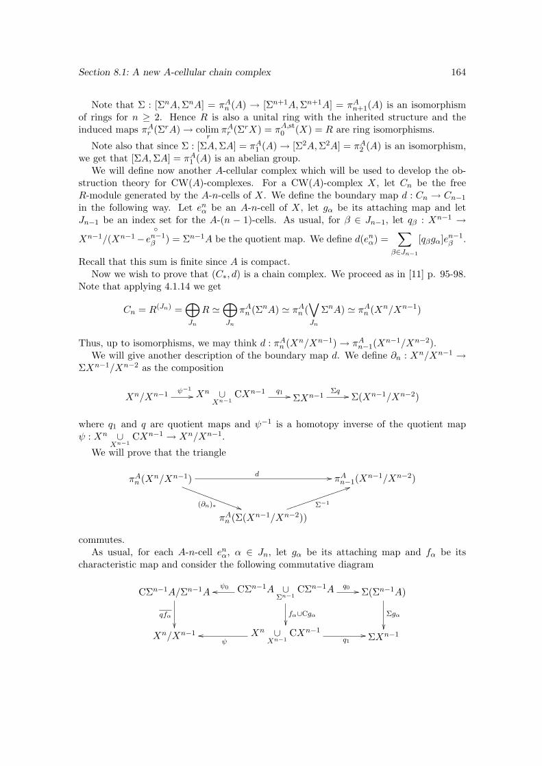
Section 8.1: A new A-cellular chain complex 164
Note that Σ : [ΣnA,ΣnA] = πAn (A) → [Σn+1A,Σn+1A] = πAn+1(A) is an isomorphismof rings for n ≥ 2. Hence R is also a unital ring with the inherited structure and theinduced maps πAr (ΣrA) → colim
rπAr (ΣrX) = πA,st0 (X) = R are ring isomorphisms.
Note also that since Σ : [ΣA,ΣA] = πA1 (A) → [Σ2A,Σ2A] = πA2 (A) is an isomorphism,we get that [ΣA,ΣA] = πA1 (A) is an abelian group.
We will define now another A-cellular complex which will be used to develop the ob-struction theory for CW(A)-complexes. For a CW(A)-complex X, let Cn be the freeR-module generated by the A-n-cells of X. We define the boundary map d : Cn → Cn−1
in the following way. Let enα be an A-n-cell of X, let gα be its attaching map and letJn−1 be an index set for the A-(n − 1)-cells. As usual, for β ∈ Jn−1, let qβ : Xn−1 →
Xn−1/(Xn−1−
en−1β ) = Σn−1A be the quotient map. We define d(enα) =
∑β∈Jn−1
[qβgα]en−1β .
Recall that this sum is finite since A is compact.Now we wish to prove that (C∗, d) is a chain complex. We proceed as in [11] p. 95-98.
Note that applying 4.1.14 we get
Cn = R(Jn) =⊕Jn
R '⊕Jn
πAn (ΣnA) ' πAn (∨Jn
ΣnA) ' πAn (Xn/Xn−1)
Thus, up to isomorphisms, we may think d : πAn (Xn/Xn−1) → πAn−1(Xn−1/Xn−2).
We will give another description of the boundary map d. We define ∂n : Xn/Xn−1 →ΣXn−1/Xn−2 as the composition
Xn/Xn−1 ψ−1// Xn ∪
Xn−1CXn−1 q1 // ΣXn−1
Σq // Σ(Xn−1/Xn−2)
where q1 and q are quotient maps and ψ−1 is a homotopy inverse of the quotient mapψ : Xn ∪
Xn−1CXn−1 → Xn/Xn−1.
We will prove that the triangle
πAn (Xn/Xn−1) d //
(∂n)∗ ))SSSSSSSSSSSSSSπAn−1(X
n−1/Xn−2)
πAn (Σ(Xn−1/Xn−2))Σ−1
55jjjjjjjjjjjjjjj
commutes.As usual, for each A-n-cell enα, α ∈ Jn, let gα be its attaching map and fα be its
characteristic map and consider the following commutative diagram
CΣn−1A/Σn−1A
qfα
CΣn−1A ∪Σn−1
CΣn−1Aψ0oo q0 //
fα∪Cgα
Σ(Σn−1A)
Σgα
Xn/Xn−1 Xn ∪
Xn−1CXn−1
ψoo
q1// ΣXn−1
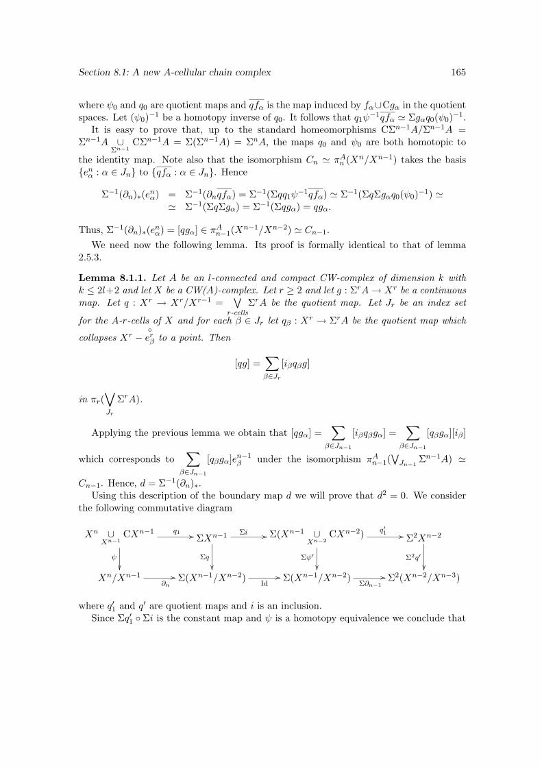
Section 8.1: A new A-cellular chain complex 165
where ψ0 and q0 are quotient maps and qfα is the map induced by fα∪Cgα in the quotientspaces. Let (ψ0)−1 be a homotopy inverse of q0. It follows that q1ψ−1qfα ' Σgαq0(ψ0)−1.
It is easy to prove that, up to the standard homeomorphisms CΣn−1A/Σn−1A =Σn−1A ∪
Σn−1CΣn−1A = Σ(Σn−1A) = ΣnA, the maps q0 and ψ0 are both homotopic to
the identity map. Note also that the isomorphism Cn ' πAn (Xn/Xn−1) takes the basisenα : α ∈ Jn to qfα : α ∈ Jn. Hence
Σ−1(∂n)∗(enα) = Σ−1(∂nqfα) = Σ−1(Σqq1ψ−1qfα) ' Σ−1(ΣqΣgαq0(ψ0)−1) '' Σ−1(ΣqΣgα) = Σ−1(Σqgα) = qgα.
Thus, Σ−1(∂n)∗(enα) = [qgα] ∈ πAn−1(Xn−1/Xn−2) ' Cn−1.
We need now the following lemma. Its proof is formally identical to that of lemma2.5.3.
Lemma 8.1.1. Let A be an l-connected and compact CW-complex of dimension k withk ≤ 2l+2 and let X be a CW(A)-complex. Let r ≥ 2 and let g : ΣrA→ Xr be a continuousmap. Let q : Xr → Xr/Xr−1 =
∨r-cells
ΣrA be the quotient map. Let Jr be an index set
for the A-r-cells of X and for each β ∈ Jr let qβ : Xr → ΣrA be the quotient map which
collapses Xr −erβ to a point. Then
[qg] =∑β∈Jr
[iβqβg]
in πr(∨Jr
ΣrA).
Applying the previous lemma we obtain that [qgα] =∑
β∈Jn−1
[iβqβgα] =∑
β∈Jn−1
[qβgα][iβ]
which corresponds to∑
β∈Jn−1
[qβgα]en−1β under the isomorphism πAn−1(
∨Jn−1
Σn−1A) '
Cn−1. Hence, d = Σ−1(∂n)∗.Using this description of the boundary map d we will prove that d2 = 0. We consider
the following commutative diagram
Xn ∪Xn−1
CXn−1 q1 //
ψ
ΣXn−1 Σi //
Σq
Σ(Xn−1 ∪Xn−2
CXn−2) q′1 //
Σψ′
Σ2Xn−2
Σ2q′
Xn/Xn−1
∂n
// Σ(Xn−1/Xn−2)Id
// Σ(Xn−1/Xn−2)Σ∂n−1
// Σ2(Xn−2/Xn−3)
where q′1 and q′ are quotient maps and i is an inclusion.Since Σq′1 Σi is the constant map and ψ is a homotopy equivalence we conclude that
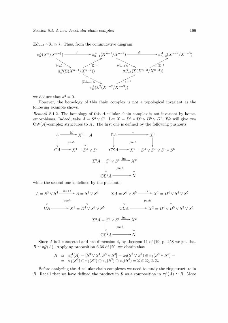
Section 8.1: A new A-cellular chain complex 166
Σ∂n−1 ∂n ' ∗. Thus, from the commutative diagram
πAn (Xn/Xn−1) d //
(∂n)∗ %%KKKKKKKKKKπAn−1(X
n−1/Xn−2) d //
(∂n−1)∗ ''PPPPPPPPPPPPπAn−2(X
n−2/Xn−3)
πAn (Σ(Xn−1/Xn−2))Σ−1
77ooooooooooo
(Σ∂n−1)∗ ''OOOOOOOOOOOπAn−1(Σ(Xn−2/Xn−3))
Σ−1
77ppppppppppp
πAn (Σ2(Xn−2/Xn−3))Σ−1
77nnnnnnnnnnnn
we deduce that d2 = 0.However, the homology of this chain complex is not a topological invariant as the
following example shows.
Remark 8.1.2. The homology of this A-cellular chain complex is not invariant by home-omorphisms. Indeed, take A = S3 ∨ S4. Let X = D4 ∨D5 ∨D6 ∨D7. We will give twoCW(A)-complex structures to X. The first one is defined by the following pushouts
AId //
push
X0 = A
CA // X1 = D4 ∨D5
ΣA∗ //
push
X1
CΣA // X2 = D4 ∨D5 ∨ S5 ∨ S6
Σ2A = S5 ∨ S6 inc //
push
X2
CΣ2A // X
while the second one is defined by the pushouts
A = S3 ∨ S4in1+∗ //
push
A = S3 ∨ S4
CA // X1 = D4 ∨ S4 ∨ S5
ΣA = S4 ∨ S5 ∗ //
push
X1 = D4 ∨ S4 ∨ S5
CΣA // X2 = D4 ∨D5 ∨ S5 ∨ S6
Σ2A = S5 ∨ S6 inc //
push
X2
CΣ2A // X
Since A is 2-connected and has dimension 4, by theorem 11 of [19] p. 458 we get thatR ' πA0 (A). Applying proposition 6.36 of [20] we obtain that
R ' πA0 (A) = [S3 ∨ S4, S3 ∨ S4] = π3(S3 ∨ S4)⊕ π4(S3 ∨ S4) == π3(S3)⊕ π3(S4)⊕ π4(S3)⊕ π4(S4) = Z⊕ Z2 ⊕ Z.
Before analyzing the A-cellular chain complexes we need to study the ring structure inR. Recall that we have defined the product in R as a composition in πA0 (A) ' R. More
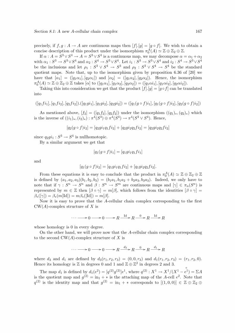
Section 8.1: A new A-cellular chain complex 167
precisely, if f, g : A → A are continuous maps then [f ].[g] = [g f ]. We wish to obtain aconcise description of this product under the isomorphism πA0 (A) ' Z⊕ Z2 ⊕ Z.
If α : A = S3∨S4 → A = S3∨S4 is a continuous map, we may decompose α = α1 +α2
with α1 : S3 → S3∨S4 and α2 : S4 → S3∨S4. Let i1 : S3 → S3∨S4 and i2 : S4 → S3∨S4
be the inclusions and let ρ1 : S3 ∨ S4 → S3 and ρ2 : S3 ∨ S4 → S4 be the standardquotient maps. Note that, up to the isomorphism given by proposition 6.36 of [20] wehave that [α1] = ([q1α1], [q2α1]) and [α2] = ([q1α2], [q2α2]). Hence, the isomorphismπA0 (A) ' Z⊕ Z2 ⊕ Z takes [α] to ([q1α1], [q1α2], [q2α2]) = ([q1αi1], [q1αi2], [q2αi2]).
Taking this into consideration we get that the product [f ].[g] = [gf ] can be translatedinto
([q1fi1], [q1fi2], [q2fi2]).([q1gi1], [q1gi2], [q2gi2]) = ([q1(g f)i1], [q1(g f)i2], [q2(g f)i2])
As mentioned above, [f2] = ([q1f2], [q2f2]) under the isomorphism ((q1)∗, (q2)∗) whichis the inverse of ((i1)∗, (i2)∗) : π4(S3)⊕ π4(S4) → π4(S3 ∨ S4). Hence,
[q2(g f)i2] = [q2gi1q1fi2] + [q2gi2q2fi2] = [q2gi2q2fi2]
since q2gi1 : S3 → S4 is nullhomotopic.By a similar argument we get that
[q1(g f)i1] = [q1gi1q1fi1]
and[q1(g f)i2] = [q1gi1q1fi2] + [q1gi2q2fi2].
From these equations it is easy to conclude that the product in πA0 (A) ' Z ⊕ Z2 ⊕ Zis defined by (a1, a2, a3)(b1, b2, b3) = (b1a1, b1a2 + b2a3, b3a3). Indeed, we only have tonote that if γ : Sn → Sn and β : Sn → Sm are continuous maps and [γ] ∈ πn(Sn) isrepresented by m ∈ Z then [β γ] = m[β], which follows from the identities [β γ] =β∗([γ]) = β∗(m[Id]) = mβ∗([Id]) = m[β].
Now it is easy to prove that the A-cellular chain complex corresponding to the firstCW(A)-complex structure of X is
. . . // 0 // 0 // RId // R
0 // RId // R
whose homology is 0 in every degree.On the other hand, we will prove now that the A-cellular chain complex corresponding
to the second CW(A)-complex structure of X is
. . . // 0 // 0 // Rd3 // R
0 // Rd1 // R
where d3 and d1 are defined by d3(r1, r2, r3) = (0, 0, r3) and d1(r1, r2, r3) = (r1, r2, 0).Hence its homology is Z in degrees 0 and 1 and Z⊕ Z2 in degrees 2 and 3.
The map d1 is defined by d1(e2) = [q(2)g(2)]e1, where q(2) : X1 → X1/(X1 −e1) = ΣA
is the quotient map and g(2) = in1 + ∗ is the attaching map of the A-cell e2. Note thatq(2) is the identity map and that g(2) = in1 + ∗ corresponds to [(1, 0, 0)] ∈ Z ⊕ Z2 ⊕
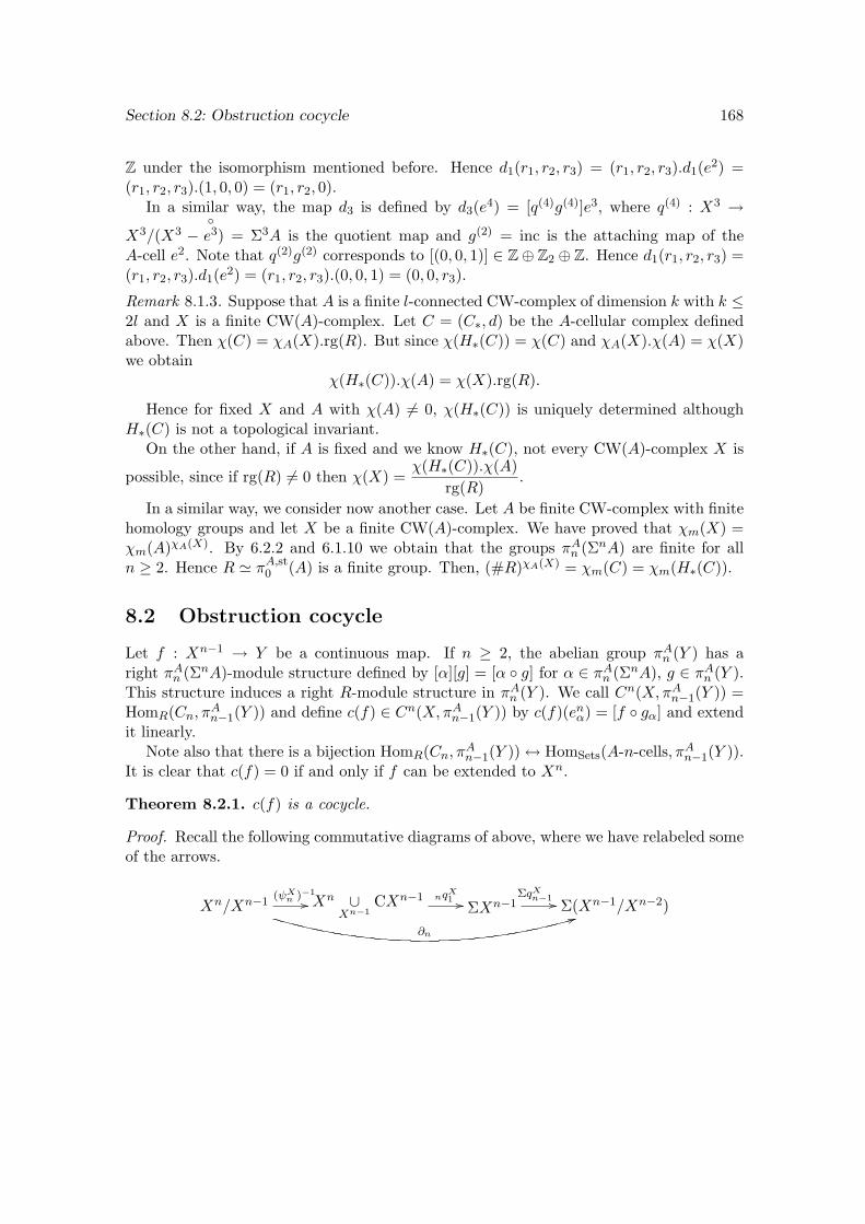
Section 8.2: Obstruction cocycle 168
Z under the isomorphism mentioned before. Hence d1(r1, r2, r3) = (r1, r2, r3).d1(e2) =(r1, r2, r3).(1, 0, 0) = (r1, r2, 0).
In a similar way, the map d3 is defined by d3(e4) = [q(4)g(4)]e3, where q(4) : X3 →
X3/(X3 −e3) = Σ3A is the quotient map and g(2) = inc is the attaching map of the
A-cell e2. Note that q(2)g(2) corresponds to [(0, 0, 1)] ∈ Z⊕ Z2 ⊕ Z. Hence d1(r1, r2, r3) =(r1, r2, r3).d1(e2) = (r1, r2, r3).(0, 0, 1) = (0, 0, r3).
Remark 8.1.3. Suppose that A is a finite l-connected CW-complex of dimension k with k ≤2l and X is a finite CW(A)-complex. Let C = (C∗, d) be the A-cellular complex definedabove. Then χ(C) = χA(X).rg(R). But since χ(H∗(C)) = χ(C) and χA(X).χ(A) = χ(X)we obtain
χ(H∗(C)).χ(A) = χ(X).rg(R).
Hence for fixed X and A with χ(A) 6= 0, χ(H∗(C)) is uniquely determined althoughH∗(C) is not a topological invariant.
On the other hand, if A is fixed and we know H∗(C), not every CW(A)-complex X is
possible, since if rg(R) 6= 0 then χ(X) =χ(H∗(C)).χ(A)
rg(R).
In a similar way, we consider now another case. Let A be finite CW-complex with finitehomology groups and let X be a finite CW(A)-complex. We have proved that χm(X) =χm(A)χA(X). By 6.2.2 and 6.1.10 we obtain that the groups πAn (ΣnA) are finite for alln ≥ 2. Hence R ' πA,st0 (A) is a finite group. Then, (#R)χA(X) = χm(C) = χm(H∗(C)).
8.2 Obstruction cocycle
Let f : Xn−1 → Y be a continuous map. If n ≥ 2, the abelian group πAn (Y ) has aright πAn (ΣnA)-module structure defined by [α][g] = [α g] for α ∈ πAn (ΣnA), g ∈ πAn (Y ).This structure induces a right R-module structure in πAn (Y ). We call Cn(X,πAn−1(Y )) =HomR(Cn, πAn−1(Y )) and define c(f) ∈ Cn(X,πAn−1(Y )) by c(f)(enα) = [f gα] and extendit linearly.
Note also that there is a bijection HomR(Cn, πAn−1(Y )) ↔ HomSets(A-n-cells, πAn−1(Y )).It is clear that c(f) = 0 if and only if f can be extended to Xn.
Theorem 8.2.1. c(f) is a cocycle.
Proof. Recall the following commutative diagrams of above, where we have relabeled someof the arrows.
Xn/Xn−1(ψX
n )−1
//
∂n
44Xn ∪
Xn−1CXn−1 nqX
1 // ΣXn−1ΣqX
n−1 // Σ(Xn−1/Xn−2)
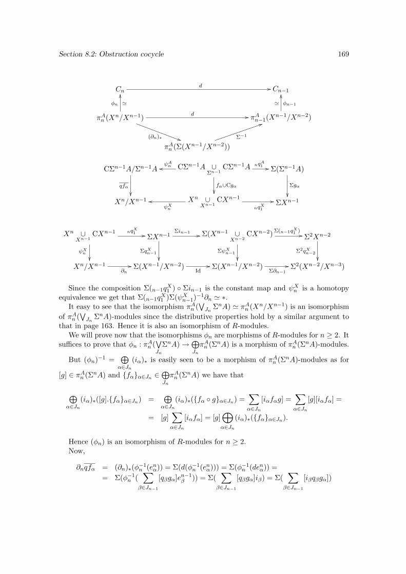
Section 8.2: Obstruction cocycle 169
Cnd // Cn−1
πAn (Xn/Xn−1) d //
(∂n)∗ ))SSSSSSSSSSSSSS
φn '
OO
πAn−1(Xn−1/Xn−2)
φn−1'
OO
πAn (Σ(Xn−1/Xn−2))Σ−1
55jjjjjjjjjjjjjjj
CΣn−1A/Σn−1A
qfα
CΣn−1A ∪Σn−1
CΣn−1AψAnoo nqA
1 //
fα∪Cgα
Σ(Σn−1A)
Σgα
Xn/Xn−1 Xn ∪
Xn−1CXn−1
ψXn
oonqX
1
// ΣXn−1
Xn ∪Xn−1
CXn−1 nqX1 //
ψXn
ΣXn−1Σin−1 //
ΣqXn−1
Σ(Xn−1 ∪Xn−2
CXn−2) Σ(n−1qX1 )//
ΣψXn−1
Σ2Xn−2
Σ2qXn−2
Xn/Xn−1
∂n
// Σ(Xn−1/Xn−2)Id
// Σ(Xn−1/Xn−2)Σ∂n−1
// Σ2(Xn−2/Xn−3)
Since the composition Σ(n−1qX1 ) Σin−1 is the constant map and ψXn is a homotopy
equivalence we get that Σ(n−1qX1 )Σ(ψXn−1)
−1∂n ' ∗.It easy to see that the isomorphism πAn (
∨Jn
ΣnA) ' πAn (Xn/Xn−1) is an isomorphismof πAn (
∨Jn
ΣnA)-modules since the distributive properties hold by a similar argument tothat in page 163. Hence it is also an isomorphism of R-modules.
We will prove now that the isomorphisms φn are morphisms of R-modules for n ≥ 2. Itsuffices to prove that φn : πAn (
∨Jn
ΣnA) →⊕Jn
πAn (ΣnA) is a morphism of πAn (ΣnA)-modules.
But (φn)−1 =⊕α∈Jn
(iα)∗ is easily seen to be a morphism of πAn (ΣnA)-modules as for
[g] ∈ πAn (ΣnA) and fαα∈Jn ∈⊕Jn
πAn (ΣnA) we have that
⊕α∈Jn
(iα)∗([g].fαα∈Jn) =⊕α∈Jn
(iα)∗(fα gα∈Jn) =∑α∈Jn
[iαfαg] =∑α∈Jn
[g][iαfα] =
= [g]∑α∈Jn
[iαfα] = [g]⊕α∈Jn
(iα)∗(fαα∈Jn).
Hence (φn) is an isomorphism of R-modules for n ≥ 2.Now,
∂nqfα = (∂n)∗(φ−1n (enα)) = Σ(d(φ−1
n (enα))) = Σ(φ−1n (denα)) =
= Σ(φ−1n (
∑β∈Jn−1
[qβgα]en−1β )) = Σ(
∑β∈Jn−1
[qβgα]iβ) = Σ(∑
β∈Jn−1
[iβqβgα])
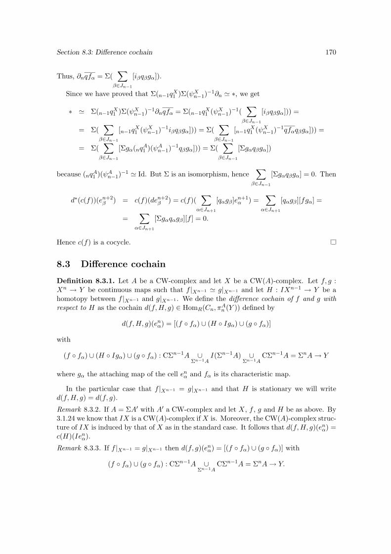
Section 8.3: Difference cochain 170
Thus, ∂nqfα = Σ(∑
β∈Jn−1
[iβqβgα]).
Since we have proved that Σ(n−1qX1 )Σ(ψXn−1)
−1∂n ' ∗, we get
∗ ' Σ(n−1qX1 )Σ(ψXn−1)
−1∂nqfα = Σ(n−1qX1 (ψXn−1)
−1(∑
β∈Jn−1
[iβqβgα])) =
= Σ(∑
β∈Jn−1
[n−1qX1 (ψXn−1)
−1iβqβgα])) = Σ(∑
β∈Jn−1
[n−1qX1 (ψXn−1)
−1qfαqβgα])) =
= Σ(∑
β∈Jn−1
[Σgα(nqA1 )(ψAn−1)−1qβgα])) = Σ(
∑β∈Jn−1
[Σgαqβgα])
because (nqA1 )(ψAn−1)−1 ' Id. But Σ is an isomorphism, hence
∑β∈Jn−1
[Σgαqβgα] = 0. Then
d∗(c(f))(en+2β ) = c(f)(den+2
β ) = c(f)(∑
α∈Jn+1
[qαgβ]en+1α ) =
∑α∈Jn+1
[qαgβ][fgα] =
=∑
α∈Jn+1
[Σgαqαgβ][f ] = 0.
Hence c(f) is a cocycle.
8.3 Difference cochain
Definition 8.3.1. Let A be a CW-complex and let X be a CW(A)-complex. Let f, g :Xn → Y be continuous maps such that f |Xn−1 ' g|Xn−1 and let H : IXn−1 → Y be ahomotopy between f |Xn−1 and g|Xn−1 . We define the difference cochain of f and g withrespect to H as the cochain d(f,H, g) ∈ HomR(Cn, πAn (Y )) defined by
d(f,H, g)(enα) = [(f fα) ∪ (H Igα) ∪ (g fα)]
with
(f fα) ∪ (H Igα) ∪ (g fα) : CΣn−1A ∪Σn−1A
I(Σn−1A) ∪Σn−1A
CΣn−1A = ΣnA→ Y
where gα the attaching map of the cell enα and fα is its characteristic map.
In the particular case that f |Xn−1 = g|Xn−1 and that H is stationary we will writed(f,H, g) = d(f, g).
Remark 8.3.2. If A = ΣA′ with A′ a CW-complex and let X, f , g and H be as above. By3.1.24 we know that IX is a CW(A)-complex ifX is. Moreover, the CW(A)-complex struc-ture of IX is induced by that of X as in the standard case. It follows that d(f,H, g)(enα) =c(H)(Ienα).
Remark 8.3.3. If f |Xn−1 = g|Xn−1 then d(f, g)(enα) = [(f fα) ∪ (g fα)] with
(f fα) ∪ (g fα) : CΣn−1A ∪Σn−1A
CΣn−1A = ΣnA→ Y.
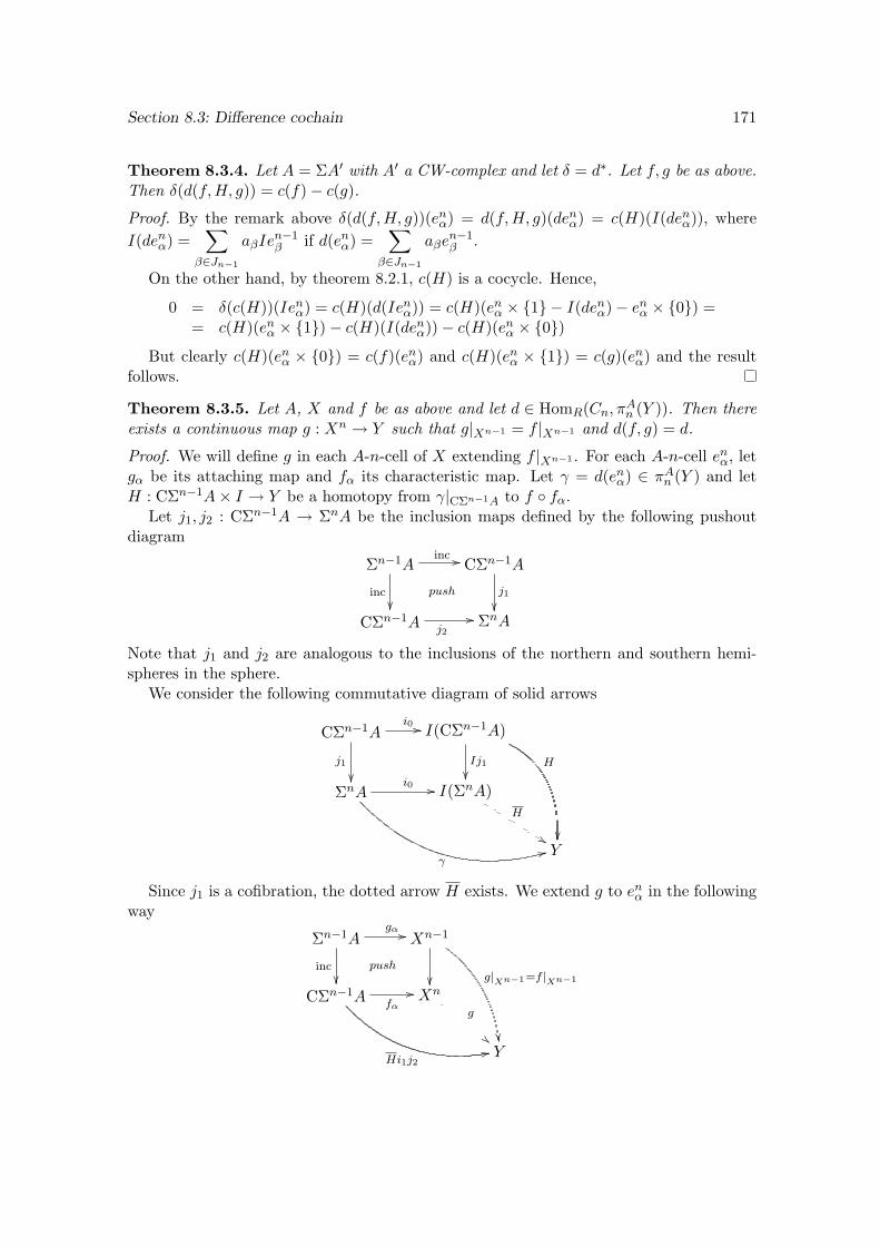
Section 8.3: Difference cochain 171
Theorem 8.3.4. Let A = ΣA′ with A′ a CW-complex and let δ = d∗. Let f, g be as above.Then δ(d(f,H, g)) = c(f)− c(g).
Proof. By the remark above δ(d(f,H, g))(enα) = d(f,H, g)(denα) = c(H)(I(denα)), whereI(denα) =
∑β∈Jn−1
aβIen−1β if d(enα) =
∑β∈Jn−1
aβen−1β .
On the other hand, by theorem 8.2.1, c(H) is a cocycle. Hence,
0 = δ(c(H))(Ienα) = c(H)(d(Ienα)) = c(H)(enα × 1 − I(denα)− enα × 0) == c(H)(enα × 1)− c(H)(I(denα))− c(H)(enα × 0)
But clearly c(H)(enα × 0) = c(f)(enα) and c(H)(enα × 1) = c(g)(enα) and the resultfollows.
Theorem 8.3.5. Let A, X and f be as above and let d ∈ HomR(Cn, πAn (Y )). Then thereexists a continuous map g : Xn → Y such that g|Xn−1 = f |Xn−1 and d(f, g) = d.
Proof. We will define g in each A-n-cell of X extending f |Xn−1 . For each A-n-cell enα, letgα be its attaching map and fα its characteristic map. Let γ = d(enα) ∈ πAn (Y ) and letH : CΣn−1A× I → Y be a homotopy from γ|CΣn−1A to f fα.
Let j1, j2 : CΣn−1A → ΣnA be the inclusion maps defined by the following pushoutdiagram
Σn−1Ainc //
inc
push
CΣn−1A
j1
CΣn−1A j2// ΣnA
Note that j1 and j2 are analogous to the inclusions of the northern and southern hemi-spheres in the sphere.
We consider the following commutative diagram of solid arrows
CΣn−1Ai0 //
j1
I(CΣn−1A)
Ij1
H
ΣnAi0 //
γ33
I(ΣnA)H
%%Y
Since j1 is a cofibration, the dotted arrow H exists. We extend g to enα in the followingway
Σn−1Agα //
inc
push
Xn−1
g|Xn−1=f |Xn−1
CΣn−1A fα
//
Hi1j222
Xn
g
""Y
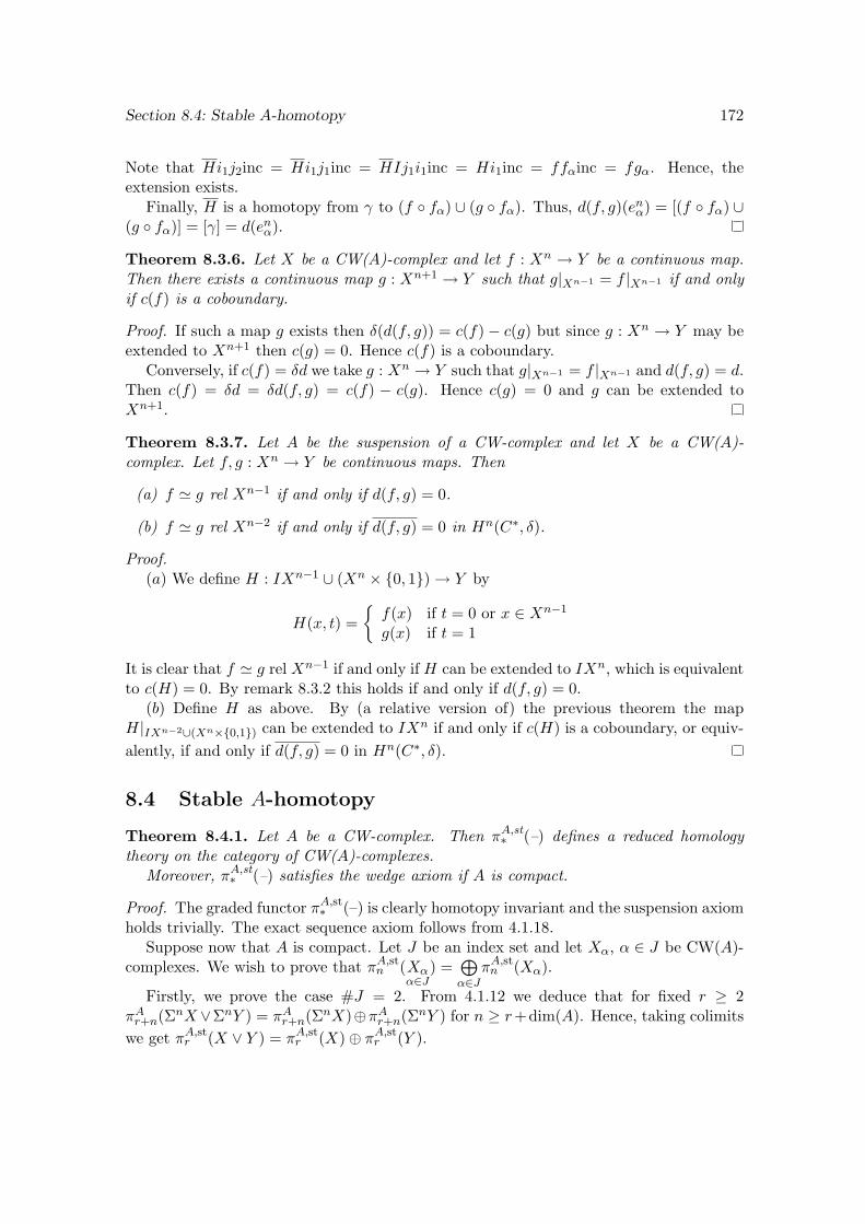
Section 8.4: Stable A-homotopy 172
Note that Hi1j2inc = Hi1j1inc = HIj1i1inc = Hi1inc = ffαinc = fgα. Hence, theextension exists.
Finally, H is a homotopy from γ to (f fα) ∪ (g fα). Thus, d(f, g)(enα) = [(f fα) ∪(g fα)] = [γ] = d(enα).
Theorem 8.3.6. Let X be a CW(A)-complex and let f : Xn → Y be a continuous map.Then there exists a continuous map g : Xn+1 → Y such that g|Xn−1 = f |Xn−1 if and onlyif c(f) is a coboundary.
Proof. If such a map g exists then δ(d(f, g)) = c(f)− c(g) but since g : Xn → Y may beextended to Xn+1 then c(g) = 0. Hence c(f) is a coboundary.
Conversely, if c(f) = δd we take g : Xn → Y such that g|Xn−1 = f |Xn−1 and d(f, g) = d.Then c(f) = δd = δd(f, g) = c(f) − c(g). Hence c(g) = 0 and g can be extended toXn+1.
Theorem 8.3.7. Let A be the suspension of a CW-complex and let X be a CW(A)-complex. Let f, g : Xn → Y be continuous maps. Then
(a) f ' g rel Xn−1 if and only if d(f, g) = 0.
(b) f ' g rel Xn−2 if and only if d(f, g) = 0 in Hn(C∗, δ).
Proof.(a) We define H : IXn−1 ∪ (Xn × 0, 1) → Y by
H(x, t) =f(x) if t = 0 or x ∈ Xn−1
g(x) if t = 1
It is clear that f ' g rel Xn−1 if and only if H can be extended to IXn, which is equivalentto c(H) = 0. By remark 8.3.2 this holds if and only if d(f, g) = 0.
(b) Define H as above. By (a relative version of) the previous theorem the mapH|IXn−2∪(Xn×0,1) can be extended to IXn if and only if c(H) is a coboundary, or equiv-alently, if and only if d(f, g) = 0 in Hn(C∗, δ).
8.4 Stable A-homotopy
Theorem 8.4.1. Let A be a CW-complex. Then πA,st∗ (–) defines a reduced homologytheory on the category of CW(A)-complexes.
Moreover, πA,st∗ (–) satisfies the wedge axiom if A is compact.
Proof. The graded functor πA,st∗ (–) is clearly homotopy invariant and the suspension axiomholds trivially. The exact sequence axiom follows from 4.1.18.
Suppose now that A is compact. Let J be an index set and let Xα, α ∈ J be CW(A)-complexes. We wish to prove that πA,stn (Xα
α∈J) =
⊕α∈J
πA,stn (Xα).
Firstly, we prove the case #J = 2. From 4.1.12 we deduce that for fixed r ≥ 2πAr+n(Σ
nX ∨ΣnY ) = πAr+n(ΣnX)⊕πAr+n(ΣnY ) for n ≥ r+dim(A). Hence, taking colimits
we get πA,str (X ∨ Y ) = πA,str (X)⊕ πA,str (Y ).
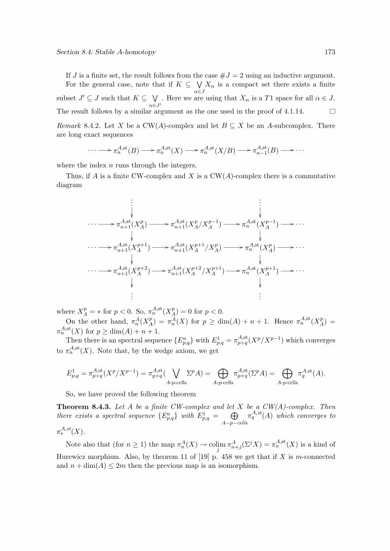
Section 8.4: Stable A-homotopy 173
If J is a finite set, the result follows from the case #J = 2 using an inductive argument.For the general case, note that if K ⊆
∨α∈J
Xα is a compact set there exists a finite
subset J ′ ⊆ J such that K ⊆∨α∈J ′
. Here we are using that Xα is a T1 space for all α ∈ J .
The result follows by a similar argument as the one used in the proof of 4.1.14.
Remark 8.4.2. Let X be a CW(A)-complex and let B ⊆ X be an A-subcomplex. Thereare long exact sequences
. . . // πA,stn (B) // πA,stn (X) // πA,stn (X/B) // πA,stn−1(B) // . . .
where the index n runs through the integers.Thus, if A is a finite CW-complex and X is a CW(A)-complex there is a commutative
diagram
...
...
. . . // πA,stn+1(X
pA) //
πA,stn+1(XpA/X
p−1A ) // πA,stn (Xp−1
A ) //
. . .
. . . // πA,stn+1(Xp+1A ) //
πA,stn+1(Xp+1A /Xp
A) // πA,stn (XpA) //
. . .
. . . // πA,stn+1(Xp+2A ) //
πA,stn+1(Xp+2A /Xp+1
A ) // πA,stn (Xp+1A ) //
. . .
......
where XpA = ∗ for p < 0. So, πA,stn (Xp
A) = 0 for p < 0.On the other hand, πAn (Xp
A) = πAn (X) for p ≥ dim(A) + n + 1. Hence πA,stn (XpA) =
πA,stn (X) for p ≥ dim(A) + n+ 1.Then there is an spectral sequence Eap,q with E1
p,q = πA,stp+q (Xp/Xp−1) which converges
to πA,stn (X). Note that, by the wedge axiom, we get
E1p,q = πA,stp+q (X
p/Xp−1) = πA,stp+q (∨
A-p-cells
ΣpA) =⊕
A-p-cells
πA,stp+q (ΣpA) =
⊕A-p-cells
πA,stq (A).
So, we have proved the following theorem
Theorem 8.4.3. Let A be a finite CW-complex and let X be a CW(A)-complex. Thenthere exists a spectral sequence Eap,q with E1
p,q =⊕
A−p−cells
πA,stq (A) which converges to
πA,st∗ (X).
Note also that (for n ≥ 1) the map πAn (X) → colimj
πAn+j(ΣjX) = πA,stn (X) is a kind of
Hurewicz morphism. Also, by theorem 11 of [19] p. 458 we get that if X is m-connectedand n+ dim(A) ≤ 2m then the previous map is an isomorphism.
Appendix A
Universal coefficient theorems andKunneth formula
In this appendix we recall some useful formulas for computation of homology and coho-mology groups: the universal coefficient theorems and the Kunneth formula. The firstones relate homology and cohomology groups with coefficients with homology groups withintegral coefficients. The latter helps to compute the homology groups of the product ofspaces from the homology groups of each one.
We begin by recalling some basic facts about Tor and Ext functors.
Proposition A.1. Let G, H and Gi, i ∈ I, be abelian groups.
(a) Tor(G,H) ' Tor(H,G).
(b) Tor(⊕i∈I
Gi,H) '⊕i∈I
Tor(Gi,H).
(c) Tor(G,H) = 0 if G or H is torsionfree.
(d) If T (G) is the torsion subgroup of G then Tor(G,H) ' Tor(T (G),H).
(e) If n ∈ N and µn : G→ G is defined by µn(g) = ng, then Tor(Zn, G) ' ker(µg).
(f) If 0 → A→ B → C → 0 is a short exact sequence, then there is an exact sequence
0 // Tor(G,A) // Tor(G,B) // Tor(G,C) // G⊗A // G⊗B // G⊗ C // 0
Proposition A.2. Let G, H and H ′ be abelian groups. Then
(a) Ext(H ⊕H ′, G) ' Ext(H,G)⊕ Ext(H ′, G).
(b) Ext(H,G) = 0 if H is free.
(c) Ext(Zn, G) ' G/nG.
174
175
Theorem A.3 (Universal coefficient theorem for homology). Let (C∗, d∗) be a chain com-plex of free abelian groups and let G be an abelian group. Then for each n ∈ N there arenatural short exact sequences
0 // Hn(C)⊗G // Hn(C;G) // Tor(Hn−1(C), G) // 0
Moreover, these exact sequences split (but not naturally).
Corollary A.4. Let X be a topological space and let A ⊆ X be a subspace. Then
(a) There exist natural short exact sequences
0 // Hn(X; Z)⊗G // Hn(X;G) // Tor(Hn−1(X; Z), G) // 0
for all n ∈ N, and these exact sequences split, but not naturally.
(b) There exist natural short exact sequences
0 // Hn(X,A; Z)⊗G // Hn(X,A;G) // Tor(Hn−1(X,A; Z), G) // 0
for all n ∈ N, and these exact sequences split, but not naturally.
Corollary A.5. Let X be a topological space and let n ∈ N.
(a) Hn(X; Q) ' Hn(X; Z)⊗Q.
(b) If Hn(X; Z) and Hn−1(X; Z) are finitely generated and p is a prime number thenHn(X; Zp) consists of
• a Zp summand for each Z summand of Hn(X; Z).
• a Zp summand for each Zpk summand of Hn(X; Z) with k ≥ 1.
• a Zp summand for each Zpk summand of Hn−1(X; Z) with k ≥ 1.
Corollary A.6. (a) Let X be a topological space. Then Hn(X; Z) = 0 for all n ≥ 0 ifand only if Hn(X; Q) = 0 for all n ≥ 0 and Hn(X; Zp) = 0 for all n ≥ 0 and for allprime numbers p.
(b) A continuous map f : X → Y induces isomorphisms on integral homology groups ifand only if it induces isomorphisms on homology groups with Q and Zp coefficientsfor all prime numbers p.
Theorem A.7 (Universal coefficient theorem for cohomology). Let (C∗, d∗) be a chaincomplex of free abelian groups and let G be an abelian group. Then for each n ∈ N thereare split exact sequences
0 // Ext(Hn−1(C), G) // Hn(C;G) // Hom(Hn(C), G) // 0
Corollary A.8. Let X be a topological space and let G be an abelian group. Then foreach n ∈ N there are split exact sequences
0 // Ext(Hn−1(X; Z), G) // Hn(X;G) // Hom(Hn(X; Z), G) // 0
176
Corollary A.9. Let (C∗, d∗) be a chain complex of free abelian groups and let G be anabelian group. For n ∈ N let Tn be the torsion subgroup of Hn(C) and let k ∈ N. If Hk(C)and Hk−1(C) are finitely generated then Hn(C; Z) ' (Hn(C)/Tn)⊕ Tn−1.
Corollary A.10. Let G be an abelian group and let f : X → Y be a continuous map suchthat f induces isomorphisms in homology groups. Then f∗ : Hn(X;G) → Hn(Y ;G) is anisomorphism for all n ≥ 0.
We give now the topological Kunneth formula which derives directly from its algebraicversion. However, we will not develop this one here.
Theorem A.11 (Topological Kunneth formula). Let X and Y be CW-complexes and letR be a principal ideal domain. Then, there are natural short exact sequences
0 //⊕
0≤i≤n
(Hi(X)⊗RHn−i(Y )) // Hn(X × Y ) //
⊕0≤i≤n−1
TorR(Hi(X),Hn−1−i(Y )) // 0
for all n ∈ N, where homology means homology with coefficients in R. Moreover, theseshort exact sequences split (but not naturally).
There exists also a relative version of this formula which can be found in [8]. From thisrelative version we can deduce the reduced Kunneth formula:
Theorem A.12 (Reduced Kunneth formula). Let X and Y be CW-complexes with basepoints x0 and y0 respectively and let R be a principal ideal domain. Then, there are naturalshort exact sequences
0 //⊕
0≤i≤n
(Hi(X)⊗RHn−i(Y )) // Hn(X ∧ Y ) //
⊕0≤i≤n−1
TorR(Hi(X), Hn−1−i(Y )) // 0
for all n ∈ N, where (reduced) homology means (reduced) homology with coefficients inR and where X ∧ Y denotes the smash product of X and Y , i.e. X ∧ Y = X × Y/(X ×y0 ∪ x0 × Y ). Moreover, these short exact sequences split (but not naturally).
In particular, if Y = Sr, we obtain isomorphisms Hn(X) ' Hn+r(ΣrX).Also, if Y is a Moore space we obtain the following corollary.
Corollary A.13. Let G be an abelian group, let r ∈ N and let Y be a Moore space oftype (G, r). Let X be a CW-complex and let n ∈ N. Then there are natural isomorphismsHn(X;G) ' Hn+r(X ∧ Y ; Z).
Bibliography
[1] Aguilar, M.; Gitler, S. and Prieto, C. Algebraic topology from a homotopical viewpoint.Springer. 2002.
[2] Baues, H.-J. Algebraic Homotopy. Cambridge studies in advanced mathematics. 15.Cambridge University Press. 1989.
[3] Brown, R. Topology and Groupoids: A geometric account of general Topology, homo-topy types and the fundamental grupoid. Booksurge. 2006.
[4] Chacholski, W. A generalization of the triad theorem of Blakers-Massey. Topology36 (1997), no. 6, 1381–1400.
[5] Dror Farjoun, E. Cellular spaces, null spaces and homotopy localization. Lecture Notesin Mathematics, 1622.
[6] Federer, H. A study of function spaces by spectral sequences. Trans. Amer. Math. Soc.82 (1956), 340–361.
[7] Fritsch, R. and Piccinini, R. A. Cellular structures in topology. Cambridge studies inadvanced mathematics. 19. Cambridge University Press. 1990.
[8] Hatcher, A. Algebraic Topology. Cambridge University Press. 2002.
[9] Hatcher, A. Spectral Sequences in Algebraic Topology.Available in http://www.math.cornell.edu/ hatcher/SSAT/SSATpage.html
[10] Mc Cleary, J. A user’s guide to spectral sequences. Cambridge University Press. 2001.
[11] May, J.P. A concise course in algebraic topology. The University of Chicago Press.1999.
[12] Minian, E.G. Complexes in Cat. Topology and its Applications 119 (2002) 41–51.
[13] Minian, E.G. and Ottina, E.M. A geometric decomposition of spaces into cells ofdifferent types. Journal of Homotopy and Related Structures 1 (2006) 245–271.
[14] Minian, E.G. and Ottina, E.M. A geometric decomposition of spaces into cells ofdifferent types II: Homology theory. Topology and its Applications 155 (2008) 1777–1785.
177
178
[15] Minian, E.G. and Ottina, E.M. A-homology, A-homotopy, CW(A)-complexes andspectral sequences. Preprint.
[16] Mosher, R. and Tangora, M. Cohomology operations and applications in homotopytheory. Harper & Row, Publishers. 1968.
[17] Serre, J.-P. Homologie singuliere des espaces fibres. Applications. Annals of mathe-matics 54 (1951), 425–505.
[18] Serre, J.-P. Groupes d’homotopie et classes de groupes abeliens. Annals of mathematics58, no. 2 (1953), 258–294.
[19] Spanier, E. H. Algebraic Topology. Springer. 1966.
[20] Switzer, R. Algebraic Topology - Homotopy and homology. Springer. 1975.
[21] Whitehead, G. W. Elements of homotopy theory. Springer. 1978.
[22] Whitehead, J. H. C. Combinatorial homotopy I. Bull. Amer. Math. Soc. 55 (1949),213–245.
[23] Whitehead, J. H. C. Combinatorial homotopy II. Bull. Amer. Math. Soc. 55 (1949),453–496.