Università degli Studi della Basilicata

SCUOLA DI INGEGNERIA

CORSO DI LAUREA IN INGEGNERIA

MECCANICA

Tesi di Laurea in

Macchine e Sistemi Energetici

DESIGN OF A CENTRIFUGAL PUMP FOR AN

EXPANDER CYCLE ROCKET ENGINE

Relatore:

Prof. Ing. Aldo BONFIGLIOLI

Correlatore:

Ing. Angelo LETO

Laureando:

Antonio CANTIANI

Matricola: 41036

ANNO ACCADEMICO 2014/2015

List of contents Chapter 1

1.1 Definitions and fundamentals (2) .................................................................................... 1

1.1.2 Thrust ............................................................................................................................ 2

1.2 Liquid-fuel rocket engines cycles ........................................................................................ 3

1.3 Expander cycle engines ........................................................................................................ 5

1.3.1 Closed expander cycle ................................................................................................... 6

1.3.2 Closed split expander cycle (5) (6) ................................................................................ 8

1.3.3 Closed dual expander cycle ........................................................................................... 8

1.3.4 Open expander cycle ..................................................................................................... 9

1.4 Existing expander cycle systems ........................................................................................ 10

1.4.1 The RL10 engine .................................................................................................... 10

1.4.2 The LE-5 engine .................................................................................................... 12

1.4.3 Vinci ............................................................................................................................ 13

1.5 Liquid propellants .............................................................................................................. 15

1.4.3 Liquid oxygen ........................................................................................................ 18

1.4.4 Liquid hydrogen ..................................................................................................... 19

1.4.5 Methane .................................................................................................................. 19

Chapter 2

2.1 Introduction ........................................................................................................................ 21

2.2 Pump description ................................................................................................................ 23

2.3 Cavitation ........................................................................................................................... 25

2.4 Pump parameters ................................................................................................................ 27

2.5 Pump design methods......................................................................................................... 40

2.5.1 Method 1 ..................................................................................................................... 40

2.5.2 Method 2 ..................................................................................................................... 41

2.5.3 Method 3 ..................................................................................................................... 42

2.6 Volute design ...................................................................................................................... 43

2.6.1 Effect of the volute design on efficiency .................................................................... 44

2.6.2 Volute geometry esteem .............................................................................................. 46

Chapter 3

3.1 Introduction ........................................................................................................................ 48

3.2 Impulse turbines ................................................................................................................. 49

3.3 Velocity-compounded impulse turbine .............................................................................. 49

3.4 Reaction turbine ................................................................................................................. 50

3.5 Impulse turbines design ...................................................................................................... 50

Chapter 4

4.1 Introduction ........................................................................................................................ 55

4.2 CoolProp libraries .............................................................................................................. 55

4.3 MatLab functions: pump.m ................................................................................................ 59

4.4 MatLab functions: bladesNumber.m .................................................................................. 66

4.5 Software test-case ............................................................................................................... 68

Chapter 5

5.1 Turbopump specifics and applications ............................................................................... 73

5.2 Conclusions ........................................................................................................................ 76

Appendix

Appendix A – MatLab additional functions ............................................................................. 77

Appendix B – RL10-3-3A LH2 pump output parameters........................................................ 81

Appendix C– RL10-3-3A LO2 pump output parameters......................................................... 84

Appendix D: Designed methane pump output parameters ....................................................... 86

Introduction

The present work is aimed at designing a centrifugal pump for an expander cycle engine fed

system. In particular, the pump has been designed to work with liquid methane. The choice of

this type of cryogenic working fluid has been driven by the characteristic required by a rocket

propulsion system: the methane has a lower cost and a higher density with respect to the more

commonly used hydrogen. The lower cost is obviously a very appreciated feature; in addition

to this, the higher density allows the design of more compact stages, which reduces the total

weigh and the aerodynamic drag.

The design phase led to the development of a software in MatLab environment. This software

aims to be a tool capable of providing a preliminary design of a generic centrifugal pump, given

certain input data. The CoolProp libraries have played a key role in the software development.

These libraries are an open source tool that, once implemented in MatLab, enabled to easily

determine the thermodynamic variables required for the software calculations.

The developed software passed through a validation process, in which we have performed

various design simulation based on the known data of the hydrogen and oxygen pump of a

RL10A-3-3A; the results have shown an acceptable error margin.

Later, we moved to the design of the methane pump. It has been design with input data that

should provide comparable performances to those of the methane pump developed by the Italian

company AVIO for the LM10-Mira engine, which is currently under development in

collaboration with the Russian KBKhA.

In addition to the various graph of the velocity triangles and 2-Dimensional models of the

impeller, a 3-Dimensional model of the pump has been developed through the use of

SolidWorks

1

Chapter 1

Liquid-fuel rocket engines

Since the beginning of the “rocket era” liquid-fuel engines have been the most widely used

rocket engines. They passed through a long improvement process, which has led to engines that

develop higher thrust, weigh less and are more reliable. The main goal of interest is to increase

the payload, cost reduction, reliability improvement and design reusable launch vehicles (1).

1.1 Definitions and fundamentals (2)

The function of rockets engines is to convert the chemical energy provided by the propellant

into thrust, through the combustion process.

The total impulse It is defined as the thrust force F (which may be time dependent) integrated

over the burning time t, as shown by equation (1.1).

𝐼𝑡 = ∫ 𝐹(𝑡)𝑡

0

𝑑𝑡 (1.1)

The total impulse is proportional to the energy released by the propellant.

For constant thrust force and negligible start and stop transients, equation (1.1) reduces to:

𝐼𝑡 = 𝐹 𝑡 (1.2)

The specific impulse Isp is the total impulse per unit of weight flow rate of propellant. It is an

important parameter that describes the performances of the rocket propulsion system. If we

denote by 𝑔0 the acceleration of gravity at sea-level and by �� the mass flow rate of propellant,

then equation (1.3) returns the specific impulse.

𝐼𝑠𝑝 =∫ 𝐹

𝑡

0𝑑𝑡

𝑔0 ∫ �� 𝑑𝑡𝑡

0

(1.3)

This expression gives a time-averaged specific impulse value. For constant thrust and propellant

flow, the equation (1.3) can be simplified as follows:

𝐼𝑠𝑝 =𝐼𝑡

𝑚𝑝 𝑔0 (1.4)

where 𝑚𝑝 is the total effective propellant mass.

Chapter 1 __________________________________________________________________

2

In the SI system Isp is expressed in seconds, however it does not represent a measure of elapsed

time.

The exhaust velocity in the rocket nozzle is not uniform over the entire cross-section. Since the

velocity profile is difficult to measure accurately, a uniform axial velocity c is assumed, which

allows a one-dimensional description of the problem. This effective exhaust velocity c is the

equivalent velocity at which the propellants should be ejected from the vehicle to achieve the

engine specific impulse. It is defined as

𝑐 = 𝐼𝑠𝑝𝑔0 =𝐹

�� (1.5)

It the SI system, the effective exhaust velocity is expressed in meters per seconds. Since the

effective exhaust velocity c and the specific impulse 𝐼𝑠𝑝 only differ by an arbitrary constant 𝑔0,

either one or the other can be used to measure the rocket performances.

The mass ratio MR of a vehicle or a particular vehicle stage is defined as the final mass mf

(after the rocket has consumed all usable propellant) divided by the initial mass m0:

𝑀𝑅 =𝑚𝑓

𝑚0 (1.6)

1.1.2 Thrust

The thrust is the force produced by a rocket propulsion system acting upon a vehicle. In a

simplified way, it is the reaction experienced by its structure due to the ejection of mass at high

velocity. This phenomenon is a consequence of the law of conservation of linear momentum:

the high-pressure gases generated by the combustion of the propellant are accelerated by the

nozzle and ejected at high velocity. The momentum of the combustion products is balanced by

a momentum imparted to the vehicle in the opposite direction. In rocket propulsion relatively

small masses are involved, which are carried with the vehicle and ejected at high velocities.

The thrust due to the change in momentum is given by:

𝐹 =𝑑𝑚

𝑑𝑡𝑣2 = ��𝑣2 (1.7)

This force represents the total propulsion force when the nozzle exit pressure equals the external

pressure. To be more precise, also the pressure of the surrounding fluid has an influence upon

the thrust.

____________________________________________ 1.2 Liquid-fuel rocket engines cycles

3

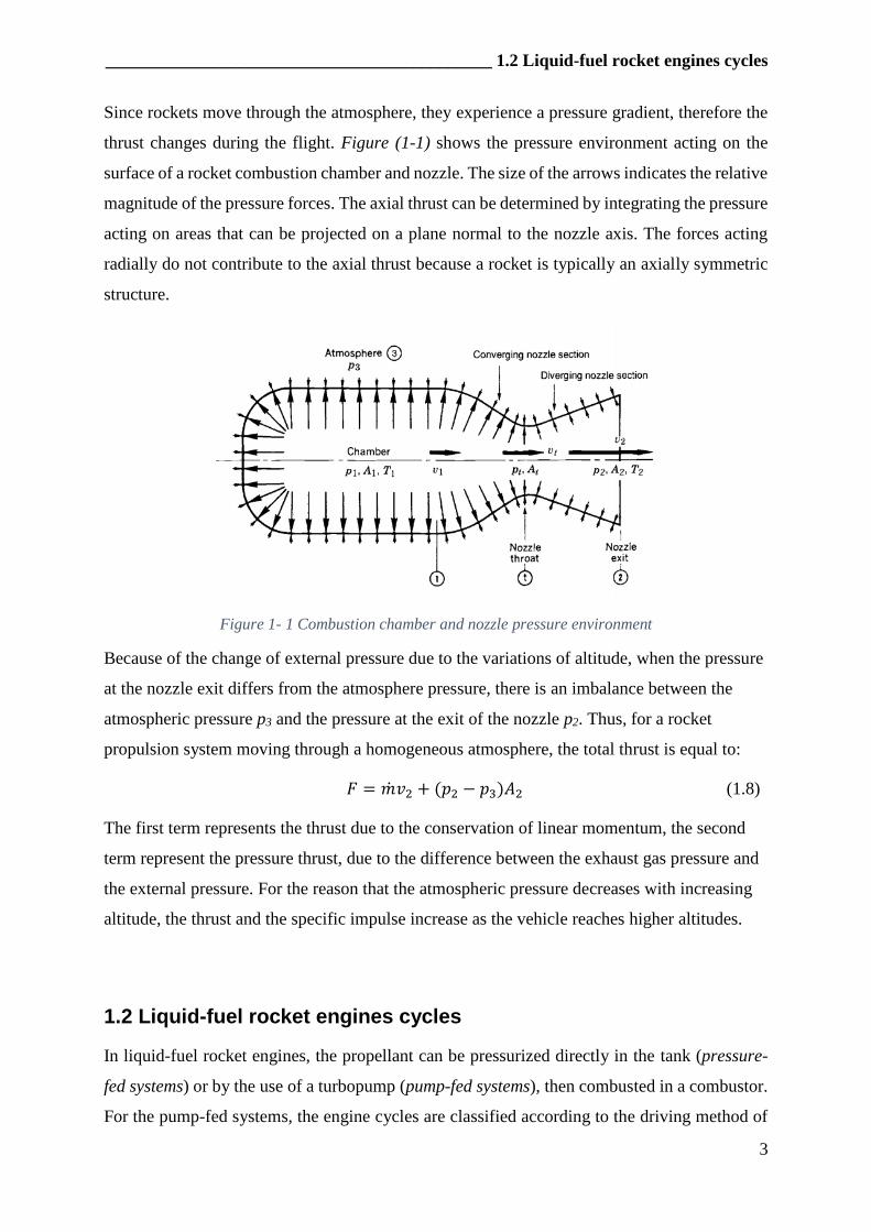
Since rockets move through the atmosphere, they experience a pressure gradient, therefore the

thrust changes during the flight. Figure (1-1) shows the pressure environment acting on the

surface of a rocket combustion chamber and nozzle. The size of the arrows indicates the relative

magnitude of the pressure forces. The axial thrust can be determined by integrating the pressure

acting on areas that can be projected on a plane normal to the nozzle axis. The forces acting

radially do not contribute to the axial thrust because a rocket is typically an axially symmetric

structure.

Figure 1- 1 Combustion chamber and nozzle pressure environment

Because of the change of external pressure due to the variations of altitude, when the pressure

at the nozzle exit differs from the atmosphere pressure, there is an imbalance between the

atmospheric pressure p3 and the pressure at the exit of the nozzle p2. Thus, for a rocket

propulsion system moving through a homogeneous atmosphere, the total thrust is equal to:

𝐹 = ��𝑣2 + (𝑝2 − 𝑝3)𝐴2 (1.8)

The first term represents the thrust due to the conservation of linear momentum, the second

term represent the pressure thrust, due to the difference between the exhaust gas pressure and

the external pressure. For the reason that the atmospheric pressure decreases with increasing

altitude, the thrust and the specific impulse increase as the vehicle reaches higher altitudes.

1.2 Liquid-fuel rocket engines cycles

In liquid-fuel rocket engines, the propellant can be pressurized directly in the tank (pressure-

fed systems) or by the use of a turbopump (pump-fed systems), then combusted in a combustor.

For the pump-fed systems, the engine cycles are classified according to the driving method of

Chapter 1 __________________________________________________________________

4

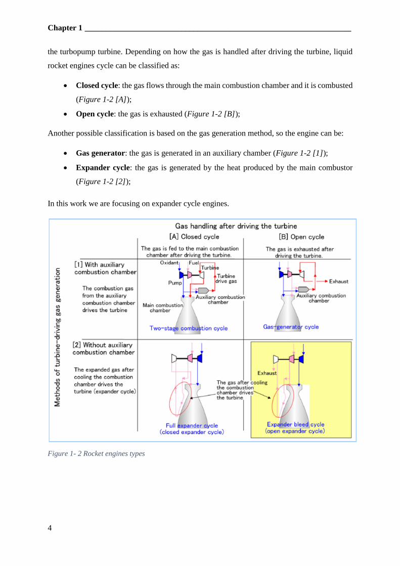
the turbopump turbine. Depending on how the gas is handled after driving the turbine, liquid

rocket engines cycle can be classified as:

Closed cycle: the gas flows through the main combustion chamber and it is combusted

(Figure 1-2 [A]);

Open cycle: the gas is exhausted (Figure 1-2 [B]);

Another possible classification is based on the gas generation method, so the engine can be:

Gas generator: the gas is generated in an auxiliary chamber (Figure 1-2 [1]);

Expander cycle: the gas is generated by the heat produced by the main combustor

(Figure 1-2 [2]);

In this work we are focusing on expander cycle engines.

Figure 1- 2 Rocket engines types

____________________________________________________ 1.3 Expander cycle engines

5

1.3 Expander cycle engines

The working principle of an expander cycle engine is to increase the energy of the propellant

fluid (and also of the oxidizer fluid in some variants of the cycle) thanks to the heat produced

by the combustion chamber. The heat is transferred to the fluid using the cooling jacket placed

around the combustion chamber and the nozzle. This high-energy fluid goes into a turbine that

uses part of the fluid energy to drive the propellant and oxidizer turbopump. Once it has been

discharged from the turbine, it is injected into the combustion chamber and burned in the case

of closed expander cycles, or exhausted if the engine works with an open expander cycle.

Generally, cryogenic propellants are used, such as liquid hydrogen (LH2) and liquid oxygen

(LOX).

The main elements of an expander cycle engine are:

Tank system (fuel tank, oxidizer tank);

Turbopump system;

Cooling system;

Injector system;

Main combustion chamber;

Thrust chamber;

The turbopump has the purpose of increasing the fluid pressure to a value able to satisfy the

pressure drop in the cooling system and pipes, the fuel expansion in the turbine and the required

pressure at the injectors.

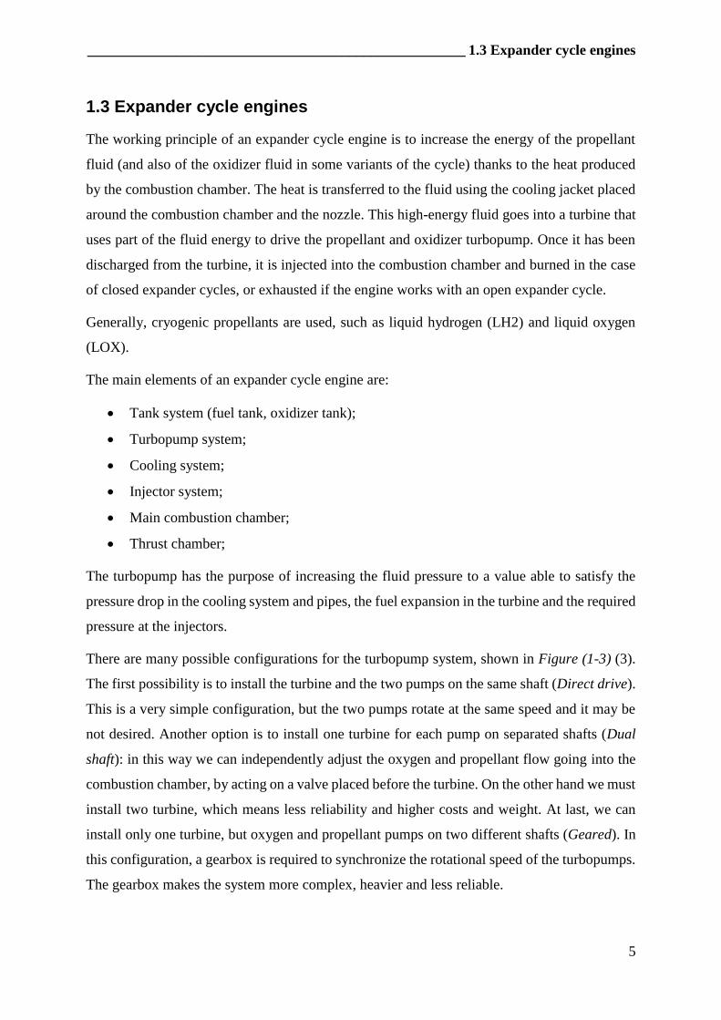
There are many possible configurations for the turbopump system, shown in Figure (1-3) (3).

The first possibility is to install the turbine and the two pumps on the same shaft (Direct drive).

This is a very simple configuration, but the two pumps rotate at the same speed and it may be

not desired. Another option is to install one turbine for each pump on separated shafts (Dual

shaft): in this way we can independently adjust the oxygen and propellant flow going into the

combustion chamber, by acting on a valve placed before the turbine. On the other hand we must

install two turbine, which means less reliability and higher costs and weight. At last, we can

install only one turbine, but oxygen and propellant pumps on two different shafts (Geared). In

this configuration, a gearbox is required to synchronize the rotational speed of the turbopumps.

The gearbox makes the system more complex, heavier and less reliable.

Chapter 1 __________________________________________________________________

6

Figure 1- 3 Pump-turbine drive systems

The reliability of the expander cycle engines is provided by the simple configuration and the

relatively low structural and thermal load on the turbine side.

The limit of this engine cycle is the inlet turbine temperature, since we have a limited area

where we can place the cooling jacket. The problem lies with the square-cubic rule: as the size

of the nozzle increases with increasing thrust, the nozzle surface area increases as the square of

the diameter, but the volume of propellant that must be heated increases with the cube of the

diameter. Therefore, there exists a maximum engine size beyond which there is no longer

enough nozzle area to heat the propellant enough to drive the turbine and, therefore, the

turbopumps (4).

1.3.1 Closed expander cycle

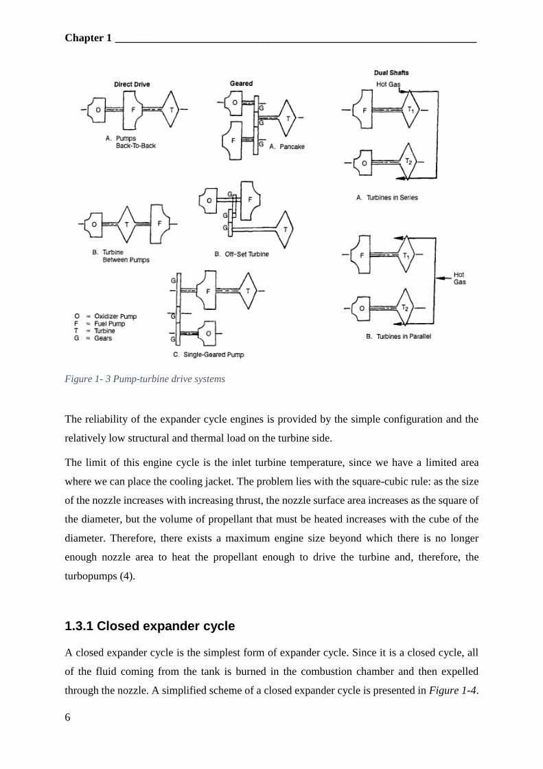
A closed expander cycle is the simplest form of expander cycle. Since it is a closed cycle, all

of the fluid coming from the tank is burned in the combustion chamber and then expelled

through the nozzle. A simplified scheme of a closed expander cycle is presented in Figure 1-4.

____________________________________________________ 1.3 Expander cycle engines

7

Both fuel and the oxidizer fluids go

through a turbopump that increase their

pressure. The oxidizer is then directly

injected into the combustion chamber.

The propellant travels along the

combustion chamber and the nozzle to

increase its temperature. Usually the

combustion chamber is cooled first,

because most of the heat is transferred

in this part of the engine, then the

nozzle is being cooled. This high

energy fluid is now delivered to the

turbine. The turbine must provide

enough power to compress the

propellant and oxidizer to the pressure

level needed. After that, the propellant

goes through some injector and enters

the combustion chamber.

The pressure that the fuel pump has to generate is obtained by adding the pressure generated by

the combustion chamber with the pressure drops that occurs into the cooling system, the

injection system and the turbines pressure drop:

ΔP𝐹𝑃 = 𝑃𝑐 + ΔP𝑖𝑛𝑗 + ΔP𝑡 + ΔP𝑐𝑜𝑜𝑙 (1.9)

Regarding the oxidizer fluid, the pressure that the oxidizer pump has to generate equals to

ΔP𝑂𝑃 = 𝑃𝑐 + ΔP𝑖𝑛𝑗 (1.10)

With the oxidation (combustion) of the propellant in the combustion chamber, there is a release

of energy and the generation of high-velocity combustion products, accelerated by the nozzle

to a supersonic speed in order to provide a high thrust level.

Figure 1- 4: Closed expander cycle schematic. MFV:

Main Fuel Valve, MOV: Main Oxidizer Valve, OTBV:

Oxidizer Turbine Bypass Valve (for regulation)

Chapter 1 __________________________________________________________________

8

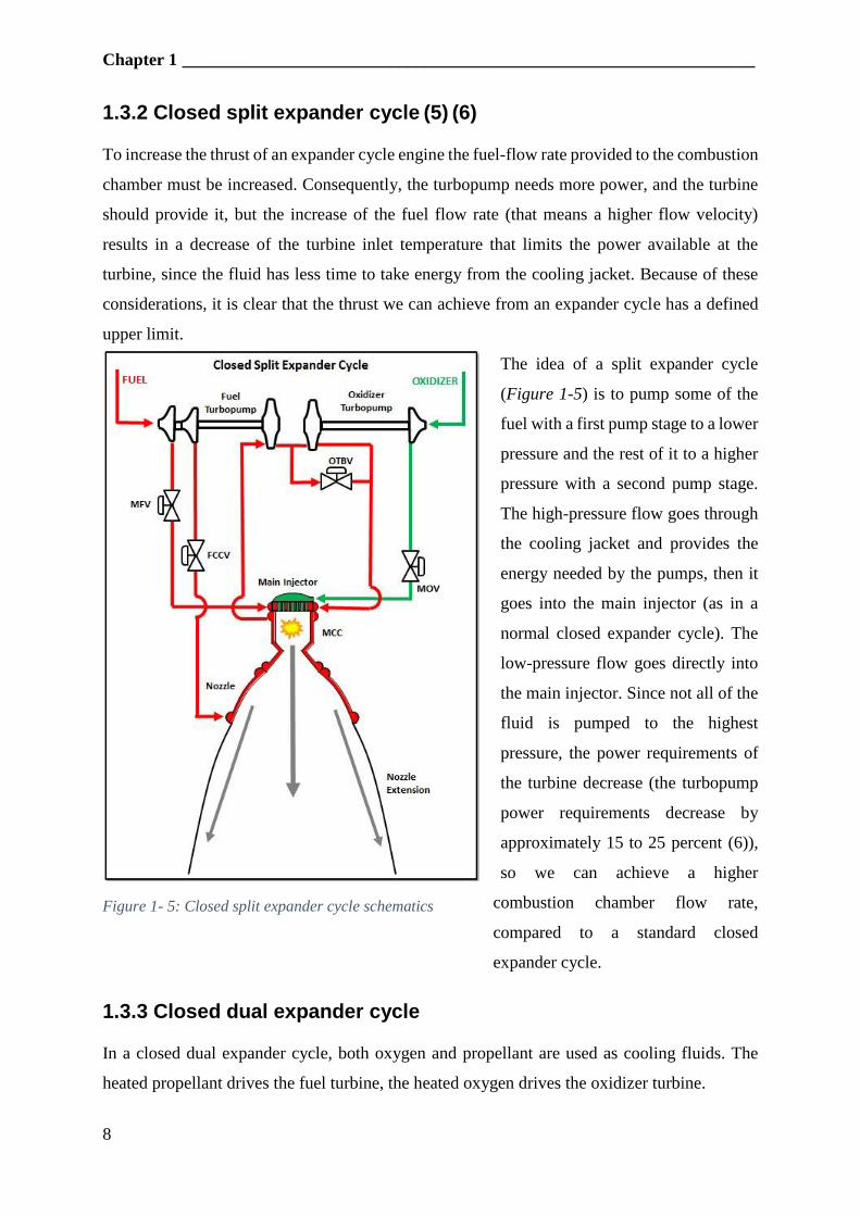
1.3.2 Closed split expander cycle (5) (6)

To increase the thrust of an expander cycle engine the fuel-flow rate provided to the combustion

chamber must be increased. Consequently, the turbopump needs more power, and the turbine

should provide it, but the increase of the fuel flow rate (that means a higher flow velocity)

results in a decrease of the turbine inlet temperature that limits the power available at the

turbine, since the fluid has less time to take energy from the cooling jacket. Because of these

considerations, it is clear that the thrust we can achieve from an expander cycle has a defined

upper limit.

The idea of a split expander cycle

(Figure 1-5) is to pump some of the

fuel with a first pump stage to a lower

pressure and the rest of it to a higher

pressure with a second pump stage.

The high-pressure flow goes through

the cooling jacket and provides the

energy needed by the pumps, then it

goes into the main injector (as in a

normal closed expander cycle). The

low-pressure flow goes directly into

the main injector. Since not all of the

fluid is pumped to the highest

pressure, the power requirements of

the turbine decrease (the turbopump

power requirements decrease by

approximately 15 to 25 percent (6)),

so we can achieve a higher

combustion chamber flow rate,

compared to a standard closed

expander cycle.

1.3.3 Closed dual expander cycle

In a closed dual expander cycle, both oxygen and propellant are used as cooling fluids. The

heated propellant drives the fuel turbine, the heated oxygen drives the oxidizer turbine.

Figure 1- 5: Closed split expander cycle schematics

____________________________________________________ 1.3 Expander cycle engines

9

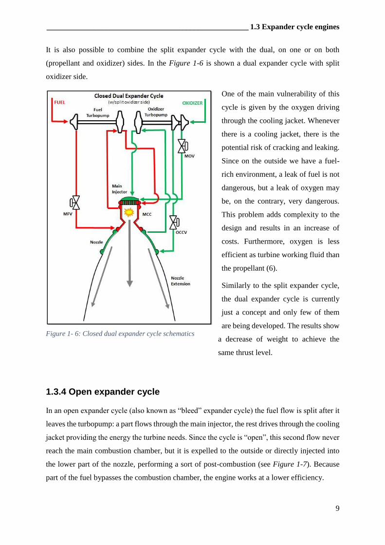
It is also possible to combine the split expander cycle with the dual, on one or on both

(propellant and oxidizer) sides. In the Figure 1-6 is shown a dual expander cycle with split

oxidizer side.

One of the main vulnerability of this

cycle is given by the oxygen driving

through the cooling jacket. Whenever

there is a cooling jacket, there is the

potential risk of cracking and leaking.

Since on the outside we have a fuel-

rich environment, a leak of fuel is not

dangerous, but a leak of oxygen may

be, on the contrary, very dangerous.

This problem adds complexity to the

design and results in an increase of

costs. Furthermore, oxygen is less

efficient as turbine working fluid than

the propellant (6).

Similarly to the split expander cycle,

the dual expander cycle is currently

just a concept and only few of them

are being developed. The results show

a decrease of weight to achieve the

same thrust level.

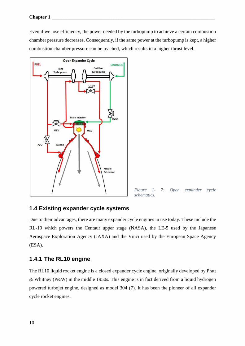
1.3.4 Open expander cycle

In an open expander cycle (also known as “bleed” expander cycle) the fuel flow is split after it

leaves the turbopump: a part flows through the main injector, the rest drives through the cooling

jacket providing the energy the turbine needs. Since the cycle is “open”, this second flow never

reach the main combustion chamber, but it is expelled to the outside or directly injected into

the lower part of the nozzle, performing a sort of post-combustion (see Figure 1-7). Because

part of the fuel bypasses the combustion chamber, the engine works at a lower efficiency.

Figure 1- 6: Closed dual expander cycle schematics

Chapter 1 __________________________________________________________________

10

Even if we lose efficiency, the power needed by the turbopump to achieve a certain combustion

chamber pressure decreases. Consequently, if the same power at the turbopump is kept, a higher

combustion chamber pressure can be reached, which results in a higher thrust level.

Figure 1- 7: Open expander cycle

schematics.

1.4 Existing expander cycle systems

Due to their advantages, there are many expander cycle engines in use today. These include the

RL-10 which powers the Centaur upper stage (NASA), the LE-5 used by the Japanese

Aerospace Exploration Agency (JAXA) and the Vinci used by the European Space Agency

(ESA).

1.4.1 The RL10 engine

The RL10 liquid rocket engine is a closed expander cycle engine, originally developed by Pratt

& Whitney (P&W) in the middle 1950s. This engine is in fact derived from a liquid hydrogen

powered turbojet engine, designed as model 304 (7). It has been the pioneer of all expander

cycle rocket engines.

_____________________________________________ 1.4 Existing expander cycle systems

11

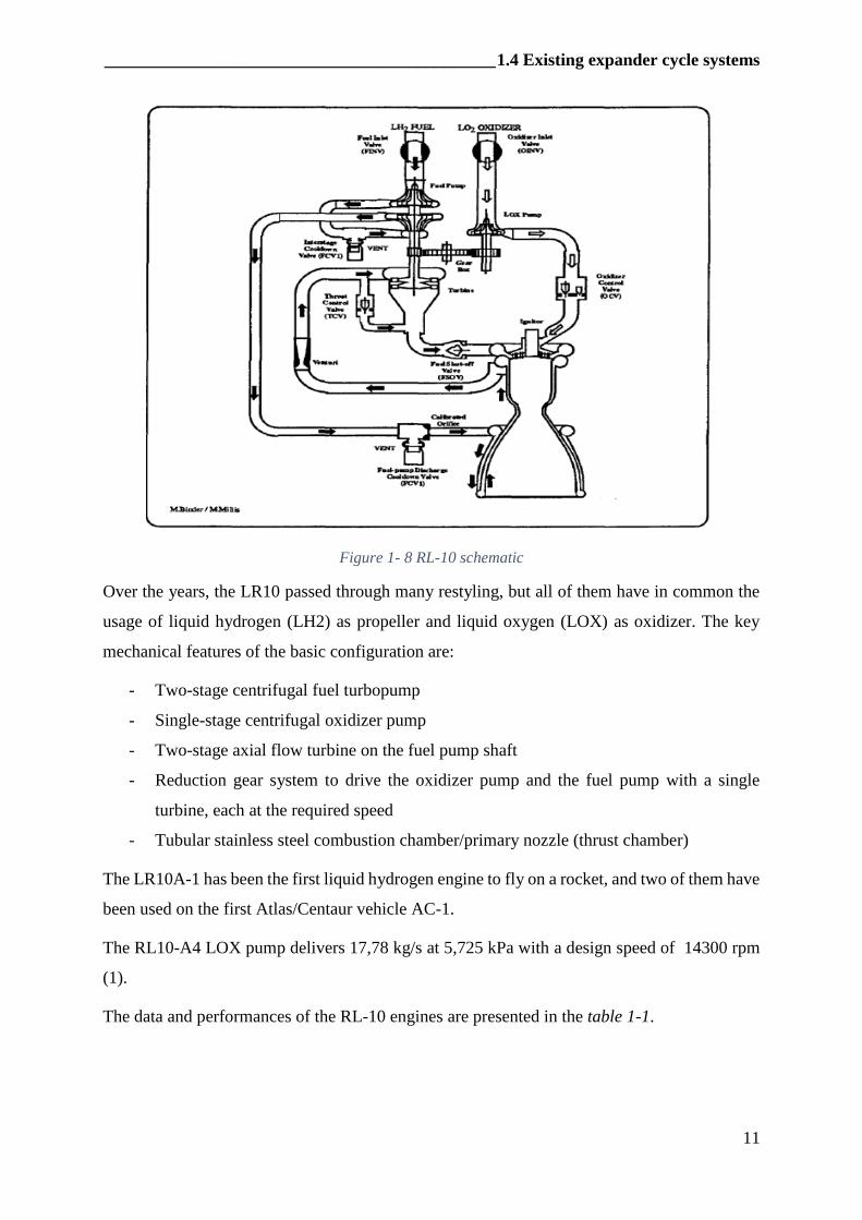
Figure 1- 8 RL-10 schematic

Over the years, the LR10 passed through many restyling, but all of them have in common the

usage of liquid hydrogen (LH2) as propeller and liquid oxygen (LOX) as oxidizer. The key

mechanical features of the basic configuration are:

- Two-stage centrifugal fuel turbopump

- Single-stage centrifugal oxidizer pump

- Two-stage axial flow turbine on the fuel pump shaft

- Reduction gear system to drive the oxidizer pump and the fuel pump with a single

turbine, each at the required speed

- Tubular stainless steel combustion chamber/primary nozzle (thrust chamber)

The LR10A-1 has been the first liquid hydrogen engine to fly on a rocket, and two of them have

been used on the first Atlas/Centaur vehicle AC-1.

The RL10-A4 LOX pump delivers 17,78 kg/s at 5,725 kPa with a design speed of 14300 rpm

(1).

The data and performances of the RL-10 engines are presented in the table 1-1.

Chapter 1 __________________________________________________________________

12

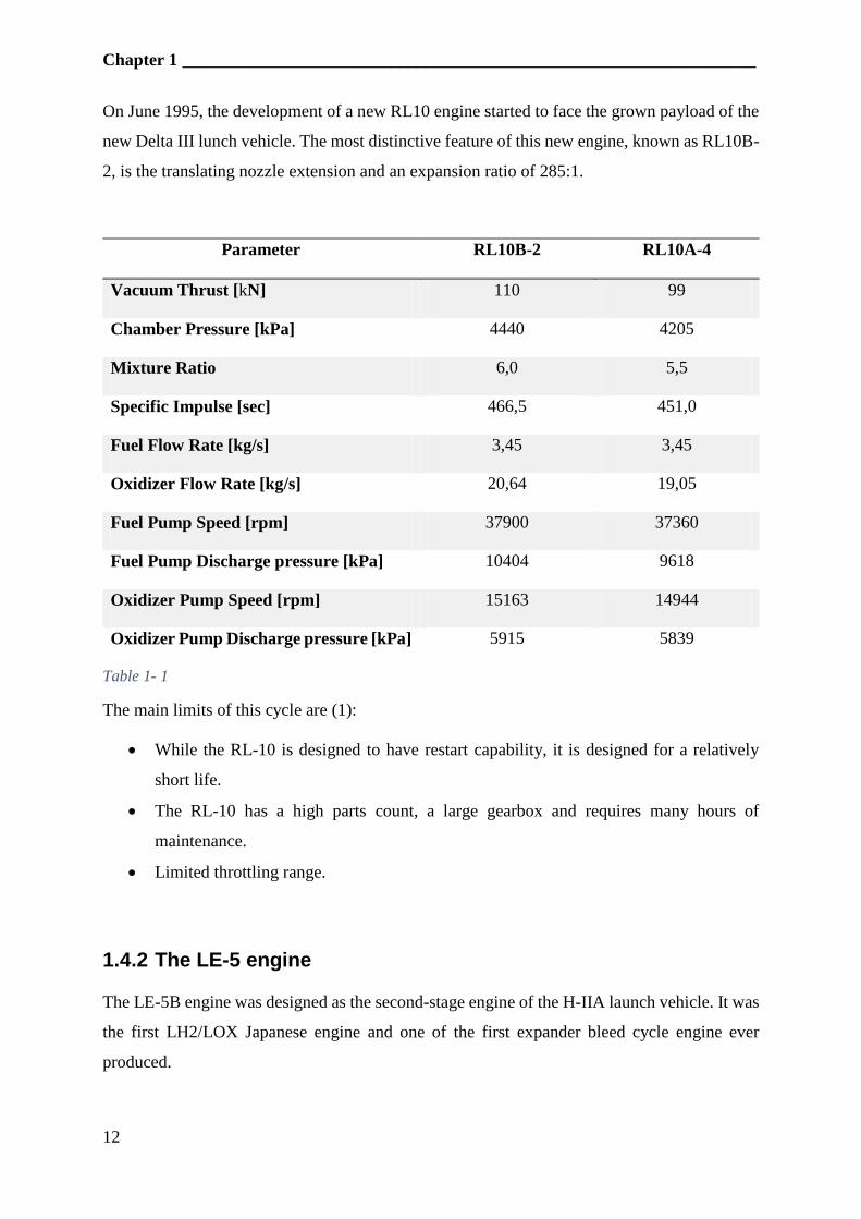
On June 1995, the development of a new RL10 engine started to face the grown payload of the

new Delta III lunch vehicle. The most distinctive feature of this new engine, known as RL10B-

2, is the translating nozzle extension and an expansion ratio of 285:1.

Parameter RL10B-2 RL10A-4

Vacuum Thrust [kN] 110 99

Chamber Pressure [kPa] 4440 4205

Mixture Ratio 6,0 5,5

Specific Impulse [sec] 466,5 451,0

Fuel Flow Rate [kg/s] 3,45 3,45

Oxidizer Flow Rate [kg/s] 20,64 19,05

Fuel Pump Speed [rpm] 37900 37360

Fuel Pump Discharge pressure [kPa] 10404 9618

Oxidizer Pump Speed [rpm] 15163 14944

Oxidizer Pump Discharge pressure [kPa] 5915 5839

Table 1- 1

The main limits of this cycle are (1):

While the RL-10 is designed to have restart capability, it is designed for a relatively

short life.

The RL-10 has a high parts count, a large gearbox and requires many hours of

maintenance.

Limited throttling range.

1.4.2 The LE-5 engine

The LE-5B engine was designed as the second-stage engine of the H-IIA launch vehicle. It was

the first LH2/LOX Japanese engine and one of the first expander bleed cycle engine ever

produced.

_____________________________________________ 1.4 Existing expander cycle systems

13

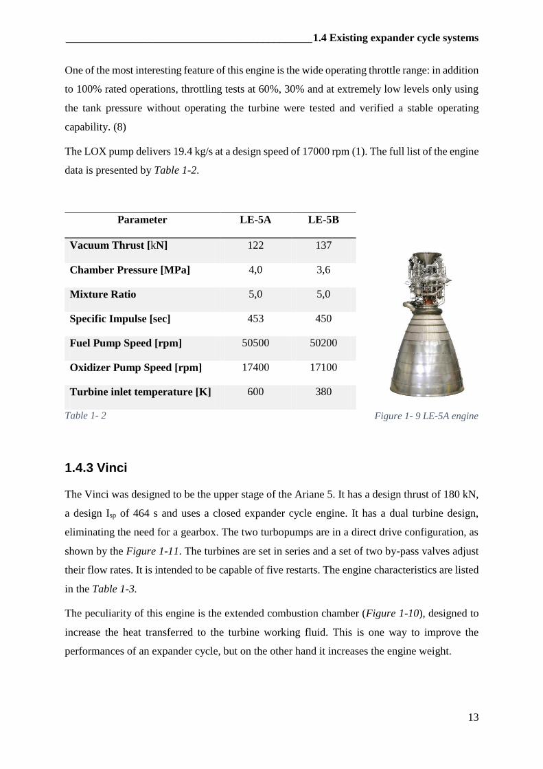
One of the most interesting feature of this engine is the wide operating throttle range: in addition

to 100% rated operations, throttling tests at 60%, 30% and at extremely low levels only using

the tank pressure without operating the turbine were tested and verified a stable operating

capability. (8)

The LOX pump delivers 19.4 kg/s at a design speed of 17000 rpm (1). The full list of the engine

data is presented by Table 1-2.

Parameter LE-5A LE-5B

Vacuum Thrust [kN] 122 137

Chamber Pressure [MPa] 4,0 3,6

Mixture Ratio 5,0 5,0

Specific Impulse [sec] 453 450

Fuel Pump Speed [rpm] 50500 50200

Oxidizer Pump Speed [rpm] 17400 17100

Turbine inlet temperature [K] 600 380

Table 1- 2

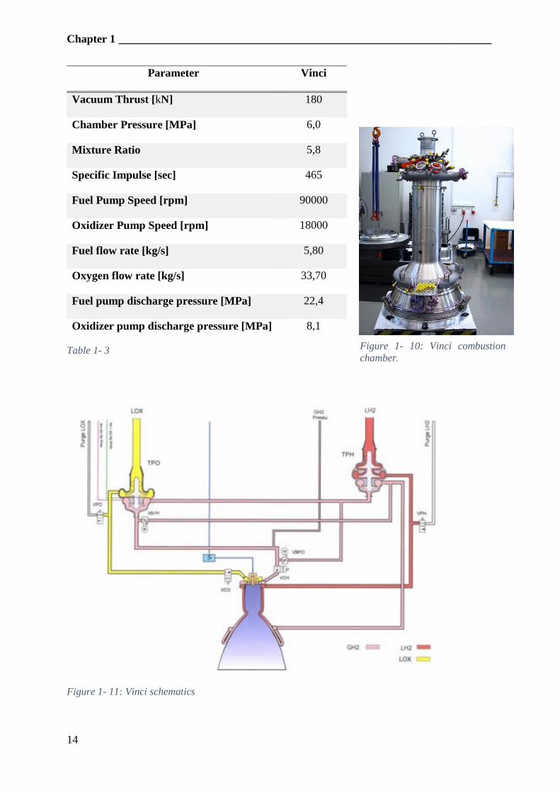
1.4.3 Vinci

The Vinci was designed to be the upper stage of the Ariane 5. It has a design thrust of 180 kN,

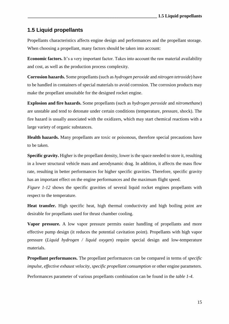
a design Isp of 464 s and uses a closed expander cycle engine. It has a dual turbine design,

eliminating the need for a gearbox. The two turbopumps are in a direct drive configuration, as

shown by the Figure 1-11. The turbines are set in series and a set of two by-pass valves adjust

their flow rates. It is intended to be capable of five restarts. The engine characteristics are listed

in the Table 1-3.

The peculiarity of this engine is the extended combustion chamber (Figure 1-10), designed to

increase the heat transferred to the turbine working fluid. This is one way to improve the

performances of an expander cycle, but on the other hand it increases the engine weight.

Figure 1- 9 LE-5A engine

Chapter 1 __________________________________________________________________

14

Parameter Vinci

Vacuum Thrust [kN] 180

Chamber Pressure [MPa] 6,0

Mixture Ratio 5,8

Specific Impulse [sec] 465

Fuel Pump Speed [rpm] 90000

Oxidizer Pump Speed [rpm] 18000

Fuel flow rate [kg/s] 5,80

Oxygen flow rate [kg/s] 33,70

Fuel pump discharge pressure [MPa] 22,4

Oxidizer pump discharge pressure [MPa] 8,1

Table 1- 3

Figure 1- 11: Vinci schematics

Figure 1- 10: Vinci combustion

chamber.

________________________________________________________ 1.5 Liquid propellants

15

1.5 Liquid propellants

Propellants characteristics affects engine design and performances and the propellant storage.

When choosing a propellant, many factors should be taken into account:

Economic factors. It’s a very important factor. Takes into account the raw material availability

and cost, as well as the production process complexity.

Corrosion hazards. Some propellants (such as hydrogen peroxide and nitrogen tetroxide) have

to be handled in containers of special materials to avoid corrosion. The corrosion products may

make the propellant unsuitable for the designed rocket engine.

Explosion and fire hazards. Some propellants (such as hydrogen peroxide and nitromethane)

are unstable and tend to detonate under certain conditions (temperature, pressure, shock). The

fire hazard is usually associated with the oxidizers, which may start chemical reactions with a

large variety of organic substances.

Health hazards. Many propellants are toxic or poisonous, therefore special precautions have

to be taken.

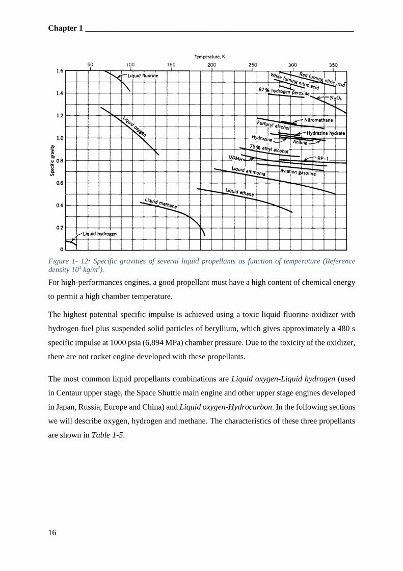
Specific gravity. Higher is the propellant density, lower is the space needed to store it, resulting

in a lower structural vehicle mass and aerodynamic drag. In addition, it affects the mass flow

rate, resulting in better performances for higher specific gravities. Therefore, specific gravity

has an important effect on the engine performances and the maximum flight speed.

Figure 1-12 shows the specific gravities of several liquid rocket engines propellants with

respect to the temperature.

Heat transfer. High specific heat, high thermal conductivity and high boiling point are

desirable for propellants used for thrust chamber cooling.

Vapor pressure. A low vapor pressure permits easier handling of propellants and more

effective pump design (it reduces the potential cavitation point). Propellants with high vapor

pressure (Liquid hydrogen / liquid oxygen) require special design and low-temperature

materials.

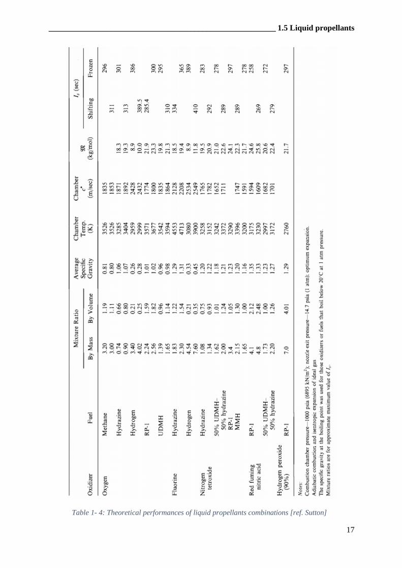
Propellant performances. The propellant performances can be compared in terms of specific

impulse, effective exhaust velocity, specific propellant consumption or other engine parameters.

Performances parameter of various propellants combination can be found in the table 1-4.

Chapter 1 __________________________________________________________________

16

For high-performances engines, a good propellant must have a high content of chemical energy

to permit a high chamber temperature.

The highest potential specific impulse is achieved using a toxic liquid fluorine oxidizer with

hydrogen fuel plus suspended solid particles of beryllium, which gives approximately a 480 s

specific impulse at 1000 psia (6,894 MPa) chamber pressure. Due to the toxicity of the oxidizer,

there are not rocket engine developed with these propellants.

The most common liquid propellants combinations are Liquid oxygen-Liquid hydrogen (used

in Centaur upper stage, the Space Shuttle main engine and other upper stage engines developed

in Japan, Russia, Europe and China) and Liquid oxygen-Hydrocarbon. In the following sections

we will describe oxygen, hydrogen and methane. The characteristics of these three propellants

are shown in Table 1-5.

Figure 1- 12: Specific gravities of several liquid propellants as function of temperature (Reference

density 103 kg/m3).

________________________________________________________ 1.5 Liquid propellants

17

Table 1- 4: Theoretical performances of liquid propellants combinations [ref. Sutton]

Chapter 1 __________________________________________________________________

18

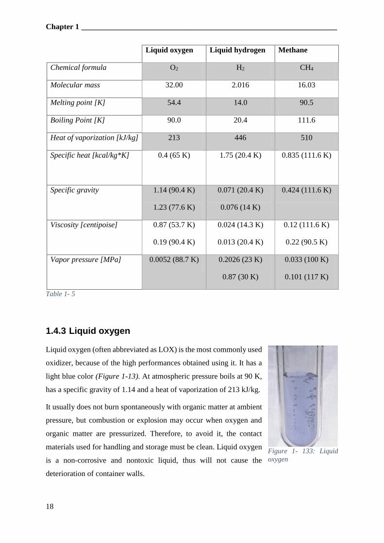
Liquid oxygen Liquid hydrogen Methane

Chemical formula O2 H2 CH4

Molecular mass 32.00 2.016 16.03

Melting point [K] 54.4 14.0 90.5

Boiling Point [K] 90.0 20.4 111.6

Heat of vaporization [kJ/kg] 213 446 510

Specific heat [kcal/kg*K] 0.4 (65 K)

1.75 (20.4 K) 0.835 (111.6 K)

Specific gravity 1.14 (90.4 K)

1.23 (77.6 K)

0.071 (20.4 K)

0.076 (14 K)

0.424 (111.6 K)

Viscosity [centipoise] 0.87 (53.7 K)

0.19 (90.4 K)

0.024 (14.3 K)

0.013 (20.4 K)

0.12 (111.6 K)

0.22 (90.5 K)

Vapor pressure [MPa] 0.0052 (88.7 K) 0.2026 (23 K)

0.87 (30 K)

0.033 (100 K)

0.101 (117 K)

Table 1- 5

1.4.3 Liquid oxygen

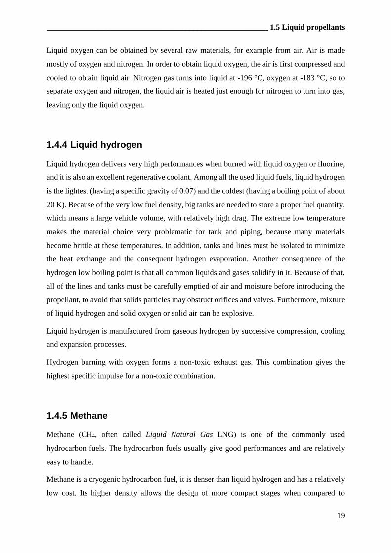
Liquid oxygen (often abbreviated as LOX) is the most commonly used

oxidizer, because of the high performances obtained using it. It has a

light blue color (Figure 1-13). At atmospheric pressure boils at 90 K,

has a specific gravity of 1.14 and a heat of vaporization of 213 kJ/kg.

It usually does not burn spontaneously with organic matter at ambient

pressure, but combustion or explosion may occur when oxygen and

organic matter are pressurized. Therefore, to avoid it, the contact

materials used for handling and storage must be clean. Liquid oxygen

is a non-corrosive and nontoxic liquid, thus will not cause the

deterioration of container walls.

Figure 1- 133: Liquid

oxygen

________________________________________________________ 1.5 Liquid propellants

19

Liquid oxygen can be obtained by several raw materials, for example from air. Air is made

mostly of oxygen and nitrogen. In order to obtain liquid oxygen, the air is first compressed and

cooled to obtain liquid air. Nitrogen gas turns into liquid at -196 °C, oxygen at -183 °C, so to

separate oxygen and nitrogen, the liquid air is heated just enough for nitrogen to turn into gas,

leaving only the liquid oxygen.

1.4.4 Liquid hydrogen

Liquid hydrogen delivers very high performances when burned with liquid oxygen or fluorine,

and it is also an excellent regenerative coolant. Among all the used liquid fuels, liquid hydrogen

is the lightest (having a specific gravity of 0.07) and the coldest (having a boiling point of about

20 K). Because of the very low fuel density, big tanks are needed to store a proper fuel quantity,

which means a large vehicle volume, with relatively high drag. The extreme low temperature

makes the material choice very problematic for tank and piping, because many materials

become brittle at these temperatures. In addition, tanks and lines must be isolated to minimize

the heat exchange and the consequent hydrogen evaporation. Another consequence of the

hydrogen low boiling point is that all common liquids and gases solidify in it. Because of that,

all of the lines and tanks must be carefully emptied of air and moisture before introducing the

propellant, to avoid that solids particles may obstruct orifices and valves. Furthermore, mixture

of liquid hydrogen and solid oxygen or solid air can be explosive.

Liquid hydrogen is manufactured from gaseous hydrogen by successive compression, cooling

and expansion processes.

Hydrogen burning with oxygen forms a non-toxic exhaust gas. This combination gives the

highest specific impulse for a non-toxic combination.

1.4.5 Methane

Methane (CH4, often called Liquid Natural Gas LNG) is one of the commonly used

hydrocarbon fuels. The hydrocarbon fuels usually give good performances and are relatively

easy to handle.

Methane is a cryogenic hydrocarbon fuel, it is denser than liquid hydrogen and has a relatively

low cost. Its higher density allows the design of more compact stages when compared to

Chapter 1 __________________________________________________________________

20

hydrogen, making a lighter vehicle with lower drag, which compensates the lower specific

impulse.

There are some concepts for operating a rocket stage using two fuel, initially with methane and

then switching during flight to hydrogen, but they are not fully developed yet. (2)

21

Chapter 2

Propellant pump

2.1 Introduction

The propellant feed system of a liquid rocket engine is responsible for delivering the propellants

from the tanks to the combustion chamber, at the required flow rate and pressure conditions.

The propellant feed system consists of propellant tanks, feed lines (tubes and ducts), valves and

pressurization devices. Depending on how propellants are pressurized and fed into the

combustion chamber, the feed systems are classified as pressure-fed or pump-fed systems (1).

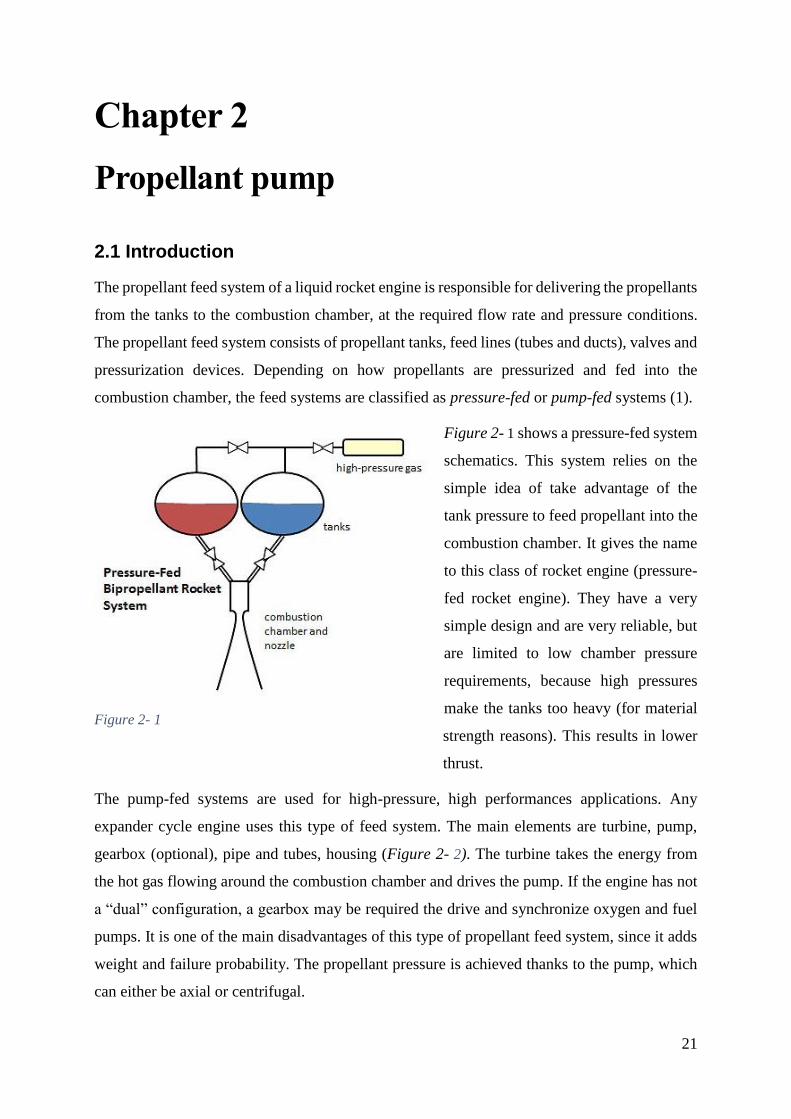
Figure 2- 1 shows a pressure-fed system

schematics. This system relies on the

simple idea of take advantage of the

tank pressure to feed propellant into the

combustion chamber. It gives the name

to this class of rocket engine (pressure-

fed rocket engine). They have a very

simple design and are very reliable, but

are limited to low chamber pressure

requirements, because high pressures

make the tanks too heavy (for material

strength reasons). This results in lower

thrust.

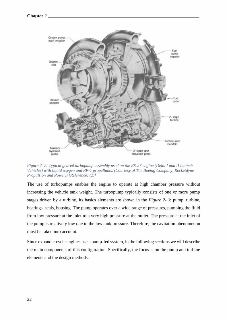
The pump-fed systems are used for high-pressure, high performances applications. Any

expander cycle engine uses this type of feed system. The main elements are turbine, pump,

gearbox (optional), pipe and tubes, housing (Figure 2- 2). The turbine takes the energy from

the hot gas flowing around the combustion chamber and drives the pump. If the engine has not

a “dual” configuration, a gearbox may be required the drive and synchronize oxygen and fuel

pumps. It is one of the main disadvantages of this type of propellant feed system, since it adds

weight and failure probability. The propellant pressure is achieved thanks to the pump, which

can either be axial or centrifugal.

Figure 2- 1

Chapter 2 __________________________________________________________________

22

Figure 2- 2: Typical geared turbopump assembly used on the RS-27 engine (Delta I and II Launch

Vehicles) with liquid oxygen and RP-1 propellants. (Courtesy of The Boeing Company, Rocketdyne

Propulsion and Power.) [Reference: (2)]

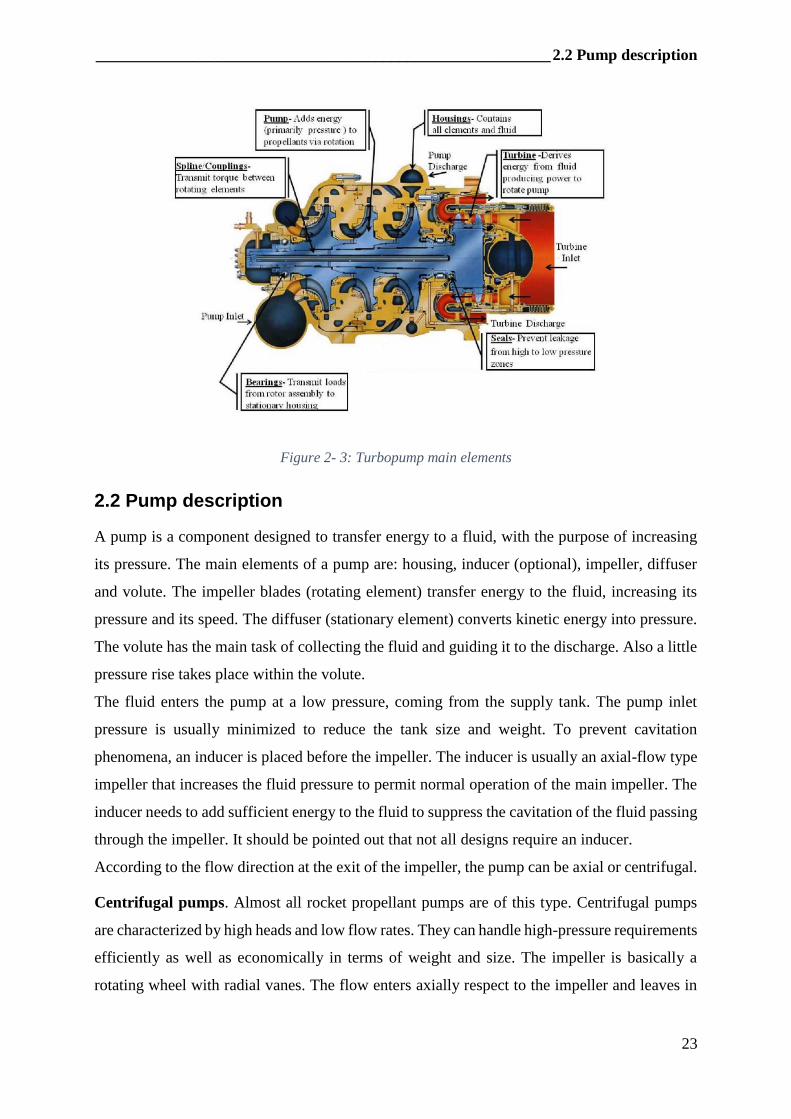
The use of turbopumps enables the engine to operate at high chamber pressure without

increasing the vehicle tank weight. The turbopump typically consists of one or more pump

stages driven by a turbine. Its basics elements are shown in the Figure 2- 3: pump, turbine,

bearings, seals, housing. The pump operates over a wide range of pressures, pumping the fluid

from low pressure at the inlet to a very high pressure at the outlet. The pressure at the inlet of

the pump is relatively low due to the low tank pressure. Therefore, the cavitation phenomenon

must be taken into account.

Since expander cycle engines use a pump-fed system, in the following sections we will describe

the main components of this configuration. Specifically, the focus is on the pump and turbine

elements and the design methods.

_________________________________________________________ 2.2 Pump description

23

Figure 2- 3: Turbopump main elements

2.2 Pump description

A pump is a component designed to transfer energy to a fluid, with the purpose of increasing

its pressure. The main elements of a pump are: housing, inducer (optional), impeller, diffuser

and volute. The impeller blades (rotating element) transfer energy to the fluid, increasing its

pressure and its speed. The diffuser (stationary element) converts kinetic energy into pressure.

The volute has the main task of collecting the fluid and guiding it to the discharge. Also a little

pressure rise takes place within the volute.

The fluid enters the pump at a low pressure, coming from the supply tank. The pump inlet

pressure is usually minimized to reduce the tank size and weight. To prevent cavitation

phenomena, an inducer is placed before the impeller. The inducer is usually an axial-flow type

impeller that increases the fluid pressure to permit normal operation of the main impeller. The

inducer needs to add sufficient energy to the fluid to suppress the cavitation of the fluid passing

through the impeller. It should be pointed out that not all designs require an inducer.

According to the flow direction at the exit of the impeller, the pump can be axial or centrifugal.

Centrifugal pumps. Almost all rocket propellant pumps are of this type. Centrifugal pumps

are characterized by high heads and low flow rates. They can handle high-pressure requirements

efficiently as well as economically in terms of weight and size. The impeller is basically a

rotating wheel with radial vanes. The flow enters axially respect to the impeller and leaves in

Chapter 2 __________________________________________________________________

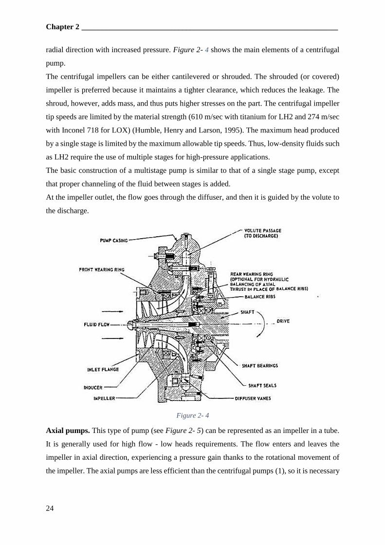
24

radial direction with increased pressure. Figure 2- 4 shows the main elements of a centrifugal

pump.

The centrifugal impellers can be either cantilevered or shrouded. The shrouded (or covered)

impeller is preferred because it maintains a tighter clearance, which reduces the leakage. The

shroud, however, adds mass, and thus puts higher stresses on the part. The centrifugal impeller

tip speeds are limited by the material strength (610 m/sec with titanium for LH2 and 274 m/sec

with Inconel 718 for LOX) (Humble, Henry and Larson, 1995). The maximum head produced

by a single stage is limited by the maximum allowable tip speeds. Thus, low-density fluids such

as LH2 require the use of multiple stages for high-pressure applications.

The basic construction of a multistage pump is similar to that of a single stage pump, except

that proper channeling of the fluid between stages is added.

At the impeller outlet, the flow goes through the diffuser, and then it is guided by the volute to

the discharge.

Figure 2- 4

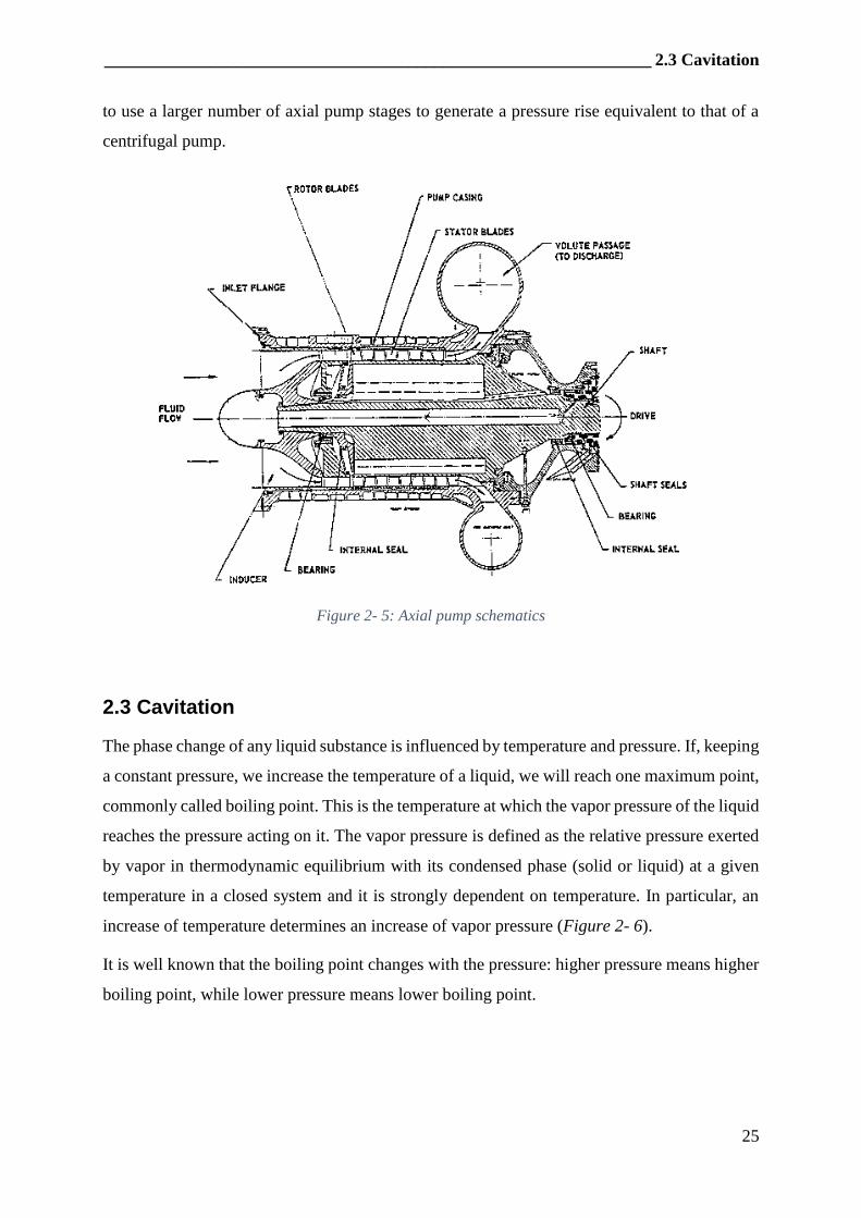
Axial pumps. This type of pump (see Figure 2- 5) can be represented as an impeller in a tube.

It is generally used for high flow - low heads requirements. The flow enters and leaves the

impeller in axial direction, experiencing a pressure gain thanks to the rotational movement of

the impeller. The axial pumps are less efficient than the centrifugal pumps (1), so it is necessary

_______________________________________________________________ 2.3 Cavitation

25

to use a larger number of axial pump stages to generate a pressure rise equivalent to that of a

centrifugal pump.

Figure 2- 5: Axial pump schematics

2.3 Cavitation

The phase change of any liquid substance is influenced by temperature and pressure. If, keeping

a constant pressure, we increase the temperature of a liquid, we will reach one maximum point,

commonly called boiling point. This is the temperature at which the vapor pressure of the liquid

reaches the pressure acting on it. The vapor pressure is defined as the relative pressure exerted

by vapor in thermodynamic equilibrium with its condensed phase (solid or liquid) at a given

temperature in a closed system and it is strongly dependent on temperature. In particular, an

increase of temperature determines an increase of vapor pressure (Figure 2- 6).

It is well known that the boiling point changes with the pressure: higher pressure means higher

boiling point, while lower pressure means lower boiling point.

Chapter 2 __________________________________________________________________

26

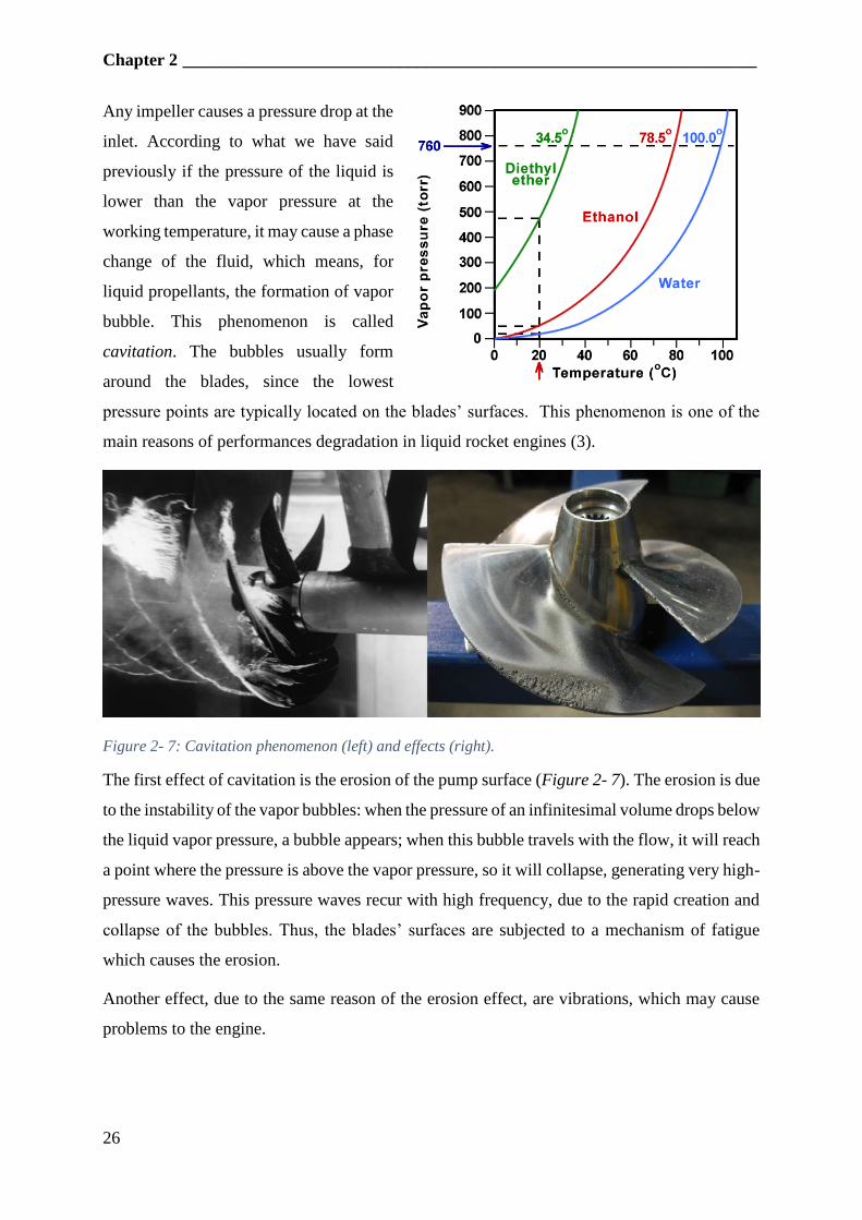
Any impeller causes a pressure drop at the

inlet. According to what we have said

previously if the pressure of the liquid is

lower than the vapor pressure at the

working temperature, it may cause a phase

change of the fluid, which means, for

liquid propellants, the formation of vapor

bubble. This phenomenon is called

cavitation. The bubbles usually form

around the blades, since the lowest

pressure points are typically located on the blades’ surfaces. This phenomenon is one of the

main reasons of performances degradation in liquid rocket engines (3).

Figure 2- 7: Cavitation phenomenon (left) and effects (right).

The first effect of cavitation is the erosion of the pump surface (Figure 2- 7). The erosion is due

to the instability of the vapor bubbles: when the pressure of an infinitesimal volume drops below

the liquid vapor pressure, a bubble appears; when this bubble travels with the flow, it will reach

a point where the pressure is above the vapor pressure, so it will collapse, generating very high-

pressure waves. This pressure waves recur with high frequency, due to the rapid creation and

collapse of the bubbles. Thus, the blades’ surfaces are subjected to a mechanism of fatigue

which causes the erosion.

Another effect, due to the same reason of the erosion effect, are vibrations, which may cause

problems to the engine.

Figure 2- 6

_________________________________________________________ 2.4 Pump parameters

27

The last effect considered is the instability of the volumetric flow, due to the increase of volume

caused by the bubbles formation. This phenomenon may cause non-optimal combustion and

reduce the thrust.

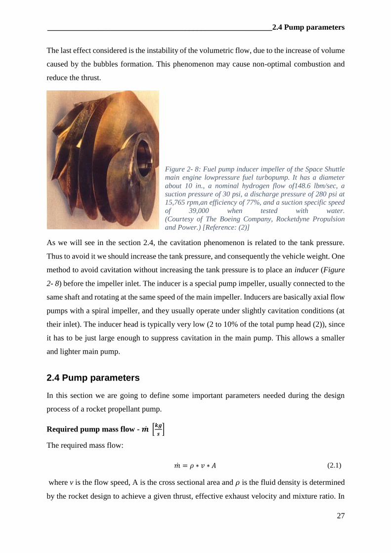
Figure 2- 8: Fuel pump inducer impeller of the Space Shuttle

main engine lowpressure fuel turbopump. It has a diameter

about 10 in., a nominal hydrogen flow of148.6 lbm/sec, a

suction pressure of 30 psi, a discharge pressure of 280 psi at

15,765 rpm,an efficiency of 77%, and a suction specific speed

of 39,000 when tested with water.

(Courtesy of The Boeing Company, Rocketdyne Propulsion

and Power.) [Reference: (2)]

As we will see in the section 2.4, the cavitation phenomenon is related to the tank pressure.

Thus to avoid it we should increase the tank pressure, and consequently the vehicle weight. One

method to avoid cavitation without increasing the tank pressure is to place an inducer (Figure

2- 8) before the impeller inlet. The inducer is a special pump impeller, usually connected to the

same shaft and rotating at the same speed of the main impeller. Inducers are basically axial flow

pumps with a spiral impeller, and they usually operate under slightly cavitation conditions (at

their inlet). The inducer head is typically very low (2 to 10% of the total pump head (2)), since

it has to be just large enough to suppress cavitation in the main pump. This allows a smaller

and lighter main pump.

2.4 Pump parameters

In this section we are going to define some important parameters needed during the design

process of a rocket propellant pump.

Required pump mass flow - 𝒎 [𝒌𝒈

𝒔]

The required mass flow:

where v is the flow speed, A is the cross sectional area and 𝜌 is the fluid density is determined

by the rocket design to achieve a given thrust, effective exhaust velocity and mixture ratio. In

�� = 𝜌 ∗ 𝑣 ∗ 𝐴 (2.1)

Chapter 2 __________________________________________________________________

28

addition to the flow required by the combustion chamber, if part of the flow bypasses the pump,

it has also to be accounted for.

The product v*A is defined as volumetric flow rate Q [𝑚3

𝑠] and can be determined by one of the

two relations presents in Equation (2.2).

𝑄 = 𝑣 ∗ 𝐴 = 𝑚

𝜌

(2.2)

Mixture ratio - 𝜶

The mass flow (as well as the volumetric flow rate) represent the total flow of propellant, so it

is important to know the mixture ratio between fuel and oxidizer. The mixture ratio is defined

as the oxidizer mass flow divided by the fuel mass flow, as shown by equation (2.3).

𝛼 = 𝑚𝑜

𝑚𝑓 (2.3)

For RP-1/LOX it usually ranges between 2.2 and 3, for Hydrogen/LOX has values between 5

and 7.

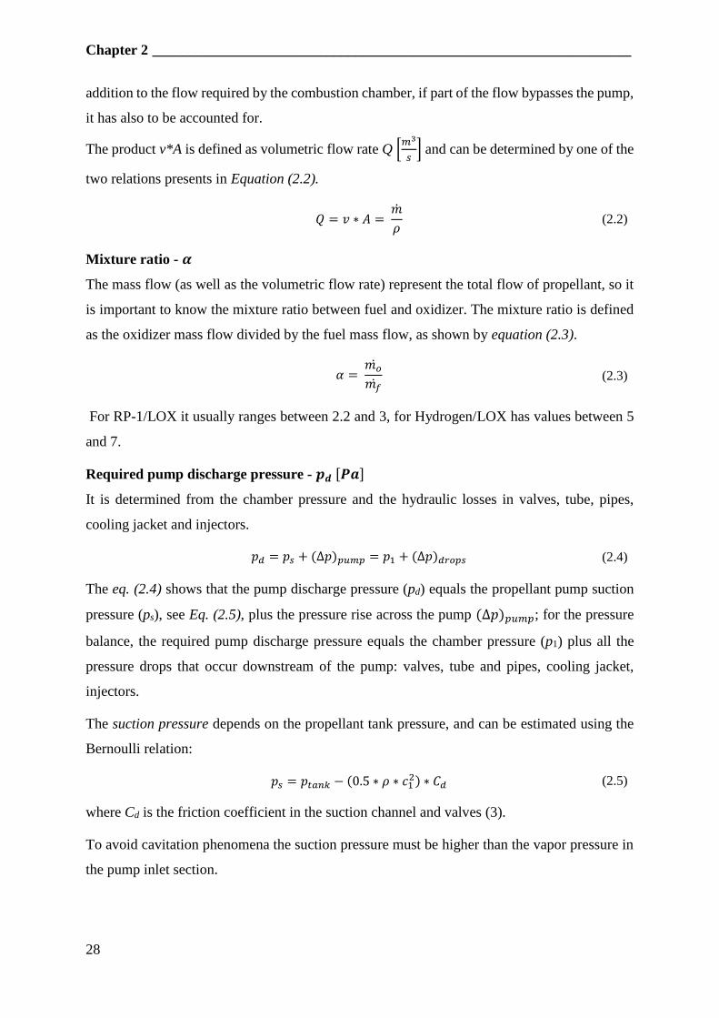
Required pump discharge pressure - 𝒑𝒅 [𝑷𝒂]

It is determined from the chamber pressure and the hydraulic losses in valves, tube, pipes,

cooling jacket and injectors.

𝑝𝑑 = 𝑝𝑠 + (Δ𝑝)𝑝𝑢𝑚𝑝 = 𝑝1 + (Δ𝑝)𝑑𝑟𝑜𝑝𝑠 (2.4)

The eq. (2.4) shows that the pump discharge pressure (pd) equals the propellant pump suction

pressure (ps), see Eq. (2.5), plus the pressure rise across the pump (Δ𝑝)𝑝𝑢𝑚𝑝; for the pressure

balance, the required pump discharge pressure equals the chamber pressure (p1) plus all the

pressure drops that occur downstream of the pump: valves, tube and pipes, cooling jacket,

injectors.

The suction pressure depends on the propellant tank pressure, and can be estimated using the

Bernoulli relation:

𝑝𝑠 = 𝑝𝑡𝑎𝑛𝑘 − (0.5 ∗ 𝜌 ∗ 𝑐12) ∗ 𝐶𝑑 (2.5)

where Cd is the friction coefficient in the suction channel and valves (3).

To avoid cavitation phenomena the suction pressure must be higher than the vapor pressure in

the pump inlet section.

_________________________________________________________ 2.4 Pump parameters

29

Manometric head - H [m]

The Manometric head represent the pressure increase generated by the pump between discharge

and suction. It can be expressed as

∆𝐻 =𝑝𝑑−𝑝𝑠

𝜌 ∗ 𝑔+ 𝑌𝑠 + 𝑌𝑑 (2.6)

where Ys and Yd are the friction losses in the channels before and after the pump

Net positive suction head – NPSH [m]

The NPSH can be divided into two type: the required NPSH (NPSHr) and the available NPSH

(NPSHa). Both are pressure measurement expressed in meters.

The NPSHr is the limit value of the head at the pump inlet that allows to avoid cavitation

phenomena (see section 2.1.1). It is necessary to have this pressure at the inlet because every

pump generates a pressure drop at the entrance of the impeller vanes. Therefore, all pump

systems must maintain a positive suction pressure to overcome this pressure drop. The NPSHr

depends upon the pump design and the working-fluid.

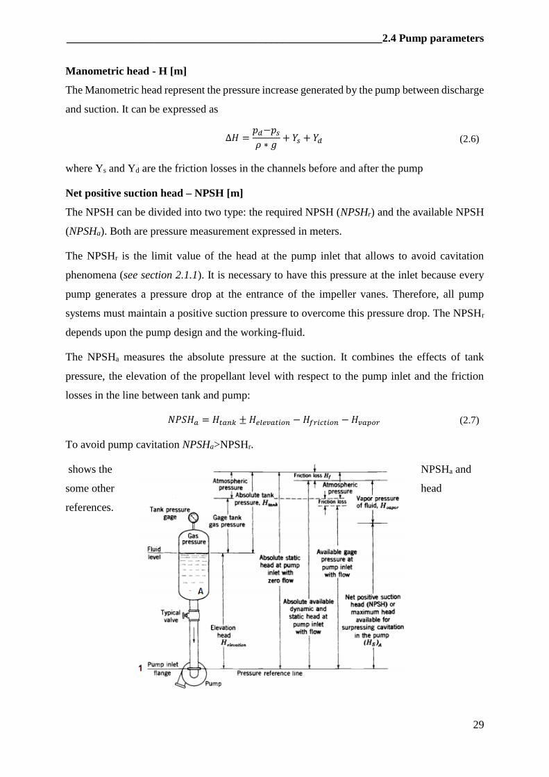
The NPSHa measures the absolute pressure at the suction. It combines the effects of tank

pressure, the elevation of the propellant level with respect to the pump inlet and the friction

losses in the line between tank and pump:

𝑁𝑃𝑆𝐻𝑎 = 𝐻𝑡𝑎𝑛𝑘 ± 𝐻𝑒𝑙𝑒𝑣𝑎𝑡𝑖𝑜𝑛 − 𝐻𝑓𝑟𝑖𝑐𝑡𝑖𝑜𝑛 − 𝐻𝑣𝑎𝑝𝑜𝑟 (2.7)

To avoid pump cavitation NPSHa>NPSHr.

shows the NPSHa and

some other head

references.

Chapter 2 __________________________________________________________________

30

Let us make some

consideration in order to determine the NPSH from a theoretical point of view.

By applying the generalized Bernoulli’s equation between the tank and the pump inlet (which

is the point of minimum pressure) we obtain:

−𝐿𝑤 =𝑝1 − 𝑝𝐴

𝜌+

𝑐12

2+ 𝑔(𝑧1 − 𝑧𝐴) (2.8)

In writing Eq. (2.8) we have neglected the fluid velocity in the tank and we have used Lw to

denote the head loss that occurs in the line between tank and pump.

Calling Helev = g(z1-za) the fluid level – pump inlet head, we can rearrange the Equation (2.8)

as:

𝑝1 = 𝑝𝐴 − 𝛾𝐿𝑤 − 𝜌𝑐1

2

2− 𝛾𝐻𝑒𝑙𝑒𝑣 (2.9)

where γ = ρ*g is the specific weight, defined as weight per unit of volume [N/m3].

If we want to be more accurate, we should consider that around the impeller blades there are

some areas where pressure is lower than p1. To account for this, we can subtract a ∆p to the p1,

obtaining equation (2.10).

𝑝1 = 𝑝𝐴 − 𝛾𝐿𝑤 − 𝜌𝑐1

2

2− 𝛾𝐻𝑒𝑙𝑒𝑣 − Δ𝑝 (2.10)

To avoid cavitation, the pressure at the pump inlet p1 must be higher than the vapor pressure pv

of the fluid at the fluid temperature.

We can rearrange the equation (2.10) into equation (2.11) by separating the system

characteristic (NPSHa) from the pump characteristic (NPSHr)

𝑁𝑃𝑆𝐻𝑎 =𝑝𝐴 − 𝑝𝑣

𝛾− 𝐿𝑤 − 𝐻𝑒𝑙𝑒𝑣 >

𝜌𝑐12

2𝛾+

Δ𝑝

𝛾= 𝑁𝑃𝑆𝐻𝑟 (2.11)

Suction specific speed – S

The suction specific speed can be defined by the equation (2.12), where Nr is the number of

revolutions per seconds, or by the equation (2.13), where ω is the angular velocity expressed in

radians per seconds.

𝑆 =𝑁𝑟√𝑄

(𝑔 ∗ 𝑁𝑃𝑆𝐻𝑟)3/4 (2.12)

Figure 2- 9 Definition of pump net positive suction

_________________________________________________________ 2.4 Pump parameters

31

𝑆 =𝜔√𝑄

(𝑔 ∗ 𝑁𝑃𝑆𝐻𝑟)3/4 (2.13)

When using the number of revolutions per second, the suction specific speed ranges between

1.8 and 2.4 for axial turbopumps, and between 2.5 and 3 for centrifugal turbopumps (3).

When using the angular velocity S ranges between 14 and 24.

In both equations (2.12) and (2.13) NPSHr is the required net positive suction head, therefore

knowing the suction specific speed, the volumetric flow and the impeller speed, we can

determine the NPSHr.

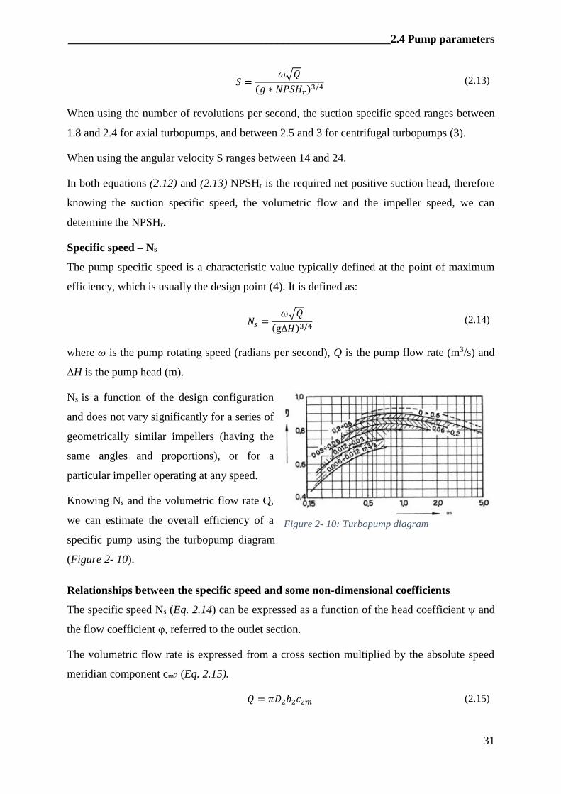
Specific speed – Ns

The pump specific speed is a characteristic value typically defined at the point of maximum

efficiency, which is usually the design point (4). It is defined as:

𝑁𝑠 =𝜔√𝑄

(gΔ𝐻)3/4 (2.14)

where ω is the pump rotating speed (radians per second), Q is the pump flow rate (m3/s) and

∆H is the pump head (m).

Ns is a function of the design configuration

and does not vary significantly for a series of

geometrically similar impellers (having the

same angles and proportions), or for a

particular impeller operating at any speed.

Knowing Ns and the volumetric flow rate Q,

we can estimate the overall efficiency of a

specific pump using the turbopump diagram

(Figure 2- 10).

Relationships between the specific speed and some non-dimensional coefficients

The specific speed Ns (Eq. 2.14) can be expressed as a function of the head coefficient ψ and

the flow coefficient φ, referred to the outlet section.

The volumetric flow rate is expressed from a cross section multiplied by the absolute speed

meridian component cm2 (Eq. 2.15).

𝑄 = 𝜋𝐷2𝑏2𝑐2𝑚 (2.15)

Figure 2- 10: Turbopump diagram

Chapter 2 __________________________________________________________________

32

The discharge flow coefficient is defined as:

𝜑2 =𝑐2𝑚

𝑢2 (2.16)

We can replace 𝑐𝑚2 in the Eq. (2.15) with a function of 𝜑 and 𝑢2:

𝑄 = 𝜑𝜋𝐷2𝑏2𝑢2 (2.17)

Replacing Equation (2.17) into Equation (2.14) we obtain

𝑁𝑠 =𝜔√𝜑𝜋𝐷2𝑏2𝑢2

(𝑔Δ𝐻)3/4 (2.18)

The angular velocity ω can be written as:

𝜔 =2 ∗ 𝑢2

𝐷2 (2.19)

Substituting the (2.19) in the (2.18) we obtain Equation (2.20).

𝑁𝑠 =2√𝜋𝐷2𝑏2

𝐷2

𝑢23/2

(𝑔Δ𝐻)3/4𝜙1/2 = 2√𝜋√

𝑏2

𝐷2(

𝑢22

𝑔Δ𝐻)

3/4

𝜑1/2 (2.20)

By definition, the head coefficient equals to:

𝜓 =𝑔Δ𝐻

𝑢22 (2.21)

Substituting the (2.21) into the (2.20) we obtain:

𝑁𝑠 = 2√𝜋√𝑏2

𝐷2

𝜑1/2

𝜓3/4 (2.22)

Equation (2.22) express the specific speed as a function of the ratio 𝑏2

𝐷2 and the flow and head

coefficients.

For pumps typically used for liquid rocket engines, the values of flow coefficients are:

- Inlet flow coefficient (𝑢𝑒= impeller eye velocity):

- Discharge flow coefficient (𝑢2=impeller tip speed, usually between 182.88 and 609.6

[m/s])

𝜑1

=𝑐1𝑚

𝑢𝑒

= 0.08 ÷ 0.4 (2.23)

𝜑2 =𝑐2𝑚

𝑢2= 0.05 ÷ 0.3 (2.24)

_________________________________________________________ 2.4 Pump parameters

33

The discharge meridian velocity 𝑐𝑚2 should be approximately 1.5 times higher than the inlet

meridian velocity 𝑐𝑚1.

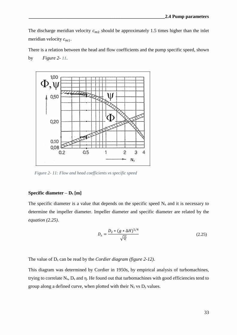
There is a relation between the head and flow coefficients and the pump specific speed, shown

by Figure 2- 11.

Figure 2- 11: Flow and head coefficients vs specific speed

Specific diameter – Ds [m]

The specific diameter is a value that depends on the specific speed Ns and it is necessary to

determine the impeller diameter. Impeller diameter and specific diameter are related by the

equation (2.25).

𝐷𝑠 =𝐷2 ∗ (𝑔 ∗ Δ𝐻)1/4

√𝑄 (2.25)

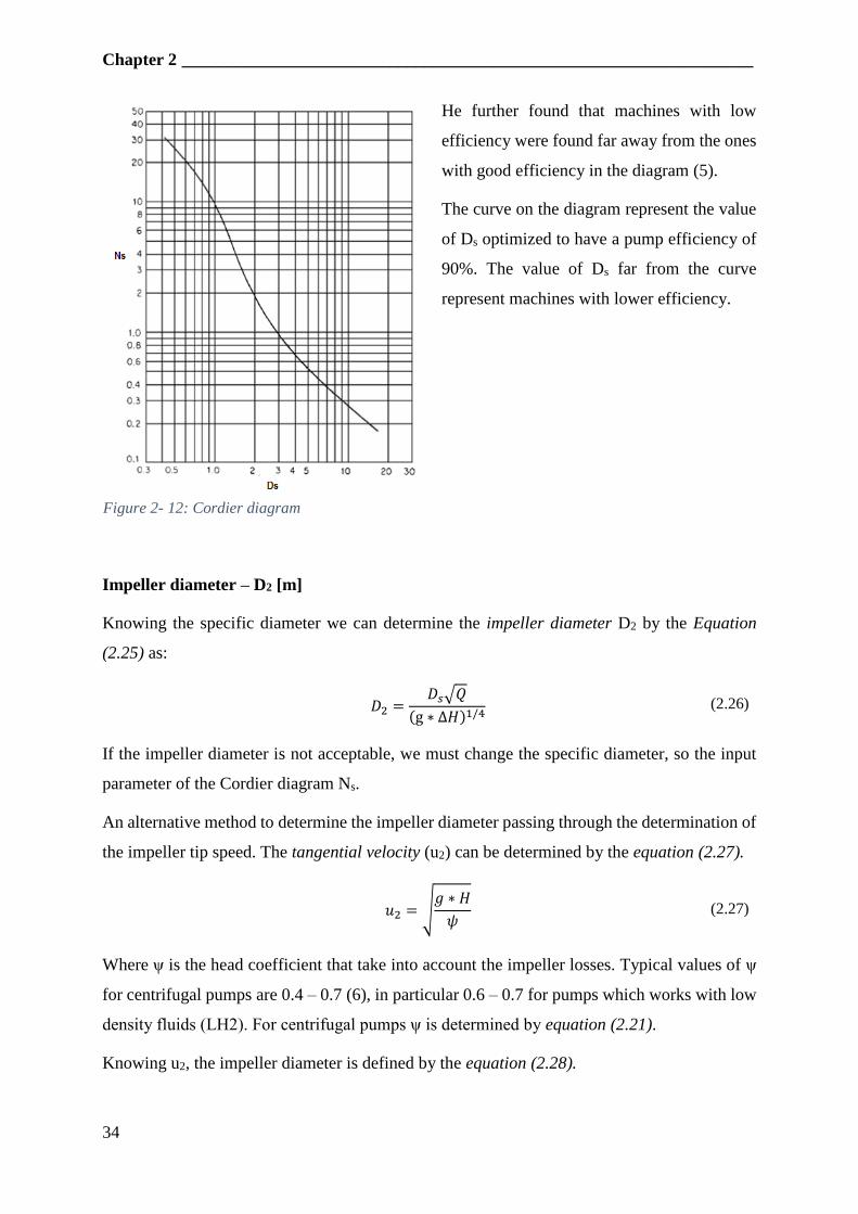
The value of Ds can be read by the Cordier diagram (figure 2-12).

This diagram was determined by Cordier in 1950s, by empirical analysis of turbomachines,

trying to correlate Ns, Ds and η. He found out that turbomachines with good efficiencies tend to

group along a defined curve, when plotted with their Ns vs Ds values.

Chapter 2 __________________________________________________________________

34

He further found that machines with low

efficiency were found far away from the ones

with good efficiency in the diagram (5).

The curve on the diagram represent the value

of Ds optimized to have a pump efficiency of

90%. The value of Ds far from the curve

represent machines with lower efficiency.

Impeller diameter – D2 [m]

Knowing the specific diameter we can determine the impeller diameter D2 by the Equation

(2.25) as:

𝐷2 =𝐷𝑠√𝑄

(g ∗ Δ𝐻)1/4 (2.26)

If the impeller diameter is not acceptable, we must change the specific diameter, so the input

parameter of the Cordier diagram Ns.

An alternative method to determine the impeller diameter passing through the determination of

the impeller tip speed. The tangential velocity (u2) can be determined by the equation (2.27).

𝑢2 = √𝑔 ∗ 𝐻

𝜓 (2.27)

Where ψ is the head coefficient that take into account the impeller losses. Typical values of ψ

for centrifugal pumps are 0.4 – 0.7 (6), in particular 0.6 – 0.7 for pumps which works with low

density fluids (LH2). For centrifugal pumps ψ is determined by equation (2.21).

Knowing u2, the impeller diameter is defined by the equation (2.28).

Figure 2- 12: Cordier diagram

_________________________________________________________ 2.4 Pump parameters

35

𝐷2 =2 ∗ 𝑢2

𝜔 (2.28)

The impeller speed is limited by the design material strength to about 610 m/s. With titanium

(lower density than steel) and machined cantilevered impellers a speed of over 655 m/s (2). For

cast impellers this limiting value is lower than for machined impellers. Consequently, once we

have determined the impeller diameter and velocity, we have to verify if the stress acting on the

impeller is lower than the material admissible stress.

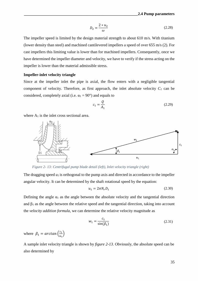
Impeller-inlet velocity triangle

Since at the impeller inlet the pipe is axial, the flow enters with a negligible tangential

component of velocity. Therefore, as first approach, the inlet absolute velocity C1 can be

considered, completely axial (i.e. α1 = 90°) and equals to

𝑐1 =𝑄

𝐴1 (2.29)

where A1 is the inlet cross sectional area.

The dragging speed u1 is orthogonal to the pump axis and directed in accordance to the impeller

angular velocity. It can be determined by the shaft rotational speed by the equation:

𝑢1 = 2𝜋𝑁𝑟𝐷1 (2.30)

Defining the angle α1 as the angle between the absolute velocity and the tangential direction

and β1 as the angle between the relative speed and the tangential direction, taking into account

the velocity addition formula, we can determine the relative velocity magnitude as

𝑤1 =𝑐1

sin (𝛽1) (2.31)

where 𝛽1 = 𝑎𝑟𝑐𝑡𝑎𝑛 (𝑐1

𝑢1)

A sample inlet velocity triangle is shown by figure 2-13. Obviously, the absolute speed can be

also determined by

Figure 2- 13: Centrifugal pump blade detail (left), Inlet velocity triangle (right)

Chapter 2 __________________________________________________________________

36

𝑐1 = 𝑢1 ∗ tan (𝛽1) (2.32)

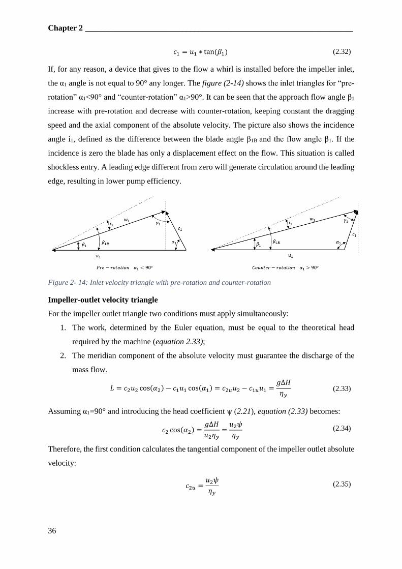
If, for any reason, a device that gives to the flow a whirl is installed before the impeller inlet,

the α1 angle is not equal to 90° any longer. The figure (2-14) shows the inlet triangles for “pre-

rotation” α1<90° and “counter-rotation” α1>90°. It can be seen that the approach flow angle β1

increase with pre-rotation and decrease with counter-rotation, keeping constant the dragging

speed and the axial component of the absolute velocity. The picture also shows the incidence

angle i1, defined as the difference between the blade angle β1B and the flow angle β1. If the

incidence is zero the blade has only a displacement effect on the flow. This situation is called

shockless entry. A leading edge different from zero will generate circulation around the leading

edge, resulting in lower pump efficiency.

Figure 2- 14: Inlet velocity triangle with pre-rotation and counter-rotation

Impeller-outlet velocity triangle

For the impeller outlet triangle two conditions must apply simultaneously:

1. The work, determined by the Euler equation, must be equal to the theoretical head

required by the machine (equation 2.33);

2. The meridian component of the absolute velocity must guarantee the discharge of the

mass flow.

𝐿 = 𝑐2𝑢2 cos(𝛼2) − 𝑐1𝑢1 cos(𝛼1) = 𝑐2𝑢𝑢2 − 𝑐1𝑢𝑢1 =𝑔Δ𝐻

𝜂𝑦 (2.33)

Assuming α1=90° and introducing the head coefficient ψ (2.21), equation (2.33) becomes:

𝑐2 cos(𝛼2) =𝑔Δ𝐻

𝑢2𝜂𝑦=

𝑢2𝜓

𝜂𝑦 (2.34)

Therefore, the first condition calculates the tangential component of the impeller outlet absolute

velocity:

𝑐2𝑢 =𝑢2𝜓

𝜂𝑦 (2.35)

_________________________________________________________ 2.4 Pump parameters

37

The second condition, under the assumption of uniform speed on the cross section at the

impeller outlet, immediately defines the meridian component of the absolute velocity (2.36),

directly from the definition of flow coefficient (2.16)

𝑐2𝑚 = 𝜑 ∗ 𝑢2 (2.36)

Being known the absolute speed components, it is possible to determine the absolute speed

magnitude (2.37)

𝑐2 = √𝑐2𝑚2 + 𝑐2𝑢

2 (2.37)

The angle β2 can be determined by:

𝛽2 = 𝑎𝑟𝑐𝑡𝑎𝑛 (𝑐2𝑚

𝑢2 − 𝑐2𝑢) (2.38)

The tangent of α2 equals to:

tan (𝛼2) =𝑐2𝑚

𝑐2𝑢=

𝜑 ∗ 𝑢2

𝜓 ∗ 𝑢2𝜂𝑦

=𝜑

𝜓𝜂𝑦

(2.39)

Therefore

𝛼2 = arctan (𝑐𝑚2

𝑐𝑢2) = 𝑎𝑟𝑐𝑡𝑎𝑛 (

𝜑

𝜓𝜂𝑦

) (2.40)

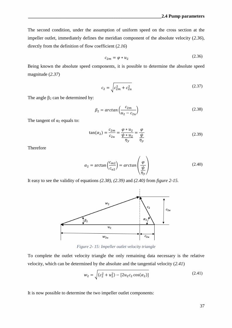
It easy to see the validity of equations (2.38), (2.39) and (2.40) from figure 2-15.

Figure 2- 15: Impeller outlet velocity triangle

To complete the outlet velocity triangle the only remaining data necessary is the relative

velocity, which can be determined by the absolute and the tangential velocity (2.41)

𝑤2 = √(𝑐22 + 𝑢2

2) − [2𝑢2𝑐2 cos(𝛼2)] (2.41)

It is now possible to determine the two impeller outlet components:

Chapter 2 __________________________________________________________________

38

- The meridian component w2m coincides with c2m

𝑤2𝑚 = 𝑐2𝑚 = 𝑤2sin (𝛼2) (2.42)

- The tangential component w2u

𝑤2𝑢 = 𝑤2cos (𝛼2) (2.43)

or

𝑤2𝑢 = 𝑢2 − 𝑐2𝑢 = 𝑢2 − 𝑐2cos (𝛼2) (2.44)

Another relation to determine the β2 angle is:

β2 = 𝑎𝑟𝑐𝑡𝑎𝑛 (𝑤2𝑚

𝑤2𝑢) (2.45)

Since the relative speed w2 is inclined at the angle β2, it can be written as

𝑤2 =𝑢2 − 𝑐2𝑢

cos (𝛽2) (2.46)

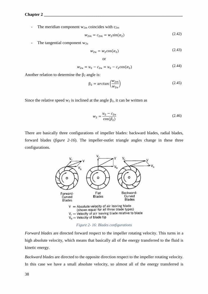
There are basically three configurations of impeller blades: backward blades, radial blades,

forward blades (figure 2-16). The impeller-outlet triangle angles change in these three

configurations.

Figure 2- 16: Blades configurations

Forward blades are directed forward respect to the impeller rotating velocity. This turns in a

high absolute velocity, which means that basically all of the energy transferred to the fluid is

kinetic energy.

Backward blades are directed to the opposite direction respect to the impeller rotating velocity.

In this case we have a small absolute velocity, so almost all of the energy transferred is

_________________________________________________________ 2.4 Pump parameters

39

transformed in pressure. Backward-blades impeller are more often used, because they have a

higher efficiency and prevent boundary layer separation.

Blade numbers - z

The number of blades (z) needed to have an efficient impeller can be estimated by a simple

empirical relation (3)

𝑧 = 2 ∗ 𝑘 ∗𝑅𝑠

𝑙𝑏∗ sin (𝛽𝑚) (2.47)

Where lb is the blades length expressed in meters (2.48), Rs is the mean radius expressed in

meters (2.49), βm is the average angle (2.50) and k is a coefficient that depends on the pump

architecture (k=6.5 for centrifugal pumps; k=4.5 for axial pumps).

𝑙𝑏 =𝐷2 − 𝐷1

2 (2.48)

𝑅𝑠 =

𝐷2 + 𝐷1

4

(2.49)

𝛽𝑚 =

𝛽1 + 𝛽2

2

(2.50)

Total pump efficiency - 𝜼𝒑

The total efficiency of a pump can be seen as the product of three efficiencies (2.51):

𝜂𝑝 = 𝜂𝑦𝜂𝑣𝜂𝑇𝑟 (2.51)

- 𝜂𝑦 hydraulic efficiency. The hydraulic efficiency depends on the specific speed and on

the machine architecture. It also depends on the Reynolds number and on the roughness

of the impeller surface. [Typical values between 0.7 and 0.96].

- 𝜂𝑣 volumetric efficiency. The volumetric efficiency is defined as the ratio of the outlet

flow rate delivered by the pump and the theoretical discharge flow rate produced by the

pump (i.e. the inlet flow rate). It gives an esteem of the flow loss due to leakage of the

fluid through the pump. [Typical values between 0.85 and 0.97]

- 𝜂𝑇𝑟 transmission efficiency. The transmission efficiency considers the losses between

the pump and the turbine, due to bearings, gears and any other moving part. [Typical

values between 0.88 and 0.97]

Chapter 2 __________________________________________________________________

40

2.5 Pump design methods

2.5.1 Method 1

The input parameter is the number of rotation per minute Nr [rpm]. The choice of Nr depends

on the propellant density.

The first step is calculate the angular velocity ω[𝑟𝑎𝑑

𝑠], as shown by equation (2.52).

ω =2 ∗ 𝜋 ∗ 𝑛

60 (2.52)

Then we calculate the volumetric flow rate Q and the head H.

It is now possible to calculate the specific speed Ns, consequently it is possible to read on the

Cordier diagram the specific diameter Ds that makes the pump work with a good efficiency.

From the specific diameter we can calculate the outlet diameter D2

𝐷2 =𝐷𝑠√𝑄

(g ∗ Δ𝐻)1/4 (2.53)

Knowing the outlet diameter the impeller tip speed is equal to

𝑢2 =𝐷2 ∗ 𝑁0

2 (2.54)

The power absorbed [W] by the pumps is determined by equations (2.55) and (2.56)

respectively for oxidizer and fuel pump.

(𝑃𝑎)𝑜𝑥 =(��)𝑜𝑥 ∗ [(𝑝𝑑)𝑜𝑥 − (𝑝𝑠)𝑜𝑥]

𝜌𝑜𝑥 ∗ 𝜂𝑜𝑥 (2.55)

(𝑃𝑎)𝑓 =(��)𝑓 ∗ [(𝑝𝑑)𝑓 − (𝑝𝑠)𝑓]

𝜌𝑓 ∗ 𝜂𝑓 (2.56)

Knowing the suction specific speed S we can determine the required NPSHr [m] by the equation

(2.57), which directly comes from eq. (2.13).

𝑁𝑃𝑆𝐻𝑟 =

1

(𝑔 ∗𝑆

ω ∗ 𝑄0.5)1.33

(2.57)

- S = 1.8 ~ 2.3 Axial turbopumps;

- S = 2.5 ~ 3 Radial turbopumps;

While the NPSHa [m] is equals to

_____________________________________________________ 2.5 Pump design methods

41

𝑁𝑃𝑆𝐻𝑎 =𝑝𝑠 − 𝑝𝑣

𝜌 ∗ 𝑔 (2.58)

2.5.2 Method 2

The input parameters are: volumetric flow Q, Manometric head H, specific speed Ns, suction

specific speed S.

The first step is to calculate the specific angular velocity ω

ω =𝑁𝑠 ∗ (𝑔 ∗ 𝐻)3/4

√𝑄 (2.59)

The impeller tip speed u2 [m/s] is obtained by the pump coefficient ψ

𝑢2 = √𝑔 ∗ 𝐻

𝜓 (2.60

The cavitation verification is the same as the previous method. In this case

𝑁𝑃𝑆𝐻𝑟 =

1

(𝑔 ∗𝑆

𝑁0𝑠 ∗ 𝑄0.5)1.33

(2.61)

Where S = 15~24

𝑆 =𝑁0𝑠 ∗ √𝑄

(𝑔 ∗ 𝑁𝑃𝑆𝐻𝑟)3/4 (2.62)

The suction diameter (in meters) can be calculated by equation (2.63).

𝐷1 = (

8𝑄𝜋⁄

𝜑𝑖𝑛 ∗ 𝑁0𝑠 ∗ (1 − 𝜈2))

1/3

(2.63)

Where

- φin= flow coefficient, generally equals to 0.1 for the suction section

- ν = shaft diameter – suction diameter ratio, usually between 0.20 and 0.35

The powers can be calculated by [W]

(𝑃𝑎)𝑜𝑥 =��𝑜𝑥 ∗ 𝑔 ∗ 𝐻𝑜𝑥

𝜂𝑜𝑥 (2.64)

(𝑃𝑎)𝑓 =��𝑓 ∗ 𝑔 ∗ 𝐻𝑓

𝜂𝑓 (2.65)

Respectively for oxidizer and fuel pump.

Chapter 2 __________________________________________________________________

42

2.5.3 Method 3

The input parameter are: volumetric flow Q, manometric head H, specific speed Ns, suction

channel diameter D.

The angular velocity ω [rad/s] is equal to

𝜔 =𝑁𝑠 ∗ (𝑔 ∗ 𝐻)3/4

√𝑄 (2.66)

The absolute speed at the inlet section of the pump c1 [m/s] is

𝑐1 =4 ∗ 𝑄

𝜋 ∗ 𝐷2 (2.67)

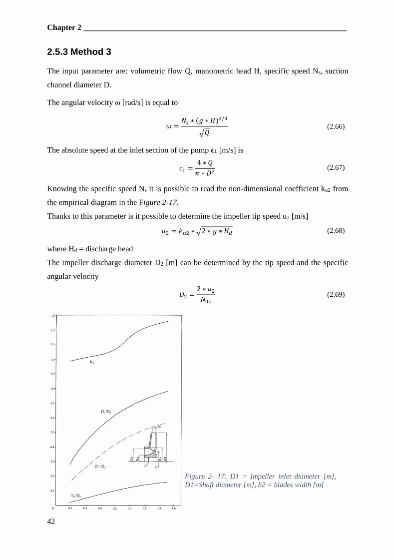
Knowing the specific speed Ns it is possible to read the non-dimensional coefficient ku2 from

the empirical diagram in the Figure 2-17.

Thanks to this parameter is it possible to determine the impeller tip speed u2 [m/s]

𝑢2 = 𝑘𝑢2 ∗ √2 ∗ 𝑔 ∗ 𝐻𝑑 (2.68)

where Hd = discharge head

The impeller discharge diameter D2 [m] can be determined by the tip speed and the specific

angular velocity

𝐷2 =2 ∗ 𝑢2

𝑁0𝑠 (2.69)

Figure 2- 17: D1 = Impeller inlet diameter [m],

D1=Shaft diameter [m], b2 = blades width [m]

____________________________________________________________ 2.6 Volute design

43

To determine the blade outlet angle we prescribe:

- ηv = volumetric efficiency (between 0.90 and 0.97)

- ψ2 = adimensional coefficient which consider blades volume, generally equal to 0.95

The discharge speed c2 [m/s] is equal to

𝑐2 =𝑄

𝜋 ∗ 𝐷2 ∗ 𝑏2 ∗ 𝜓2 ∗ 𝜂𝑣 (2.70)

In conclusion the outlet blades β2 angle can be determined by equation (2.71).

𝛽2 = 𝐴𝑟𝑐𝐶𝑜𝑡 (𝑢2 − 𝑣2𝑡

𝑐2) (2.71)

where

𝑣2𝑡 =𝑔 ∗ 𝐻𝑑

𝑢2 ∗ 𝜂𝑦 (2.72)

ηy = hydraulic efficiency (0.7~0.96 for rocket engines turbopumps).

2.6 Volute design

There are several possible volute shape design. The most common are:

- Spiral volute: is the first type of volute used on centrifugal pumps. Volute casing of

constant velocity of this type are simple to design and more economical to produce

because of the open areas around the impeller periphery. They can be used on large as

well as small pumps of all specific speeds with good efficiency.

- Double volute: consists of two opposed single volute. The total throat area is the same

as the one that would be used on a comparable single volute. The hydraulic performance

is comparable to the single volute design. Tests indicate that a double volute pump will

be less efficient at the best efficiency point with respect to a single spiral volute, but

more efficient on both sides of the best efficiency point respect a single spiral volute.

Double volute should not be used in low flow pumps, because the small cross section

makes difficult manufacturing and cleaning.

- Concentric volute: several experimental studies have been carried out on this volute

type. The results have revealed that concentric volutes improve the hydraulic

performances of low head or low specific speed pumps. Specifically, pump efficiency

is improved for pumps with specific speed under 600 m/s. (7)

Chapter 2 __________________________________________________________________

44

2.6.1 Effect of the volute design on efficiency

One of the main challenges for a pump designer is to design an efficient and durable pump.

Mainly two effects have to be taken into account: the force load on the impeller and the

hydraulic efficiency. Too high forces may cause premature failure of bearings or other

components. Low efficiency turns into higher costs in terms of power needed to drive the pump.

Small changes in volute design have been shown to affect one or both force load on the impeller

and hydraulic efficiency (8).

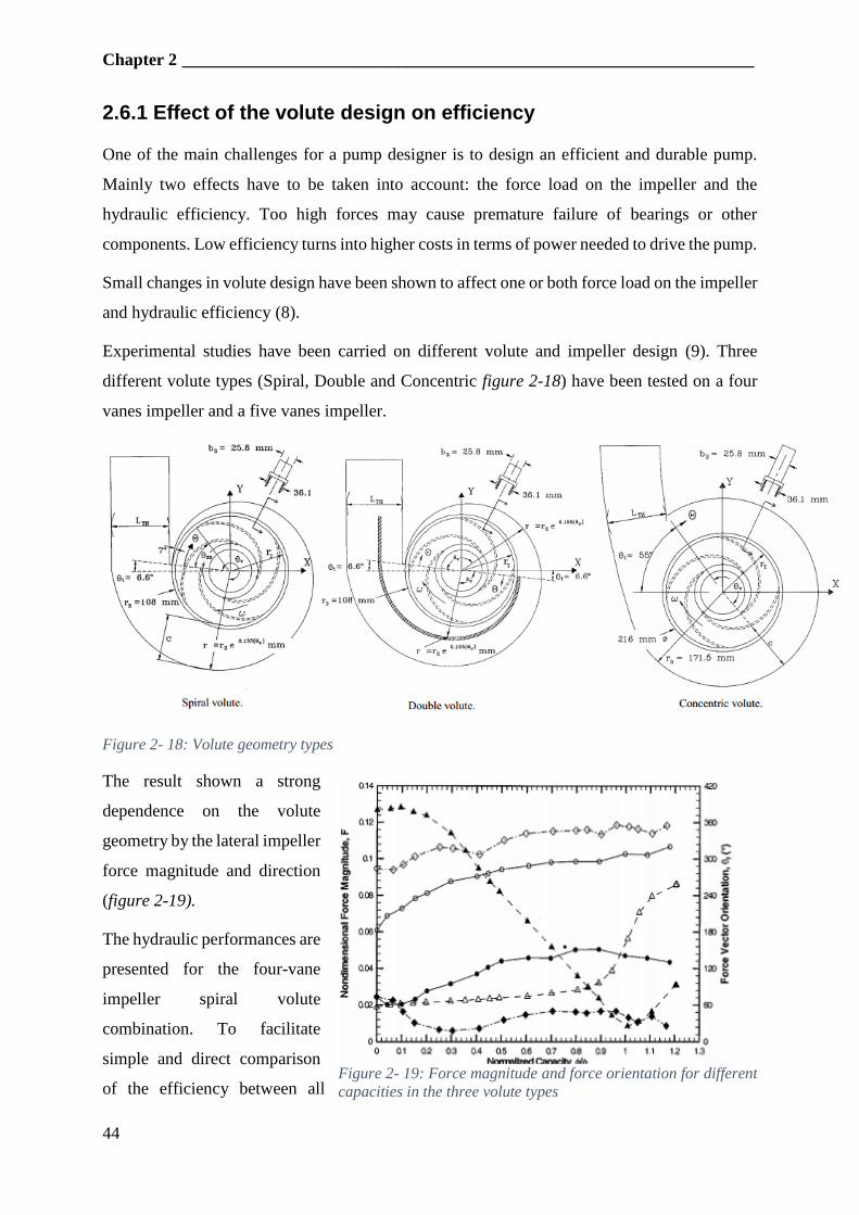
Experimental studies have been carried on different volute and impeller design (9). Three

different volute types (Spiral, Double and Concentric figure 2-18) have been tested on a four

vanes impeller and a five vanes impeller.

Figure 2- 18: Volute geometry types

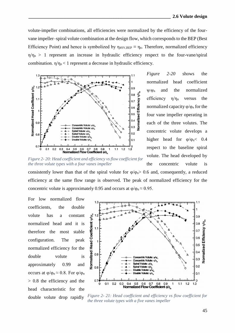
The result shown a strong

dependence on the volute

geometry by the lateral impeller

force magnitude and direction

(figure 2-19).

The hydraulic performances are

presented for the four-vane

impeller spiral volute

combination. To facilitate

simple and direct comparison

of the efficiency between all Figure 2- 19: Force magnitude and force orientation for different

capacities in the three volute types

____________________________________________________________ 2.6 Volute design

45

volute-impeller combinations, all efficiencies were normalized by the efficiency of the four-

vane impeller–spiral volute combination at the design flow, which corresponds to the BEP (Best

Efficiency Point) and hence is symbolized by η4SV,BEP ≡ ηn. Therefore, normalized efficiency

η/ηn > 1 represent an increase in hydraulic efficiency respect to the four-vane/spiral

combination. η/ηn < 1 represent a decrease in hydraulic efficiency.

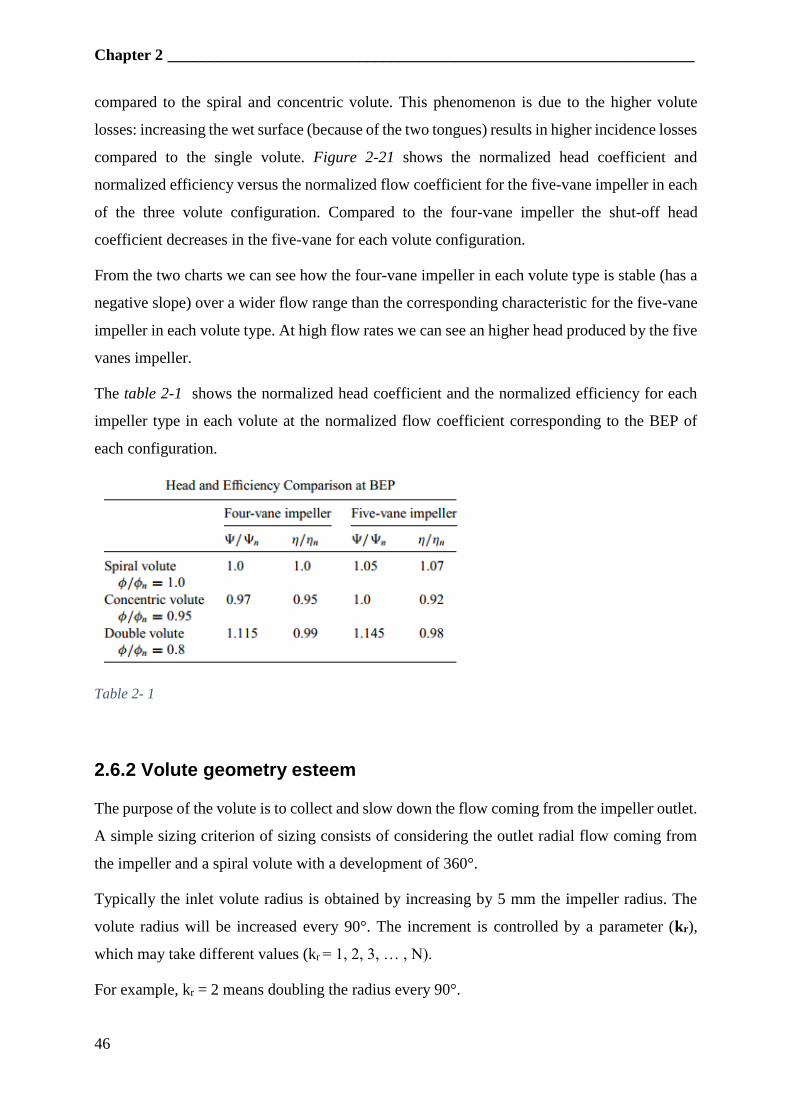
Figure 2-20 shows the

normalized head coefficient

ψ/ψn and the normalized

efficiency η/ηn versus the

normalized capacity φ/φn for the

four vane impeller operating in

each of the three volutes. The

concentric volute develops a

higher head for φ/φn< 0.4

respect to the baseline spiral

volute. The head developed by

the concentric volute is

consistently lower than that of the spiral volute for φ/φn> 0.6 and, consequently, a reduced

efficiency at the same flow range is observed. The peak of normalized efficiency for the

concentric volute is approximately 0.95 and occurs at φ/φn ≈ 0.95.

For low normalized flow

coefficients, the double

volute has a constant

normalized head and it is

therefore the most stable

configuration. The peak

normalized efficiency for the

double volute is

approximately 0.99 and

occurs at φ/φn ≈ 0.8. For φ/φn

> 0.8 the efficiency and the

head characteristic for the

double volute drop rapidly

Figure 2- 20: Head coefficient and efficiency vs flow coefficient for

the three volute types with a four vanes impeller

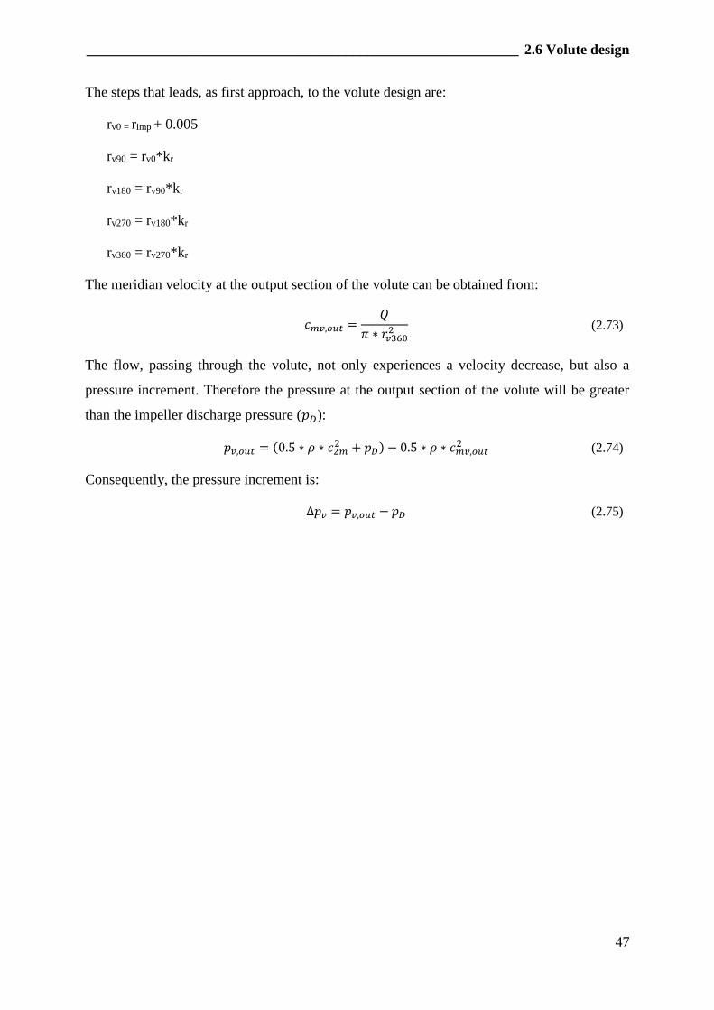
Figure 2- 21: Head coefficient and efficiency vs flow coefficient for

the three volute types with a five vanes impeller

Chapter 2 __________________________________________________________________

46

compared to the spiral and concentric volute. This phenomenon is due to the higher volute

losses: increasing the wet surface (because of the two tongues) results in higher incidence losses

compared to the single volute. Figure 2-21 shows the normalized head coefficient and

normalized efficiency versus the normalized flow coefficient for the five-vane impeller in each

of the three volute configuration. Compared to the four-vane impeller the shut-off head

coefficient decreases in the five-vane for each volute configuration.

From the two charts we can see how the four-vane impeller in each volute type is stable (has a

negative slope) over a wider flow range than the corresponding characteristic for the five-vane

impeller in each volute type. At high flow rates we can see an higher head produced by the five

vanes impeller.

The table 2-1 shows the normalized head coefficient and the normalized efficiency for each

impeller type in each volute at the normalized flow coefficient corresponding to the BEP of

each configuration.

Table 2- 1

2.6.2 Volute geometry esteem

The purpose of the volute is to collect and slow down the flow coming from the impeller outlet.

A simple sizing criterion of sizing consists of considering the outlet radial flow coming from

the impeller and a spiral volute with a development of 360°.

Typically the inlet volute radius is obtained by increasing by 5 mm the impeller radius. The

volute radius will be increased every 90°. The increment is controlled by a parameter (kr),

which may take different values (kr = 1, 2, 3, … , N).

For example, kr = 2 means doubling the radius every 90°.

____________________________________________________________ 2.6 Volute design

47

The steps that leads, as first approach, to the volute design are:

rv0 = rimp + 0.005

rv90 = rv0*kr

rv180 = rv90*kr

rv270 = rv180*kr

rv360 = rv270*kr

The meridian velocity at the output section of the volute can be obtained from:

𝑐𝑚𝑣,𝑜𝑢𝑡 =𝑄

𝜋 ∗ 𝑟𝑣3602 (2.73)

The flow, passing through the volute, not only experiences a velocity decrease, but also a

pressure increment. Therefore the pressure at the output section of the volute will be greater

than the impeller discharge pressure (𝑝𝐷):

𝑝𝑣,𝑜𝑢𝑡 = (0.5 ∗ 𝜌 ∗ 𝑐2𝑚2 + 𝑝𝐷) − 0.5 ∗ 𝜌 ∗ 𝑐𝑚𝑣,𝑜𝑢𝑡

2 (2.74)

Consequently, the pressure increment is:

Δ𝑝𝑣 = 𝑝𝑣,𝑜𝑢𝑡 − 𝑝𝐷 (2.75)

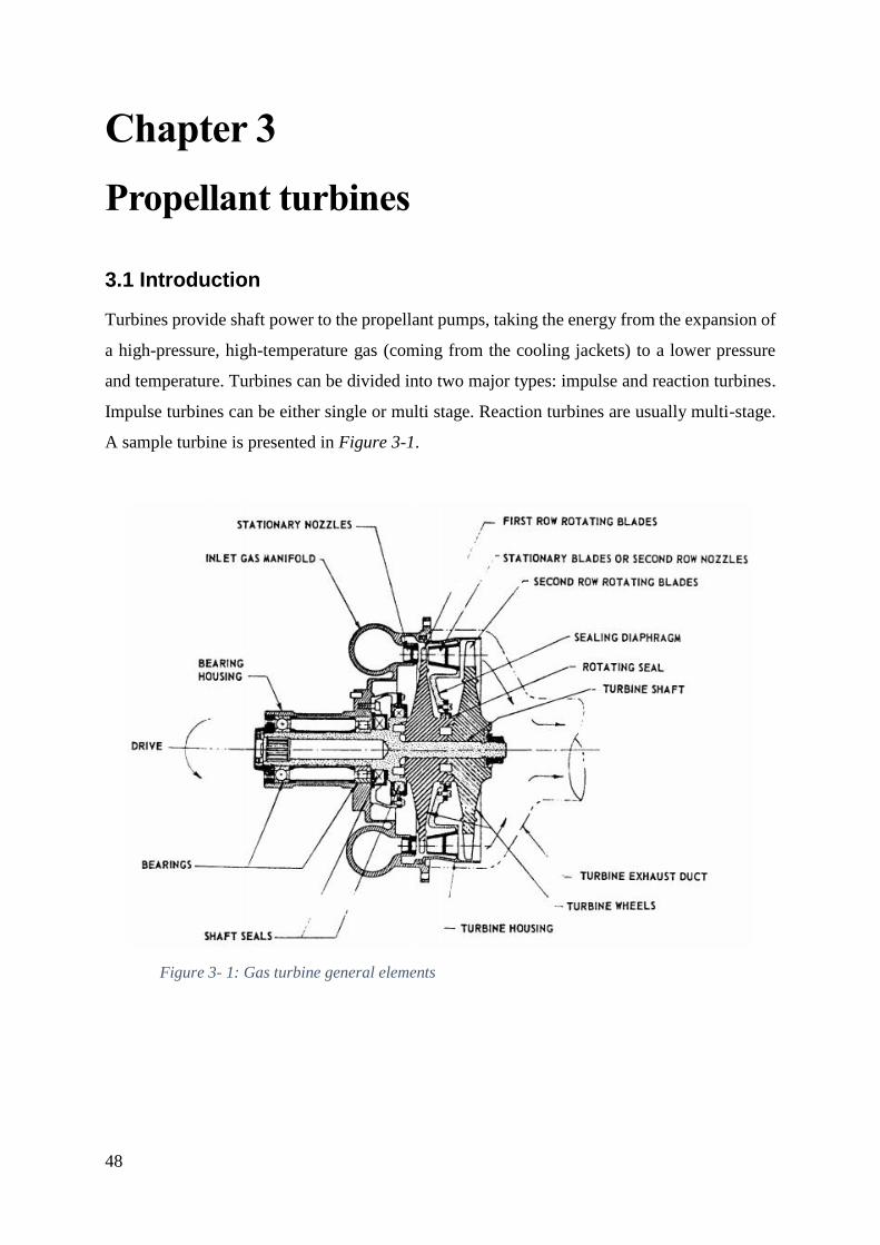
48

Chapter 3

Propellant turbines

3.1 Introduction

Turbines provide shaft power to the propellant pumps, taking the energy from the expansion of

a high-pressure, high-temperature gas (coming from the cooling jackets) to a lower pressure

and temperature. Turbines can be divided into two major types: impulse and reaction turbines.

Impulse turbines can be either single or multi stage. Reaction turbines are usually multi-stage.

A sample turbine is presented in Figure 3-1.

Figure 3- 1: Gas turbine general elements

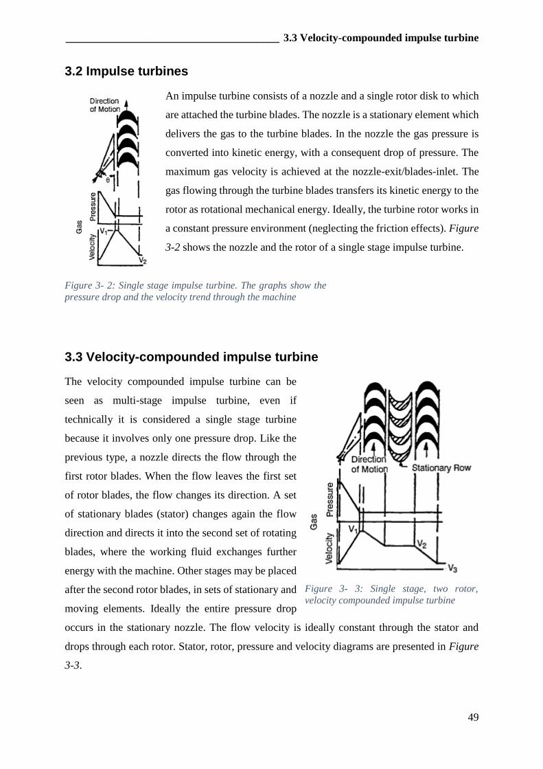
_______________________________________ 3.3 Velocity-compounded impulse turbine

49

3.2 Impulse turbines

An impulse turbine consists of a nozzle and a single rotor disk to which

are attached the turbine blades. The nozzle is a stationary element which

delivers the gas to the turbine blades. In the nozzle the gas pressure is

converted into kinetic energy, with a consequent drop of pressure. The

maximum gas velocity is achieved at the nozzle-exit/blades-inlet. The

gas flowing through the turbine blades transfers its kinetic energy to the

rotor as rotational mechanical energy. Ideally, the turbine rotor works in

a constant pressure environment (neglecting the friction effects). Figure

3-2 shows the nozzle and the rotor of a single stage impulse turbine.

3.3 Velocity-compounded impulse turbine

The velocity compounded impulse turbine can be

seen as multi-stage impulse turbine, even if

technically it is considered a single stage turbine

because it involves only one pressure drop. Like the

previous type, a nozzle directs the flow through the

first rotor blades. When the flow leaves the first set

of rotor blades, the flow changes its direction. A set

of stationary blades (stator) changes again the flow

direction and directs it into the second set of rotating

blades, where the working fluid exchanges further

energy with the machine. Other stages may be placed

after the second rotor blades, in sets of stationary and

moving elements. Ideally the entire pressure drop

occurs in the stationary nozzle. The flow velocity is ideally constant through the stator and

drops through each rotor. Stator, rotor, pressure and velocity diagrams are presented in Figure

3-3.

Figure 3- 2: Single stage impulse turbine. The graphs show the

pressure drop and the velocity trend through the machine

Figure 3- 3: Single stage, two rotor,

velocity compounded impulse turbine

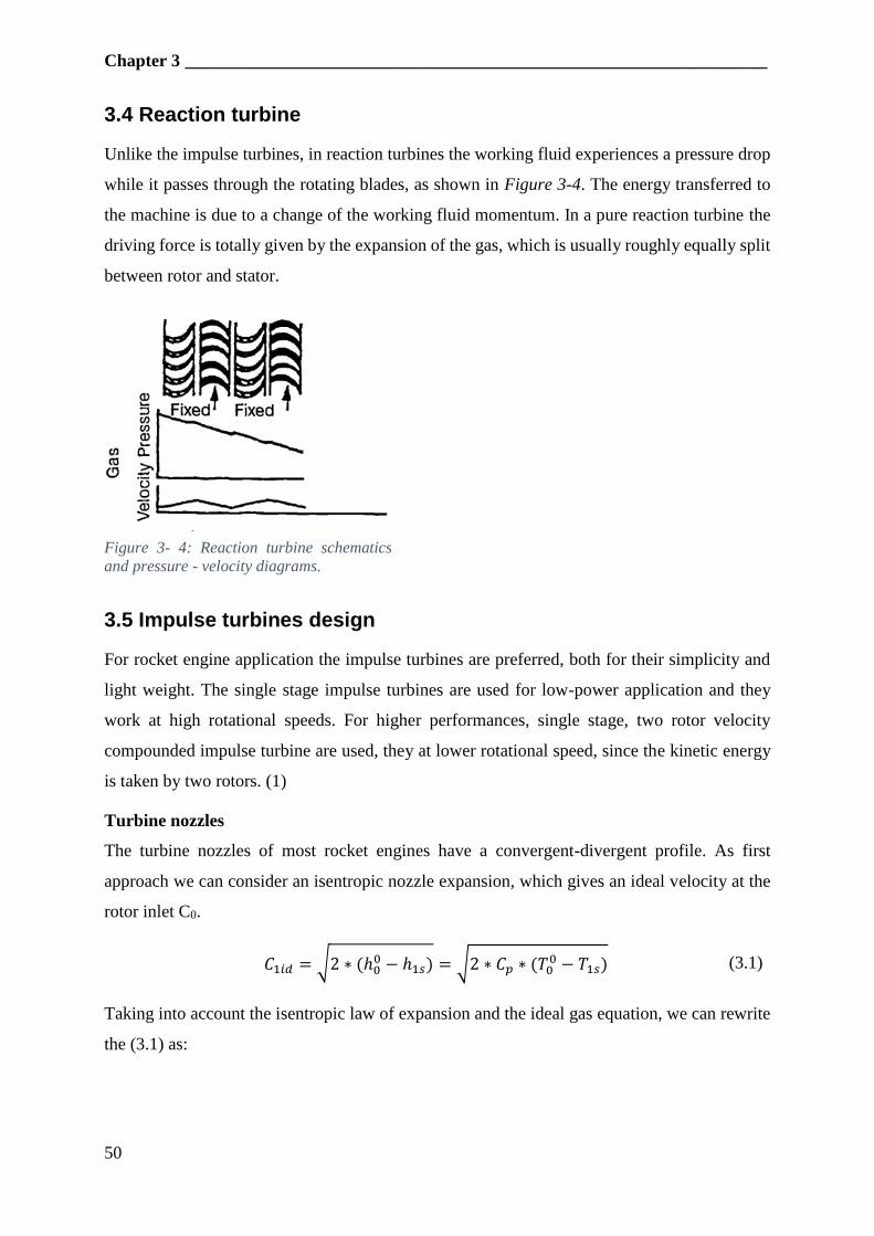
Chapter 3 __________________________________________________________________

50

3.4 Reaction turbine

Unlike the impulse turbines, in reaction turbines the working fluid experiences a pressure drop

while it passes through the rotating blades, as shown in Figure 3-4. The energy transferred to

the machine is due to a change of the working fluid momentum. In a pure reaction turbine the

driving force is totally given by the expansion of the gas, which is usually roughly equally split

between rotor and stator.

3.5 Impulse turbines design

For rocket engine application the impulse turbines are preferred, both for their simplicity and

light weight. The single stage impulse turbines are used for low-power application and they

work at high rotational speeds. For higher performances, single stage, two rotor velocity

compounded impulse turbine are used, they at lower rotational speed, since the kinetic energy

is taken by two rotors. (1)

Turbine nozzles

The turbine nozzles of most rocket engines have a convergent-divergent profile. As first

approach we can consider an isentropic nozzle expansion, which gives an ideal velocity at the

rotor inlet C0.

𝐶1𝑖𝑑 = √2 ∗ (ℎ00 − ℎ1𝑠) = √2 ∗ 𝐶𝑝 ∗ (𝑇0

0 − 𝑇1𝑠) (3.1)

Taking into account the isentropic law of expansion and the ideal gas equation, we can rewrite

the (3.1) as:

Figure 3- 4: Reaction turbine schematics

and pressure - velocity diagrams.

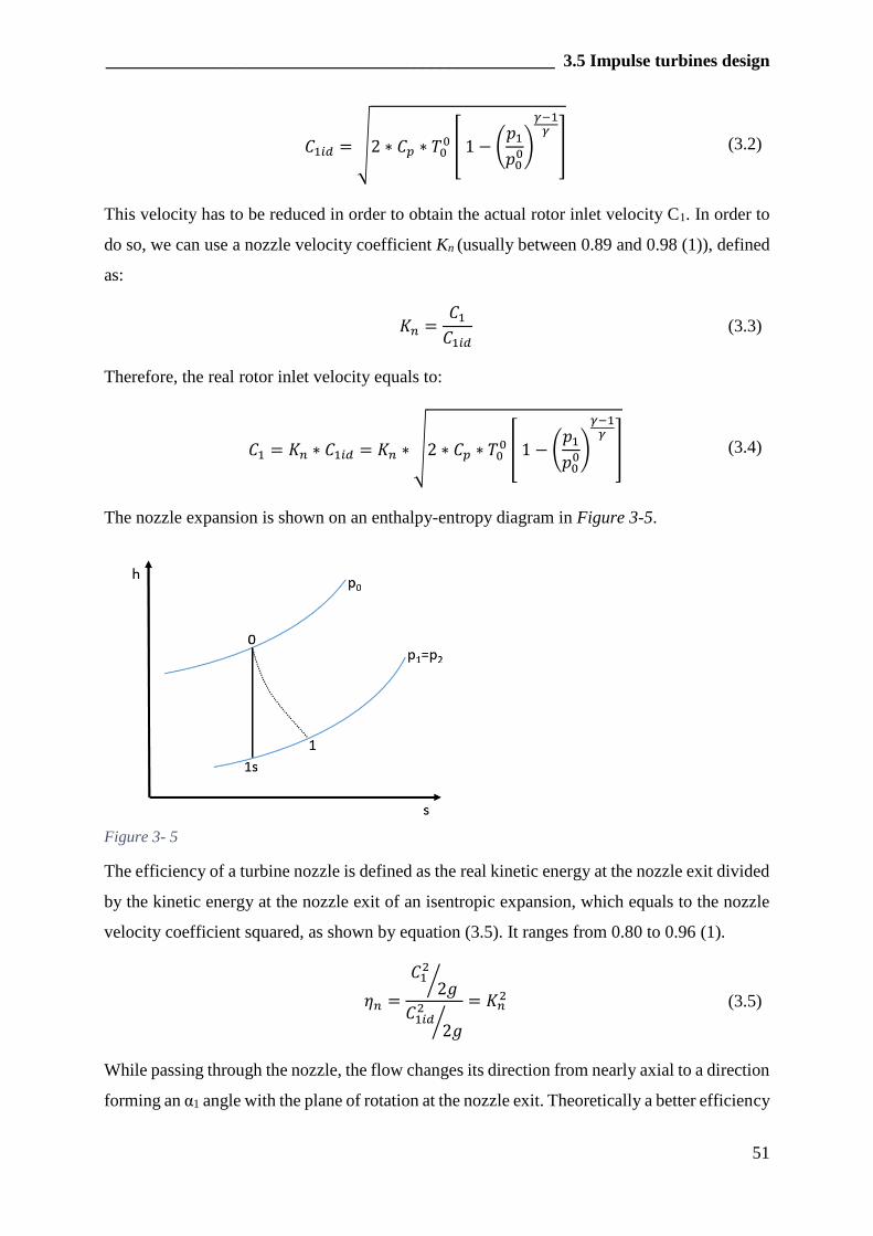
___________________________________________________ 3.5 Impulse turbines design

51

𝐶1𝑖𝑑 = √2 ∗ 𝐶𝑝 ∗ 𝑇00 [ 1 − (

𝑝1

𝑝00)

𝛾−1𝛾

] (3.2)

This velocity has to be reduced in order to obtain the actual rotor inlet velocity C1. In order to

do so, we can use a nozzle velocity coefficient Kn (usually between 0.89 and 0.98 (1)), defined

as:

𝐾𝑛 =𝐶1

𝐶1𝑖𝑑 (3.3)

Therefore, the real rotor inlet velocity equals to:

𝐶1 = 𝐾𝑛 ∗ 𝐶1𝑖𝑑 = 𝐾𝑛 ∗ √2 ∗ 𝐶𝑝 ∗ 𝑇00 [ 1 − (

𝑝1

𝑝00)

𝛾−1𝛾

] (3.4)

The nozzle expansion is shown on an enthalpy-entropy diagram in Figure 3-5.

Figure 3- 5

The efficiency of a turbine nozzle is defined as the real kinetic energy at the nozzle exit divided

by the kinetic energy at the nozzle exit of an isentropic expansion, which equals to the nozzle

velocity coefficient squared, as shown by equation (3.5). It ranges from 0.80 to 0.96 (1).

𝜂𝑛 =

𝐶12

2𝑔⁄

𝐶1𝑖𝑑2

2𝑔⁄

= 𝐾𝑛2 (3.5)

While passing through the nozzle, the flow changes its direction from nearly axial to a direction

forming an α1 angle with the plane of rotation at the nozzle exit. Theoretically a better efficiency

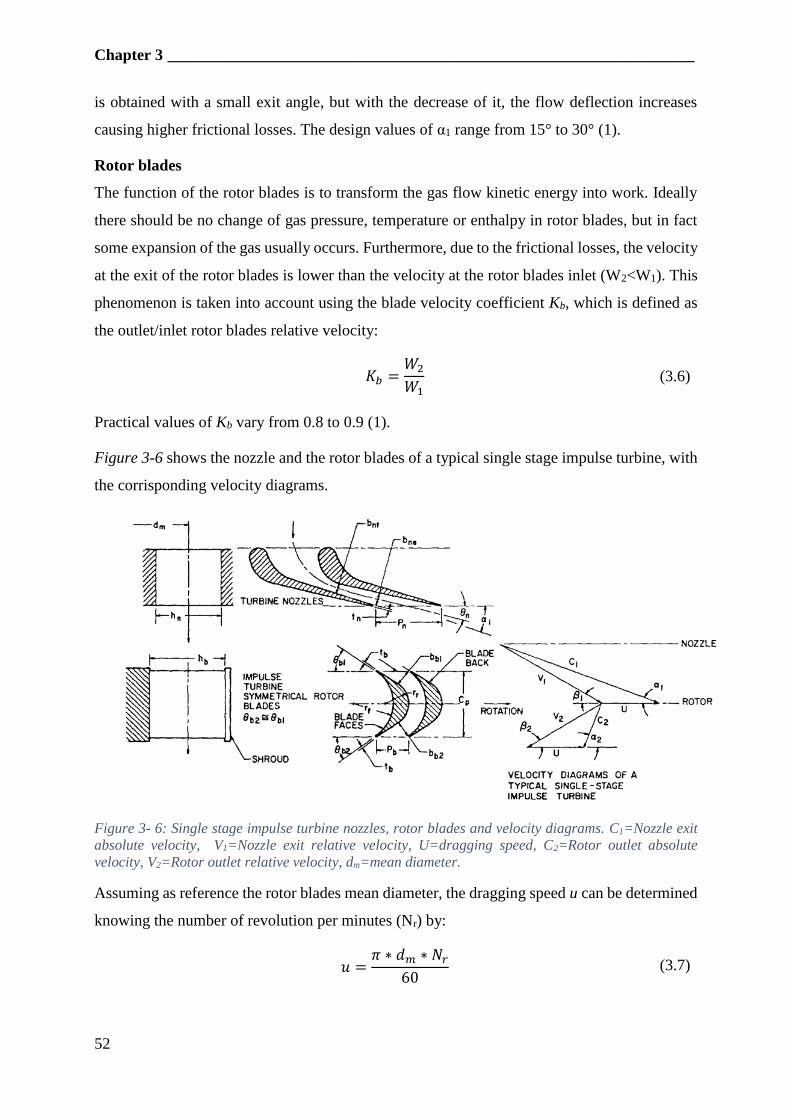
Chapter 3 __________________________________________________________________

52

is obtained with a small exit angle, but with the decrease of it, the flow deflection increases

causing higher frictional losses. The design values of α1 range from 15° to 30° (1).

Rotor blades

The function of the rotor blades is to transform the gas flow kinetic energy into work. Ideally

there should be no change of gas pressure, temperature or enthalpy in rotor blades, but in fact

some expansion of the gas usually occurs. Furthermore, due to the frictional losses, the velocity

at the exit of the rotor blades is lower than the velocity at the rotor blades inlet (W2<W1). This

phenomenon is taken into account using the blade velocity coefficient Kb, which is defined as

the outlet/inlet rotor blades relative velocity:

𝐾𝑏 =𝑊2

𝑊1 (3.6)

Practical values of Kb vary from 0.8 to 0.9 (1).

Figure 3-6 shows the nozzle and the rotor blades of a typical single stage impulse turbine, with

the corrisponding velocity diagrams.

Figure 3- 6: Single stage impulse turbine nozzles, rotor blades and velocity diagrams. C1=Nozzle exit

absolute velocity, V1=Nozzle exit relative velocity, U=dragging speed, C2=Rotor outlet absolute

velocity, V2=Rotor outlet relative velocity, dm=mean diameter.

Assuming as reference the rotor blades mean diameter, the dragging speed u can be determined

knowing the number of revolution per minutes (Nr) by:

𝑢 =𝜋 ∗ 𝑑𝑚 ∗ 𝑁𝑟

60 (3.7)

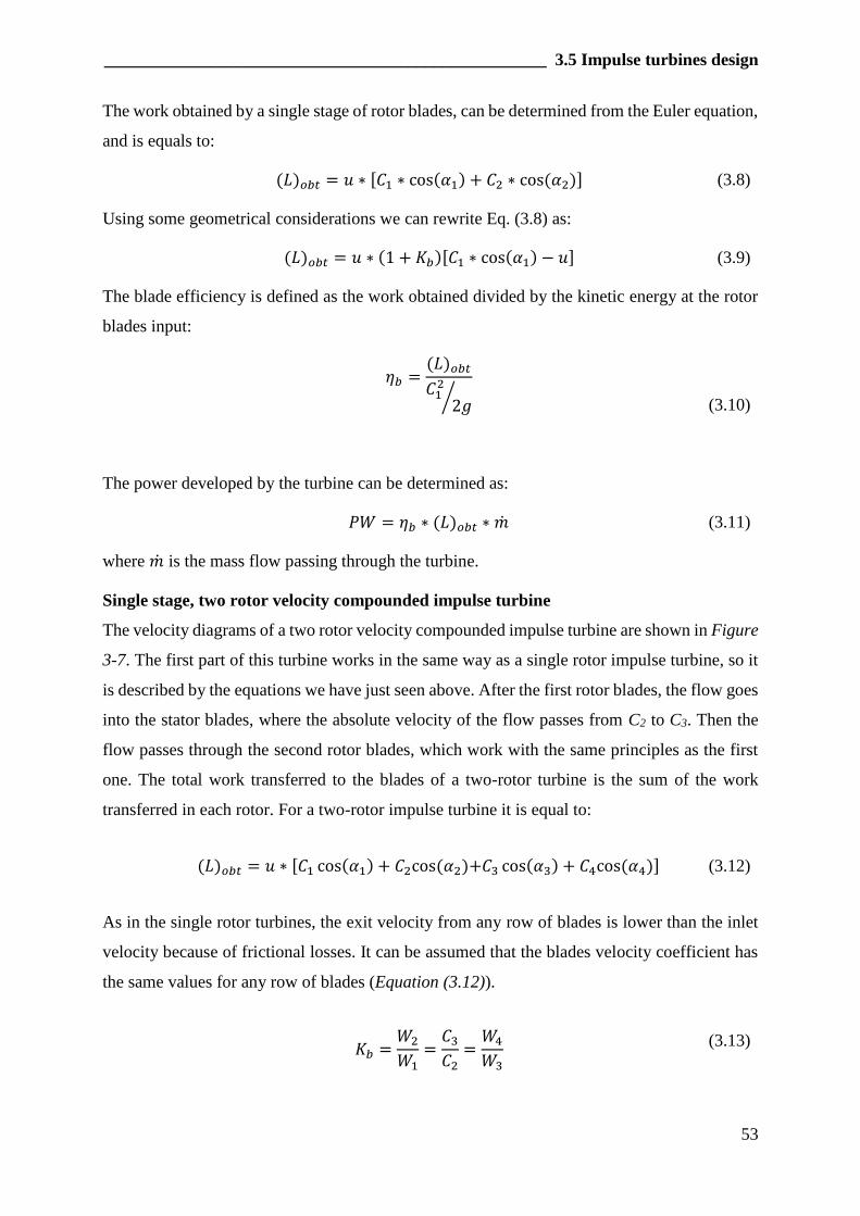
___________________________________________________ 3.5 Impulse turbines design

53

The work obtained by a single stage of rotor blades, can be determined from the Euler equation,

and is equals to:

(𝐿)𝑜𝑏𝑡 = 𝑢 ∗ [𝐶1 ∗ cos(𝛼1) + 𝐶2 ∗ cos (𝛼2)] (3.8)

Using some geometrical considerations we can rewrite Eq. (3.8) as:

(𝐿)𝑜𝑏𝑡 = 𝑢 ∗ (1 + 𝐾𝑏)[𝐶1 ∗ cos(𝛼1) − 𝑢] (3.9)

The blade efficiency is defined as the work obtained divided by the kinetic energy at the rotor

blades input:

𝜂𝑏 =(𝐿)𝑜𝑏𝑡

𝐶12

2𝑔⁄

(3.10)

The power developed by the turbine can be determined as:

𝑃𝑊 = 𝜂𝑏 ∗ (𝐿)𝑜𝑏𝑡 ∗ �� (3.11)

where �� is the mass flow passing through the turbine.

Single stage, two rotor velocity compounded impulse turbine

The velocity diagrams of a two rotor velocity compounded impulse turbine are shown in Figure

3-7. The first part of this turbine works in the same way as a single rotor impulse turbine, so it

is described by the equations we have just seen above. After the first rotor blades, the flow goes

into the stator blades, where the absolute velocity of the flow passes from C2 to C3. Then the

flow passes through the second rotor blades, which work with the same principles as the first

one. The total work transferred to the blades of a two-rotor turbine is the sum of the work

transferred in each rotor. For a two-rotor impulse turbine it is equal to:

(𝐿)𝑜𝑏𝑡 = 𝑢 ∗ [𝐶1 cos(𝛼1) + 𝐶2cos (𝛼2)+𝐶3 cos(𝛼3) + 𝐶4cos (𝛼4)] (3.12)

As in the single rotor turbines, the exit velocity from any row of blades is lower than the inlet

velocity because of frictional losses. It can be assumed that the blades velocity coefficient has

the same values for any row of blades (Equation (3.12)).

𝐾𝑏 =𝑊2

𝑊1=

𝐶3

𝐶2=

𝑊4

𝑊3

(3.13)

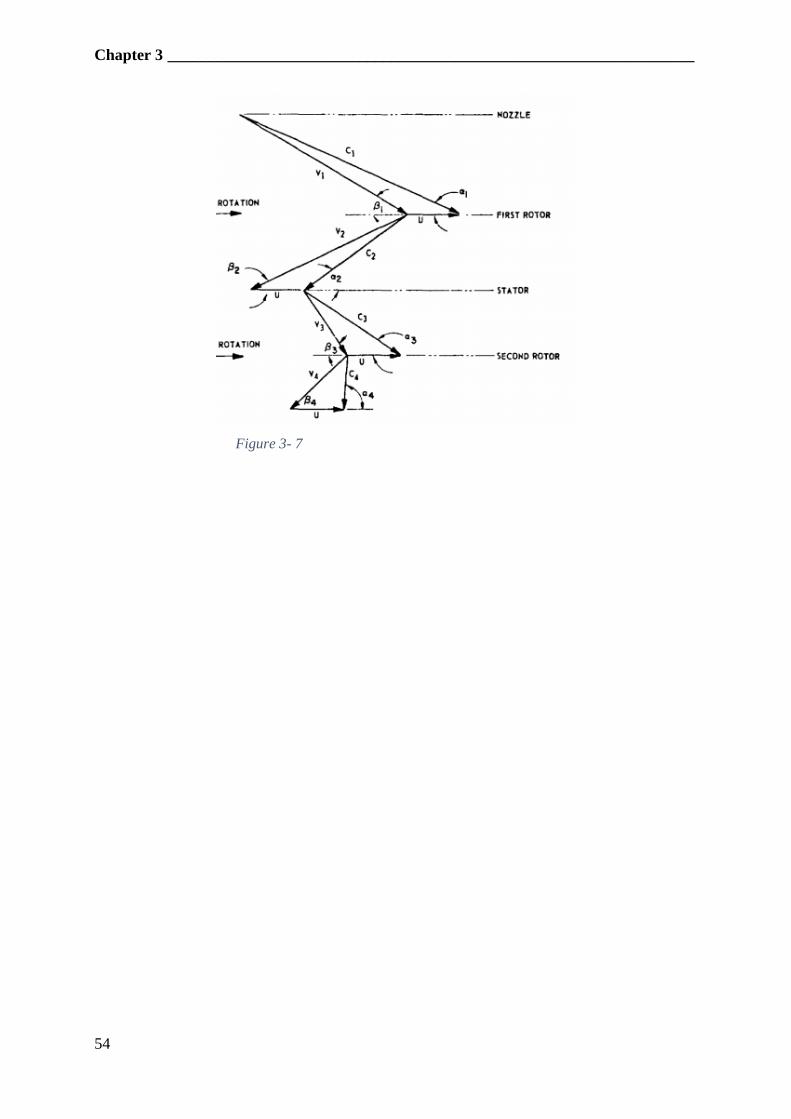
Chapter 3 __________________________________________________________________

54

Figure 3- 7

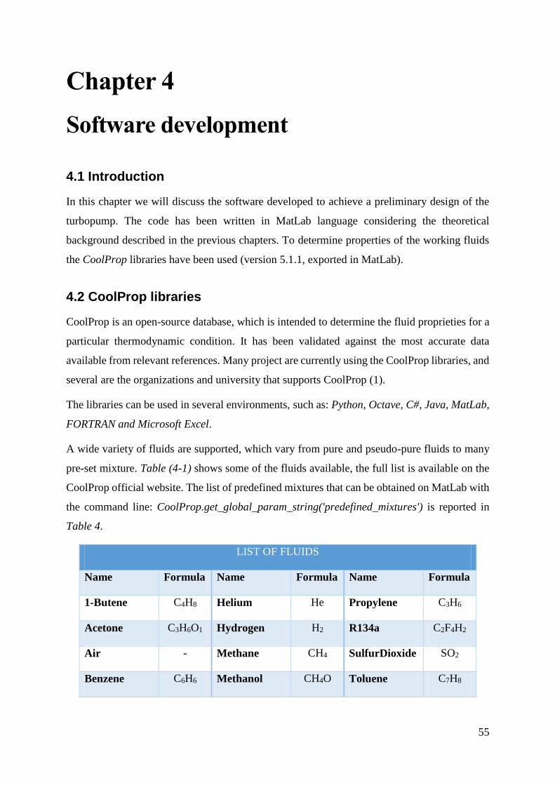
55

Chapter 4

Software development

4.1 Introduction

In this chapter we will discuss the software developed to achieve a preliminary design of the

turbopump. The code has been written in MatLab language considering the theoretical

background described in the previous chapters. To determine properties of the working fluids

the CoolProp libraries have been used (version 5.1.1, exported in MatLab).

4.2 CoolProp libraries

CoolProp is an open-source database, which is intended to determine the fluid proprieties for a

particular thermodynamic condition. It has been validated against the most accurate data

available from relevant references. Many project are currently using the CoolProp libraries, and

several are the organizations and university that supports CoolProp (1).

The libraries can be used in several environments, such as: Python, Octave, C#, Java, MatLab,

FORTRAN and Microsoft Excel.

A wide variety of fluids are supported, which vary from pure and pseudo-pure fluids to many

pre-set mixture. Table (4-1) shows some of the fluids available, the full list is available on the

CoolProp official website. The list of predefined mixtures that can be obtained on MatLab with

the command line: CoolProp.get_global_param_string('predefined_mixtures') is reported in

Table 4.

LIST OF FLUIDS

Name Formula Name Formula Name Formula

1-Butene C4H8 Helium He Propylene C3H6

Acetone C3H6O1 Hydrogen H2 R134a C2F4H2

Air - Methane CH4 SulfurDioxide SO2

Benzene C6H6 Methanol CH4O Toluene C7H8

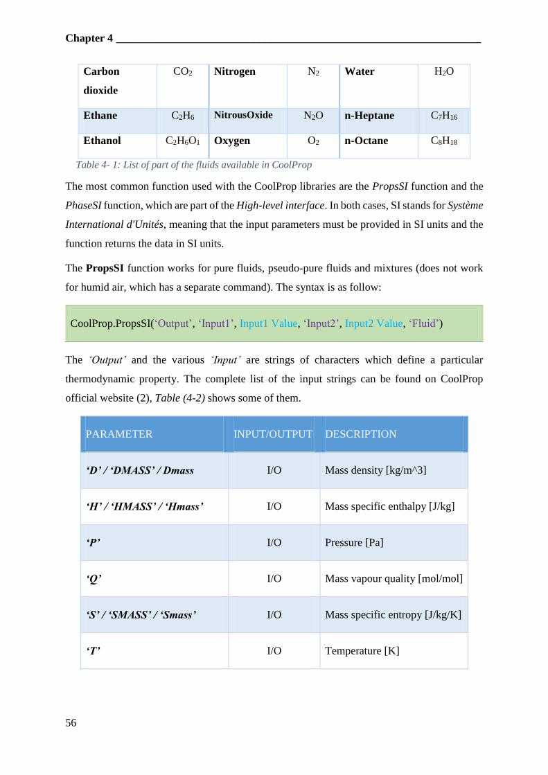
Chapter 4 __________________________________________________________________

56

Carbon

dioxide

CO2 Nitrogen N2 Water H2O

Ethane C2H6 NitrousOxide N2O n-Heptane C7H16

Ethanol C2H6O1 Oxygen O2 n-Octane C8H18

Table 4- 1: List of part of the fluids available in CoolProp

The most common function used with the CoolProp libraries are the PropsSI function and the

PhaseSI function, which are part of the High-level interface. In both cases, SI stands for Système

International d'Unités, meaning that the input parameters must be provided in SI units and the

function returns the data in SI units.

The PropsSI function works for pure fluids, pseudo-pure fluids and mixtures (does not work

for humid air, which has a separate command). The syntax is as follow:

CoolProp.PropsSI(‘Output’, ‘Input1’, Input1 Value, ‘Input2’, Input2 Value, ‘Fluid’)

The ‘Output’ and the various ‘Input’ are strings of characters which define a particular

thermodynamic property. The complete list of the input strings can be found on CoolProp

official website (2), Table (4-2) shows some of them.

PARAMETER INPUT/OUTPUT DESCRIPTION

‘D’ / ‘DMASS’ / Dmass I/O Mass density [kg/m^3]

‘H’ / ‘HMASS’ / ‘Hmass’ I/O Mass specific enthalpy [J/kg]

‘P’ I/O Pressure [Pa]

‘Q’ I/O Mass vapour quality [mol/mol]

‘S’ / ‘SMASS’ / ‘Smass’ I/O Mass specific entropy [J/kg/K]

‘T’ I/O Temperature [K]

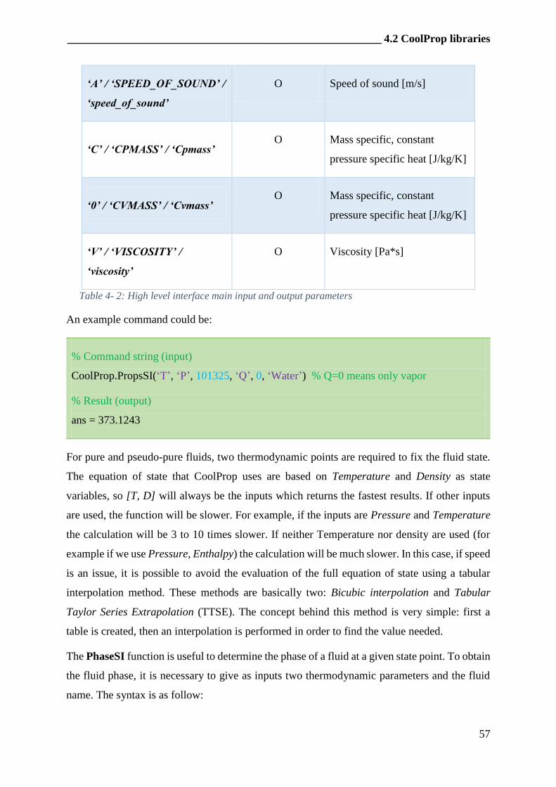
________________________________________________________ 4.2 CoolProp libraries

57

‘A’ / ‘SPEED_OF_SOUND’ /

‘speed_of_sound’

O Speed of sound [m/s]

‘C’ / ‘CPMASS’ / ‘Cpmass’ O Mass specific, constant

pressure specific heat [J/kg/K]

‘0’ / ‘CVMASS’ / ‘Cvmass’ O Mass specific, constant

pressure specific heat [J/kg/K]

‘V’ / ‘VISCOSITY’ /

‘viscosity’

O Viscosity [Pa*s]

Table 4- 2: High level interface main input and output parameters

An example command could be:

% Command string (input)

CoolProp.PropsSI(‘T’, ‘P’, 101325, ‘Q’, 0, ‘Water’) % Q=0 means only vapor

% Result (output)

ans = 373.1243

For pure and pseudo-pure fluids, two thermodynamic points are required to fix the fluid state.

The equation of state that CoolProp uses are based on Temperature and Density as state

variables, so [T, D] will always be the inputs which returns the fastest results. If other inputs

are used, the function will be slower. For example, if the inputs are Pressure and Temperature

the calculation will be 3 to 10 times slower. If neither Temperature nor density are used (for

example if we use Pressure, Enthalpy) the calculation will be much slower. In this case, if speed

is an issue, it is possible to avoid the evaluation of the full equation of state using a tabular

interpolation method. These methods are basically two: Bicubic interpolation and Tabular

Taylor Series Extrapolation (TTSE). The concept behind this method is very simple: first a

table is created, then an interpolation is performed in order to find the value needed.

The PhaseSI function is useful to determine the phase of a fluid at a given state point. To obtain

the fluid phase, it is necessary to give as inputs two thermodynamic parameters and the fluid

name. The syntax is as follow:

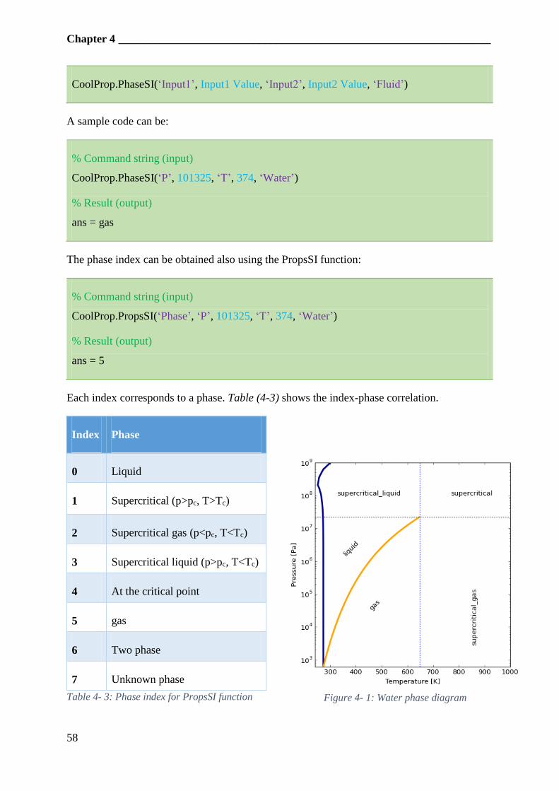
Chapter 4 __________________________________________________________________

58

CoolProp.PhaseSI(‘Input1’, Input1 Value, ‘Input2’, Input2 Value, ‘Fluid’)

A sample code can be:

% Command string (input)

CoolProp.PhaseSI(‘P’, 101325, ‘T’, 374, ‘Water’)

% Result (output)

ans = gas

The phase index can be obtained also using the PropsSI function:

% Command string (input)

CoolProp.PropsSI(‘Phase’, ‘P’, 101325, ‘T’, 374, ‘Water’)

% Result (output)

ans = 5

Each index corresponds to a phase. Table (4-3) shows the index-phase correlation.

Index Phase

0 Liquid

1 Supercritical (p>pc, T>Tc)

2 Supercritical gas (p<pc, T<Tc)

3 Supercritical liquid (p>pc, T<Tc)

4 At the critical point

5 gas

6 Two phase

7 Unknown phase

Table 4- 3: Phase index for PropsSI function Figure 4- 1: Water phase diagram

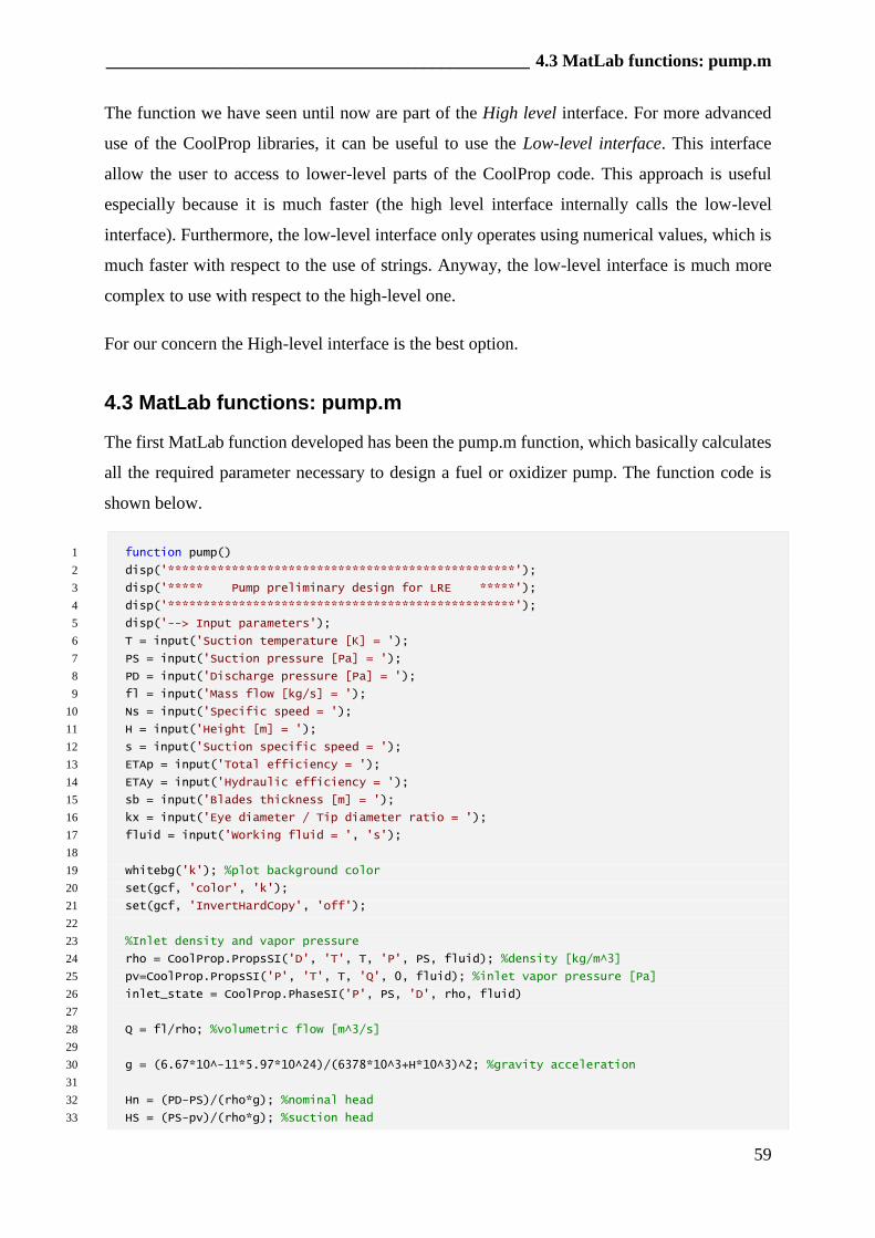
________________________________________________ 4.3 MatLab functions: pump.m

59

The function we have seen until now are part of the High level interface. For more advanced

use of the CoolProp libraries, it can be useful to use the Low-level interface. This interface

allow the user to access to lower-level parts of the CoolProp code. This approach is useful

especially because it is much faster (the high level interface internally calls the low-level

interface). Furthermore, the low-level interface only operates using numerical values, which is

much faster with respect to the use of strings. Anyway, the low-level interface is much more

complex to use with respect to the high-level one.

For our concern the High-level interface is the best option.

4.3 MatLab functions: pump.m

The first MatLab function developed has been the pump.m function, which basically calculates

all the required parameter necessary to design a fuel or oxidizer pump. The function code is

shown below.

function pump() 1

disp('*************************************************'); 2

disp('***** Pump preliminary design for LRE *****'); 3

disp('*************************************************'); 4

disp('--> Input parameters'); 5

T = input('Suction temperature [K] = '); 6

PS = input('Suction pressure [Pa] = '); 7

PD = input('Discharge pressure [Pa] = '); 8

fl = input('Mass flow [kg/s] = '); 9

Ns = input('Specific speed = '); 10

H = input('Height [m] = '); 11

s = input('Suction specific speed = '); 12

ETAp = input('Total efficiency = '); 13

ETAy = input('Hydraulic efficiency = '); 14

sb = input('Blades thickness [m] = '); 15

kx = input('Eye diameter / Tip diameter ratio = '); 16

fluid = input('Working fluid = ', 's'); 17

18

whitebg('k'); %plot background color 19

set(gcf, 'color', 'k'); 20

set(gcf, 'InvertHardCopy', 'off'); 21

22

%Inlet density and vapor pressure 23

rho = CoolProp.PropsSI('D', 'T', T, 'P', PS, fluid); %density [kg/m^3] 24

pv=CoolProp.PropsSI('P', 'T', T, 'Q', 0, fluid); %inlet vapor pressure [Pa] 25

inlet_state = CoolProp.PhaseSI('P', PS, 'D', rho, fluid) 26

27

Q = fl/rho; %volumetric flow [m^3/s] 28

29

g = (6.67*10^-11*5.97*10^24)/(6378*10^3+H*10^3)^2; %gravity acceleration 30

31

Hn = (PD-PS)/(rho*g); %nominal head 32

HS = (PS-pv)/(rho*g); %suction head 33

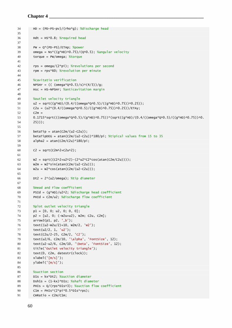
Chapter 4 __________________________________________________________________

60

HD = (PD-PS-pv)/(rho*g); %discharge head 34

35

Hdt = HS*0.8; %required head 36

37

PW = Q*(PD-PS)/ETAp; %power 38

omega = Ns*((g*HD)^0.75)/(Q^0.5); %angular velocity 39

torque = PW/omega; %torque 40

41

rps = omega/(2*pi); %revolutions per second 42

rpm = rps*60; %revolution per minute 43

44

%cavitatio verification 45

NPSHr = (( (omega*Q^0.5)/s)^(4/3))/g; 46

Hsc = HS-NPSHr; %anticavitation margin 47

48

%outlet velocity triangle 49

u2 = sqrt((g*HD)/(0.4/((omega*Q^0.5)/((g*HD)^0.75))^0.25)); 50

C2u = (u2*(0.4/((omega*Q^0.5)/((g*HD)^0.75))^0.25))/ETAy; 51

C2m = 52

0.1715*sqrt(((omega*Q^0.5)/(g*HD)^0.75))*(sqrt((g*HD)/(0.4/((omega*Q^0.5)/((g*HD)^0.75))^0.53

25))); 54

55

betaTip = atan(C2m/(u2-C2u)); 56

betaTipDEG = atan(C2m/(u2-C2u))*180/pi; %tipical values from 15 to 35 57

alpha2 = atan(C2m/C2u)*180/pi; 58

59

C2 = sqrt(C2m^2+C2u^2); 60

61

W2 = sqrt((C2^2+u2^2)-(2*u2*C2*cos(atan(C2m/C2u)))); 62

W2m = W2*sin(atan(C2m/(u2-C2u))); 63

W2u = W2*cos(atan(C2m/(u2-C2u))); 64

65

Dt2 = 2*(u2/omega); %tip diameter 66

67

%Head and Flow coefficient 68

PSId = (g*HD)/u2^2; %discharge head coefficient 69

PHId = C2m/u2; %discharge flow coefficient 70

71

%plot outlet velocity triangle 72

p1 = [0, 0; u2, 0; 0, 0]; 73

p2 = [u2, 0; (-W2u+u2), W2m; C2u, C2m]; 74

arrow3(p1, p2, '_b'); 75

text((u2-W2u/2)+10, W2m/2, 'W2'); 76

text(u2/2, 1, 'u2'); 77

text(C2u/2-25, C2m/2, 'C2'); 78

text(u2/6, C2m/10, '\alpha', 'FontSize', 12); 79

text(u2-u2/6, C2m/10, '\beta', 'FontSize', 12); 80

title('Outlet velocity triangle'); 81

text(0, C2m, datestr(clock)); 82

xlabel('[m/s]'); 83

ylabel('[m/s]'); 84

85

%suction section 86

D1s = kx*Dt2; %suction diameter 87

Dsh1s = (1-kx)*D1s; %shaft diameter 88

PHIs = Q/(rps*D1s^3); %suction flow coefficient 89

C1m = PHIs*(2*pi*0.5*D1s*rps); 90

CmRatio = C2m/C1m; 91

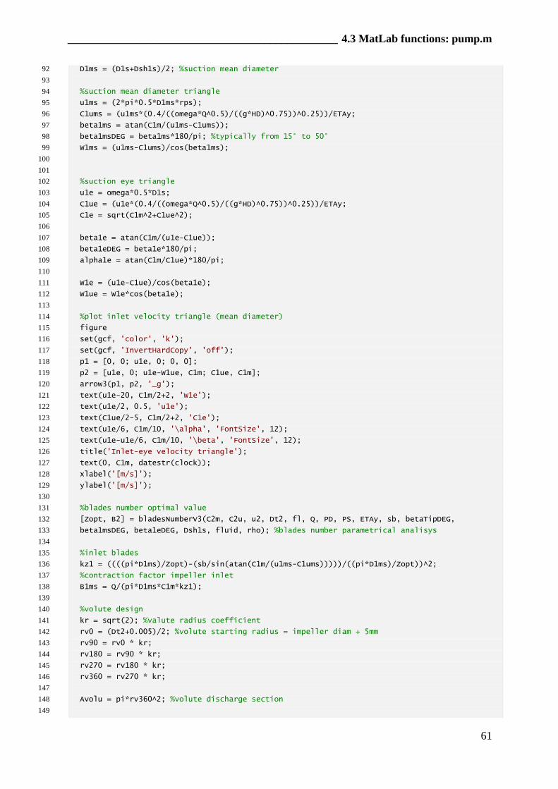
________________________________________________ 4.3 MatLab functions: pump.m

61

D1ms = (D1s+Dsh1s)/2; %suction mean diameter 92

93

%suction mean diameter triangle 94

u1ms = (2*pi*0.5*D1ms*rps); 95

C1ums = (u1ms*(0.4/((omega*Q^0.5)/((g*HD)^0.75))^0.25))/ETAy; 96

beta1ms = atan(C1m/(u1ms-C1ums)); 97

beta1msDEG = beta1ms*180/pi; %typically from 15° to 50° 98

W1ms = (u1ms-C1ums)/cos(beta1ms); 99

100

101

%suction eye triangle 102

u1e = omega*0.5*D1s; 103

C1ue = (u1e*(0.4/((omega*Q^0.5)/((g*HD)^0.75))^0.25))/ETAy; 104

C1e = sqrt(C1m^2+C1ue^2); 105

106

beta1e = atan(C1m/(u1e-C1ue)); 107

beta1eDEG = beta1e*180/pi; 108

alpha1e = atan(C1m/C1ue)*180/pi; 109

110

W1e = (u1e-C1ue)/cos(beta1e); 111

W1ue = W1e*cos(beta1e); 112

113

%plot inlet velocity triangle (mean diameter) 114

figure 115

set(gcf, 'color', 'k'); 116

set(gcf, 'InvertHardCopy', 'off'); 117

p1 = [0, 0; u1e, 0; 0, 0]; 118

p2 = [u1e, 0; u1e-W1ue, C1m; C1ue, C1m]; 119

arrow3(p1, p2, '_g'); 120

text(u1e-20, C1m/2+2, 'W1e'); 121

text(u1e/2, 0.5, 'u1e'); 122

text(C1ue/2-5, C1m/2+2, 'C1e'); 123

text(u1e/6, C1m/10, '\alpha', 'FontSize', 12); 124

text(u1e-u1e/6, C1m/10, '\beta', 'FontSize', 12); 125

title('Inlet-eye velocity triangle'); 126

text(0, C1m, datestr(clock)); 127

xlabel('[m/s]'); 128

ylabel('[m/s]'); 129

130

%blades number optimal value 131

[Zopt, B2] = bladesNumberV3(C2m, C2u, u2, Dt2, fl, Q, PD, PS, ETAy, sb, betaTipDEG, 132

beta1msDEG, beta1eDEG, Dsh1s, fluid, rho); %blades number parametrical analisys 133

134

%inlet blades 135

kz1 = ((((pi*D1ms)/Zopt)-(sb/sin(atan(C1m/(u1ms-C1ums)))))/((pi*D1ms)/Zopt))^2; 136

%contraction factor impeller inlet 137

B1ms = Q/(pi*D1ms*C1m*kz1); 138

139

%volute design 140

kr = sqrt(2); %valute radius coefficient 141

rv0 = (Dt2+0.005)/2; %volute starting radius = impeller diam + 5mm 142

rv90 = rv0 * kr; 143

rv180 = rv90 * kr; 144

rv270 = rv180 * kr; 145

rv360 = rv270 * kr; 146

147

Avolu = pi*rv360^2; %volute discharge section 148

149

Chapter 4 __________________________________________________________________

62

Cvolu = Q/Avolu; %Volute discharge velocity 150

151

Pvolut = (0.5*rho*C2m^2+PD)-0.5*rho*Cvolu^2; %Volute discharge pressure 152

153

DeltaPvolut = Pvolut - PD; %Volute pressure increment 154

155

%material strength 156

stress = rho * u2^2 /(1E6) %[MPa] 157

158

%save data to file 159

fileID = fopen('Pump propeties.txt', 'w'); 160

161

fprintf(fileID, '%-40s\r\n', datestr(clock)); 162

163

fprintf(fileID, '************************************************************\r\n'); 164

fprintf(fileID, '************************************************************\r\n'); 165

fprintf(fileID, '******** ********\r\n'); 166

fprintf(fileID, '******** Pump properties ********\r\n'); 167

fprintf(fileID, '******** ********\r\n'); 168

fprintf(fileID, '************************************************************\r\n'); 169

fprintf(fileID, '************************************************************\r\n\r\n'); 170

fprintf(fileID, '----------------------Input Parameters----------------------\r\n'); 171

fprintf(fileID, '%-40s %12s\r\n', 'Fluid = ', fluid); 172

fprintf(fileID, '%-40s %12.4f\r\n', 'Suction temperature T [K] = ', T); 173

fprintf(fileID, '%-40s %12.4f\r\n', 'Scution Pressure PS [Pa] = ', PS); 174

fprintf(fileID, '%-40s %12.4f\r\n', 'Mass flow fl [kg/s] = ', fl); 175

fprintf(fileID, '%-40s %12.4f\r\n', 'Discharge pressure PD [Pa] = ', PD); 176

fprintf(fileID, '%-40s %12.4f\r\n', 'Specific speed Ns = ', Ns); 177

fprintf(fileID, '%-40s %12.4f\r\n', 'Suction speed s = ', s); 178

fprintf(fileID, '%-40s %12.4f\r\n', 'Height H [m] = ', H); 179

fprintf(fileID, '%-40s %12.4f\r\n', 'Efficiency ETAp = ', ETAp); 180

fprintf(fileID, '%-40s %12.4f\r\n', 'Hydraulic efficiency ETAy = ', ETAy); 181

fprintf(fileID, '\r\n\r\n-------------------------- Results -------------------------182

\r\n'); 183

fprintf(fileID, '%-40s %12.4f\r\n', 'Density rho [kg/m^3] = ', rho); 184

fprintf(fileID, '%-40s %12.4f\r\n', 'Vapor pressure pv [Pa] = ', pv); 185

fprintf(fileID, '%-40s %12.4f\r\n', 'Volumetric flow Q [m^3/s] = ', Q); 186

fprintf(fileID, '%-40s %12.4f\r\n', 'Gravity acceleration g [m/s^2] = ', g); 187

fprintf(fileID, '%-40s %12.4f\r\n', 'Nominal Head Hn [m] = ', Hn); 188

fprintf(fileID, '%-40s %12.4f\r\n', 'Suction head HS [m] = ', HS); 189

fprintf(fileID, '%-40s %12.4f\r\n', 'Dischagre head HD [m] = ', HD); 190

fprintf(fileID, '%-40s %12.4f\r\n', 'Minimum required head Hdt [m] = ', Hdt); 191

fprintf(fileID, '%-40s %12.4f\r\n', 'Power PW [W] = ', PW); 192

fprintf(fileID, '%-40s %12.4f\r\n', 'Angular velocity omega [rad/s] = ', omega); 193

fprintf(fileID, '%-40s %12.4f\r\n', 'torque [N/m] = ', torque); 194

fprintf(fileID, '%-40s %12.4f\r\n', 'Revolution per second rps [1/s] = ', rps); 195

fprintf(fileID, '%-40s %12.4f\r\n', 'Revolution per minute rpm [1/min] = ', rpm); 196

fprintf(fileID, '%-40s %12.4f\r\n', 'NPSHr [m] = ', NPSHr); 197

fprintf(fileID, '%-40s %12.4f\r\n', 'Anticavitation margin Hsc [m] = ', Hsc); 198

fprintf(fileID, '%-40s %12.4f\r\n', 'Absolute velocity (outlet) C2 [m/s] = ', C2); 199

fprintf(fileID, '%-40s %12.4f\r\n', 'Dragging speed (outlet) u2 [m/s] = ', u2); 200

fprintf(fileID, '%-40s %12.4f\r\n', 'Relative velocty (outlet) W2 [m/s] = ', W2); 201

fprintf(fileID, '%-40s %12.4f', 'Beta angle impeller tip betaTip [deg] = ', betaTipDEG); 202

if betaTipDEG >= 15 && betaTipDEG <= 35 203

fprintf(fileID, ' *OK*\r\n'); 204

else 205

fprintf(fileID, ' *****ERROR*****\r\n'); 206

end 207

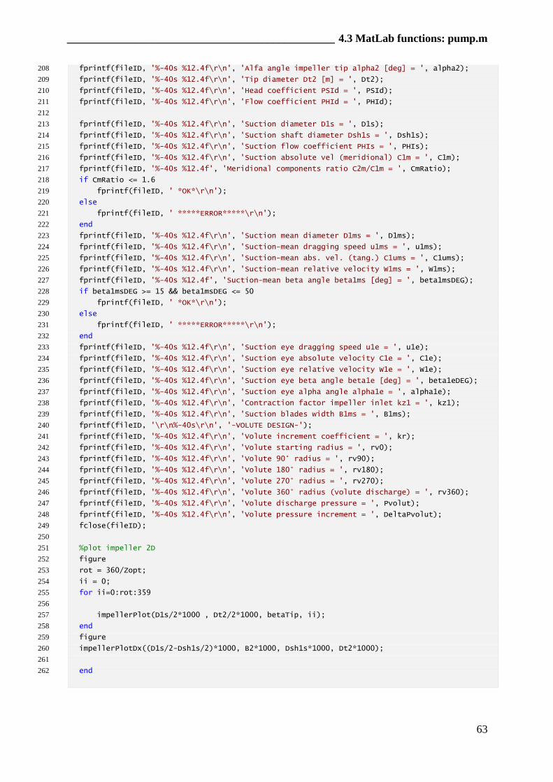
________________________________________________ 4.3 MatLab functions: pump.m

63

fprintf(fileID, '%-40s %12.4f\r\n', 'Alfa angle impeller tip alpha2 [deg] = ', alpha2); 208

fprintf(fileID, '%-40s %12.4f\r\n', 'Tip diameter Dt2 [m] = ', Dt2); 209

fprintf(fileID, '%-40s %12.4f\r\n', 'Head coefficient PSId = ', PSId); 210

fprintf(fileID, '%-40s %12.4f\r\n', 'Flow coefficient PHId = ', PHId); 211

212

fprintf(fileID, '%-40s %12.4f\r\n', 'Suction diameter D1s = ', D1s); 213

fprintf(fileID, '%-40s %12.4f\r\n', 'Suction shaft diameter Dsh1s = ', Dsh1s); 214

fprintf(fileID, '%-40s %12.4f\r\n', 'Suction flow coefficient PHIs = ', PHIs); 215

fprintf(fileID, '%-40s %12.4f\r\n', 'Suction absolute vel (meridional) C1m = ', C1m); 216

fprintf(fileID, '%-40s %12.4f', 'Meridional components ratio C2m/C1m = ', CmRatio); 217

if CmRatio <= 1.6 218

fprintf(fileID, ' *OK*\r\n'); 219

else 220

fprintf(fileID, ' *****ERROR*****\r\n'); 221

end 222

fprintf(fileID, '%-40s %12.4f\r\n', 'Suction mean diameter D1ms = ', D1ms); 223

fprintf(fileID, '%-40s %12.4f\r\n', 'Suction-mean dragging speed u1ms = ', u1ms); 224

fprintf(fileID, '%-40s %12.4f\r\n', 'Suction-mean abs. vel. (tang.) C1ums = ', C1ums); 225

fprintf(fileID, '%-40s %12.4f\r\n', 'Suction-mean relative velocity W1ms = ', W1ms); 226

fprintf(fileID, '%-40s %12.4f', 'Suction-mean beta angle beta1ms [deg] = ', beta1msDEG); 227

if beta1msDEG >= 15 && beta1msDEG <= 50 228

fprintf(fileID, ' *OK*\r\n'); 229

else 230

fprintf(fileID, ' *****ERROR*****\r\n'); 231

end 232

fprintf(fileID, '%-40s %12.4f\r\n', 'Suction eye dragging speed u1e = ', u1e); 233

fprintf(fileID, '%-40s %12.4f\r\n', 'Suction eye absolute velocity C1e = ', C1e); 234

fprintf(fileID, '%-40s %12.4f\r\n', 'Suction eye relative velocity W1e = ', W1e); 235

fprintf(fileID, '%-40s %12.4f\r\n', 'Suction eye beta angle beta1e [deg] = ', beta1eDEG); 236

fprintf(fileID, '%-40s %12.4f\r\n', 'Suction eye alpha angle alpha1e = ', alpha1e); 237

fprintf(fileID, '%-40s %12.4f\r\n', 'Contraction factor impeller inlet kz1 = ', kz1); 238

fprintf(fileID, '%-40s %12.4f\r\n', 'Suction blades width B1ms = ', B1ms); 239

fprintf(fileID, '\r\n%-40s\r\n', '-VOLUTE DESIGN-'); 240

fprintf(fileID, '%-40s %12.4f\r\n', 'Volute increment coefficient = ', kr); 241

fprintf(fileID, '%-40s %12.4f\r\n', 'Volute starting radius = ', rv0); 242

fprintf(fileID, '%-40s %12.4f\r\n', 'Volute 90° radius = ', rv90); 243

fprintf(fileID, '%-40s %12.4f\r\n', 'Volute 180° radius = ', rv180); 244

fprintf(fileID, '%-40s %12.4f\r\n', 'Volute 270° radius = ', rv270); 245

fprintf(fileID, '%-40s %12.4f\r\n', 'Volute 360° radius (volute discharge) = ', rv360); 246

fprintf(fileID, '%-40s %12.4f\r\n', 'Volute discharge pressure = ', Pvolut); 247

fprintf(fileID, '%-40s %12.4f\r\n', 'Volute pressure increment = ', DeltaPvolut); 248

fclose(fileID); 249

250

%plot impeller 2D 251

figure 252

rot = 360/Zopt; 253

ii = 0; 254

for ii=0:rot:359 255

256

impellerPlot(D1s/2*1000 , Dt2/2*1000, betaTip, ii); 257

end 258

figure 259

impellerPlotDx((D1s/2-Dsh1s/2)*1000, B2*1000, Dsh1s*1000, Dt2*1000); 260

261

end 262

Chapter 4 __________________________________________________________________

64

The first part of the code, from line 6 to line 17, asks the input parameters necessary to run the

function. These are: suction temperature, suction pressure, discharge pressure, mass flow,

specific speed, height, suction specific speed, total efficiency, hydraulic efficiency, blades

thickness, eye diameter / tip diameter ratio and the working fluid. After that, the program starts

to calculate the necessary data. The inlet density and the inlet vapor pressure (line 23 to 25) are

determined by the use of the CoolProp libraries. Also a first check about cavitation is performed

through the CoolProp PhaseSI function (line 26) that returns a console feedback about the inlet

fluid state, which can be one of those list in table 4.3.

Once the density is known, it is possible to determine the volumetric flow rate (line 28) using

equation (2.2). The successive line calculates the gravity acceleration as a function of the input

height.

The nominal head, suction head and discharge head are calculated using equation (2.6), while

the required head Hdt, as a first guess, is determined to be the 80% of the suction head (line

36). This value of the required head gives us a first idea of the anti-cavitation margin that should

be obtained.

The power needed by the pump (line 38) is calculated using equation (2.56), the angular

velocity using equation (2.14). It is now possible to determine the required torque dividing the

power by the angular velocity (line 40). Other necessary data are the revolutions per second and

the revolutions per minutes, which are directly related to the angular velocity (line 42 and 43).

The required NPSH results by rearranging equation (2.13). We can now determine the anti-

cavitation margin Hsc (line 47). This values should be compare with the Hdt determined in line

36, which is an esteem of the anti-cavitation margin based on known data.

The next step is to determine the velocity triangles. In all the variables related to the velocity

triangles the subscript “2” stands for the outlet section, while “u” stands for tangential

component and “m” for meridian component. The outlet velocity triangle is determined first.

The starting point is the dragging speed u2 (line 50), which can be calculated using equation

(2.27). It is now possible to determine the tangential component of the absolute velocity using

equation (2.35) and its meridian component by equation (2.36). Being known the two

components of the absolute velocity, it is possible to determine the absolute velocity magnitude

(line 60). In addition we can determine the alpha and beta angles of the velocity triangle by

simple geometrical considerations, that results in equations (2.38) and (2.40). The only

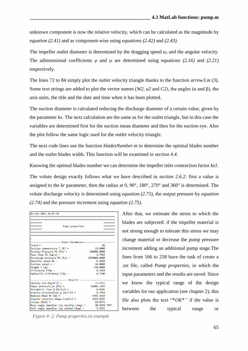
________________________________________________ 4.3 MatLab functions: pump.m

65

unknown component is now the relative velocity, which can be calculated as the magnitude by

equation (2.41) and as component-wise using equations (2.42) and (2.43).

The impeller outlet diameter is determined by the dragging speed u2 and the angular velocity.

The adimensional coefficients φ and ψ are determined using equations (2.16) and (2.21)

respectively.

The lines 72 to 84 simply plot the outlet velocity triangle thanks to the function arrow3.m (3).

Some text strings are added to plot the vector names (W2, u2 and C2), the angles (α and β), the

axis units, the title and the date and time when it has been plotted.

The suction diameter is calculated reducing the discharge diameter of a certain value, given by

the parameter kx. The next calculation are the same as for the outlet triangle, but in this case the

variables are determined first for the suction mean diameter and then for the suction eye. Also

the plot follow the same logic used for the outlet velocity triangle.

The next code lines use the function bladesNumber.m to determine the optimal blades number

and the outlet blades width. This function will be examined in section 4.4.

Knowing the optimal blades number we can determine the impeller inlet contraction factor kz1.

The volute design exactly follows what we have described in section 2.6.2: first a value is

assigned to the kr parameter, then the radius at 0, 90°, 180°, 270° and 360° is determined. The

volute discharge velocity is determined using equation (2.73), the output pressure by equation

(2.74) and the pressure increment using equation (2.75).

After that, we estimate the stress to which the

blades are subjected: if the impeller material is

not strong enough to tolerate this stress we may

change material or decrease the pump pressure

increment adding an additional pump stage.The

lines from 166 to 258 have the task of create a

.txt file, called Pump properties, in which the

input parameters and the results are saved. Since

we know the typical range of the design

variables for our application (see chapter 2), this

file also plots the text “*OK*” if the value is

between the typical range or

Figure 4- 2: Pump properties.txt example

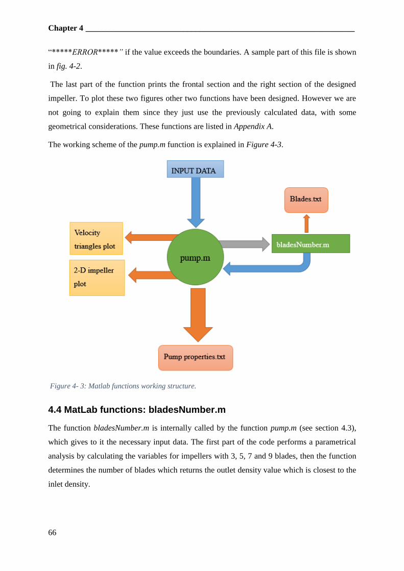
Chapter 4 __________________________________________________________________

66

“*****ERROR*****” if the value exceeds the boundaries. A sample part of this file is shown

in fig. 4-2.

The last part of the function prints the frontal section and the right section of the designed

impeller. To plot these two figures other two functions have been designed. However we are

not going to explain them since they just use the previously calculated data, with some

geometrical considerations. These functions are listed in Appendix A.

The working scheme of the pump.m function is explained in Figure 4-3.

4.4 MatLab functions: bladesNumber.m

The function bladesNumber.m is internally called by the function pump.m (see section 4.3),

which gives to it the necessary input data. The first part of the code performs a parametrical

analysis by calculating the variables for impellers with 3, 5, 7 and 9 blades, then the function

determines the number of blades which returns the outlet density value which is closest to the

inlet density.

Figure 4- 3: Matlab functions working structure.

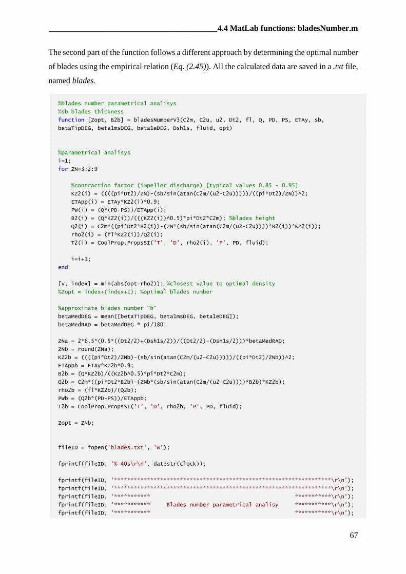
_________________________________________ 4.4 MatLab functions: bladesNumber.m

67

The second part of the function follows a different approach by determining the optimal number

of blades using the empirical relation (Eq. (2.45)). All the calculated data are saved in a .txt file,

named blades.

%blades number parametrical analisys

%sb blades thickness

function [Zopt, B2b] = bladesNumberV3(C2m, C2u, u2, Dt2, fl, Q, PD, PS, ETAy, sb,

betaTipDEG, beta1msDEG, beta1eDEG, Dsh1s, fluid, opt)

%parametrical analisys

i=1;

for ZN=3:2:9

%contraction factor (impeller discharge) [typical values 0.85 - 0.95]

KZ2(i) = ((((pi*Dt2)/ZN)-(sb/sin(atan(C2m/(u2-C2u)))))/((pi*Dt2)/ZN))^2;

ETApp(i) = ETAy*KZ2(i)*0.9;

PW(i) = (Q*(PD-PS))/ETApp(i);

B2(i) = (Q*KZ2(i))/(((KZ2(i))^0.5)*pi*Dt2*C2m); %blades height

Q2(i) = C2m*((pi*Dt2*B2(i))-(ZN*(sb/sin(atan(C2m/(u2-C2u))))*B2(i))*KZ2(i));

rho2(i) = (fl*KZ2(i))/Q2(i);

T2(i) = CoolProp.PropsSI('T', 'D', rho2(i), 'P', PD, fluid);

i=i+1;

end

[v, index] = min(abs(opt-rho2)); %closest value to optimal density

%Zopt = index+(index+1); %optimal blades number

%approximate blades number "b"

betaMedDEG = mean([betaTipDEG, beta1msDEG, beta1eDEG]);

betaMedRAD = betaMedDEG * pi/180;

ZNa = 2*6.5*(0.5*((Dt2/2)+(Dsh1s/2))/((Dt2/2)-(Dsh1s/2)))*betaMedRAD;

ZNb = round(ZNa);

KZ2b = ((((pi*Dt2)/ZNb)-(sb/sin(atan(C2m/(u2-C2u)))))/((pi*Dt2)/ZNb))^2;

ETAppb = ETAy*KZ2b*0.9;

B2b = (Q*KZ2b)/((KZ2b^0.5)*pi*Dt2*C2m);

Q2b = C2m*((pi*Dt2*B2b)-(ZNb*(sb/sin(atan(C2m/(u2-C2u))))*B2b)*KZ2b);

rho2b = (fl*KZ2b)/(Q2b);

PWb = (Q2b*(PD-PS))/ETAppb;

T2b = CoolProp.PropsSI('T', 'D', rho2b, 'P', PD, fluid);

Zopt = ZNb;

fileID = fopen('blades.txt', 'w');

fprintf(fileID, '%-40s\r\n', datestr(clock));

fprintf(fileID, '******************************************************************\r\n');

fprintf(fileID, '******************************************************************\r\n');

fprintf(fileID, '*********** ***********\r\n');

fprintf(fileID, '*********** Blades number parametrical analisy ***********\r\n');

fprintf(fileID, '*********** ***********\r\n');

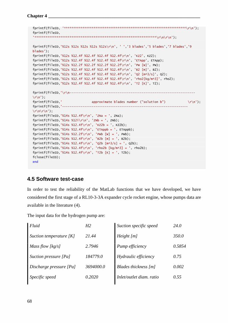
Chapter 4 __________________________________________________________________

68

fprintf(fileID, '******************************************************************\r\n');

fprintf(fileID,

'******************************************************************\r\n\r\n');

fprintf(fileID,'%12s %12s %12s %12s %12s\r\n', ' ','3 blades','5 blades','7 blades','9

blades');

fprintf(fileID,'%12s %12.4f %12.4f %12.4f %12.4f\r\n', 'KZ2', KZ2);

fprintf(fileID,'%12s %12.4f %12.4f %12.4f %12.4f\r\n', 'ETApp', ETApp);

fprintf(fileID,'%12s %12.2f %12.2f %12.2f %12.2f\r\n', 'PW [W]', PW);

fprintf(fileID,'%12s %12.4f %12.4f %12.4f %12.4f\r\n', 'B2 [m]', B2);

fprintf(fileID,'%12s %12.4f %12.4f %12.4f %12.4f\r\n', 'Q2 [m^3/s]', Q2);

fprintf(fileID,'%12s %12.4f %12.4f %12.4f %12.4f\r\n', 'rho2[kg/m^3]', rho2);

fprintf(fileID,'%12s %12.4f %12.4f %12.4f %12.4f\r\n', 'T2 [K]', T2);

fprintf(fileID,'\r\n--------------------------------------------------------------------

\r\n');

fprintf(fileID,' approximate blades number ("solution b") \r\n');

fprintf(fileID,'--------------------------------------------------------------------

\r\n\r\n');

fprintf(fileID,'%14s %12.4f\r\n', 'ZNa = ', ZNa);

fprintf(fileID,'%14s %12i\r\n', 'ZNb = ', ZNb);

fprintf(fileID,'%14s %12.4f\r\n', 'KZ2b = ', KZ2b);

fprintf(fileID,'%14s %12.4f\r\n', 'ETAppb = ', ETAppb);

fprintf(fileID,'%14s %12.2f\r\n', 'PWb [W] = ', PWb);

fprintf(fileID,'%14s %12.4f\r\n', 'B2b [m] = ', B2b);

fprintf(fileID,'%14s %12.4f\r\n', 'Q2b [m^3/s] = ', Q2b);

fprintf(fileID,'%14s %12.4f\r\n', 'rho2b [kg/m^3] = ', rho2b);

fprintf(fileID,'%14s %12.4f\r\n', 'T2b [K] = ', T2b);

fclose(fileID);

end

4.5 Software test-case

In order to test the reliability of the MatLab functions that we have developed, we have

considered the first stage of a RL10-3-3A expander cycle rocket engine, whose pumps data are

available in the literature (4).

The input data for the hydrogen pump are:

Fluid H2 Suction specific speed 24.0

Suction temperature [K] 21.44 Height [m] 350.0

Mass flow [kg/s] 2.7946 Pump efficiency 0.5854

Suction pressure [Pa] 184779.0 Hydraulic efficiency 0.75

Discharge pressure [Pa] 3694000.0 Blades thickness [m] 0.002

Specific speed 0.2020 Inlet/outlet diam. ratio 0.55

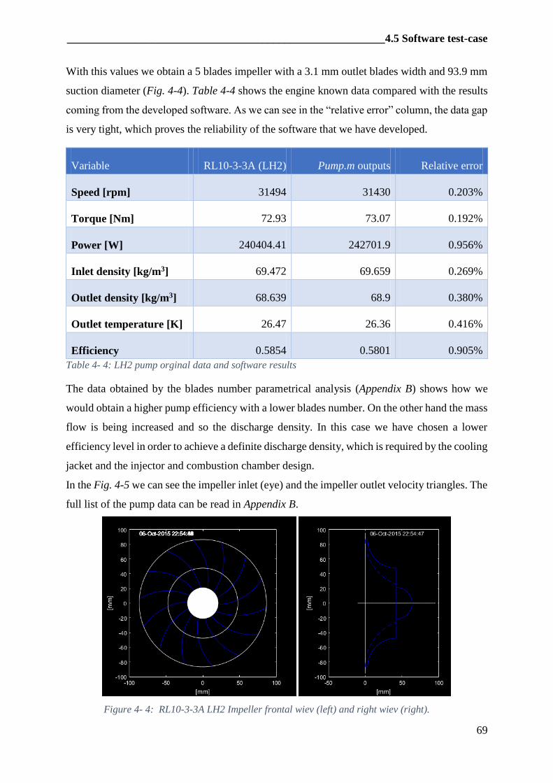
_________________________________________________________ 4.5 Software test-case

69

With this values we obtain a 5 blades impeller with a 3.1 mm outlet blades width and 93.9 mm

suction diameter (Fig. 4-4). Table 4-4 shows the engine known data compared with the results

coming from the developed software. As we can see in the “relative error” column, the data gap

is very tight, which proves the reliability of the software that we have developed.

Variable RL10-3-3A (LH2)

33A3

Pump.m outputs Relative error

Speed [rpm] 31494 31430 0.203%

Torque [Nm] 72.93 73.07 0.192%

Power [W] 240404.41 242701.9 0.956%

Inlet density [kg/m3] 69.472 69.659

4

0.269%

Outlet density [kg/m3] 68.639 68.9 0.380%

Outlet temperature [K] 26.47 26.36 0.416%

Efficiency 0.5854 0.5801 0.905%

Table 4- 4: LH2 pump orginal data and software results

The data obtained by the blades number parametrical analysis (Appendix B) shows how we

would obtain a higher pump efficiency with a lower blades number. On the other hand the mass

flow is being increased and so the discharge density. In this case we have chosen a lower

efficiency level in order to achieve a definite discharge density, which is required by the cooling

jacket and the injector and combustion chamber design.

In the Fig. 4-5 we can see the impeller inlet (eye) and the impeller outlet velocity triangles. The

full list of the pump data can be read in Appendix B.

Figure 4- 4: RL10-3-3A LH2 Impeller frontal wiev (left) and right wiev (right).

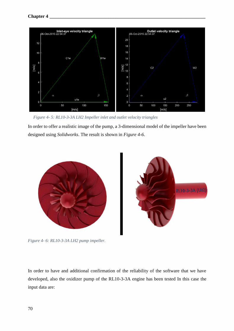
Chapter 4 __________________________________________________________________

70

Figure 4- 5: RL10-3-3A LH2 Impeller inlet and outlet velocity triangles

In order to offer a realistic image of the pump, a 3-dimensional model of the impeller have been

designed using Solidworks. The result is shown in Figure 4-6.

Figure 4- 6: RL10-3-3A LH2 pump impeller.

In order to have and additional confirmation of the reliability of the software that we have

developed, also the oxidizer pump of the RL10-3-3A engine has been tested In this case the

input data are:

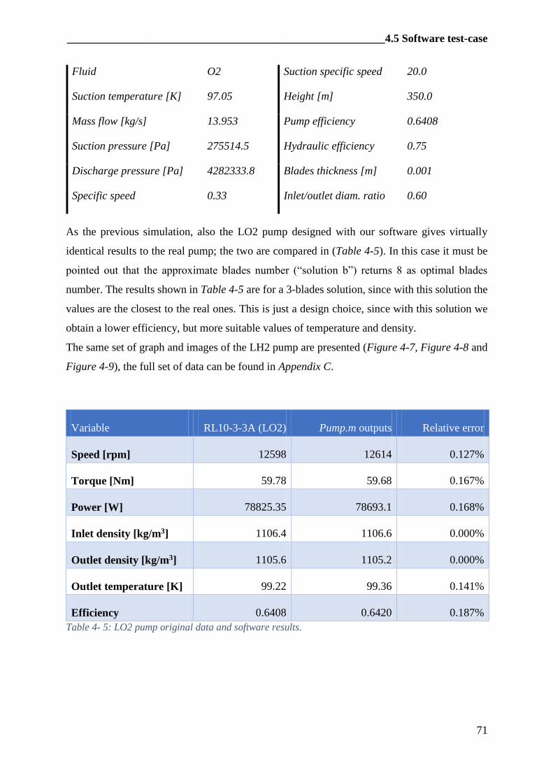
_________________________________________________________ 4.5 Software test-case

71

Fluid O2 Suction specific speed 20.0

Suction temperature [K] 97.05 Height [m] 350.0

Mass flow [kg/s] 13.953 Pump efficiency 0.6408

Suction pressure [Pa] 275514.5 Hydraulic efficiency 0.75

Discharge pressure [Pa] 4282333.8 Blades thickness [m] 0.001

Specific speed 0.33 Inlet/outlet diam. ratio 0.60

As the previous simulation, also the LO2 pump designed with our software gives virtually

identical results to the real pump; the two are compared in (Table 4-5). In this case it must be

pointed out that the approximate blades number (“solution b”) returns 8 as optimal blades

number. The results shown in Table 4-5 are for a 3-blades solution, since with this solution the

values are the closest to the real ones. This is just a design choice, since with this solution we

obtain a lower efficiency, but more suitable values of temperature and density.

The same set of graph and images of the LH2 pump are presented (Figure 4-7, Figure 4-8 and

Figure 4-9), the full set of data can be found in Appendix C.

Variable RL10-3-3A (LO2)

33A3

Pump.m outputs Relative error

Speed [rpm] 12598 12614 0.127%

Torque [Nm] 59.78 59.68 0.167%

Power [W] 78825.35 78693.1 0.168%

Inlet density [kg/m3] 1106.4 1106.6

4

0.000%

Outlet density [kg/m3] 1105.6 1105.2 0.000%

Outlet temperature [K] 99.22 99.36 0.141%

Efficiency 0.6408 0.6420 0.187%

Table 4- 5: LO2 pump original data and software results.

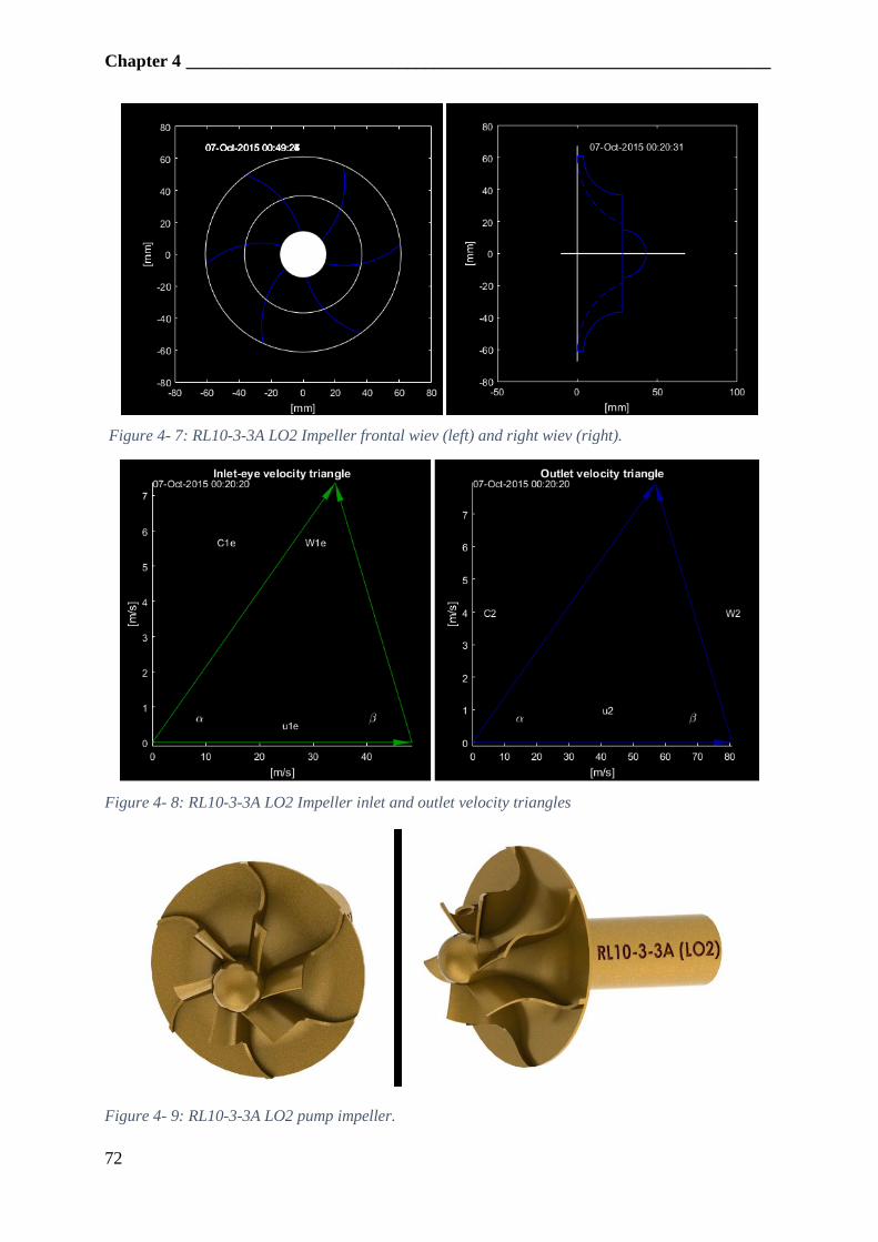
Chapter 4 __________________________________________________________________

72

Figure 4- 7: RL10-3-3A LO2 Impeller frontal wiev (left) and right wiev (right).

Figure 4- 8: RL10-3-3A LO2 Impeller inlet and outlet velocity triangles

Figure 4- 9: RL10-3-3A LO2 pump impeller.

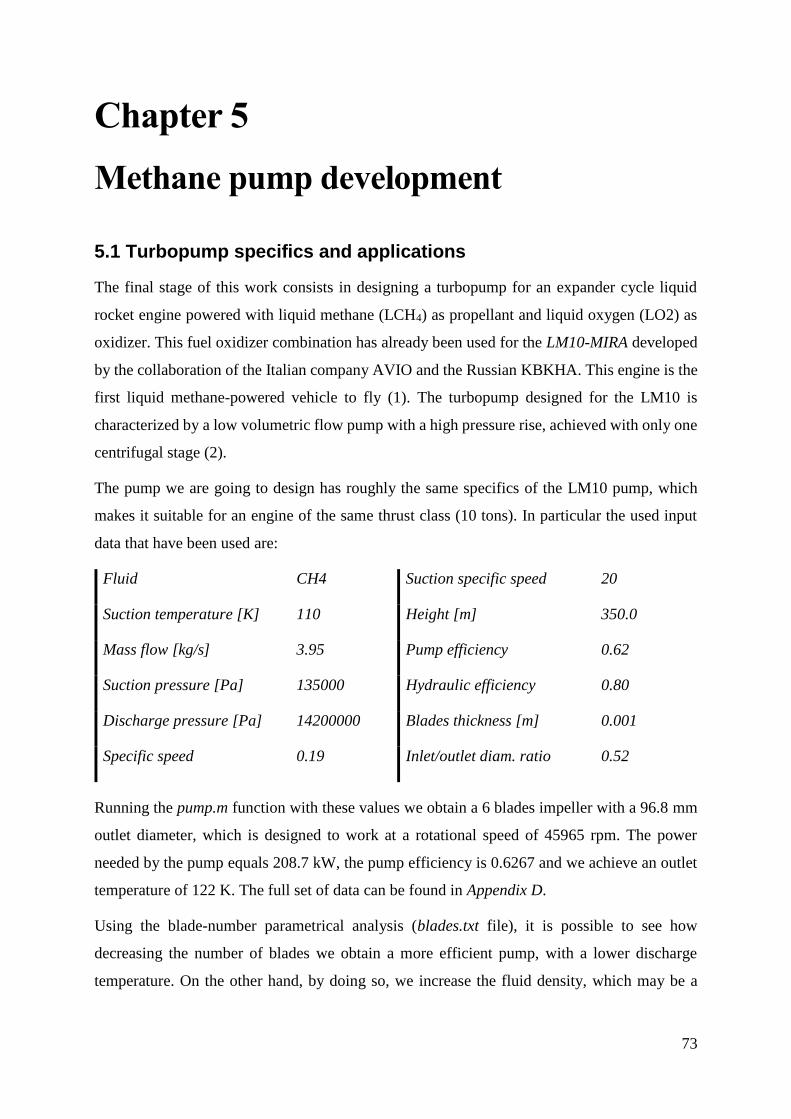
73

Chapter 5

Methane pump development

5.1 Turbopump specifics and applications

The final stage of this work consists in designing a turbopump for an expander cycle liquid

rocket engine powered with liquid methane (LCH4) as propellant and liquid oxygen (LO2) as

oxidizer. This fuel oxidizer combination has already been used for the LM10-MIRA developed

by the collaboration of the Italian company AVIO and the Russian KBKHA. This engine is the

first liquid methane-powered vehicle to fly (1). The turbopump designed for the LM10 is

characterized by a low volumetric flow pump with a high pressure rise, achieved with only one

centrifugal stage (2).

The pump we are going to design has roughly the same specifics of the LM10 pump, which

makes it suitable for an engine of the same thrust class (10 tons). In particular the used input

data that have been used are:

Fluid CH4 Suction specific speed 20

Suction temperature [K] 110 Height [m] 350.0

Mass flow [kg/s] 3.95 Pump efficiency 0.62

Suction pressure [Pa] 135000 Hydraulic efficiency 0.80

Discharge pressure [Pa] 14200000 Blades thickness [m] 0.001

Specific speed 0.19 Inlet/outlet diam. ratio 0.52

Running the pump.m function with these values we obtain a 6 blades impeller with a 96.8 mm

outlet diameter, which is designed to work at a rotational speed of 45965 rpm. The power

needed by the pump equals 208.7 kW, the pump efficiency is 0.6267 and we achieve an outlet

temperature of 122 K. The full set of data can be found in Appendix D.

Using the blade-number parametrical analysis (blades.txt file), it is possible to see how

decreasing the number of blades we obtain a more efficient pump, with a lower discharge

temperature. On the other hand, by doing so, we increase the fluid density, which may be a

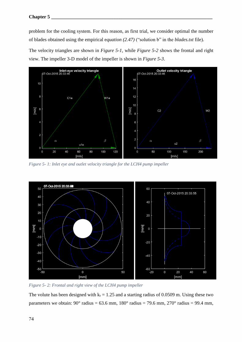
Chapter 5 __________________________________________________________________

74

problem for the cooling system. For this reason, as first trial, we consider optimal the number

of blades obtained using the empirical equation (2.47) (“solution b” in the blades.txt file).

The velocity triangles are shown in Figure 5-1, while Figure 5-2 shows the frontal and right

view. The impeller 3-D model of the impeller is shown in Figure 5-3.

Figure 5- 1: Inlet eye and outlet velocity triangle for the LCH4 pump impeller

Figure 5- 2: Frontal and right view of the LCH4 pump impeller

The volute has been designed with kr = 1.25 and a starting radius of 0.0509 m. Using these two

parameters we obtain: 90° radius = 63.6 mm, 180° radius = 79.6 mm, 270° radius = 99.4 mm,

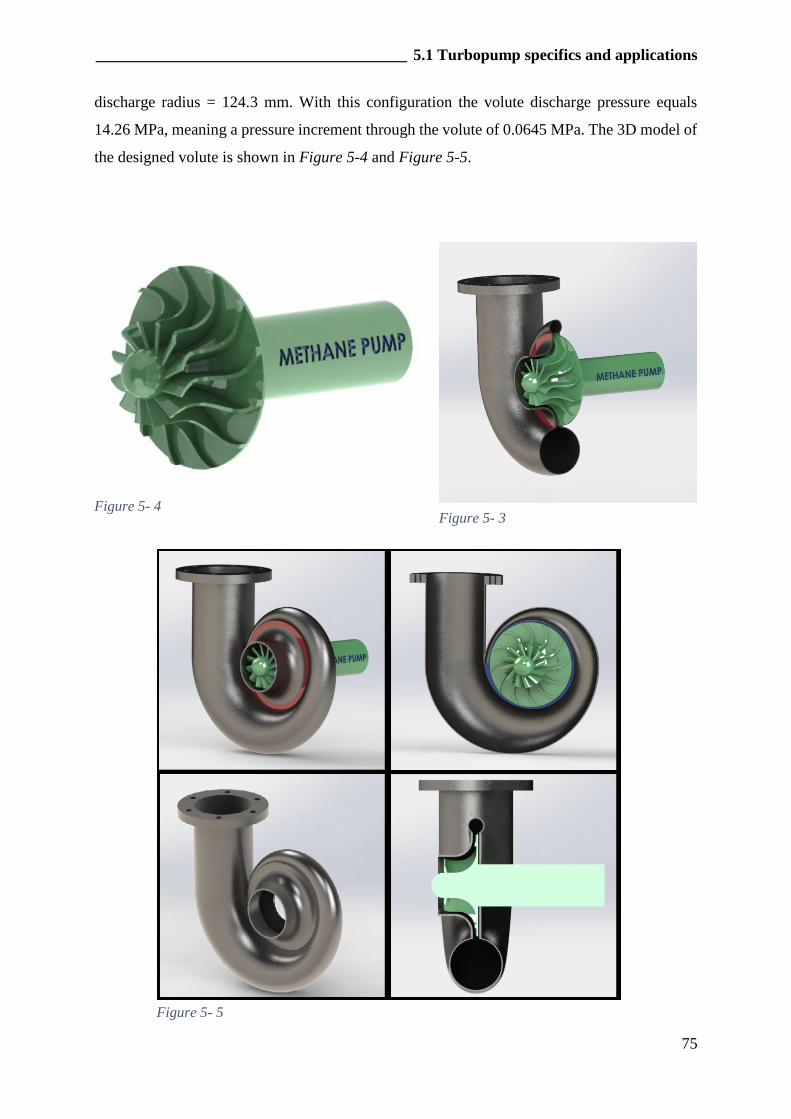
_______________________________________ 5.1 Turbopump specifics and applications

75

discharge radius = 124.3 mm. With this configuration the volute discharge pressure equals

14.26 MPa, meaning a pressure increment through the volute of 0.0645 MPa. The 3D model of

the designed volute is shown in Figure 5-4 and Figure 5-5.

Figure 5- 4 Figure 5- 3

Figure 5- 5

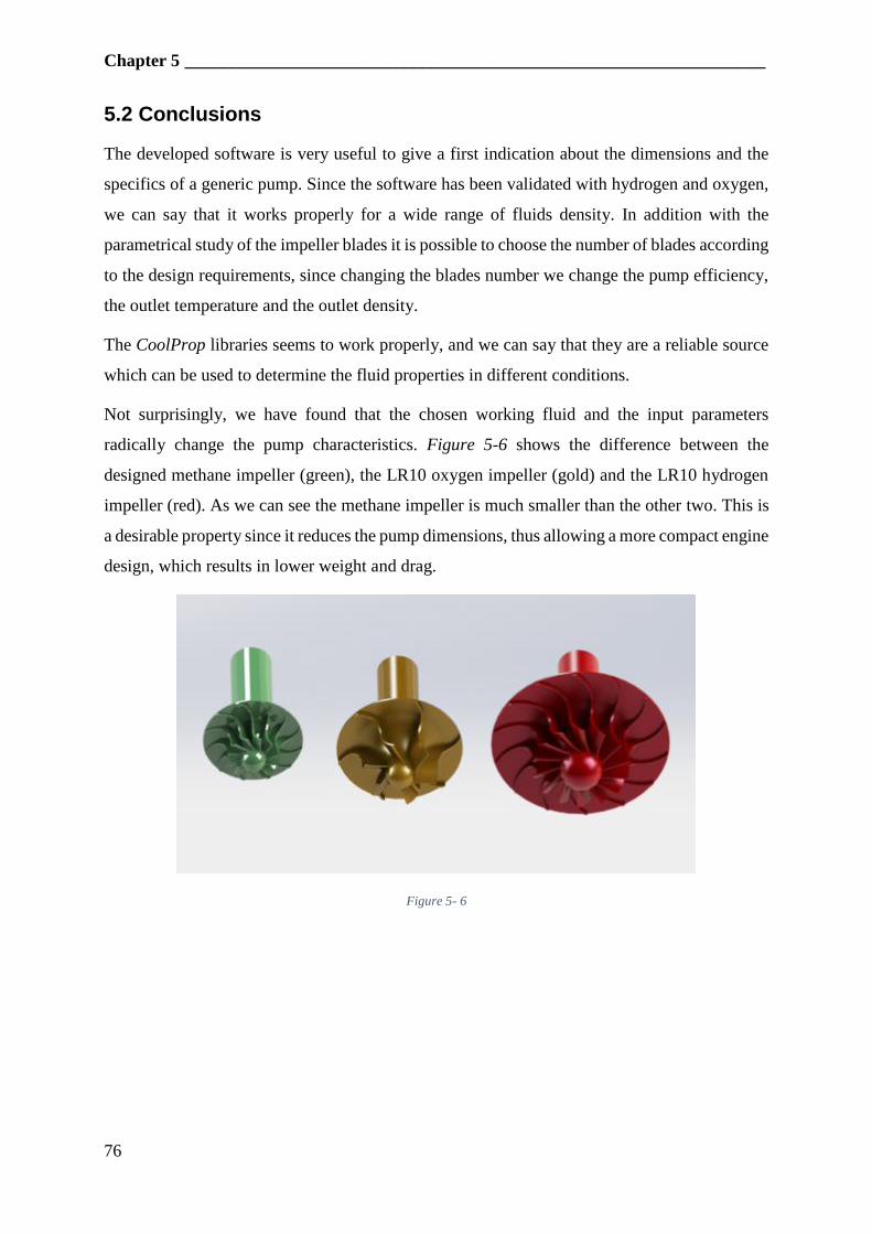
Chapter 5 __________________________________________________________________

76

5.2 Conclusions

The developed software is very useful to give a first indication about the dimensions and the

specifics of a generic pump. Since the software has been validated with hydrogen and oxygen,

we can say that it works properly for a wide range of fluids density. In addition with the

parametrical study of the impeller blades it is possible to choose the number of blades according

to the design requirements, since changing the blades number we change the pump efficiency,

the outlet temperature and the outlet density.

The CoolProp libraries seems to work properly, and we can say that they are a reliable source

which can be used to determine the fluid properties in different conditions.

Not surprisingly, we have found that the chosen working fluid and the input parameters

radically change the pump characteristics. Figure 5-6 shows the difference between the

designed methane impeller (green), the LR10 oxygen impeller (gold) and the LR10 hydrogen

impeller (red). As we can see the methane impeller is much smaller than the other two. This is

a desirable property since it reduces the pump dimensions, thus allowing a more compact engine

design, which results in lower weight and drag.

Figure 5- 6

77

Appendix

Appendix A – MatLab additional functions

function impellerPlot(r1, r2, rsh, beta2, rot)

whitebg('k')

set(gcf, 'color', 'k')

set(gcf, 'InvertHardCopy', 'off');

ang([0,0], r2, [0, 2*pi], 'w-'); hold on

ang([0,0], r1, [0, 2*pi], 'w-');

text(-r2, r2+r2/10, datestr(clock));

i=0;

for teta = 0:0.01:2*pi

i=i+1;

x2(i) = r2*cos(teta);

y2(i) = r2*sin(teta);

end

j=0;

i=0;

ii=0;

for ra=20:1:120

i=i+1;

delta(i) = inter(ra, x2, y2, beta2);

r(i) = ra;

end

c = delta(delta~=0);

pos=find(delta==min(c));

rFin=r(pos);

j=0;

for teta = 0:0.01:pi

j=j+1;

xa(j) = -rFin+rFin*cos(teta);

ya(j) = rFin*sin(teta);

end

[a, b] = intersections(x2, y2, xa, ya);

for j=1:(pi/0.01)

if xa(j)>a

xf(j) = xa(j);

yf(j) = ya(j);

end

end

h = plot(xf,yf, 'b');

xlabel('[mm]');

ylabel('[mm]');

Appendix _______________________________________________________________________

78

rotate(h, [0,0,1], rot); %chiamare la funzione con ciclo per far ruotare

for teta = 0:0.01:2*pi

i=i+1;

xsh(i) = rsh*cos(teta);

ysh(i) = rsh*sin(teta);

end

area(xsh,ysh, 'ShowBaseLine', 'off', 'FaceColor', 'w');

daspect([1,1,1]);

end

function impellerPlotDx(B1, B2, Dshaft, Dt2)

Rshaft = Dshaft/2;

Rt2 = Dt2 / 2;

whitebg('k')

set(gcf, 'color', 'k')

set(gcf, 'InvertHardCopy', 'off');

plot([-10, Rt2+Rt2/10],[0,0], 'color', 'w', 'LineWidth', 1); hold on

plot([0, 0], [-(Rt2+Rt2/10); Rt2+Rt2/10], 'color', 'w', 'LineWidth', 1);

text(2*B2, Rt2+Rt2/10, datestr(clock));

%superior half

plot([0, B2], [Rt2, Rt2], 'b');

i=0;

r = Rt2-(B1+Rshaft);

for teta = 0:0.01:pi/2

i=i+1;

x1(i) = r-r*cos(teta)+B2;

y1(i) = -r*sin(teta)+Rt2;

end

plot(x1, y1, 'b');

plot([r+B2, r+B2], [(B1+Rshaft), 0], 'b');

rr = Rt2-Rshaft;

i=0;

for teta = 0:0.01:pi/2

i=i+1;

x2(i) = rr-rr*cos(teta);

y2(i) = -rr*sin(teta)+Rt2;

if x2(i)<(r+B2)

xx(i) = x2(i);

yy(i) = y2(i);

__________________________________________ Appendix A – MatLab additional functions

79

end

end

plot(xx, yy, 'b--');

%area(xx, yy);

%bottom half

plot([0, B2], [-Rt2, -Rt2], 'b');

i=0;

r = Rt2-(B1+Rshaft);

for teta = 0:0.01:pi/2

i=i+1;

x1(i) = r-r*cos(teta)+B2;

y1(i) = +r*sin(teta)-Rt2;

end

plot(x1, y1, 'b');

plot([r+B2, r+B2], [-(B1+Rshaft), 0], 'b');

rr = Rt2-Rshaft;

i=0;

for teta = 0:0.01:pi/2

i=i+1;

x2(i) = rr-rr*cos(teta);

y2(i) = rr*sin(teta)-Rt2;

if x2(i)<(r+B2)

xxb(i) = x2(i);

yyb(i) = y2(i);

end

end

plot(xxb, yyb, 'b--');

%Shaft

i=0;

for teta = 0:0.01:pi

i=i+1;

x(i) = Rshaft*sin(teta)+r+B2;

y(i) = Rshaft*cos(teta);

end

plot(x, y, 'b');

xlabel('[mm]');

ylabel('[mm]');

daspect([1,1,1]);

hold off

end

function delta = inter(ra, x2, y2, beta2)

j=0;

for teta = 0:0.01:pi

j=j+1;

Appendix _______________________________________________________________________

80

xa(j) = -ra+ra*cos(teta);

ya(j) = ra*sin(teta);

end

%plot(xa,ya);

[a, b] = intersections(x2, y2, xa, ya);

if a~=0

[xai, xaiPos] = min(abs(a-xa));

xa(xaiPos);

betaA=abs(atan((ya(xaiPos)-ya(xaiPos-1))/(xa(xaiPos)-xa(xaiPos-1))));

delta = abs(beta2-betaA);

else

delta = 0;

end

end

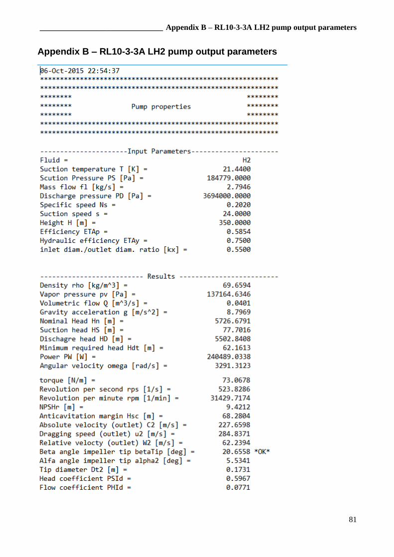
_______________________________ Appendix B – RL10-3-3A LH2 pump output parameters

81

Appendix B – RL10-3-3A LH2 pump output parameters

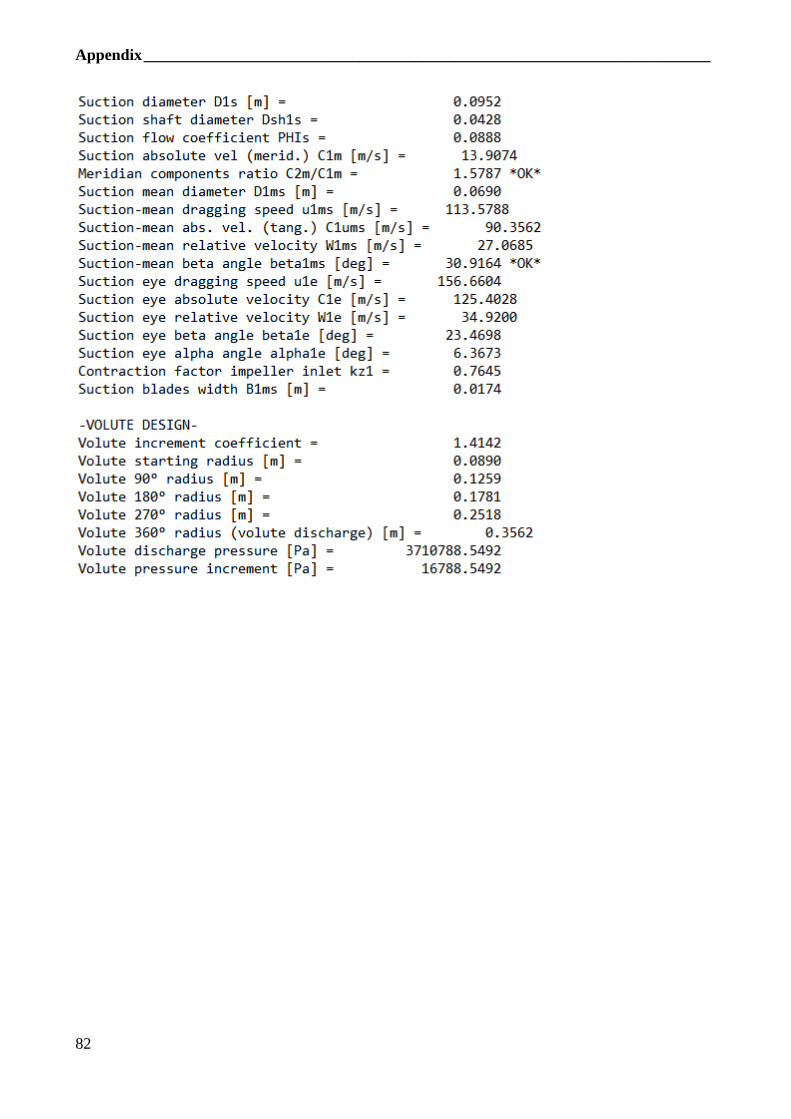
Appendix _______________________________________________________________________

82

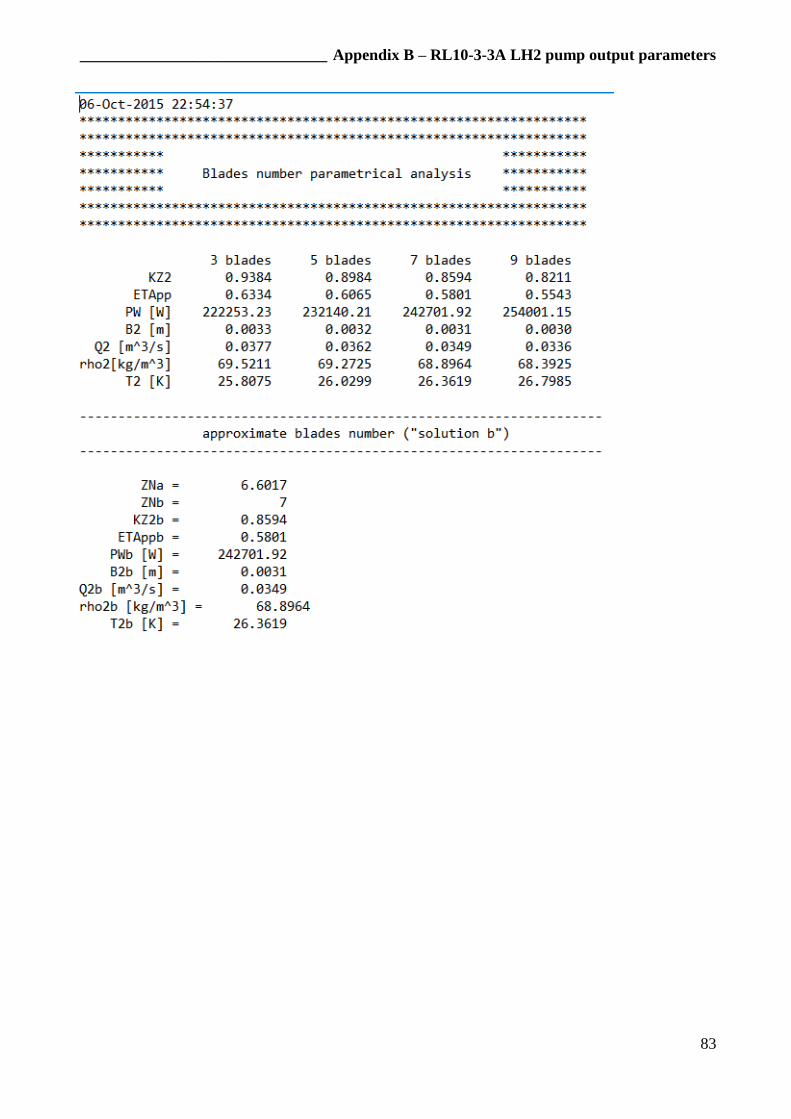
_______________________________ Appendix B – RL10-3-3A LH2 pump output parameters

83

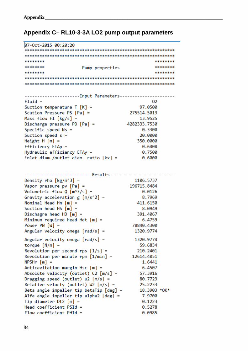
Appendix _______________________________________________________________________

84

Appendix C– RL10-3-3A LO2 pump output parameters

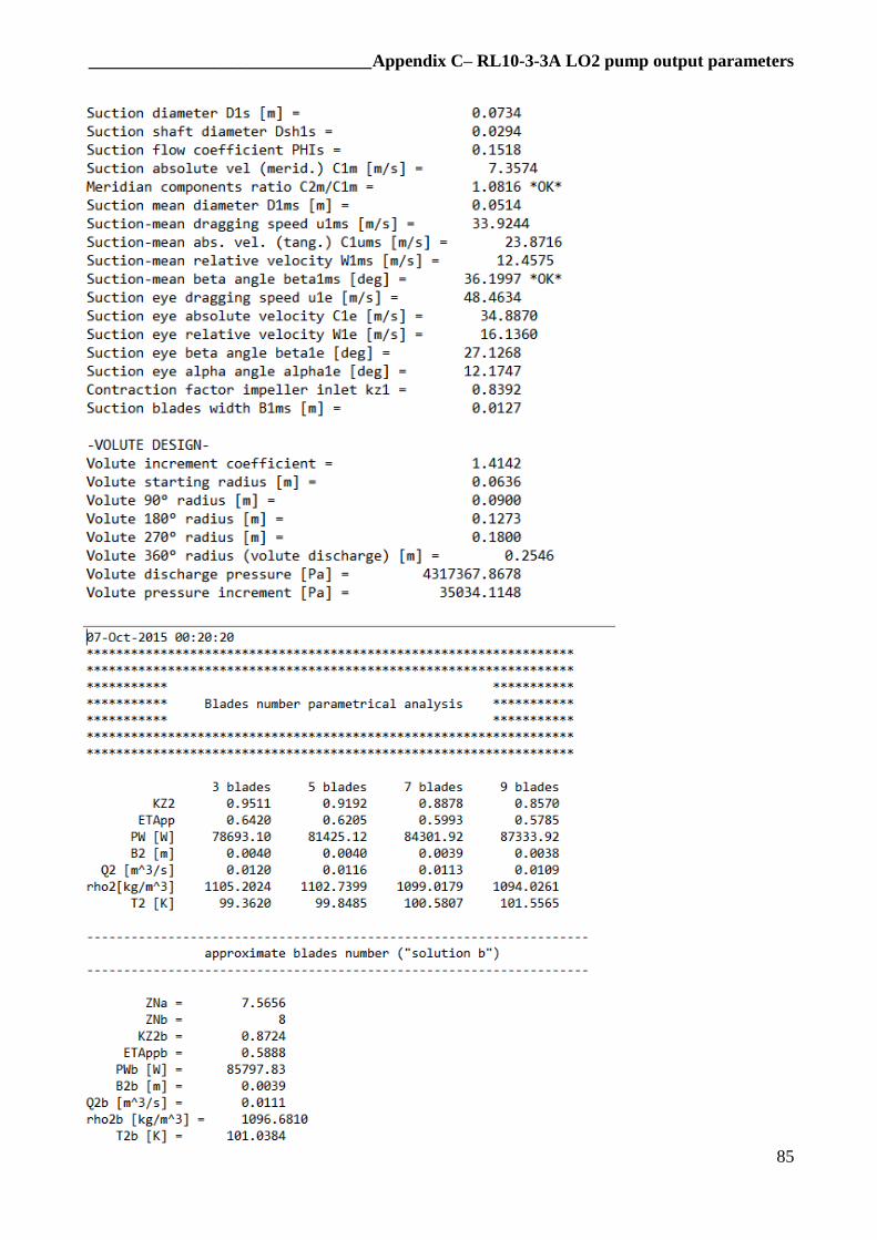
________________________________ Appendix C– RL10-3-3A LO2 pump output parameters

85

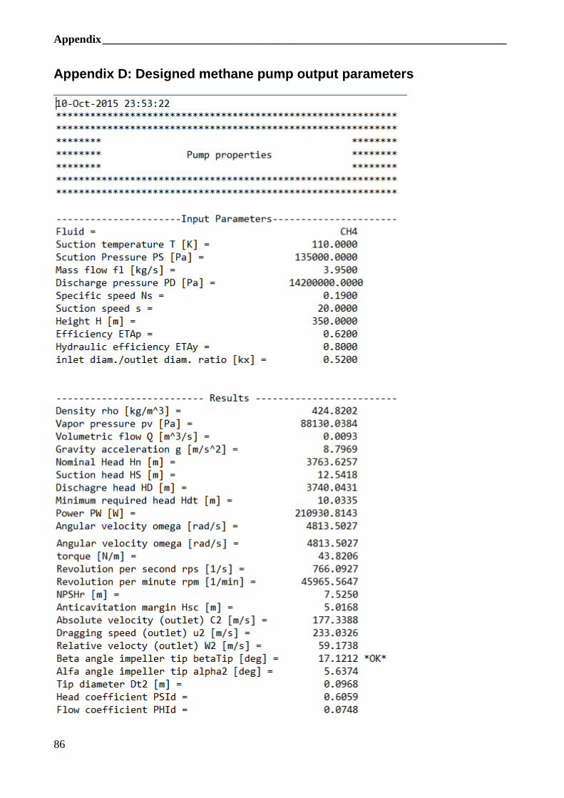
Appendix _______________________________________________________________________

86

Appendix D: Designed methane pump output parameters

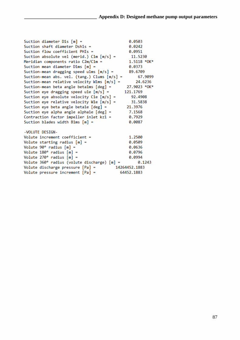
______________________________ Appendix D: Designed methane pump output parameters

87

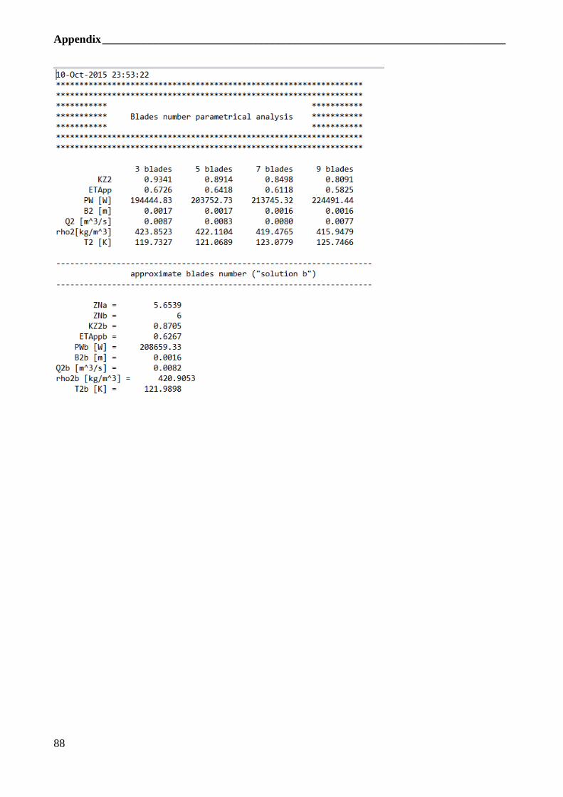
Appendix _______________________________________________________________________

88

89

References

1. Strain, William S. Design of an oxygen turbopump for a dual expander rocket engine. 2008.

2. Sutton, George P. Rocket propulsion elements (7th edition).

3. Huang, Dieter K. Huzel - David H. Modern engineering for design of liquid propellant rocket

engines.

4. Sexton, Gabriel L. Johnson - Thomas D. Johnson sexton cycle rocket engine patent.

5. Limerick, Charles D. METHOD AND APPARATUS FOR INCREASING COMBUSTION

CHAMBER PRESSURE IN A HIGH PRESSURE EXPANDER CYCLE ROCKET ENGINE. 5,410,874

USA, 02 05 1995.

6. NASA contractor report 187217 - Advanced engine study program. Masters, D.E. Galler, T.F.

Denman, R.A. Shied, J.R. Black. 1993.

7. SANTIAGO, JORGE R. Evolution of the RL10 liquid rocket engine for a new upperstage

application.

8. Mitsubishi Heavy Industries Technical Review Vol. 48 No. 4. ONGA, M. ATSUMI - K.

YOSHIKAWA - A. OGAWARA - T. 2011.

9. Cannon, James L. Liquid Propulsion: Propellant Feed System Design. Encyclopedia of Aerospace

Engineering, Volume 2 Propulsion & Power, Wiley Publishers.

10. Leto, A. Turbopump design methods for liquid rocket engine.

11. Huang, Dieter K. Huzel - David H. MOdern engineerinf for design of liquid-propellant rocket

engines. 1992.

12. Wright, Terry. Fluid Machinery: Performance, Analysis, and Design.

13. Cooper, I. J. Karassik - J. P. Messina - P. Pump Handbook.

14. Centrifugal pumps design and application - 2nd edition. Ross, V. S. Lobanoff - R. R. 1992.

15. Effect of relative impeller-to-volute position on hydraulic efficiency and static radial force

distribution in a circular volute centrifugal pump. D. O. Baun, R. D. Flack, L. Kostner. s.l. : ASME

Journal of Fluids Engineering, 2000.

16. Effect of volute design and number of impeller blades on laterla impeller forces and hydraulic

performances. D. O. Baun, R. D. Flack. 2003.

References ______________________________________________________________________

90

17. huang, Huzel and. Design of liquid propellants rocket engines.

18. [Online] www.coolprop.org.

19. [Online] http://www.coolprop.org/coolprop/HighLevelAPI.html#parameter-table.

20. Copyright (c) 2002, Tom Davis -

http://www.mathworks.com/matlabcentral/fileexchange/14056-arrow3-version-5. [Online]

21. Binder, Michael P. A transient model of the RL10A-3-3A rocket engine.

22. http://www.caeconference.com/proceedings/abstract/abstract_08/avio_cira_cfx.html.

[Online]

23. FUel turbopump development for the LM10-MIRA LOx-LNG expander cycle enginein the

frame of the LYRA program. M. Rudnykh, G. Cagiano, A.G. Kravchenko, S.V. Chembartsev,

A. De Lillis, E. D'Anversa.