UNIVERSITÄTSBIBLIOTHEK BRAUNSCHWEIG · time the train runs through the braking distance that is signaled by the cab signal system. Drawing the blocking times of all block sections

UNIVERSITÄTSBIBLIOTHEK BRAUNSCHWEIG

Jörn Pachl, Thomas White ANALYTICAL CAPACITY MANAGEMENT WITH BLOCKING TIMES URL: http://www.digibib.tu-bs.de/?docid=00015768 Zuerst erschienen in: Transportation Research Board : 83rd Annual Meeting on January 11-15, 2004. Compendium of Papers CD-ROM HINWEIS: Dieser elektronische Text wird hier nicht in der offiziellen Form wiedergegeben, in der er in der Originalversion erschienen ist. Es gibt keine inhaltlichen Unterschiede zwischen den beiden Erscheinungsformen des Aufsatzes; es kann aber Unterschiede in den Zeilen- und Seitenumbrüchen geben.

Joern Pachl, Thomas White

1

ANALYTICAL CAPACITY MANAGEMENT WITH BLOCKING TIMES 4062 words 13 figures

AUTHORS Prof. Dr. Joern Pachl Technical University Braunschweig, Institute of Railway Systems Engineering and Traffic Safety Pockelsstrasse 3, D-38106 Braunschweig, Germany Phone: 49 531 391 3380, Fax: 49 531 391 5955, email: [email protected] Thomas White Transit Safety Management 3604 220th Place SW, Mountlake Terrace, WA 98043, USA Phone: 1 425 771 4289, Fax: 1 888 694 4798, email: [email protected]

http://www.digibib.tu-bs.de/?docid=00015768 21/11/2006


2

ABSTRACT Analytical capacity research is an important infrastructure and operations planning tool that can be used alone or in conjunction with simulation. The blocking time theory is a new approach in analytical capacity research. The blocking time is the total elapsed time a section of track is exclusively allocated to a train and therefore blocked for other trains. Calculating blocking times and producing blocking time diagrams leads to a very detailed evaluation of the capacity and exploitation of a railroad line. It also shows very clearly how the capacity depends upon the signaling system. Beside capacity research, blocking time analysis is also a great tool to support computer-based scheduling. Although originally developed for European railroads, blocking time analysis has now found first applications in North American railroad industry.



3

METHODS FOR CAPACITY MANAGEMENT Methods for capacity research of railroad lines may be divided in two classes: • analytical research • simulation

Analytical research is the traditional method of capacity research. It is conducted by calculation of minimum headways and exploitation rates from the infrastructure and timetable characteristics to determine and describe the capacity of a line or other parts of a railroad network. Simulation follows the experimental method of natural science instead. The experiments are done in a computer model by simulating the running operation and measuring data [mostly delays] to evaluate the capacity. In recent years simulation models have become very popular and have replaced analytical methods in many fields of capacity research. However, a new approach has renewed interest in analytical capacity research. This new approach is called blocking time analysis.

Before explaining how it works, a short look at the advantages and weaknesses of capacity research with blocking times is provided. A big advantage of capacity analysis with blocking times is the detailed evaluation of the exploitation of a line or sections of a line. Very clear diagrams show the exploitation of a line and allow a clear determination of the timetable capacity. An exact location of critical points where delays will be transmitted between trains is also possible. With simulation, this is often a problem. A simulation will produce delay statistics in many ways, but it is often not an easy task to find the points of the infrastructure that are responsible for the delays. With blocking time analysis, for layouts with moderate complexity, there is less effort to build the model than with simulation. In North America this applies to most railroad infrastructure outside of big terminal areas. The effort to build the model will increase superproportionally with the complexity of the layout, however. Methods for blocking time analysis can also be integrated as an add-on to simulation programs for a better presentation and evaluation of simulation results. The weakness of blocking time analysis is that it works only on the scheduling level but there is no evaluation of running operation. Thus, promoting blocking time analysis is in no way intented to argue against simulation. The best results will be achieved by combining both methods. For this reason, in recent years blocking time modules have been added to a number of simulation programs (1).

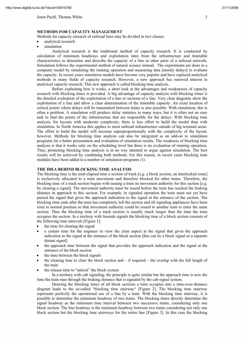
THE IDEA BEHIND BLOCKING TIME ANALYSIS The blocking time is the total elapsed time a section of track [e.g. a block section, an interlocked route] is exclusively allocated to a train movement and therefore blocked for other trains. Therefore, the blocking time of a track section begins with issuing a train its movement authority for this section [e.g. by clearing a signal]. The movement authority must be issued before the train has reached the braking distance in approach to this section. For example, in signaled operation the train must not yet have passed the signal that gives the approach indication to the signal at the entrance of the section. The blocking time ends after the train has completely left the section and all signaling appliances have been reset to normal position so that movement authority could be issued to another train to enter the same section. Thus the blocking time of a track section is usually much longer than the time the train occupies the section. In a territory with lineside signals the blocking time of a block section consists of the following time intervals [Figure 1]: • the time for clearing the signal • a certain time for the engineer to view the clear aspect at the signal that gives the approach

indication to the signal at the entrance of the block section [this can be a block signal or a separate distant signal]

• the approach time between the signal that provides the approach indication and the signal at the entrance of the block section

• the time between the block signals • the clearing time to clear the block section and – if required – the overlap with the full length of

the train • the release time to “unlock” the block system

In a territory with cab signaling, the principle is quite similar but the approach time is now the time the train runs through the braking distance that is signaled by the cab signal system.

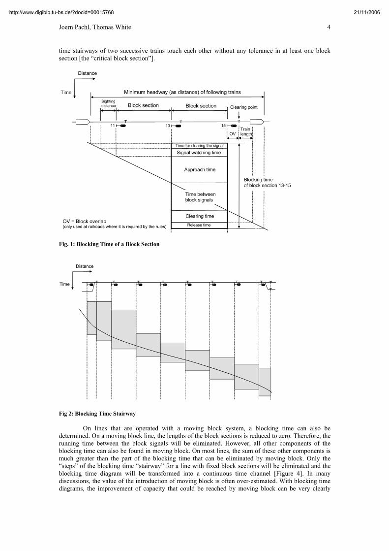
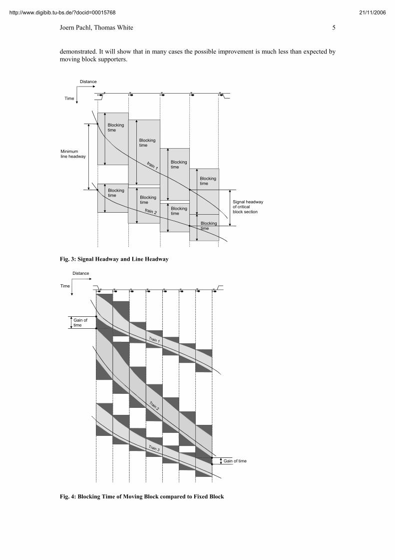
Drawing the blocking times of all block sections a train occupies into a time-over-distance diagram leads to the so-called “blocking time stairway“ [Figure 2]. The blocking time stairway represents perfectly the operational use of a line by a train. With the blocking time stairway, it is possible to determine the minimum headway of two trains. The blocking times directly determine the signal headway as the minimum time interval between two successive trains, considering only one block section. The line headway is the minimum headway between two trains considering not only one block section but the blocking time stairways for the entire line [Figure 3]. In this case the blocking



4

time stairways of two successive trains touch each other without any tolerance in at least one block section [the “critical block section”].

Block section

11 13

Clearing point

Minimum headway (as distance) of following trains

Trainlength

Sighting distance

Blocking timeof block section 13-15

Approach time

Signal watching timeTime for clearing the signal

Clearing time

Release time

Time between block signals

15

Block section

Time

Distance

OV

OV = Block overlap (only used at railroads where it is required by the rules)

Fig. 1: Blocking Time of a Block Section

Time

Distance

Fig 2: Blocking Time Stairway

On lines that are operated with a moving block system, a blocking time can also be determined. On a moving block line, the lengths of the block sections is reduced to zero. Therefore, the running time between the block signals will be eliminated. However, all other components of the blocking time can also be found in moving block. On most lines, the sum of these other components is much greater than the part of the blocking time that can be eliminated by moving block. Only the “steps” of the blocking time “stairway” for a line with fixed block sections will be eliminated and the blocking time diagram will be transformed into a continuous time channel [Figure 4]. In many discussions, the value of the introduction of moving block is often over-estimated. With blocking time diagrams, the improvement of capacity that could be reached by moving block can be very clearly



5

demonstrated. It will show that in many cases the possible improvement is much less than expected by moving block supporters.

Blocking time

Blocking time

Blocking time

Blocking time

Blocking time Blocking

timeBlocking time

Blocking time

Minimumline headway

Signal headwayof critical block section

train 1

train 2

Time

Distance

Fig. 3: Signal Headway and Line Headway

Train 1

Train 2

Train 3

Gain of time

Gain of time

Time

Distance

Fig. 4: Blocking Time of Moving Block compared to Fixed Block



6

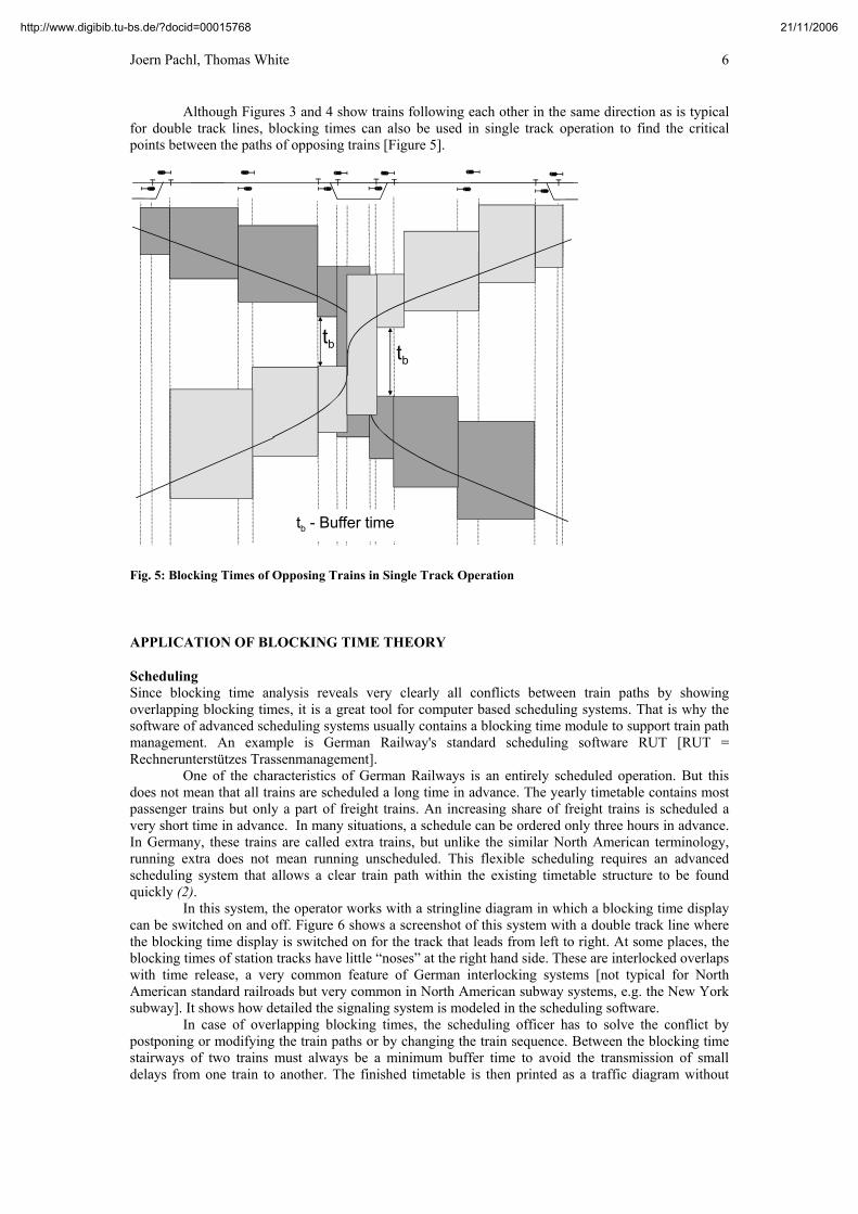
Although Figures 3 and 4 show trains following each other in the same direction as is typical for double track lines, blocking times can also be used in single track operation to find the critical points between the paths of opposing trains [Figure 5].

tb

tb

tb - Buffer time

Fig. 5: Blocking Times of Opposing Trains in Single Track Operation

APPLICATION OF BLOCKING TIME THEORY

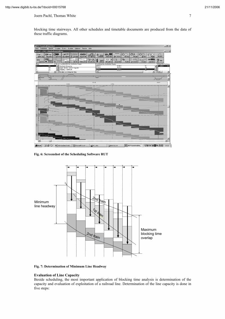
Scheduling Since blocking time analysis reveals very clearly all conflicts between train paths by showing overlapping blocking times, it is a great tool for computer based scheduling systems. That is why the software of advanced scheduling systems usually contains a blocking time module to support train path management. An example is German Railway's standard scheduling software RUT [RUT = Rechnerunterstützes Trassenmanagement].

One of the characteristics of German Railways is an entirely scheduled operation. But this does not mean that all trains are scheduled a long time in advance. The yearly timetable contains most passenger trains but only a part of freight trains. An increasing share of freight trains is scheduled a very short time in advance. In many situations, a schedule can be ordered only three hours in advance. In Germany, these trains are called extra trains, but unlike the similar North American terminology, running extra does not mean running unscheduled. This flexible scheduling requires an advanced scheduling system that allows a clear train path within the existing timetable structure to be found quickly (2).

In this system, the operator works with a stringline diagram in which a blocking time display can be switched on and off. Figure 6 shows a screenshot of this system with a double track line where the blocking time display is switched on for the track that leads from left to right. At some places, the blocking times of station tracks have little “noses” at the right hand side. These are interlocked overlaps with time release, a very common feature of German interlocking systems [not typical for North American standard railroads but very common in North American subway systems, e.g. the New York subway]. It shows how detailed the signaling system is modeled in the scheduling software.

In case of overlapping blocking times, the scheduling officer has to solve the conflict by postponing or modifying the train paths or by changing the train sequence. Between the blocking time stairways of two trains must always be a minimum buffer time to avoid the transmission of small delays from one train to another. The finished timetable is then printed as a traffic diagram without



7

blocking time stairways. All other schedules and timetable documents are produced from the data of these traffic diagrams.

Fig. 6: Screenshot of the Scheduling Software RUT

Train 2

Train 3

Train 3

Minimumline headway

2nd train

2nd train

1st train

Maximumblocking time overlap

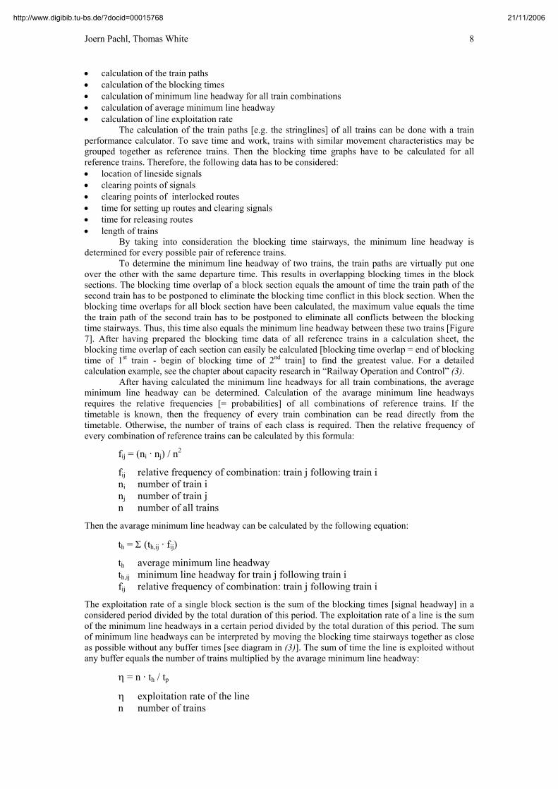
Fig. 7: Determination of Minimum Line Headway

Evaluation of Line Capacity Beside scheduling, the most important application of blocking time analysis is determination of the capacity and evaluation of exploitation of a railroad line. Determination of the line capacity is done in five steps:



8

• calculation of the train paths • calculation of the blocking times • calculation of minimum line headway for all train combinations • calculation of average minimum line headway • calculation of line exploitation rate

The calculation of the train paths [e.g. the stringlines] of all trains can be done with a train performance calculator. To save time and work, trains with similar movement characteristics may be grouped together as reference trains. Then the blocking time graphs have to be calculated for all reference trains. Therefore, the following data has to be considered: • location of lineside signals • clearing points of signals • clearing points of interlocked routes • time for setting up routes and clearing signals • time for releasing routes • length of trains

By taking into consideration the blocking time stairways, the minimum line headway is determined for every possible pair of reference trains.

To determine the minimum line headway of two trains, the train paths are virtually put one over the other with the same departure time. This results in overlapping blocking times in the block sections. The blocking time overlap of a block section equals the amount of time the train path of the second train has to be postponed to eliminate the blocking time conflict in this block section. When the blocking time overlaps for all block section have been calculated, the maximum value equals the time the train path of the second train has to be postponed to eliminate all conflicts between the blocking time stairways. Thus, this time also equals the minimum line headway between these two trains [Figure 7]. After having prepared the blocking time data of all reference trains in a calculation sheet, the blocking time overlap of each section can easily be calculated [blocking time overlap = end of blocking time of 1st train - begin of blocking time of 2nd train] to find the greatest value. For a detailed calculation example, see the chapter about capacity research in “Railway Operation and Control” (3).

After having calculated the minimum line headways for all train combinations, the average minimum line headway can be determined. Calculation of the avarage minimum line headways requires the relative frequencies [= probabilities] of all combinations of reference trains. If the timetable is known, then the frequency of every train combination can be read directly from the timetable. Otherwise, the number of trains of each class is required. Then the relative frequency of every combination of reference trains can be calculated by this formula: fij = (ni · nj) / n2

fij relative frequency of combination: train j following train i

ni number of train i nj number of train j n number of all trains Then the avarage minimum line headway can be calculated by the following equation: th = Σ (th,ij · fij) th average minimum line headway th,ij minimum line headway for train j following train i

fij relative frequency of combination: train j following train i The exploitation rate of a single block section is the sum of the blocking times [signal headway] in a considered period divided by the total duration of this period. The exploitation rate of a line is the sum of the minimum line headways in a certain period divided by the total duration of this period. The sum of minimum line headways can be interpreted by moving the blocking time stairways together as close as possible without any buffer times [see diagram in (3)]. The sum of time the line is exploited without any buffer equals the number of trains multiplied by the avarage minimum line headway: η = n · th / tp η exploitation rate of the line n number of trains



9

th average minimum line headway tp total elapsed time of the considered period From the experience of European railroads [mostly double track with mixed traffic of passenger and freight trains], for a good quality of operation, the line exploitation rate should not significantly exceed: • 50% during 24 hours • 80% during a peak period of 4 hours

That means the average buffer time between two trains should not be a lot less than the average minimum line headway. On single track lines with big distances between the scheduled meeting stations and on double track lines with low speed differences [e.g. electric city railways] a higher exploitation rate can be accepted. On North American railroads, these limits may differ due to different operating conditions [infrequent passenger operation, many single track lines, infrequent sidings].

On single track lines, the required buffer significantly depends on the distance between sidings in comparison with the distance between scheduled meeting points. On lines with several passing tracks between the scheduled meeting stations, delay transmission from a delayed train to opposing trains may be avoided by switching the scheduled meeting point to another siding. In this situation, a smaller buffer will be required than on lines which do not have suitable sidings to change the meeting point. A similar situation is found on a double track line that has a variety of train speeds and few or no sidings for overtaking. Thus, on a line with low reserves in infrastructure high reserves in time [buffer times] will be required and vice versa.

ANALYTICAL METHODS IN PLANNING RAIL OPERATION AND INFRASTRUCTURE IN NORTH AMERICA

Operation Analytical methods were once used extensively in planning railroad operation in North America. Train Dispatchers planned movements by calculating running times and writing them in pencil on the trainsheet. The analysis included a version of blocking time analysis, because the planning included awareness of the time needed ahead of a train to avoid restrictive signal indications. Train Dispatchers and Chief Train Dispatchers performed an analysis of traffic and capacity before setting calls for train crews at terminals. Extra trains were scheduled in a manner similar to that now practiced in Germany, but without the use of computers. Timetable scheduling and analysis was also conducted with the assistance of a stringline board, a time-distance graph of a line of railroad on which times were represented by pins and train movement between the times by string stretched between the pins. Train Dispatchers still calculate meeting and passing points, but in general, analytical methods are not applied to operation to the former extent.

Infrastructure Planning The Chief Train Dispatcher’s analysis often extended to infrastructure design. With the same methods used in planning daily operation, the office of the Chief Dispatcher would provide advice on infrastructure projects intended to reduce congestion or provide for new service. In more recent times, this analysis has been performed by departments established for that purpose, generally using heuristic computer simulation and statistical analysis.

Computer simulation is a valuable tool, however the statistical results can be misleading. For example, the standard way of determining change in capacity using computer simulation is a comparison of the delays with and without the project[s] and/or traffic being tested. Analytical methods demonstrate that this method may not be accurate, especially when considering improvised train operation typical of North America.

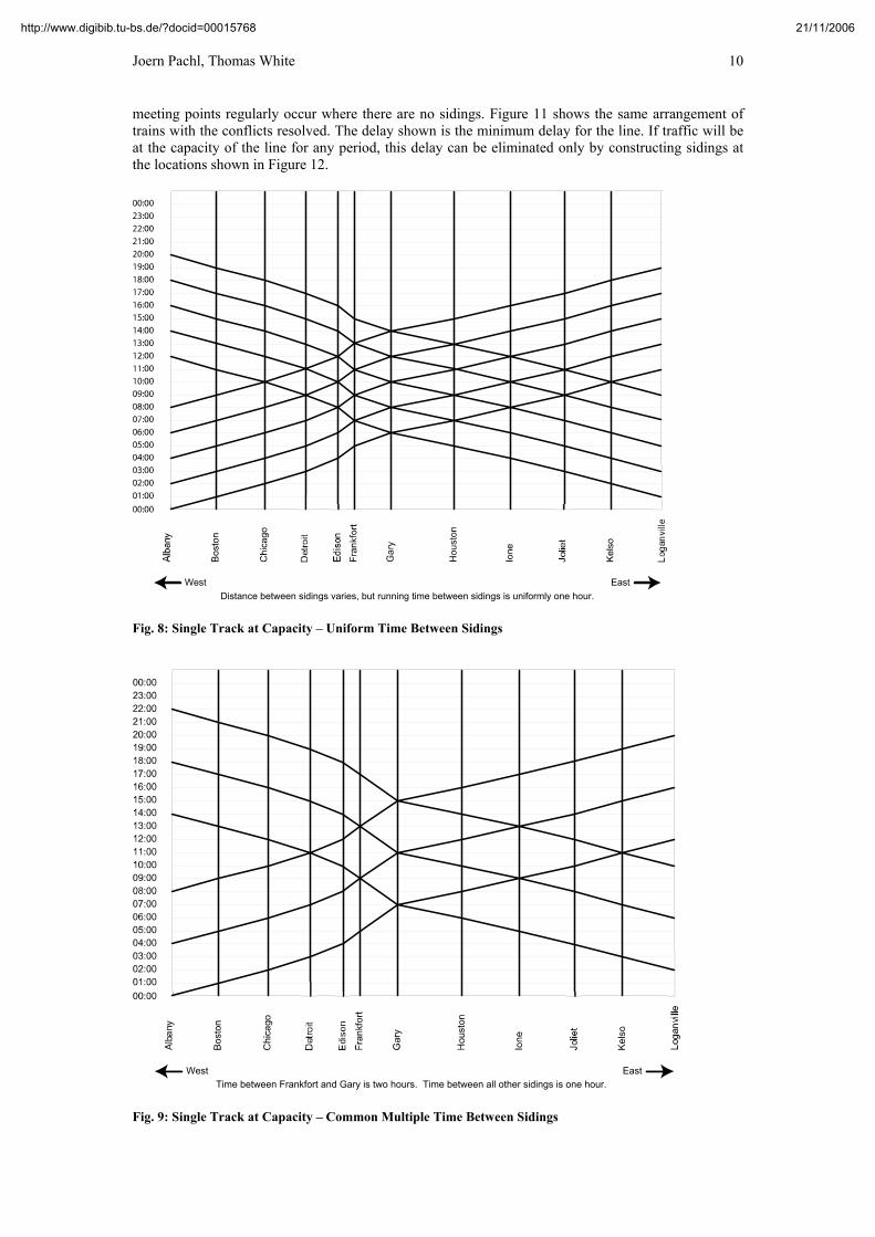
Analytical methods also demonstrate that the relationship of delay and capacity is not necessarily consistent, as shown in the following series of illustrations. Figure 8 shows a single track line with sidings one hour apart. The traffic shown is the full capacity of the line, as every movement opportunity has been used. Figure 9 shows the same line, but with the time between one pair of sidings doubled. The traffic shown is full capacity for the line, which is half of the capacity of Figure 8.

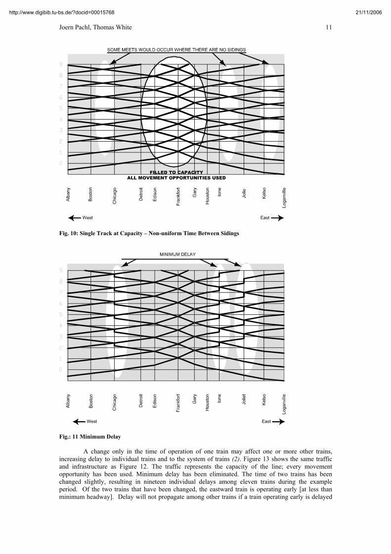
Capacity and delay may not have the expected relationship if the running time between meeting points is not uniform. The line shown in Figure 8 has uniform running time between sidings. There is no delay, although the traffic represents the full capacity of the line. The line in Figure 9 does not have uniform running time between sidings, but the running times are a common multiple. There is also no delay on this line. Figure 10 is a line with non-uniform running time between sidings. Using only running time and not conflict resolution, it can be seen that when the line is filled to capacity,



10

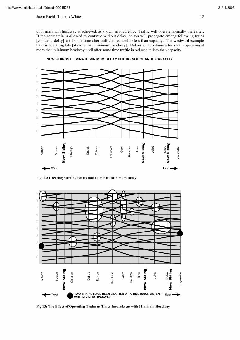
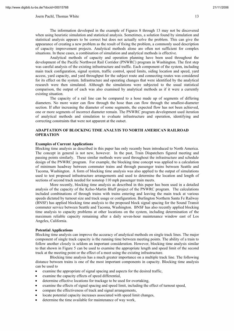
meeting points regularly occur where there are no sidings. Figure 11 shows the same arrangement of trains with the conflicts resolved. The delay shown is the minimum delay for the line. If traffic will be at the capacity of the line for any period, this delay can be eliminated only by constructing sidings at the locations shown in Figure 12.

West EastDistance between sidings varies, but running time between sidings is uniformly one hour.

Fig. 8: Single Track at Capacity – Uniform Time Between Sidings

West EastTime between Frankfort and Gary is two hours. Time between all other sidings is one hour.

Fig. 9: Single Track at Capacity – Common Multiple Time Between Sidings



11

Fig. 10: Single Track at Capacity – Non-uniform Time Between Sidings

Fig.: 11 Minimum Delay

A change only in the time of operation of one train may affect one or more other trains, increasing delay to individual trains and to the system of trains (2). Figure 13 shows the same traffic and infrastructure as Figure 12. The traffic represents the capacity of the line; every movement opportunity has been used. Minimum delay has been eliminated. The time of two trains has been changed slightly, resulting in nineteen individual delays among eleven trains during the example period. Of the two trains that have been changed, the eastward train is operating early [at less than minimum headway]. Delay will not propagate among other trains if a train operating early is delayed



12

until minimum headway is achieved, as shown in Figure 13. Traffic will operate normally thereafter. If the early train is allowed to continue without delay, delays will propagate among following trains [collateral delay] until some time after traffic is reduced to less than capacity. The westward example train is operating late [at more than minimum headway]. Delays will continue after a train operating at more than minimum headway until after some time traffic is reduced to less than capacity.

NEW SIDINGS ELIMINATE MINIMUM DELAY BUT DO NOT CHANGE CAPACITY

Fig. 12: Locating Meeting Points that Eliminate Minimum Delay

Fig 13: The Effect of Operating Trains at Times Inconsistent with Minimum Headway



13

The information developed in the example of Figures 8 through 13 may not be discovered when using heuristic simulation and statistical analysis. Sometimes, a solution found by simulation and statistical analysis appears to be correct but does not actually solve the problem. This can give the appearance of creating a new problem as the result of fixing the problem, a commonly used description of capacity improvement projects. Analytical methods alone are often not sufficient for complex situations. In these cases, a combination of simulation and analytical methods is effective.

Analytical methods of capacity and operation planning have been used throughout the development of the Pacific Northwest Rail Corridor (PNWRC) program in Washington. The first step was careful analysis of the existing infrastructure and traffic. Each component of the system, including main track configuration, signal system, traffic control, speed limits, siding location and speed, yard access, yard capacity, and yard throughput for the subject route and connecting routes was considered for its effect on the system. Infrastructure and operating changes that were identified by the analytical research were then simulated. Although the simulations were subjected to the usual statistical comparison, the output of each was also examined by analytical methods as if it were a currently existing situation.

The capacity of a rail line can be compared to a hose made up of segments of differing diameters. No more water can flow through the hose than can flow through the smallest-diameter section. If after increasing the diameter of some segments, the expected flow has not been achieved, one or more segments of incorrect diameter remain. The PNWRC program development used iteration of analytical methods and simulation to evaluate infrastructure and operation, identifying and correcting constraints that were not apparent at the outset.

ADAPTATION OF BLOCKING TIME ANALYIS TO NORTH AMERICAN RAILROAD OPERATION

Examples of Current Applications Blocking time analysis as described in this paper has only recently been introduced to North America. The concept in general is not new, however. In the past, Train Dispatchers figured meeting and passing points similarly. These similar methods were used throughout the infrastructure and schedule design of the PNWRC program. For example, the blocking time concept was applied to a calculation of minimum headway between commuter trains and through passenger trains between Seattle and Tacoma, Washington. A form of blocking time analysis was also applied to the output of simulations used to test proposed infrastructure arrangements and used to determine the location and length of sections of second track needed for nonstop 110 mph passenger train meets.

More recently, blocking time analysis as described in this paper has been used in a detailed analysis of the capacity of the Kelso-Martin Bluff project of the PNWRC program. The calculations included combinations of through trains with trains entering and leaving the main track at various speeds dictated by turnout size and track usage or configuration. Burlington Northern Santa Fe Railway (BNSF) has applied blocking time analysis to the proposed block signal spacing for the Sound Transit commuter service between Seattle and Tacoma, Washington. BNSF has also recently applied blocking time analysis to capacity problems at other locations on the system, including determination of the maximum reliable capacity remaining after a daily seven-hour maintenance window east of Los Angeles, California.

Potential Applications Blocking time analysis can improve the accuracy of analytical methods on single track lines. The major component of single track capacity is the running time between meeting points. The ability of a train to follow another closely is seldom an important consideration. However, blocking time analysis similar to that shown in Figure 5 can be used to examine the appropriate length and speed limit of the second track at the meeting point or the effect of a meet using the existing infrastructure.

Blocking time analysis has a much greater importance on a multiple track line. The following distance between trains is one of the most important components in capacity. Blocking time analysis can be used to • examine the appropriate of signal spacing and aspects for the desired traffic, • examine the capacity effects of speed differential, • determine effective locations for trackage to be used for overtaking, • examine the effects of signal spacing and speed limit, including the effect of turnout speed, • compare the effectiveness of track and signal arrangements, • locate potential capacity increases associated with speed limit changes, • determine the time available for maintenance of way work,



14

• determine the effect of maintenance of way work on capacity.

Conclusion Analytical methods including blocking time analysis can be effective for identifying and

solving capacity and reliability problems and for making the maximum use of the available infrastructure. Analytical methods combined with simulation present a more effective method of capacity research than heuristic simulation and statistical analysis. REFERENCES 1. Siefer, T.: Tasks for a Simulation Tool: Determination of Infrastructure – Capacity – Operation –

Quality. in: Implementation of Heavy Haul Technology for Network Efficiency, International Heavy Haul Association, Proceedings, Virginia Beach 2003, p. 5.53–5.60

2. Pachl, J.; White, T.: Efficiency through Integrated Planning and Operation. in: Implementation of

Heavy Haul Technology for Network Efficiency, International Heavy Haul Association, Proceedings, Virginia Beach 2003, p. 6.69–6.77

3. Pachl, J.: Railway Operation and Control. VTD Rail Publishing. Mountlake Terrace 2002


Documents

UNIVERSITÄTSBIBLIOTHEK BRAUNSCHWEIG · time the train runs through the braking distance that is signaled by the cab signal system. Drawing the blocking times of all block sections