Using airborne LiDAR to determine total sapwood area …tomo-kumagai.eco.coocan.jp/hp1501.pdf · estimating stand transpiration in plantations ... remote sensing; ... Using airborne

HYDROLOGICAL PROCESSESHydrol. Process. 29, 5071–5087 (2015)Published online 27 April 2015 in Wiley Online Library(wileyonlinelibrary.com) DOI: 10.1002/hyp.10482

Using airborne LiDAR to determine total sapwood area forestimating stand transpiration in plantations

Takami Saito,1,2* Kazukiyo Yamamoto,3 Misako Komatsu,1 Hiroki Matsuda,1 Shuji Yunohara,1

Hikaru Komatsu,4 Makiko Tateishi,1 Yang Xiang,1 Kyoichi Otsuki1 and Tomo’omi Kumagai21 Kasuya Research Forest, Kyushu University, Fukuoka 811-2415, Japan

2 Hydrospheric Atmospheric Research Center (HyARC), Nagoya University, Nagoya 464-8601, Japan3 Graduate School of Bioagricultural Sciences, Nagoya University, Nagoya 464-8601, Japan

4 The Hakubi Center for Advanced Research, Kyoto University, Kyoto 606-8302, Japan

*CCeE-mCuusiSpedermaovenumdereva

Co

Abstract:

This study offers an unprecedented opportunity to estimate total sapwood area over an entire catchment (Ascat/Ag) using small-footprint light detection and ranging technology with a minimal amount of labour in field. Forty-two-year-old plantations ofJapanese cypress (Hinoki; Chamaecyparis obtusa Sieb. et Zucc.) and Japanese cedar (Sugi; Cryptomeria japonica D. Don)vegetated the 2.98 ha experimental catchment. Field observations identified diameter at breast height (DBH) of all trees andproduced the relationship between DBH and tree sapwood area (Astre). The sum of Astre generated actual values of Ascat/Ag. Forlight detection and ranging data analyses, local maximum filtering revealed height of tree apices (H) and tree number (N) with9% omission errors. A novel process was developed to identify tree species by their apices based on height of the apices andcanopy roughness. Four methods were tested. In Methods A–C, H was converted to Astre directly or via DBH, then, the sum ofAstre created Ascat/Ag. H–Astre or H–DBH relationships were varied irrespective of labour-intensive measurements, and Ascat/Ag

was underestimated up to 85% of actual value because of the smaller N. On the other hand, in Method D, ready-made standdensity management diagrams (SDMDs) overestimated mean DBH. However, a product of overestimated mean Astre and theunderestimated N was almost identical to the actual Ascat/Ag. The estimates were 84% and 95% of the true Ascat/Ag in Hinoki andSugi, respectively, and the former will be more precise if the SDMD is suitable for the site as indicated through sensitivityanalysis. Copyright © 2015 John Wiley & Sons, Ltd.

KEY WORDS Japanese cedar; Japanese cypress; local maximum filtering; remote sensing; sapflow measurement; stand densitymanagement diagram

Received 30 May 2014; Accepted 6 March 2015

INTRODUCTION

The sapflow technique provides tree water use informa-tion at the single-tree scale and is not limited by complexterrain and spatial heterogeneity (Wilson et al., 2001).This technique is well suited for determining the effects ofspecies and size composition on transpiration from aforest catchment (e.g. Wullschleger et al., 2001). Sap flux

orrespondence to: Takami Saito, Hydrospheric Atmospheric Researchnter (HyARC), Nagoya University, Nagoya 464-8601, Japan.ail: [email protected]

mulative sapwood area over a catchment area (Ascat/Ag) was estimatedng small-footprint light detection and ranging (LiDAR) technology.cies were separated employing a novel approach using LiDAR-ived tree height (H) and canopy roughness. In the method using ready-de stand density management diagrams (SDMDs), a product ofrestimated mean tree sapwood area and the underestimated treeber (N) was almost identical to the actual Ascat/Ag. Coupling LiDAR-

ived H and N with SDMDs is a less labour-intensive method forluating Ascat/Ag.

pyright © 2015 John Wiley & Sons, Ltd.

density from measured trees can be scaled up to thecatchment level using Equation (1) (e.g. Pataki and Oren,2003; Kumagai et al., 2005a)

Ecat ¼ Js�Ascat

Ag(1)

where Ecat is the catchment-scale transpiration (mmd�1),Js is the mean sap flux density of measuring trees(m3m�2 d�1), Ascat is the total sapwood area in thecatchment (m2) and Ag is the horizontal ground area of thecatchment (hectare in this study). The scaling proceduresneed to account for two major sources of error:determinations of Js and Ascat. Given that Js measuredin a partial stand is similar to the values of other standswithin the catchment (Kumagai et al., 2014), Ascat is astrong determinant of Ecat (Alsheimer et al., 1998;Zimmermann et al., 2000; Roberts et al., 2001).Conventionally, Ascat has been obtained by summing

tree sapwood area (Astre) over a catchment, which is

5072 T. SAITO ET AL.

deduced from stem diameter at breast height (DBH) andthe relationship between DBH and Astre (Kumagai et al.,2005b). Here, DBH was measured for all trees using alabour-intensive sampling campaign in the catchment.On-the-ground field surveys for making forest inventoriesare time consuming and can be dangerous especially inmountainous plantations. Thus, an alternative approachshould be developed for assessing Ascat so as to reducelabour costs and cover more extensive areas withoutdegrading estimation accuracy.Light detecting and ranging (LiDAR) is an ‘active’

remote sensing technology; the system mounted onairborne platforms emits a radiation signal in the formof frequent, short-duration laser pulses, which illuminatea small spot (footprint diameter <1m) on a target surface(Vierling et al., 2008). Small-footprint, discrete-returnsystems can yield very high-resolution three-dimensionalpositions of billions of laser pulses that are returned fromthe forest canopy or ground. Application of LiDAR offersthe ability to provide high-resolution topographic mapsand highly accurate estimates of vegetation height, coverand canopy structure across broad spatial extents (Lefskyet al., 2002; Roth et al., 2007; Vierling et al., 2008).Thus, LiDAR technology would allow us to evaluate Ascat

over large plantation areas with minimal effort.Japanese cypress, Chamaecyparis obtusa Sieb. et Zucc.

(Hinoki), and Japanese cedar, Cryptomeria japonica D.Don (Sugi), are both in the Cupressaceae and thrive asnative coniferous species in Japan. Both species areintensively planted for timber production, and plantationsof the two species were estimated to occupy approxi-mately 19% of the total land area of Japan in 2007(Japan Forestry Agency, 2013). Most of these planta-tions are located on steep slopes in mountainous riverheadwater regions. Therefore, effective and accurateinventory of the plantations at the catchment scale is ahigh priority for land managers, who seek to developadequate land use strategies in mountainous regionswhere water resource management is of interest(Kumagai et al., 2014).Hinoki and Sugi were frequently planted simultaneous-

ly in the same catchment. Empirically based plantingtechniques suggest Hinoki should be planted at mid-slopelocations, while Sugi should be planted on the lowerslopes near valleys (e.g. Kawana, 1992; Nagakura et al.,2004). However, no studies have separated individualtrees detected in LiDAR-derived data sets into Hinoki andSugi in a mixed plantation. The borderlines between thetwo species’ areas are not always clear, and manualseparation in the geographic information system (GIS) isnot efficient for processing LiDAR-derived data across avast plantation area. Thus, automatic processes usingalgorithms need to be developed for separating Hinokiand Sugi based on the difference in species-specific

Copyright © 2015 John Wiley & Sons, Ltd.

characteristics in canopy structure detected by means ofairborne LiDAR.This study aimed to produce an innovative scheme to

estimate Ascat/Ag using small-footprint airborne LiDARtechnology that requires only minimal effort related to on-the-ground field observations. Ascat/Ag was estimatedusing four methods that combine LiDAR-derived vari-ables and tree allometry relationships, which wereexisting or obtained from field measurements. A novelapproach enabled separation of tree apices in the LiDARdata into the two species based on differences in a canopystructure. To validate the estimation within a reasonableand practical level of accuracy, the LiDAR-derived Ascat/Ag was compared with field-derived Ascat/Ag. The resultsprovide strategies for hydrological observations, whichare required for optimal water resource management inmountainous regions of Japan.

MATERIALS AND METHODS

Study site

Observations were conducted in the Yayama Experi-mental Catchment (YEC; 2.98 ha, 33°31′N, 130°39′E,304.1–405.8ma.s.l.) in Fukuoka Prefecture in westernJapan (Figure 1a). The northeast facing slopes of thecatchment serve as the headwaters of the Onga River. Amean annual temperature of 15.6 °C and annual precip-itation of 1790mm averaged over a 30-year periodbetween 1971 and 2010 were recorded at Iizukameteorological observatory, 15 km north of our site at37ma.s.l. A plantation of Hinoki and Sugi covered theentire catchment; these trees were planted in 1969 and42years old in January 2011. The site index curves forHinoki (Japan Forestry Agency, 1957) and Sugi (Inoueand Miyahara, 1954) indicated that the plantation couldbe categorized as middle to high quality class. The leafarea index has been estimated at 2.8–3.87m2m�2 (Saitoet al., 2013). Evergreen broad-leaved trees, such as Euryajaponica Thunb., covered parts of YEC, but such smalltrees and shrubs on the forest floor were cleared prior toobservations so as to facilitate the field inventory.

On-the-ground field observations

Diameter at breast height (at approximately 1.2m to1mm accuracy) of all trees in the entire area of the YECwas measured using a tree calliper. The DBHs of treesgrowing on slopes were measured from the tree base onthe upper side of the slope. Field inventory was conductedby a team of seven persons for 3 days in 15–17 November2010. For efficient measurements, the entire area of theYEC was divided into five sub-areas. The team wasdivided into groups to sample each sub-area. Thepopulations of the plantation trees were estimated as

Hydrol. Process. 29, 5071–5087 (2015)

Figure 1. (a) Location map showing the vicinity of the Yayama Experimental Catchment (YEC). (b) Topographical map of the YEC. Thin and thickcontours have intervals of 1 and 5m, respectively. Uniform species windows (USWs) show areas of Hinoki (h1–3, light grey) and Sugi (s1–3, deepgrey). (c) Orthophoto of a part of the YEC, the location of which is indicated with a large square in (b). White lines indicate the locations of the USWs.

Table III presents topographic parameters of each USW

5073AIRBORNE LIDAR-DERIVED TOTAL SAPWOOD AREA IN A FOREST CATCHMENT

2645 and 1300 for Hinoki and Sugi, respectively. Themean±population standard deviation (range) of DBH was21.8 ± 4.3 cm (5.0–39.7 cm) and 24.4 ± 5.4 cm(8.0–52.6 cm) for Hinoki and Sugi, respectively(Figure 2). Skewness (0.23 and 0.48 for Hinoki andSugi, respectively) indicated that the DBH distributionshad a longer tail to the right (i.e. greater DBH class), butthe range of measurements was not far from symmetrical.Kurtosis (0.45 and 0.51 for Hinoki and Sugi, respectively)indicated that the distributions were more peaked than anatural distribution. Skewness and kurtosis of Hinokiwere smaller than those of Sugi, which imply that theDBH distribution of the Hinoki population was lessskewed and less peaked (i.e. near a normal distribution)than that of the Sugi population.The relationship between individual tree height (H; m)

and DBH was obtained from 102 Hinoki and 79 Sugi


trees across the entire area of the YEC, and included 3.9%and 6.1% of their populations, respectively. The H of thesampled trees was measured using an ultrasonic hypsom-eter (Vertex IV, Haglöf, Långsele, Sweden), andsimultaneously, their DBH was obtained from tapingthe circumference at breast height. Most of the measure-ments were taken in January 2012, and additionalmeasurements were made in July 2013 and April 2014.Some data of H in 2012 were used with DBH obtained in2010 and 2011. The accuracy of H measurements wasconfirmed through comparing the H with the tree heightmeasured using a tape (Ht; m) of harvested trees. Nearlinear relationships were found in Hinoki (n = 10,H t = 0.95H + 1.06, R2 = 0.96) and Sugi (n = 12,Ht = 0.94H+0.92, R2 = 0.89). The measured DBH (D;cm) was plotted against H to develop an allometric

Hydrol. Process. 29, 5071–5087 (2015)

Figure 2. Histogram of diameter at breast height (DBH) for populations of (a) Hinoki and (b) Sugi in the Yayama Experimental Catchment. Data wereobtained from field observations


equation that could be used to predict DBH based on H(Figure 3a). An exponential regression curve was appliedon the plots for each species as follows:

D ¼ a�Hb (2)

Estimating sapwood area in a stem cross section

Sapwood depth (SWD; cm) of Hinoki was determinedas the width of xylem from just beneath the bark to theheartwood in the stem cross section. The colourdifference in the sapwood–heartwood boundary was notclear in some cases. Thus, the width of the wetter part ofxylem adjacent to bark, which was visible immediatelyafter sampling, was used for determining SWD. For Sugi,SWD was determined as the width of xylem from justbeneath the bark to the heartwood the same as for Hinokibut subtracted by the depth of intermediate wood(10mm). The heartwood of Sugi had a rich red colour,which was distinct from the intermediate white part ofthe xylem in the stem cross section. The intermediatewood (‘white zone’) is the transition zone from sapwoodto heartwood, and ray parenchyma begins to die offwithin that region (Nobuchi and Harada, 1983). Theintermediate wood is characterized as low water content(Kuroda et al., 2009), high air permeability (Nagai andTaniguchi, 2001), with no water movement confirmed bymeans of the dye injection method (Ohashi et al., 1985;Kumagai et al., 2005a). The width is approximately10mm (Nobuchi and Harada, 1983; Kumagai et al.,2005a; Nagai and Utsumi, 2012).


The SWD and bark depth (BRD; cm) were measuredusing a ruler on increment borer samples (5mm indiameter), with bores extracted at breast height fromfour orthogonal directions of the stem from 2010 to2012. The SWD and BRD were also obtained from astem cross section at breast height of harvested trees.The data were collected across the catchment area,immediately after a 50% thinning operation in February2012. Missing BRDs were estimated using the relation-ship between DBH and BRD. As a result, the totalnumber of trees sampled for SWD was 119 for Hinokiand 59 for Sugi. No significant differences in meanSWD or mean BRD were observed among the fourdirections (P>0.65; ANOVA) for either species;therefore, the outer and inner circumferences ofsapwood in stem cross sections could be treated asperfect circles. This resulted in a successful calculationof tree sapwood area (Astre; m2) by applying theequation Astre =LSWD×π × [(D�2LBRD)�LSWD], whereLSWD and LBRD represent SWD and BRD, respective-ly. Then, the allometric relationship between DBH andAstre for each species was obtained through fitting anexponential equation as follows (Figure 4):

Astre ¼ m�Dn (3)

The Astre was plotted against H to develop an allometricequation that could be used to predict Astre based on H(Figure 3b). The equation fitted on this H–Astre relation-ship was

Hydrol. Process. 29, 5071–5087 (2015)

Figure 3. Relationships between tree height and (a) diameter at breastheight (DBH) or (b) tree sapwood area (Astre) for sample trees based onfield observations. Species are Chamaecyparis obtusa (Hinoki) andCryptomeria japonica (Sugi). The range of tree heights in the curve fittingwas 13.4–19.7 m for Hinoki and 14.4–26.5 m for Sugi. The ranges werethe minimum and maximum height of the tree apex in the catchmentdetected using the LiDAR technique for each species. Table I shows the

parameters of the regression curves


Astre ¼ q�Hr (4)

Table I summarizes the parameters and coefficients ofdetermination of Equations (2), (3) and (4).

Creating digital models from LiDAR data

The airborne LiDAR data were acquired by Aero AsahiCorporation (Tokyo, Japan) 4months after the on-the-ground tree census. Table II summarizes the system andsettings of the LiDAR observations. The laser scanner


emitted near-infrared laser pulses and received thereturned first and last pulses that were stronger than thetrigger level. The elapsed time between pulse emissionand detection produced the round-trip distance betweenthe LiDAR system and the target object (Roth et al.,2007; Hirata et al., 2009). The position of the platformwas monitored with the aide of an onboard globalpositioning system, being standardized at a nearest globalpositioning system standard point on the ground (33°34′47″N, 130°40′32″E, 44.37ma.s.l.). Simultaneously, aninertial measurement unit reported the attitude (roll, pitchand yew) of the LiDAR sensor. Combining thisinformation with a precise time reference, each sourceof data yields the absolute position of the reflectingsurface for each laser pulse.The pulse laser beam was applied orthogonal to the

helicopter track, so that the sampled points fell across awide band or swath along the track, which can begridded into an image. The entire research area includingthe YEC was surveyed using seven parallel flight lineswith regular intervals, oriented NE–SW. The scannedband of 130m in width overlapped 48% betweenadjacent swaths to ensure the accuracy of the combinedscanned data of the flying courses. The maximumdifference was 0.06m in the overlapped sub-areasbetween the flight courses.Knowing the number of trees (N) and their H is

essential to the LiDAR estimation of Ascat. For thisprocess, LiDAR-derived digital terrain (DTM) and digitalsurface (DSM) models were created as 0.5-m gird-sizedraster data sets. Processing and analysing of the rasterdata were conducted on the open source software suiteGIS (GRASS GIS 6.4.3, GRASS Development Team,2012). The DTM was generated from the last returns ofthe laser pulses as a raster data set by Aero AsahiCorporation. Two types of DSM were created from thefirst returns of the laser pulses. DSMmax was composedof the grids with surface elevation obtained from themaximum value of dispersed points falling in each grid,and was used for detecting tree apices. DSMmean werecomposed of the grids with the mean elevation of thedispersed points, and were used for extracting thehypothetical canopy of each tree apex. Raw data of bothDSMs included blank grids (0.7% of all grids), whichwere interpolated with a ‘bicubic’ method. The rasterlayers of the DTM, the DSMs and orthophoto weresuperimposed using GRASS software, and a rectangleworkspace (399.5×409.5m) that included the entire areaof the YEC was created. The catchment area of the YECwas estimated to be 3.0153ha based on the DTM, afterinputting the coordinates of the weir (33°31′0.6″N, 130°39′19.1″E). The LiDAR-derived boundary of the YECreasonably corresponded with the boundary of thecatchment delineated in the field inventory.

Hydrol. Process. 29, 5071–5087 (2015)

Figure 4. Tree sapwood area in a stem cross section (Astre) plotted against diameter at breast height (DBH) for sample trees based on field observations.The points of the Yayama Experimental Catchment (YEC) were imposed on the points of the Miyazaki Experimental Forest (MEF) from Kumagai et al.(2005b). For YEC, the range of DBH in the curve fitting was 5.0–39.7 m for Hinoki and 8.0–52.6 m for Sugi. The ranges were the minimum and

maximum DBH in the catchment based on field observations. Table I shows the parameters of the regression curves

Table I. Parameters for regression curves

EquationEquationnumber Parameter

Chamaecyparis obtusa Cryptomeria japonica(Hinoki) (Sugi)

D = a×Hb (2) a 0.77 0.20b 1.19 1.59

Astre =m ×Dn (3) m 1.11 0.96n 1.52 1.65

(3)* m 1.59 1.02n 1.50 1.69

Astre = q×Hr (4) q 3.89E�04 5.47E�05

r 4.47 5.01

D is diameter at breast height (m), and H is tree height (m).Astre is sapwood area in a stem cross section (m2).*Equation (3) is for the Miyazaki Experimental Forest in Kumagai et al. (2005b).

Table II. Settings of the LiDAR system

Parameter Performance

Measurement date 5 and 10 March 2011Platform HelicopterFlying speed and altitude 90 kmh�1, 500mSensor OPTEC ALTM3100G4Laser wavelength 1064 nmLaser pulse frequency 100 000HzScan frequency 40HzScan angle 28°Beam divergence 0.3mradFootprint diameter 0.11mLaser sampling density 30 pointsm�2



Using remotely sensed data, all trees in the YEC werepartitioned into two species based on the characteristicsdetected in the uniform species windows (USWs:Figure 1b and c) in the DSMs. Each USW is anapproximately 16.2×33.2m rectangle, and total areas ofthe three USWs for each of the two species were almostthe same. The superimposed orthophoto allowed us toconfirm that each USW represents a single species, i.e.Hinoki or Sugi. The criteria used for species confirmationwas: Hinoki crowns that were deep green, relatively flatand had a continuous shape. In comparison, Sugi crownswere red to brown in March and had a clearly shadedarea. The three USWs were established in locationsrepresenting various topographies of the YEC. Table III

Hydrol. Process. 29, 5071–5087 (2015)

Table

III.Resultsof

calculations

onDTM

andDSMsin

thecatchm

entandin

theuniform

specieswindows

Value

Calculatio

nUnit

Catchment

Chamaecyparisobtusa

(Hinoki)

Cryptom

eria

japonica

(Sugi)

AllUSWs

USW

Subtotal

USW

Subtotal

Total

h1h2

h3s1

s2s3

DTM

Area

m2

30153

532.25

541.5

538

1611.75

539.75

539.25

544.5

1623.5

3235.25

Elevatio

nMin_M

axm

304.1_405.8

363.4_383.0

375.8_387.2

380.2_398.6

363.4_398.6

350.3_373.7

370.3_386.6

364.4_372.1

350.3_386.6

350.3_398.6

Difference

m101.6

19.6

11.5

18.4

35.2

23.5

16.3

7.8

36.3

48.3

Slope

Mean

Degree

3243

2827

3332

2719

2629

Aspect

Mean

Degree

175

135

286

147

190

4161

196

99144

Roughness

Mean

m0.8

1.3

0.6

0.7

0.9

0.8

0.6

0.5

0.6

0.7

DSM

max

Treenumber

Trees

3582

7776

83236

5867

55180

416

Treedensity

Treesha

�1

1188

1447

1404

1543

1464

1075

1242

1010

1109

1286

Treeheight

Min_M

axm

13.4_26.5

15.3_19.3

14.4_17.9

13.4_17.7

13.4_19.3

15.2_23.6

17.5_23.2

19.2_26.2

15.2_26.2

13.4_26.2

Mean±SD

m17.9±2.5

17.2±1.0

16.5±0.8

15.5±0.8

16.4±1.1

19.9±1.9

20.2±1.6

23.1±1.7

21.0±2.2

18.4±2.8

DSM

mean

σMin_M

axm

0.2_6.5

0.4_1.5

0.3_1.6

0.3_1.1

0.3_1.6

0.5_2.7

0.4_2.2

0.5_5.6

0.4_5.6

0.3_5.6

Mean±SD

m1.0±0.7

0.7±0.2

0.6±0.2

0.6±0.2

0.6±0.2

1.1±0.4

1.1±0.4

1.3±0.8

1.2±0.6

0.9±0.5

DTM,digitalterrainmodel;DSM

,digitalsurfacemodel;USW

,uniform

specieswindow

onDSMsforspeciesseparatio

n;SD,samplestandard

deviation.

DSM

max

andDSM

meanaretheDSM

scomposedof

gridswith

thehighestandmeanvalueam

ongthefirstreturnsof

thelaserpulsefallenin

each

grid,respectiv

ely.

Locationof

USW

h1–3

ofHinokiisindicatedby

light

grey

area

(h1–3),andlocatio

nof

USW

s1–3

ofSugiisindicatedby

deep

grey

area

(s1–3)

inFigure1,

respectiv

ely.

Roughness

isthedifference

betweenthemaxim

umandtheminim

umvaluein

agroupof

nine

grids,includingacellandtheeightsurroundinggridsin

DTM.

σispopulatio

nstandard

deviationof

theheight

of29

gridsin

thehypothetical

canopy

circle,includingagrid

oflocalmaxim

umandits

28surroundinggridsin

theDSM

mean.


Copyright © 2015 John Wiley & Sons, Ltd. Hydrol. Process. 29, 5071–5087 (2015)


showed the topographic features of the YEC and theUSWs analysed with an algorism using the ‘kmeans’ andthe ‘terrain’ command of the ‘raster’ package in the R3.0.2 (R Core Team, 2013).

Tree apex identification in the digital surface model

The local maximum filtering (LMF) technique wasapplied to detect the location and height of tree apices inthe DSMmax (Hyyppä et al., 2001; Takahashi et al.,2005). LMF is based on the assumption that the highestlaser reflectance in the neighbourhood represents the tipof a tree crown. LMF works best for detecting trees with asingle and well-defined apex, such as coniferous species(Popescu et al., 2002). The algorithm for LMF used the‘focal’ command of R. The moving window size usedfixed 3×3 grids (i.e. 1.5 ×1.5m) and inspected entiregrids in the DSMmax of the workspace. The algorithmoutputs the coordinate and elevation of a grid, if the gridwas higher than the surrounding eight grids in thewindow. The LiDAR-derived H was obtained bysubtracting the DTM from DSMmax levels of the treeapices. The threshold value for H (13.4m) was deter-mined from the minimum level of H in all USWs(Table III), which was almost identical to the minimum Hfound in field surveys (13.2m, Figure 3a).

Figure 5. Flow chart of calculation processes to estimate the cumulative catchAscat/Ag (Field) was used as a reference value for the other four LiDAR-derivedigital surface model composed of the grids with the maximum level of the pu

of a tree apex (H), number of trees apices (N) an


Methods to evaluate Ascat/Ag

Four methods are proposed for evaluating Ascat basedon the LiDAR data. Figure 5 provides a flow chart ofprocesses so as to calculate Ascat, and Table IV shows theparameters used. The method field-derived Ascat/Ag (Field)generated the reference of Ascat/Ag; each tree’s DBH inthe field inventory was converted to each Astre using theDBH–Astre relationships (Equation [3] and Figure 4). TheAstre of all trees was summed over the entire YEC andassigned as Ascat, which was divided by the 2.98 hacatchment area.Four LiDAR approaches were employed to estimate

Ascat/Ag in the LiDAR-derived catchment area(3.0153ha). Methods A–C required the LiDAR-derivedH and field-derived equations to estimate Astre, whileMethod D used only the LiDAR-derived H and N and the‘ready-made’ diagrams. Method A was the most directapproach, where LiDAR-derived H of each tree wasconverted to each Astre using Equation (4); then themeasures of Astre were summed and denoted as Ascat forall trees identified through LMF.Equation (4) used for Method A is difficult to obtain in

the plantations because of stem injuring. Method B usedconventional relationships of H–DBH (Equation [2]) andDBH–Astre (Equation [3]) to estimate Astre from each tree’s

ment sapwood area divided by the ground area (Ascat/Ag). The field-derivedd Ascat/Ag (Methods A–D). Abbreviations are tree sapwood area (Astre), thelse falling in each grid (DSMmax), diameter at breast height (DBH), heightd stand density management diagram (SDMD)

Hydrol. Process. 29, 5071–5087 (2015)

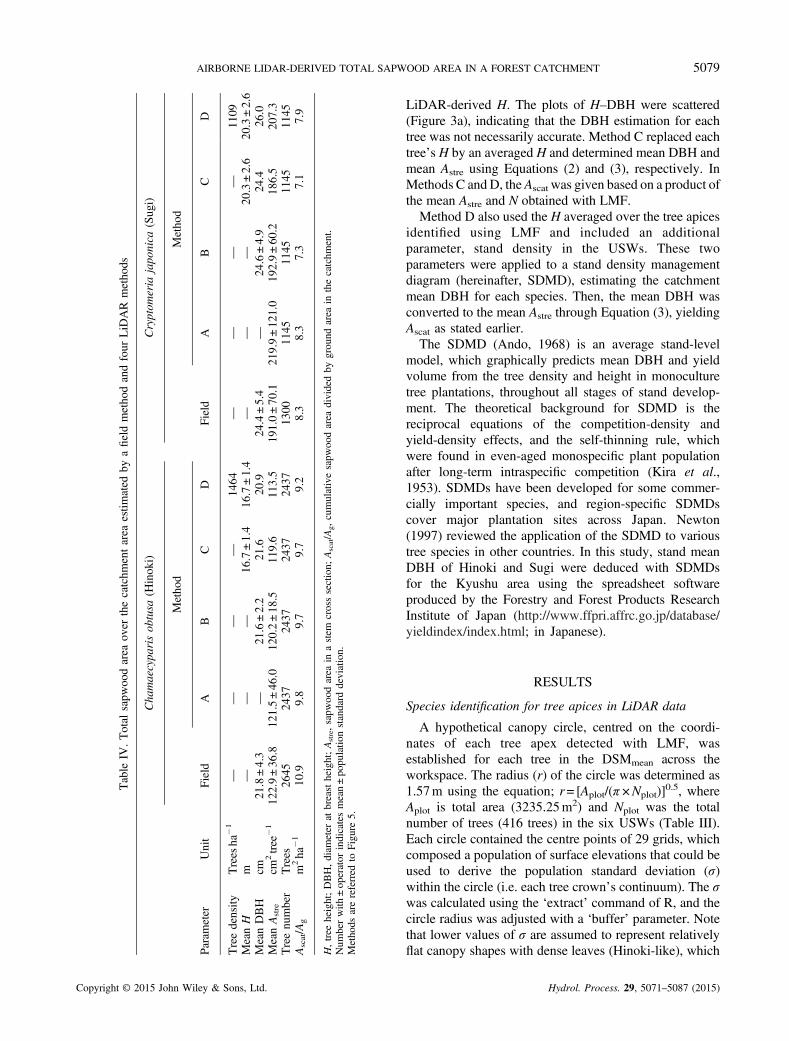
Table

IV.Total

sapw

oodarea

over

thecatchm

entarea

estim

ated

byafieldmethodandfour

LiDAR

methods

Param

eter

Unit

Chamaecyparisobtusa

(Hinoki)

Cryptom

eria

japonica

(Sugi)

Field

Method

Field

Method

AB

CD

AB

CD

Treedensity

Treesha

�1

——

——

1464

——

——

1109

MeanH

m—

——

16.7±1.4

16.7±1.4

——

—20.3±2.6

20.3±2.6

MeanDBH

cm21.8±4.3

—21.6±2.2

21.6

20.9

24.4±5.4

—24.6±4.9

24.4

26.0

MeanAstre

cm2tree

�1

122.9±36.8

121.5±46.0

120.2±18.5

119.6

113.5

191.0±70.1

219.9±121.0

192.9±60.2

186.5

207.3

Treenumber

Trees

2645

2437

2437

2437

2437

1300

1145

1145

1145

1145

Ascat/A

gm

2ha

�1

10.9

9.8

9.7

9.7

9.2

8.3

8.3

7.3

7.1

7.9

H,tree

height;DBH,diam

eter

atbreastheight;Astre,sapw

oodarea

inastem

crosssection;

Ascat/A

g,cumulativesapw

oodarea

dividedby

ground

area

inthecatchm

ent.

Num

berwith

±operator

indicatesmean±populatio

nstandard

deviation.

Methods

arereferred

toFigure5.



LiDAR-derived H. The plots of H–DBH were scattered(Figure 3a), indicating that the DBH estimation for eachtree was not necessarily accurate. Method C replaced eachtree’s H by an averaged H and determined mean DBH andmean Astre using Equations (2) and (3), respectively. InMethods C and D, the Ascat was given based on a product ofthe mean Astre and N obtained with LMF.Method D also used the H averaged over the tree apices

identified using LMF and included an additionalparameter, stand density in the USWs. These twoparameters were applied to a stand density managementdiagram (hereinafter, SDMD), estimating the catchmentmean DBH for each species. Then, the mean DBH wasconverted to the mean Astre through Equation (3), yieldingAscat as stated earlier.The SDMD (Ando, 1968) is an average stand-level

model, which graphically predicts mean DBH and yieldvolume from the tree density and height in monoculturetree plantations, throughout all stages of stand develop-ment. The theoretical background for SDMD is thereciprocal equations of the competition-density andyield-density effects, and the self-thinning rule, whichwere found in even-aged monospecific plant populationafter long-term intraspecific competition (Kira et al.,1953). SDMDs have been developed for some commer-cially important species, and region-specific SDMDscover major plantation sites across Japan. Newton(1997) reviewed the application of the SDMD to varioustree species in other countries. In this study, stand meanDBH of Hinoki and Sugi were deduced with SDMDsfor the Kyushu area using the spreadsheet softwareproduced by the Forestry and Forest Products ResearchInstitute of Japan (http://www.ffpri.affrc.go.jp/database/yieldindex/index.html; in Japanese).

RESULTS

Species identification for tree apices in LiDAR data

A hypothetical canopy circle, centred on the coordi-nates of each tree apex detected with LMF, wasestablished for each tree in the DSMmean across theworkspace. The radius (r) of the circle was determined as1.57m using the equation; r= [Aplot/(π ×Nplot)]

0.5, whereAplot is total area (3235.25m2) and Nplot was the totalnumber of trees (416 trees) in the six USWs (Table III).Each circle contained the centre points of 29 grids, whichcomposed a population of surface elevations that could beused to derive the population standard deviation (σ)within the circle (i.e. each tree crown’s continuum). The σwas calculated using the ‘extract’ command of R, and thecircle radius was adjusted with a ‘buffer’ parameter. Notethat lower values of σ are assumed to represent relativelyflat canopy shapes with dense leaves (Hinoki-like), which

Hydrol. Process. 29, 5071–5087 (2015)

http://www.ffpri.affrc.go.jp/database/yieldindex/index.html

http://www.ffpri.affrc.go.jp/database/yieldindex/index.html

Figure 7. (a, b) Histograms for height of the tree apex (H), and (c, d) thoshypothetical canopy circle (1.57m in radius). Data were obtained from uniformin the digital surface model composed of the maximum (DSMmax) and mean (D

indicate threshold values for separating the spec

Figure 6. Digital surface model, which is composed of surface elevationgrids obtained from the maximum value of dispersed points falling in eachgrid (DSMmax). Right and left shaded areas indicate the uniform specieswindows (USWs) of Chamaecyparis obtusa (Hinoki) and Cryptomeriajaponica (Sugi), which are shown as h2 and s3 in Figure 1b, respectively.The points indicate local maxima detected with local maximum filtering



are continuous to neighbouring trees. Conversely, thehigher values of σ would represent relatively conicalcrown shapes with clumped leaves (Sugi-like), which areisolated from neighbouring trees. The data set for eachtree apex including the coordinates, H, and σ wereprepared across the entire area of the workspace. Next,the tree apices in the catchment or each USW wereextracted based on the coordinates of those areas in theDTM. Thus, grids outside the area beside the edges wereincluded for detecting tree apices using LMF and forcalculating σ in the canopy circle. Figure 6 showed thatthe LiDAR-derived local maxima succeeded in identify-ing the tops of mounds in DSMmax (i.e. tree apices).Figure 7 shows the frequency distributions of the H and

σ for each species in the USWs, revealing a noveldistinction between Hinoki and Sugi crown characteris-tics. All the tree apices in the three USWs of each specieswere aggregated, and threshold values were obtainedfrom the mean± three sample standard deviations of Hand σ (Table III). We noted that trees with H>19.7m

e for the population standard deviation (σ) of 29 levels of grids within aspecies windows for Hinoki (a, c) and Sugi (b, d). H and σ were obtainedSMmean) pulse level in each grid, respectively. Vertical dots with numbers

ies (mean ± three sample standard deviations)

Hydrol. Process. 29, 5071–5087 (2015)


could be classified as Sugi trees in the USWs. An overlapwas observed between Hinoki and Sugi in H>14.4m.However, we also noted that all trees with H>14.4m andσ>1.3m could be classified as Sugi. Any other trees thatdid not meet these criteria could be classified as Hinokitrees. In addition, some tree apices (28.3% of total) in theUSWs of Sugi were in the class of Hinoki (i.e. H≤ 19.7mand σ ≤1.3m).Combination of the LMF technique and the criteria for

species detection allowed us to create a map fordistribution of all ‘estimated’ Hinoki and Sugi tree apicesin the YEC (Figure 8). A total of 3582 tree apices wereidentified; in other words, 90.8% of 3945 field-verified‘actual’ trees were identified using LMF. The numbers ofthe LiDAR-identified Hinoki and Sugi were 2437 and1145, respectively (Table IV), which represented 92.1%and 88.1% of their actual populations. Note that thedistribution of the species was consistent with traditionalforestry guidelines (i.e. planting Hinoki trees on themiddle of the slope and Sugi trees in the valley).

LiDAR-derived total sapwood area overthe catchment area

Figure 9a and b shows the frequencies of LiDAR-derived H in the catchment. Using the LiDAR-derived H,Equation (2) allowed us to calculate the LiDAR-derivedDBH. Figure 9c and d shows that the LiDAR estimationcaptured canonical forms of the field-derived distributions.

Figure 8. Distribution of the estimated Chamaecyparis obtusa (Hinoki) and Cdetected using local maximum filtering on the digital surface model compose

into the two species based on th


LiDAR-derived and field-derived mean DBHs (Table IV)were not statistically different (P=0.12 and 0.31 in Hinokiand Sugi, respectively; Welch’s t-test). Departures inFigure 9c and d are the result of steeper tails on the left andright sides of the probability density function, resulting inthe DBH distribution having negative kurtosis in bothspecies. In Sugi, the tail on the left side of the function isflatter than the right side, resulting in negative skewness ofthe distribution.The LiDAR-derived Ascat/Ag obtained from Methods

A–D were compared with Ascat/Ag obtained from the fieldsurvey method (Table IV and Figure 10). In MethodsA–C, the LiDAR-derived Ascat/Ag of Hinoki was almost0.9, while that of Sugi ranged from 0.85 to 1.00 relative tothe field-derived value. In Method D, the numbers were0.84 for Hinoki and 0.95 for Sugi. The results indicatethat Method D is able to reproduce the actual Ascat/Ag withan accuracy that was comparable with the other LiDARmethods.

DISCUSSION

Kumagai et al. (2008, 2014) reported that the differencein ET among several sample plots in the same catchmentwas mainly determined by the variation in Ascat/Ag, whichwas affected by the slope position of each plot. Thescaling step from the stand-level total sapwood area overground area to catchment-level Ascat/Ag includes a

ryptomeria japonica (Sugi) tree apices in the catchment. Tree apices wered of the maximum pulse level in each grid. All tree apices were separatede criteria offered in this study

Hydrol. Process. 29, 5071–5087 (2015)

Figure 9. Histograms for LiDAR-derived height of tree apices for (a) Hinoki and (b) Sugi in the catchment. Probability density of diameter at breastheight (DBH) estimated from LiDAR-derived H is compared with field-derived DBH for (c) Hinoki and (d) Sugi. Vertical lines and dots indicted

mean values

Figure 10. LiDAR-derived cumulative sapwood area divided by ground area (Ascat/Ag) in (a) Hinoki and (b) Sugi. Field-derived Ascat/Ag (Field) was usedas a reference value for the other Ascat/Ag estimated with Methods A–D. Table IV presents values of Ascat/Ag


Copyright © 2015 John Wiley & Sons, Ltd. Hydrol. Process. 29, 5071–5087 (2015)


considerable amount of variation in stand density andsapwood area (e.g. Ford et al., 2007), and a field samplingcampaign is inevitably limited in terms of the areacovered by the tree census.Here, our estimation of Ascat with LiDAR was less

influenced by slope position of the sample plots than thathas been reported in other studies based on field surveys.Tree apices were identified evenly across the catchmentarea, and the windows for extracting species-specificcharacteristics of the canopy (i.e. USWs) can beestablished on slopes with various angles and aspectsusing GIS (Table III). Moreover, laser scanning from anairborne platform requires only a short time; for example,it took 1hour to survey the entire area of the YECincluding the nearby surrounding area. Thus, the LiDARtechnology can be effective in monitoring Ascat/Ag in acatchment of more than several hectares especially inmountainous areas. Moreover, the LiDAR enablesmonitoring Ascat/Ag repeatedly, such as for planning thethinning and confirming the results throughout all stagesof stand development.

Variations in DBH versus Astre relationship

Spatial variation in the DBH–Astre relationships withinthe catchment should not be a source of error in the Ascat/Ag estimate. Practically, the use of the DBH–Astre

relationship (Figure 4) is essential for estimating notonly field-derived Ascat/Ag but also the values obtained inMethods B–D. In reality, the DBH–Astre relationshipsvaried between the partial plots in the same catchment,mainly because of their slope positions (Kumagai et al.,2007). However, we minimized the variation inDBH–Astre relationships among slope positions byconducting data collection across the entire area of thecatchment.We should choose an adequate DBH–Astre relationship

according to the location of study site in Hinoki or theconditions for sapflow measurement in Sugi. In Figure 4,DBH–Astre relationships in the YEC were applied to thosein the Miyazaki Experimental Forest in Kumagai et al.(2005b) for each species. Although data were obtainedwhen the two plantations were of similar ages (42 and51 years old in YEC and Miyazaki Experimental Forest,respectively), there was some degree of differencebetween the two studies. The difference in Hinoki couldbe induced by the variety of the subject tree speciesand/or site conditions. Sampling in Kumagai et al.(2005b) was conducted in the central mountain range(1150ma.s.l.) on Kyushu Island where annual precipita-tion (3500mm) was larger than in the YEC. We notedthat that the curve of this study can be applied to Hinokiplantations around the headwaters of the Onga River innorthern Kyushu area.


On the other hand, the difference in Sugi was caused bythe difference in the estimating procedure for Astre. Theintermediate wood (i.e. white band) was not included inAstre in this study, while Kumagai et al. (2005b) included it.If the intermediate part is involved in determining Astre, thecurve of the DBH–Astre relationship in the YEC is identicalto that of Kumagai et al. (2005b). Thus, we should choosethe relationship of Sugi based on the location of the sensorprobes for measuring sapflow rate. In summary, one shouldapply the relationship of Kumagai et al. (2005b) if sensorprobes are placed across the depth of sapwood and theintermediate wood. On the other hand, the relationshipobtained in this study should be used if the sensor probeswere placed only across the SWD.

Errors in LiDAR-derived values to estimate Ascat/Ag

The LiDAR-derived H appears to be reliable in thisstudy. Some previous studies suggested that insufficientlaser pulse density was likely to cause underestimations ofH and N because of higher probability of failure to hit thetree apices (Persson et al., 2002; Gaveau and Hill, 2003).However, LiDAR-derivedH had an accuracy of better than1m in Hinoki (Hirata et al., 2009), and even in a Sugiplantation with a mean slope angle of approximately 38°(Takahashi et al., 2005). The present study carried outLiDAR data processes similar to that in the two previousstudies. The grid size (0.5m) in this study was somewhatlarger than that in the previous two studies (0.25–0.33m),resulting in a small number of interpolations of blank gridsin DSMs. Laser pulse density (30 pointsm�2) was higherthan that of Takahashi et al. (2005) (8.80–15.60pointsm�2) and somewhat smaller than that of Hirataet al. (2009) (40.5 pointsm�2), indicating high probabilityof tree apices hit by the laser pulses.However, underestimation of N seemed to lead to

underestimations of Ascat/Ag in the four LiDAR methods.LiDAR-derived N were 0.92 and 0.88 of the true numberin Hinoki and Sugi, respectively (Table IV), whichindicates omission errors of approximately 9% averagedacross the two species. Takahashi et al. (2005) showedthat some small trees were not detected if the height andcrown radius were smaller than the mean values of thesites. In principle, such errors in terms of omitting treeapices could occur in any LiDAR scans of a forest with acertain tree density, and the YEC was no exception.The mutual error in the species identification might not

significantly influence the estimation of Ascat/Ag for eachspecies. Separating tree apices into the two species wasreasonably accurate. Local maxima after the speciesseparation were plotted on the orthophoto of thecatchment, which allowed us to check the consistencyof the estimated species to actual species. Errors inspecies identification were 436 trees (17.9%) and 197

Hydrol. Process. 29, 5071–5087 (2015)


trees (17.2%) in the estimated Hinoki and Sugipopulations, respectively. As described earlier, theomission errors occurred at a similar rate in the twopopulations (Table IV), and the mean value of LiDAR-derived DBH was comparable with that of field-derivedDBH (Figure 9c and d). These results suggest that a largenumber of small Sugi trees were assigned as Hinoki,while a small number of large Hinoki trees weredetermined to be Sugi. However, >82% of all tree apicesrepresented the correct species; thus, the difference in treesize composition between the field-derived and LiDAR-derived populations might have a minor effect on theAscat/Ag estimates for each species. Our threshold valuesin the criteria may not be universally applied to otherplantations, because the H and σ are sensitive to stand ageand site quality. However, our approach, which includedmaking examination windows (i.e. USWs) inside theDSMs, can generally be applied to other plantations,where parts of the area are composed of homogeneousspecies.

Field campaigns required for estimating Ascat/Ag in LiDARmethods

Method A is the most simple and accurate but does notmake the best use of remote-sensing LiDAR technology.The LiDAR-derived H was directly converted to eachtree’s Astre in Method A. Resultant Ascat/Ag seemed toprovide the best estimate of the field-derived Ascat/Ag

among the four LiDAR methods. However, obtaining theH–Astre relationship (Figure 3b) again requires labour-intensive field campaigns for every site. For example, 47and 27 points of Hinoki and Sugi, respectively (Fig-ure 3b), required 296 increment borer samples in total.Such a large number of stem injuries is not acceptable innormal commercial plantations.Method B and C also required considerable measure-

ments in field. Conversion from LiDAR-derived H toDBH is a necessary first step for estimating Ascat. The H–DBH plots had many scattered points (Figure 3a), andthus, the derived Equation (2) did not have a very highprediction capability. The value gained through increas-ing the number of samples would not justify the increasedcosts of field observations. In this study, LiDAR-derivedmean DBH was almost consistent with field-derived meanDBH in both species (Figure 9c and d), so that Equation(2) may not be a major source of error. Nevertheless, thisconsistency would not be expected in other sites whereintensive field surveys cannot be conducted. Obviously,Methods A–C require extensive field campaigns toprepare either an ‘ad hoc’ DBH–Astre or DBH–Hrelationship for the objective site. Thus, Method A–Ccannot be used as standard, minimal labour procedure, fordeducing Ascat/Ag at other sites.


Applying SDMD to estimate Ascat/Ag

Method D reproduced the field-derived Ascat reasonablywell (Table IV). Note that only LiDAR-derived H and N,and the ‘ready-made’ SDMD with a DBH-Astre curve arerequired for estimating Ascat under Method D. TheLiDAR-derived tree density and mean H in a catchmentcan be used to parameterize average stand-level models inSDMD with no scale gaps. Moreover, LiDAR can detectthe tree apices across more than several hectares; clearly,collecting this type of data through field observation is notpractical. In this sense, Method D is the most appropriateamong the four methods offered here.The robustness of Ascat/Ag estimation with Method D

was elucidated through a sensitivity analysis (Figure 11a).As mentioned earlier, LiDAR-derived N inevitablyunderestimate the true N, which will be a major sourceof error in LiDAR-derived Ascat/Ag. Changing Ascat/Ag

was examined through the manipulation of N under afixed mean tree height (16.7m and 20.3m in Hinoki andSugi, respectively). Where LiDAR-derived N equaled thefield-derived N (i.e. relative N=1.0), the relative Ascat/Ag

was predicted to be 0.87 in Hinoki and 1.00 in Sugi. TheSugi case is an ideal example for showing the robustnessof Ascat/Ag estimation when Method D is used inuninvestigated plantations. We should be able to realizeless than 8% underestimation of Ascat/Ag within the rangeof 0–20% reduction in LiDAR-derived N relative toactual values. In the case of Hinoki, the Ascat/Ag wasunderestimated even at a relative N=1.0, because theSDMD somewhat underestimates DBH in the YEC.However, underestimation of Ascat/Ag was less than 20%within the range of 0–20% reduction in N. AlthoughSDMDs will not necessarily predict the actual DBH insome plantations, the errors never diminish the potentialusage of the diagrams. SDMDs are able to predict stand-average DBH of the plantations where the investigatorcannot conduct field surveys.The reduction in relative Ascat/Ag is gradual in

comparison with the reduction in relative N (Figure 11a),resulting from a certain amount of compensation by meanDBH intensified with decreasing N (Figure 11b). In Sugi,the mean DBH (hence, mean Astre) was overestimated inthe process of Method D, but the intrinsic underestima-tion of N compensates the mean Astre overestimation,resulting in reasonable reproduction of Ascat/Ag

(Figure 10). The same compensation occurred in Hinoki,although Ascat/Ag was underestimated to a greater extentbecause SDMD underestimated mean DBH in the YEC.The estimates of mean DBH increase with decreasing Nin a given stand area in SDMD (Figure 11b). One of theprinciples of SDMD is the natural law of competition-density effect (Kira et al., 1953), which is expressed by

Hydrol. Process. 29, 5071–5087 (2015)

Figure 11. Sensitivity analysis of (a) LiDAR-derived cumulative sapwoodarea divided by ground area (Ascat/Ag) and (b) LiDAR-derived meandiameter at breast height (DBH). The LiDAR-derived tree number (N) ismanipulated under a fixed mean tree height (16.7 and 20.3m in Hinokiand Sugi, respectively). The LiDAR-derived Ascat/Ag and the mean DBHwere calculated with Method D. The values were relative to thecorresponding field-derived values. Arrows indicate the relative Ascat/Ag

or the relative mean DBH at underestimated N (0.92 and 0.88 in Hinokiand Sugi, respectively) estimated by the LiDAR technique in the

catchment


using the equation as 1/w=Aρ+B, where w is meanbiomass per plant, ρ is the number of plants per unit area,and A and B are constants. The reciprocal relationshipcan be also applied to the relationships between standdensity and basal area (hence, DBH) in conifer planta-tions (Ando, 1968).At a landscape level, the measure of Ascat/Ag might be

influenced by the site quality including atmospheric


factors such as solar radiation and atmospheric evapora-tive demand. The Ascat/Ag is closely related to Ecat

(Equation [1]), which is an important component of forestevapotranspiration (ET). The measured annual ET hasbeen reported to be conservative at each site (e.g. Roberts,1983; Kosugi and Katsuyama, 2007), and annual ET inthe 43 catchments across Japan had a linear relationshipwith mean annual air temperature (Komatsu et al., 2008).We can recommend use of the more efficient Method D

to estimate Ascat/Ag, because the accuracy was at a levelsimilar to the labour-intensive Methods A–C. The degreeof variation in the Ascat/Ag estimate between the fieldmethod and the LiDAR methods (Figure 10) wascomparable with the degree of variation in Js estimatesin a catchment (approximately ±10%; Kume et al., 2009;Kumagai et al., 2014). To estimate Ecat with greatestaccuracy, we have to consider not only how Js wasmeasured but also consider how the Ascat/Ag wasestimated considering the available funds for suchestimations. Use of airborne LiDAR with existingSDMDs is a less labour-intensive method for evaluatingAscat/Ag. Future work could also couple LiDAR measure-ments to quantify Ecat with field-based measurements ofprecipitation partitioning (i.e. throughfall, stemflow andinterception; Saito et al., 2013) from representative treespecies. The effects of species-specific canopy structureon the partitioning (such as Levia et al., 2015) could beused with LiDAR measurements of canopy structure on acatchment scale, to develop a more complete understand-ing of the hydrologic cycle of these plantations.

CONCLUSION

Four methods were examined for estimating Ascat usingLiDAR-derived data. Hinoki and Sugi were identifiedreasonably well employing the criteria of tree height andcanopy roughness in the USWs. The field-derived H–Astre

and H–DBH relationships were scattered despite intensivefield campaigns. The LiDAR technique underestimated N,which caused underestimation of Ascat/Ag. When SDMDsare used for estimating Ascat/Ag of uninvestigated forests,we should be able to realize less than 8% underestimationof Ascat/Ag within the range of 0–20% reduction in Nrelative to actual values. We suggest that couplingLiDAR-derived H and N with SDMDs requires the leastamount of labour and provides an effective method forestimating Ascat/Ag.

ACKNOWLEDGEMENTS

This study was conducted primarily under the project‘Development of innovative technologies for increasingin watershed runoff and improving river environment by

Hydrol. Process. 29, 5071–5087 (2015)


the management practice of devastated forest plantation’funded by Core Research for Evolutional Science andTechnology (CREST) of the Japan Science and Technol-ogy (JST). We are grateful to Drs Y. Onda, H. Kato, K.Nanko, A. Hirata, Y. Komatsu, T. Kasahara, N.Kobayashi, S. Hamada, T. Nonoda, D. F. Levia and T.Gomi for their support of field measurements and criticaladvice. TS and TK were supported by a grant from theJapanese Ministry of Agriculture, Forestry and Fisheries.

ABBREVIATIONS

Ascat/Ag

Copyright ©
2
Cumulative sapwood area over the catchmentarea (m2ha�1)

Astre
Sapwood area of a single tree in a stem crosssection (m2)
BRD,LBRD

Bark depth in the stem cross section (cm)

DBH, D
Diameter at breast height (cm; at approxi-mately 1.2m)
DTM
Digital terrain map DSMmax Digital surface map composed of the grids
with the maximum elevation among the firstreturns of the laser pulse fallen in each grid

DSMmean
Digital surface map composed of the gridswith mean elevation among the first returnsof the laser pulse fallen in each grid
Ecat
Transpiration rate in the catchment (mmd�1) Field Field-derived Ascat/Ag
GIS
Geographic information system H Individual tree height (m) Js Sap flux density (m3m�2 d�1) LiDAR Light detection and ranging LMF Local maximum filtering N The number of trees σ Population standard deviation of the height of
29 grids in the hypothetical canopy circle inDSMmean

SDMD
Stand density management diagram SWD,LSWD
Sapwood depth in the stem cross section (cm)

USW
Uniform species window YEC Yayama experimental catchment
REFERENCES

Alsheimer M, Köstner B, Falge E, Tenhunen JD. 1998. Temporal andspatial variation in transpiration of Norway spruce stands within aforested catchment of the Fichtelgebirge, Germany. Annals of ForestScience 55: 103–123.

015 John Wiley & Sons, Ltd.

Ando T. 1968. Ecological studies on the stand density control in even-aged pure stand. Bulletin of the Government Forest Experiment Station(Tokyo) 210: 1–153. (in Japanese with English summery)

Ford CR, Hubbard RM, Kloeppel BD, Vose JM. 2007. A comparison ofsap flux-based evapotranspiration estimates with catchment-scale waterbalance. Agricultural and Forest Meteorology 145: 176–185.

Gaveau DLA, Hill RA. 2003. Quantifying canopy height underestimationby laser pulse penetration in small-footprint airborne laser scanningdata. Canadian Journal of Remote Sensing 29(5): 650–657.

GRASS Development Team. 2012. Geographic resources analysis supportsystem (GRASS) software. Open Source Geospatial FoundationProject. http://grass.osgeo.org [Accessed February 18, 2014].

Hirata Y, Furuya N, Suzuki M, Yamamoto H. 2009. Airborne laserscanning in forest management: individual tree identification and laserpulse penetration in a stand with different levels of thinning. ForestEcology and Management 258: 752–760.

Hyyppä J, Lehikoinen M, Inkinen M. 2001. A segmentation-based methodto retrieve stem volume estimates from 3-D tree height modelsproduced by laser scanners. IEEE Transactions on Geoscience andRemote Sensing 39(5): 969–975.

Inoue Y, Miyahara H. 1954. On the yield-table of Sugi stand at KasuyaUniversity Forest. Reports of the Kyushu University Forests 2: 15–50.(in Japanese)

Japan Forest Agency. 1957. Yield table of Hinoki stands in Kyushu-area.The Ministry of Agriculture, Forestry and Fisheries of Japan, Tokyo. (inJapanese)

Japan Forest Agency. 2013. Annual report on forest and forestry in Japan:fiscal year 2013. The Ministry of Agriculture, Forestry and Fisheries ofJapan, Tokyo, pp. 85. (in Japanese)

Kawana A. 1992. Forestation in Forestry, 3rd edn. Asakura: Tokyo, pp.101. (in Japanese)

Kira T, Ogawa H, Sakazaki N. 1953. Intraspecific competition amonghigher plants. I. Competition-density-yield interrelationship in regularlydispersed population. Journal of the Institute of Polytechnics (OsakaCity University) Series 4: 1–16.

Komatsu H, Maita E, Otsuki K. 2008. A model to estimate annual forestevapotranspiration in Japan from mean annual temperature. Journal ofHydrology 348: 330–340.

Kosugi Y, Katsuyama M. 2007. Evapotranspiration over a Japanesecypress forest. II. Comparison of the eddy covariance and water budgetmethods. Journal of Hydrology 334: 305–311.

Kumagai T, Aoki S, Nagasawa H, Mabuchi T, Kubota K, Inoue S, UtsumiY, Otsuki K. 2005a. Effects of tree-to-tree and radial variations on sapflow estimates of transpiration in Japanese cedar. Agricultural andForest Meteorology 135: 110–116.

Kumagai T, Nagasawa H, Mabuchi T, Ohsaki S, Kubota K, Kogi K,Utsumi Y, Koga S, Otsuki K. 2005b. Sources of error in estimatingstand transpiration using allometric relationships between stem diameterand sapwood area for Cryptomeria japonica and Chamaecyparisobtusa. Forest Ecology and Management 206: 191–195.

Kumagai T, Aoki S, Shimizu T, Otsuki K. 2007. Sap flow estimates ofstand transpiration at two slope positions in a Japanese cedar forestwatershed. Tree Physiology 27: 161–168.

Kumagai T, Tateishi M, Shimizu T, Otsuki K. 2008. Transpiration andcanopy conductance at two slope positions in a Japanese cedar forestwatershed. Agricultural and Forest Meteorology 148: 1444–1455.

Kumagai T, Tateishi M,Miyazawa Y, Kobayashi M, Yoshifuji N, KomatsuH, Shimizu T. 2014. Estimation of annual forest evapotranspiration froma coniferous plantation watershed in Japan (1): water use components inJapanese cedar stands. Journal of Hydrology 508: 66–76.

Kume A, Tsuruta K, Komatsu H, Kumagai T, Higashi N, Shinohara Y,Otsuki K. 2009. Effects of sample size on sap flux-based stand-scaletranspiration estimates. Tree Physiology 30: 129–138.

Kuroda K, Yamashita K, Fujiwara T. 2009. Cellular level observation ofwater loss and the refilling of tracheids in the xylem of Cryptomeriajaponica during heartwood formation. Trees 23: 1163–1172.

Lefsky MA, Cohen WB, Parker GG, Harding D. 2002. Lidar remotesensing for ecosystem studies. BioScience 52(1): 19–30.

Levia DF, Näthe MK, Bischoff S, Richter S, Legates DR. 2015.Differential stemflow yield from European beech saplings: the role ofindividual canopy structure metrics. Hydrological Processes 29: 43–51.

Hydrol. Process. 29, 5071–5087 (2015)

http://grass.osgeo.org


Nagai S, Taniguchi Y. 2001. Air permeability in wood of Cryptomeriajaponica D. Don: air permeability in heartwood, white zone wood andsapwood in green logs. Zairyo 50: 409–414. (in Japanese with Englishsummary)

Nagai S, Utsumi Y. 2012. The function of intercellular spaces along theray parenchyma in sapwood, intermediate wood, and heartwood ofCryptomeria japonica (Cupressaceae). American Journal of Botany 99:1553–1561.

Nagakura J, Shigenaga H, Akama A, Takahashi M. 2004. Growth andtranspiration of Japanese cedar (Cryptomeria japonica) and Hinokicypress (Chamaecyparis obtusa) seedlings in response to soil watercontent. Tree Physiology 24: 1203–1208.

Newton PF. 1997. Stand density management diagrams: review of theirdevelopment and utility in stand-level management planning. ForestEcology and Management 98: 251–265.

Nobuchi T, Harada H. 1983. Physiological features of the “white zone” ofsugi (Cryptomeria japonica D. Don) – cytological structure andmoisture content. Mokuzai Gakkaishi 29: 824–832.

Ohashi H, Motegi Y, Yasue M. 1985. Water distribution and wateralleyway in the living stem of Cryptomeria japonica. Research Bulletinof the Faculty College of Agriculture Gifu University 50: 111–129.

Pataki DE, Oren R. 2003. Species differences in stomatal control of waterloss at the canopy scale in a mature bottomland deciduous forest.Advances in Water Resources 26: 1267–1278.

Persson A, Holmgren J, Söderman U. 2002. Detecting and measuringindividual trees using an airborne laser scanner. PhotogrammetricEngineering and Remote Sensing 68: 925–932.

Popescu SC, Wynne RH, Nelson RF. 2002. Estimating plot-level treeheights with lidar: local filtering with a canopy-height based variablewindow size. Computers and Electronics in Agriculture 37: 71–95.

R Core Team. 2013. R: a language and environment for statisticalcomputing. R Foundation for Statistical Computing, Vienna, Austria.http://www.R-project.org/ [Accessed February 15, 2014].


Roberts J. 1983. Forest transpiration: a conservative hydrological process?Journal of Hydrology 66: 133–141.

Roberts S, Vertessy R, Grayson R. 2001. Transpiration from Eucalyptussieberi (L. Johnson) forests of different age. Forest Ecology andManagement 143: 153–161.

Roth BE, Slatton KC, Cohen MJ. 2007. On the potential for high-resolution lidar to improve rainfall interception estimates in forestecosystems. Frontiers in Ecology and the Environment 5: 421–428.

Saito T, Matsuda H, Komatsu M, Xiang Y, Takahashi A, Shinohara Y,Otsuki K. 2013. Forest canopy interception loss exceeds wet canopyevaporation in Japanese cypress (Hinoki) and Japanese cedar (Sugi)plantations. Journal of Hydrology 507: 287–299.

Takahashi T, Yamamoto K, Senda Y, Tsuzuku M. 2005. Estimatingindividual tree heights of sugi (Cryptomeria japonica D. Don)plantations in mountainous areas using small-footprint airborne LiDAR.Journal of Forest Research 10: 135–142.

Vierling KT, Vierling LA, Gould WA, Martinuzzi S, Clawges RM. 2008.Lidar: shedding new light on habitat characterization and modeling.Frontiers in Ecology and the Environment 6: 90–98.

Wilson KB, Hanson PJ, Mulholland PJ, Baldocchi DD, Wullschleger SD.2001. A comparison of methods for determining forest evapotranspi-ration and its components: sap-flow, soil water budget, eddy covarianceand catchment water balance. Agricultural and Forest Meteorology106: 153–168.

Wullschleger SD, Hanson PJ, Todd DE. 2001. Transpiration from a multi-species deciduous forest as estimated by xylem sap flow techniques.Forest Ecology and Management 143: 205–213.

Zimmermann R, Schulze E-D, Wirth C, Schulze E-E, McDonald KC,Vygodskaya NN, Ziegler W. 2000. Canopy transpiration in achronosequence of Central Siberian pine forests. Global ChangeBiology 6: 25–37.

Hydrol. Process. 29, 5071–5087 (2015)

http://www.R-project.org/

Documents

Using airborne LiDAR to determine total sapwood area …tomo-kumagai.eco.coocan.jp/hp1501.pdf · estimating stand transpiration in plantations ... remote sensing; ... Using airborne