Volumetric Attributes-Apparent Component and …mcee.ou.edu/aaspi/upload/AASPI_Consortium_Review...Volumetric Attributes-Apparent Component and Euler Curvature Attribute-Assisted Seismic

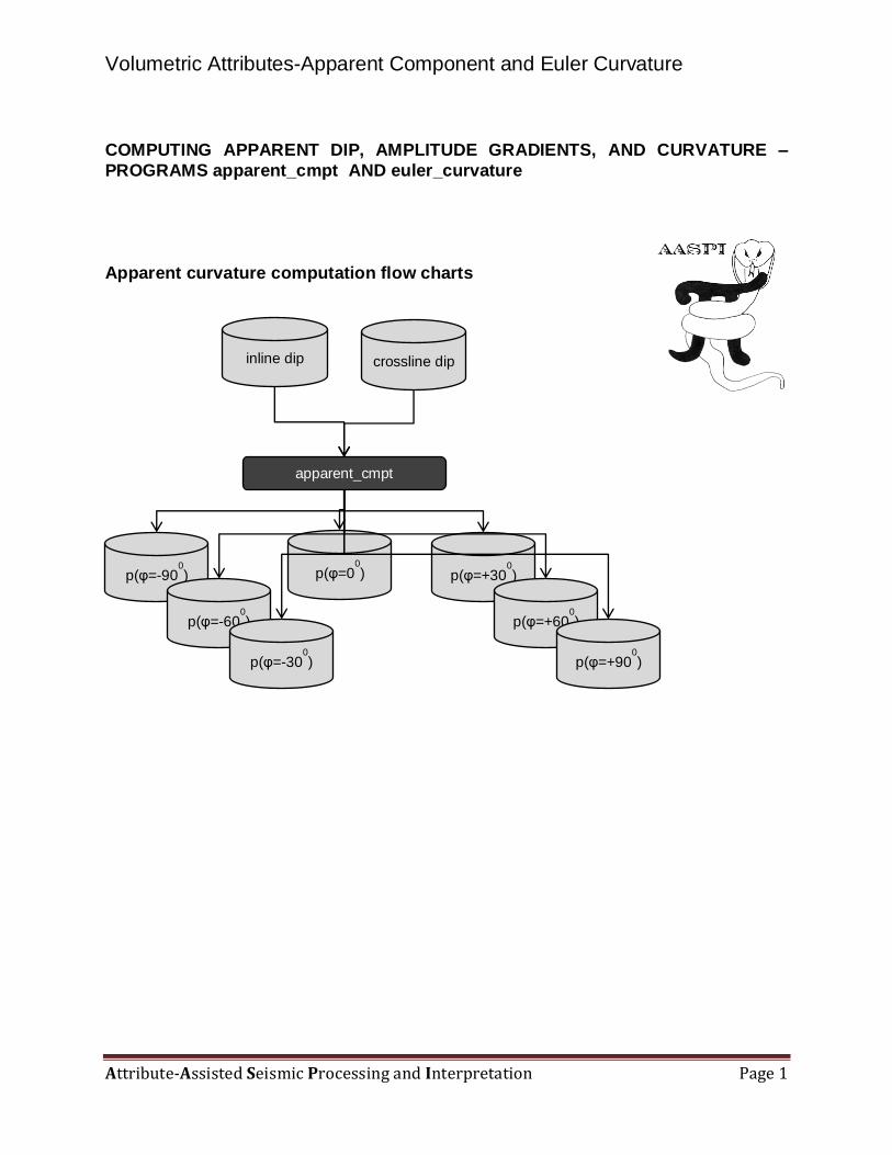
Volumetric Attributes-Apparent Component and Euler Curvature

Attribute-Assisted Seismic Processing and Interpretation Page 1

COMPUTING APPARENT DIP, AMPLITUDE GRADIENTS, AND CURVATURE –

PROGRAMS apparent_cmpt AND euler_curvature

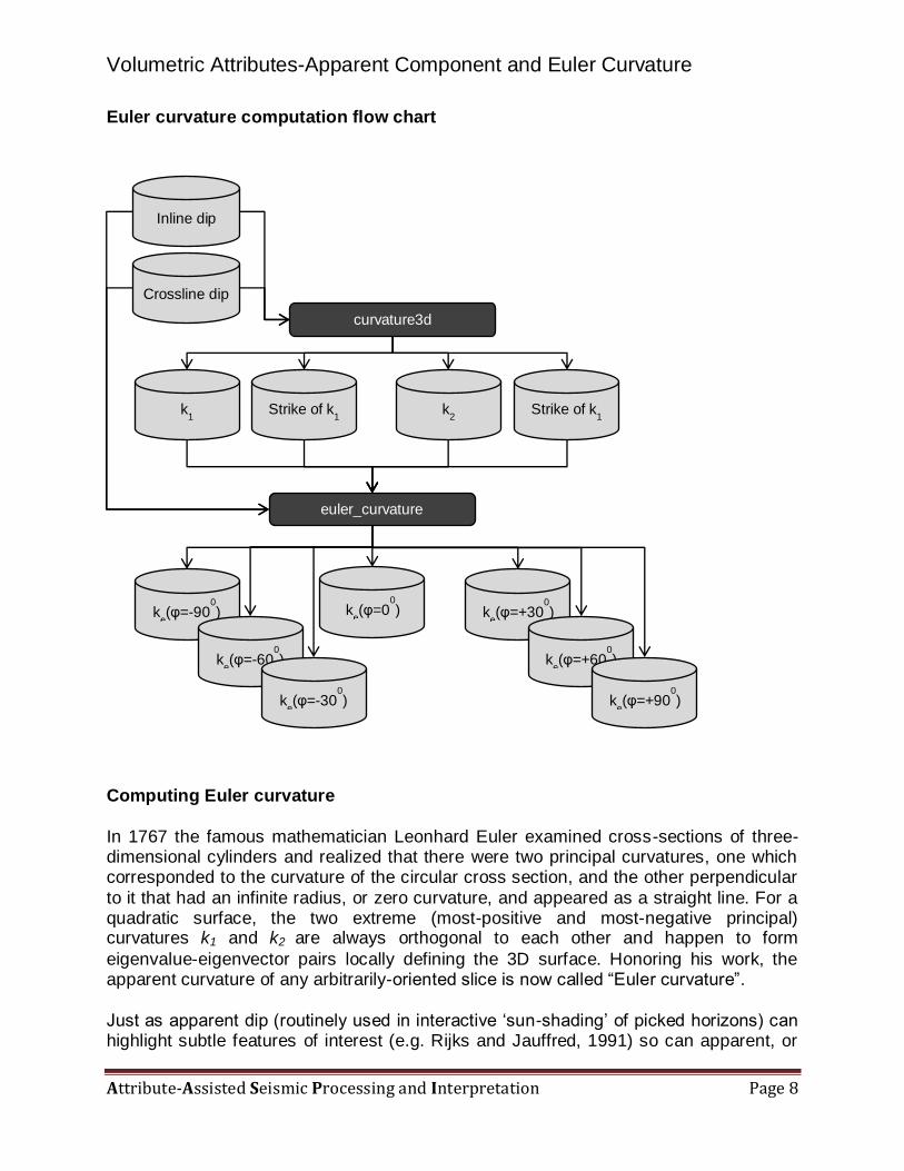
Apparent curvature computation flow charts

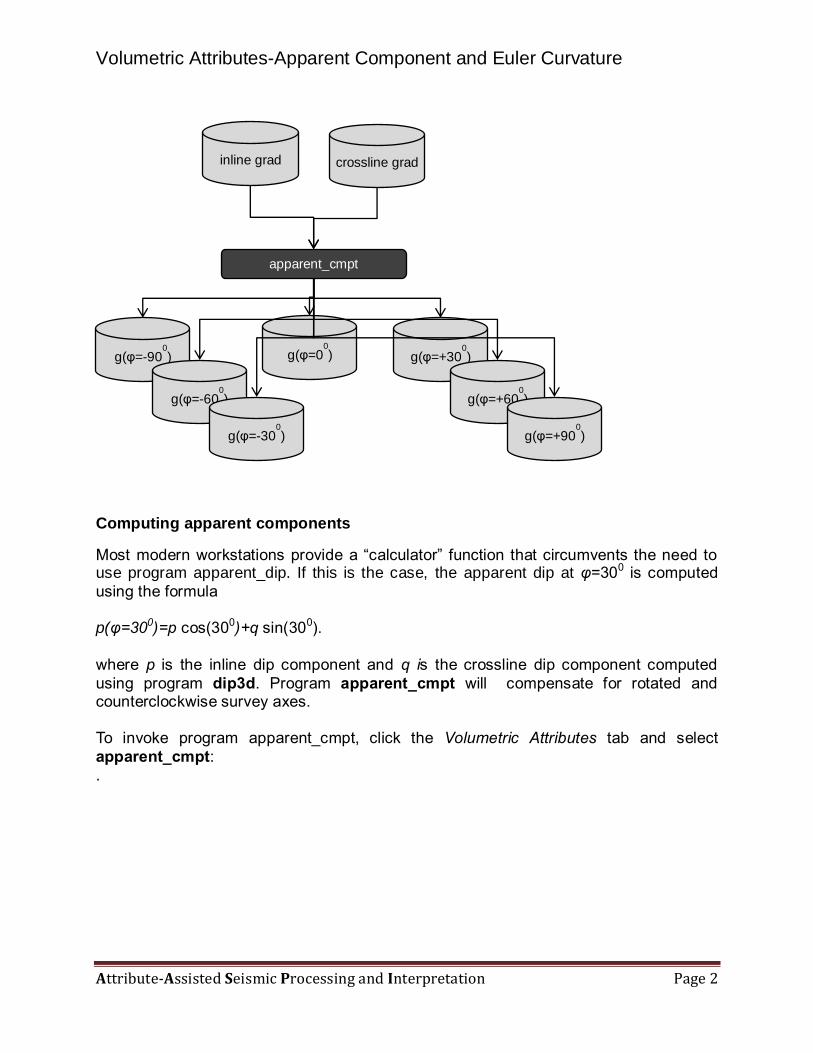
inline dip crossline dip

apparent_cmpt

p(φ=-900

)

p(φ=-600

)

p(φ=-300

)

p(φ=00

) p(φ=+300

)

p(φ=+600

)

p(φ=+900

)



Computing apparent components

Most modern workstations provide a “calculator” function that circumvents the need to use program apparent_dip. If this is the case, the apparent dip at φ=300 is computed

using the formula p(φ=300)=p cos(300)+q sin(300).

where p is the inline dip component and q is the crossline dip component computed

using program dip3d. Program apparent_cmpt will compensate for rotated and counterclockwise survey axes.

To invoke program apparent_cmpt, click the Volumetric Attributes tab and select

apparent_cmpt:

.

inline grad crossline grad

apparent_cmpt

g(φ=-900

)

g(φ=-600

)

g(φ=-300

)

g(φ=00

) g(φ=+300

)

g(φ=+600

)

g(φ=+900

)



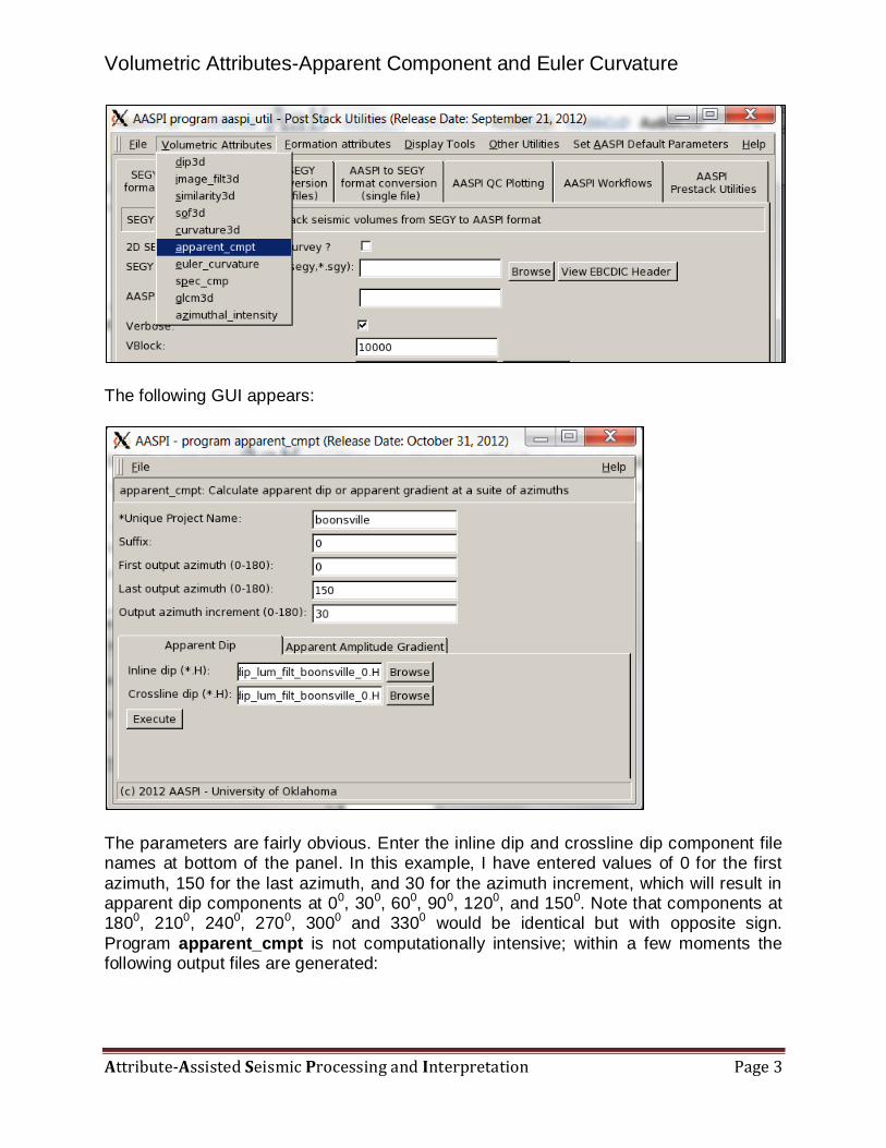
The following GUI appears:

The parameters are fairly obvious. Enter the inline dip and crossline dip component file names at bottom of the panel. In this example, I have entered values of 0 for the first

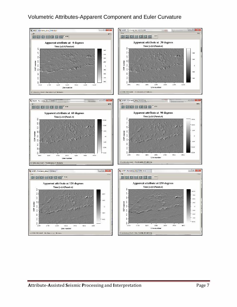
azimuth, 150 for the last azimuth, and 30 for the azimuth increment, which will result in apparent dip components at 00, 300, 600, 900, 1200, and 1500. Note that components at 1800, 2100, 2400, 2700, 3000 and 3300 would be identical but with opposite sign.

Program apparent_cmpt is not computationally intensive; within a few moments the following output files are generated:



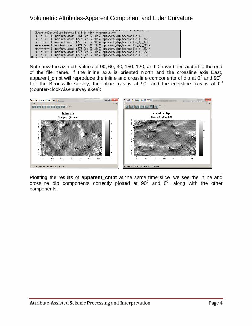
Note how the azimuth values of 90, 60, 30, 150, 120, and 0 have been added to the end of the file name. If the inline axis is oriented North and the crossline axis East,

apparent_cmpt will reproduce the inline and crossline components of dip at 00 and 900. For the Boonsville survey, the inline axis is at 900 and the crossline axis is at 00 (counter-clockwise survey axes):

Plottting the results of apparent_cmpt at the same time slice, we see the inline and

crossline dip components correctly plotted at 900 and 00, along with the other components.



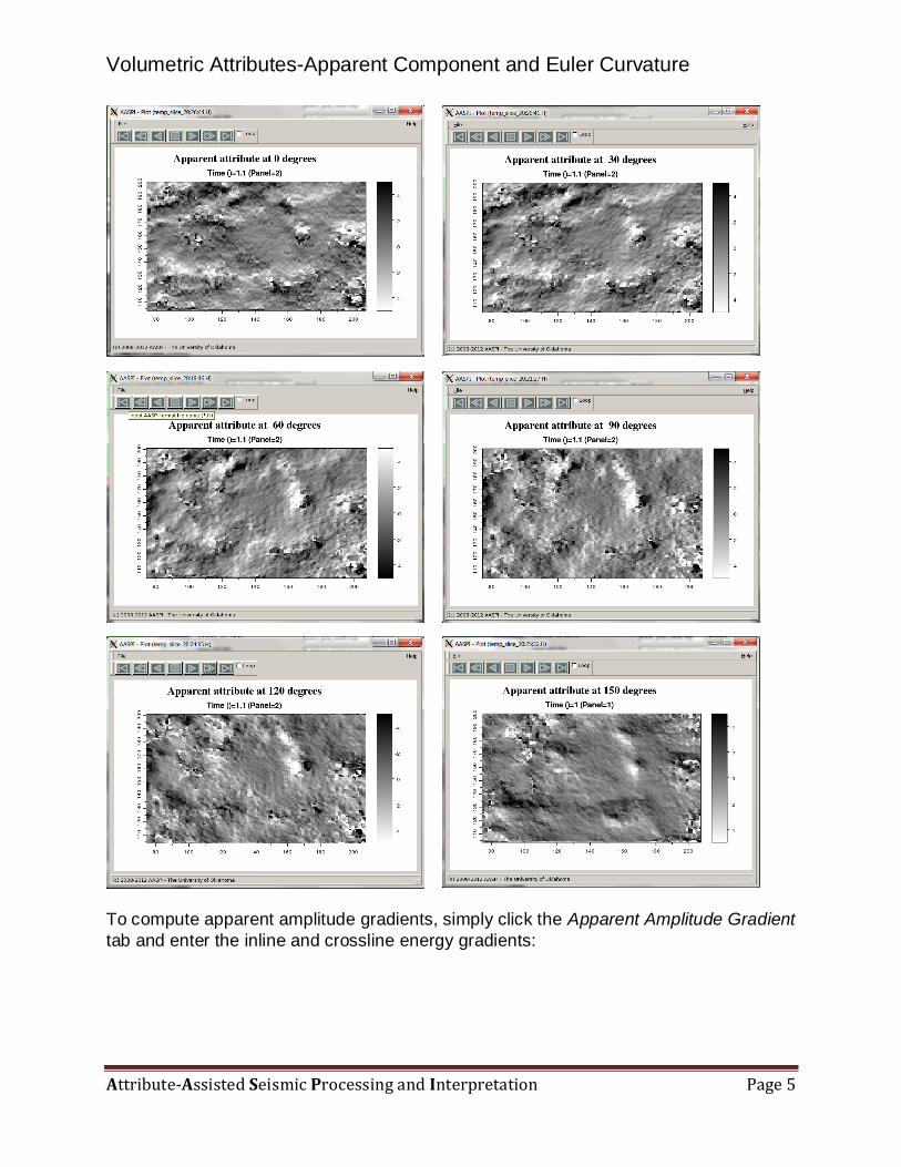
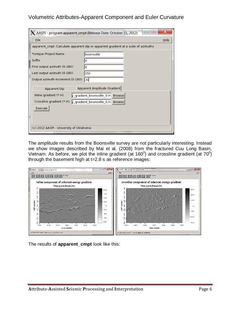
To compute apparent amplitude gradients, simply click the Apparent Amplitude Gradient

tab and enter the inline and crossline energy gradients:



The amplitude results from the Boonsville survey are not particularly interesting. Instead

we show images described by Mai et al. (2008) from the fractured Cuu Long Basin, Vietnam. As before, we plot the inline gradient (at 1600) and crossline gradient (at 700) through the basement high at t=2.8 s as reference images:

The results of apparent_cmpt look like this:





Euler curvature computation flow chart

Computing Euler curvature

In 1767 the famous mathematician Leonhard Euler examined cross-sections of three-dimensional cylinders and realized that there were two principal curvatures, one which corresponded to the curvature of the circular cross section, and the other perpendicular

to it that had an infinite radius, or zero curvature, and appeared as a straight line. For a quadratic surface, the two extreme (most-positive and most-negative principal) curvatures k1 and k2 are always orthogonal to each other and happen to form

eigenvalue-eigenvector pairs locally defining the 3D surface. Honoring his work, the apparent curvature of any arbitrarily-oriented slice is now called “Euler curvature”.

Just as apparent dip (routinely used in interactive ‘sun-shading’ of picked horizons) can highlight subtle features of interest (e.g. Rijks and Jauffred, 1991) so can apparent, or

Inline dip

Crossline dip

curvature3d

k1 Strike of k

1 k

2 Strike of k

1

euler_curvature

ke(φ=-90

0

)

ke(φ=-60

0

)

ke(φ=-30

0

)

ke(φ=0

0

) ke(φ=+30

0

)

ke(φ=+60

0

)

ke(φ=+90

0

)



Euler, curvature. The simplest way to envision Euler curvature is to envision a vertical slice striking at angle ψ from North through a fold. The intersection of the 3D fold with

the vertical slice results in a 2D curve. Now, at any point on that curve, find the 2D circle that is tangent to it. The reciprocal of the radius of this 2D circle is the value of the Euler curvature in thus vertical plane. Also note that one obtains the same circle whether

examining the plane from left to right or right to left. If (k1, ψ1) and (k2, ψ2) represent the magnitudes and strikes of the most-positive

and most-negative principal curvatures then the Euler curvature striking at an angle ψ’

in the dipping plane tangent to the analysis point (where the vectors corresponding to ψ’1 and ψ’2 are orthogonal) is given as

kψ’ = k1cos2(ψ’- ψ’2) + k2 sin2(ψ’- ψ’2).

Note the squares over the cosine and sine term, which mathematically gives the same value of Euler curvature whether we look in the +ψ’ or -ψ’ from the most-negative principal curvature strike direction, ψ’2. At this juncture the analogy to apparent dip (which would change sign) breaks down. While ψ’1 and ψ’2 will be perpendicular in the

dipping plane tangent to the surface, the strikes projected onto the horizontal x-y plane, ψ1 and ψ2 , will not in general be perpendicular to each other. For program euler_curvature, we define the value of ψ for the entire volume along the horizontal x-

y plane, project it onto to the dipping surface at each analysis point, apply equation 14.1, and compute k ψ’. The dip of the local surface is defined by the inline and crossline dip components p and q. The algorithm computes a suite of Euler curvatures

at azimuths ψ that are equally sampled in the x-y plane.

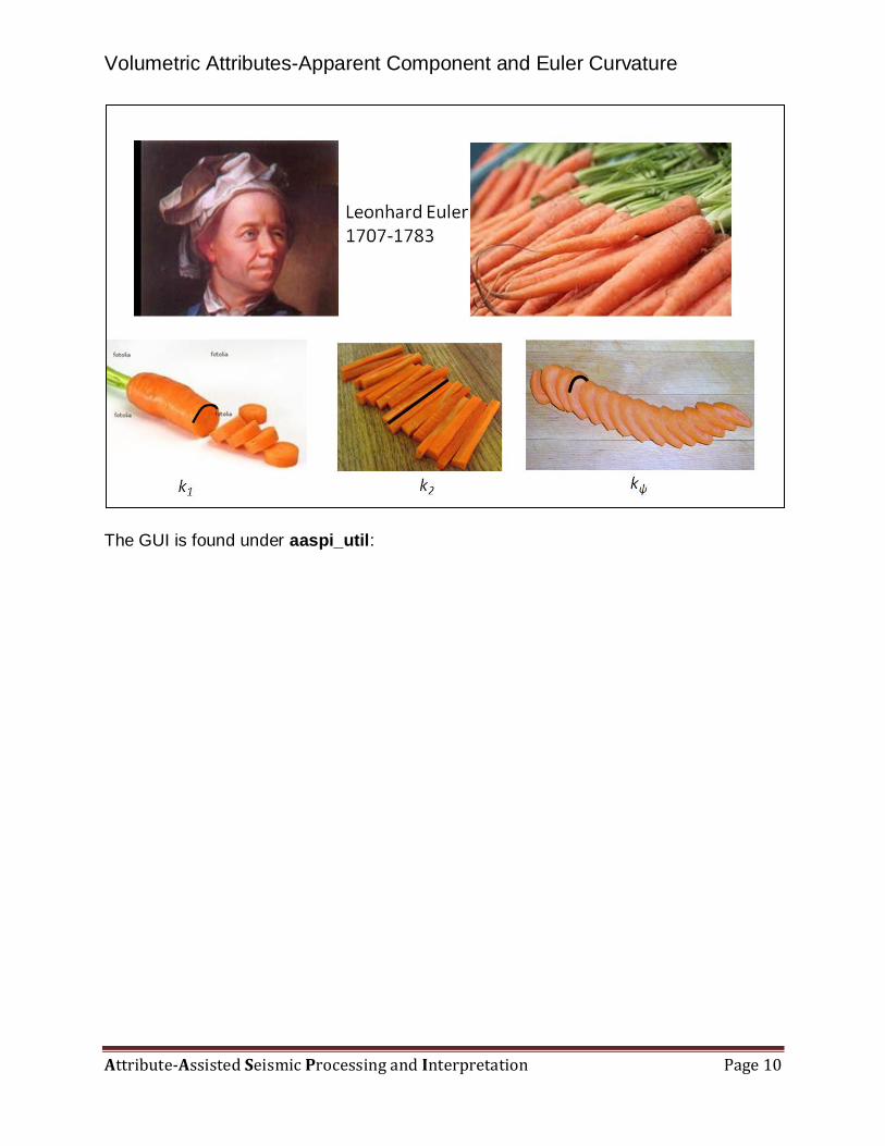
Tradition has it that Euler stumbled upon this formulation after his wife criticized him for

preparing the family soup - she was unsatisfied with both circular cut and julienned or longitudinal cuts. With his mathematical genius he was able to cut the carrots at any arbitrary manner:



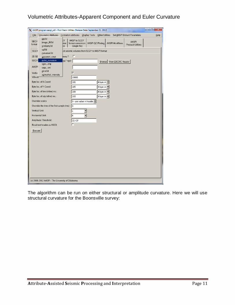
The GUI is found under aaspi_util:



The algorithm can be run on either structural or amplitude curvature. Here we will use structural curvature for the Boonsville survey:



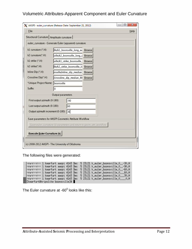
The following files were generated:

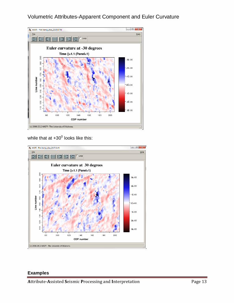
The Euler curvature at -600 looks like this:



while that at +300 looks like this:

Examples



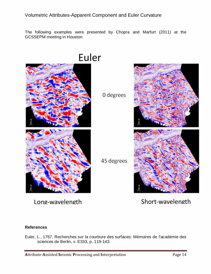
The following examples were presented by Chopra and Marfurt (2011) at the

GCSSEPM meeting in Houston:

References

Euler, L., 1767, Recherches sur la courbure des surfaces: Mémoires de l'académie des sciences de Berlin, v. E333, p. 119-143.

Long-wavelength Short-wavelength

Euler Curvature

http://math.dartmouth.edu/~euler/pages/E333.html

http://math.dartmouth.edu/~euler/pages/E333.html



Mai, H.T., K. J. Marfurt, and T. T. Mai, 2009, Multi-attributes display and rose diagrams for interpretation of seismic fracture lineaments, example from Cuu Long basin,

Vietnam: The 9th SEGJ International Symposium Imaging and Interpretation - Science and Technology for Sustainable Development, paper 1D93.

Documents

Volumetric Attributes-Apparent Component and …mcee.ou.edu/aaspi/upload/AASPI_Consortium_Review...Volumetric Attributes-Apparent Component and Euler Curvature Attribute-Assisted Seismic