Theme: J. Labour Markets and Migration

Paper Prepared for the Regional Studies Association European Conference

Diverse Regions: Buildung Resilient Communities and Territories

Izmir, Turkey, Monday 16th June – Wednesday 18 June 2014

A Three-Step Method for Delineating Functional Labour Market Regions

Dr. Per Kropp

Barbara Schwengler

D R A F T V E R S I O N

– The final paper will be published in a forthcoming issue of Regional Studies –

Dr. Per Kropp

IAB Saxony-Anhalt-Thuringia

Frau-v.-Selmnitz-Str. 6

D-06110 Halle

Germany

Mail: Per.Kropp@iab.de

Barbara Schwengler

Institute for Employment Research (IAB) of the Federal Employment Agency

Regensburger Str. 104

D-90478 Nuremberg

Germany

Mail: Barbara.Schwengler@iab.de

A Three-Step Method for Delineating Functional Labour Market Regions

Index

Abstract ...................................................................................................................................... 1

1 Introduction ......................................................................................................................... 3

2 Current state of research ..................................................................................................... 4

3 Data ..................................................................................................................................... 8

4 Method .............................................................................................................................. 11

5 Results ............................................................................................................................... 18

5.1 The cluster generator at work .................................................................................... 18

5.2 Choosing the analytically best delineation ................................................................ 19

5.3 Optimisation procedure ............................................................................................. 22

5.4 The robustness of the labour market delineation ....................................................... 25

5.5 Descriptive data ......................................................................................................... 27

5.6 Comparison with other delineations .......................................................................... 30

6 Conclusions and outlook ................................................................................................... 35

7 References ......................................................................................................................... 37

8 Endnotes ............................................................................................................................ 42

1

Abstract

In our paper we propose a new approach for delineating functional labour market regions

based on commuting flows with strong interactions within the region and few connections

with outside areas. As functional regions are an important basis for analysis in regional

science and for labour market and economic policy it is necessary to define functional regions

in an adequate way.

While previous studies devoted to the delineation of labour market regions have employed a

variety of methodological procedures, such as cluster analysis, the threshold method and

factor analysis, we apply the graph theoretical approach as a suitable method. Based on a

modification of a dominant flow approach we produce many meaningful delineations for

labour market regions using the commuting flows of all employees in Germany who were

subject to the compulsory social security scheme on 30 June for the years 1993 to 2008 on

municipal level.

To find the best delineation we introduce the modularity measure Q that is commonly used in

network science. With this measure it is possible to compare different delineations in an

unbiased way with regard to the number of defined regions in contrast to measures like

commuting shares or self-containment ratios. In comparison to established delineations in

Germany our best result was confirmed by other commonly used measures: Delineations with

high modularity values had fewer outward commuters, more balanced commuting ratios, and

higher levels of employment and self-containment. But, the modularity measure Q does not

necessarily improve if regions are merged.

We found out that good delineations comprise just a small number of labour market regions

for Germany, round about 30 to 75. The best result we found was a 50-labour-market

delineation, in other words fewer regions than the well-established functional delineations in

2

Germany with 96, 150 or 270 units. These 50 labour market regions are quite heterogenous in

their terms of size.

Especially around large cities complex commuting patterns lead to large labour market

regions. These large agglomerations can by no means be characterised as dominant centres

and immediate commuter belts. Commuting flows between sub-centres within the hinterland

and between the hinterland and the periphery also play an important role. Even if the labour

market regions transcend the boundaries of commuter belts, they constitute a common labour

market.

We could also show that established functional delineations in Germany do not always

capture important commuting relations between regions in an appropriate way, as observed

from the significantly higher commuting rates in the case of delineations comprising a large

number of regions. This is especially true for delineations that are subject to certain

restrictions such as minimum size, maximum commuter times within the labour market

region, and consistency with administrative boundaries.

Functional regions, Regional Labour Markets, Modularity, Germany

JEL classifications: D85, J61, R23, C49

3

1 Introduction

The selection of appropriate geographic regions has been and remains an important topic in

regional science (JONES and PAASI, 2013). For regional analysis, it is necessary to

adequately define functional regions with strong interactions within the functional regions and

few connections with other outside regions. The advantage of functional regions is that they

reflect spatial aspects of economic activity and therefore represent relevant units of analysis

for regional research. In contrast, administrative territorial units do not meet these criteria

because they typically evolved historically and are related to administrative structures.

Previous studies on the delineation of labour market regions have employed a variety of

methodological procedures, such as cluster analysis (TOLBERT and KILIAN, 1987), the

threshold method (OFFICE FOR NATIONAL STATISTICS (ONS) and COOMBES, 1998),

factor analysis (ECKEY et al., 2006; KOSFELD and WERNER, 2012), and a graph

theoretical approach (KROPP and SCHWENGLER, 2011). KROPP and SCHWENGLER

(2008) compared selected methods using various measures of quality and found that

clustering procedures and a graph theoretical approach could capture commuting interactions

better than other methods.1

In the current paper, we propose a new approach for delineating functional labour market

regions based on commuting flows between German municipalities. We use the data of all

employees in Germany who were subject to the compulsory social security scheme on 30

June for the years 1993 to 2008, including information on their place of work and place of

residence. The current method is divided into three steps. First, we use a modification of

NYSTUEN and DACEY’s (1961) dominant flow approach to create many meaningful

delineations. In a second step, we introduce the modularity measure Q, which is commonly

used in network science (NEWMAN and GIRVAN, 2004). This measure allows the

comparison of different delineations. In contrast to established measures such as commuting

4

shares and self-containment, the modularity measure Q is unbiased with regard to the number

of defined regions. Finally, some minor adjustments are made to ensure regional coherence

and to correct for inappropriate assignments during the hierarchical cluster procedure in the

first step.

In general, the present approach answers the question “What is a region?” by examining

the structure of regional interaction. Because the current method is unrestricted with regard to

commuting times and minimum or maximum sizes, it may serve as a reference for approaches

that must include such restrictions.

The present paper is organised as follows. The next section provides an overview of the

current state of research. The third section describes the data set and the procedure employed

to merge municipalities to form municipal regions. The three-step method is outlined in the

fourth section. The resulting delineation, its robustness, important descriptive characteristics,

and a comparison with other delineations are presented and discussed in the fifth section. The

paper concludes with a summary of the present findings and recommendations for future

research.

2 Current state of research

The concept of a functional economic region attempts to capture the reality of spatial

economic processes as accurately as possible. Hence, a functional region is defined as an area

in which a large proportion of the economic activity of the resident population and industry

occurs within its boundaries (SMART, 1974, p. 261; COOMBES et al., 1986, p. 944; VAN

DER LAAN and SCHALKE, 2001, p. 205; BONGAERTS et al., 2004, p. 2). This is

frequently referred to as the self-containment level of a region.

Early studies that considered the question of how economic activity is spatially distributed

include Thünen’s model of a monocentric economy and the theory of agglomeration

economies (MARSHALL, 1890). Further developments of this theory resulted in the Central

5

Place Theory, which was developed in the 1930s by WALTER CHRISTALLER (1933) and

AUGUST LOESCH (1940). The concept of a “central place” played a key role in German

regional planning policy in the 1960s and 1970s. Focusing initially on establishing equal

living conditions in various regions, the concept was later extended at the federal state level

to include a development function, the scope of which varies from state to state. In the 1980s,

the central place concept came under increasing attack. However, it regained importance in

the 1990s, both nationally (as a result of German unification) and at the level of the EU.

Today, it continues to play an important role in regional and federal state-level planning

(BLOTEVOGEL, 1996, p. 655; 2005, p. 1314).

In recent years, these theories have become the subject of renewed discussion in relation to

the core-periphery model of the New Economic Geography (KRUGMAN, 1991), which

explains why and how economic agglomerations emerge. The clustering of different activities

can produce positive economies of scale and help raise the competitiveness of the region and

neighbouring regions (spillover effects). Economies of agglomerations include, on the one

hand, the localisation benefits that firms obtain when they locate themselves near each other

to lower their average costs by producing more goods (economies of scale). In addition,

companies can benefit from a common pool of labour. On the other hand, regions obtain

urbanisation benefits when enterprises produce different products at the same time in the same

location to save costs (economies of scope). The agglomeration of economic activity leads to

an agglomeration of the population; thus, enterprises from various sectors can jointly avail

themselves of a market of potential customers.

To adequately describe and explain the development of economic agglomerations,

appropriately delineated functional regions should be used as units of analysis. The question

of the appropriate definition of an areal unit thus arises. The results of analyses can be quite

contradictory, depending on the size of the underlying territorial unit. Against the background

6

of the modifiable areal unit problem (MAUP), it is important to employ a territorial unit that

is suited both to the objective of the analysis and to the policy area in question (see also

OPENSHAW, 1984; MADELIN et al., 2009). Spatial interaction models may cope with this

problem in a statistical manner. However, the use of functional regions can reduce the model

complexity in such situations. For example, DAUTH (2010) based his analyses of the

employment effects of urban interindustry spillovers on functional regions. This method

allowed him to use the weight matrix to model interindustriy spillovers rather than regional

spillovers.

Another example is regional statistics, for which separate analyses are based on the place of

residence and the place of employment, thereby producing distorted results. If an indicator

such as the employment rate2, which is measured at the place of residence, is offset against an

indicator such as income, which is measured at the place of employment, a suitable territorial

unit that comprises both the place of residence and the place of employment must be utilised.

Similarly, descriptive comparisons that are based on statistics such as commuter ratios

provide invalid results if, for example, one city is delineated with its commuter belt and a

second city is not. In contrast to administrative regions, well-defined functional delineations

can provide a valid foundation for such comparisons.

In general, functional regions are defined by analysing home-to-work commuting flows.

Small-scale administrative regions constitute the starting point in this regard. Unidirectional

commuting flows, bidirectional commuter interactions, workers' access to jobs, or firms'

access to workers can be used (KARLSSON and OLSSON, 2006, pp. 5ff.). The self-

containment level in functional regions should be as high as possible (COOMBES et al.,

1986, p. 944), which occurs when there is a high level of commuter interaction within the

region and a low level of commuter interaction with other regions (HENSEN and

COERVERS, 2003, p. 9). However, depending on the research question and the available

7

data, functional regions can be generated using other flows, such as goods and services,

communication, and traffic, or regional price levels, such as property prices (BODE, 2008,

p. 144).

VAN NUFFEL (2007) and KROPP and SCHWENGLER (2008) provided an overview of

functional delineations and the methods used for definitions. Travel-to-Work Areas (TTWAs)

based on threshold methods are used in Great Britain (OFFICE OF NATIONAL

STATISTICS (ONS) and COOMBES, 1998) and Spain (CASADO-DIAZ, 2000). In Great

Britain, these methods serve as a basis for statistics and have been used in local government

reorganisation, labour market analyses, and industrial policy. (Local) Labour Market Areas

(LLMAs), delineated by means of hierarchical cluster analysis, exist in the Netherlands (VAN

DER LAAN and SCHALKE, 2001; COERVERS et al., 2009) and the USA (TOLBERT and

KILIAN, 1987). German Regional Labour Markets are defined by factor analysis (ECKEY et

al., 2006; KOSFELD and WERNER, 2012) and a graph theoretical approach (KROPP and

SCHWENGLER, 2011). In Germany, there are two additional established delineations. The

270 labour market regions of the Joint Task of the Federal Government and the federal states

dedicated to the "Improvement of Regional Economic Structure" serve as diagnostic units for

identifying regions that are eligible for regional aid. In contrast, the 96 regional planning

regions are the territorial units that are employed in the Federal Government's regional

planning reports. The various delineations that are employed in practice are frequently subject

to certain constraints and guidelines, such as the requirements that they coincide with federal

state or district boundaries and that commuting does not exceed a particular distance.

Scientific studies on the delineation of labour market regions in Germany have been

conducted since the early 1970s (for example, KLEMMER and KRAEMER, 1975; ECKEY,

1988). A comparative study that was conducted by KROPP and SCHWENGLER (2008)

revealed that a graph theoretical approach and the cluster analysis method are the most

8

suitable means of delineating functional labour market regions by commuting flows.

Furthermore, they identified that the optimal data basis is achieved by measuring bidirectional

flows, i.e., in- and out-commuting movements, to determine the degree of interaction between

two regions.

Although the research question of the current paper (i.e., what definition of functional

labour markets best captures the structure of underlying commuting flows) is a classical

question of regional science, the tools to answer this question originate from graph theory and

network research. The network analysis of structural properties of interactions has

increasingly gained attention in regional science over the last decade (GLÜCKLER, 2007;

TER WAL and BOSCHMA, 2009). Network approaches added the concept of “space of

flows” to the concept of “space of places” (CASTELLS, 1996). For example, TER WAL and

BOSCHMA (2009) claimed that network analysis has a substantial potential to enrich the

literature on clusters, regional innovation systems, and knowledge spillovers. These

approaches typically focus on the position of actors (or regions) within a network. The current

approach adds a new dimension. Specifically, we apply an approach that is used for

“community detection”3 in networks (FORTUNATO, 2010) to assess how well functional

regions capture commuting flows. In particular, a modification of NYSTUEN and DACEY’s

(1961) dominant flow approach is used to generate many functional delineations. Then, we

assess the quality of these delineations using the modularity measure Q (NEWMAN and

GIRVAN, 2004), a measure that was developed in recent network research.

3 Data

The delineation of labour market regions, both in Germany and elsewhere, is based mainly on

analyses of commuting flows. The present study’s commuting data were obtained from the

German Federal Employment Agency (Bundesagentur fuer Arbeit) statistics for the years

1993 to 2008 for all employed persons in Germany who were subject to the compulsory social

9

security scheme on 30 June. The year 1993 was selected as the starting year because valid

data for the whole of Germany have only been available since then. As a supplement to the

analysis of commuting flows in individual years, the first and last three years were grouped

into two single categories and examined separately. As a rule, such categories yield more

reliable results than do individual years (cf. VAN DER LAAN and SCHALKE, 2001, p. 206).

The years 1993 to 1995 form the category OLD, and the years 2006 to 2008 comprise the

category NEW. In the category NEW, the year 2008 was weighted twice as heavily as 2007,

and 2007 was weighted twice as heavily as 2006. The years in the category OLD were

weighted in an analogous manner, with the data for 1993 being the most heavily weighted.

Weighting was undertaken due to the particular interest in analysing the oldest and the most

recent data.

For 2008, the data source covered a total of 27.3 million employed persons, or 68% of all

employees (BUNDESAGENTUR FUER ARBEIT, 2008, p. 19). Because both the

employee’s place of residence and the location of the company were reported, commuting

data are available at the municipal level. Hence, commuting flows can be captured at this

level of aggregation. However, depending on the federal state in question, German

municipalities vary considerably in size. Whereas the municipalities in Rhineland-Palatinate

and Schleswig-Holstein are often quite small, the municipalities in similarly densely

populated areas in North Rhine-Westphalia are many times larger. To create a more

homogeneous data basis, the approximately 12,000 municipalities were aggregated by

merging sparsely populated municipalities that are located close to each other. To perform

this merge, we determined the distances between all municipality pairs Mij and calculated the

fusion coefficient Fij according to the following formula:

Fij = distanceij2 · (inhabitantsi + inhabitantsj ) where i=1,…,n and j=1,…,n

10

The two municipalities with the lowest Fij coefficients merged to form a single municipal

region. This region was assigned both the sum of the inhabitants of the two original

municipalities and the coordinates of the municipality with the greatest population. This

hierarchical cluster procedure was repeated until a solution with 2,000 municipal regions that

were quite homogenous in size was achieved. A significantly greater number of merging steps

would lead to larger municipalities and would affect small towns. In the aggregation

conducted here, the distance between the merged municipalities did not exceed 17 km

(average 4 km). In addition, the sum of the inhabitants of the two original municipalities in

each municipal region did not exceed 173,000 inhabitants (average 9,747). Using this

procedure, it was possible to homogenise the sizes of the regions considerably across the

federal states. In some federal states, nearly all municipalities (except cities) were affected; in

other federal states, rather few municipalities were affected.

Therefore, we arranged the data in a matrix of commuter relations between municipal

regions. We utilised bidirectional flows (i.e., the sum of in- and out-commuters) because these

aggregated flows appropriately represent interactions between regions. A total of 3,998,000

(2,000*2,000-2,000) possible commuting relationships were included in the analysis. The

largest number of commuting interactions occurs between neighbouring regions and to or

between the largest labour market centres. Furthermore, the aggregation to 2,000 regions

speeds up the computing time considerably and allows for a better view of the resulting maps.

Furthermore, data problems with very small municipalities (i.e., with no commuters) and

those resulting from administrative changes can be avoided4. Of note, the procedure that

generates municipal regions does not use commuting flows. However, it ensures that analyses

of commuter flows are less disturbed by varying spatial differentiations across federal states.

11

4 Method

As mentioned above, bidirectional commuting flows are the most suitable basis for the

delineation of labour market regions. However, in selecting a delineation method, there are

only a few theoretical arguments to employ (see, for example, ECKEY et al., 2006, pp. 301f).

In general, the arbitrary choice of the threshold value militates against threshold models. In

contrast, the problem with hierarchical clustering procedures is that assignments to a cluster

are not automatically corrected when the structure of the cluster changes. Such changes occur,

for example, when an area that is assigned to a labour market region at an early stage in the

clustering process has more intense commuting interactions with another labour market region

that is aggregated at a later stage. ECKEY et al. (2006, p. 302) also criticised the fact that

most procedures do not account for indirect commuting flows. Hence, the factor analysis

approach that they proposed is preferable from a theoretical point of view. However, a

comparison of the different methods using various measures of quality, such as the level of

self-containment, commuting rates, and modularity, revealed that a modification of a graph

theoretical approach and customised clustering procedures yielded the best results (KROPP

and SCHWENGLER, 2008, pp. 44ff. and 50). After further improvements to the algorithm,

the graph theoretical approach proved to be the best strategy. Following this approach, we

present our three-step method.

For several years, graph theory, or more precisely, the concept of dominant flows

(NYSTUEN and DACEY, 1961), and approaches based thereon have been employed in the

field of regional studies to analyse flow data and classify the catchment areas of individual

flows (RABINO and OCCELLI, 1997; HAAG and BINDER, 2001; GORMAN et al., 2007).

The concept of dominant flows is based on a set of nodes that represent areal units that are

associated with each other through inflows and outflows of different intensity. Each node has

its strongest association with one other node. Only flows from smaller to larger (for example,

12

from less populous to more populous) regions are considered dominant flows, which form a

partial graph of connected regions. In this way, the spatial structure can be represented by a

hierarchically organised graph such as a tree whose “trunk” is rooted in a region that does not

have a dominant flow to a larger region and can therefore be considered the centre of a labour

market region. In this concept, flows other than the dominant associations are not considered,

although they can be quite intense. NYSTUEN and DACEY (1961) used intercity telephone

calls in Washington State to illustrate their procedure for ordering and grouping cities based

on the magnitude and direction of flows. However, their approach can readily be applied to all

types of flows of goods, services, and people.

To generate a wide range of cluster solutions, the present study uses the concept of

dominant flows with three adaptations (see Fig. 1 for an example). First, we investigate the

entire territory of the Federal Republic of Germany rather than only one supposed labour

market centre and its hinterland. Therefore, all commuter flows within the whole country are

considered. The above-mentioned 2,000 municipal regions are the starting point of the

analysis. We compute the bidirectional flows (aggregated inward and outward flows) among

these regions and their relative share compared to the resident employed labour force. The

largest share is labelled as a dominant flow if a small region is connected to a larger region,

thereby marking a potential merger (underscored in Fig. 1).

Second, we use a range of different thresholds to determine which dominant flows to

merge. The dominant flows above the threshold form a tree graph, i.e., the (termporary)

labour market region.5 In this way, many possibly meaningful delineations are generated.

Therefore, we label this procedure as a “cluster generator”. The original approach of

NYSTUEN and DACEY (1961) resembles a threshold of zero. In this case, all regions are

merged into one tree-like graph except regions that are completely isolated from each other.

13

By choosing higher thresholds, the merging process is interrupted earlier, resulting in more

trees (and, consequently, regions).

Third, based on the graph theoretical approach, commuting flows between the preliminarily

merged regions (and possibly remaining isolated regions) are recalculated, and the

aforementioned procedure is repeated with the same thresholds until no changes occur.

During these iterations, more municipal regions are assigned to a labour market region, and

provisional labour market regions are merged. Here, higher thresholds slow the merging

process6.

14

Commuting matrix (example)

Regions A B C D Sum

A 600 65 15 25 705

B 50 700 10 10 770

C 30 20 200 15 265

D 30 40 25 300 395

Aggregated inward & outward commuting flows

A 1200 115 45 55 1415

B 115 1400 30 50 1595

C 45 30 400 40 515

D 55 50 40 600 745

Relative shares & dominant flows (smaller to larger regions)

A 84.8% 8.1% 3.2% 3.9% 100.0%

B 7.2% 87.8% 1.9% 3.1% 100.0%

C 8.7% 5.8% 77.7% 7.8% 100.0%

D 7.4% 6.7% 5.4% 80.5% 100.0%

merging regions with

dominant flows > 8%) merging regions with dominant

flows > 8.5%)

New commuting matrix New commuting matrix

Regions A+B+C D Sum Regions A+C B D Sum

A+B+C 1690 50 1740 A+C 845 85 40 970

D 95 300 395 B 60 700 10 770

Aggregated flows D 55 40 300 395

A+B+C 3380 145 3525 Aggregated flows

D 145 600 745 A+C 1690 145 95 1930

Relative shares and dominant flows B 145 1400 50 1595

A+B+C 95.9% 4.1% 100.0% D 95 50 600 745

D 19.5% 80.5% 100.0% Relative shares and dominant flows

A+C 87.6% 7.5% 4.9% 100.0%

B 9.1% 87.8% 3.1% 100.0%

D 12.8% 6.7% 80.5% 100.0%

Fig. 1: Four regions example: Initial merging of regions with two different thresholds

Fig. 1 illustrates the procedure thus far. The procedure begins with matrices of unidirectional

and bidirectional commuting flows, the latter forming the basis for computing the relative

shares. Dominant flows (i.e., the largest share of flows from a smaller to a larger region) are

printed in bold and underlined in the lower part of the boxes. If these values are higher than a

choosen threshold, they indicate which regions form a sub-graph (or common region). For a

15

threshold of 7, all four regions are merged (C→A, D→A, A→B). Thresholds of 8 or 8.5

result in two (C→A→B; D) or three regions (C→A; B; D), respectively. If the procedure is

repeated with the resulting regions, they are merged into one region (threshold 8:

D→(A+B+C); threshold 8.5: B→(A+C), D→(A+C)). With a threshold above 9, however,

there are no mergers.

The cluster generator combines NYSTUEN and DACEY’s (1961) dominant flow approach

and the threshold method into a hierarchical clustering procedure. Because we study flows not

only between individual regions but also between individual regions and aggregated regions

and between aggregated regions, indirect commuting interactions are also considered.

Depending on the actual threshold values and the number of iterations performed, a wide

array of delineations of labour market regions are definded by the proposed cluster generator.

Then, the “best” cluster solution must be selected. An obvious selection is the delineation

with the fewest commuters between labour market regions. However, the number of

commuters decreases with the number of labour markets and is minimised if there is only one

labour market. In addition, measures such as the commuting ratio and self-containment ratio,

which are discussed in section 5.5, are not independent of the number of delineated regions.

A different quality criterion – modularity – has been developed to measure clustering in

networks (NEWMAN and GIRVAN, 2004). The commuting relations between regions

represent such a network, with regions as nodes and the number of commuters between them

as links. Empoyees who work and live in the same region are represented as a loop that

connects a node with itself. The modularity approach compares the actual link values inside a

cluster with the expected link values if the network was random. In graph theory and network

research, the definition of an appropriate random network has been widely discussed,

beginning with Rapoport’s seminal paper in 1957 (RAPOPORT, 1957). Watts’ famous “Six

Degrees: The Science of a Connected Age” explores a new random process, “random

16

rewiring”, that is able to capture real-world network structures (WATTS, 2003). Today,

Newman and Girvan’s approach (NEWMAN and GIRVAN, 2004) is established in network

research (BRANDES et al., 2008). This approach produces a network with the same number

of nodes and each node maintaining its network degree (i.e., the value of in-going and out-

going links), but the links are otherwise randomly distributed. In this sense, the random

network preserves important structural characteristics of the actual network but serves as a

null model (FORTUNATO, 2010, p. 86). Clustering exists if the observed number of links in

a sub-graph (the cluster or labour market region) is greater than the number of links in the null

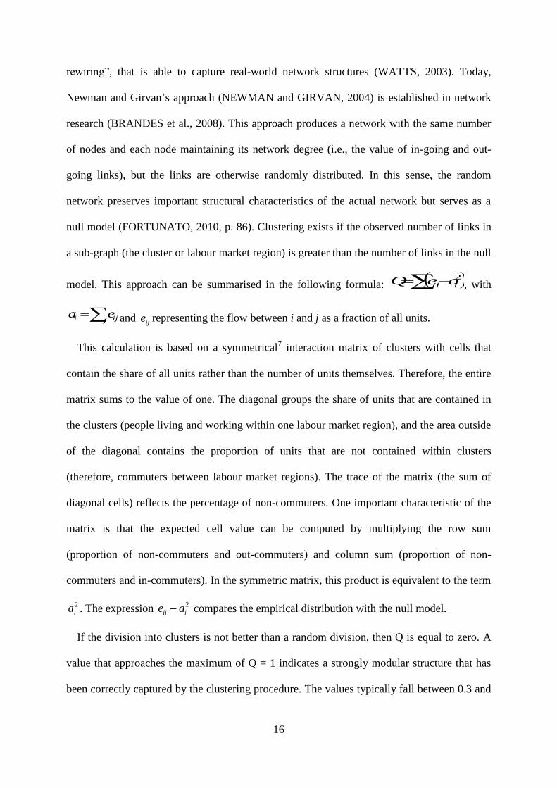
model. This approach can be summarised in the following formula: i iii aeQ 2

, with

j iji ea and ije representing the flow between i and j as a fraction of all units.

This calculation is based on a symmetrical7 interaction matrix of clusters with cells that

contain the share of all units rather than the number of units themselves. Therefore, the entire

matrix sums to the value of one. The diagonal groups the share of units that are contained in

the clusters (people living and working within one labour market region), and the area outside

of the diagonal contains the proportion of units that are not contained within clusters

(therefore, commuters between labour market regions). The trace of the matrix (the sum of

diagonal cells) reflects the percentage of non-commuters. One important characteristic of the

matrix is that the expected cell value can be computed by multiplying the row sum

(proportion of non-commuters and out-commuters) and column sum (proportion of non-

commuters and in-commuters). In the symmetric matrix, this product is equivalent to the term

2

ia . The expression 2

iii ae compares the empirical distribution with the null model.

If the division into clusters is not better than a random division, then Q is equal to zero. A

value that approaches the maximum of Q = 1 indicates a strongly modular structure that has

been correctly captured by the clustering procedure. The values typically fall between 0.3 and

17

0.7, in the wide array of areas in which network measures are applied. For commuting data, in

which high levels of clustering in agglomerations occur, comparatively higher values can be

expected. In a comparative study of the various procedures, KROPP and SCHWENGLER

(2008, pp. 40f.) achieved values that were well over 0.8. Such values are also found in the

delineation proposal that is presented in the next section. The advantage of maximising the

modularity measure in comparison to minimising commuter shares or maximising self-

containment (cf. section 5.5) is that the latter is only achieved by merging all regions into one

region, whereas the modularity approach uses an appropriate null model (cf. NEWMAN and

GIRVAN, 2004, p. 7).

After varieties of delineations have been defined using the modified dominant flow method

and an optimal delineation has been selected with the help of modularity values, the result is

further improved in a final optimisation process. This process serves the following three

purposes: it (re)assigns municipalities to labour market regions in accordance with their

strongest commuter flows; it corrects the labour market assignment for municipalities that are

completely surrounded by another labour market; and it assigns isolated municipalities with

no data or comparatively few commuters to the closest labour market region. If the previous

delineation process works well, these steps should result in minor changes. In the presented

case, we also use the optimisation procedure to generate the final delineation on municipal

level rather than municipal region level.

To conclude, the proposed delineation procedure can be summarised in the following

steps:

A. Cluster generator8 (results in section 5.1)

1. Compute a bidirectional flow matrix of all regions.

2. Compute the commuters' share of employees residing in the same region (row-wise

normalisation).

3. Select dominant flows, i.e.,

- strongest interaction that a region has with other regions,

- from a less to more populated region,

- above a certain threshold.

18

4. Merge regions that are connected by dominant flows.

> Continue with step 1 until no changes occur.

B. Selection (results in section 5.2)

Select the cluster solution with the highest modularity value Q.

C. Final optimisation process (results in section 5.3)

1. Ensure that each region is connected to the labour market region with which it

has the highest bidirectional flow.

2. Assign isolated municipal regions with no data or comparatively few

commuters to the closest labour market region.

3. Ensure regional coherence of labour market regions.

In principle, the cluster generator does not need to be based on the current procedure. It is

effective for various types of procedures. For example, cluster analysis and factor analysis

also provide cluster solutions. By comparing various methods the graph theoretical approach

has been more successful to produce delineations with strong interactions within labour

market regions and few connections to outside regions than other methods (KROPP and

SCHWENGLER, 2008). It is possible that we are not aware of all clustering procedures. In

network research, some promising modularity optimising methods are currently in

development. However, algorithms for valued graphs (WALTMAN et al., 2010; BLONDEL

et al., 2008) are not yet alternatives to the current approach.

5 Results

5.1 The cluster generator at work

Depending on the threshold value for the dominant flows and the number of iterations of the

algorithm, several labour market delineations are achieved. For the aggregated matrix NEW

(years 2006 to 2008), thresholds of 1% to 12% led to up to 7 iterations and more than 60

different cluster solutions. With a threshold of 1, the 2,000 municipal regions were merged

into 43 regions in one step (which includes merging all regions that are connected – directly

and indirectly – by dominant flows greater than 1% of the resident employed labour force)

and into only 4 regions after the second iteration. In contrast, with a threshold of 12%, the

process ended after 7 iterations, with 178 regions.

19

5.2 Choosing the analytically best delineation

Fig. 2 presents the modularity Q values for delineations resulting from different thresholds

and iterations for the aggregated matrix NEW (years 2006 to 2008). The values on the x-axis

represent the number of labour market regions that were generated by the cluster generator.

The lines mark the highest modularity (Q = 0.8447), which was achieved by merging the

municipal regions to form 51 labour market regions (applying a threshold of 7 and performing

4 iterations).

Fig. 2: Modularity Q values for different thresholds and iterations

Source: Authors' own illustration

Fig. 2 reveals several important characteristics. First, with the current data, very high

modularity values can be achieved only if the municipal regions are grouped into between 30

and 100 labour market regions. Rougher or significantly finer divisions achieve lower values

of Q. This finding also applies when other delineation procedures are employed (cf. KROPP,

2009). Second, in the case of low threshold values (dark circles), the municipal regions are

0.00

0.10

0.20

0.30

0.40

0.50

0.60

0.70

0.80

0.90

1.00

Mo

du

larity

Q

0 100 200 300 400 500No. of Labour Market Regions

Threshold = 1 ... Threshold > 8

20

quickly grouped into a few very large labour market regions. Hence, delineations with lower

threshold values tend to be located on the left side of Fig. 2. In contrast, very high threshold

values (light circles) stop the merging process at a point with many labour market regions and

very high modularity values have not yet been reached.

The delineation process that yielded the highest modularity (denoted by the thickest black

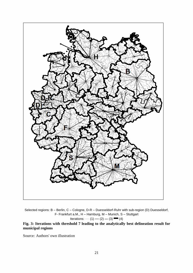
lines) is shown in the map of Germany in Fig. 3.9 Fig. 3 also shows the results of the first

three iterations (denoted by thinner lines), which produced smaller labour market regions. The

first iteration yielded 337 labour market regions, with a modularity of Q = 0.7502. The second

iteration produced 118 labour market regions and achieved a high modularity of Q = 0.8228.

After the third iteration, the quality of the division (Q = 0.8411 for 60 labour market regions)

differed only slightly from the best solution (Q = 0.8447 for 51 regions), which was obtained

after four iterations (see Table 4 in section 5.5. for a comparison with other quality measures).

21

Selected regions: B – Berlin, C – Cologne, D-R – Duesseldorf-Ruhr with sub-region (D) Duesseldorf,

F- Frankfurt a.M., H – Hamburg, M – Munich, S – Stuttgart

Iterations: –– (1) –– (2) ▬ (3) ▄▄▄

(4)

Fig. 3: Iterations with threshold 7 leading to the analytically best delineation result for

municipal regions

Source: Authors' own illustration

22

Fig. 3 also shows that monocentric regions (i.e., regions such as Hamburg, Berlin, and

Munich, which are dominated by a metropolis) grew particularly quickly. This result is

reasonable because the commuting flows were frequently directed towards one centre. In

polycentric regions such as the Ruhr area (see the Duesseldorf-Ruhr area in Fig. 3), however,

clearly dominant commuting flows were the exception. Nonetheless, the results also appear

plausible in these polycentric regions. After the first iterative step, very small-scale

delineations continued to dominate. However, after the second iteration, quite large-scale

labour markets were apparent. These regions grew further in the third iterative step. In the

fourth iteration, the Duesseldorf and Ruhr regions were merged into the labour market region

of Duesseldorf-Ruhr. The spatial structures revealed in this process are consistent with recent

regional studies (BLOTEVOGEL and SCHULZE, 2010, p. 268). Without an adequate

aggregation of both the concentrated commuting flows in monocentric regions and the more

network-like interactions in polycentric regions, it is impossible to achieve very high

modularity values for the delineation.

Of note, the parameters for the delineation (threshold value and number of iterations) were

not arbitrarily specified; instead, they were selected using a quality criterion, the modularity

value. The delineation that was eventually chosen comprised 51 labour market regions that

were quite heterogeneous in terms of size, which may not seem suitable for practical

applications at first sight.

5.3 Optimisation procedure

The final step ensured that each region was assigned to the labour market region with which it

had the strongest commuting interactions. By applying the correction procedure on a

municipal level (rather than a municipal region level), we produced a delineation on the

smallest regional level for which data were available. When necessary, the original

assignment was corrected by reassigning a municipal region to the regional labour market

23

with which it had the strongest relation. Because the reassignment of one municipality can

affect the assignment of neighbouring regions, this correction process was repeated until a

stable solution was achieved. During this procedure, approximately 6% of all municipalities,

with only 1.25% of the total labour force, were reassigned to a different labour market, and

the delineation was refined to the municipal level. These corrections also serve as a response

to the criticism that the assignment of elements to clusters in hierarchical cluster procedures is

not automatically corrected when the structure of the cluster changes. This should be a minor

problem in the presented approach because only a few iterations were necessary. The few

corrections10

that were required in the optimisation procedure indicated that the overall

clustering algorithm worked well.

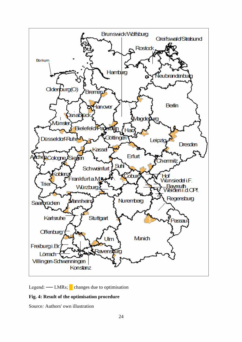
The optimisation procedure resulted in a delineation of 50 labour markets, which is shown

in Fig. 4. The resulting shift in the boundaries of the labour market regions was minimal, but

the modularity of the delineation increased slightly from Q = 0.8447 to Q = 0.8492.

24

Legend: ── LMRs; █ changes due to optimisation

Fig. 4: Result of the optimisation procedure

Source: Authors' own illustration

25

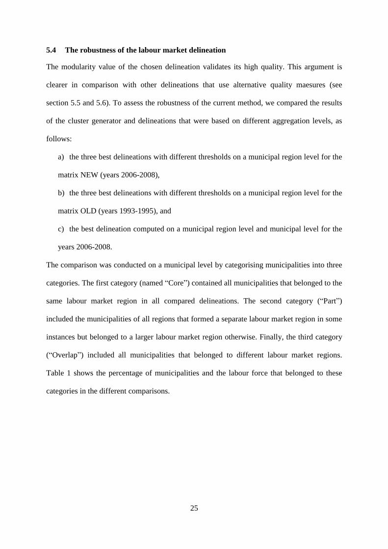
5.4 The robustness of the labour market delineation

The modularity value of the chosen delineation validates its high quality. This argument is

clearer in comparison with other delineations that use alternative quality maesures (see

section 5.5 and 5.6). To assess the robustness of the current method, we compared the results

of the cluster generator and delineations that were based on different aggregation levels, as

follows:

a) the three best delineations with different thresholds on a municipal region level for the

matrix NEW (years 2006-2008),

b) the three best delineations with different thresholds on a municipal region level for the

matrix OLD (years 1993-1995), and

c) the best delineation computed on a municipal region level and municipal level for the

years 2006-2008.

The comparison was conducted on a municipal level by categorising municipalities into three

categories. The first category (named “Core”) contained all municipalities that belonged to the

same labour market region in all compared delineations. The second category (“Part”)

included the municipalities of all regions that formed a separate labour market region in some

instances but belonged to a larger labour market region otherwise. Finally, the third category

(“Overlap”) included all municipalities that belonged to different labour market regions.

Table 1 shows the percentage of municipalities and the labour force that belonged to these

categories in the different comparisons.

26

Table 1: Robustness of the actual delineation

a) Three best delineations

with different thresholds for

the matrix NEW

b) Three best delineations

with different thresholds for

the matrix OLD

c) The best delineation

computed on municipal

region level and municipal

levels for the Matrix NEW

Category % of

municipalities

% of labour

force

% of

municipalities

% of labour

force

% of

municipalities

% of labour

force

Core 70.6 81.3 79.7 89.4 79.8 91.2

Part 20.4 15.1 13.3 8.3 10.0 5.8

Overlapping 9.0 3.6 6.9 2.3 10.2 3.0

Total 100.0 100.0 100.0 100.0 100.0 100.0

Note: Compared delineations were not optimised

According to the comparison, a vast majority of municipalities belonged to the same labour

market regions. Because these regions included most of the important labour market centres,

the percentage of the labour force within this category was even larger. The second category

(“Part”) was less problematic. Regions that belonged to one labour market region in some

cases but formed a separate region in other cases could be characterised as important sub-

regions of larger regions. The most problematic category, “Overlapping”, was comparatively

small.

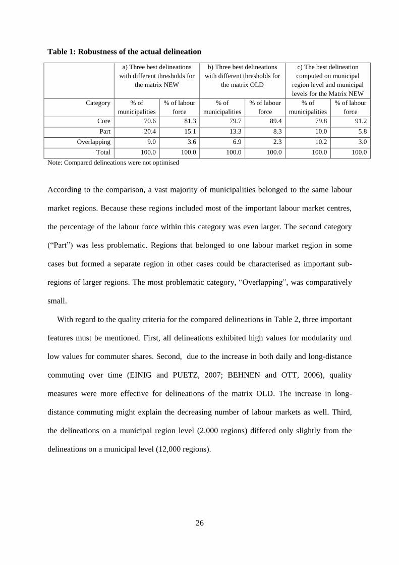
With regard to the quality criteria for the compared delineations in Table 2, three important

features must be mentioned. First, all delineations exhibited high values for modularity und

low values for commuter shares. Second, due to the increase in both daily and long-distance

commuting over time (EINIG and PUETZ, 2007; BEHNEN and OTT, 2006), quality

measures were more effective for delineations of the matrix OLD. The increase in long-

distance commuting might explain the decreasing number of labour markets as well. Third,

the delineations on a municipal region level (2,000 regions) differed only slightly from the

delineations on a municipal level (12,000 regions).

27

Table 2: Quality of delineations used in the comparisons

Number of labour

market regions

Modularity

Q

% of commuters between

labour market regions

a) Delineations of municipal region level for matrix NEW (2006-2008)

threshold: 7, iteration: 4, optimised 50 0.8492 10.2

threshold: 7, iteration: 4 a, c

51 0.8447 10.6

threshold: 5, iteration: 2 a 53 0.8443 10.4

threshold: 8, iteration: 7 a 63 0.8391 11.1

b) Delineations of municipal region level for matrix OLD (1993-1995)

threshold: 5, iteration: 3 b 66 0.8756 8.0

threshold: 4, iteration: 2 b 66 0.8756 7.8

threshold: 6, iteration: 4 b 84 0.8752 8.2

c) Delineations of municipal level for matrix NEW (2006-2008)

threshold: 7, iteration: 7, optimised 53 0.8477 9.9

threshold: 7, iteration: 7 c 54 0.8470 10.0

a, b,c – Delineations, used in the comparisons

5.5 Descriptive data

In this section, the optimised 50-labour-market delineation is described in greater detail and

compared with well-established delineations according to several characteristics. Table 3

presents a number of descriptive statistics for the ten largest (i.e., most populous) and smallest

(least populous) labour market regions of the optimised 50-labour-market delineation. The

most populous region was the Duesseldorf-Ruhr region, with 10 million inhabitants and over

3 million employees. This region accounted for over 12% of Germany's Gross Domestic

Product (GDP). The next largest regions, Munich, Frankfurt am Main, and Hamburg, had

approximately 6 million inhabitants each. The economic power of these regions was only

slightly smaller than that of the Duesseldorf-Ruhr region. Some of the least populous labour

market regions were located in Eastern Germany and Bavaria. An examination of the GDP

per capita and the unemployment rate revealed that labour market regions also differed

qualitatively.

28

In addition to the newly introduced modularity measure Q, the labour market regions’

commuting ratio and level of self-containment are well-established quality measures. The

commuting ratio is the ratio of in-commuters to out-commuters (in percentage). Values under

100 characterise regions with a surplus of outward commuters; values over 100 indicate that a

region has a surplus of inward commuters. For functional delineations, the figures should be

close to 100. Indeed, the larger labour market regions appeared to be quite balanced. Self-

containment measures the percentage of the employed local labour force that works in a

region. It can reach a maximum of 100%. In practice, however, there is always a certain

percentage of out-commuters, which reduces the self-containment values. Therefore, values of

approximately 90%, as in the present delineation, indicate a successful delineation result,

especially when compared to other delineations (Table 4).

29

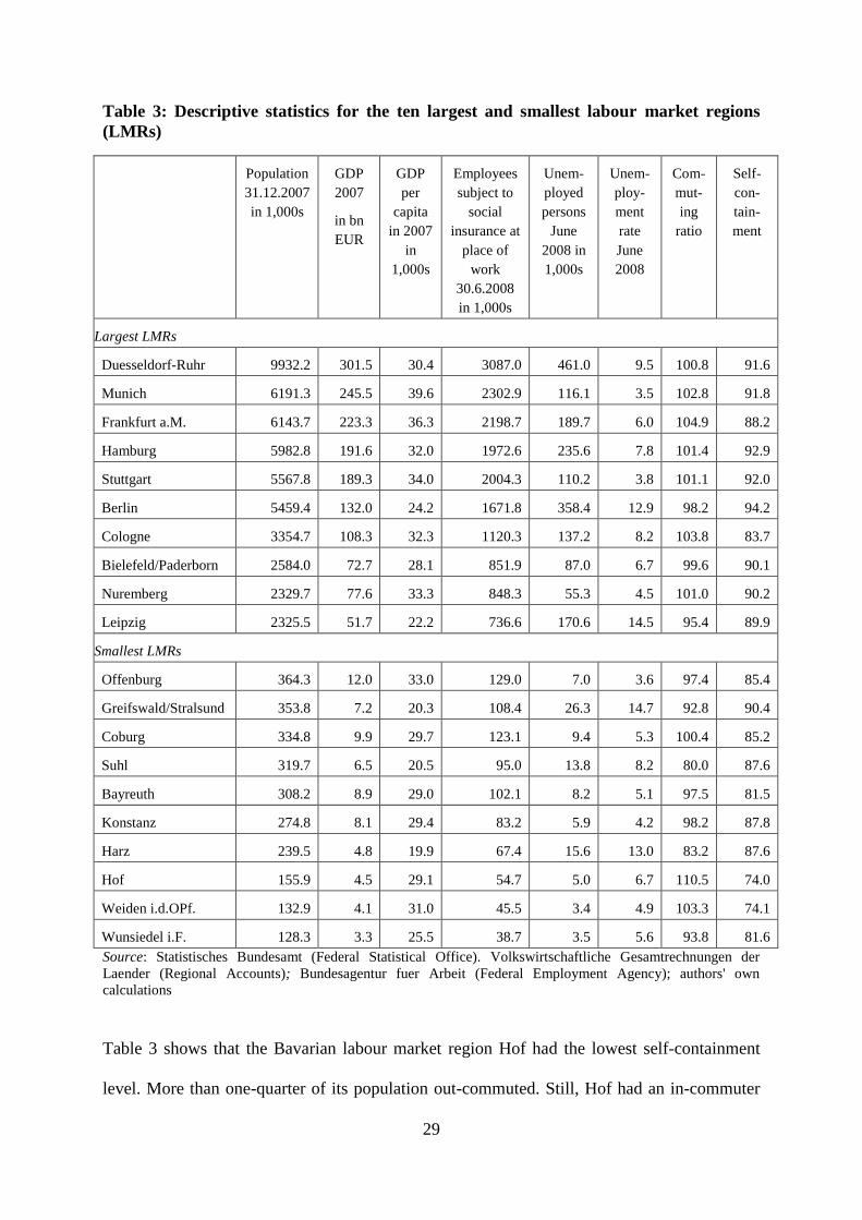
Table 3: Descriptive statistics for the ten largest and smallest labour market regions

(LMRs)

Population

31.12.2007

in 1,000s

GDP

2007

in bn

EUR

GDP

per

capita

in 2007

in

1,000s

Employees

subject to

social

insurance at

place of

work

30.6.2008

in 1,000s

Unem-

ployed

persons

June

2008 in

1,000s

Unem-

ploy-

ment

rate

June

2008

Com-

mut-

ing

ratio

Self-

con-

tain-

ment

Largest LMRs

Duesseldorf-Ruhr 9932.2 301.5 30.4 3087.0 461.0 9.5 100.8 91.6

Munich 6191.3 245.5 39.6 2302.9 116.1 3.5 102.8 91.8

Frankfurt a.M. 6143.7 223.3 36.3 2198.7 189.7 6.0 104.9 88.2

Hamburg 5982.8 191.6 32.0 1972.6 235.6 7.8 101.4 92.9

Stuttgart 5567.8 189.3 34.0 2004.3 110.2 3.8 101.1 92.0

Berlin 5459.4 132.0 24.2 1671.8 358.4 12.9 98.2 94.2

Cologne 3354.7 108.3 32.3 1120.3 137.2 8.2 103.8 83.7

Bielefeld/Paderborn 2584.0 72.7 28.1 851.9 87.0 6.7 99.6 90.1

Nuremberg 2329.7 77.6 33.3 848.3 55.3 4.5 101.0 90.2

Leipzig 2325.5 51.7 22.2 736.6 170.6 14.5 95.4 89.9

Smallest LMRs

Offenburg 364.3 12.0 33.0 129.0 7.0 3.6 97.4 85.4

Greifswald/Stralsund 353.8 7.2 20.3 108.4 26.3 14.7 92.8 90.4

Coburg 334.8 9.9 29.7 123.1 9.4 5.3 100.4 85.2

Suhl 319.7 6.5 20.5 95.0 13.8 8.2 80.0 87.6

Bayreuth 308.2 8.9 29.0 102.1 8.2 5.1 97.5 81.5

Konstanz 274.8 8.1 29.4 83.2 5.9 4.2 98.2 87.8

Harz 239.5 4.8 19.9 67.4 15.6 13.0 83.2 87.6

Hof 155.9 4.5 29.1 54.7 5.0 6.7 110.5 74.0

Weiden i.d.OPf. 132.9 4.1 31.0 45.5 3.4 4.9 103.3 74.1

Wunsiedel i.F. 128.3 3.3 25.5 38.7 3.5 5.6 93.8 81.6

Source: Statistisches Bundesamt (Federal Statistical Office). Volkswirtschaftliche Gesamtrechnungen der

Laender (Regional Accounts); Bundesagentur fuer Arbeit (Federal Employment Agency); authors' own

calculations

Table 3 shows that the Bavarian labour market region Hof had the lowest self-containment

level. More than one-quarter of its population out-commuted. Still, Hof had an in-commuter

30

surplus of 10%. Both values indicate that a labour market delineation was difficult for this

region.

5.6 Comparison with other delineations

Compared with the other delineations, the quality of the current study’s procedure is manifest

(Table 4). The percentage of people who crossed labour market boundaries (the column

“Commuters”11

) was by far the lowest in the presented 50-labour-market delineation. The

average commuting ratio and the self-containment values of the present delineation were

considerably higher than were those of the well-established delineations.12

Moreover, the

standard deviation of the commuting ratios was considerably smaller than were those of the

other delineations. Particularly, the high variance of values for the commuting ratio and the

low minimum values for self-containment of the other delineations indicate that there were at

least some less-than-ideal delineated regions. These shortcomings also occurred because all of

these delineations considered certain constraints, such as following district borders, minimum

sizes, and maximum commuting times. However, in an earlier comparison (KROPP and

SCHWENGLER, 2008), we applied these methods without further restrictions like maximum

commuting times or minimum sizes and came to similar conclusions.

31

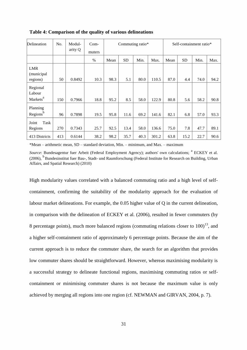
Table 4: Comparison of the quality of various delineations

Delineation No. Modul-

arity Q

Com-

muters

Commuting ratio* Self-containment ratio*

% Mean SD Min. Max. Mean SD Min. Max.

LMR

(municipal

regions) 50 0.8492 10.3 98.3 5.1 80.0 110.5 87.0 4.4 74.0 94.2

Regional

Labour

Marketsa 150 0.7966 18.8 95.2 8.5 58.0 122.9 80.8 5.6 58.2 90.8

Planning

Regionsb

96 0.7898 19.5 95.8 11.6 69.2 141.6 82.1 6.8 57.0 93.3

Joint Task

Regions 270 0.7343 25.7 92.5 13.4 58.0 136.6 75.0 7.8 47.7 89.1

413 Districts 413 0.6144 38.2 98.2 35.7 40.3 301.2 63.8 15.2 22.7 90.6

*Mean – arithmetic mean, SD – standard deviation, Min. – minimum, and Max. – maximum

Source: Bundesagentur fuer Arbeit (Federal Employment Agency); authors' own calculations; a ECKEY et al.

(2006), b

Bundesinstitut fuer Bau-, Stadt- und Raumforschung (Federal Institute for Research on Building, Urban

Affairs, and Spatial Research) (2010)

High modularity values correlated with a balanced commuting ratio and a high level of self-

containment, confirming the suitability of the modularity approach for the evaluation of

labour market delineations. For example, the 0.05 higher value of Q in the current delineation,

in comparison with the delineation of ECKEY et al. (2006), resulted in fewer commuters (by

8 percentage points), much more balanced regions (commuting relations closer to 100)13

, and

a higher self-containment ratio of approximately 6 percentage points. Because the aim of the

current approach is to reduce the commuter share, the search for an algorithm that provides

low commuter shares should be straightforward. However, whereas maximising modularity is

a successful strategy to delineate functional regions, maximising commuting ratios or self-

containment or minimising commuter shares is not because the maximum value is only

achieved by merging all regions into one region (cf. NEWMAN and GIRVAN, 2004, p. 7).

32

The present study shows that a delineation of commuting areas with high modularity values

and low inter-regional commuter shares comprises approximately 30-75 labour market

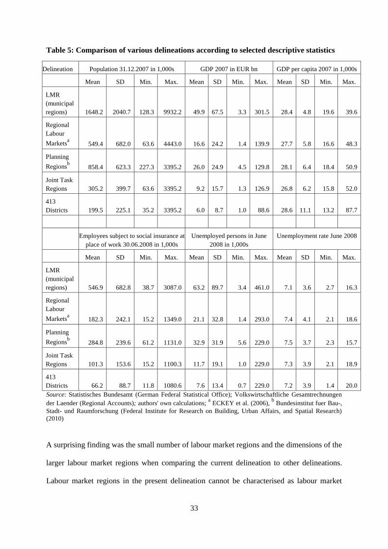
regions (cf. Fig. 2). Other descriptive data in Table 5 show the heterogeneity of the labour

market regions in terms of size. Labour market regions with high modularity values were

considerably more heterogeneous in terms of size than the established functional delineations,

as confirmed by the large standard deviations for population, GDP, the number of employed

persons being subject to the compulsory social security scheme, and the number of

unemployed persons. By implication, with our data a labour market delineation that

minimises commuting interactions between functional regions cannot be homogeneous in

terms of size, although this is often required in the interests of practical applicability.

33

Table 5: Comparison of various delineations according to selected descriptive statistics

Delineation Population 31.12.2007 in 1,000s GDP 2007 in EUR bn GDP per capita 2007 in 1,000s

Mean SD Min. Max. Mean SD Min. Max. Mean SD Min. Max.

LMR

(municipal

regions) 1648.2 2040.7 128.3 9932.2 49.9 67.5 3.3 301.5 28.4 4.8 19.6 39.6

Regional

Labour

Marketsa 549.4 682.0 63.6 4443.0 16.6 24.2 1.4 139.9 27.7 5.8 16.6 48.3

Planning

Regionsb

858.4 623.3 227.3 3395.2 26.0 24.9 4.5 129.8 28.1 6.4 18.4 50.9

Joint Task

Regions 305.2 399.7 63.6 3395.2 9.2 15.7 1.3 126.9 26.8 6.2 15.8 52.0

413

Districts 199.5 225.1 35.2 3395.2 6.0 8.7 1.0 88.6 28.6 11.1 13.2 87.7

Employees subject to social insurance at

place of work 30.06.2008 in 1,000s

Unemployed persons in June

2008 in 1,000s

Unemployment rate June 2008

Mean SD Min. Max. Mean SD Min. Max. Mean SD Min. Max.

LMR

(municipal

regions) 546.9 682.8 38.7 3087.0 63.2 89.7 3.4 461.0 7.1 3.6 2.7 16.3

Regional

Labour

Marketsa 182.3 242.1 15.2 1349.0 21.1 32.8 1.4 293.0 7.4 4.1 2.1 18.6

Planning

Regionsb

284.8 239.6 61.2 1131.0 32.9 31.9 5.6 229.0 7.5 3.7 2.3 15.7

Joint Task

Regions 101.3 153.6 15.2 1100.3 11.7 19.1 1.0 229.0 7.3 3.9 2.1 18.9

413

Districts 66.2 88.7 11.8 1080.6 7.6 13.4 0.7 229.0 7.2 3.9 1.4 20.0

Source: Statistisches Bundesamt (German Federal Statistical Office); Volkswirtschaftliche Gesamtrechnungen

der Laender (Regional Accounts); authors' own calculations; a ECKEY et al. (2006),

b Bundesinstitut fuer Bau-,

Stadt- und Raumforschung (Federal Institute for Research on Building, Urban Affairs, and Spatial Research) (2010)

A surprising finding was the small number of labour market regions and the dimensions of the

larger labour market regions when comparing the current delineation to other delineations.

Labour market regions in the present delineation cannot be characterised as labour market

34

centres and their adjacent hinterlands. Instead, the regions are large-scale areas that are

characterised by a dense network of direct and indirect commuting flows. For example,

whereas many workers commute to large cities such as Munich from the city's more distant

hinterland, accepting above-average commuting distances and home-to-office times (cf.

BUNDESAMT FUER BAUWESEN UND RAUMORDNUNG, 2005), a large number of

commuters travel from the hinterland to neighbouring labour market centres and vice versa.

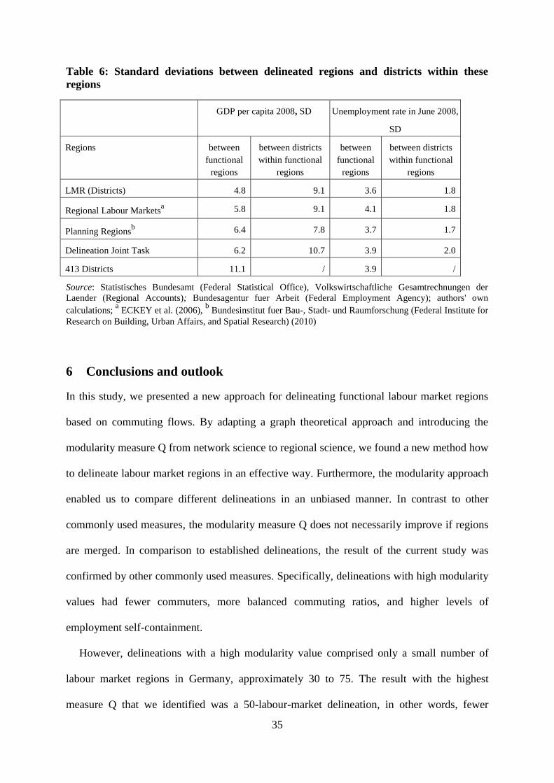
Finally, we investigated whether functionally delineated labour market regions are also

more economically homogeneous in terms of GDP per capita or unemployment rate than

administrative regions (Table 6). The first column for each indicator provides the standard

deviations between the regions, which are also provided in Table 5. The next column shows

the average standard deviations for all districts within the delineations. Because the

calculations were based on district-level data, a variant form of the 50-labour-market

delineation was used in this comparison. In both examples, the standard deviations were

indeed smaller between districts within functional regions than across all 413 districts. The

50-labour-market delineation did not always achieve the best values. However, the small

standard deviations were remarkable because relatively homogeneous regions could be

generated with the help of a very rough delineation or one that comprised comparatively few

regions.

35

Table 6: Standard deviations between delineated regions and districts within these

regions

GDP per capita 2008, SD Unemployment rate in June 2008,

SD

Regions between

functional

regions

between districts

within functional

regions

between

functional

regions

between districts

within functional

regions

LMR (Districts) 4.8 9.1 3.6 1.8

Regional Labour Marketsa 5.8 9.1 4.1 1.8

Planning Regionsb 6.4 7.8 3.7 1.7

Delineation Joint Task 6.2 10.7 3.9 2.0

413 Districts 11.1 / 3.9 /

Source: Statistisches Bundesamt (Federal Statistical Office), Volkswirtschaftliche Gesamtrechnungen der

Laender (Regional Accounts); Bundesagentur fuer Arbeit (Federal Employment Agency); authors' own

calculations; a ECKEY et al. (2006),

b Bundesinstitut fuer Bau-, Stadt- und Raumforschung (Federal Institute for

Research on Building, Urban Affairs, and Spatial Research) (2010)

6 Conclusions and outlook

In this study, we presented a new approach for delineating functional labour market regions

based on commuting flows. By adapting a graph theoretical approach and introducing the

modularity measure Q from network science to regional science, we found a new method how

to delineate labour market regions in an effective way. Furthermore, the modularity approach

enabled us to compare different delineations in an unbiased manner. In contrast to other

commonly used measures, the modularity measure Q does not necessarily improve if regions

are merged. In comparison to established delineations, the result of the current study was

confirmed by other commonly used measures. Specifically, delineations with high modularity

values had fewer commuters, more balanced commuting ratios, and higher levels of

employment self-containment.

However, delineations with a high modularity value comprised only a small number of

labour market regions in Germany, approximately 30 to 75. The result with the highest

measure Q that we identified was a 50-labour-market delineation, in other words, fewer

36

regions than the well-established delineations. These 50 labour market regions were quite

heterogenous in their terms of size. Especially around cities such as Hamburg, Berlin,

Munich, and Frankfurt (Main), complex commuting patterns led to large labour market

regions. These large agglomerations cannot be characterised as dominant centres and

immediate commuter belts. Commuting flows between sub-centres within the hinterland and

between the hinterland and the periphery also play an important role. Even if the labour

market regions transcend the boundaries of commuter belts, they constitute a common labour

market. In the medium term, changes in one part of this labour market are likely to affect

other areas that are weakly linked to or distant from the area in which these changes occur.

We also demonstrated that established functional delineations do not always appropriately

capture important commuting relations between regions, as observed from the significantly

higher commuter shares in the case of delineations that comprised a large number of regions.

This is especially true for delineations that are subject to certain restrictions such as minimum

size, maximum commuter times within delimited regions, and consistency with administrative

boundaries. The labour markets of the city states of Hamburg, Berlin, and Bremen were

distinctly larger than their own federal state boundaries. If the German federal state

boundaries are utilised, these important economic centres are cut off from their hinterlands.

Without a coordinated labour market and economic policy that transcends federal state

boundaries, important labour market issues cannot be tackled successfully.

The identified heterogeneity of regional labour markets is important for regional policy. As

labour markets around metropolitan centers are larger than they are presented in established

delineations, the number of regions that should coordinate their regional labour policy is

larger as well. Conversely, the development of very small functional regions might be

hampered by the regions’ insufficient size. It might be a challenge for labour market and

economic policy to manage these different labour market regions and determine which

37

administrations should cooperate with each other. In general, the observed heterogeneity is

not surprising in light of the dynamics of aggregation processes in recent decades. If the

mobility of goods and labour is decreasingly restricted by distance, agglomeration processes

might speed up and increase heterogeneity. The creation of metropolitan areas in Germany

since 1995 is certainly one attempt to cope with the reality of large functional regions. How

such heterogeneous regions may serve as an appropriate basis for regional science must be

examined by future research. The heterogeneity itself might be an explanation for differences

in regional development. Conversely, a comparison of larger regions could be more valid if

based on the current proposal for labour market delineations.

We claim that the current three-step-method facilitates the delineation of functional regions

in a manner that captures spatial interaction flows more effectively than previous attempts. In

this way, the current approach provides a new answer to the question “What is a region?” and

might help define functional regions that are an appropriate foundation for regional analyses.

7 References

BEHNEN T. and OTT E. (2006) Arbeitskraeftemobilitaet – Fernpendler und ihre

Lebenssituation, in: LEIBNIZ-INSTITUT FUER LAENDERKUNDE (Ed) Nationalatlas

Bundesrepublik Deutschland – Arbeit und Lebensstandard, 56-59.

BLONDEL V. D., GUILLAUME J.-L., LAMBIOTTE R., LEFEBVRE E. (2008) Fast

unfolding of communities in large networks, Journal of Statistical Mechanics: Theory and

Experiment 2008 (10), P10008.

BLOTEVOGEL H. H. (1996) Zur Kontroverse um den Stellenwert des Zentralen-Orte-

Konzepts in der Raumordnungspolitik heute, Informationen zur Raumentwicklung, 10,

647-657.

38

BLOTEVOGEL H. H. (2005) Zentrale Orte, Handwoerterbuch der Raumordnung der ARL,

1307-1315.

BLOTEVOGEL H. H. and SCHULZE K. (2010) 1 oder 2 oder 3? Zur Konstituierung

moeglicher Metropolregionen an Rhein und Ruhr, Raumforschung und Raumordnung

68(4), 255-270.

BODE E. (2008) Delineating Metropolitan Areas using Land Prices, Journal of Regional

Science 48(1), 131-163.

BONGAERTS D., COERVERS F. and HENSEN M. (2004) The Delimitation and Coherence

of Functional and Administrative Regions, Research Series 04O19, Ministry of Economic

Affairs, The Hague.

BRANDES U., DELLING D., GAERTLER M., GÖRKE R., HOEFER M., NIKOLOSKI Z.,

WAGNER D. (2008): On Modularity Clustering. IEEE Transactions on Knowledge and

Data Engineering, 20, pp. 172-188.

BUNDESAGENTUR FUER ARBEIT (2008) Der Arbeits- und Ausbildungsmarkt in

Deutschland, Monatsbericht Dezember und das Jahr 2008, Nuremberg.

BUNDESAMT FUER BAUWESEN UND RAUMORDNUNG (2005) Raumordnungsbericht

2005, Bonn.

BUNDESINSTITUT FUER BAU-, STADT- UND RAUMFORSCHUNG (BBSR) IM

BUNDESAMT FUER BAUWESEN UND RAUMORDNUNG (BBR) (2010)

Raumordnungsregionen (Analyseraeume).

(http://www.bbsr.bund.de/cln_016/nn_103086/BBSR/DE/Raumbeobachtung/Werkzeuge/R

aumabgrenzungen/Raumordnungsregionen/raumordnungsregionen.html; accessed 1 April

2010).

CASADO-DÍAZ J. M. (2000) Local labour market areas in Spain: a case study, Regional

Studies 34(9), 843-856.

39

CASTELLS M (1996) The rise of the network society. Blackwell, Oxford

CHRISTALLER W. (1933, reprint 1968) Die zentralen Orte in Sueddeutschland, Jena,

Darmstadt.

COERVERS F., HENSEN M. and BONGAERTS D. (2009) Delimitation and Coherence of

Functional and Administrative Regions Regional Studies 43(1), 19-31.

COOMBES M. G., GREEN A. E. and OPENSHAW S. (1986) An efficient algorithm to

generate official statistical reporting areas: the case of the 1984 travel-to-work areas

revision in Britain, Journal of the Operational Research Society 37(10), 943-953.

DAUTH W. (2010) The mysteries of the trade: employment effects of urban interindustry

spillovers, IAB-Discussion Paper, No. 15/2010, Nuremberg.

ECKEY H.-F. (1988) Abgrenzung regionaler Arbeitsmaerkte, Raumforschung und

Raumordnung 46(1-2), 24-33.

ECKEY H.-F., KOSFELD R. and TUERCK M. (2006) Abgrenzung deutscher

Arbeitsmarktregionen, Raumforschung und Raumordnung 64(4), 299-309.

EINIG K. and PUETZ T. (2007) Regionale Dynamik der Pendlergesellschaft. Entwicklung

von Verflechtungsmustern und Pendeldistanzen, Informationen zur Raumentwicklung 2/3,

73-91.

FORTUNATO S. (2010) Community detection in graphs, Physics Reports 486(3-5), 75-174.

GIRVAN M. and NEWMAN M. E. J. (2002) Community structure in social and biological

networks. Proceedings of the National Academy of Sciences of the United States of

America PNAS 99 (12): 7821–7826.

GLÜCKLER J. (2007) Economic geography and the evolution of networks, Journal of

Economic Geography 7(5), 619-634

GORMAN S. P., PATUELLI R., REGGIANI A., NIJKAMP P., KULKARNI R. and HAAG,

G. (2007) An Application of Complex Network Theory to German Commuting Patterns, in

40

FRIESZ, T. L. (Ed) Network Science, Nonlinear Science and Infrastructure Systems, pp.

167-185, Springer-Verlag, Berlin.

HAAG G. and BINDER J. (2001) Endbericht zum Forschungsprojekt “Vergleichende

Untersuchung der Wirkungszusammenhaenge zwischen Pendelverkehr und der

raeumlichen Organisationsstruktur der Region Stuttgart und der Provinz Turin”.

Sonderauswertung der Ergebnisse des VIGONI-Projekts im Auftrag des Verbandes Region

Stuttgart. Stuttgart, November 2001.

HENSEN M. and COERVERS F. (2003) The regionalization of labour markets by modelling

commuting behaviour. (http://www.roa.unimaas.nl/seminars/pdf2005/M.Hensen.pdf;

accessed 26 January 2010).

JONES M. / PAASI A. (2013) Regional World(s): Advancing the Geography of Regions,

Regional Studies. 47(1),. 1-5.

KARLSSON Ch. and OLSSON M. (2006) The identification of functional regions: theory,

methods, and applications, Annals of Regional Science 40(1), 1-18.

KLEMMER P. and KRAEMER D. (1975) Regionale Arbeitsmaerkte. Ein

Abgrenzungsvorschlag fuer die Bundesrepublik Deutschland, Beitraege zur Struktur- und

Konjunkturforschung, Band 1, Brockmeyer-Verlag, Bochum.

KOSFELD R. and WERNER A. (2012) Deutsche Arbeitsmarktregionen – Neuabgrenzung

nach den Kreisgebietsreformen 2007-2011, Raumforschung und Raumordnung, 70(1), 49-

64.

KROPP P. (2009) Die Abgrenzung der Arbeitsmarktregion Bremen, IAB-Regional

No. 3/2009, Nuremberg.

KROPP P. and SCHWENGLER B. (2008) Abgrenzung von Wirtschaftsraeumen auf der

Grundlage von Pendlerverflechtungen. Ein Methodenvergleich, IAB-Discussion Paper

No. 41/2008, Nuremberg.

41

KROPP P. and SCHWENGLER B. (2011) Abgrenzung von Arbeitsmarktregionen - ein

Methodenvorschlag, Raumforschung und Raumordnung 69(1), 45-62. DOI

10.1007/s13147-011-0076-4.

KRUGMAN P. (1991) Geography and trade, Cambridge (Mass.), MIT Press.

LOESCH A. (1940, reprint 1962) Die raeumliche Ordnung der Wirtschaft, Jena, Stuttgart.

MADELIN M., GRASLAND C., MATHIAN H., SANDERS L. and VINCENT J.-M. (2009)

Das “MAUP”: Modiable Areal Unit – Problem oder Fortschritt? Informationen zur

Raumentwicklung 10/11, 645-660.

MARSHALL A. (1890) Principles of Economics, Macmillan, London.

NEWMAN M. E. J. (2003) Mixing patterns in networks, Physical Review E 67 026126.

NEWMAN M. E. J. and GIRVAN M. (2004) Finding and evaluating community structure in

networks, Physical Review E 69 026113.

NYSTUEN J. D. and DACEY M. F. (1961) A Graph Theory Interpretation of Nodal Regions,

Papers and Proceedings of the Regional Science Association 7(1), 29-42.

OFFICE FOR NATIONAL STATISTICS (ONS) and COOMBES M. G. (1998) 1991-based

Travel-to-Work Areas, Office for National Statistics, London.

OPENSHAW S. (1984) The modifiable areal unit problem, Norwich, Geo Books.

PALLA G., DERÉNYI I., FARKAS I. and VICSEK T. (2005) Uncovering the overlapping

community structure of complex networks in nature and society. Nature 435 (7043): 814–

818.

RABINO G. A. and OCCELLI S. (1997) Understanding spatial structure from network data:

theoretical considerations and applications. Cybergeo, Systèmes, Modélisation,

Géostatistiques, article 29, mis en ligne le 26 juin 1997, modifié le 21 avril 2008.

(http://www.cybergeo.eu/index2199.html; accessed 27 January 2010).

42

RAPOPORT A. (1957) Contribution to the theory of random and biased nets, The bulletin of

mathematical biophysics 19(4), 257-277.

SMART M. W. (1974) Labour market areas: Uses and definition, Progress in Planning 2,

239-353.

TER WAL A. L. J. and BOSCHMA R. A. (2009) Applying social network analysis in

economic geography: framing some key analytic issues. The Annals of Regional Science

43(3), 739-756.

TOLBERT Ch. M. and KILIAN M. S. (1987) Labor Market Areas for the United States. Staff

Report. Washington, D.C.: USDA, ERS, Agriculture and Rural Economy Division.

VAN NUFFEL N. (2007) Determination of the Number of Significant Flows in Origin –

Destination Specific Analysis: The Case of Commuting in Flanders, Regional Studies

41(4), 509-524.

VAN DER LAAN L. and SCHALKE R. (2001) Reality versus Policy: The Delineation and

Testing of Local Labour Market and Spatial Policy Areas, European Planning Studies 9,

201-221.

WALTMAN L., VAN ECK N. J. and NOYONS E. C. M. (2010) A unified approach to

mapping and clustering of bibliometric networks, Journal of Informetrics, 4, 629-635.

WATTS D. J. (2003) Six Degrees: The Science of a Connected Age. New York, Norton.

8 Endnotes

1 In this comparison, we applied all methods without restrictions like maximum commuting times or minimum

sizes.

2 See SMART (1974, pp. 252ff.) for early examples.

3 Finding groups – nodes or units that are strongly related to each other – in networks has become an important

subject in the study of complex networks (cf. GIRVAN and NEWMAN, 2002; PALLA et al., 2005).

43

4 Nevertheless, analyses based on all 12,000 municipalities to control the used method have confirmed the

robustness of the results (section 5.4).

5 In this way, the current procedure is similar to that used by RABINO and OCCELLI (1997). These

researchers combined the graph theory approach with the threshold value procedure using threshold values

for the minimum magnitude of the dominant commuting flows and the minimum size of the catchment areas

(measured in terms of inhabitants and the number of municipalities). Tree graphs are formed only by

commuting flows that exceed a certain threshold. HAAG and BINDER (2001) also used this extended

concept for spatial analyses in the Stuttgart and Turin areas.

6 Fig. 3 (section 5.2) demonstrates the iteration process with a threshold of 7.

7 We used a symmetric interaction matrix as described in the original paper of NEWMAN and GIRVAN

(2004, p. 7) and implemented in standard software packages for network analysis as Pajek, ucinet or R.

However, it would be possible to employ NEWMAN’s (2003, p. 2) paper on assortative mixing, in which an

asymmetric case was discussed, and specify i jiii baeQ with j iji ea and i jij eb . We

thank Michał Bojanowski for recommending this solution. As inflow and outflow of our labour market

regions appear to be very balanced, the authors relay on the established formula.

8 Methods other than the current graph theoretical approach can be used as a cluster generator rather than or in

addition to this approach.

9 As a rule, the labour market regions were named after the municipality or municipal region that was the

terminal point of the sub-graph. Only in cases in which this name did not typify the labour market region, a

more appropriate label was chosen.

10 The island of Borkum was merged with the labour market region Oldenburg because it would otherwise form

an exceptionally small labour market. Two municipalities with insufficient data and three misplaced

municipalities with fewer than 500 employees total were assigned to a surrounding labour market region.

Misplacements may result from data problems; however, in some cases, municipalities were most strongly

connected to another (nearby) labour market region than all of their neighbours.

11 Here, the share of commuters (employees who live and work in different labour market regions) of all

employees was computed.

44

12

The commuting ratio between labour market regions should generally decrease, and the level of self-

containment should generally increase with fewer labour market regions. The measure Q, however, does not

have such a bias. One could argue that these results are due to the small number of labour market regions

rather than the method. However, the current cluster generator produced delineations with comparable

numbers of labour markets but with higher modularity values and lower commuting ratios (e.g., a 99-region-

delimitation with Q=0.8304 and 13.6% commuters, a 153-region-delimitation with Q=0.8133 and 15.8%

commuters, and a 274-region-delimitation with Q=0.7640 and 22.0% commuters, see also Fig. 2).

13 The values on a district-level delineation were also close to 100 but had a much higher standard deviation.