WORKING PAPERS

73

Mária Širaňová – Menbere Workie Tiruneh

THE DETERMINANTS OF ERRORS

AND OMISSIONS IN A SMALL

AND OPEN ECONOMY:

THE CASE OF SLOVAKIA

ISSN 1337-5598 (elektronická verzia)

Edícia WORKING PAPERS prináša priebežné, čiastkové výsledky výskumných prác pracovníkov alebo tímov EÚ SAV riešených v rámci výskumných projektov, ktoré môžu byť obsahom aj ďalších publikácií.

AUTORI

Ing. Mária Širaňová, PhD., M.A.

prof. Dr. Ing. Menbere Workie Tiruneh, PhD. RECENZENTI

doc. Ing. Juraj Sipko, PhD., MBA.

doc. Ing. Jana Kotlebová, PhD. ABSTRACT

The determinants of errors and omissions in a small and open economy: The case of Slovakia

This paper aims to empirically explore dynamics of the Net errors and omissions in a small and open economy of Slovakia. Data on the Net errors and omissions during the 2008-2014 period, which is known as the Great Recession, seem to suggest that the change in trend has been predominantly a phenomenon of real economy, mainly the service sector. Even though the paper does not find evidence of illicit financing (hot money flows) during the period under investigation the link between evolution of foreign direct investments and the NeO might point to a possible tax optimization. Likewise, our estimates have not confirmed existence of a connection between the dynamics of NeO and trade misinvoicing for goods during the peri-od. Given the absence of detailed bidirectional data on the service sector, the results need fur-ther empirical investigation to determine the true extent of the impact of service sector on the NeO item. KEYWORDS: balancing item of balance of payments, net errors and omissions, illicit capital

flows ABSTRAKT

Determinanty položky Chyby a omyly platobnej bilancie v malej otvorenej ekonomike: Slovensko ako prípadová štúdia

Cieľom tejto štúdie je vyšetriť dynamiku vývoja položky platobnej bilancie Chyby a omyly v malej otvorenej ekonomike Slovenska. Analýza dát týkajúcich sa rokov 2008 – 2014, ktoré časovo spadajú do obdobia tzv. Veľkej recesie, naznačuje, že zmena v trende tejto položky nastala prevažne z dôvodu pohybov v reálnom sektore, a to predovšetkým v obchode so služ-bami. Aj keď táto štúdia nenachádza významný vplyv tzv. nelegálneho presunu špeku-latívneho kapitálu („hot money“ flow) na položku Chýb a omylov počas sledovaného ob-dobia, existujúce prepojenie medzi vývojom priamych zahraničných investícií a danou položkou môže naznačovať prítomnosť daňovej optimalizácie. Zároveň nie je možné potvrdiť existenciu vzťahu medzi dynamikou vyrovnávajúcej položky a fenoménu zámerného pod alebo nadhodnocovania hodnoty export a importu v sektore tovarov. Vzhľadom na to, že de-tailnejšie informácie týkajúce sa sektora služieb v oblasti zámerného pod alebo nadhodnoco-vania export a importu nie sú v súčasnosti dostupné, skutočný vplyv obchodu so službami na položku chýb a omylov nie je možné bližšie špecifikovať. KĽÚČOVÉ SLOVÁ: vyrovnávajúca položka platobnej bilancie, chyby a omyly, nelegálne kapitá-

lové toky JEL CLASSIFICATION: F32, F41 Za obsah a jazykovú úroveň zodpovedajú autori.

Technické spracovanie: Mária Lacková

3

Ekonomický ústav SAV, Šancová 56, 811 05 Bratislava, www.ekonom.sav.sk

KONTAKT: maria.siranova@savba.sk; menbere.workie@savba.sk © Ekonomický ústav SAV, Bratislava 2015

O B S A H

INTRODUCTION ............................................................................................................................ 5

1. LITERATURE REVIEW ................................................................................................................ 8

2. METHODOLOGY .................................................................................................................... 11

2.1. UNIT ROOT TESTS ......................................................................................................................... 11

2.2. TESTS FOR STRUCTURAL BREAKS ...................................................................................................... 12

2.3. ARDL BOUND TEST ....................................................................................................................... 12

3. DATA DESCRIPTION AND LIST OF EXPLANATORY VARIABLES ................................................... 15

4. EMPIRICAL RESULTS ............................................................................................................... 16

4.1. STATISTICAL PROPERTIES ................................................................................................................ 18

4.2. ARDL MODEL OUTCOMES .............................................................................................................. 22

5. FOUR STORIES BEHIND THE TRENDING BALANCING ITEM ....................................................... 29

5.1. FOREIGN TRADE IN GOODS AND SERVICES ......................................................................................... 29

5.1.1. Cross-border vs national concept in trade statistics ....................................................... 32

5.2. CROSS-BORDER AND SEASONAL WORK AND ECONOMIC CRISIS .............................................................. 32

5.3. FOREIGN DIRECT INVESTMENTS ABROAD ........................................................................................... 33

5.4. PURE FINANCIAL SPECULATION AND RISE OF LONG-TERM CREDIT........................................................... 37

CONCLUSION .............................................................................................................................. 39

REFERENCES ............................................................................................................................... 40

APPENDIX 1

EXPORT AND IMPORT TRADE DISCREPANCY RATIOS IN SLOVAK REPUBLIC ............................................................. 44

APPENDIX 2

LINK BETWEEN NET ERRORS AND OMISSIONS AND OPEN MACROECONOMIC IDENTITY ............................................ 49

5

INTRODUCTION

Balance of payments belongs to one the most informative macroeconomic indicators

as it signals the economic performance of a country vis-a-vis the rest of the world. Unsustain-

able balance of payments may have widespread implications to public finances, exchange

rate, interest rates and other components of monetary and fiscal policies due to the necessary

subsequent adjustments. In principle a country with a deficit in the current account balance

should run a surplus in its capital account and vice versa. In other words, the balance of payment

should always balance. In this regard, net errors and omissions (henceforth, NeO) serve as

a balancing item and are generally considered as statistical discrepancy. However, NeO also

capture items in the balance of payments that have not been recorded and hence may represent

some form of illicit capital flows. While neglected by the economic literature to a large extent,

the NeO item has come into the attention of a wider public following the publication of the

Deutsche Bank research team (Harvey and Winkler, 2015). Based on the analysis of the NeO

behavior in various developed countries, the Deutsche Bank research team concludes that

illicit financial flows to the UK seem to track money flows from Russia targeting London

high-end house prices. In addition, persistent non-recorded capital inflows to Sweden, Norway

or the United States far exceeding the officially published values might indicate significantly

misreported levels of official portfolio or foreign direct investment stocks. Missing capital

flows captured by the NeO item might thus shed some light on a dark-matter paradox ob-

served in these countries. To the usual suspects explaining this strange behavior of the bal-

ancing items in predominantly developed economies belong absence of capital controls and tax

evasion not only by private enterprises but also domestic households.

Aside from the Deutsche Bank research report there has been surprisingly low attention

paid to the Net errors and omissions topic in relevant empirical literature with the exception

of some sporadic commentary or short blog discussions.

While the Net errors and omissions item taken from the BoP statistics is standardly

used as a proxy measurement of “hot capital flows” (Cuddington, 1986) the analysis of its

determinants is practically nonexistent, with some notable exceptions (Tang, 2013). In the

2012 publication compiled under the auspices of the World Bank (World bank, 2012) dealing

with the issue of illicit money flows’ impact on economic development, the Net errors and

omissions residual method (Cuddington, 1986; 1987) has been cited only once.

The reliability of the balance of payments statistics might be considered a public good

and is therefore a matter of public interest (Fausten and Brooks, 1996). The non-random na-

ture of the net errors and omissions can affect the use and interpretation of other financial

statistics and, more broadly speaking, the entire economic performance of a domestic country

through real trade channel. Additionally, if significant misreporting of real trade volumes

or capital flows occur, the possible consequences for the entire economy might include loss in

6

tax revenues, financing illegal drug trade or simple money laundering, just to name some of

them. One strand of the literature stresses that the estimated figures for foreign indebtedness or

international investment position might be completely misleading with serious consequences

for future sustainability of the international monetary system and potential future financial

crisis (Lane and Milessi-Ferreti, 2001).

Illicit capital flows are not a sole issue of developing countries, as believed by some

commentators; current discussion on tax havens points to the fact that while both developed

and developing countries are prone to suffer from illicit capital flows, motivation behind such

a behavior might strongly differ. In developed countries blessed with properly functioning

institutions, tax evasion and capital flight are likely to represent individual greed and free-riding

motives rather than escape routes from unsustainable levels of taxation (Blankenburg and

Khan, 2012). Increasing ability of high-income social groups to evade taxes through newly

invented complex financial instruments and rise in political power of super-rich economic

class allowing them to unilaterally redefine social contracts (tax regulations, abandoning capital

flow restrictions etc.) might bring social tensions into established political and economic system.

By enjoying benefits from well-functioning domestic institutions without corresponding payment

free-rider problem has become one of the primary concern for developed economies.

As we indicated earlier, both theory and practice recognize that the NeO complement

the balance of payments so its identity is satisfied. Methodologically, the NeO item is calcu-

lated as a residual by differencing total credit and debit entries (IMF, 2009, §2.24); or as the

difference between net lending/net borrowing from financial account minus net lending/net

borrowing from current and capital account.

Abnormal size and/or apparent trend component in the NeO might signal problems re-

lated to poor quality of reported data or systematical omissions, while volatile pattern might

suggest timing problem (IMF, 2009, §2.25). In the latest edition the BoP Manual (IMF, 2009)

there is no clear cutoff value proposal but it is rather advised that abnormal size of NeO item

should be assessed in relation to other assets on an expert judgment basis (IMF, 2009, §2.26).1

In general, any reasonable basis for comparison is accepted if economically justified.2

By and large, small values of NeO do not indicate that the BoP statistics is reliable,

and vice versa; as small NeO values are compatible with very large absolute errors and omissions

on each side of the ledger. Put differently, even small NeO can suddenly explode without any

change in statistical procedure or economic behavior (Fausten and Brooks, 1996).

1 Earlier studies usually refer to the IMF Balance of Payments Manual 4th edition recommendation that a balancing

item is considered ‘too big’ if it exceeds 5% of the sum of gross merchandise imports and exports (IMF, 1977,

§178). However, as highlighted by the Australian Bureau of Statistics (ABS, 1996) for Australia (but can be

generalized for other countries) this rule might not be appropriate any more as trade in services and income items

have gained on importance. 2 Aside from the standard total value of merchandized export and import, current account or financial account

balance or total GDP can be used as the denominator. Another plausible scaling variable would be value of gross

capital inflows and outflows calculated either directly from the BoP statistics or as a change in foreign assets and

liabilities from the IIP statistics (with valuation changes included), if available (Guide, 2014, §8.90).

7

In general, the Net errors and omissions item consists of two elements:

a) Errors part that is expected to follow a random process with zero mean and constant va-

riance. In some cases, the Error part will be a random process with a drift, not a zero mean,

if there is a persistent problem in collecting the data (i.e. some payments systematically

not recorded and share of this unrecorded payments remains constant);

b) Omissions part including possible illicit transactions that belong to the grey economy or

transactions of non-illicit nature voluntarily left outside of official reporting system.

More generally, the ‘errors’ refer to the transactions recorded incorrectly while the

‘omissions’ represent the transactions not recorded at all (Fausten and Brooks, 1996). It is

necessary to remind that even within “omissions” part not every missing transaction is ulti-

mately a result of a black or grey economy. Some of those transactions are simply left unre-

corded as it is perceived that costs of collection surpass their informative value.3

Additionally, the ‘omissions’ part is of ever-changing nature due to the fact that some of

the illicit transactions might be recorded once as a debit and once as a credit entry depending

on time and economic conditions prevailing in domestic or world economy. Increase in rela-

tive tax burden might lead to surge of capital flight from the domestic economy that is likely

to reverse once there is taxation relief introduced, for instance. Systematic under-reporting on

credit side (misreported value of export of goods or services) or over-reporting on debit side

(misreported value of import of goods or services) might introduce a more persistent pattern

into the NeO item.

The objective of this working paper is twofold: First it discusses theoretical underpinnings

and empirical studies on Net errors and omissions issue. Second the paper empirically ex-

plores the determinants of the Net errors and omissions of Slovakia, a country considered

small but significantly open economy.

3 As argued later on, the existence of such a reporting threshold is likely to lead to neglecting especially those

capital flows that represent significant aggregate amount of missing entries even though small in value for one

particular transaction (see discussion on worker’s remittances). To give a representative example, in case of

intra-community trade within EU free trade area borders the threshold value is left for the individual countries to

decide. For Slovakia, the threshold value for 2014 on annual basis prescribes value of EUR 200,000 and 400,000

for imports and exports, respectively. It is not difficult to imagine a scheme consisting from a network of interre-

lated mother-daughter-siblings companies that would help to hide their export and import from the reporting

requirements imposed by individual countries.

8

1. LITERATURE REVIEW

Little work on the topic of net errors and omissions can be found in economics-related

international publications, i.e. not much analysis of the origins of net errors and omissions and

their impact on the quality of the balance of payments has been performed. One strand of con-

temporary economic literature uses the NeO as a proxy for hot-flows money capital flows

(founded by Cuddington, 1986), yet without a deeper understanding of what is going on

behind the curtain.4

A seminal paper by Duffy and Renton (1971) uses principal component analysis on

the NeO and other elements of the balance of payments along with other economically plausi-

ble variables (such as lagged variable to capture time error) to specify possible determinants

of the NeO evolution. Since then, it took exactly 25 years till another paper was published in

this area of research.

Two recent articles on the NeO issue released by the Swedish (Blomberg, Forss and

Karlsson, 2003) and Finish national bank (Salo, 2014) discuss evolution and possible impact

of the NeO predominantly on net international position of the countries under consideration.

In both cases, persistent negative increase in cumulative sum of net errors and omissions over

the previous decade drew practitioners’ attention highlighting possible overestimation of fi-

nancial liabilities and underestimation of financial assets. In a rare study on the NeO in Cen-

tral and Easter Europe, Vuksic (2009) discusses a connection between NeO in Croatia and tour-

ism as a major source of foreign income for Croatian economy.5 Papers by Kilibarda (2013)

and Hilpinen (1995) take a more comprehensive approach presenting discussion on evolution

of relevant balance of payment’s accounts and their connection to the NeO element but with-

out any quantitative analysis conducted.

Fausten and Brooks (1996) followed the direction of Duffy and Renton (1971) and

tested the link between Australian NeO item and other specific determinants (such as, liberal-

ization of hot money flows in the 1970s, consequent deregulation of financial markets) with

basic OLS regression on BoP elements. They conclude that even after substantial liberaliza-

tion in financial account, current account transactions have kept their explanatory power.

Tombazos (2003), however, provides critique on Fausten and Brooks (1996) paper claiming

4 So far no one has ever explained in a compact form why exactly the Net errors and omissions are supposed to

be used as a proxy capturing short-term capital flight. Cuddington (1986) actively uses NeO as a measure but

without providing a more exhausting justification of this step. By a direct reference (Cuddington, 1986, p. 3): “In

each case, we included the errors-and-omissions category in the measure of capital flight because of the wide-

spread belief that errors and omissions largely reflect unrecorded short-term capital flows.” The entire literature

spawned from Cuddington (1986) and Dooley (1986) papers again take the link between net errors and omissions

and short-term capital flows as granted. 5 Croatian national bank stopped reporting cash and cash equivalents account in the BoP due to significant issues

with collection of data. High portion of payments for services is in form of a cash exchange data on which are

practically nonexistent as citizens tend to keep their money „in mattresses“. More on that in Vuksic (2009).

9

that increase in the NeO observed over the span of data is to be attributed to the use of unre-

vised data. As dynamically inconsistent time series are bound to follow an exponentially in-

creasing path, the more precise data recorded in the BoP after revisions the less NeO item fol-

lows a clear trend or fluctuates widely.6 Although this critique still applies this does not pre-

clude us from studying the NeO evolution and identifying main sources of disturbances to

navigate our attention to potential suspects.7 Indeed, Tombazos (2003) findings should serve

as a warning from use of unrevised data for drawing any definite picture about level of inter-

national indebtedness or economic growth.

Recently, series of papers published by Tang and his collaborators have brought a new

insight into this long-neglected topic. Following steps of their predecessors they focus on

analysis of connection between the NeO and various sub-accounts in the BoP as well as other

potentially important macroeconomic variables for different countries (economic openness,

exchange rate, interest rate differential, domestic and foreign output) with help of various

quantitative methods.

In Tang (2005) the exchange rate volatility shows a positive but small effect on the

NeO in Australia estimated by VAR and Granger causality procedures. Tang (2006a) investi-

gates the effect of economic openness on Japan’s NeO item by VAR and Granger causality

procedure and concludes that there is a positive relationship between both variables in ques-

tion. Tang (2006b) follows Fausten and Brooks (1996) and Duffy and Renton (1971) but in-

cludes lagged variable of the NeO to capture timing error in the NeO series. Lin and Wang

(2009) concludes that variables such as openness, lagged dependent variable capturing time

error and seasonal factors are important in explaining the NeO evolution in Norway, Sweden,

the Philippines and South Africa but their significance varies across all four economies. Fol-

lowing Tang and Fausten (2012) study on current and capital account interdependence, Tang

(2013) studies empirical properties of the Australia’s NeO, using the macro-approach through

open macro equilibrium (S-I gap) condition with simple OLS and multivariate VAR with

Granger causality. He concludes that in Granger framework real GDP, exchange rate and in-

terest rate granger cause the NeO, and the NeO has a predictive power over future evolution

of interest rate.

Taking Tombazos (2003) critique seriously one might ask about the stationarity of the

NeO item and its future sustainability. In theory, revised data should be free of any systematic

error. Time error constantly present in a higher frequency data (monthly) will not introduce

trend element but only affect the volatility of the entire series. Given these assumptions, sec-

6 This is not a surprising idea; hopefully, statisticians know their job and learn about missing information so the

NeO gets a more precise estimates over time. 7 In paper by Fausten and Pickett (2004) significant and statistically persistent predominantly positive trend in

Australian net errors and omissions remains even after few rounds of revisions. Usually, dominant impact of

revisions appears to be concentrated in outliers and large variations are successfully removed, in general.

10

ond group of studies focuses on investigating the presence of unit root in the NeO having in

mind its potential future sustainability.

Tang (2007a) employs unit root test with unspecified structural break for G7 countries

concluding that all NeOs are sustainable. Rolling ADF test employed in Tang (2007b) con-

firms that 19 out of 20 analyzed industrial countries have sustainable NeO. Tang (2008) test

another set of 18 industrial countries confirming that 12 out of 18 countries have a sustainable

NeO evolution. However, for all the 18 countries in the sample their levels of NeO are techni-

cally too big, following the rule of thumb regarding the 5 percent threshold for NeO-to-

merchandise transactions ratio. Mishra, Smyth and Tang (2008) support the hypothesis of sus-

tainability of Australia’s NeO evolution identifying non-linear but stationary process. Based

on the results in Mishra, Smith and Tang (2008), Tang (2009) test for nonlinearity among 20

countries stating that in 16 cases non-linear dynamic of the NeO has been confirmed.

Tang and Lau (2008) test for sustainability among Asian countries by panel unit root

tests with 5 countries being in a safe area and 8 countries showing signs of unsustainable

behavior. Tang and Lau (2009) continue their analysis on 23 OIC countries by SURADF panel

unit root test indicating that only 9 out of 23 countries are on a sustainable path in their NeO

item. Fausten and Pickett (2004) test for presence of structural breaks in the Australian NeO

series. Results loosely support the perception that the temporal evolution of the balancing

item is dominated by financial sector transactions and structural shifts in the behavior of NeO

line that can be associated with changes in the institutional and policy environment.

11

2. METHODOLOGY

In this paper we analyze properties of the Slovakia’s NeO item with a special attention

being paid to significant negative trend in the NeO values occuring since 2008. The approach

adopted in this paper is based on series of papers by Tang and others (Fausten and Brooks,

1996; Tombazos, 2003; Tang, 2006; Mishra, Smyth and Tang, 2008).

Following Tang (2007a) and Tang (2007b) we test for sustainability of the NeO evo-

lution with ADF unit-root test. Existence of unknown structural break in the NeO series as

well as in the relationship between NeO and underlying economic variables is tested by

Quandt-Andrews procedure. Instead of standard Granger causality approach used in Tang

(2006a) or Tang (2006b) or VAR cointegration approach (Lin and Wang, 2009) we opt for

Autoregressive Distributive Lag (ARDL) Bounds test that is especially appropriate for a small

sample size testing. The ARDL model is accompanied by standard Engle and Granger (1987)

cointegration procedure with MacKinnon critical values (MacKinnon, 1996).

2.1. Unit root tests

Several researchers (e.g. Cuddington, 1986) assume that the behavior of the NeO item

reflects illicit transactions and not only various errors due to random shock in data collection

procedure. If that is the case, before taking NeO numbers as a proxy variable approximating

illicit capital we should be able to reject a zero hypothesis that the NeO item follows

a random process.

Following Tang (2013), the NeO balance can be represented by the following equations:

𝐶�̂� + 𝐶𝐹�̂� + 𝑁𝑒𝑂 = 0 [1]

𝑁𝑒𝑂 = (𝐶𝐴 − 𝐶�̂�) + (𝐶𝐹𝐴 − 𝐶𝐹�̂�) = 𝑁𝑒𝑂𝐶𝐴 + 𝐸𝑁𝑂𝐶𝐹𝐴 = ∑ 휀𝑖 + ∑ 𝑣𝑖𝑖 , 𝑤𝑖𝑡ℎ 𝑖 = 𝐶𝐴, 𝐶𝐹𝐴𝑖 [2]

where variables with a hat on top of them represent ‘recorded’ data while those without the

hat represent ‘true’ volume of transactions (both recorded and unrecorded). CA stands for

current account balance, CFA for capital and financial account balance and NeO for Net

errors and omissions.

Firstly, assuming that ∑ 𝑣𝑖𝑖 = 𝑁(0, 𝛿2), then 𝐸𝑂 = ∑ 휀𝑖𝑖 . Secondly, assuming that

∑ 휀𝑖𝑖 are not present, then 𝐸𝑂 = ∑ 𝑣𝑖𝑖 = 𝑁(0, 𝛿2). Thus, the NeO are given by two processes:

a) errors term, with ∑ 𝑣𝑖𝑖 = 𝑁(0, 𝛿2) representing the random process with zero mean and

constant variance (=”errors” in NeO item), i.e. the white noise process; b) and non-random

process with time-varying mean and variance.

12

Additionally, we check for the presence of unit root in the series by ADF test. In general,

only the I(2) processes are ruled out from the ARDL bound test procedure, variables included

can be either I(0) or I(1) or both. Once again, if the hypothesis of the unit root is not rejected

the time series are on an explosion path caused by the “omission” part of the NeO time series.

In series that are not stationary we aim to find some underlying factor that causes the

change in the entire series (increasing or decreasing trend, time varying variance). By defini-

tion, trend in the NeO item is to be caused by some underlying economic phenomenon. By

regressing the non-stationary time series on other variables that are suspect to cause “omis-

sions” part of the NeO time series we will be able to specify those transactions that are not

reported properly in the BoP. In order to capture underlying economic forces we also construct

various instrumental variables.

2.2. Tests for structural breaks

This paper uses standard technique for consistent estimation of a structural break when

timing of the break is unknown. The Chow (1960) break test and its derivatives are estab-

lished tools however not suitable when break is a priori unknown as the chi-square critical

values used in standard Chow test becomes inappropriate (Andrews, 1993). In case of unknown

date of structural break, one option is to evaluate Chow statistics for all possible observations.

Then, the candidate for the structural break is the date that yields the highest Chow statistics

of the test sequence. Quandt-Andrews test is based on a sequential application of the Chow

test and is used when the time of structural break is not known (Andrews, 1993; Hansen,

2001).8 The recent extension of the Quandt-Andrews test is presented in Bai (1997) and Bai

and Perron (1998; 2003) where newly proposed framework allows for a multiple unknown

breakpoints. In order to test for a present of unknown break points we use both Quandt-Andrews

and Bai and Perron framework.

2.3. ARDL bound test

The ARDL-bounds testing approach was developed by Pesaran and Shin (1996), Pe-

saran and Smith (1998) and Pesaran et al. (2001). The ARDL bounds approach has three main

advantages over the widely used Engle-Granger two-step approach and Johansen’s regression

method: i) cointegration can be carried out even if variables are I(0), I(1) or mutually cointe-

grated (Pesaran and Shin, 1996; Pesaran and Smith, 1998); ii) cointegration is possible even if

independent variables are endogeneous as the model makes the endogeneity bias smaller in

size and therefore irrelevant and provides accurate long-run parameters and valid t-values

8 It is assumed that the break cannot occur at the beginning and the end of the sample. As a rule of thumb, it is

assumed that the breaks are at least 15 percent apart from each other. This condition rules out 15 percent of

observation from the beginning of the sample and 15 percent of observations from the end of the sample when

the break cannot occur.

13

(Ang, 2008a; Inder, 1993); iii) the model is especially relevant for small samples as it provides

estimates of short-run dynamics consistent with long-run parameters (Ang, 2008b).

The ARDL-bounds test proceeds in two steps. First, the optimal number of lags for the

first difference of variables is verified by Schwarz Bayesian Criterion (SBC) because it tends

to define more parsimonious specification (Pesaran and Shin, 1998) and performs well in

small data samples. As the optimal number of lags is fundamental to eliminate any endogeneity

problems (Pesaran and Shin, 1998) we test for autocorrelation in residuals by Breusch-Godfrey

LM test up to order 4 after using number of lags as recommended by SBC. If the zero hypothe-

sis of no autocorrelation is rejected we add so many lags until there is no autocorrelation in

residuals present.

Second step consists of checking for existence of cointegration between dependent and

independent variables. Firstly, the error correction model must be negative which indicates

that the exogenous variable returns to its long-term equilibrium value. The validity of a coin-

tegration estimates is tested against critical values derived in Pesaran et al. (2001). In case of

a small sample with less than 80 observations per variable, as it is valid for this study, critical

values are taken from Narayan (2005).

Based on the ARDL-bounds testing approach proposed by Pesaran and Smith (1998)

and Pesaran et al. (2001), any long run relationship between net errors and omissions and list

of explanatory variables may be given by the following equation:

∆𝑛𝑒𝑜𝑡 = 𝛼0 + ∑ 𝛽𝑖∆𝑛𝑒𝑜𝑡−𝑖𝑝𝑖=1 + ∑ 𝛾𝑗∆𝑋𝑡−𝑗

𝑞𝑗=1 + 𝜃1𝑛𝑒𝑜𝑡−1 + 𝜃2𝑋𝑡−1 + 휀𝑡 [3]

where 𝑝 and 𝑞 are the optimal lag lengths, ∆ refers to first difference of variables, 𝑛𝑒𝑜 repre-

sents Net errors and omissions line from balance of payments and 𝑋 an explanatory variable

of interest.

The hypothesis for testing the existence of long-run cointegration between two variables

is as follows:

𝐻0: 𝜃1 = 𝜃2 = 0 [4]

𝐻1: 𝜃1 ≠ 0, 𝜃2 ≠ 0 [5]

Thus, the joint null hypothesis of no cointegration between two variables is tested

against the alternative. In this step we perform Wald test for the joint null hypothesis using

the F statistics. To accept or reject 𝐻0, calculated F statistics is compared with critical values

obtained from Narayan (2005). The value of the t-statistics for lagged dependent variable is

compared with critical values estimated by Pesaran et al. (2001).

14

The short-run dynamics is tested with the ECM error correction term calculated as

follows:

𝐸𝐶𝑀𝑡−1 = 𝑛𝑒𝑜𝑡−1 − (𝛼0 + 𝜃2𝑋𝑡−1) [6]

The short-run dynamic model is then specified as follows with coefficients 𝛽𝑖 and 𝛾𝑗

representing the short-run dynamics and 𝜃 is the coefficient of correction in disequilibrium:

∆𝑛𝑒𝑜𝑡 = 𝛼0 + ∑ 𝛽𝑖∆𝑛𝑒𝑜𝑡−𝑖𝑝𝑖=1 + ∑ 𝛾𝑗∆𝑋𝑡−𝑗

𝑞𝑗=0 + 𝜃𝐸𝐶𝑀𝑡−1 + 휀𝑡 [7]

For series that are not cointegrated in the long run, the short-run dynamic model takes

the following form:

∆𝑛𝑒𝑜𝑡 = 𝛼0 + ∑ 𝛽𝑖∆𝑛𝑒𝑜𝑡−𝑖𝑝𝑖=1 + ∑ 𝛾𝑗∆𝑋𝑡−𝑗

𝑞𝑗=0 + 휀𝑡 [8]

Residuals from the model are estimated with heteroscedasticity robust standard errors

and tested for normality of distribution and autoregressive conditional heteroscedasticity

(ARCH) test.

15

3. DATA DESCRIPTION AND LIST OF EXPLANATORY VARIABLES

We use quarterly data from the Slovak balance of payments, beginning in the first quar-

ter of 1997 and ending in the second quarter of 2014. The sub-period used for cointegration

testing with ARDL bound test model is restricted to start in third quarter of 2008 and ending

in second quarter of 2014 as the year 2008 proves to be a breaking point in the relationship

between the NeO item and underlying explanatory variables. Data are obtained from the Na-

tional bank of Slovakia and expressed in billions of US dollars. Original series denominated

in SKK (up to 2009) or EUR (since 2009), respectively, are recalculated with average

SKK/USD (EUR/USD) nominal exchange rate taken from the IMF database. Balance of

payments data are recorded in line with Balance of Payments Manual, 5th edition (IMF,

1993).

Import and export factors measuring the level of mis-recording practices are calculated

according to the formula discussed in Appendix 2. Data expressed in US dollars on quarterly

basis are taken from the Direction of Trade Statistics (DOTS) database compiled by the Inter-

national Monetary Fund.

Data on Slovak nominal GDP are taken from the IMF database on quarterly basis

expressed in US dollars. Foreign demand for domestic export is approximated by a weighted

sum of nominal GDP of key Slovak trading partners. Top trading partners and their weights

for calculation of foreign demand are taken from the Bank of International Settlements (BIS)

effective exchange rate (EER) weighting matrix for broad EER indices. When applicable, data

on nominal products are deflated with individual consumer price indices from IMF database

and then aggregated using BIS weights.

Data are not seasonally adjusted; in order to capture any link between NeO and un-

derlying explanatory variables common seasonality in both the NeO and particular underlying

factor might point to a causal relationship between both of them which is exactly what we are

searching for.

16

4. EMPIRICAL RESULTS

Visual inspection of the NeO series on quarterly basis for Slovakia reveals some notable

facts (Graph 1). While up to the year 2008 the mean of the time series fluctuates around zero,

break in series occurring in the late 2008 brings about a significant downtrend. With help of

the upper and lower bound calculated by the IMF rule of thumb we are able to distinguish two

distinct period when the threshold signifying adverse NeO behavior has been crossed – late

2008 and 2013. Dominance of negative values in the 2008+ period points out to persistent

under-recording of debit transactions or over-recording of credit side of the balance of pay-

ment statistics.

G r a p h 1

NeO threshold values for trade in goods (left picture) and NeO long term trend (right picture)

in USD (mil.)

Note: Upper threshold is calculated as 5 percent from the sum of export and import values for trade in goods.

Bottom threshold is calculated using minus 5 percent from the sum of export and import values for trade in

goods. Long-term trend is calculated using 3 year moving average.

In general, the variability of the NeO item is of an increasing magnitude, a phenomenon

that might, at first sight, give cause for concern. As pointed out by Fausten and Brooks

(1996), by deflating the NeO time series with real trade-related current account transactions

and financial liberalization-related financial account transaction the volatility of time series is

to be smoothed if the NeO variability has been caused by any underlying variable.

Table 1 summarizes various indices of the NeO item deflated by underlying economic

transactions recorded in the balance of payment statistics. Most of the indices calculated in

this way suffer from presence of significant outliers and do not follow a normal distribution,

except for the gross value of trade in services related transactions and total current account

transactions. From this reason we calculate non-parametric Levene’s test (Nordstokke and

Zumbo, 2010; Nordstokke et al., 2011) to test the hypothesis of equal variance between two

sub-samples drawn from our original sample. As we can observe on the graph, by deflating NeO

17

series either with gross variables measuring total amount of transactions in the respective

category or various net balances the variance of the indices becomes much more stable than

the variance of the original NeO series.

Thus, the more volatile nature of the NeO series observable since 2006 might be

attributed to overall increase in total amount of foreign transactions between domestic and

foreign residents which, in turn, pronounces presence of a timing error in the NeO series. In

general, an increase in variance of the NeO series should not be taken as a warning signal

towards the possible inconsistency of the BoP statistics if not accompanied by a persistent

positive or negative trend in the original NeO series. From this perspective, the evolution of

the Slovak NeO series should be alarming predominantly due to the presence of negative

trend in the series and not due to the increasing magnitude of NeO variability.

T a b l e 1

Descriptive statistics of deflated NeO series

Mean Median Std. Dev. Skewness Kurtosis Jarque-Bera

probability

Non-

parametric

Levene’s test

No of missing

observations

neo -208.74 -48.26 595.2 -1.4985 3.1672 0.0000*** 0.006*** 0

neo_catg -0.57 -0.41 2.61 -0.6357 0.5709 0.0865* 0.447 0

neo_cats -4.99 -2.79 18.92 -0.4817 0.0123 0.2060 0.754 0

neo_catt -0.47 -0.33 2.10 -0.5768 0.3478 0.1258 0.445 0

neo_tfdi -0.14 -0.41 3.99 -0.1621 8.3020 0.0000*** 0.029*** 0

neo_tpi+

-5.44 -0.78 43.32 -0.1659 7.7431 0.0000*** 0.339 2

neo_toi -0.33 -0.21 1.53 -0.6502 0.5957 0.0782* 0.238 0

neo_fatt -0.17 -0.13 0.96 -0.6605 1.7657 0.0117** 0.172 0

neo_nx+ -11.27 -10.44 413.85 -0.7294 15.5800 0.0000*** 0.002*** 1

neo_ca+ -61.97 -26.10 622.43 0.3153 2.6057 0.0001*** 0.190 4

neo_fdi+ -8.04 0.15 136.56 -0.6401 2.6994 0.0004*** 0.033** 7

neo_pi+ 29.00 5.53 320.60 0.5314 3.6883 0.0000*** 0.239 5

neo_oi+ -53.68 -11.81 281.35 -3.5452 21.4000 0.0000*** 0.812 1

neo_fa+ -27.50 -6.33 146.78 -1.2430 9.1245 0.0000*** 0.126 2

Note: CA stands for current account balance, FA for financial account balance, CATT sum of total credit and

debit entries on current account; CATG sum of total credit and debit entries on goods item, CATS sum of total

credit and debit entries on services item, NX for net trade in goods and services, FDI net balance of foreign direct

investments, PI net balance of portfolio investments, FATFDI sum of total credit and debit entries on FDI item,

FATPI sum of total credit and debit entries on portfolio investments item, FATOI sum of total credit and debit

entries on other investments item. + denotes series net of outliers usually bigger than 2 standard deviations.

Jarque-Bera test for normality tests against zero hypothesis of normal distribution. *** denotes significance at 1

% significance level, ** 5 % significance level and * 10 percent significance level. Homoscedasticity of variance

is tested by non-parametric Levene’s test on two-subsamples created by break in original series in 2005q4 with

null hypothesis of equality of variances.

In order to evaluate possible scale of inconsistency in the Slovak BoP we analyze evo-

lution of the cumulative sum of net errors and omissions (Graph 2). Looking at the evolution

of the NeO time series, two distinct periods are recognizable. First period starts in 1998 and

lasts till 2003 with cumulative NeO value approaching 20 percent of Slovak nominal GDP.

18

In other words, over-reporting of foreign liabilities or under-reporting of foreign assets peaked

close to 20 percent Slovak nominal GDP in 2003.

Another remarkable development begins in the second half of 2008 and accompanies

outburst of the financial crisis and euro adoption. Even after ruling out one-time shock

observed in third and fourth quarter of 2008, which may be attributed to both financial tur-

moil and preparation phase for euro adoption in 2009, a clear downturn patter in cumulative

NeO remains present. The series starts exploding as the tragedy of euro area debt crisis un-

folds in 2011. Cumulative sum of missing entries in the balance of payments statistics reaches 50

percent of Slovak’s 2014 nominal GDP not taking into account possible one-time hit in late

2008. With Slovak official foreign assets totaling EUR 50 billion, the amount of possibly un-

recorded transactions represents one fifth of foreign assets and one tenth of foreign liabilities

officially reported by the National bank of Slovakia. Accounting for hit in 2008 the scale of

misreported international investment positions gets even more severe.9

G r a p h 2

Ratio of cumulative sum of Net errors and omissions to GDP (left picture) and ratio of cumulative

sum of Net errors and omissions to GDP without end-2008 one-time shock (right picture)

Note: Cumulative sum of Net errors and omissions is calculated using 1q1997 as a starting point. The cumulative

sum of ‘Net errors and omissions’ does not include one-time shock in 2008 setting values of ‘Net errors and

omissions’ for 3rd

and 4th

quarter of 2008 to zero.

4.1. Statistical properties

It is widely believed, that the Net errors and omissions have become dominated by

the financial account transactions due to the progressive deregulation of exchange controls

and increasing integration of world capital markets. Shift from traditionally accepted view

that cross-border payments for real trade are source of significant deficiencies in the balance of

payment statistics has been replaced by a more common approach assuming that NeO should

9 These numbers ought to illustrate potential severity of this issue in Slovak international statistics. Assuming

that most of the unrecorded transactions are of a transitory or short-lived nature the effect of initial shocks in

2008 and subsequent years is likely to fade away as time passes by. However, long-term or permanent transfer of

wealth abroad by Slovak residents will leave a long-lasting mark on Slovak international investment position.

19

be taken as a proxy for illicit capital flows in countries with open capital account and suffi-

cient level of domestic investors’ financial sophistication. In this context, one might wonder

whether the Slovak NeO series behavior will reflect the more general shift from current account

transactions to financial account transactions (“hot money”) as a response to the EU accession

(2004), euro adoption (2009) or to overall increase in the financial sophistication going hand

in hand with considerable progress in economic development over the course of the last dec-

ade.

Table 2 reports the summary statistics of the Slovak NeO and other BoP variables over

the 1997-2014 period. On average, the NeO item is reported to have negative sing of -0.209

bill. EUR. The largest negative NeO is recorded in 2013Q3 with 2.3 billion EUR closely

followed by 2nd biggest drop in 2014Q1 of -2.2 billion EUR and 3rd biggest in 2008Q4 of

-2.0 billion of EUR. The Jarque-Bera statistic (with zero p-value) suggests that NeO item is

non-normally distributed.

T a b l e 2

List of variables and descriptive statistics

Mean Median Std. dev. Skewness Extra

kurtosis

Jarque-Bera

probability

NeO -209 -48 595 2.06 6.09 0.0000***

Goods credit 10'347 8'218 7'049 0.3 -1.46 0.0000***

Goods debit 10'465 8'745 6'658 0.25 -1.52 0.0000***

Services credit 1'215 1'133 580 0.31 -1.18 0.0008***

Services debit 1'198 1'038 643 0.29 -1.38 0.0002***

Income – Comp. employees credit 238 236 205 0.07 -1.64 0.0000***

Income – Comp. employees debit 16 8 17 1.3 1.12 0.0000***

Income – Investments credit 230 188 154 0.35 -1.51 0.0000***

Income – Investments debit 883 880 665 0.37 -0.74 0.0500**

Current transfers credit 293 300 209 1.25 0.83 0.0000***

Current transfers debit 362 364 293 0.49 -0.91 0.0015***

FDI abroad credit 339 327 289 0.91 0.36 0.0005***

FDI abroad debit 363 391 338 1.02 0.37 0.0000***

FDI in reporting economy credit 12'275 6'822 10'656 0.49 -1.34 0.0000***

FDI in reporting economy debit 11'732 6'319 10'603 0.51 -1.34 0.0000***

Portfolio investments credit 2'568 2'001 2'159 0.66 -0.46 0.0014***

Portfolio investments debit 2'190 1'246 2'250 1.12 0.25 0.0000***

Other investments long term credit 1'734 1'134 1'665 1.13 0.15 0.0000***

Other investments long term debit 1'696 1'233 1'651 1.13 0.26 0.0000***

Other investments short term credit 16'347 13'373 10'504 0.21 -1.41 0.0004***

Other investments short term debit 16'388 12'535 10'777 0.24 -1.47 0.0001***

Export factor -0.0186 -0.0089 0.0646 -0.01 -0.76 0.4762

Import factor 0.0817 0.0809 0.0620 0.13 -0.98 0.1297

Domestic output nominal 14'359 12'338 8'066 0.14 -1.66 0.0000***

Domestic output real 15'847 14'336 6'296 0.13 -1.55 0.0001***

Foreign demand nominal 88'997 92'937 17'159 -0.34 -0.98 0.0163***

Foreign demand real 95'864 99'310 10'334 -0.56 -0.75 0.0014***

20

Previous considerations are valid for period of 1997-2014. As already hinted by visual

investigation of the NeO series, there exists a strong suspicion towards a presence of structural

break in the NeO series. Testing the NeO series with both Quandt-Andrews test for breakpoints

and Bai-Perron test for multiple unknown break points confirm our initial suspicion that there

is a significant change in trajectory starting around the year 2008 (Table 3). More precisely,

second and third quarter of 2008 marks the period of steady negative fall in the NeO values

and as such might be connected to the outbreak of the Great Recession and preparations for

euro adoption.

Quandt-Andrews and Bai-Perron tests allow for investigation of a possible break in the

relationship between two variables, in our case the NeO series and individual explanatory

variables. Results from these tests are summarized in the Table 4.

T a b l e 3

Structural break tests for Net errors and omissions series (1997q1-2014q2)

Quandt-Andrews test Bai-Perron test

Value Probability

Maximum LR F-statistic 24.4192 0.0000*** x

Exp LR F-statistic 9.1948 0.0000*** x

Ave LR F-statistic 9.9465 0.0000*** x

BIC x x 1 087.61

Log-likelihood x x -535.31

RSS x x 17 985 722

# of breaks x x 1

Time 2008Q3 2008Q2

All variables might be allocated into three distinct groups: (1) no structural change in

the relationship between NeO and underlying economic variable confirmed (export and import

of goods, domestic GDP in current prices); (2) break in the relationship around year 2008

(Services, Compensation of employees credit, Income – Investments credit, Current transfers

debit, Primary investment income, FDI abroad debit, Other long term investments, foreign

demand); (3) break in the relationship around 2011 (Current transfers credit; FDI abroad credit;

FDI in reporting economy, Other short term investments, Export and import factor for

mis-recorded transactions, domestic demand). Relationship with Investments income in debit

side shows signs of change starting already in the middle of 2007 and this behavior is copied

by credit side starting at the end of 2007.10

In light of our previous discussion, variables

included in the second group are likely suspects causing significant downturn trend in the Net

errors and omissions line since 2008.

10

Even though the starting point of the financial crisis in the US and the Europe is usually marked by the fall of

Lehman Brothers investment bank in September of 2008, the active phase of the US financial crisis can be dated

back to August 2007 when three hedge funds under the management of the BNP Paribas were closed down due

to the liquidity shortage. It is reasonable to assume that part of the NeO capturing the ‘hot flows’ movement of

capital concept in form of investment income might have started reacting to distressed conditions in the US

financial markets already in 2007.

21

T a b l e 4

Tests for structural breaks between NeO and underlying determinants

NeO as dependent variable Bai-Perron test Quandt-Andrews test

# breaks Time BIC Log-Lik RSS # coeff Maximum LR

F-statistics

Period

Goods credit 0 x 1 089 -538 19.59 3 0.2643 2008Q3

Goods debit 0 x 1 091 -539 19.94 3 0.2058 2008Q3

Services credit 1 2008Q2 1 081 -528 14.46 6 0.0016*** 2008Q3

Services debit 0 x 1 088 -537 19.14 3 0.0310** 2008Q3

Income – Comp. employees credit 1 2008Q2 1 083 -529 14.86 6 0.0011*** 2008Q3

Income – Comp. employees debit 0 x 1 078 -533 16.65 3 0.0011*** 2008Q3

Income – Investments credit 1 2007Q4 1 089 -532 16.35 6 0.0028*** 2008Q1

Income – Investments debit 1 2007Q2 1 091 -533 16.60 6 0.0001*** 2007Q3

Current transfers credit 1 2011Q4 1 088 -531 15.92 6 0.0006*** 2011Q4

Current transfers debit 1 2008Q2 1 082 -528 14.80 6 0.0006*** 2008Q3

FDI abroad credit 1 2011Q4 1 089 -532 16.14 6 0.0001*** 2011Q4

FDI abroad debit 1 2008Q2 1 081 -528 14.51 6 0.0000* 2008Q3

FDI in reporting economy credit 0 x 1 090 -539 19.82 3 0.0637* 2011Q4

FDI in reporting economy debit 1 2011Q4 1 090 -532 16.56 6 0.0423** 2011Q4

Portfolio investments credit 1 2011Q4 1 096 -535 17.87 6 0.0002*** 2008Q3

Portfolio investments debit 1 2011Q4 1 094 -534 17.36 6 0.0002*** 2008Q3

Other investments long term credit 1 2008Q2 1 096 -535 17.84 6 0.0022*** 2008Q3

Other investments long term debit 1 2008Q2 1 095 -535 17.77 6 0.0014*** 2008Q3

Other investments short term credit 1 2011Q4 1 091 -533 16.67 6 0.0418** 2011Q4

Other investments short term debit 1 2011Q4 1 090 -532 16.37 6 0.0368** 2011Q4

Export factor 2 2011Q3,

2008Q2 1 093 -534 17.25 6 0.0000*** 2011Q4

Import factor 0 x 1 094 -540 20.94 3 0.0417*** 2008Q3

GDP nominal 0 x 1 091 -539 20.00 3 0.0989* 2011Q4

GDP real 1 2011Q4 1 092 -533 16.99 6 0.0486** 2008Q1

GDP world nominal 1 2008Q2 1 095 -535 17.75 6 0.0144** 2008Q3

GDP world real 1 2008Q2 1 096 -535 17.97 6 0.0006*** 2008Q3

Note: Relationship between NeO and individual variables tested in levels with constant by OLS with White

coefficient covariance matrix. Quandt-Andrews test for breakpoints with 15 trimming percentage observations.

The within period is 1999Q4 – 2011Q4. Breakpoint periods that lie close to borders of within period are highlighted.

Null hypothesis of no breakpoint within 15 % trimmed data is tested. In case of light grey-highlighted variables

results from both tests coincides in their outcomes signifying year 2008 as an important breaking point in the

relationship between NeO and underlying determinants. In case of dark grey-highlighted variables results from

both tests coincides in their outcomes signifying end of the year 2011 as an important breaking point in the rela-

tionship between NeO and underlying determinants.

As the presence of structural break might distort accuracy of the unit root tests, we test

for stationarity of NeO series in the full sample as well as in one subsample starting in the

third quarter of 2008 and ending in 2014Q2. Results from the ADF unit root test are presented

in the Table 5. Up to 2008 the NeO series does not exhibit unit root, thus might be considered

stationary for our purposes. The clear down-turn trend starting in the second half of 2008

distorts the stationary nature of the NeO series. As we are predominantly interested in

explaining the occurrence of negative downturn trend in the NeO series starting around year

2008 we apply ARDL bound test on the subsample starting in the third quarter of 2008.

Before this date the NeO series might be considered to follow a random process, for our

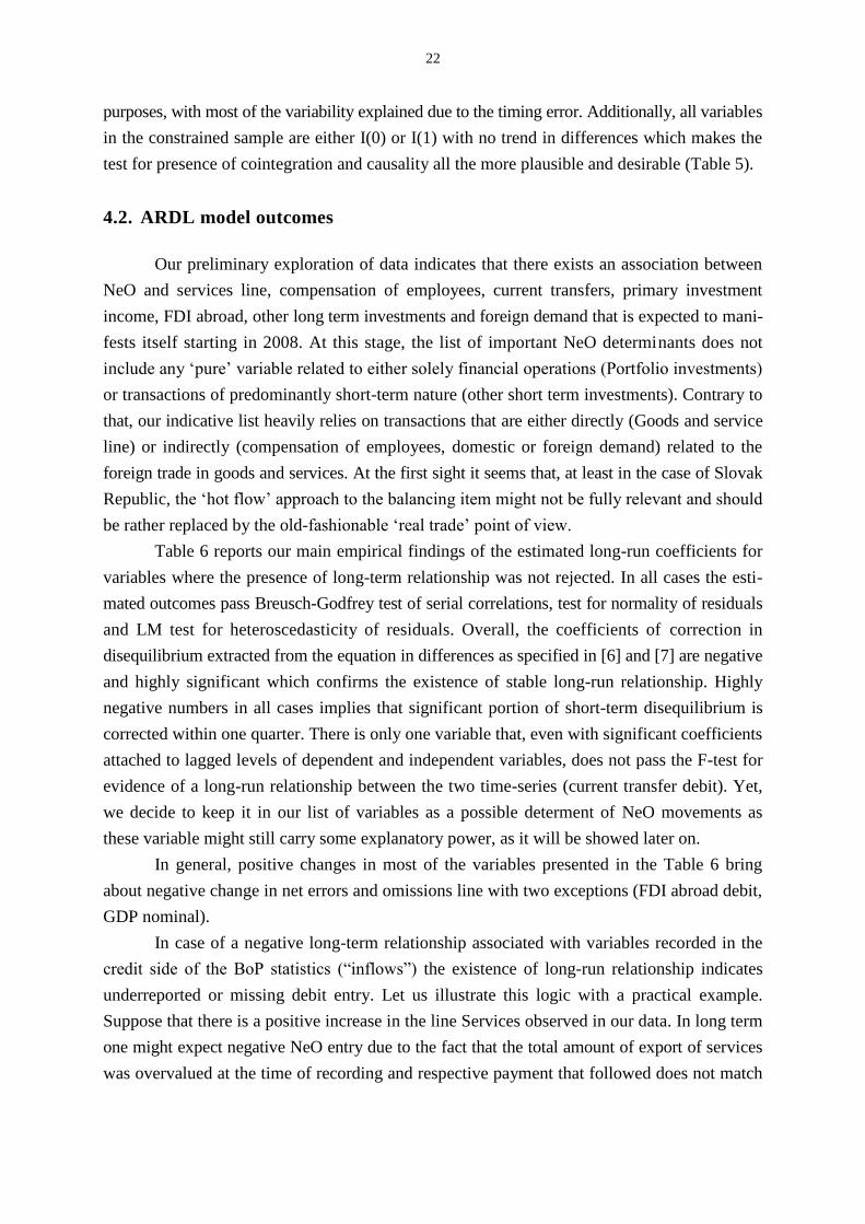
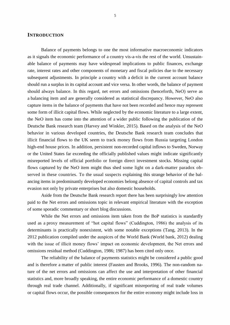
22

purposes, with most of the variability explained due to the timing error. Additionally, all variables

in the constrained sample are either I(0) or I(1) with no trend in differences which makes the

test for presence of cointegration and causality all the more plausible and desirable (Table 5).

4.2. ARDL model outcomes

Our preliminary exploration of data indicates that there exists an association between

NeO and services line, compensation of employees, current transfers, primary investment

income, FDI abroad, other long term investments and foreign demand that is expected to mani-

fests itself starting in 2008. At this stage, the list of important NeO determinants does not

include any ‘pure’ variable related to either solely financial operations (Portfolio investments)

or transactions of predominantly short-term nature (other short term investments). Contrary to

that, our indicative list heavily relies on transactions that are either directly (Goods and service

line) or indirectly (compensation of employees, domestic or foreign demand) related to the

foreign trade in goods and services. At the first sight it seems that, at least in the case of Slovak

Republic, the ‘hot flow’ approach to the balancing item might not be fully relevant and should

be rather replaced by the old-fashionable ‘real trade’ point of view.

Table 6 reports our main empirical findings of the estimated long-run coefficients for

variables where the presence of long-term relationship was not rejected. In all cases the esti-

mated outcomes pass Breusch-Godfrey test of serial correlations, test for normality of residuals

and LM test for heteroscedasticity of residuals. Overall, the coefficients of correction in

disequilibrium extracted from the equation in differences as specified in [6] and [7] are negative

and highly significant which confirms the existence of stable long-run relationship. Highly

negative numbers in all cases implies that significant portion of short-term disequilibrium is

corrected within one quarter. There is only one variable that, even with significant coefficients

attached to lagged levels of dependent and independent variables, does not pass the F-test for

evidence of a long-run relationship between the two time-series (current transfer debit). Yet,

we decide to keep it in our list of variables as a possible determent of NeO movements as

these variable might still carry some explanatory power, as it will be showed later on.

In general, positive changes in most of the variables presented in the Table 6 bring

about negative change in net errors and omissions line with two exceptions (FDI abroad debit,

GDP nominal).

In case of a negative long-term relationship associated with variables recorded in the

credit side of the BoP statistics (“inflows”) the existence of long-run relationship indicates

underreported or missing debit entry. Let us illustrate this logic with a practical example.

Suppose that there is a positive increase in the line Services observed in our data. In long term

one might expect negative NeO entry due to the fact that the total amount of export of services

was overvalued at the time of recording and respective payment that followed does not match

23

the credit entry value. Thus, because of the differences in valuation due to various economic rea-

sons overvalued exports goes hand in hand with underreported foreign assets.

Positive change in the variables recorded in the debit side of the BoP statistics coupled

with negative expected change in the NeO item tells a different story. If there is an increase in

import of services (debit record) the value of the underlying payment (credit) must exceed the

officially invoiced value of import in order to induce negative entry in the NeO line.

Variables capturing change in the domestic or foreign demand for imported or exported

goods, respectively, may have a different impact on the NeO behavior. Negative relationship

between domestic demand (nominal GDP) and NeO series links increasing domestic demand

to undervaluation of import with trade in either goods or services. On the other hand, positive

impact of change in foreign demand for domestically produced goods or services translates

into positive increase of NeO item in the case of undervalued export, i.e. lower amount of

money transferred as a payment than officially invoiced volume of trade.

One serious problem with all equations presented in the Table 6 is related to the omitted

variable bias. From this reason we take those variables that show promising evidence of sig-

nificant long-term causal relationship in bivariate regression and combine them into set of

models that are expected to achieve highest predictive power of the NeO movement in the post

2008 period. Results from the estimations in levels based on Engle-Granger two-step cointegra-

tion approach are presented in the Table 7.

As expected, a relatively high correlation among set of explanatory variables precludes

us from entering all suspects into one regression. Thus, we include and exclude variables

step-wisely based on the underlying correlation matrix. In that sense, we combine export-related

variables (Goods credit, Services credit, foreign demand) with import-related variables

(Goods debit, Services debit, domestic demand) but never pick up two variables belonging to

the same group.

T a b l e 5

ADF unit root tests

ADF unit root test

1997q1-2014q2 2008q3-2014q2 In levels

(constant) In levels

(constant. trend)

First differences (constant)

First differences (constant, trend)

I(d) In levels (constant)

In levels (constant.

trend)

First differences (constant)

I(d)

NeO 0.8274 0.7142 0.0000*** I(1) 0.4465 0.7230 0.0000*** I(1) Goods credit 0.9666 0.4426 0.0004*** I(1) 0.9427 0.0328 0.0361** I(1) Goods debit 0.9481 0.2591 0.0001*** I(1) 0.9483 0.0606 0.0292** I(1) Services credit (logs) 0.8903 0.6619 0.0297** I(1) 0.7788' 0.8373' 0.0003*** I(1) Services debit (logs) 0.8633 0.6622 0.0282** I(1) 0.5747' 0.9720' 0.0018*** I(1) Income – Comp. employees credit 0.9486 0.5464 0.1681 0.4488 I(2) 0.9596 0.8564 0.0000*** I(1) Income – Comp. employees debit (2008q2) 0.9402 0.5341 0.0000*** I(1) 0.8714 0.8780 0.0000*** I(1) Income – Investments credit 0.8756 0.7717 0.0000*** I(1) 0.3043 0.9751 0.0004*** I(1) Income – Investments debit (2008q4) 0.8056 0.4828 0.0000*** I(1) 0.4421 0.6889 0.0276** I(1) Current transfers credit 0.6739 0.9440 0.0000*** I(1) 0.5795 0.6032 0.0000*** I(1) Current transfers debit (logs) 0.8587' 0.7180' 0.0374** I(1) 0.1320 0.8987 0.0000*** I(1) FDI abroad credit 0.8300 0.0000*** 0.0000*** I(1) 0.0013*** I(0) FDI abroad debit 0.7043 0.9871 0.0000*** I(1) 0.8654 0.9870 0.0000*** I(1) FDI in reporting economy credit 0.9302 0.6409 0.0076*** I(1) 0.3586 0.2099 0.0001*** I(1) FDI in reporting economy debit 0.9336 0.6431 0.0000*** I(1) 0.2188 0.4182 0.0016*** I(1) Portfolio investments credit 0.3591 0.9571 0.0000*** I(1) 0.8713 0.5043 0.0000*** I(1) Portfolio investments debit (2008q4) 0.4887 0.9676 0.0000*** I(1) 0.7384 0.7568 0.0421** I(1) Other investments long term credit 0.5118 0.3137 0.0001*** I(1) 0.7868 0.3046 0.0015*** I(1) Other investments long term debit 0.4925 0.2038 0.0000*** I(1) 0.8762 0.7994 0.0019*** I(1) Other investments short term credit 0.7878 0.8367 0.0297** I(1) 0.1850 0.3015 0.0000*** I(1) Other investments short term debit 0.7856 0.8377 0.0000*** I(1) 0.1017 0.3301 0.0000*** I(1) Export factor (2008q1) 0.3437 0.6129 0.0734* I(1) 0.7614 0.9377 0.0058*** I(1) Import factor 0.8741 0.0184** 0.0000*** I(1) 0.8718 0.4079 0.0015** I(1) GDP nominal 0.9439 0.6579 0.2858 0.6151 I(2) 0.8935 0.3566 0.0000*** I(1) GDP real 0.9073 0.6789 0.3173 0.6533 I(2) 0.0375** I(0) GDP world nominal (2009q1) 0.8532 0.6041 0.0225** I(1) 0.9460 0.3665 0.0008*** I(1) GDP world real 0.5862 0.7020 0.0276** I(1) 0.9298 0.4141 0.0001*** I(1)

Note: ADF test is used for test of stationary of time series variables, i.e. H0 assumes that series are non-stationary. Lags of dependent variable used to obtain white-noise

residuals are determined using modified Akaike Information Criterion (MAIC) and modified Bayesian Information Criterion (MBIC). As discussed in Ng and Perron (2001) in

case of the severity of size distortions modified AIC and BIC proposed in their paper are preferred. ‘ bold highlighted series denote series in logs. Time in the brackets denotes

starting quarter of the period tested within the subsample of 1997q1-2014q2 sample; all variables without time specified in the bracket are tested on 2008q3-2014q2 period.

T a b l e 6

ARDL bounds test model outcomes

First difference of

NeO as dependent

variable

Goods credit Goods debit Services

credit

Services

debit

Income –

employees

credit

Current

transfers

debit

FDI abroad

debit

Other investments

LT credit

Other investments

LT debit

GDP nominal

GDP world

nominal

Lag 2 2 1 1 1 2 1 1 1 1 2

const 1 779*** 1 609*** 29 105*** 20 102 *** 7 178*** 351.4 -3 120.3*** -85.53 -42.47 4 699** 4 192**

(0.0131) (0.0299) (0.0000) (0.0061) (0.0004) (0.4432) (0.0012) (0.7965) (0.8998) (0.0194) (0.0193)

dependent(-1) -0.747** -0.589** -1.417*** -0.979*** -1.713*** -0.674** -1.204*** -0.906*** -0.940*** -0.793*** -0.597***

(0.0118) (0.0288) (0.0000) (0.0003) (0.0000) (0.0415) (0.0097) (0.0004) (0.0002) (0.0005) (0.0011)

independent(-1) -0.128*** -0.114** -4 013*** -2 749*** -17.99** -1.251* 3.403*** -0.186* -0.216** -0.222** 0.000**

(0.0079) (0.0191) (0.0000) (0.0049) (0.0002) (0.0976) (0.0019) (0.0702) (0.0493) (0.0144) (0.0194)

dif_independent(-1) 0.030 0.007 2 107** -693.0 12.94*** 0.814 -2.104*** 0.054 0.099 0.093 0.000

(0.6749) (0.9158) (0.0107) (0.6562) (0.0009) (0.3705) (0.0097) (0.6538) (0.3665) (0.1954) (0.9755)

dif_independent(-2) 0.089* 7.50** -1.392*** 0.000

(0.0996) (0.0355) (0.0015) (0.5559)

dif_dependent(-1) -0.344* -0.478** 0.048 -0.059 0.171 -0.372 -0.024 -0.143 -0.137 -0.248 -0.500***

(0.0764) (0.0183) (0.7499) (0.7547) (0.3018) (0.2772) (0.9169) (0.5397) (0.5576) (0.1695) (0.0000)

dif_dependent(-2) -0.276 -0.303* -0.239 -0.197

(0.1161) (0.0918) (0.1785) (0.2157)

Autocorrelation test (0.928) (0.800) (0.308) (0.367) (0.905) (0.221) (0.825) (0.600) (0.785) (0.723) (0.737)

Normality of residuals (0.454) (0.377) (0.494) (0.696) (0.577) (0.386) (0.887) (0.204) (0.197) (0.188) (0.177)

Heteroscedasticity test (0.298) (0.252) (0.605) (0.432) (0.852) (0.504) (0.348) (0.662) (0.474) (0.669) (0.240)

F-test statistics 6.427** 5.409* 30.71*** 9.915*** 31.28*** 2.822 10.40*** 10.50*** 11.43*** 9.390*** 9.126***

Long run multiplier -0.171 -0.195 -2 831 -2 808 -10.50 -1.856 2.826 -0.206 -0.230 -0.280 0.000

Correction in -0.6298 -0.5748 -1.5348 -1.0354 -1.4989 -0.6340 -0.7328 -0.7792 -0.8204 -0.7558 -0.5457

disequilibrium (0.019) (0.032) (0.000) (0.000) (0.000) (0.052) (0.009) (0.003) (0.002) (0.003) (0.008)

Note: ARDL bound test performed, lags specified according to the BIC information criteria from VAR system and adjusted for no autocorrelation present and normality of

residuals. Standard errors estimated with heteroscedasticity robust standard estimator. Values in brackets represent respective p-values. Autocorrelation test by Breusch-Godfrey

test for autocorrelation up to order 4, normality of residuals tested by Jarque-Berra test, heteroscedasticity of residuals tested by White’s test for heteroscedasticity, joint H0

hypothesis of long run coefficients equal to zero tested by F-test. Critical values for F-test for joint H0 hypothesis for lower and upper bound taken from Narayan (2003) are

(8.1700, 9.2850), (5.3950, 6.3500) and (4.2900, 5.0800) at 1%, 5% and 10% significance level, respectively. Engle-Granger cointegration procedure used to extract long run

coefficients from model in levels, ADF unit-root test applied on residuals from Engle-Granger cointegration equation in levels with critical values taken from MacKinnon

(1996). Number of lags in ADF test for dependent variable specified by modified Akaike Information Criterion (AIC). Coefficients of correction in disequilibrium calculated

from equations in differences with residuals extracted from Engle-Granger cointegration equation in levels. Grey-highlighted variables are predicted to have a positive long-run

relationship with the NeO item.

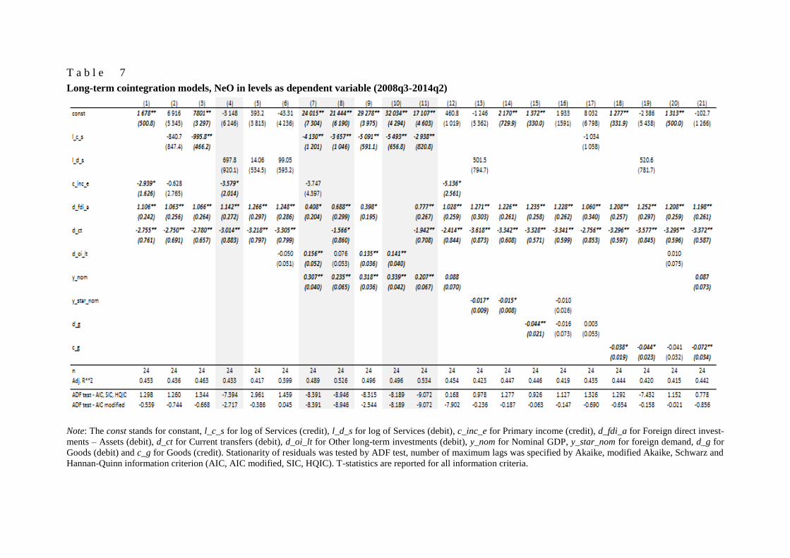
T a b l e 7

Long-term cointegration models, NeO in levels as dependent variable (2008q3-2014q2)

Note: The const stands for constant, l_c_s for log of Services (credit), l_d_s for log of Services (debit), c_inc_e for Primary income (credit), d_fdi_a for Foreign direct invest-

ments – Assets (debit), d_ct for Current transfers (debit), d_oi_lt for Other long-term investments (debit), y_nom for Nominal GDP, y_star_nom for foreign demand, d_g for

Goods (debit) and c_g for Goods (credit). Stationarity of residuals was tested by ADF test, number of maximum lags was specified by Akaike, modified Akaike, Schwarz and

Hannan-Quinn information criterion (AIC, AIC modified, SIC, HQIC). T-statistics are reported for all information criteria.

27

Additionally, some of the variables are strongly related to each other due to the possible

presence of a third lurking variable that influences both of them. An eminent example of this

spurious relationship links ‘Compensation of employees’ credit item with export-related va-

riables (goods credit, services credit). Both the ‘Compensation of employees’ credit item and

export of goods or services are likely to strongly respond to changes in foreign demand. In

other words, growth of foreign demand is likely to affect ‘Compensation of employees’ line

in two ways: a) there is a higher probability of positive increase in the number of people season-

ally working abroad, b) nominal wages earned abroad are expected to follow this positive

shock. Altogether, positive trend in foreign demand boosts both domestic export as well as

money inflows captured by the ‘Compensation of employees’ credit item.

We start our estimation algorithm with four variables for which two tests (Bai-Perron,

Quandt-Andrews) indicated break in possible cointegration relationship in second or third

quarter of 2008, namely Services (credit) with Services (debit) as an alternation, Compensa-

tion of employees (credit), Current transfer (debit), FDI abroad (debit), and alternate among

various combinations to control for possible spurious relationship (models [1]-[5] in Table 7).

In all of the cases current transfers and FDI remain highly significant with negative sign. As

discussed, trade in services is likely to be correlated with ‘Compensation of employees’ item

which is illustrated in the model [2] when both variables lose their explanatory power once

jointly included into regression.

In all of the cases examined, import of services does not prove to be statistically

significant once controlling for other possible NeO determinants (models [4]-[6], [13] and

[19]). However, initially negative response from import of services to NeO item turns out to

become positive in the multiple regressions indicating that part of the import in services might

be in reality over-reported, i.e. consecutive monetary transfer is of lower value that the

invoice value. Contrary to that, export of services enters all equations with negative coefficients

and is significant in majority of cases. Comparing the magnitude of average response of NeO

to both determinants leads to a tentative conclusion that while both variables might suffer

from over-recording issue the primary cause of missing foreign assets should be sought for in

the export side of the trade in services.

Turning eyes into multiple regressions, switch of signs occurs in two other cases, as

well. Domestic demand included in the models [7]-[12] happens to enter regression with positive

signs and all the time statistically significant. Again as in the case of import of either goods or

services, positive change in the domestic demand is about to bring positive change in the NeO

series which indicates possible over-reporting in the debit side of the BoP. Contrary to that,

positive change in foreign demand for domestically produced goods and services (models

[13], [14], [16] and [23]) implies negative development in the NeO pointing out towards over-re-

ported exports not matching their respective settlement values in monetary terms.

Trade in goods might be viewed as a substitute variable for export and import of services

as far as the multiple regression analysis is concerned. Export of goods enters all equations

28

([18]-[21]) with a negative sign and is predominantly statistically significant. Import of goods

proves to be significant in only one case (equation [15]) but loses its explanatory power once

coupled with other export-associated determinants (foreign demand or export of services).

Overall, trade in goods reflects a more general trend embedded in many other variables affecting

the NeO evolution since 2008 but the response of the balancing item to the trade in goods is

weaker than in some other cases.

Second group of models presented in the equations [6] to [10] incorporates the only

“pure” financial transactions from the Balance of Payments (other long-term investments)

meeting the “hot money flow” concept criteria that survives our elimination procedure. As

a high correlation between credit and debit side of the other long-term investment account

(0.97) makes choice between two sides of one account nonessential we keep debit side of this

item due to its relatively higher statistical significance (Table 7). From the conceptual point of

view, as the NeO should to some extent reflect capital flight, debit side of the other long-term

investment account seems to be a more natural choice for our estimations. Positive sign

attached to debit side of the ‘Other long-term investments’ account suggests that the entry in

credit side of a non-specified corresponding account is of a lower value driving balancing

item into positive numbers.

Using the standard Engle-Granger procedure we test the residuals for stationarity by

the ADF test with standard and modified information criteria. Only five models ([4], [7], [8],

[10], [11]) might be considered to capture a joint cointegration relationship among underlying

determinants and the balancing item, as apparent from the Table 7. Three models that are chosen

to best fit NeO evolution in the 2008+ period are [4], [10] and [11]. Model [4] incorporates

inflow of capital in from of income of employees as an important explanatory variable. Two

other includes export of services and domestic demand variables but differ in inclusion of

long-term other investments in the former and foreign direct assets and current transfers accounts

in the latter case. Both models belong to a group with highest explanatory power measured by

adjusted R^2, as well.

29

5. FOUR STORIES BEHIND THE TRENDING BALANCING ITEM

A purely statistical and econometrical exploration of the relationship between balancing

item and various economic variables is of no value if not given a fitting economic story. In this

section we discuss four possible scenarios that would possibly illuminate dark matter hidden

in the non-reported parts of the balance of payments statistics.

5.1. Foreign trade in goods and services

All empirical evidence presented in this article leads us to believe, that significant portion

of the balancing item behavior is driven by real trade in services, followed by trade with

goods. Three poignant issues comes immediately into mind while discussing illicit capital

flows – (i) misinvoicing practices, (ii) value effect due to the exchange rate fluctuations and

(iii) change in trade credit delinquency rate (default rate).

Ad (i). Trade misinvoicing is a method used for moving money illicitly across borders

by misreporting value of a commercial transaction on an invoice submitted to customs (Span-

jers and Foss, 2015). In general, there are three reasons for moving money abroad through

misinvoicing practices: (i) money laundering, (ii) capital control avoidance, (iii) tax purposes.

Balancing item will capture misreporting practices only in such a case if there exists a differ-

ence between invoice value and the subsequent money transfer. This case usually involves ex-

istence of a third middle-men party residing in offshore center that is in charge of issuing an

invoice on behalf of the exporter (importer). Payment for export (import) of goods or services

is only partially credited to the domestic bank account with the rest of the payment transferred

to the offshore bank account owned by domestic exporter and vice versa. If the change in for-

eign assets is not reported to officials the difference will fall into the NeO category.

Our estimations do not lead to any evidence of possible misinvoicing practices in trade

with goods in either export or import side for post 2008 period respecting the standard procedure

for estimating the level of trade misinvoicing (e.g. Kar and Freitas, 2013). Trade in services

should become a subject of a deeper scrutiny; however, as all our evidence suggests that the

adverse behavior of the NeO is to be, at least partially, attributed to the cross-border trade in

services. Unfortunately, up to this date there does not exist any official database summarizing

bidirectional trade in services (such as DOTS compiled by the IMF) on individual country

level, a fact that does preclude us from commenting on any possible role of misinvoicing

practices of the balancing item behavior in the post 2008 period.

The importance of reliable statistics on trade in services has been widely acknowledged.

According to the regulation adopted by the National Bank of Slovakia in 2013 the quarterly

report on foreign services received and provided is to be submitted by all non-banking corporate

30

subjects and foreign affiliates located in the Slovak Republic. Threshold value for reported

transactions is EUR 500. This strict regulation follows list of international documents including

ECB’s recommendation (ECB/2011/24), 6th edition of the BoP Manual by IMF, Commission

regulation (EU) No 555/2012 amending Regulation (EC) No 184/2005 of the European

Parliament and of the Council on Community statistics concerning balance of payments,

international trade in services and foreign direct investment and 2010 Manual on statistics of

international trade in services by OECD. Yet, even with the most accurate statistics on trade

with services available, if part of monetary payment is being charged on domestically owned

foreign account not reported to official authorities, underestimation of level of foreign assets

will remain a pressing issue.

Ad (ii). Decision regarding the currency denomination in foreign trade is an important

one and as such has been subject to various studies (e.g. Reiss, D. G., 2015). If export or im-

port is denominated in domestic currency, any costs related to exchange rate fluctuations will

be borne by the counterparty with no effect on the subsequent monetary payment recorded in

the domestic balance of payments statistics. A completely different story unfolds once low

bargaining power of domestic exporters and importers force them to accept counterparty’s or

third party currency (USD or EUR predominantly) as an invoice currency. In this case,

exchange rate fluctuations will be directly transmitted into the NeO balancing item due to the

difference between invoiced value and subsequent monetary payment.11

With the euro adoption in 2009 the direct exchange rate costs for Slovak businesses

have been substantially diminished. Yet, with 62 (56) percent of Slovak export and 59 (59)

percent of Slovak import in services (goods) in 2013 transported outside the EA jurisdiction,

possible exchange rate costs borne by Slovak businesses may still represent a relatively strong

factor introducing possible disturbances into the balance of payments statistics. Nevertheless,

according to the ECB statistics (ECB, 2014), the euro’s share as an invoicing/settlement

currency12

in extra-euro trade in goods-related transactions approaches 96 percent of total

export and 67 percent of total import value in 2013.13

In other words, while the export side

should be free of exchange rate risk, 1/3 of import might still be subject to major exchange

rate fluctuations.14

In case of services for which no data are available this portion might approach

even bigger numbers. Relate this facts to empirical results, debit side of Services or Goods

11

This reasoning assumes that the exchange rate is market-determined, i.e. domestic economy operates in free or

manageable floating exchange regime. In case of a fixed exchange rate against major trade partner, balancing

item should not be affected. 12

For purpose of this paper we do not distinguish between invoice and settlement currency. It has been consistently

reported in the literature that the invoice currency usually does not differ from settlement currency used in payment

for exported or imported goods or services (e.g. Friberg and Wilander, 2008). However, is some circumstances

this might not always hold true (Reiss, 2015). 13

Data for Slovakia are available only for trade with goods. 14

Even without more detailed statistics, it is reasonable to assume that the 1/3 of import denominated in other

than EUR currency comes predominantly from import of raw materials and commodities usually denominated in

US dollars. In Slovak case, almost one hundred percent of oil import is denominated in US dollars (ECB, 2015).

31

item might not only introduce short-term turbulences into the NeO but may translate into negative

long-term trend in case of continuing domestic currency depreciation.

Ad (iii). As the financial crisis had been enfolding drop in world trade surpassed any

expectations based on the standard modelling techniques. Unproportioned contraction in

world trade in magnitude of 12.2 percent compared to drop in world GDP of 0.6 has led

researchers to name this phenomenon ‘The Great Trade Collapse’. In the Slovak case, while

drop in nominal GDP averaged 3.5 percent, trade with goods contracted by 5.5 percent and

trade with services by 2.5 percent in 2009. Demand-side explanations have been focusing on

drop in overall demand for imported goods, yet has not been able fully explain far higher re-

sponse in world trade than predicted. Supply-side causes include trade financing issues and

breakdown of supply chains.

Trade credit refers to external form of financing that companies receive from their

business partners in form of delayed payment for delivery of services or goods. Inter-firm

trade credit represents the second most significant source of overall external financing after

bank debt (e.g. Petersen and Rajan, 1997). Even though the dominant view in empirical litera-

ture places trade credit alongside with bank debt as substitutes, Bastos and Pindado (2012) show

that economic of financial crisis might change the relationship into complementary one be-

cause of possible contagion.

There are three possible channels through which change in inter-firm trade credit

conditions may affect NeO behavior: (i) increase in the bankruptcy levels in either domestic

exporting firms or foreign importers leads to BoP inconsistency as the monetary payments

linked to real transfer of goods or services are not recorded because of the counterparty’s

default on trade credit; (ii) trade credit rescheduling through extended maturity introduces

higher variability of the NeO series due to the timing error; (iii) overall contraction (complements)

or expansion (substitutes) in trade credit volume as a response to tightened bank lending

conditions may positively, or negatively in latter case, affect balancing item volatility due to

the timing error. In general, overall impact on the NeO series behavior might target both the

series variability (timing error) and stability (introducing negative trend into NeO series as

trade credit defaults spread widely over domestic or foreign economy).

OECD data on number of entrepreneurship bankruptcies for set of developed countries

show overall increase starting in 2009 and culminating in 2010 for most of the economies.

The same pattern is applicable on the Slovak economic conditions. With no empirical evidence

available in our hands related to the default rate on trade credit or extent of trade credit re-

scheduling in foreign trade with goods and, predominantly, services our results should rather

serve as a possible hint leading this direction. Increased volatility in NeO series coupled with

contraction in overall trade in services and goods in the post 2008 period would indicate rise

in timing error in the series pointing out to possible maturity transformation in trade credit.

Negative trend in NeO series might be induced by steady grow in both bankruptcy levels

among foreign trade partners or domestic exporting firms.

32

5.1.1. Cross-border vs. national concept in trade statistics

As pointed out in the report by National bank of Slovakia (2015), negative evolution

of the balancing item might be partially attributed to the conceptual change in recording of

trade with goods. Shift from traditionally used cross-border to national concept of recording

decreased absolute value of balancing item in more than 50 percent in years 2010 and 2011.

However, even after accounting for this phenomenon negative evolution of the Slovak’ balancing

item remains taunting. Further discussion on possible link between mis-invoicing practices,

change in reporting concepts and NeO evolution is presented in the Appendix 2.

5.2. Cross-border and seasonal work and economic crisis

Slovakia, as well as other transition countries, had experienced a continual increase in

the number of seasonal and temporary cross-border workers before the year 2008 that might

have been attributed to the opening up of European labor market, among other factors. Economic

crisis transmitted into highly exposed Slovak economy in 2009 had reversed this positive

trend and led to severe drop in (in)official numbers of workers employed abroad (Kahanec

and Mytna Kurekova, 2014) as well as to overall decrease in their net earnings.

In general, there are four accounts in the balance of payments statistics that should be

jointly affected due to this negative phenomenon – Services (Debit side), Primary income

(Compensation of employees), Secondary income (Social contributions) and Other investments

account. Gross earnings from work abroad are recorded in the credit side of the Compensation

of employees with respective charges for social contribution in Secondary income debit side

(IMF, guideline, p. 53). Estimated amount of cross-border workers expenditures associated

with daily living costs are recorded as import of services under the Travel sub-account. Net

earnings, either wired through bank transfer or shipped in physical form to domestic economy

increase holdings of foreign assets in the debit side of the financial account. As discussed

previously, both credit side of the compensation of employees and debit side of the current

transfers (secondary income) belong to the group of potential suspects causing the negative

trend in the balancing item (Table 6 and Table 7). Additionally, import of services enters our

models as one of the potentially important explanatory variable, based on the ARDL bound

test estimation outcomes.

Estimating the level of remittances and, to some extent, of compensation of employees

is a very difficult job, indeed. Usually, central banks and statistical offices present conservative

estimates extrapolated from various empirical models. As a result, the chances are that incon-

sistency between officially estimated and reported values of remittances and real flow of

money transferred through banking sector (capital inflow via bank deposits recorded in Other

investments category; physical conversion of foreign currency) or outside of it (shadow

banking, black market with foreign exchange, informal channels) will be significant. The sec-

ond case might not be even fully captured by the BoP statistics if shadow banking and foreign

33

exchange markets are present, assumption which is almost for sure satisfied in case of many

developing countries operating various forms of fixed exchange rate regimes. Informal chan-

nels refuse to be even accounted for especially in a common monetary union characterized by

impossibility to distinguish country of origin of a currency.

Part of the inconsistency reflected in the NeO numbers will be present due to the

“omitted” transactions principle.15

As an immediate consequence, BoP data are likely to fail

to capture transfers in low-income group of citizens (migrants) who, predominately, are those

who are making a one big bulk of all transactions in remittances.

One of the possible stories partially explaining the ongoing negative trend in the NeO

item thus connects drop in cross-border permanent and seasonal work as a result of the overall

adverse economic conditions with failure to capture ‘true’ extent of money transfers between

Slovak residents and foreign economic entities. Assuming that the underlying model employed

by the National Bank of Slovakia in cooperation with the Statistical office of the Slovak

Republic for estimating the value for compensation of employees is an accurate one, the

opposite relationship captured by the negative sing in the econometric estimations would imply

that increasing part of the money transfers is not accounted for, thus effectively underestimating

level of foreign assets held by domestic households abroad. However, questioning the predic-

tive power of the model, as we are more inclined to do, might lead to a conclusion that the

inaccuracy spotted comes rather from the overestimated level of compensation of employees

recorded in the current account. Thus, the foreign assets value is to be unaffected whilst current

account balance should be rather scaled down.

5.3. Foreign direct investments abroad

Among the statistically significant variables linked to the balancing item with long-term

cointegration relationship one stands out. Capital outflow recorded in the ‘Foreign direct

investments abroad’ account relates directly to the issue of missing foreign assets in interna-

tional investments position statistics.

In general, there exist specific cases when the inflow or outflow of FDI might not be

properly measured and will cause disturbances in BoP, therefore affecting the NeO item as

a consequence. First group of transactions would be inherently linked to problems of reporting

and cannot be interpreted as illicit. All intracompany lending might be a source of disturbances

in the NeO position, if not properly accounted for, meaning that underlying financial flow

takes place (reported in the bank statistics) but information about the intercompany lending is

not provided and foreign direct investment account is not credited or debited appropriately.

Same holds for retained earnings category. In general, any movement of goods, services or

capital between affiliated enterprises might become a source of disturbances if not properly

15

For example, any transfer made between Euro area residents and outsiders that is below the threshold value of

EUR 12,500 is not recorded at all.

34

identified. For a further reference, the Table 8 presents possible combinations between NeO

item and various transactions.16

T a b l e 8

FDI-related intercompany transactions and impact on Net errors and omissions account

Credit Debit NeO

Shipment of goods between affiliates without

payment

No payments, failing to recognize as a FDI transaction

Negative

No payments, failing to recognize as a FDI transaction

Shipment of goods between affiliates without

payment

Positive

Provision of services among affiliates (consul-

tancy, marketing, know-how)

No payments, failing to recognize as a FDI transaction

Negative

No payments, failing to recognize as a FDI transaction

Provision of services among affiliates (consultancy,

marketing, know-how)

Positive

Shipment of goods between affiliates Provision

of services among affiliates (consultancy, mar-

keting, know-how) with payment

Recognized as a FDI transaction, Payment in bank statistics

Positive

Recognized as a FDI transaction, Payment in bank statistics

Shipment of goods between affiliates Provision

of services among affiliates (consultancy, mar-

keting, know-how) with payment

Negative

Intercompany lending – loan to affiliated com-

pany paid recorded in bank statistics

Missing entry in the FDI item Negative

Missing entry in the FDI item Intercompany lending – loan from affiliated

company received recorded in bank statistics

Positive

Let us turn our attention to FDI done by private individuals (household) in form of

stocks or shares. It has been relatively recently recognized that while data on standard FDI

conducted by non-financial corporations are usually well documented as they stand in the

center of public’s attention, foreign direct investments made by private citizens is likely to

remain outside of official recording systems (Blomberg, Forss and Karlsson, 2003) even

though the official reporting requirements exist.

Problem with the FDI of individuals is that only one side of the transaction is captured

(bank transfer) but no accommodating transaction can be identified (FDI, portfolio or other

16

Since seminal paper by Hausmann and Sturzenegger (2007) it has been acknowledged that foreign assets of

countries might be hugely understated due to the role of unrecorded intangible capital (patents, know-how, reputation,

marketing expertise etc.). So what is the relationship between dark matter elements and net errors and omissions

in the balance of payments? First of all, huge part of the dark matter elements as described by Hausmann and

Sturzenegger (2007) will not be captured in the balance of payments statistics at all, thus the NeO line will not be

able to say anything about this issue. Data on transfers of intangible assets between affiliates without respective

payment, even though officially subject to balance of payments reporting, are difficult to collect, measure, record

and report, thus are naturally left outside of the statistics. Secondly, all transactions accompanied with the

respective payments (patents, know-how, marketing, professional education, consultancy services etc.) between

affiliates will not fall into the net errors and omissions category at all if they are not recognized as a foreign direct

investments. In this case the dark matter materializes because transactions between affiliates were not recognized

and were simply recorded as a pure export or import transactions in the current account. If transactions between

affiliated parties are recognized as a foreign direct investment and the respective payment has been made balance

of payments statistic will suffer from double accounting of one leg of transaction, thus the net errors and omissions

will be affected. But in this third case the dark matter would disappear. Only in the case, if those transfers are not

accompanied by the underlying money flow we will be able to observe impact on net errors and omissions category

but we cannot distinguish these transactions from pure exports or imports.

35

investments).17

Problems with portfolio investments become even more severe as both,

households and non-financial companies’ portfolio investments might be missing in the officially

complied statistics.18

Stocks or bonds obtained through a financial intermediary are recorded

unilaterally at the time when the payment is made but the corresponding account will be missing

(specification of transactions).

Now the question stands whether assets or liabilities are more prone to be missing

from the official statistics. In case of non-financial corporations or households for official au-

thority it is basically not possible to collect information about holdings of foreign assets with-

out imposing reporting obligation on these subjects. Additionally, tax optimization possibilities

might motivate domestic investors to hide portion of their wealth from eyes of authorities in

form of foreign assets making officially presented data on foreign assets very misleading, to

say at least.

However, domestically issued securities (liabilities) are possible to track once they are

traded on organized financial markets open to either domestic (no impact on BoP statistics) or

foreign investors (transactions might be included in the BoP statistics). Secondly, banking

statistics might require domestic banks to track separately foreign deposits owned by foreign

citizens.19

In general, one might expect holdings of foreign assets to be significantly underesti-

mated in comparison to level of underestimation of foreign liabilities.20

Possible consequence

17

Suppose a domestic households is about to purchase a stock through a foreign broker. Money is transferred

from a domestic account to the foreign account of a broker in exchange for an ownership rights to a particular

stock. Yet, as the purpose of the transaction was neither recorded nor announced by a domestic household the

banking institution and consequently central bank will not obtain crucial information about the character of this

payment. Only the simple transfer of money from domestic to foreign account is recorded and NeO will fully

absorb missing second leg of this transaction (portfolio investment item from the financial account in this case). 18

Non-bank corporations in Slovakia have an obligation to report to the national bank if their foreign assets or

liabilities exceed value of EUR 2 mil. Officially, every domestic resident (households included) is by law required

to report foreign transactions (bank transfers related to foreign direct investments, loans, securities and operations

on foreign financial markets) to the national central bank. Practically, compliance to this law is hard to estimate.

Up to 2004 every domestic resident needed a permission in order to be allowed to open an account in foreign

bank outside of domestic jurisdiction. With EU accession the permission is not any more required. 19

However, if foreign investor opens a foreign account through middle man who is a resident of that country

than the statistics on foreign liabilities would naturally be distorted. 20

At first sight this reasoning might go against the logic presented in the Coordinated Portfolio Survey conducted

by the IMF. Data presented in this statistics are collected from the asset side and liabilities are derived as a mirror

image to assets for all economies. Some of the countries report also their foreign liabilities (15 countries). However,

the asset position and transaction with them cover only those asset holdings that were made public by their own-

ers. Huge portion of assets (not only) in non-financial corporations or households’ portfolios must be missing in

this statistics. Truly, one might take data for 15 countries that made their estimates of foreign liabilities public to

discover that in 13 cases total reported liabilities are significantly higher than total liabilities derived as a mirror

from reported assets against a particular economy. Average percentage of missing data is 20 percent with Australia

(26 percent) and Japan (40 percent) as a noteworthy exception. While part of this “black hole” might be for sure

attributed to missing data from non-reporting countries this simple exercise shows that if liabilities are tracked,

taking into account all complications with data collection, the picture provided might be much closer to the reality.

One policy recommendation in this case would be then to focus on collection of data for foreign liabilities not

only on the asset side as we see that in some of the reporting countries this exercise is possible and delivers new

insight into the true level of net indebtedness. In Finland, persistent increase in negative cumulative sum of NeO

item pushed the Bank of Finland to reconsider their methodology on compilation of statistics and published

revisions on foreign liabilities that proved to be overestimated at the end, yet work on foreign assets remains

36

of these phenomena is a situation when net level of foreign indebtedness is likely to be

overestimated among many developed but also developing countries.21

T a b l e 9

Portfolio and Other investments-related capital movements and impact on Net errors and omis-

sions account

Credit Debit NeO

Acquiring foreign assets – Bank statistics Missing specification (e.g. PI) Negative

Missing specification (e.g. PI) Selling foreign assets – Bank statistics Positive

Missing specification (e.g. OI) Incurrence of foreign liability – bank statistics Positive

Decrease in foreign liabilities – bank statistics Missing specification (e.g. OI) Negative

Additionally, if capital is being transferred between banking sector (which is subject to

official reporting requirements) and non-bank financial institutions (shadow banking) this

money disappears from other investment items without a respective counter-value. This is one

of key drivers behind the relationship or NeO and speculative money out/inflows. Secondly, if

money are taken out of the bank account (e.g. transformed into bitcoins) and then move out of

a country (cash or in form of digital imprint saved at memory stick) this second-leg of the

movement will not be recorded and the dis-balance will be reflected in the NeO item.

Statistically significant and in all cases positive coefficient associated with the FDI

debit side of the Slovak balance of payments consistently points out to the fact that a change

in FDI entry is accompanied by an un-proportional change (smaller in magnitude but of the

same direction) in associated but not-specified credit entry. In light of the recent study by

Zucman (2015) this outcome might tentatively hint to a presence of tax optimization motives

among Slovak businessmen. As already discussed, intracompany provision of (fictional) ser-

vices among affiliated companies (FDI) might serve as a tool to shift profits to countries with

the most favorable tax environment. With both statistically significant accounts, Services as

well as FDI abroad, part of the NeO evolution might be therefore potentially attributed to this

recent phenomenon.22

theoretical (Salo, 2014). Nevertheless, even after revision substantial negative balance in NeO indicates that

foreign assets underestimation is likely to be blamed. 21

In theory, developed countries are also expected to serve as a source of capital for less developed countries.

Interestingly, savings rate are much higher in developing countries nowadays than in many developed countries,

a fact that could be partially explained by their orientation on export-based growth model, undeveloped financial

markets and low quality of social services. Despite various capital restrictions in place money outflows will

likely to penetrate the barriers through informal channels and grey economy. Thus, missing data on foreign assets

are likely to occur in both developed and developing countries once there are knowledgeable investors present

who are eager to put their money outside of domestic territory due to the various reasons (greed, tax optimization,

unfavorable domestic conditions, wealth expropriation etc.). 22

Quite recently, one of the owners of one Slovak commercial bank commented in social media on their consult-

ing services for their clients belonging to the highest income cohort. Private bankers employed in this bank (but

not exclusively) are said to advise their clients to establish a new business in some of the tax haven countries

(Cyprus, preferably) in order to optimize client’s tax obligations. All the consequent transactions of these clients

should be consequently administered through bank accounts owned by this haven-based shell companies. At the

end, most of the money funds transferred in this way end up being invested in financial assets all around the

globe, yet with minimum to zero effective tax applied on capital gains.

37

5.4. Pure financial speculation and rise of long-term credit

By definition, ‘other investments’ account is a residual category that includes all financial

transactions not recorded in the FDI, portfolio account or reserve assets line. By functional

categorization this item comprises trade credits, loans, currency and deposits, and other assets

and liabilities. In case of the trade credit the item ‘Other investments’ steps up as the second-lag

account coupled with the export or import of goods or services recorded in the current account.

All transactions that include money transfer in either electronic form through bank wire or

payment in cash are recorded in this account.23

Occurrence of significant interconnection between ‘Other investments’ account and

the NeO evolution should not be viewed as a surprising finding. In any of the above discussed

scenario, ‘Other investments’ residual series might be affected as a by-product if the double-

accounting principles link determinant of the NeO evolution (e.g. export of services) with

‘Other investments’ category (e.g. long-term trade credit) because of the character of underlying

transaction. Following this direction of reasoning, the existing link between NeO and 'Other

investments' category does not bear any other added information value except of the fact that

there is a missing piece of information somewhere there in the BoP statistics regarding the

source of the NeO adverse development. Potential suspects may include practically anything

from missing recording on cross-border purchase of domestic government bond, not-reported

acquisition of foreign company shares by domestic private investors to transfer of remittances

between family members scattered across the globe.

The ‘Other investments’ account integrates both short-term transactions that standard-

ly overlap with the ‘hot money’ flow definition and financial transactions of a long-term na-

ture. While in many cases motives driving monetary transactions recorded in this item do not

show signs of speculative behavior, link between short-term ‘Other investments’ item and hot

flow money definition has been widely accepted. From this perspective, a non-existent link

between Slovak NeO evolution and short-term ‘Other investments’ element tentatively suggests

that the NeO behavior in the post 2008 period should be attributed to more fundamental

(=real) factors, such as trade in services or economic migration of labor force, rather than to

speculative incentives so widely cited being the cause of the NeO adverse development.

Long-term component consists from two major contributors. With regard to long-term

trade credit which role has been already discussed, existing relationship between NeO and

23

Banking sector’s transactions were identified by Blomberg, Forss and Karlsson (2003) as one of the four key

factors likely to explain behavior of Swedish net errors and omissions item. Strong connection between banks’

foreign transactions and movements in NeO has been shown particularly in times of higher fluctuations. As

authors point out repeated discussion with banks did not provide any plausible explanation for this phenomenon.

Based on our previous reasoning, we claim that this behavior should not be viewed as a surprising one but rather

as a direct consequence of missing specification of second leg in transactions captured by the banking statistics,

as required by the double-accounting principle. The other investments item as a residual category naturally responds

to any missing information in other accounts of the balance of payments that fall into net errors and omissions

element.

38

long-term component of ‘other investments’ line may provide additional argument in favor

our “real trade” hypothesis in the Slovak case. Second component includes long-term deposits

and bank loans. Own banking sector operations are relatively easily disentangled as banks are

required to report to national authority in a relatively detailed way. It is the operations of clients

(businesses and households) that makes tracking down the purpose and character of a money

transfer so difficult to pin down (Blomberg, Forss and Karlsson, 200; Salo, 2014). Without

a more detailed dataset it is not possible to accept or reject the hypothesis that part of the NeO

adverse behavior is to be contributed to the private non-financial sector foreign operations

whose nature and purpose remains a mystery.

39

CONCLUSION

This working paper fills the literature gap in the empirical analysis regarding net errors

and omissions at least in the context of Central and Easter Europe and with emphasis on

a small and open economy. The paper also sheds some light on the dynamics of net errors and

omissions during the Great Recession and relate the extent to which the findings in this paper

might fit into previous other empirical studies on advanced economies and during relatively

stable time periods. The results seem to suggest the NeO item for Slovakia during the period

under investigation has not been related to illicit financing rather was linked to the real sector

of the economy. Likewise, our estimations do not find any evidence of possible misinvoicing

practices in trade with goods in either export or import side for post 2008 period respecting

the standard procedure for estimating the level of trade misinvoicing. Even though the paper

does not find a phenomenon of illicit financing (hot money flows) during the period under

investigation the link between evolution of foreign direct investments and NeO might provide

evidence of possible tax optimization.

Trade in services should become a subject of a deeper scrutiny, as all our evidence

suggest that the adverse behavior of the NeO is to be, at least partially, attributed to the cross-

border trade in services. Unfortunately, up to this date there is no any official database sum-

marizing bidirectional trade in services (such as DOTS compiled by the IMF) on individual

country level, something that does preclude us from commenting on any possible role of mis-

invoicing practices of the balancing item behavior in the post 2008 period. There is therefore

a call for further research in investigating the link between the service sector and the dynam-

ics of NeO for Slovakia with a more detailed dataset at hand.

40

REFERENCES

ANDREWS, D. W. K. (1993): Tests for parameter instability and structural change with

unknown change point. Econometrica, Vol. 61, No. 4, pp. 821-856.

ANG, J. (2008a): ‘A Survey of Recent Developments in the Literature of Finance and

Growth.’ Journal of Economic Surveys, 22, 536-576.

ANG, J. (2008b): ‘Financial Development and Economic Growth in Malaysia.’ New York:

Routledge.

Australian Bureau of Statistics (1996): Balance of payments statistics: Information paper on

quality. Available at: <http://www.abs.gov.au/Ausstats/abs@.nsf/Lookup/98382A262D7DFD

DFCA25697E0018FDB0?opendocument>.

BAI, J. (1997): Estimating Multiple Breaks One at a Time. Econometric Theory, Vol. 13, No.

3, pp. 315-352.

BAI, J. – PERRON, P. (1998): Estimating and Testing Linear Models with Multiple Structural

Changes. Econometrica 66, pp. 47-78.

BAI, J. – PERRON, P. (2003): Computation and Analysis of Multiple Structural Change Models.

Journal of Applied Econometrics, 18, pp. 1-22.

BASTOS, R. – PINDADO, J. (2013): Trade credit during a financial crisis: A panel data analysis.

Journal of Business Research, Vol. 66, No. 5, pp. 614-620.

BLANKENBURG, S. – KHAN, M. (2012): Governance and Illicit Flows. In Draining Development:

Controlling Flows of Illicit Funds from Developing Countries, ed. Peter Reuter, World Bank.

BLOMBERG, G. – FORSS, L. – KARLSSON, I. (2003): Errors and omissions in the balance of

payments statistics – a problem? Sveriges Riksbank Economic Review, 2003:2, pp. 41-50.

CHOW, G. C. (1960): Tests of Equality between Sets of Coefficients in Two Linear Regressions.

Econometrica 28 (3), pp. 591-605.

COBHAM, A. – JANSKY, P. – PRATS, A. (2014): Estimating Illicit Flows of Capital via Trade

Mispricing: A Forensic Analysis of Data on Switzerland. Working Paper 350, Washington

DC: Center for Global Development.

CUDDINGTON, J. T. (1986): Capital Flight: Estimates, Issues, and Explanations. Princeton

Studies in International Finance, No 58, December 1986.

CUDDINGTON, J. T. (1987): Macroeconomic Determinants of Capital Flight: An Econometric

Investigation. In LESSARD, D. & CUDDINGTON, J. (eds): Capital Flight and Third World Debt,

Washington DC: Institute for International Economics, pp. 85-96.

DOOLEY, M. (1986): Country-specific risk premiums, capital flight and net investment income

payments in selected developing countries. International Monetary Fund, mimeo.

DUFFY, M. – RENTON, A. (1971): An analysis of the U.K. Balancing Item. International Economic

Review, Vol. 12, No. 3, pp. 448-464.

ENGLE, R. F. – GRANGER, C. W. J. (1987): Co-integration and Error correction: Representation,

Estimation, and Testing. Econometrica, Vol. 55, No. 2, pp. 251-276.

European Central Bank (2014): The international role of the euro. Frankfurt am Main: ECB.

41

European Central Bank (2015): The international role of the euro. Frankfurt am Main: ECB.

FAUSTEN, D. K. – BROOKS, R. D. (1996): The balancing item in Australia’s balance of payments

accounts: an impressionistic view. Applied Economics, 28, 1303-1311.

FAUSTEN, D. K. – PICKETT, B. (2004): Errors & Omissions in the Reporting of Australia’s

cross-border transactions. Australian Economic Papers, March 2004, pp. 102-115.

FRIBERG, R. – WILANDER, F. (2008): The currency denomination of exports – a questionnaire

study. Journal of International Economics, 75(1), pp. 54-69.

GUO, D. (2009): Mirror statistics of international trade in manufacturing goods: The case of

China. Research and Statistics Branch Working Paper 19/2009, United Nations Industrial

Development Organization.

HANSEN, B. E. (2001): The New Econometrics of Structural Change: Dating Breaks in U.S.

Labor Productivity. Journal of Economic Perspectives, Vol. 15, No. 4, pp. 117-128.

HARVEY, O. – WINKLER, R. (2015): Dark matter: the hidden capital flows that drive G10

exchange rates. Deutsche Bank Market Research Report, 6 March 2015.

HAUSMANN, R. – STURZENNEGER, F. (2007): The Missing Dark Matter in the Wealth of Nations

and its Implications for Global Imbalances. Economic Policy, Vol. 22, No. 51, pp. 469-518.

HILPINEN, J. (1995): Analysis on the Errors and Omissions in the Finnish Balance of Payments:

Restless Capital Movements, Floating Exchange Rate and Errors Since 1991. Bank of Finland

Discussion Papers 4/95.

INDER, B. (1993): ‘Estimating Long-Run Relationships in Economics: A Comparison of Different

Approaches.’ Journal of Econometrics, 57, 53-68.

International Monetary Fund (1977): Balance of Payments and International Investments

Position Manual, 4th edition. Washington DC: International Monetary Fund.

International Monetary Fund (1993): Balance of Payments and International Investments

Position Manual, 5th edition. Washington DC: International Monetary Fund.

International Monetary Fund (2009): Balance of Payments and International Investments

Position Manual, 6th edition. Washington DC: International Monetary Fund.

International Monetary Fund (2014): BMP6 Compilation Guide. Washington DC: International

Monetary Fund.

KAHANEC, M. – MYTNA KUREKOVA, L. (2014): Did post-enlargement labor mobility help the

EU to adjust during the great recession? The case of Slovakia. CELSI Discussion paper No.

23, Bratislava: CELSI.

KAR, D. – FREITAS, S. (2013): Russia: Illicit Financial Flows and the Role of the Underground

Economy. Global Financial Integrity.

KILIBARDA, B. (2013): Net errors and omissions. Working paper, No. 23. Central bank of

Montenegro.

LANE, P. R. – MILESI-FERRETTI, G. M. (2001): The external wealth of nations: measures of

foreign assets and liabilities for industrial and developing countries. Journal of International

Economics, 55, pp. 263-294.

LIN, M. – WANG, H. (2009): What Causes the Volatility of the Balancing Item? Economics

Bulletin, Vol. 29, No. 4, pp. 2738-2748.

42

MACKINNON, J. (1996): Numerical Distribution Functions for Unit Root and Cointegration

tests. Journal of Applied Econometrics 11, pp. 601-618.

MISHRA, V. – SMYTH, R. – TANG, T. Ch. (2008): Is the balancing item for Australia sustainable?

Evidence from a threshold autoregressive model with an autoregressive unit root. Australian

Economic Papers, June 2008, pp. 190-198.

NARAYAN, P. (2005): ‘The Saving and Investment Nexus in China: Evidence form Cointegration

Tests.’ Applied Economics, 37, 1979-1990.

National Bank of Slovakia (2015): Dopad transakcií nerezidentov na zahraničný obchod

a platobnú bilanciu SR (Impact of transactions of nonresidents on foreign trade and balance of

payment of Slovakia). Commentary. Available at: <http://www.nbs.sk/_img/Documents/_

Statistika/PlatobnaBilancia/Komentar_k_transakciam_nerezidentov_v_ZO.pdf>.

NORDSTOKKE, D. W. – ZUMBO, B. D. (2010): A new nonparametric Levene Test for Equal

Variances. Psicologica, 31, pp. 401-430.

NORDSTOKKE, D. W. et al. (2011): The operating characteristics of the nonparametric Levene

test for equal variances with assessment and evaluation data. Practical Assessment Research

and Evaluation, Vol. 16, No. 5, pp. 1-8.

PEASARAN, M. – SHIN, Y. (1996): Cointegration and Speed of Convergence to Equilibrium.

Journal of Econometrics, 71, 117-143.

PEASARAN, M. – SMITH, R. (1998): ‘Structural Analysis of Cointegration VARs.’ Journal of

Economic Surveys, 12, 471-505.

PEASARAN, M. et al. (2001): ‘Bounds Testing Approaches to the Analysis of Level Relationship.’

Journal of Applied Econometrics, 16, 289-326.

PETERSEN, M. A. – RAJAN, R. G. (1997): Trade credit: Theories and evidence. Review of

Financial Studies, 10, pp. 661-692.

REISS, D. G. (2015): Invoice Currency: puzzling evidence and new questions from Brazil.

Banco Central do Brasil, Working Paper 382, 2015.

SALO, A. (2014): Net errors and omissions of the Finnish balance of payments. Financial

Stability and Statistics, 4/2014.

SPANJERS, J. – FOSS, H. F. (2015): Illicit Financial Flows and Development Indices: 2008-2012.

Global Financial Integrity Report.

TANG, T. C. (2005): Does exchange rate volatility matter for the balancing item of balance of

payments accounts in Japan? An empirical note, RISEC, International Review of Economics

and Business, vol. 52, pp. 581-590.

TANG, T. C. (2006a): The Influences of Economic Openness on Japan’s Balancing Item: An

Empirical Note. Applied Economic Letters, vol. 13, pp. 7-10.

TANG, T. C. (2006b): Japan’s balancing item: Do timing errors matter? Applied Economic

Letters, vol. 13, pp. 81-87.

TANG, T. C. (2007a): Sustainability of balancing item of balance of payments accounts: Fresh

empirical evidence for G7 countries. Applied Economic Letters, vol. 14, pp. 251-254.

TANG, T. C. (2007b): Sustainability of balancing item of balance of payments account for 20

industrial countries. Empirical Economics Letters, 6 (5), 381-388.

43

TANG, T. C. – HOOY, C. W. (2007): The asymmetric and time varying volatility of balancing item

in Australia’s balance of payments. International Journal of Management, vol. 24, pp. 76-81.

TANG, T. C. – LAU, E. (2008): An empirical investigation of sustainability of balancing item

in Asian countries. Applied Economic Letters, vol. 15, pp. 117-123.

TANG, T. C. – LAU, E. (2009): An empirical investigation of sustainability of balancing item

of balance of payment accounts for OIC member countries. Journal of Economic Cooperation

and Development, 30, 1, pp. 1-16.

TANG, T. C. – FAUSTEN, D. K. (2012): Current and capital account interdependence: an empirical

test. International Journal of Business and Society, 13 (3), 229-244.

TANG, T. C. (2013): New perspectives on the ‘Net errors & omissions‘ in balance of payment

accounts: An empirical study – Australia. Monash University Department of Economics

Discussion Paper 54/13.

TOMBAZOS, C. G. (2003): New light on the ‘Impressionistic View‘ of balancing item in

Australia’s balance of payments accounts. Applied Economics, 35(12), pp. 1369-1378.

VUKŠIČ, G. (2009): Croatian balance of payments: implications of net errors and omissions

for economic policy. Institut Za Javne Financije – Newsletter, 41, pp. 1-5.

World Bank (2012): Draining Development: Controlling Flows of Illicit Funds from Developing

Countries, ed. Peter Reuter, Washington DC: World Bank.

ZUCMAN, G. (2015): The Hidden Wealth of Nations: The Scourge of Tax Havens. Longdon:

The University of Chicago Press.

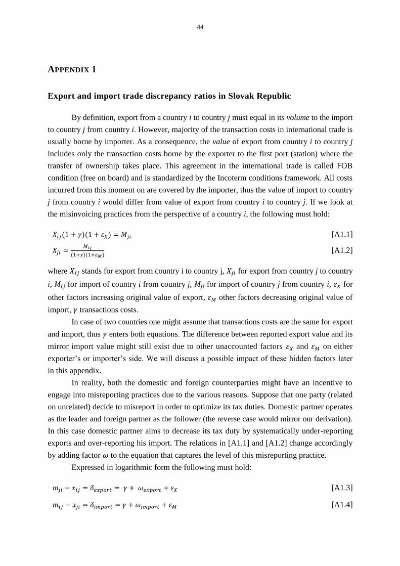
44

APPENDIX 1

Export and import trade discrepancy ratios in Slovak Republic

By definition, export from a country i to country j must equal in its volume to the import

to country j from country i. However, majority of the transaction costs in international trade is

usually borne by importer. As a consequence, the value of export from country i to country j

includes only the transaction costs borne by the exporter to the first port (station) where the

transfer of ownership takes place. This agreement in the international trade is called FOB

condition (free on board) and is standardized by the Incoterm conditions framework. All costs

incurred from this moment on are covered by the importer, thus the value of import to country

j from country i would differ from value of export from country i to country j. If we look at

the misinvoicing practices from the perspective of a country i, the following must hold:

𝑋𝑖𝑗(1 + 𝛾)(1 + 휀𝑋) = 𝑀𝑗𝑖 [A1.1]

𝑋𝑗𝑖 =𝑀𝑖𝑗

(1+𝛾)(1+𝜀𝑀) [A1.2]

where 𝑋𝑖𝑗 stands for export from country i to country j, 𝑋𝑗𝑖 for export from country j to country

i, 𝑀𝑖𝑗 for import of country i from country j, 𝑀𝑗𝑖 for import of country j from country i, 휀𝑋 for

other factors increasing original value of export, 휀𝑀 other factors decreasing original value of

import, 𝛾 transactions costs.

In case of two countries one might assume that transactions costs are the same for export

and import, thus 𝛾 enters both equations. The difference between reported export value and its

mirror import value might still exist due to other unaccounted factors 휀𝑋 and 휀𝑀 on either

exporter’s or importer’s side. We will discuss a possible impact of these hidden factors later

in this appendix.

In reality, both the domestic and foreign counterparties might have an incentive to

engage into misreporting practices due to the various reasons. Suppose that one party (related

on unrelated) decide to misreport in order to optimize its tax duties. Domestic partner operates

as the leader and foreign partner as the follower (the reverse case would mirror our derivation).

In this case domestic partner aims to decrease its tax duty by systematically under-reporting

exports and over-reporting his import. The relations in [A1.1] and [A1.2] change accordingly

by adding factor 𝜔 to the equation that captures the level of this misreporting practice.

Expressed in logarithmic form the following must hold:

𝑚𝑗𝑖 − 𝑥𝑖𝑗 = 𝛿𝑒𝑥𝑝𝑜𝑟𝑡 = 𝛾 + 𝜔𝑒𝑥𝑝𝑜𝑟𝑡 + 휀𝑋 [A1.3]

𝑚𝑖𝑗 − 𝑥𝑗𝑖 = 𝛿𝑖𝑚𝑝𝑜𝑟𝑡 = 𝛾 + 𝜔𝑖𝑚𝑝𝑜𝑟𝑡 + 휀𝑀 [A1.4]

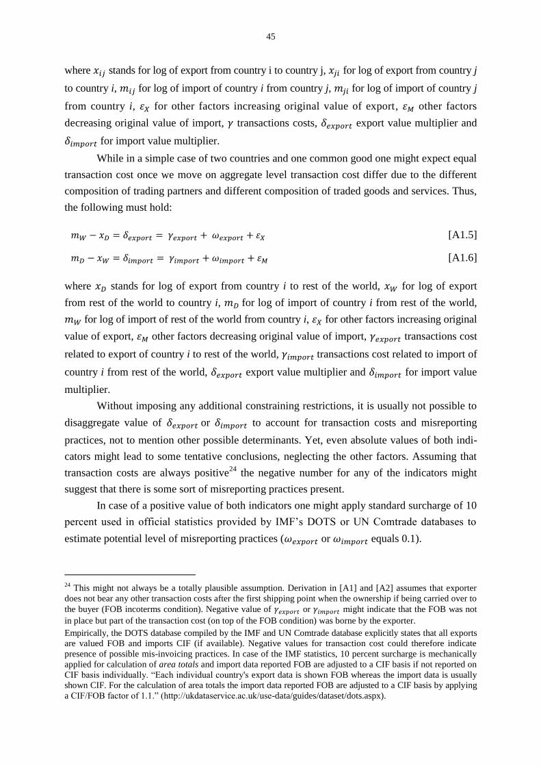
45

where 𝑥𝑖𝑗 stands for log of export from country i to country j, 𝑥𝑗𝑖 for log of export from country j

to country i, 𝑚𝑖𝑗 for log of import of country i from country j, 𝑚𝑗𝑖 for log of import of country j

from country i, 휀𝑋 for other factors increasing original value of export, 휀𝑀 other factors

decreasing original value of import, 𝛾 transactions costs, 𝛿𝑒𝑥𝑝𝑜𝑟𝑡 export value multiplier and

𝛿𝑖𝑚𝑝𝑜𝑟𝑡 for import value multiplier.

While in a simple case of two countries and one common good one might expect equal

transaction cost once we move on aggregate level transaction cost differ due to the different

composition of trading partners and different composition of traded goods and services. Thus,

the following must hold:

𝑚𝑊 − 𝑥𝐷 = 𝛿𝑒𝑥𝑝𝑜𝑟𝑡 = 𝛾𝑒𝑥𝑝𝑜𝑟𝑡 + 𝜔𝑒𝑥𝑝𝑜𝑟𝑡 + 휀𝑋 [A1.5]

𝑚𝐷 − 𝑥𝑊 = 𝛿𝑖𝑚𝑝𝑜𝑟𝑡 = 𝛾𝑖𝑚𝑝𝑜𝑟𝑡 + 𝜔𝑖𝑚𝑝𝑜𝑟𝑡 + 휀𝑀 [A1.6]

where 𝑥𝐷 stands for log of export from country i to rest of the world, 𝑥𝑊 for log of export

from rest of the world to country i, 𝑚𝐷 for log of import of country i from rest of the world,

𝑚𝑊 for log of import of rest of the world from country i, 휀𝑋 for other factors increasing original

value of export, 휀𝑀 other factors decreasing original value of import, 𝛾𝑒𝑥𝑝𝑜𝑟𝑡 transactions cost

related to export of country i to rest of the world, 𝛾𝑖𝑚𝑝𝑜𝑟𝑡 transactions cost related to import of

country i from rest of the world, 𝛿𝑒𝑥𝑝𝑜𝑟𝑡 export value multiplier and 𝛿𝑖𝑚𝑝𝑜𝑟𝑡 for import value

multiplier.

Without imposing any additional constraining restrictions, it is usually not possible to

disaggregate value of 𝛿𝑒𝑥𝑝𝑜𝑟𝑡 or 𝛿𝑖𝑚𝑝𝑜𝑟𝑡 to account for transaction costs and misreporting

practices, not to mention other possible determinants. Yet, even absolute values of both indi-

cators might lead to some tentative conclusions, neglecting the other factors. Assuming that

transaction costs are always positive24

the negative number for any of the indicators might

suggest that there is some sort of misreporting practices present.

In case of a positive value of both indicators one might apply standard surcharge of 10

percent used in official statistics provided by IMF’s DOTS or UN Comtrade databases to

estimate potential level of misreporting practices (𝜔𝑒𝑥𝑝𝑜𝑟𝑡 or 𝜔𝑖𝑚𝑝𝑜𝑟𝑡 equals 0.1).

24

This might not always be a totally plausible assumption. Derivation in [A1] and [A2] assumes that exporter

does not bear any other transaction costs after the first shipping point when the ownership if being carried over to

the buyer (FOB incoterms condition). Negative value of 𝛾𝑒𝑥𝑝𝑜𝑟𝑡 or 𝛾𝑖𝑚𝑝𝑜𝑟𝑡 might indicate that the FOB was not

in place but part of the transaction cost (on top of the FOB condition) was borne by the exporter.

Empirically, the DOTS database compiled by the IMF and UN Comtrade database explicitly states that all exports

are valued FOB and imports CIF (if available). Negative values for transaction cost could therefore indicate

presence of possible mis-invoicing practices. In case of the IMF statistics, 10 percent surcharge is mechanically

applied for calculation of area totals and import data reported FOB are adjusted to a CIF basis if not reported on

CIF basis individually. “Each individual country's export data is shown FOB whereas the import data is usually

shown CIF. For the calculation of area totals the import data reported FOB are adjusted to a CIF basis by applying

a CIF/FOB factor of 1.1.” (http://ukdataservice.ac.uk/use-data/guides/dataset/dots.aspx).

46

The literature on the CIF/FOB factor is relatively large in both depth and scope. In the

first strand of the literature, the CIF/FOB factor measured as simple difference between FOB

volume of export and CIF volume of import is taken as a proxy variable for transaction costs

in international trade. The measurement of transactions costs has a wide range of usage in

different models of international trade (gravity models etc.). The second strand of literature

takes everything that is reported over the 10 percent level of transaction costs as a measurement

of misreporting practices (e.g. Kar and Freitas, 2013) Thirdly, the consistency of trade statistics

among countries is tested by the mirror analysis (statistics) on aggregate or disaggregate level

(e.g. Guo, 2009).

The impact of other factors captured by the coefficients 휀𝑋 and 휀𝑀 might vary from

country to country. In empirical literature the increasing role of re-export is often stressed

when explaining the differences in recorded trade data from bilateral trade partners (Guo,

2009; Cobhan, Jansky and Prats, 2014).25

Other factors falling into this category include

existence of cros-country differences in threshold for recording international transactions,

exchange rate fluctuations or presence of not harmonized trade customs procedures adopted

by countries.26

In the Graph A1 we plot trend lines for both 𝛿𝑒𝑥𝑝𝑜𝑟𝑡 and 𝛿𝑖𝑚𝑝𝑜𝑟𝑡 factors and show the

difference between trend line and actual value for trade with goods for 1997-2014 period.

25

Re-exports (trans-shipments, triangular trade with merchandising) take place when goods enter a custom territo-

ry and leave it to be shipped to other country without being transformed. Countries that usually report high share

of re-export belong to group of countries with either specific geographical location (Netherlands and Belgium in

Europe, Singapore for East Asia, Dubai for Middle East) or special trade status (Hong Kong for China Mainland).

Re-export can significantly worsens trade discrepancies among trade partners due to problems with identification

of country of origin (from importer’s point of view) and country of last known destination (from exporter’s point

of view) principle applied in international trade accounting/reporting. As the re-exporting country serves as

a middle man between country of origin and country of last known destination the likelihood of losing some

significant piece of information on trading partners is increasing with a length of distribution channel.

In one possible scenario country of origin properly identifies country of last known destination as its final

importer and vice versa and re-exporting middle man country will not enter any trade statistics. In other case,

primary exporter identifies re-exporting country as the country of last known destination and final importer identifies

re-exporting country as the country of origin. In both cases, the mirror statistics of international trade remains

unaffected but the geographical distribution of foreign trade across countries is distorted in the second case

(re-exporting country reports increase in both export and import side). However, other possible combinations are

likely to occur that would have a direct impact on quality of international trade statistics: a) country of origin

identifies re-exporting country as the last known destination country (importer) but the true last known destination

will be able to identify country of origin as the primary exporter; b) country of origin does not identify re-exporting

country and only the true last known destination country is recorded as the final importer but the true last known

destination country identifies re-exporting country as the country of origin. In both cases, different identification

of initial exporter and final importer are a source of discrepancies in mirror trade statistics, thus affect our

CIF/FOB ratio through epsilon coefficients. 26

Different thresholds for small transactions category between trading partners that do not enter trade statistics

distort mirror trade statistics, thus affect our CIF/FOB ratio through epsilon coefficient.

Secondly, trade volumes are usually collected and reported in local currency and then converted by average US

dollar exchange rate valid for the specific period. Discrepancies between trade volumes measured in this way

might occur if the exchange rate between trade partners shows a higher volatility, assuming the trade volume

throughout the period is not constant. Then the average US dollar exchange rate used for conversion will introduce

discrepancies in mirror trade statistics.

47

G r a p h A1

Evolution of export and import factors in Slovakia (1997-2014)

Note: Export and import factors are calculated as in [A1.5] and [A1.6]. Series are seasonally adjusted. Trend is

extracted using Hodrick-Prescott filter with lambda 1600. Export series adjusted for transactions costs is calculated

as the difference between export factor variable and trend line of the import factor variable.

Import factor stays over the 10 percent threshold for most of the time before EU ac-

cession in 2004. Minimization of transaction costs due to the EU accession and euro adoption

in 2009 has been translated into steady decrease in long-term trend with import factor values

effectively achieving minimum levels in 2010 and fluctuating around zero since then. There

are three notable peaks recognizable in the overall relatively smooth behavior of the import

factor: last quarter of 1998, third quarter of 2001 and first quarter of 2009. Behavior in 2009

partially supports the hypothesis of one-time hit due to the euro changeover in the import

prices as the effect of this hit on import factor dies out very quickly. Taking the value of long-

term trend as a benchmark for average transaction costs, the level of import overvaluation

ranges from 2 (3q2009) to 12 percent (1q2009) during the year 2009 and then basically stabi-

lizes around zero.

The behavior of the export factor introduces some pressing issues. Assuming that the

long-term trend of the import factor reasonably captures economically justified transaction

costs, level of overestimation of export remains anchored at approximately 15 percent for

the pre-2010 period. Thus, almost entire history of foreign trade with goods is marked with

significant over-recording issues except short periods of “normal” times during years 2003-2004

and post-2010 years. Mechanically, these significant mis-invoicing practices might stem from

48

three sources: (1) foreign trade partners might willingly engage in underreporting practices of

their import, (2) Slovak businesses might enjoy being involved in over-reporting of their foreign

export values, or (3) different reporting standards consistently overestimate value of Slovak

export. While all three cases might be true to some extent, we are prone to attach higher

explanatory power to the third source of disturbances. As discussed in the recent report by

NBS (2015), shift in reporting practices from cross-border to national concept has led to

a significant decline in net export balance, especially for years 2009-2011. As apparent from

the Graph A1, an important break in the adjusted export factor series that occurred in 2010 has

effectively moved mean of the series to zero. In other words, change in foreign trade statistics

reporting system might have corrected discrepancy in the export mis-recording factor that has

remained in negative numbers since 2005. On top of that, negative trend in series that started in

2005 might be, at least partially, attributed to the EU accession that had let to breakdown of

linkages between cross-border movement of goods and change of ownership.

49

APPENDIX 2

Link between Net errors and omissions and open macroeconomic identity

The theory presented here represents a conjunction of approaches described in Fausten

and Pickett (2004), Tang and Fausten (2012) and Tang (2013).

In theory, link between NeO and other macroeconomic variables is built upon the

open-macroeconomic identity for savings-investment gap and balance of payments double-

accounting principle. Suppose that variables with hat on top represent officially recorded values

while variables without any markings stand for their true unobserved realizations. Then the

reported net errors and omissions can be expressed as the following:

𝐶𝐴 = 𝐶�̂� + 𝐸𝑂𝐶𝐴 [A2.1]

𝐶𝐹𝐴 = 𝐶𝐹�̂� + 𝐸𝑂𝐶𝐹𝐴 [A2.2]

𝐸𝑂 = −𝐶�̂�(. ) − 𝐶𝐹�̂�(. ) [A2.3]

𝐸𝑂 = −𝐶�̂�(𝑦(−), 𝑦∗(+), 𝑟𝑒𝑟(+)) − 𝐶𝐹�̂�(𝑟(+), 𝑟∗(−)) [A2.4]

where 𝑦 stands for real domestic output, 𝑦∗ real foreign output, 𝑟𝑒𝑟 real exchange rate, 𝑟

domestic real interest rate, 𝑟∗ foreign real interest rate, 𝐶𝐴 current account balance, 𝐶𝐹𝐴 capital

and financial account balance and 𝐸𝑂 net errors and omissions. It is assumed that increase in

real exchange rate brings about increase in price competitiveness of domestically-produced

goods and services.

Taking into account savings-investment relationship in a small open economy, the net

errors and omissions are given by the following expression:

𝑆𝑔 − 𝐼 = 𝐶�̂� + 𝐸𝑂𝐶𝐴 [A2.5]

−(𝑆𝑔 − 𝐼) = 𝐶𝐹�̂� + 𝐸𝑂𝐶𝐹𝐴 [A2.6]

−(𝑆𝑔 − 𝐼) − 𝐶𝐹�̂� + 𝐸𝑂𝐶𝐴 = 𝐸𝑂𝐶𝐹𝐴 + 𝐸𝑂𝐶𝐴 = 𝐸𝑂 [A2.7]

𝐸𝑂 = −𝑆𝑔(𝑦(+), 𝑟(+)) + 𝐼(𝑟(−)) − 𝐶𝐹�̂�(𝑟(+), 𝑟∗(−)) + 𝐸𝑂𝐶𝐴 [A2.8]

𝐸𝑂 = 𝑓(𝑦(−), 𝑟(−), 𝑟∗(+)) + 𝐸𝑂𝐶𝐴 [A2.9]

where 𝑆𝑔 stands for gross savings, 𝐼 domestic investments, 𝑦 real domestic output, 𝑦∗ real

foreign output, 𝑟𝑒𝑟 real exchange rate, 𝑟 domestic real interest rate, 𝑟∗ foreign real interest

rate, 𝐶𝐴 current account balance, 𝐶𝐹𝐴 capital and financial account balance and 𝐸𝑂 net errors

and omissions.

Macroeconomic identity states that the Net errors and omissions part from the balance

of payments should be indirectly driven by fundamental factors influencing export and import

decisions of domestic and foreign economic agents (domestic and foreign income, real exchange

rate) and their investments portfolio allocation (interest rate spread).