Adam Szustalewicz Modelowanie zjawisk przyrodniczych W.14 2014.01.22

Wykªad 14: Zagadnienia sztywne � ci¡g dalszy

1 Uzupeªnienie zagadnie«, interpolacja wyników numerycznych

B¦dziemy rozwi¡zywa¢ kilkoma metodami: ode15s.m , ode113.m , ode45.m RR postaci

function dy = deriv(t,y)

dy = lambda*y + (1-lambda)*cos(t) - (1+lambda)*sin(t);

num_fcn_eval = num_fcn_eval + 1;

end % deriv

o rozwi¡zaniu dokªadnym function true = true_soln(t)

true = sin(t) + cos(t);

end % true_soln

dla kilku warto±ci parametru λ: -10 , -1000 , -10000 .

Obejrzyjmy informacje o funkcjach:

ode45 Solve non-sti� di�erential equations, medium order method.[TOUT,YOUT] = ode45(ODEFUN,TSPAN,Y0) with TSPAN = [T0 TFINAL]integrates the system of di�erential equations y' = f(t,y) from time T0 to TFINAL with initial conditions Y0.ODEFUN is a function handle.For a scalar T and a vector Y, ODEFUN(T,Y) must return a column vector corresponding to f(t,y).Each row in the solution array YOUT corresponds to a time returned in the column vector TOUT.To obtain solutions at speci�c times T0,T1,...,TFINAL (all increasing or all decreasing), useTSPAN = [T0 T1 ... TFINAL].[TOUT,YOUT]= ode45(ODEFUN,TSPAN,Y0,OPTIONS) solves as above with default integration properties replacedby values in OPTIONS, an argument created with the ODESET function. See ODESET for details.SOL = ode45(ODEFUN,[T0 TFINAL],Y0...) returns a structure that can be used with DEVAL to evaluate thesolution or its �rst derivative at any point between T0 and TFINAL.

ode113 Solve non-sti� di�erential equations, variable order method.

ode15s Solve sti� di�erential equations and DAEs, variable order method.ode15s can solve problems M(t,y)*y' = f(t,y) with mass matrix M(t,y).The Jacobian matrix df/dy is critical to reliability and e�ciency. Use ODESET to set 'Jacobian' to a function handleFJAC if FJAC(T,Y) returns the Jacobian df/dy or to the matrix df/dy if the Jacobian is constant. If the 'Jacobian'option is not set (the default), df/dy is approximated by �nite di�erences.

1.1 Interpolacja wyników numerycznych

� help devalDEVAL Evaluate the solution of a di�erential equation problem.SXINT = DEVAL(SOL,XINT) evaluates the solution of a di�erential equation problem at all the entries of the vectorXINT. SOL is a structure returned by an initial value problem solver (ODE45, ODE23, ODE113, ODE15S, ODE23S,ODE23T, ODE23TB, ODE15I), the boundary value problem solver (BVP4C), or the solver for delay di�erentialequations (DDE23).The elements of XINT must be in the interval [SOL.x(1) SOL.x(end)].For each I, SXINT(:,I) is the solution corresponding to XINT(I).

1.2 Pocz¡tek programu testowego

function test_ode15s(lambda, relerr, abserr)

options = odeset('RelTol', relerr, 'AbsTol', abserr);

t_begin = 0; t_end = 20;

y_initial = true_soln(t_begin);

num_fcn_eval = 0;

soln = ode15s(@deriv, [t_begin,t_end], y_initial, options);

h_plot = (t_end-t_begin)/1000; t_plot = t_begin:h_plot:t_end;

y_plot = deval(soln,t_plot);

figure, plot(soln.x,soln.y,'o',t_plot,y_plot)

y_true_nodes = true_soln(soln.x); error_nodes = y_true_nodes - soln.y;

y_true = true_soln(t_plot); error = y_true - y_plot;

figure, plot(soln.x,error_nodes,'o',t_plot,error)

1

Adam Szustalewicz Modelowanie zjawisk przyrodniczych W.14 2014.01.22

� help odesetodeset Create/alter ODE OPTIONS structure.OPTIONS = odeset('NAME1',VALUE1,'NAME2',VALUE2,...) creates an integrator options structure OPTIONS inwhich the named properties have the speci�ed values.odeset with no input arguments displays all property names and their possible values.

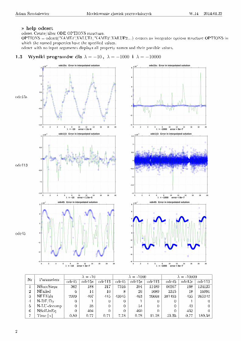
1.3 Wyniki programów dla λ = −10 , λ = −1000 i λ = −10000

ode15s

0 2 4 6 8 10 12 14 16 18 20−1.5

−1

−0.5

0

0.5

1

1.5

2x 10

−6 ode15s: Error in interpolated solution

λ = −10 error < 2e−6

ode113

0 2 4 6 8 10 12 14 16 18 20−1.5

−1

−0.5

0

0.5

1x 10

−5 ode113: Error in interpolated solution

λ = −10 error < 1.5e−5

ode45

0 2 4 6 8 10 12 14 16 18 20−3

−2

−1

0

1

2

3x 10

−7 ode45: Error in interpolated solution

λ = −10 error < 3e−7

0 2 4 6 8 10 12 14 16 18 20−4

−2

0

2

4

6

8x 10

−7 ode15s: Error in interpolated solution

λ = −1000 error < 8e−7

0 2 4 6 8 10 12 14 16 18 20−2

−1.5

−1

−0.5

0

0.5

1

1.5x 10

−5 ode113: Error in interpolated solution

λ = −1000 error < 8e−7

0 2 4 6 8 10 12 14 16 18 20−8

−6

−4

−2

0

2

4

6

8x 10

−7 ode45: Error in interpolated solution

λ = −1000 error < 8e−7

λ = -10 λ = -1000 λ = -10000Nr Parameters ode45 ode15s ode113 ode45 ode15s ode113 ode45 ode15s ode1131 NSuccSteps 362 188 217 7316 204 12489 60267 198 1241252 NFailed 6 14 10 8 26 1689 3315 18 169913 NFEVals 2209 407 445 43945 463 26668 381493 435 2652424 N-DF/Dy 0 1 0 0 1 0 0 1 05 N-LU-decomp 0 38 0 0 54 0 0 43 06 NSolLinEq 0 404 0 0 460 0 0 432 07 Time [ s ] 0.80 0.77 0.71 7.78 0.78 11.58 53.35 0.77 189.38

2

Adam Szustalewicz Modelowanie zjawisk przyrodniczych W.14 2014.01.22

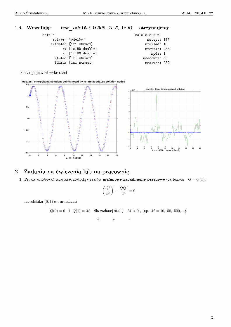
1.4 Wywoªuj¡c test_ode15s(-10000, 1e-6, 1e-6) otrzymujemy

soln =

solver: 'ode15s'

extdata: [1x1 struct]

x: [1x189 double]

y: [1x189 double]

stats: [1x1 struct]

idata: [1x1 struct]

soln.stats =

nsteps: 198

nfailed: 18

nfevals: 435

npds: 1

ndecomps: 43

nsolves: 432

z nast¦puj¡cymi wykresami

0 2 4 6 8 10 12 14 16 18 20−1.5

−1

−0.5

0

0.5

1

1.5ode15s: Interpolated solution: points noted by ’o’ are at ode15s solution nodes

λ = −10000

0 2 4 6 8 10 12 14 16 18 20−2

−1

0

1

2

3

4

5

6x 10

−7 ode15s: Error in interpolated solution

λ = −10000 error < 6e−7

2 Zadania na ¢wiczenia lub na pracowni¦

1. Prosz¦ spróbowa¢ rozwi¡za¢ metod¡ strzaªów nieliniowe zagadnienie brzegowe dla funkcji Q = Q(x) :(Q ′

x2

)′

− QQ ′

x4= 0

na odcinku (0, 1) z warunkami:

Q(0) = 0 i Q(1) = M dla zadanej staªej M > 0 , (np. M = 10, 50, 500, ...).

* * *

3