Modeling and Optimization in Science and Technologies

Xin-She YangGebrail BekdaşSinan Melih Nigdeli Editors

Metaheuristics and Optimization in Civil Engineering

Modeling and Optimization in Scienceand Technologies

Volume 7

Series editors

Srikanta Patnaik, SOA University, Orissa, Indiae-mail: patnaik_srikanta@yahoo.co.in

Ishwar K. Sethi, Oakland University, Rochester, USAe-mail: isethi@oakland.edu

Xiaolong Li, Indiana State University, Terre Haute, USAe-mail: Xiaolong.Li@indstate.edu

Editorial Board

Li Cheng, The Hong Kong Polytechnic University, Hong KongJeng-Haur Horng, National Formosa University, Yulin, TaiwanPedro U. Lima, Institute for Systems and Robotics, Lisbon, PortugalMun-Kew Leong, Institute of Systems Science, National University of SingaporeMuhammad Nur, Diponegoro University, Semarang, IndonesiaLuca Oneto, University of Genoa, ItalyKay Chen Tan, National University of Singapore, SingaporeSarma Yadavalli, University of Pretoria, South AfricaYeon-Mo Yang, Kumoh National Institute of Technology, Gumi, South KoreaLiangchi Zhang, The University of New South Wales, AustraliaBaojiang Zhong, Soochow University, Suzhou, ChinaAhmed Zobaa, Brunel University, Uxbridge, Middlesex, UK

About this Series

The book series Modeling and Optimization in Science and Technologies (MOST)publishes basic principles as well as novel theories and methods in the fast-evolvingfield of modeling and optimization. Topics of interest include, but are not limited to:methods for analysis, design and control of complex systems, networks andmachines; methods for analysis, visualization and management of large data sets;use of supercomputers for modeling complex systems; digital signal processing;molecular modeling; and tools and software solutions for different scientific andtechnological purposes. Special emphasis is given to publications discussing noveltheories and practical solutions that, by overcoming the limitations of traditionalmethods, may successfully address modern scientific challenges, thus promotingscientific and technological progress. The series publishes monographs, contributedvolumes and conference proceedings, as well as advanced textbooks. The maintargets of the series are graduate students, researchers and professionals working atthe forefront of their fields.

More information about this series at http://www.springer.com/series/10577

Xin-She Yang • Gebrail BekdaşSinan Melih NigdeliEditors

Metaheuristicsand Optimization in CivilEngineering

123

EditorsXin-She YangSchool of Science and TechnologyMiddlesex UniversityLondonUK

Gebrail BekdaşFaculty of EngineeringIstanbul UniversityIstanbulTurkey

Sinan Melih NigdeliFaculty of EngineeringIstanbul UniversityIstanbulTurkey

ISSN 2196-7326 ISSN 2196-7334 (electronic)Modeling and Optimization in Science and TechnologiesISBN 978-3-319-26243-7 ISBN 978-3-319-26245-1 (eBook)DOI 10.1007/978-3-319-26245-1

Library of Congress Control Number: 2015954625

Springer Cham Heidelberg New York Dordrecht London© Springer International Publishing Switzerland 2016This work is subject to copyright. All rights are reserved by the Publisher, whether the whole or partof the material is concerned, specifically the rights of translation, reprinting, reuse of illustrations,recitation, broadcasting, reproduction on microfilms or in any other physical way, and transmissionor information storage and retrieval, electronic adaptation, computer software, or by similar or dissimilarmethodology now known or hereafter developed.The use of general descriptive names, registered names, trademarks, service marks, etc. in thispublication does not imply, even in the absence of a specific statement, that such names are exempt fromthe relevant protective laws and regulations and therefore free for general use.The publisher, the authors and the editors are safe to assume that the advice and information in thisbook are believed to be true and accurate at the date of publication. Neither the publisher nor theauthors or the editors give a warranty, express or implied, with respect to the material contained herein orfor any errors or omissions that may have been made.

Printed on acid-free paper

Springer International Publishing AG Switzerland is part of Springer Science+Business Media(www.springer.com)

Preface

Almost all design problems in engineering can be considered as optimizationproblems and thus require optimization techniques to solve. However, as mostreal-world problems are highly nonlinear, traditional optimization methods usuallydo not work well. The current trend is to use evolutionary algorithms and meta-heuristic optimization methods to tackle such nonlinear optimization problems.Metaheuristic algorithms have gained huge popularity in recent years. Thesemetaheuristic algorithms include genetic algorithms, particle swarm optimization,bat algorithm, cuckoo search, differential evolution, firefly algorithm, harmonysearch, flower pollination algorithm, ant colony optimization, bee algorithms, andmany others. The popularity of nature-inspired metaheuristic algorithms can beattributed to their good characteristics because these algorithms are simple, flexible,efficient, and adaptable, and yet easy to implement. Such advantages make themversatile to deal with a wide range of optimization problems without much a prioriknowledge about the problem to be solved.

Metaheuristic algorithms play an important role in the optimum design ofcomplex engineering problems when analytical approaches and traditional methodsare not effective for solving nonlinear design problems in civil engineering.Generally speaking, these design problems are highly nonlinear with complexconstraints, and thus are also highly multimodal. These design constraints oftencome from design requirements and security measures such as the stresses on themembers due to external loading, environmental factors, and usability under serviceloads. A mathematical solution may be the best approach in an ideal world, but inengineering designs, the values of a design variable such as mass or length must berealistic; for example, quantities must be nonnegative. In addition, such designvalues must correspond to something that can be manufacturable in practice.

For all engineering disciplines, optimization is crucially important in the designprocess so as to find a good balance between economy and security that are theprimary goals of designs. Aesthetics and practicability are also important inreal-world applications. Civil engineering is probably the oldest engineering dis-cipline and it has always been linked to the construction and realization of

v

civilization. In fact, optimization may be more relevant in civil engineering than inother engineering disciplines. For example, in designing a non-critical machine partin mechanical engineering, the stresses on the part must not exceed certain limits. Ifa stronger part is used, it may become too expensive. On the other hand, a weakerpart may still be able to make the machine work properly, but in time such weakparts can be worn off or damaged. However, such parts may be easy to be replacedat low costs. If this is the case, machine serviceability can be maintained in practice.But in civil engineering, structural integrity and safety may impose stringentrestrictions on the structural members that may not be easily replaced. In such cases,all design constraints and the best possible balance between security and economymust be found without risking lives. In addition, sometimes, the minor improve-ment may not be as important as robustness in applications. A robust design shouldbe able to handle uncertainties in terms of material properties, manufacturing tol-erance, and load irregularity in service. Due to complexity and a large number ofdesign constraints in civil engineering, traditional methods often struggle to copewith such high nonlinearity and multimodality. Thus, metaheuristic optimizationmethods have become important tools in the optimum design in civil engineering.

This edited book strives to summarize the latest developments in optimizationand metaheuristic algorithms with emphasis on applications in civil engineering.Topics include the overview of meteaheuristic algorithms and optimization,structural optimization by flower pollination algorithm, steel design by swarmintelligence, optimum seismic design of steel frames by bat algorithm, 3D trussoptimization by genetic algorithms, reactive power optimization by cuckoo search,structural design by harmony search, asphalt pavement management, reinforcedconcrete beam design, transport infrastructure planning, water distribution net-works, capacitated vehicle routing, slope stability problems, and others. Therefore,this timely book can serve as an ideal reference for graduates, lecturers, engineers,and researchers in civil engineering, mechanical engineering, transport andgeotechnical engineering. It can also serve as a timely reference for relevant uni-versity courses in all disciplines in civil engineering.

We would like to thank the editors and staff at Springer for their help andprofessionalism. Last but not least, we thank our families for their help and support.

June 2015 Xin-She YangGebrail Bekdaş

Sinan Melih Nigdeli

vi Preface

Contents

Review and Applications of Metaheuristic Algorithms in CivilEngineering . . . . . . . . . . . . . . . . . . . . . . . . . . . . . . . . . . . . . . . . . . . . 1Xin-She Yang, Gebrail Bekdaş and Sinan Melih Nigdeli

Application of the Flower Pollination Algorithm in StructuralEngineering . . . . . . . . . . . . . . . . . . . . . . . . . . . . . . . . . . . . . . . . . . . . 25Sinan Melih Nigdeli, Gebrail Bekdaş and Xin-She Yang

Use of Swarm Intelligence in Structural Steel Design Optimization . . . . 43Mehmet Polat Saka, Serdar Carbas, Ibrahim Aydogdu and Alper Akin

Metaheuristic Optimization in Structural Engineering . . . . . . . . . . . . . 75S.O. Degertekin and Zong Woo Geem

Performance-Based Optimum Seismic Design of Steel DualBraced Frames by Bat Algorithm . . . . . . . . . . . . . . . . . . . . . . . . . . . . 95Saeed Gholizadeh and Hamed Poorhoseini

Genetic Algorithms for Optimization of 3D Truss Structures . . . . . . . . 115Vedat Toğan and Ayşe Turhan Daloğlu

Hybrid Meta-heuristic Application in the Asphalt PavementManagement System . . . . . . . . . . . . . . . . . . . . . . . . . . . . . . . . . . . . . . 135Fereidoon Moghadas Nejad, Ashkan Allahyari Nik and H. Zakeri

Optimum Reinforced Concrete Design by HarmonySearch Algorithm . . . . . . . . . . . . . . . . . . . . . . . . . . . . . . . . . . . . . . . . 165Gebrail Bekdaş, Sinan Melih Nigdeli and Xin-She Yang

Reactive Power Optimization in Wind Power PlantsUsing Cuckoo Search Algorithm . . . . . . . . . . . . . . . . . . . . . . . . . . . . . 181K.S. Pandya, J.K. Pandya, S.K. Joshi and H.K. Mewada

vii

A DSS-Based Honeybee Mating Optimization (HBMO)Algorithm for Single- and Multi-objective Design of WaterDistribution Networks . . . . . . . . . . . . . . . . . . . . . . . . . . . . . . . . . . . . . 199Omid Bozorg Haddad, Navid Ghajarnia, Mohammad Solgi,Hugo A. Loáiciga and Miguel Mariño

Application of the Simulated Annealing Algorithmfor Transport Infrastructure Planning . . . . . . . . . . . . . . . . . . . . . . . . . 235Ana Laura Costa, Maria Conceição Cunha, Paulo A.L.F. Coelhoand Herbert H. Einstein

A Hybrid Bat Algorithm with Path Relinking for the CapacitatedVehicle Routing Problem . . . . . . . . . . . . . . . . . . . . . . . . . . . . . . . . . . . 255Yongquan Zhou, Qifang Luo, Jian Xie and Hongqing Zheng

Hybrid Metaheuristic Algorithms in Geotechnical Engineering . . . . . . . 277Y.M. Cheng

viii Contents

Contributors

Alper Akin Thomas & Betts Corporation, Meyer Steel Structures, Memphis, TN,USA

Ashkan Allahyari Nik Department of Civil Engineering, Science and ResearchBranch, Islamic Azad University, Tehran, Iran

Ibrahim Aydogdu Department of Civil Engineering, Akdeniz University,Antalya, Turkey

Gebrail Bekdaş Department of Civil Engineering, Istanbul University, Avcılar,Istanbul, Turkey

Omid Bozorg Haddad University of Tehran, Tehran, Iran

Serdar Carbas Department of Civil Engineering, Karamanoglu MehmetbeyUniversity, Karaman, Turkey

Y.M. Cheng Department of Civil and Environmental Engineering, Hong KongPolytechnic University, Hung Hom, Hong Kong

Paulo A.L.F. Coelho Department of Civil Engineering, University of Coimbra,Coimbra, Portugal

Ana Laura Costa Department of Civil Engineering, University of Coimbra,Coimbra, Portugal

Maria Conceição Cunha Department of Civil Engineering, University ofCoimbra, Coimbra, Portugal

Ayşe Turhan Daloğlu Department of Civil Engineering, Karadeniz TechnicalUniversity, Trabzon, Turkey

S.O. Degertekin Department of Civil Engineering, Dicle University, Diyarbakir,Turkey

ix

Herbert H. Einstein Department of Civil and Environmental Engineering,Massachusetts Institute of Technology, Cambridge, USA

Zong Woo Geem Department of Energy IT, Gachon University, Seongnam, SouthKorea

Navid Ghajarnia University of Tehran, Tehran, Iran

Saeed Gholizadeh Department of Civil Engineering, Urmia University, Urmia,Iran

S.K. Joshi Department of Electrical Engineering, The M.S. University of Baroda,Vadodara, India

Hugo A. Loáiciga University of California, Santa Barbara, Santa Barbara, CA,USA

Qifang Luo College of Information Science and Engineering, Guangxi Universityfor Nationalities, Nanning, China

Miguel Mariño University of California, Davis, Davis, CA, USA

H.K. Mewada Department of Electronics and Communications, CSPIT, CharotarUniversity of Science and Technoloogy, Changa, India

Fereidoon Moghadas Nejad Department of Civil and Environment Engineering,Amirkabir University of Technology, Tehran, Iran

Sinan Melih Nigdeli Department of Civil Engineering, Istanbul University,Avcılar, Istanbul, Turkey

J.K. Pandya Department of Civil Engineering, Dharmsinh Desai University,Nadiad, India

K.S. Pandya Department of Electrical Engineering, CSPIT, Charotar Universityof Science and Technology, Changa, India

Hamed Poorhoseini Department of Civil Engineering, Urmia University, Urmia,Iran

Mehmet Polat Saka Department of Civil Engineering, University of Bahrain, IsaTown, Bahrain

Mohammad Solgi University of Tehran, Tehran, Iran

Vedat Toğan Department of Civil Engineering, Karadeniz Technical University,Trabzon, Turkey

Jian Xie College of Information Science and Engineering, Guangxi University forNationalities, Nanning, China

Xin-She Yang Design Engineering and Mathematics, School of Science andTechnology, Middlesex University, The Burroughs, London, UK

x Contributors

H. Zakeri Amirkabir Artificial Intelligence and Image Processing Lab (Attain),Department of Civil and Environment Engineering, Amirkabir University ofTechnology, Tehran, Iran

Hongqing Zheng College of Information Science and Engineering, GuangxiUniversity for Nationalities, Nanning, China

Yongquan Zhou College of Information Science and Engineering, GuangxiUniversity for Nationalities, Nanning, China; Guangxi High School KeyLaboratory of Complex System and Computational Intelligence, Nanning, China

Contributors xi

Review and Applications of MetaheuristicAlgorithms in Civil Engineering

Xin-She Yang, Gebrail Bekdaş and Sinan Melih Nigdeli

Abstract Many design optimization problems in civil engineering are highlynonlinear and can be challenging to solve using traditional methods. In many cases,metaheurisitc algorithms can be an effective alternative and thus suitable in civilengineering applications. In this chapter, metaheuristic algorithms in civil engi-neering problems are briefly presented and recent applications are discussed. Twocase studies such as the optimization of tuned mass dampers and cost optimizationof reinforced concrete beams are analyzed.

Keywords Metaheuristic algorithms � Civil engineering � Optimization

1 Introduction

Metaheuristic algorithms play a great role in the optimum design of complexengineering problems when analytical approaches and traditional methods are noteffective for solving nonlinear design problems in civil engineering. Generallyspeaking, these design problems are highly nonlinear with complex constraints, andthus are also highly multimodal. These design constraints often come from design

X.-S. Yang (&)Design Engineering and Mathematics, Middlesex University, The Burroughs,London NW4 4BT, UKe-mail: x.yang@mdx.ac.uk; xy227@cam.ac.uk

X.-S. YangSchool of Science and Technology, Middlesex University, The Burroughs,London NW4 4BT, UK

G. Bekdaş � S.M. NigdeliDepartment of Civil Engineering, Istanbul University, 34320 Avcılar, Istanbul, Turkeye-mail: bekdas@istanbul.edu.tr

S.M. Nigdelie-mail: melihnig@istanbul.edu.tr

© Springer International Publishing Switzerland 2016X.-S. Yang et al. (eds.), Metaheuristics and Optimization in Civil Engineering,Modeling and Optimization in Science and Technologies 7,DOI 10.1007/978-3-319-26245-1_1

1

requirements and security measures such as stresses on the members due to externalloading, environmental factors, and usability under service loads. In addition to thedesign constraints, solution ranges for the design variables must be defined.A mathematical solution may be the best approach in an ideal world, but inengineering design, if a variable is a mass or a length, the value of the designvariable must be realistic, for example, it cannot be negative. In addition, the designvalues must correspond to something that can be manufacturable in practice.

For all engineering disciplines, optimization is needed in the design in order tofind a good balance between economy and security which are the primary goals ofdesigns and engineers should not ignore any of these two goals. Esthetics andpracticability are the other important goals which are also important in manyspecific design problems. Thus, these goals should also be considered in addition tothe primary goals, if needed.

Civil engineering is the oldest engineering discipline and it has been linked toone of humanity’s most important needs—the construction and realization of civ-ilization. In fact, optimization may be more relevant in civil engineering than inother engineering disciplines. For example, in designing a machine part inmechanical engineering, the stresses on the part must not exceed the securitymeasures. If we produce a stronger part, it will be too expensive. If the part is notstrong enough, it can serve, but in time, the part can be damaged. In that case, thispart may be replaced with a new one and serviceability of the machine can still besustained. This process is normal for mechanical engineering designs, but wecannot replace a structural member easily in civil engineering. Also, in civilengineering, big and complex systems are investigated. In that case, we need toconsider all design constraints and the best balance between security and economymust be found without risking lives. Due to various design constraints, mathe-matical optimization may not be effective in civil engineering. Thus, metaheuristicmethods are important in the optimum design of civil engineering.

In this chapter, metaheuristic algorithms used in civil engineering will be pre-sented with some literature reviews. In addition, two optimization case studies inapplications will be presented in detail. These examples include the optimization ofreinforced concrete beams and tuned dampers for the reduction of vibrations.

2 Metaheuristic Algorithms

In engineering, an optimum design problem can be written in mathematical form as

Minimize fi xð Þ; x 2 Rn; ði ¼ 1; 2; . . .NÞ ð1Þ

2 X.-S. Yang et al.

subject to

hj xð Þ; j ¼ 1; 2; . . .; Jð Þ; ð2Þ

gk xð Þ� 0; k ¼ 1; 2; . . .;Kð Þ ð3Þ

where

x ¼ x1; x2; . . .; xnð ÞT ; i ¼ 1; 2; . . .; nð Þ ð4Þ

is the design vector containing design variables. The objective functions (fi (x)),design constraints about equalities (hj (x)), and inequalities (gi (x)) are the functionof the design vector (x). In an optimization process using metaheuristic algorithms,design variables are randomly assigned and then, the objective functions and designconstraints are calculated. Design constraints are generally considered by using apenalized objective function. If a particular set of values of design variables is notsuitable for a design constraint, the objective function, which needs to be mini-mized, should be increased with some penalty.

The set of design variables, or the design vector, is generated several times (orthe number of population) and stored as a matrix containing possible solutions. Thisis the initial part of the algorithm and the process is similar for all metaheuristicalgorithms. After this initial process, the aim is to try to improve the results basedon the special principles of the algorithm of interest. These principles are differentfor each metaheuristic algorithm and are often inspired by or related to a biologicalor natural process. Metaheuristic algorithms inspired from observations of a processusually provide a set of updating equations that can be used to update the existingdesign variables during iteration.

In this section, several metaheuristic algorithms are summarized and the relevantliterature studies concerning these algorithms are also discussed.

2.1 Genetic Algorithm

Genetic algorithm (GA) is one of the oldest metaheuristic algorithms. It is based onCharles Darwin’s theory of natural selection. The properties include the crossoverand recombination, mutation and selection by Holland [1]. The procedure of GAcan be summarized in the following seven steps:Step 1 The optimization objective is encoded.Step 2 A fitness function or criterion for selection of an individual is defined.Step 3 A population of individuals is initialized.Step 4 The fitness function is evaluated for all individuals.Step 5 A new population is generated using the rules of natural selection. These

rules are crossover, mutation, and proportionate reproduction.

Review and Applications of Metaheuristic Algorithms … 3

Step 6 The population is evolved until a defined stopping criterion is met.Step 7 The results are decoded so as to obtain the solutions to the design problem.

The application of GA in civil and structural engineering dates back to 1986,when Goldberg and Samtoni used GA for the optimum design of a 10-bar trusssystem [2]. Until now, GA and its variants have been successfully employed inoptimization of structural engineering problems [3]. Recent applications arestructural system identification [4], design of long-span bridges [5], topologyoptimization of steel space-frame roof structures [6], truss topology optimization[7], and many others. Transportation engineering is also a major application area ofGA. Recently, several approaches to urban traffic flow [8], traffic signal coordi-nation problem [9], emergency logistic scheduling [10], and calibration of railtransit assignment models are proposed [11].

2.2 Simulated Annealing

Annealing is a process in materials science. In the annealing process, a metal isheated so that its structure can rearrange during slow cooling so as to increase theductility and strength of the metal. During such controlled cooling, atoms arrangeinto a low energy state (crystallized state). If the cooling process is quick, apolycrystalline state occurs which is corresponding to a local minimum energy. Inthe simulated annealing (SA) algorithm, Kirkpatrick et al. [12] and Cerny [13] usedthe annealing process as an inspiration.

SA has been used to solve many optimization problems in civil engineering andthe recent applications are as follows. Costa et al. employed SA for planninghigh-speed rail systems [14]. Tong et al. used an improved SA in optimumplacement of sensors [15]. A genetic SA algorithm is employed in the collapseoptimization for domes under seismic excitation [16]. Server systems weredesigned with an SA-based procedure by Karovic and Mays [17]. SA was also usedin thermal building optimization by Junghans and Darde [18].

2.3 Ant Colony Optimization

Ants live in a colony and the population of their colony is between 2 and 25millions. They can lay scent chemicals or pheromone as a means to communicate.Each ant follows pheromone trails, and when exploring the sounding, more pher-omone will be laid from/to the food source. Their behavior can form someemerging characteristics and the ant colony optimization algorithm was developedby Marco Dorigo in 1992 [19].

4 X.-S. Yang et al.

Ant colony optimization (ACO) has also been applied for several structuralengineering problems [3]. Researchers continue to study new applications of civilengineering problems by employing ACO. Recently, multi-compartment vehiclerouting problem [20], traffic engineering problems [21], determination problem ofnoncircular critical slip surface in slope stability analysis [22], and multiobjectivestructural optimization problems [23] were solved by ACO.

2.4 Particle Swarm Optimization

In 1995, Kennedy and Ebarhart [24] developed particle swarm optimization(PSO) which imitates the behavior of social swarms such as ant colonies, bees, andbird flocks. PSO is a population-based metaheuristic algorithm. In a swarm, particlesare randomly generated and new solutions are updated in an iterative manner. Thesolution particles tend to move toward the current best location, while they move tonew locations. Since all particles tend to be the current best solution, the effec-tiveness of population-based algorithm can be easily recognized if the best solutionis an approach to the true global optimality. Compared to GA, PSO uses real-numberstrings and encoding or decoding of the parameters into binary strings is not needed.

Swarm intelligence applications of structural design [25] and several civilengineering applications [26] were recently presented. Most recent applications arethe design of tall buildings [27], size optimization of trusses [28], slope stabilityanalyzing [29], and water distribution systems [30].

2.5 Harmony Search

Harmony search (HS) algorithm is a music-based metaheuristic algorithm. It wasdeveloped by Geem et al. [31] after observation of a musician’s performance.Musicians search the best harmony by playing harmonic music pieces. Similarly,the objective function of an engineering problem can be considered as a harmony.In a musical performance, the musician plays notes and may modify these noteswhen needed. The new notes may be similar to a favorite note or a new song. Themajor application of HS in civil engineering was presented by Yoo et al. [32] andothers.

2.6 Firefly Algorithm

The flashing characteristic of fireflies has inspired a new metaheuristic algorithm.Yang [33] developed the firefly algorithm (FA) using the special rules of fireflies.These rules are given as below.

Review and Applications of Metaheuristic Algorithms … 5

• All fireflies are unisex. Thus, a firefly will be attracted to other fireflies.• The brightness is related to attractiveness. In that case, the less bright firefly will

move toward the brighter one. Attractiveness and brightness will decrease whenthe distance increases. If there is no brighter one, the firefly will move randomly.

• The landscape of the optimization objective affects and determines the bright-ness of individuals.

In order to improve the robustness of FA, chaotic maps were included in FA byGandomi et al. [34]. Since FA is a multimodal algorithm [35], it is suitable forstructural optimization [36]. FA has been employed in structural engineeringdesigns such as tower structures [37], continuously cost steel slabs [38], and trussstructures [39]. Liu et al. developed a new path planning method using FA intransportation engineering [40].

2.7 Cuckoo Search

Yang and Deb [41] developed Cuckoo Search (CS) by idealizing the features ofbrood parasitism of some cuckoo species as three rules. The first rule is the processin which each cuckoo lays an egg and dumps it in a randomly chosen nest. For thesearch rule, the best nest with high quality eggs will be carried over the nextgenerations. The number of host nests is fixed. The eggs of a cuckoo may bediscovered by the host bird with a probability between 0 and 1 for the last rule.

In structural optimization, CS has been employed in several problems [42]. Also,CS-based design methodologies have been developed for the optimum design ofsteel frames [43] and truss structures [44]. Ouaarab et al. proposed CS algorithm forthe travelling salesman problem [45].

2.8 Bat Algorithm

Yang [46] also developed the bat algorithm (BA) by idealizing the echolocationbehavior of microbats. Bats fly with varying frequencies, loudness, and pulseemission rates, which can be used to design updating equations of the bat algorithm.This population-based metaheuristic algorithm has been applied to structural opti-mization problems by Yang and Gandomi [47]. Gandomi et al. investigated con-strained problems in structural engineering [48]. Gholizadeh and Shahrezaeiinvestigated the optimum placement of steel plate shear walls for steel structuresand employed BA in their optimization method [49]. The BA-based method wasdeveloped by Kaveh and Zakian [50] for the optimum design of structures.

6 X.-S. Yang et al.

Talatahari and Kaveh used an improved BA in optimum design of trusses [51].Bekdaş et al. optimized reinforced concrete beams by employing BA [52]. Zhouet al. used a hybrid BA with Path Relinking in order to solve capacitated vehiclerouting problem [53]. The operations of reservoir systems were optimized by adeveloped methodology using BA [54].

2.9 Recent Metaheuristic Algorithms

Big bang big crunch (BB-BC) algorithm is a metaheuristic algorithm inspired bythe evolution of the universe and developed by Erol and Eksin [55]. In civilengineering, BB-BC algorithm has been employed for truss structures [56–59],steel frame structures [60], parameter estimation of structures [61], and retainingwalls [62].

In 2010, Kaveh and Talatahai introduced the Charged System Search (CSS), ametaheuristic algorithm inspired from electrostatic and Newtonian mechanic laws[63]. Recently, CSS has been applied for civil engineering problems such asdamage detection in skeletal structures [64], cost optimization of castellated beams[65], optimum design of engineering structures [66, 67], tuned mass dampers [68],and semi-active tuned mass dampers [69].

Krill herd (KH) algorithm is also a metaheuristic algorithm used for structuralengineering problems. [70].

Refraction of lights is also used in generation of a metaheuristic algorithm calledray optimization [71]. Kaveh and Khayatazad employed ray optimization for sizeand shape optimization of truss structures [72]. In transportation engineeringEsmaeili et al. used ray optimization in designing granular layers for railway tracks[73].

Also, a newly developed metaheuristic algorithm called flower pollinationalgorithm is very suitable for engineering problems [74]. This algorithm is pre-sented in a chapter of this book with the topic engineering applications.

3 Optimum Design Examples

In this section, two civil engineering design problems are presented and the resultswere obtained using metaheuristic methods. In the first example, HS is employed ina multiobjective tuned mass damper methodology. For the second example, BA andHS-based reinforced concrete beam optimum design methodologies are given.

Review and Applications of Metaheuristic Algorithms … 7

3.1 Example 1: A Multiobjective Optimization of TunedMass Dampers for Structures Excited by Earthquakes

Tuned mass damper (TMD), which consists of a mass connected to mechanicalsystem with stiffness and damping elements, has passive vibration absorbers. Thesedevices may be used for damping of vibrations of mechanical systems under ran-dom excitations. The performance of the device is dependent on the properties ofTMD.

The possible first study on the optimum design of TMDs was proposed by DenHartog for undamped single degree of freedom (SDOF) main systems [75]. Theexpressions proposed by Den Hartog for harmonic excitations are still used inpractice, including the multiple degrees of freedom structures because Warburtonand Ayorinde showed that the structure may be taken as an equivalent SDOFsystem if the natural frequencies are well separated [76]. For harmonic and randomexcitations, Warburton derived simple expressions for frequency and damping ratioof TMDs [77].

The simple expressions cannot be derived when damping is included in the mainsystem. Thus, Sadek et al. conducted numerical trials and obtained severalexpressions using a curve fitting technique. Also, a modification for the expressionswas proposed for multiple degrees of freedom (MDOF) structures [78]. Rana andSoong employed numerical optimization for tuned mass dampers in control of asingle structural mode and proposed multi-tuned mass dampers for possible controlof multiple modes [79]. Chang obtained closed-form expressions for TMDs underwind and earthquake excitations [80]. By investigating the displacement andacceleration response spectra of structures, an extended random decrement methodwas proposed in the reduction of vibration responses [81]. Alternatively,semi-active magnetorheological (MR) dampers were employed in the design ofTMDs by Aldemir [82]. In order to reduce the performance index value, Lee et al.developed a numerical optimization approach for TMDs [83]. Bakre and Jangidproposed mathematical expressions for TMD optimization using numerical sear-ches [84].

Metaheuristic methods have been also used in optimization of TMDs positionedon structures. The metaheuristic methods used in these optimization problems wereGA [85–89], PSO [90, 91], bionic optimization [92], HS [93–96], ACO [97],artificial bee optimization [98], shuffled complex evolution [99], and CSS [68].

A shear building with a TMD is physically modeled in Fig. 1. The number ofstories of the structure is N. The equations of motion of the structure can be writtenas

M x::ðtÞþC _xðtÞþKxðtÞ ¼ �M 1f g xg:: ðtÞ ð5Þ

8 X.-S. Yang et al.

in matrix form for ground acceleration excitations. The M, C, and K matrices arediagonal lumped mass, damping, and stiffness matrices, respectively, and thesematrices are given in Eqs. (6)–(8). The x(t), xg

:: ðtÞ and {1} are the vectors containingstructural displacements of all stories and TMD (Eq. (9)), ground acceleration inhorizontal direction and a vector of ones with a dimension of (N + 1, 1),respectively.

Fig. 1 Physical model ofN-story shear buildingincluding a TMD

Review and Applications of Metaheuristic Algorithms … 9

M ¼ diag m1m2. . .mNmd½ � ð6Þ

C ¼

ðc1 þ c2Þ �c2�c2 ðc2 þ c3Þ �c3

: :: : :

: : :�cN ðcN þ cdÞ �cd

�cd cd

2666666664

3777777775

ð7Þ

K ¼

ðk1 þ k2Þ �k2�k2 ðk2 þ k3Þ �k3

: :: : :

: : :�kN ðkN þ kdÞ �kd

�kd kd

2666666664

3777777775

ð8Þ

x tð Þ ¼ x1 x2 . . . xN xd½ �T ð9Þ

In the equations, mi, ci, ki and xi are mass, damping coefficient, stiffness coefficient,and displacement of ith story of structure. The parameters of the TMD are shownwith mass (md), damping coefficient (cd) and stiffness coefficient (kd). The dis-placement of the TMD is xd. The period (Td) and damping ratio (ξd) of TMD areshown in Eqs. (10) and (11).

Td ¼ 2pffiffiffiffiffiffimd

kd

rð10Þ

nd ¼ 2cdmd

ffiffiffiffiffiffikdmd

rð11Þ

The multiobjective optimization methodology contains two stages: initial cal-culations and iterative optimization.

At the start of the methodology, optimization constants such as structuralproperties, external excitations, and ranges of design variables are defined. Then thestructure is analyzed by solving the differential equation given as Eq. (5), where wedo not know the properties of TMD. These analyses are done for structure withoutTMD and we need these analyses results in order to use in the objective function.This equation must be solved using numerical iterative analyses because theearthquake excitation has random characteristic and cannot be formulized.A computer code must be developed for the analyses. For the last step of initialcalculations, we need to generate possible design variables in order to conduct theiterative optimization. In HS, the initial Harmony Memory (HM) matrix containing

10 X.-S. Yang et al.

Harmony Vectors (HVs) is generated. The number of HVs is defined with anoptimization parameter called Harmony Memory Size (HMS). HVs contain designvariables such as mass (md), period (Td) and damping ratio (ξd). These designvariables are randomly defined. For all set of design variables (each HV), theoptimization objectives are calculated. An HM matrix with HVs from 1 to HarmonyMemory Size (HMS) and an HV containing the design variables are shown inEqs. (12) and (13), respectively.

HM = HV1 HV2 . . . HVHMS½ � ð12Þ

HV ¼mdi

Tdindi

24

35: ð13Þ

Such multiobjective optimization has two different objectives given in Eqs. (14)and (15). The first objective is the reduction of maximum top story displacement ofthe structure to a user defined value (xmax). If xmax is not a physical value forreduction of displacement for the selected design variable ranges, this value isincreased after several iterations. The second objective is used in order to considerthe stroke capacity of the TMD, which is now essentially converted into a constraint

j xN j � xmax ð14Þ

max xN þ 1 � xNj j½ �with TMD

max xNj j½ �without TMD� st max ð15Þ

The iterative optimization process starts with generation of a new HV. If thesolution of a new vector is better than existing ones in HM, HM is updated byeliminating the worst one. Since the optimization process is multiobjective, theobjective given as Eq. (15) is used in elimination. If this objective function is lowerthan st_max, the other function given in Eq. (14) is considered and the mainpurpose of the optimization is to minimalize the displacement of the structurewithout exceeding the stroke capacity. This iterative search is done using the rulesof HS and it is finished when the criteria given by two objectives are provided.

According to HS, a new HV is constructed in two ways. With a possibility calledHarmony Memory Considering Rate (HMCR), HV is generated by a smaller rangeand this range is taken around an existing vector in HM. The ratio of the small andwhole range is defined with an algorithm parameter called pitch adjusting rate(PAR). If an existing HV is not used as a source, random generation of designvariables is done as the generation of initial vectors.

A ten-story structure was optimized as a numerical example [87]. The mass,stiffness coefficient and damping coefficient of a story is 360 t, 6.2 MNs/m, and650 MN/m, respectively. In optimization, the best value for a structure excitedunder 44 different earthquake excitations is searched. FEMA P-695 [100] far-faultground motion set was used and the details of the records of this set are given in

Review and Applications of Metaheuristic Algorithms … 11

Table 1. The earthquake records were downloaded from Pacific EarthquakeResearch Centre (PEER) database [101]. In Table 2, the ranges for the designvariables and optimum TMD parameters are shown. The st_max was taken as 1 andxmax was taken as zero in order to find a solution minimizing the displacement.

The maximum displacement, total acceleration values, and the scaled maximumTMD displacement (xd′) are given in Table 3 for all excitations. The most critical

Table 1 FEMA P-695 far-field ground motion records [100]

Earthquakenumber

Date Name Component 1 Component 2

1 1994 Northridge NORTHR/MUL009 NORTHR/MUL279

2 1994 Northridge NORTHR/LOS000 NORTHR/LOS270

3 1999 Duzce, Turkey DUZCE/BOL000 DUZCE/BOL090

4 1999 Hector Mine HECTOR/HEC000 HECTOR/HEC090

5 1979 Imperial Valley IMPVALL/H-DLT262 IMPVALL/H-DLT352

6 1979 Imperial Valley IMPVALL/H-E11140 IMPVALL/H-E11230

7 1995 Kobe, Japan KOBE/NIS000 KOBE/NIS090

8 1995 Kobe, Japan KOBE/SHI000 KOBE/SHI090

9 1999 Kocaeli, Turkey KOCAELI/DZC180 KOCAELI/DZC270

10 1999 Kocaeli, Turkey KOCAELI/ARC000 KOCAELI/ARC090

11 1992 Landers LANDERS/YER270 LANDERS/YER360

12 1992 Landers LANDERS/CLW-LN LANDERS/CLW-TR

13 1989 Loma Prieta LOMAP/CAP000 LOMAP/CAP090

14 1989 Loma Prieta LOMAP/G03000 LOMAP/G03090

15 1990 Manjil, Iran MANJIL/ABBAR–L MANJIL/ABBAR–T

16 1987 SuperstitionHills

SUPERST/B-ICC000 SUPERST/B-ICC090

17 1987 SuperstitionHills

SUPERST/B-POE270 SUPERST/B-POE360

18 1992 CapeMendocino

CAPEMEND/RIO270 CAPEMEND/RIO360

19 1999 Chi-Chi, Taiwan CHICHI/CHY101-E CHICHI/CHY101-N

20 1999 Chi-Chi, Taiwan CHICHI/TCU045-E CHICHI/TCU045-N

21 1971 San Fernando SFERN/PEL090 SFERN/PEL180

22 1976 Friuli, Italy FRIULI/A-TMZ000 FRIULI/A-TMZ270

Table 2 The ranges of design variables and optimum values

Design variable Range definition Optimum values

Mass (t) Between 1 and 5 % total mass of structure 178.53

Period (s) Between 0.5 and 1.5 times of the criticalperiod of structure

0.9010

Damping ratio (%) Between 0.1 and 30 % 29.53

12 X.-S. Yang et al.

Table 3 Maximum responses under FEMA P-695 far-field ground motion records

Earthquakenumber

Component Max. (x) (m) Max. (x:: þ xg

::) (m/s2) xd′

WithoutTMD

WithTMD

WithoutTMD

WithTMD

1 1 0.37 0.30 15.80 11.01 0.94

2 0.31 0.30 12.99 10.95 1.11

2 1 0.13 0.11 6.33 5.09 0.76

2 0.22 0.18 9.21 7.22 0.95

3 1 0.26 0.19 12.79 9.81 0.87

2 0.41 0.32 19.29 14.32 0.97

4 1 0.11 0.14 5.04 5.52 1.34

2 0.13 0.14 5.46 5.27 1.16

5 1 0.11 0.07 5.33 3.23 0.71

2 0.19 0.12 7.90 4.99 0.74

6 1 0.08 0.07 4.58 4.42 1.10

2 0.07 0.09 4.41 5.15 1.14

7 1 0.11 0.10 5.91 4.93 0.93

2 0.10 0.09 5.12 4.95 0.90

8 1 0.10 0.13 5.00 5.39 1.31

2 0.08 0.08 3.27 3.09 1.20

9 1 0.15 0.14 8.44 7.25 0.96

2 0.22 0.20 9.81 9.77 1.06

10 1 0.04 0.04 2.07 2.01 1.05

2 0.04 0.03 1.99 1.60 0.94

11 1 0.18 0.14 7.42 5.12 0.86

2 0.11 0.10 5.00 3.91 0.93

12 1 0.08 0.06 6.03 4.29 0.81

2 0.14 0.12 6.14 5.42 0.95

13 1 0.15 0.16 8.95 6.84 1.11

2 0.09 0.09 5.01 5.21 1.14

14 1 0.11 0.08 6.68 6.25 0.76

2 0.12 0.13 6.08 5.90 1.08

15 1 0.12 0.10 6.06 5.21 0.89

2 0.18 0.16 9.95 7.72 0.88

16 1 0.08 0.13 5.53 5.72 1.49

2 0.08 0.09 3.35 2.82 1.05

17 1 0.12 0.11 5.11 4.82 1.16

2 0.14 0.09 6.21 4.55 0.76

18 1 0.18 0.17 8.52 7.95 1.08

2 0.14 0.13 7.70 6.76 1.05

19 1 0.16 0.13 7.67 5.69 0.99

2 0.35 0.24 13.83 10.30 0.71(continued)

Review and Applications of Metaheuristic Algorithms … 13

excitation is the second component of the Duzce record. It must be noted that thestroke objective is applied only for the critical excitation. For other excitations, thescaled displacement value may exceed the limitation defined by st_max, but the realdisplacement of TMD (xd) is always lower than the result for critical excitation.

The maximum displacement is reduced from 0.41 to 0.32 m for the criticalexcitation and the top story displacement and acceleration for the critical excitationare plotted in Fig. 2. Also, a steady-state response is observed from the plots.According to the results, an optimum TMD solution is found and the reduction ofdisplacement and accelerations are excellent.

Table 3 (continued)

Earthquakenumber

Component Max. (x) (m) Max. (x:: þ xg

::) (m/s2) xd′

WithoutTMD

WithTMD

WithoutTMD

WithTMD

20 1 0.11 0.08 6.65 5.38 0.76

2 0.15 0.13 7.17 6.75 1.06

21 1 0.09 0.07 4.51 3.86 0.99

2 0.06 0.04 2.81 1.83 0.68

22 1 0.08 0.07 5.38 4.42 0.99

2 0.10 0.09 5.27 4.82 1.02

0 5 10 15 20 25 30 35 40-0.4

-0.3

-0.2

-0.1

0

0.1

0.2

0.3

0.4

0.5

Time (s)

x 10 (

m)

Structure without TMD

Structure with TMD

0 10 20 30 40 50 60-20

-15

-10

-5

0

5

10

15

20

Time (s)

Top

sto

ry a

ccel

erat

ion

(m/s

2)

Fig. 2 The time history plots for critical excitation

14 X.-S. Yang et al.

3.2 Example 2: Optimum Design of Reinforced ConcreteBeams

The design of reinforced concrete (RC) members is a challenging task in order tomaintain designs with minimum costs. In design of RC members, the experience ofthe design engineers is important in the best design at minimum cost. The analysesof RC members contain two stages: assume a cross-section and calculate therequired reinforcement. We need optimization since an assumption is needed andalso, the required reinforcement area cannot be exactly provided by using steel barsin markets with constant/fixed sizes. Concrete and steel have different mechanicalbehavior. Also, these materials differ in price. Generally, steel is expensive but weneed to use it for tensile stresses. By using numerical search, metaheuristic methodssuch as genetic algorithm [102–106], charged system search [107], harmony search[108, 109], simulated annealing [110], and big bang big crunch [111] have beenemployed for optimization of RC members.

In this section, two metaheuristic algorithms are separately employed for opti-mum designs of an RC beam subjected to flexural moment. In the optimum design,the cross-section design and reinforcement design are done by considering thenumber and size of reinforcements. The optimization objective is to estimate thebest design at minimum cost. The design procedures of ACI 318—Building CodeRequirements for Structural Concrete [112] have been carried out during theoptimization process.

Two algorithms have been used, harmony search (HS) and bat algorithm (BA).First, design constants, the ranges of design variables, and the specific algorithmparameters are defined. The parameters of HS are harmony memory size (HMS),harmony memory considering rate (HMCR), and pitch adjusting rate (PAR). Thebat population (n), limits of the pulse frequency (fmin and fmax), the pulse rate (ri),and loudness (Ai) are the parameters of BA.

In the HS approach, a randomization procedure is carried out in order to generatean initial harmony memory matrix containing harmony vectors with possible designvariables. Similarly in the BA, displacement vectors are constructed and stored in amatrix. The parameters representing the number of harmony and displacementvectors are defined by HMS and n, respectively. After the generation of designvariables, the analyses of RC design are done and the flexural moment capacitiesare compared with the required flexural moment. Also, steel reinforcements arerandomized and rules about the positioning are checked according to the ACI-318design code. When the initial matrix is generated, the stopping criterion or criteriaare checked. If criterion or criteria are not satisfied, the possible solution matrix ismodified according to the rules of the algorithms.

As explained before, a new solution vector is modified by generating randomnumbers from the whole solution range or a range defined around an existing one inHS algorithm and the vector with the worst solution is eliminated from the harmonymemory matrix. Differently in the BA, all vectors of the solution matrix aremodified by using velocities calculated by random frequencies between fmin and

Review and Applications of Metaheuristic Algorithms … 15

fmax. The modified displacement vectors are accepted according to the criterion ofthe pulse rate and loudness. If the pulse rate is smaller than a randomly drawnnumber, displacement vectors are generated using the initial solution range.Otherwise, the modified solution matrix is accepted. According to BA, the value ofthe pulse rate is increased while the value of loudness is reduced.

As a numerical example, the optimum design of RC beams was investigated forflexural moments between 50 and 500 kNm. The design variables are shown inFig. 3, which are breadth (bw), height (h), number (n1–n4), and size (ϕ1–ϕ4) of thereinforcements positioned in two lines of compressive and tensile sections. Thedesign constants of the problem are shown in Table 4.

The optimization objective is to minimize the material cost of the beam per unitmeter. When the maximum difference in the cost of the best five designs is lowerthan 2 %, the optimization process is terminated.

The optimum results of the design variables are presented in Tables 5 and 6 forHS and BA-based methods, respectively. BA is more effective than the HS

h

bw

n1φ1

n2φ2

n3φ3

n4φ4

Fig. 3 Design variables ofRC beam

Table 4 Design constants of RC beam

Definition Symbol Unit Value

Range of the breadth bw mm 250–350

Range of the height H mm 350–500

Clear cover cc mm 35

Range of main reinforcement Φ mm 10–30

Diameter of stirrup ϕv mm 10

Max. aggregate diameter Dmax mm 16

Yield strength of steel fy MPa 420

Comp. strength of concrete f 0c MPa 20

Elasticity modulus of steel Es MPa 200,000

Specific gravity of steel γs t/m3 7.86

Specific gravity of concrete γc t/m3 2.5

Cost of the concrete per m3 Cc $ 40

Cost of the steel per ton Cs $ 400

16 X.-S. Yang et al.

Tab

le5

Optim

umresults

forHSapproach

Objectiv

eflexural

mom

ent(kNm)

5010

015

020

025

030

035

040

045

050

0

h(m

m)

350

450

500

500

500

500

500

500

500

500

b w(m

m)

250

250

250

250

250

250

300

350

350

350

ϕ 1(m

m)

1014

1818

2028

3024

3026

ϕ 3(m

m)

2626

3012

1212

2210

1622

n 14

43

34

33

54

5

n 30

00

00

22

33

3

ϕ 2(m

m)

1210

1022

2414

1220

1416

ϕ 4(m

m)

3024

1610

1816

1412

1014

n 22

24

22

44

34

6

n 40

00

00

00

24

0

Mu(kNm)

58.61

114.35

172.61

222.87

289.16

334.85

390.41

452.99

502.06

556.40

Cost($/m

)5.18

6.90

8.34

9.73

11.71

13.35

16.35

18.38

20.54

22.52

Review and Applications of Metaheuristic Algorithms … 17

Tab

le6

Optim

umresults

forHSapproach

Objectiv

eflexural

mom

ent(kNm)

5010

015

020

025

030

035

040

045

050

0

h(m

m)

350

400

500

500

500

500

500

500

500

500

b w(m

m)

250

250

250

250

250

300

300

350

350

350

ϕ 1(m

m)

1416

1628

2622

2626

2828

ϕ 3(m

m)

3026

2624

1412

1612

1630

n 12

34

23

54

55

5

n 30

00

02

23

65

2

ϕ 2(m

m)

1210

1210

1214

1210

1016

ϕ 4(m

m)

1210

2026

1626

2016

1622

n 22

42

32

24

32

3

n 40

00

00

00

00

0

Mu(kNm)

57.31

111.22

167.71

222.42

279.29

333.48

388.94

445.15

500.11

556.17

Cost($/m

)5.16

6.85

8.20

9.55

11.60

13.56

15.87

18.08

20.16

22.82

18 X.-S. Yang et al.

approach in minimizing the cost. According to results, doubly reinforcement designis needed for flexural moments higher than 300 kNm.

4 Conclusion

There are many metaheuristic algorithms that can be effective to solve designoptimization problems in engineering. This chapter has reviewed some of the mostwidely used metaheuristic algorithms in the current literature, which include geneticalgorithms, bat algorithm, harmony search, ant colony optimization, cuckoo search,firefly algorithm, particle swarm optimization, simulated annealing, and others.Two case studies were also presented with detailed formulations of the problem andsome promising results. All these can be thought as a timely snapshot of the vast,expanding literature concerning design optimization in civil engineering. It is hopedthat this book may inspire more research in these areas.

References

1. Holland, J.H.: Adaptation in Natural and Artificial Systems. University of Michigan, AnnArbor (1975)

2. Goldberg, D.E., Samtani, M.P.: Engineering optimization via genetic algorithm. In:Proceedings of Ninth Conference on Electronic Computation. ASCE, New York, NY,pp. 471–482 (1986)

3. Sahab, M.G., Toropov, V.V., Gandomi, A.H.: A review on traditional and modern structuraloptimization: problems and techniques. In: Metaheuristic Applications in Structures andInfrastructures, pp. 25–47. Elsevier, Oxford (2013)

4. Marano, G.C., Quaranta, G., Monti, G.: Modified genetic algorithm for the dynamicidentification of structural systems using incomplete measurements. Comput. Aided CivilInfrastruct. Eng. 26(2), 92–110 (2011)

5. Sgambi, L., Gkoumas, K., Bontempi, F.: Genetic algorithms for the dependability assurancein the design of a long-span suspension bridge. Comput. Aided Civil Infrastruct. Eng. 27(9),655–675 (2012)

6. Kociecki, M., Adeli, H.: Two-phase genetic algorithm for topology optimization of free-formsteel space-frame roof structures with complex curvatures. Eng. Appl. Artif. Intell. 32, 218–227 (2014)

7. Li, J.P.: Truss topology optimization using an improved species-conserving geneticalgorithm. Eng. Optim. 47(1), 107–128 (2015)

8. Dezani, H., Bassi, R.D., Marranghello, N., Gomes, L., Damiani, F., da Silva, I.N.:Optimizing urban traffic flow using Genetic Algorithm with Petri net analysis as fitnessfunction. Neuro Comput. 124, 162–167 (2014)

9. Putha, R., Quadrifoglio, L., Zechman, E.: Comparing ant colony optimization and geneticalgorithm approaches for solving traffic signal coordination under oversaturation conditions.Comput. Aided Civil Infrastruct. Eng. 27(1), 14–28 (2012)

10. Chang, F.S., Wu, J.S., Lee, C.N., Shen, H.C.: Greedy-search-based multi-objective geneticalgorithm for emergency logistics scheduling. Expert Syst. Appl. 41(6), 2947–2956 (2014)

Review and Applications of Metaheuristic Algorithms … 19

11. Zhu, W., Hu, H., Huang, Z.: Calibrating rail transit assignment models with GeneticAlgorithm and automated fare collection data. Comput. Aided Civil Infrastruct. Eng. 29(7),518–530 (2014)

12. Kirkpatrick, S., GelattJr., C.D., Vecchi, M.P.: Optimization by simulated annealing. Science220(4598), 671–680 (1983)

13. Černý, V.: Thermodynamical approach to the traveling salesman problem: an efficientsimulation algorithm. J. Optim. Theory Appl. 45(1), 41–51 (1985)

14. Costa, A.L., Cunha, M.D.C., Coelho, P.A., Einstein, H.H.: Solving high-speed rail planningwith the simulated annealing algorithm. J. Transp. Eng. 139(6), 635–642 (2013)

15. Tong, K.H., Bakhary, N., Kueh, A.B.H., Yassin, A.Y.: Optimal sensor placement for modeshapes using improved simulated annealing. Smart Struct. Syst. 13(3), 389–406 (2014)

16. Liu, W., Ye, J.: Collapse optimization for domes under earthquake using a genetic simulatedannealing algorithm. J. Constr. Steel Res. 97, 59–68 (2014)

17. Karovic, O., Mays, L.W.: Sewer system design using simulated annealing in excel. WaterResour. Manage. 28(13), 4551–4565 (2014)

18. Junghans, L., Darde, N.: Hybrid single objective genetic algorithm coupled with thesimulated annealing optimization method for building optimization. Energy Build. 86, 651–662 (2015)

19. Dorigo, M., Maniezzo, V., Colorni, A.: The ant system: optimization by a colony ofcooperating agents. IEEE Trans. Syst. Man Cybern. B 26, 29–41 (1996)

20. Reed, M., Yiannakou, A., Evering, R.: An ant colony algorithm for the multi-compartmentvehicle routing problem. Appl. Soft Comput. 15, 169–176 (2014)

21. Dias, J.C., Machado, P., Silva, D.C., Abreu, P.H.: An inverted ant colony optimizationapproach to traffic. Eng. Appl. Artif. Intell. 36, 122–133 (2014)

22. Gao, W.: Determination of the noncircular critical slip surface in slope stability analysis bymeeting ant colony optimization. J. Comput. Civil Eng. (2015)

23. Angelo, J.S., Bernardino, H.S., Barbosa, H.J.: Ant colony approaches for multiobjectivestructural optimization problems with a cardinality constraint. Adv. Eng. Softw. 80, 101–115(2015)

24. Kennedy, J., Eberhart, R.C.: Particle swarm optimization. In: Proceedings of IEEEInternational Conference on Neural Networks No. IV, 27 Nov–1 Dec, pp. 1942–1948,Perth Australia (1995)

25. Kaveh, A.: Advances in Metaheuristic Algorithms for Optimal Design of Structures.Springer, New York (2014)

26. Yang, X.S.: Recent Advances in Swarm Intelligence and Evolutionary Computation (2015)27. Gholizadeh, S., Fattahi, F.: Design optimization of tall steel buildings by a modified particle

swarm algorithm. Struct. Des. Tall Spec. Build. 23(4), 285–301 (2014)28. Kaveh, A., Sheikholeslami, R., Talatahari, S., Keshvari-Ilkhichi, M.: Chaotic swarming of

particles: a new method for size optimization of truss structures. Adv. Eng. Softw. 67, 136–147 (2014)

29. Gandomi, A.H., Kashani, A.R., Mousavi, M., Jalalvandi, M.: Slope stability analyzing usingrecent swarm intelligence techniques. Int. J. Numer. Anal. Methods Geomech. (2014)

30. Montalvo, I., Izquierdo, J., Pérez-García, R., Herrera, M.: Water distribution systemcomputer-aided design by agent swarm optimization. Comput. Civil Infrastruct. Eng. 29(6),433–448 (2014)

31. Geem, Z.W., Kim, J.H., Loganathan, G.V.: A new heuristic optimization algorithm: harmonysearch. Simulation 76, 60–68 (2001)

32. Yoo, D.G., Kim, J.H., Geem, Z.W.: Overview of Harmony Search algorithm and itsapplications in civil engineering. Evol. Intel. 7(1), 3–16 (2014)

33. Yang, X.S.: Nature-Inspired Metaheuristic Algorithms. Luniver Press, Bristol (2008)34. Gandomi, A.H., Yang, X.S., Talatahari, S., Alavi, A.H.: Firefly algorithm with chaos.

Commun. Nonlinear Sci. Numer. Simul. 18(1), 89–98 (2013)35. Yang, X.S.: Firefly algorithms for multimodal optimization. In: Stochastic Algorithms:

Foundations and Applications, pp. 169–178. Springer, Heidelberg (2009)

20 X.-S. Yang et al.

36. Gandomi, A.H., Yang, X.S., Alavi, A.H.: Mixed variable structural optimization using fireflyalgorithm. Comput. Struct. 89(23), 2325–2336 (2011)

37. Talatahari, S., Gandomi, A.H., Yun, G.J.: Optimum design of tower structures using fireflyalgorithm. Struct. Des. Tall Spec. Build. 23(5), 350–361 (2014)

38. Mauder, T., Sandera, C., Stetina, J., Seda, M.: Optimization of the quality of continuouslycast steel slabs using the firefly algorithm. Mater. Technol. 45(4), 347–350 (2011)

39. Miguel, L.F.F., Lopez, R.H., Miguel, L.F.F.: Multimodal size, shape, and topologyoptimisation of truss structures using the Firefly algorithm. Adv. Eng. Softw. 56, 23–37(2013)

40. Liu, C., Gao, Z., Zhao, W.: A new path planning method based on firefly algorithm. In: 2012Fifth International Joint Conference on Computational Sciences and Optimization (CSO),pp. 775–778 (2012)

41. Yang, X.S., Deb, S.: Cuckoo search via Lévy flights. In: World Congress on Nature andBiologically Inspired Computing, 2009. NaBIC 2009, pp. 210–214 (2009)

42. Gandomi, A.H., Yang, X.S., Alavi, A.H.: Cuckoo search algorithm: a metaheuristic approachto solve structural optimization problems. Eng. Comput. 29(1), 17–35 (2013)

43. Kaveh, A., Bakhshpoori, T.: Optimum design of steel frames using cuckoo search algorithmwith Lévy flights. Struct. Des. Tall Spec. Build. 22(13), 1023–1036 (2013)

44. Gandomi, A.H., Talatahari, S., Yang, X.S., Deb, S.: Design optimization of truss structuresusing cuckoo search algorithm. Struct. Des. Tall Spec. Build. 22(17), 1330–1349 (2013)

45. Ouaarab, A., Ahiod, B., Yang, X.S.: Discrete cuckoo search algorithm for the travellingsalesman problem. Neural Comput. Appl. 24(7–8), 1659–1669 (2014)

46. Yang, X.S.: A new metaheuristic bat-inspired algorithm. In: Nature Inspired CooperativeStrategies for Optimization (NICSO 2010), pp. 65–74. Springer, Berlin, Heidelberg (2010)

47. Yang, X.S., Hossein Gandomi, A.: Bat algorithm: a novel approach for global engineeringoptimization. Eng. Comput. 29(5), 464–483 (2012)

48. Gandomi, A.H., Yang, X.S., Alavi, A.H., Talatahari, S.: Bat algorithm for constrainedoptimization tasks. Neural Comput. Appl. 22(6), 1239–1255 (2013)

49. Gholizadeh, S., Shahrezaei, A.M.: Optimal placement of steel plate shear walls for steelframes by bat algorithm. Struct. Des. Tall Spec. Build. 24(1), 1–18 (2015)

50. Kaveh, A., Zakian, P.: Enhanced bat algorithm for optimal design of skeletal structures.Asian J. Civil Eng. 15(2), 179–212 (2014)

51. Talatahari, S., Kaveh, A.: Improved bat algorithm for optimum design of large-scale trussstructures. Int. J. Optim. Civil Eng. 5(2), 241–254 (2015)

52. Bekdas, G., Nigdeli, S. M., Yang, X.S.: Metaheuristic optimization for the design ofreinforced concrete beams under flexure moments. In: Proceedings of the 5th EuropeanConference of Civil Engineering (ECCIE’14), pp. 184–188 (2014)

53. Zhou, Y., Xie, J., Zheng, H.: A hybrid bat algorithm with path relinking for capacitatedvehicle routing problem. Math. Probl. Eng. (2013)

54. Bozorg-Haddad, O., Karimirad, I., Seifollahi-Aghmiuni, S., Loáiciga, H.A.: Developmentand application of the bat algorithm for optimizing the operation of reservoir systems.J. Water Resour. Plann. Manag. (2014). doi:10.1061/(ASCE)WR.1943-5452.0000498

55. Erol, O.K., Eksin, I.: A new optimization method: Big Bang Big Crunch. Adv. Eng. Softw.37, 106–111 (2006)

56. Camp, C.V.: Design of space trusses using Big Bang-Big Crunch optimization. J. Struct.Eng. 133(7), 999–1008 (2007)

57. Kaveh, A., Talatahari, S.: Size optimization of space trusses using Big Bang-Big Crunchalgorithm. Comput. Struct. 87(17), 1129–1140 (2009)

58. Kaveh, A., Talatahari, S.: A discrete Big Bang-Big Crunch algorithm for optimal design ofskeletal structures. Asian J. Civil Eng. 11(1), 103–122 (2010)

59. Hasançebi, O., Kazemzadeh Azad, S.: Discrete size optimization of steel trusses using arefined Big Bang–Big Crunch algorithm. Eng. Optim. 46(1), 61–83 (2014)

60. Hasançebi, O., Azad, S.K.: An exponential Big Bang-Big Crunch algorithm for discretedesign optimization of steel frames. Comput. Struct. 110, 167–179 (2012)

Review and Applications of Metaheuristic Algorithms … 21

61. Tang, H., Zhou, J., Xue, S., Xie, L.: Big Bang-Big Crunch optimization for parameterestimation in structural systems. Mech. Syst. Signal Process. 24(8), 2888–2897 (2010)

62. Camp, C.V., Akin, A.: Design of retaining walls using Big Bang-Big Crunch optimization.J. Struct. Eng. 138(3), 438–448 (2011)

63. Kaveh, A., Talatahari, A.: A novel heuristic optimization method: charged system search.Acta Mech. 213, 267–289 (2010)

64. Kaveh, A., Maniat, M.:. Damage detection in skeletal structures based on charged systemsearch optimization using incomplete modal data. Int. J. Civil Eng. 12(2A), 292–299 (2014)

65. Kaveh, A., Shokohi, F.: Cost optimization of castellated beams using charged system searchalgorithm. Iran. J. Sci. Technol. Trans. Civil Eng. 38(C1), 235–249 (2014)

66. Kaveh, A., Nasrollahi, A.: Charged system search and particle swarm optimizationhybridized for optimal design of engineering structures. Sci. Iran. Trans. A Civil Eng. 21(2),295 (2014)

67. Kaveh, A., Massoudi, M.S.: Multi-objective optimization of structures using charged systemsearch. Sci. Iran. Trans. A Civil Eng. 21(6), 1845 (2014)

68. Kaveh, A., Mohammadi, S., Hosseini, O.K., Keyhani, A., Kalatjari, V.R.: Optimumparameters of tuned mass dampers for seismic applications using charged system search.Iran. J. Sci. Technol. Trans. Civil Eng. 39(C1), 21 (2015)

69. Kaveh, A., Pirgholizadeh, S., Hosseini, O.K.: Semi-active tuned mass damper performancewith optimized fuzzy controller using CSS algorithm. Asian J. Civil Eng. (BHRC) 16(5),587–606 (2015)

70. Gandomi, A.H., Alavi, A.H.: Krill Herd: a new bio-inspired optimization algorithm.Commun. Nonlinear Sci. Numer. Simul. 17(12), 4381–4845 (2012)

71. Kaveh, A., Khayatazad, M.: A novel meta-heuristic method: ray optimization. Comput.Struct. 112–113, 283–294 (2012)

72. Kaveh, A., Khayatazad, M.: Ray optimization for size and shape optimization of trussstructures. Comput. Struct. 117, 82–94 (2013)

73. Esmaeili, M., Zakeri, J.A., Kaveh, A., Bakhtiary, A., Khayatazad, M.: Designing granularlayers for railway tracks using ray optimization algorithm. Sci. Iran. Trans. A Civil Eng. 22(1), 47 (2015)

74. Yang, X. S. (2012), Flower pollination algorithm for global optimization. In: UnconventionalComputation and Natural Computation 2012, Lecture Notes in Computer Science, vol. 7445,pp. 240–249

75. Den Hartog, J.P. (ed.): Mechanical Vibrations. Courier Corporation (1985)76. Warburton, G.B., Ayorinde, E.O.: Optimum absorber parameters for simple systems. Earthq.

Eng. Struct. Dyn. 8(3), 197–217 (1980)77. Warburton, G.B.: Optimum absorber parameters for various combinations of response and

excitation parameters. Earthq. Eng. Struct. Dyn. 10(3), 381–401 (1982)78. Sadek, F., Mohraz, B., Taylor, A.W., Chung, R.M.: A method of estimating the parameters

of tuned mass dampers for seismic applications. Earthq. Eng. Struct. Dyn. 26(6), 617–636(1997)

79. Rana, R., Soong, T.T.: Parametric study and simplified design of tuned mass dampers. Eng.Struct. 20(3), 193–204 (1998)

80. Chang, C.C.: Mass dampers and their optimal designs for building vibration control. Eng.Struct. 21(5), 454–463 (1999)

81. Lin, C.C., Wang, J.F., Ueng, J.M.: Vibration control identification of seismically excitedMDOF structure-PTMD systems. J. Sound Vib. 240(1), 87–115 (2001)

82. Aldemir, U.: Optimal control of structures with semiactive-tuned mass dampers. J. SoundVib. 266(4), 847–874 (2003)

83. Lee, C.L., Chen, Y.T., Chung, L.L., Wang, Y.P.: Optimal design theories and applications oftuned mass dampers. Eng. Struct. 28(1), 43–53 (2006)

84. Bakre, S.V., Jangid, R.S.: Optimum parameters of tuned mass damper for damped mainsystem. Struct. Control Health Monit. 14(3), 448–470 (2007)

22 X.-S. Yang et al.

85. Hadi, M.N., Arfiadi, Y.: Optimum design of absorber for MDOF structures. J. Struct. Eng.124(11), 1272–1280 (1998)

86. Marano, G.C., Greco, R., Chiaia, B.: A comparison between different optimization criteriafor tuned mass dampers design. J. Sound Vib. 329(23), 4880–4890 (2010)

87. Singh, M.P., Singh, S., Moreschi, L.M.: Tuned mass dampers for response control oftorsional buildings. Earthq. Eng. Struct. Dyn. 31(4), 749–769 (2002)

88. Desu, N.B., Deb, S.K., Dutta, A.: Coupled tuned mass dampers for control of coupledvibrations in asymmetric buildings. Struct. Control Health Monit. 13(5), 897–916 (2006)

89. Pourzeynali, S., Lavasani, H.H., Modarayi, A.H.: Active control of high rise buildingstructures using fuzzy logic and genetic algorithms. Eng. Struct. 29(3), 346–357 (2007)

90. Leung, A.Y.T., Zhang, H.: Particle swarm optimization of tuned mass dampers. Eng. Struct.31(3), 715–728 (2009)

91. Leung, A.Y., Zhang, H., Cheng, C.C., Lee, Y.Y.: Particle swarm optimization of TMD bynon-stationary base excitation during earthquake. Earthq. Eng. Struct. Dynam. 37(9), 1223–1246 (2008)

92. Steinbuch, R.: Bionic optimisation of the earthquake resistance of high buildings by tunedmass dampers. J. Bionic Eng. 8(3), 335–344 (2011)

93. Bekdaş, G., Nigdeli, S.M.: Estimating optimum parameters of tuned mass dampers usingharmony search. Eng. Struct. 33(9), 2716–2723 (2011)

94. Bekdaş, G., Nigdeli, S.M.: Optimization of tuned mass damper with harmony search. In:Gandomi, A.H., Yang, X.-S., Alavi, A.H., Talatahari, S. (eds.) Metaheuristic Applications inStructures and Infrastructures, Chapter 14. Elsevier, Waltham (2013)

95. Bekdaş, G., Nigdeli, S.M.: Mass ratio factor for optimum tuned mass damper strategies. Int.J. Mech. Sci. 71, 68–84 (2013)

96. Nigdeli, S.M., Bekdas, G.: Optimum tuned mass damper design for preventing brittle fractureof RC buildings. Smart Struct. Syst. 12(2), 137–155 (2013)

97. Farshidianfar, A., Soheili, S.: Ant colony optimization of tuned mass dampers for earthquakeoscillations of high-rise structures including soil–structure interaction. Soil Dyn. Earthq. Eng.51, 14–22 (2013)

98. Farshidianfar, A.: ABC optimization of TMD parameters for tall buildings with soil structureinteraction. Interact. Multiscale Mech. 6, 339–356 (2013)

99. Farshidianfar, A.: Optimization of TMD parameters for earthquake vibrations of tallbuildings including soil structure interaction. Int. J. Optim. Civil Eng. 3, 409–429 (2013)

100. Federal Emergency Management Agency (FEMA): Quantification of Building SeismicPerformance Factors (2009)

101. Pacific Earthquake Engineering Research Center (PEER NGA DATABASE). http://peer.berkeley.edu/nga

102. Coello, C.C., Hernández, F.S., Farrera, F.A.: Optimal design of reinforced concrete beamsusing genetic algorithms. Expert Syst. Appl. 12(1), 101–108 (1997)

103. Rafiq, M.Y., Southcombe, C.: Genetic algorithms in optimal design and detailing ofreinforced concrete biaxial columns supported by a declarative approach for capacitychecking. Comput. Struct. 69(4), 443–457 (1998)

104. Camp, C.V., Pezeshk, S., Hansson, H.: Flexural design of reinforced concrete frames using agenetic algorithm. J. Struct. Eng. 129(1), 105–115 (2003)

105. Govindaraj, V., Ramasamy, J.V.: Optimum detailed design of reinforced concrete framesusing genetic algorithms. Eng. Optim. 39(4), 471–494 (2007)

106. Fedghouche, F., Tiliouine, B.: Minimum cost design of reinforced concrete T-beams atultimate loads using Eurocode2. Eng. Struct. 42, 43–50 (2012)

107. Talatahari, S., Sheikholeslami, R., Shadfaran, M., Pourbaba, M.: Optimum design of gravityretaining walls using charged system search algorithm. Math. Probl. Eng. (2012)

108. Poursha, M., Khoshnoudian, F., Moghadam, A.S.: Harmony search based algorithms for theoptimum cost design of reinforced concrete cantilever retaining walls. Int. J. Civil Eng. 9(1),1–8 (2011)

Review and Applications of Metaheuristic Algorithms … 23

109. Bekdas, G., Nigdeli, S.M.: Optimization of T-shaped RC flexural members for differentcompressive strengths of concrete. Int. J. Mech. 7, 109–119 (2013)

110. Lepš, M., Šejnoha, M.: New approach to optimization of reinforced concrete beams. Comput.Struct. 81(18), 1957–1966 (2003)

111. Camp, C.V., Huq, F.: CO 2 and cost optimization of reinforced concrete frames using a BigBang-Big Crunch algorithm. Eng. Struct. 48, 363–372 (2013)

112. ACI 318 M-05: Building code requirements for structural concrete and commentary,American Concrete Institute, Farmington Hills, MI, USA (2005)

24 X.-S. Yang et al.

Application of the Flower PollinationAlgorithm in Structural Engineering

Sinan Melih Nigdeli, Gebrail Bekdaş and Xin-She Yang

Abstract In the design of a structural system, the optimum values of designvariables cannot be derived analytically. Structural engineering problems havevarious design constraints concerning structural security measures and practicabilityin production. Thus, optimization becomes an important part of the design process.Recent studies suggested that metaheuristic methods using random search proce-dures are effective for solving optimization problems in structural engineering. Inthis chapter, the flower pollination algorithm (FPA) is presented for dealing withstructural engineering problems. The engineering problems are about pin-jointedplane frames, truss systems, deflection minimization of I-beams, tubular columns,and cantilever beams. The FPA inspired from the reproduction of flowers viapollination is effective to find the best optimum results when compared to othermethods. In addition, the computing time is usually shorter and the optimum resultsare also robust.

Keywords Metaheuristic methods � Flower pollination algorithm � Structuraloptimization � Topology optimization � Weight optimization

S.M. Nigdeli � G. BekdaşDepartment of Civil Engineering, Istanbul University, 34320 Avcılar, Istanbul, Turkeye-mail: melihnig@istanbul.edu.tr

G. Bekdaşe-mail: bekdas@istanbul.edu.tr

X.-S. Yang (&)Design Engineering and Mathematics, Middlesex University London, The Burroughs,London NW4 4BT, UKe-mail: x.yang@mdx.ac.uk; xy227@cam.ac.uk

© Springer International Publishing Switzerland 2016X.-S. Yang et al. (eds.), Metaheuristics and Optimization in Civil Engineering,Modeling and Optimization in Science and Technologies 7,DOI 10.1007/978-3-319-26245-1_2

25

1 Introduction

In solving optimization problems, traditional optimization methods such asgradient-based methods may not be able to cope with high nonlinearity and mul-timodality. Evolutionary algorithms and nature-inspired algorithms tend to producebetter results for highly nonlinear problems. Such nature-inspired metaheuristicalgorithms often imitate the successful nature of some biological, physical, orchemical systems in nature. They often have several processes as numerical,algorithmic steps in solving an optimization problem. Each metaheuristic algorithmcan have different inspiration from the nature and special rules according to theprocess of the natural systems. Detailed information about several metaheuristicalgorithms can be found in the literature [1, 2]. Inspiration and pioneer papers ofseveral metaheuristic algorithms are given in Table 1.

In structural engineering, economy is one of the main goals of the designengineering. The optimum design variables ensuring security measures and theminimum cost cannot be found with linear equations. As the equations and systembehavior can be highly nonlinear, iterative numerical algorithms have beenemployed to find a solution. Using metaheuristic algorithms, the global optimumsolution can be found more effectively.

In this chapter, the flower pollination algorithm (FPA) developed by Yang [16]is presented. Several structural optimization problems were investigated using FPAand the optimum results were compared with other optimization methods.

Table 1 Metaheuristic algorithms and inspirations

Algorithm Inspiration

Genetic algorithm [3, 4] Darwinian evolution in nature

Simulated annealing [5] Annealing process of materials

Ant colony optimization [6] Behavior of ants foraging

Bee algorithm [7] Behavior of bees

Particle swarm optimization [8] Swarming behavior of birds and fish

Tabu search [9] Human memory

Harmony search [10] Musical performance

Big bang big crunch [11] Evolution of the universe

Firefly algorithm [1] Flashing characteristic of fireflies

Cuckoo search [12] Brood parasitic behavior of cuckoo species

Charged system search [13] Electrostatic and Newtonian mechanic laws

Bat algorithm [14] Echolocation characteristic of microbats

Eagle strategy [15] Foraging behavior of eagles

Flower pollination [16] Pollination of flowering plants

Ray optimization [17] Refraction of light

26 S.M. Nigdeli et al.

2 Flower Pollination Algorithm

In nature, the main purpose of the flowers is reproduction via pollination. Flowerpollination is related to the transfer of pollen, which is done by pollinators such asinsects, birds, bats, other animals or wind. Some flower types have special polli-nators for successful pollination. The four rules of pollination have been formulatedbased on the inspiration from flowering plants and they form the main updatingequations of the flower pollination algorithm [16].

1. Cross-pollination occurs from the pollen of a flower of different plants.Pollinators obey the rules of a Lévy distribution by jumping or flying distantsteps. This is known as global pollination process.

2. Self-pollination occurs from the pollen of the same flower or other flowers of thesame plant. It is local pollination.

3. Flower constancy is the association of pollinators and flower types. It is anenhancement of the flower pollination process.

4. Local pollination and global pollination are controlled by a probability between0 and 1, and this probability is called as the switch probability.

In the real world, a plant has multiple flowers and the flower patches release a lotof pollen gametes. For simplicity, it is assumed that each plant has one flowerproducing a single pollen gamete. Due to this simplicity, a solution (xi) in thepresent optimization problem is equal to a flower or a pollen gamete. Formulti-objective optimization problems, multiple pollen gametes can be considered.

In the flower pollination algorithm, there are two key steps involving global andlocal pollination. In the global pollination step, the first and third rules are usedtogether to find the solution of the next step (xi

t+1) using the values from theprevious step (step t) defined as xi

t. Global pollination is formulized in Eq. (1).

xtþ 1i ¼ xti þ L xti � g�� � ð1Þ

The subscript i represents the ith pollen (or flower) and Eq. (1) is applied for thepollen of the flowers. g� is the current best solution. L is the strength of thepollination, which is drawn from a Lévy distribution.

The second rule is used for local pollination with the third rule about flowerconstancy. The new solution is generated with random walks as seen in Eq. (2).

xtþ 1i ¼ xti þ e xtj � xtk

� �ð2Þ

where xjt and xk

t are solutions of different plants. ε is randomized between 0 and 1.According to the fourth rule, a switch probability (p) is used in order to choose thetype of pollination which will control the optimization process in iterations.

The details of the optimization process can be seen in the pseudocode which isgiven for the flower pollination algorithm.

Application of the Flower Pollination Algorithm … 27

Objective minimize or maximize f(x), x=(x1, x2,…. xd)Initialize a population of n flowers or pollen gametes with random numbers Find the best solution (g*) of the initial populationDefine a switch probability (p) while (t<Number of iterations)for i=1:n (n is the number of flowers or pollen in the population)

if rand<pGlobal pollination using Eq.(1)

elseLocal pollination using Eq.(2)

end ifEvaluate new solutionsUpdate the better solutions in the population

end forFind the current best solution (g*)

end while

Flower pollination algorithm was first proposed for the optimization problemswith a single objective. Then, Yang et al. developed a multi-objective approach forFPA [18].

3 Numerical Examples

In this chapter, six numerical examples are investigated using the FPA. They arepin-jointed plane frame optimization, truss system optimization, vertical deflectionminimization of an I-beam, cost optimization of a tubular column, and weightoptimization of cantilever beams (two types of cantilever beams).

3.1 Pin-Jointed Plane Frame Optimization Problem

A pin-jointed plane frame with five members is given in Fig. 1. The system issymmetrical and thus only half of the system with three members is optimized forthe minimum weight. Topology optimization is done to find the optimum values ofθ1 and θ2 angles shown in the figure. The system has a fixed base. This examplewas originally given by Majid [19]. The vertical deflections of joints 1 and 2, usedin the design constraints, are defined as

D1 h1; h2ð Þj j �Max D; ð3Þ

28 S.M. Nigdeli et al.

and

D2 h1; h2ð Þj j �Max D; ð4Þ

where θ1 and θ2 are searched within a range defined as minimum (θmin) andmaximum (θmax) limits.

The members have a constant cross-sectional area (A) and an elasticity modulus(E). P1 and P2 loads are used in the system. The length between the supports isdefined as l.

The lengths of the members are defined in Eqs. (5)–(7) for members 1, 2, and 3,respectively.

l1 ¼ l2cosðh1Þ ð5Þ

l2 ¼ l2cosðh2Þ ð6Þ

l3 ¼ l2cosðh1Þcosðh2Þ

ffiffiffiffiffiffiffiffiffiffiffiffiffiffiffiffiffiffiffiffiffiffiffiffiffiffiffiffiffiffiffiffiffiffiffiffiffiffiffiffiffiffiffiffiffiffiffiffiffiffiffiffiffiffiffiffiffiffiffiffiffiffiffiffiffiffiffiffiffiffiffiffiffiffiffiffiffiffiffiffiffiffiffiffiffiffiffiffiffiffiffiffiffiffiffiffiffiffiffiffiffiffiffifficos2 h1ð Þþ cos2 h2ð Þ � 2 cos h1ð Þ cos h2ð Þ2cosðh1 � h2Þ

p

ð7Þ

Since the members of the system have the same cross-sectional area, the totallength of the system can be taken as the optimization objective in order to minimizethe overall weight. The objective function is shown in Eq. (8).

Minimize f h1; h1ð Þ ¼X3i¼1

li ð8Þ

If Δ = (Δ1, Δ1)t, KΔ = F where K is the stiffness matrix and F is the load vector.

Since K is equal to BTkB, these matrices are given in Eqs. (9) and (10).

k ¼EAl1

0 00 EA

l20

0 0 EAl3

264

375 ð9Þ

Fig. 1 The optimized system [19]

Application of the Flower Pollination Algorithm … 29

B ¼sinðh1Þ 0

0 sinðh2Þ1 �1

24

35 ð10Þ

Thus, the stability equation (KΔ = F) of the system can be written as

EAsin2ðh1Þ

l1þ 1

2l3� 1

2l3

� 12l3

sin2ðh2Þl2

þ 12l3

" #D1

D1

� �¼

P12P22

� �ð11Þ

and Δ is then solved in the optimization process starting from random θ1 and θ2values.

The optimization process has been carried out for the design constants given inTable 2. The results of the flower pollination algorithm were compared with theother methods employing GA [20] and CS [12].

The optimum results together with the results of other approaches are given inTable 3. The table shows that the proposed method is effective to find bettersolutions.

The numerical example is done by taking the switch probability as 0.5 and thenumber of population as 5. The optimum solution is found at the 1609th iteration.The convergence of the optimization is seen in the objective function versus iter-ations as shown in the plot given in Fig. 2.

As seen in the optimum results, θ1 is nearly equal to θ2. Since the objectivefunction is the minimization of the total length, the length of the third member isnearly zero. Thus, the method is effective to find the global optimum value.

Also, the optimization process is done for different cross-sectional areas andforce values. In all these cases, P2 is taken as half of P1. The optimum results of the

Table 2 Design constants ofnumerical example

Max Δ 5 mm

θmin 0

θmax π/3 (rad)

A 100 mm2

E 200,000 MPa

P1 100 kN

P2 50 kN

L 1000 mm

Table 3 Optimum results ofthe numerical example

Method θ1 (rad) θ2 (rad) F (θ1, θ2)

FPA 0.477634 0.477133 1125.87

GA 0.475784 0.472764 1125.98

CS 0.477459 0.477446 1125.92

30 S.M. Nigdeli et al.

objective function for different cross-sectional areas and forces are given in Figs. 3and 4, respectively. In Fig. 3, the upper limits of the angles were found as theoptima for small cross-sectional areas.

3.2 A Three-Bar Truss System Optimization Problem

A three-bar truss structure is given in Fig. 5. This problem was first presented inNowcki [21]. The objective function is about the minimization of the volume of thetruss structure and this function is given in Eq. (12).

Fig. 2 Objective functionversus iteration

Fig. 3 Optimum results fordifferent cross sections

Fig. 4 Optimum results fordifferent forces

Application of the Flower Pollination Algorithm … 31

Minimize : f A1;A2ð Þ ¼ 2ffiffiffi2

pA1 þA2

� �l ð12Þ

The design variables are the cross-sectional areas of structural members. Sincethe system is symmetric, only cross sections shown with A1 and A2 are optimized.The optimization problem is carried out for stress constraints. These constraints are

g1 ¼ffiffiffi2

pA1 þA2ffiffiffi

2p

A21 þ 2A1A2

P� r� 0; ð13Þ

g2 ¼A2ffiffiffi

2p

A21 þ 2A1A2

P� r� 0; ð14Þ

g3 ¼1

A1 þffiffiffi2

pA2

P� r� 0: ð15Þ

The cross-sectional areas were searched for the ranges; 0 ≤ A1 ≤ 1 and0 ≤ A2 ≤ 1. The length, the load, and the stress limit were taken as l = 100 cm;P = 2 kN, and σ = 2 kN/cm2, respectively. The optimum results are summarized inTable 4 together with the optimum results obtained by other optimization methods.

The result of Tsai [24] seems to be lower than the present results, but the resultof Tsai [24] is not acceptable because one of the design constraints (defined by g1)is slightly violated in their study. Using the values of the design variables, the stresson a bar does not obey the stress constraint and the security of the system is notprovided.

Fig. 5 Truss optimizationproblem

Table 4 Optimization results

st_max Park et al.[22]

Ray andSaini [23]

Tsai[24]

Yang andGandomi[12]

Gandomiet al. [14]

Presentstudy

A1 0.78879 0.79500 0.788 0.78863 0.78867 0.78853

A2 0.40794 0.39500 0.408 0.40838 0.40902 0.40866

fmin 263.8965 264.3000 263.68 263.8962 263.9716 263.8958

32 S.M. Nigdeli et al.

3.3 Vertical Deflection Minimization Problem of an I-Beam

The FPA is also tested for the problem presented by Gold and Krishnamurty [25].The optimization objective is to minimize the vertical deflection of an I-beam asshown in Fig. 6.

The vertical deflection of an I-beam is depended to design load (P), length of thebeam (L), and modulus of elasticity which are taken as 600 kN, 200 cm, and20000 kN/cm2, respectively. The load (Q) in the other direction is taken as 50 kN.

The deflection of a beam is defined by

f xð Þ ¼ PL3

48EIð16Þ

and the objective function of numerical example can be written as Eq. (17) whenthe design constants and the moment of inertia (I) of the I-beam are defined in theEq. (16).

Minimize f b; h; tw; tf� � ¼ 5000

twðh�2tf Þ312 þ bt3f

6 þ 2btf ðh�tf2 Þ2

ð17Þ

According to the objective function given in Eq. (17), the design variables are h, b,tw, and tf. The ranges of these variables are

10� h� 80;

10� b� 50;

0:9� tw � 5 and

0:9� tf � 5:

ð18Þ

The cross section of an I-beam must be <300 cm2 and the allowable bending stressof the beam is 6 kN/cm2. In that case, the cross section and stress constraints can bewritten as Eqs. (19) and (20):

g1 ¼ 2btw þ twðh� 2tf Þ� 300; ð19Þ

Fig. 6 I-beam problem

Application of the Flower Pollination Algorithm … 33

g1 ¼180000h

twðh� 2tf Þ3 þ 2btwð4t2f þ 3hðh� 2tf ÞÞþ 15000b

t3wðh� 2tf Þþ 2twb3� 6: ð20Þ

The optimum result obtained by the flower pollination algorithm was comparedwith the results by other methods such as the adaptive response surface method(ARSM), improved ARSM [26], and cuckoo search [12]. The results are presentedin Table 5.

The optimum value of FPA has been obtained for 25 pollen agents and 5000evaluations of design variables. With the increase in iterations, the algorithm stopsif further improvement for the optimum results cannot be obtained. In the actualruns of the algorithm, the only improvement is the difference between the worst andbest results in this case.

Comparing to the results of CS, a minor improvement of the optimum results canbe seen, but in the engineering design, it is not very important. In addition to bestoptimum results, the convergence and minimization of computational time are alsoimportant for metaheuristic algorithms. Also, the same optimum results must beobtained for various runs of the optimization process. For a population of 25 pollensand for a fixed number of 5000 evaluations, the same results were obtained forevery run. For 3000 evaluations, the best optimum results are generally found. Evento increase the number of evaluations to 15000, the maximum and minimumobjective functions are generally the same. This shows the stability and robustnessof the algorithm.

3.4 Cost Optimization of Tubular Column UnderCompressive Load

The tubular column is shown in Fig. 7 [27]. The tubular column is axially loadedwith a load (P), and the upper and the lower bounds of the columns are supportedfrom hinged bearings. The design constants of the optimization are shown inTable 6.

The types of constraint about compressive and buckling are important for thecolumn. The compressive stress of the column must be lower than the yield stress ofthe tubular column. This constraint is given as Eq. (21).

Table 5 Optimum results forI-beam example

CS ARSM ImprovedARSM

Presentstudy

h 80.00 80.00 79.99 80.00

b 50.00 37.05 48.42 50.00

tw 0.9 1.71 0.9 0.9

tf 2.3216715 2.31 2.40 2.3217922

Fmin 0.0130747 0.0157 0.131 0.0130741

34 S.M. Nigdeli et al.

g1 ¼P

pdtry� 1� 0 ð21Þ

The axial load must be lower than the buckling load of the column defined as theEuler buckling load:

Pkr ¼ p2EIl2

ð22Þ

where I is the moment of inertia of the tubular column section. When Eq. (22) ismodified for the column section, g2; the constraint is formed as given in Eq. (23):

g2 ¼8PL2

p3Edtðd2 þ t2Þ � 1� 0: ð23Þ

The objective function is to minimize

Fig. 7 Tubular column andA-A cross-section

Table 6 Design constants ofthe tubular column

Symbol Definition Value

P Axial force 2500 kgf

σy Yield stress 500 kgf/cm2

E Modulus of elasticity 0.85x106 kgf/cm2

ρ Density 0.0025 kgf/cm3

L Length of column 250 cm

Application of the Flower Pollination Algorithm … 35

f d; tð Þ ¼ 9:8dtþ 2d; ð24Þ

which is the sum of the material and construction costs of the tubular column.The ranges of the design variables found in objective function can also be given

as constraints. In this example, the diameter (d) of the column must be between 2and 14 cm, while the thickness (t) of the column is a variable between 0.2 and0.8 cm. These ranges are formulized as the following constraints:

g3 ¼2:0d

� 1� 0 ð25Þ

g4 ¼d14

� 1� 0 ð26Þ

g5 ¼ 0:2t

� 1� 0 ð27Þ

g6 ¼t0:8

� 1� 0 ð28Þ

The optimization is done for 25 pollens and 200 iterations. The total runningtime of the optimization algorithm is <0.1 s. The statistical results of the opti-mization results are shown in Table 7. Nearly the best and the worst results areequal to each other.

The results are compared with the results by other methods and are summarizedin Table 8. The FPA-based approach is more effective than the other methods. Inaddition, the convergence of the algorithm is very effective.

Table 7 Statistical results of optimization of tubular column example

No. pollen No. evals. Best Average Worst St. deviation

25 5000 26.4994969 26.499497 26.4994974 1.699 x 10−7

Table 8 Optimum results for tubular column example

Hsu and Liu [27] Rao [28] CS [12] Present study

d 5.4507 5.44 5.45139 5.451160

t 0.292 0.293 0.29196 0.291965

g1 −3.45 × 10−5 −0.8579 0.0241 9.4343 × 10−7

g2 1.32 × 10−4 0.0026 −0.1095 −4.249 × 10−7

g3 −0.6331 −0.8571 −0.6331 −0.6331

g4 −0.6107 0 −0.6106 −0.6106

g5 −0.3151 −0.7500 −0.3150 −0.3150

g6 −0.6350 0 −0.6351 −0.6350

Fmin 26.4991 26.5323 26.53217 26.49948

36 S.M. Nigdeli et al.

3.5 Weight Optimization of Cantilever Beams

Two types of cantilever beams are optimized using FPA. In the first example,(Fig. 8) a beam with square section is investigated. Also, the inner part of thesection is empty. The second example (Fig. 9) beam has a rectangular cross section.

3.5.1 Weight Optimization of Cantilever Beams (Example 1)

The example given by Fleury and Braibant [29] is optimized by using FPA. Thecantilever beam is shown in Fig. 8. The beam is rigidly supported from one end andthe other end is free. A vertical load is applied from the free end of the beam. Thecantilever beam is optimized for an objective function

Minimize f Xð Þ ¼ 0:0624 x1 þ x2 þ x3 þ x4 þ x5ð Þ ð29Þ

subject to

g Xð Þ ¼ 61x31

þ 37x32

þ 19x33

þ 7x34

þ 1x35

� 1� 0: ð30Þ

Fig. 8 The cantilever beam (Example 1)

Fig. 9 The cantilever beam (Example 2)

Application of the Flower Pollination Algorithm … 37

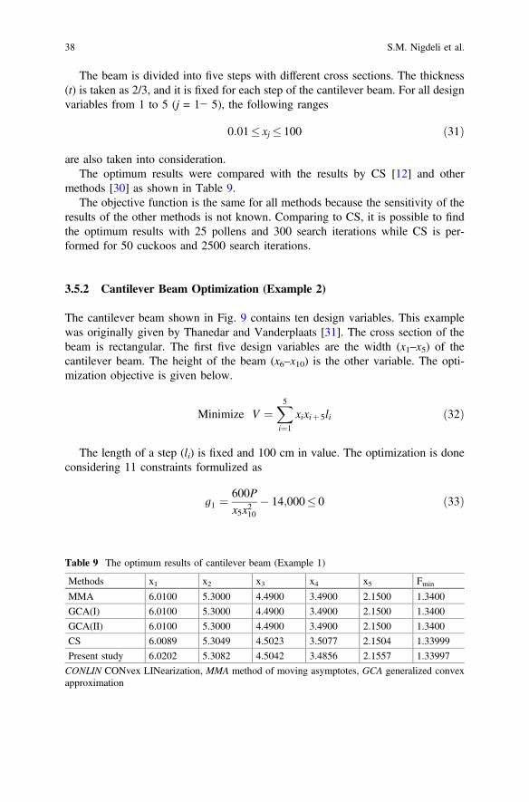
The beam is divided into five steps with different cross sections. The thickness(t) is taken as 2/3, and it is fixed for each step of the cantilever beam. For all designvariables from 1 to 5 (j = 1− 5), the following ranges

0:01� xj � 100 ð31Þ

are also taken into consideration.The optimum results were compared with the results by CS [12] and other

methods [30] as shown in Table 9.The objective function is the same for all methods because the sensitivity of the

results of the other methods is not known. Comparing to CS, it is possible to findthe optimum results with 25 pollens and 300 search iterations while CS is per-formed for 50 cuckoos and 2500 search iterations.

3.5.2 Cantilever Beam Optimization (Example 2)

The cantilever beam shown in Fig. 9 contains ten design variables. This examplewas originally given by Thanedar and Vanderplaats [31]. The cross section of thebeam is rectangular. The first five design variables are the width (x1–x5) of thecantilever beam. The height of the beam (x6–x10) is the other variable. The opti-mization objective is given below.

Minimize V ¼X5i¼1

xixiþ 5li ð32Þ

The length of a step (li) is fixed and 100 cm in value. The optimization is doneconsidering 11 constraints formulized as

g1 ¼600Px5x210

� 14;000� 0 ð33Þ

Table 9 The optimum results of cantilever beam (Example 1)

Methods x1 x2 x3 x4 x5 Fmin

MMA 6.0100 5.3000 4.4900 3.4900 2.1500 1.3400

GCA(I) 6.0100 5.3000 4.4900 3.4900 2.1500 1.3400

GCA(II) 6.0100 5.3000 4.4900 3.4900 2.1500 1.3400

CS 6.0089 5.3049 4.5023 3.5077 2.1504 1.33999

Present study 6.0202 5.3082 4.5042 3.4856 2.1557 1.33997

CONLIN CONvex LINearization, MMA method of moving asymptotes, GCA generalized convexapproximation

38 S.M. Nigdeli et al.

g2 ¼6Pðls þ l4Þ

x4x29� 14;000� 0 ð34Þ

g3 ¼6Pðls þ l4 þ l3Þ

x3x28� 14;000� 0 ð35Þ

g4 ¼6Pðls þ l4 þ l3 þ l2Þ

x2x27� 14;000� 0 ð36Þ

g5 ¼6Pðls þ l4 þ l3 þ l2 þ l1Þ

x1x26� 14;000� 0 ð37Þ

g6 ¼Pl3

3E1Isþ 7

I4þ 19

I3þ 37

I2þ 61

I1

� 2:7� 0 ð38Þ

g7 ¼x10x5

� 20� 0 ð39Þ

g8 ¼x9x4

� 20� 0 ð40Þ

g9 ¼x8x3

� 20� 0 ð41Þ

g10 ¼x7x2

� 20� 0 ð42Þ

g11 ¼x6x1

� 20� 0 ð43Þ

The solution range ares

1� xi � 5 for i ¼ 1 to 5 ð44Þ

and

30� xi � 65 for i ¼ 1 to 5 ð45Þ

In addition, P = 50,000 kN and E = 2 × 107 N/cm2. The optimum results arepresented in Table 10. The FPA algorithm is effective to find the minimumobjective function value of the numerical example.

Application of the Flower Pollination Algorithm … 39

4 Conclusion

From the extensive discussions in this chapter, it can be concluded that the FPA isan effective and suitable algorithm for solving structural engineering problems. It isalso easy to implement.

For the pin-jointed plane frame optimization problem, the best optimum resultshave been obtained by FPA comparing to GA [20] and CS [12]. In addition, theproblem has been solved for different loads. As the load increases, the objectivefunction (total length of bars) also increases.

The optimization results of three-bar truss system by the FPA have also beencompared with the results by CS [12], bat algorithm [14], and several other methods[22–24]. The results of FPA are slightly better than the results of other methodswithout exceeding the design constraints.

For the third example, the vertical deflection of an I-beam has been minimized.An important reduction of the existing best results is not provided, but similarresults were obtained with a slight improvement using FPA. The major advantage isthe shorter computation time and the robustness of the method because the optimumresults were obtained for a much lower number of function evaluations than that inCS [13].

The tubular column design under a compressive load is a major structuralengineering problem. The results for this example have been compared with theresults by CS [12] and several other approaches. The results obtained by FPA aremore effective than others.

The last examples are about two types of cantilever beams and the weightoptimization of structural elements has been carried out. Comparing with other

Table 10 The optimum results of cantilever beam (Example 2)

Thanedar andVanderplaats[31]

Lamberti andPappalettere[32]

HuangandArora[33]

BA [14] Presentstudy

x1 3.06 – – 2.99204 2.98211

x2 2.81 – – 2.77756 2.77002

x3 2.52 – – 2.52359 2.51546

x4 2.2 – – 2.20455 2.19861

x5 1.75 – – 1.74977 1.74722

x6 61.16 – – 59.84087 59.94777

x7 56.24 – – 55.55126 55.6512

x8 50.47 – – 50.4718 50.58328

x9 44.09 – – 44.09106 44.17907

x10 35.03 – – 34.99537 35.02744

Bestobjective

63110 65352.2 63108.7 61914.9 61849.9

40 S.M. Nigdeli et al.

methods, the improvement of the result is not physically meaningful for the firstcantilever beam example; however, the results are obtained after a much lowernumber of iterations comparing with those in CS [12]. For the second cantileverbeam example with 10 variables and 11 constraints, FPA is very effective and hasobtained much better results.

All the above confirm that FPA is a feasible algorithm for optimization instructural engineering by providing better designs with less computing time andimproving the robustness of finding the best optimum values. The effectiveness ofFPA can be attributed to the fact that it is a good combination of local search(self-pollination) and global search (cross-pollinations). It can be expected that FPAcan be used to solve many other optimization problems.

References

1. Yang, X.S.: Nature-Inspired Metaheuristic Algorithms. Luniver Press (2008)2. Yang, X.S.: Engineering Optimization: An Introduction with Metaheuristic Applications.

Wiley, New York (2010)3. Goldberg, D.E.: Genetic Algorithms in Search, Optimization and Machine Learning. Addison

Wesley, Boston (1989)4. Holland, J.H.: Adaptation in Natural and Artificial Systems. University of Michigan Press,

Ann Arbor (1975)5. Kirkpatrick, S., Gelatt, C., Vecchi, M.: Optimization by simulated annealing. Science 220,

671–680 (1983)6. Dorigo, M., Maniezzo, V., Colorni, A.: The ant system: optimization by a colony of

cooperating agents. IEEE Trans. Syst. Man Cybern. B 26, 29–41 (1996)7. Nakrani, S., Tovey, C.: On honey bees and dynamic allocation in an internet server colony.

Adapt. Behav. 12(3–4), 223–240 (2004)8. Kennedy, J., Eberhart, R.C.: Particle swarm optimization. In: Proceedings of IEEE

International Conference on Neural Networks No. IV, 27 Nov–1 Dec, pp. 1942–1948,Perth Australia (1995)

9. Glover, F.: Heuristic for integer programming using surrogate constraints. Decis. Sci. 8, 156–166 (1977)

10. Geem, Z.W., Kim, J.H., Loganathan, G.V.: A new heuristic optimization algorithm: harmonysearch. Simulation 76, 60–68 (2001)

11. Erol, O.K., Eksin, I.: A new optimization method: big bang big crunch. Adv. Eng. Softw. 37,106–111 (2006)

12. Gandomi, A.H., Yang, X.S., Alavi, A.H.: Cuckoo search algorithm: a metaheuristic approachto solve structural optimization problems. Eng. Comput. 29, 17–35 (2013)

13. Kaveh, A., Talatahari, A.: A novel heuristic optimization method: charged system search. ActaMech. 213, 267–289 (2010)

14. Yang, X.S., Gandomi, A.H.: Bat algorithm: a novel approach for global engineeringoptimization. Eng. Comput. 29(5), 464–483 (2012)

15. Yang, X.S., Deb, S.: Two-stage eagle strategy with differential evolution. Int. J. Bio-InspiredComput. 4(1), 1–5 (2012)

16. Yang, X.S.: Flower pollination algorithm for global optimization. In: UnconventionalComputation and Natural Computation 2012. Lecture Notes in Computer Science, vol. 7445,pp. 240–249 (2012)

Application of the Flower Pollination Algorithm … 41

17. Kaveh, A., Khayatazad, M.: A novel meta-heuristic method: ray optimization. Comput. Struct.112–113, 283–294 (2012)

18. Yang, X.S., Karamanoglu, M., He, X.: Flower pollination algorithm: a novel approach formultiobjective optimization. Eng. Optim. 46(9), 1222–1237 (2012)

19. Majid, K.I.: Optimum design of structures. Newnes-Butterworth, London (1974)20. Li, J.P., Balazs, M.E., Parks, G.T.: Engineering design optimization using species-conserving

genetic algorithms. Eng. Optm. 39(2), 147–161 (2007)21. Nowcki, H.: Optimization in pre-contract ship design. In: Fujita, Y., Lind, K., Williams, T.

J. (eds.) Computer Applications in the Automation of Shipyard Operation and Ship Design,vol. 2, pp. 327–338. Elsevier, New York (1974)

22. Park, Y.C., Chang, M.H., Lee, T.Y.: A new deterministic global optimization method forgeneral twice differentiable constrained nonlinear programming problems. Eng. Optim. 39(4),397–411 (2007)

23. Ray, T., Saini, P.: Engineering design optimization using a swarm with an intelligentinformation sharing among individuals. Eng. Optm. 33(6), 735–748 (2001)

24. Tsai, J.: Global optimization of nonlinear fractional programming problems in engineeringdesign. Eng. Optim. 37(4), 399–409 (2005)

25. Gold, S., Krishnamurty, S.: Trade-offs in robust engineering design. In: Proceedings of the1997 ASME Design Engineering Technical Conferences, DETC97/DAC3757, 14–17 Sept,Saramento, California (1997)

26. Wang, G.G.: Adaptive response surface method using inherited latin hypercube design points.Trans. ASME 125, 210–220 (2003)

27. Hsu, Y.L., Liu, T.C.: Developing a fuzzy proportionalderivative controller optimizationengine for engineering design optimization problems. Eng. Optm. 39(6), 679–700 (2007)

28. Rao, S.S.: Engineering optimization: theory and practice, 3rd edn. Wiley, Chichester (1996)29. Fleury, C., Braibant, V.: Structural optimization: a new dual method using mixed variables.

Int. J. Numer. Meth. Eng. 23, 409–428 (1986)30. Chickermane, H., Gea, H.C.: Structural optimization using a new local approximation method.

Int. J. Numer. Meth. Eng. 39, 829–846 (1996)31. Thanedar, P.B., Vanderplaats, G.N.: Survey of discrete variable optimization for structural

design. J. Struct. Eng. ASCE 121(2), 301–306 (1995)32. Lamberti, L., Pappalettere, C.: Move limits definition in structural optimization with sequential

linear programming. Part II Numer. Ex. Comput. Struct. 81, 215–238 (2003)33. Huang, M.W., Arora, J.S.: Optimal design with discrete variables: some numerical

experiments. Int. J. Numer. Meth. Eng. 40, 165–188 (1997)

42 S.M. Nigdeli et al.

Use of Swarm Intelligence in StructuralSteel Design Optimization

Mehmet Polat Saka, Serdar Carbas, Ibrahim Aydogduand Alper Akin

Abstract In this chapter, the optimum design problem of steel space frames isformulated according to the provisions of LRFD-AISC (Load and Resistance FactorDesign-American Institute of Steel Corporation). The weight of the steel frame istaken as the objective function to be minimized. The design optimization problemnecessitates selection of steel sections for the members of the steel frame from theavailable steel profiles lists. This turns the design optimization problem into discreteprogramming problem. Obtaining the optimum solution of such programmingproblems is cumbersome with mathematical programming techniques. On the otherhand with the use of recently developed metaheuristic techniques that are based onswarm intelligence, the solution of the same problem becomes straightforward. Fivedifferent structural optimization algorithms are developed which are based on antcolony optimization, particle swarm optimizer, artificial bee colony algorithm,firefly algorithm, and cuckoo search algorithm, respectively. Two real size steelspace frames; one rigidly connected and the other pin jointed are designed usingeach of these algorithms. The optimum designs obtained by these techniques arecompared and performance of each version is evaluated. It is noticed that most ofswarm intelligence-based algorithms are simple and robust techniques that deter-mine the optimum solution of structural design optimization problems efficientlywithout requiring much of a mathematical struggle.

M.P. Saka (&)Department of Civil Engineering, University of Bahrain, Isa Town, Bahraine-mail: mpsaka@uob.edu.bh

S. CarbasDepartment of Civil Engineering, Karamanoglu Mehmetbey University, Karaman, Turkeye-mail: scarbas@kmu.edu.tr

I. AydogduDepartment of Civil Engineering, Akdeniz University, Antalya, Turkeye-mail: aydogdu@akdeniz.edu.tr

A. AkinThomas & Betts Corporation, Meyer Steel Structures, Memphis, TN 38125, USAe-mail: alperakin@yahoo.com

© Springer International Publishing Switzerland 2016X.-S. Yang et al. (eds.), Metaheuristics and Optimization in Civil Engineering,Modeling and Optimization in Science and Technologies 7,DOI 10.1007/978-3-319-26245-1_3

43

Keywords Structural design optimization � Load and resistance factor design(LRFD) � Swarm intelligence � Ant colony algorithm � Particle swam optimizer �Artificial bee colony algorithm � Firefly algorithm � Cuckoo search algorithm

1 Introduction

Competitiveness of today’s economy and diminishing of world’s limited resourcesare forcing structural designers to come up with structures that require just sufficientmaterial to be built, while its response to external loads is within design codelimitations. Undoubtedly, excessive use of materials in structural design not onlyyields expensive structures that cause constructors to loose tenders but also con-sumes more of natural sources and adds more pollution to the atmosphere whichtriggers global warming. Hence, it is apparent that in order to have a sustainabledevelopment, structures are required to be designed and built using sufficientamount of material but not more. Structural design optimization tools exactly try toachieve this goal. They aim to design steel structures such that the steel frames havethe minimum weight (minimum material) and in the meantime the response of theframe under the external loads that the frame may be subjected to during its lifetimeis within the design code limitations. Design of steel structures has its own featuresand not similar to the design of other structures. Designer cannot use any sectionshe/he may desire but to select among the set of steel profiles available in practicefor beams and columns of the frame under consideration. This selection is requiredto be carried out in such a way that the frame with the selected steel profiles shouldhave the displacements less than those prescribed in the design code and itsmembers have sufficient strength to satisfy the design strength limitations under theexternal loads as described in steel design code provisions. In the meantime, it is thedesire of structural designer that the cost of the structure is the minimum.

In this chapter, first the design optimization problem of steel space framesaccording to the provisions of LRFD-AISC (Load and Resistance factor Design—American Institution of Steel Corporation) [1] is presented. The aim of the optimumdesign is to minimize the weight of the steel frame which becomes the objectivefunction in the programming problem. The objective function and the designconstraints as given by LRFD-AISC are described in detail in the following sec-tions. It should be noticed that structural steel design in practice requires selectionof steel profiles from the available steel profile list for the members of the steelframe under consideration for design. Therefore, the structural steel design opti-mization problem requires finding out the steel profile designations from theavailable set of steel sections for the members of a steel frame such that with thesesteel sections the weight of the steel frame is the minimum and its behavior underthe external loads within the limitations described in steel design code.

44 M.P. Saka et al.

The mathematical model of such optimization problem turns out to be anonlinear discrete programming problem. Among the mathematical programmingtechniques available to obtain the solution of such discrete variables, problem issequential linear discrete programming algorithm [2]. This technique attempts toobtain the solution of nonlinear discrete programming problem by solving series ofmixed-integer linear programming problems. The nonlinear problems are linearizedabout an initially selected point using first-order Taylor’s series expansion.However, because of the discrete variables the mixed-integer linear programmingtechnique cannot be applied directly. The discrete variables are to be redefined bymeans of another set of design variables where the new design variables are to beequal either zero or one in the solution. These additional design variables increasethe total number of variables in the problem needlessly which makes the coding ofthe algorithm quite cumbersome. The success of obtaining the optimum solution isclosely related with the quality of the selection of the initial design point.Furthermore, computational difficulties such as convergence problems can bestumbled in large size optimization problems.

The metaheuristic techniques that are emerged in last three decades do not sufferthe above discrepancies [3–10]. They are nontraditional stochastic search andoptimization methods that quite effective in finding the optimum solution ofcombinatorial optimization problems similar to the one described in the precedingsection. They do not require the gradient information of the objective function andconstraints and they use probabilistic transition rules not deterministic rules. Thesemethods move within a design domain randomly with the aim of reaching theoptimum solution. However, this random move is not based on a blind way ofsearching for the optimum in a confined design region but it makes use of anintelligent heuristics to guide the search. This is why stochastic search methods arealso called metaheuristic algorithms. The fundamental properties of metaheuristicalgorithms are that they imitate certain strategies taken from nature, social culture,biology, or laws of physics that direct the search process. The strategies employedin search of optimum solution in these techniques simulate the natural phenomena.Among the metaheuristic algorithms, those who are based on swarm intelligenceare shown to be robust, effective, and quite powerful techniques in obtaining nearoptimum solutions if not optimum in engineering design optimization problems[10]. There are several reviews available in the literature which comprehensivelysummarizes the use of metaheuristic algorithms in the design optimization of steelskeletal structures [11–16].

In this chapter, five different structural design optimization algorithms aredeveloped which are based on ant colony optimization, particle swarm optimizer,artificial bee colony algorithm, firefly algorithm, and cuckoo search algorithm,respectively. Two real size steel space frames are designed using each of thesealgorithms considering the LRFD-AISC provisions. The optimum designs obtainedby these techniques are compared and performance of each version is evaluated.

Use of Swarm Intelligence in Structural Steel Design Optimization 45

2 Discrete Optimum Design of Steel Space Framesto LRFD-AISC

The design of steel space frames necessitates the selection of steel sections for itscolumns and beams from standard steel section tables such that the frame satisfiesthe serviceability and strength requirements specified by the code of practice whilethe economy is observed in the overall or material cost of the frame. When thedesign constraints are implemented from LRFD-AISC, the following nonlineardiscrete programming problem is obtained.

2.1 The Objective Function

The objective function is taken as the minimum weight of the frame which isexpressed as follows:

Minimize W ¼Xng

r¼1mr

Xtrs¼1

‘s ð1Þ

where W defines the weight of the frame, mr is the unit weight of the steel sectionselected from the standard steel sections table that is to be adopted for group r, tr isthe total number of members in group r, ng is the total number of groups in theframe, and ls is the length of members which belongs to group r.

2.2 Strength Constraints

For the case where the effect of warping is not included in the computation of thestrength capacity of W sections that are selected for beam–column members of theframe, the following inequalities given in Chapter H of LRFD-AISC are required tobe satisfied:

forPu

/Pn� 0:2; gs;i ¼ Pu

/Pnþ 8

9Mu

/bMnxþ Mu

/bMny

� �� 1; 0 ð2Þ

forPu

uPn\0:2; gs;i ¼ Pu

2/ Pnþ Mu

/bMnxþ Mu

/bMny

� �� 1; 0 ð3Þ

46 M.P. Saka et al.

whereMnx is the nominal flexural strength at strong axis (x axis),Mny is the nominalflexural strength at weak axis (y axis), Mux is the required flexural strength at strongaxis (x axis), Muy is the required flexural strength at weak axis (y axis), Pn is thenominal axial strength (tension or compression), and Pu is the required axialstrength (tension or compression) for member i and ‘ represents the loading case.The values of Mux and Muy are required to be obtained by carrying out P� Danalysis of the steel frame. This is an iterative process which is quite time con-suming. In Chapter C of LRFD-AISC, an alternative procedure is suggested for thecomputations of Mux and Muy values. In this procedure, two first-order elasticanalyses are carried out. In the first, frame is analyzed under the gravity loads onlywhere the sway of the frame is prevented to obtain Mnt values. In the second, theframe is analyzed only under the lateral loads to find Mlt values. These momentvalues are then combined using the following equation as given in the design code:

Mu ¼ B1Mnt þB2Mlt ð4Þ

where B1 is the moment magnifier coefficient and B2 is the sway moment magnifiercoefficient. The details of how these coefficients are calculated are given inChapter C of LRFD-AISC [1]. Equations (2) and (3) represent strength constraintsfor doubly and singly symmetric steel members subjected to axial force andbending. If the axial force in member k is tensile force, the terms in these equationsare given as follows: Puk is the required axial tensile strength, Pnk is the nominaltensile strength, / becomes /t in the case of tension and called strength reductionfactor which is given as 0.90 for yielding in the gross section and 0.75 for fracturein the net section, /b is the strength reduction factor for flexure given as 0.90, Muxk

and Muyk are the required flexural strength, and Mnxk and Mnyk are the nominalflexural strengths about major and minor axis of member k, respectively. It shouldbe pointed out that required flexural bending moment should include second-ordereffects. LRFD suggests an approximate procedure for computation of such effectswhich is explained in C1 of LRFD. In the case the axial force in member k iscompressive force, the terms in Eqs. (2) and (3) are defined as follows: Puk is therequired compressive strength, Pnk is the nominal compressive strength, and /becomes /c which is the resistance factor for compression given as 0.85. Theremaining notations in Eqs. (2) and (3) are the same as the definition given above.

The nominal tensile strength of member k for yielding in the gross section iscomputed as Pnk ¼ FyAgk where Fy is the specified yield stress and Agk is the grossarea of member k. The nominal compressive strength of member k is computed as

Pnk ¼ AgkFcr where Fcr ¼ 0:658k2c

� �Fy for kc� 1:5 and Fcr ¼ 0:877=k2c

� �Fy for

kc [ 1:5 and kc ¼ Klrp

ffiffiffiffiffiffiffiffiffiffiffiFyE

q. In these expressions, E is the modulus of elasticity,

and K and l are the effective length factor and the laterally unbraced length ofmember k, respectively.

Use of Swarm Intelligence in Structural Steel Design Optimization 47

2.3 Displacement Constraints

The lateral displacements and deflection of beams in steel frames are limited by thesteel design codes due to serviceability requirements. According to the ASCE AdHoc Committee report [17], the accepted range of drift limits in the first-orderanalysis is 1/750–1/250 times the building height H with a recommended value ofH/400. The typical limits on the inter-story drift are 1/500–1/200 times the storyheight. Based on this report, the deflection limits recommended are proposed in[18–20] for general use which is repeated in Table 1.

2.3.1 Deflection Constraints

It is necessary to limit the mid-span deflections of beams in a steel space frame notto cause cracks in brittle finishes that they may support due to excessive dis-placements. Deflection constraints can be expressed as an inequality limitation asshown in the following:

gdj ¼ djlduj� 1� 0 j ¼ 1; . . .; nsm ; l ¼ 1; . . .; nlc ð5Þ

where djl is the maximum deflection of jth member under the lth load case, duj is theupper bound on this deflection which is defined in the code as span/360 for beamscarrying brittle finishers, nsm is the total number of members where deflectionslimitations are to be imposed, and nlc is the number of load cases.

2.3.2 Drift Constraints

These constraints are of two types. One is the restriction applied to the top storysway and the other is the limitation applied on the inter-story drift.

Top Story Drift ConstraintTop story drift limitation can be expressed as an inequality constraint as shown inthe following:

Table 1 Displacement limitations for steel frames

Item Deflection limit

1 Floor girder deflection for service live load L/360

2 Roof girder deflection L/240

3 Lateral drift for service wind load H/400

4 Inter-story drift for service wind load H/300

48 M.P. Saka et al.

gtdj ¼Dtop� �

jl

H=Ratio� 1� 0 j ¼ 1; . . .; njtop; l ¼ 1; . . .; nk ð6Þ

where H is the height of the frame, njtop is the number of joints on the top story, nlcis the number of load cases, and Dtop

� �jl is the top story drift of the jth joint under

lth load case.

Inter-Story DriftIn multi-story steel frames, the relative lateral displacements of each floor arerequired to be limited. This limit is defined as the maximum inter-story drift whichis specified as hsx/Ratio where hsx is the story height and ratio is a constant valuegiven in ASCE Ad Hoc Committee report [14].

gidj ¼Dohð Þjl

hsx=Ratio� 1� 0 j ¼ 1; . . .; nst; l ¼ 1; . . .; nlc ð7Þ

where nst is the number of story, nlc is the number of load cases, and Dohð Þjl is thestory drift of the jth story under lth load case.

2.4 Geometric Constraints

In steel frames, it is desired that column section for upper floor should not have alarger section than the lower story column for practical reasons, because having alarger section for upper floor requires a special joint arrangement which is neitherpreferred nor economical. The same applies to the beam-to-column connections.The W section selected for any beam should have a flange width smaller than orequal to the flange width of the W section selected for the column to which thebeam is to be connected. These are shown in Fig. 1 and named as geometricconstraints. These limitations are included in the design optimization model tosatisfy practical requirements. Two types of geometric constraints are considered inthe mathematical model. These are column-to-column geometric constraints andbeam-to-column geometric limitations.

2.4.1 Column-to-Column Geometric Constraints

The depth and the unit weight of W sections selected for the columns of twoconsecutive stores should be either equal to each other or the one in the upper storyshould be smaller than the one in the lower story. These limitations are included inthe design problem as inequality constraints as shown in the following:

Use of Swarm Intelligence in Structural Steel Design Optimization 49

gcdi ¼ Di

Di�1� 1� 0 i ¼ 2. . .nj ð8Þ

gcmi ¼ mi

mi�1� 1� 0 i ¼ 2. . .nj ð9Þ

where nj is the number of stories, mi is the unit weight of W section selected forcolumn story i, mi�1 is the unit weight of W section selected for of column story(i − 1), Di is the depth of W section selected for of column story i, and Di�1 is thedepth of W section selected for of column story (i − 1).

2.4.2 Beam-to-Column Geometric Constraints

When a beam is connected to a flange of a column, the flange width of the beamshould be less than or equal to the flange width of the column so that the connectioncan be made without difficulty. In order to achieve this, the flange width of thebeam should be less than or equal to D� 2tbð Þ of the column web dimensions in theconnection where D and tb are the depth and the flange thickness of W section,respectively, as shown in Fig. 1:

gbci ¼Bf� �

bi

Dci � 2 tbcð Þi� 1� 0 i ¼ 1. . .nj1 ð10Þ

Fig. 1 Beam columngeometric constraints

50 M.P. Saka et al.

or

gbbi ¼Bf� �

bi

Bf� �

ci

� 1� 0 i ¼ 1. . .nj2 ð11Þ

where nj1 is the total number of joints where beams are connected to the web of acolumn, nj2 is the total number of joints where beams connected to the flange of acolumn, Dci is the depth of W section selected for the column at joint i, tbð Þcj is theflange thickness of W section selected for the column at joint i, Bf

� �ci is the flange

width of W section selected for the column at joint i, and Bf� �

bi is the flange widthof W section selected for the beam at joint i.

The optimum design of steel space frames problem described in precedingsections where the objective function is given in Eq. (1) and the constraints aredepicted from Eq. (2) to (11) is a nonlinear discrete optimization problem. It isapparent that in order to determine the optimum solution of this problem steeldesigner has to find out the suitable combination of W sections that makes theframe weight minimum and in the same time the design code provisions are allsatisfied. Here the selection of a W section from an available steel profile list iscarried out by choosing an integer number from a set which consists of integernumbers starting from 1 to the total number of sections in the list. This integernumber is the sequence number of that particular W section. Hence, the designsolution is a set of integer numbers each of which represents the sequence numberof W section in the design pool. This is a combinatorial optimization problem.

3 Swarm Intelligence-Based Metaheuristic OptimizationAlgorithms

Metaheuristic optimization algorithms differ from that of mathematical program-ming techniques in the fact that they do not employ gradient descent orquasi-Newton techniques but heuristic search. A heuristic exploitsproblem-depended information to find a sufficiently good solution to a specificproblem, while metaheuristic is a general-purpose algorithm that can be appliedalmost any type of optimization problem. In reality, metaheuristic is also heuristic,but a more powerful one that can be viewed as upper level general method with aguiding strategy in designing underlying heuristic. The rule of thumb selected forexploration of the optimum solution by metaheuristic algorithms may be borrowedfrom nature or social culture. In general, a metaheuristic is an iterative process withset of concepts that are used for exploring and exploiting the search space todetermine the best solution among the alternative solutions. Metaheuristic algo-rithms are not problem specific, approximate, and usually non-deterministic. It isimportant that there should be a dynamic balance between diversification andintensification in metaheuristic procedure. Diversification generally refers to the

Use of Swarm Intelligence in Structural Steel Design Optimization 51

exploration of the search space and intensification refers to the exploitation of theaccumulated search experience. The balance between these two concepts isimportant so as not to waste too much time in regions of the search space whichdoes not possess high-quality solutions while the algorithm can quickly find out theregions of high-quality solutions [3–10].

Some of the recent metaheuristic techniques are based on swarm intelligence.A swarm is a large number of homogenous, unsophisticated agents that interactlocally among themselves, and their environment, without any central control ormanagement to yield a global behavior to emerge. Biologists are amazed with forexample what an ant or bee colony achieves. Although single ant or a bee is notsmart individual, their colonies are smart. When it comes to deciding what to donext, most ants or bees do not have any clue. However, as a swarm, they can findthe shortest route to the best food source, allocate workers to different tasks, anddefend a territory from invaders without having someone in control or as manager.As an individual they are tiny dummies, but they respond quickly and effectively totheir environment as colonies. This is what is called swarm intelligence [10]. It isthe collective behavior of decentralized and self-organized natural or artificialsystems. Metaheuristic optimization techniques based on swarm intelligence aremade up population of simple agents interacting with one another and with theirenvironment as is the case in ant colonies, bird flocking, animal herding, and fishschooling. These techniques imitate the behavior of these colonies in a numericaloptimization procedure. They employ what for example an ant colony uses to findthe shortest route between their nest and food source as a guiding mechanism inorder to search design domain to find the optimum solution of an optimizationproblem. They also utilize some additional strategies to avoid getting trapped inconfined areas of search domain. Latest applications have shown that they arerobust, effective, and quite powerful in obtaining near optimum solutions if notoptimum in engineering design optimization problems [3, 10].

Performance evaluation of different metaheuristic algorithms in structural steeldesign optimization is carried out in the literature [21, 22]. This chapter intends toexamine the use of swarm intelligence-based structural design optimization algo-rithms. For this purpose, five structural design optimization algorithms are developedeach of which based on ant colony algorithm, particle swarm optimizer, artificial beecolony algorithm, firefly algorithm, and cuckoo search algorithm. Ant colony algo-rithm is inspired from the way that ant colonies find the shortest route between thefood source and their nest [23–25]. Particle swarm optimizer mimics the socialbehavior of bird flocking [26, 27]. Artificial bee colony algorithm imitates the for-aging behavior of honey bee colony [28, 29]. Firefly algorithm imitates the idealizedbehavior offlashing characteristics offireflies. These insects communicate, search forpray, and find mates using bioluminescence with varying flaying patterns [30–32].Cuckoo search algorithm simulates reproduction strategy of cuckoo birds [33].

Some of the optimization problems do not have any constraints and they onlyrequire minimizing or maximizing the objective function. However, most of theoptimization problems in practice do have constraints. Swarm intelligence-basedalgorithms can only handle unconstrained optimization problems. Hence, it

52 M.P. Saka et al.

becomes necessary to transform the optimization problem with constraints into theone which is unconstrained. This is achieved by either using a penalty function.There are several penalty function methods. Very comprehensive review of thesetechniques is covered [34]. One of the commonly used penalty functions is given inthe following:

Wp ¼ W 1þCð Þe ð12Þ

where W is the value of objective function of optimum design problem given inEq. (1), Wp is the penalized weight of structure, C is the value of total constraintviolations which is calculated by summing the violation of each individual con-straint, and ε is penalty coefficient which is taken as 2.0 in this work as suggested in[21, 22].

c ¼Xnci¼1

ci ð13Þ

ci ¼ 0 if gj� 0gj if gj [ 0

j ¼ 1; . . .; nc ð14Þ

where gj is the jth constraint function and nc is the total number of constraints in theoptimum design problem. Constraint functions for the steel frame are given throughin Eqs. (2)–(11). It should be reminded that all the constraints are required to benormalized before they are used in the metaheuristic algorithms. A solution vectorwhichmay be slightly infeasible in one ormore constraints is also included among thefeasible solutions. This is called adaptive error strategy which is explained in [35].

3.1 Ant Colony Optimization (ACO)

Ant colony optimization technique is inspired from the way that ant colonies findthe shortest route between the food source and their nest. Ants being completelyblind individuals can successfully discover as a colony the shortest path betweentheir nest and the food source. They manage this through their typical characteristicof employing volatile substance called pheromones. They perceive these substancesthrough very sensitive receivers located in their antennas. The ants deposit pher-omones on the ground when they travel which is used as a trail by other ants in thecolony. When there is choice of selection for an ant between two paths, it selects theone where the concentration of pheromone is more. Since the shorter trail will bereinforced more than the long one after a while a great majority of ants in the colonywill travel on this route. Ant colony optimization algorithm is first used in findingthe solution of traveling salesman [23–25]. The steps of ant colony optimization areas follows:

Use of Swarm Intelligence in Structural Steel Design Optimization 53

1. Select number of ants each of which represents a potential solution to theoptimization problem. Define a pool for each decision variable in the opti-mization problem which consists of possible values that particular variable cantake. Assign randomly each ant to each decision variable. Calculate initialpheromone amount (s0) as s0 ¼ 1=Zmin where Zmin is the minimum value of theobjective function without penalty violation. The pheromone and visibilityvalues for each decision variable are calculated defined as given below:

sij ¼ 1s0

; vij ¼ 1xij

; i ¼ 1; 2; . . .; nv j ¼ 1; 2; . . .; npool ð15Þ

where xij is jth value of the design variable i, nv is the total number of designvariables in the optimization problem, and npool is the total number of values inthe pool from which a value can be selected for decision variable i.

2. Each ant in the colony selects its first design variables. Ants then select valuesfor their decision variables from the value pool. This selection is carried out by adecision process which depends on probability computation given below:

Pij tð Þ ¼sijðtÞ� �a� vij

� �bPndiv

j2allowed sijðtÞ� �a� vij

� �b i ¼ 1; 2; . . .; nv j ¼ 1; 2; . . .; npool ð16Þ

where Pij tð Þ is the probability of jth value selected from the pool for decisionvariable i which is assigned to ant at time t. a and b are the parameters which areused to arrange the influence of local trail values and visibility, respectively.This process continues until all ants assign values for their first design variables.

3. Apply local update rule at the end of the each tour. Concentration of pheromonefor values selected by ants from the pool is lowered in order to promoteexploration in the search. This corresponds to the evaporation of the pheromonesubstance in the real life. The mathematical expression for this is sij tð Þ ¼f � sijðtÞ where f is called local update coefficient whose value changes from 0 to1. If the value of this parameter is selected close to 1, fast convergence occursand the algorithm may end up with a local optimum. On the other hand, if thevalue is chosen close to 0 convergence difficulties arise in the problem.

4. Start assigning a value from the pool for the next decision variable. Continuethis assigning procedure until all the ants in the colony have a value for eachdecision variable. At the end of the tour, apply local update rule. This procedurecontinues until all ants assign values for all decision variables. At the end of thisprocess, each ant has a selected value for each decision variable and all togethereach ant represents a candidate solution for the optimization problem.

54 M.P. Saka et al.

5. Apply global update scheme using Eq. (17):

sij tþ nð Þ ¼ q � sij tð ÞþDsij tð Þ ð17Þ

where q is constant selected between 0 and 1. 1� qð Þ represents the evaporationamount of pheromone between time t and tþ n (the amount of time required tocomplete a cycle). Dsij is the change in pheromone amount on the pathconnecting decision variable i to decision variable j. Value of Dsij is representedby the following formula:

Dsij ¼Xmk¼1

Dskij ð18Þ

where k represents any ant from 1 to m (where m is the number of ants) and Dskijis the change in the pheromone for ant k. Calculation of Dskij term is described asfollows:

Dskij ¼1Zk

ð19Þ

where Zk is the penalized objective function value for ant k. This is the end ofone ant colony algorithm cycle. To start another cycle, all ants are returned totheir initial decision variables and above steps are replicated again.

6. Repeat steps 2–5 until the termination criterion is satisfied which generally takenas the maximum number of iterations.

3.2 Particle Swarm Optimizer (PSO)

Particle swarm optimizer is based on the social behavior of animals such as fishschooling, insect swarming, and birds flocking [26, 27]. The method considers anartificial swarm which consists of particles (agents). The behavior of each agent inthe swarm is simulated according to three rules. The first is separation where eachagent tries to move away from its neighbors if they are too close. The second isalignment where each agent steers toward the average heading of its neighbors. Thethird is cohesion where each agent tries to go toward the average position of itsneighbors. This simulation is extended to have roost by [27]. They have amendedthe above three rules as follows: each agent is attracted toward the location of roost;each agent remembers where it was closer to the roost and each agent sharedinformation with all other agents about its closest location to the roost.

The particle swarm optimizer selects a number of particles to represent a swarm.Each particle in the swarm is a potential solution to the optimization problem underconsideration. A particle explores the search domain by moving around. This move isdecided by making use of its own experience and the collective experience of the

Use of Swarm Intelligence in Structural Steel Design Optimization 55

swarm. Each particle has three main parameters: position, velocity, and fitness.Position represents the decision variables of the optimization problem, velocitydetermines the rate of change of the position, and fitness is the value of the objectivefunction at the particle’s current position. Thefitness value is ameasure of howgood isthe solution it represents for the optimization problem. The algorithm starts solving anoptimization problem by first initializing each particle. In the initiation phase, eachparticle is given a random initial position and an initial velocity. The position of aparticle represents a solution of the problem and has therefore a value, given by theobjective function.While moving in the search space, particles memorize the positionof the best solution they found. At each iteration of the algorithm, each particle moveswith a velocity that is a weighted sum of three components: the old velocity, a velocitycomponent that drives the particle toward the location in the search space where itpreviously found the best solution so far, and a velocity component that drives theparticle towards the location in the search spacewhere the neighbor particles found thebest solution so far. There are several variants of particle swarmalgorithm.The steps ofthe standard algorithm are outlined in the following:

1. Initialize swarm of particles with positions xi0 and initial velocities vi0 randomlydistributed throughout the design space. These are obtained from the followingexpressions:

xi0 ¼ xminþ r xmax � xminð Þ ð20Þ

vi0 ¼ xminþ r xmax � xminð Þð Þ=Dt½ � ð21Þ

where the term r represents a random number between 0 and 1, and xmin andxmax represent the design variables upper and lower bounds, respectively.

2. Evaluate the objective function values f(xki ) using the design space positions xk

i .3. Update the optimum particle position pk

i at the current iteration k and the globaloptimum particle position pk

g.4. Update the position of each particle from xikþ 1 ¼ xik þ vikþ 1Dt where x

ikþ 1 is the

position of particle i at iteration k + 1, vikþ 1 is the corresponding velocity vector,and Dt is the time step value.

5. Update the velocity vector of each particle. There are several formulas for thisdepending on the particular particle swarm optimizer under consideration.

vikþ 1 ¼ wvik þ c1r1pik � xik� �

Dtþ c2r2

pgk � xik� �

Dtð22Þ

where r1 and r2 are the random numbers between 0 and 1, pik is the best positionfound by particle i so far, and pgk is the best position in the swarm at time k.w is theinertia of the particle which controls the exploration properties of the algorithm. c1and c2 are the trust parameters that indicate howmuch confidence the particle has initself and in the swarm, respectively. Usually, they are taken as 2.

56 M.P. Saka et al.

6. Repeat steps 2–5 until the stopping criterion is met.

In order to control the change of particles’ velocities, upper and lower bounds forthe velocity change are also limited to a user-specified value of vmax. Once the newposition of a particle is calculated, using Eq. (20), the particle then flies toward it.The main parameters used in the particle swarm optimizer are the population size(number of particles), number of generation cycles, and the maximal change of aparticle velocity of vmax.

3.3 Artificial Bee Colony Algorithm (ABC)

Artificial bee colony algorithmmimics the intelligent foragingbehavior of a honey beecolony [28]. In the artificial bee colony algorithm, there are three types of bees whichcarry out different tasks. The first group of bees is the employed bees that locate foodsource, evaluate its amount of nectar, and keep the location of better sources in theirmemory. These bees when fly back to hive share this information to other bees in thedancing area by dancing. The dancing time represents the amount of nectar in the foodsource. The second group is the onlooker beeswho observe the dance andmay decideto fly to the food source if they find it is worthwhile to visit the food source. Therefore,food sources reach in the amount of nectar attract more onlooker bees. The third groupis the scout bees that explore new food sources in the vicinity of the hive randomly. Theemployedbeewhose food sourcehas been abandonedby the bees becomes a scout bee.Overall, scout bees carry out the exploration, employed, andonlooker bees perform thetask of exploitation. Each food source is considered as a possible solution for theoptimization problem and the nectar amount of a food source represents the quality ofthe solution which is identified by its fitness value. The artificial bee colony algorithmconsists of four stages. These stages are initialization phase, employed bees phase,onlooker bees phase, and scout bees phase.

1. Initialization phase: Initialize all the vectors of the population of food sources,xp; p ¼ 1; . . .; np using Eq. (23) where np is the population size (total number ofartificial bees). Each food source is a solution vector consisting of n variablesðxpi; i ¼ 1; . . .; nÞ and it is a potential solution to the optimization problem underconsideration.

xpi ¼ xliþ randð0; 1Þðxui � xliÞ ð23Þ

where x‘i and xui are the upper and lower bounds on xi.2. Employed bees phase: Employed bees search new food sources using Eq. (24):

vpi ¼ xpiþ fpiðxpi � xkiÞ ð24Þ

where k 6¼ i is a randomly selected food source, and φpi is a random number inrange [−1, 1]. After producing the new food source, its fitness is calculated. If its

Use of Swarm Intelligence in Structural Steel Design Optimization 57

fitness is better than xpi the new food source replaces the previous one. Thefitness value of the food sources is calculated according to Eq. (25):

fitnessðxpÞ ¼1

1þ f ðxpÞ if f ðxpÞ� 01þ absðf ðxpÞÞ if f ðxpÞ\0

ð25Þ

3. Onlooker bees phase: Unemployed bees consist of two groups. These areonlooker bees and scouts. Employed bees share their food source informationwith onlooker bees. Onlooker bees choose their food source depending on theprobability value Pp which is calculated using the fitness values of each foodsource in the population as shown in Eq. (26):

Pp ¼ fitnessðxpÞPnpp¼1 fitnessðxpÞ

ð26Þ

After a food source xpi for an onlooker bee is probabilistically chosen, aneighborhood source is determined using Eq. (25) and its fitness value is computedusing Eq. (26).

4. Scout bees phase: The unemployed bees who choose their food sources ran-domly called scouts. Employed bees whose solutions cannot be improved afterpredetermined number of trials become scouts and their solutions are aban-doned. These scouts start to search for new solutions.

5. Phases 2–4 are repeated until the termination criterion is satisfied.

3.4 Firefly Algorithm (FFA)

Firefly algorithm is based on the idealized behavior of flashing characteristics offireflies [30, 31]. These insects communicate, search for pray, and find mates usingbioluminescence with varying flaying patterns. The firefly algorithm is based onthree rules, and they are as follows:

1. All fireflies are unisex so they attract one another.2. Attractiveness is propositional to firefly brightness. For any couple of flashing

fireflies, the less bright one moves toward the brighter one. Attractiveness isproportional to the brightness and they both decrease as their distance increases.If there is no brighter one than a particular firefly, it will move randomly.

3. The brightness of a firefly is affected or determined by the landscape of theobjective function.

Mathematical interpretation of the above rules is given in the following asexplained in [30].

Attractiveness: In the firefly algorithm, attractiveness of a firefly is assumed tobe determined by its brightness which is related with the objective function. The

58 M.P. Saka et al.

brightness i of a firefly at a particular location x can be chosen as IðxÞ / f ðxÞ wheref ðxÞ is the objective function. However, the attractiveness β is relative, and it shouldbe judged by the other fireflies. Thus, it will vary with the distance rij betweenfirefly i and firefly j. In the firefly algorithm, the attractiveness function is taken tobe proportional to the light intensity by adjacent fireflies and it is defined as follows:

bðrÞ ¼ b0e�c rm ; ðm� 1Þ ð27Þ

where b0 is the attractiveness at r ¼ 0.Distance: The distance between any two fireflies i and j at xi and xj is calculated

as

rij ¼ xi � xj�� �� ¼

ffiffiffiffiffiffiffiffiffiffiffiffiffiffiffiffiffiffiffiffiffiffiffiffiffiffiffiffiffiffiffiffiXdk¼1

xi;k � xj;k� �2

vuut ð28Þ

where xi;k is the kth component of the spatial coordinate xi of the ith firefly.Movement: The movement of a firefly i which is attracted to another brighter

firefly j is determined by

xi ¼ xiþ b0e�cr2ijðxj � xiÞþ a rand� 1

2

� �ð29Þ

where the second term is due to the attraction and the third term is the random-ization with α being the randomization parameter. “rand” is a random numbergenerator uniformly distributed in [0, 1].

The parameter αt essentially controls the randomness and to some extent, thediversity of solutions where t is the iteration number. This parameter can be tunedduring iterations so that it can vary with the iteration counter t. The expression ofαt = α0δ

t (0 < δ < 1) is suggested in [31] where α0 is the initial randomness scalingfactor, and δ is essentially a cooling factor. It is also stated in [31] that for mostapplications, the values from 0.95 to 0.97 is found suitable for δ. Regarding theinitial α0, simulations show that firefly algorithm is more efficient if α0 is associatedwith the scaling of design variables. Let L be the average scale of the problem ofinterest, and it is set as α0 = 0.01L initially. The factor 0.01 comes from the fact thatrandom walk requires a number of steps to reach the target while balancing the localexploitation without jumping too far in a few steps [31]. The parameter β controlsthe attractiveness, and parametric studies suggest that β0 = 1 can be used for mostapplications. However, it is mentioned in [31] that γ should be also related to thescaling L as γ = 1/√L.

The steps of the firefly algorithm are given below:

1. Generate initial population of n fireflies xif g; i ¼ 1; 2; . . .; nð Þ randomly each ofwhich represents a candidate solution to the optimization problem with objectivefunction of f ðxÞ and decision variables xf g ¼ x1; x2; . . .; xmf gT .

Use of Swarm Intelligence in Structural Steel Design Optimization 59

2. Compute light intensity using Eq. (27) for each firefly bf g ¼ b1; b2; . . .; bnf gT .The distance between fireflies is computed from Eq. (28).

3. Move each firefly i toward other brighter fireflies using Eq. (29). If there is otherbrighter firefly move it randomly.

4. Evaluate new solutions and update light intensity.5. Rank the fireflies and find the current best solution.6. Repeat steps 2–5 until the termination criterion is satisfied.

3.5 Cuckoo Search Algorithm (CSA)

Cuckoo search algorithm simulates reproduction strategy of cuckoo birds [33].Some species of cuckoo birds lay their eggs in the nests of other birds so that whenthe eggs are hatched their chicks are fed by the other birds. Sometimes, they evenremove existing eggs of host nest in order to give more probability of hatching oftheir own eggs. Some species of cuckoo birds are even specialized to mimic thepattern and color of the eggs of host birds so that host bird could not recognize theireggs which give more possibility of hatching. In spite of all these efforts to concealtheir eggs from the attention of host birds, there is a possibility that host bird maydiscover that the eggs are not its own. In such cases, the host bird either throwsthese alien eggs away or simply abandons its nest and builds a new nest somewhereelse. In cuckoo search algorithm, cuckoo egg represents a potential solution to thedesign problem which has a fitness value. The algorithm uses three idealized rulesas given in [33]. These are as follows: (a) each cuckoo lays one egg at a time anddumps it in a randomly selected nest. (b) The best nest with high-quality eggs willbe carried over to the next generation. (c) The number of available host nests isfixed and a host bird can discover an alien egg with a probability of Pa Є [0, 1]. Inthis case, the host bird can either throw the egg away or abandon the nest to build acompletely new nest in a new location.

Cuckoo search algorithm initially requires the selection of a population of n eggseach of which represents a potential solution to the design problem under consid-eration. This means that it is necessary to generate n solution vector of xf g ¼x1; x2; . . .; xmf gT in a design problem with m decision variables. For each potential

solution vector, the value of objective function f ðxÞ is also calculated. The algo-rithm then generates a new solution xmþ 1

i ¼ xmi þ bk for cuckoo i where xmþ 1i and

xmi are the previous and new solution vectors. β > 1 is the step size which is selectedaccording to the design problem under consideration. λ is the length of step sizewhich is determined according to random walk with Levy flights. A random walk isa stochastic process in which particles or waves travel along random trajectorieswhich consist of taking successive random steps. The search path of a foraginganimal can be modeled as random walk. A Levy flight is a random walk in whichthe steps are defined in terms of the step lengths which have a certain probability

60 M.P. Saka et al.

distribution, with the directions of the steps being isotropic and random. Hence,Levy flights necessitate selection of a random direction and generation of stepsunder chosen Levy distribution.

The algorithm given in [36] which is called Mantegna algorithm is one of thefast and accurate algorithms which generates a stochastic variable whose proba-bility density is close to Levy stable distribution characterized by arbitrary chosencontrol parameter α (0.3 ≤ α ≤ 1.99). Using the Mantegna algorithm, the step size λis calculated as

k ¼ x

yj j1=að30Þ

where x and y are the two normal stochastic variables with standard deviation σxand σy which are given as

rx að Þ ¼ C 1þ að Þ sin pa=2ð ÞC 1þ að Þ=2ð Þa2 a�1ð Þ=2

� 1=aand ryðaÞ ¼ 1 for a ¼ 1:5 ð31Þ

in which the capital Greek letter C represents the Gamma function

(CðzÞ ¼ R10tz�1e�zdt) that is the extension of the factorial function with its argument

shifted down by 1 to real and complex numbers. If z = k is a positive integerCðkÞ ¼ ðk � 1Þ!.

The steps of the cuckoo search algorithm are as follows:

1. Select values for cuckoo search algorithm parameters which are the number ofnests (eggs) (n), the step size parameter (β), discovering probability (pa), andmaximum number of iterations for termination of the cycles.

2. Generate initial population of n host nests xif g; i ¼ 1; 2; . . .; nð Þ randomly eachof which represents a candidate solution to the optimization problem withobjective function of f(x) and decision variables xf g ¼ x1; x2; . . .; xmf gT .

3. Get a cuckoo randomly by Levy flights using xmþ 1i ¼ xmi þ bk and evaluate its

fitness Fi. Here λ is a random walk based on Levy flights which is calculatedfrom (30) to (31).

4. Choose randomly a nest among n (say j) and evaluate its fitness Fj. If Fj < Fi,replace j by the new solution.

5. Abandon a fraction of worst nests and built new ones. This is carried outdepending on pa probability parameter. First find out whether each nest keeps itscurrent position using Eq. (32). R matrix stores 0 and 1 values such that anyoneof them is assigned to each component of ith nest, in which 0 means that currentposition is kept and 1 implies that the current position is to be updated.

Use of Swarm Intelligence in Structural Steel Design Optimization 61

Ri 1 if rand\pa0 if rand� pa

ð32Þ

New nests are conducted by means of Eq. (29).

xtþ 1i ¼ xti þ r � Ri � Perm1i � Perm2ið Þ ð33Þ

where r is random number between 0 and 1, Perm1 and Perm2 are two rowpermutations of the corresponding nest, and R defines the probability matrix.

6. Rank solutions and find the current best one.7. Repeat steps 3–6 until the termination criterion is satisfied which is usually

taken as the maximum number of iterations.

4 Design Examples

The solution algorithms presented above for the metaheuristics are performed fortwo design examples. These are 568-member unbraced steel space frame and354-bar steel-braced dome. In all the examples, the design history graphs areplotted, demonstrating the improvement of the feasible best design during searchprocess with all the techniques in their best runs. The number of iterations is takenas 50,000 to make sure that all the techniques are given an equal opportunity to beable to find the global optimum. In all the design examples, the following materialproperties of the steel are used: modulus of elasticity (E) = 208 GPa (30,167.84 ksi)and yield stress (Fy) = 250 MPa (36.26 ksi). The values of parameters that arerequired to be initially selected for swarm intelligence-based metaheuristic tech-niques for both design examples are tabulated in Table 2.

Table 2 Search parameters of optimization algorithms

Algorithm 568-member unbraced space steel frame 354-bar steel-braced dome

ABC Total number of bees = 50Maximum cycle number = 1000, Limitingvalue for number of cycles to abandon foodsource = 250

Total number of bees = 100Maximum cycle number = 500Limiting value for number ofcycles to abandon foodsource = 100

ACO Number of ants = 100, Maximum number ofcycles = 500, β = 0.40, Minimum localupdate coefficient = 0.7

Number of ants = 50, Maximumnumber of cycles = 1000,β = 0.20Minimum local updatecoefficient = 0.8

CSA Number of nests = 100, pa = 0.35 Number of nests = 50, pa = 0.90

FFA Number of fireflies = 25, β = 1.0 Number of fireflies = 30, β = 1.0

PSO Number of particles = 60c1 and c2 = 1.8

Number of particles = 50c1 and c2 = 1.5

62 M.P. Saka et al.

4.1 568-Member Unbraced Space Steel Frame

The first design example is selected as a three-dimensional, ten-story, four-bay steelframe having 220 joints and 568 members which are collected in 25 independentdesign variables [22]. Figure 2a–c shows 3-D, elevation, and plan views of thisframe, and member grouping details are presented in Fig. 2d. The wide-flange(W) profile list consisting of 272 ready sections is used to size beam and columnmembers [1]. Inner roof beams, outer roof beams, inner floor beams, and outer floorbeams of this frame are subjected to 14.72, 7.36, 21.43, and 10.72 kN/m verticalloads, respectively. The un-factored lateral wind loads of this frame are given inTable 3. The drift ratio limits of this frame are defined as 0.914 cm for inter-storydrift and 9.14 cm for top story drift. Maximum deflection of beam members isrestricted as 1.69 cm.

The final designs and the cross-sectional designations for 25 member groupsobtained by each of swarm intelligence-based metaheuristic techniques are given inTable 4. It is obvious from the results that ABC algorithm has obtained the framewith the least weight which is 1,852.1 kN (188,862.34 kg). The second lightestframe with a design weight of 1,899.3 kN (193,675.42 kg) is achieved by ACOalgorithm, which is 2.55 % heavier than the lightest frame. The final design attainedby PSO algorithm is the third lightest frame which is 1,922.4 kN (196,030.97 kg);3.8 % heavier than the lightest design. The CSA and FFA algorithms locate opti-mum solutions that are 1,984.7 kN (202,383.83 kg) and 2,089.8 kN(213,101.09 kg) which are 7.16 and 12.83 %, heavier than the lightest one,respectively. From these results, it is apparent that FFA algorithm has attained theheaviest design. Moreover, from Table 4 it can be concluded that the all constraintsare almost at their upper bounds and both drift and strength constraints are domi-nant in the optimization process for all the algorithms. The convergence history ofeach algorithm is demonstrated in Fig. 3. The ABC method shows a good con-vergence rate and comes close to the optimum design nearly after 20,000 structuralanalyses. PSO algorithm also demonstrates much better convergence rate than theother algorithms. Another interesting result that can be concluded from Fig. 3 is thatalthough FFA exhibits relatively rapid convergence performance to reach to theoptimum solution at early stages of design optimization, toward to the final stagesits performance deteriorates and it ends up with a local optimum.

4.2 354-Bar Steel-Braced Dome

Steel-braced dome with 40 m (131.23 ft) diameter and a height of 8.28 m (27.17 ft)is taken as a second design example [21]. Braced dome, designed for covering thetop of an auditorium at an elevation of 10 m (32.8 ft), consists of 127 joints and 354members and its plan, elevation, and 3-D views are shown in Fig. 4. The dome ismodeled as pin-jointed frame. Dome’s 354 members are grouped into 22

Use of Swarm Intelligence in Structural Steel Design Optimization 63

84 ft(25.603 m)

36 ft(10.973 m)

60 ft(18.288 m)

20 ft(6.1 m)

20 ft(6.1 m)

20 ft(6.1 m)

20 ft(6.1 m)

60 ft(18.288 m)

6 7 8 9

10

11 1213

14

15

16 17 18

19

20

2122 23

24

25

1

23

4 5

* 1st group: inner columns, 2nd group: side columns, 3rd group: corner columns, 4th group: outer beams 5th group: inner beams, and so forth.

(a)

(b)

(c)

(d)

Fig. 2 568-member unbraced space steel frame. a 3D view. b Elevation view. c Plan view.d Member grouping

64 M.P. Saka et al.

independent design variables as shown in Fig. 4b, and these design variables areselected from a set of 37 circular hollow steel profile section lists in LRFD-AISC[1]. Three load cases, various combinations of dead (D), snow (S), and wind(W) loads, are applied to the braced dome and these loads are calculated accordingto ASCE 7-98 specification [37]. These three load cases, (i) D + S, (ii) D + S + W(with negative internal pressure), and (iii) D + S + W (with positive internalpressure), respectively, are shown in Fig. 5. For this example, unbalanced snowloads are not considered and dead and snow loads are assumed like acting on theprojected area while wind load acts on the curved surface area. Sandwich-typealuminum material is used for cladding and dead load pressure, including the frameelements used for the girts, is taken as 200 N/m2. The snow load ps (kN/m

2) iscalculated using the following equation in ASCE 7-98 [37]:

ps ¼ 0:7CsCeCtIpg ð34Þ

where Cs is the roof slope factor, Ce is the exposure coefficient, Ct is the temper-ature factor, I is the importance factor, and pg is the ground snow load. Thesefactors are calculated and/or chosen as follows: Cs = 1.0, Ce = 0.9, Ct = 1.0, I = 1.1,and pg = 1.1975 kN/m2 (25.0 lb/ft2), resulting in a design snow pressure ofps = 830 N/m2 (17.325 lb/ft2).

For the calculation of the design wind pressure pw, combined effects of internaland external pressures acting on the roof are considered as follows:

pw ¼ qhGCp � qhðGCpiÞ ð35Þ

where qh is the first the velocity pressure, G is the gust effect factor (taken as 0.85),Cp is the external pressure coefficient, and (GCpi) is the internal pressure coefficient.In this equation, the first term represents the effect of external pressure while theeffect of internal pressure is represented by the second term. The braced dome isdivided into three regions to compute external wind pressure on it; they are a

Table 3 Wind loading on568-member unbraced spacesteel frame

Floor No Windward Leeward

(lb/ft) (kN/m) (lb/ft) (kN/m)

1 12.51 0.1825 127.38 1.8585

2 28.68 0.4184 127.38 1.8585

3 44.68 0.6519 127.38 1.8585

4 156.86 2.2886 127.38 1.8585

5 167.19 2.4393 127.38 1.8585

6 176.13 2.5698 127.38 1.8585

7 184.06 2.6854 127.38 1.8585

8 191.21 2.7897 127.38 1.8585

9 197.76 2.8853 127.38 1.8585

10 101.90 1.5743 127.38 1.8585

Use of Swarm Intelligence in Structural Steel Design Optimization 65

Table 4 The optimum designs of 568-member unbraced space steel frame obtained byswarm-based metaheuristic techniques

Groupnumber

ABC ACO PSO CSA FFA

1 W250X32.7 W250X38.5 W250X44.8 W360X51 W410X38.8

2 W530X85 W200X86 W200X86 W530X85 W460X82

3 W610X174 W610X174 W920X201 W690X170 W840X193

4 W310X23.8 W310X23.8 W250X25.3 W310X23.8 W250X25.3

5 W410X38.8 W410X38.8 W410X38.8 W460X52 W410X46.1

6 W310X107 W690X140 W460X158 W460X106 W530X138

7 W760X196 W920X201 W760X196 W760X196 W310X179

8 W610X174 W840X193 W690X170 W840X176 W920X488

9 W460X106 W460X106 W460X106 W460X106 W530X92

10 W530X150 W610X153 W610X92 W690X152 W840X193

11 W250X101 W460X128 W460X158 W460X106 W460X97

12 W360X122 W460X113 W410X100 W360X134 W310X107

13 W610X125 W690X170 W530X109 W610X174 W690X152

14 W460X60 W360X64 W460X60 W410X60 W530X66

15 W530X85 W250X89 W530X85 W530X85 W410X53

16 W250X80 W360X122 W310X158 W460X68 W460X97

17 W360X122 W410X114 W410X100 W360X134 W310X107

18 W530X85 W610X92 W530X85 W530X85 W610X101

19 W310X32.7 W410X38.8 W310X38.7 W360X32.9 W530X66

20 W410X46.1 W410X46.1 W410X46.1 W410X46.1 W460X68

21 W250X80 W360X72 W310X158 W200X59 W310X74

22 W200X52 W200X71 W250X49.1 W360X134 W310X60

23 W410X60 W460X60 W360X79 W200X59 W460X60

24 W310X38.7 W310X28.3 W200X35.9 W250X32.7 W200X41.7

25 W250X32.7 W310X28.3 W250X38.5 W360X32.9 W460X60

Minimumweight (kN)

1852.1 1899.3 1922.4 1984.7 2089.8

Maximumtop storydrift (cm)

7.98 7.85 8.02 7.07 6.45

Maximuminter-storydrift (cm)

0.913 0.901 0.913 0.859 0.803

Maximumstrengthconstraintratio

0.925 0.991 0.993 0.903 0.983

Maximumnumber ofiterations

50,000 50,000 50,000 50,000 50,000

66 M.P. Saka et al.

windward quarter, a center half, and a leeward quarter. The external pressurecoefficients Cp for each region are calculated separately by considering rise-to-spanratio of the dome as follows: for windward quarter Cp = 0.0105, for center halfCp = –0.907, and for leeward quarter Cp = –0.5. The internal pressure coefficientGCpi is taken as –0.18 and +0.18 in the second and third load cases over the entireinternal surface to take into account the suction and uplift effects of the internalpressure, respectively. The first the velocity pressure qh (N/m

2) evaluated at meanroof height is calculated using the following equation in ASCE 7-98 [37]:

qh ¼ 0:613KzKztKdV2I ð36Þ

where Kz is the velocity exposure coefficient (Kz = 1.07 for a mean roof height of14.14 m (46.4 ft)), Kzt is the topographic factor (Kzt = 1.087), Kd is the winddirectionality factor (Kd = 0.85), V (in m/s) is the basic wind speed (V = 40 m/s(90 mph)), and I is the importance factor (I = 1.15). First the velocity pressure iscalculated as 1115 N/m2 for the braced dome.

The net pressures acting on different regions of the braced domes are calculatedby combining internal and external wind pressures as given Eq. (35) and theseloadings are shown in Fig. 4. The stress and stability constraints for dome membersare imposed according to LRFD-AISC specification [1]. The displacements in anydirection are limited to 11.1 cm (4.37 in.) for all nodes.

The minimum weights, maximum constraints values, and pipe section desig-nations of the optimum designs obtained by each swarm-based metaheuristicalgorithm are illustrated in Table 5. Search histories of optimization algorithms areshown in Fig. 6. It is clearly seen from the table and the figure that the weight of thebest design among all optimum solutions is 142.87 kN (14,568.69 kg) which isobtained by ABC algorithm. This weight is 5.54 % lighter than weight of the bestdesign obtained by CSA, 4.06 % lighter than weight of the best design obtained

1750

2625

3500

0 10000 20000 30000 40000 50000

Wei

ght

(kN

)

Iteration

ABC

ACO

PSO

CSA

FFA

Fig. 3 Search histories ofbest designs of eachswarm-based metaheuristictechnique in the designoptimization of 568-memberunbraced steel space frame

Use of Swarm Intelligence in Structural Steel Design Optimization 67

Fig. 4 354-bar steel-braced dome. a 3D view. b Top view. c Side view

68 M.P. Saka et al.

using FFA, 2.65 % lighter than weight of the best design obtained by ACO algo-rithm, and 1.16 % lighter than weight of best design obtained by PSO algorithm.Weights of the second and the third best designs which are obtained from PSO andACO are closer to each other. There is only 1.47 % weight difference between thesedesigns. Among all of the five metaheuristic algorithms considered in this study,CSA has shown the worst performance. The minimum weight of the optimumdesign obtained by this algorithm is 150.78 kN (15,373.34 kg). It is clear that thisdesign is trapped in local optimum.

Fig. 5 Loading on the design of 354-bar steel-braced dome

Use of Swarm Intelligence in Structural Steel Design Optimization 69

Table 5 Optimum designs for 354-bar steel-braced dome

Group number ABC PSO ACO FFA CSA

1 P2 P2 P2 P2 P2

2 P3 P3 P3 P4 P4

3 P4 P3.5 P4 P3.5 P3.5

4 P3 P3.5 P3.5 P3.5 P3.5

5 P3 P3 P3 P3.5 P3.5

6 P3 P3 P3 P3 P3

7 P3 P3 P3 P3 P3

8 P2.5 P3 P2.5 P2.5 P3

9 P3 P3 P3 P3 P3

10 P3 P3 P3 P3 P3

11 P2.5 P2.5 P2.5 P2.5 P2.5

12 P2.5 P2.5 P2.5 P2.5 P2.5

13 P2.5 P2.5 P2.5 P2.5 P2.5

14 P2.5 P2.5 P2.5 P2.5 P2.5

15 P2.5 P2.5 XP2.5 P2.5 P2.5

16 P2.5 P2.5 P2.5 P2.5 P2.5

17 XP2 XP2 XP2 XP2 XP2

18 P2 P2 XP2 XP2 P2.5

19 XP2 XP2 P2 XP2 XP2

20 P2 P2.5 XP2 XP2 P2.5

21 P2 P2 P2 XP2 P2

22 P2 P2 P2 P2 P2

Minimum weight(kN) 142.87 144.53 146.65 148.67 150.78

Maximum strength ratio 0.997 0.844 0.896 0.906 0.801

Maximum displacement (cm) 1.73 1.67 1.71 1.65 1.61

Maximum no. of iterations 50,000 50,000 50,000 50,000 50,000

140

160

180

200

220

0 10000 20000 30000 40000 50000

Wei

ght

(kN

)

Iteration

ABC

PSO

ACO

FFA

CSA

Fig. 6 Search histories ofbest designs of eachswarm-based metaheuristictechnique in the designoptimization of 354-barsteel-braced dome

70 M.P. Saka et al.

5 Summary and Conclusions

Structural engineers are required to design structures optimally due to the dimin-ishing resources and economic competition. The optimum design of a steel framenecessitates selection of steel profiles for its members from the available steelsection list such that the behavior of the frame under the external loads is within thelimitations described by the steel design codes such as LRFD-AISC and its weightor cost is the minimum. The mathematical modeling of this decision makingproblem turns out to be discrete nonlinear programming problem. Recent studiesare shown that metaheuristic techniques are more suitable to attain the optimumdesign of real size steel frames under the steel design code provisions than math-ematical programming algorithms. In this study, five optimum structural designalgorithms are developed each of which is based on one of the recent swarmintelligence-based metaheuristic techniques. These techniques are selected as antcolony optimization, particle swarm optimizer, artificial bee colony algorithm,firefly algorithm, and cuckoo search algorithm, respectively. It is shown that allthese are robust and can effectively obtain the optimum designs under the realloading conditions as well as code provisions. However, their performance differsin approaching to the global optimum. The experience obtained from two real sizesteel frames, one is 568-member steel space frame and the other 354-barsteel-braced dome, has shown that among the five swarm intelligence techniques,artificial bee colony algorithm has reached the e lightest optimum designs. Theminimum weights determined by the artificial bee colony algorithm were 12.83 %in the case of steel space frame and 5.54 % in the case of steel-braced dome lighterthan the heaviest optimum design, respectively. The heaviest optimum designs areobtained by cuckoo search algorithm and firefly algorithm, respectively. One reasonfor this good performance may be having only two parameters to be selected byusers which are the total number of bees and the limiting number of cycles toabandon food sources. Particle swarm optimizer and cuckoo search algorithms arealso similar to artificial bee colony algorithm regarding the number of parameters.These techniques have only two parameters to be initialized. This may be the reasonwhy the optimum designs attained by the particle swarm optimizer and cuckoosearch algorithm are close to the one determined by the artificial bee colonyalgorithm. Having several parameters is a disadvantage due to the fact that theseparameters are required to be tuned properly for an efficient performance. Findingthe best combination of these parameters becomes another optimization problem tobe solved. Inspection of the search histories indicates the fact that particle swarmoptimizer demonstrates the second best behavior while firefly algorithm is trappedin a local optimum. Cuckoo search and ant colony algorithms exhibit slow con-vergence in the initial stages of the search but toward the final stages they recoverand attain optimum designs not very far from the one determined by artificial beecolony algorithm. It should be pointed out that the swarm intelligence-basedalgorithms used in obtaining the solution of two steel frame design examples arecoded according to their standard forms given by their originators. No

Use of Swarm Intelligence in Structural Steel Design Optimization 71

enhancements are employed that might improve their performance some of whichalready available in the literature. Although two real size steel frame designexamples may not be considered sufficient without carrying out statistical analysisto draw concrete conclusions regarding the efficiency of these five algorithms, oneconclusion does certainly be made. Swarm intelligence-based metaheuristic algo-rithms are robust, easy to program, and provide solutions to complex discretenonlinear programming problem of structural steel design problems in a better waythan mathematical programming techniques.

References

1. Load and Resistance Factor Design (LRFD), Volume 1, Structural Members SpecificationsCodes, 3rd edn. American Institute of Steel Construction (2001)

2. Rao, S.S.: Engineering Optimization; Theory and Practice, 4th edn. Wiley, New York (2009)3. Yang, X.-S.: Nature-Inspired Metaheuristic Algorithms, Luniver Press, Bristol (2008)4. Kochenberger, G.A., Glover, F.: Handbook of Meta-Heuristics. Kluwer Academic Publishers,

Dordrecht (2003)5. Blum, C., Roli, A.: Metaheuristics in combinatorial optimization: overview and conceptual

comparison. ACM Comput. Surv. 35(30), 268–308 (2003)6. De Castro, L.N., Von Zuben, F.J.: Recent Developments in Biologically Inspired Computing.

Idea Group Publishing, Hershey (2005)7. Dreo, J., Petrowski, A., Siarry, P., Taillard, E.: Meta-Heuristics for Hard Optimization.

Springer, Berlin (2006)8. Gonzales, T.F.: Handbook of Approximation Algorithms and Metaheuristics. Chapman&Hall,

CRC Press, London (2007)9. Luke, S.: Essentials of Metaheuristics. http://cs.gmu.edu/*sean/book/metaheuristics/ (2010).

Accessed May 201510. Saka, M.P., Dogan, E., Aydogdu, I.: Review and analysis of swarm-intelligence based

algorithms, Chapter 2. In: Yang, Cui, Xiao, Gandomi (eds.) Swarm Intelligence andBio-Inspired Computation, Theory and Applications. Elsevier, Amsterdam. ISBN:978-0-12-405163-8 (2013)

11. Saka, M.P.: Optimum design of skeletal structures: a review, Chapter 10. In: Topping, B.H.V.(ed.) Progress in Civil and Structural Engineering Computing, pp. 237–284. Saxe-CoburgPublications, Edinburgh (2003)

12. Saka, M.P.: Optimum design of steel frames using stochastic search techniques based onnatural phenomena: a review, Chapter 6. In: Topping, B.H.V. (ed.) Civil EngineeringComputations: Tools and Techniques, pp. 105–147. Saxe-Coburgh Publications, Edinburgh(2007)

13. Lamberti, L., Pappalettere, C.: Metaheuristic design optimization of skeletal structures: areview. Comput. Technol. Rev. 4, 1–32 (2011)

14. Saka, M.P.: Recent developments in metaheuristic algorithms: a review. Comput. Technol.Rev. 5, 31–78 (2012)

15. Saka, M.P., Geem, Z.W.: Mathematical and metaheuristic applications in design optimizationof steel frame structures: an extensive review. Math. Probl. Eng. (2013)

16. Saka, M.P.: Shape and topology optimization design of skeletal structures using metaheuristicalgorithms: a review. Comput. Technol. Rev. 9, 31–68 (2014)

17. Ad Hoc Committee on Serviceability: Structural serviceability: a critical appraisal and researchneeds. J. Struct. Eng. ASCE 112(12), 2646–2664 (1986)

18. Ellingwood, B.: Serviceability guidelines for steel structures. Eng. J. AISC 26, 1–8 (1989)

72 M.P. Saka et al.

19. Chen, W.F., Kim, S.-E.: LRFD Steel Design Using Advanced Analysis. CRC Press, BocaRaton (1997)

20. ASCE 7-05: Minimum Design Loads for Building and Other Structures (2005)21. Hasançebi, O., Çarbaş, S., Doğan, E., Erdal, F., Saka, M.P.: Performance evaluation of

metaheuristic techniques in the optimum design of real size pin jointed structures. Comput.Struct. 87(5–6), 284–302 (2009)

22. Hasançebi, O., Çarbaş, S., Doğan, E., Erdal, F., Saka, M.P.: Comparison of non-deterministicsearch techniques in the optimum design of real size steel frames. Comput. Struct. 88(17–18),1033–1048 (2010)

23. Colorni, A., Dorigo, M., Maniezzo, V.: Distributed optimization by Ant Colony. In:Proceedings of First European Conference on Artificial Life, U.S.A., pp. 134–142 (1991)

24. Dorigo, M.: Optimization, learning and natural algorithms. Ph.D. thesis, DipartimentoElettronica e Informazione, Politecnico di Milano, Italy (1992)

25. Dorigo, M., Stützle, T.: Ant Colony Optimization. Bradford Book, Massachusetts Institute ofTechnology, U.S.A. (2004)

26. Kennedy, J., Eberhart, R.: Particle swarm optimization. In: IEEE International Conference onNeural Networks, vol. 4, pp. 1942–1948. IEEE Press (1995)

27. Kennedy, J., Eberhart, R., Shi, Y.: Swarm Intelligence. Morgan Kaufmann Publishers, SanFrancisco (2001)

28. Karaboga, D.: An idea based on Honey Bee Swarm for numerical optimization, TechnicalReport-TR06, Erciyes University, Engineering Faculty, Computer Engineering Department(2005)

29. Karaboga, D., Basturk, B.: A powerful and efficient algorithm for numerical functionoptimization: Artificial Bee Colony (ABC) Algorithm. J. Global Optim. 39(3), 459–471(2007)

30. Yang, X.-S.: Firefly algorithms for multimodal optimization, chapter in Stochastic algorithms:foundations and applications. In: Watanabe, O., Zeugmann, T. (eds.) SAGA 2009, LectureNotes in Computer Science, vol. 5792, pp. 169–178 (2009)

31. Yang, X.-S., He, X.: Firefly algorithm: recent advances and applications. Int. J. Swarm Intell.1(1), 36–50 (2013)

32. Gandomi, A.H., Yang, X.-S., Alavi, A.H.: Mixed variable structural optimization using Fireflyalgorithm. Comput. Struct. 89(23–24), 2325–2336 (2011)

33. Yang, X.-S., Deb, S.: Engineering optimization by Cuckoo Search. Int. J. Math. Model.Numer. Optim. 1(4), 330–343 (2010)

34. Coello, C.A.C.: Theoretical and numerical constraint-handling techniques used withevolutionary algorithms: a survey of the state of the art. Comput. Methods Appl. Mech.Eng. 191, 1245–1287 (2002)

35. Carbas, S., Saka, M.P.: Efficiency of improved harmony search algorithm for solvingengineering optimization problems. Int. J. Optim. Civil Eng. 3(1), 99–114 (2013)

36. Mantegna, R.N.: Fast, accurate algorithm for numerical simulation of Levy stable stochasticprocesses. Phys. Rev. 49(5), 4677–4683 (1994)

37. ASCE 7-98: Minimum Design Loads for Buildings and Other Structures, American Society ofCivil Engineers (1998)

Use of Swarm Intelligence in Structural Steel Design Optimization 73

Metaheuristic Optimization in StructuralEngineering

S.O. Degertekin and Zong Woo Geem

Abstract Metaheuristic search methods have been extensively used for optimiza-tion of the structures over the past two decades. Genetic algorithms (GA), ant colonyoptimization (ACO), particle swarm optimization (PSO), harmony search (HS), bigbang-big crunch (BB-BC), artificial bee colony algorithm (ABC) and teaching–learning-based optimization (TLBO) are the most popular metaheuristic optimiza-tion methods. The basic principle of these methods is that they make an analogybetween the natural phenomena and the optimization problems. In this chapter,recently developed metaheuristic optimization methods such as self-adaptive har-mony search and teaching–learning-based optimization are reviewed and the per-formance of these methods in the field of structural engineering are compared witheach other and the other metaheuristic methods.

Keywords Metaheuristic optimization � Structural engineering � Truss structures

1 Introduction

A family of metaheuristic optimization methods based on swarm intelligence havebeen developed in the past two decades. These methods simulate the behaviour ofdifferent groups/swarms/colonies of animals and insects. Ant colony optimization(ACO), harmony search (HS), particle swarm optimization (PSO), big bang-bigcrunch optimization (BB-BC) and artificial bee colony optimization (ABC), teaching–learning-based optimization (TLBO) are few examples of recent metaheuristic

S.O. DegertekinDepartment of Civil Engineering, Dicle University,21280 Diyarbakir, Turkey

Z.W. Geem (&)Department of Energy IT, Gachon University,Seongnam 461-701, South Koreae-mail: zwgeem@gmail.com

© Springer International Publishing Switzerland 2016X.-S. Yang et al. (eds.), Metaheuristics and Optimization in Civil Engineering,Modeling and Optimization in Science and Technologies 7,DOI 10.1007/978-3-319-26245-1_4

75

algorithms. They also are classified as population-based or nature-inspired opti-mization methods. The main philosophy of all metaheuristic optimization methods isthe mimicking of the natural phenomenon. Design optimization of skeletal structuresusing metaheuristic search methods is an important field of engineering under con-tinuous development. The state-of-the-art utilization of metaheuristic algorithms inweight or cost optimization of skeletal structures have been recently reviewed byLamberti and Pappalettere [1] and Saka [2].

The ACO was originally proposed by Dorigo et al. [3] for optimization prob-lems. The method simulates the foraging behaviour of real-life ant colonies.The ACO attempts to model some of the fundamental capabilities observed in thebehaviour of ants as a method stochastic combinatorial optimization [4]. In additionto its different applications, the method has also been used for design optimizationof structural systems. ACO was used for optimization of truss structures by Campand Bichon [5], Capriles et al. [6], Serra and Venini [7], and Hasancebi et al. [8],and frame structures by Camp et al. [4], Kaveh and Shojaee [9], Hasancebi et al.[10], Kaveh and Talatahari [11].

HS was first developed by Geem et al. [12] for solving combinatorial opti-mization problems. The method bases on the analogy between the musical processof searching for a perfect state of harmony and searching for solutions to opti-mization problems. HS has been used for a variety of structural optimizationproblems including optimum design of truss structures [8, 13, 14], geodesic domes[15], grillage systems [16] and steel frames [17–19].

In recent years, improved/modified HS algorithms have been developed in orderto increase the efficiency of the method. Saka and Hasancebi [20] developed anadaptive harmony search algorithm for design code optimization of steel structures.Hasancebi et al. [21] proposed an adaptive harmony search method for structuraloptimization. Lamberti and Pappalettere [22] proposed an improvedharmony-search algorithm, where trial designs are generated including informationon the gradients of cost function for truss structure optimization. Two improvedharmony search algorithms called efficient harmony-search (EHS) algorithm andself-adaptive harmony-search (SAHS) algorithm were proposed by Degertekin [23]for sizing the optimization of truss structures.

The PSO method was first developed by Kennedy and Eberhart [24]. It is basedon the premise that social sharing of information among members of a species offersand evolutionary advantage [25]. PSO has been used in optimization of skeletalstructures [26–29]. Researchers introduced new features in the standard imple-mentation of PSO. Li et al. [28, 29] developed a heuristic particle swarm optimizer(HPSO), which combines the PSO scheme and the HS scheme, for sizing opti-mization of truss structures. Kaveh and Talatahari [30, 31] introduced a particleswarmer, ant colony optimization and harmony search scheme for truss structureswith both discrete [30] and continuous variables [31].

The BB-BC proposed by Erol and Eksin [32] simulates the theories of theevolution of the universe. According to this theory, in the big bang phase energydissipation produces disorder, and randomness is the main feature of this phase;whereas, in the big crunch phase, randomly distributed particles are drawn into an

76 S.O. Degertekin and Z.W. Geem

order [33]. BB-BC algorithm was applied for sizing optimization of truss structures[34]. In order to improve the convergence capability of standard BB-BC algorithm,Kaveh and Talatahari [33, 35] developed hybrid BB-BC (HBB-BC) algorithm tooptimize space trusses and ribbed domes.

The ABC method was first developed by Karaboga [36] for numerical functionoptimization. The ABC is an optimization method based on the intelligent beha-viour of honey bee swarm. The ABC has successfully been applied to the sizeoptimization of truss structures with both continuous [37] and discrete variables[38].

Another metaheuristic method called ‘teaching-learning-based optimization(TLBO)’ has been proposed by Rao et al. [39] for constrained mechanical designoptimization problems. The method bases on the effect of influence of a teacher onlearners and the effect of learners with each other. Rao et al. [40] developed theTLBO method for large-scale nonlinear optimization problems for finding globalsolutions. TLBO was employed for optimum design of planar steel frames [41] andsizing optimization of truss structures Degertekin and Hayalioglu [42].

In this chapter, the robustness of the SAHS [23] and TLBO [42] will beinvestigated in the optimization of truss type structures. Three benchmark trussstructures existing in the current literature are presented to test the efficiency of themethods. The results obtained from these methods will be compared with those ofother metaheuristic optimization algorithms recently presented in the literatures likeparticle swarm optimization (PSO), heuristic particle swarm optimizer (HPSO),hybrid particle swarm optimization (HPSO), big bang-big crunch optimization(BB-BC), heuristic particle swarm ant colony optimization (HPSACO), hybrid bigbang-big crunch optimization (HBB-BC), artificial bee colony optimization(ABC-AP) and improved harmony search algorithm (IHS).

The rest of this study is organized as follows. The formulation of optimumdesign problem is given in Sect. 2. SAHS and TLBO methods are explained inSects. 3 and 4. The results obtained from the design examples are presented andcompared with other metaheuristic optimization methods in Sect. 5. Finally, con-clusions are presented in Sect. 6.

2 Formulation of Optimum Design Problem

The minimum weight design problem for a truss structure can be formulated asFind X ¼ ½x1; x2; . . .; xng� to minimize

WðXÞ ¼Xngk¼1

xkXmk

i¼1qiLi ð1Þ

Metaheuristic Optimization in Structural Engineering 77

subject to the following normalized constraints

gsnlðXÞ ¼rnlj jrnuj j � 1 � 0; 1 � n � nm; 1 � l � nl ð2Þ

gbnlðXÞ ¼rclj jrcuj j � 1 � 0; 1 � n � ncm; 1 � l � nl ð3Þ

gdjlðXÞ ¼djl�� ��dju�� ��� 1 � 0; 1 � j � nn; 1 � l � nl ð4Þ

xmin� xk � xmax; k ¼ 1; 2; . . .ng ð5Þ

where X is the vector containing the design variables, WðXÞ is the weight of thetruss structure, ng is the total number of member groups (i.e. design variables), xk isthe cross-sectional area of the members belonging to the group k, mk is the totalnumber of members in the group k, qi is the density of member i, Li is the length ofmember i, gsnlðXÞ, gbnlðXÞ and gdjlðXÞ are the constraint violations for member stress,member buckling stress and joint displacements of the structure. rnl and rcl are themember stress and the member buckling stress of the nth member due to loadingcondition l, rnu and rcu are their upper limits. djl is the nodal displacement of the jthtranslational degree of freedom due to loading condition l, dju is its upper limit. nl isthe number of load conditions, nn is the number of nodes, max and min are theupper and lower limits for cross-sectional area.

The optimum design of truss structures must satisfy optimization constraintsstated by Eqs. (2)–(5). In this study, the constraints are handled using a modifiedfeasible-based mechanism [30]. The efficiency of the method was previously ver-ified for optimization of truss structures [23, 30]. The method consists of thefollowing four rules [30]:Rule 1: Any feasible design is preferred to any infeasible design.Rule 2: Infeasible designs containing slight violation of the constraints (from 0.01

in the first search to 0.001 in the last search) are considered as feasibledesigns.

Rule 3: Between two feasible designs, the one having the better objective functionvalue is preferred.

Rule 4: Between two infeasible designs, the one having the smaller constraintviolation is preferred.

78 S.O. Degertekin and Z.W. Geem

3 Self-Adaptive Harmony Search Algorithm (SAHS)

Harmony-search (HS) algorithm for sizing optimization of the truss structures couldbe explained in the following steps [23]:

Step 1. Initializing the harmony search parametersHS parameters are assigned in this step. The number of design vectors in harmonymemory (HMS), harmony memory consideration rate (HMCR), pitch adjusting rate(PAR) and the stopping criterion are selected in this step.

Step 2. Initializing harmony memoryAll design vectors are stored in the harmony memory (HM). The HM matrix givenin Eq. (6) is filled with randomly generated design vectors as the size of theharmony memory (HMS) in this step.

HM ¼

x11 x12 . . . x1ng�1 x1ngx21 x22 . . . x2ng�1 x2ng... ..

.::: ..

. ...

..

. ...

::: ... ..

.

xHMS�11 xHMS�1

2 . . . xHMS�1ng�1 xHMS�1

ng

xHMS1 xHMS

2 . . . xHMSng�1 xHMS

ng

26666666664

37777777775

!!!!!!

WðX1ÞWðX2Þ

..

.

..

.

WðXHMS�1ÞWðXHMSÞ

ð6Þ

In the HM, each row represents a truss design. X1, X2,…, XHMS�1, XHMS andWðX1Þ,WðX2Þ,…, WðXHMS�1Þ, WðXHMSÞ are designs and the corresponding objectivefunction values, respectively. The truss designs in the HM are sorted by theirobjective function values (WðX1Þ �WðX2Þ � � � � �WðXHMS�1Þ� WðXHMSÞ)which are calculated using Eq. (1).

Step 3. Improvising a new harmonyA new harmony (i.e. new truss design) Xnew ¼ ðxnew1 ; xnew2 ; . . .; xnewng Þ is generatedusing three rules: (i) HM consideration, (ii) pitch adjustment and (iii) randomgeneration. Generating a new harmony is called ‘improvisation’ [13].

In the HM consideration, the value of the first design variable xnew1 for the newharmony is chosen from the HM, (i.e. fx11; x21; . . .:; xHMS�1

1 ; xHMS1 g) or from the

possible range of values. The other design variables of new harmonyðxnew2 ; . . .; xnewng�1; x

newng Þ are chosen by the same consideration. HMCR is applied as

follows:

xnewi 2 fx1i ; x2i ; . . .. . .; xHMS�1i ; xHMS

i gxnewi 2 Xs

(with probability HMCRwith probability ð1� HMCRÞ ð7Þ

where Xs is the set of the possible range of values for each design variable(xmin�Xs� xmax). The HMCR, which varies between 0 and 1, is the rate of

Metaheuristic Optimization in Structural Engineering 79

choosing one value from historical values stored in the HM, while (1–HMCR) is therate of randomly selecting one value from the possible range of values [14]. Forexample, a HMCR value of 0.95 indicates that HS algorithm will choose the designvariable from historically stored values in the HM with a 95 % probability and fromthe entire possible range with a 5 % probability [13].

Any design variable of the new harmony obtained by the memory considerationis examined to determine whether it is pitch-adjusted or not. This is performed bythe pitch adjusting rate (PAR). PAR investigates a better design in the neighbouringof the current design and is applied as follows:

Pitch adjusting decision for

xnewi yes with probability PARno with probability ð1� PARÞ

�ð8Þ

The value of (1–PAR) sets the rate of doing nothing, whereas the value of PARindicates that xnewi is replaced as follows:

xnewi xnewi þ bw� uð�1; 1Þ ð9Þ

where bw is the arbitrary distance bandwidth for continuous variable and uð�1; 1Þis a uniform distribution between −1 and 1. For example, a PAR of 0.1 indicatesthat the algorithm will choose a neighbouring value with 10 % × HMCR probability[13]. HMCR and PAR parameters are introduced to allow the solution to escapefrom the local optima and to improve the global optimum prediction of HS algo-rithm [13].

Step 4. Updating the harmony memoryIf the new harmony Xnew ¼ ðxnew1 ; xnew2 ; . . .; xnewng Þ is better than the worst design inthe HM, judged in terms of the objective function value, the new harmony isincluded in the HM and the worst harmony is excluded from the HM. In thisprocess, the HM is sorted again by objective function values.

Step 5. Terminating the processSteps 3 and 4 are repeated until the termination criterion is satisfied.

The proposed SAHS algorithm differs from the standard HS algorithm as indi-cated in the following aspects:

SAHS algorithm presented in this study dynamically updates PAR during thesearch process as follows [23]:

PARðnsÞ ¼ PARmax � ðPARmax � PARminÞNI

� ns ð10Þ

80 S.O. Degertekin and Z.W. Geem

In SAHS algorithm, bw is completely removed and Eq. (9) is replaced as follows:

xnewi ¼ xnewi þ ½maxðHMÞi � xnewi � � uð0; 1Þ if uð0; 1Þ� 0:5 ð11Þ

xnewi ¼ xnewi � ½xnewi �minðHMÞi� � uð0; 1Þ if uð0; 1Þ[ 0:5 ð12Þ

where minðHMÞi and maxðHMÞi are the lowest and highest values of the ith designvariable in the HM. uð0; 1Þ is a uniform random number in the [0,1] range. SinceminðHMÞi and maxðHMÞi approach optimum gradually, SAHS algorithm producesfiner adjustments to the harmony.

4 Teaching–Learning-Based Optimization

The TLBO method presents a mathematical model for optimization problems basedon the simple teaching process. In the TLBO, the learners in a class are considered asthe population. The teacher is accepted as the well-versed person in his/her pro-fession. Hence, the learner with the highest mark in a class is mimicked as a teacher.

An analogy between the TLBO and the optimization of truss structures isestablished in the following way: a class is considered as a population whichcontains truss designs, a learner in a class denotes a truss design in the population, adesign variable represents a subject taught to student, the grade of a student denotesthe weight of the truss design, the teacher is the truss design with the lowest weightin the population.

Optimization of truss structures using the TLBO method consists of followingsteps [42]:

Step 1. Initializing the TLBOIn this step, the class is filled with randomly generated learners (truss designs) as thesize of the population (ps).

ps ¼

x11 x12 . . . x1ng�1 x1ngx21 x22 . . . x2ng�1 x2ng... ..

.::: ..

. ...

..

. ...

::: ... ..

.

xps�11 xps�12 . . . xps�1ng�1 xps�1ng

xps1 xps2 . . . xpsng�1 xpsng

26666666664

37777777775

!!!!!!

WðX1ÞWðX2Þ

..

.

..

.

WðXps�1ÞWðXpsÞ

ð13Þ

In the class, each row represents a truss design. X1, X2,…, Xps�1, Xps andWðX1Þ, WðX2Þ,…, WðXps�1Þ, WðXpsÞ are truss designs and the correspondingweight values, respectively. It should be noted that the designs in the class aresorted by their weight values (WðX1Þ�WðX2Þ� � � � �WðXps�1Þ�WðXpsÞ)which are calculated using Eq. (1).

Metaheuristic Optimization in Structural Engineering 81

Step 2. Teaching phaseThe truss design with the lowest objective function (WðX1Þ) is assigned as theteacher ðX teacher ¼ X1Þ. The aim of the teacher is to put effort to move the mean ofthe class ðXmeanÞ. Therefore, ith design (i ≠ 1) is modified using the followingexpression:

Xnew;i ¼ Xiþ rðX1 � TFXmeanÞ ð14Þ

in which Xi and Xnew;i are the current and new designs, respectively. r is the randomnumber uniformly distributed in the range of [0,1], TF is the teaching factorwhich is either 0 or 1 [39] and Xmean is the mean of the designs calculated as thefollowing way:

Xmean ¼ m classXpsi¼1

xi1

! !;m class

Xpsi¼1

xi2

! !; . . .. . .;m class

Xpsi¼1

xing

! !" #

ð15Þ

where mð�Þ is the mean of the design variable. If the new design (Xnew;i) is betterthan the current design (Xi) (i.e. WðXnew;iÞ\WðXiÞ), the new design is replacedwith the current design, Xi ¼ Xnew;i.

Step 3. Learning phaseIn addition to the teacher’s effort to improve the mean of the class, the learners alsointeract with each other to improve themselves. A design in the population israndomly interacted with other designs to improve its quality. The learning phase isapplied to learn new information between the design i and j (i ≠ j) in the populationand can be expressed as [41]

Xnew;i ¼ Xiþ rðXi � X jÞ if WðXiÞ\WðX jÞ ð16aÞ

Xnew;i ¼ Xiþ rðX j � XiÞ if WðX jÞ\WðXiÞ ð16bÞ

in which X j is the randomly determined design which has to be different from Xi. Ifthe value ofWðXnew;iÞ is better thanWðXiÞ (i.e.WðXnew;iÞ\WðXiÞ), the new designis replaced with the current design Xi ¼ Xnew;i.

Step 4. Terminating the search processThe steps 2 and 3 are repeated until the lightest truss design does not improveduring a predetermined number of structural analyses.

82 S.O. Degertekin and Z.W. Geem

5 Design Examples

The effectiveness and robustness of the SAHS [23] and TLBO [42] are tested usingfour truss structures. The results obtained by the methods are compared with thoseof HS [13], IHS [22], PSO [25], PSO, PSOPC and HPSO [28], HPSACO [31],HBB-BC [33], BB-BC [34] and ABC-AP [37].

SAHS algorithm produces the minimum weight design for the values of 20 forHMS, 0.90 for HMCR, 0.20 and 0.80 for PARmin and PARmax, 0.001 and 0.01[23].

Two tuning parameters are employed in the TLBO: the population size (ps) andthe number of designs generated in the learning phase (ndlp). The best combinationof them obtained after sensitivity analysis and the minimum weight design for theTLBO is obtained by setting ps = 30, ndlp = 4 [42].

Twenty independent runs are made for each design example involving 20 dif-ferent initial designs because of the stochastic nature of the SAHS and TLBO. Thebest designs obtained by the methods, the number of structural analyses required tothe optimum solutions, the average weight and the standard deviation of 20 inde-pendent runs are given in the tables. The SAHS and TLBO are coded in FORTRANlanguage and executed on a Intel Pentium Core 2 Duo 2.2 GHz machine.

5.1 Ten-Bar Plane Truss

The planar ten-bar plane truss, shown in Fig. 1 is the first design example. TheYoung’s modulus and density of truss members are 104 ksi (1 ksi = 6.895 MPa) and0.1 lb/in3, respectively. The allowable stress for all members is specified as 25 ksiboth in tension and compression. The maximum displacements of all free nodes inthe X and Y directions are limited to ±2. Each member is considered as a designvariable with the minimum gauge of 0.1 in2.

The results obtained by the SAHS [23], TLBO [42] and the other optimizationmethods are reported in Table 1. The presented methods in this chapter found the

Fig. 1 Ten-bar plane truss(1 in. = 2.54 cm,1 kip = 4.448 kN)

Metaheuristic Optimization in Structural Engineering 83

Tab

le1

The

pseudo

code

oftheHSalgo

rithm

DesignvariablesAi(in.

2 )[13]

[25]

[28]

[31]

[22]

[37]

Prop

osed

[23,

42]

HS

PSO

PSO

PSOPC

HPS

OHPS

ACO

IHS

ABC-A

PSA

HS

TBLO

A1

30.15

33.500

33.469

30.569

30.704

30.307

30.522

230

.548

30.394

30.428

6

A2

0.10

20.10

00.11

00.10

00.10

00.10

00.10

000.10

00.10

00.10

00

A3

22.71

22.766

23.177

22.974

23.167

23.434

23.200

523

.180

23.098

23.243

6

A4

15.27

14.417

15.475

15.148

15.183

15.505

15.223

215

.218

15.491

15.367

7

A5

0.10

20.10

03.64

90.10

00.10

00.10

00.10

000.10

00.10

00.10

00

A6

0.54

40.10

00.11

60.54

70.55

10.52

410.55

130.55

10.52

90.57

51

A7

7.54

17.53

48.32

87.49

37.46

07.43

657.45

727.46

37.48

87.44

04

A8

21.56

20.467

23.340

21.159

20.978

21.079

21.036

721

.058

21.189

20.966

5

A9

21.45

20.392

23.014

21.156

21.508

21.229

21.528

821

.501

21.342

21.533

0

A10

0.10

00.10

00.19

00.10

00.10

00.10

00.10

000.10

00.10

00.10

00

Weigh

t(lb)

a50

57.88

5024

.21

5529

.50

5061

.00

5060

.92

5056

.56

5060

.82

5060

.880

5061

.42

5060

.96

Average

weigh

t(lb)

N/A

N/A

N/A

N/A

N/A

N/A

N/A

N/A

5061

.95

5062

.08

Standard

dev.

(lb)

N/A

N/A

N/A

N/A

N/A

N/A

N/A

N/A

0.71

0.79

Con

straintviolation(%

)0.09

11.95

Non

eNon

eNon

e0.09

9Non

eNon

eNon

eNon

e

N.struct.analyses

20,000

N/A

150,00

015

0000

125,00

010

650

1350

500×10

370

8116

872

a 1lb

=0.45

36kg

84 S.O. Degertekin and Z.W. Geem

better designs than those of the HS [13], PSO [25] and HPSACO [31] since thelighter designs obtained by classical HS [13], PSO [25] and HPSACO [31] violatedthe design constraints while the designs obtained by the SAHS [23] and TLBO [42]

Fig. 2 Convergence histories for the ten-bar plane truss

Fig. 3 Twenty-five-bar space truss

Metaheuristic Optimization in Structural Engineering 85

are feasible. Although IHS [22] required the lowest number of structural analyses, itshould be noted that the number of structural analyses required by IHS [22] is not asignificant basis of comparison to evaluate the efficiency of SAHS [23] and TLBO[42] since the IHS [22] included gradient information that allowed the number offunction evaluations to be drastically reduced as gradient information, inherentlyspeed up the optimization process [23]. Convergence histories (i.e. structural weightversus number of structural analyses) are illustrated in Fig. 2.

5.2 Twenty-Five-Bar Space Truss

The twenty-five-bar space truss, shown in Fig. 3 is one of the most popular designexamples used in the literature for comparing different optimization methods. TheYoung’s modulus and the density of truss members are 104 ksi and 0.1 lb/in3,respectively. The structure is subject to the two loading conditions given in Table 2.The design variables of the structure and the allowable stress values for all groupsare listed in Table 3. The displacement of nodes in all directions is restricted to beless than ±0.35 in. The minimum cross-sectional area for each group of elements is0.01 in2.

Table 2 Loading conditions for the twenty-five-bar space truss

Node Condition 1 Condition 2

Fx Fy Fz Fx Fy Fz1 0.0 20.0 −5.0 1.0 10.0 −5.0

2 0.0 −20.0 −5.0 0.0 10.0 −5.0

3 0.0 0.0 0.0 0.5 0.0 0.0

6 0.0 0.0 0.0 0.5 0.0 0.0

Note Loads are in kips

Table 3 Allowable stress values for the twenty-five-bar space truss

Design variables At (in.2) Allowable compressive stress (ksi) Allowable tension stress (ksi)

A1 35.092 40.0

A2–A5 11.590 40.0

A6–A9 17.305 40.0

A10–A11 35.092 40.0

A12–A13 35.092 40.0

A14–A17 6.7590 40.0

A18–A21 6.9590 40.0

A22–A25 11.082 40.0

86 S.O. Degertekin and Z.W. Geem

Tab

le4

Optim

izationresults

obtained

forthetwenty-five-bar

spacetruss

Ai(in.

2 )[13]

[28]

[34]

[31]

[33]

[22]

Prop

osed

[23,

42]

HS

PSO

PSOPC

HPS

OBB-BC

HPS

ACO

HBB-BC

IHS

SAHS

TLBO

A1

0.04

79.86

30.01

00.01

00.01

00.01

02.66

220.01

000.01

00.01

00

A2–A5

2.02

21.79

81.97

91.97

02.09

22.05

41.99

31.98

712.07

42.07

12

A6–A9

2.95

03.65

43.01

13.01

62.96

43.00

83.05

62.99

352.96

12.95

70

A10–A11

0.01

00.10

00.10

00.01

00.01

00.01

00.01

00.01

000.01

00.01

00

A12–A13

0.01

40.10

00.10

00.01

00.01

00.01

00.01

00.01

000.01

00.01

00

A14–A17

0.68

80.59

60.65

70.69

40.68

90.67

90.66

50.68

390.69

10.68

91

A18–A21

1.65

71.65

91.67

81.68

11.60

11.61

11.64

21.67

691.61

71.62

09

A22–A25

2.66

32.61

22.69

32.64

32.68

62.67

82.67

92.66

222.67

42.67

68

Weigh

t(lb)

544.38

627.08

545.27

545.19

545.38

544.99

545.16

545.15

545.12

[545

.38]

a54

5.09

[545

.38]

b

Average

weigh

t(lb)

N/A

N/A

N/A

N/A

545.78

545.52

545.66

N/A

545.94

545.41

Std.

dev.

(lb)

N/A

N/A

N/A

N/A

0.49

10.31

50.36

7N/A

0.91

0.42

Con

straint

tolerance(%

)0.20

6Non

eNon

eNon

eNon

e3.52

2.06

Non

eNon

eNon

e

Num

.struct.

analyses

15,000

150,00

015

0,00

012

5,00

020

,566

9875

12,500

1050

9051

15,318

a SAHSob

tained

aweigh

tof

545.38

lbafter69

41analyses

(the

resultof

BB-BC)

b TLBO

obtained

aweigh

tof

545.38

lbafter66

65analyses

(the

resultof

BB-BC)

Metaheuristic Optimization in Structural Engineering 87

The results obtained by the SAHS [23], TLBO [42] and the other optimizationmethods existing in the literature are reported in Table 4. It is clear from Table 4that the TLBO [42] developed the best design overall since the lighter designobtained by HS [13] and HPSACO [31] violated the design constraints while thedesign obtained by the TLBO [42] is feasible. Moreover, it should be noted thatalthough the TLBO [42] required more structural analyses than the SAHS [23] tofind the optimum design, the TLBO [42] developed a design with a weight of545.38 lb after 6665 structural analyses while the SAHS [23] required 6941structural analyses to find the same weight. The convergence histories are illustratedin Fig. 4.

5.3 Seventy-Two-Bar Space Truss

The third example deals with the design of the seventy-two-bar space truss shownin Fig. 5. The structure is subject to the loading conditions given in Table 5. TheYoung’s modulus and density of the material are 104 ksi and 0.1 lb/in3, respec-tively. The member cross-sectional areas are treated as design variables, and aredivided into 16 groups. The allowable stress for all members is specified as 25 ksiboth in tension and compression. The maximum displacements of all free nodes arelimited to ±0.25 in. The minimum cross-sectional areas are specified as 0.1 in2.

Table 6 shows the results obtained by the SAHS [23], TLBO [42] and the otheroptimization methods reported in current literature [13, 25, 28, 33, 34, 37].The TLBO [42] founded the lightest design overall because the lighter designobtained by the HS [13] violates the design constraints. It is seen from Table 6 thatthe BB-BC [34] found a minimum weight of 379.85 lb after 19621 structuralanalyses for case 1 while the TLBO [42] developed the same weight after 8422structural analyses. Figure 6 shows the convergence histories of the SAHS [23] andTLBO [42].

Fig. 4 Convergence historyfor the twenty-five-bar spacetruss

88 S.O. Degertekin and Z.W. Geem

Fig. 5 Seventy-two-bar space truss: a dimensions b element and node numbering patterns for thefirst storey

Table 5 Loading conditionsfor the seventy-two-bar spacetruss

Node Condition 1 Condition 2

Fx Fy Fz Fx Fy Fz17 5.0 5.0 −5.0 0.0 0.0 −5.0

18 0.0 0.0 0.0 0.0 0.0 −5.0

19 0.0 0.0 0.0 0.0 0.0 −5.0

20 0.0 0.0 0.0 0.0 0.0 −5.0

Note Loads are in kips

Metaheuristic Optimization in Structural Engineering 89

Tab

le6

Optim

izationresults

obtained

fortheseventy-two-barspacetruss

DesignvariablesAi(in.

2 )[13]

[25]

[28]

[34]

[33]

Prop

osed

[23,

42]

HS

PSO

PSO

PSOPC

HPS

OBB-BC

HBB-BC

SAHS

TLBO

A1–A4

1.79

01.74

2741

.794

1.85

51.85

71.85

771.90

421.86

01.90

64

A5–A12

0.52

10.51

850.19

50.50

40.50

50.50

590.51

620.52

10.50

612

A13–A16

0.10

00.10

0010

.797

0.10

00.10

00.10

000.10

000.10

00.10

0

A17–A18

0.10

00.10

006.86

10.10

00.10

00.10

000.10

000.10

00.10

0

A19–A22

1.22

91.30

790.43

81.25

31.25

51.24

761.25

821.27

11.26

17

A23–A30

0.52

20.51

930.28

60.50

50.50

30.52

690.50

350.50

90.51

11

A31–A34

0.10

00.10

0018

.309

0.10

00.10

00.10

000.10

000.10

00.10

0

A35–A36

0.10

00.10

001.22

00.10

00.10

00.10

120.10

000.10

00.10

0

A37–A40

0.51

70.51

425.93

30.49

70.49

60.52

090.51

780.48

50.53

17

A41–A48

0.50

40.54

6419

.545

0.50

80.50

60.51

720.52

140.50

10.51

591

A49–A52

0.10

00.10

000.15

90.10

00.10

00.10

040.10

000.10

00.10

0

A53–A54

0.10

10.10

950.15

10.10

00.10

00.10

050.10

070.10

00.10

0

A55–A58

0.15

60.16

1510

.127

0.10

00.10

00.15

650.15

660.16

80.15

62

A59–A66

0.54

70.50

927.32

00.52

50.52

40.55

070.54

210.58

40.54

927

A67–A70

0.44

20.49

673.81

20.39

40.40

00.39

220.41

320.43

30.40

966

A71–A72

0.59

00.56

1918

.196

0.53

50.53

40.59

220.57

560.52

00.56

976

Weigh

t(lb)

379.27

381.91

6818

.67

369.65

369.65

379.85

379.66

380.62

379.63

380.62

Average

weigh

tN/A

N/A

N/A

N/A

N/A

382.08

381.85

382.42

380.20

Std.

dev.

N/A

N/A

N/A

N/A

N/A

1.91

21.20

11.38

0.41

Con

strainttolerance(%

)0.21

8Non

eNon

e39

.051

39.075

Non

eNon

eNon

eNon

e

Num

.struct.analyses

20,000

N/A

150,00

012

5,00

012

5,00

019

,621

13,200

13,742

19,709

a TLBO

obtained

aweigh

tof

379.85

lbafter84

22analyses

(the

resultof

BB-BC)

90 S.O. Degertekin and Z.W. Geem

6 Conclusions

The SAHS and TLBO obtained results as good as or better than other metaheuristicoptimization methods in terms of both the optimum solutions and the convergencecapability. It appeared that although the TLBO developed slightly heavier designsthan the PSOPC, HPSO and ABC-AP in a few cases, it required significantly lessstructural analyses than the PSOPC, HPSO and ABC-AP in all design examples. Itshould be noted that standard deviation of optimized weights obtained over 20independent runs was quite small, which is <1.0 % in all design examples, com-pared with average optimized weight. This points out that the SAHS and TLBO areable to find a nearly global optimum design.

References

1. Lamberti, L., Pappalettere, C.: Metaheuristic design optimization of skeletal structures: areview. Comput. Technol. Rev. 4, 1–32 (2011)

2. Saka, M.P.: Optimum design of steel frames using stochastic search techniques based onnatural phenomena: a review. In: Topping, B.H.V. (ed.) Civil engineering computations: toolsand techniques, pp. 105–147. Saxe-Coburg Publications, Stirlingshire (2007)

3. Dorigo, M., Maniezzo, V, Colorni, V.: An investigation of some properties of an antalgorithm. In: Proceedings of the 1992 Parallel Problem Solving from Nature Conference,Elsevier, Amsterdam, pp. 509–520 (1992)

4. Camp, C.V., Bichon, B.J., Stovall, S.P.: Design of steel frames ant colony optimization.J. Struct. Eng. ASCE. 131, 369–379 (2005)

5. Camp, C.V., Bichon, B.J.: Design of space trusses using ant colony optimization. J. Struct.Eng. ASCE. 130, 741–751 (2004)

6. Capriles, P.V.S., Fonseca, L.G., Barbosa, H.J.C., Lemonge, A.C.C.: Rank-based ant colonyalgorithms for truss weight minimization with discrete variables. Commun. Numer. Meth. En.23, 553–575 (2007)

Fig. 6 Convergence historiesfor the seventy-two-bar spacetruss

Metaheuristic Optimization in Structural Engineering 91

7. Serra, M., Venini, P.: On some applications of ant colony to plane truss optimization. Struct.Multidiscip. O. 32, 499–506 (2006)

8. Hasancebi, O., Carbas, S., Dogan, E., Erdal, F., Saka, M.P.: Performance evaluation ofmetaheuristic search techniques in the optimum design of real size pin jointed structures.Comput. Struct. 87, 284–302 (2009)

9. Kaveh, A., Shojaee, S.: Optimal design of skeletal structures using ant colony optimization.Int. J. Numer. Meth. Eng. 70, 563–581 (2007)

10. Hasancebi, O., Carbas, S., Dogan, E., Erdal, F., Saka, M.P.: Comparison of nondeterministicsearch techniques in the optimum design of real size steel frames. Comput. Struct. 88, 1033–1048 (2010)

11. Kaveh, A., Talatahari, S.: An improved ant colony optimization for the design of planar steelframes. Eng. Struct. 32, 864–873 (2010)

12. Geem, Z.W., Kim, J.H., Loganathan, G.V.: A new heuristic optimization algorithm: harmonysearch. Simulation 76, 60–68 (2001)

13. Lee, K.S., Geem, Z.W.: A new structural optimization method based on the harmony searchalgorithm. Comput. Struct. 82, 781–798 (2004)

14. Lee, K.S., Geem, Z.W., Lee, S.H., Bae, K.W.: The harmony search heuristic algorithm fordiscrete structural optimization. Eng. Optimiz. 37, 663–684 (2005)

15. Saka, M.P.: Optimum geometry design of geodesic domes using harmony search algorithm.Adv. Struct. Eng. 10, 595–606 (2007)

16. Saka, M.P., Erdal, F.: Harmony search based algorithm for the optimum design of grillagesystems to AISC-LRFD. Struct. Multidiscip. O. 38, 25–41 (2009)

17. Degertekin, S.O.: Harmony search algorithm for optimum design of steel frame structures: acomparative study with other optimization methods. Struct. Eng. Mech. 29, 391–410 (2008)

18. Degertekin, S.O.: Optimum design of steel frames using harmony search algorithm. Struct.Multidiscip. O. 36, 393–401 (2008)

19. Saka, M.P.: Optimum design of steel sway frames to BS 5950 using harmony searchalgorithm. J. Constr. Steel Res. 65, 36–43 (2009)

20. Saka, M.P., Hasancebi, O.: Adaptive harmony search algorithm for design code optimizationof steel structures. Harmony search algorithms for structural design optimization. In: Geem Z.W. (ed.) Studies in computational intelligence 239, Springer-Verlag, Berlin Heidelberg,pp. 79–120 (2009)

21. Hasancebi, O., Erdal, F., Saka, M.P.: Adaptive harmony search method for structuraloptimization. J. Struct. Eng. ASCE. 136, 419–431 (2010)

22. Lamberti, L., Pappalettere, C.: An improved harmony-search algorithm for truss structureoptimization. In: Topping B.H.V., Neves L.F.C., Barros, R.C. (eds.) Proceedings of theTwelfth International Conference Civil, Structural and Environmental Engineering ComputingCivil-Comp Press, Stirlingshire, Scotland (2009)

23. Degertekin, S.O.: An improved harmony search algorithms for sizing optimization of trussstructures. Comput. Struct. 92–93, 229–241 (2012)

24. Kennedy, J., Eberhart, R.: Particle swarm optimization. In: IEEE International Conference onNeural Networks, pp. 1942–1948 (1995)

25. Perez, R.E., Behdinan, K.: Particle swarm approach for structural design optimization.Comput. Struct. 85, 1579–1588 (2007)

26. Fourie, P., Groenwold, A.: The particle swarm optimization algorithm in size and shapeoptimization. Struct. Multidiscip. O. 23, 259–267 (2002)

27. Schutte, J.F., Groenwold, A.: Sizing design of truss structures using particle swarms. Struct.Multidiscip. O. 25, 261–269 (2009)

28. Li, L.J., Huang, Z.B., Liu, F., Wu, Q.H.: A heuristic particle swarm optimizer for optimizationof pin connected structures. Comput. Struct. 85, 340–349 (2007)

29. Li, L.J., Huang, Z.B., Liu, F.: A heuristic particle swarm optimization method for trussstructures with discrete variables. Comput. Struct. 87, 435–443 (2009)

30. Kaveh, A., Talathari, S.: A particle swarm ant colony optimization for truss structures withdiscrete variables. J. Constr. Steel Res. 65, 1558–1568 (2009)

92 S.O. Degertekin and Z.W. Geem

31. Kaveh, A., Talatahari, S.: Particle swarm optimizer, ant colony strategy and harmony searchscheme hybridized for optimization of truss structures. Comput. Struct. 87, 267–283 (2009)

32. Erol, O.K., Eksin, I.: New optimization method: big bang-big crunch. Adv. Eng. Softw. 37,106–111 (2006)

33. Kaveh, A., Talatahari, S.: Size optimization of space trusses using big-bang big-crunchalgorithm. Comput. Struct. 87, 1129–1140 (2009)

34. Camp, C.V.: Design of space trusses using big bang-big crunch optimization. J. Struct. Eng.ASCE. 133, 999–1008 (2007)

35. Kaveh, A., Talatahari, S.: Optimal design of Schwedler and ribbed domes via hybrid bigbang-big crunch algorithm. J. Constr. Steel Res. 66, 412–419 (2010)

36. Karaboga, D.: An idea based on honey bee swarm for numerical optimization, technicalreport-TR06, Erciyes University, Engineering Faculty, Computer Engineering Department(2005)

37. Sonmez, M.: Artificial bee colony algorithm for optimization of truss optimization. Appl. SoftComput. 11, 2406–2418 (2011)

38. Sonmez, M.: Discrete optimum design of truss structures using artificial bee colony algorithm.Struct. Multidiscip. O. 43, 85–97 (2011)

39. Rao, R.V., Savsani, V.J., Vakharia, D.P.: Teaching-learning-based optimization: a novelmethod for constrained mechanical design optimization problems. Comp. Aid. Des. 43, 303–315 (2011)

40. Rao, R.V., Savsani, V.J., Vakharia, D.P.: Teaching-learning-based optimization: anoptimization method for continuous non-linear large scale problems. Inf. Sci. 183, 1–15(2012)

41. Toğan, V.: Design of steel frames using teaching-learning based optimization. Eng. Struct. 34,225–232 (2012)

42. Degertekin, S.O., Hayalioglu, M.S.: Sizing optimization of truss structures usingteaching-learning-based optimization. Comput. Struct. 119, 177–188 (2013)

Metaheuristic Optimization in Structural Engineering 93

Performance-Based Optimum SeismicDesign of Steel Dual Braced Frames by BatAlgorithm

Saeed Gholizadeh and Hamed Poorhoseini

Abstract One of the challenging problems in the field of structural engineering isdesigning cost-efficient structures with improved performance subject to earthquakeloading conditions. Structural optimization procedures can be effectively employedfor performance-based optimal design of structures. In this study, bat algorithm(BA) is utilized to implement performance-based optimum seismic design of steeldual braced frames for various performance levels. The required structural seismicresponses are evaluated by performing nonlinear pushover analysis. The resultsfound by BA are then compared with those of obtained by other popularmeta-heuristics such as firefly algorithm (FA) and particle swarm optimization(PSO) to provide an insight about its computational performance. Two numericalexamples are presented and the numerical results reveal that the BA outperformsPSO and FA.

Keywords Meta-heuristic � Bat algorithm � Optimization � Performance-baseddesign � Earthquake � Steel structure � Dual braced frame

1 Introduction

One of the most important issues in designing a structural system is its sufficientseismic resistance to ensure availability after an earthquake. In recent years, theconcepts of performance-based design were developed and applied in the frame-work of powerful and reliable seismic design procedures. On the other hand, theseismic performance of structural systems can be affected by a large number ofparameters and therefore, recognizing that the current design is the best solution orstill there is room for finding cost-efficient solutions is a quite difficult task. In theface of increase in price of materials, finding cost-efficient structural designs, with

S. Gholizadeh (&) � H. PoorhoseiniDepartment of Civil Engineering, Urmia University, Urmia, Irane-mail: s.gholizadeh@urmia.ac.ir

© Springer International Publishing Switzerland 2016X.-S. Yang et al. (eds.), Metaheuristics and Optimization in Civil Engineering,Modeling and Optimization in Science and Technologies 7,DOI 10.1007/978-3-319-26245-1_5

95

improved performance, is one of the major concerns in the field of structuralengineering. In order to achieve this purpose, structural optimization methodologieshave been developed during the last decades. The performance-based design ofsteel structures in the framework of structural optimization is a topic of growinginterest [1–4]. In the performance-based design approaches, nonlinear analysisprocedures are efficiently employed to evaluate the seismic response of structures.

Performance levels are usually divided into three categories: immediate occu-pancy (IO), life safety (LS), and collapse prevention (CP). The IO level impliesvery light damage with minor local yielding and negligible residual drifts. In the LSlevel, the structure tolerates sever damage, but it remains safe for the occupants toevacuate the building. The CP level is associated with extensive inelastic distortionof structural members and an increase in load or deflection results in collapse of thestructure. The performance-based design methods tend to consider the nonlinearseismic response of structures. These methods directly address inelastic deforma-tions to identify the levels of damage during severe seismic events. A nonlinearanalysis tool is required to evaluate earthquake demands at the various performancelevels. Pushover analysis is widely adopted as the effective tool for such nonlinearanalysis because of its simplicity compared with dynamic nonlinear procedures.The purpose of the nonlinear static pushover analysis is to assess structural per-formance in terms of strength and deformation capacity globally as well as at theelement level during the incremental loading process [2].

The traditional performance-based design process can be effectively replaced byan automatic advanced procedure for structural seismic design utilizing structuraloptimization algorithms. In the last years, many researches have been done in thefield of performance-based optimum design of structures. However, a few resear-ches have utilized meta-heuristics. During the last decades, meta-heuristic methodshave received considerable attention and have experienced rapid development.Their popularity lies in their ease of implementation and their ability to find globalor near global optimum designs. Their ability to explore design space makes themmore suitable for handling complex optimization problems with highly nonlinearobjective functions with many local optima. A number of works which addressperformance-based optimum design employing meta-heuristics are reviewed here.Liu et al. [5] proposed a genetic algorithm (GA) based multi-objective structuraloptimization procedure for steel frames considering weight, maximum inter-storydrift for two-performance levels, and design complexity criteria objective functions.Fragiadakis and Lagaros [6] presented a methodology based on evolution strategies(ES) for the performance-based optimum design of steel structures subjected toseismic loading considering inelastic behavior and life-cycle cost to take intoaccount the impact of future earthquakes during the design phase. Kaveh et al. [7]compared the computational performance of ant colony optimization (ACO) andgenetic algorithm (GA) meta-heuristics for performance-based optimal seismicdesign of frame structures. Gholizadeh and Moghadas [2] proposed an improvedquantum particle swarm optimization (IQPSO) meta-heuristic algorithm for tack-ling the problem of performance-based optimum design of steel frames. Gholizadeh

96 S. Gholizadeh and H. Poorhoseini

[1] proposed a computational methodology for performance-based optimum seis-mic design of steel moment frames including a modified firefly algorithm(MFA) for performing optimization and a wavelet cascade-forwardback-propagation (WCFBP) new neural network for prediction the results ofnonlinear pushover analysis during the optimization process.

One of the efficient meta-heuristics which was proposed by Yang [8] is batalgorithm (BA). The BA is based on the echolocation behavior of bats. A number ofsuccessful applications of BA in the field of structural engineering have beenreported in literature [9–11]. The main aim of this study is to implementperformance-based optimum seismic design of dual steel frame together withX-bracing utilizing BA. The optimization task is also achieved by firefly algorithm(FA) and particle swarm optimization (PSO) for comparing the results. Twoillustrative examples and the numerical results reveal that BA possesses bettercomputational performance compared with PSO and FA.

2 Performance-Based Optimum Seismic Design

According to current design codes the strength of the structure is evaluated at onelimit-state and the serviceability is usually checked in order to ensure that thestructure will not deflect excessively. Performance-based seismic design (PBSD)methodology differs from seismic design procedures for the design of new build-ings specified in the current building design codes. PBSD is a design procedure inwhich the seismic demands of a structure are determined at predefined performancelevels by introducing design checks at a higher level to ensure reliable and pre-dictable seismic performance over its life. The definition of the performanceobjectives is the fundamental part in PBSD. A performance objective is defined as agiven level of performance for a specific hazard level. To define a performanceobjective, at first the level of structural performance should be selected and then thecorresponding seismic hazard level should be determined. In the present chapter,IO, LS, and CP performance levels are considered according to FEMA-273 [12].Each objective corresponds to a given probability of being exceed during 50 years.A usual assumption [4] is that the IO, LS, and CP performance levels correspond,respectively, to a 20, 10, and 2 % probability of exceedance in 50 year period. Inthis study, the mentioned hazard levels are considered [1].

In order to achieve PBSD, the structural nonlinear responses should be evaluatedand in the present study the nonlinear static pushover analysis is conducted toquantify seismic induced nonlinear response of structures. The displacementcoefficient method [13] is adopted in this work to evaluate the seismic demands onbuilding frameworks under equivalent static earthquake loading. In this method thestructure is pushed with a specific distribution of the lateral loads until the targetdisplacement is reached. The target displacement can be obtained from theFEMA-356 [13] as follows:

Performance-Based Optimum Seismic … 97

dt ¼ C0C1C2C3SaT2e

4p2g ð1Þ

where C0 relates the spectral displacement to the likely building roof displacement;C1 relates the expected maximum inelastic displacements to the displacementscalculated for linear elastic response; C2 represents the effect of the hysteresis shapeon the maximum displacement response; and C3 accounts for P-Δ effects. The Te isthe effective fundamental period of the building in the direction under considera-tion; Sa is the response spectrum acceleration corresponding to the Te.

In this study, the Open Sees [14] platform is employed to perform the pushoveranalysis. In order to ensure that the obtained designs possess desirable performance,according to the employed design code, several constraints should be consideredduring the design process. These constraints can be checked in two steps as follows:

2.1 Serviceability Checks

The structure is checked for gravity loads. To perform serviceability checks, thefollowing load combinations (QSC

G ) are taken into account [1]:

QSCG ¼

QD

QD þQL

1:4QD

1:2QD þ 1:6QL

8>><>>:

ð2Þ

where QD and QL are dead and live loads, respectively.In this work, the checks of LRFD-AISC [15] code must be satisfied as follows

for the non-seismic load combinations for all structural elements:

forPu

ucPn\0:2; gr;lðXÞ ¼ Pu

2ucPnþ Mux

ubMnxþ Muy

ubMny

� �� �� 1� 0;

l ¼ 1; . . .; neð3Þ

forPu

ucPn� 0:2; gr;lðXÞ ¼ Pu

ucPnþ 8

9Mux

ubMnxþ Muy

ubMny

� �� �� 1� 0;

l ¼ 1; . . .; neð4Þ

where Pu is the required strength (tension or compression); Pn is the nominal axialstrength (tension or compression); uc is the resistance factor; Mux and Muy are therequired flexural strengths in the x and y directions, respectively; Mnx and Mny arethe nominal flexural strengths in the x and y directions; and ub is the flexuralresistance reduction factor (ub ¼ 0:9); and X is the vector of design variables.

98 S. Gholizadeh and H. Poorhoseini

As the completion of the first step is prerequisite for the second one, if thechecks of the first step are not satisfied then the candidate design is rejected, else anonlinear pushover analysis based on the displacement coefficient method is per-formed in order to estimate the capacity of the structure in different performancelevels. The structural capacity is associated to the maximum inter-story drift values.The constraints of the second step can be described as follows [1]:

2.2 Ultimate Limit-State Checks

The applied PBSD concept is a displacement-based design procedure where thedesign criteria and the capacity demand levels are expressed in terms of displace-ments rather than forces [16]. To perform ultimate limit-state checks, the lateraldrifts should be determined at various performance levels. In pushover analysis, thelateral load distribution in the height of the frame is defined as follows [12]:

Ps ¼ VbGsHk

sPnsm¼1 GmHk

m

� �ð5Þ

where Ps = lateral load applied at story s; Vb = base shear; Hs, Hm = height from thebase of the building to stories s and m, respectively; Gs, Gm = seismic weight forstory levels s and m, respectively; k = constant number determined by period and inthis chapter k is chosen to be 2; ns is the number of stories.

The following component gravity forces, QPBDG , is considered for combination

with seismic loads according to [12].

QPBDG ¼ 1:1ðQD þQLÞ ð6Þ

In order to implement pushover analysis to evaluate the seismic demands of thestructures, the target displacement should be determined. To achieve this task, Sashould be calculated for the three performance levels. In this case three accelerationdesign spectra, which represent three different earthquake levels corresponding to20, 10, and 2 % probability of exceeding in a 50 year period, are taken as the basisfor calculating the seismic loading for the three performance levels IO, LS, and CP,respectively. Without loss of generality, the calculation of spectral acceleration Siafor each design spectrum i can be expressed as:

Sia ¼FaSisð0:4þ 3T=T0Þ if 0\T � 0:2Ti

0FaSis if 0:2Ti

0\T � Ti0

FvSi1=T if T [ Ti0

; i ¼ IO, LS, CP

8<: ð7Þ

Performance-Based Optimum Seismic … 99

Ti0 ¼

FvSi1FaSis

ð8Þ

where T is the elastic fundamental period of the structure, which is computed herefrom structural modal analysis; Sis and S

i1 are the short-period and the first sec.-period

response acceleration parameters, respectively. Fa and Fv are the site coefficientsdetermined from FEMA-273 [12], based on the site class and the values of theresponse acceleration parameters Sis and Si1, respectively, according to Table 1 [7].

The lateral drift constraints at various performance levels can be expressed asfollows:

gid;j ¼dijdiall

� 1� 0; j ¼ 1; 2; . . .; ns, i ¼ IO, LS, CP ð9Þ

where dij is the jth story drift of a steel dual braced frame associated with ith

performance level; diall is the allowable values which in this study are chosen to be0.5, 1.5, and 2.0 %, for IO, LS, and CP performance levels, respectively [12].

The plastic rotation constraints for beams and columns at various performancelevels are as follows:

gih;l ¼hilhiall

� 1� 0; l ¼ 1; 2; . . .; ne, i ¼ IO, LS, CP ð10Þ

where hik and hiall are the kth element plastic rotation and its allowable valueassociated with ith performance level.

In FEMA-356 [13] hall for IO, LS, and CP performance levels is chosen to be hy,6hy, and 8hy, respectively. For beams and columns hy can be computed as:

hy ¼ZFyelb6EIb

BeamsZFyelc6EIc 1� P

Pye

� �Columns

8<: ð11Þ

where Z is plastic section modulus, Fye is expected yield strength of the material,E is modulus of elasticity, lb and Ib are length and moment of inertia of a beam,respectively, lc and Ic are length and moment of inertia of a column, respectively,P is axial force in the column at the target displacement and Pye is expected axialyield force of the column.

Table 1 Performance level site parameters for site class of D

Performance level Hazard level Ss (g) S1 (g) Fa Fv

IO 20 %/50 years 0.658 0.198 1.27 2.00

LS 10 %/50 years 0.794 0.237 1.18 1.92

CP 2 %/50 years 1.150 0.346 1.04 1.70

100 S. Gholizadeh and H. Poorhoseini

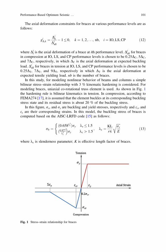
The axial deformation constraints for braces at various performance levels are asfollows:

giD;k ¼Dik

Diall

� 1� 0; k ¼ 1; 2; . . .; nb, i ¼ IO, LS, CP ð12Þ

where Dil is the axial deformation of a brace at ith performance level. Di

all for bracesin compression at IO, LS, and CP performance levels is chosen to be 0:25DC, 5DC,and 7DC, respectively, in which DC is the axial deformation at expected bucklingload. Di

all for braces in tension at IO, LS, and CP performance levels is chosen to be0:25DT, 7DT, and 9DT, respectively in which DT is the axial deformation atexpected tensile yielding load. nb is the number of braces.

In this study, for modeling nonlinear behavior of beams and columns a simplebilinear stress–strain relationship with 3 % kinematic hardening is considered. Formodeling braces, uniaxial co-rotational truss element is used. As shown in Fig. 1the hardening rule is bilinear kinematics in tension. In compression, according toFEMA274 [17], it is assumed that the element buckles at its corresponding bucklingstress state and its residual stress is about 20 % of the buckling stress.

In this figure, σcr and σy are buckling and yield stresses, respectively and εcr andεy are their corresponding strains. In this model, the buckling stress of braces iscomputed based on the AISC-LRFD code [15] as follows:

rb ¼ð0:658k2c Þry kc � 1:5

ð0:877k2c

�ry kc [ 1:5

(; kc ¼ KL

rp

ffiffiffiffiffiryE

rð13Þ

where λc is slenderness parameter; K is effective length factor of braces.

Fig. 1 Stress–strain relationship for braces

Performance-Based Optimum Seismic … 101

2.3 Optimization Problem Statement

The main aim of a sizing structural optimization problem is usually to minimize theweight of the structure subject to a number of design constraints. For a steelstructure with ne members that are collected in ng design groups, if the variablesassociated with each design group are selected from a given profile list of steelsections (such as W-shaped sections), a discrete optimization problem can be for-mulated as follows:

Find:X ¼ x1 x2 � � � xi � � � xng T ð14Þ

To minimize:wðXÞ ¼Xng

i¼1

qiAi

Xnmj¼1

Lj ð15Þ

Subject to: gkðXÞ� 0; k ¼ 1; 2; . . .; nc ð16Þ

where xi is an integer value expressing the sequence numbers of steel sectionsassigned to ith group; w represents the weight of the frame, ρi and Ai are weight ofunit volume and cross-sectional area of the ith group section, respectively; nm is thenumber of elements collected in the ith group; Lj is the length of the jth element in theith group; gk(X) is the kth behavioral constraint and nc is the number of constraints.

In this study, the constraints of performance-based optimum seismic design(PBOSD) problem is handled using the concept of exterior penalty functionsmethod (EPFM) [18]. The general approach of penalty function methods is tominimize the objective function as an unconstrained function but to provide somepenalty to limit constraint violations. In this case, the pseudo-unconstrainedobjective function is expressed as follows:

UðX; rpÞ ¼ wðXÞ 1þ PFr þ PFd þ PFh þ PFDð Þ ð17Þ

PFr ¼ rpXnel¼1

ðmaxf0; gr;lgÞ2 ð18Þ

PFd ¼ rpXIO;LS;CP

i

Xnsj¼1

ðmaxf0; gid;jgÞ2 ð19Þ

PFh ¼ rpXIO;LS;CP

i

Xnel¼1

ðmaxf0; gih;lgÞ2 ð20Þ

PFD ¼ rpXIO;LS;CP

i

Xnbk¼1

ðmaxf0; giD;kgÞ2 ð21Þ

102 S. Gholizadeh and H. Poorhoseini

where U, PFσ, PFd, PFθ, PFΔ, and rp are the pseudo objective function, penaltyfunction for serviceability check, penalty function for drift checks, penalty functionfor element plastic rotation checks, penalty function for braces’ axial deformationchecks, and positive penalty parameter, respectively.

3 Meta-Heuristic Algorithms

Meta-heuristics are popular due to their interesting characteristics for solving a widerange of continuous, discrete, and combinatorial complex optimization problems.Most of the meta-heuristics mimic natural phenomena to search the design space ofthe optimization problems. In recent years, it was found that meta-heuristic algo-rithms are computationally efficient even if greater number of optimization cycles isneeded to reach the optimum in comparison with gradient-based algorithms.Furthermore, meta-heuristic algorithms are more robust in finding the globaloptima, due to their random search, whereas mathematical programming algorithmsmay be trapped into local optima. In this work, PSO, FA, and BA meta-heuristicalgorithms are employed to tackle the stated optimization problem. The mainconcepts of the mentioned meta-heuristics are explained as follows:

3.1 Particle Swarm Optimization

PSO is a population-based meta-heuristic algorithm in which the population iscalled swarm and each individual in the swarm is called particle. Each particle ofthe swarm represents a potential solution of the optimization problem. Thismeta-heuristic algorithm first presented by Eberhart and Kennedy [19]. The parti-cles fly through the search space and their positions are updated based on the bestpositions of individual particles in each iteration. Using following equations theposition of the particles is updated:

Vkþ 1i ¼ xVk

i þ c1r1 Pkbest; i � Xk

i

� �þ c2r2 Gk

best � Xki

� � ð22Þ

Xkþ 1i ¼ Xk

i þVkþ 1i ð23Þ

where Xi and Vi represent the current position and the velocity of the ith particlerespectively; Pk

best; i is the best previous position of the ith particle (called pbest) and

Gkbest is the best global position among all the particle in the swarm (called gbest);

Positive constants c1 and c2 are the cognitive and social components, respectively;r1 and r2 are two uniform random sequences generated from range (0, 1) and ω isthe inertia weight used discount the previous velocity of the particle persevered.

Performance-Based Optimum Seismic … 103

Due to the importance of ω in achieving an efficient search behavior, theupdating criterion can be taken as follows:

x ¼ xmax � xmax � xmin

kmax� k ð24Þ

where xmax and xmin are the maximum and minimum values of x, respectively.Also, kmax, and k are the number of maximum iterations and the number of presentiteration, respectively.

In this work, the internal parameters of PSO are as follows: c1 = 2.0, c2 = 2.0,xmax ¼ 0:5 and xmin ¼ 0:0.

3.2 Firefly Algorithm

The FA, introduced by Yang [20], is a meta-heuristic optimization algorithminspired by the flashing behavior of fireflies. FA is a population-based algorithm,which may share many similarities with PSO. Fireflies communicate, search forpray, and find mates using bioluminescence with varied flashing patterns [21]. Inorder to develop the firefly algorithm, natural flashing characteristics of fireflieshave been idealized using the following three rules [20]:

a. All of the fireflies are unisex; therefore, one firefly will be attracted to otherfireflies regardless of their sex.

b. Attractiveness of each firefly is proportional to its brightness, thus for any twoflashing fireflies, the less bright firefly will move towards the brighter one. Theattractiveness is proportional to the brightness and they both decrease as theirdistance increases. If there is no brighter one than a particular firefly, it willmove randomly.

c. The brightness of a firefly is determined according to the nature of the objectivefunction.

The attractiveness of a firefly is determined by its brightness or light intensitywhich is obtained from the objective function of the optimization problem.However, the attractiveness β, which is related to the judgment of the beholder,varies with the distance between two fireflies. The attractiveness β can be defined by[22]

b ¼ b0e�c:r2 ð25Þ

where r is the distance of two fireflies, β0 is the attractiveness at r = 0, and γ is thelight absorption coefficient.

The distance between two fireflies i and j at Xi and Xj, respectively, is determinedusing the following equation:

104 S. Gholizadeh and H. Poorhoseini

rij ¼ Xi � Xj

¼ffiffiffiffiffiffiffiffiffiffiffiffiffiffiffiffiffiffiffiffiffiffiffiffiffiffiffiffiffiffiffiffiffiffiffiffiffiXd

k¼1ðxi;k � xj;kÞ2

rð26Þ

where xi,k is the kth parameter of the spatial coordinate xi of the ith firefly.In the firefly algorithm, the movement of a firefly i towards a more attractive

(brighter) firefly j is determined by the following equation [22]:

Xi ¼ Xi þ b0e�c:r2ijðXj � XiÞþ aðrand � 0:5Þ ð27Þ

where the second term is related to the attraction, while the third term is random-ization with α being the randomization parameter. Also rand is a random numbergenerator uniformly distributed in [0, 1].

In this work, the modified equation proposed in [23] for computing α isemployed as follows:

a ¼ amax � amax � amin

tmax� t ð28Þ

where αmax and αmin are the maximum and minimum values of α. Also, tmax andt are the numbers of maximum iterations and present iteration, respectively.

In this work, the internal parameters of FA are as follows: β0 = 1.0, γ = 1.0,αmax = 1.0, and αmin = 0.2.

3.3 Bat Algorithm

The BA meta-heuristic optimization algorithm is inspired from the echolocationbehavior of microbats. Echolocation is an advanced hearing based navigationsystem used by bats to detect objects in their surroundings by emitting a sound tothe environment. While they are hunting for preys or navigating, these animalsproduce a sound wave that travels across the canyon and eventually hits an object ora surface and returns to them as an echo. The sound waves travel at a constant speedin zones where atmospheric air pressure is identical. By following the time delay ofthe returning sound, these animals can determine the precise distance to circum-jacent objects. Further, the relative amplitudes of the sound waves received at eachindividual ear are used to identify shape and direction of the objects. The infor-mation collected this way of hearing is synthesized and processed in the brain todepict a mental image of their surroundings [24].

The echolocation characteristics of microbats in BA are idealized as the fol-lowing rules [25]:

Performance-Based Optimum Seismic … 105

1. All bats use echolocation to sense distance, and they also ‘‘know’’ the differencebetween food/prey and background barriers in some magical way;

2. Bats randomly fly with velocity Vi at position Xi with a fixed frequency fmin,varying wavelength λ and loudness A0 to search for prey. They can automati-cally adjust the wavelength (or frequency) of their emitted pulses and adjust therate of pulse emission r 2 [0, 1], depending on the proximity of their target;

3. Although the loudness can vary in many ways, it is assumed that the loudnessvaries from a large (positive) A0 to a minimum constant value Amin;

The position and velocity of each bat should be updated in the design spaceaccording to the following equations:

fi ¼ fmin þ fmax � fminð Þui ð29Þ

Vkþ 1i ¼ round Vk

i þ Xki � X�� �

fi� � ð30Þ

Xkþ 1i ¼ Xk

i þVkþ 1i ð31Þ

where fmin and fmax are the lower and upper bounds imposed for the frequency rangeof bats. ui 2 [0, 1] is a vector containing uniformly distribution random numbers;X� is the current global best solution;

A local search is implemented on a randomly selected bat from the currentpopulation using the following equation:

Xkþ 1 ¼ Xk þ roundðejAkþ 1Þ ð32Þ

where ej is a uniform random number in [−1, 1] selected for each design variable ofthe selected bat. Ak+1 is the average loudness of all the bats at the current iteration.Also, “round” is to discrete the continuous space into an integer/discrete one.

The loudness Ai and the rate ri of pulse emission have to be updated accordinglyas the iterations proceed. As the loudness usually decreases once a bat has found itsprey while the rate of pulse emission increases, the loudness can be chosen as anyvalue of convenience. In this work, A0 = 1 and Amin = 0 also, r0 = 0 and rmax = 1.

Akþ 1i ¼ aAk

i ð33Þ

rkþ 1i ¼ r0i 1� e�c:k

� � ð34Þ

where α and γ are constants.In this work, the internal parameters of BA are as follows: α = 0.9, γ = 0.01,

fmin = 0.0, and fmax = 1.0.

106 S. Gholizadeh and H. Poorhoseini

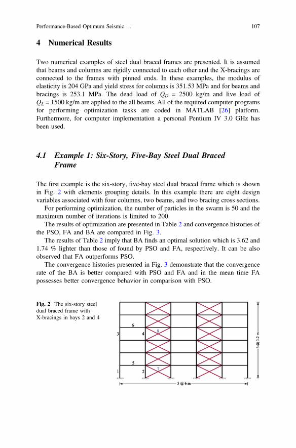
4 Numerical Results

Two numerical examples of steel dual braced frames are presented. It is assumedthat beams and columns are rigidly connected to each other and the X-bracings areconnected to the frames with pinned ends. In these examples, the modulus ofelasticity is 204 GPa and yield stress for columns is 351.53 MPa and for beams andbracings is 253.1 MPa. The dead load of QD = 2500 kg/m and live load ofQL = 1500 kg/m are applied to the all beams. All of the required computer programsfor performing optimization tasks are coded in MATLAB [26] platform.Furthermore, for computer implementation a personal Pentium IV 3.0 GHz hasbeen used.

4.1 Example 1: Six-Story, Five-Bay Steel Dual BracedFrame

The first example is the six-story, five-bay steel dual braced frame which is shownin Fig. 2 with elements grouping details. In this example there are eight designvariables associated with four columns, two beams, and two bracing cross sections.

For performing optimization, the number of particles in the swarm is 50 and themaximum number of iterations is limited to 200.

The results of optimization are presented in Table 2 and convergence histories ofthe PSO, FA and BA are compared in Fig. 3.

The results of Table 2 imply that BA finds an optimal solution which is 3.62 and1.74 % lighter than those of found by PSO and FA, respectively. It can be alsoobserved that FA outperforms PSO.

The convergence histories presented in Fig. 3 demonstrate that the convergencerate of the BA is better compared with PSO and FA and in the mean time FApossesses better convergence behavior in comparison with PSO.

Fig. 2 The six-story steeldual braced frame withX-bracings in bays 2 and 4

Performance-Based Optimum Seismic … 107

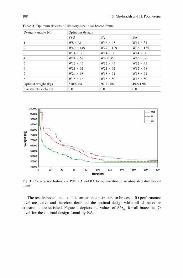
The results reveal that axial deformation constraints for braces at IO performancelevel are active and therefore dominate the optimal design while all of the otherconstraints are satisfied. Figure 4 depicts the values of Δ/Δall for all braces at IOlevel for the optimal design found by BA.

Table 2 Optimum designs of six-story steel dual braced frame

Design variable No. Optimum designs

PSO FA BA

1 W8 × 31 W16 × 45 W14 × 34

2 W40 × 149 W27 × 129 W36 × 135

3 W14 × 30 W14 × 30 W14 × 30

4 W24 × 68 W8 × 35 W16 × 36

5 W12 × 45 W12 × 45 W12 × 45

6 W21 × 62 W21 × 62 W12 × 58

7 W24 × 68 W18 × 71 W18 × 71

8 W18 × 46 W18 × 50 W18 × 50

Optimal weight (kg) 51092.64 50112.88 49241.98

Constraints violation 0.0 0.0 0.0

Fig. 3 Convergence histories of PSO, FA and BA for optimization of six-story steel dual bracedframe

108 S. Gholizadeh and H. Poorhoseini

4.2 Example 2: Twelve-Story, Five-Bay Steel Dual BracedFrame

Figure 5 shows the twelve-story steel frame with its elements grouping details.Design variable vector in this example includes sixteen components which are

divided to eight columns, four beams, and four bracing group cross sections. Thenumber of particles in the swarm and the maximum number of iterations are chosento be 50 and 400, respectively.

Table 3 reports the optimal designs found by PSO, FA, and BA and theirconvergence histories are depicted in Fig. 6.

Fig. 4 Δ/Δall values at IOlevel for the optimal six-storysteel dual braced frame foundby BA

Fig. 5 The twelve-story steeldual braced frame withX-bracings in bays 2 and 4

Performance-Based Optimum Seismic … 109

Table 3 Optimum designs of twelve-story steel dual braced frame

Design variable No. Optimum designs

PSO FA BA

1 W30 × 90 W30X90 W30X90

2 W36 × 160 W40 × 167 W33 × 141

3 W30 × 90 W10 × 68 W27 × 84

4 W30 × 108 W30 × 108 W27 × 84

5 W21 × 68 W12 × 45 W21 × 48

6 W24 × 76 W27 × 94 W24 × 68

7 W16 × 31 W16 × 31 W16 × 40

8 W24 × 68 W30 × 90 W21 × 48

9 W18 × 97 W8 × 67 W18 × 55

10 W8 × 67 W12 × 45 W16 × 89

11 W10 × 39 W18 × 50 W18 × 50

12 W16 × 40 W16 × 40 W18 × 50

13 W10 × 60 W10 × 60 W21 × 68

14 W16 × 50 W21 × 57 W21 × 57

15 W18 × 46 W18 × 46 W18 × 46

16 W6 × 25 W10 × 19 W6 × 25

Optimal weight (kg) 84018.92 82544.74 81274.68

Constraints violation 0.0 0.0 0.0

Fig. 6 Convergence histories of PSO, FA, and BA for optimization of twelve-story steel dualbraced frame

110 S. Gholizadeh and H. Poorhoseini

The reported results in Table 3 exhibit that the optimal solution found by BA is,respectively, 3.27 and 1.56 % lighter than the solutions found by PSO and FA. Inaddition, FA converges to an optimal solution which is 1.75 % lighter than that ofPSO.

Comparison of the convergence histories of Fig. 6 signifies that the BA pos-sesses better convergence behavior with respect to PSO and FA. Furthermore, FA isbetter than PSO in terms of convergence rate.

In this example, the active constraints which dominate the design are the axialdeformation of braces and the lateral drift constraints at IO performance level. Forthe BA optimal design, the values of Δ/Δall for all braces and the lateral drift profileat IO level are given in Figs. 7 and 8, respectively.

Fig. 7 Δ/Δall values at IO level for The optimal twelve-story steel dual braced frame found by BA

Performance-Based Optimum Seismic … 111

5 Conclusions

This chapter presents a comparative study on the computational performance ofpopular PSO, FA, and BA meta-heuristic algorithms for tackling the problem ofperformance-based optimum seismic design of steel dual braced frames. During theoptimization process two types of constraints have to be checked. To ensure ser-viceability of the design, each structural element is checked to satisfy theAISD-LRFD constraints for the non-seismic load combinations. While the secondtype includes the check of inter-story drifts, plastic rotation of beams and columnsand the axial deformation for braces at IO, LS and CP performance levels accordingto the FEMA-356 provisions for the seismic load combinations. To achieve this, theseismic responses of structures are evaluated by conducting nonlinear pushoveranalysis.

Two numerical examples including six-story and twelve-story steel dual bracedframes are presented. The optimization task is achieved using PSO, FA, and BAmeta-heuristics and the results are compared. The numerical results demonstratethat in the first example, BA finds a solution which is 3.62 and 1.74 % lighter thanthose of the PSO and FA, respectively. The results imply that the solution found byFA is slightly better than the PSO. It is observed that axial deformation constraintsfor braces at IO performance level dominate the optimal design. In the secondexample, the optimal weight of BA is 3.27 and 1.56 % lighter than those of the PSOand FA, respectively, and the solution of FA is slightly lighter than that of PSO.

Fig. 8 Drift profile at IOlevel for the optimaltwelve-story steel dual bracedframe found by BA

112 S. Gholizadeh and H. Poorhoseini

Moreover, the axial deformation of braces and the lateral drift constraints at IO leveldominate the optimal designs. In both numerical examples the convergence rate ofBA is better than those of the PSO and FA.

It can be finally concluded that for solving the complex and highly nonlinearoptimization problem of performance-based seismic design of steel dual bracedframes, the BA provides results which are better than those of the PSO and FAmeta-heuristics in terms of optimal weight and convergence rate. Therefore, BA canbe effectively employed to design cost-efficient steel structures with desirableseismic performance.

References

1. Gholizadeh, S.: Performance-based optimum seismic design of steel structures by a modifiedfirefly algorithm and a new neural network. Adv. Eng. Softw. 81, 50–65 (2015)

2. Gholizadeh, S., Moghadas, R.K.: Performance-based optimum design of steel frames by animproved quantum particle swarm optimization. Adv. Struct. Eng. 17, 143–156 (2014)

3. Kaveh, A., Laknejadi, K., Alinejad, B.: Performance-based multi-objective optimization oflarge steel structures. Acta. Mech. 223, 355–369 (2012)

4. Fragiadakis, M., Lagaros, N.D.: An overview to structural seismic design optimisationframeworks. Comput. Struct. 89, 1155–1165 (2011)

5. Liu, M., Burns, S.A., Wen, Y.K.: Multiobjective optimization for performance-based seismicdesign of steel moment frame structures. Earthq. Eng. Struct. Dyn. 34, 289–306 (2005)

6. Fragiadakis, M., Lagaros, N.D., Papadrakakis, M.: Performance-based multiobjectiveoptimum design of steel structures considering life-cycle cost. Struct. Multidisc Optim. 32,1–11 (2006)

7. Kaveh, A., Farahmand Azar, B., Hadidi, A., Rezazadeh Sorochi, F., Talatahari, S.:Performance-based seismic design of steel frames using ant colony optimization. J. Constr.Steel Res. 66, 566–574 (2010)

8. Yang, X.S.: A new metaheuristic bat-inspired algorithm. In: Gonzalez, J.R. et al. (eds.) NatureInspired Cooperative Strategies for Optimization (NISCO 2010). Studies in ComputationalIntelligence, vol 284, pp. 65–74. Springer: Berlin (2010)

9. Gholizadeh, S., Shahrezaei, A.M.: Optimal placement of steel plate shear walls for steel framesby bat algorithm. Struct. Des. Tall Spec. Buil. 24, 1–18 (2015)

10. Hasancebi, O., Carbas, S.: Bat inspired algorithm for discrete size optimization of steel frames.Adv. Eng. Softw. 67, 173–185 (2014)

11. Hasancebi, O., Teke, T., Pekcan, O.: A bat-inspired algorithm for structural optimization.Comput. Struct. 128, 77–90 (2013)

12. FEMA-273 (1997) NEHRP guideline for the seismic rehabilitation of buildings. FederalEmergency Management Agency, Washington

13. FEMA-356 (2000) Prestandard and commentary for the seismic rehabilitation of buildings.Federal Emergency Management Agency, Washington

14. McKenna F, Fenves GL (2001) The OpenSees Command Language Manual (1.2. edn). PEER15. Manual of steel construction: Load and Resistance Factor Design. American Institute of Steel

Construction, Chicago, IL (2001)16. Sullivan, T.J., Calvi, G.M., Priestley, M.J.N., Kowalsky, M.J.: The limitations and

performances of different displacement based design methods. J. Earthq. Eng. 7, 201–241(2003)

17. Federal Emergency Management Agency: NEHRP guidelines for the seismic rehabilitation ofbuildings, Rep. FEMA 273 (Guidelines) and 274 (Commentary), Washington (1997)

Performance-Based Optimum Seismic … 113

18. Vanderplaats, G.N.: Numerical Optimization Techniques for Engineering Design: WithApplication, 2nd edn. McGraw-Hill, New York (1984)

19. Eberhart, R.C., Kennedy, J.: A new optimizer using particle swarm theory. In: Proceedings ofthe Sixth International Symposium on Micro Machine and Human Science, pp. 39–43. IEEEPress, Nagoya (1995)

20. Yang, X.S.: Firefly algorithms for multimodal optimisation. In: Watanabe, O., Zeugmann, T.(eds.) Procedings of the 5th Symposium on Stochastic Algorithms, Foundations andApplications. Lecture Notes in Computer Science, vol. 5792, pp 169–178 (2009)

21. Gandomi, A.H., Yang, X.S., Alavi, A.H.: Mixed variable structural optimization using fireflyalgorithm. Comput. Struct. 89, 2325–2336 (2011)

22. Yang, X.S.: Firefly algorithm, stochastic test functions and design optimization. Int.J. Bio-Inspired Comput. 2, 78–84 (2010)

23. Gholizadeh, S., Barati, H.: A comparative study of three metaheuristics for optimum design oftrusses. Int. J. Optim. Civil Eng. 2, 423–441 (2012)

24. Carbas, S, Hasancebi, O.: Optimum design of steel space frames via bat inspired algorithm. In:10th World Congress on Structural and Multidisciplinary Optimization, Florida, USA (2013)

25. Gandomi, A.H., Yang, X.S., Alavi, A.H., Talatahari, S.: Bat algorithm for constrainedoptimization tasks. Neural. Comput. Appl. 22, 1239–1255 (2013)

26. MATLAB: The Language of Technical Computing. Math Works Inc (2011)

114 S. Gholizadeh and H. Poorhoseini

Genetic Algorithms for Optimization of 3DTruss Structures

Vedat Toğan and Ayşe Turhan Daloğlu

Abstract Various optimization techniques have been applied to find the optimumsolutions of structural design problems in the last 50 or 60 years. Simple structuraloptimization problems with continuous design variables have been solved initiallyusing mathematically diverse techniques. New approaches called meta-heuristictechniques have been emerging along with the progress of traditional methods. Thischapter first introduces the mathematical formulations of optimization problems andthen gives a summary and development process of the preliminary techniques suchas genetic algorithm (GA) in obtaining the optimum solutions. The mathematicalformulations of the structural optimization problems are associated with the designvariables, loads, structural responses, and constraints. Strategies are proposed toimprove the performance of the technique to reduce the number of search and thesize of the problem. Finally, some examples related to 3D truss structures arepresented.

1 Introduction

Optimization of the structures is one of the main research areas in civil andstructural engineering. As a branch of applied and computational mathematics,optimization usually tries to find the best-fitted solution of the problem within adomain that contains acceptable values of design variables subject to some designrestrictions or constraints. The optimum solution of the problem may be achievedby minimizing or maximizing a real objective function satisfying predefinedrestrictions at the same time. Such a solution is supposed to be the best one among alarge feasible solution space that can satisfy all the constraints of the optimizationproblem. The function to be minimized or maximized is referred to as objective

V. Toğan � A.T. Daloğlu (&)Department of Civil Engineering, Karadeniz Technical University,61080 Trabzon, Turkeye-mail: aysed@ktu.edu.tr

© Springer International Publishing Switzerland 2016X.-S. Yang et al. (eds.), Metaheuristics and Optimization in Civil Engineering,Modeling and Optimization in Science and Technologies 7,DOI 10.1007/978-3-319-26245-1_6

115

function, while the functions to represent restrictions are called as constraints. Thedesign parameters of an optimization problem are called design variables. While thegeometric properties of members can be considered as design variables in structuralweight optimization, coordinates of nodal points can be treated as design variablesfor shape or topology design of structures. So the objective function, constraints,and variables can vary widely according to the type of the problem. For the min-imum weight design of 3D truss structures, the objective function represents theweight of the truss, variables can be the areas of cross sections of the structuralmembers, and the constraints may be the maximum allowable stresses and dis-placements of nodal joints.

2 Mathematical Formulations of Optimization Problems

An optimization problem subject to some constraints can be formulated as thefollowing mathematical form:

minx2 S

f ðxÞS ¼ xjhjðxÞ ¼ 0; j ¼ 1; . . .; p; gkðxÞ� 0; k ¼ 1; . . .;m

� � ð1Þ

where f(x), hj(x), and gk(x) are a C1 function of x 2 IRn. In addition, p and m arethe total numbers of hj(x) and gk(x), respectively. S represents the feasible set for theoptimization problem, S � IRn.

However, in the engineering field, an optimization problem can also be generallydefined as follows:

find x ¼ x1; x2; . . .; xnf gmin: WðxÞs:t: gkðxÞ� 0; k ¼ 1 tom

xil � xi � xiu; i ¼ 1 to n

ð2Þ

In Eqs. (1) and (2), x is an n-dimensional vector representing the design variables ofthe optimization problem. Depending on the optimization type, the cross-sectionalareas of the members, the nodal coordinates of the member connections, and themembers itself are treated as the design variables. f(x) and W(x) are called objectivefunctions or cost functions, which usually correspond to a real number to be used toevaluate how good a solution is. Since weight is usually adopted as the objectivefunction of the optimization problem in structural engineering, W(x) corresponds tothe weight of the related structure. hj(x) and gk(x) are the equality and inequalityconstraints functions, respectively. In contrast, hj(x) in the engineering fields, thetype of inequality constraint functions, gk(x), are often encountered. And it generallyrequires a structural analysis to obtain the structural response such as displacements,

116 V. Toğan and A.T. Daloğlu

forces, etc. Here, xil and xiu show the lower and upper boundaries of xi. Strictlyspeaking, xi might be continuous, discrete, and real but since it is preferred inpractice to select the cross-sectional areas of members from the predefined list, xi istaken as the discrete in structural engineering applications.

3 Genetic Algorithms

To find the value of x obeying the hj(x) and gk(x) and minimizing W(x) requires anoptimization method to be employed. Optimization methods, generally speaking,are classified as the gradient-based and gradient-free techniques. Of course, variouscategorizations can be encountered for the optimization methods available in theliterature [1–3]. In fact, although they are referred with various classifications andnames, there is not much difference in the main properties of the methods. Forexample, one of the most commonly used classifications is deterministic andstochastic. While the former uses derivatives of the objective function and con-straints in the search of the optimum solution, the latter works with probabilistictransition rules instead of the gradient information of the objective function andconstraints [4–12]. As seen from the example, deterministic and stochastic tech-niques are easily put into the classification of the gradient-based and thegradient-free optimization methods, respectively.

Genetic algorithm (GA) is probably one of the first optimization methods, whichsimulates the natural phenomena into a numerical algorithm. It mimics the proce-dure known as survival of the fittest. GA was firstly proposed by Holland [13].Since new some valuable improvements in the GA such as adaptive operators,distinct coding schemes for the design variables, immigration, elitism, breeding,hybridization, etc., have been presented by the researcher [19–30].

After the study of Rajeev and Krishnamoorthy [14] which was awell-documented study for the application of the GA in the structural optimizationproblems, GA has gained more popularity in this area than that proposed for thefirst time. By studying Rajeev and Krishnamoorthy [14], it is realized at first glancethat GA is very primitive compared with the level recently reached. For instance,the design variables were coded with binary scheme in the GA process proposed byRajeev and Krishnamoorthy [14], while at the moment the design variables aretreated as discrete and even that mixed [15–18]. Figure 1 demonstrates the binaryscheme for the design variables of the structural optimization problems. Herein, it isassumed that the corresponding optimization problem has three design variables

1011 0100 0110x=[ x1 x2 x3 ]

Fig. 1 Coding in binary system for design variables

Genetic Algorithms for Optimization of 3D Truss Structures 117

which are the cross-section areas of the grouped members. And they are selectedfrom 16 different sections available in practice.

When this scheme is chosen to find the value of the design variables in decimalsystem, a transformation is needed. Through this transformation, the sequencenumbers of the sections related to the design variables are determined from apredefined list sections. The steps of the transformation and mapping can besummarized as the main steps shown in Fig. 2. After mapping with the predefinedlist, the cross-section area for the related design variable is directly used in thecorresponding process, i.e., in calculating the structural responses via a structuralanalyzer.

Then the structure should be analyzed to determine its responses and then therequirements of the optimization problems defined by the constraints functions areevaluated. The next step is to calculate the value of W(x). As mentioned before, itshows the goodness of the solution that consists of coupling the design variables(see Fig. 1)—the string is called as a solution. However, since the GA is anunconstrained optimization method like other gradient-free optimization tech-niques, W(x) also includes the value of a function known as the penalty functionwhich reflects the violation level of the constraints in normalized form for thesolution. Equation (3) shows the objective function, incorporating the constraintsviolation as expressed in Rajeev and Krishnamoorthy [14].

20x1+21x0+22x1+23x1 20x0+21x1+22x0+23x0 20x0+21x1+22x1+23x0

1+0+4+8=13 0+2+0+0=2 0+2+4+0=6

20x1+21x0+22x1+23x1 20x0+21x1+22x0+23x0 20x0+21x1+22x1+23x0

1+0+4+8= 0+2+0+0= 0+2+4+0=

1011 0100 0110Transformation from binary to decimal system

Mapping with pre-Section no

Area(mm2) available in practice

1 0.452 0.48

6 0.957 1.02

13 1.35

defined list

Fig. 2 Decoding and mapping steps for the design variables represented in the binary system

118 V. Toğan and A.T. Daloğlu

WðxÞ ¼ W 0ðxÞ 1þKCð Þ

where C ¼Xmk¼1

ckð3Þ

where K is a parameter that is taken as 10, C is the violation coefficient computed inthe following manner: if gk(x > 0, then ck = gk(x); or if gk(x ≤ 0), then ck = 0.Finally, W′(x) represents the weight of the structure. Note that gk(.) is in the nor-malized form expressed as σ/σa −1 ≤ 0 for stress and d/da−1 ≤ 0 for displacement.σa and da in these expressions show the allowable values for stress and displace-ment for the problem considered.

3.1 Genetic Operators

The search procedures of GA were based on the mechanics of natural genetics andnatural selection. With the help of the genetic operators adapted from nature, theconcept of the survival of the fittest is simulated to form a robust search mechanism.Following the steps summarized above, the GA search procedure proposed byRajeev and Krishnamoorthy [14] applies two genetic operators successively.

The first one is the reproduction operator which reflects the concept of thesurvival of the fittest in nature. It proceeds according to the individual fitnesscalculated as follows:

Fi ¼ Wmax þWminð Þ �WiðxÞ ð4Þ

where Fi is the fitness of the ith individual in the population, Wmax and Wmin are themaximum and minimum values of W(x) computed using Eq. (3). Thus, the indi-viduals with higher fitness values have a higher probability to survive, whereas theless fit ones get fewer chances of survival. And the worst fit individuals will beremoved from the population.

Then, to exchange the solution segments between the individuals in the popu-lation, crossover operator is implemented. Double point crossover is applied to thepairs selected randomly as an example. Figure 3 demonstrates the application of thetwo genetic operators explained in Rajeev and Krishnamoorthy [14].

The genetic algorithm continues the process by following the above steps out-lined in detail so as to modify the new population. To terminate the GA process, acriterion based on the similarity of the individuals in the population was imposed byRajeev and Krishnamoorthy [14]. In addition, although mutation operator was notimplemented in [14], the GA search process employed it to preserve the diversityamong the population. Figure 4 illustrates the basic concept behind the mutationoperator. It proceeds in three steps. First, an individual within the population israndomly selected. Then, a binary position to be changed is determined randomly.

Genetic Algorithms for Optimization of 3D Truss Structures 119

Fitness(Fi/Fave)

Tra

nsfo

rmat

ion

from

bi-

nary

to d

ecim

al s

yste

m

Map

ping

with

the

pred

e-fi

ned

sect

ion

lists

Cal

cula

te s

truc

tura

l re-

spon

se

App

ly E

q.(3

)th

en E

q.(4

) 0.83 preserve

1.48 preserve

0.26 eliminate

Pairs Site 1 Site 2 New population4 5 10 1011 0011 1010

1 5 10 1100 0100 01118 2 6

5 2 6

individualIn

divi

dual

num

ber

Design variablesx1 x2 x3

1011 0100 0110

1100 0011 1011

0011 1101 0001

1011 0100 0110

1100 0011 1011

1100 0011 1011

(a)

(b)

Fig. 3 Two genetic operators given in Rajeev and Krishnamoorthy [14]. a Reproduction operator.b Crossover operator

Available popula-tion

Individual number to be exposed to

mutation

Position number New individual

1011 0011 1010

8 7 1010 0011 00111100 0100 0111

1010 000 00111

Fig. 4 Mutation operator

120 V. Toğan and A.T. Daloğlu

After that, the corresponding position value is switched to 1 if it is equal to 0 or to 0if it is equal to 1.

All search procedures based on GA were called simple genetic algorithms inRajeev and Krishnamoorthy [14] and since then, numerous modifications have beenproposed by researchers in order to improve the search and/or computationalperformances of the GA in this area. For example, the coding scheme [19–21],the penalization [22–27], and new operators [28–30] are some of them. Otherimprovements based on adaptive concept have attracted more attention. The fol-lowing section will review this concept.

4 Strategies Based on the Adaptive Concept

Some improvement or renewal in the GA operators or the GA algorithms have beenmade by researchers to increase the probability of finding the global solution and toenhance the performance of GA. Other improvements of GA are to relieve the userfrom the burden of determining sensitive parameter(s) existed in GA. The vastmajorities of these efforts have been focused on the adaptive approaches in GA forboth the penalty function, and the mutation and crossover. The key idea behind theadaptive approaches is to adjust itself automatically during the optimization pro-cedure using genetic algorithms.

4.1 Adaptive Penalty Scheme

Although it is not a genetic operation, the penalty function is important in GA todemonstrate the extent of the violation of the constraints quantitatively. Penaltytechniques can be classified as multiplicative or additive. A positive penalty factoris introduced in the multiplicative case to amplify the value of the fitness function ofan infeasible individual in a minimization problem. This type of penalty hasreceived less attention in the evolutionary computation community, compared withthe additive type. A penalty functional is added to the objective function in theadditive case to define the fitness value of an infeasible element [24].

An adaptive penalty scheme to be able to adjust itself automatically during theGA process is proposed by Toğan and Daloğlu [31] as follows:

fpenalty ¼ Cmax þCðrÞð Þ= Cmax þCaveð Þ CðrÞ�Cave

fpenalty ¼ Cave þCðrÞð Þ= Cave � Cminð Þ CðrÞ\Cave

fpenalty ¼ 0 CðrÞ ¼ 0 r ¼ 1; . . .; nps

ð5Þ

where fpenalty is the penalty function, C(r) is the violation value of normalizedconstraints of the rth individual in the generation, and nps represents the population

Genetic Algorithms for Optimization of 3D Truss Structures 121

size. In addition, Cmax, Cmin, and Cave are, respectively, the maximum, minimumand average violation values of generation. According to this formulation, Eq. (3)becomes

WðxÞ ¼ W 0ðxÞ 1þ fpenalty� �

: ð6Þ

The penalty function is, therefore, kept free from any predefined or user-definedconstants. Also the magnitudes of the violations are not characterized by a staticrate for both near feasible and infeasible solutions during the design process. Withthe expressions in Eq. (5), the infeasible solutions will not be penalized with thesame rate of penalty. The magnitude of the penalty tends to get heavier instead, asthe level of the violation of the infeasible solution tends to get bigger. Moreover,the magnitude of penalty increases as the violation value gets closer to Cmax. On theother hand, it decreases as the violation value gets closer to Cmin. Thus, someinfeasible individuals that are close to the feasible region in the search space willnot disappear through the penalty scheme and they will find a chance to survive.This may sustain the capacity of finding the global solution for design problemusing GA.

4.2 Adaptive Crossover and Mutation Schemes

Genetic operators are applied to mimic the natural evolution. Among these oper-ators, crossover provides the genetic information exchange between the couplesrandomly, and mutation enables the development of new genetic material, and bothplay an effective role to reach the optimum or to get close to the optimum solution.It is arbitrary and up to the user to incorporate the rates of these operators inoptimization process. The choices of mutation, pm, and crossover, pc, rates as wellas generating positions to be shifted by mutation and mapping the individuals forcrossover are also arbitrary.

Many refinements using adaptive controls provide significant improvements inperformance for some situations [32]. Keeping all of these in mind, it can beconcluded that the randomness on mapping for crossover, and specifying the geneposition(s) for mutation may be removed. Mutation and crossover should beadapted for both the individual and the generation because it is possible to lose thebest-fitted individual with this random process in mutation. Therefore, in contrast totraditional crossover and mutation operator based on randomization mechanisms,i.e., generating the pairs, and determining position of bit shifted by mutation of thesolution, the mutation and the crossover operators can be adaptive and adjustthemselves from generation to generation since the population is renewed fromiteration to iteration. Adaptive means adjusting itself automatically depending onthe fitness value of the individual and the other individuals in the generation.

122 V. Toğan and A.T. Daloğlu

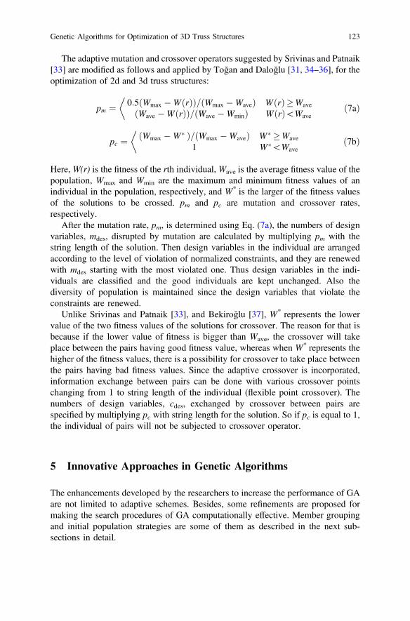
The adaptive mutation and crossover operators suggested by Srivinas and Patnaik[33] are modified as follows and applied by Toğan and Daloğlu [31, 34–36], for theoptimization of 2d and 3d truss structures:

pm ¼ 0:5 Wmax �WðrÞð Þ= Wmax �Waveð Þ WðrÞ�Wave

Wave �WðrÞð Þ= Wave �Wminð Þ WðrÞ\Wave

�ð7aÞ

pc ¼ Wmax �W�ð Þ= Wmax �Waveð Þ W� �Wave

1 W�\Wave

�ð7bÞ

Here, W(r) is the fitness of the rth individual, Wave is the average fitness value of thepopulation, Wmax and Wmin are the maximum and minimum fitness values of anindividual in the population, respectively, and W* is the larger of the fitness valuesof the solutions to be crossed. pm and pc are mutation and crossover rates,respectively.

After the mutation rate, pm, is determined using Eq. (7a), the numbers of designvariables, mdes, disrupted by mutation are calculated by multiplying pm with thestring length of the solution. Then design variables in the individual are arrangedaccording to the level of violation of normalized constraints, and they are renewedwith mdes starting with the most violated one. Thus design variables in the indi-viduals are classified and the good individuals are kept unchanged. Also thediversity of population is maintained since the design variables that violate theconstraints are renewed.

Unlike Srivinas and Patnaik [33], and Bekiroğlu [37], W* represents the lowervalue of the two fitness values of the solutions for crossover. The reason for that isbecause if the lower value of fitness is bigger than Wave, the crossover will takeplace between the pairs having good fitness value, whereas when W* represents thehigher of the fitness values, there is a possibility for crossover to take place betweenthe pairs having bad fitness values. Since the adaptive crossover is incorporated,information exchange between pairs can be done with various crossover pointschanging from 1 to string length of the individual (flexible point crossover). Thenumbers of design variables, cdes, exchanged by crossover between pairs arespecified by multiplying pc with string length for the solution. So if pc is equal to 1,the individual of pairs will not be subjected to crossover operator.

5 Innovative Approaches in Genetic Algorithms

The enhancements developed by the researchers to increase the performance of GAare not limited to adaptive schemes. Besides, some refinements are proposed formaking the search procedures of GA computationally effective. Member groupingand initial population strategies are some of them as described in the next sub-sections in detail.

Genetic Algorithms for Optimization of 3D Truss Structures 123

5.1 Initial Population Strategy

To start the evolution process in GA, the initial population within the solution spaceis generated. All individuals constituting the initial population are selected from thesolution space of the problem notwithstanding any condition. In other words, thisstep is random. However, even though the process of creating initial populationseems ordinary, it critically affects the convergence, the performance and the abilityof the GA. This case becomes more crucial for very complicated and large solutionspace which is mostly encountered in the practical application of GA in the area ofstructural engineering.

The idea starting the search of the solution space without a randomly generatedset is the key rationale of creating the initial population automatically. So, adoptingthe list number of the maximum area of cross sections as the starting point for thedesign variables leads to more efficiency than randomly generated. And it is storedas the initial point for each group of tension members to create the initial popu-lation. For the groups of the compression members, two or three surplus of the listnumber of the member that has he maximum area of cross section in the group istaken from the list of sections. The value of cross-sectional area and radius ofgyration of that section must be bigger than the values found previously. And thecorresponding section list number gives the initial points for each group of com-pression members and is stored to create the initial population (see Toğan andDaloğlu [31, 34] for more details).

5.2 Member Grouping Strategies

In the structural optimization terminologies, the design variables refer to the vari-ables affecting the value of the objective function, and they generally represent theareas of the cross section of the structural members. Since the GA completelyindependent from the characteristic of the problem, the design variables of theoptimization problems should be coded in some encoding schemes such as binary,decimal, real, and so on. GA evolves those solutions by creating in terms of designvariables and randomly selecting into the potential solutions space of the problem.A set of possible feasible or unfeasible solutions construct the population or gen-eration. Each solution in the populations is known as the individual.

For a given problem, all of the cross-sectional areas of the structural memberscan be taken as design variables. In this case, however, the computation time getsvery high and the results obtained from optimization process will probably be thelocal optima due to the expanded design space. Therefore in the GA applications,member grouping is generally applied for the members of the structural system inorder to reduce the size of the problem. On the other hand, the member groupingadopted a priori might not lead to an accurate grouping and if the number ofmembers of the structural systems becomes very large; i.e., for 3D roof trusses,

124 V. Toğan and A.T. Daloğlu

transmission towers, this leads to very large string lengths, which delays conver-gence and precludes useful exchange of information [38].

Two new member grouping strategies are proposed by Toğan and Daloğlu [31,34] to reduce the size of the search space of the design problem as much aspossible, to increase the probability of catching the global optimum solution andenhance the performance of the GA. The key idea behind the member groupingstrategies is to make a convenient member grouping that will end up with as fewnumbers of cross sections as possible in the final set, and reduce the size of thedesign space of the problem as much as possible. The efforts are also made torelieve the user from the burden of determining the member groups.

5.2.1 First Member Grouping Strategy

The first strategy (strategy 1) is based on the one proposed by previous researchers[31, 38, 39]. To implement this strategy, the same cross-section areas are assignedfor all the structural members first as stated in [31, 38, 39]. Then the analysis of thestructure is performed using these initial areas for each load cases. Following thestatic analysis, the entire range of internal forces is divided into several ranges bothfor tension and compression members. And members are grouped according to theinternal forces in the members.

An additional group is added in Toğan and Daloğlu [34] to the system for zeroforce members or members with very low internal forces. Hence, all the members ofthe truss structure are grouped conveniently and accurately. Moreover, a complexsolution space may be avoided under some conditions.

5.2.2 Second Member Grouping Strategy

For strategy 2, while the magnitude of the axial force is considered as the factor forgrouping the tension members [31, 38, 39], slenderness ratio is considered as themain factor for the compression members to set the groups. Therefore, due to theimportance of slenderness ratio, it may be more convenient to group the com-pression members according to their slenderness ratio in terms of radius of gyrationof the cross section and the effective length of the member instead of grouping themdepending on the magnitude of the axial force. This is the key idea behind strategy2. Hence, as the tension members of the truss structure are grouped depending onthe axial forces, the compression members are grouped according to their slen-derness ratio. An extra member group for the zero force members or members withvery low internal forces is also arranged (Toğan and Daloğlu [31, 34]).

Genetic Algorithms for Optimization of 3D Truss Structures 125

6 Examples

In this section, in the light of the information given in the previous sections, twotypes of design examples are presented. In the first one, a 160-bar space truss isconsidered as an example to demonstrate the effectiveness and robustness of pro-posed adaptive approaches for GA and member grouping strategy over simple GA.Later, an investigation is performed to demonstrate the efficiency, accuracy, andreliability of the proposed initial population strategies by solving numericalexamples taken from previous studies in the literature for comparison.

The population size is taken as 40 for all the examples and real-value coding isemployed in the genetic algorithm.

At the beginning of the genetic process 40 % of the initial population is createdby using the proposed initial population strategy automatically. Therefore thediversity of the population is preserved and the algorithm may be less likely to getstuck at local minima and may also avoid some early convergence. It is possible tocreate all the individuals of the initial population automatically. However, in thiscase, the initial population consists of the same individual only and the searchperformed in the solution space start in a certain region. On the other hand, as theadaptive schemes applied for both penalty functions and mutation and crossoveroperators are able to adjust itself automatically during the genetic process [31], theycompletely disrupt the initial population. So, creating all the individuals in theinitial population automatically is not meaningful.

6.1 Example 1: 160-Bar Truss Tower

The 160-bar truss tower shown in Fig. 5 was optimized by Rajaev andKrishnamoorthy [14] and Galante [40] in advance. 32 cross-section types were usedto optimize the tower and taken from the AISC Manual [41]. The members areclassified into 16 groups. Details of the member groups were presented in Galante[40]. Rajaev and Krishnamoorthy [14] used in GA with one criterion (minimumweight) and without taking the buckling effect into account. As Galante [40] stated,it can be observed that the buckling effect plays an important role in truss opti-mization. So if it is not taken into account the truss obtained will not be suitable asload carrying structural system. Galante [40] optimized the transmission tower withthe aim of the minimum weight and minimum number of cross-section types of barstaken from the market and also taking buckling and the slenderness limits rec-ommended by AISC [41] into account.

The tower is optimized for the objective indicated by Galante [40] with theproposed algorithm. All parameters needed to start the optimization process aretaken from the reference studies. The structure is optimized with the implementedimprovements in GA and two member grouping strategies for the aim of that thefinal design forms three groups at one for tension and two for compression

126 V. Toğan and A.T. Daloğlu

members. An extra member group for zero force members is not formed. This isbecause of the fact that Galante [40] reported that 51 bars have a higher com-pression stress than the limit recommended by AISC [41] to prevent buckling and68 have higher slenderness ratio than the AISC advice. It is also observed from theoptimization process of the tower that the arrangement of an extra member groupfor zero force members does not make any difference in the weight of the towerdrastically and the two member grouping strategies give the same result. Therefore,the tower is optimized with three, four, and five member groups.

The final design obtained by the proposed strategies and the ones reported byGalante [40] are presented in Table 1. Galante [40] used both GA and the simplerebirth process in GA for the optimization of this example and mentioned that theGA with the rebirth process achieves a better truss. However, the optimum designsobtained with the proposed improvements in the algorithm ended up with a lightertruss than the design by Galante [40]. A question may arise: as the values of designvariables presented in Table 1 for the three groups are the same, why are theoptimum weight of truss different? The answer is hidden in Fig. 6a. It is shown inFig. 6a that some members that belong to the first group skipped to the secondgroup and a better solution from the previous one is reached. However, the mostinteresting result is obtained when the four member groups are adopted at two fortension and two for compression member for this example. Although this optimumdesign has more groups than the result obtained by Galante [40] and previouslyperformed optimization cases, in this study, it seems still reasonable to achieve thatthe number of sections in the final set must be as few as possible to make fabri-cation and workmanship easier [31, 39, 40]. The reduction in the total weight of the

Fig. 5 160-bar trussed steel transmission tower

Genetic Algorithms for Optimization of 3D Truss Structures 127

Table 1 Comparison of results for 160-bar transmission tower

Designvariables(mm2)

Galante [40]at 3 groupsby the GA

Galante [40] at 3groups by the GAwith rebirth

This study

At 3groups

At 3groups

At 4groups

At 5groups

A1 2812 767.74 767.74 767.74 767.74

A2 3064 581.93 581.93 339.99 339.99

A3 7096 1251.61 1251.61 581.93 581.93

A4 1251.61 1251.61

A5 150.96

Weight(kN)

15.33 14.61 14.269 12.651 10.544 10.449

Fig. 6 aMember groups for 160-bar tower, b Variation of weight for the three cases with numberof generations

128 V. Toğan and A.T. Daloğlu

tower is about 28 % compared to the designs summarized in Table 1. As mentionedabove, when the number of groups is taken as five, the optimized weight is slightlychanged. In other words, arranging an extra group for the zero force members didnot affect the weight of the tower drastically. Hence, the design at four groups ismore meaningful than the design at five groups for the design objective. Figure 6bshows the genetic histories of the value of the objective function taken as the weightof tower for three optimization cases.

6.2 Example 2: 640-Bar Space Deck Truss

A trussed space deck shown in Fig. 7 has 179 joints and 640 members. The trusswas first studied by Jenkins [32] in order to assess the decimal GA on a moresubstantial structural problem. Jenkins [32] found the optimum height of truss inaddition to optimum volume. The truss members were subjected to compressivestress limitation given in BS 5950 and tensile stress limitation, 275 N/mm2. Thistrussed space deck was subjected to the one loading condition, which a single loadof 300 kN was applied at the center of the upper plane (joint 90). A maximumdisplacement limitation of ±40 mm was imposed on every node in vertical direc-tion. 21 discrete values of data for each design variable were taken from rectangularhollow steel sections with cross-sectional areas varying from 142 mm2 in intervalsto 4350 mm2. Jenkins [32] collected the members of the structure in five distinctgroups as follows: (1) upper deck longitudinal members, (2) upper deck transversemembers, (3) lower deck longitudinal members, (4) lower deck transverse mem-bers, and (5) diagonal members connecting the upper and lower planes.

For this example, 23 pipe sections given in AISC [41] are adopted for eachdesign variables. The allowable tensile stress is taken as 275 N/mm2 and themodulus of elasticity is 210 kN/mm2. The allowable compressive stress is calcu-lated according to AISC [41] for the compression members and the maximumdeflection imposed is 40 mm. The truss is subjected to one loading condition asspecified in [32]. The optimization of the space truss is first carried out by using fivegroups imposed by Jenkins [32]. Then the optimal volume of the truss is obtainedwith four groups of members that were assumed as one for tension, two for com-pression members, and one for zero force members after preliminary analysis.Table 2 shows the optimum volume for each trial and the maximum deflection ofthe truss. The algorithm proposed in this study achieved a design with the bestsolution vector after approximately 29,000 searches for each trial. When fourgroups for the members are adopted after the preliminary analysis, the volume ofthe truss gets smaller than the result obtained by using five groups imposed byJenkins [32]. Moreover, nearly 50 % reduction is obtained with both the membergrouping and the new initial population strategies adopted in this study. This designobtained with the proposed algorithm confirms the intension of “both the weight ofthe structure and the number of cross section should be minimized to obtain aneconomical structure” as indicated in [31, 33–36, 38–40].

Genetic Algorithms for Optimization of 3D Truss Structures 129

Fig. 7 640 trussed space deck truss

Table 2 Results for the 640-bar space deck truss

Variables Optimal cross-section areas (mm2)

Case 1 Case 2

A1 1096.77 568.39

A2 954.84 690.32

A3 954.84 1096.77

A4 690.32 161.29

A5 1096.77

Volume (cm3) 1298026.52 659970.80

Max. def. (mm) 29.03 39.85

Note The coded values design variables for the automatically created individuals

For case 1

Coded values Volume (cm3) Violation (stresses + displacements)

12 10 9 8 10 912520 10.503

For case 2

Coded values Volume (cm3) Violation (stresses + displacements)

9 9 12 1 602088.6 47.84

130 V. Toğan and A.T. Daloğlu

6.3 Example 3: 1512-Bar Shed Truss

In order to demonstrate the performance, efficiency, and practical capability of thealgorithm with the proposed strategies, the design of 1512-bar shed truss is studiedas a final design problem. A shed structure illustrated in Fig. 8 covers a square fieldwith size of 40,000 × 40,000 mm2 and has a height of 5359 mm. The structure isdesigned in a way that its sub-parts are reproduced along direction Z per 5000 mmand are connected by lateral elements on the lower arch level in that direction. In asub-part each node on lower arch connects to four nodes on upper arches withdiagonals. So, it consists of 409 nodes and 1512 truss elements. The structure issupported at two edges in the Z direction. The material density and modulus ofelasticity are 7.85 × 10–8 kN/mm3 and 210 kN/mm2, respectively. It is subjected toa load scheme that is applied to all nodes of upper arches. 35,000 N is applied thenodes along Z direction and it increases 10,000 N per each node level in Y directionso that at the two nodes near symmetry axis the value is 55000 N (see Fig. 8). Theallowable value of 250 N/mm2 is employed for tensile stresses and the formulationof buckling obeying AISC [41] considered for compressive stresses. The algorithmis provided with 26 discrete values of data for each design variable. The structuralproperties are taken from the pipe sections as given in [41]. The maximum dis-placement limitation imposed is 50 mm.

As seen in Fig. 8, since the shed truss is a large structural system with more than1000 members, it might be very difficult to optimize the area of individual membersif the member groups become very large. Besides, very large string length causesthe solution space of the problem to increase and becomes very complicated.Therefore, member grouping adopted to reduce the size of the problem and initialpoints to search the solution space are crucial to get an optimum design which iscloser the global optimum.

The truss is designed by adopting the four groups at one for tension, two forcompression, and one for zero members after the preliminary analysis. Table 3gives the best solution vectors and the corresponding weight. An optimal structural

Fig. 8 1512-bar shed truss

Genetic Algorithms for Optimization of 3D Truss Structures 131

weight of 692.43 kN was obtained considering the constraints, which gives afeasibility to construct it in practice. The algorithm obtained the optimum solutionafter approximately 43,600 searches.

7 Conclusion

An optimum design approach is proposed based on the GA for truss structures withthe help of self-adaptive strategies for member grouping, penalty function, mutationand crossover operators, and the initial population, which is then employed for theoptimization of large 3D truss structures. An investigation has been performed todemonstrate the performance and workability of the enhanced GA (eGA). It isshown from the design examples that the eGA works well for the large structuralsystems. It is also worth pointing out that self-adaptive strategies in eGA help userto start the GA process automatically. It can be expected that proposed eGA mayalso be a useful search technique and a tool for solving discrete sizing variables ofthe large 3D truss structures.

References

1. Horst, R., Pardolos, P.M.: Handbook of global optimization. Kluwer Academic Publishers,Dordrecht (1995)

2. Nocedal, J., Wright, J.S.: Numerical optimization. Springer, New York (1999)3. Chong, E.K.P., Zak, S.H.: Introduction to Optimization. Wiley, New York (2002)4. Paton, R.: Computing with Biological Metaphors. Chapman & Hall, London (1994)5. Adami, C.: An Introduction to Artificial Life. Springer, New York (1998)6. Matheck, C.: Design in Nature: Learning from Trees. Springer, Berlin (1998)7. Mitchell, M.: An Introduction to Genetic Algorithms. The MIT Press, Cambridge (1998)8. Flake, G.W.: The Computational Beauty of Nature. MIT Press, Cambridge (2000)

Table 3 Result for the 1512-bar shed truss

Variables Optimal cross-section areas (mm2)

A1 690.32

A2 2045.16

A3 5419.34

A4 515.48

Weight (kN) 692.43

Max. def. (mm) 49.31

Note The coded values design variables for the automatically created individuals

Coded values Weight (kN) Violation (stress + displacement)

10 17 23 8 871.78 8.893

132 V. Toğan and A.T. Daloğlu

9. Kennedy, J., Eberhart, R., Shi, Y.: Swarm Intelligence. Morgan Kaufmann Publishers, SanFrancisco (2001)

10. Glover, F., Kochenberger, G.A.: Handbook of Metaheuristics. Kluwer Academic Publishers,Dordrecht (2003)

11. Dreo, J., Petrowski, A., Siarry, P., Taillard, E.: Meta-Heuristics for Hard Optimization.Springer, Berlin (2006)

12. Sean, L.: Essentials of Metaheuristics (2015). http://cs.gmu.edu/*sean/book/metaheuristics/Essentials.pdf

13. Goldberg, D.E.: Genetic Algorithms in Search, Optimization and Machine Learning.Addison-Wesley Publishing Co., Reading (1989)

14. Rajeev, S., Krishnamoorthy, C.S.: Discrete Optimization of Structures Using GeneticAlgorithms. J. Struct. Eng. 118(5), 1233–1250 (1992)

15. Tang, X.,·Bassir, D.H., Zhang, W.: Shape, Sizing Optimization and Material Selection Basedon Mixed Variables and Genetic Algorithm. Optim Eng 12, 111–128 (2011)

16. Ahmadi, M., Arabi, M., Hoag, D.L., Engel, B.A.: A mixed discrete-continuous variablemultiobjective genetic algorithm for targeted implementation of nonpoint source pollutioncontrol practices. Water Resour. Res. 49, 8344–8356 (2013)

17. Yuan, Q.K., Li, S.J., Jiang, L.L., Tang, W.Y.: A mixed-coding genetic algorithm and itsapplication on gear reducer optimization. Fuzzy Info. Eng. 2(AISC 62), 753–759 (2009)

18. Rao, S.S., Xiong, T.: A hybrid genetic algorithm for mixed-discrete design optimization.J. Mech. Des. 127(6), 1100–1112 (2004)

19. Kumar, A.: Encoding scheme in genetic algorithm. Int. J. Adv. Res. IT Eng. 2(3), 1–7 (2013)20. Kumar R, Jyotishree (2012) Novel encoding scheme in genetic algorithms for better fitness.

Int. J. Eng. Adv. Tech. 1(6), 214–21821. Zhu, J., Zhou, D., Li, F., Fu, T.: Improved real coded genetic algorithm and its simulation.

J. Softw. 9(2), 389–397 (2014)22. Nanakorn, P., Meesomklin, K.: An adaptive function in genetic algorithms for structural

design optimization. Comp. Struct. 79(29–30), 2527–2539 (2001)23. Kramer, O., Schwefel, H.P.: On three new approaches to handle constraints within evolution

strategies. Nat. Comp. 5, 363–385 (2006)24. Lemonge, A.C.C., Barbosa, H.J.C.: An adaptive penalty scheme for genetic algorithms in

structural optimization. Int. J. Numer. Meth. Eng. 59, 703–736 (2004)25. Coello, C.A.C.: Use of a self-adaptive penalty approach for engineering optimization

problems. Comp. Ind. 41, 113–127 (2000)26. Lin, C.H.: A rough penalty genetic algorithm for constrained optimization. Inform. Sci. 241,

119–137 (2013)27. Lemonge, A.C.C., Barbosa, H.J.C., Bernardino, H.S.: A family of adaptive penalty schemes

for steady-state genetic algorithms. Proceeding in WCCI 2012, June, pp. 10–15. Brisbane,Australia (2012)

28. Kaya, M.: The effects of two new crossover operators on genetic algorithm performance. Appl.Soft Comput. 11, 881–890 (2011)

29. Thanh, P.D., Binh H.T.T., Lam, B.T.: New mechanism of combination crossover operators ingenetic algorithm for solving the traveling salesman problem. Knowl. Syst. Eng. (AISC 326),753–759 (2015)

30. Deep, K., Thakur, M.: A new mutation operator for real coded genetic algorithms. Appl. Math.Comput. 193(1), 211–230 (2007)

31. Toğan, V., Daloğlu, A.T.: Optimization of 3d trusses with adaptive approach in geneticalgorithms. Eng. Struct. 28, 1019–1027 (2006)

32. Jenkins, W.M.: A decimal-coded evolutionary algorithm for constrained optimization.Comput. Struct. 80(5–6), 471–480 (2002)

33. Srivinas, M., Patnaik, L.M.: Adaptive probabilities of crossover and mutation in geneticalgorithms. IEEE Trans. Syst. Man Cybern. 24(4), 656–667 (1994)

34. Toğan, V., Daloğlu, A.: An improved genetic algorithm with initial population andselfadaptive member grouping. Comput. Struct. 86, 1204–1218 (2008)

Genetic Algorithms for Optimization of 3D Truss Structures 133

35. Toğan, V., Daloğlu, A.: Adaptive approaches in genetic algorithms to catch the globaloptimum. Proceeding in ACE 2006, October, pp. 11–13. İstanbul, Turkey (2006)

36. Toğan, V., Daloğlu, A.: optimization of truss systems with metaheuristic algorithms andautomatically member grouping. Proceeding in 4th National Steel Structures Symposium,October, pp. 24–26. İstanbul, Turkey (2011)

37. Bekiroğlu, S.: Optimum design of steel frame with genetic algorithm (in Turkish). M.Sc.thesis, Karadeniz Technical University (2003)

38. Krishnamoorthy, C.S., Venkatesh, P.P., Sudarshan, R.: Object-oriented framework for geneticalgorithms with application to space truss optimization. J. Comput. Civil Eng. 16, 66–75(2002)

39. Sudarshan, R.: Genetic algorithms and application to the optimization of space trusses.A Project Report, Madras (India), Indian Institute of Technology (2000)

40. Galante, M.: Genetic algorithms as an approach to optimize real-world trusses. Int. J. Numer.Meth. Eng. 39, 361–382 (1996)

41. American Institute of Steel Construction (AISC).: Manual of steel construction-allowablestress design, 9th edn. Chicago (1989)

134 V. Toğan and A.T. Daloğlu

Hybrid Meta-heuristic Applicationin the Asphalt Pavement ManagementSystem

Fereidoon Moghadas Nejad, Ashkan Allahyari Nik and H. Zakeri

Abstract This chapter presents a hybrid meta-heuristic method which combinesparticle swarm optimization (PSO) and genetic algorithm (GA) search proceduresto predict the pavement condition index (PCI) based on Surveyed Inspection Units(SIUs). Both PSO and GA are used and a comparison is made among threeapproaches for evaluating the optimal arrangement of SIUs. A hybrid method wasdeveloped to build and optimize the models. The performances of these hybridmodels were compared based on Sampling Error (SE), Total Network InspectionError (TNIE), inspection time based on CPU time (seconds), total number of SIUs,and others. Based on the results of the computational experiments, one of theproposed heuristic procedures is used for solving problems in the arrangement ofsurveyed asphalt pavement inspection units. The study reveals that the hybridmodel outperforms both the PSO and the GA based models.

Keywords Pavement management � Pavement condition index � Surveyedinspection units � Particle swarm optimization

F. Moghadas Nejad (&)Department of Civil and Environment Engineering, Amirkabir University of Technology,No. 424, Hafez Ave., Tehran, Iran

A. Allahyari NikDepartment of Civil Engineering, Science and Research Branch, Islamic Azad University,Tehran, Iran

H. Zakeri (&)Amirkabir Artificial Intelligence and Image Processing Lab (Attain), Department of Civil andEnvironment Engineering, Amirkabir University of Technology, No. 424, Hafez Ave.,Tehran, Irane-mail: h-zakeri@aut.ac.ir

© Springer International Publishing Switzerland 2016X.-S. Yang et al. (eds.), Metaheuristics and Optimization in Civil Engineering,Modeling and Optimization in Science and Technologies 7,DOI 10.1007/978-3-319-26245-1_7

135

1 Introduction

The pavement is an important transportation infrastructure. Therefore, pavementdeterioration must be managed and optimal maintenance and rehabilitation (M&R)actions must be selected the over a planning horizon [1–3].

These decisions are supported by an efficient system called the pavementmanagement system (PMS). PMS incorporates data collection, monitoring of thecurrent pavement characteristics, predictions of the future conditions, and prioriti-zation of the M&R actions [4, 5].

Pavement conditions are a key component of PMS as transportation agenciesrequire detailed and timely information about a pavement network followingpavement inspection [6, 7]. The pavement inspection process is a basic andimportant process in PMS for evaluating the true condition and selecting the rightM&R actions [8]. An inspection method consists of visual detection and distressassessment by inspectors in a field survey [9]. In the visual inspection the branchesare divided into sections and the sections into smaller units as inspection unitswhich are also called sample units, respectively [10]. The inspection process isgenerally costly and time consuming, and it depends on the experiences of theinspectors. The inspectors decide whether or not all the inspection units need to besurveyed based on the inspection manual, and the budget policies of relatedagencies [11].

Therefore, two limitations characterize the inspection process. First, to survey allthe inspection units requires great effort and expertise, which is very costly and timeconsuming. Second, budgets for M&R actions are constrained. To overcome theselimitations it is required that the inspection process is conducted by selecting aspecific number of inspection units as surveyed inspection units (SIUs) that can leadto an acceptable estimation of pavement conditions. Estimation of pavement con-ditions is based on composite indicators that consider multiple factors, such astraffic, climate changes, and changes in the characteristics of the composingmaterials. These indicators are defined by related agency for selecting M&Rstrategies [12], each of them considering the threshold values for variations in thepavement sections [13].

Several example of these indicators include the present serviceability index(PSI), the international roughness index (IRI), the pavement condition rating (PCR),the pavement structural condition (PSC), the present serviceability rating (PSR), thepavement quality index (PQI), distress manifestation index (DMI), and the pave-ment condition index (PCI) [14–16].

PCI is a more practical indicator than the others because it considers the char-acteristics of distress such as the type, severity, and extent. The application of thePCI is covered in several works [2, 12, 17–22].

There are two challenges in evaluating the PCI of sections. First, the selection ofthe low SIUs could not define the accurate condition. Second, the survey of theinordinate number of inspection units requires sufficient expenditure and time,which can lead to delays in execution of M&R actions. It is therefore necessary to

136 F. Moghadas Nejad et al.

optimize the arrangement of SIUs by proposing a novel method that can simulatethe inspection process and evaluate the acceptable accurate PCI in the sections.

Evaluating the arrangement of SIUs has become an important issue in recentyears [23–29]. ASTM in the standards of D6433-11 describes a method for eval-uating the arrangement of SIUs. This standard considers the allowable error incalculating the PCI and the standard deviation of PCI of inspection units in thesection. The arrangement of SIUs is determined by using systematic randomsampling [27].

The proposed method using ASTM is generally unable to define the accuratePCI with the calculated number of SIUs which leads to a high network inspectionerror (NIE). This method considers the selection of additional SIUs for removingthis limitation which leads to additional inspection cost and time. The optimizedarrangement of SIUs is not achieved by this method.

However, the previous methods do not have any knowledge basis, with a lack ofconsideration of the PCI in arranging the SIUs with a low PCI spectrum and highsensitivity to length of sections, and thus there is little tradeoff between the numberand positions of SIUs. To overcome these limitations, a method for optimizing thearrangement of SIUs should be carried out.

The survey of a pavement section requires various sampling patterns. Therefore,to experiment with these sampling patterns increases the computation time expo-nentially with the number of inspection units. So, the different computationalmethods are required for solving the present problem with acceptable time, cost,and inspection errors.

To determine the optimal arrangement of SIUs is to find the optimum samplingpattern with the optimum number of SIUs and the minimum section inspection error(SIE). Some tradeoff between the NIE-inspection time-numbers of SIUs (NSIUs) isa complex problem, which can be a non-deterministic (NP-hard) problem based oncomputational complexity in the worst case.

Exact algorithms—such as branch and bound algorithms—may achieve globaloptimum solutions for small problems. However, these algorithms cannot solveNP-hard problems in the desired time and the present problem of a pavementnetwork can include thousands of pavement sections. Another group of algorithmsare heuristics. Heuristics produce solutions that are close enough to optimumsolutions in an acceptable time. Artificial intelligence (AI) tools have rapidlyreplaced classical methods in recent decades. Meta-heuristics are a type of AIproposed for achieving near-optimum results faster than previously methods [30,31]. AI tools are generally used in various civil engineering problems [32].

Recent studies focusing on these issues show that AI and PMS are comple-mentary to each other [31, 33–38].

In the last two decades, several meta-heuristics such as the genetic algorithm(GA) and particle swarm optimization (PSO) have been used for solving differentoptimization problems. These methods are powerful optimization techniques forsolving complex problems [39–41]. PSO and GA have been used by severalresearchers in pavement management problems in recent years [2, 42–45].

Hybrid Meta-heuristic Application in the Asphalt … 137

Hybridization of meta-heuristics is commonly done by combining the componentsof algorithms. There are different types of hybrid meta-heuristics that lead to avariety of solutions [46].

When combining PSO and GA together, we use different conditions such asPSO-GA, GA-PSO, PSO-PSO, GA-GA, PSO in GA, GA in PSO, PSO in PSO, andGA in GA in this chapter.

PSO has a higher speed than GA, although the convergence of GA is better thanthat of PSO. Therefore, the hybrid approach can consider characteristics of bothPSO and GA. The main purpose of this chapter is to develop various states ofhybrid PSO and GA for optimally arranging the SIUs and selecting the more preciseof them in simulating the inspection process for different constraints in a frameworkas an expert system. Optimal arrangement of SIUs for the sections of a pavementnetwork leads to tradeoff between the minimum total network error, inspectiontime, and number of SIUs.

This chapter is organized as follows. The next section gives a brief description ofPCI calculation. The data collection of a case study of a pavement network ispresented in Sect. 3. The empirical method for determining the arrangement of SIUsis presented in Sect. 4. The importance of the present problem is described inSect. 4. The definitions and formulations of the problem are presented in Sect. 5.PSO and GA are then used to optimize the arrangement of SIUs in Sects. 6 and 7,respectively. The hybrid PSO and GA arrangers are presented in Sect. 8. Section 9then presents and discussed the results of the various approaches and, finally,Sect. 10 summarizes the conclusions.

2 Pavement Condition Index (PCI)

The PCI is a numerical rating index, based on a scale from 0 to 100, developed bythe collective judgment of experienced pavement engineers to assess the pavementstructural integrity, surface operational condition, and required level ofMaintenance and Rehabilitation (M&R) in a visual inspection. This inspectioncollects the type, quantity, and severity of distress [47]. PCI was suggested by theU.S. Army Corps of Engineers for airfield and road pavement and is used all overthe world by many agencies [10].

A general procedure for determining PCI of pavement sections is illustrated inFig. 1 by the inspection units.

An inspection unit is defined as a portion of a pavement section designated onlyfor the purpose of pavement inspection and identify as the shortest unit in thepavement network [10]. Inspection unit size considers a specified area for differentpavements and is commonly determined based on the budget for agencies for theconsidered network.

138 F. Moghadas Nejad et al.

The PCI of the inspection units is calculated based on measured distress char-acteristics. The PCI of the sections is determined as the three formulas below:

Formula 1: The sizes of inspection units in the section are not equal: PCI of thesection is evaluated by area weighted averaging the PCI of SIUs according to (1)

Formula 2: The additional inspection units are required: the implementation of(2) is required for evaluating the PCI of the section

Formula 3: A particular state of Formula 1 with an equal size of inspection units:PCI is calculated by averaging the PCI of SIUs as in (3)

PCIs ¼Pn

i¼1 PCIsiu � AsiuPni¼1 Asiu

ð1Þ

PCIsa ¼PCIs As �

PAi¼1 Aadd

� �þ PCIadd �

PAi¼1 Aadd

Asð2Þ

PCIs ¼Pn

i¼1 PCIsiun

ð3Þ

where PCIs is the PCI of section, PCIsiu is the PCI of each SIU, and Asiu is the areaof each SIU. In addition, n is the number of SIUs in the section, PCIsa is the PCI ofsection with additional SIUs, and As is the total area of section. Furthermore, PCIaddis the area weighted average PCI of additional SIUs, Aadd is the area of additionalSIUs, and A is the area of additional SIUs in the section. The PCI is used byresearchers in some existing works [2, 12, 17, 19, 21, 22].

Fig. 1 General framework for calculating the PCI of a section (Moghadas et al. 48)

Hybrid Meta-heuristic Application in the Asphalt … 139

3 Data Collection

For the present research, an infield pavement survey by the inspectors is con-ducted for data collection. This work takes about a month for a pavement networklocated in district No. 16 of Tehran municipality as a case study by fourinspection teams. The characteristics of the various distresses are written in the“infield survey forms” and the place of distresses identified by a GPS devices(Fig. 2). A GARMIN eTrex® 30 GPS is the GPS device used for collecting thedata in-field by the surveyors.

This network is 294,851 m long and is divided into 3,925 sections based on theaverage daily traffic (ADT), construction, and maintenance history, pavementwidth, drainage conditions, and road type. Therefore, each 5-m unit is consideredfor increased inspection accuracy and then provides an accurate database.

For simplicity of presentation, the PCI rating scale may be presented in threecategories including good (PCI = 71–100), fair (PCI = 41–70), and poor (PCI = 0–40) with 89, 10 and 1 % normally used for illustrative results, respectively.

Fig. 2 Studied pavement network with locations of distress

140 F. Moghadas Nejad et al.

4 Empirical Method

The American Society for Testing and Materials (ASTM) presents a model forestimating the SIUs by considering factors such as the allowable error in the PCIcalculation, standard deviation of the PCI inspection units in the section, and totalnumber of inspection units. This method is an empirical method for determining thenumber and placement of SIUs.

In this method, the arrangement of SIUs is determined by using systematicrandom sampling. Therefore, the number of SIUs is generally unable to define anaccurate PCI for the section and leads to a high inspection error for the sections in apavement network. For solving this challenge it is necessary to select additionalSIUs that can lead to additional cost and time.

This method has a procedure for determining the number and place of SIUs asfollows [27]:

• Identify branches of the pavement network with different uses such as roadwaysand parking.

• Divide each branch into sections based on the pavements design, constructionhistory, traffic, and condition.

• Divide the pavement sections into sample units (inspection units).• It is necessary to be able to relocate accurately the inspection units to allow

verification of current distress data, to examine changes in condition with timeof a particular inspection unit, and to enable future inspections of the sameinspection unit if desired.

• Select the inspection units to be surveyed as SIUs. The number of SIUs mayvary from the following: all of the sample units in the section, a number ofsample units that provides a 95 % confidence level, or a lesser number.

• The minimum number of SIUs (n) within a given section to obtain a statisticallyadequate estimate (95 % confidence) of the PCI of the section is calculated using(4) and rounding n to the next highest whole number:

n ¼ N � s2E2

4 N � 1ð Þþ s2ð4Þ

where E is the acceptable error in estimating the section PCI and is commonly equalto ±5 PCI points, and s is the standard deviation of the PCI from one sample unit toanother within the section. When performing the initial inspection, the standarddeviation is assumed to be 10 for asphalt pavements. This assumption should bechecked as described below after PCI values are determined. For subsequentinspections, the standard deviation from the preceding inspection should be used todetermine n. Here, N is the total number of sample units in the section.

Hybrid Meta-heuristic Application in the Asphalt … 141

• If obtaining the 95 % confidence level is critical, the adequacy of the number ofSIUs must be confirmed. The number of SIUs was estimated based on anassumed standard deviation. The actual standard deviation(s) can be calculatedusing (5):

s ¼Xni¼1

PCIi � PCIsð Þ2= n� 1ð Þ !1

2

ð5Þ

where PCIi is the PCI of SIUi, PCIs is the PCI of the section, and n is the totalnumber of SIUs.

• Calculate the revised minimum number of SIUs using (4) and the calculatedstandard deviation using (5). If the revised number of SIUs is greater than thenumber of inspection units already surveyed, select and survey additional ran-dom inspection units. These inspection units should be spaced evenly across thesection.

• Repeat the process of checking the revised number of SIUs and surveyingadditional random inspection units until the total number of SIUs equals orexceeds the minimum required sample units (n) in (4), using the actual totalsample standard deviation.

• Once the number of SIUs has been determined, compute the spacing interval ofthe units using systematic random sampling. The SIUs are spaced equallythroughout the section with the first sample selected at random. The spacinginterval (i) of the SIUs is calculated using (6):

i ¼ Nn

ð6Þ

The first SIU is selected at random from inspection units 1 through i. Theinspection units within a section that are successive increments of the interval i afterthe first randomly selected unit are also inspected. To clarify this method, consider asection with 20 inspection units (Fig. 3). This method conducts several tries forachieving an acceptable PCI and to identify sampling states that have variousarrangements of SIUs. Trials of the ASTM method for the section is shown inTable 1.

Table 1 shows that this method is required because of the extreme length of timetaken for analyzing pavement network with thousands of sections.

Fig. 3 First sampling state of a pavement section using the ASTM method

142 F. Moghadas Nejad et al.

5 Problem Definitions

With regard to the importance of determining the accurate pavement condition inthe pavement inspection process, the arrangement of SIUs is one of the mosteffective variables. As the previous methods presented all over the world such as theASTM method (in Sect. 4) for arrangement of SIUs had limitations that finally ledto high SE in a field survey, it is necessary to develop intelligent methods foroptimizing the arrangement of SIUs in the sections of a pavement network. Toremove these limitations, two objective functions are considered in the proposedmethods which can be minimized in the error of the inspection process as follows.

5.1 Sampling Error

The inspection error or sampling error (SE) of each pavement section is evaluatedby a definition of error. In this chapter, SE is the absolute value of the differencebetween the real condition and condition obtained from the proposed method. For apavement network with N sections, each of which includes n inspection units,surveying all of the inspection units in field sampling leads to the exact PCI.However, for the proposed method, it is required to select m inspection units asSIUs. For the main purpose of this research, the objective function for sections isformulated mathematically as (7). A comparison between the routine and optimuminspection is shown in Fig. 2.

minEs ¼ 1n

Xni¼1

PCIsi � 1m

Xmj¼1

PCIsj

!ð7Þ

Table 1 Calculation of section PCI using the ASTM method

Samplingstates

Exact PCI Number of SIUs Additional numberof SIUs

Obtained PCI SE (%)

Try 1 56.15 4 0 39.25 16.9

Try 2 6 2 56.667 0.517

Try 3 8 4 56.50 0.350

Try 4 12 8 55.833 0.317

Try 5 9 5 56.444 0.294

Try 6 12 8 56.417 0.267

Try 7 11 7 56.273 0.123

Try 8 10 6 56.20 0.050

Try 9 17 13 56.1176 0.0324

Hybrid Meta-heuristic Application in the Asphalt … 143

Subject to 1�m� n where Es is the SE for each section, n is the total number ofinspection units in real sampling considered equal to the number of SIUs, and m isthe number of SIUs based on the proposed method. In addition, PCIsi is the PCI ofthe ith SIU in the sth section for real sampling and PCIsj is the PCI of the jth SIU inthe sth section based on the proposed method. The constraint for this objectivefunction is sample m of SIUs, which is at least equal to one SIU and the maximumequal to all of the inspection units. Figure 4 illustrates that, by increasing thenumber of SIUs, the SE is decreased in the routine inspection whereas the optimuminspection has the optimum number of SIUs by surveying a specific number ofSIUs.

5.2 Network Inspection Error (NIE)

NIE is an error in evaluating the total SE of sections in a pavement network. Forevaluating the error in the inspection of pavement network as TNIE it is necessaryto determine the variance of the SE of total sections because the variance is one ofthe functions for evaluating the accuracy of methods. However, the objectivefunction for NIE is formulated mathematically as (8) which is applied as the mainfunction for the proposed algorithms:

Fig. 4 Comparison between routine and optimum inspection

144 F. Moghadas Nejad et al.

minVarðEsÞ ¼ 1N

XNs¼1

Es � E� � ¼ 1

N

XNs¼1

1n

Xni¼1

PCIsi � 1m

Xmj¼1

PCIsj

!� ET

N

!

ð8Þ

where

ET ¼XNs¼1

Es ¼XNs¼1

1n

Xni¼1

PCIsi � 1m

Xmj¼1

PCIsj

!ð9Þ

E ¼ ET

Nð10Þ

subject to

VarðEsÞ ¼ 1N

XNs¼1

Es � E� � ð11Þ

Total Number of SIUs ¼XNs¼1

msð Þ ð12Þ

Tt ¼XNi¼1

Tið ÞþXNp¼1

Tp� �þ XN

o¼1

Toð Þ ð13Þ

where ET is the summation of sections SE, N is the number of total sections in anetwork, and Var(Es) is variance of SE, namely total network error. In addition, ms

is the total number of SIUs. The constraints for this objective function as threefitness values are the total network error, the number of SIUs. Furthermore, Tt is thetotal computational time (CPU time), including Ti as the input time, Tp as theprocess time, and To as the output time.

However, based on recent studies, especially on the ASTM method, thearrangement of SIUs is determined by the number of SIUs and using systematicrandom sampling for their placement in the pavement sections.

So, the challenges lead to limitations in the application of the related methods. Inthis regard, the inspection process must be implemented by intelligent methods foreliminating these challenges. In this research, the various approaches of hybrid PSOand GA are applied for optimizing the arrangement of SIUs in a pavement network.

Hybrid Meta-heuristic Application in the Asphalt … 145

6 PSO Arranger

PSO is an optimization method for solving various complex problems. For thepresent problem of this research, PSO is an arranger of the SIUs in pavementsections. The basic idea of the PSO mimics swarm behavior of birds or fishes andthe relationship between them. PSO has several points in the search space asparticles in a swarm for updating the current condition of the individuals [49].

PSO simulates the movements of these particles and leads to the exploration ofvarious regions in the search space for the global optima. Unlike GA, PSO has noevolutionary operators [50]. In the PSO arranger, the inspection process is simu-lated for the sections of a pavement network. In this arrangement, the samplingstates are simulated as the particles and the binary coding is the section sampling.Particles have velocities to move their positions in the search space and memorythat retains its previous best position as personal best (pbest) for remembering thebest achieved position of the search space [49]. The particles accelerate toward theirpbest and the direction of movement is toward the best particle of a topologicalneighborhood. PSO arranger keeps the best value and position in particles of theswarm which is called gbest. Particles move toward its best previous position andtoward the best particle in the swarm [50]. To ensure convergence, a parameter hasto be applied carefully and this parameter is the constriction factor [51]. Therefore,the velocity and position are calculated from (9) and (10), respectively.

minVarðEsÞ ¼ 1N

XNs¼1

Es � E� � ¼ 1

N

XNs¼1

1n

Xni¼1

PCIsi � 1m

Xmj¼1

PCIsj

!� ET

N

!

ð14Þ

xtþ 1id ¼ xtid þ vtþ 1

id ð15Þ

where c1, c2 are two positive constants that are called learning factors, includingcognitive and social learning parameters, respectively; r1, r2 are uniformly disturbedrandom numbers within 0 and 1. vid and xid are the velocity and position of ithparticle in dimension d, respectively. The constriction factor defined in [52] can becalculated from

v ¼ 2

2� /�ffiffiffiffiffiffiffiffiffiffiffiffiffiffiffiffiffi/2 � 4/

p��� ��� ð16Þ

Experience has shown that the constriction factor needs a boundary for con-trolling the solution space and facilitating better convergence. A boundary condi-tion is reflecting walls used with the PSO arranger. In this boundary, when aparticle contacts the walls, the sign of the velocity is reversed and the particlemoves back toward the solution space [53]. In addition to continuous PSO, binaryPSO was first proposed by Kennedy and Eberhart [54]. In binary PSO, the position

146 F. Moghadas Nejad et al.

of particles is defined by a binary vector. The velocity vector is associated with theprobability of each dimension taking the value 1. A sigmoid function is consideredfor changing the velocity from values 0 to 1 and conversely. r is compared with thevalue of the sigmoid function in (12) and then the position updated using (13).

S vidð Þ ¼ 11þ exp �vidð Þ ð17Þ

xid ¼ 1; r\ S vidð Þ0; otherwise

�ð18Þ

where r is a random uniformly number generated within 0 and 1.The general flowchart of the PSO arranger is shown in Fig. 5.

7 GA Arranger

In this research, a GA is considered as the arranger of SIUs in the sections ofpavement network. The first GA proposed by Holland and based on Darwin’sevolution law became a strong tool for solving complex problems [41]. Each GA

Start

Generate initial positions and velocities of particles with swarm size N

Evaluating the fitness function by objective functions

Update positions and velocities of particles based on the fitness values

Stopping Criteria

NoYes

Optimum Solution

End

Determining the pbest and comparing the fitness value with gbest

Update pbest and gbest

Fig. 5 Flowchart of the PSO arranger

Hybrid Meta-heuristic Application in the Asphalt … 147

has three main operators—selection, crossover, and mutation. In this research amethod is considered for each operator that can be used to arrange the SIUs in thepavement sections.

7.1 Selection

The selection operator is important in GA for selecting individuals because thisoperator has a significant effect on solutions convergence [55]. The selectionoperator is implemented for selecting chromosomes to generate a new populationafter crossover.

Tournament selection is a selection operator method which involves runningseveral ‘‘tournaments’’ among a set of chromosomes chosen at random from thepopulation. The winner of each tournament (the one with the best fitness) is chosenfor crossover operation. This operator has a parameter, namely selection pressure,which it uses to select the better individuals based on fitness value with morechances and it can be adjusted by changing the tournament size. If the tournamentsize is lower, stronger individuals have a higher chance of being selected (Fig. 6a).Tournaments are repeated until the mating pool for generating new offspring isfilled [56].

7.2 Mutation

Mutation is an operator for mutating the gene(s) in the parents and making addi-tional population for achieving the optimum solution. A mutation operator can be a

Fig. 6 GA arranger operators. a Tournament selection. b Swap mutation. c Dissociated crossover

148 F. Moghadas Nejad et al.

swap mutation or an interchanging mutation. In this method, two genes are chosenrandomly and interchange the related values [57]. This method is shown in Fig. 6b.

7.3 Crossover

Dissociated crossover is a method that randomly selects two cut points in bothparents and divides each chromosome into three parts (Fig. 6c). The first part is thegenes copied in the related offspring before cut points are exchanged. The secondpart is those exchanged between two parents with the genes of second offspringequal to zero. The third part is from an exchange in the related part of the parent[57].

The GA arranger implementation cycle is as shown in Fig. 7.

8 Hybrid PSO and GA Arrangers

Hybridization of the optimization methods is an attempt to use the advantages of acombination of methods for better results in convergence and exploration. Thiswork overcomes the limitations of each individual method. The hybridization of

Start

Generating initial population with Size N

Evaluating the objective functions

Ranking the population based to fitness values

Selection

Ranking the population based on fitness values

Crossover

Mutation

Evaluating the objective functions for offsprings

Combining parents with offsprings population

Selecting new population with Size N for next generation

Replacing the parent population by the better individuals as the new population

Stopping Criteria

No

Yes

Optimum Solution

End

Fig. 7 GA arranger flowchart

Hybrid Meta-heuristic Application in the Asphalt … 149

PSO and GA is a commonly used hybrid optimization method [58–64]. In thischapter, various approaches of hybrid PSO and GA are considered for optimalarrangement of SIUs in a pavement network. These approaches are as follows.

8.1 PSO-GA Arranger

This type of hybridization starts with parameters and relationships of the PSOarranger, and then continues by GA arranger to achieve the optimal solution. Thismethod follows the procedure as in Fig. 8.

Fig. 8 PSO-GA arranger procedure

150 F. Moghadas Nejad et al.

8.2 GA-PSO Arranger

This hybrid method is the same as the PSO-GA arranger but exchanges the PSOand GA in the implementation procedure.

8.3 PSO-PSO Arranger

In the PSO-PSO arranger, the PSO arranger is implemented twice.

8.4 GA-GA Arranger

In the GA-GA arranger, the GA arranger is implemented twice.

8.5 GA in PSO Arranger

In this method, the PSO arranger begins to determine the pbest and gbest and thenthe GA runs by the related operators. The algorithm continues to update the pbestand gbest or achieve the optimal solution. The procedure for this method is illus-trated in Fig. 9.

8.6 PSO in GA Arranger

As with the GA in PSO arranger, the PSO in GA arranger starts with the GAarranger and continues until parameters and relationships of PSO appear.

8.7 GA in GA Arranger

The GA in GA arranger is a hybridization approach whereby two GA arrangersoperate together. It work by putting the parameters and relationships from a GA intoanother GA arranger.

Hybrid Meta-heuristic Application in the Asphalt … 151

8.8 PSO in PSO Arranger

This is the same as the GA in GA arranger; the PSO in PSO arranger is anotherhybridization approach whereby two PSO arranger are put together. This works byputting parameters and relationships from a PSO into another PSO arranger.

9 Results and Discussion

In the present work, the hybrid methods of GA and PSO were coded and have beenimplemented in MATLAB 7.12.0 on a PC with Intel(R) Core i3 3.30 GHz CPU,8 GB RAM, and Windows 7 operating system. These methods require parameters

Fig. 9 GA in PSO arranger procedure

152 F. Moghadas Nejad et al.

to be set properly in good implementations. Based on this issue, the parameters ofthe various methods are presented in Table 2. The results of this research involvetwo parts, network and project level, and evaluation of the sampling SE, number ofSIUs, implementation time (CPU time), convergence diagrams, PCI, and NIE forproposed methods.

9.1 Network Level

For this level of study, the pavement networks with all of the sections analyze andcompare together. In this part, a comparison is made based on the minimal NIEequal to 0.0001 and it leads to a number of SIUs and CPU time. For this work, tenruns for each proposed method are made and the values of average, minimum, andmaximum recorded. These results are illustrated in Table 3 and 4 and Figs. 10 and11. Figure 10 illustrates a comparison between all of the methods and Fig. 11 showsa comparison between the hybrid methods.

Table 3 illustrates that PSO-GA has better results than others based on theaverage values in the ten iterative runs. In addition, GA and PSO alone, GA in GA,and GA-GA are weaker than the others in terms of CPU time and number of SIUs.Based on Fig. 10, GA has higher values of CPU time and number of SIUs than the

Table 2 Best parameters for the methods

Method Parameters

PZ MN CR MR TS CF (c1) (c2)

PSO-GA 20 200 0.1 0.05 2 0.7298 1.4962 1.4962

GA-PSO 15 200 0.1 0.05 2 0.7298 1.4962 1.4962

PSO-PSO 5 200 – – – 0.7298 1.4962 1.4962

GA-GA 75 200 0.1 0.01 2 – – –

PSO in GA 70 200 0.1 0.01 2 0.7298 1.4962 1.4962

GA in PSO 15 200 0.1 0.01 2 0.7298 1.4962 1.4962

PSO in PSO 15 200 – – – 0.7298 1.4962 1.4962

GA in GA 15 200 0.1 0.05 2 – – –

GA 80 200 0.1 0.01 2 – – –

PSO 10 200 – – – 0.7298 1.4962 1.4962

Note The values of constriction factors c1 and c2 are considered by Clerc and Kennedy [40]PZ Population or swarm sizeMN Maximum number of generationsCR Crossover rateMR Mutation rateTS Tournament sizeCF Constriction factorc1 Cognitive learning factorc2 Social learning factor

Hybrid Meta-heuristic Application in the Asphalt … 153

Tab

le3

Com

parisonof

hybrid

metho

dsin

optim

izingarrang

ementof

SIUs

Metho

dPS

O-G

AGA-PSO

PSO-PSO

GA-G

APS

Oin

GA

Run

sNum

.Tim

eNum

.Tim

eNum

.Tim

eNum

.Tim

eNum

.Tim

e

119

,930

339.60

20,137

413.96

20,080

227.97

20,471

1944

.13

20,102

339.22

219

,958

324.86

19,950

287.06

20,117

225.48

20,253

1685

.91

20,145

388.65

320

,197

361.42

20,270

386.75

20,080

242.68

20,671

1272

.69

20,121

427.44

420

,015

330.19

20,230

373.27

20,117

239.52

20,595

1154

.55

20,094

392.94

520

,197

366.21

20,014

362.40

20,215

283.10

20,421

1547

.09

20,145

382.28

620

,143

448.13

20,052

373.99

20,080

240.74

20,671

1219

.98

20,050

522.83

720

,083

349.78

20,070

360.05

20,117

237.93

20,671

1229

.35

20,109

323.18

820

,006

409.83

20,158

414.90

20,215

281.00

20,671

1260

.45

20,104

390.26

920

071

410.82

19,950

298.34

20,160

257.34

20,671

1228

.30

19,957

520.68

1020

,015

326.91

20,270

401.25

20,214

300.48

20,671

1250

.17

20,099

325.68

Average

20,061

366.77

20,110

367.20

20,139

253.62

20,576

1379

.26

20,092

401.32

Std.

93.88

42.36

122.03

43.87

57.26

25.84

146.78

259.18

54.80

71.57

Min

19,930

324.86

19,950

287.06

20,080

225.48

20,253

1154

.55

19,957

323.18

Max

20,197

448.13

20,270

414.90

20,215

300.48

20,671

1944

.13

20,145

522.83

NoteNum

.isthenu

mberof

SIUs,Timeistheim

plem

entatio

nCPU

timeof

metho

dsand,

Std.

isstandard

deviation

154 F. Moghadas Nejad et al.

Tab

le4

Com

parisonof

hybrid

metho

ds,PS

OandGA

inop

timizingarrang

ementof

SIUs

Metho

dGA

inPS

OPS

Oin

PSO

GA

inGA

GA

PSO

Run

sNum

.Tim

eNum

.Tim

eNum

.Tim

eNum

.Tim

eNum

.Tim

e

120

,049

314.22

20,169

559.50

20,406

1875

.55

20,524

1814

.742

20,152

298.36

219

,951

363.65

20,115

539.52

20,510

1900

.99

20,493

1958

.018

20,152

299.09

320

,053

402.44

20,236

672.82

20,401

1822

.67

20,522

1923

1.22

20,152

313.56

420

,037

367.94

20,115

529.90

20,486

1842

.54

20,565

1866

4.55

20,284

368.03

520

,132

357.28

20,236

669.85

20,511

1869

.77

20,499

1824

5.47

20,102

346.21

620

,250

497.83

20,122

498.70

20,531

1879

.66

20,596

1854

9.56

20,391

322.96

720

,199

298.18

20,164

562.02

20,495

1868

.64

20,566

1876

2.98

20,327

348.83

820

,204

365.26

20,115

497.20

20,454

1895

.47

20,520

1896

1.65

20,152

302.34

920

,250

495.68

20,236

618.98

20,412

1901

.65

20,558

1864

5.68

20,284

364.06

1020

,199

300.68

20,122

494.98

20,439

1906

.54

20,577

1954

8.64

20,102

339.65

Average

20,132

376.32

20,163

564.35

20,464

1876

.35

20,542

1543

8.25

20,210

330.31

Std.

103.78

71.57

54.06

67.78

48.33

27.21

34.90

7151

.72

102.30

26.58

Min

19,951

298.18

20,115

494.98

20,401

1822

.67

20,493

1814

.74

20,102

.00

298.36

Max

20,250

497.83

20,236

672.82

20,531

1906

.54

20,596

1954

8.64

20,391

.00

368.03

NoteNum

.isthenu

mberof

SIUs,Timeistheim

plem

entatio

nCPU

timeof

metho

ds,andStd.

isstandard

deviation

Hybrid Meta-heuristic Application in the Asphalt … 155

Fig. 10 Comparison of the proposed methods in CPU time versus number of SIUs in the networklevel

Fig. 11 Comparison between the proposed hybrid methods in CPU time versus number of SIUsin the network level

156 F. Moghadas Nejad et al.

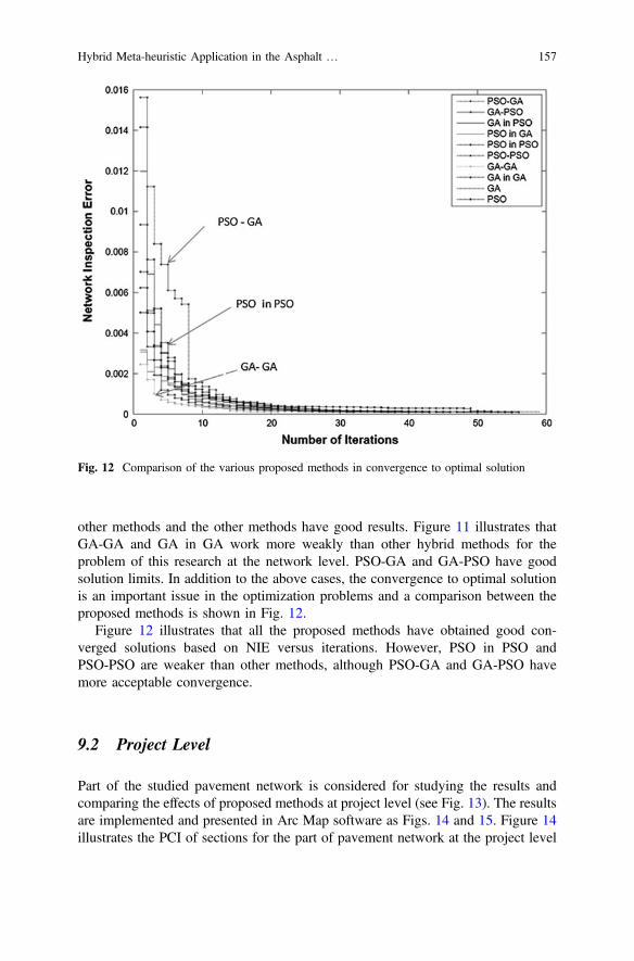
other methods and the other methods have good results. Figure 11 illustrates thatGA-GA and GA in GA work more weakly than other hybrid methods for theproblem of this research at the network level. PSO-GA and GA-PSO have goodsolution limits. In addition to the above cases, the convergence to optimal solutionis an important issue in the optimization problems and a comparison between theproposed methods is shown in Fig. 12.

Figure 12 illustrates that all the proposed methods have obtained good con-verged solutions based on NIE versus iterations. However, PSO in PSO andPSO-PSO are weaker than other methods, although PSO-GA and GA-PSO havemore acceptable convergence.

9.2 Project Level

Part of the studied pavement network is considered for studying the results andcomparing the effects of proposed methods at project level (see Fig. 13). The resultsare implemented and presented in Arc Map software as Figs. 14 and 15. Figure 14illustrates the PCI of sections for the part of pavement network at the project level

Fig. 12 Comparison of the various proposed methods in convergence to optimal solution

Hybrid Meta-heuristic Application in the Asphalt … 157

Fig. 13 Pavement network of district No. 16 of Tehran municipality with the considered part

Fig. 14 PCIs of a considered part of the studied pavement network with proposed methods atproject level (PSO-GA)

158 F. Moghadas Nejad et al.

sampled by the proposed methods and Fig. 15 shows the related SE of sections forthis part. This figure is equal to the differences between Figs. 13 and 14. Figure 15illustrates that the SE of all of the methods is acceptable for the sections of apavement network. The results of the considered part of the studied pavementnetwork is presented and summarized in Fig. 16 for comparing the effect of pro-posed methods.

Figure 16 includes the SE and number of SIUs (NSIUs) with a comparisonbetween the proposed methods by these parameters. This figure illustrates that all ofthe methods have acceptable SEs, and that the PSO-GA, GA-PSO, GA in PSO, andPSO in PSO sampled lower NSIUs than other proposed methods.

Fig. 15 SEs of a considered part of the studied pavement network with proposed method atproject level

Hybrid Meta-heuristic Application in the Asphalt … 159

Fig. 16 Comparison between the proposed methods in SE of the considered part of studiedpavement network. a SE in the considered part of project level. b Number of SIUs in theconsidered part of project level. c SE versus number of SIUs in the considered part

160 F. Moghadas Nejad et al.

10 Conclusions

In this chapter, eight hybrid methods of GA and PSO are proposed with variousapproaches derived for optimal arrangement of the SIUs with accurate PCI in acomprehensive case study of the pavement network in two levels (network andproject levels). This problem is formulated with objectives, including SE and NIE,and is subject to a number of constraints for optimal arrangement of SIUs in thepavement sections of a network.

Finally, these hybrid methods are compared with the PSO and GA alone basedon various cases such as estimation accuracy of PCI, SE, convergence diagrams,TNIE, CPU time, and total number of SIUs.

The major findings of this research are as follows:

• The hybrid methods of PSO and GA have been successful for solving thepresent problem and achieved the least SE in the sections of pavement networkwith optimal arrangement of SIUs. These approaches are better than PSO andGA.

• Selecting the best approach and the comprehensive sampling procedure isaccomplished for obtaining better pavement network analysis. Based on thisissue, PSO-GA is the best approach in the network level that generates betterresults in TNIE, CPU time, and total number of SIUs than other methods initerative runs.

• The proposed methodology of this chapter can help pavement managers andinspectors use optimal decision making in inspection processes and samplingplans with high accuracy, low analysis time, and low number of SIUs.

• The hybrid methods enable us to obviate the analyzing and planning problemsof the inspection process in the pavement network effectively.

• The results show that the proposed methods as well as the sampling process canbe simulated and they work for each number of inspection units in the sectionsand each number of sections in a pavement network better than GA and PSOseparately.

• The proposed hybrid methods have been successful for converging to optimalsolution and work better than singularly.

• One of the challenges of the methods presented in the literature was limitation ininspection unit PCIs spectrum in the sections. The proposed methods are shownto work for each PCI spectrum and have removed this limitation.

• The reliability of results of hybrid methods of PSO-GA and GA-PSO in theiterative runs is better than other methods based on the NIE, total number ofSIUs, and CPU time.

• As the PSO has characteristics such as the simplicity and lack of evolutionaryoperators on the one hand and good convergence of GA with more explorationof solutions by related operators on the other, hybrid approaches of PSO and GAare useful for increasing the potential of solving the present problem. This issueis shown in the results of this research. The convergence of PSO-GA andGA-PSO is better than the other methods.

Hybrid Meta-heuristic Application in the Asphalt … 161

References

1. Medury, A., Madanat, S.: Simultaneous network optimization approach for pavementmanagement systems. J. Infrastruct. Syst. 20(3), 04014010 (2014)

2. Shahnazari, H., Tutunchian, M.A., Mashayekhi, M., Amini, A.A.: Application of softcomputing for prediction of pavement condition index. J. Transp. Eng. 138(12), 1495–1506(2012)

3. Zhou, G., Wang, L.: Co-location decision tree for enhancing decision-making of pavementmaintenance and rehabilitation. J. Transp. Res. Part C 21, 287–305 (2012)

4. Bianchini, A.: Fuzzy representation of pavement condition for efficient pavementmanagement. J. Comput. Aid. Civil Infra. Eng. 27, 608–619 (2012)

5. Meegoda, J., Gao, S.: Roughness progression model for asphalt pavements using long-termpavement performance data. J. Transp. Eng. 140(8), 04014037 (2014)

6. Bogus, S., Song, J., Waggerman, R., Lenke, L.: Rank correlation method for evaluatingmanual pavement distress data variability. J. Infrastruct. Syst. 16(1), 66–72 (2010)

7. Su, Y., Kang, S., Chang, J., Hsieh, S.: Dual-light inspection method for automatic pavementsurveys. J. Comput. Civ. Eng. 27(5), 534–543 (2013)

8. Smilowitz, K., Madanat, S.: Optimal inspection and maintenance policies for infrastructurenetworks. Comput. Aided Civil Infrastruct. Eng. 15(1), 5–13 (2000)

9. Koch, C., Jog, G., Brilakis, I.: Automated pothole distress assessment using asphalt pavementvideo data. J. Comput. Civ. Eng. 27(4), 370–378 (2013)

10. Shahin, M.Y.: Pavement Management for Airports, Roads and Parking Lots, 2nd edn.Springer, New York (2005)

11. Hegazy, T., Elhakeem, A., Ahluwalia, S.S., Attalla, M.: MOST-FIT: support techniques forinspection and life cycle optimization in building asset management. Comput. Aided CivilInfrastruct. Eng. 27, 130–142 (2012)

12. Bianchini, A.: Pavement maintenance planning at the network level with principal componentanalysis. J. Infrastruct. Syst. 20(2), 04013013 (2013)

13. Buddhavarapu, P., Banerjee, A., Prozzi, J.A.: Influence of pavement condition on horizontalcurve safety. J. Accid. Analy. Prevent. 52, 9–18 (2013)

14. Terzi, S.: Modeling for pavement roughness using the ANFIS approach. J. Adv. Eng. Softw.57, 59–64 (2013)

15. Alabama Department of Transportation: A Study of Manual Versus Automated PavementCondition Surveys. Montgomery (2004)

16. Kuhn, K.D.: Pavement network maintenance optimization considering multidimensionalcondition data. J. Infrastruct. Syst. 18(4), 270–277 (2012)

17. Alsugair, A.M., Al-Qudrah, A.A.: Artificial neural network approach for pavementmaintenance. J. Comput. Civ. Eng. 12(4), 249–255 (1998)

18. McPherson, E.G., Muchnick, J.: Effects of street tree shade on asphalt concrete pavementperformance. J. Arboric. 31(6), 303–310 (2005)

19. Galleo, E., Moya, M., Piniés, M., Ayuga, F.: Valuation of low volume roads in Spain. Part 2:Methodology validation. J. Biosys. Eng. 101(1), 135–142 (2008)

20. Li, X., Keegan, K., Yazdani, A.: Index of Foreign Object Damage in Airfield PavementManagement, Transportation Research Record: Journal of the Transportation Research Board,2153, Transportation Research Board of the National Academies, Washington, D.C., pp. 81–87 (2010)

21. Moazami, D., Behbahani, H., Muniandy, R.: Pavement rehabilitation and maintenanceprioritization of urban roads using fuzzy logic. J. Expert Syst. Appl. 38(10), 12869–12879(2011)

22. Tabatabaei, S.A., Khaledi, S., Jahantabi, A.: Modeling the deduct value of the pavementcondition of asphalt pavement by adaptive neuro fuzzy inference system. J. Pave. Res. Tech. 6(1), 59–65 (2013)

162 F. Moghadas Nejad et al.

23. Department of Environment, Heritage and Local Government. (2004). Non-national RoadsCondition Study. Ireland

24. Michigan Department of Transportation: Statewide Pavement Management Report: Phase Oneand Two Airports. Applied Pavement Technology Inc., Illinois (2008)

25. Texas Transportation Institute: Use of Micro Unmanned Aerial Vehicles for RoadsideCondition Assessment. Texas Transportation Institute, Texas (2010)

26. Oregon Department of Aviation: Pavement Evaluation/Maintenance Management Program:Final Report—Individual Airports Functional Category 2. Pavement Consultants Inc.,Washington (2011)

27. ASTM D6433-11: Standard Practice for Roads and Parking Lots Pavement Condition Index.ASTM international, West Conshohocken (2011)

28. De la Garza, J.M., Piñero, J.C., Ozbek, M.E.: Sampling procedure for performance-based roadmaintenance evaluations. Transp. Res. Rec.: J. Transp. Res. Board 2044, 11–18 (2008)

29. Mishalani, R.G., Gong, L.: Optimal infrastructure condition sampling over space and time formaintenance decision-making under uncertainty. J. Transp. Res. Part B 43(3), 311–324 (2009)

30. Talbi, El: Metaheuristics: from Design to Implementation, 1st edn. Wiley, New Jersey (2009)31. Miradi, M., Molenaar, A.A., van de Ven, F.C.: Knowledge discovery and data mining using

artificial intelligence to unravel porous asphalt concrete in the Netherlands. In:Gopalakrishnan, K., et al. (eds.) Intelligent and Soft Computing in Infrastructure SystemsEngineering, SCI, vol. 259, pp. 107–176 (2009)

32. Adeli, H.: Neural networks in civil engineering: 1989-2000. Comput.-Aided Civil Infrastruct.Eng. 16, 126–142 (2001)

33. Tack, J.N., Chou, E.Y.J.: Multiyear pavement repair scheduling optimization bypreconstrained genetic algorithm. Transp. Res. Rec.: J. Transp. Res. Board 1816, 3–8 (2002)

34. Chan, W.T., Fwa, T.F., Tan, J.Y.: Benefits of information integration in budget planning forpavement management. Transp. Res. Rec.: J. Transp. Res. Board 1889, 3–12 (2004)

35. Maji, A., Jha, M.K.: Modeling highway infrastructure maintenance schedule with budgetconstraint, TRB Annual Metting, Transportation Research Board of the National Academies,Washington, D.C (2007)

36. Tang, Y., Chien, S.I.: Scheduling Work Zones for Highway Maintenance Projects Consideringa Discrete Time-Cost Relation, Transportation Research Record: Journal of the TransportationResearch Board, 2055, pp. 21–30. Transportation Research Board of the National Academies,Washington, D.C. (2008)

37. Gosse, C.A., Smith, B.L., Clarens, A.F.: Environmentally preferable pavement managementsystems. J. Infrastruct. Syst. 19(3), 315–325 (2013)

38. Kepaptsoglou, K., Konstantinidou, M., Karlaftis, M.G., Stathopoulos, A.: Planningpost-disaster operations in a highway network: a 1 network design model withinterdependencies, TRB Annual Metting, Transportation Research Board of the NationalAcademies, Washington, D.C (2014)

39. Clerc, M., Kennedy, J.: The particle swarm-explosion, stability, and convergence in amultidimensional complex space. IEEE Trans. Evol. Comput. 6(1), 58–73 (2002)

40. Lotfi, M.M., Tavakkoli-Moghaddam, R.: A genetic algorithm using priority-based encodingwith new operators for fixed charge transportation problems. J. Appl. Soft Comput. 13(5),2711–2726 (2013)

41. Cavuoti, S., Garofalo, M., Brescia, M., Paolillo, M., Pescape’, A., Longo, G., Ventre, G.:Astrophysical data mining with GPU. A case study: genetic classification. J. New Astro. 26,12–22 (2014)

42. Lu, P., Tolliver, D.: Multiobjective pavement-preservation decision making with simulatedconstraint boundary programming. J. Transp. Eng. 139(9), 880–888 (2013)

43. Gopalakrishnan, K.: Neural network-swarm intelligence hybrid nonlinear optimizationalgorithm for pavement moduli back-calculation. J. Transp. Eng. 136(6), 528–536 (2010)

44. Chang, J.: Particle swarm optimization method for optimal prioritization of pavement sectionsfor maintenance and rehabilitation activities. Appl. Mech. and Mat. 343, 43–49 (2013)

Hybrid Meta-heuristic Application in the Asphalt … 163

45. Tayebi, N.R., Moghadas Nejad, F., Mola, M.: Comparison between GA and PSO in analyzingpavement management activities. J. Transp. Eng. 140(1), 99–104 (2014)

46. Blum, C., Roli, A.: Hybrid Metaheuristics: An Introduction, Studies in ComputationalIntelligence(SCI), vol. 114, pp. 1–30. Springer, New York (2008)

47. Greene, J., Shahin, M.Y., Alexander, D.R.: Airfield Pavement Condition Assessment,Transportation Research Record: Journal of the Transportation Research Board, No. 1889,TRB, National Research Council, Washington, D.C., pp. 63–70 (2004)

48. Moghadas Nejad, F., Zakeri, H.: The hybrid method and its application to smart pavementmanagement. In: Yang, X. S., Alavi, A. H., (eds.) Metaheuristics in Water, Geotechnical andTransport Engineering, pp. 439–484 (2013)

49. Kennedy, J., Eberhart, R.C.: Particle swarm optimization. Proceedings of IEEE InternationalConference on Neural Networks, vol. 4, pp. 1942–1948, Piscataway, N.J. (1995)

50. Kuoa, R.J., Lin., L.M.: Application of a hybrid of genetic algorithm and particle swarmoptimization algorithm for order clustering. J. Dec. Supp. Sys. 49, 451–462 (2010)

51. Clerc, M.: The swarm and the queen: towards a deterministic and adaptive particle swarmoptimization. In: Proceedings of IEEE Congress on Evolutionary Computation, pp. 1951–1957 (1999)

52. Parsopoulos, K.E., Vrahatis, M.N.: Recent approaches to global optimization problemsthrough particle swarm optimization. Nat. Comput. 1, 235–306 (2002)

53. Robinson, J., Rahmat-Samii, Y.: Particle swarm optimization in electromagnetics. IEEE Trans.Antennas Propag. 52(2), 397–407 (2004)

54. Kennedy, J., Eberhart, R.C.: A discrete binary version of the particle swarm algorithm. In:Proceedings of IEEE International Conference Systems, Man and Cybernetic. IEEE ServiceCenter, Piscataway, NJ, pp. 4104–4108 (1997)

55. Lipowski, A., Lipowska, D.: Roulette-wheel selection via stochastic acceptance. J. Phys.A 391(6), 2193–2196 (2012)

56. Lu, Ch., Yu, V.F.: Data envelopment analysis for evaluating the efficiency of geneticalgorithms on solving the vehicle routing problem with soft time windows. J. Comput. Indust.Eng. 63(2), 520–529 (2012)

57. Sivanandam, S.N., Deepa, S.N.: Introduction to Genetic Algorithms, 1st edn. Springer, Berlin(2008)

58. Kao, Y.T., Zahara, E.: A hybrid genetic algorithm and particle swarm optimization formultimodal functions. Appl. Soft Comput. 8(2), 849–857 (2008)

59. Zeng, K., Peng, G., Cai, Z., Huang, Z., Yang, X.: A hybrid natural computing approach for theVRP problem based on PSO, GA and quantum computation. In: Yeo, S.-S., et al. (eds.)Computer Science and Its Applications. Springer Science+Business Media, Dordrecht (2012)

60. Castillo, O.: Type-2 Fuzzy Logic in Intelligent Control Applications: A Hybrid PSO-GAOptimization Method to Design Type-1 and Type-2 Fuzzy Logic Controllers, STUDFUZZ272, pp. 105–118. Springer, Heidelberg (2012)

61. Kumar, P.G., Victoire, T.A., Renukadevi, P., Devaraj, D.: Design of fuzzy expert system formicroarray data classification using a novel Genetic Swarm Algorithm. Expert Syst. Appl. 39(2012), 1811–1821 (2012)

62. Babu, K., Vijayalakshmi, D.: Self-Adaptive PSO-GA hybrid model for combinatorial waterdistribution network design. J. Pipeline Syst. Eng. Pract. 4(1), 57–67 (2013)

63. Martínez-Soto, R., Castillo, O., Aguilar, L.T., Rodriguez, A.: A hybrid optimization methodwith PSO and GA to automatically design Type-1 and Type-2 fuzzy logic controllers, Int.J. Mach. Learn. Cybern. (2013)

64. Galvez, A., Iglesias, A.: A new iterative mutually coupled hybrid GA–PSO approach for curvefitting in manufacturing. Appl. Soft Comput. 13, 1491–1504 (2013)

164 F. Moghadas Nejad et al.

Optimum Reinforced Concrete Designby Harmony Search Algorithm

Gebrail Bekdaş, Sinan Melih Nigdeli and Xin-She Yang

Abstract The music-inspired metaheuristic method, called harmony search (HS),is an effective tool in optimization of engineering design problems. HS has beenapplied for the optimum design of reinforced concrete (RC) members so as to findthe best solution, balancing the usability of the design and economy. In this chapter,the optimum design of RC members is presented after optimization of RC mem-bers. Then, HS-based optimization applications, such as RC slender columns, RCshear walls, and post-tensioned RC axially symmetric cylindrical walls, are alsodiscussed. The HS-based methods are feasible in finding the optimum design insuch problems.

Keywords Metaheuristic methods � Reinforced concrete � Optimization �Harmony search algorithm

1 Introduction

A structural system excited by external forces is under the effect of tensile andcompressive stresses. By using brittle materials, like stone bricks, mud brick kiln,and concrete, it will not be possible to construct a structure resisting tensile stresses.These types of materials are effective with their compressive strength, while their

G. Bekdaş � S.M. NigdeliDepartment of Civil Engineering, Istanbul University,34320 Avcılar, Istanbul, Turkeye-mail: bekdas@istanbul.edu.tr

S.M. Nigdelie-mail: melihnig@istanbul.edu.tr

X.-S. Yang (&)Design Engineering and Mathematics, Middlesex University London,The Burroughs, London NW44BT, UKe-mail: x.yang@mdx.ac.uk; xy227@cam.ac.uk

© Springer International Publishing Switzerland 2016X.-S. Yang et al. (eds.), Metaheuristics and Optimization in Civil Engineering,Modeling and Optimization in Science and Technologies 7,DOI 10.1007/978-3-319-26245-1_8

165

tensile strength of the materials is nearly zero. In that case, ductile materials likesteel may be used in construction, but the major disadvantages of steel are its highcosts and environmental factors. This situation leads us to use composite structuresin which two materials with different mechanical behavior are used together. Forthat reason, optimization is essential in design. Reinforced concrete (RC) structuresare the structures using concrete as a form of the whole structure and that form isreinforced with steel bars where tensile stresses occur. In these structures, steel isonly used as slender bars while its stability and protection from environmentalfactor are supported by the concrete covering the bars. The cost minimizationproblem of RC members has been investigated in several studies. The most chal-lenging issue in RC design is to provide the ductile fracture of concrete. When thefracture is brittle, it will be not possible to absorb huge energy. Thus, the designprocedure of RC elements is nonlinear and it is not possible to estimate the bestdesign with the minimum cost. Also, steel bars with fixed sizes in the market andorientation must be suitable for force transfer by forming a bond between steel andconcrete. Because of these reasons, numerical iteration methods are more suitablethan mathematical ones in the optimum design of RC members.

In finding the optimum design variables of RC members, metaheuristic methodsare very suitable. Genetic algorithm (GA) has been employed in several approa-ches. Coello et al. [1] developed a GA-based approach for RC beams. GA is alsoused in the methodology of Rafiq and Soutcombe [2] in which biaxial RC columnsare optimized. Another study employing GA is the RC design study of Koumousisand Arsenis [3], investigating different types of structural members. Rajaev andKhrisnamoorthy optimized frame structures consisting of RC beam and columnmembers by using GA-based method [4]. Rath et al. [5] used GA in cost opti-mization while sequential quadratic programing technique is employed in the shapeoptimization of RC members. Camp et al. investigated the slenderness effect of RCcolumn in the optimization study proposed by for RC frames employing GA [6].T-shaped beams, investigated together with the effective slab length on the top ofthe beams are optimized by Ferreira et al. [7] and different design codes arechecked.

GA is one of the oldest metaheuristic algorithms and studies combined GA withother methods in their search for the best optimum results. It has been combinedwith simulated annealing (SA) in order to optimize continuous beams by Leps andSejnoha [8]. By using a design database, GA was employed in the design of RCframes by Lee and Ahn [9].

Balling and Yao [10] developed a methodology for three dimensional RC framessubjected to different types of loads, such as dead, live, snow, and earthquake.Ahmadkhanlou and Adeli [11] investigated RC slabs by using a methodology withtwo stages. In the first stage of methodology, the neural dynamics model [12, 13]developed by Adeli and Park is used in order to find the optimum solution ofcontinuous variables and then, perturbation technique is used on modification of theoptimum values to practical ones. Several optimization expressions related with the

166 G. Bekdaş et al.

bending moment, steel area, and ratio of singly or doubly RC beams were devel-oped by Barros et al. [14]. Sirca Jr. and Adeli investigated the minimum costoptimization of prestressed concrete bridges [15]. Govindaraj and Ramasamy [16]optimized continuous beams by selecting design variables from a typical databaseof reinforcement template. Sahab et al. hybridized GA with the discretized form ofHook and Jeeves method for optimization of RC flat slab building [17]. Staticallyloaded RC frames were optimized by using GA-based method by Govindaraj andRamasamy [18]. Optimization of multi-bay single-story and single-bay multi-storyRC frames are done by Guerra and Kiousis [19].

Simulated annealing (SA) is also a widely employed algorithm in RC designoptimization. Paya et al. [20] employed SA in RC frame optimization. SA is alsoused as a part in the methodology of Perea et al. [21]. In this research, RC frames ofbridges were optimized by using SA with a metaheuristic called threshold acceptingand two heuristic methods such as random walk and descent local search. SA is alsoemployed in the RC frame optimization study considering the minimization of thevalue of embedded CO2 emission by Paya-Zaforteza et al. [22]. Also, Camp andHuq employed big bang big crunch algorithm (BB-BC) for the CO2 emissionminimization of RC frames [23].

A reinforcement sizing diagram was provided for RC beams and columns byGil-Martin et al. [24]. The optimum depth and reinforcement design of rectangularRC beams was investigated by Barros et al. [25]. Fedghouche and Tiliouine opti-mized T-shaped RC beam by employing GA and the study only covers the designof beams without steel bars under compressive forces [26].

The optimum design of RC retaining walls is also challenging because stabilityof the wall subjected to soil load must be ensured. This security is generallyprovided by increasing the weight of the wall, but in that case, the internal forcesincrease and the economy cannot be provided. For that reason, a balanced optimumdesign must be found and metaheuristic methods, such as SA [27, 28], harmonysearch (HS) [29], BB-BC [30], and charged system search (CSS) [31] have beensuccessfully employed for optimization of RC retaining walls.

HS algorithm has also been employed for optimum RC members, such ascontinuous beams [32], T-shaped beams [33], columns [34, 35], frames [36], shearwalls [37], cylindrical walls [38], post tensioning cylindrical walls [39], and biaxialcolumns [40]. Kaveh and Sabzi used the combination of several metaheuristic in theoptimum design of RC frames [41]. BB-BC-based RC beam optimization wasdeveloped by Kaveh and Sabzi [42]. SA and Tabu search were combined in order todevelop an optimum design methodology for hybrid fiber reinforced compositeplates by Rama Mohan Rao and Shyju [43]. Nigdeli and Bekdaş developed arandom search technique in optimization of RC beams [44]. Bekdaş and Nigdelioptimized uniaxial RC beam by using random search technique [45, 46]. Jahjouhet al. investigated continuous beams by employing Artificial Bee Colony(ABC) [47].

Optimum Reinforced Concrete Design by Harmony Search Algorithm 167

2 Harmony Search Algorithm

As designers searching for the optimum design, a musician also has a primary goal,which is to achieve the harmony of the music and thus, the admiration of theaudience. The Harmony Search (HS) algorithm is a music-inspired algorithm,developed by Geem et al. [48]. HS is a memory-based random search method. Inthe musical performances, musicians try to find a pleasing harmony and this har-mony is a perfect state of music performance. Similarly, researchers try to find aglobal solution (a good, ideally, optimal solution of all design variables) for min-imizing or maximizing an objective function (or objective functions inmulti-objective optimization). HS uses a stochastic random search instead of agradient search. HS was extended to solve both discrete variable [49] and contin-uous variable [50] problems.

The HS method can be briefly explained in five steps for design problems.

i. In the first step, constant values of the optimization problem are defined. Thesevalues are solution ranges of design variables, specific parameters of HS algo-rithm, and design problem constants. The solution ranges are defined in order tofind the solution quickly by tightening the range or preventing several solutiondomains for design constraints or practical design. The algorithm parameters areharmonymemory size (HMS), harmonymemory considering rate (HMCR), andpitch adjusting rate (PAR). Additionally, the HS algorithmwas also improved inorder to develop parameter setting free techniques [51, 52].

ii. Before using the properties of the algorithm, an initial harmony memory(HM) matrix is constructed and it contains harmony vectors. The parameter;HMS is the number of harmony vectors in HM and a harmony vector includesa set of design variables, which are randomly generated by using the solutionranges defined in the first step. Also, the optimization objective or objectivesare defined for each set of design variables. The formulation must contain theconsideration of design constraints if the constraints are violated. In designproblems, design constraints are generally seen and the exiting of these con-straints may be the reason of using numerical optimization methods.

iii. In this step, the optimization starts. A new harmony vector is defined by usingthe special rules of HS. In musical performances, musicians play a randomnotes and this note may be a current popular song. In that case, a musicianmay slightly chance this note in order to gain admiration by playing notessimilar to current best. Or maybe, a musician may try to play a new melody ina performance. Musicians must use these two options. Otherwise, they maylose their popularity if they do not produce a novel work. In optimum design,we need to search the best result around the current best solution in order toimprove the convergence of the method, but the solution should not be a localoptimum, though there is no guarantee. For that reason, we need to generatenew solutions by using randomization in the whole domain. A new vector isgenerated around the existing ones in HM or from the initial range. The valueof HMCR controls the type of the generation and it is the possibility of the

168 G. Bekdaş et al.

generation done by using an existing vector in HM. The neighboring values ofa chosen vector may be defined by using a smaller solution range. Theparameter; PAR is used to reduce the solution area of design variables. Theratio of the small range and initial range can be defined with the value of PAR.The limits of the design variables should also be applied to ensure the solutionranges. If the chosen vector is near to the bounds of solution ranges, the designvariables may be assigned with the values out of the range.

iv. In this step, the newly generated harmony vector is selected or not. It iscompared with the current worst vector in mean of minimization or maxi-mization of objective functions. If the new one is better than the worst one, thenew solution is stored by eliminating the worst one. Thus, the harmonymemory is updated.

v. In the last step, the termination criterion or criteria are changed. Until thistermination criterion is provided, the optimization process continues from thethird step. The termination criterion may be a fixed number of iterations orconvergence of the design variables. It is possible to use several terminationcriteria in design problems.

3 Optimum Design Examples

In this section, three applications of RC design members are presented byemploying the HS algorithm. The problems are the optimization of slender RCcolumns, optimization of RC shear walls, and optimum design of post-tensionedRC axially symmetric cylindrical walls.

3.1 Optimum Design of Slender RC Columns

In a structural system, columns are generally under the effect of axial forces. Due tothe deflection of columns under external loads, second-order effects occur, andslenderness and buckling of the columns is the reason of this issue. Slenderness andbuckling stress can be affected by the length of the column, cross-sectionaldimensions and effective length factor in buckling (k) of columns. In this example,HS is employed by considering the regulations of ACI318 (Building CodeRequirements for Structural Concrete) [54].

In ACI318, slenderness effects are considered by using the approximate designprocedure in which the flexure moment on the column is magnified with momentmagnification factor (δs). In this procedure, the moments of inertia of beams andcolumns are, respectively, reduced with 65 and 30 % because of consideration ofcracking. Subject to the ductile design, cracking of the beam is more possible thancolumns and, for that reason, the reduction of the moments of inertia of beams can

Optimum Reinforced Concrete Design by Harmony Search Algorithm 169

be big. Effective length factors in buckling (k) are found according ratio; Ψ cal-culated at both ends of columns (ΨA; upper end—ΨB; lower end). In the equation ofthis ratio, E, I, and l are elasticity modulus, moment of inertia, and the length of thecorresponding RC members, respectively, as seen in Eq. (1).

WA;B ¼P

EI=lð ÞcolumnPEI=lð Þbeam

ð1Þ

After ΨA and ΨB are calculated, k is obtained from the set of equations given asEq. (2). These equations are for structural systems which are free in horizontaldirection.

Wm ¼ 0:5ðWA þWBÞk ¼ 20�Wm

20

ffiffiffiffiffiffiffiffiffiffiffiffiffiffiffi1þWm

pif Wm\2

k ¼ 0:9ffiffiffiffiffiffiffiffiffiffiffiffiffiffiffi1þWm

pif Wm � 2

9>>>=>>>;

ð2Þ

The moment magnification factor (δs) is calculated as

ds ¼ Cm

1� Pu0:75Pc

ð3Þ

where Cm is the correction factor which considers the actual moment diagram to anequivalent uniform moment diagram. It can be calculated as

Cm ¼ 0:6þ 0:4M1

M2ð4Þ

and Cm must be bigger than 0.4, while it is 1.0 for members with transverse loadsbetween supports. In Eq. (3), critical buckling load is calculated as

Pc ¼ p2EI

ðklÞ2 ð5Þ

by reducing the rigidity of the column by 75 %.The design variables of the problem are the dimensions of the column and

amount of reinforcements (both longitudinal and shear). The column is underloadings, such as flexural moment (M), shear force (V), and axial force (N). Thedesign constants are clear cover of concrete (cc), maximum aggregate diameter(Dmax), length of column (l), elasticity modulus of steel (Es), cost of the concrete perm3 (Cc), cost of the steel per ton (Cs), compressive strength of concrete f 0c

� �, yield

strength of steel (fy), specific gravity of steel (γs), and specific gravity of concrete(γc) are defined.

170 G. Bekdaş et al.

After the cross-section dimensions are randomized, ductility conditions given inEqs. (6) and (7) are checked. Ac is the area of the cross section of columns.

V\0:2f 0cAc

5:5Ac

(ð6Þ

N\0:5f 0cAc ð7Þ

If the element is under brittle fracture risks, the cross-sectional dimensions areupdated before the randomization of reinforcements are done. Thus, the designconstraints, given as Eqs. (6) and (7), are considered and the computation time issaved. Then, the number and size of reinforcement bars are done and placementconditions are checked. If the placement requirements given in ACI318;

a/ [

1:5/avarage

40 mm43Dmax

8>>><>>>:

ð8Þ

is not provided, reinforcements are updated by also considering a design with twolines. ϕaverage is the average of the diameter sizes and aϕ is the clear distancebetween reinforcement bars. Similarly, as done in ductility conditions, the rein-forcements are iteratively randomized if the placement conditions are not provided.

In order to conduct a design for axial forces and magnified flexural moments, adesign methodology using random searches is conducted in production of harmonyvectors. The distance from extreme compressive fiber to neural axis (c) is iterativelyscanned for the best flexural moment and axial force combination. For the requiredaxial force, the corresponding flexural moment capacity is found. This flexuralmoment capacity must be close and higher than the required one. The difference ofthe percentage may be defined as a function of the iteration number. Thus, thesolutions far from the optimum are quickly eliminated.

After the design for axial force and magnified flexural moment, the design ofshear reinforcements is done by iteratively assigning diameter sizes. The requireddistance of shear reinforcement (stirrups) is calculated for all iterations. Then, thenominal shear strength of concrete (Vc) and nominal shear strength of reinforce-ment (Vs) are calculated as given in Eqs. (9) and (10), respectively.

Vc ¼ffiffiffiffif0c

q

6bwd ð9Þ

Vs ¼ Avfyds

ð10Þ

Optimum Reinforced Concrete Design by Harmony Search Algorithm 171

where Av represents the area of shear reinforcement spacing s. The effective depthof the column is defined with d. Additionally, the Vs value must be lower than

0:66ffiffiffiffif0c

qbwd. If this constraint and total shear strength of the column is lower than

the required one, the objective function is penalized. Also, the calculated resultsmust be higher than the minimum shear reinforcement (Av,min) value and the dis-tance between the bars must be lower than the maximum shear reinforcementdistance (smax) given in Eqs. (11) and (12), respectively

Avð Þmin¼13bwsfy

ð11Þ

smax

� d4

if Vs � 0:33ffiffiffiffif 0c

qbwd

� d2

otherwise:

8><>:

ð12Þ

The total material cost of design (C), which is the main objective of the problem,is also stored in the harmony vectors. The elimination of the worst solutions is doneaccording to the same objective function given in Eq. (13). The optimizationprocess is done for the maximum iteration number. As, ust, γs, Cc, and Cs are thearea of non-prestressed longitudinal reinforcement, the length of shear reinforce-ment spacing s, the specific gravity of steel, the material cost of the concrete per m3

and the material cost of the steel per ton, respectively.

min C ¼ ðAc � AsÞCcþ ðAs þ Av

sustÞlcsCs ð13Þ

The loading at the upper end of the column such as axial force, flexural moment,and shear force were taken as 2000 kN, 50 kNm, and 50 kN, respectively. Designconstants are taken as given in Table 1.

Optimum design variables are investigated by using k values between 0.5 and2.0. The optimum results are presented in Table 2. The slenderness effects are noteffective for columns with an effective length factor in buckling (k) lower than 1.3.In that situation, the optimum values are equal for all. Then, parallel to k, theincrease of the cost is seen.

3.2 Optimum Design of RC Shear Walls

In this example, RC shear walls are presented for optimum design considering thetotal cost minimization and the design methodology is done according to ACI 318[53]. The optimum design is scanned by randomizing the design variable show inFig. 1. The design variables are breadth of the shear wall (bw), reinforcements in

172 G. Bekdaş et al.

columns headings and web of the shear walls. All reinforcements including thestirrups are defined with a diameter size in mm and a distance between each bars inmm. The proposed methodology can be by the following steps.

First step: As similarly for all design optimization problems, design constantsshown in Table 3, the ranges of design variables (also shown in Table 3), specialharmony search parameters explained in the second section and the design internalforces of the RC shear walls (as given in Table 4) are defined.

Table 1 The design constants of column example

Definition Symbol Unit Value

Range of the breadth bw mm 250–400

Range of the height h mm 300–600

Length l mm 4500

Clear cover cc mm 30

Range of reinforcement ϕ mm 16–30

Range of shear reinforcement ϕv mm 8–14

Max. aggregate diameter Dmax mm 16

Yield strength of steel fy MPa 420

Comp. strength of concrete f 0c MPa 25

Elasticity modulus of steel Es MPa 200000

Specific gravity of steel γs t/m3 7.86

Cost of the concrete per m3 Cc $ 40

Cost of the steel per ton Cs $ 400

Table 2 Optimum results for column example

k 0.5–1.2 1.3 1.4 1.5 1.6 1.7 1.8 1.9 2.0

Breadth ofcolumn (bw)(mm)

300 300 300 300 300 300 350 350 350

Height ofcolumn(h) (mm)

550 550 600 600 600 600 600 600 600

Bars in eachface

1Φ18+1Φ16

3Φ16 2Φ16 2Φ16 2Φ16 2Φ16+1Φ18

1Φ20+1Φ18

1Φ20+1Φ18

4Φ16

Webreinforcements

2Φ16 2Φ16 2Φ18 2Φ18 2Φ18 2Φ16 2Φ18 2Φ18 2Φ16

Shearreinforcementdiameter (mm)

Φ8 Φ8 Φ8 Φ8 Φ8 Φ8 Φ8 Φ8 Φ8

Shearreinforcementdistance (mm)

240 240 270 270 270 270 270 270 270

Optimum cost($)

58.764 62.889 62.972 62.972 62.972 67.097 73.308 73.308 76.906

Optimum Reinforced Concrete Design by Harmony Search Algorithm 173

Second step: The generations of harmony vectors are done in three substepsnamed as steps a, b, and c. In these steps, iterative randomization is done in order toensure the ACI 318 requirements.

Step a: The breadth (bw) of the shear wall is randomized and ductility conditionsgiven in Eqs. (6–7) are checked. The randomization of bw continues until theductility conditions are met. Also, some discrete randomization is carried out inorder to assign values which are the multiples of 50 mm. In the construction yard, asensible production of cross-section dimensions is not possible.

Step b: Then, the reinforcements are randomized by checking the capacity of theshear wall. The reinforcements at the column headings and web are separatelyrandomized. For the design shear force (V), shear reinforcement (stirrup) design isalso carried out by the procedure given in the RC column example.

Step c: In the last substep, the distance from extreme compressive fiber to neuralaxis (c) is iteratively searched in order to find the best flexural moment and axialforce combination. The stress on each bar is calculated and the force equilibrium is

b wstirrups in column headings

reinforcements in column headings

web reinforcements

stirrups in web

Fig. 1 Design variables of RC shear wall

Table 3 The design constants and solution ranges of RC shear wall example

Definition Symbol Unit Value in example

Range of the breadth bw mm 250–600

Height h mm 3000

Length l mm 4000

Clear cover cc mm 30

Range of reinforcement ϕ mm 16–30

Range of shear reinforcement ϕv mm 8–14

Max. aggregate diameter Dmax mm 16

Yield strength of steel fy MPa 420

Comp. strength of concrete f 0c MPa 25

Elasticity modulus of steel Es MPa 200000

Specific gravity of steel γs t/m3 7.86

Specific gravity of concrete γc t/m3 2.5

Cost of the concrete per m3 Cc $/m3 40

Cost of the steel per ton Cs $/t 400

174 G. Bekdaş et al.

provided in the calculation of the capacity of the shear wall. The stress on concretesection is calculated by assuming an equaling rectangular stress block as explainedin ACI 318. The same procedure with the first example is carried out in order to findthe best suitable design ensuring the axial force and the flexural moment capacity.Finally, the total material cost of the shear wall is calculated and the cost ispenalized, if the flexural capacity of the design is lower than the required one afterseveral randomizations. In that case, the breadth of the design may be too small forthe design forces.

By using the three substeps including random searches, the optimization isdecreased by eliminating the results far from the optimum one. Thus, it is notneeded to use previously generated templates for reinforcement design. Generally,the final results in harmony vectors are good designs which are physically possiblesolutions and close to optimum design. By using the rules of HS, the best one issearched in the third step.

Third step: In this step, the initial harmony memory matrix is updated by usingthe rules of HS. The three substeps are also used in the generation of new harmonyvectors.

Last step: The stopping criterion is the maximum number of iterations. When thenumber of iterations reaches to the maximum iteration number defined by the user,the optimization process is terminated. The maximum iteration number is 2000 forthree loading cases, as given in Table 4.

The optimum design variables are given in Table 5. From the results, theimportance of optimization is clearly seen that the optimum design variables are faraway from the lower and upper bounds of the solution ranges. Concrete is a cheapermaterial than steel, but the optimum reinforcements are not at the minimum limit.For that reason, the required optimum with a balance between both materials isfound and the RC shear wall design with metaheuristic methods is a feasibleapproach.

Table 4 Internal forces forthree cases of RC shear wall

Axialforce[N (kN)]

Flexuralmoment[M (kNm)]

Shear force [V (kN)]

Case 1 500 25 100

Case 2 1000 50 200

Case 3 2000 100 400

Table 5 Optimum design variables of RC shear wall

Cases bw(mm)

Reinforcementsat the columnheading

Webreinforcements ofcolumn heading

Webreinforcementof shear wall

Stirrups Cost ($)

1 250 1Φ20 + 1Φ16 1Φ18 + 1Φ16 3Φ18 + 1Φ16 Φ10/160 232.2871

2 300 1Φ26 + 1Φ22 3Φ16 1Φ18 + 3Φ16 Φ10/120 295.9118

3 450 1Φ18 + 1Φ16 1Φ18 + 1Φ16 2Φ18 + 2Φ16 Φ8/110 324.2167

Optimum Reinforced Concrete Design by Harmony Search Algorithm 175

3.3 Optimum Design of Cylindrical Walls

For the third example, cost optimization of post-tensioned RC axially symmetriccylindrical walls are presented. A typical cylindrical wall model can be seen inFig. 2. The optimization process can be summarized in three stages; static analyses,RC design/cost calculation, and comparison/elimination.

Static analyses: After defining the geometry (height: H and radius of wall: r) ofwall, specific weight of the liquid, design constant, such as, material cost ofmaterial, workmanship, yield strength of steel, parameters of HS algorithm, anddesign variables intensities (P1, P2…, Pn) and locations (a1, a2…, a), thickness ofwall (h), compressive strength of concrete (f΄c), the structural analyses are done byusing the superposition method [54] to obtain internal forces, flexural moments,shear force, and axial tension.

RC design and cost calculations: In this stage, design constraints; flexuralmoment capacities in both direction, shear strength capacity, axial tension, mini-mum steel ratios, minimum and maximum bar spacing, maximum crack width arechecked by considering the diameter of horizontal (ϕh), and vertical (ϕv) bars andbar spacings in both direction (Sh and Sv) as design variables. By providing safetyand applicable solution, the total cost of the wall as objective function of process iscalculated as

min f ðXÞ ¼ CcVc þCsWs þCptWpt þCfwAfw ð14Þ

h

r

H

P1

Pn

P1

Pn

r

h

Pi Pi

an

ai

a1 a1

ai

an

Sh

hφ

Fig. 2 Model of cylindrical wall used in optimization process

176 G. Bekdaş et al.

where

Vc ¼ pH ðrþ h2Þ2 � ðr � h

2Þ2

� �ð15Þ

Ws ¼ p/2v

44prSv

� �Hcs þ

p/2h

42HSh

� �2prcs ð16Þ

Wpt ¼pPn

i¼1 ð/ptÞ2i4

2prcs ð17Þ

Afw ¼ 2pHð2rÞ ð18Þ

Comparison and elimination: In this stage, comparisons and eliminations aredone according to rules of HS algorithm.

The optimization process is performed for five different wall models with dif-ferent heights considering with and without post-tensioning (P-T). Comparing theresults given in Fig. 3, although being limited difference between the costs for 6 mand 8 m wall heights (0.09 % and 1.42 %), by increasing wall height as well asloads, the effects of post-tensioning loads can be clearly seen (4.05 % and 6.55 %).

4 Conclusion

In this chapter, we have described the optimum designs of RC members using HSsearch. The objective function and complex constraints have been formulated foreach case study. Numerical experiments have been carried out and results have beenanalyzed.

20.0

30.0

40.0

50.0

60.0

70.0

80.0

6.0 7.0 8.0 9.0 10.0 11.0 12.0

Tot

al c

ost/1

00 (

$)

Height of wall (m)

Without P-T

With P-T

Fig. 3 The optimum results of the cylindrical wall

Optimum Reinforced Concrete Design by Harmony Search Algorithm 177

From the above examples, we can see that HS can be a good tool to providedesigns with quality solutions that can be used in practical applications. Obviously,it would be useful to see how other algorithms perform and make a detailedcomparison for these types of problems.

References

1. Coello, C.C., Hernandez, F.S., Farrera, F.A.: Optimal design of reinforced concrete beamsusing genetic algorithms. Expert Syst. Appl. 12, 101–108 (1997)

2. Rafiq, M.Y., Southcombe, C.: Genetic algorithms in optimal design and detailing of reinforcedconcrete biaxial columns supported by a declarative approach for capacity checking. Comput.Struct. 69, 443–457 (1998)

3. Koumousis, V.K., Arsenis, S.J.: Genetic algorithms in optimal detailed design of reinforcedconcrete members. Comput-Aided Civ. Inf. 13, 43–52 (1998)

4. Rajeev, S., Krishnamoorthy, C.S.: Genetic algorithm-based methodology for designoptimization of reinforced concrete frames. Comput-Aided Civ. Inf. 13, 63–74 (1998)

5. Rath, D.P., Ahlawat, A.S., Ramaswamy, A.: Shape optimization of RC flexural members.J. Struct. Eng.-ASCE 125, 1439–1446 (1999)

6. Camp, C.V., Pezeshk, S., Hansson, H.: Flexural design of reinforced concrete frames using agenetic algorithm. J. Struct. Eng.-ASCE 129, 105–111 (2003)

7. Ferreira, C.C., Barros, M.H.F.M., Barros, A.F.M.: Optimal design of reinforced concreteT-sections in bending. Eng. Struct. 25, 951–964 (2003)

8. Leps, M., Sejnoha, M.: New approach to optimization of reinforced concrete beams. Comput.Struct. 81, 1957–1966 (2003)

9. Lee, C., Ahn, J.: Flexural design of reinforced concrete frames by genetic algorithm. J. Struct.Eng.-ASCE 129(6), 762–774 (2003)

10. Balling, R., Yao, X.: Optimization of reinforced concrete frames. J. Struct. Eng.-ASCE 123,193–202 (1997)

11. Ahmadkhanlou, F., Adeli, H.: Optimum cost design of reinforced concrete slabs using neuraldynamics model. Eng. Appl. Artif. Intell. 18(1), 65–72 (2005)

12. Adeli, H., Park, H.S.: Optimization of space structures by neural dynamics. Neural Netw. 8(5),769–781 (1995)

13. Adeli, H., Park, H.S.: Neurocomputing for Design Automation. CRC Press, Boca Raton(1998)

14. Barros, M.H.F.M., Martins, R.A.F., Barros, A.F.M.: Cost optimization of singly and doublyreinforced concrete beams with EC2-2001. Struct. Multidiscip. O. 30, 236–242 (2005)

15. Sirca Jr, G., Adeli, H.: Cost optimization of prestressed concrete bridges. J. Struct. Eng. ASCE131(3), 380–388 (2005)

16. Govindaraj, V., Ramasamy, J.V.: Optimum detailed design of reinforced concrete continuousbeams using Genetic Algorithms. Comput. Struct. 84, 34–48 (2005)

17. Sahab, M.G., Ashour, A.F., Toropov, V.V.: Cost optimisation of reinforced concrete flat slabbuildings. Eng. Struct. 27, 313–322 (2005)

18. Govindaraj, V., Ramasamy, J.V.: Optimum detailed design of reinforced concrete framesusing genetic algorithms. Eng. Optimiz. 39(4), 471–494 (2007)

19. Guerra, A., Kiousis, P.D.: Design optimization of reinforced concrete structures. Comput.Concrete. 3, 313–334 (2006)

20. Paya, I., Yepes, V., Gonzalez-Vidosa, F., Hospitaler, A.: Multiobjective optimization ofconcrete frames by simulated annealing. Comput-Aided Civ. Inf. 23, 596–610 (2008)

21. Perea, C., Alcala, J., Yepes, V., Gonzalez-Vidosa, F., Hospitaler, A.: Design of reinforcedconcrete bridge frames by heuristic optimization. Adv. Eng. Softw. 39, 676–688 (2008)

178 G. Bekdaş et al.

22. Paya-Zaforteza, I., Yepes, V., Hospitaler, A., Gonzalez-Vidosa, F.: CO2-optimization ofreinforced concrete frames by simulated annealing. Eng. Struct. 31, 1501–1508 (2009)

23. Camp, C.V., Huq, F.: CO2 and cost optimization of reinforced concrete frames using a bigbang-big crunch algorithm. Eng. Struct. 48, 363–372 (2013)

24. Gil-Martin, L.M., Hernandez-Montes, E., Aschheim, M.: Optimal reinforcement of RCcolumns for biaxial bending. Mater. Struct. 43, 1245–1256 (2010)

25. Barros, A.F.M., Barros, M.H.F.M., Ferreira, C.C.: Optimal design of rectangular RC sectionsfor ultimate bending strength. Struct. Multidiscip. O. 45, 845–860 (2012)

26. Fedghouche, F., Tiliouine, B.: Minimum cost design of reinforced concrete T-beams atultimate loads using Eurocode2. Eng. Struct. 42, 43–50 (2012)

27. Ceranic, B., Freyer, C., Baines, R.W.: An application of simulated annealing to the optimumdesign reinforced concrete retaining structure. Comput. Struct. 79, 1569–1581 (2001)

28. Yepes, V., Alcala, J., Perea, C., Gonzalez-Vidosa, F.: A parametric study of optimumearth-retaining walls by simulated annealing. Eng. Struct. 30, 821–830 (2008)

29. Kaveh, A., Abadi, A.S.M.: Harmony search based algorithms for the optimum cost design ofreinforced concrete cantilever retaining walls. Int. J. Civil Eng. 9(1), 1–8 (2011)

30. Camp, C.V., Akin, A.: Design of retaining walls using big bang–big crunch optimization.J. Struct. Eng.-ASCE, 138(3), 438–448 (2012)

31. Talatahari, S., Sheikholeslami, R., Shadfaran, M., Pourbaba, M.: Optimum design of gravityretaining walls using charged system search algorithm. Math. Probl. Eng. 2012, 1–10 (2012)

32. Akin, A., Saka, M.P.: Optimum detailed design of reinforced concrete continuous beams usingthe harmony search algorithm. In: Topping, B.H.V., Adam, J.M., Pallarés, F.J., Bru, R.,Romero, M.L. (eds.) Proceedings of the Tenth International Conference on ComputationalStructures Technology, Civil-Comp Press, Stirlingshire, UK, Paper 131 (2010). doi:10.4203/ccp.93.131

33. Bekdaş, G., Nigdeli, S.M.: Optimization of T-shaped RC flexural members for differentcompressive strengths of concrete. Int. J. Mech. 7, 109–119 (2013)

34. Bekdaş, G., Nigdeli S.M.: Optimization of slender reinforced concrete columns. 85th annualmeeting of the international association of applied mathematics and mechanics, 10–14 March2014, Erlangen, Germany (2014)

35. Nigdeli, S.M., Bekdaş, G.: Optimum design of RC columns according to effective lengthfactor in buckling. the twelfth international conference on computational structurestechnology, 2–5 Sept 2014, Naples, Italy

36. Bekdaş, G., Nigdeli, S.M.: Optimization of RC frame structures subjected to static loading. In:11th World Congress on Computational Mechanics, 20–25 July 2014, Barcelona, Spain(2014)

37. Nigdeli, S.M., Bekdaş, G.: Optimization of reinforced concrete shear walls using harmonysearch. In: 11th International Congress on Advances in Civil Engineering, 21–25 Oct 2014,Istanbul, Turkey (2014)

38. Bekdaş, G.: Harmony search algorithm approach for optimum design of post-tensioned axiallysymmetric cylindrical reinforced concrete walls. J. Optim. Theory Appl. 164(1), 342–358(2015)

39. Bekdas, G.: Optimum design of axially symmetric cylindrical reinforced concrete walls.Struct. Eng. Mech. 51(3), 361–375 (2014)

40. Nigdeli, S.M., Bekdaş, G., Kim, S., Geem, Z.W.: A novel harmony search based optimizationof reinforced concrete biaxially loaded columns. Struct. Eng. Mech. doi:http://dx.doi.org/10.12989/sem.2015.54.6.000

41. Kaveh, A., Abadi, A.S.M.: Harmony search based algorithms for the optimum cost design ofreinforced concrete cantilever retaining walls. Int. J. Civil Eng. 9(1), 1–8 (2011)

42. Kaveh, A., Sabzi, O.: Optimal design of reinforced concrete frames using big bang-big crunchalgorithm. Int. J. Civil Eng. 10(3), 189–200 (2012)

43. Rama Mohan Rao, A.R., Shyju, P.P.: A meta-heuristic algorithm for multi-objective optimaldesign of hybrid laminate composite structures. Comput-Aided Civ. Infrastruct. Eng. 25(3),149–170 (2010)

Optimum Reinforced Concrete Design by Harmony Search Algorithm 179

44. Nigdeli, S.M., Bekdas, G.: Optimization of RC beams for various cost ratios of steel/concrete.In: 4th European Conference of Civil Engineering ECCIE’13, 8–10 Oct 2013, Antalya,Turkey (2013)

45. Bekdaş, G., Nigdeli, S.M.: Optimum design of uniaxial RC columns. In: An InternationalConference on Engineering and Applied Sciences Optimization, 4–6 June 2014, Kos Island,Greece (2014)

46. Bekdaş, G., Nigdeli, S.M.: Optimization of reinforced concrete columns subjected to uniaxialloading. In: Engineering and Applied Sciences Optimization, pp. 399–412. SpringerInternational Publishing (2015)

47. Jahjouh, M.M., Arafa, M.H., Alqedra, M.A.: Artificial Bee Colony (ABC) algorithm in thedesign optimization of RC continuous beams. Struct Multidiscip. Optim. 47(6), 963–979(2013)

48. Geem, Z.W., Kim, J.H., Loganathan, G.V.: A new heuristic optimization algorithm: harmonysearch. Simulation 76, 60–68 (2001)

49. Lee, K.S., Geem, Z.W., Lee, S.H., Bae, K.W.: The harmony search heuristic algorithm fordiscrete structural optimization. Eng. Optim. 37, 663–684 (2005)

50. Lee, K.S., Geem, Z.W.: A new meta-heuristic algorithm for continuous engineeringoptimization: Harmony search theory and practice. Comput. Methods Appl. Mech. Eng.194, 3902–3933 (2005)

51. Geem, Z.W., Sim, K.-B.: Parameter setting free harmony search algorithm. Appl. Math.Comput. 217, 3881–3889 (2010)

52. Hasancebi, O., Erdal, F., Saka, M.P.: Adaptive harmony search method for structuraloptimization. J. Struct. Eng. 136, 419–431 (2010)

53. ACI 318M-05, Building code requirements for structural concrete and commentary,American Concrete Institute, 2005

54. Hetenyi, M.: Beams on Elastic Foundation. The University of Michigan Press, Ann Arbor(1946)

180 G. Bekdaş et al.

Reactive Power Optimization in WindPower Plants Using Cuckoo SearchAlgorithm

K.S. Pandya, J.K. Pandya, S.K. Joshi and H.K. Mewada

Abstract This chapter presents the application of a new meta-heuristic optimizationalgorithm called cuckoo search algorithm (CSA) to solve optimal reactive powerdispatch problem (ORPD) of the power system in the presence of wind power plants(WPP). Due to the inclusion of WPP, the ORPD problem becomes a complexcombinatorial optimization problem and it has a nonlinear objective function withmany local minima, and discontinuous and nonlinear constraint functions. CSA isbased on the obligate brood parasitic behavior of some cuckoo species in combi-nation with the Lèvy flight behavior of some birds and fruit flies. The effectivenessand feasibility of CSA have been tested on a 41-bus WPP test system and theobtained results that have been compared with particle swarm optimization (PSO).Simulation results yield that the CSA converges to better optimal solutions fasterthan PSO.

Keywords Artificial intelligence method � Cuckoo search algorithm � Particleswarm optimization � Reactive power optimization � Wind power plant

K.S. Pandya (&)Department of Electrical Engineering, CSPIT,Charotar University of Science and Technology, Changa, Indiae-mail: kartikpandya.ee@charusat.ac.in

J.K. PandyaDepartment of Civil Engineering, Dharmsinh Desai University, Nadiad, Indiae-mail: jignapandya2011@gmail.com

S.K. JoshiDepartment of Electrical Engineering,The M.S. University of Baroda, Vadodara, Indiae-mail: skjoshi@ieee.org

H.K. MewadaDepartment of Electronics & Communications, CSPIT,Charotar University of Science and Technoloogy, Changa, Indiae-mail: hirenmewada.ec@charusat.ac.in

© Springer International Publishing Switzerland 2016X.-S. Yang et al. (eds.), Metaheuristics and Optimization in Civil Engineering,Modeling and Optimization in Science and Technologies 7,DOI 10.1007/978-3-319-26245-1_9

181

1 Introduction and Literature Survey

The penetration of wind power plants into conventional power systems has beenincreased drastically all over the world in recent years to ensure higher reliability,security, stability, and to fulfill ever increasing load demands of the power systems.However, the electricity grid codes [1] of many utilities suggest that the wind farmsshould be able to supply a sufficient amount of active power, reactive power to thepower grid, and should maintain a power factor between 0.95 lagging to 0.95leading at the point of common coupling (PCC). To maintain the power factorwithin the required feasible range, it is necessary to execute reactive power man-agement by the transmission system operator (TSO). So in this context, TSOperforms the optimal reactive power dispatch (ORPD) in which it tries to “opti-mally” set the values of the control variables including the reactive power output ofthe generators (generator bus voltages), tap ratios of transformers, and reactivepower output of shunt compensators like capacitors/inductors so as to minimize thetotal transmission active power losses, while satisfying a given set of constraints.

Up to now, many classical optimization methods and artificial intelligence(AI) methods have been used to solve ORPD problems of small- and large-scalepower systems. Deeb et al. [2] proposed linear programming (LP) with a decom-position approach to solve ORPD problem. Even though LP method obtains resultsin less time, it does not yield a global solution in case of a large power system. It isbecause of nonlinear objective function and constraints have to be linearized toovercome the inherent limitations of LP method. Gomez et al. [3] introduced theconcept of “Decomposition” in which continuous problem and integer problems aresolved separately. As a result, the computational time required is decreased. Wuet al. [4] suggested nonlinear predictor-corrector primal-dual interior point methodto solve ORPD problem. Kermanshahi et al. [5] used successive quadratic pro-gramming (SQP) to optimize the allocation of reactive power sources. However,this method requires inversion of second-order partial derivative matrix (Hessianmatrix) in each iteration, which is quite time consuming. Chattopadhyay et al. [6]included security margin(SM) as the constraint in optimal reactive power planningto ensure that the operating point should remain at least at a “SM” distance inpost-contingency case. However, this approach will become time consuming inmedium or large power systems as a large number of VAR support configurationshave to be considered. Yan et al. [7] proposed predictor-corrector primal-dualinterior point algorithm to solve ORPD problem. The Hessian matrix in this methodremains constant and needs to be evaluated only once in the entire optimizationprocess. Rabiee et al. [8] introduced the concept of “local voltage stability index” toincorporate it into objective function of loss minimization. The objective functionbased upon this index yields some improvement in voltage stability margins.

When classical methods are applied to solve small-scale power systems (i.e.,with less than 30 buses), they can converge to the optimal solution in a reasonabletime. Also, all the methods give almost same optimal solutions. However, when

182 K.S. Pandya et al.

applied to the medium- or large-scale power systems (i.e., with more than 30buses), they suffer with the following drawbacks:

1. They may not find the global optimal solution and may get trapped into localminima.

2. The choice of initial starting point (Initial guess) greatly affects the convergenceand as a result different optimal solutions are obtained.

3. Due to zigzagging in the search direction, the speed of these methods decreasesand thus a large number of iterations are required to get the optimal solution.

4. Linearization of the constraints and objective functions may reduce the accuracyof the answer.

5. Hessian matrix may become singular for large-scale power system.

Due to these mentioned reasons, the applications of the classical methods inmedium- or large-scale power systems are somewhat restricted.

1.1 Artificial Intelligence Methods

In the last two decades, the use of population based meta-heuristic artificial intel-ligence methods has been increased to solve an ORPD problem to curb the limi-tations of classical optimization methods. In general, these methods make use ofintelligent search and probabilistic rules to find better solutions in each iteration.Lee et al. [9] proposed an application of genetic algorithm (GA) for reactive powerplanning in which the cost of available VAR sources and generator fuel costs wereminimized. Venkatesh et al. [10] used fuzzy logic method to consider the uncer-tainty in information while minimizing losses and maximizing voltage securitysimultaneously. Zhang et al. [11] solved reactive power planning using tabu searchmethod that uses flexible memory in obtaining global solution. Chen et al. [12]solved multi-objective optimization in which the VAR cost, total real power loss,and voltage deviation of the load buses from their nominal values had been opti-mized simultaneously using simulated annealing algorithm. Zhao et al. [13] sug-gested multi-agent based particle swarm optimization in which particles competeand cooperate with their neighbors to find the best solution. Dai et al. [14] solvedORPD problem using a seeker algorithm in which it uses the act of humansearching and step length is decided by fuzzy rules. El-Ela et al. [15] used antcolony optimization algorithm and sensitivity-based approach to solve ORPDproblem. Salaan and Estoperez [16] proposed a real-time application of artificialneural network (ANN) to optimize reactive power flow in the distribution system.Raha et al. [17] suggested modified differential evolution (DE) algorithm toincrease convergence speed of original DE for solving ORPD problem. Saraswatand Saini [18] used fuzzy multi-objective evolutionary algorithm to solve ORPDproblems in which crossover probability and mutation probability were dynami-cally changed using a fuzzy logic controller.

Reactive Power Optimization in Wind Power Plants … 183

Due to the inclusion of wind farms into conventional power systems, additionalconstraints of WPP make ORPD problem quite nonlinear and highly complex. Upto now, the following research has been done to tackle this problem:

Villanueva et al. [19] used a probabilistic load flow method to correlate windpower with generation and load demand. Erlich and Nakawiro [20] proposed mean–variance mapping optimization to minimize the losses and cost of on-load tapchanging movement in wind farms. Rojas et al. [21] suggested the application ofPSO to minimize the active power losses in the wind power system.

Cuckoo search algorithm is a new meta-heuristic artificial intelligence opti-mization method, which has been used to solve ORPD. The obtained results havebeen compared with that of PSO [22]. The following sections give brief intro-duction about CSA.

1.2 Cuckoo Search Algorithm (CSA)

It is one of the latest nature-inspired meta-heuristic algorithms, developed in 2009by Yang and Deb [23]. CSA is based on the brood parasitism of some cuckoospecies. In addition, this algorithm is enhanced by the so-called Lèvy flights [24],rather than by simple isotropic random walks. Some species such as the ani andGuira cuckoos lay their eggs in communal nests, though they may remove others’eggs to increase the hatching probability of their own eggs [25]. Quite a number ofspecies engage the obligate brood parasitism by laying their eggs in the nests ofother host birds. For simplicity in describing the standard cuckoo search [23], weuse the following three idealized rules: (I) Each cuckoo lays one egg at a time anddumps it in a randomly chosen nest; (II) The best nests with high quality of eggs(solutions) will carry over to the next generations; and (III) The number of availablehost nests is fixed, and the egg laid by a cuckoo is discovered by the host bird with aprobability Pa 2 ð0; 1Þ. In this case, the host bird can either throw the egg away orabandon the nest so as to build a completely new nest in a new location.

This algorithm uses a balanced combination of a local random walk and theglobal explorative random walk, controlled by a switching parameter pa and thelocal random walk can be written as [23]

xðtþ 1Þi ¼ xðtÞi þ as� Hðpa � eÞ � ðxtj � xtkÞ ð1Þ

where xtj and xtk are the two different solutions selected randomly by random per-mutation, H(u) is a Heaviside function, e is a random number drawn from a uniformdistribution, and s is the step size. On the other hand, the global random walk iscarried out using Levy flights:

184 K.S. Pandya et al.

xtþ 1i ¼ xti þ a Lðs; kÞ;

Lðs; kÞ ¼ kCðkÞ sinðpk=2Þp

1s1þ k

; ðs � s0 [ 0Þ:ð2Þ

Here a[ 0 is the step size scaling factor, which should be related to the scales ofthe problem of interest. According to [23], a ¼ oðL=10Þ where L is the charac-teristic scale of the problem of interest, while in some cases a ¼ oðL=100Þ can bemore effective and avoid flying too far.

2 Wind Power Plant System

The single line diagram of a 41-bus wind power plant system is shown in Fig. 1. Itis taken from [26] and some data have been modified to consider a wind powersystem of INDIA. The data are given in the format of MATPOWER 4.1 [27]. Asshown in Fig. 1, the conventional power system is represented as a slack busgenerator that is connected to bus-1. WPP is connected to the slack bus throughshort transmission lines, transformers, and cables. There are in total 18 doubly fedinduction generators (DFIGs), each having the active power rating of 2.1 MW andreactive power rating of 1.84 MVAR. Its voltage rating is 0.690 kV. This voltage isstep up to 33 kV using step-up transformer which is equipped with taps to changethe voltage on the HV side. All DFIGs are finally connected to the bus-5 via short

Fig. 1 Modified Wind Power Plant (WPP) system [26]

Reactive Power Optimization in Wind Power Plants … 185

transmission lines. On the same bus, the stepwise (discrete) regulated capacitor C1

is connected to provide auxiliary reactive power support. Transformer T2 steps up33–110 kV. Bus-2 and bus-3 are connected through land and submarine cables. Ascables provide large charging currents, two shunt reactors are connected at buses 2and 3. Reactor Xsh2 provides fixed VAR compensation, whereas Xsh1 can provideVAR compensation in a continuous manner. Transformer T1 steps up 110–220 kVat bus-1. Both transformers T1 and T2 are equipped with stepwise adjustableon-load tap positions that can be changed to control reactive power flow.A factitious load L1 is connected at bus-1, which is a point of common coupling(PCC) at which powers coming from the grid are merged with those coming fromDFIGs. Load L1 represents a reactive power requirement (Qref) at PCC which mustbe fulfilled by DFIGs and power grid in such way that active power losses oftransmission lines and cables get minimized. So the difference between the injectedreactive power (QPCC) by the DFIGs and reactive power requirement (Qref) shouldbe very near to zero so as to minimize the total losses of the wind power system.

Assuming that the online data about the actual status of DFIGs, transformer tappositions, and compensating devices are available through the SCADA system,following optimization strategy can be formulated to minimize the losses of thewind power system.

3 Problem Formulation

The aim of optimal reactive power dispatch is to minimize the total active powerlosses of the transmission system while fulfilling constraints, which can be definedfrom the following objective:

minXk2NE

Pkloss ¼Xk2NE

gkðv2i þ v2j � 2vivj cos hijÞ ð3Þ

where

k ¼ ði; jÞ; i 2 NB ðTotal no. of busesÞj 2 Ni ðNo. of buses adjacent to bus i; including bus iÞXk2NE

Pkloss ¼ Total active power losses in the transmission system

NE : Set of numbers of transmission lines

gk ¼ Conductance of branch k(pu)

vi; vj ¼ voltage magnitude (pu) of bus i and j respectively

hij ¼ load angle difference between bus i and j(rad)

This is subject to the following constraints to be outlined in the next subsections.

186 K.S. Pandya et al.

3.1 Equality Constraints

These constraints confirm that the algebraic summation of injected active powersand algebraic summation of extracted active powers at a particular bus should bethe same, i.e., their difference must be zero. Similarly, the algebraic summation ofinjected reactive powers and algebraic summation of extracted reactive powers at aparticular bus should be the same.

Active power flow balance equations at all buses excluding the slack bus:

Pgi � Pdi � viXj2Ni

vjðgij cos hij þBij sin hijÞ ¼ 0 ð4Þ

Reactive power flow balance equations at all PQ buses (load buses):

Qgi � Qdi � viXj2Ni

vjðgij sin hij þBij cos hijÞ ¼ 0 ð5Þ

An additional equality constraint due to inclusion of WPP is

QPCC � Qref ¼ 0 ð6Þ

Reactive power injected (QPCC) at the point of common coupling (PCC) shouldbe equal to the reactive power demand (Qref) so as to maintain an acceptable voltagelevel at PCC as shown in Fig. 1.

3.2 Inequality Constraints

Inequality constraints ensure that the values of some variables like reactive poweroutput of generators, wind turbines, reactors, and capacitors should be maintainedbetween their lower bound and upper bound for the safe operation of the equipment.Voltage at each bus should be typically maintained between 0.9 and 1.1 p.u. toavoid under-voltage and Ferranti effect, respectively. The power flow in thetransmission line should be less than its maximum thermal limit to avoid anycongestion.

Reactive power generation limit for each generator bus

Qmingi �Qgi �Qmax

gi ; i 2 Ngð7Þ

reactive power generation limit for each wind turbine

QminWTi �QWTi �Qmax

WTi ; i 2 NWTð8Þ

Reactive Power Optimization in Wind Power Plants … 187

reactive power limits of reactors and capacitors

QminLi �QLi �Qmax

Li ; i 2 NLð9Þ

QminCi �QCi �Qmax

Ci ; i 2 NC ð10Þ

voltage magnitude limit for each bus

vmini � vi � vmax

i ; i 2 NBð11Þ

Transformer tap-setting constraint is

Tmink � Tk � Tmax

k ð12Þ

The apparent power flow limit constraint of each transmission line is

sl � smaxl ; 8l 2 NE ð13Þ

The augmented objective function (fitness function) can be formulated asfollows:

FP ¼Xk2NE

Pkloss þDynamic Penalty Function ð14Þ

where

Dynamic Penalty Function ¼ Dynamic Penalty coefficient �X

constraint violation� �2

¼ ða0 þ a1tþ a2t2 þ a3t

3 þ a4t4 þ a5t

5Þ

�XNG

i¼1

f ðQgiÞ !2

þXNi¼1

f ðViÞ !2

þXNE

m¼1

f ðSlmÞ !2

8<:

9=;ð15Þ

f ðxÞ ¼0 if xmin � x� xmax

ðx� xmaxÞ2 if x[ xmax

ðxmin � xÞ2 if x\xmin

8<:

9=; ð16Þ

where ai ϵ [0,1] are user-defined constants a0 ¼ 0; a1; a2; a3; a4; a5 ¼ 1: Here, t isthe iteration number.

A dynamic penalty function [28] is used to handle the constraint violations of thereactive power output of generator buses, wind turbines, reactors and capacitors,bus voltage magnitudes of all buses, and line flow limits of all transmission lines. Itconsists of the penalty coefficient, which is dynamically increased as the iteration

188 K.S. Pandya et al.

number (t) increases. So it has the property of allowing highly infeasible solutionsearly in the search space, while continually increasing the penalty imposed even-tually move the final solution to the feasible region.

4 Step-by-Step Procedure for ORPD Using CSAfor a 41-Bus Wind Power Plant System

(1) Define and initialize randomly a total of 22 control variables as given inTable 1 within their permissible ranges; define the size of host nests (n), thediscovery rate of alien eggs (Pa = 0.25), number of iteration (=10,000),convergence criteria, and input the data of the 41-bus test system.

(2) Take iteration number t = 0.(3) For each cuckoo’s egg (nest), run Newton–Raphson (NR) load flow to find

out total transmission losses.(4) Calculate the fitness of each cuckoo’s egg using Eq. (14)(5) Find the best nest, which gives the minimum value of the objective function.(6) t = t + 1.(7) Generate new nests by performing Levy flights using Eqs. (1) and (2).(8) Evaluate the fitness (Fi) of each new nest by performing the NR load flow

analysis.(9) Choose a nest (say, j) randomly.

(10) If (Fi > Fj), then replace j by the new solutions.(11) A fraction (pa) of worse nests is abandoned and new nests are built at new

locations via Lèvy flights.(12) Keep the best solutions obtained so far. Rank the solutions and find the

current best solutions.(13) Go to step number 6 until the convergence criteria are satisfied.(14) Coordinates of best nest give optimized values of control variables and its

fitness gives minimized value of losses.

Table 1 Control variables of the optimization problem

Sr no. Name of control variable Type of controlvariable

Quantity Limits ofvariables

Min. Max.

1 Reactive power output ofDFIGs (MVAR)

Continuous 18 (As there are total18 DFIGs)

−1.84 +1.84

2 Tap positions ofTransformers

Discrete 02 (each for T1 andT2)

−5 +9

3 Reactive power absorptionof Xsh1

Continuous 01 0 1

4 Stepwise adjustment ofcapacitor C1

Discrete 01 0 5

Total control variables 22 –

Reactive Power Optimization in Wind Power Plants … 189

5 Simulation Results and Discussion

Simulation studies were carried out on a computer with an Intel Xeon CPU,2.67-GHz system (dual processors), 5 GB of RAM, MATLAB 7.10 platform [TheMathWorks, Natick, Massachusetts, USA]. The 41-bus WPP is used to test theeffectiveness and efficiency of CSA. The performance of CSA has been comparedwith PSO. The developed MATLAB codes can be obtained from the authors.

The reactive power requirement (Qref) at PCC is 0.2 p.u., which should befulfilled by the WPP system. However, the load flow analysis at the base case yieldsthat all bus voltages (except buses 1, 2, 3, and 4) violate their permissible upperlimits of 1.10 p.u. This is because of large mismatch between the reactive powerrequirement and reactive power injection at PCC. Also, active and reactive outputpowers of all DFIGs hit their maximum limits of 2.1 MW and 1.84 MVAR,respectively. So the load flow simulation has infeasible solutions and so it isconcluded that it is a hard-to-solve optimization problem. CSA has been tested tosolve such a complex problem.

The control variables and their permissible limits are given in Table 1. It is seenthat the optimization problem consists of continuous and discrete variables. So it isa nonlinear mixed integer optimization problem. The total number of constraints is123, which include the equality constraints of power flow balance equations at eachbus, difference between QPCC and Qref, and inequality constraints of bus voltagelimits and line power flow limits. Load flow data are given in Table 2.

Table 3 shows the optimized results of these control variables obtained by PSOand CSA methods. Some values of the reactive output powers of wind turbineDFIGs are positive, which indicates that they supply reactive powers to the grid tofulfill the reactive power demand of load L1, whereas their negative values indicatethat DFIGs absorb reactive powers from the grid to maintain the acceptable voltageprofile of the buses. T1–2 and T3–5 consist of total 15 discrete tap positions. Tapnumber +2 indicates the nominal HV side voltages, i.e., 220 kV and 110 kV for T1–2

and T3–5, respectively. Tap positions from 3–9 will decrease the HV side voltage andtap position from (1 to −5) will increase HV side voltage in a discrete step of 1.25 %.of nominal voltage. This facilitates the voltage variation of about −10 to +10 % atbuses 1 and 3. Shunt reactor at bus 2 absorbs and capacitor C1 supplies reactivepowers in the system.

As shown in Table 4, the total active power losses obtained by CSA are 15.56 %lesser than that of PSO. It confirms that CSA outperforms PSO in terms of thequality of solutions. Such a high reduction in losses by CSA will decrease the costof losses and ensures economical operation of the power system. CSA also obtainsthe lesser absolute value of reactive power mismatch (DQPCC) than PSO, whichindicates that CSA can easily fulfill an additional constraint number (6) of WPPwith a higher accuracy.

As PSO and CSA are stochastic optimization methods, the initial populations aregenerated randomly and, as a consequence, they give slightly different optimizedresults in every simulation. So a total of 31 independent simulations were carried

190 K.S. Pandya et al.

Table 2 Load flow data in MATPOWER format

Bus data

Bus no. Pd Qd Gs Bs baseKV Vmax (pu) Vmin (pu)

1 0 0 0 0 220 1.1 0.9

2 0 0 0.5208 −12.1 110

3 0 0 0 0 110

4 0 0 0.4586 −8.0667 110

5 0 0 0 9.8965 33

6 0 0 0.0049 0

7 0 0 0.0049 0

8 0 0 0.0049 0

9 0 0 0.0049 0

10 0 0 0.0049 0

11 0 0 0.0049 0

12 0 0 0.0049 0

13 0 0 0.0049 0

14 0 0 0.0049 0

15 0 0 0.0049 0

16 0 0 0.0049 0

17 0 0 0.0049 0

18 0 0 0.0049 0

19 0 0 0.0049 0

20 0 0 0.0049 0

21 0 0 0.0049 0

22 0 0 0.0049 0

23 0 0 0.0049 0

24 −2.1 −1.84 0 0 0.69 1.05 0.95

25 −2.1 −1.84 0 0

26 −2.1 −1.84 0 0

27 −2.1 −1.84 0 0

28 −2.1 −1.84 0 0

29 −2.1 −1.84 0 0

30 −2.1 −1.84 0 0

31 −2.1 −1.84 0 0

32 −2.1 −1.84 0 0

33 −2.1 −1.84 0 0

34 −2.1 −1.84 0 0

35 −2.1 −1.84 0 0

36 −2.1 −1.84 0 0

37 −2.1 −1.84 0 0

38 −2.1 −1.84 0 0

39 −2.1 −1.84 0 0

40 −2.1 −1.84 0 0

41 −2.1 −1.84 0 0(continued)

Reactive Power Optimization in Wind Power Plants … 191

Table 2 (continued)

Bus data

Generator data

Bus Pg Qg Qmax Qmin Pmax Pmin

1 0 0 1000 −1000 800 0

Branch data

fbus tbus r x b rateA ratiomax ratiomin

1 2 0.0016 0.064 0 200 1.149 0.851

2 3 0.0024 0.0104 0.06536 77.11 0 0

3 4 0.0136 0.0241 0.2115 77.11 0 0

4 5 0.032 0.1654 0 100 1.13 0.87

6 24 0.0065 1.5282 0 2.5 0 0

7 25 0.0065 1.5282 0 2.5 0 0

8 26 0.0065 1.5282 0 2.5 0 0

9 27 0.0065 1.5282 0 2.5 0 0

10 28 0.0065 1.5282 0 2.5 0 0

11 29 0.0065 1.5282 0 2.5 0 0

12 30 0.0065 1.5282 0 2.5 0 0

13 31 0.0065 1.5282 0 2.5 0 0

14 32 0.0065 1.5282 0 2.5 0 0

15 33 0.0065 1.5282 0 2.5 0 0

16 34 0.0065 1.5282 0 2.5 0 0

17 35 0.0065 1.5282 0 2.5 0 0

18 36 0.0065 1.5282 0 2.5 0 0

19 37 0.0065 1.5282 0 2.5 0 0

20 38 0.0065 1.5282 0 2.5 0 0

21 39 0.0065 1.5282 0 2.5 0 0

22 40 0.0065 1.5282 0 2.5 0 0

23 41 0.0065 1.5282 0 2.5 0 0

5 6 0.0081 0.0279 0.0024 18.3 0 0

6 7 0.0023 0.0064 4.90e-04 16.5 0 0

7 8 0.0022 0.0062 4.73e-04 16.5 0 0

8 9 0.0052 0.008 4.03e-04 11.7 0 0

9 10 0.0046 0.007 3.51e-04 11.7 0 0

10 11 0.0048 0.0074 3.70e-04 11.7 0 0

5 12 0.0019 0.0067 5.76e-04 18.3 0 0

12 13 0.0025 0.0069 5.25e-04 16.5 0 0

13 14 0.0025 0.0069 5.25e-04 16.5 0 0

14 15 0.0046 0.0071 3.57e-04 11.7 0 0

15 16 0.0046 0.0071 3.57e-04 11.7 0 0(continued)

192 K.S. Pandya et al.

Table 2 (continued)

Bus data

16 17 0.0046 0.0071 3.57e-04 11.7 0 0

5 18 0.0056 0.0193 0.0017 18.3 0 0

18 19 0.003 0.0085 6.48e-04 16.5 0 0

19 20 0.0024 0.0068 5.14e-04 16.5 0 0

20 21 0.0049 0.0075 3.77e-04 11.7 0 0

21 22 0.0048 0.0074 3.70e-04 11.7 0 0

22 23 0.0048 0.0074 3.70e-04 11.7 0 0

Profile of active power (MW) dispatch for individual wind turbines

1.9326 1.83 1.7302 1.7878 1.8567 1.6 1.8143 1.7906

1.1 1.8244 1.8278 1.2 1.325 1.74 1.3583 1.8263

1.256 1.8286

Profile of WPP reactive power (MVAR) requirement at PCC

0.2

Table 3 Optimized valuesof control variables by PSOand CSA

Bus no. Control variables PSO CSA

24 QWT24 (MVAR) 1.2387 −0.8344

25 QWT25 −1.3022 −0.9453

26 QWT26 0.1164 −0.7528

27 QWT27 −0.9368 1.5943

28 QWT28 −0.9562 0.9287

29 QWT29 −0.5498 −1.4870

30 QWT30 0.1676 −1.4363

31 QWT31 1.0119 −1.6400

32 QWT32 −1.5894 0.1722

33 QWT33 −0.3419 −1.6500

34 QWT34 0.5448 0.5943

35 QWT35 −0.3629 1.5179

36 QWT36 1.1042 −0.6667

37 QWT37 −1.0069 0.4258

38 QWT38 −0.2083 0.7845

39 QWT39 −0.1325 −1.6500

40 QWT40 1.3862 −0.5946

41 QWT41 −0.8374 −0.5770

1–2 T1–2 (p.u.) 9 9

3–5 T3–5 −2 −2

2 Xsh1 0.6103 00

5 C1 5 1

Reactive Power Optimization in Wind Power Plants … 193

out for both the methods and obtained losses are tabulated in Table 5. The average(mean) value of losses obtained from CSA is quite lower than PSO. Also, thefrequency of achieving losses lesser than mean value is 13 for PSO and 20 for CSA,which concludes that CSA is more robust than PSO in achieving the global opti-mum solution.

Table 4 Comparisons of the optimized results of PSO and CSA

PSO CSA %PSAVE by CSA

Active power losses (MW) 1.0157 0.8576 15.56

DQPCC(pu) −0.0489 0.0168 –

Table 5 Statistical analysis of PSO and CSA over 31 independent runs

Algorithm Best losses (MW) Worst losses (MW) Mean losses (MW) F*

PSO 1.0157 1.1367 1.0783 13

CSA 0.8576 1.2814 0.9486 20

F* Frequency of achieving losses, lesser than the mean value

Table 6 Computing time for PSO and CSA

Algorithm Shortest time (s) Longest time (s) Average time (s)

PSO 74.22 75.75 74.81

CSA 72.93 76.51 75.30

Fig. 2 Convergence graphs of PSO and CSA

194 K.S. Pandya et al.

The simulation times of both methods are depicted in Table 6. It is seen thatCSA is faster than PSO in obtaining global solutions.

Figure 2 shows the convergence characteristic of both methods by consideringthe parameters given in Table 7. The algorithm stops when the variations of theobjective function values (Δf) are less than a given tolerance of 0.00001. It can beseen that CSA has fewer parameters to be adjusted as compared to PSO. There isessentially only a single parameter Pa in CSA (apart from the population size n).So CSA is very easy to implement.

6 Conclusion

In this chapter, a CSA-based algorithm with Lèvy flights has been suggested tosolve an ORPD problem of a WPP system. A comparative study reveled that CSAoutperformed PSO in terms of the quality of solutions and execution time. It isbecause PSO can converge quickly to the current best solution, but not necessarilythe global best solutions. In fact, PSO updating equations do not satisfy the globalconvergence conditions, and thus there is no guarantee for global convergence. Onthe other hand, it has been proved that cuckoo search satisfies the global conver-gence requirements and thus has guaranteed global convergence properties. Thisimplies that for multimodal optimization, PSO may converge prematurely to a localoptimum, while cuckoo search can usually converge to the global optimum.

Furthermore, cuckoo search has two search capabilities: local search and globalsearch, controlled by a switching/discovery probability. Consequently, the globaloptimality can be found with a higher probability. It is hoped that this powerfulalgorithm may be extended to solve multi-objective OPF problems and may behybridized with other methods to further increase its effectiveness.

Table 7 Selected parameters of PSO and CSA

Sr no. Parameters PSO CSA

1 Population size (n) 100 05

2 Acceleration constant (C1, C2) 2.1 and 2.0 NA

3 Constriction factor 0.729 NA

4 Max. and Min. inertia weights 1 and 0.2 NA

5 Max. and Min. velocity of particles 0.003 and −0.003 NA

6 Discovery rate of alien eggs (Pa) NA 0.25

7 Convergence criteria 10,000 iterations orΔf = 0.00001

Reactive Power Optimization in Wind Power Plants … 195

References

1. Indian Electricity Grid Code. http://www.cercind.gov.in. pp. 1–732. Deeb, N., Shaidepour, S.M.: Linear reactive power optimization in a large power network

using the decomposition approach. IEEE Trans. Power Syst. 5(2), 428–435 (1990)3. Gomez, T., Perez-Arriaga, I.J., Lumbreras, J., Parra, V.M.: A security-constrained

decomposition approach to optimal reactive power planning. IEEE Trans. Power Syst. 6(3),1069–1076 (1991)

4. Wu, Y.C., Debs, A.S., Marsten, R.E.: A direct nonlinear predictor-corrector primal-dualinterior point algorithm for optimal power flows. IEEE Trans. Power Syst. 9(2), 876–883(1994)

5. Kermanshahi, B., Takahashi, K., Zhou, Y.: Optimal operation and allocation of reactive powerresource considering static voltage stability. In: Proceedings of the International Conferenceon Power System Technology, vol. 2, pp. 1473–1477, Aug 1998

6. Chattopadhyay, D., Chakrabarti, B.B.: Voltage stability constrained VAR planning: Modelsimplification using statistical approximation. Int. J. Elect. Power Energy Syst. 23(5), 349–358(2001)

7. Yan, W.,Yu, J., Yu, D.C., Bhattarai, K.: A new optimal reactive power flow model inrectangular form and its solution by predictor corrector primal dual interior point method.IEEE Trans. Power Syst. 21(1), 61–67 (2006)

8. Rabiee, A., Vanouni, M., Parniani, M.: Optimal reactive power dispatch for improving voltagestability margin using a local voltage stability index. Energy Convers. Manag. 59, 66–73(2012)

9. Lee, K.Y., Bai, X., Park, Y.M.: Optimization method for reactive power planning by using amodified simple genetic algorithm. IEEE Trans. Power Syst. 10(4), 1843–1850 (1995)

10. Venkatesh, B., Sadasivam, G., Khan, M.A.: An efficient multi-objective fuzzy logic basedsuccessive LP method for optimal reactive power planning. Elect. Power Syst. Res. 59(2), 89–102 (2001)

11. Zhang, W., Liu, Y., Liu, Y.: Optimal VAR planning in area power system. In: Proceedings ofthe International Conference on Power System Technology, pp. 2072–2075, 13–17 Oct 2002

12. Chen, Y.L., Ke, Y.L.: Multi-objective VAR planning for large-scale power systems usingprojection based two-layer simulated annealing algorithms. IEEE Proc. Gener. Transm.Distrib. 151(4), 555–560 (2004)

13. Zhao, B., Guo, C., Cao, Y.: A Multi-agent based particle swarm optimization approach foroptimal reactive power dispatch. IEEE Trans. Power Syst. 20(2), 1070–1078 (2005)

14. Dai, C., Chen, W., Zhu, Y., Zhang, X.: Seeker optimization algorithm for optimal reactivepower dispatch. IEEE Trans. Power Syst. 24(3), 1218–1231 (2009)

15. El-Ela, A.A., Kinawy, A.M., El-Sehiemy, R., Mouwafi, M.: Optimal reactive power dispatchusing Ant colony optimization algorithm. Electr. Eng. 93(2), 103–106 (2011)

16. Salaan, C.J., Estoperez, N.R.: An artificial neural network based real-time reactive powercontroller. In: Proceedings of the World Congress on Engineering and Computer Science(WCECS-2011), San Francisco, USA, Oct 2011

17. Raha, S.B., Chakraborty, N.: Tuned reactive power dispatch through modified differentialevolution technique. Front. Energy 6(2), 138–147 (2012)

18. Saraswat, A., Saini, A.: Multi-objective optimal reactive power dispatch considering voltagestability in power systems using HFMOEA. Eng. Appl. Artif. Intell. 26(1), 390–404 (2013)

19. Villanueva, D., Feijoo, A., Pazos, J.: Probabilistic load flow considering correlation betweengeneration, loads and wind power. Smart Grid Renew. Energy 2, 12–20 (2011)

20. Erlich, I., Nakawiro, W.: Optimal dispatch of reactive sources in wind farms. Presented atPower and Energy Society General Meeting, pp. 1–7, 24–29 July 2011

21. Rojas, M., Sumper, M., Bellmunt, A., Andreu, O.: Reactive power dispatch in wind farmsusing particle swarm optimization techniques and feasible solutions search. Appl. Energy 88(12), 4678–4686 (2011)

196 K.S. Pandya et al.

22. Kennedy, J., Eberhart, R.: Particle swarm optimization. In: Proceedings of the IEEEInternational Conference on Neural Networks, pp. 1942–1948 (1995)

23. Yang, X.S., Deb, S.: Cuckoo search via Levy flights. In: Proceedings of the World Congresson Nature & Biologically Inspired Computing (NaBIC 2009), IEEE publications, pp. 210–214(2009)

24. Pavlyukevich, I.: Levy flights, non-local search and simulated annealing. J. Comput. Phys.226, 1830–1844 (2007)

25. Payne, R.B., Sorenson, M.D., Klitz, K.: The Cuckoos. Oxford University Press, Oxford (2005)26. Erlich, I., Lee, K.Y., Rueda, J.L., Wildenhues, S.: IEEE PES competition on application of

modern heuristic optimization algorithms for solving optimal power flow problems: Problemdefinitions and implementation guidelines. p. 4 https://www.unidue.de/ean/downloads/aktuelles/Invitation_letter.pdf. Sept 2013

27. Zimmerman, R.D., et al.: MATPOWER: Steady-State Operations, planning and analysis toolsfor power systems research and education. IEEE Trans. on Power Syst. 26(1), 12–19 (2011)

28. Joines, J.A., Houck, C.R.: On the use of non-stationary penalty functions to solve nonlinearconstrained optimization problems with GA. In: Proceedings of the First IEEE Conference onEvolutionary Computation, pp. 579–584 (1994)

Reactive Power Optimization in Wind Power Plants … 197

A DSS-Based Honeybee MatingOptimization (HBMO) Algorithmfor Single- and Multi-objective Designof Water Distribution Networks

Omid Bozorg Haddad, Navid Ghajarnia, Mohammad Solgi,Hugo A. Loáiciga and Miguel Mariño

Abstract A decision support system (DSS) for long-term design of water distri-bution networks (WDNs) herein named “dynamic design” is proposed in this work.The proposed DSS is capable of recognizing the long-term consequences of variousWDN initial designs to achieve a desirable performance in the rehabilitation period.Single- and multi-objective initial designs and rehabilitation problems are consid-ered in which the design variables are the pipes’ diameters and several rehabilitationalternatives. The DSS relies on the honeybee mating optimization (HBMO) and themulti-objective honeybee mating optimization (MOHBMO) algorithms to minimizethe total cost of the initial implementation of a WDN and of its rehabilitation cost,and/or maximize the WDN’s hydraulic reliability. This paper’s results show theadvantages of a DSS that considers design and rehabilitation (dynamic design) ofactivities simultaneously in comparison to DSSs that minimize the initial cost ofWDNs only (normal design).

Keywords Decision support system � Single-objective optimization �Multi-objective optimization � Honeybee mating optimization algorithm � Initialdesign � Rehabilitation � Water distribution system

O. Bozorg Haddad (&) � N. Ghajarnia � M. SolgiUniversity of Tehran, Tehran, Irane-mail: obhaddad@ut.ac.ir

H.A. LoáicigaUniversity of California, Santa Barbara, Santa Barbara, CA, USA

M. MariñoUniversity of California, Davis, Davis, CA, USA

© Springer International Publishing Switzerland 2016X.-S. Yang et al. (eds.), Metaheuristics and Optimization in Civil Engineering,Modeling and Optimization in Science and Technologies 7,DOI 10.1007/978-3-319-26245-1_10

199

1 Introduction

A decision support system (DSS) is a computer-based information system thatsupports decision-making activities. DSSs serve management, operations, model-ing, and planning tasks and help in making decisions, specially when there may berapidly changing conditions that affect the function of a knowledge-based system.A properly designed DSS is an interactive software-based system intended to helpdecision makers compile useful information from a combination of input data,knowledge, predefined scenarios, or conceptual models to identify, analyze, solveproblems, and make decisions.

According to Keen and Marton [44], the concept of decision support has evolvedfrom two main areas of research: The theoretical studies of organizational decisionmaking done at the Carnegie Institute of Technology during the late 1950s andearly 1960s, and the technical work on interactive computer systems, were mainlycarried out at the Massachusetts Institute of Technology in the 1960s. It is con-sidered that the concept of DSS became an area of research of its own in the mid1970s.

In 1987, Sol et al. [68] remarked that the definition and scope of DSSs have beenmigrating over the years. In the 1970s, a DSS was described as “a computer basedsystem to aid decision making.” In the late 1970s, the DSS movement startedfocusing on “interactive computer-based systems which help decision-makers uti-lize data bases and models to solve ill-structured problems.” In the 1980s, DSSswere thought of as providing systems “using suitable and available technology toimprove effectiveness of managerial and professional activities,” and at the end ofthe 1980s DSSs faced a new challenge concerning design of intelligentworkstations.

Nowadays, a DSS is usually used for integrated analyzing and planning of watersystems during their initial design and operational periods. Since different cir-cumstances affecting water systems change endlessly, DSSs can help decisionmakers a great deal in water system analysis and planning during the operationalperiod. DSSs introduce optimal operational choices intended to meet suitableconditions from the viewpoint of consumer satisfaction, water system sustainabledevelopment, and also economic considerations by introducing input data, definingwater system feedbacks through mathematical functions, and benefiting from dif-ferent operational policies for the system in an interactive mode.

Water distribution networks (WDNs) are one of the most important, costly, andvital infrastructures which exist in most urban areas. A huge amount of capital isspent on the design of new water distribution networks (WDNs) and the rehabili-tation of existing ones in developing and developed countries. These large capitalcosts encourage further research on the optimal design of WDNs considering costand hydraulic benefits. It is possible to optimize a design-operation WDN projectfrom different perspectives using DSSs during the initial design and operation ofsuch systems.

200 O. Bozorg Haddad et al.

Numerous researches have been conducted in many fields of water resourcesystems such as reservoir operation (e.g., [26, 27, 29]), hydrology [55], projectmanagement (e.g., [16, 28]), cultivation rules (e.g., [14, 30]), pumping scheduling[17], hydraulic structures [15], water distribution networks (e.g., [63, 64]), opera-tion of aquifer systems [8], site selection of infrastructures [43], and algorithmicdevelopments [67]. However, only a few of these works dealt with the developingapplication of the DSSs for long-term design of water distribution networks.

Any WDN generally consists of consumption nodes with known water demands,linking pipes, pumping stations, valves, and storage reservoirs or tanks. WDNs aredesigned for a predefined service life. Because nodal demands of WDNs usuallyincrease during the operational period, demand values corresponding to the finalyear of their useful life are considered in the initial design of a WDN. This increasecan be predicted using various prediction methods. Any WDN is continuouslysubjected to environmental and operational stresses that lead to its deterioration[39]. On the other hand, because of the decay (say corrosion) of a WDN’s com-ponents (mainly pipes) or unexpected accidents (such as pipe breakages), almost allWDNs need rehabilitation during their useful life. Therefore, after initial design ofany WDN, rehabilitation of old components, if they exist, is needed. Improvementof WDN design projects is possible by means of integrated DSS for their initial andrehabilitation design. To better support this assertion a brief state of the artregarding WDN designs is presented below.

WDNs were in past decades designed using trial-and-error methods by experi-enced engineers. Since these methods were typically dependent on human expe-rience and judgement and on trial-and-error attempts, optimal solution of the WDNdesign problem was not expected given that it was achieved subjectively andrelying on trial-and-error methods. Several researchers have focused on the optimaldesign of WDNs using linear programming (e.g., [3, 36, 45, 57]) and nonlinearprogramming [31].

In spite of achieving improvements in WDN design using LP and NLP, Savicand Walters in 1997 [61] pointed out that the hydraulic constraints of the problemmust be checked to adjust the continuous pipe size solutions to commerciallyavailable ones. This is so because pipe diameters in LP and NLP methods wereconsidered to be continuous while in practical problems the designer has to chooseoptimal diameters among commercially available diameters. As a result, finalsolutions of LP and NLP methods had to be modified to be applicable in realproblems. Cunha and Sousa in 2001 [19] stated that conversion of the solutions intocommercial pipe diameters could decrease the optimality of the answers and mightlead to the violation of hydraulic constraints. Evolutionary optimization algorithms(EAs) have emerged as an attractive alternative for engineering design, includingthe problem of WDN design.

Savic and Walters in 1997 [61] applied the evolutionary-based genetic algorithm(GA) to solve the problem of WDN design. They showed that evolutionary algo-rithms overcome some of the shortcomings of LP and NLP. Evolutionary andmetaheuristic methods are efficient tools to solve nonlinear problems and do notrequire linearization or calculation of partial derivatives. Investigators such as

A DSS-Based Honeybee Mating Optimization (HBMO) Algorithm … 201

Cunha and Sousa in 1999 [20], Lippai et al. in 1999 [50], Eusuff and Lansey in2003 [24], Maier et al. in 2003 [51], Geem in 2005 [32], and Suribabu andNeelakantan in 2006 [73] reported the application of Simulated Annealing (SA),Taboo Search (TS), Shuffled Frog Leaping Algorithm (SFLA), Ant ColonyOptimization (ACO), Harmonic Search (HS), and Particle Swarm Optimization(PSO), respectively, in the optimal design of WDNs. These algorithms havereported improved designs for WDNs in comparison with those calculated withtraditional mathematical methods. A few researchers have exploited EAs andmetaheuristic algorithms to solve problems of WDN calibration [60], operation(e.g., [69, 70]), and simulation [71].

All the cited studies aimed at minimizing WDN capital costs. In this regard,Walski in 2001 [76] lamented that in spite of numerous papers on the optimaldesign of WDN in prior decades, none had managed successfully to play animportant role in the design of real WDNs. He claimed that excessive attention wasdevoted to minimizing the cost of WDNs and insufficient attention was given totheir efficiency, this being the main reason why optimization methods for WDNhave largely remained confined to the theoretical realm. Over reliance on costminimization of WDS overlooks efficiency factors such as the reliability in meetingwater demand with a desired pressure. Thus, the optimal design of WDNs mustconsider their cost and the reliability of their service.

Explicit consideration of reliability measures in WDN design is one of the mostdifficult tasks faced by designers [35]. Todini in 2000 [74] introduced a resilienceindex which is a surrogate for reliability and robustness of water supply. Todini in2000 [74] applied a multi-objective design method for WDNs that minimized theWDN cost and maximized a reliability index (Ir). Afterward, Prasad and Park in2004 [56] used the nondominant sorting genetic algorithm (NSGA) for themulti-objective design of water networks applying modifications on the Ir index.The latter authors proposed a modified reliability index named network resiliency(In), which improved the network’s reliability in comparison with the Ir index.

The above-mentioned studies focused on initial design of WDNs, while reha-bilitation projects should also be considered during the operational period ofWDNs. The issue of WDN rehabilitation has been the subject of many investiga-tions over the past 20 years. It is apparent that earlier works dealt primarily withanalytical solutions to single pipe problems (e.g., [18, 22, 65, 78, 77]), while laterworks considered a more comprehensive network-wide approach (e.g., [5, 40–42,46–49, 52, 62–64, 72]).

A few studies have addressed the issue of timing pipe rehabilitation alternativesin the framework of a long-term rehabilitation plan while considering structuralintegrity or hydraulic capacity (e.g., [6, 10, 37, 42, 52, 75]) of a WDN.

Engelhardt et al. in 2000 [23] highlighted the requirements of a rehabilitationstrategy in a comprehensive review. Dandy and Engelhardt in 2006 [21] used thegenetic algorithm to generate a trade-off surface that represents the compromisebetween cost and reliability in the problem of WDN pipe replacement. Alvisi andFranchini in 2009 [4] introduced a multi-objective genetic algorithm-based proce-dure for optimal medium- and short-term scheduling of leakage detection and pipe

202 O. Bozorg Haddad et al.

replacement interventions in a water distribution system. Nafi et al. in 2008 [54]presented a decision support system that ensures the scheduling of pipe renewalaccording to available financial resources using a multi-objective approach based onPareto ranking and the modified genetic algorithm. Nafi and Kleiner in 2010 [53]employed the same multi-objective genetic algorithm scheme, and focused onlow-level scheduling of individual water mains.

Roshani and Filion in 2012 [58] also focused on the optimal scheduling of WDNrehabilitations using a multi-objective optimization framework. Their methodincluded the broadest set of rehabilitation methods and reduced the number ofdecisions made by an optimization engine. Asset management strategies (includingadjacency to infrastructure works, economies of scale, and annual budgetary con-straints) were considered in the model and applied to the Amherstview (Ontario,Canada) water distribution system. They indicated that consideration of budgetaryconstraints could have negative impacts on cost while applying asset managementstrategies could significantly affect rehabilitation decisions and reduce cost.

The importance of the initial and rehabilitation design problems of WDNs hasprompted investigators to focus deeply on each area separately; yet, it is importantto consider the influence of initial network design on future rehabilitation. Theavailability of useful models for predicting changes in network efficiency factors(e.g., models for prediction of pipe breakage, roughness, and increasing rate ofwater demand) and the ability of current computer models to execute long-termsimulation of WDNs enable the design and operation of WDNs with DSS.

This chapter explores the application of honeybee mating optimization (HBMO)algorithm and its multi-objective version (MOHBMO) to the problem of WDNdesign. The WDN design problem is the determination of optimal pipe diametersthat minimizes its total capital costs of initial design and its rehabilitation. Thechapter focuses on the application of a new methodology named dynamic design, topipe sizing simultaneously with rehabilitation problems, while most previousinvestigations dealt with only one of those, separately. Herein, the network eco-nomics and hydraulic capacity are analyzed simultaneously over a predefinedoperation period, while explicitly considering the deterioration over time of thestructural integrity and hydraulic capacity of every pipe in the system. Thisapproach leads to a DSS for the simultaneous initial design and rehabilitation ofWDNs. The DSS herein developed for dynamic design of WDNs calculates cheaperand more reliable solutions for decision makers to those solutions that address onlycost minimization of the initial WDN design.

As mentioned earlier, a DSS mainly consists of: (1) input data; (2) a modelingsoftware defining interactions between different system parts or components; and(3) a decision policy or logic in order to obtain an optimal plan for system operationor design. Input data such as nodal demands and pipes’ roughness during the usefullife of each network, nodal and reservoir elevations positions, pipe lengths, com-mercially available diameters for pipe and their relevant unit costs, and any otherneeded data are given in a database linked to the dynamic design DSS proposedherein. WDN system interactions are modeled using a hydraulic simulation pro-gram (EPANET 2.0) that computes the hydraulic variables of different network

A DSS-Based Honeybee Mating Optimization (HBMO) Algorithm … 203

parts (such as nodal pressures or pipe velocities) which are influenced by differentinitial and future conditions (such as initial and future nodal demands or piperoughness values or initial pipe diameters). EPANET is linked with a single-/multi-objective HBMO algorithm. The main objective of the proposed DSS is todesign network pipes’ diameters in the initial design and in the rehabilitation periodof the WDN. Subsequent parts of this chapter discuss different components of theproposed DSS.

2 Main DSS Planning Goal: Dynamic Design of WaterDistribution Networks

The main planning goal of the DSS used in this chapter, named dynamic designmethod, is aimed at optimally designing a WDN considering the initial design andrehabilitation through its service life simultaneously. First, several definitions of therehabilitation model are presented. Basic concepts of the dynamic design approachare then discussed. The long-term hydraulic behavior of the network is simulated byestimating the nodal demand increase of water demand and the Hazen–Williamscoefficient decrease during the operation period. Let Ni and T be the number ofpipes in the network and the number of operational years (including the year ofinstallation and years of operation), respectively. The following formula expressesthe number of decision variables in the optimization model in terms of the numberof rehabilitation alternatives:

NDecvar ¼ Ni� ðT � 1Þ � NAlter ð1Þ

in which NAlter = the number of rehabilitation alternatives and NDecvar = thenumber of decision variables. Because rehabilitation does not commonly arise inthe 1st year of installation, the number of operational years in Eq. (1) is reduced byone.

The DSS discussed in this chapter can choose one of the several rehabilitationalternatives in each year of operation (except the 1st year of installation) and foreach link of a WDM. Hallhal in 1999 [37] introduced different rehabilitationalternatives to increase the hydraulic capacity of a WDN such as replacing andduplicating. Thus, three different options are considered as rehabilitation alterna-tives: (1) replacing an existing pipe with a new one having a commercially availablediameter; (2) duplicating (adding) the existing link by adding a new parallel pipe;and (3) doing nothing (DoN) with the network in that situation. Due to the con-sidered objective function and hydraulic constraints, the DSS identifies one of therehabilitation alternatives to keep the nodal pressures above the predefined mini-mum permissible value; otherwise it will choose the do-nothing (DoN) option. Thefollowing practical constraints are also considered so as to make the policy of theDSS realistic and practical.

204 O. Bozorg Haddad et al.

1. Implementation of any rehabilitation alternative during a few years after the startof the operation period (β1), and during a few years before the end of theoperation period (β2) are not allowed. The reason is that a WDN must operatecorrectly more than a minimum of time. Moreover, it is not logical to rehabil-itate a network too close to the end of its service life unless one is planning toexpand the network for future years. Nafi and Kleiner in 2010 [53] have statedthat the replacement cost for pipes decreases with increasing age of pipes.Therefore, it is not cost effective to replace pipes prematurely. On the otherhand, the risk of pipe failures increases with increasing age. Therefore, theselection of values β1 and β2 is done based on the available budget, discountrate, allowable risk for pipe failures, diameter of the pipe, pipe material, etc. Inthis chapter β1 and β2 are assumed to be 10 and 2 years, respectively.

2. Halhal et al. in 1999 [37] contended that it is likely that there will be a limitationon available budget to modify or add a number of components in a waternetwork at a specific time. Therefore, the number of rehabilitated pipes in eachyear should not exceed a percentage of the total number of pipes installed duringthe construction of the WDN. It is assumed that only a percentage of the pipes(β3 %) can be rehabilitated at once. The value of β3 must be assumed based onreal social and practical conditions. This parameter depends on funds availablein each year. In this chapter it is assumed to equal 25 %.

3. After rehabilitation of each pipe it is not possible to implement any otherrehabilitation alternative on it again over a number of years following therehabilitation. β4 is the number of years after each rehabilitation so that duringβ4 it is not possible to again rehabilitate the pipe. In other words, each reha-bilitation activity has to ensure desirable performance of the network for at leastβ4 years unless an unexpected event happens. The value of β4 is determined inthe same manner as β1. In this chapter this parameter is considered for 10 years.

4. The total number of rehabilitation activities implemented during the operationperiod in the network should not exceed a maximum value equal to β5. This isassumed based on available financial resources.

Capital costs of the network during the operation period consist of: (1) cost ofpurchasing the pipes; (2) cost of excavation and installation; and (3) scrap value(the worth of a pipe when the pipe is deemed no longer usable). In this study, theservice life of pipes is considered to be equal to the service life of the network.Therefore, if the useful life of the network is, say, 30 years, then each pipe has aservice life equal to 30 years after it is installed.

WDN design can be divided into three main categories: (1) initial design;(2) expansion; and (3) rehabilitation. Undoubtedly, the initial design of a networkinfluences its hydraulic performance in subsequent years. Thus, some designersconsider relatively large pipes in the initial design in order to attain a more reliablecondition over the design horizon. However, the existence of large pipes in thenetwork during its initial years of operation when nodal water demands and flowvelocities are low may lead to a substantial increase in water pressure, and, con-sequently, to an undesirable increase of leakage and breakage rate. In addition, large

A DSS-Based Honeybee Mating Optimization (HBMO) Algorithm … 205

pipes are also associated with water quality problems as the residence time of waterin the pipes being relatively long in this case. For this reason it is wise to saveconstruction cost in the initial construction phase using smaller pipes and expandthe WDN over time as needed.

The main goal of a dynamic design strategy is to couple rehabilitation and initialdesign. Therefore, dynamic design of the network can be considered as thesimultaneous initial and rehabilitation design of the network. According to thismethod a WDN is designed to meet services under present conditions and beexpandable to meet future conditions. Thus, the water demand and minimumallowable pressure constraints are satisfied with respect to the current hydraulic andstructural conditions. The WDN is expanded over time incrementally as conditionsmight require it.

The difference between dynamic and normal design of a network can beexplained by paying attention to the designer viewpoints. In normal design, thenetwork is initially designed without considering the network’s condition in reha-bilitation periods. Therefore, the decisions about initial and rehabilitation designsare made separately. In contrast, the dynamic design method predicts the network’scondition during rehabilitation periods, and initially designs the network in a waythat facilitate rehabilitation in the future This is done by developing an optimizationalgorithm that chooses optimal decision variables for initial diameters and reha-bilitation activities simultaneously. In contrast, the optimal choices for initial designand rehabilitation decision variables are chosen separately by separate optimizationproblems in normal design.

Decrease of capital costs and the increase of the network reliability are advan-tages of the dynamic design policy as compared to normal designs based on thepredefined characteristic of the network in the initial year of installation. Postponinginstallation costs, has a positive effect on the economic calculations of the projectdue to the influence that the interest rate has on the cost stream associated withdynamic design. The dynamic design reduces capital costs in the initial design(which is often based on condition of the final year of the design horizon) and usesthe savings for network expansion as conditions required in future years. Moreover,dynamic design of the network prevents an undesirable increase of water pressureusing smaller pipes in the initial design and produces pipe networks with superiorlevels of hydraulic reliability.

3 The Optimization Problem

Two objective functions are considered: (1) minimization of the total cost associ-ated with initial installation and rehabilitation, and (2) maximization of hydraulicreliability of the pipe network.

The total cost of the network (NetCost) consists the cost of the initial installationand rehabilitation costs. The salvage value of a pipe is taken into account, also. Thesecond objective maximizes hydraulic reliability, and is evaluated based on the

206 O. Bozorg Haddad et al.

fuzzy reliability index of the pipe network (FRI). The value of the FRI is related tothe pressures on the nodes of the network so that the best value of the FRI isachieved while all the nodal pressures are equal to the average of the minimum andmaximum allowable pressures for all times. Also, each node has different impor-tance based on its water demand and on the diameter of the pipes that are connectedto the node when evaluating the FRI.

Decision variables are the pipe diameters for the initial design and the respectiverehabilitation times of all pipes with various rehabilitation alternatives. The con-straints are: (1) minimum nodal pressure and (2) rehabilitation activity’s practicalconsiderations.

To compare the dynamic design method with the normal design method thenetwork is initially designed considering the nodal water demand of the final year ofthe design horizon, using the first objective function. Afterward, the hydraulicbehavior of the network is simulated considering the increases in the nodal waterdemand and roughness coefficient during WDN simulation. Rehabilitation is nec-essary due to the usual alterations of the system overt time. WDN rehabilitation isaccomplished using the two objective functions. These two objective functions arealso considered in the dynamic design of the network. The results from the dynamicdesign are compared with those from the normal initial and rehabilitation designs,accomplished separately. Finally, the multi-objective dynamic design of the net-work is performed using both objective functions.

Based on the preceding discussion, six different mathematical optimizationmodels are employed in this chapter (initial design using the first objective function,rehabilitation using the first and second objective functions, dynamic design usingthe first and second objective functions (each separately), and multi-objectivedynamic design using both objective functions). The network hydraulic analysis isperformed using the EPANET 2.0 model [59].

4 Mathematical Statement of the Optimization Problem

Equation (2) is the first objective function, the minimization of the cost of the WDNinstallation and rehabilitation:

MinimizeNetCost ¼ TotalCost� CostEþXTt¼1

XNjj¼1

PFHj;t þXTt¼1

PFNt þPFT

ð2Þ

in which NetCost = total network cost; TotalCost = total cost of the initial instal-lation and rehabilitation; CostE = residual value; PFHj,t = penalty value for junctionj in year t if its pressure is below the minimum; PFNt = penalty value in year t forpractical constraint; PFT = penalty value for practical constraint (these penalty

A DSS-Based Honeybee Mating Optimization (HBMO) Algorithm … 207

functions are defined in Eqs. (9)–(13); Nj = number of junctions; and T = totalnumber of years in the design horizon.

Equations (3)–(5) are related to the economic (cost) calculations of the modeland are defined as

TotalCost ¼XNii¼1

CðDi;1Þi þXT�ðb2þ 1Þ

t¼b1

PNii¼1 Costi;t

ð1þ irÞt�1

" #ð3Þ

CostE ¼XT�ðb2þ 1Þ

t¼b1

PNii¼1 (Costi;tÞ � ððT � topi;t Þ=T)

ð1þ irÞt�1

" #ð4Þ

Costi;t ¼ CðDi;tÞ � Li if DecVari;t 6¼ DoN0 if DecVari;t ¼ DoN

�ð5Þ

where C(Di,t) = cost of pipe i installed in year t with diameter D; Li = length of pipei; ir = discount rate; topi;t = number of operational years for the pipe that is changedwith a new one in year t in link i; DecVar = decision variable; and Ni = number ofpipes.

The second objective function is the maximization of WDN reliability,expressed by Eq. (6). Equations (7)–(8) define the concept of fuzzy reliability index(FRI) [33].

Maximize Reliablity (FRI) =XTt¼1

XNjj¼1

frij;t

!�Min(frij;t)� PFT �

XTt¼1

PFNt

ð6Þ

in which FRI = fuzzy reliability index of network, frij,t = fuzzy reliability index ofjunction j in year t; Min(frij,t) = the lowest among all frij,t for all junctions and allyears. The sum and minimum values of the frij,t for all nodes of the network duringits operation period are considered in Eq. (6). The maximization of reliability inEq. (6) maximizes the total fuzzy reliability index of each node in all years, and, inaddition, the minimum value of frij,t (which may have a severe impact on the totalreliability of the system) is taken into consideration.

The membership value MemFj,t (obtained from Eq. 8) is multiplied by twocoefficients to yield frij,t as shown in Eq. (7). The first coefficient is a demandcoefficient that increases the importance of nodes with larger values of demandwhile the second one is a coefficient introduced by Prasad and Park [56] whichguarantees having reliable loops in the network:

208 O. Bozorg Haddad et al.

frij;t ¼ MemFj;t � 1� q�j;tPNjj¼1 q

�j;t

!�

PNPj;tr¼1 DDrj;t

NPj;t � DDMaxj;t

!ð7Þ

MemFj;t ¼

0 If hj;t � hlowj;t

0:01h�j;t�hlowj;t

� �� hj;t � hlowj;t

� �If hlowj;t \hj;t � h�j;t

0:01þ 1:98h��j;t�h�j;t

hj;t � h�j;t� �

If h�j;t\hj;t � h�j;t þ h��j;t2

0:01þ 1:98h�j;t�h��j;t

hj;t � h��j;t� �

Ifh�j;t þ h��j;t

2 \hj;t � h��j;t

0:01h��j;t�hhighj;t

� �� hj;t � hhighj;t

� �If h��j;t\hj;t � hhighj;t

0 If hj;t � hhighj;t

8>>>>>>>>>>>>><>>>>>>>>>>>>>:

ð8Þ

in which MemFj,t = fuzzy membership function of junction j in year t; q�j;t = nodaldemand value for junction j in year t; DDrj,t = diameter of pipe r connected tojunction j in year t; NPj,t = number of pipes connected to junction j in year t;DDMaxj,t = maximum diameter of pipes connected to junction j in year t; h�j;t andh��j;t = minimum and maximum required pressures in junction j in year t, respec-

tively; hj,t = supplied pressure in junction j in year t; and hlowj;t and hhighj;t = very lowand very high allowable pressures, respectively.

As remarked earlier, the hydraulic reliability expressed by the FRI index isidentified using fuzzy logic. The fuzzy membership function is stated in Eq. (8) andshown in Fig. 1. The best membership value belongs to the junction with pressureequal to the average of the minimum and maximum allowable pressures as shownin Fig. 1 and Eq. (8). In this way, the pressures of the network junctions are placedmidway between the minimum and maximum ranges, and, therefore there will be alow probability of supplying the consumers with low pressure or damaging thenetwork because of having excessive pressure.

Equations (9)–(13) are constraints of the optimization model.

If DecVari;t 6¼ Don; then DecVari;tþð1;2;...;b4Þ ¼ DoN ð9Þ

PFHj;t ¼ a1 h�j;t � hj;t� �a2

if hj;t\h�j;t0 if hj;t � h�j;t

(ð10Þ

PFNt ¼ a3 Ncht � b3 � Nið Þa4 if Ncht [ b3 � Ni0 if Ncht [ b3 � Ni

�ð11Þ

A DSS-Based Honeybee Mating Optimization (HBMO) Algorithm … 209

PFT ¼ a5 TNch � b5ð Þa6 if TNch[ b50 if TNch� b5

�ð12Þ

TNch ¼XTt¼1

Ncht ð13Þ

where Ncht = number of changes (implemented rehabilitation alternatives) in year t;TNch = total number of changes; and ak = constant coefficient to determine theeffect of the penalty function on the value of the objective function (withoutdimension). Equation (14) expresses head loss functions:

hfi;t ¼ xLCHW�1:852i;t D�4:871

i;t Q1:852i;t 8i ¼ 1,2,. . .,Ni ð14Þ

in which Qi,t = flow discharge in pipe i in year t; hfi,t = head loss of pipe i in year t;CHWi;t = Hazen–Williams coefficient in pipe i in year t; and ω = constant coefficient

introduced by Savic and Walters [61] to be used in the Hazen–Williams equation.Equation (15) is the geometric pattern for demand growth based on geometric

population growth developed by Seifollahi-Aghmiuni et al. in 2011 [63] andEq. (16) is the pattern for the decrease of the Hazen–Williams coefficient reportedby Sharp and Walski in 1988 [66].

Fig. 1 Values of the membership function related to fuzzy reliability index (FRI)

210 O. Bozorg Haddad et al.

q�j;t ¼ Exp Lnðq�j;TÞ � Kg � ðT � tÞ� �

ð15Þ

in which Kg = geometric growth rate coefficient.

CHWi;t ¼ 18:0� 37:2 log10

e0i þ aitDi;t

� �ð16Þ

where e0i = initial roughness in pipe i at the time of installation (when it was new);ai = roughness growth rate in pipe i; and t = the number of years elapsed from initialinstallation (t < T).

5 Single-/Multi-objective HBMO Algorithm

A single-objective version of the HBMO algorithm was introduced by BozorgHaddad et al. in 2006 [10]. The HBMO algorithm is one of the metaheuristicalgorithms inspired from the honeybees life and reproduction. The algorithm startswith three user-defined parameters and one predefined parameter. The predefinedparameter is the number of workers, representing the number of heuristics encodedin the program. The three user-defined parameters are the number of queens, thequeen’s spermatheca size representing the maximum number of matings per queenin a single mating-flight, and the number of broods that will be born by all queens.The energy and speed of each queen at the start of each mating-flight is initialized atrandom. A set of queens is then initialized at random. Then a randomly selectedheuristic is used to improve the genotype of each queen, assuming that a queen isusually a good bee. A number of mating-flights are then undertaken. In eachmating-flight, all queens fly based on their energies and speeds, where both energyand speed are generated at random for each queen before each mating-flightcommences. At the start of a mating-flight, a drone is generated at random and thequeen is positioned over that drone. The transition made by the queen in space isbased on her speed. Therefore, at the start of a mating-flight, the speed is usuallyhigh and the queen makes moves through long steps. While the energy of the queendecreases, the speed decreases and, as a result, the neighborhood covered by thequeen decreases. At each step made by the queen in space, the queen mates with thedrone encountered at that step using the probabilistic rule in Eq. (17), shown below.If the mating is successful (i.e., the drone passes the probabilistic decision rule), thedrone’s sperm is stored within the queen’s spermatheca. We may notice here thateach time a drone is generated, half of his genes are marked at random since eachdrone is haploid by definition. Therefore, the genes that are transmitted to thebroods are fixed for each drone.

A DSS-Based Honeybee Mating Optimization (HBMO) Algorithm … 211

The probability of mating between each drone with the queen is defined by thefollowing equation:

prob(Q;DÞ ¼ e�DfsðtÞ ð17Þ

where prob(Q;DÞ = probability of mating between drone D and queen Q, or theprobability of a successful mating; Df = value of the difference between fitnessvalue of the drone (f(D)) and fitness value of the queen (f(Q)); S(t) = queen’s speedat time t. At the beginning of the mating-flight when the queen’s speed is high orwhen the drone is fit enough, the probability of mating is high. After each movingof the queen in space or after each mating, its energy and speed decrease accordingto the following equations:

Eðtþ 1Þ ¼ EðtÞ � c ð18Þ

Sðtþ 1Þ ¼ a� SðtÞ ð19Þ

where a is a coefficient between (0,1) and b is the value of the energy decrease.When all queens complete their mating-flight, they start breeding. For a required

number of broods, a queen is selected in proportion to her fitness and inseminatedwith a randomly selected sperm from her spermatheca. A worker is chosen inproportion to its fitness to improve the resultant brood. After all broods have beengenerated, they are sorted according to their fitness. The best brood replaces theworst queen until there is no brood that is better than any of the queens. Remainingbroods are then killed and a new mating-flight starts until all assigned mating-flightsare completed or convergence criteria met [9, 10]. In recent years, several inves-tigators have implemented the HBMO algorithm to solve different problems and itsgood performance has been established earlier (e.g., [1, 2, 7, 9–13, 15, 16, 38, 69]).

MOHBMO, which is the multi-objective version of the HBMO algorithm, isinspired from the natural life of honeybees. Each bee hive can contain one or morequeens. In the mating season, queens exit the hive and perform the mating-flight byattracting drones. The interesting point is that successful drones which were able tomate with the queen do not necessarily belong to the queen’s hive. In other words, thequeenmight havematedwith drones belonging to other hives. In addition, two queensmight not live in the same hive. Itmeans that if a hive contains two queens, one of themleaves the hive and migrates to another bee hive which does not contain a queen. It ispossible for the migratory queen to mate also with drones of a new hive, leading to thereplacement of honeybee genes between different bee hives. This natural process isused to develop the multi-objective version of the HBMO algorithm.

InMOHBMO, at first two hives with two (or more) different queens are generated.Each hive performs a single-objective optimization with one objective function andtries to improve its queen after a predefined number of iterations. In a multi-objectiveproblem, the final Pareto solutions found by the algorithm will not expand more thanthe area between the solutions found by solving the single-objective problem witheach objective function. Thus, to have a well-distributed and expanded Pareto it is

212 O. Bozorg Haddad et al.

necessary for two heads (maximum and minimum edges) of the Pareto to get as closeas possible to the solution found by the single-objective solution of the problem. Toensure the aforementioned Pareto condition, a warm up (WU) period is added to theMOHBMO algorithm [25]. During the WU period, each hive tries to improve thequeen through the global optimum of its own objective function, by performing aconsiderable number of iterations. The result is in the form of two near-optimal

Start

Entering input data of the algorithm

Randomly generate first hive

Randomly generate second hive

Single objective optimizaiotn with NWU1 iterations using

first objective function

Single objective optimizaiotn with NWU2 iterations using

second objective function

Compare two queen and save the non dominant solution(s)

in the list

Selection of the solutoin with the best second objective function as

the queen of first hive

Selection of the solutoin with the best first objective function as the

queen of second hive

Single objective optimization of first hive with Itt1

iterations using new queen

Single objective optimization of second hive with Itt2

iterations using new queen

Compare new queens and update the non dominant

list

N=N+1

N > Rep

Finish

No

Yes

Fig. 2 Flowchart of the multi-objective honeybee mating optimization algorithm

A DSS-Based Honeybee Mating Optimization (HBMO) Algorithm … 213

solutions, one for each of the two objective functions. These solutions are comparedwith each other. If one of them dominates the other, it is then added in the non-dominated list; otherwise both are added to the list. The queens are then replaced inthe hives. It means that the solution which is better in the first objective function willmove to the hive which improves the second objective function, and vice versa.Again, each hive starts evolution through its own objective function using a newqueen, while at this stage the number of iterations is much less than the WU period.After conducting a predefined number of iterations, the final solutions are againcompared and moved to the nondominant list. Each new member which is added tothe nondominant list will be compared with older ones and finally only the non-dominant solutions remain in the list.

After updating the nondominant list, the solution having a better value of the firstobjective function moves into the second hive (that improves the second objectivefunction), and vice versa. Once more, each hive evolves to improve its ownobjective function and this repetitive procedure continues until a stopping criterion,which is usually a predefined number of iterations, is reached. If the WU period issuccessfully performed and near-optimum single-objective results are obtained, andif the number of each hive’s iteration during the repetitive procedure and stoppingcriterion are chosen properly, one can expect to obtain a well-distributed andexpanded Pareto solution. Figure 2 shows a flowchart of the MOHBMO algorithm,in which NWU1 and NWU2 are the number of iterations in WU periods for the firstand second hives, respectively. Also, Itt1 and Itt2 define the number of each hive’siterations during the repetitive procedure, and Rep is the number of repetitions ofthe algorithm (stopping criterion).

6 DSS Application

The DSS in this chapter contains a: (1) Policy named dynamic design method with anew fuzzy reliability index (FRI); and (2) DSS tool which is the combination of asingle-/multi-objective optimization algorithm and a hydraulic simulator (EPANET2.0) supported initially by long-term data such as nodal demands (predicted usingEq. 15) and pipes’ roughness (predicted using Eq. 16) during the useful life of eachnetwork, and any other needed data. The DSS is applied to two sample networksnamed Two-Loop and Hanoi water distribution networks. The results are as follows.

6.1 The Two-Loop Network

An example of a two-loop network [3] is now considered. The network (Fig. 3)consists of eight pipes and seven nodes (junctions). One of the nodes is the reservoirand other ones are demand nodes. The data for this benchmark problem can befound in Alperovits and Shamir [3].

214 O. Bozorg Haddad et al.

The minimum and maximum acceptable pressures are 30 and 60 m aboveground level, respectively. There are 14 commercially available diameters for thisnetwork and each diameter cost has been reported by Alperovits and Shamir [3].These costs apply to purchasing pipes and installing them. This enables the com-parison of the results of dynamic and normal designs. The discount rate (ir) is 0.05[10]. The design horizon (T) equals 30 years while the Kg coefficient (see Eq. 15) isequal to 0.1. Figure 4 shows the increasing trend of nodal demands for the two-loopnetwork during its service life using Eq. (15).

The initial roughness (e0) and roughness growth rates (a) are found in BozorgHaddad et al. [10]. The Hazen–Williams coefficient for all pipes equals 130 in the1st year [3] and it changes thereafter according to Eq. (16) as shown in Fig. 5.Finally, the maximum number of rehabilitation activities implemented during theoperation period (β5) is assumed to be equal 10.

Using the demand data of the final operation period (year) and a Hazen–Williams coefficient equal to 130 the design of the two-loop network was per-formed by the normal design method with the objective function of minimizingcosts. The result obtained by the HBMO was $419,000, which has been reported byother investigators (e.g., [20, 24, 32, 61, 73]).

Figure 6 shows the change in nodal pressure heads in the designed networkduring its operation period.

It is seen in Fig. 6 that the nodal pressures in the 1st years of operation exceed30 m. In the following years pressure heads are near 30 m and decrease in the final

Fig. 3 Schematic of thetwo-loop network

A DSS-Based Honeybee Mating Optimization (HBMO) Algorithm … 215

Fig. 4 Changes of nodal demands in the two-loop network during the operational period

0

40

80

120

160

0 10 20 30

Haz

en-W

illia

ms

coef

fici

ent

Time (year)

Fig. 5 Change of the Hazen–Williams coefficient in the two-loop network during operationalperiod

-20

-10

0

10

20

30

40

50

60

70

0 5 10 15 20 25 30

Pre

ssur

e he

ad (

m)

Time (year)

Node 2 Node 3Node 4 Node 5Node 6 Node 7

Fig. 6 Changes of nodal pressure heads in the two-loop network from initial design methodwithout rehabilitation during operational period

216 O. Bozorg Haddad et al.

years. The rise in pressure head is caused by increased nodal water demands andpipe roughness. The rise in pressure heads requires rehabilitation intervention.Rehabilitation was performed using the HBMO algorithm with two objectivefunctions, each optimized separately. The results are shown in Fig. 7. This figureshows the condition of the designed network, after rehabilitation with eachobjective function. It is seen in Fig. 7 that after rehabilitation the pressure values areplaced in the allowable range during the operational period. In addition, rehabili-tating the network with the aim of maximizing the fuzzy reliability index leads toadequate nodal pressures. The post-rehabilitation pressure heads are close to theaverage of the minimum and maximum pressure heads. The values of the FRI forthe designs considering the first and second objective functions are 0.58 and 0.76,respectively.

The dynamic design of this network was also performed with the two objectivefunctions, each optimized separately. The HBMO algorithm was implemented withboth objective functions, each optimized separately. Figure 8 shows the pressureconditions of the results obtained from HBMO with each objective function.Clearly, the pressure values fall in the allowable range with either objective func-tion. The satisfactory order and arrangement of the nodal pressures in the dynamicdesign with the second objective function is noticeable, also. A comparison ofFigs. 7b and 8b shows that the dynamic design method is able to deliver nodalpressures that are closer to the average desirable value. A comparison of Figs. 7band 8b shows the superiority of the dynamic design over the normal design from theviewpoint of the reliability level.

FRI values for the solutions found with dynamic and normal designs with thetwo objective functions are also listed in Table 1. The values in Table 1 establish

0

10

20

30

40

50

60

70

0 5 10 15 20 25 30

Pre

ssur

e he

ad (

m)

Time (year)

Node 2Node 3Node 4Node 5Node 6Node 7Minimum requiredMaximum required

0

10

20

30

40

50

60

70

0 5 10 15 20 25 30

Pre

ssur

e he

ad (

m)

Time (year)

Node 2Node 3Node 4Node 5Node 6Node 7Minimum requiredMaximum required

(a) (b)

Fig. 7 Nodal pressure heads in the two-loop network for normal design during the operationalperiod, a minimizing the total network cost; b maximizing reliability

A DSS-Based Honeybee Mating Optimization (HBMO) Algorithm … 217

that the FRI values from both design scenarios (first and second objective functions)of the dynamic design are superior to those from the normal design.

Figure 9 shows the graph of expenditures for the initial design and rehabilitationactivities of the two-loop network from the normal and dynamic designs using thecost minimization objective function. This graphical comparison clearly shows thedifference between normal and dynamic designs. It is seen that the initial expen-diture from the dynamic design is approximately half of the initial cost from thatassociated with the normal design. On the other hand, the rehabilitation costs fromthe dynamic design are larger than those corresponding to the normal design. Thus,the dynamic design of the network is able to postpone the project’s expenditure andconsequently it is possible to decrease the total network cost of the project due tothe influence of the discount rate. Tables 2 and 3 show the diameters associatedwith the initially installed and rehabilitated pipes from the dynamic design of thetwo-loop network. During the rehabilitation period (10 ≤ t ≤ 28 years), numberslabeled by a star are the pipe diameters which were replaced while numbers definedby two stars are those which were added (duplicated).

A fact worthy of notice in Table 3 is the value of pipe diameters in year zero.Pipe 1 has a diameter equal to 0.20 m (8 in.) while distal pipes have greater pipediameters such as 0.61 m (24 in.), which is not a common design. This is caused bythe use of the FRI as the objective function in such a small network. The best value

Table 1 Value of the FRIfrom dynamic design andnormal design with bothobjective functions in thetwo-loop network

Objective function Dynamic design Normal design

Minimize cost 0.65 0.58

Maximize FRI 4.9 0.76

0

10

20

30

40

50

60

70

0 5 10 15 20 25 30

Pre

ssur

e he

ad (

m)

Time (year)

Node 2Node 3Node 4Node 5Node 6Node 7Minimum requiredMaximum required

0

10

20

30

40

50

60

70

0 5 10 15 20 25 30

Pre

ssur

e he

ad (

m)

Time (year)

Node 2Node 3Node 4Node 5Node 6Node 7Minimum requiredMaximum required

(a) (b)

Fig. 8 Nodal pressures in the two-loop network from dynamic design during the operationalperiod, a minimizing the total network cost; b maximizing reliability

218 O. Bozorg Haddad et al.

for nodal pressure is the mean of the minimum and maximum permissible pressureheads in the definition of the FRI index. As a result, using the FRI as the objectivefunction of the optimization model, the pipe diameters are chosen in a way toproduce mean nodal pressure values for all junctions. Because in this smallexample, the whole network is highly influenced by the first pipe; this pipe has beenchosen to have the minimum diameter and maximum head loss to control thedownstream nodal pressures. However, this may not happen in more realisticnetworks, especially those having pump stations and valves (see next case study).These results highlight the necessity of multi-objective dynamic design, which ispresented later on.

A comparison of expenditures is listed in Table 4, showing that the initial costfrom the dynamic design is less than that from the normal design while its reha-bilitation cost is larger. The NetCost represents the sum of initial and rehabilitationcosts minus the residual value in Table 4. NetCost from the two-loop network’sdynamic design is approximately 24 % less than its normal design. If the residualvalue is not included, NetCost from the dynamic design is approximately 37 % lessthan NetCost of normal design.

6.2 The Hanoi Network

The second problem is the WDN of Hanoi city, Vietnam which is shown in Fig. 10[31]. This network contains 32 nodes that consists one reservoir and 34 pipesorganized in 3 loops. No pumping facilities are considered for the network sinceonly a single fixed-head reservoir at elevation of 100 m is available. The minimum

Fig. 9 Expenditures for the initial design and rehabilitation activities in the two-loop networkfrom the normal and dynamic designs using the cost minimization objective function

A DSS-Based Honeybee Mating Optimization (HBMO) Algorithm … 219

and maximum permissible pressure heads are 30 and 60 m for each node,respectively (h�j ¼ 30 and h��j ¼ 60). The Hazen–Williams coefficient value equals130. Other relevant data are listed in Fujiwara and Khang [31]. The value of ir, e0, α(roughness growth rate in pipes of network), and kg were chosen in the same

Table 2 Pipe diameters obtained from dynamic design with the objective of cost minimization inthe two-loop network (in mm)

Year Pipe

1 2 3 4 5 6 7 8

0 254.0 254.0 25.4 152.0 102.0 254.0 254.0 203.0

1 – – – – – – – –

2 – – – – – – – –

3 – – – – – – – –

4 – – – – – – – –

5 – – – – – – – –

6 – – – – – – – –

7 – – – – – – – –

8 – – – – – – – –

9 – – – – – – – –

10 457.0a – – – 356.0a – – –

11 – – 305.0b – – – 102.0a –

12 – – – – – – – –

13 – – – – – – – –

14 – – – – – – – –

15 – – – – – – – –

16 – – – – – – – –

17 – – – – – – – –

18 – – – – – – – –

19 – – – – – – – –

20 – – – – – – – –

21 – – – – 305.0b – – –

22 – – 457.0b – – – 25.4a –

23 – – – – – – – –

24 – – – 305.0b – – – –

25 – – – – – – – –

26 – – – – – – – –

27 – – – – – – – –

28 457.0b – – – – – – 51.0b

29 – – – – – – – –

30 – – – – – – – –aReplaced pipesbAdded (duplicated) pipes

220 O. Bozorg Haddad et al.

manner as done with the two-loop network. The value of β5 was assumed to beequal to 32.

The Hanoi network was optimized with normal design to obtain its minimumcost diameter set. The relevant network cost of this design equaled $6,000,448,which has been the least cost reported in the literature using different optimization

Table 3 Pipe diameters obtained from dynamic design with the objective of FRI maximization forthe two-loop network (in mm)

Year Pipe

1 2 3 4 5 6 7 8

0 203.2 355.6 355.6 609.6 609.6 609.6 457.2 609.6

1 – – – – – – – –

2 – – – – – – – –

3 – – – – – – – –

4 – – – – – – – –

5 – – – – – – – –

6 – – – – – – – –

7 – – – – – – – –

8 – – – – – – – –

9 – – – – – – – –

10 355.6a – – 609.6b – – – –

11 – – – – 609.6b – – 609.6b

12 – 457.2a – – – – – –

13 – – – – – – – –

14 – – 508.0a – – – – –

15 – – – – – – – –

16 – – – – – – – –

17 – – – – – – – –

18 – – – – – – – –

19 – – – – – – – –

20 – – – – – – – –

21 406.4b – – 609.6b – – – –

22 – – – – 609.6b – – 609.6b

23 – – – – – – – –

24 – – – – – – – –

25 – – – – – – – –

26 – – – – – – – –

27 – – – – – – – –

28 – – – – – – – –

29 – – – – – – – –

30 – – – – – – – –aReplaced pipesbAdded (duplicated) pipes

A DSS-Based Honeybee Mating Optimization (HBMO) Algorithm … 221

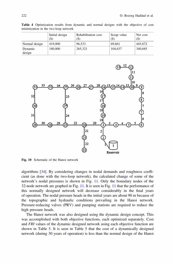
algorithms [34]. By considering changes in nodal demands and roughness coeffi-cient (as done with the two-loop network), the calculated change of some of thenetwork’s nodal pressures is shown in Fig. 11. Only the boundary nodes of the32-node network are graphed in Fig. 11. It is seen in Fig. 11 that the performance ofthis normally designed network will decrease considerably in the final yearsof operation. The nodal pressure heads in the initial years are about 90 m because ofthe topographic and hydraulic conditions prevailing in the Hanoi network.Pressure-reducing valves (PRV) and pumping stations are required to reduce thehigh pressure heads.

The Hanoi network was also designed using the dynamic design concept. Thiswas accomplished with both objective functions, each optimized separately. Costand FRI values of the dynamic designed network using each objective function areshown in Table 5. It is seen in Table 5 that the cost of a dynamically designednetwork (during 30 years of operation) is less than the normal design of the Hanoi

Table 4 Optimization results from dynamic and normal designs with the objective of costminimization in the two-loop network

Initial design($)

Rehabilitation cost($)

Scrap value($)

Net cost($)

Normal design 419,000 96,533 69,661 445,872

Dynamicdesign

180,000 265,321 104,637 340,685

Fig. 10 Schematic of the Hanoi network

222 O. Bozorg Haddad et al.

network. On the other hand, by designing the network using the FRI objectivefunction, a reliability index value was obtained equal to 1.36 with a cost equal to$10,670,531.

Figure 12 depicts envelope curves of the nodal pressures of the dynamicallydesigned Hanoi network optimizing each objective function separately. By com-paring Fig. 12 with Fig. 11, it is noticeable that the nodal pressures of the network

-80

-30

20

70

120

0 5 10 15 20 25 30

Pre

ssur

e he

ad (

m)

Time (year)

Node 2 Node 3Node 18 Node 19Node 20 Node 21Node 28 Minimum required

Fig. 11 Changes of nodal pressure heads in Hanoi network from normal design withoutrehabilitation during operational period

Table 5 Cost and FRI valuesfrom the dynamicallydesigned Hanoi networkoptimizing each objectivefunction separately

Objective function Cost ($) FRI

FRI maximization 10,670,531 1.36

Cost minimization 4,910,814 0.40

0

20

40

60

80

100

120

0 5 10 15 20 25 30

Pre

ssur

e he

ad (

m)

Time (year)

MaximumAverageMinimumMinimum requierd

0

20

40

60

80

100

120

0 5 10 15 20 25 30

Pre

ssur

e he

ad (

m)

Time (year)

MaximumAverageMinimumMinimum rerquiered

(a) (b)

Fig. 12 Envelope curve of nodal pressure in the Hanoi network from dynamic design during theoperational period, a minimizing the total network cost; b maximizing reliability

A DSS-Based Honeybee Mating Optimization (HBMO) Algorithm … 223

during its useful life are kept at an acceptable level above 30 m. It is worthmentioning that the performance of the system during the remaining years ofoperation can be improved by solving the model every few years, using new data.In this way, the model incorporates field conditions as they unfold over time.

6.3 Multi-objective Approach

The single-objective normal and dynamic designs of networks were presented andcompared for two case studies in previous sections. Yet, the nature of this problemis multi-objective because the two objectives (cost minimization and reliabilitymaximization) give rise to trade-offs between them. Therefore, using amulti-objective approach it is possible to determine those trade-offs. In this sectionthe results of multi-objective design of the two-loop and Hanoi networks are pre-sented using the multi-objective honeybee mating optimization algorithm(MOHBMO). The objectives are Eq. (2) (cost minimization) and Eq. (6) (maxi-mization of reliability). Constraints and relationships are the same assingle-objective problems. The multi-objective solutions with normal design anddynamic design can then be compared to assess their relative virtues or limitations.First, however, we compare the Pareto space of normal and dynamic designmethods.

The first step is to make an initial multi-objective optimal design of the two-loopnetwork using the two proposed objective functions. The initial design of thenetwork is performed by considering the nodal demands at the end of the WDN’sservice life (nodal demands reported by Alperovits and Shamir [3]) and the resultsare the network’s optimal pipe diameters. Ten runs of the MOHBMO algorithmwere conducted to initially design the two-loop network in which the algorithmsimultaneously attempts to optimize the objective functions of cost minimizationand FRI maximization. The results of these 10 different runs produced the Paretofrontier for this problem shown in Fig. 13. It is worth mentioning that all theanswers of this Pareto are nondominant and also feasible solutions.

The two extreme Pareto points in Fig. 13 (points A and B) were obtained usingthe single-objective design optimization models for the two-loop network, i.e.,optimizing each objective function separately. Point A represents the networkdesigned in previous sections using the cost minimization objective function andsimulated/rehabilitated during the operational period (the results of simulation andrehabilitation were shown in Figs. 6 and 7). The other extreme Pareto, point B,represents a network designed using the FRI maximization objective function.Clearly, as the reliability of the system increases, its cost increases too. The decisionmaker must choose a combination of cost and reliability found on the Paretofrontier.

In this study, the conflict resolution method proposed by Young in 1993 [79] isused to choose a point among different solutions of Pareto. According to the conflictresolution method, a desirability function is added to each objective function. By

224 O. Bozorg Haddad et al.

maximizing an equation based on the gradient of different points of the Pareto, thebest point is then chosen [79]. Using this method, point C, which is labeled by atriangle in Fig. 13, is chosen. Naming A as the solution determined by the objectivefunction of cost minimization, B as the solution achieved by FRI maximization, andC as the chosen answer using Young’s method [79], pipe diameters, network’s totalcosts, and FRI values are shown in Table 6.

Those three designs differ with respect to pipe diameters and system reliability.Therefore, their performances during the operational and rehabilitation period aredifferent from the cost and FRI reliability index viewpoints. Solution A has thelowest cost and also the worst FRI index value. As a result, this solution is expectedto need considerable rehabilitation during the operational period. In contrast, net-work B is more expensive but has better reliability than other Pareto solutions.

Fig. 13 Pareto frontier of cost and reliability index in the two-loop network corresponding to theinitial design

Table 6 Pipe diameters,network cost, and FRI forsolutions A, C, and B:two-loop network

Point Diameter (mm)

Pipe no. A C B

1 457.2 457.2 457.2

2 254.0 508.0 609.6

3 406.4 508.0 609.6

4 101.6 355.6 609.6

5 406.4 457.2 609.6

6 254.0 457.2 609.6

7 254.0 508.0 609.6

8 25.4 457.2 609.6

Cost ($) 419,000 1,090,000 3,980,000

FRI 0.02 0.97 1.2

A DSS-Based Honeybee Mating Optimization (HBMO) Algorithm … 225

Therefore, this solution B requires less rehabilitation while its total cost is higherthan the cost of other Pareto solutions. Clearly, solution C is a compromise betweencost and reliability.

The comparison of the Pareto spaces of the normal and dynamic design methodsis performed using all three benchmark solutions (A, B, and C in Table 6) asdifferent conditions for the normal design. That is, each of three solutions is sep-arately simulated during 30 years of the operational period and they are rehabili-tated if any sign of failure or underperformance appears. Results of these threenormal designs are then compared with those of the dynamic designed network.

Solutions C and B were simulated during the operational period (same assolution A in Sect. 6.1) to determine the necessity of rehabilitation for each design.The condition and changing manner of annual nodal pressures in all three solutionsshow the necessity of rehabilitation as previously shown in Fig. 6 for the least-costinitial design of the two-loop network (point A). Nodal pressures of the designpoints C and B, the same as point A, decrease considerably during the operationalyears, and, therefore, all three solutions involve rehabilitation.

Rehabilitation design for solutions C and B are performed using thesingle-objective HBMO algorithm with the two objective functions, each optimizedseparately, as was previously done for solution A. For each case, 10 different runswere conducted and the best results are considered. The normal design (initiallydesigned and then rehabilitated) of all three networks was performed using bothobjective functions. Table 7 presents a comparison of results of the normal (solu-tions A, C, and B) and dynamic designs of the two-loop network (the dynamicdesigns were described in Sect. 2), using the minimum cost objective function. It isnow possible to compare the Pareto space of the normal design with that of thedynamic design.

Figure 14 shows results of the optimization problem of the two-loop networkdesign for normal (solutions A, C, and B) and dynamic designs. Each pair of pointsshown in Fig. 14 is relevant to the single-objective normal/dynamic design of thetwo-loop network optimizing each objective function separately.

Table 7 Optimization results of normal (solutions A, C, and B) and dynamic designs showing thevalues of the two objective functions

Designtype

Initial cost ofnetworkinstallation inyear zero ($)

Rehabilitationcost ($)

Residualvalue ($)

Net cost of networkinstallation andrehabilitation (Normaldesign) or dynamic design($)

B 3,980,000 278,522 1,424,801 2,833,721

C 1,090,000 144,918 315,934 918,984

A 419,000 96,533 69,661 445,872

Dynamicdesign

180,000 265,321 104,637 340,685

226 O. Bozorg Haddad et al.

It is seen in Fig. 14 that the dynamic design was able to improve the cost andFRI in comparison with the normal design (solutions A, B, and C). In other words, asingle-objective design of the two-loop network to minimize the network’s costusing the dynamic design method yielded the least cost in comparison with solu-tions A, C, and B. Similarly, dynamic design reached a considerably better fuzzyreliability index (FRI) than normal designs. Figure 14 indicates that if the two-loopnetwork is designed in a multi-objective manner, the Pareto set obtained from thedynamic design method will dominate other Pareto sets yielded by normal designs.In other words, the Pareto frontier from the dynamic design will dominate all otherpoints existing on other Paretos.

The comparison presented in Fig. 14 also shows the influence of the initialdesign on the design of rehabilitation period. It is seen in Fig. 14 that the normallydesigned network is worse than the dynamic design judged by economics andhydraulic reliability, in all three initially designed networks using cost minimization(solution A), FRI maximization (solution B), and trade-off between these twoobjectives (solution C). As a result, it is concluded that economic and hydraulicconditions of the network during its total useful life will definitely improve if thenetwork is initially designed by considering rehabilitation during its service life.

The third prominent feature observed in Fig. 14 is the comparison between thebroadness of the dynamic and normal-design Paretos. Figure 14 establishes that thedynamic design Pareto is broader than the Paretos obtained from normal designs.That is, the dynamic design provides a wider range of solutions to decision makers.The close proximity of normal-design Pareto solutions (pair of nodes for solutionsA, C, and B) in comparison with dynamic design, renders the multi-objectivedesign of networks A, C, and B meaningless. Thus, in this study the MOHBMOalgorithm is useful for the multi-objective dynamic design of the two-loop network,only.

0

1

2

3

4

5

6

0 2 4 6

Cos

t (×

10 $

)

FRI

Dynamic design AC B

6

Fig. 14 Results of the single-objective optimization problem in the two-loop network design fromnormal and dynamic designs

A DSS-Based Honeybee Mating Optimization (HBMO) Algorithm … 227

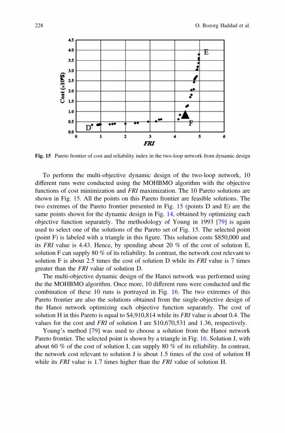
To perform the multi-objective dynamic design of the two-loop network, 10different runs were conducted using the MOHBMO algorithm with the objectivefunctions of cost minimization and FRI maximization. The 10 Pareto solutions areshown in Fig. 15. All the points on this Pareto frontier are feasible solutions. Thetwo extremes of the Pareto frontier presented in Fig. 15 (points D and E) are thesame points shown for the dynamic design in Fig. 14, obtained by optimizing eachobjective function separately. The methodology of Young in 1993 [79] is againused to select one of the solutions of the Pareto set of Fig. 15. The selected point(point F) is labeled with a triangle in this figure. This solution costs $850,000 andits FRI value is 4.43. Hence, by spending about 20 % of the cost of solution E,solution F can supply 80 % of its reliability. In contrast, the network cost relevant tosolution F is about 2.5 times the cost of solution D while its FRI value is 7 timesgreater than the FRI value of solution D.

The multi-objective dynamic design of the Hanoi network was performed usingthe the MOHBMO algorithm. Once more, 10 different runs were conducted and thecombination of these 10 runs is portrayed in Fig. 16. The two extremes of thisPareto frontier are also the solutions obtained from the single-objective design ofthe Hanoi network optimizing each objective function separately. The cost ofsolution H in this Pareto is equal to $4,910,814 while its FRI value is about 0.4. Thevalues for the cost and FRI of solution I are $10,670,531 and 1.36, respectively.

Young’s method [79] was used to choose a solution from the Hanoi networkPareto frontier. The selected point is shown by a triangle in Fig. 16. Solution J, withabout 60 % of the cost of solution I, can supply 80 % of its reliability. In contrast,the network cost relevant to solution J is about 1.5 times of the cost of solution Hwhile its FRI value is 1.7 times higher than the FRI value of solution H.

Fig. 15 Pareto frontier of cost and reliability index in the two-loop network from dynamic design

228 O. Bozorg Haddad et al.

7 Conclusion

This chapter presented a DSS for the long-term design and operation of waterdistribution networks demonstrating the importance and usefulness of the simul-taneous optimization of initial design and rehabilitation of WDNs. Changes in anetwork’s condition during its operational period were simulated and initiallyintroduced to the DSS using equations suggested in previous studies. The simul-taneous initial and rehabilitation design of two case studies was performed as themain DSS planning strategy by proposing a method named dynamic design ofWDNs. The WDN optimization problem was posed as a single- and multi-objectiveoptimization problem with minimum cost and maximum fuzzy reliability index astwo separate objectives. The HBMO and MOHBMO algorithms were used as theoptimization tools for solving this discrete, nonlinear, complex, and large-scaledesign and operation problem. Although an all-encompassing, quantitative DSS isyet to be developed, the approach described in this chapter takes into account thestructural and hydraulic state of the network while providing a framework for thefuture inclusion of other considerations as well. Results indicated that the dynamicdesign method is able to decrease the total capital cost of the WDN installation andrehabilitation while it can improve the performance of the system from the view-point of reliability. The simultaneous initial and rehabilitation designs of the net-work made it possible to postpone the installation cost by considering the network’scondition in future years, leading to considerable savings in the project.Additionally, multi-objective dynamic design of networks produces larger solutionspaces than single-objective optimization.

The DSS based on the dynamic design method encompasses three separate fieldsof WDN studies, namely, initial network design, rehabilitation activities, and pre-diction of different operational period tasks such as hydraulic conditions or

Fig. 16 Pareto frontier of cost and reliability index for the Hanoi network from dynamic design

A DSS-Based Honeybee Mating Optimization (HBMO) Algorithm … 229

water-demand volumes. Each of these research fields is being separately studied byinvestigators around the world. The dynamic design method is likely to evolve asnew findings emerge from new research.

References

1. Afshar, A., Bozorg Haddad, O., Marino, M.A., Adams, B.J.: Honey-bee mating optimization(HBMO) algorithm for optimal reservoir operation. J. Franklin Inst. 344(5), 452–462 (2007)

2. Afshar, A., Shafii, M., Bozorg Haddad, O.: Optimizing multi-reservoir operation rules: animproved HBMO approach. J. Hydroinformatics 13(1), 121–139 (2010)

3. Alperovits, E., Shamir, U.: Design of optimal water distribution systems. Water Resour. Res.13(6), 885–900 (1977)

4. Alvisi, S., Franchini, M.: Multiobjective optimization of rehabilitation and leakage detectionscheduling in water distribution systems. J. Water Res. Plann. Manage. 135(6), 426–439(2009)

5. Arulraj, G.P., Suresh, H.R.: Concept of significance index for maintenance and design of pipenetworks. J. Hydraul. Eng. (ASCE) 121(11), 833–837 (1995)

6. Berardi, L., Kapelan, Z., Giustolisi, O., Savic, D.A.: Development of pipe deteriorationmodels for water distribution systems using EPR. J. Hydroinformatics 10(2), 113–126 (2008)

7. Bozorg Haddad, O., Marino, M.A.: Dynamic penalty function as a strategy in solving waterresources combinatorial optimization problems with honey-bee optimization (HBMO)algorithm. J. Hydroinformatics 9(3), 233–250 (2007)

8. Bozorg Haddad, O., Mariño, M.A.: Optimum operation of wells in coastal aquifers. Proc. Inst.Civil Eng. Water Manage. 164(3), 135–146 (2011)

9. Bozorg Haddad, O., Afshar, A., Mariño, M.A.: Honey-bees mating optimization (HBMO)algorithm: a new heuristic approach for water resources optimization. Water Resour. Manage.20(5), 661–680 (2006)

10. Bozorg Haddad, O., Adams, B.J., Mariño, M.A.: Optimum rehabilitation strategy of waterdistribution systems using the HBMO algorithm. J. Water Supply Res. Technol. 151, 337–350(2008)

11. Bozorg Haddad, O., Afshar, A., Marino, M.A.: Honey-bee mating optimization (HBMO)algorithm in deriving optimal operation rules for reservoirs. J. Hydroinformatics 10(3), 257–264 (2008)

12. Bozorg Haddad, O., Afshar, A., Marino, M.A.: Design-operation of multi-hydropowerreservoirs: HBMO approach. Water Resour. Manage. 22(12), 1709–1722 (2008)

13. Bozorg Haddad, O., Afshar, A., Marino, M.A.: Optimization of non-convex water resourceproblems by honey-bee mating optimization (HBMO) algorithm. Eng. Comput. (Swansea,Wales), 26(3), 267–280 (2009)

14. Bozorg Haddad, O., Moradi-Jalal, M., Mirmomeni, M., Kholghi, M.K.H., Mariño, M.A.:Optimal cultivation rules in multi-crop irrigation areas. Irr. Drain. 58(1), 38–49 (2009)

15. Bozorg Haddad, O., Mirmomeni, M., Mariño, M.A.: Optimal design of stepped spillwaysusing the HBMO algorithm. Civil Eng. Environ. Syst. 27(1), 81–94 (2010)

16. Bozorg Haddad, O., Mirmomeni, M., ZarezadehMehrizi, M., Mariño, M.A.: Finding theshortest path with honey-bee mating optimization algorithm in project management problemswith constrained/unconstrained resources. Comput. Optim. Appl. 47(1), 97–128 (2010)

17. Bozorg Haddad, O., Moradi-Jalal, M., Mariño, M.A.: Design-operation optimisation ofrun-of-river power plants. Proc. Inst. Civil Eng. Water Manage. 164(9), 463–475 (2011)

18. Clark, R.M., Stafford, C.L., Goodrich, J.A.: Water distribution systems: a spatial and costevaluation. J. Water Resour. Plann. Manage. (ASCE) 108, 243–256 (1982)

230 O. Bozorg Haddad et al.

19. Cunha, M.C., Sousa, J.: Hydraulic infrastructures design using simulated annealing.J. Infrastruct. Syst. (ASCE) 7(1), 32–39 (2001)

20. Cunha, M.C., Sousa, J.: Water distribution network design optimization: simulated annealingapproach. J. Water Resour. Plann. Manage. (ASCE) 125(4), 215–221 (1999)

21. Dandy, G.C., Engelhardt, M.: Multi-objective trade-offs between cost and reliability in thereplacement of water mains. J. Water Resour. Plann. Manage. ASCE 132(2), 79–88 (2006)

22. Elstad, J.C., Byer, P.H., Adams, B.J.: Optimal timing of the restoration of watermain carryingcapacity. In: Proceedings of the CSCE Centennial Conference, Montreal, P.Q., pp. 60–70(1987)

23. Engelhardt, M.O., Skipworth, P.J., Savic, D.A., Saul, A.J., Walters, G.A.: Rehabilitationstrategies for water distribution networks: a literature review with a UK perspective. UrbanWater 2, 153–170 (2000)

24. Eusuff, M.M., Lansey, K.E.: Optimization of water distribution network design using theshuffled frog leaping algorithm. J. Water Resour. Plann. Manage. (ASCE) 129(3), 210–225(2003)

25. Fallah-Mehdipour, E., Bozorg Haddad, O., Beygi, S., Mariño, M.A.: Effect of utility functioncurvature of Young’s bargaining method on the design of WDNs. Water Resour. Manage. 25(9), 2197–2218 (2011)

26. Fallah-Mehdipour, E., Bozorg Haddad, O., Mariño, M.A.: MOPSO algorithm and itsapplication in multipurpose multireservoir operations. J. Hydroinformatics 13(4), 794–811(2011)

27. Fallah-Mehdipour, E., Bozorg Haddad, O., Mariño, M.A.: Real-time operation of reservoirsystem by genetic programming. Water Resour. Manage. 26(14), 4091–4103 (2012)

28. Fallah-Mehdipour, E., Bozorg Haddad, O., RezapourTabari, M.M., Mariño, M.A.: Extractionof decision alternatives in construction management projects: application and adaptation ofNSGA-II and MOPSO. Expert Syst. Appl. 39(3), 2794–2803 (2012)

29. Fallah-Mehdipour, E., Bozorg Haddad, O., Mariño, M.A.: Developing reservoir operationaldecision rule by genetic programming. J. Hydroinformatics 15(1), 103–119 (2013)

30. Fallah-Mehdipour, E., Bozorg Haddad, O., Mariño, M.A.: Extraction of multicrop planningrules in a reservoir system: Application of evolutionary algorithms. J. Irri. Drain. Eng. 139(6),490–498 (2013)

31. Fujiwara, O., Kang, D.B.: A two-phase decomposition method for optimal design of loopedwater distribution networks. Water Resour. Res. 26(4), 539–549 (1990)

32. Geem, Z.W.: Optimal cost design of water distribution networks using harmony search.J. Eng. Optim. 38(3), 259–280 (2005)

33. Ghajarnia, N.: Multi-objective dynamic design of water distribution networks. M.Sc. thesis,Department of Irrigation and Reclamation Engineering, University of Tehran, Iran (2009)

34. Ghajarnia, N., Bozorg Haddad, O., Mariño, M.A.: Performance of a novel hybrid algorithm inthe design of water networks. Water Manage. 164(4), 173–191 (2011)

35. Goulter, I.C., Bouchart, F.: Reliability constrained pipe networks model. J. Hydraul. Eng.(ASCE) 16(2), 221–229 (1990)

36. Goulter, I.C., Lussier, B.M., Morgan, D.R.: Implications of head loss path choice in theoptimization of water distribution networks. Water Resour. Res. 22(5), 819–822 (1986)

37. Halhal, D., Walters, G.A., Savic, D.A., Ouazar, D.: Scheduling of water distribution systemrehabilitation using structured messy genetic algorithms. Evol. Comput. 7(3), 311–329 (1999)

38. Jahanshahi, G., Bozorg Haddad, O.: Honey-bee mating optimization (HBMO) algorithm foroptimal design of water distribution systems. World Environmental and Water ResourcesCongress, Honolulu, Hawaii, United States, 12–16 May 2008

39. Kanakoudis, V.K.: A troubleshooting manual for handling operational problems in water pipenetworks. Water Supply Res. Technol. AQUA IWAp 53(2), 109–124 (2004)

40. Kanakoudis, V.K.: Vulnerability based management of water resources systems.Hydroinformatics WAp 6(2), 133–156 (2004)

41. Kanakoudis, V.K., Tolikas, D.K.: The role of leaks and breaks in water networks—technicaland economical solutions. Water Supply Res. Technol. AQUA IWAp 50(5), 301–311 (2001)

A DSS-Based Honeybee Mating Optimization (HBMO) Algorithm … 231

42. Kanakoudis, V.K., Tolikas, D.K.: Assessing the Performance Level of a water system. WaterAir Soil Pollut. 4–5, 307–318 (2004)

43. Karimi-Hosseini, A., Bozorg Haddad, O., Mariño, M.A.: Site selection of raingauges usingentropy methodologies. Proc. Instit. Civil Eng. Water Manage. 164(7), 321–333 (2011)

44. Keen, P.G.W., Morton, M.S.S.: Decision Support Systems: An Organizational Perspective.Addison-Wesley Pub (1978)

45. Kessler, A., Shamir, U.: Analysis of the linear programming gradient method for optimaldesign of water supply networks. Water Resour. Res. 25(7), 1469–1480 (1989)

46. Kim, J.H., Mays, L.W.: Optimal rehabilitation model for water-distribution systems. J. WaterRes. Plann. Manage. (ASCE) 120(5), 674–692 (1994)

47. Kleiner, Y., Adams, B.J., Rogers, J.S.: Long-term planning methodology for water distributionsystem rehabilitation. Water Resour. Res. 34(8), 2039–2051 (1998)

48. Kleiner, Y., Adams, B.J., Rogers, J.S.: Selection and scheduling of rehabilitation alternativesfor water distribution systems. Water Resour. Res. 34(8), 2053–2061 (1998)

49. Lansey, K.E., Basnet, C., Mays, L.W., Woodburn, J.: Optimal maintenance scheduling forwater distribution systems. Civil Eng. Syst. 9(3), 211–226 (1992)

50. Lippai, I., Heaney, J.P., Laguna, M.: Robust water system design with commercial intelligentsearch optimizers. J. Comput. Civil Eng. 13(3), 135–143 (1999)

51. Maier, H.R., Simpson, A.R., Zencchin, A.C., Foong, W.K., Phang, K.Y., Seah, H.Y., Tan, C.L.: Ant colony optimization for design of water distribution systems. J. Water Resour. Plann.Manage. 129(3), 200–209 (2003)

52. Male, J.W., Walski, T.M., Slutski, A.H.: Analyzing watermain replacement policies. J. WaterResour. Plann. Manage. (ASCE) 116(3), 363–374 (1990)

53. Nafi, A., Kleiner, Y.: Scheduling renewal of water pipes while considering adjacency ofinfrastructure works and economies of scale. J. Resour. Plann. Manage. (ASCE) 136(5), 519–530 (2010)

54. Nafi, A., Werey, C., Llerena, P.: Water pipe renewal using a multi-objective optimizationapproach. Can. J. Civ. Eng. 35, 87–94 (2008)

55. Orouji, H., Bozorg Haddad, O., Fallah-Mehdipour, E., Mariño, M.A.: Estimation ofMuskingum parameter by meta-heuristic algorithms. Proc. Inst. Civil Eng Water Manage.166(6), 315–324 (2013)

56. Prasad, T.D., Park, N.S.: Multiobjective genetic algorithms for design of water distributionnetworks. J. Water Resour. Plann. Manage. (ASCE) 130(1), 73–82 (2004)

57. Quindry, G.E., Brill, E.D., Liebman, J.C.: Optimization of looped water distribution systems.J. Environ. Eng. 107(4), 665–679 (1981)

58. Roshani, E., Filion, Y.R.: Event based network rehabilitation planning and asset management.In: 14th annual Water Distribution Systems Analysis Conference (WDSA), Adelaide,Australia, pp. 933–943 (2012)

59. Rossman, L.A.: EPANET user manual. Drinking Water Research Division, Risk ReductionEngineering Laboratory, Office of Research and Development, U.S. Environmental ProtectionAgency, Cincinnati, OH, July 2000

60. Sabbaghpour, S., Naghashzadehgan, M., Javaherdeh, K., Bozorg Haddad, O.: HBMOalgorithm for calibrating water distribution network of Langarud city. Water Sci. Technol. 65(9), 1564–1569 (2012)

61. Savic, D.A., Walters, G.A.: Genetic algorithms for least-cost design of water distributionnetworks. J. Water Resour. Plann. Manage. (ASCE) 123(2), 67–77 (1997)

62. Schneiter, C.R., Haims, Y.Y., Li, D., Lambert, J.H.: Capacity reliability of water distributionnetworks and optimum rehabilitation decision making. Water Resour. Res. 32(7), 2271–2278(1996)

63. Seifollahi-Aghmiuni, S., Bozorg Haddad, O., Omid, M.H., Mariño, M.A.: Long-termefficiency of water networks with demand uncertainty. Proc. Inst. Civil Eng. Water Manage.164(3), 147–159 (2011)

232 O. Bozorg Haddad et al.

64. Seifollahi-Aghmiuni, S., Bozorg Haddad, O., Omid, M.H., Mariño, M.A.: Effects of piperoughness uncertainty on water distribution network performance during its operationalperiod. Water Resour. Manage 27(5), 1581–1599 (2013)

65. Shamir, U., Howard, C.D.D.: An analytic approach to scheduling pipe replacement. J. Am.Water Works Assoc. 71(5), 248–258 (1979)

66. Sharp, W.W., Walski, T.M.: Predicting internal roughness in water mains. J. Am. WaterWorks Assoc. 80, 34–40 (1988)

67. Shokri, A., Bozorg Haddad, O., Mariño, M.A.: Algorithm for increasing the speed ofevolutionary optimization and its accuracy in multi-objective problems. Water Resour.Manage. 27(7), 2231–2249 (2013)

68. Sol, H.G., Takkenberg C.A.Th., De VriesRobbe, P.F.: Expert systems and artificialintelligence in decision support systems. In: Proceedings of the Second MiniEuroconference, Springer, Lunteren, The Netherlands, 17–20 Nov 1985 (1987)

69. Solgi, M., Bozorg Haddad, O., Seifollahi-Aghmiuni, S., Loaiciga, H.A.: Intermittent operationof water distribution networks considering equanimity and justice principles. J. Pipeline Syst.Eng. Pract. (2015). doi:10.1061/(ASCE)PS.1949-1204.0000198

70. Soltanjalili, M., Bozorg Haddad, O., Mariño, M.A.: Operating water distribution networksduring water shortage conditions using hedging and intermittent water supply concepts.J. Water Resour. Plann. Manage. (2013) In Press

71. Soltanjalili, M., Bozorg Haddad, O., Seifollahi-Aghmiuni, S., Mariño, M.A.: Waterdistribution networks simulation by optimization approaches. Water Sci. Technol. WaterSupply (2013) In Press

72. Su, Y.C., Mays, L.W.: New methodology for determining the optimal rehabilitation andreplacement of water distribution system components. In: Abt S.R., Gessler J. (eds.)Proceedings of Hydraulic Engineering ASCE National Conference, Edited by , (ASCE), NewYork, N.Y., 1149–1154 (1988)

73. Suribabu, C.R., Neelakantan, T.R.: Design of water distribution networks using particle swarmoptimization. J. Urban Water 3(2), 111–120 (2006)

74. Todini, E.: Looped water distribution networks design using a resilience index based heuristicapproach. J. Urban Water 2(3), 115–122 (2000)

75. Tsitsifli, S., Kanakoudis, V., Bakouros, L.: Pipe networks risk assessment based on survivalanalysis. Water Resour. Manage. 2514, 3729–3746 (2011)

76. Walski, T.M.: The wrong paradigm-Why water distribution optimization doesn’t work.J. Water Resour. Plann. Manage. (ASCE) 127(4), 203–205 (2001)

77. Walski, T.M., Pelliccia, A.: Economic analysis of watermain breaks. J. Am. Water WorksAssoc. 74(3), 140–147 (1982)

78. Walski, T.M.: Optimization and pipe-sizing decisions. J. Water Resour. Plann. Manage.(ASCE) 121(4), 340–343 (1995)

79. Young, H.P.: An evolutionary model of bargaining. J. Econ. Theory 59, 145–168 (1993)

A DSS-Based Honeybee Mating Optimization (HBMO) Algorithm … 233

Application of the Simulated AnnealingAlgorithm for Transport InfrastructurePlanning

Ana Laura Costa, Maria Conceição Cunha, Paulo A.L.F. Coelhoand Herbert H. Einstein

Abstract Decisions in planning for transport infrastructure are the result of com-plex technical, political, and societal concerns. Its context of limited public fundingand large costs require that decision making is soundly supported. When addressingreal-world problems, however, it is extremely difficult to ascertain the systemconfiguration yielding the most value. Different alternatives exist that trade-offinterrelated factors governing the value of the configurations. Metaheuristics can beof assistance when solving such real-world problems. This chapter presents anapplication of the simulated annealing algorithm to solve an integrated approach tohigh-speed rail planning. The algorithm capabilities in addressing the intricaciesimposed by large and complex problems are discussed.

Keywords Metaheuristics � Simulated annealing � Optimization � Parameter cal-ibration � High-speed rail modeling

A.L. Costa � M.C. Cunha (&) � P.A.L.F. CoelhoDepartment of Civil Engineering, University of Coimbra, Coimbra, Portugale-mail: mccunha@dec.uc.pt

A.L. Costae-mail: alcosta@dec.uc.pt

P.A.L.F. Coelhoe-mail: pac@dec.uc.pt

H.H. EinsteinDepartment of Civil and Environmental Engineering,Massachusetts Institute of Technology, Cambridge, USAe-mail: einstein@mit.edu

© Springer International Publishing Switzerland 2016X.-S. Yang et al. (eds.), Metaheuristics and Optimization in Civil Engineering,Modeling and Optimization in Science and Technologies 7,DOI 10.1007/978-3-319-26245-1_11

235

1 Introduction

1.1 Planning for Transport Infrastructure

Building and operating large transport infrastructure is expensive. Significantinvestments are necessary and have to compete for the allocation of limited gov-ernment resources. The context of public funding drives an increased demand foraddressing key social, economic, and environmental concerns. In the case of roadand railway infrastructure, the planning stage considers the appraisal of multipleinfrastructure configurations and technical solutions. Interrelations between localcharacteristics and the infrastructure specifics can be established for determining theproject solutions yielding the most value. Studying different alternatives is ofparamount importance as the subsequent project design stage further details thecharacteristics of the infrastructure within boundaries imposed by planning.

1.1.1 The Case of High-Speed Rail: Definition of Stations

Ridership and demand capture from other modes are decisive for HSR projects.Amongst others, they are affected by the location of the HSR stations defining theconnections established by the system [1]. In addition to journey-related factorssuch as connection time or comfort, other elements affect the decision to travel byHSR. Accessibility to HSR stations is a major factor influencing the choice of railinstead of other modes [1–3] and increasing the number of stations within the HSRsystem increases accessibility. On the other hand, a rising number of intermediatestations increase journey times for passengers, decreasing the attractiveness of theHSR and having a negative impact on ridership [1, 4].

These counteracting effects for the definition of which cities to connect need tobe addressed at the planning stage [5], along with the political decisions thatultimately enable the HSR project [6].

1.1.2 The Case of High-Speed Rail: Layout and Technical Solutions

The connection between HSR stations is established by trains circulating, as thedesignation suggests, at significantly higher speeds than those operated in con-ventional railways. Upgraded existing lines support speeds of circa 200 km/h whilespecially built lines are generally equipped for speeds in excess of 250 km/h [7].

The high operating speeds require that the HSR infrastructure complies withstrict layout specifics, particularly for the radii of horizontal curves and the longi-tudinal gradient of linear sections. Large centrifugal acceleration imposed on trains,as a result of high speeds and small radii of horizontal curves, compromises thequality of the service and, in extreme cases, safety. It can also increase trackdegradation and reduce the components lifetime. The radii of horizontal curves

236 A.L. Costa et al.

should be as large as possible: standards define comfort values that can beexceptionally reduced due to project difficulties until an absolute minimum radiiimposed by safety concerns [8]. Conversely, smaller longitudinal gradients desir-able and absolute maximum gradients are established [7]. It is advantageous,however, to implement minimum gradients that facilitate drainage. Steeper slopesresult in increased energy consumption and braking distances for downward trainsthat may reduce the line capacity, particularly for freight and passenger-mixedtraffic lines.

In addition to the strict requirements imposed on the HSR layout, further diffi-culties are imposed by the deployment site. Large variations of ground elevations,irregular land-use patterns, heterogeneous and hazardous geotechnical conditions,and population density are common challenges to HSR projects. These are over-come by technical solutions including embankments, cuts, retaining walls, bridges,and tunnels. In each case, however, strict displacement limits of the HSR tracksneed to be assured [9] through adequate correspondence between the technicalsolution and the deployment site characteristics. The multiple layout possibilitiesfor connecting any two HSR stations coupled with the interrelations betweeninfrastructure and local characteristics make the HSR planning process a complexone.

1.1.3 The Case of High-Speed Rail: Cost Overview

A comprehensive model to estimate the overall costs of intercity transportationsystems is proposed by Levinson et al. [10] considering social costs in addition toconstruction, operation, and maintenance costs. Applications to HSR by Levinsonet al. in 1997 [11] suggest the HSR fares well in social costs, including pollution,accidents, and noise compared with air travel and highways. Nonetheless, protestsagainst HSR configuration have occurred [12]. In Europe, United States, and Chinathe concerns stated include alteration of landscapes and proximity to schools, issuesfor which alternative solutions can be studied at the planning stage.

Conversely, the large HSR infrastructure capital cost is the main disadvantagecompared to air travel and highway systems. Such costs, however, can vary greatly.Based on data from worldwide HSR projects, Campos and de Rus in 2009 [12]observe HSR construction costs ranging from €4.7 million to €65.8 million (2005)per km. These large variations relate to intrinsic characteristics of the projects.Topographic characteristics, HSR layout, and technical solutions and the type oftraffic explain major differences within Europe [12]. Compare the adoption of largerlongitudinal gradients in France’s HSR passenger dedicated line, avoiding theexpensive major tunnel and viaduct construction, with Germany’s ICE mixed trafficand stricter layout restrictions coupled with corridors over mountainous terrains [5].

Application of the Simulated Annealing Algorithm … 237

1.1.4 Complexity for High-Speed Rail Decision Making

In general, the higher the operating speed is the stricter the design requirements are,resulting in large construction and maintenance costs of an HSR system. Whilelarge expenditures are required, the HSR has advantages over other transportationmodes and the decisions at the planning stage, varying the intermediate citiesconnected, the corridors, and the technical solutions have an important influence onthe resulting costs and HSR performance.

Multiple alternatives can be studied that trade-off interrelated factors governingthe value of the HSR solutions. This can hardly be achieved without the support ofcomprehensive tools capable of integrated approaches that systematically addressthe complexities involved in decision making.

1.2 Optimization of Linear Transport Infrastructure

Mathematical optimization models are widely used in engineering for addressinglarge and complex problems. An objective function expresses the measure of wealthto be optimized by changing design variables and subject to constraints that definethe feasibility of the solutions. However complex the formulated models may be,these are nonetheless representations of reality. The ability to express the realproblems depends on the simplifications assumed, in this case the representation ofthe linear transport infrastructure problem. Once a satisfactory formulation isestablished for the problem, it is necessary to solve the optimization model and findthe solution yielding the most value. Multiple solving techniques exist and, amongothers, the choice should take into consideration the ability to deal with the modelspecifics.

1.2.1 Representation of Problem Specifics

Several models have been developed for the optimization of linear transportinfrastructure, particularly for highway alignment optimization in detailed stages ofthe problem.

Jong et al. in 1998 [13] propose a model for the optimization of horizontal andthree-dimensional highway alignments considering the minimization of construc-tion costs, user costs, and location-dependent costs subject to restrictions of thehighway geometry layout and location. Geographic Information Systems(GIS) integration is not considered [13] and difficulties exist in representing loca-tion cost items. An important concern when modeling linear transport infrastructureis the interrelation of the infrastructure characteristics and the site conditions thatare subject to irregular patterns and large variations. GIS integration is developedby Jong et al. in 2000 [14] for optimization of horizontal alignments. However, byoptimizing horizontal alignments only, limitations are imposed for the highway

238 A.L. Costa et al.

construction cost formulations as these depend on the highway elevation relativelyto the ground. Other approaches have been developed that focus on modeling theoptional connection of intermediate locations and infrastructure specifics [15, 16],environmental concerns [17, 18], or cost formulations [19–21].

At the smaller planning scale Gipps et al. in 2001 [22] develop a comprehensiveframework for the optimization of linear transport infrastructures. It considers theinfluence of variable geotechnical behavior influencing the technical solutions andtheir construction and maintenance costs. This is an important factor for realisticallyassessing construction costs that is not considered in the preceding examples. Gippset al. in 2001 [22], however, do not integrate the connection of intermediatelocations and the infrastructure alignment definition, which are two intertwinedissues, particularly for HSR planning [4].

The examples presented are not exhaustive but demonstrate limitations andcapabilities of existing models. It is shown that the consideration of an integratedthree-dimensional approach including discontinuous cost items is required forrealistically modeling the problem. The lack of a comprehensive cost formulationleads to suboptimal solutions. However, when considering comprehensive costformulations for the optimization of linear transport infrastructure, the cost functionbecomes an implicit function of the decision variables, resulting innon-differentiable and noisy cost functions [23]. These complexities need to beaddressed by the solving techniques.

1.2.2 Solving Techniques

Various solving techniques have been considered. Parker in 1977 [24] proposed amethod for solving highway corridor optimization combining linear programmingand shortest path algorithms. The linearity requirements allow only for a limited set ofproblem costs and constraints to be considered and difficulties exist in dealing withbackward bending alignments. The latter limitation has also been observed in solvingalignment optimization problems with dynamic programming [25]. However, chal-lenging land-use patterns or topographic conditions may impose infrastructure con-figurations that significantly deviate from the direct straight path between two points.Studies by Chew et al. in 1989 [26] used gradient-based search methods to solvehighway alignment optimization problem. The need to assess cost gradients haslimitations in addressing discontinuous cost functions that are needed to realisticallyformulate the problem. Kang et al. in 2012 [27] further discuss this, observing lim-itations in various search methods other than metaheuristics for addressing thecomplexity of optimization models that realistically represent the problem.

Metaheuristics including particle swarm, genetic algorithms, and simulatedannealing [14, 27–30] have been successfully applied to linear transport infras-tructure optimization problems. Among other characteristics, flexibility is providedby metaheuristics for taking into account the specifics of real cases. In this chapter,an application of the simulated annealing algorithm is discussed for solving athree-dimensional approach to high-speed rail planning optimization.

Application of the Simulated Annealing Algorithm … 239

2 The Simulated Annealing Algorithm

2.1 Overview

The simulated annealing algorithm is inspired by the annealing process of materialsfrom high energy states into low energy states used extensively in the steel andglass industries. In this process, the material is initially heated until reaching a highenough temperature that allows the particles to move. Slow and controlled coolingfollows that then allows the particles to rearrange into configurations correspondingto very low energy states. Lower temperatures represent lower energy states butslow cooling is necessary to avoid obtaining suboptimal configurations. Thisconcept is expressed by the Metropolis algorithm [31] that has been generalized byKirkpatrick et al. in 1983 [32] to solve the travelling salesman problem. Theapplications by Kirkpatrick et al. in 1983 [32] and later Cerny in 1985 [33] to solvethe travelling salesman problem draw an analogy between obtaining the lowestenergy configuration of a system and achieving the global optimum solution for theoptimization problem [34]. In the analogy, the solutions to the optimization prob-lem correspond to the configurations of a physical system and the objective functionvalue of a solution corresponds to the energy of a configuration.

According to the Metropolis algorithm, if a current system configuration i ofenergy Ei is rearranged into a configuration j of energy Ej, the probability p thatj will be the new current system configuration in a minimization problem is givenby Eq. (1).

p ¼ min ½1; exp ð� Ej � Ei� �

=ðkBtÞÞ� ð1Þ

where kB is the Boltzman’s constant and t is the temperature.Apart from the physical analogy, the simulated annealing algorithm can be

regarded as a stochastic technique that applies a probabilistic mechanism foraccepting worsening solutions [35]. As a local search technique, the simulatedannealing algorithm considers new candidate configurations obtained by perturbinga current configuration within a neighborhood structure. This corresponds to smallchanges within the vicinity of the current configuration. Therefore, if the currentconfiguration is suboptimal but corresponds to a local optimum, it is necessary toaccept worsening configurations in order to continue the search for a global opti-mum. This is illustrated in Fig. 1.

Consider solving a minimization problem. By using the Metropolis algorithm, inaddition to accepting transitions that improve the objective function (Ej < Ei), thesimulated annealing also accepts worsening transitions (Ej > Ei). The probability ofaccepting worse solutions in Eq. (1) is given by p = exp(−(Ej − Ei)/(kBt)) anddecreases as the algorithm progresses. This acceptance rate is governed by thedecrease of a control parameter, the temperature in Eq. (1). Even if the algorithmperformance is dissociated from underlying assumptions of physical meaning,terminology borrowed from the annealing physical process is used [36].

240 A.L. Costa et al.

Aarts et al. in 1997 [34] and Dekkers and Aarts in 1991 [35] discuss how, inmathematically modeling the SAA using Markov chains, for certain conditions,asymptotic convergence to the global optimum can be proven to have probability 1.A Markov chain can be defined as a sequence of trials from a sampling process inwhich the probability of a particular trial result depends only on the previous trialresult and not on the preceding sequence according to Eq. (2) [34].

Pij kð Þ ¼ P X kð Þ ¼ j jX k � 1ð Þ ¼ if g ð2Þ

where Pij(k) is the transition probability from result i to result j at the kth trial and X(k) is a random variable defining the result of the kth trial.

Based on these principles, simulated annealing algorithms have been successfullyimplemented to solve multiple engineering problems [37]. However, Dekkers andAarts in 1991 [35] and Johnson et al. in 1989 [36] discuss that considering an infinitenumber of homogeneous Markov chains (in which the transition probability does notdepend on the trial number k) of infinite length, as required by for the asymptoticconvergence proof, is impracticable. Thus, implementations in finite time with finitelength Markov chains at a finite number of descending values of the controlparameter are required. The convergence of the algorithm is governed by a set ofparameters defining a cooling schedule that establishes how the control parameter,temperature, is decreased. These cannot guarantee global optimum convergence butits probability may increase according to the specifics of the implementation [35].

2.2 Considerations for the Algorithm Implementation

The implementation of the simulated annealing algorithm involves the definition ofan initial system configuration, the neighborhood structure and the generationprocess of new candidate configurations, and the cooling schedule. The following

SystemConfiguration (c)

ObjectiveFunction

Value(f)

c*cjci

Local Optimum f(ci )

f(cj ) > f(ci )

Global Optimumf(c*)

Fig. 1 Accepting worsening system configurations to escape local optima

Application of the Simulated Annealing Algorithm … 241

subsections discuss issues to consider when defining these elements. While thealgorithm may be applied for solving multiple problems, the best annealing algo-rithm parameters in each case depend on the problem solved and its size [36].

2.2.1 Initial System Configuration

Heuristic methods, arbitrary definition, random or best guess approaches have beenused in the literature to derive initial system configurations for implementing thesimulated annealing algorithm. It may be advantageous to start the algorithm with abetter than random configuration, particularly if it takes advantage of specificproblem structures rather than employing a general heuristic [36]. However,heuristic defined initial configurations can add overhead time to the algorithmimplementation. On the other hand, if the algorithm implementation allows thesearch of the global feasible search space of the problem, the initial system con-figuration will not limit the search nor will it influence the quality of the solutionsproduced [38]. The generation of the initial system configuration should thustrade-off overhead and running times, taking into account the problem specifics.

2.2.2 Generating New System Configurations

The generation of new candidate system configurations within a neighborhoodstructure aims at obtaining transitions that correspond to rearrangements instead ofprofound transformations. The neighborhood structure imposes boundaries to theextent of each modification of the current configuration. In addition, the degree offreedom, the number of changes at each transition, of the process influences thealgorithm performance [39]: minor changes in the configuration transitions maylimit the algorithm to explore only a limited part of the search space while theopposite profound changes may lead to a random behavior and not taking advan-tage of the neighborhood structure. The procedures to generate feasible candidateconfigurations of the system are required to address these concerns and furtheraddress difficulties that may be imposed by the problem feasibility constraints.

2.2.3 Cooling Schedule

The cooling schedule defines the evolution of the control parameter (temperature)throughout the algorithm and the number of system configurations analyzed at eachtemperature step. Two main classes of schedules exist [34, 36]: static coolingschedules and dynamic cooling schedules. Static cooling schedules implement fixedparameters which are not changed during the algorithm implementation. Dynamicschedules implement parameters governing the temperature decrease that areadapted as the algorithm progresses.

242 A.L. Costa et al.

A general approach to the cooling schedule defines criteria for initial and finalsystem temperatures, the rate with which the initial temperature is decreased untilreaching the final temperature and a minimum number of system configurations tobe evaluated at each temperature step. Figure 2 illustrates how the cooling schedulegoverns the inner loops performed within a generic implementation of the simulated

Ej< E

i

Or

Probability pj= exp (E

i – E

j)/t

n

of accepting cjis larger than

Initial Temperature t0

Initial configuration ci

with objective function value E

i

Accept cjas new

current configuration

No

Generate new candidate configurationc

i c

j

Equilibrium at tn: minimum n

1configurations reached?

End temperature criteria tf

reached?

yes

yes

No

Decrease temperaturet

n t

n+1

No

End

yes

MetropolisCriterion

Fig. 2 Flowchart of a generic implementation of the simulated annealing algorithm

Application of the Simulated Annealing Algorithm … 243

annealing algorithm. The flowchart in Fig. 2 considers a minimization problem inwhich worse solutions correspond to larger objective function values.

The initial temperature should be such that the system is considered, in analogywith the physical annealing process, “melted”. The temperature at each stepinfluences the probability of accepting configurations with worse objective functionvalues (see Metropolis criterion in Fig. 2) and thus a sufficiently large temperature,for which almost all system configurations are accepted, should be chosen initially.Kirkpatrick in 1984 [40] suggested an initial temperature that allows at least 80 %of the transitions to be accepted at the initial temperature step.

A temperature decrease occurs when equilibrium is reached at a given temper-ature step (Fig. 2). The implementation of static geometric cooling is common [36],where temperature at the n + 1 step, tn + 1 is given by tn + 1 = r. tn at a constant rate0 < r < 1. The rate with at the temperature is decreased has a substantial influenceon the quality of the solutions obtained [34, 36]. If the temperature decreases toofast, the algorithm will accept only a small number of worsening configurations andthe performance will be similar to iterative improvement, which terminates at thefirst local optimum. Conversely, if the decrease rate is too small, the algorithmperformance can resemble a random search where virtually any neighboring con-figuration is accepted.

Different cooling schedules can be implemented, including linear or logarithmiccooling [36] or more complex dynamic schedules based on the standard deviationof the objective function values of the Markov chain [35].

The equilibrium considered in the finite-time implementation of simulatedannealing relates to the number of transitions at each temperature step. A fixednumber of transitions per temperature can be established or adaptive schedules withvarying number of transitions can be implemented. The amount of time that thealgorithm spends between very high and very low temperatures affects the qualityof the solutions and adaptive cooling schedules can be tailored to such purpose [32,36].

The termination criteria establish when to stop the algorithm. It relates to thetemperature value corresponding to a “frozen” state for which no furtherimprovements of the objective function are achieved. This has been implemented inthe literature based on different criteria, including the average value of the objectivefunction [35] and a minimum number of temperature decreases below a percentagethreshold of accepted transitions [36].

3 Application for Planning Transport Infrastructure

This section discusses the implementation of the simulated annealing algorithm fora transport infrastructure planning problem. The application considers the opti-mization model proposed by Costa et al. in 2013 [30] for high-speed rail infras-tructure planning. The problem is formulated as the minimization of theinfrastructure construction costs while establishing trade-offs with possible

244 A.L. Costa et al.

infringement of the geometric design best practice values, overlay of sensitiveland-use areas, and the value of connecting intermediate cities.

Large, restrictive values represent the design best practice for the plan view ofthe infrastructure’s horizontal angles, termed normal horizontal angles. Smaller thannormal horizontal angles are admissible when difficult circumstances are encoun-tered, such as rough terrain or existing constructions in the deployment area. These,however, represent future limitations to the infrastructure operation phase thatshould be balanced with the costs of building bridges and tunnels or relocatingexisting infrastructure as required for implementing large horizontal angles (seeSect. 1.1.1). The model considers such trade-offs through penalties in the objectivefunction whenever an alignment’s horizontal angle is smaller than the normal one.An analogous approach is considered for the longitudinal gradient of the alignmentlinear sections. A penalty representing additional operation costs increases theobjective function value one aims at minimizing when gradients exceed the normalgradient value. In the case of gradients, normal values are smaller than the limitones. The negative impacts of crossing sensitive areas is also considered through apenalty in the objective function while an additional objective function term rep-resents the overall value of connecting intermediate locations.

Constraints are defined by the regulatory safety concerns of the infrastructurelayout (limit values), legislation protected land-use areas, and the obvious con-nection of the problem main cities. Several layers of spatial data are required thatare then combined with the HSR configuration for defining the construction costsand the objective function value and verify the compliance with the problemconstraints.

3.1 Implementation of the Simulated Annealing Algorithm

Implementing the simulated annealing algorithm requires that choices are maderegarding the generic cooling schedule parameters but also problem-specific issuessuch as what a system configuration is, its objective function value, the generationof new candidate configurations, and how to derive an initial configuration [36].These are here discussed for studies regarding a Portuguese high-speed railnetwork.

3.1.1 Problem-Specific Definitions

A feasible system configuration for this application is an HSR line, defined by itslinear alignments, that connects the main cities Oporto, Coimbra, and Lisbon with alllongitudinal gradients smaller than a regulatory limit, all horizontal angles (as a

Application of the Simulated Annealing Algorithm … 245

proxy for radii) larger than a regulatory limit, and that does not overlay protectedland-use areas such as natural reservations or parks. Figure 3 illustrates the datalayers used [41] and the initial system configuration for implementing the algorithm.

A neighbor of any current configuration is obtained by changing, within itsneighborhood structure, two randomly chosen nodes. Preliminary tests were per-formed considering transitions changing only one node of the HSR linear align-ment. It was observed that the SAA was not able to comprehensively canvass thesearch space of the problem when only one node was perturbed and the finalsolution depended on the initial system configuration chosen.

The initial system configuration shown in Fig. 3 was arbitrarily defined. Theregulatory limits for the geometry of the HSR layout are very strict due to the highrunning speeds of the trains. As such, randomly obtaining linear alignments con-necting Oporto, Coimbra, and Lisbon that comply with layout restrictions and

Oporto

CoimbraLisbon

Protected Land Use

Elevation

Expropriation Class

Lithology

Rivers

Fig. 3 The initial system configuration and the respective overlays with the problem spatial data[41]

246 A.L. Costa et al.

additionally none of its linear sections overlays protected land-use areas adds asignificant overhead to the computation time. Starting at an arbitrarily definedconfiguration, studies can be performed for the algorithm implementation to assessif the algorithm is able to comprehensively search the problem space, such that thefinal configuration is independent of the initial one.

The construction cost of any configuration is obtained by summing the costs ofearthworks, expropriation, bridges, and tunnels along the infrastructure length bycomparing and overlaying the HSR configuration and the local characteristics,including the influence of lithological conditions affecting the HSR cross-section[30].

3.1.2 Cooling Schedule: Equilibrium and Temperature Decrease

The studies performed show how one may define the parameters of the simulatedannealing implementation governing the decrease in the temperature, the algorithmcontrol parameter. An adaptive geometric cooling schedule is implemented basedon existing research [30, 36, 42, 43].

The adaptability of the cooling schedule resides in the number of system con-figurations n1 to be evaluated at each temperature step. A state of equilibrium at anygiven temperature step is reached if, for n1 configurations, the optimum and theaverage of the objective function value do not improve. On the contrary, if eitherthe optimum or the average does improve, other n1 configurations are evaluated andequilibrium checked. Such implementation results in equilibrium criteria that adaptthroughout the implementation stages to the search performed.

When equilibrium is reach at a given temperature, the temperature is decreasedgeometrically with a constant rate 0 < r < 1. The new temperature is then given as tn+1= r · tn.

3.1.3 Cooling Schedule: Initial and Final Temperature Criteria

The initial system temperature is defined based on the elasticity of acceptance. Itrepresents the probability of accepting a worse new candidate configuration when atthe initial system configuration ci with objective function value Ei. The initialtemperature is thus given as t0 = −0.1Ei/ln(a). This initial system temperatureallows the acceptance of a % configurations with a 10 % larger objective functionvalue than the initial system configuration.

One final cooling schedule parameter is required, defining the termination cri-teria for the algorithm. The simulated annealing algorithm is terminated whenreaching the termination temperature tf that corresponds to n2 consecutive tem-perature decreases without improvements observed in either the optimum or theaverage objective function value.

Application of the Simulated Annealing Algorithm … 247

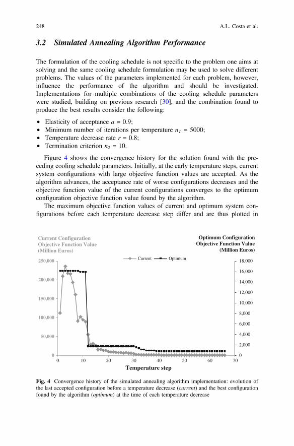
3.2 Simulated Annealing Algorithm Performance

The formulation of the cooling schedule is not specific to the problem one aims atsolving and the same cooling schedule formulation may be used to solve differentproblems. The values of the parameters implemented for each problem, however,influence the performance of the algorithm and should be investigated.Implementations for multiple combinations of the cooling schedule parameterswere studied, building on previous research [30], and the combination found toproduce the best results consider the following:

• Elasticity of acceptance a = 0.9;• Minimum number of iterations per temperature n1 = 5000;• Temperature decrease rate r = 0.8;• Termination criterion n2 = 10.

Figure 4 shows the convergence history for the solution found with the pre-ceding cooling schedule parameters. Initially, at the early temperature steps, currentsystem configurations with large objective function values are accepted. As thealgorithm advances, the acceptance rate of worse configurations decreases and theobjective function value of the current configurations converges to the optimumconfiguration objective function value found by the algorithm.

The maximum objective function values of current and optimum system con-figurations before each temperature decrease step differ and are thus plotted in

0

2,000

4,000

6,000

8,000

10,000

12,000

14,000

16,000

18,000

0

50,000

100,000

150,000

200,000

250,000

0 10 20 30 40 50 60 70

Temperature step

Current Optimum

Current Configuration Objective Function Value(Million Euros)

Optimum Configuration Objective Function Value

(Million Euros)

Fig. 4 Convergence history of the simulated annealing algorithm implementation: evolution ofthe last accepted configuration before a temperature decrease (current) and the best configurationfound by the algorithm (optimum) at the time of each temperature decrease

248 A.L. Costa et al.

different vertical scales. Both the current and optimum objective function valuesoverlap at the end of the algorithm if plotted on the same vertical scale. Theacceptance of configurations with large objective function values at the beginningof the algorithm is required for enabling the algorithm to globally explore thefeasible search space of the problem.

One observes that the objective function value of current configurations at theearly stages of the algorithm implementation is significantly larger than that ofthe best solution found. The relation between the high-speed rail configuration andthe deployment site characteristics substantiates this observation.

The three-dimensional limits for the deployment of the infrastructure are shownin Fig. 5. A reduced rectangular area of 147.4 * 304.4 km2 frames the plan view ofthe problem area and the elevation of the HSR is bounded by the depicted lowersurface and the top mesh. The lower elevation limit for the configuration corre-sponds to 50 m below sea level and the maximum corresponds to the maximumground elevation in the area.

It should be noted that construction costs can vary substantially within theproblem space. For example, a given HSR plan view can have multiple longitudinalprofiles corresponding to different extents of bridges and tunnels that, due to thelarge costs, can influence the overall infrastructure cost. Particularly for the cost ofbridges, the cost increases significantly with the increase in the infrastructure heightrelatively to the ground elevation. In addition to the construction costs, one verifiesif the design best practice geometry values are complied with and if the intermediatecities identified for the problem are connected. The respective values are added tothe construction cost to obtain the objective function value of any given systemconfiguration. Accordingly, high-speed rail configurations are found in the searchspace, which vary the objective function value in orders of magnitude.

Lisbon

CoimbraOporto

Elevation

0 - 10

10.1 - 250

250.1 - 450

450.1 - 730

730.1 - 1,411.16

Fig. 5 Three-dimensional limits for the deployment of the high-speed rail and the groundelevation (meters)

Application of the Simulated Annealing Algorithm … 249

Maier et al. in 2014 [44] discuss how large search space and complex fitnesslandscapes are characteristic of real-world problems. The fitness landscape dependson both the problem one aims at solving and the solving technique with therespective parameters implemented, defined by Smith et al. 2002 [45] as a multi-dimensional landscape established by the possible solutions the solving techniqueprogresses and correspondingly mapped to the respective fitness values.

Competing objectives are also characteristic of real-world problems. Forinstance, in the case of high-speed rail planning, optimizing the geometry layoutoften leads to larger construction costs that one aims at minimizing. This fact,coupled with the computational burden arising from the complexity and size ofreal-world problems, makes it difficult to identify the best convergence criteria [44].One observes in Fig. 4 that prior to the thirtieth temperature step, over ten tem-perature decreases occur without improvements in the best configuration found.But, as the current configurations are improving, the algorithm progresses untileventually in the thirty-first temperature step, the current optimum again improvesand converges to the best configuration found. The implementation of the termi-nation criteria should ensure that the algorithm does not terminate prematurely butalso that unnecessary computations are avoided and the algorithm terminates in afinite time [44].

The construction cost of the best configuration found, which connects twointermediate stations, is in line with existing high-speed rail lines in the world [12]and shows the ability of the simulated annealing algorithm in addressing theplanning of transport infrastructure. Further applications may be used to study howdifferent preferences for conflicting objectives influence the solutions obtained andsupport decision making.

4 Conclusions

This chapter discusses how the simulated annealing algorithm may be used toaddress the planning of transportation infrastructure. The specific case ofhigh-speed rail planning is discussed considering the location of intermediate sta-tions, the specific requirements of the infrastructure layout, and its interrelation withthe deployment site conditions. An application to a real-world case is presented thatexemplifies decisions regarding the simulated annealing implementation. Thesedecisions are discussed in light of existing research.

Ultimately, solving such real-world problems aims at supporting decisionmaking. This may be influenced by political decisions and based on the differentperspectives of multiple stakeholders. Providing only a single best solution for aparticular set of conditions is not adequate for decision making. The application ofthe optimization techniques for real-world problems should thus support theinvestigation of multiple opportunities and preferences for the problem at hand.

250 A.L. Costa et al.

Acknowledgments The authors would like to acknowledge the financial support of Fundaçãopara a Ciência e Tecnologia (FCT) through doctoral grant (SFRH/BD/43012/2008) and the accessto preliminary studies provided by former Rede Ferróviaria de Alta Velocidade, S.A. (RAVE).

References

1. Givoni, M., Rietveld, P.: Do cities deserve more railway stations? The choice of a departurerailway station in a multiple-station region. J. Transp. Geogr. 36, 89–97 (2014). doi:10.1016/j.jtrangeo.2014.03.004

2. Brons, M., Givoni, M., Rietveld, P.: Access to railway stations and its potential in increasingrail use. Transp. Res. Part A Policy Pract. 43, 136–149 (2009). doi:10.1016/j.tra.2008.08.002

3. Givoni, M., Rietveld, P.: The access journey to the railway station and its role in passengers’satisfaction with rail travel. Transp. Policy 14, 357–365 (2007). doi:10.1016/j.tranpol.2007.04.004

4. Repolho, H.M., Antunes, A.P., Church, R.L.: Optimal location of railway stations: theLisbon-Porto high-speed rail line. Transp. Sci. 47, 330–343 (2013). doi:10.1287/trsc.1120.0425

5. Vickerman, R.: High-speed rail in Europe: experience and issues for future development. Ann.Reg. Sci. 31, 21–38 (1997). doi:10.1007/s001680050037

6. Levinson, D.M.: Accessibility impacts of high-speed rail. J. Transp. Geogr. 22, 288–291(2012). doi:10.1016/j.jtrangeo.2012.01.029

7. EC: Commission Decision of 20 December 2007 concerning a technical specification forinteroperability relating to the infrastructure sub-system of the trans-European high-speed railsystem. Off. J. Eur. Union (2008)

8. CEN: Railway application—track alignment design parameters—track gauges 1435 mm andwider—Part 1: plain line. ENV 13803-1, CEN—European Committee for Standardization(2002)

9. RTRI: Design Standards for Railway Structures—Displacement Limits (2007)10. Levinson, D., Gillen, D., Kanafani, A., Mathieu, J.: The Full Cost of Intercity Transportation

—A Comparison of High Speed Rail, Air And Highway Transportation In California (1996)11. Levinson, D., Mathieu, J.M., Gillen, D., Kanafani, A.: The full cost of high-speed rail: an

engineering approach. Ann. Reg. Sci. 31, 189–215 (1997). doi:10.1007/s00168005004512. Campos, J., de Rus, G.: Some stylized facts about high-speed rail: a review of HSR

experiences around the world. Transp. Policy 16, 19–28 (2009). doi:10.1016/j.tranpol.2009.02.008

13. Jong, J.C.: Optimizing highway alignments with genetic algorithms. Ph.D. Dissertation.Department of Civil and Environmental Engineering (1998)

14. Jong, J.C., Jha, M.K., Schonfeld, P.: Preliminary highway design with genetic algorithms andgeographic information systems. Comput. Civ. Infrastruct. Eng. 15, 261–271 (2000)

15. Cheng, J.F., Lee, Y.S.: Model for three-dimensional highway alignment. J. Transp. Eng. 132,913–920 (2006). doi:10.1061/(asce)0733-947x(2006)132:12(913)

16. Lee, Y., Tsou, Y.R., Liu, H.L.: Optimization method forhighway horizontal alignment design.J. Transp. Eng. 135, 217–224 (2009). doi:10.1061/(ASCE)0733-947X(2009)135:4(217)

17. Jha, M.K.: Criteria-based decision support system for selecting highway alignments.J. Transp. Eng. 129, 33–41 (2003). doi:10.1061/(asce)0733-947x(2003)129:1(33)

18. Jha, M.K., Schonfeld, P.: A highway alignment optimization model using geographicinformation systems. Transp. Res. Part A Policy Pract. 38, 455–481 (2004). doi:10.1016/j.tra.2004.04.001

19. Kim, E., Jha, M.K., Schonfeld, P., Kim, H.S.: Highway alignment optimization incorporatingbridges and tunnels. J. Transp. Eng. 133, 71–81 (2007). doi:10.1061/(asce)0733-947x(2007)133:2(71)

Application of the Simulated Annealing Algorithm … 251

20. Fwa, T.F., Chan, W.T., Sim, Y.P.: Optimal vertical alignment analysis for highway design.J. Transp. Eng. 128, 395–402 (2002). doi:10.1061/(asce)0733-947x(2002)128:5(395)

21. Kim, E., Jha, M.K., Schonfeld, P.: Intersection construction cost functions for alignmentoptimization. J. Transp. Eng. 130, 194–203 (2004). doi:10.1061/(asce)0733-947x(2004)130:2(194)

22. Gipps, P.G., Gu, K.Q., Held, A., Barnett, G.: New technologies for transport route selection.Transp. Res. Part C Emerg. Technol. 9, 135–154 (2001). doi:10.1016/S0968-090X(00)00040-1

23. Jong, J.C., Schonfeld, P.: Cost functions for optimizing highway alignments. Transp. Res.Rec. J. Transp. Res. Board 1959, 58–67 (1999). doi:10.3141/1659-08

24. Parker, N.A.: Rural highway route corridor selection. Transp. Plan Technol. 3, 247–256(1977). doi:10.1080/03081067708717111

25. Trietsch, D.: A family of methods for preliminary highway alignment. Transp. Sci. 21, 17–25(1987)

26. Chew, E.P., Goh, C.J., Fwa, T.F.: Simultaneous optimization of horizontal and verticalalignments for highways. Transp. Res. Part B Methodol. 23, 315–329 (1989). doi:10.1016/0191-2615(89)90008-8

27. Kang, M.W., Jha, M.K., Schonfeld, P.: Applicability of highway alignment optimizationmodels. Transp. Res. Part C Emerg. Technol. 21, 257–286 (2012). doi:10.1016/j.trc.2011.09.006

28. Shafahi, Y., Bagherian, M.: A customized particle swarm method to solve highway alignmentoptimization problem. Comput. Civ. Infrastruct. Eng. 28, 52–67 (2013). doi:10.1111/j.1467-8667.2012.00769.x

29. Angulo, E., Castillo, E., Garcia-Rodenas, R., Sanchez-Vizcaino, J.: Determining highwaycorridors. J. Transp. Eng. 138, 557–570 (2012). doi:10.1061/(ASCE)TE.1943-5436.0000361

30. Costa, A.L., Cunha, C., Coelho, P.A.L.F., Einstein, H.H.: Solving high-speed rail planningwith the simulated annealing algorithm. J. Transp. Eng. 139, 635–642 (2013). doi:10.1061/(ASCE)TE.1943-5436.0000542

31. Metropolis, N., Rosenbluth, A.W., Rosenbluth, M.N., et al.: Equation of state calculations byfast computing machines. J. Chem. Phys. 21, 1087–1092 (1953)

32. Kirkpatrick, S., Gelatt, C.D., Vecchi, M.P.: Optimization by simulated annealing. Science 220,671–680 (1983)

33. Cerny, V.: Thermodynamical approach to the traveling salesman problem—an efficientsimulation algorithm. J. Optim. Theory Appl. 45, 41–51 (1985)

34. Aarts, E., Korst, J., Van Laarhoven, P.J.M.: Simulated annealing. In: Aarts, E., Lenstra, J.K.(eds.) Local Search in Combinatorial Optimization, 1st edn., pp 91–120. Wiley, New York(1997)

35. Dekkers, A., Aarts, E.: Global optimization and simulated annealing. Math. Program. 50, 367–393 (1991)

36. Johnson, D.S., Aragon, C.R., MCGeoch, L.A., Schevon C.: Optimization by simulatedannealing—an experimental evaluation. Part 1. Graph Partit. Oper. Res. 37, 865–892 (1989)doi:10.1287/opre.37.6.865

37. Osman, I.H., Laporte, G.: Metaheuristics: a bibliography. Ann. Oper. Res. 63, 513–623 (1996)38. Bertsimas, D., Nohadani, O.: Robust optimization with simulated annealing. J. Glob. Optim.

48, 323–334 (2010). doi:10.1007/s10898-009-9496-x39. Jilla, C.D., Miller, D.W.: Assessing the performance of a heuristic simulated annealing

algorithm for the design of distributed satellite systems. Acta Astronaut. 48, 529–543 (2001)40. Kirkpatrick, S.: Optimization by simulated annealing: quantitative studies. J. Stat. Phys. 34,

975–986 (1984). doi:10.1007/BF0100945241. APA: Environmental Atlas. In: Port. Environ. Agency (2012). http://sniamb.apambiente.pt/

webatlas/42. Cunha, M.C.: On solving aquifer management problems with simulated annealing algorithms.

Water Resour. Manag. 13, 153–169 (1999)

252 A.L. Costa et al.

43. Cunha, M.C., Sousa, J.J.O.: Hydraulic infrastructures design using simulated annealing.J. Infrastruct. Syst. 7, 32–39 (2001)

44. Maier, H.R., Kapelan, Z., Kasprzyk, J., et al.: Evolutionary algorithms and othermetaheuristics in water resources: current status, research challenges and future directions.Environ. Model Softw. 62, 271–299 (2014). doi:10.1016/j.envsoft.2014.09.013

45. Smith, T., Husbands, P., O’Shea, M.: Fitness landscapes and evolvability. Evol. Comput. 10,1–34 (2002). doi:10.1162/106365602317301754

Application of the Simulated Annealing Algorithm … 253

A Hybrid Bat Algorithm with PathRelinking for the Capacitated VehicleRouting Problem

Yongquan Zhou, Qifang Luo, Jian Xie and Hongqing Zheng

Abstract The capacitated vehicle routing problem (CVRP) is an NP-hard problemwith both engineering and theoretical interests. In this paper, a hybrid bat algorithmwithpath relinking (HBA-PR) isproposed to solveCVRP.TheHBA-PRisconstructedbased on the framework of the continuous bat algorithm, the greedy randomizedadaptive search procedure (GRASP) and path relinking are effectively integrated intothe bat algorithm.Moreover, in order to further improve the performance, the randomsubsequences and single-point local search are operated with certain loudness (aprobability). In order to verify the effectiveness of our approach and its efficiency andcompare with other existing methodologies, several classical CVRP instances fromthree classes of CVRP benchmarks are selected to test. Experimental results andcomparisons show the HBA-PR is effective for solving CVRPs.

Keywords Bat algorithm � Capacitated vehicle routing problem � Path relinking �GRASP � Metaheuristic algorithm

1 Introduction

The vehicle routing problem (VRP) is a classical combinatorial optimization prob-lem that was proposed in the late 1950s and it is still a research hotspot in the field ofOperations Research. The capacitated vehicle routing problem (CVRP) was intro-duced by Dantzig and Ramser in 1959 [1], which concerns that a set of customerdemands have to be served with a fleet of vehicles from a depot or central node, each

Y. Zhou (&) � Q. Luo � J. Xie � H. ZhengCollege of Information Science and Engineering, Guangxi University for Nationalities,Nanning 530006, Chinae-mail: yongquanzhou@126.com

Y. ZhouGuangxi High School Key Laboratory of Complex System and Computational Intelligence,Nanning 530006, China

© Springer International Publishing Switzerland 2016X.-S. Yang et al. (eds.), Metaheuristics and Optimization in Civil Engineering,Modeling and Optimization in Science and Technologies 7,DOI 10.1007/978-3-319-26245-1_12

255

vehicle has the uniform capacity and each customer has a certain demand that mustbe satisfied at the minimal cost. These costs usually represent the distances, travelingtimes, number of vehicles employed or a combination of these factors.

It is well-known that the CVRP is an NP-hard problem [2]. Various approacheshave been presented to solve the CVRP during the last decades, such as linearprogramming [3], several metaheuristics [4–6], and many hybrid heuristics withvariable neighborhood search or constructive heuristic methods [7–10]. The over-view of methods presented in [6] shows that at least 29 different methods forsolving CVRP exist, and all achieved more or less comparable performance.Although several methods can produce good solutions, the computational time islong when the scale of instances is large. Meanwhile, an abundance of methods forthe CVRP are population-based algorithms and the parameter setting of an algo-rithm is important, however, the parameter settings of many metaheuristics have notbeen considered in the literature.

The bat algorithm (BA) is a fairly new metaheuristic proposed by Yang [11, 25]in 2010, which inspired by the intelligent echolocation behavior of micro-bats whenthey forage. As we know, many new metaheuristics have been widely used andsuccessfully applied to solve the CVRP, though BA has not yet been applied tosolve the CVRP. However, BA has been applied to solve other problems with greatsuccess. For example, Gandomi et al. focus on solving constrained optimizationtasks [12]. Yang and Gandomi apply bat algorithm to solve many global engi-neering optimizations [13]. Mishra et al. proposed a model for classification usingthe bat algorithm to update the weights of a functional link artificial neural network(FLANN) classifier [14]. Meanwhile, some researchers have improved the batalgorithm and applied it to various optimization problems. Xie et al. proposed aDLBA bat algorithm based on differential operator and Lévy flights trajectory tosolve function optimization and nonlinear equations [15]. Wang et al. proposed anew bat algorithm with mutation (BAM) to solve the uninhabited combat airvehicle (UCAV) path planning problem [16]. In this paper, we propose a hybrid batalgorithm (HBA-PR) to solve the capacitated vehicle routing problem.

The rest of this paper is organized as follows. The problem of CVRP and theoriginal bat algorithm are described in Sect. 2. The hybrid bat algorithm (HBA-PR)for CVRP is described in Sect. 3. The experimental results of the HBA-PR andcomparisons with other previous algorithms are shown in Sect. 4. In the last section,we conclude this paper and point out some future work in Sect. 5.

2 Problem Descriptions and Bat Algorithm

2.1 Capacitated Vehicle Routing Problem

The CVRP is considered to be the classical version of the VRP which designs a setof customer demands that have to be served with a fleet of vehicles from a depot orcentral node, each vehicle has a uniform capacity, and each customer has a certain

256 Y. Zhou et al.

demand; the objective is to make the expended cost as low as possible. Let G ¼ðV ;EÞ be a complete graph with a set of vertices V ¼ f0; 1; . . .; kg; where thevertex {0} represents the depot and the remaining ones are the customers. Eachedge eij ¼ fi; jg 2 E has a non-negative cost cij and each customer i 2 V 0 ¼ Vnf0ghas a demand di. Let S ¼ ð1; 2; . . .;mÞ be the set of homogeneous vehicles withcapacity Q. The CVRP consists of constructing a set of up to k routes in such a waythat: (1) every route starts and ends at the depot; (2) all demands are accomplished;(3) the vehicle’s capacity is not exceeded; (4) a customer is visited by only a singlevehicle; and (5) the sum of costs is minimized. The mathematical formulas aredefined as follows [10].

min Z =Xki¼0

Xkj¼0

Xms¼0

cijeijs ð1Þ

s:t:Xki¼0

diyis �Q; s = 1,2,. . .m;

Xms¼1

yis ¼ 1; i = 1,2,. . .; k;

Xki¼0

eijs ¼ yis; j ¼ 1; 2; . . .; k; s ¼ 1; 2; . . .;m;

Xkj¼0

eijs ¼ yis; i ¼ 1; 2; . . .; k; s ¼ 1; 2; . . .;m

ð2Þ

where s denotes the number of vehicle, eijs ¼ 1 if vehicle s from i to j, otherwiseeijs ¼ 0; In addition, yis ¼ 1 if vehicle s is loading (active), otherwise yis ¼ 0.

2.2 Basic Bat Algorithm

The basic bat algorithm (BA) is a metaheuristic, first introduced by Yang in 2010.In simulations of BA, under several idealized rules, the updated rules of bats’positions xi and velocities vi in a D-dimensional search space are defined. The newsolutions xti and velocities vti at generation t are given by

fri ¼ frmin þðfrmax � frminÞbvti ¼ vt�1

i þðxt�1i � x�Þfri

xti ¼ xt�1i þ vti

ð3Þ

where b 2 ½0; 1� is a random vector drawn from a uniform distribution, fri denotesfrequency of each bat. Generally, the frequency is within a range, that is

A Hybrid Bat Algorithm with Path Relinking … 257

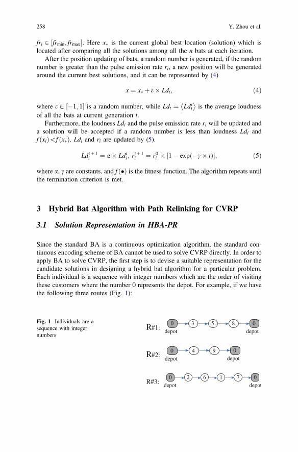
fri 2 ½frmin; frmax�. Here x� is the current global best location (solution) which islocated after comparing all the solutions among all the n bats at each iteration.

After the position updating of bats, a random number is generated, if the randomnumber is greater than the pulse emission rate ri, a new position will be generatedaround the current best solutions, and it can be represented by (4)

x ¼ x� þ e� Ldt; ð4Þ

where e 2 ½�1; 1� is a random number, while Ldt ¼ Ldti� �

is the average loudnessof all the bats at current generation t.

Furthermore, the loudness Ldi and the pulse emission rate ri will be updated anda solution will be accepted if a random number is less than loudness Ldi andf ðxiÞ\f ðx�Þ. Ldi and ri are updated by (5).

Ldtþ 1i ¼ a� Ldti ; r

tþ 1i ¼ r0i � ½1� expð�c� tÞ�; ð5Þ

where a, c are constants, and f �ð Þ is the fitness function. The algorithm repeats untilthe termination criterion is met.

3 Hybrid Bat Algorithm with Path Relinking for CVRP

3.1 Solution Representation in HBA-PR

Since the standard BA is a continuous optimization algorithm, the standard con-tinuous encoding scheme of BA cannot be used to solve CVRP directly. In order toapply BA to solve CVRP, the first step is to devise a suitable representation for thecandidate solutions in designing a hybrid bat algorithm for a particular problem.Each individual is a sequence with integer numbers which are the order of visitingthese customers where the number 0 represents the depot. For example, if we havethe following three routes (Fig. 1):

R#1:0

depot0

depot3 5 8

R#2:0

depot

0

depot4 9

R#3:70

depot

0

depot

2 6 1

Fig. 1 Individuals are asequence with integernumbers

258 Y. Zhou et al.

Where the coded individual with integers is 0 → 3 → 5 → 8 → 4 → 9 →2 → 6 → 1 → 7 → 0, and the bat individual is represented as 3 → 5 → 8 → 4 →9 → 2 → 6 → 1 → 7.

3.2 Hybrid Bat Algorithm

Aimed at the capacitated vehicle routing problem, based on the idea of the batalgorithm, a hybrid bat algorithm is proposed here, which integrates greedy ran-domized adaptive search procedure (GRASP) heuristic and the bat algorithm, andpath relinking as an intensification strategy to explore local trajectories connectingelite solutions obtained by the proposed algorithm. The hybrid bat algorithm withpath relinking is named as HBA-PR.

GRASP [17, 18] is a heuristic that has already been applied to many opti-mization problems successfully [19–21]. GRASP consists of a two phase iterativeprocess: a construction phase and a local search phase. In the first phase, a greedyrandomized solution is built. Since this solution is not guaranteed to be locallyoptimal, a local search is performed in the second phase. The final result is simplythe best solution found over all iterations.

The construction phase can be described as a process which stepwisely adds oneelement at a time to a partial (incomplete) solution. According to a greedy function,all elements are sorted, and the Restricted Candidate List (RCL) is constructedbased on the order; and then selects element randomly from this list. In the secondphase, a local search is initialized from these points, this iterative process is repe-ated until a termination criterion is met and the best solution found over all itera-tions is taken as the result.

RCL is created using a parameter a to restrict the size of this list. Candidatee 2 C is sorted according to their greedy function value f(e). In a cardinality-basedRCL, the latter is made up by the k top-ranked elements. In a value-based con-struction, the RCL consists of the elements in the set

fe 2 C : f� � f ðeÞ� f� þ a� ðf � � f�Þg ð6Þ

where f� ¼ minðf ðeÞ : e 2 CÞ; f � ¼ maxff ðeÞ : e 2 Cg; and a 2 ½0; 1�. Since thebest value for a is often difficult to determine, a random value is often assigned. Thevalues for a adopted in the constructive heuristics are set using reactive strategies,which usually leads to better performance than using fixed values [22].

In the original bat algorithm, the bat individual randomly selects a certain rangeof frequency, and its velocity is updated according to their selected frequency, atlast, a new position is generated using its velocity and its own position. The idea isthat the position of bat individual is updated by adjusting its frequency of sonicpulses. In this paper, the position updating of bat adopted GRASP to generate a new

A Hybrid Bat Algorithm with Path Relinking … 259

position, the frequency is used for restricting the size of CRL, frequency equivalentto parameter a in GRASP, and the frequency is a variable value. In the basic batalgorithm, the loudness Ld and the pulse emission rate r are updated accordingly asthe iterations proceed. As the loudness usually decreases, while the rate of pulseemission increases, it indicates the bats are approaching their prey (optimumsolution). The pulse emission rate r is updated by (7)

rðtÞ ¼ ð1þ expð5=tmax ��ðt � tmax=2ÞÞ�1; ð7Þ

where t denotes the tth generation, tmax is the maximal generation. The rate r issimilar to Sigmoid function, the frequency fr is determined according to the pulseemission rate r, which is represented by (8)

fr ¼ 1�maxð0:2;minð0:8; rÞÞ; rand[ r;maxð0:2;minð0:8; rÞÞ; rand� r;

�ð8Þ

where rand is a random number, and 0.2 and 0.8 are empirical parameters referencevalues [18]. The frequency fr decreases gradually at first, and then increasesgradually while the generation t increases. Figure 2 is the changing curve of rate r,and Fig. 3 is an example of frequency fr, and Algorithm 1 shows the pseudo-code ofgreedy randomized construction with frequency fr.

Algorithm1. Greedy_Randomized_Construction ( fr )

S Rrand_Chosen_ Vertex( v ); // Rrandomly chosen a vertex as initial solution\C V v ; // The candidate set C is initialized

While C ≠ ∅ doIC Evaluate_Incremental_Costs(S); // Incremental costs are evaluated

min min({ })ic ic IC∈ ;

max max({ })ic ic IC∈ ;

min max min{ | ( ) ( )}RCL e C ic e ic fr ic ic∈ ≤ + × − ; // RCL is created

s ← Select_Element (RCL); // a vertex s is randomly selected from RCLS Obtain_Min_Solution(S,s); // partial tour is updated by inserting vertex s

\{ }C C s ; // the candidate set C is updated

endreturn S

The local search phase uses the 2-Opt heuristic for exchanging. Algorithm 2shows the local search procedure. The input parameter is an initial solutionS obtained by the Greedy_Randomized_Construction procedure. The current routeneeds to divide into m sub-routes according to the load, the start, and the end ofsub-route is represented by 0, for example, S = {1, 2, 3, 4, 5, 6, 7}, sub-route is0 → 1 → 2 → 3 → 4 → 0, and 0 → 5 → 6 → 7 → 0.

260 Y. Zhou et al.

0 20 40 60 80 100 120 140 160 180 2000

0.1

0.2

0.3

0.4

0.5

0.6

0.7

0.8

0.9

1

iteration number

puls

e em

issi

on r

ate

r

Fig. 2 Changing curve of rate r

0 20 40 60 80 100 120 140 160 180 2000

0.1

0.2

0.3

0.4

0.5

0.6

0.7

0.8

0.9

1

iteration number

freq

uenc

y fr

Fig. 3 Changing curve of frequency fr

A Hybrid Bat Algorithm with Path Relinking … 261

Algorithm2. Local_Search_Phase ( S )

S S′ ;{ }sr Construct_Sub-route( S ′ );

for each sub-route sr dosr′ 2-opt ( sr ); // carry out the 2-opt operation

endS ′ Construct_Indiviaual({ }sr′ );

if ( ) ( )f S f S′ < then

S S ′endreturn S

3.3 Hybrid Bat Algorithm with Path Relinking

Path relinking was originally proposed by Glover [23], Laguna and Martı́ [24] werethe first to use path relinking within a GRASP strategy. Path relinking generatesnew solutions by exploring trajectories connecting an initial solution xs to an eliteguiding solution xt. The path relinking procedure consists of selecting moves thatintroduce attributes contained in the guiding solution xt to the initial solution xsuntil the initial solution is completely transformed in the guiding solution xt. Pathrelinking may also be viewed as a constrained local search strategy applied to theinitial solution xs. Furthermore, there are several alternatives that have been con-sidered, which involve some trade-offs between the computation time and solutionquality. These alternatives include periodical relinking, forward relinking, back-ward relinking, back and forward relinking, mixed relinking, randomized relinking,and truncated relinking [18].

One important issue in implementing a path relinking technique is the strategy toconstruct the elite set (ES). We adopted a fixed-size elite set and a solution x isinserted into the ES as follows.

A solution x is always inserted into ES if it is not full. Otherwise, the generatedsolution x is inserted in ES only if its cost is better than the worst cost solutionfound in ES, and the worst cost solution is replaced by the solution x. Algorithm 3shows the pseudo-code for the algorithm to construct and maintain the elite set ES.

262 Y. Zhou et al.

Algorithm 3. Elite _Set( x )

if ( )cardinality ES ps≠ then // ps is the population size

{ }ES ES x

else

wES the worst solution in ES

if ( ) ( )wf x f ES< then

\{ }wES ES ES

{ }ES ES x

endendreturn ES

Algorithm 4 shows the pseudo-code of path relinking procedure, an instance isxs ¼ 1; 2; 3; 4; 5; 6; 7f g, xt ¼ 1; 3; 4; 2; 5; 6; 7f g. According to the main process ofAlgorithm 4, the first different element is position 2 in xs, after executing areplacement operation, the new solution becomes x1 ¼ 1; 3; 4; 2; 5; 6; 7f g; thesecond different element is position 3 in xs, after executing the replacement oper-ation, the new solution is x2 ¼ 1; 2; 4; 3; 5; 6; 7f g. The third different element isposition 4 in xs, after executing the replacement operation, then x3. If x2 is only onebetter than xt, then x2 will be returned.

Algorithm 4. Path_Relinking( *ES , x );

sx x ; // initial solution

*tx ES ; // guiding solution

*( ) ( )tf x f ES ;

Difference( ,s tx x ); // find out the difference position between sx tx

for i=1: ( )cardinality Δ do

j Find_Position( , ,s t ix x Δ ); // find the position of the element of

tx in iΔ which in sx

ix Replace( , ,s ix jΔ ); // replace the j position of sx with the element of

sx in iΔ

ix Replace( , ,s t ix x Δ ); //replace the iΔ position of sx with the correspond-

ing element of tx

if ( ) ( )i tf x f x< then

* ix x ;

( ) ( )t if x f x ;

endendreturn *x

A Hybrid Bat Algorithm with Path Relinking … 263

3.4 Subsequence and Single-Point Local Search

In this paper, the loudness Ldi of bat individual i is related to its own fitness fiti, thebetter the fitness, and the lower the loudness. The loudness can be described by (9)

Ldi ¼ ðfiti � fit� þ 0:1Þ=ðfit� � fit� þ 0:1Þ; ð9Þ

where constant 0.1 is used for avoiding the denominator being zero. Here, fiti is thefitness of individual i, fit� and fit� are the minimum and maximum fitnesses incurrent population, respectively. In HBA-PR, the loudness reflects the quality of anindividual. In this algorithm, there are two kinds of local searches embedded intoHBA-PR to further improve the performance, and they are the random subsequencelocal search and the single-point local search. The random subsequence local searchincludes random subsequence inverse and random subsequence insertion, and thesingle-point local search includes single-point insert and single-point swap.

For a random subsequence insert, an origin of subsequence is randomly selectedat first, and then a length of subsequence is randomly selected, which is less thanthe length of individual S. Second, after determining the subsequence S1, a randominsertion point is selelcted in the remainder of subsequence S2, S ¼ S1[S2; andthen S1 is inserted into S2 location in the insert point. An example is shown inFig. 3. For the random subsequence inverse, a subsequence is randomly chosenwith a random length, and then the inverse operation is performed. An example isshown in Fig. 4.

For a single-point swap, two different positions are chosen from a permutationrandomly and are then swapped (Fig. 5). For a single-point insertion, two differentpositions are chosen from a permutation randomly and the element in the firstposition is inserted into the back of second element. Similarly, two instances areshown in Figs. 6 and 7.

In the local search part, the random subsequence local search is performedbefore random single-point local search. The random subsequence insert and therandom subsequence inverse operations are preformed according to loudness Ld. Inother words, if a random number is greater than the loudness Ldi; the randomsubsequence insert is performed; otherwise, the random subsequence inverse isperformed. Similarly, the random single-point insert and the random single-pointswap operations are preformed with the loudness Ld. If a random number is greaterthan the loudness Ldi; the insert operation is performed; otherwise, the swapoperation is performed. Note that, where a local search is operated on the currentoptimal individual ES� in elite set ES, and a local search is performed for eachindividual. Algorithms 5 and 6 show the pseudocodes of the subsequence andsingle-point local search.

264 Y. Zhou et al.

7

0

depot

0

depot

2 6 1 3 5 8 4

12 6 8 7 3 5 4

First element

Before

After

Random Insert Position is (7,2)Second elementSecond element First element

Fig. 7 Single-point insert operation

7

0

depot

0

depot

2 6 1 3 5 8 4

72 8 1 3 5 6 4

First element

Before

After

Random Swap Position is (7,2) Second elementSecond elementFirst element

Fig. 6 Single-point swap operation

7

0 0

depot

2 6 1 3 5 8 4

72 5 3 1 6 8 4

Sub-sequence

Before

After

depotSub-sequence

Fig. 5 Random subsequence inverse operation

7

0

depot

0

depot

2 6 1 3 5 8 4

62 5 8 1 7 3 4

Sub-sequenceInsert point

Sub-sequence

Before

After

Fig. 4 Random subsequence insert operation

A Hybrid Bat Algorithm with Path Relinking … 265

Algorithm 5. Sub-sequence_ Local_Search ( *ES )

for i=1:ps doif rand> iLd then

x Sub-sequence_Insert( *ES ); // perform random sub-sequence in-

sert operationelse

x Sub-sequence_ Inverse( *ES ); // perform random sub-sequence in-

verse operationend

endreturn x

Algorithm 6. Single-point_Local_Search ( *ES )

for i=1:ps doif rand> iLd then

x Single-point_Insert( *ES ); // perform random single-point insert operation

elsex Single-point_Swap( *ES ); // perform random single point swap operation

endendreturn x

3.5 HBA-PR Framework for CVRP

We propose in this work to incorporate the greedy randomized adaptive searchprocedure, path relinking strategies, subsequence, and single-point local search tothe bat algorithm by defining distinct ways to solve the capacitated vehicle routingproblem. This iterative process is repeated until the termination criterion is met,Algorithm 7 shows the pseudocode of HBA-PR for CVRP.

266 Y. Zhou et al.

Algorithm 7. HBA-PRInitialize the ps ,bat population and other parameters ;

Evaluate fitness for each individual;

ES Elite _Set( x );

while t<tmax doCompute pulse emission rate by (6);

Determine frequency fr by (7);

for i=1:ps dox Greedy_Randomized_Construction( fr );

x Local_Search_Phase ( x );

endEvaluate fitness for each individual x ;

ES Elite _Set( x );

*ES Select_Best_Elite( ES ); // select the best individual in

elite set ESfor i=1:ps do

x Path_Relinking( *ES , x);

endEvaluate fitness for each individual x ;

ES Elite _Set( x );

iLd Compute_Loudness( ( )f x ) ; //Compute loudness of each

individual by (8);

*ES Select_Best_Elite( ES );

x Sub-sequence_ Local_Search ( *ES ) //carry out random sub-

sequence local searchEvaluate fitness for each individual x ;

ES Elite _Set( x );

*ES Select_Best_Elite( ES );

x Single-point_Local_Search ( *ES ) //carry out random sin-

gle-point local searchEvaluate fitness for each individual x ;

ES Elite _Set( x );

t=t+1

endOutput result and plot

A Hybrid Bat Algorithm with Path Relinking … 267

4 Numerical Simulation Results and Comparison

The performance of the proposed HBA-PR is extensively tested by a large numberof experimental studies; computational simulations are carried out with somewell-studied problems taken from the web http://www.branchandcut.org/, a refer-ence site which contains some detailed information regarding a large number ofbenchmark instances. In this paper, 12 instances from three classes of benchmarksare selected. The first class is Augerat et al. (Set A) instances. The second class isAugerat et al. (Set P) instances, and the third class is Augerat et al. (Set E)instances. So far, these problems have been widely used as the benchmarks tovalidate the performance of algorithms by many researchers.

All computational experiments are conducted with MATLAB 2012a, and in oursimulations, numerical experiments are run on a PC with AMD Athlon(tm) II X4640 Processor 3.0 GHz and 2.0 GB memory. In the experiment, the terminationcriterion is set as the maximum generation of tmax ¼ 200. Each instance is inde-pendently run 15 times for comparison.

4.1 Parameter Analysis

In the subsection, the parameters of HBA-PR are determined by experiments, andthe impact of each parameter is analyzed. In particular, the HBA-PR has fewparameters; we only need to test population size ps in HBA-PR. A small ps maylead to insufficient population information, and the diversity cannot be guaranteed.On the other side, a large one indicates that diversity is sufficient, but the computingtime will increase and the precision of the optimal solution may have lesserimprovement. In order to evaluate the sensitivity of parameters ps, three bench-marks selected from different benchmark set are chosen to run 10 times. Thesebenchmarks are A_n33_k5, E_n23_k3, and P_n19_k2, and the statistical result andconvergence curves are shown in Figs. 8, 9, 10 and 11.

The ordinate normalized fitness (log) in Figs. 8, 9 and 10 is the logarithm ofnormalized fitness; the aim is to show the convergence curves clearly. The nor-malization formula of fitness is ðfit� fit�Þ=ðfit� � fit�Þ, where fit� is the best-knownsolution and fit� is the initial fitness.

Figure 8 represents the relative error of test case A_n33_k5, E_n23_k3 andP_n19_k2 after 10 times independent runs, which shows that the sensitivity ofparameter ps. From the three test cases, the parameter ps can be determined. ForA_n33_k5 and P_n19_k2, the performance of HBA-PR is better when ps = 30. ForE_n23_k3, ps = 50 is best, but the performance is good as well while ps = 30. FromFigs. 8, 9 and 10, the information provided by population is sufficient when ps isgreater than 20; however, the convergence rate is better when ps = 30 among thethree instances. Considering the tradeoff between the stability of the algorithm andthe rate of convergence, the parameter ps took a compromising value, ps = 30.

268 Y. Zhou et al.

670

680

690

ps=10 ps=20 ps=30 ps=40 ps=50

fitne

ss

A-n33-k5

568570572574576578

ps=10 ps=20 ps=30 ps=40 ps=50

fitne

ss

E-n23-k3

212214216218220222

ps=10 ps=20 ps=30 ps=40 ps=50

fitne

ss

P-n19-k2

Fig. 8 Box-and-whisker diagram of selected three instances

0 20 40 60 80 100 120 140 160 180 20010

-3

10-2

10-1

100

Iterations

Nor

mal

ized

fitn

esss

(Lo

g)

ps=10

ps=20

ps=30ps=40

ps=50

Fig. 9 Convergence curve for A_n33_k5

A Hybrid Bat Algorithm with Path Relinking … 269

4.2 Comparisons of Simulation Results

In order to show the effectiveness of HBA-PR, we carry out a set of simulations tocompare HBA-PR with other state-of-the-art algorithms, i.e., a parallel version ofthe classical Clarke and Wright Savings (CWS) heuristic, SR-GCWS (Simulation in

0 20 40 60 80 100 120 140 160 180 200

10-3

10-2

10-1

100

Iterations

Nor

mal

ized

fitn

esss

(Lo

g)ps=10ps=20ps=30ps=40ps=50

Fig. 10 Convergence curve for E_n23_k3

0 20 40 60 80 100 120 140 160 180 200

10-1

100

Iterations

Nor

mal

ized

fitn

esss

(Lo

g)

ps=10

ps=20

ps=30

ps=40

ps=50

Fig. 11 Convergence curve for P_n19_k2

270 Y. Zhou et al.

Tab

le1

Com

parisonof

results

forAug

erat

etal.SetA,E,andPinstances

Instance

Capacity

Tight-ness

I_BKS

R_B

SKCWS

SR-G

CWS

CS-GRASP

HBA-PR

A-n33

-k5

100

0.89

661

662.76

712.05

662.11

662.14

5266

2.11

01

A-n33

-k6

100

0.9

742

742.83

776.26

742.69

743.57

8574

2.69

33

A-n37

-k5

100

0.81

669

672.59

707.26

672.47

672.46

5267

2.46

52

A-n39

-k6

100

0.88

831

833.20

863.08

833.20

–83

5.25

18

E-n23

-k3

4500

0.75

569

––

–56

9.74

6156

8.56

25

E-n22

-k4

6000

0.94

375

375.28

388.77

375.28

–37

5.27

98

E-n33

-k4

8000

0.92

839

838.72

843.1

837.67

–83

7.92

53

E-n51

-k5

160

0.97

521

524.94

584.64

524.61

–52

4.61

11

P-n1

9-k2

160

0.97

212

212.66

237.90

212.66

212.65

6921

2.65

69

P-n2

0-k2

160

0.97

216

217.42

234.00

217.42

217.41

5621

7.41

56

P-n2

2-k2

160

0.96

216

217.85

239.50

217.85

217.85

2221

7.85

22

P-n5

1-k1

080

0.97

741

742.48

790.97

741.50

–74

3.26

48

A Hybrid Bat Algorithm with Path Relinking … 271

Routing via the Generalized Clarke and Wright Savings heuristic) proposed by Juanet al. [9], CS-GRASP proposed by Zheng et al. [10]. The results of these simula-tions are summarized in Table 1 which contains the following information of eachinstance: Vehicle Capacity, Tightness (Demand/Capacity), I_BKS is integralbest-known solution (BKS) or ‘optimal’ value according to the web http://www.branchandcut.org/. R_BSK is verified by the real costs for the best-known solutionsaccording to [9] and CWS is the costs associated with the solution given by theparallel version of the CWS heuristic, while SR-GCWS is the best solution obtainby SR-GCWS method, and HBA-PR is our best solution, where “–” represents norecords in the literature.

From the simulation results obtained by testing HBA-PR, it demonstrates thatthe proposed HBA-PR is effective to solve the CVRP, and the performance ofHBA-PR is prominent. From Table 1, all instances achieved a good quality solu-tion, and the solutions of six instances are better than the best-known solutions(‘optimal’ value). HBA-PR has matched 10 of the 12 best-known solutions exceptfor P_n51_k10 and A_n39_k6, and the average deviation from the real costsbest-known solutions is 0.057 %. HBA-PR outperforms CWS for the 12 instances.Compare with CS-GRASP and HBA-PR, HBA-PR outperform CS-GRASP interms of A_n33_k5, A_n33_k6 and E_n23_k3, the other instances have sameresults. The SR-GCWS and HBA-PR have similar results, and the gap is very small.

Furthermore, Fig. 12 shows the best solution found so far by using ourmethodology for the A_n37_k5.vrp file, where the depot (using 1 instead of 0) is at

10 20 30 40 50 60 70 80 90 100

0

10

20

30

40

50

60

70

80

90

1 23

4

5

6 7

8

9

10

11

12

13

14

15

16

17

18

19

20

21

22

23

24

25

26

27

28

29

30

3132

33

34

35

36

37

Fig. 12 Optimal routes of A_n37_k5

272 Y. Zhou et al.

the center. Analogously, Figs. 13, 14 and 15 show the best solutions found byHBA-PR for the E-n51-k5.vrp file and P_n51_k10.vrp file. The convergence curvefor some test problems has been shown in Fig. 14. From Fig. 14, for e.g.,A_n37_k5, it converges to an optimal solution after 43 generations, and it expends

0 10 20 30 40 50 60 700

10

20

30

40

50

60

70

1

23

4

5

6

7

8 9

10

11

12

13

14

15

16

17

18

19

20

21

22

2324

25

26

27

28

29

30

31

32

33

34

35

36

37

38

39

40

41

42

43

44

45

46

47

48

49

50

51

Fig. 13 Optimal routes of E_n51_k5

0 10 20 30 40 50 60 700

10

20

30

40

50

60

70

1

23

4

5

6

7

8 9

10

11

12

13

14

15

16

17

18

19

20

21

22

2324

25

26

27

28

29

30

31

32

33

34

35

36

37

38

39

40

41

42

43

44

45

46

47

48

49

50

51

Fig. 14 Optimal routes of P_n51_k10

A Hybrid Bat Algorithm with Path Relinking … 273

about 170 generations; for e.g., E-n51-k5 and P_n51_k10 when the algorithmconverges to an optimal solution, which demonstrates that the HBA-PR has a fasterconvergence rate.

In general, the proposed HBA-PR can produce good solutions when comparedwith existing heuristics for solving the CVRP, and the convergence rate of HBA-PRis faster. These results seem to indicate that the hybrid bat algorithm with pathrelinking is an effective alternative to solve the capacitated vehicle routing problem.

5 Conclusions

The capacitated vehicle routing problem is important in the fields of operationsresearch, which is an NP-hard problem. The bat algorithm is a continuous meta-heuristic that cannot be used to solve the CVRP directly. In this paper, a hybrid batalgorithm with path relinking (HBA-PR) for solving the CVRP has been presented.This methodology, which does not require any particular fine-tuning of parametersor configuration process, combines the classical greedy randomized adaptive searchprocedure (GRASP) with the bat algorithm, and path relinking as an intensificationstrategy to explore local trajectories connecting elite solutions obtained by proposedalgorithm; sub-sequence and single-point local searches are effectively integratedinto HBA-PR. The results show that our methodology is able to provide fine-qualitysolutions which can compete with the ones provided by some exact and heuristicapproaches. Moreover, because of its simplicity and flexibility, we believe that thismethodology can easily be adapted to solve other variants of the vehicle routing

0 20 40 60 80 100 120 140 160 180 200

600

800

1000

1200

1400

1600

1800

Iterations

Fitn

ess

A-n37-k5

E-n51-k5

P-n51-k10

Fig. 15 Convergence curve of three instances

274 Y. Zhou et al.

problem and even to other combinatorial problems, for example, the vehicle routingproblem with time windows and the well-known traveling salesman problem,which will form part of our further work.

Acknowledgments This work is supported by the National Science Foundation of China underGrants No.s 61165015 and 61463007. The Key Project of Guangxi Science Foundation underGrant No. 2012GXNSFDA053028, Key Project of Guangxi High School Science Foundationunder Grant No. 20121ZD008.

References

1. Dantzig, G., Ramser, J.H.: The truck dispatching problem. Manag. Sci. 6, 80–91 (1959)2. Haimovich, M., Rinnooy Kan, A.H.G., Stougie, L.: Analysis of heuristics for vehicle routing

problems. In: Golden, B.L., Assad, A.A. (eds.) Vehicle Routing: Methods and Studies.Elsevier, Amsterdam, North-Holland (1988)

3. Toth, P., Tramontani, A.: An integer linear programming local search for capacitated vehiclerouting problems. In: The Vehicle Routing Problem: Latest Advances and New Challenges,pp. 275–295. Springer, New York (2008)

4. Nazif, H., Lee, L.S.: Optimised crossover genetic algorithm for capacitated vehicle routingproblem. Appl. Math. Model. 36(5), 2110–2117 (2012)

5. Ai, T.J., Kachitvichyanukul, V.: Particle swarm optimization and two solution representationsfor solving the capacitated vehicle routing problem. Comput. Ind. Eng. 56(1), 380–387 (2009)

6. Szeto, W.Y., Wu, Y.Z., Ho, S.C.: An artificial bee colony algorithm for the capacitated vehiclerouting problem. Eur. J. Oper. Res. 215(1), 126–135 (2011)

7. Chen, P., Huang, H.K., Dong, X.Y.: Iterated variable neighborhood descent algorithm for thecapacitated vehicle routing problem. Expert Syst. Appl. 37(2), 1620–1627 (2010)

8. Yurtkuran, A., Emel, E.: A new Hybrid Electromagnetism-like Algorithm for capacitatedvehicle routing problems. Expert Syst. Appl. 37(4), 3427–3433 (2010)

9. Juan, A.A., Faulin, J., Ruiz, R., Barrios, B., Caballé, S.: The SR-GCWS hybrid algorithm forsolving the capacitated vehicle routing problem. Appl. Soft Comput. 10(1), 215–224 (2010)

10. Zheng, H.Q., Zhou, Y.Q., Luo, Q.F.: A hybrid cuckoo search algorithm-GRASP for vehiclerouting problem. J. Convergence Inf. Technol. 8(3) (2013)

11. Yang, X.S.: A new metaheuristic bat-Inspired algorithm. Nature Inspired CooperativeStrategies for Optimization (NICSO). SCI 284, B65–B74 (2010)

12. Gandomi, A.H., Yang, X.S., Alavi, A.H., Talatahari, S.: Bat algorithm for constrainedoptimization tasks. Neural Comput. Appl. 1–17 (2012)

13. Yang, X.S., Gandomi, A.H.: Bat algorithm: a novel approach for global engineeringoptimization. Eng. Comput. 29, 464–483 (2012)

14. Mishra, S., Shaw, K., Mishra, D.: A new meta-heuristic bat inspired classification approach formicroarray data. Procedia Technol. 4, 802–806 (2012)

15. Xie, J., Zhou, Y.Q., Chen, H.: A novel bat algorithm based on differential operator andLévy-flights trajectory. Comput. Intell. Neurosci. http://dx.doi.org/10.1155/2013/453812(2013)

16. Wang, G., Guo, L., Duan, H., Liu, L., Wang, H.: A bat algorithm with mutation for UCAVpath planning. Sci. World J. http://dx.doi.org/10.1100/2012/418946 (2012)

17. Feo, T., Resende, M.: Greedy randomized adaptive search procedures. J. Global Optim. 6(2),109–133 (1995)

18. Resendel, M.G.C, Ribeiro, C.C.: GRASP with path-relinking: recent advances andapplications. In: Metaheuristics: Progress as Real Problem Solvers, pp. 29–63. Springer,New York (2005)

A Hybrid Bat Algorithm with Path Relinking … 275

19. Festa, P., Resende, M.: An annotated bibliography of GRASP, part I: algorithms. Int. Trans.Oper. Res. 16, 1–24 (2009)

20. Festa, P., Resende, M.: An annotated bibliography of GRASP, Part II: Applications. Int.Trans. Oper. Res. 16, 131–172 (2009)

21. Mestria, M., et al.: GRASP with path relinking for the symmetric euclidean clustered travelingsalesman problem. Comput. Oper. Res. http://dx.doi.org/10.1016/j.cor.2012

22. Resende, M.G.C., Ribeiro, C.C., Glover, F., Mart, R.: Scatter search and path-relinking:fundamentals, advances, and applications. In: Gendreau, M., Potvin, J.Y. (eds) Handbook ofMetaheuristics, pp. 87–107. Springer, Boston (2010)

23. Glover, F.: Tabu search and adaptive memory programming–advances, applications andchallenges. In: Barr, R.S., Helgason, R.V., Kennington, J.L. (eds.) Interfaces in ComputerScience and Operations Research, pp. 1–75. Kluwer, Dordrecht (1996)

24. Laguna, M., Martı́, R.: GRASP and path relinking for 2-layer straight line crossingminimization. J. Comput. 11(1), 44–52 (1999)

25. Bekdaş, G., Nigdeli, S.M., Yang, X.-S.: Metaheuristic optimization for the design ofreinforced concrete beams under flexure moments. In: 5th European Conference of CivilEngineering (ECCIE’14), 22–24 Nov 2014, Florence, Italy

276 Y. Zhou et al.

Hybrid Metaheuristic Algorithmsin Geotechnical Engineering

Y.M. Cheng

Abstract The solutions of many engineering problems can be formulated as theoptimized results of a functional. While many engineering problems are governedby a continuous convex optimization process, this is not the case for manygeotechnical problems. Many geotechnical problems have irregular solutiondomains, with the objective function being nonconvex and may not be a continuousfunction. The presence of multiple local minima is common in many geotechnicalproblems, and the occurrence of local zones where there is rapid changes in thematerial parameters is not uncommon. The corresponding governing problems arehence usually NP-type nonconvex optimization problem, and by nature, suchNP-type problems with the various constraints pose great difficulty in analysis.While the classical heuristic optimization methods may work well for some of theseproblems, there are also some practical cases where the classical methods may failto perform satisfactorily. To maintain a balance between the computation time andaccuracy, several hybrid metaheuristic algorithms are proposed by the author whichcan work well for many practical geotechnical problems. In this chapter, the authorwill illustrate the basic concept of hybrid metaheuristic algorithms and the appli-cations to some difficult geotechnical problems.

Keywords Hybrid optimization � Geotechnical engineering � Wave equation �Back analysis � Slope stability

1 Introduction

In the solution of many engineering problems, many numerical methods have beendeveloped over the years. The finite element method is the most popular numericalmethod at present due to its versatility in many complicated problems. The fun-

Y.M. Cheng (&)Department of Civil and Environmental Engineering,Hong Kong Polytechnic University, Hung Hom, Hong Konge-mail: ceymchen@polyu.edu.hk

© Springer International Publishing Switzerland 2016X.-S. Yang et al. (eds.), Metaheuristics and Optimization in Civil Engineering,Modeling and Optimization in Science and Technologies 7,DOI 10.1007/978-3-319-26245-1_13

277

damental principle of the finite element is either the variational formulation or theGalerkin formulation [1], which can be viewed as the minimization of energy orfunctional. The determination of the shortest path, minimum functional or energy isrequired for many stability problems in geotechnical engineering, as the ultimatecondition will provide the factor of safety for use by many engineers. While Denn[2] has demonstrated that the variational principle can be used for optimizationanalysis, Cheng et al. [3] and Cheng [4] have demonstrated that the optimizationprocess is equivalent to the variational principle and can replace it for use in avariety of problems. Due to the needs for the determination of the optimizedsolution for various engineering problems, different methods have been proposedwith success in different disciplines. Traditionally, resource allocation, packing, andscheduling as well as many other similar problems are analyzed using linear and/orinteger programming method. Such methods usually require the objective functionand constraints to be linear functions, but the optimum solution can usually bedetermined rapidly (except under very special cases). Various gradient-typemethods have been proposed and used for many engineering problems, and theFSQP (Feasible sequential quadratic programming) and BFGS (Broyden–Fletcher–Goldfarb–Shanno) methods which are variants of the quasi-Newton approachappear to be very effective in many situations with very good performance. Suchgradient-type methods require the differentiability of the objective functions (can beformed by finite difference scheme) are, however, limited by the continuityrequirement, and the global minimum may not be determined unless a good initialis used in the analysis. In geotechnical engineering and many other disciplineswhere multiple minima exist in the solution domain, the uses of the previous twogroups of methods are seldom adopted. The author has, however, used these typesof methods for global optimization in some geotechnical problems by specifying aseries of initial starting points, and such strategy appears to be necessary for somelarge-scale systems where the numbers of variables are in the order of thousands.

In general, most of the practical engineering problems are constrained withinacceptable solution domain. The objective functions in many geotechnical ortransportation problems are usually NP (nonpolynomial) hard-type problems withthe features:

• The solution domain and/or the problem geometry are not regular and smooth.The objective function is commonly nonsmooth and nonconvex, it may not becontinuous within the part of the solution domain (failure to converge orinfeasible solution).

• Multiple local minima will be present in general, and a good initial trial can bedifficult to be specified for general cases. For the one-dimensional functiondefined over the domain AB as shown in Fig. 1, the global minimum is given bypoint E, but points C and D may also be obtained if the optimization algorithmcannot escape from the local minimum. If the global minimum is governed bypoint B where the derivative of the function is not zero, many optimizationalgorithms (particularly those gradient types) will fail to detect this point.

278 Y.M. Cheng

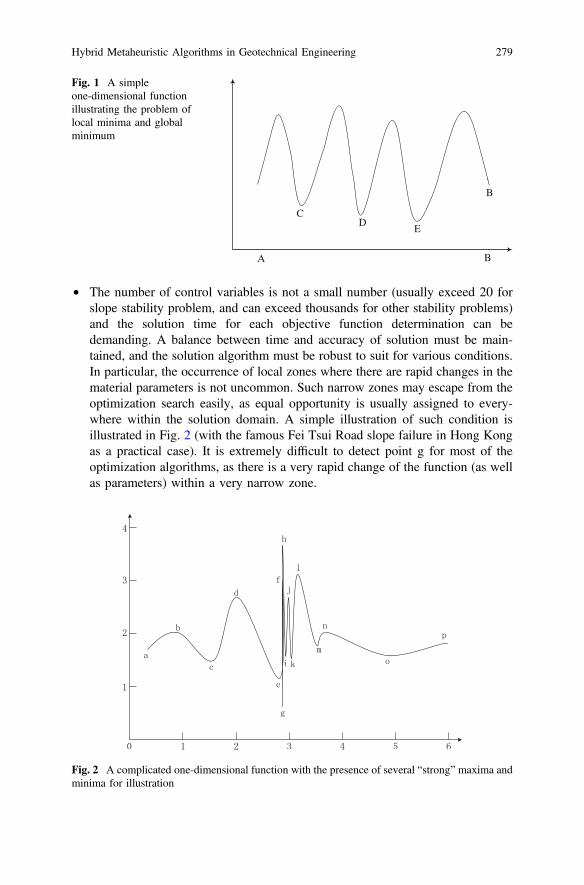
• The number of control variables is not a small number (usually exceed 20 forslope stability problem, and can exceed thousands for other stability problems)and the solution time for each objective function determination can bedemanding. A balance between time and accuracy of solution must be main-tained, and the solution algorithm must be robust to suit for various conditions.In particular, the occurrence of local zones where there are rapid changes in thematerial parameters is not uncommon. Such narrow zones may escape from theoptimization search easily, as equal opportunity is usually assigned to every-where within the solution domain. A simple illustration of such condition isillustrated in Fig. 2 (with the famous Fei Tsui Road slope failure in Hong Kongas a practical case). It is extremely difficult to detect point g for most of theoptimization algorithms, as there is a very rapid change of the function (as wellas parameters) within a very narrow zone.

CD

E

B

A B

Fig. 1 A simpleone-dimensional functionillustrating the problem oflocal minima and globalminimum

Fig. 2 A complicated one-dimensional function with the presence of several “strong” maxima andminima for illustration

Hybrid Metaheuristic Algorithms in Geotechnical Engineering 279

Due to the special requirements of the objective functions in geotechnical engi-neering, many researchers have adopted different methods to search for the globalminimum in geotechnical engineering with various success and limitations. Finiteelement limit analysis usually adopts those gradient-type methods with the use ofdifferent initial solutions in the optimization analysis. Slope stability problem iscontrolled by limitation 1 as given above, and the gradient-type method is virtuallynot adopted in practice. For such problems, heuristic optimization methods are morepopular at present, and a detailed discussion is given by Cheng [5], Cheng and Li [6],Cheng et al. [7], Cheng et al. [8, 9]. Themodern heuristic global optimizationmethodshave attracted the attention of many geotechnical engineers recently due to the sim-plicity in implementation, satisfactory performance in many practical problems, andincreased speed in solution when the number of variables is not excessive. At present,simulated annealing, tabu search, genetic algorithm, particle swarm optimization, fishswarm optimization, harmony search, ant colony method, evolution algorithm, andmany other similar variants have been adopted in many geotechnical problems withsatisfaction. These methods are suitable for medium-size problems with the presenceof multiple local minima. Cheng et al. [7] have carried out a detailed comparisonbetween six major types of heuristic global optimization methods in slope stabilityproblem, and has concluded that no single method can outperform other methodsunder all cases. Thatmeans, everymethod has its own advantages and limitations, andthere is no single method which is universal and can perform well under all cases.A good optimization algorithm should preferably be insensitive to the optimizationparameters, except for some very special cases. The author has also carried out thesensitivity analysis of these methods under different optimization parameters which isa very useful and important work but is not commonly considered. It is also observedthat some optimization methods (ant colony and tabu search) may be less effective forproblem where the objective functions are highly discontinuous, but may be highlyefficient when the problem is relatively simple.

2 Example of Geotechnical Problems Which RequireHeuristic Optimization Analysis

There are many geotechnical problems which require the use of optimizationanalysis, in particularly, the pile driving and stability problems. The control of piledriving and the evaluation of the pile capacity are important for pile installation.Currently, there is an increasing trend to adopt the dynamic test instead of theclassical kentledge test in order to save the cost of testing as well as examiningmore piles. The pile driving wave equation for a uniform pile is given by:

@2u@t2

¼ C2 @2u

@x2þR ð1Þ

280 Y.M. Cheng

where u is the axial displacement which is a function of both the depth x and time t,C is the speed of stress wave, R is the skin resistance of soil around the pile which isa function of x and t. Based on the theory of characteristics, the integral along thepositive and negative directions of the characteristics line gives the followingiterative form:

Alongdxdt

¼ C; Zi�1Vi;j þFi;j ¼ Zi�1Vi�1j þFi�1j � Rþi�1 ð2Þ

Alongdxdt

¼ �C; ZiVi;j � Fi;j ¼ ZiViþ 1;j�1 þFiþ 1;j�1 � R�i ð3Þ

whereRþi�1 ¼

Ru i� 1ð ÞOk i� 1ð Þ ui�1j � upi�1j

� �1þ Jsi�1Vi�1;j� � ð4Þ

R�i ¼ Ru ið Þ

Qk ið Þ uiþ 1;j�1 � upiþ 1;j�1� �

1þ JsiViþ 1;j�1� � ð5Þ

Z, V, F, Q, Ru, Q, and J are the impedance, velocity of wave, force in pile, elasticlimit of skin friction, ultimate skin resistance, quake, and damping constant of theSmith model, respectively (see [10] for details). After a time interval Dt, upwardPu i� 1; jð Þ and downward traveling waves Pd i� 1; j� 1ð Þ become Pði;jÞ at the topof the unit. When t ¼ jDt, considering the transmission and reflection of the upwardand downward traveling waves, and the upward and downward traveling waves ofthe skin resistance R i; tð Þ, the upward and downward traveling waves at sectioni are, respectively, given as follows:

Pu i; jð Þ ¼ 2 � ZiZiþ 1 þ Zi

Pu iþ 1; jð Þþ Ziþ 1 � ZiZiþ 1 þ Zi

Pd i; j� 1ð Þþ ZiZi�1 þ Zi

R i; jð Þ ð6Þ

Pd i; jð Þ ¼ 2 � ZiZi þ Zi�1

Pu i� 1; j� 1ð Þþ Zi�1 � ZiZi þ Zi�1

Pu i; j� 1ð Þ � Ziþ 1

Zi þ Ziþ 1R i; jð Þ

ð7Þ

At the pile tip, the upward and downward traveling waves will be:

Pd Np;j� � ¼ Pd Np�1;j�1

� � ð8Þ

Pu Np;j� � ¼ �Pd Np�1;j�1

� �þR Ns;j� �þR Nsþ 1;j

� � ð9Þ

At time t, the measured force and speed near to the top of pile are Pm jð Þ and Vm jð Þ.If we take the location of the PDA sensors as the boundary and the measure velocityas the boundary condition to compute the force in pile, we have

Hybrid Metaheuristic Algorithms in Geotechnical Engineering 281

Pu 1; jð Þ ¼ Pu 2; j� 1ð Þ ð10Þ

Pd 1; jð Þ ¼ ZVm jð ÞþPuð2; j� 1Þ ð11Þ

Therefore, the force–time curve can be obtained by:

Pc jð Þ ¼ Pd i; jð ÞþPu i; jð Þ ¼ ZVm jð Þþ 2Pu 2; j� 1ð Þ ð12Þ

The particle velocity and displacement V i; jð Þ and S i; jð Þ are given by:

V i; jð Þ ¼ Pd i; jð ÞZi

� Pu i; jð ÞZiþ 1

ð13Þ

S i; jð Þ ¼ S i; j� 1ð Þþ Dt2

V i; j� 1ð ÞþV i; jð Þ½ � ð14Þ

If the Smith soil model is used, three parameters will be defined: the maximumstatic resistance Ru, the largest elastic deformation Q, and the Smith dampingcoefficient Js. Soil resistance Rði; jÞ is divided into static resistance Rsði; jÞ anddynamic resistance Rdði; jÞ as given by

R ið Þ ¼ Rs i; jð ÞþRd i; jð Þ and Rd i; jð Þ ¼ Rs i; jð Þj jJs ið ÞV i; jð Þ ð15Þ

According to the above-mentioned formulas, force–wave curve Fc tð Þ can be cal-culated according to the measured Vm tð Þ for different time and segments by suc-cessive cycling of the above processes.

The force in pile based on the calculation is determined at different time step. Formatching of the signal in order to determine the pile capacity and soil parameters,the difference between the calculated and the measured force values can be rep-resented by an objective function F(x) as Eq. (16)

FðxÞ ¼XNtime

j¼1

ABS Fc jð Þ � Fm jð Þð Þ ð16Þ

where x ¼ Ru ið Þ;Q ið Þ; Js ið Þ;Rt;Qt; ff ;Ws; Jmsð Þ; i ¼ 1;Npile� �

are the unknownsvector and Ntime is the number of time–step (usually taken as 1024). The bestsolution will be given by:

MinimizeFðxÞ ¼XNtime

j¼1

ABS Fc jð Þ � Fm jð Þð Þ ð17Þ

Based on the critical results, the pile capacity and soil parameters for the dynamicpile test can be determined which is only 5–10 % the cost for the traditional

282 Y.M. Cheng

kentledge test. For large-strain PDA test, the force and velocity during pile drivingare measured, and a typical PDA test result in Hong Kong is shown in Fig. 3.

In the PDA backward analysis, the skin friction, soil parameters, and pilecapacity become the unknowns. It is possible to vary these parameters until thecalculated signal can match well with the measured signal. If this condition isachieved, the pile capacity as well as the skin friction and soil parameters will beobtained. This problem is well known to have many local minima during theanalysis, and great care and experience are required for the proper analysis. Manyengineers perform the analysis in two ways: (1) prescribed the quake and dampingconstants (usually constant throughout the pile) and manually adjust the skinresistance and end bearing capacity; (2) perform an automatic matching analysisbased on some optimization algorithm in computer program. Manual trial and errorby approach 1 by program CAPWAP (Rausche et al. [11]) is time consuming andrelies heavily on engineer’s experience, but it can avoid unreasonable results whichmay come out from automatic signal matching. On the other hand, automatic signalmatching is fast in operation, but unreasonable soil parameters which can give goodsignal matching cannot be avoided in the analysis. In fact, the author has observedunreasonable output results from the optimization analysis prepared by the engi-neers based on unconstrained automatic optimization analysis (no restraint on theranges of the variables), and such problem can partly be avoided by the use ofconstrained optimization search. By nature of this pile driving problem, there aremany local minima in the solutions, and it is not easy to search for the globalminimum.

Besides the pile driving problem, the slope stability problem using limit equi-librium or finite element analysis as well as the finite element limit analysis aretypical problems which require the use of various types of optimization method.

0 20 40 60 80 100

-2500

-1250

0

1250

2500

3750

5000

For

ce (

KN

)

V (ms)

F V*Z

Fig. 3 A PDA test result for pile driving in sandy soil in Hong Kong

Hybrid Metaheuristic Algorithms in Geotechnical Engineering 283

3 Hybrid Heuristic Optimization Methods

In view of the limitations of the classical optimization methods, the currentapproach to locate the critical failure surface for slope stability analysis is by theheuristic global optimization methods. The term heuristic is used for algorithmswhich find solutions among all the possible ones, but they do not guarantee that thebest will be found; therefore, they may be considered as approximate and notaccurate algorithms. These algorithms usually find a solution close to the best one,and they find it fast and easily. The early applications of such method ingeotechnical engineering in slope stability are due to Greco [12] and Malawi et al.[13] using the Monte Carlo technique for locating the critical slip surface withsuccess for some cases, but there is no precision control on the accuracy of theglobal minimum. Zolfaghari et al. [14] adopted the genetic algorithm while Cheng[5, 15], Cheng and Li [16], and Cheng et al. [7–9, 17] have adopted and improvedmany heuristic optimization algorithms for use in slope stability problems. Theauthor has also developed a slope stability program SLOPE 2000 which is widelyadopted for use in various countries (Hong Kong, China, Taiwan, Europe) as wellas the slope stability module in a large geotechnical analysis package GEOSUITE2.0 (mainly used in Europe). In these two programs, the optimization algorithmscan be chosen by the users, and the algorithms include: simulated annealing (SA),ant colony (ANT), particle swarm, and modified particle swarm (PSO), harmonysearch and modified harmony search (HM), fish swarm search (FS), genetic algo-rithm (GA) and tabu search. These basic optimization algorithms are discussed byCheng and Lau [18] in details and will not be repeated here. The author has alsoproposed the concept of weighted random number [5] for the case of a narrow bandwhere the material parameters can change significantly within a narrow region.Based on the actual application of these improved heuristic optimization algorithmsover varieties of problems in different countries, the optimization algorithms in thetwo programs are now very stable and robust and can pass through very difficultproblems with only very few exceptions. A demonstration version of the programcan be downloaded from the author’s website at http://www.cse.polyu.edu.hk/*ceymcheng/.

Heuristic algorithms are usually approximate and are not accurate algorithms.These algorithms usually find a solution close to the best one effectively andefficiently. Every heuristic algorithm relies on the use of some parameters foranalysis, but there is no rigorous method in determining these kinds of parametersfor general case (not to mention those where there is a sudden change of materialparameters in the solution domain). The success and efficiency of a global opti-mization algorithm may rely on the use of these parameters. Cheng et al. [7] havefound that no single method can outperform other methods under all cases, andevery method can fail to work under some cases (not common). The performance ofa good optimization method should be relatively insensitive to the optimizationparameters. Every global optimization method can be tuned to work well if suitableoptimization parameters are adopted, but such parameters are difficult to be

284 Y.M. Cheng

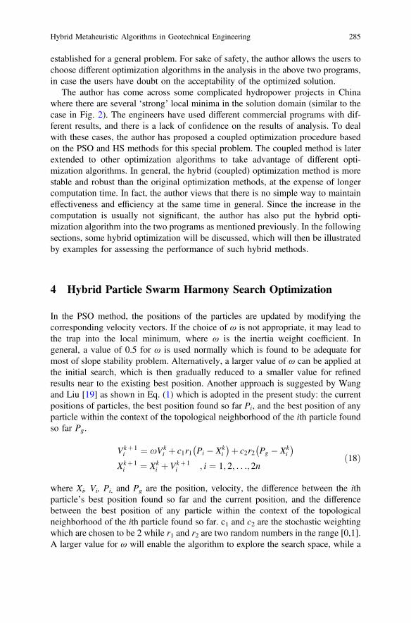
established for a general problem. For sake of safety, the author allows the users tochoose different optimization algorithms in the analysis in the above two programs,in case the users have doubt on the acceptability of the optimized solution.

The author has come across some complicated hydropower projects in Chinawhere there are several ‘strong’ local minima in the solution domain (similar to thecase in Fig. 2). The engineers have used different commercial programs with dif-ferent results, and there is a lack of confidence on the results of analysis. To dealwith these cases, the author has proposed a coupled optimization procedure basedon the PSO and HS methods for this special problem. The coupled method is laterextended to other optimization algorithms to take advantage of different opti-mization algorithms. In general, the hybrid (coupled) optimization method is morestable and robust than the original optimization methods, at the expense of longercomputation time. In fact, the author views that there is no simple way to maintaineffectiveness and efficiency at the same time in general. Since the increase in thecomputation is usually not significant, the author has also put the hybrid opti-mization algorithm into the two programs as mentioned previously. In the followingsections, some hybrid optimization will be discussed, which will then be illustratedby examples for assessing the performance of such hybrid methods.

4 Hybrid Particle Swarm Harmony Search Optimization

In the PSO method, the positions of the particles are updated by modifying thecorresponding velocity vectors. If the choice of ω is not appropriate, it may lead tothe trap into the local minimum, where ω is the inertia weight coefficient. Ingeneral, a value of 0.5 for ω is used normally which is found to be adequate formost of slope stability problem. Alternatively, a larger value of ω can be applied atthe initial search, which is then gradually reduced to a smaller value for refinedresults near to the existing best position. Another approach is suggested by Wangand Liu [19] as shown in Eq. (1) which is adopted in the present study: the currentpositions of particles, the best position found so far Pi, and the best position of anyparticle within the context of the topological neighborhood of the ith particle foundso far Pg.

Vkþ 1i ¼ xVk

i þ c1r1 Pi � Xki

� �þ c2r2 Pg � Xki

� �

Xkþ 1i ¼ Xk

i þVkþ 1i ; i ¼ 1; 2; . . .; 2n

ð18Þ

where Xi, Vi, Pi, and Pg are the position, velocity, the difference between the ithparticle’s best position found so far and the current position, and the differencebetween the best position of any particle within the context of the topologicalneighborhood of the ith particle found so far. c1 and c2 are the stochastic weightingwhich are chosen to be 2 while r1 and r2 are two random numbers in the range [0,1].A larger value for ω will enable the algorithm to explore the search space, while a

Hybrid Metaheuristic Algorithms in Geotechnical Engineering 285

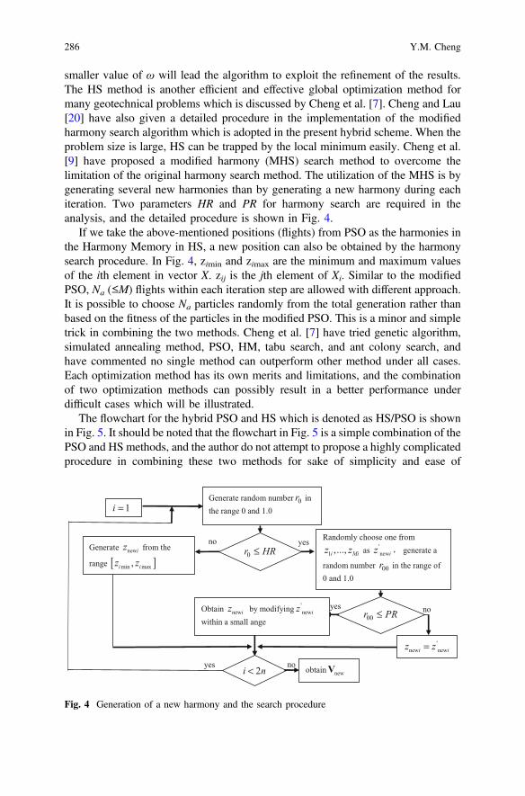
smaller value of ω will lead the algorithm to exploit the refinement of the results.The HS method is another efficient and effective global optimization method formany geotechnical problems which is discussed by Cheng et al. [7]. Cheng and Lau[20] have also given a detailed procedure in the implementation of the modifiedharmony search algorithm which is adopted in the present hybrid scheme. When theproblem size is large, HS can be trapped by the local minimum easily. Cheng et al.[9] have proposed a modified harmony (MHS) search method to overcome thelimitation of the original harmony search method. The utilization of the MHS is bygenerating several new harmonies than by generating a new harmony during eachiteration. Two parameters HR and PR for harmony search are required in theanalysis, and the detailed procedure is shown in Fig. 4.

If we take the above-mentioned positions (flights) from PSO as the harmonies inthe Harmony Memory in HS, a new position can also be obtained by the harmonysearch procedure. In Fig. 4, zimin and zimax are the minimum and maximum valuesof the ith element in vector X. zij is the jth element of Xi. Similar to the modifiedPSO, Na (≤M) flights within each iteration step are allowed with different approach.It is possible to choose Na particles randomly from the total generation rather thanbased on the fitness of the particles in the modified PSO. This is a minor and simpletrick in combining the two methods. Cheng et al. [7] have tried genetic algorithm,simulated annealing method, PSO, HM, tabu search, and ant colony search, andhave commented no single method can outperform other method under all cases.Each optimization method has its own merits and limitations, and the combinationof two optimization methods can possibly result in a better performance underdifficult cases which will be illustrated.

The flowchart for the hybrid PSO and HS which is denoted as HS/PSO is shownin Fig. 5. It should be noted that the flowchart in Fig. 5 is a simple combination of thePSO and HS methods, and the author do not attempt to propose a highly complicatedprocedure in combining these two methods for sake of simplicity and ease of

Fig. 4 Generation of a new harmony and the search procedure

286 Y.M. Cheng

implementation. The step on the updating of the positions of all the particles in thePSO method is replaced by the harmony search generation as given in Fig. 4. Such aminor change can retain the simplicity of both optimization methods so that theproposed algorithm is simple to use and does not require major computer memory.The author has come across several very complicated cases in some projects, and thepresently proposed algorithm combine two optimization methods so that the coupledalgorithm will be more stable and robust for very complicated problem. It is true thatthe present method will be less efficient for simple method and it is not recommendedfor such purposes even though the hybrid method is still effective for such cases. Theproposed algorithm is targeted toward complicated problems (discontinuous objec-tive function with multiple strong local minima and sudden major change in thematerial properties) for which the other algorithms may fail to perform satisfactorily.

Besides the coupling of PSO and HM, it is also possible to couple the tabusearch, simulated annealing, genetic algorithm with the harmony search method,and the author has also successfully implemented these coupling methods.

5 Hybrid Chaos Harmony Search Algorithm (CH/HS)

The chaos phenomenon is first discovered from the simulation of atmosphericturbulence between two infinite planes by the American meteorologist Lorenz in1963. The solution of the equation is not only stochastic but also nonperiodic if

Fig. 5 The flowchart for thehybrid HS/PSO Optimizationmethod

Hybrid Metaheuristic Algorithms in Geotechnical Engineering 287

suitable parameters are selected, which means that a determinate equation couldyield stochastic results. Therefore, it is a kind of behavior between random andrules. However, chaos contains refined internal structure instead of being intricateand disordered, which can confine the systematic motion to a specific scope.Chaotic motion shows strong randomicity, ergodicity, and regularity, and it canchange a lot even if there is only a small change to the initial conditions. Based onthe ergodicity of chaos variables, it is feasible to explore the solution space.

In order to explore the solution space by using chaos variables, the initial valuesshould be obtained first and then the common Logistic Map is adopted to updatethem. Generally, the steps for exploring the chaos are as follows:

• If k = 0, then the initial chaos variable chaosk ¼ chk1; chk2; . . .; ch

km

� �, where m is

the number of designed variable. At the same time, the bounds to the variablesare defined, i.e., U ¼ u1; u2; . . .; umð Þ; L ¼ l1; l2; . . .; lmð Þ, where uj; lj are theupper and lower bounds of the control variable, respectively.

• According to Eq. (19), the chaos variables chaosk can be projected as a point inthe variable space Rk ¼ rk1; r

k2; . . .; r

km

� �as;

rkj ¼ lkj þ ukj � lkj� �

� chkj ; j ¼ 1; 2; . . .;m ð19Þ

• The initial values of the chaos variables are then updated using Eq. (20) beforeturning back to step (2) for continuous iteration, which can find a series ofsolutions, i.e., R0;R1; . . ., and from which the best one can be considered as thesolution of optimization problem

chkþ 1j ¼ chkj � 1� chkj

� �� 4:0; j ¼ 1; 2; . . .;m ð20Þ

It should be noted that the chaos variables have strong ergodicity and can exploresolution space from the preceding steps, but there are also such limitations as badapplication of the optimal solution and poor development capability of the algo-rithm. However, new algorithm with strong global search ability can be developedbased on the combination of harmony algorithm and advanced exploring ability ofchaos algorithm. The author proposes three chaos exploration strategies forresearch, namely simple chaos exploration strategy (SCHM), static partitioningchaos exploration strategy (SPCHM), and dynamic partitioning chaos explorationstrategy (DPCHM).

• Simple chaos exploration strategy is to keep the variable value interval constantduring the exploration, which is given in Eq. (19), that is,

ukj ¼ uj; lkj ¼ lj; j ¼ 1; 2; . . .;m: ð21Þ

• Static partitioning chaos exploration strategy is to divide the user’s givenvariable value interval into several subintervals, and with more subintervals, the

288 Y.M. Cheng

more computational works will be required. Herein, three intervals are selectedas follows:

U1 ¼ u1; u2; . . .; umð Þ; L1 ¼ f1; f2; . . .; fmð ÞU2 ¼ f1; f2; . . .; fmð Þ; L2 ¼ d1; d2; . . .; dmð ÞU3 ¼ d1; d2; . . .; dmð Þ; L3 ¼ l1; l2; . . .; lmð Þ

ð22Þ

where fj ¼ uj � uj�lj3 ; dj ¼ uj � uj�lj

3 � 2; j ¼ 1; 2. . .m. During chaos exploration,three different initial chaos values chaosk;1; chaosk;2; chaosk;3 are formed andthen projected to a series of solutions in U1; L1;U2; L2;U3; L3, respectively. Asfor chaosk;1, it has been reflected in Eq. (19) that ukj ¼ uj; lkj ¼ fj; j ¼ 1; 2; . . .;m.The best solution among the three series is then chosen as the solution of theoptimal problem.

• Dynamic partitioning chaos exploration strategy, namely, solution space isdivided into three subintervals utilizing the worst point in the current harmonylibrary Rb ¼ rb1; rb2; . . .; rbmð Þ, and the center point of the other remained points

Fig. 6 The flowchart of chaos harmony search algorithm

Hybrid Metaheuristic Algorithms in Geotechnical Engineering 289

Ro ¼ ro1; ro;2; . . .; rom� �

. The definition of the interval is analogous to thosedepicted above except for small differences in the values of fj; dj. Herein, fj; djare the maximum and minimum among the worst point and the center point,respectively. i.e., fj ¼ max rbj; roj

� �; dj ¼ min rbj; roj

� �.

The flowchart for the hybrid chaos harmony search method is shown in Fig. 6, inwhich Tm denotes the user’s defined maximum number of iteration. Different chaosexploring strategies will give rise to different Chaos Harmony Method. In theprocess of finding local factors of safety, maximization and minimization aresimulated by the fundamental harmony method and Chaos Harmony Method,respectively.

6 Hybrid Genetic Algorithm with Harmony SearchStrategy (GA/HS)

It is also possible to couple the genetic algorithm, harmony search, simulatedannealing algorithm, tabu search and other methods easily by simple fine tuning inthe generation of new trials. In this section, another hybrid method will be dis-cussed, but the author will not try to discuss any more hybrid methods in thischapter. The main reason is that most of the hybrid methods can perform better thanthe simple methods, but again no single hybrid method seems to outperform otherhybrid methods under all cases, in terms of effectiveness and efficiency. Before thediscussion on the hybrid genetic harmony search, the two basic methods areexplained in more details before the hybrid method can be discussed.

6.1 Harmony Search Algorithm

In music playing, musicians repeatedly adjust the tone of the instrument in the band(based on memory) so as to eventually reach a wonderful state of harmony. TheHarmony Search Algorithm is proposed by Geem based on the inspiration ofconsidering instrument i (i = 1, 2, …, m) and harmony of the instrument tone Rj

(j = 1,2, … s) analogous to the ith design variable and jth solution vector in theoptimization problem. It has been successfully adopted in the combinational opti-mization problems such as slope stability problem, TSP, pipe laying and publictransport line, experimental parameter estimation and others. In this algorithm,M initial solutions (i.e., harmony) are obtained first and put into the HarmonyMemory. It will then search new solutions in HM with a probability of HR whilesearching outside HM with a probability of 1-HR. Thereafter, local disturbance willbe added to the new solutions with a probability of PR. If the objective functionvalue of the new solution is better than the worst solution in HM, then replace it.Iteration will not stop until reaching the maximum evolution generation Tmax and

290 Y.M. Cheng

the computational process is shown in Fig. 7. Fundamental harmony algorithm usedin this chapter adopts punishment and repair strategies to process nonfeasiblesolutions. From Fig. 7, it can be seen that harmony search algorithm belongs tosingle individual evolution algorithm. Although the harmony library is used to yieldnew solutions, only one solution can be found in each evolution. As the approach toform new solutions is very novel, it can be applied in other group evolutionalgorithms, for example, genetic algorithm, to enhance the probability to find newsolutions during the search, and such newly combined algorithm will be of higherglobal search ability.

Fig. 7 The flowchart of fundamental harmony search algorithm

Hybrid Metaheuristic Algorithms in Geotechnical Engineering 291

6.2 Genetic Algorithm

Genetic algorithm is an adaptive global optimization algorithm based on Darwin’stheory of evolution and Mendel’s genetic theory, which was first proposed by J.H.Holland. It is mainly implemented by three operators: selection, hybridization, andmutation. Taking the critical slip surface search of soil slope as an example, theprincipal procedures of genetic algorithm are as follows:

• Determine the design vector of the optimization problem, for example, X ¼xA; xB; . . .; yn�1ð Þ ¼ z1; z2; . . .; znþ 1ð Þ in Eq. (23), and objective function valueG controlled by design vector (i.e., chromosome) X. Regarding to the opti-mization problem of finding the minimum value of objective function, if G issmaller, then corresponding to which the chromosomeXi ¼ zi1; z

i2; . . .; z

inþ 1

� �(where zij denotes the jth gene of the ith chromosome

j ¼ 1; 2; . . .; nþ 1) will be a better adaptation. Then N chromosomesX1;X2; . . .;XN satisfying constrained conditions are formed randomly and putinto the match pool with crossover probability pc and mutation probability pm.Moreover, evolution generation t ¼ 0 and Tmax denotes the maximum evolutiongeneration.

Min G xA; xB; y1; y2; ::; yn�1ð ÞXLA � xA �XUA ; XLB � xB �XUB; YLi � yi � YUi ; i ¼ 1; 2; ::; n� 1

�ð23Þ

• N=2 pairs of parents chromosomes are formed by randomly selecting twochromosomes out of N in the match pool. For each parent chromosomes,crossover operation can be implemented according to pc. If yes, two offspringsS1; S2 will be obtained by operating arithmetic crossover operator on the parentchromosomes, and then S1; S2 are put into children’s pool.

• Mutation should be operated on each offspring in the children’s pool accordingto pm. If yes, the existed offspring should be substituted by another new off-spring formed by the nonuniform mutation operator.

• Compute the objective function value of N chromosomes in the match pool andK chromosomes in the children’s pool, respectively. Punishment and repairstrategies should be adopted if the chromosome is not feasible.

• The objective function values of N þK chromosomes are considered to be in anascending sort order Gm1 ;Gm2 ; . . .;GmN þK . The probability of choosing mi

chromosome is qmi¼ a 1� að Þi�1; a 2 0 1½ �: N chromosomes are reselected

and put into the match pool according to the probability of being chosen foreach chromosome. Specifically, those chromosomes with smaller objectivefunction values will be much more than the others in the match pool.

• t ¼ tþ 1, if t\Tmax, then turn back to step (2), otherwise, output the optimalchromosome and stop iteration.

292 Y.M. Cheng

From the above, it is clear that the match pool in the fundamental genetic algorithmwill be occupied quickly by several excellent chromosomes if the selection pressureis extremely high, that is, a is too large. Generally, it is quite difficult to generateoffspring through crossover as well as mutation, because the mutation rate is usuallyvery small. On the basis of the approach prompting new solutions in harmonysearch algorithm, the harmony genetic algorithm is thus proposed.

7 Genetic Algorithm with Harmony Strategy

The match pool in the genetic algorithm is considered as the harmony library HM,and it will produce new solutions if probability HR and PR are known. The iterationprocedures of harmony genetic algorithm are as follows:

• Under the given probability HR and PR, N ¼ 2� ðnþ 1Þ initial trialX1;X2; . . .;XN satisfying the constrained conditions are formed randomly andput into the match pool with crossover probability pc and mutation probabilitypm. At evolution generation t ¼ 0, Tmax and Phm denote the maximum evolutiongeneration and harmony probability, respectively.

• N=2 pairs of parents chromosomes are formed by randomly selecting twochromosomes out of N in the match pool. For each parent chromosomes,crossover operation can be implemented according to pc. If yes, two offspringsS1; S2 will be obtained by operating arithmetic crossover operator on the parentchromosomes, and then S1; S2 are put into children’s pool.

• Mutation should be operated on each offspring in the children’s pool accordingto pm. If yes, the existing offspring should be substituted by another new off-spring formed by the nonuniform mutation operator.

• According to the N chromosomes in the match pool, N � Phm new solutionsH1; . . .;HN�Phm are produced utilizing harmony algorithm, and then they are putinto the children’s pool.

• Compute the objective function value of N chromosomes in the match pool andK chromosomes in the children’s pool, respectively. Punishment and repairstrategies should be adopted if the chromosome is not feasible.

• The objective function values of N þK chromosomes are considered to be in anascending order Gm1 ;Gm2 ; . . .;GmN þK . The probability of choosing mi chromo-

some is qmi¼ a 1� að Þi�1; a 2 0 1½ �: Currently, N chromosomes are rese-

lected and put into the match pool according to the probability of being chosenof each chromosome. Specifically, those chromosomes with smaller objectivefunction value will be much more than the others in the match pool.

• t ¼ tþ 1, if t\Tmax, then go back to step (2), otherwise, output the optimalchromosome and stop iteration.

Hybrid Metaheuristic Algorithms in Geotechnical Engineering 293

8 Application of Hybrid Optimization Method

For the large-strain pile driving PDA test results in Fig. 3, the length and diameterof the precast pretensioned concrete pile are 26 m and 450 mm, respectively. TheYoung’s modulus of the concrete pile is back-calculated as 45,250 MPa, based onthe time for the reflected signal to travel to the pile top. From this figure, it isdirectly found that the maximum impact force from the diesel hammer is 4787 kN.Two local peaks are observed besides the first peak which is the measured force dueto direct striking by the hammer. These two local peaks represent the force reflectedfrom the junctions between pile segments at a depth of 12 and 24 m below piletop. Based on the minimization of Eq. (17) using commercial program, the endbearing, skin friction, and static pile capacity are found to be 4103, 1942, and5853 kN, respectively, with a prescribed damping factor of 0.1 s/m and a quake of2.5 mm using signal matching approach 1 (commonly adopted parameters usingmanual trial and error). If completely automatic signal matching method is used(signal matching approach 2 with unconstrained bounds), an even better signalmatching is obtained with a damping factor of 0.5 s/m and a quake of 1.3 mm(which are outside the normal ranges in Hong Kong), and the static pile capacity isestimated to be 5415 kN with some major fluctuation in the skin friction at themiddle of the pile. Multiple solutions in signal matching are commonly encounteredby many engineers, and the major differences between soil parameters and pilecapacities obtained from different set of matching are not uncommon. The staticpile capacity by the CASE analysis (Case damping factor = 0.15) is 5765 kN whilethe pile capacity is found to be 6231 kN from static load test. Based on the coupledoptimization HS/PSO as discussed in this chapter, Eq. (17) is solved by assigningan upper and lower bounds to each variable (quake, damping, soil parameters, skinresistance, and base capacity) based on experience of the engineers, and a static pilecapacity of 5946 kN (different parameters to different segments of pile) is obtained.Since the upper and lower bounds are established by soil mechanics principle andexperience, unrealistic values can be avoided in the signal matching process. Thisapproach possesses the advantages of manual control as well as automatic signalmatching, and has been found to be efficient based on some projects in Hong Kong.Using CH/HS and GA/HS, the optimized results are virtually the same as that bythe HS/PSO. Since there is no sharp change in the soil parameters, the static pilecapacity of 5946 kN can be accepted with confidence, even though this problem hasmany local minima in the solution domain.

For slope stability problem, a problem with a soft band which has been con-sidered by Zolfaghari et al. [14], Cheng et al. [9] and Kahatadeniya et al. [21] isshown in Fig. 8. The soil parameters for this problem are shown in Table 1. It isnoticed that the soil parameters for soil layer 3 are much lower than the other threesoils so that the failure surface will be mainly controlled by this layer of soil at themiddle of the failure surface. For minimization of the factor of safety, the minimumvalue using Spencer method for this problem are 1.50, 1.11, 1.361, and 1.09 by thegenetic algorithm [14], the artificial fish swarm algorithm (AFSA) [9], the ant

294 Y.M. Cheng

colony method [21] and HS/PSO. Again, the result by CH/HS and GA/HS arevirtually the same as that by the HS/PSO, which indicate that the performance ofthese three hybrid optimization method are nearly the same for this problems. Sincethe soft band soil is a strong local minimum but the thickness of this layer isrelatively small, the genetic algorithm and the ant colony method cannot escapefrom the local minimum and fail to provide a good solution for this problem. On theother hand, the artificial fish swarm algorithm and the three hybrid methods in thischapter provide solutions which are nearly the same. In fact, it is difficult to dif-ferentiate precisely the critical slip surfaces from the AFSA, HS/PSO, CH/HS, andGA/HS.

For the second problem as shown in Fig. 9, it is one of the sections for a majorhydropower project in China where there are 17 layers of soil beneath the dam. Thematerial parameters are shown in Table 2. It is noticed that soil layers 7, 8, 11, 12,13, and 16 have very low soil parameters, which means that they are the stronglocal minima which can create problem during optimization search. The nature ofthis problem is actually similar to that as shown in Fig. 2. The stability of thefoundation of the dam is extremely important, as this project is very expensive andthe failure of the dam will cause significant loss of lives and properties. Again,many classical optimization methods fail to work well for this case, as there areseveral layers of soft materials which are strong local minima affecting the directionof search for the global minimum.

10 15 20 25 30 35 4041

43

45

47

49

51 Zolfaghari AFSA/HM-PSO Ant-Colony

Fig. 8 A slope stabilityproblem with a soft band

Table 1 Geotechnicalparameters for the soils inFig. 8 (γ = unit weight of soil,c′ = effective cohesivestrength and ϕ′ = effectiveangle of friction)

Layers c(kN/m3) c′ (kPa) u′ (°)

1 19.0 15.0 20.0

2 19.0 17.0 21.0

3 19.0 5.00 10.0

4 19.0 35.0 28.0

Hybrid Metaheuristic Algorithms in Geotechnical Engineering 295

For the present analysis, the left exit end of the failure surface is searched withinthe domain of x = 260 to 330 m while the right exit end is searched within thedomain of x = 520 to 575 m according to the suggested approach by Cheng [15] andCheng et al. [7]. It is noticed that the failure surfaces based on the MHS and MPSOare close to the original MHS and MPSO methods and they are not shown forclarity. It is also noticed that the failure surfaces from all the optimization methodsare virtually the same at the right-hand side as this is strongly governed by the soil

50

100

150

200

250

300

350

400

620520420320220120 m

m

dam profile

AFSA

PSO

HS/PSO

Fig. 9 Critical slip surfaces by different global optimization methods based on the Spencer’smethod (critical failure surface by MHS and MPSO are not shown for clarity)

Table 2 Geotechnicalparameters for the problem inFig. 9

Layers γ (kN/m3) c′ (kPa) ϕ′ (°)

1 16.00 2000.0 56.31

2 24.00 2000.0 56.31

3 24.00 2000.0 56.31

4 26.00 1000.0 50.20

5 26.00 1400.0 54.50

6 26.00 1000.0 44.70

7 26.00 100.0 19.30

8 26.00 100.0 19.30

9 26.00 1000.0 44.70

10 26.00 1400.0 54.50

11 26.00 100.0 19.30

12 26.00 100.0 19.30

13 26.00 100.0 19.30

14 23.00 130.0 22.30

15 26.00 1400.0 54.50

16 26.00 100.0 19.30

17 26.00 1400.0 54.50

296 Y.M. Cheng

profiles and the geometry of this project. The major differences between the failuresurfaces from different methods of optimization as shown in Fig. 9 are: (1) thestarting point of the critical failure surface from HM/PSO is x = 278.0 while itranges from 320.25 to 320.38 for all the other methods; (2) the exit angle of thefailure surface for HM/PSO method is smaller than all the other methods; (3) allthe optimization methods except for the HM/PSO is more attracted by soil 13 in theanalysis so that the critical failure surfaces are deeper than that by the HM/PSO. InTable 3, it is clear that most of the global optimization methods are not satisfactoryexcept for the AFSA which gives a factor of safety less than 2.0 (but still not goodenough while HM, PSO are actually poor in performance) but requires 394,527trials in the analysis. Actually, when the number of control variable is large, theauthors [8] found that HS can be inefficient and sometimes noneffective. It can beviewed that all the optimization methods are attracted by the presence of the“strong” local minima during the search, except for the hybrid HM/PSO, CH/HS,and GA/HS analyzes which are less affected by the “attraction” of the local minima.Based on the proposed coupling method, the minimum factor of safety is obtainedas 1.65 with the three hybrid optimization methods. It is noticed that the hybridoptimization methods are more stable for problems where there are several “strong”local minima. For the present large-scale construction work, a good result is muchmore important than the time of computation, and the proposed hybrid method hasprovided a good result without excessive computations.

The author has considered another case which is illustrated in Fig. 10. Thecohesive strengths of the three soils in Fig. 10 are 28.5 kPa, 0, and 28.5 kPa,respectively, while the friction angles are 20°, 10°, and 20°, respectively (asmeasured from top to bottom). In this problem, the thickness of soil layer 2 is only0.1 m as compared with the width of the potential slip surface which is about 30 m.This problem is more difficult than the one in Fig. 9 because the thickness of thesoft layer is extremely smaller, and this layer will control the failure. Unless thedomain transformation technique is applied, most of the heuristic optimizationalgorithms will fail to obtain the critical failure surface (shown in Fig. 10) and theminimum factor of safety (0.7603) automatically. For the present problem, theresults of analysis are shown in Table 4. It is noticed that only the hybrid methodcan provide good solutions for the present problem. The special feature of thisproblem is that a very minor change in the location of the trial failure surface canhave a great influence in the factor of safety, and there are many discontinuoussolutions during the optimization process. Unless the thickness of soil layer 2

Table 3 Minimum factors of safety for Fig. 9 based on Spencer method (41 control variables)

Method of globaloptimization

PSO MPSO AFSA MHM HM/PSO CH/HS GA/HS

Min. FOS 2.18 2.15 1.83 1.98 1.65 1.65 1.65

No. of trials 121,124 59,288 394,527 132,098 130,156 123,063 133,238

Min. FOS atevaluation number

99,824 35,460 219,284 98,426 112,342 112,436 120,347

Hybrid Metaheuristic Algorithms in Geotechnical Engineering 297

increases to 0.4 m, the classical heuristic optimization algorithms fail to performsatisfactorily. That means, even if an engineer adopts different basic heuristicoptimization algorithms, he may still fail to obtain the critical solution which is0.7603. It is true that problems similar to that in Fig. 10 are not common, but thereare some similar cases in Hong Kong and other countries.

For the present problem, the author has found that there are many local minimumwithin the solution domain, and the factor of safety is very sensitive to the preciselocation of the trial failure surface. A minor change in the location of the trial failuresurface can give rise to noticeable change in the objective function, and the presentproblem is a typical difficult global optimization problem. For example, if antcolony method is used, a factor of safety 0.903 is obtained with the optimumsolution as shown in Fig. 11. If the harmony search method is used, the factor ofsafety will be 0.899. The critical failure surfaces from these two methods also differ

20 25 30 35 40 45 50 55 60 65 70 75 80

16

18

20

22

24

26

28

30

32

34

36

38

40 Soil 1

Soil 2 Soil 1

Fig. 10 A difficult problem illustrating the performance of various optimization algorithms, withthe critical failure surface as shown

Table 4 Minimum factor ofsafety for different methodswithout using the domaintransformation technique byCheng [5]

Method Min. FS

SA 0.8993

HS 0.9453

MHS 0.805

PSO 0.864

MPSO 0.903

GA 0.979

Ant colony 1.068

HS/PSO 0.770

CH/HS 0.765

GA/HS 0.766

298 Y.M. Cheng

noticeably from the critical solution by the hybrid optimization method as shown inFig. 10. It is of course possible to tune the parameters of the various simpleoptimization methods to give the results in Fig. 10, but such tuning is not possibleunless the critical solution is known. If the thickness of the soft band is reduced to0.1 mm, which is equivalent to a very sharp change in the soil parameters within avery narrow region, then no optimization method can give the results in Fig. 10unless the domain transformation technique or equivalently a random function withmore weighting for the soft band zone is used. This case can also illustrate the

20 25 30 35 40 45 50 55 60 65 70 75 80

16

18

20

22

24

26

28

30

32

34

36

38

40 Soil 1

Soil 2 Soil 1

Fig. 11 A local minimum is obtained by the ant colony method for the problem in Fig. 10

20 25 30 35 40 45 50 55 60 65 70 75 80

16

18

20

22

24

26

28

30

32

34

36

38

40 Soil 1

Soil 2 Soil 1

Fig. 12 Another local minimum obtained by the harmony search method for the problem inFig. 10

Hybrid Metaheuristic Algorithms in Geotechnical Engineering 299

limitations of all the heuristic optimization methods that they may not be able tofunction well if there is an extremely sharp change within a very narrow region. Thelimitations of the heuristic or other type of optimization methods should always beaware of during application, and it is well known that there is no universal methodwhich can solve all optimization problems under all conditions (Figs. 12 and 13).

9 Discussion and Conclusion

Many geotechnical and other engineering problem can be formulated as an opti-mization problem, for example, the stability-type problems. There are also manyengineering problems which are governed by partial differential equations but canalso be formulated as the extremum of a functional. Although many classicalproblems can be solved by the use of simplex or gradient methods, there are alsomany types of problems for which many local minima exist in the solution domain.Currently, many researchers are now turning to the use of heuristic optimizationmethods, which are not limited by the presence of a local minimum during theoptimization process.

The author has carried out many studies toward the use of various heuristicoptimization methods in geotechnical problems, and it is established that no singleheuristic global optimization problem can outperform other methods under allcases. Furthermore, it is difficult to design a set of parameters which are suitable forall types of conditions. Every method has its own merits and limitations, and evenautomatic tuning of the parameters may only be suitable for some types of prob-lems. For very complicated problems, particularly for those discontinuous problem

20 25 30 35 40 45 50 55 60 65 70 75 80

16

18

20

22

24

26

28

30

32

34

36

38

40 Soil 1

Soil 2 Soil 1

Fig. 13 All optimization methods fail to obtain the critical solution for a soft band thickness of0.1 mm

300 Y.M. Cheng

or problems with several strong local minima, many simple heuristic optimizationmethods may sometimes fail to give the best solution. In views of that, the authorhas tried to combine the use of two heuristic optimization methods to give a morestable and better performance method with less dependence on the choice ofparameters. The hybrid methods of PSO/HS, CH/HS, and GA/HS as proposed inthis chapter have taken the advantages of two optimization methods so as to give amore stable global optimization. As demonstrated in the present chapter, the hybridmethod can perform better than the simple heuristic optimization methods forcomplicated problems where there are many strong local minima and discontinuousobjective functions. From many practical applications, the author has also noticedthat the increase in the computations as compared with the simple heuristic opti-mization methods is not major. It is true that the hybrid method is less efficient (stilleffective) for many simple problems and is not recommended for such cases. Forthose difficult problems where there are many local minima, the use of the hybridmethods are however more effective at the expense of minor increase in the amountof computations. The author views that effectiveness and efficiency cannot bemaintained simultaneously for arbitrary problems. The proposed hybrid methodsare simple enough to be adopted while the performance is more stable than thesimple methods for the difficult problems. Finally, the author would also like toaddress that every method may fail to work under some very special case, and suchspecial case is usually obvious so that the engineers can adopt some special trick(for example, the domain transformation method by Cheng [5]) to overcome thevery special constraints. Engineers should not rely completely on the optimizationmethods without an evaluation about the nature of the problem.

Acknowledgments The author would like to thanks the Hong Kong Polytechnic University forthe support of present work through project account YBBY.

References

1. Zienkiewicz O.C., Taylor R.L., Zhu J.Z.: The Finite Element Method: its Basis andFundamental, 6th edn. Elsevier, New Work (2005)

2. Denn M.M.: Optimization by Variational Methods. Hills Publishing3. Cheng, Y.M., Li, L., Fang, S.S.: Improved harmony search methods to replace variational

principle in geotechnical problems. J. Mech. 27(1), 107–119 (2011)4. Cheng, Y.M., Li, D.Z., Li, N., Li, Y.Y., Au, S.K.: Solution of some engineering partial

differential equations governed by the minimal of a functional by global optimization method.J. Mech. 29(3), 493–506 (2013)

5. Cheng, Y.M.: Global optimization analysis of slope stability by simulated annealing withdynamic bounds and Dirac function. Eng. Optim. 39(1), 17–32 (2007)

6. Cheng, Y.M., Li, L.: Particle swarm optimization algorithm for non-circular failure surface intwo dimensional slope stability analysis. Comput Geotech. 34(2), 92–103 (2007)

7. Cheng, Y.M., Li, L., Chi, S.C.: Studies on six heuristic global optimization methods in thelocation of critical slip surface for soil slopes. Comput. Geotech. 34, 462–484 (2007)

Hybrid Metaheuristic Algorithms in Geotechnical Engineering 301

8. Cheng, Y.M., Li, L., Chi, S.C., Wei, W.B.: Determination of critical slip surface usingartificial fish swarms algorithm. J. Geotech. Geoenvironmental Eng. ASCE 134(2), 244–251(2008)

9. Cheng, Y.M., Li, L., Lansivaara, T., Chi, S.C., Sun, Y.J.: Minimization of factor of safetyusing different slip surface generation methods and an improved harmony search minimizationalgorithm. Eng. Optim. 40(2), 95–115 (2008)

10. Fleming, K., Weltman, A., Randolph, M., Elson, K.: Piling Engineering, 3rd edn. Taylors andFrancis (2009)

11. Rausche, F., Likins, G. E., Liang, L., Hussein, M.H.: Static and Dynamic Models forCAPWAP Signal Matching. The Art of Foundation Engineering Practice. In: Hussein, M.H.,Anderson, J.B., Camp W.M. (eds.), American Society of Civil Engineers, Reston, pp. 534–553. Geotechnical Special Publication No. 198, VA (2010)

12. Greco, V.R.: Efficient monte carlo technique for locating critical slip surface. J. Geotech. Eng.ASCE 122, 517–525 (1996)

13. Malkawi, A.I.H., Hassan, W.F., Sarma, S.K.: Global search method for locating general slipsurface using Monte Carlo techniques. J. Geotech. Geoenvironmental Eng. 127, 688–698(2001)

14. Zolfaghari, A.R., Heath, A.C., McCombie, P.F.: Simple genetic algorithm search for criticalnon-circular failure surface in slope stability analysis. Comput. Geotech. 32, 139–152 (2005)

15. Cheng, Y.M.: Locations of critical failure surface and some further studies on slope stabilityanalysis. Comput. Geotech. 30, 255–267 (2003)

16. Cheng, Y.M., Li, N. (2010), A coupled global optimization algorithm for difficult problems,The young Southeast Asian Geotechnical Conference, Taipei, Taiwan, May 9–12, p. 22

17. Cheng, Y.M., Li, L., Sun, Y.J., Au, S.K.: A coupled particle swarm and harmony searchoptimization algorithm for difficult geotechnical problems. Struct. Multi. Optim. 45, 489–501(2012)

18. Cheng, Y.M., Lansivaara, T., Baker, R., Li, N.: The use of internal and external variables andextremum principle in limit equilibrium formulations with application to bearing capacity andslope stability problems. Soils Found. 53(1), 130–143 (2013)

19. Wang, L., Liu, B.: Particle Swarm Optimization and Scheduling Algorithms. TsinghuaUniversity Press, China (2008)

20. Cheng, Y.M., Lau, C.K.: Soil Slope Stability Analysis and Stabilization—New Methods andInsights, 2nd edn. Spon Press, (2014)

21. Kahatadeniya, K.S., Nanakorn, P., Neaupane, K.M.: Determination of the critical failuresurface for slope stability analysis using ant colony optimization. Eng. Geol. 108, 133–141(2009)

302 Y.M. Cheng