Embed Size (px)
Citation preview

POLITECHNIKA KOSZALIŃSKA
Zeszyty Naukowe
Wydziału Elektroniki i Informatyki
Nr 8
KOSZALIN 2015

Zeszyty Naukowe Wydziału Elektroniki i Informatyki Nr 8
ISSN 1897-7421 ISBN 978-83-7365-402-0
Przewodniczący Uczelnianej Rady Wydawniczej
Mirosław Maliński
Przewodniczący Komitetu Redakcyjnego Aleksy Patryn
Komitet Redakcyjny Mirosław Maliński
Volodymyr Khadzhynov
Adam Słowik
Wiesław Madej
Józef Drabarek
Projekt okładki Tadeusz Walczak
Skład, łamanie Maciej Bączek
© Copyright by Wydawnictwo Uczelniane Politechniki Koszalińskiej Koszalin 2015
Wydawnictwo Uczelniane Politechniki Koszalińskiej 75-620 Koszalin, ul. Racławicka 15-17
Koszalin 2015, wyd. I, ark. wyd. 5,87, format B-5, nakład 100 egz. Druk: INTRO-DRUK, Koszalin

Spis treści
Bohdan Andriyevsky, Vasyl’ Kurlyak, Vasyl’ Stadnyk ............................................................................................ 5
Electronic-and-optical properties of Rb2ZnCl4 crystals
Bohdan Andriyevsky, Klaus Doll, Timo Jacob .................................................................................................................. 15
Electronic band structure and migration of lithium ions in LiCoO2
Dariusz Jacek Jakóbczak ............................................................................................................................................................................... 25
Data Forecasting and Extrapolation via Probability Distribution and Nodes
Combination
Marcin Walczak .......................................................................................................................................................................................................... 39
Modified small-signal models of BUCK, BOOST and BUCK-BOOST DC-DC
converters
Natalija Maslennikowa, Anatolij Sergiyenko....................................................................................................................... 53
Scheduling of synchronous dataflow graphs for datapath synthesis
A.K. Fedotov, I.L. Baranov, M.V. Malashchonak, E.A. Streltsov, I.A. Svito,
A.V. Mazanik .................................................................................................................................................................................................................. 61
Magnetoresistive properties of Ni/TiO2/Ti and Ni/SiO2/Si structures: comparative
analysis
Igor Troyanchuk, Maxim Bushinsky, Nina Tereshko, Vera Fedotova .................................................... 69
Magnetic and magnetotransport properties of La0.5Sr0.5Co0.8Me0.2O3 (Me=Cr, Fe)
cobaltites
Katarzyna Peplińska-Matysiak, Sebastian Pecolt ........................................................................................................... 77
System akwizycji danych na bazie platformy Arduino
Mariusz Miziołek ……............................................................................................................................................................................................ 85
Algorytm i implementacja protokołu komunikacyjnego MODBUS w środowisku
sterownika PLC firmy IDEC oraz języku programowania C#
Valery Susłow, Michał Statkiewicz, Jacek Kowalczyk, Marta Boińska, Janina Nowak ... 97
Cechy osobowości studentów informatyki w kontekście gotowości zawodowej

Bohdan Andriyevsky Chair of Foundations of Electronics Faculty of Electronics and Computer Sciences Koszalin University of Technology, Poland Vasyl’ Kurlyak Mykola Romanyuk Volodymyr Stakhura Chair of Experimental Physics Faculty of Physics I. Franko National University of L'viv, Ukraine Vasyl’ Stadnyk Chair of Solid State Physics Faculty of Physics I. Franko National University of L'viv, Ukraine
Electronic-and-optical properties of Rb2ZnCl 4 crystals
1. Introduction The crystals of dirubidium tetrachlorozincate, Rb2ZnCl4, are a typical example
of the incommensuratelly modulated structures A2BX4. They experience the standard for these crystals sequence of phase transitions (PT): paraelectric phase (Ti = 302 K) → incommensurate phase (TC = 192 K) → commensurate phase [1 - 3]. The high temperature phase I of the crystal is paraelectric with the space group of symmetry Pnam (no. 62) and the corresponding unit cell contains four formula units, Z = 4. The intermediate phase II (TC < T < Ti) is incommensurately modulated in the a-direction of unit cell with the wave vector q = (1 - δ)a*/3. The low temperature phase III (Pna21, q = a*/3) is improper ferroelectric one with the spontaneous polarization vector along c-axis and triple unit cell dimension along a-axis. At the temperature 74 K, the crystal undergoes phase transition into the monoclinic structure of C1c1 space group of symmetry, which in fact is doubled related to the structure of Pna21 along b-axis and contains 48 formula units [3, 4].
The incommensurate phase of Rb2ZnCl4 has been studied by the method of electron diffraction. Below Ti, additional blurred spots appear on the diffraction
B. Andriyevsky, V. Kurlyak, V. Stadnyk, M. Romanyuk, V. Stakhura 6
pattern, which are responsible for appearance the incommensurate phase in the crystal with additional modulation in a-direction [5, 6].
Previously, temperature dependencies of the birefringence δ(Δni) of Rb2ZnCl4 for only one wavelength have indicated that deviation from the linear dependency δ(Δni) = k⋅T in the paraelectric phase are observed at decreasing temperature long before Ti [7 - 9]. The linear electro-optic effect is not observed in the incommensurate phase of the crystal because macroscopically this phase remains center symmetrical [9, 10].
In spite of the considerable interest, complex study of the refractive properties of Rb2ZnCl4 in wide spectral and temperature ranges is not jet done. The probable influence of the uniaxial mechanical stresses on the refractive properties and he temperatures TC and Ti of the crystal are also not studied. Previously, considerable uniaxial baric sensitivity of the refractive index and birefringence had been indicated for the isomorphic K2ZnCl4 crystal [11, 12]. We do not know any theoretical ab initio reference study on the electronic band structure and optical properties of Rb2ZnCl4.
In the present study, theoretical results of first principles calculations of electronic and optical properties and experimental results of refractive properties of the mechanically free and uniaxially stresses Rb2ZnCl4 crystal are presented.
2. Methods of investigations Calculations of the electronic structure and optical properties of Rb2ZnCl4 have
been performed by the CASTEP program [13], based on the density functional theory (DFT) and plane-waves, with using the ultrasoft pseudopotentials [14]. The generalized gradient approximation (GGA) for the exchange and correlation effects [15] and the cutoff energy 340 eV for the plane-waves basis set were used. The electronic eigen-energy convergence tolerance was chosen to be 2.4⋅10-7 eV and the tolerance for the electronic total energy convergence during crystal structure optimization was 1⋅10-5 eV. Also, the corresponding maximum ionic force tolerance was 3·10-2 eV/Å and the maximum stress component tolerance was taken to be 5·10-
2 GPa. Optimization (relaxation) of the atomic positions and crystal’s unit cell parameters at every value of the external stress was performed before the calculations of the electronic characteristic: total electronic energy E, band energy dispersion E(K), partial density of electronic states (PDOS), and dielectric functions ε(hω). Band structure of the crystal was calculated for 34 K-points of the Brillouin zone (BZ) at the space group of symmetry no. 62. The calculations were performed using the semi-empirical dispersion interaction correction module taking into account the van-der-Waals interactions between atoms [16].

Electronic-and-optical properties of Rb2ZnCl4 crystals 7
Single crystals Rb2ZnCl4 were grown from water solutions using the method of slow cooling. The grown crystals had a form of the rhombic prisms with a lot of facets. Experimental measurements of refractive indices ni and its changes under uniaxial mechanical stress σm were performed using the method described in [17]. Analysis of baric changes of the principal refractive indices ni of the crystal was performed using the following definition of the piezo-and-optical coefficient πim [18],
6,...,2,1,, == mia mimi σπδ , (1)
where
33
21
i
i
ii n
n
na
δδδ −=
= . (2)
3. Results and discussion The refractive index dispersion ni(λ) of Rb2ZnCl4 crystal have been measured in
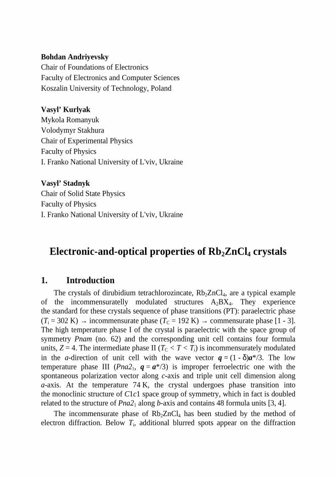
the wavelength range λ 270 nm to 750 nm for different light polarizations (i = x, y, z) and uniaxial stresses at ambient temperature (Fig. 1). In this spectral range, the dispersion of mechanically free and stressed samples is normal (dni/dλ < 0) and its absolute value increases rapidly when the wavelength reaches the long wavelength edge of fundamental absorption of the crystal. It is also seen from figure 1 that the uniaxial stresses do not change the character of the curves ni(λ), but change only the dispersion magnitude dni/dλ (dna/dλ = 12,7⋅10-5 and 12,0⋅10-5, dnb/dλ = 11,2⋅10-5 and 10,6⋅10-5, and dnc/dλ = 12,1⋅10-5 and 11,8⋅10-5 in the wavelength region near λ = 500 nm for the mechanically free and uniaxially stressed samples by the pressure σz = 200 bar, respectively).
B. Andriyevsky, V. Kurlyak, V. Stadnyk, M. Romanyuk, V. Stakhura 8
Figure 1. Refractive index dispersion curves of Rb2ZnCL4 crystal at ambient temperature and external compression 200 bar (0.02 GPa) (i = b, c – crystallographic axes, ο - mechanically free sample, - compression along b-axis, - compression along c-axis, ∑ - compression along a-axis)
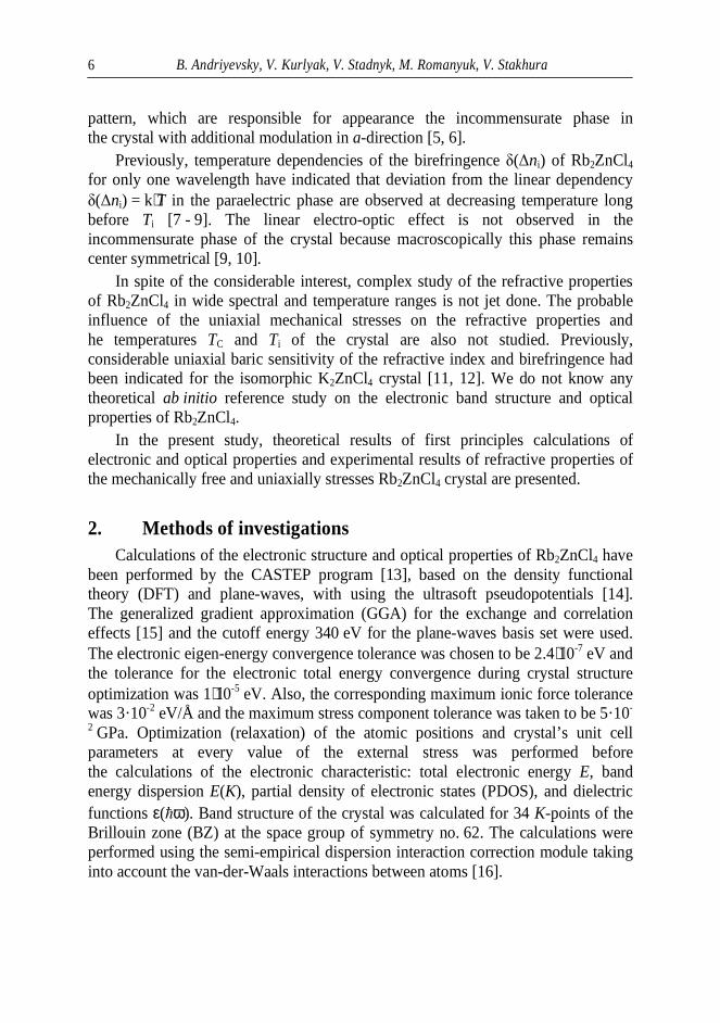
Figure 2. Baric dependencies of principal refractive indices ni (λ = 500 nm) of Rb2ZnCL4 crystal at ambient temperature (i = a, b, c – crystallographic axes, - compression along c-axis, - compression along b-axis, - compression along a-axis)
400 600 800
1.56
1.59
1.62n i
cb
λ /nm
0 50 100 150 200
1.569
1.570
1.576
1.578
1.580
1.582
1.584
c
b
σ /bar
n i
a

Electronic-and-optical properties of Rb2ZnCl4 crystals 9
The averaged specific increase of refractive indices caused by the uniaxial compression is found to be near dni/dσ ≈ 2⋅10-6 bar-1 (Fig. 2).
Band structures and dielectric functions ε(hω) of Rb2ZnCl4 have been calculated for the space groups no. 62. The total energy Et of the crystal is equal to -18685.755 eV (without dispersion corrections) and -18691.574 eV (with dispersion corrections). So, the difference ∆Et = 5.82 eV may be regarded as a characteristic parameter of the van-der-Waals interaction in Rb2ZnCl4.
The calculated energy band gap of the crystal is found to be Eg= 4.47 eV (Γ - Γ), that is expected to be approximately 1 eV to 2 eV smaller than corresponding experimental value, because of the known features of the local density approximation of DFT [19]. This band gap Eg corresponds to the Γ - Γ transition of the Brillouin zone.
Analysis of Rb2ZnCl4 partial density of states have revealed that highest valence bands of the crystal are formed mainly by the p-states of oxygen and lowest conduction bands originate from the s-states of rubidium and zinc. Energy positions of the valence bands partial density of states maxima of Rb2ZnCl4 are found to be very similar to those for K2ZnCl4 crystals obtained by using the ab initio VASP code [20]. The only differences concern to the PDOS of potassium in K2ZnCl4 and rubidium in Rb2ZnCl4. Results of our calculation are in moderate agreement with the photoelectron spectra of Rb2ZnCl4 [21].
We have calculated also the elastic coefficients of Rb2ZnCl4 (space group no. 62) on the basis of the relaxed structure of the crystal (Table 1), which may be compared with the experimental data [22]. These data may be useful for the analysis of piezo-optical properties of the crystal.
Table 1. Elastic modulus B and coefficients of elastic stiffness cij (i, j = 1, 2, ... 6) of Rb2ZnCl4 calculated at space groups no. 62 (a = 9.33 Å, b = 12.6 Å, c = 7.10 Å, V = 835 Å3). All values are in GPa units.
B c11 c22 c33 c12 c13 c23 c44 c55 c66
no. 62 15 38 22 33 8 11 8 7 11 7
Optical functions of crystals originated from the electronic excitations are calculated in CASTEP on the basis of the wave functions Ψ and band structure energies E. The imaginary part of the dielectric function ε2(hω) is obtained from the following relation [23],
( ) ( )2
2
2, ,0
2ˆε δ
ε
c v c v
v c
eE E
V
πω ω= ⟨Ψ ⋅ Ψ ⟩ − −∑h hK K K KK
u r
(3)
B. Andriyevsky, V. Kurlyak, V. Stadnyk, M. Romanyuk, V. Stakhura 10
and then the corresponding real part ε1(hω) is calculated using the following Kramers-Kronig equation.
( )2
1 220
2 ε ( )ε ( ) 1
t t dt
tω
π ω
∞
− =−∫h
h
(4)
The indices of absorption (k) and refraction (n) are connected with the real (ε1) and imaginary (ε2) parts of the complex dielectric function of a material according to the know relations: ε1 = n2 - k2, ε2 = 2nk.
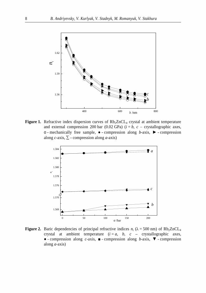
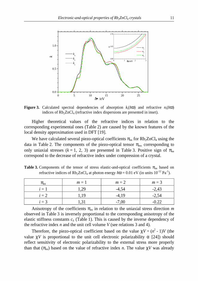
The calculated optical properties of Rb2ZnCl4 are presented in figure 3. The calculated spectra of absorption index k(hω) of Rb2ZnCl4 (Fig. 3) are in moderate agreement with the experimental reflectance spectra of the crystal obtained in the photon energy range 0 eV to 35 eV with using the synchrotron radiation [21]. Position of the main maximum of the calculated spectrum k(hω) at hω = 10 eV agrees well with magnitude of the corresponding experimental maximum of the reflection spectrum R(hω). Large difference of our calculated spectrum k(hω) and experimental one R(hω) in the range hω < 8 eV is explained by the excitonic effects occurred in this spectral range, which are not taken into account in the DFT-based calculations of optical properties using CASTEP code. Also, the calculated energy band gap Eg of the crystal (Eg ≈ 4.5 eV) is much smaller than the corresponding value Eg ≈ 8.0 eV estimated in the reference [21] on the basis of analysis of the excitonic structure of Rb2ZnCl4 with two maxima located in the energy range 7.0 eV to 8.0 eV. Besides, the underestimated value of the calculated band gap Eg of Rb2ZnCl4 was expected because of the known features of the DFT local density approximation.
Experimental and calculated refractive indices of Rb2ZnCl4 are presented in Table 2.
Table 2. Refractive indices nx. ny. and nz of Rb2ZnCl4: experimental (at photon energy hω = 1.68 eV) and calculated (at photon energy hω = 0.01 eV) for mechanically free (σ = 0) and uniaxially stressed crystal (σx = σy = σz = 1 GPa).
Experimental Theoretical σ = 0 σx σy σz
nx 1.5660 1.6429 1.6401 1.6530 1.6483 ny 1.5525 1.6240 1.6215 1.6330 1.6295 nz 1.5564 1.6292 1.6264 1.6444 1.6297
Electronic-and-optical properties of Rb2ZnCl4 crystals 11
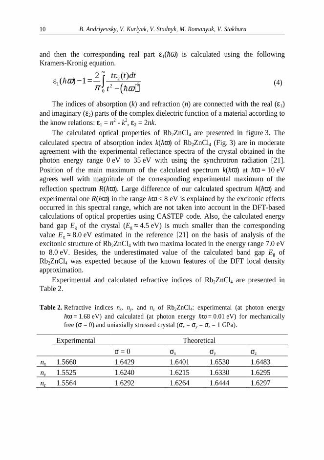
Figure 3. Calculated spectral dependencies of absorption ki(hω) and refractive ni(hω) indices of Rb2ZnCl4 (refractive index dispersions are presented in inset).
Higher theoretical values of the refractive indices in relation to the corresponding experimental ones (Table 2) are caused by the known features of the local density approximation used in DFT [19].
We have calculated several piezo-optical coefficients πim for Rb2ZnCl4 using the data in Table 2. The components of the piezo-optical tensor πim, corresponding to only uniaxial stresses (k = 1, 2, 3) are presented in Table 3. Positive sign of πim correspond to the decrease of refractive index under compression of a crystal.
Table 3. Components of the tensor of stress elastic-and-optical coefficients πim based on refractive indices of Rb2ZnCl4 at photon energy hω = 0.01 eV (in units 10-12 Pa-1).
πim m = 1 m = 2 m = 3
i = 1 1,29 -4,54 -2,43 i = 2 1,19 -4,19 -2,54 i = 3 1,31 -7,00 -0.22
Anisotropy of the coefficients πim in relation to the uniaxial stress direction m observed in Table 3 is inversely proportional to the corresponding anisotropy of the elastic stiffness constants cii (Table 1). This is caused by the inverse dependency of the refractive index n and the unit cell volume V (see relations 3 and 4).
Therefore, the piezo-optical coefficient based on the value χV = (n2 - 1)V (the value χV is proportional to the unit cell electronic polarizability α [24]) should reflect sensitivity of electronic polarizability to the external stress more properly than that (πim) based on the value of refractive index n. The value χV was already
0 5 10 15 20 250.0
0.5
1.0
0 1 2 31.60
1.65
1.70
nx
ny
nz
n
hω /eV
kx
ky
kz
k
h /eV

B. Andriyevsky, V. Kurlyak, V. Stadnyk, M. Romanyuk, V. Stakhura 12
used for the study of influence of the uniaxial stresses on the optical properties of K2SO4 crystals [20].
Table 4. Components of the tensor χiiV (i = 1, 2, 3) (at photon energy hω = 0.01 eV) for relaxed (σ = 0) and mechanically stressed (σii = 1 GPa) Rb2ZnCl4 crystal (χavV is an averaged component) and corresponding band gap Eg. The relative changes are indicated in brackets.
χiiV Stress
χ11V Å3
χ22V Å3
χ33V Å3
χavV Å3
Eg eV
σ = 0 1419 1367 1381 1389 4.467
σ11 1403
(-0.011) 1352
(-0.011) 1365
(-0.012) 1373
(-0.011) 4.542
(0.017)
σ22 1412
(-0.005) 1358
(-0.007) 1388
(0.005) 1386
(-0.002) 4.550
(0.019)
σ33 1416
(-0.002) 1365
(-0.001) 1366
(-0.011) 1382
(-0.005) 4.296
(-0.038)
The relative changes δ(χiiV)/χiiV of the value χiiV under an influence of the uniaxial compression of 1 GPa on Rb2ZnCl4 do not exceed the range -1.2% to 0.5% (Table 4), that means rather small corresponding changes of the electronic polarizability of the crystal. The relative averaged changes δ(χavV)/χavV was found to be negative for all three principal directions of the uniaxial compression (Table 4). It is remarkable that absolute values |δ(χavV)/χavV|ii correlate with corresponding refractive indices nii and unit cell electronic polarizabilities χiiV of the relaxed Rb2ZnCl4 crystal. On the other hand side, baric changes of the energy band gap Eg look uncorrelated with the corresponding changes of refractive indices (n) and unit cell polarizability (χV).
4. Conclusions Partial density of states of Rb2ZnCl4 are found to be very similar to those
obtained earlier for K2ZnCl4 crystals, that indicates for similarity of the electronic structure in two crystals, which in turn is due to the common anion ZnCl4
2-. Changes of the energy band gap Eg of Rb2ZnCl4 under the uniaxial compression
along the principal crystallographic axes i (i = 1, 2, 3) were found to be uncorrelated with the corresponding changes of the refractive indices nii and the unit cell electronic polarizability χiiV of the crystal.
The relative changes of the unit cell electronic polarizability of Rb2ZnCl4 under an influence of the uniaxial compression of 1 GPa do not exceed the values -1.2% to

Electronic-and-optical properties of Rb2ZnCl4 crystals 13
0.5%, that indicates small baric changes of the corresponding electronic polarizability.
Anisotropy of the piezo-optical coefficients πii of Rb2ZnCl4 in relation to the uniaxial stress direction is found to be inversely proportional to the corresponding anisotropy of the elastic stiffness constants cii.
References 1. S. R. Andrews, H. J. Mashiyama. J. Phys. C.: Sol. State Phys. 16 (1983) 4985. 2. M. Quilichini, J. Panetier. Acta Cryst. B 39 (1983) 657. 3. Sh. Hirotsu, K. Toyota, K. Hamano. J. Phys. Soc. Jap. 46 (1979) 1389. 4. H. М. Lu and J. R. Hardy. Phys. Rev. B 45 (1992) 7609. 5. R. Blinc, B. Losar, F. Milia, R. Kind. J. Phys C.: Solid State Phys. 17 (1984)
241. 6. K. Tsuda, N. Yamamoto, K. Yagi. J. Phys. Soc. Jap. 57 (1988) 2057. 7. S.V. Melnikova, А.Т. Аnistratov. Phys. Solid State 25 (1983) 848 (in Russian). 8. P. Gunter, R. Sunctuary, F. Rohner, H. Arend, N. Seidenbusch. Solid State
Commun. 37 (1981) 883. 9. J. Krouрa, J. Fousek. Jap. J. of Appl. Phys. 24 (1985) 787. 10. R. Sunctuary, P. Gunter. Phys. Stat. Solidi (а) 84 (1984) 103. 11. V.Yo. Stadnyk, M. O. Romanyuk , B. V. Andrievsky, Z. O. Kohut. Оptics and
Spectroscopy 108 (2010) 753. 12. M. Gaba, V. Yo. Stadnyk, Z. O. Kohut, R. S. Brezvin. J. Appl. Spectr. 77 (2010)
648. 13. S. J. Clark, M. D. Segall, C. J. Pickard, P. J. Hasnip, M. J. Probert, K. Refson, M.
C. Payne, Zeitschrift fuer Kristallographie 220 (2005) 567. 14. D. Vanderbilt, Phys. Rev. B 41 (1990) 7892. 15. J.P. Perdew, K. Burke, M. Ernzerhof, Phys. Rev. Lett. 77 (1996) 3865. 16. E.R. McNellis, J. Meyer, K. Reuter, Phys. Rev. B 80 (2009) 205414. 17. V.Yo. Stadnyk, M.O. Romanyuk, R.S. Brezvin. Electronic polarizability of
ferroics. L'viv: I. Franko LNU Publ. (2013). 392 pp. (in Ukrainian) 18. T. S. Narasimhamurty Photoelastic and Electro-Optic Properties of Crystals. –
New York and London.: Plenum Press 1981. 514 pp. 19. J. P. Perdew, Int. J. Quantum Chem. 28 (1985) 497. 20. B. Andriyevsky, V. Stadnyk, Z. Kohut, M. Romanyuk, M. Jaskólski,
Mater. Chem. Phys. 124 (2010) 845. 21. A. Ohnishi, M. Saito, M. Kitaura, M. Itoh, M. Sasaki, J. Lumin. 132 (2012)
2639.

B. Andriyevsky, V. Kurlyak, V. Stadnyk, M. Romanyuk, V. Stakhura 14
22. A.V. Kityk, . V.P. Soprunyuk, O.G. Vlokh, Phys. Status Solidi (a) 138 (1993) 119.
23. http://www.tcm.phy.cam.ac.uk/castep/documentation/WebHelp/CASTEP.html. 24. M. Born, E. Wolf, Principles of Optics, Pergamon, Oxford, 1984.
Abstract Electronic-and-optical properties of Rb2ZnCl4 crystal have been studied using
the theoretical and experimental methods. First principles calculations of the electronic structure and optical properties using the density functional theory have been performed on the relaxed and uniaxially compressed (1 GPa) Rb2ZnCl4 crystal. The refractive indices of Rb2ZnCl4 have been measured in the spectral range of wavelength 300 nm to 750 nm for three principal uniaxial compression stresses (0.02 GPa) at room temperature. Ab initio calculations and analysis have revealed that the observed uniaxial pressure changes of the refractive indices of Rb2ZnCl4 are caused mainly by the corresponding changes of the crystal unit cell dimensions. The unit cell electronic polarizability of the crystal remains approximately unchanged.
Streszczenie Zbadano właściwości elektronowo-optyczne kryształów Rb2ZnCl4 metodami
teoretyczną i doświadczalną. Wykonano obliczenia z pierwszych zasad (ab initio) struktury elektronowej i właściwości optycznych na bazie teorii funkcjonału gęstości zrelaksowanych i jednoosiowo ściśniętych (1 GPa) kryształów. Zostały pomierzone współczynniki załamania Rb2ZnCl4 w przedziale długości fal światła 300 nm do 750 nm dla trzech głównych krystalograficznych kierunków ściskania (0.02 GPa) przy temperaturze pokojowej. Obliczenia ab initio i analiza danych ujawniły, że obserwowane baryczne zmiany współczynników załamania Rb2ZnCl4 są spowodowane głównie odpowiednimi zmianami rozmiarów komórki elementarnej kryształu. Przy tym, polaryzowalność elektronowa komórki kryształu pozostaję się prawie niezmienną.

Bohdan Andriyevsky Foundations of Electronics Chair Faculty of Electronics and Computer Sciences Koszalin University of Technology, Poland Klaus Doll Institute of Electrochemistry University of Ulm, Germany Timo Jacob Institute of Electrochemistry University of Ulm, Germany
Electronic band structure and migration of lithium ions in LiCoO2
Key words: electrochemical battery, LiCoO2, electronic band structure, activation energy of lithium ion self-diffusion
Introduction Lithium cobalt oxide LiCoO2 has founded application in rechargeable lithium
ion batteries mainly as a cathode [1, 2]. This material possesses the layered crystal
structure, which has rhombohedral symmetry and belongs to the space group _
3R m. This circumstance is favorable to the accommodation lithium in concentrations, which may change over a relatively large range [3]. Applications of LiCoO2 with deintercalated lithium LixCoO2 (x < 1) as cathode material in solid-state batteries are also taken place widely.
To build adequate mathematical model of the solid-state battery one should take into account numerous phenomena [4, 5]. One of the crucial points of these models is an achievement of the low activation energy for electric transport of solid electrodes and electrolytes. This activation energy depends generally on the electronic structure of the material [6], which may be modified by changing of the chemical elements contained, and external influences. The electronic band structure of LiCoO2 was studied previously by using first principles methods [7 - 15]. The
Bohdan Andriyevskyy, Klaus Doll, Timo Jacob 16
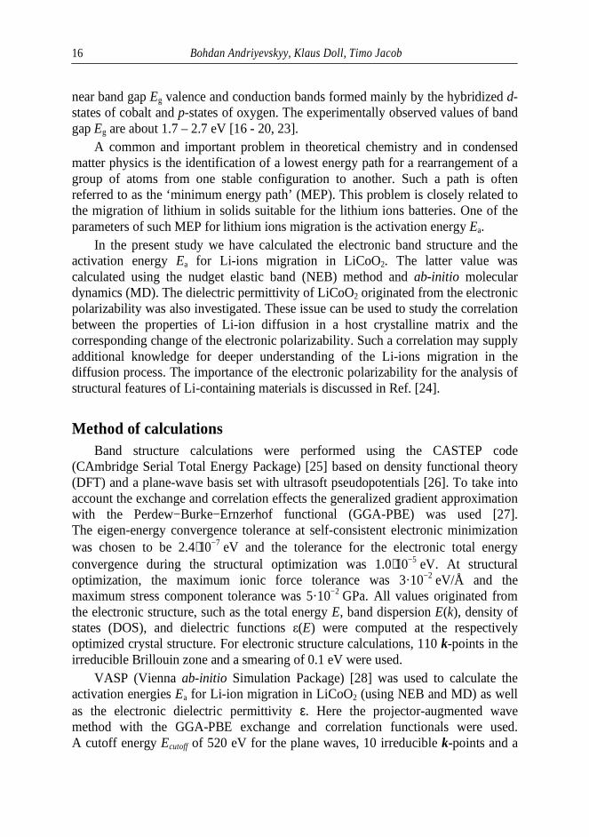
near band gap Eg valence and conduction bands formed mainly by the hybridized d-states of cobalt and p-states of oxygen. The experimentally observed values of band gap Eg are about 1.7 – 2.7 eV [16 - 20, 23].
A common and important problem in theoretical chemistry and in condensed matter physics is the identification of a lowest energy path for a rearrangement of a group of atoms from one stable configuration to another. Such a path is often referred to as the ‘minimum energy path’ (MEP). This problem is closely related to the migration of lithium in solids suitable for the lithium ions batteries. One of the parameters of such MEP for lithium ions migration is the activation energy Ea.
In the present study we have calculated the electronic band structure and the activation energy Ea for Li-ions migration in LiCoO2. The latter value was calculated using the nudget elastic band (NEB) method and ab-initio molecular dynamics (MD). The dielectric permittivity of LiCoO2 originated from the electronic polarizability was also investigated. These issue can be used to study the correlation between the properties of Li-ion diffusion in a host crystalline matrix and the corresponding change of the electronic polarizability. Such a correlation may supply additional knowledge for deeper understanding of the Li-ions migration in the diffusion process. The importance of the electronic polarizability for the analysis of structural features of Li-containing materials is discussed in Ref. [24].
Method of calculations Band structure calculations were performed using the CASTEP code
(CAmbridge Serial Total Energy Package) [25] based on density functional theory (DFT) and a plane-wave basis set with ultrasoft pseudopotentials [26]. To take into account the exchange and correlation effects the generalized gradient approximation with the Perdew−Burke−Ernzerhof functional (GGA-PBE) was used [27]. The eigen-energy convergence tolerance at self-consistent electronic minimization was chosen to be 2.4⋅10−7 eV and the tolerance for the electronic total energy convergence during the structural optimization was 1.0⋅10−5 eV. At structural optimization, the maximum ionic force tolerance was 3·10−2 eV/Å and the maximum stress component tolerance was 5·10−2 GPa. All values originated from the electronic structure, such as the total energy E, band dispersion E(k), density of states (DOS), and dielectric functions ε(E) were computed at the respectively optimized crystal structure. For electronic structure calculations, 110 k-points in the irreducible Brillouin zone and a smearing of 0.1 eV were used.
VASP (Vienna ab-initio Simulation Package) [28] was used to calculate the activation energies Ea for Li-ion migration in LiCoO2 (using NEB and MD) as well as the electronic dielectric permittivity ε. Here the projector-augmented wave method with the GGA-PBE exchange and correlation functionals were used. A cutoff energy Ecutoff of 520 eV for the plane waves, 10 irreducible k-points and a
Electronic band structure and migration of lithium ions in LiCoO2 17
smearing of 0.2 eV were used for the calculations on the crystal supercell of the size 2×2×1 (the volume of the supercell corresponds to Vsc = 394.4 Å3).
Results and discussion We have calculated non-spin electronic band structure of LiCoO2 because in
normal conditions, the material does not reveal magnetic properties. Features of the non-spin-polarized band structures (Fig. 1) are in good agreement with the references [8, 13, 16]. The band gap Eg (red arrow in figure 1) at the GGA-PBE exchange-and-correlation approximation is near 1.02 eV (Fig. 1). This is close to the corresponding values in transition metal oxides such as NiO or CoO, where the gap is below 1 eV with PBE [29]. The underestimation of the band gap with standard functionals such as PBE is due to the not taking into account the artificial electronic self-interaction. The experimental values are in the range of Eg = 1.7−2.7 eV [16-20, 23]. The present results of band structure are in good agreement with the previous studies based on the same functionals [16]. The optical band gap Eg of LiCoO2 is found to be indirect along the LZ-direction in the Brillouin zone, at the relaxed crystal structure (Fig. 1). The characteristic features of LiCoO2 band structure are the following: (1) the three top valence bands and the two bottom conduction bands of LiCoO2, being mainly of d-character, are characterized by a relatively small dispersion E(k); (2) the six deeper valence bands, being mainly of oxygen p-character, show a larger dispersion. This is evident from the electronic density of states for of LiCoO2 presented in figure 2. Main input into the density of electronic states of the crystal in the range -8 eV to 8 eV (this energy range contains the band gap Eg) originates from pO and dCo states (Fig. 2). The relative participation of the orbital states sLi, sCo, sO, and pCo is much smaller.
Fig. 1. Band structures of LiCoO2
-8
-6
-4
-2
0
2
E /e
V
F Γ L Z
Eg=1.02 eV
Points of Brillouin zone

Bohdan Andriyevskyy, Klaus Doll, Timo Jacob 18
Fig. 2. Partial density of pO and dCo states of LiCoO2.
The nudged elastic band (NEB) is a method for finding saddle points and minimum energy paths between known reactants and products. The method works by optimizing a number of intermediate images along the reaction path. Each image finds the lowest energy possible while maintaining equal spacing to neighboring images. [30].
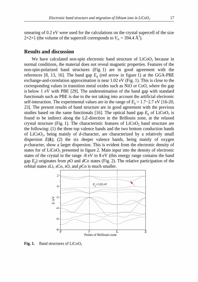
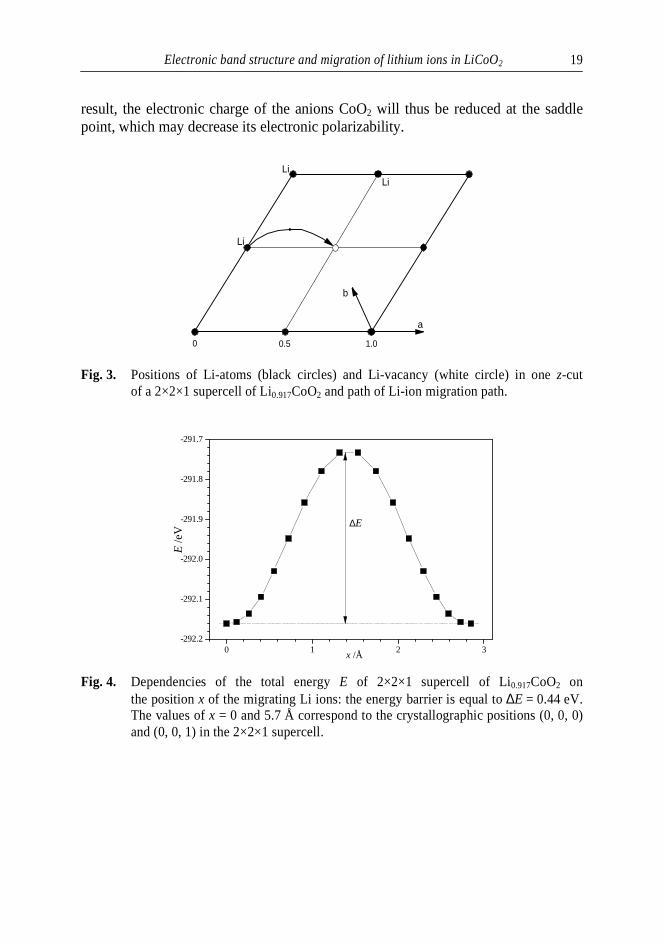
LiCoO2 is a material widely used in solid state batteries, and therefore a study of Li-ions transport properties is important. One of the approaches used by us to study the energy changes of the material at migration of Li ions is NEB method in non-spin polarized calculations, employing the VASP code [28]. A supercell containing 2×2×1 units of the crystallographic unit cell of LiCoO2 (a = b = 5.698 Å, c = 14.023 Å) was generated. The supercell contains 47 atoms and one lithium vacancy (Li0.917CoO2). The NEB images were obtained by moving a Li-ion along the a-axis in the xy-plane towards the vacancy (Fig. 3). The unit cell dimensions were kept fixed during the NEB calculations. The Li-ion migration path from the initial site to the closest vacancy obtained has been found slightly deviated from the straight line. The path and the computed energy barrier obtained ∆E = 0.44 eV (Fig. 4) are in good agreement with the reference results [6, 31].
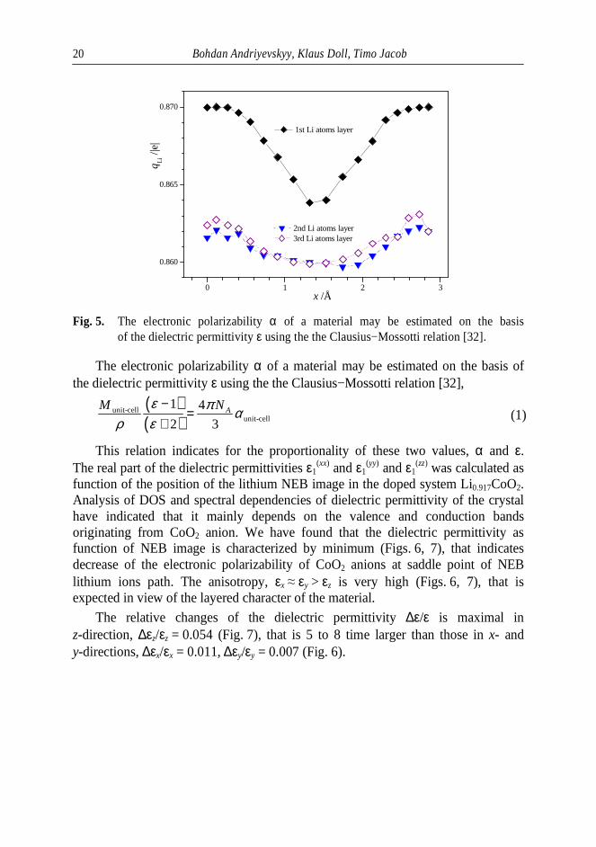
The Bader electronic charges of the Li ions in the three lithium layers of the supercell calculated along the path as a function of the distance between the same NEB images are also characterized by the extremum-like character (Fig. 5). It was found that at the saddle point, where the total energy is at its maximum, the Bader electronic charge for lithium is about −2.136 |e| (the total charge is 0.864 |e|) (Fig. 5). Thus, the total charge of lithium ion is here of the smallest absolute magnitude in relation to charges at other NEB images along the migration path. This means that LiCoO2 here is least ionic. Here, the lithium – oxygen distances become the smallest, that probably influences this reduced iconicity of the material. As a
-5 0 50
1
2
3
dCo pO
PD
OS
/ele
ctro
ns/e
V
E /eV
Eg
Electronic band structure and migration of lithium ions in LiCoO2 19
result, the electronic charge of the anions CoO2 will thus be reduced at the saddle point, which may decrease its electronic polarizability.
Fig. 3. Positions of Li-atoms (black circles) and Li-vacancy (white circle) in one z-cut of a 2×2×1 supercell of Li0.917CoO2 and path of Li-ion migration path.
Fig. 4. Dependencies of the total energy E of 2×2×1 supercell of Li0.917CoO2 on the position x of the migrating Li ions: the energy barrier is equal to ∆E = 0.44 eV. The values of x = 0 and 5.7 Å correspond to the crystallographic positions (0, 0, 0) and (0, 0, 1) in the 2×2×1 supercell.
a
b
0 0.5 1.0
Li
Li
Li
0 1 2 3-292.2
-292.1
-292.0
-291.9
-291.8
-291.7
E /e
V
x /Å
∆E
Bohdan Andriyevskyy, Klaus Doll, Timo Jacob 20
Fig. 5. The electronic polarizability α of a material may be estimated on the basis of the dielectric permittivity ε using the the Clausius−Mossotti relation [32].
The electronic polarizability α of a material may be estimated on the basis of the dielectric permittivity ε using the the Clausius−Mossotti relation [32],
( )( )
unit-cellunit-cell
1 4
2 3AM Nε π α
ρ ε−
=+
(1)
This relation indicates for the proportionality of these two values, α and ε. The real part of the dielectric permittivities ε1
(xx) and ε1(yy) and ε1
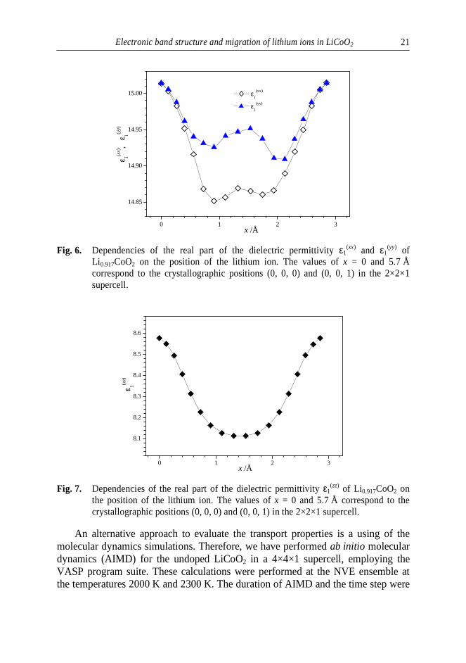
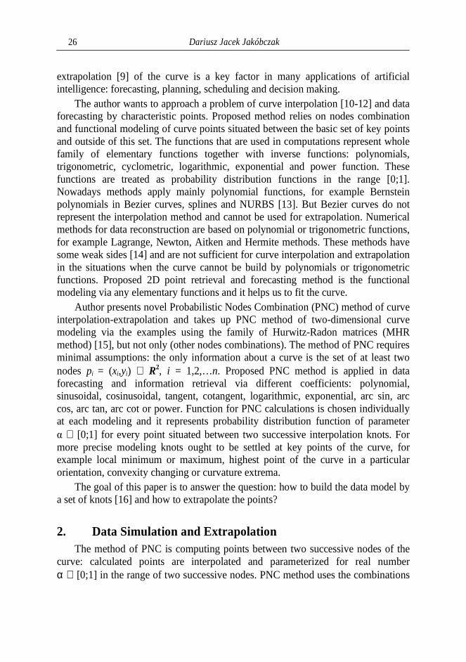
(zz) was calculated as function of the position of the lithium NEB image in the doped system Li0.917CoO2. Analysis of DOS and spectral dependencies of dielectric permittivity of the crystal have indicated that it mainly depends on the valence and conduction bands originating from CoO2 anion. We have found that the dielectric permittivity as function of NEB image is characterized by minimum (Figs. 6, 7), that indicates decrease of the electronic polarizability of CoO2 anions at saddle point of NEB lithium ions path. The anisotropy, εx ≈ εy > εz is very high (Figs. 6, 7), that is expected in view of the layered character of the material.
The relative changes of the dielectric permittivity ∆ε/ε is maximal in z-direction, ∆εz/εz = 0.054 (Fig. 7), that is 5 to 8 time larger than those in x- and y-directions, ∆εx/εx = 0.011, ∆εy/εy = 0.007 (Fig. 6).
0 1 2 3
0.860
0.865
0.870
1st Li atoms layer
2nd Li atoms layer 3rd Li atoms layer
q Li /|
e|
x /Å
Electronic band structure and migration of lithium ions in LiCoO2 21
Fig. 6. Dependencies of the real part of the dielectric permittivity ε1(xx) and ε1
(yy) of Li 0.917CoO2 on the position of the lithium ion. The values of x = 0 and 5.7 Å correspond to the crystallographic positions (0, 0, 0) and (0, 0, 1) in the 2×2×1 supercell.
Fig. 7. Dependencies of the real part of the dielectric permittivity ε1(zz) of Li0.917CoO2 on
the position of the lithium ion. The values of x = 0 and 5.7 Å correspond to the crystallographic positions (0, 0, 0) and (0, 0, 1) in the 2×2×1 supercell.
An alternative approach to evaluate the transport properties is a using of the molecular dynamics simulations. Therefore, we have performed ab initio molecular dynamics (AIMD) for the undoped LiCoO2 in a 4×4×1 supercell, employing the VASP program suite. These calculations were performed at the NVE ensemble at the temperatures 2000 K and 2300 K. The duration of AIMD and the time step were
0 1 2 3
14.85
14.90
14.95
15.00 ε1
(xx)
ε1
(yy)
ε 1(xx),
ε 1(yy)
x /Å
0 1 2 3
8.1
8.2
8.3
8.4
8.5
8.6
ε 1(zz)
x /Å

Bohdan Andriyevskyy, Klaus Doll, Timo Jacob 22
5 ps and 1 fs, correspondingly. Slope of the linear dependency between the mean square displacement (MSD) of lithium ions and the simulation time is the diffusion coefficient D. The activation energy Ea and the value D0 were calculated on the basis of AIMD results at two temperatures mentioned above using the relation of the Arrhenius law type
D = a2ω⋅exp(−Ea/kBT), (2)
where a is the hopping distance (a ≈ 3 Å for LiCoO2), ω is the hopping frequency (ω ≈ 1⋅1013 s-1), and kB is Boltzmann’s constant [33]. Activation energy Ea is one of the main characteristics presenting suitability of a material to the lithium ions batteries. The activation energy obtained in such a way was found to be Ea = 0.5 eV. This value is close to the similar one obtained using the NEB method (Fig. 4).
Conclusions Main parameters of the electronic band structure of LiCoO2 have been
calculated using ab initio calculations within the density functional theory. The computed band gap is found to be Eg = 1.02 eV using the GGA-PBE exchange-and-correlation functional.
Using the nudged elastic band method, the minimal energy barrier of 0.44 eV for lithium ions migration in LiCoO2 has been obtained, that is in agreement with reference data. The electronic polarizability of LiCoO2, which is proportional to the corresponding dielectric permittivity, was found to have a minimum at the trajectory point corresponding to the maximum of total crystal energy. The reduced polarizability of CoO2 observed here takes place due to the reduced ionicity of LiCoO2 found from the Mulliken charges of the material.
The activation energy for lithium ion displacement was also calculated using the molecular dynamics method. Assuming an Arrhenius law, the activation energy of Ea
(Li) = 0.5 eV was deduced, being close to the value obtained with the nudged elastic band method (0.44 eV).
Acknowledgements The CASTEP calculations were performed in the computer center of Wrocław
University of Technology (WCSS) within Accelrys Materials Studio 6.1 package. The VASP calculations were done in the computer center of Warsaw University (ICM) in the framework of the project G26-3.

Electronic band structure and migration of lithium ions in LiCoO2 23
References 1. J.R. Owen, Chem. Soc. Rev. 26, 259 (1997). 2. M. Wakihara, O. Yamamoto (Eds.), Lithium Ion Batteries: Fundamentals and
Performance (WileyVCH, Weinheim, Germany, 1998). 3. A. Van der Ven, M. K. Aydinol, G. Ceder, G. Kresse, J. Hafner, Phys. Rev. B 58,
2975 (1998). 4. M. Landstorfer, T. Jacob, Phys. Chem. Chem. Phys. 13, 12817 (2011). 5. M. Landstorfer, T. Jacob, Chem. Soc. Rev. 42, 3234 (2013). 6. X. Zhu, C. Shen Ong, X. Xu, B. Hu, J. Shang, H. Yang, S. Katlakunta, Y. Liu,
X. Chen, L. Pan, J. Ding, R.-W. Li, Sci. Rep. 3, 1084 (2013). 7. M.T. Czyzyk, R. Potze, G.A. Sawatzky, Phys. Rev. B 46, 3729 (1992). 8. M.K. Aydinol, A.F. Kohan, G. Ceder, Phys. Rev. B 56, 1354 (1997). 9. M. Catti, Phys. Rev. B 61, 1795 (2000). 10. V.R. Galakhov, V.V. Karelina, D.G. Kellerman, V.S. Gorshkov,
N.A. Ovechkina, M. Neumann, Phys. Solid State 44, 266 (2002). 11. D. Carlier, A. Van der Ven, C. Delmas, G. Ceder, Chem. Mater. 15, 2651
(2003). 12. L.Y. Hu, Z.H. Xiong, C.Y. Ouyang, S. Shi, Y. Ji, M. Lei, Z. Wang, H. Li,
X. Huang, L. Chen, Phys. Rev. B 71, 125433 (2005). 13. S. Laubach, S. Laubach, P.C. Schmidt, D. Ensling, S. Schmid, W. Jaegermann,
A. Thißen, K. Nikolowski, H. Ehrenberg, Phys. Chem. Chem. Phys. 11, 3278 (2009).
14. G. Mattioli, M. Risch, A.A. Bonapasta, H. Dau, L. Guidoni, Phys. Chem. Chem. Phys. 13, 15437 (2011).
15. D. Carlier, J.-H. Cheng, C.-J. Pan, M. Ménétrier, C. Delmas, B.-J. Hwang, J. Phys. Chem. C 117, 26493 (2013).
16. D. Ensling, A. Thissen, S. Laubach, P.C. Schmidt, W. Jaegermann, Phys. Rev. B 82, 195431 (2010).
17. P. Ghosh, S. Mahanty, M.W. Raja, R.N. Basu, H.S. Maiti, J. Mater. Res. 22, 1162 (2007).
18. K. Kushida, K. Kuriyama, Solid State Commun. 118, 615 (2001). 19. J.M. Rosolen, F. Decker, J. Electroanalyt. Chem. 501, 253 (2001). 20. M.C. Rao, O.M. Hussain, Eur. Phys. J. Appl. Phys. 48, 20503 (2009). 21. T.A. Hewston, B. Chamberland, J. Phys. Chem. Solids 48, 97 (1987) (and
references cited therein). 22. I. Tomeno, M. Oguchi, J. Phys. Soc. Japan 67, 318 (1998).

Bohdan Andriyevskyy, Klaus Doll, Timo Jacob 24
23. J. van Elp, J.L. Wieland, H. Eskes, P. Kuiper, G.A. Sawatzky, F.M.F. de Groot, T.S. Turner, Phys. Rev. B 44, 6090 (1991).
24. M.P. O’Callaghan, E.J. Cussen, Solid State Sci. 10, 390 (2008). 25. S.J. Clark, M.D. Segall, C.J. Pickard, P.J. Hasnip, M.J. Probert, K. Refson, M.C.
Payne, Zeitschrift für Kristallographie 220, 567 (2005). 26. J.P. Perdew, K. Burke, M. Ernzerhof, Phys. Rev. Lett. 77, 3865 (1996). 27. D. Vanderbilt, Phys. Rev. B 41, 7892 (1990). 28. G. Kresse, D. Joubert, Phys. Rev. 59, 1758 (1999); The guide of VASP
https://cms.mpi.univie.ac.at/marsweb/index.php. 29. T. Bredow, A.R. Gerson, Phys. Rev. B 61, 5194 (2000). 30. http://theory.cm.utexas.edu/vtsttools/neb.html 31. A. Van der Ven, C. Ceder, Phys. Rev. B 64, 184307 (2001). 32. P. Van Rysselberghe, J. Phys. Chem. 36, 1152 (1932). 33. H. Moriwake, A. Kuwabara, C.A.J. Fisher, R. Huang, T. Hitosugi, Y.H. Ikuhara,
H. Oki, Y. Ikuhara, Adv. Mater. 25 618 (2013).
Abstract In view of search the effective materials for the electrochemical sources of
energy, the density functional theory (DFT) based approach has been applied to the computational study of lithium ion migration in LiCoO2. Apart the standard first principles study of band structure and density of electronic states of the crystal, the material was studied using the nudget elastic band (NEB) and the ab initio molecular dynamics (AIMD) methods. The activation energy Ea of the lithium ions self-diffusion in LiCoO2, as one of the main characteristic of the material for the electrochemical sources of energy, has been obtained using NEB (0.44 eV) and AIMD (0.5 eV).
Streszczenie Ze względu na poszukiwanie efektywnych materiałów do baterii
elektrochemicznych, zostały wykonane obliczenia komputerowe z pierwszych zasad na bazie teorii funkcjonału gęstości (density functional theory) struktury elektronowej oraz migracji jonów litu w krysztale LiCoO2. Oprócz standardowych obliczeń struktury pasmowej i gęstości stanów elektronowych, przeprowadzono także badania materiału metodami NEB (Nudget Elastic Bands) i AIMD (Ab Initio Molecular Dynamics). Otrzymano jeden z głównych parametrów migracji litu w krysztale LiCoO2, stosowanym w bateriach elektrochemicznych - energię aktywacji samodyfuzji Ea. Ta wielkość okazała się być w granicach od 0.44 eV (NEB) do 0.5 eV (AIMD).

Dariusz Jacek Jakóbczak Katedra Podstaw Informatyki i Zarządzania Wydział Elektroniki i Informatyki Politechnika Koszalińska
Data Forecasting and Extrapolation via Probability Distribution and Nodes Combination
Keywords: information retrieval, data extrapolation, curve interpolation, PNC method, probabilistic modeling, forecasting
1. Introduction Information retrieval and data forecasting are still the opened questions not only
in mathematics and computer science. For example the process of planning can meet such a problem: what is the next value that is out of our knowledge, for example any wanted value by tomorrow. This planning may deal with buying or selling, with anticipating costs, expenses or with foreseeing any important value. The key questions in planning and scheduling, also in decision making and knowledge representation [1] are dealing with appropriate information modeling and forecasting. Two-dimensional data can be regarded as points on the curve. Classical polynomial interpolations and extrapolations (Lagrange, Newton, Hermite) are useless for data forecasting, because values that are extrapolated (for example the stock quotations or the market prices) represent continuous or discrete data and they do not preserve a shape of the polynomial. This paper is dealing with data forecasting by using the method of Probabilistic Nodes Combination (PNC) and extrapolation as the extension of interpolation. The values which are retrieved, represented by curve points, consist of information which allows us to extrapolate and to forecast some data for example before making a decision [2].
If the probabilities of possible actions are known, then some criteria are to be applied: Laplace, Bayes, Wald, Hurwicz, Savage, Hodge-Lehmann [3] and others [4]. But this paper considers information retrieval and data forecasting based only on 2D nodes. Proposed method of Probabilistic Nodes Combination (PNC) is used in data reconstruction and forecasting. PNC method uses two-dimensional data for knowledge representation [5] and computational foundations [6]. Also medicine [7], industry and manufacturing are looking for the methods connected with geometry of the curves [8]. So suitable data representation and precise reconstruction or
Dariusz Jacek Jakóbczak 26
extrapolation [9] of the curve is a key factor in many applications of artificial intelligence: forecasting, planning, scheduling and decision making.
The author wants to approach a problem of curve interpolation [10-12] and data forecasting by characteristic points. Proposed method relies on nodes combination and functional modeling of curve points situated between the basic set of key points and outside of this set. The functions that are used in computations represent whole family of elementary functions together with inverse functions: polynomials, trigonometric, cyclometric, logarithmic, exponential and power function. These functions are treated as probability distribution functions in the range [0;1]. Nowadays methods apply mainly polynomial functions, for example Bernstein polynomials in Bezier curves, splines and NURBS [13]. But Bezier curves do not represent the interpolation method and cannot be used for extrapolation. Numerical methods for data reconstruction are based on polynomial or trigonometric functions, for example Lagrange, Newton, Aitken and Hermite methods. These methods have some weak sides [14] and are not sufficient for curve interpolation and extrapolation in the situations when the curve cannot be build by polynomials or trigonometric functions. Proposed 2D point retrieval and forecasting method is the functional modeling via any elementary functions and it helps us to fit the curve.
Author presents novel Probabilistic Nodes Combination (PNC) method of curve interpolation-extrapolation and takes up PNC method of two-dimensional curve modeling via the examples using the family of Hurwitz-Radon matrices (MHR method) [15], but not only (other nodes combinations). The method of PNC requires minimal assumptions: the only information about a curve is the set of at least two nodes pi = (xi,yi) ∈ R2, i = 1,2,…n. Proposed PNC method is applied in data forecasting and information retrieval via different coefficients: polynomial, sinusoidal, cosinusoidal, tangent, cotangent, logarithmic, exponential, arc sin, arc cos, arc tan, arc cot or power. Function for PNC calculations is chosen individually at each modeling and it represents probability distribution function of parameter α ∈ [0;1] for every point situated between two successive interpolation knots. For more precise modeling knots ought to be settled at key points of the curve, for example local minimum or maximum, highest point of the curve in a particular orientation, convexity changing or curvature extrema.
The goal of this paper is to answer the question: how to build the data model by a set of knots [16] and how to extrapolate the points?
2. Data Simulation and Extrapolation The method of PNC is computing points between two successive nodes of the
curve: calculated points are interpolated and parameterized for real number α ∈ [0;1] in the range of two successive nodes. PNC method uses the combinations

Data Forecasting and Extrapolation via Probability Distribution … 27
of nodes p1=(x1,y1), p2=(x2,y2),…, pn=(xn,yn) as h(p1,p2,…,pm) and m = 1,2,…n to interpolate second coordinate y as (2) for first coordinate c in (1):
c = α⋅xi + (1-α)⋅xi+1, i = 1,2,…n-1, (1)
),...,,()1()1()( 211 mii ppphyycy ⋅−+−+⋅= + γγγγ , (2)
α ∈ [0;1], γ = F(α) ∈[0;1], F:[0;1]→[0;1], F(0)=0, F(1)=1 and F is strictly monotonic.
PNC extrapolation requires α outside of [0;1]: α < 0 (anticipating points right of last node for c > xn) or α > 1 (extrapolating values left of first node for c < x1), γ=F(α), F:P→R, ]1;0[⊃P , F(0)=0, F(1)=1. Here are the examples of h computed for MHR method [17]:
12
22
1
121 ),( x
x
yx
x
ypph += (3)
or
)(1
)(1
),,,(
43224344122124
22
34114333212123
21
4321
yxxyxxyxxyxxxx
yxxyxxyxxyxxxx
pppph
−+++
+
+−+++
=.
Three other examples of nodes combinations:
12
12
21
2121 ),(
yx
xy
yx
xypph += or 212121 ),( yyxxpph += or the simplest
0),...,,( 21 =mppph .
Nodes combination is chosen individually for each data and it depends on the type of information modeling. Formulas (1)-(2) represent curve parameterization as α ∈ P:
x(α) = α⋅xi + (1-α)⋅xi+1 and
),...,,())(1)(())(1()()( 211 mii ppphFFyFyFy ⋅−+−+⋅= + ααααα ,
1211 )),...,,())(1(()()( ++ +⋅−+−⋅= imii yppphFyyFy ααα .
Proposed parameterization gives us the infinite number of possibilities for calculations (determined by choice of F and h) as there is the infinite number of data for reconstruction and forecasting. Nodes combination is the individual feature of each modeled data. Coefficient γ = F(α) and nodes combination h are key factors in PNC interpolation and forecasting.

Dariusz Jacek Jakóbczak 28
2.1. Extended distribution functions in PNC forecasting Points settled between the nodes are computed using PNC method. Each real
number c ∈ [a;b] is calculated by a convex combination c = α ⋅ a + (1 - α) ⋅ b for
ab
cb
−−=α ∈[0;1]. Key question is dealing with coefficient γ in (2). The simplest
way of PNC calculation means h = 0 and γ = α (basic probability distribution). Then PNC represents a linear interpolation and extrapolation. MHR method [18] is not a linear interpolation. MHR [19] is the example of PNC modeling. Each interpolation requires specific distribution of parameter α and γ (1)-(2) depends on parameter α ∈ [0;1]:
γ = F(α), F:[0;1]→[0;1], F(0) = 0, F(1) = 1 and F is strictly monotonic. Coefficient γ is calculated using different functions (polynomials, power functions, sine, cosine, tangent, cotangent, logarithm, exponent, arc sin, arc cos, arc tan or arc cot, also inverse functions) and choice of function is connected with initial requirements and data specifications. Different values of coefficient γ are connected with applied functions F(α). These functions γ = F(α) represent the examples of probability distribution functions for random variable α∈[0;1] and real number s > 0: γ=αs, γ=sin(αs·π/2), γ=sins(α·π/2), γ=1-cos(αs·π/2), γ=1-coss(α·π/2), γ=tan(αs·π/4), γ=tans(α·π/4), γ=log2(α
s+1), γ=log2
s(α+1), γ=(2α–1)s, γ=2/π·arcsin(αs), γ=(2/π·arcsinα)s, γ=1-2/π·arccos(αs), γ=1-(2/π·arccosα)s, γ=4/π·arctan(αs), γ=(4/π·arctanα)s, γ=ctg(π/2–αs·π/4), γ=ctgs(π/2-α·π/4), γ=2-4/π·arcctg(αs), γ=(2-4/π·arcctgα)s, γ=β·α2+(1-β)·α, γ=β·α4+(1-β)·α,…, γ=β·α2k+(1-β)·α for β∈[0;1] and k∈N or
ααγ s⋅−−= )1(1 .
Functions above, used in γ calculations, are strictly monotonic for random variable α∈[0;1] as γ = F(α) is probability distribution function. There is one important probability distribution in mathematics: beta distribution where for example γ=3α2-2α3, γ=4α3-3α4 or γ=2α-α2. Also inverse functions F-1 are appropriate for γ calculations. Choice of function and value s depends on data specifications and individual requirements during data interpolation.
Extrapolation demands that α is out of range [0;1], for example α∈(1;2] or α∈[-1;0), with γ = F(α) as probability distribution function and then F is called extended distribution function in the case of extrapolation. Some of these functions γ are useless for data forecasting because they do not exist (γ=α½, γ=α¼) if α < 0 in (1). Then it is possible to change parameter α < 0 into corresponding α > 1 and formulas (1)-(2) turn to equivalent equations:
c = α⋅xi+1 + (1-α)⋅xi, i = 1,2,…n-1, (4)
),...,,()1()1()( 211 mii ppphyycy ⋅−+−+⋅= + γγγγ . (5)

Data Forecasting and Extrapolation via Probability Distribution
PNC forecasting for α < 0 or α > 1 uses function for the arguments from ]1;0[⊃P , γ = F(α), F
be strictly monotonic only for α∈[0;1]. Data simulation and modeling for α > 1 is done using the same function γ = F(α) that is earlier defined for
3. PNC Extrapolation and Data TrendsUnknown data are modeled (interpolated or extrapolated) by the choice of
nodes, determining specific nodes combination and probabilistic distribution function to show trend of values: increasing, decreasing or stable. Less complicated models take h(p1,p2,…,pm) = 0 and then the formula of interpolation (2) looks as follows:
1)1()( +−+⋅= ii yycy γγ .
It is linear interpolation for basic probability distribution ( Example 1 Nodes are (1;3), (3;1), (5;3) and (7;3), h = 0, extended distribution extrapolation is computed with (4)-(5) for α > 1:
Fig. 1. PNC for 9 interpolated points between nodes and 9 extrapolated points.
Anticipated points (stable trend): (7.2;3), (7.4;3), (7.6;3), (7.8;3), (8;3), (8.2;3), (8.4;3), (8.6;3), (8.8;3) for α = 1.1, 1.2, …, 1.9.
Data Forecasting and Extrapolation via Probability Distribution … 29
> 1 uses function F as extended distribution function F:P→R, F(0)=0, F(1)=1 and F has to
[0;1]. Data simulation and modeling for α < 0 or α) that is earlier defined for α∈[0;1].
PNC Extrapolation and Data Trends Unknown data are modeled (interpolated or extrapolated) by the choice of
nodes, determining specific nodes combination and probabilistic distribution function to show trend of values: increasing, decreasing or stable. Less complicated
) = 0 and then the formula of interpolation (2) looks as
It is linear interpolation for basic probability distribution (γ = α).
= 0, extended distribution γ = α2, α > 1:
PNC for 9 interpolated points between nodes and 9 extrapolated points.
Anticipated points (stable trend): (7.2;3), (7.4;3), (7.6;3), (7.8;3), (8;3), (8.2;3),

Dariusz Jacek Jakóbczak30
Example 2 Nodes (1;3), (3;1), (5;3) and (7;2), h = 0, extended distribution Forecasting is computed as (4)-(5) with α > 1:
Fig. 2. PNC with 9 interpolated points between nodes and 9 extrapolated points.
Extrapolated points (decreasing trend): (7.2;1.79), (7.4;1.56), (7.6;1.31), (7.8;1.04), (8;0.75), (8.2;0.44), (8.4;0.11), (8.6;-0.24), (8.8; Example 3 Nodes (1;3), (3;1), (5;3) and (7;4), h = 0, extended distribution
Fig. 3. PNC for 9 interpolated points between nodes and 9 extrapolated points.
Forecast (increasing trend): (7.2;4.331), (7.4;4.728), (7.6;5.197), (7.8;5.744), (8;6.375), (8.2;7.096), (8.4;7.913), (8.6;8.832), (8.8;9.859) for
These three examples 1-3 (Fig.1-3) with nodes combination fourth node and extended probability distribution functions possibilities of modeling are connected with a choice of nodes combination
Dariusz Jacek Jakóbczak
= 0, extended distribution γ=F(α)=α2.
PNC with 9 interpolated points between nodes and 9 extrapolated points.
decreasing trend): (7.2;1.79), (7.4;1.56), (7.6;1.31), (7.8;1.04), 0.24), (8.8;-0.61) for α = 1.1, 1.2, …, 1.9.
= 0, extended distribution γ=F(α)=α3:
r 9 interpolated points between nodes and 9 extrapolated points.
Forecast (increasing trend): (7.2;4.331), (7.4;4.728), (7.6;5.197), (7.8;5.744), (8;6.375), (8.2;7.096), (8.4;7.913), (8.6;8.832), (8.8;9.859) for α = 1.1, 1.2, …, 1.9.
3) with nodes combination h = 0 differ at fourth node and extended probability distribution functions γ=F(α). Much more possibilities of modeling are connected with a choice of nodes combination

Data Forecasting and Extrapolation via Probability Distribution
h(p1,p2,…,pm). MHR method [20] uses the combination (3) with good features connected with orthogonal rows and columns at Hurwitz[21-22]:
ii
ii
i
iii x
x
yx
x
ypph
1
111),(
+
+++ +=
and then (2): )1()1()( 1+ ⋅−+−+⋅= ii yycy γγγγHere are two examples 4 and 5 of PNC method with MHR combination (3). Example 4 Nodes are (1;3), (3;1) and (5;3), extended distribution computed with (4)-(5) for α > 1:
Fig. 4. PNC modeling with 9 interpolated points between nodes and 9 extrapolated points.
Extrapolation (decreasing trend): (5.2;2.539), (5.4;1.684), (5.6;0.338), (5.8;(6;-4.25), (6.2;-7.724), (6.4;-12.155), (6.6;for α = 1.1, 1.2, …, 1.9.
Data Forecasting and Extrapolation via Probability Distribution … 31
combination (3) with good features connected with orthogonal rows and columns at Hurwitz-Radon family of matrices
),( 1+ii pph .
Here are two examples 4 and 5 of PNC method with MHR combination (3).
Nodes are (1;3), (3;1) and (5;3), extended distribution γ = F(α) = α2. Forecasting is
PNC modeling with 9 interpolated points between nodes and 9 extrapolated points.
Extrapolation (decreasing trend): (5.2;2.539), (5.4;1.684), (5.6;0.338), (5.8;-1.603), 12.155), (6.6;-17.68), (6.8;-24.443)

Dariusz Jacek Jakóbczak32
Example 5 Nodes (1;3), (3;1) and (5;3), extended distribution computed with (4)-(5) for α > 1:
Fig. 5. PNC modeling with 9 interpolated points between nodes and 9 extrapolated points.
Value forecasting (decreasing trend): (5.2;2.693), (5.4;2.196), (5.6;1.487), (5.8;0.543), (6;-0.657), (6.2;-2.136), (6.4;-for α =1.1, 1.2, …, 1.9.
Now let us consider PNC method with other functions α < 0 for extrapolation (1)-(2) and nodes combination
Example 6 Nodes (2;2), (3;1), (4;2), (5;1), (6;2) and extended distribution
Fig. 6. PNC modeling with 9 interpolated points between nodes and 9 extrapolated points.
Dariusz Jacek Jakóbczak
Nodes (1;3), (3;1) and (5;3), extended distribution γ = F(α) = α1.5. This forecasting is
PNC modeling with 9 interpolated points between nodes and 9 extrapolated points.
Value forecasting (decreasing trend): (5.2;2.693), (5.4;2.196), (5.6;1.487), -3.915), (6.6;-6.016), (6.8;-8.461)
Now let us consider PNC method with other functions F than power functions, (2) and nodes combination h=0.
Nodes (2;2), (3;1), (4;2), (5;1), (6;2) and extended distribution F(α)=sin(α·π/2), h=0:
points between nodes and 9 extrapolated points.

Data Forecasting and Extrapolation via Probability Distribution
Extrapolation points (increasing trend): (6.1;2.156), (6.2;2.309), (6.3;2.454), (6.4;2.588), (6.5;2.707), (6.6;2.809), (6.7;2.891), (6.8;2.951), (6.9;2.988) for α = -0.1, -0.2, …, -0.9. Example 7 Nodes (2;2), (3;1), (4;2), (5;1), (6;2) and extended distrh = 0:
Fig. 7. PNC modeling with nine interpolated points between successive nodes and nine extrapolated points right of the last node.
Forecast points (increasing trend): (6.1;2.004), (6.2;2.03), (6.3;2.094), (6.4;2.203), (6.5;2.354), (6.6;2.53), (6.7;2.707), (6.8;2.86), (6.9;2.964) for 0.9.
These two examples 6 and 7 (Fig.6-7) with nodes combination same set of nodes differ only at extended probability distribution functions Fig.8 is the example of nodes combination h as (3) in MHR method. Example 8 Nodes (2;2), (3;1), (4;1), (5;1), (6;2) and extended distribution function γ=F(α)=2α -1:
Data Forecasting and Extrapolation via Probability Distribution … 33
Extrapolation points (increasing trend): (6.1;2.156), (6.2;2.309), (6.3;2.454), (6.4;2.588), (6.5;2.707), (6.6;2.809), (6.7;2.891), (6.8;2.951), (6.9;2.988)
Nodes (2;2), (3;1), (4;2), (5;1), (6;2) and extended distribution γ=F(α)=sin3(α·π/2),
PNC modeling with nine interpolated points between successive nodes and nine
Forecast points (increasing trend): (6.1;2.004), (6.2;2.03), (6.3;2.094), (6.4;2.203), .5;2.354), (6.6;2.53), (6.7;2.707), (6.8;2.86), (6.9;2.964) for α = -0.1, -0.2, …, -
7) with nodes combination h=0 and the same set of nodes differ only at extended probability distribution functions γ = F(α).
as (3) in MHR method.
Nodes (2;2), (3;1), (4;1), (5;1), (6;2) and extended distribution function
Dariusz Jacek Jakóbczak34
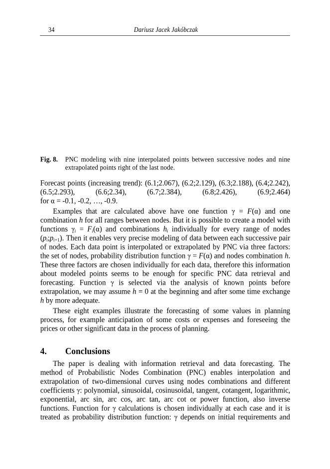
Fig. 8. PNC modeling with nine interpolated points between successive nodes and nine extrapolated points right of the last node.
Forecast points (increasing trend): (6.1;2.067), (6.2;2.129), (6.3;2.188), (6.4;2.242), (6.5;2.293), (6.6;2.34), (6.7;2.384), (6.8;2.426), (6.9;2.464) for α = -0.1, -0.2, …, -0.9.
Examples that are calculated above have one function combination h for all ranges between nodes. But it is possible to create a model with functions γi = Fi(α) and combinations hi individually for every range of nodes (pi;pi+1). Then it enables very precise modeling of data between each successive pair of nodes. Each data point is interpolated or extrapolated by PNC via three factors: the set of nodes, probability distribution function These three factors are chosen individually for each data, therefore this information about modeled points seems to be enough for specific PNC data retrieval and forecasting. Function γ is selected via the analysis of known points before extrapolation, we may assume h = 0 at the beginning and after some time exchange h by more adequate.
These eight examples illustrate the forecasting of some values in planning process, for example anticipation of some costs or expenses and foreseeing the prices or other significant data in the process of planning.
4. Conclusions The paper is dealing with information retrieval and data forecasting. The
method of Probabilistic Nodes Combination (PNC) enables interpolation and extrapolation of two-dimensional curves using nodes combinacoefficients γ: polynomial, sinusoidal, cosinusoidal, tangent, cotangent, logarithmic, exponential, arc sin, arc cos, arc tan, arc cot or power function, also inverse functions. Function for γ calculations is chosen individually at eachtreated as probability distribution function: γ depends on initial requirements and
Dariusz Jacek Jakóbczak
PNC modeling with nine interpolated points between successive nodes and nine
Forecast points (increasing trend): (6.1;2.067), (6.2;2.129), (6.3;2.188), (6.4;2.242), (6.5;2.293), (6.6;2.34), (6.7;2.384), (6.8;2.426), (6.9;2.464)
Examples that are calculated above have one function γ = F(α) and one for all ranges between nodes. But it is possible to create a model with
individually for every range of nodes ). Then it enables very precise modeling of data between each successive pair
of nodes. Each data point is interpolated or extrapolated by PNC via three factors: the set of nodes, probability distribution function γ = F(α) and nodes combination h.
ree factors are chosen individually for each data, therefore this information about modeled points seems to be enough for specific PNC data retrieval and
is selected via the analysis of known points before = 0 at the beginning and after some time exchange
These eight examples illustrate the forecasting of some values in planning process, for example anticipation of some costs or expenses and foreseeing the
data in the process of planning.
The paper is dealing with information retrieval and data forecasting. The method of Probabilistic Nodes Combination (PNC) enables interpolation and
dimensional curves using nodes combinations and different : polynomial, sinusoidal, cosinusoidal, tangent, cotangent, logarithmic,
exponential, arc sin, arc cos, arc tan, arc cot or power function, also inverse calculations is chosen individually at each case and it is
γ depends on initial requirements and
Data Forecasting and Extrapolation via Probability Distribution … 35
data specifications. PNC method leads to point extrapolation and interpolation via discrete set of fixed knots. Main features of PNC method are: PNC method develops a linear interpolation and extrapolation into other functions as probability distribution functions; PNC is a generalization of MHR method via different nodes combinations; nodes combination and coefficient γ are crucial in the process of data probabilistic retrieval and forecasting. Future works are going to precise the choice and features of nodes combinations and coefficient γ, also to implementation of PNC in handwriting and signature recognition.
References 1. Brachman, R.J., Levesque, H.J.: Knowledge Representation and Reasoning.
Morgan Kaufman, San Francisco (2004) 2. Fagin, R., Halpern, J.Y., Moses, Y., Vardi, M.Y.: Reasoning About Knowledge.
MIT Press (1995) 3. Straffin, P.D.: Game Theory and Strategy. Mathematical Association of
America, Washington, D.C. (1993) 4. Watson, J.: Strategy – An Introduction to Game Theory. University of
California, San Diego (2002) 5. Markman, A.B.: Knowledge Representation. Lawrence Erlbaum Associates
(1998) 6. Sowa, J.F.: Knowledge Representation: Logical, Philosophical and
Computational Foundations. Brooks/Cole, New York (2000) 7. Soussen, C., Mohammad-Djafari, A.: Polygonal and Polyhedral Contour
Reconstruction in Computed Tomography. IEEE Transactions on Image Processing 11(13), 1507-1523 (2004)
8. Tang, K.: Geometric Optimization Algorithms in Manufacturing. Computer – Aided Design & Applications 2(6), 747-757 (2005)
9. Kozera, R.: Curve Modeling via Interpolation Based on Multidimensional Reduced Data. Silesian University of Technology Press, Gliwice (2004)
10. Collins II, G.W.: Fundamental Numerical Methods and Data Analysis. Case Western Reserve University (2003)
11. Chapra, S.C.: Applied Numerical Methods. McGraw-Hill (2012) 12. Ralston, A., Rabinowitz, P.: A First Course in Numerical Analysis – Second
Edition. Dover Publications, New York (2001) 13. Schumaker, L.L.: Spline Functions: Basic Theory. Cambridge
Mathematical Library (2007) 14. Dahlquist, G., Bjoerck, A.: Numerical Methods. Prentice Hall, New York (1974)
Dariusz Jacek Jakóbczak 36
15. Jakóbczak, D.: 2D and 3D Image Modeling Using Hurwitz-Radon Matrices. Polish Journal of Environmental Studies 4A(16), 104-107 (2007)
16. Jakóbczak, D.: Shape Representation and Shape Coefficients via Method of Hurwitz-Radon Matrices. Lecture Notes in Computer Science 6374 (Computer Vision and Graphics: Proc. ICCVG 2010, Part I), Springer-Verlag Berlin Heidelberg, 411-419 (2010)
17. Jakóbczak, D.: Curve Interpolation Using Hurwitz-Radon Matrices. Polish Journal of Environmental Studies 3B(18), 126-130 (2009)
18. Jakóbczak, D.: Application of Hurwitz-Radon Matrices in Shape Representation. In: Banaszak, Z., Świć, A. (eds.) Applied Computer Science: Modelling of Production Processes 1(6), pp. 63-74. Lublin University of Technology Press, Lublin (2010)
19. Jakóbczak, D.: Object Modeling Using Method of Hurwitz-Radon Matrices of Rank k. In: Wolski, W., Borawski, M. (eds.) Computer Graphics: Selected Issues, pp. 79-90. University of Szczecin Press, Szczecin (2010)
20. Jakóbczak, D.: Implementation of Hurwitz-Radon Matrices in Shape Representation. In: Choraś, R.S. (ed.) Advances in Intelligent and Soft Computing 84, Image Processing and Communications: Challenges 2, pp. 39-50. Springer-Verlag, Berlin Heidelberg (2010)
21. Jakóbczak, D.: Object Recognition via Contour Points Reconstruction Using Hurwitz-Radon matrices. IGI Global books „Image Processing: Concepts, Methodologies, Tools, and Applications”, Hershey PA, USA, 998-1018 (2013)
22. Jakóbczak, D.: Curve Parameterization and Curvature via Method of Hurwitz-Radon Matrices. Image Processing & Communications- An International Journal 1-2(16), 49-56 (2011)
Abstract Proposed method, called Probabilistic Nodes Combination (PNC), is the method of 2D data interpolation and extrapolation. Nodes are treated as characteristic points of information retrieval and data forecasting. PNC modeling via nodes combination and parameter γ as probability distribution function enables 2D point extrapolation and interpolation. Two-dimensional information is modeled via nodes combination and some functions as continuous probability distribution functions: polynomial, sine, cosine, tangent, cotangent, logarithm, exponent, arc sin, arc cos, arc tan, arc cot or power function. Extrapolated values are used as the support in data forecasting.

Data Forecasting and Extrapolation via Probability Distribution … 37
Streszczenie Autorska metoda Probabilistycznej Kombinacji Węzłów- Probabilistic Nodes Combination (PNC) jest wykorzystywana do interpolacji i ekstrapolacji dwuwymiarowych danych. Węzły traktowane są jako punkty charakterystyczne informacji, która ma być odtwarzana lub przewidywana. Dwuwymiarowe dane są interpolowane lub ekstrapolowane z wykorzystaniem różnych funkcji rozkładu prawdopodobieństwa: potęgowych, wielomianowych, wykładniczych, logarytmicznych, trygonometrycznych, cyklometrycznych. W pracy pokazano propozycję metody ekstrapolowania danych jako pomoc w przewidywaniu trendu dla nieznanych wartości.


Marcin Walczak Katedra Systemów Elektronicznych Wydział Elektroniki i Informatyki Politechnika Koszalińska
Modified small-signal models of BUCK, BOOST and BUCK-BOOST DC-DC converters
Key words: BUCK, BOOST, BUCK-BOOST, line-to-output, control-to-output, parasitic resistance, PWM converters, small signal model, DC-DC converters
Introduction DC-DC converters are circuits consisting of both linear, and nonlinear elements.
Additionally converters work as a switching circuits, therefore even though they consist of few elements the process of modeling is not as simple as in common circuits.
The first method of modeling the converters was presented in year 1976 and it was based on averaging of state space equations [1]. Since then converters have been described using various techniques e.g. switch averaging [2], [3] and separation of variables [4], [5], which was used to derive models presented in this paper. All of those methods have one in common - they are based on averaging signals over one switching cycle. The most popular models which can be found in the literature describe ideal converters, some of them include few parasitic resistances [2], [3], [6]. One can also find models considering parasitic resistances, which describe most losses in converter circuit [7], [8].
The authors who neglect some of parasitic resistances, probably are assuming that the losses are so small that ignoring them won't make a change in the model. Such assumption is true if parasitic resistances are sufficiently small [9]. However in some cases it is not possible to use the simpler model and thus the full model needs to be used [10].
In order to model the behavior of a converter, besides all other parasitic resistances, one can use static or dynamic model of diode resistance. The model considering dynamic resistance of a diode is more universal because, if needed, it is much easier to switch to the model with static resistance than opposite. Most models that can be found in literature do not include the dynamic resistance and voltage offset of a diode [1], [7], [11]. Therefore those models are limited in use. However

Marcin Walczak 40
there are some papers that include models considering both the diode resistance and voltage offset [8], [12] which allows to analyze an influence of additional parameter.
This paper contains models of converters working in the continuous conduction mode (CCM). The models consider the dynamic value of diode resistance and a voltage offset, created after linearization of diode characteristic. First chapter describes basic terms and nomenclature used in further part of this paper.
From the second to the fourth chapter one can find derived models of BUCK, BOOST and BUCK-BOOST converters, which can be used to simulate work of the converters. The models consider dynamic value of diode resistance and the voltage offset, as it has been mentioned previously.
The fifth chapter is used to present some Scilab simulations of models presented in this paper in comparison to known models [12].
The fifth chapter is followed by conclusion and references.
1. Static and dynamic diode resistance When modeling an ideal DC-DC converter (figure 1) one doesn’t need to
consider parasitic resistances of its electronic components. When considering non ideal power converter one needs to specify values of parasitic resistances, which are a simple representation of power loses.
Fig. 1. An ideal step-down converter (BUCK) consisting of ideal transistor T, diode D, inductor L and capacitor C.
Modified small-signal models of BUCK, BOOST … 41
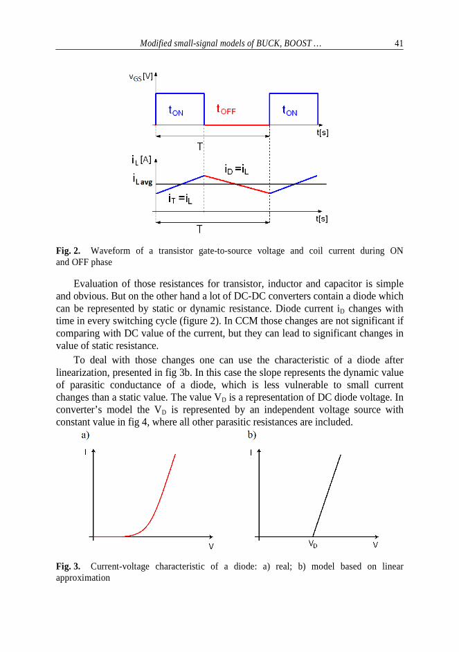
Fig. 2. Waveform of a transistor gate-to-source voltage and coil current during ON and OFF phase
Evaluation of those resistances for transistor, inductor and capacitor is simple and obvious. But on the other hand a lot of DC-DC converters contain a diode which can be represented by static or dynamic resistance. Diode current iD changes with time in every switching cycle (figure 2). In CCM those changes are not significant if comparing with DC value of the current, but they can lead to significant changes in value of static resistance.
To deal with those changes one can use the characteristic of a diode after linearization, presented in fig 3b. In this case the slope represents the dynamic value of parasitic conductance of a diode, which is less vulnerable to small current changes than a static value. The value VD is a representation of DC diode voltage. In converter’s model the VD is represented by an independent voltage source with constant value in fig 4, where all other parasitic resistances are included.
Fig. 3. Current-voltage characteristic of a diode: a) real; b) model based on linear approximation

Marcin Walczak 42
2. Models of BUCK converter with all parasitic resistances To create a mathematical model of a converter means to calculate it’s transfer
function. In this paper two important transfer functions are considered. One of them represent the response of output voltage to input voltage excitation and it is called line-to-output transfer function (1). The second transfer function represent dependency of output voltage on small-signal duty cycle and it is called control-to-output transfer function (2).
0)()(
)()(
=
=sg
og sV
sVsH
θ
(1)
0)()(
)()(
=
=sV
od
gs
sVsH
θ (2)
where: Hg(s) - transfer function line-to-output Hd(s) - transfer function control-to-output Vo(s) - small signal value of output voltage
θ(s) - small signal value of duty ratio DC-DC converters are switching circuits hence when calculating the transfer
function it is necessary to use one of averaging techniques presented in [2] [4] [5] [12]. All those techniques are based on averaging currents and/or voltages over one switching cycle. After averaging a linearization takes place where all signals are treated as a combination of a constant, and a small signal values as presented in (3).
)(txXx += (3)
The linearization is followed by separation of the small signal values from the constant values. The small signal values are used to calculate the transfer functions accordingly to (1), (2).
An implementation of diode model considering the dynamic resistance RD, and voltage offset VD, into a BUCK converter consisting of real elements is presented in figure 4

Modified small-signal models of BUCK, BOOST … 43
Fig. 4. Non ideal BUCK converter consisting of ideal components and their parasitic resistances
Using one of averaging techniques based on separation of variables the BUCK converter transfer functions has been derived:
( , ) 2
(1 )( )
( ) 1A C
g BUCK CCM
Z Z Z C Z
D sCRH s
s C L C R LG CR s GR
+=
+ + + + + (4)
( , ) 2
( ( ) )(1 )( )
( ) 1G L T D D C
d BUCK CCM
Z Z Z C Z
V I R R V sCRH s
s C L C R LG CR s GR
− − − +=
+ + + + + (5)
where: (1 )
1A G D A
OZ
D V V DV
GR
+ −=
+ (6)
(1 )
1A G D A
LZ
D V V DI G
GR
+ −=
+ (7)
(1 )Z CC C GR= + (8)
( )Z A T D L DR D R R R R= − + + (9)
The values VO, VG, VD, IL, and DA are constant values of output voltage, input
voltage, diode offset voltage, coil current and duty ratio respectively. Equations (6) – (7) have been derived after linearization and separation of the small signal values from the constant values.
Accordingly to (4) the value of diode voltage offset VD in BUCK converter doesn't influence the transfer function Hg(s). It means that only change of static to dynamic resistance affects this transfer functions. The equation (4) is not different from the one presented in [5][14] except that here the value of RD refers to the dynamic resistance.

Marcin Walczak 44
3. Models of BOOST converter Circuit of a BOOST converter considering all parasitic resistances and model of
a diode with dynamic resistance and voltage offset is presented in figure 5
Fig. 5. Circuit of a BOOST converter considering all parasitic resistances and model of a diode with dynamic resistance and voltage offset
Transfer functions related to the circuit presented in figure 5 are presented in (10) and (11):
( , ) 2 2 2
(1 )(1 )( )
( (1 ) ) (1 )C A
g BOOST CCMZ Z Z C A Z A
sCR DH s
s LC s C R GL CR D GR D
+ −=
+ + + − + + − (10)
( , ) 2 2 2
( )(1 )(1 )( ( ) )
(1 )( )
( (1 ) ) (1 )
L ZC A L T D D O
Ad BOOST CCM
Z Z Z C A Z A
I sL RsCR D I R R V V
DH s
s LC s C R GL CR D GR D
++ − − − + + −
−=
+ + + − + + − (11)
where for BOOST converter:
2
(1 )(1 )
(1 )G D A
O AZ A
V V DV D
R G D
− −= −
+ − (12)
2
(1 )
(1 )G D A
L
Z A
V V DI G
R G D
− −=
+ − (13)
Formulas related to CZ and RZ have been presented in (8) and (9).
4. Models of BUCK-BOOST converter In figure 6 one can find a circuit of BUCK-BOOST converter which was used
to derive transfer functions (14) and (15). The circuit contains all parasitic resistances and model of a diode considering dynamic resistance and voltage offset.

Modified small-signal models of BUCK, BOOST … 45
Fig. 6. Circuit of a BUCK-BOOST converter, including all parasitic resistances and model of a diode considering dynamic resistance and voltage offset
Small signal models related to the circuit in figure 6 are presented in (14) and (15)
( , ) 2 2 2
(1 )(1 )
( (1 ) ) (1 )C A A
g BUCK BOOST CCM
z z Z C A Z A
sCR D DH
s LC s C R LG CR D GR D−+ −
=+ + + − + + −
(14)
( , ) 2 2 2
( )(1 )(1 ) ( )
(1 )
( (1 ) ) (1 )
L ZC A G L L D O D
Ad BUCK BOOST CCM
z z Z C A Z A
I sL RsCR D V I R R V V
DH
s LC s C R LG CR D GR D−
++ − − + − + + + − =
+ + + − + + − (15)
Constant values of output voltage and coil current can be calculated with (16) and (17):
2
2
(1 ) (1 )
(1 )G A A D A
OZ A
V D D V DV
GR D
− − + −=
− − (16)
2
(1 )
(1 )G A D A
L
Z A
V D V DI G
GR D
− + −=
− − (17)
As it was mentioned before, formulas related to CZ and RZ have been presented in (8) and (9).
5. Simulations of BUCK converter In this chapter one can find simulations of a BUCK converter. Values of the
elements, used in following simulations, have been chosen to be in compliance with values of real, measured elements. All those values have been presented in tab. 1.

Marcin Walczak 46
Table 1
VG=5 V C=44,7 μF DA=0,5 RT=4 mΩ RC=35 mΩ G=0,2 S RD_STAT=364 mΩ L=23,5 μH VD=0,8 V RD_DYN=59 mΩ *RL=62 mΩ * Resistance RL includes the value of a resistor used to measure the coil current
5.1. Comparison with other model A large signal model considering diode voltage offset has already been
presented in [12]. The model is presented in figure 7. The differences in nomenclature are explained in tab. 2.
Fig. 7. Large signal model of a BUCK converter presented in [12]
where:
LFDS rRDDrr +−+= )1( (18)
Table 2
Symbol used in [12]
Description Equivalent
symbol used in this paper
vI Input voltage vG
VF Forward voltage of a diode VD
rL ESR of a inductor RL
rC ESR of a capacitor RC
rDS RDS(ON) resistance of a transistor RT
RF Forward resistance of a diode RD
RL Load resistance RO=1/G
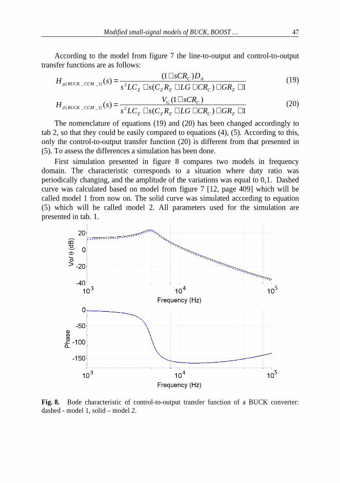
Modified small-signal models of BUCK, BOOST … 47
According to the model from figure 7 the line-to-output and control-to-output transfer functions are as follows:
1)(
)1()(
2)1__( ++++++=
ZCZZZ
ACCCMBUCKg GRCRLGRCsLCs
DsCRsH (19)
1)(
)1()(
2)1__( ++++++=
ZCZZZ
CGCCMBUCKd GRCRLGRCsLCs
sCRVsH (20)
The nomenclature of equations (19) and (20) has been changed accordingly to tab 2, so that they could be easily compared to equations (4), (5). According to this, only the control-to-output transfer function (20) is different from that presented in (5). To assess the differences a simulation has been done.
First simulation presented in figure 8 compares two models in frequency domain. The characteristic corresponds to a situation where duty ratio was periodically changing, and the amplitude of the variations was equal to 0,1. Dashed curve was calculated based on model from figure 7 [12, page 409] which will be called model 1 from now on. The solid curve was simulated according to equation (5) which will be called model 2. All parameters used for the simulation are presented in tab. 1.
Fig. 8. Bode characteristic of control-to-output transfer function of a BUCK converter: dashed - model 1, solid – model 2.
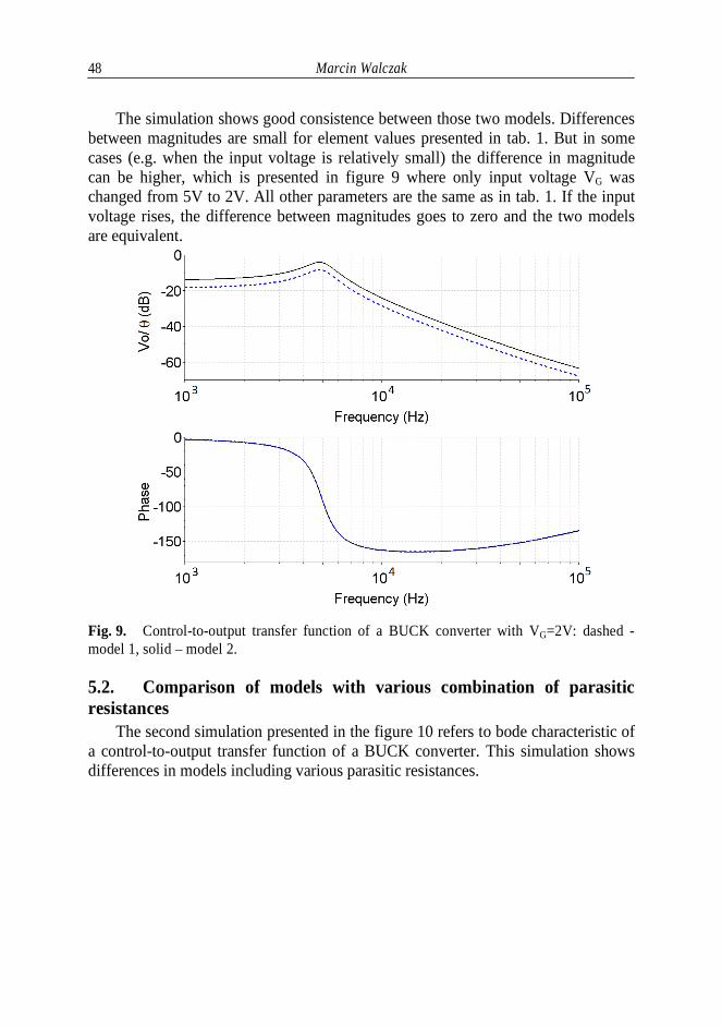
Marcin Walczak 48
The simulation shows good consistence between those two models. Differences between magnitudes are small for element values presented in tab. 1. But in some cases (e.g. when the input voltage is relatively small) the difference in magnitude can be higher, which is presented in figure 9 where only input voltage VG was changed from 5V to 2V. All other parameters are the same as in tab. 1. If the input voltage rises, the difference between magnitudes goes to zero and the two models are equivalent.
Fig. 9. Control-to-output transfer function of a BUCK converter with VG=2V: dashed - model 1, solid – model 2.
5.2. Comparison of models with various combination of parasitic resistances
The second simulation presented in the figure 10 refers to bode characteristic of a control-to-output transfer function of a BUCK converter. This simulation shows differences in models including various parasitic resistances.
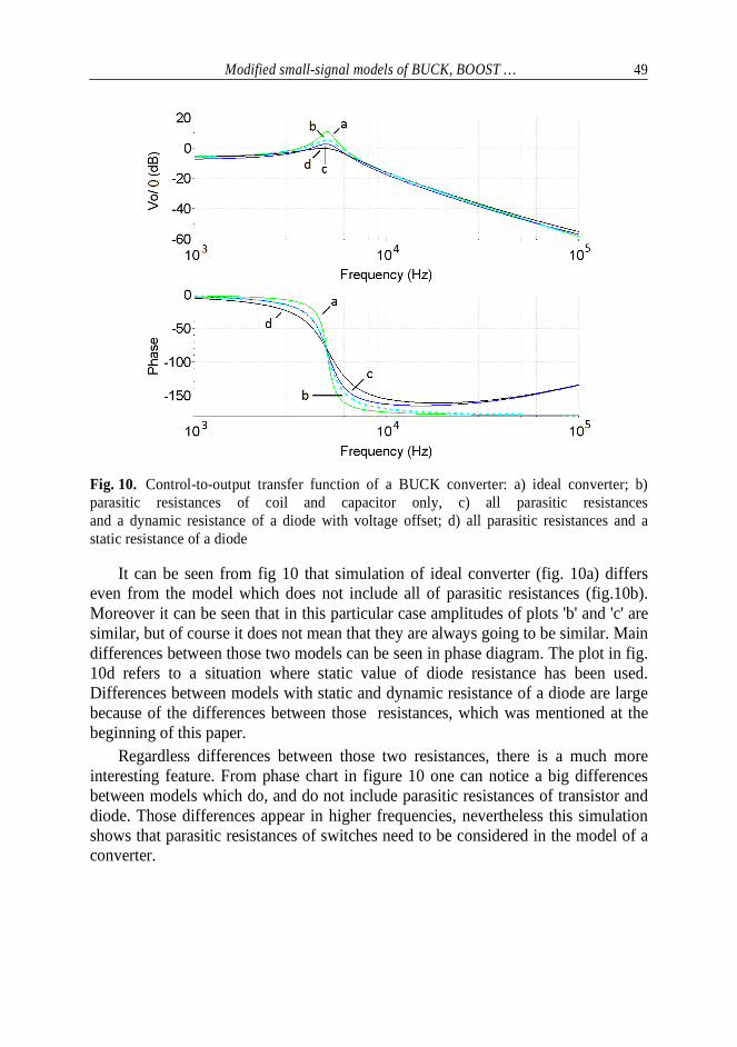
Modified small-signal models of BUCK, BOOST … 49
Fig. 10. Control-to-output transfer function of a BUCK converter: a) ideal converter; b) parasitic resistances of coil and capacitor only, c) all parasitic resistances and a dynamic resistance of a diode with voltage offset; d) all parasitic resistances and a static resistance of a diode
It can be seen from fig 10 that simulation of ideal converter (fig. 10a) differs even from the model which does not include all of parasitic resistances (fig.10b). Moreover it can be seen that in this particular case amplitudes of plots 'b' and 'c' are similar, but of course it does not mean that they are always going to be similar. Main differences between those two models can be seen in phase diagram. The plot in fig. 10d refers to a situation where static value of diode resistance has been used. Differences between models with static and dynamic resistance of a diode are large because of the differences between those resistances, which was mentioned at the beginning of this paper.
Regardless differences between those two resistances, there is a much more interesting feature. From phase chart in figure 10 one can notice a big differences between models which do, and do not include parasitic resistances of transistor and diode. Those differences appear in higher frequencies, nevertheless this simulation shows that parasitic resistances of switches need to be considered in the model of a converter.
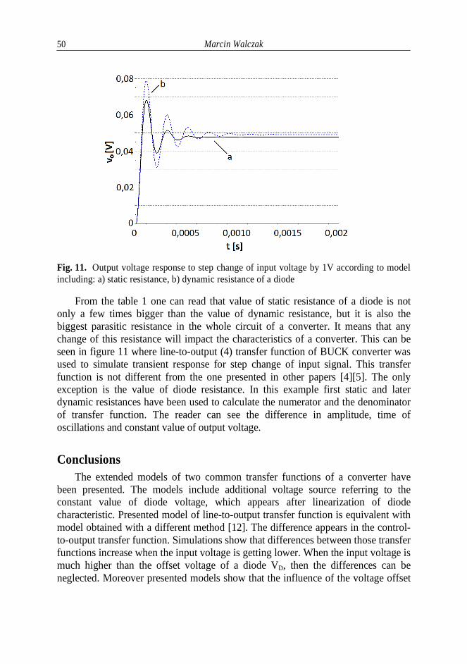
Marcin Walczak 50
Fig. 11. Output voltage response to step change of input voltage by 1V according to model including: a) static resistance, b) dynamic resistance of a diode
From the table 1 one can read that value of static resistance of a diode is not only a few times bigger than the value of dynamic resistance, but it is also the biggest parasitic resistance in the whole circuit of a converter. It means that any change of this resistance will impact the characteristics of a converter. This can be seen in figure 11 where line-to-output (4) transfer function of BUCK converter was used to simulate transient response for step change of input signal. This transfer function is not different from the one presented in other papers [4][5]. The only exception is the value of diode resistance. In this example first static and later dynamic resistances have been used to calculate the numerator and the denominator of transfer function. The reader can see the difference in amplitude, time of oscillations and constant value of output voltage.
Conclusions The extended models of two common transfer functions of a converter have
been presented. The models include additional voltage source referring to the constant value of diode voltage, which appears after linearization of diode characteristic. Presented model of line-to-output transfer function is equivalent with model obtained with a different method [12]. The difference appears in the control-to-output transfer function. Simulations show that differences between those transfer functions increase when the input voltage is getting lower. When the input voltage is much higher than the offset voltage of a diode VD, then the differences can be neglected. Moreover presented models show that the influence of the voltage offset

Modified small-signal models of BUCK, BOOST … 51
is visible only with the control-to-output transfer function. Nevertheless regarding the simulations differences between using static and dynamic resistance of a diode are noticeable in all types of transfer functions.
Presented equations can be easily implemented in a mathematical program such as Scilab or Matlab. To the knowledge of the author all equations of transfer functions presented in this work hadn't been presented before and thus are original extension of models presented in [4][5]. Moreover all models can be very easily modified to use with value of static diode resistance which makes them more practical and universal.
References 1. E.Dijk, H.J.N.Spruijt, D.M. O’Sullivan, J.B. Klaassens, PWM-switch modeling
of DC-DC converters, IEEE Transactions On Power Electronics, Vol. 10, No.6, November (1995)
2. V.Vorperian, Simplified Analysis of PWM converters using model of PWM switch part I: continuous conduction mode, IEEE Transactions On Aerospace And Electronic Systems Vol. 26, No. 3 May (1990)
3. R.D.Middlebrook, S.Cuk, A general unified approach to modeling switching-converter power stages, IEEE Power Electronics Specialists Conference, Cleveland, OH., June 8-10 (1976)
4. W.Janke, Equivalent circuits for averaged description of DC-DC switch-mode power converters based on separation of variables approach, Bulletin Of The Polish Academy Of Sciences Technical Sciences, Vol. 61, No. 3, pp. 711-723 (2013)
5. W.Janke, Averaged models of pulse-modulated DC-DC power converters. Part II: Models based on the separation of variables, Archives Of Electrical Engineering, Vol. 61(4), pp. 633-654 (2012)
6. V.Biolkova, Z.Kolka, D.Biolek, State-space averaging (SSA) revisited: on the accuracy of SSA-based line-to-output frequency responses of switched DC-DC converters, WSEAS Transactions On Circuits And Systems , Issue 2, Vol. 9, February (2010)
7. V.Jha, P.Rai, State space averaged modeling of basic converter topologies, VSRD International Journal of Electrical, Electronics & Communication Engineering, Vol. 2 (6), 566-575 (2012)
8. C.T.Rim, G.B.Joung, G.H.Cho, Practical switch based state-space modeling of DC-DC converters with all parasitics, IEEE Transactions On Power Electronics, Vol. 6, No. 4, October (1991)

Marcin Walczak 52
9. M.Walczak, Symulacje charakterystyk wejściowych i wyjściowych impulsowych przetwornic napięcia stałego w trybie CCM, XIV International Phd Workshop OWD, 20-23 October (2012)
10. M.Jinno, P.Y.Chen, Y.C.Lai, K. Harada, Investigation on the ripple voltage and the stability of SR BUCK converters witch high output current and low output voltage, IEEE Transactions On Industrial Electronics, Vol. 57. No 3. March (2010)
11. R.W.Erickson, D.Maksimovic, Fundamentals of power electronics, second edition, Sixth printing (2004)
12. M.K.Kazimierczuk, Pulse-width modulated DC–DC power converters, J.Wiley (2008)
13. W.Janke, Impulsowe przetwornica napięcia stałego, Wydawnictwo uczelniane Politechniki Koszalińskiej, Monografia nr 269, Koszalin (2014)
Abstract Various models of DC-DC converters have been presented in many references.
This paper provides extended version of a common transfer functions (line-to-output, control-to-output) of three most popular DC-DC converters BUCK, BOOST and BUCK-BOOST. The extension includes all parasitic resistances and additional voltage source created after linearization of diode characteristic.
Streszczenie W dostępnej literaturze istnieje wiele modeli przetwornic napięcia stałego.
Modele te różnią się między innymi rodzajem uwzględnianych rezystancji pasożytniczych. Niniejszy artykuł zawiera modele przetwornic napięcia stałego BUCK, BOOST oraz BUCK-BOOST, wyprowadzone przy pomocy techniki separacji zmiennych. Modele te uwzględniają zarówno rezystancje pasożytnicze wszystkich elementów przetwornicy jak i dodatkowe źródło napięcia powstałe po linearyzacji charakterystyki diody. Słowa kluczowe: BUCK, BOOST, BUCK-BOOST, rezystancje pasożytnicze w przetwornicach napięcia stałego, modele małosygnałowe, przetwornice napięcia stałego
Natalija Maslennikowa Computer Engineering Department, Politechnika Koszalińska E–mail: [email protected] Anatolij Sergiyenko Computer Engineering Department, National Technical University of Ukraine„KPI” E–mail: [email protected]
Scheduling of synchronous dataflow graphs for datapath synthesis
Keywords: data flow graphs (DFG), synchronous dataflow graphs (SDFs), matrix, pipelined datapath design.
Introduction
In personal computers, mobile phones, DSP systems the computational proces-ses are performed, which are repeated with a period coinciding with the input data arrival. These algorithms are represented by the data flow graphs (DFG). DFG is a directed graph, whose nodes represent the operators, and arcs, or dataflows represent the means for the data transmission. Among DFGs the synchronous dataflow graphs (SDFs) are very popular. In SDF each actor generates and consumes a number of variables, which is unchanged from cycle to cycle [1,2].
The homogeneous SDFs, and multirate SDFs are distinguished. In the multirate SDF the number of variables, that are consumed, or generated by a node in a single cycle can be more than one. To simplify the analysis of the multirate SDF it is usually converted into equivalent uniform SDF [2]. The article deals only with homogeneous SDFs. To get the optimal structural solution it is necessary to find the schedule of the algorithm execution in SDF. The article deals with a new scheduling method based on spatial SDF, which provides the fast search for both effective schedule and structure of the datapath.
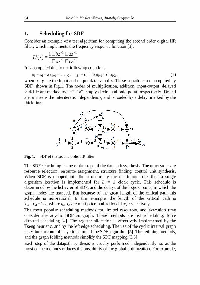
Natalija Maslennikowa, Anatolij Sergiyenko 54
1. Scheduling for SDF Consider an example of a test algorithm for computing the second order digital IIR filter, which implements the frequency response function [3]:
11
11
11
)( −−
−−
++++=
czaz
dzbzzH
It is computed due to the following equations ui = xi − a ui−1 − c ui−2; yi = ui + b ui−1 + d ui−2, (1)
where xi, yi are the input and output data samples. These equations are computed by SDF, shown in Fig.1. The nodes of multiplication, addition, input-output, delayed variable are marked by “+”, “×”, empty circle, and bold point, respectively. Dotted arrow means the interiteration dependency, and is loaded by a delay, marked by the thick line.
Fig. 1. SDF of the second order IIR filter
The SDF scheduling is one of the steps of the datapath synthesis. The other steps are resource selection, resource assignment, structure finding, control unit synthesis. When SDF is mapped into the structure by the one-to-one rule, then a single algorithm iteration is implemented for L = 1 clock cycle. This schedule is determined by the behavior of SDF, and the delays of the logic circuits, in which the graph nodes are mapped. But because of the great length of the critical path this schedule is non-rational. In this example, the length of the critical path is TC = tM + 2tA, where tM, tA are multiplier, and adder delay, respectively. The most popular scheduling methods for limited resources, and execution time consider the acyclic SDF subgraph. These methods are list scheduling, force directed scheduling [4]. The register allocation is effectively implemented by the Tseng heuristic, and by the left edge scheduling. The use of the cyclic interval graph takes into account the cyclic nature of the SDF algorithm [5]. The retiming methods, and the graph folding methods simplify the SDF mapping [3,6]. Each step of the datapath synthesis is usually performed independently, so as the most of the methods reduces the possibility of the global optimization. For example,

Scheduling of synchronous dataflow graphs for datapath synthesis 55
the hardware cost optimization during the resource selection is in contradiction with the cycle time minimizing during the scheduling. Below a method of the datapath synthesis is proposed in which the steps of resource selection, operator scheduling, and resource allocation are implemented in a single step providing the more effective optimization.
2. Spatial SDF and its schedule In [7] the method of the datapath synthesis is described, in which SDF is presented in the three-dimensional space in the form of a triple KG = (K, D, A), where K is the matrix of vectors-nodes Ki, which mean the operators, D is matrix of vectors-edges Dj, performing the links between operators, A is the incidence matrix of SDF. In the vector Ki = (ki, si, ti)
T the coordinates ki, si, ti correspond to the type of operator, the processor unit (PU) number, and the clock cycle. The SDF graph in such a representation is called as spatial SDF. Spatial SDF is splitted into the spatial configuration KGS = (KS, DS, A), and event configuration KGT = (KT, DT, A), which correspond to the datapath structure, and its schedule. By this splitting the vectors Ki = (ki, si, ti)
T are decomposed into vectors KSi = (ki,si)
T, corresponding to the PU coordinates, and vectors KТі = ti, which mean the execution time of the relevant operators in PU KSi. Then the temporal component DТi = ti of the vector Di is equal to the delay of transfer, or processing of the relevant variable. We can assume that the matrix K encodes some acceptable solution, since the matrix D is calculated by the equation
D = KA. (2) The structural optimization consists in finding such a matrix K, which minimizes a given quality criterion. It is possible to specify a matrix DО which provide the minimum value of ТC. Then the vectors Ki are found from a relationship
K = DОAО −1, (3)
where DО is the matrix of vectors-nodes, AО is the incidence matrix of the maximum spanning tree for SDF. When looking for effective structural solution, the following relations have to be considered. Spatial SDF is valid, if the matrix K has no two identical vectors, i.e.
∀ K i,K j (K i ≠ K j, i ≠ j ). (4) The schedule with the period of L clock cycles is correct if the operators, which are mapped into the same PU, are performed in different cycles, i.e.
∀ K i,K j(ki = kj, si = sj ) ⇒ ti ≢ tj mod L . (5) Moreover, the next operator is executed no earlier than the previous one, i.e.
∀Dj ≠DDj (ti ≥ 0). (6)

Natalija Maslennikowa, Anatolij Sergiyenko 56
where DDj is the vector of the interiterational dependence DDj = (kj, sj, –wL)T, which means a delay in w algorithm iterations. The operators of the same type should be mapped into PU of the same type, i.e.
K i,K j∈Kp,q(ki = kj = p, si = sj = q), |Kp,q| ≤ L, (7) where Kp,q is a set of p-type vectors-operators, which are mapped in the q-th PU of p-th type (q = 1,2, ... qp
max). Consider the vectors-edges Dj, including the interiterational dependence vectors DDj, which belong to the i-th graph cycle. Then for it the following equation must be satisfied
∑j
bi,j Dj = (0,0,0)T , (8)
where bi,j is an element of the i-th row of the cyclomatic matrix of SDF. In the simplest case, each operator is executed in a single cycle. This is a natural situation in designing at the RTL level. Complex operators can be calculated for a few cycles. However, when operating in the pipelined mode, the corresponding PU contains stages, each of them has a single cycle delay. Then the search for the schedule consists in the following. The vectors Di ∈ DО are assigned the coordinate ti = 1, i.e. the respective operators have the delays of a single clock cycle. The matrix KT is found from the equation (3). The remaining elements of the matrix DT are found from the equations (2), and (8). If for some of vectors the inequality (6) is not satisfied, then the coordinate ti is increased for certain vectors Di ∈ DО, and the schedule search is repeated. The rest of Ki coordinates are found from the conditions (4) − (8). In such a way the fastest schedule is built, as each statement is executed in a single clock cycle without unnecessary delays. To minimize the searching for coordinates ti in the vectors Di, in [8] the perfect maximum spanning tree of the SDF graph is proposed for the synthesis process. The resulting spatial SDF can be described by the VHDL language, so the pipelined datapath description can be translated into the gate level description by the proper compiler-synthesizer [9].
3. Schedule search example To estimate the method effectiveness consider the schedule searching for SDF in Fig.1. The perfect maximum spanning tree of the SDF is shown in Fig. 2. The additional vector DВ connects the coordinate system origin with an arbitrary node in order to provide the equation (3) consistency.

Scheduling of synchronous dataflow graphs for datapath synthesis 57
Fig. 2. Perfect maximum spanning tree for SDF in Fig. 1
In this example the adder, and pipelined multiplier have one, and two cycle delays, respectively. The following delay matrix is arranged using these delays:
DОТ = ( 1 2 3 4 5 7 8 11 12 13 15 16 B
1 1 1 2 2x1 x2 1 1 1 x3 x4 0 ).
where x1,…,x4 are unknown values, that depend on other vectors in equations (8), whose number is equal to the number of edges minus the number of nodes in SDF. That is, every graph cycle must have at least one edge with the variable delay. So we get a system of four equations (8):
D2 + D4 + D6 + D7 = 0, D3 + D5 + D8 + D14 − D4 − D7 = 0, D2 + D6 + D15 + D9 − D13 = 0, D10 + D14 + D16 − D9 − D11 − D15 = 0.
The solving of this system of equations gives the solution x1 = 1; x2 = 4; x3 = 2; x4 = 7. The algorithm period of L = 4 clock cycles is selected to get a single multiplier unit. Due to (2) the matrix KT is found:
KT = АО ( 1 2 3 4 5 7 8 11 12 13 15 16B
1 1 1 2 2 1 4 1 1 1 2 7 0) = ( 1 2 3 4 5 6 7 8 9 10 11 12 13
5 7 6 5 4 8 4 0 6 7 8 9 10).
The rest of the matrix K elements is obtained according to the equation (4). One should take into account that the number of nodes, standing in one line, which is parallel to the axis ox, approaches to L:
K =
1 2 2 3 3 4 4 4 3 3 2 2 4
0 1 1 2 2 3 3 3 2 2 1 1 4 5 7 6 5 4 8 4 0 6 7 8 9 10
.
A graphic representation of the constructed space SDF is shown in Fig.3. Fig. 4. illustrates the structure of the corresponding digital filter. The small figures in it mark the clock cycles, in which the respective multiplexor inputs, and registers accept the data.
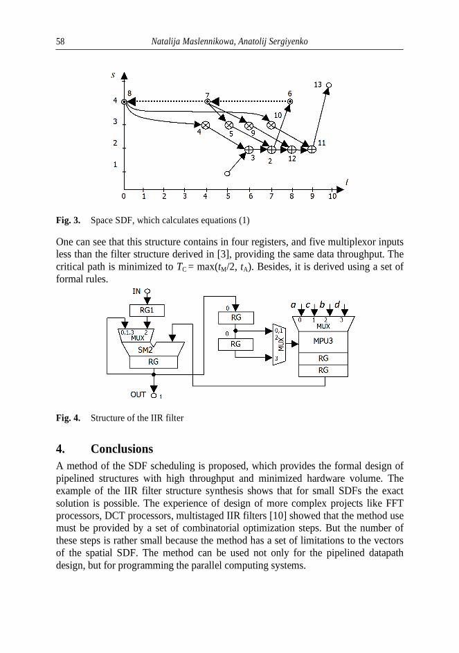
Natalija Maslennikowa, Anatolij Sergiyenko 58
Fig. 3. Space SDF, which calculates equations (1)
One can see that this structure contains in four registers, and five multiplexor inputs less than the filter structure derived in [3], providing the same data throughput. The critical path is minimized to TC = max(tM/2, tA). Besides, it is derived using a set of formal rules.
Fig. 4. Structure of the IIR filter
4. Conclusions A method of the SDF scheduling is proposed, which provides the formal design of pipelined structures with high throughput and minimized hardware volume. The example of the IIR filter structure synthesis shows that for small SDFs the exact solution is possible. The experience of design of more complex projects like FFT processors, DCT processors, multistaged IIR filters [10] showed that the method use must be provided by a set of combinatorial optimization steps. But the number of these steps is rather small because the method has a set of limitations to the vectors of the spatial SDF. The method can be used not only for the pipelined datapath design, but for programming the parallel computing systems.

Scheduling of synchronous dataflow graphs for datapath synthesis 59
References 1. Edwards, S., Lavagno, L., Lee, E.A., Sangiovanny-Vincentelli, A. Design of
Embedded Systems: Formal Models, Validation, and Synthesis, Proc. IEEE, Vol. 85, No. 3, p. 366−390, 1997.
2. Lee, E. A., Messerschmitt D. G. Static scheduling of synchronous data flow programs for digital signal processing. IEEE Trans. on Computers, Vol. 36, No. 1, p. 24−35, 1987.
3. Keshab, K., Parhi, K.K., Chen, Y. Signal Flow Graphs and Data Flow Graphs. In Handbook of Signal Processing Systems, Bhattacharyya, S.S., Deprettere, E.F., Leupers, R. – Ed-s, Springer, p. 791-816, 2010.
4. Paulin, P.G., Knight, J.P. Force – Directed Sheduling for the Behavioral Synthesis of ASICs, IEEE Trans. CAD, −Vol. 7, − No. 3, p. 356−370, 1988.
5. The Systhesis Approach to Digital System Design, Editors P. Micheli, U. Lauther, P. Duzy, Kluwer Academic Pub, 415 p., 1992.
6. Introduction to Scheduling, Y. Robert, and F. Vivien − Ed-s, CRC Press, Taylor and Francis Group, 310 p, 2010.
7. Sergiyenko, A.M., Maslennikow, O., Vinogradow Y. Tensor approach to the application specific processor design, Proc.10th Int. Conf. “The Experience of Designing and Application of CAD Systems in Microelectronics”, CADSM'2009, 24-28 Feb. 2009, IEEE Library, −p. 146−149, 2009.
8. Sergiyenko, A.M. Doskonaly kistyak grafa algorithmu, Vistnyk NTUU−KPI: Informatics, Operation, and Computer Science, No. 46, p. 62−67, 2007. (in Ukrainian)
9. Sergiyenko, A.M. VHDL for Design of Computers, Kiev: DiaSoft, 210 p, 2003. (in Russian)
10. Sergiyenko, A., Uzenkov, O. Low-Pass IIR Filter, 2010. Available at http://opencores.org/project,lp_iir_filter

Natalija Maslennikowa, Anatolij Sergiyenko 60
Summary A method of the schedule searching is proposed, which is based on the properties of the spatial SDF. The method is based on the SDF representation in the multidimensional space. The dimensions of this space are spatial coordinate of the processing unit, time moment of the operator calculation, and operator type. During the synthesis, the nodes are placed in the space according to a set of rules, providing the minimum hardware volume for the given number of clock cycles in the algorithm period. The resulting spatial SDF is described by VHDL language and is modeled and compiled using proper CAD tools. The method is successfully proven by the synthesis of a set of FFT processors, IIR filters, and other pipelined datapaths for FPGA.
Słowa kluczowe: graf zależności informacyjnych (DFG), synchroniczny graf zależności informacyjnych(SDFs), macierz, projektowanie potokowej jednostki przetwarzającej.
Streszczenie Zaproponowany sposób poszukiwania opiera się na właściwościach przestrzennych SDF. Metoda ta bazuje na SDF prezentacji w przestrzeni wielowymiarowej. Wymiarami danej przestrzeni są współrzędne jednostki przetwarzającej, czas momentu obliczeniowego operatora oraz typ operatora. Podczas syntezy, węzły są umieszczone w przestrzeni zgodnie z zestawem reguł, dając minimalną częstotliwość pracy zegara systemowego podczas wykonywania algorytmu. Powstały przestrzenny SDF jest opisany przez język VHDL i jest modelowany i skompilowany przy użyciu odpowiednich narzędzi CAD. Ta metoda jest pomyślnie sprawdzona przez syntezę zestawu procesorów FFT, filtrów IIR, oraz innych potokowych jednostek przetwarzających płytki FPGA.

A.K. Fedotov1, E.A. Streltsov3, I.L. Baranov2, I.A. Svito1, M.V. Malashchonak3, A.V. Mazanik1*
1Physical Faculty, Belarusian State University, Nezalezhnastsi Av. 4, Minsk 220030, Belarus; [email protected];
2Belarusian State University of Informatics and Radioelectronics, P. Brovka 6, Minsk 220013, Belarus; 3Chemical Faculty, Belarusian State University, Nezalezhnastsi Av. 4, Minsk 220030, Belarus;
Magnetoresistive properties of Ni/TiO2/Ti and Ni/SiO2/Si structures: comparative analysis
Keywords: Ni/TiO2/Ti, Ni/SiO2/Si, magnetoresistance
1. Introduction Development of new types of heterostructures based on nanostructured
ferromagnetic metals and semiconductors is of a great fundamental and practical importance because it enables one to hope for the expansion of the operating temperature and frequency ranges of spintronic devices [1]. These structures can be used in 2D matrices for visualization of magnetic field distribution, in information recording and storage devices, highly sensitive magnetic sensors, etc.
For creation of such structures a template-based approach can be used [2]. Porous silicon and aluminum oxides, as well as titanium dioxide nanotubes can be used as templates. Silicon oxide based templates can be produced using different methods

A. Fedotov, I. Baranov, M. Malashchonak, E. Streltsov, I. Svito, A. Mazanik 62
(lithography, ion-track methods, electrochemically, etc.). Templates based on aluminum and titanium oxides with vertical pores are created most often by anodization of corresponding metals.
Titanium dioxide belongs to wide band gap oxide semiconductors (band gap energy Eg=3.1 eV). It is under investigation for more than 40 years as a photocatalyst, sensitive element of gas sensors, photoanode in the dye- and quantum dot sensitized solar cells, material for self-cleaning coatings and biomedical applications [3,4]. At the same time, magnetic and spintronic properties of TiO2 based structures have been studied to a much lesser extent.
Anodic nanotubes of titanium dioxide (TiO2 NTs) are investigated relatively recently (last 15 years, [5,6]). Anodization of metallic titanium in aqueous and non-aqueous solutions containing fluoride ions with concentration 0.05–0.5 М under DC voltage in the range from 1 to 150 V enables one to obtain TiO2 NT arrays with controllable inner and outer diameter, wall thickness, height, density of location on the surface, etc. [7]. For anodic TiO2 NTs the hexagonal ordered structure inherent to the anodic aluminum oxide films is expressed to a much lesser extent. Other distinctions between TiO2 and Al2O3 are related to TiO2 semiconductor properties and pronounced dielectric properties of Al2O3. In particular, this difference manifests itself in possibility of DC cathodic deposition of metals on TiO2 NTs, as well as under UV illumination.
To date, magnetic and magnetotransport properties of the nanoheterostructures obtained by electrochemical deposition of metals on TiO2 NTs have not been studied. Therefore, a comparison of the properties of “ferromagnetic metal/semiconductor” structures obtained using both SiO2/Si and TiO2/Ti templates is of a great scientific interest.
2. Experimental For preparation of Ni/SiO2/Si structures, 1 μm thick SiO2 layer was thermally grown
on the (100) surface of 4.5 Ω∙cm phosphorous doped Cz Si wafer. Using standard photolithography procedures, a set of windows was formed in the oxide layer (Fig. 1). Electrochemical deposition of Ni was carried out through these windows from 0.5 M NiSO4 + 0.5 M H3BO3 aqueous solution according to the method described in [8]. Ti-Ni contacts (1x5 mm2) were evaporated onto Ni filled windows and then copper wires were connected to them using ultrasonic soldering. Rear ohmic contact was formed by Ti-Ni evaporation with a preliminary donor doping.

Magnetoresistive properties of Ni/TiO2/Ti and Ni/SiO2/Si structures… 63
(a) (b)
Fig. 1. Optical photographs of 10x10 μm2 window in SiO2 before (а) and after (b) Ni electrodeposition
Synthesis of the titanium dioxide nanotube array (Fig. 2) was carried out according to the procedure used in [9]. Metallic titanium plate was anodized in a two-electrode electrochemical cell with graphite counter electrode in aqueous electrolyte containing 1 mol/l (NH4)2SO4, 0.1 mol/l NH4F and 0.2 mol/l H2C2O4 with pH 2.8 (corrected with NaOH) under the electrode potential bias of 25 V for 20 h at room temperature. The rate of potential bias sweep from 0 V to 25 V at the initial stage was 250 mV/s. After anodization, the electrodes were immediately immersed into 1.2 mol/l (NH4)2SO4 solution for 24 hours, then rinsed with distilled water, air dried and finally heat treated at 450 °C for 1 hour in air.
Fig. 2. SEM image of TiO2 nanotube array formed on Ti substrate
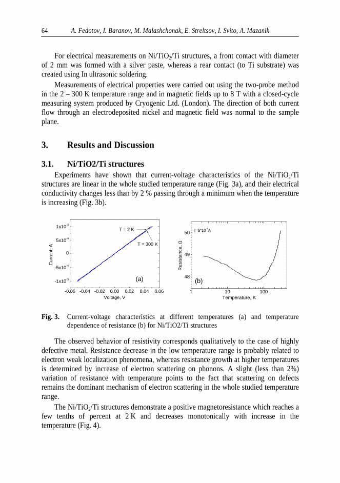
A. Fedotov, I. Baranov, M. Malashchonak, E. Streltsov, I. Svito, A. Mazanik 64
For electrical measurements on Ni/TiO2/Ti structures, a front contact with diameter of 2 mm was formed with a silver paste, whereas a rear contact (to Ti substrate) was created using In ultrasonic soldering.
Measurements of electrical properties were carried out using the two-probe method in the 2 – 300 K temperature range and in magnetic fields up to 8 T with a closed-cycle measuring system produced by Cryogenic Ltd. (London). The direction of both current flow through an electrodeposited nickel and magnetic field was normal to the sample plane.
3. Results and Discussion
3.1. Ni/TiO2/Ti structures Experiments have shown that current-voltage characteristics of the Ni/TiO2/Ti
structures are linear in the whole studied temperature range (Fig. 3a), and their electrical conductivity changes less than by 2 % passing through a minimum when the temperature is increasing (Fig. 3b).
-1x10⁻³
-5x10⁻⁴
0
5x10⁻⁴
1x10⁻³
-0.06 -0.04 -0.02 0.00 0.02 0.04 0.06
(a)
T = 2 K
Voltage, V
Cur
rent
, A
T = 300 K
1 10 100
48
49
50 I=5*10-4A
Res
ista
nce,
Ω
Temperature, K
(b)
Fig. 3. Current-voltage characteristics at different temperatures (a) and temperature
dependence of resistance (b) for Ni/TiO2/Ti structures
The observed behavior of resistivity corresponds qualitatively to the case of highly defective metal. Resistance decrease in the low temperature range is probably related to electron weak localization phenomena, whereas resistance growth at higher temperatures is determined by increase of electron scattering on phonons. A slight (less than 2%) variation of resistance with temperature points to the fact that scattering on defects remains the dominant mechanism of electron scattering in the whole studied temperature range.
The Ni/TiO2/Ti structures demonstrate a positive magnetoresistance which reaches a few tenths of percent at 2 K and decreases monotonically with increase in the temperature (Fig. 4).

Magnetoresistive properties of Ni/TiO2/Ti and Ni/SiO2/Si structures… 65
-8 -6 -4 -2 0 2 4 6 8
0.000
0.002
0.004
0.006
1
2 R
elat
ive
mag
neto
resi
stan
ce
Magnetic field, T
3 - 6
Fig. 4. Magnetoresistance of Ti/TiO2/Ni structure at 2 К (1), 5 К (2), 25 К, 50 К, 150 К,
and 300 К (3 – 6)
3.2. Ni/SiO2/Si structures Current-voltage characteristics of the Ni/SiO2/Si structures measured at different
temperatures in both presence and absence of magnetic field are given in Fig. 5. An asymmetrical shape of I-V curves points to good rectifying properties of the Schottky barrier formed between Ni and Si substrate.
In the whole studied temperature range the formed Ni/SiO2/Si structures demonstrate a positive magnetoresistance, which increases monotonically when the temperature is decreasing (Fig. 6).
-0.2 0.0 0.2 0.4
0
1x10⁻⁷
2x10⁻⁷
3x10⁻⁷
4x10⁻⁷
5x10⁻⁷
2
4
3
Cur
rent
, A
Voltage, V
1
Fig. 5. Current-voltage characteristics of Ni/SiO2/Si structures at 20 K (1,2) and 25 K (3,4) without (1,3) and with magnetic field В = 8 T (2,4)

A. Fedotov, I. Baranov, M. Malashchonak, E. Streltsov, I. Svito, A. Mazanik 66
-8 -4 0 4 8
0.0
0.5
1.0
1.5
U = 2 V U = 5 V U = 10 V
Rel
ativ
e m
agne
tore
sist
ance
Magnetic field, T
Ò = 20 Ê
(a)
-8 -4 0 4 8
0.0
0.2
0.4
0.6 U = 0.05 V U = 0.5 V U = 1 V
Rel
ativ
e m
agne
tore
sist
ance
Magnetic field, T
Ò = 300 Ê
(b)
Fig. 6. Magnetoresistance of Ni/SiO2/Si structure at 20 К (a) and 300 K (b) and different bias
voltages U
As is seen from Figures 4 and 6, magnetoresistance of the Ni/SiO2/Si structures is much higher in comparison with Ni/TiO2/Ti ones indicating that the main contribution to the observed magnetoresistive properties is given by the silicon substrate. The square-low dependence of magnetoresistance on magnetic field may point to its Lorentz nature.
Resume Ni/TiO2/Ti and Ni/SiO2/Si structures have been prepared using electrochemical
deposition of Ni on TiO2 nanotubes and windows in SiO2 layer, respectively. Magnetoresistance of these structures was measured depending on the temperature and magnetic field. The performed experiments have shown that the maximal value of magnetoresistance is achieved in the case of Ni/SiO2/Si structures and reaches about 60 % at room temperature in magnetic field 8 T.
Acknowledgments The work was financially supported by the Research Program “Nanomaterials and
Nanotechnologies” of the Republic of Belarus (contract No 2.4.08).
Bibliography 1. Y. Imry, in: Nanostructures and Mesoscopic Systems, edited by W. P. Kirk and M. A.
Reed, (Academic, New York), p. 11. 1992. 2. Template-based synthesis of nanorod or nanowire arrays. In: Springer Handbook of
nanotechnology. Bharat Brushan (ed.). Springer, pp. 161–178. 2007. 3. A. Fujishima, K. Honda. Electrochemical photolysis of water at a semiconductor
electrode Nature 238, pp. 37–38. 1972.
Magnetoresistive properties of Ni/TiO2/Ti and Ni/SiO2/Si structures… 67
4. Y. Wang, Y. He, Q. Lai, M. Fan. Review of the progress in preparing nano TiO2: An important environmental engineering material Journal of Environmental Sciences 26, pp. 2139–2177. 2014.
5. Q. Zhou, Z. Fang, J. Li, M. Wang. Applications of TiO2 nanotube arrays in environmental and energy fields: A review Microporous and Mesoporous Materials 202, pp. 22–35. 2015.
6. X. Zhou, N.T. Nguyen, S. Özkan, P. Schmuki. Anodic TiO2 nanotube layers: Why does self-organized growth occur – A mini review Electrochemistry Communications 46, pp. 157–162. 2014.
7. Q. Cai, M. Paulose, O.K. Varghese, C.A. Grimes. The effect of electrolyte composition on the fabrication of self-organized titanium oxide nanotube arrays by anodic oxidation Journal of Materials Research 20, pp. 230–236. 2005.
8. S.Yu. Turishchev, E.V. Parinova, F. Kronast, R. Ovsyannikov, N. V. Malashchenok, E. A. Streltsov, D. K. Ivanov, A. K. Fedotov. Photoemission electron microscopy of arrays of submicron nickel rods in a silicon dioxide matrix Physics of the Solid State 56 (9), pp. 1916–1921. 2014.
9. M.V. Malashchonak, A.V. Mazanik, O.V. Korolik, Е.А. Streltsov, A.I. Kulak.
Influence of Wide Band-Gap Oxide Substrate on Photoelectrochemical Properties and Structural Disorder of CdS Nanoparticles Grown by Successive Ionic Layer Adsorption and Reaction (SILAR) Method Beilstein Journal of Nanotechnology (in print).
Abstract Magnetoresistive properties of Ni/TiO2/Ti and Ni/SiO2/Si structures obtained using
template-based approach have been examined in the temperature range from 2 to 300 K. It was established that the main contribution into observed magnetoresistance is given by the silicon substrate, whereas influence of Ni is negligible small.
Streszczenie Właściwości magnetyczne struktur Ni/TiO2/Ti oraz Ni/SiO2/Si otrzymanych
z zastosowaniem tzw. „podejścia szabłonowego” zostały zbadane w zakresie temperatur od 2 do 300 K. Ustalono, że główny wkład do obserwowanej magnetorezystancji jest rezultatem wpływu podłoża krzemowego , podczas gdy wpływ Ni jest znikome mały. Słowa kluczowe: Struktury Ni/TiO2/Ti oraz Ni/SiO2/Si, magnetorezystancja


Igor Troyanchuk Maxim Bushinsky Nina Tereshko Vera Fedotova Scientific-Practical Materials Research Centre of NAS of Belarus Minsk, Belarus
Magnetic and magnetotransport properties of La0.5Sr0.5Co0.8Me0.2O3 (Me=Cr, Fe) cobaltites
Keywords: magnetic interactions; magnetization; magnetoresistance; metal-insulator transition
1. Introduction Perovskite oxides of transition metal ions are of particular interest due to
unusual magnetic and transport properties. Cobaltites of RCoO3 systems (R – rare earth ions) have attracted special attention because of additional degree of freedom provided by different spin configurations. The most known member of this family LaCoO3 has been intensively studied for more than six decades [1-6].
Comparable influence of the intra-atomic Hund’s exchange energy and the crystal field splitting causes a flexibility in spin-states of Co3+ ions in LaCoO3. There are three possible spin states of the cobalt ions with 3d6 configurations - low-spin state with S=0, an intermediate-spin state with S=1 and a high-spin state with S=2.
Besides the extra degree of freedom caused by spin-state flexibility, the substituted cobaltites R1-xAxCoO3 (A – alkali earth ions) have attracted great attention due to other phenomena i.e. a competition between ferromagnetism, antiferromagnetism and cluster-glass ground state, giant magnetoresistance as well as phase separation [1-7]. The origin of the ferromagnetism in the metallic cobaltites remains the subject of discussions for a long time.
It is considered than ferromagnetic coupling between cobalt ions being in 3+ and 4+ oxidation states is coused by double exchange interaction [8]. However some compounds having only homovalent Co ions like SrCoO3, SrFe1-xCoxO3 and LaCo1-
xNixO3 show metallic behavior and ferromagnetism [9-12]. Epitaxially strained LaCoO3 thin films also exhibit long-range ferromagnetic order below 85 K [13].

Igor Troyanchuk, Maxim Bushinsky, Nina Tereshko, Vera Fedotova 70
The available studies do not definitely solve the issue of the origin of magnetic interactions in cobaltites.
The substitution of Co ions can modify the magnetic ordering and facilitate understanding the origin of the ferromagnetic state as well as estimating the spin state of the Co ions. The effect of the substitution of Co ions by Cr ones in La0.5Ba0.5Co1-xCrxO3 system has been studied in Ref. [14] where an increase of the Curie point from 189 K (x = 0) up to 205 K (x = 0.1) has been reported. The change in the Curie point has been attributed to the double exchange interactions between cobalt and chromium ions. In the actual study we declare contrary effect caused by a substitution of cobalt ions by Cr, Fe ones in La0.5Sr0.5Co0.8Me0.2O3 system.
2. Experimental procedures La0.5Sr0.5Co0.8Me0.2O3 (Me = Cr, Fe) ceramics and the parent compound
La0.5Sr0.5CoO3 were prepared by solid state reaction. High purity oxides La2O3, Co3O4, Cr2O3, Fe2O3 and carbonate SrCO3 were taken in stoichiometric ratio and thoroughly mixed in planetary mill Retsch-PM100; the mixture were annealed in air at 1270 K for 10 h. After regrinding, the samples were annealed in air at 1470 – 1600 K for 10 h and slowly cooled at a rate of 15 C/h. Step-scanned powder X-ray diffraction data were recorded at room temperature using DRON-3M diffractometer with Cu-Kα radiation. The diffraction data were analysed by the Rietveld method using the Full Prof software package. The structural data testified a formation of the single phase compounds with perovskite-like structure. The magnetic and transport properties of the samples were investigated using PPMS set-up (Cryogenic Ltd) in magnetic fields up to 14 T and temperature range of 5 – 320 K. Resistivity measurements were carried out using standard four-probe technique.
3. Experimental results The results of X-ray diffraction measurements indicate that all studied samples
are characterized by single phase rhombohedral perovskite structure (space group R-3c). The estimated structure of the parent compound La0.5Sr0.5CoO3 is in agreement with that declared in the earlier reports [15]. The chemical substitution by cobalt ions does not lead to significant modification of the unit cell parameters particularly the bond angle Co – O – Co and the bond length Co – O. Herein, the lattice degree of freedom can be ignored while considering the magnetic and electrical transport behavior for different Cr and Fe doped samples.
Figure 1 shows the magnetization as a function of temperature measured for parent compound and La0.5Sr0.5Co0.8Me0.2O3 (Me = Cr, Fe) solid solutions in magnetic field of 0.01 T. The La0.5Sr0.5CoO3 compound undergoes a paramagnetic to
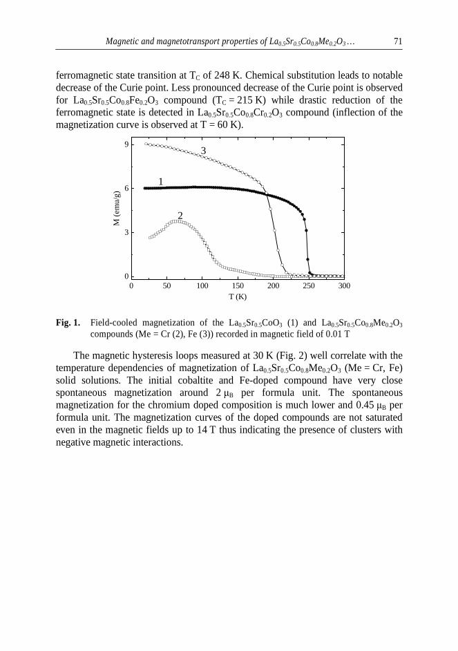
Magnetic and magnetotransport properties of La0.5Sr0.5Co0.8Me0.2O3 … 71
ferromagnetic state transition at TC of 248 K. Chemical substitution leads to notable decrease of the Curie point. Less pronounced decrease of the Curie point is observed for La0.5Sr0.5Co0.8Fe0.2O3 compound (TC = 215 K) while drastic reduction of the ferromagnetic state is detected in La0.5Sr0.5Co0.8Cr0.2O3 compound (inflection of the magnetization curve is observed at T = 60 K).
0 50 100 150 200 250 3000
3
6
9
M (
em
u/g)
T (K)
1
2
3
Fig. 1. Field-cooled magnetization of the La0.5Sr0.5CoO3 (1) and La0.5Sr0.5Co0.8Me0.2O3 compounds (Me = Cr (2), Fe (3)) recorded in magnetic field of 0.01 T
The magnetic hysteresis loops measured at 30 K (Fig. 2) well correlate with the temperature dependencies of magnetization of La0.5Sr0.5Co0.8Me0.2O3 (Me = Cr, Fe) solid solutions. The initial cobaltite and Fe-doped compound have very close spontaneous magnetization around 2 μB per formula unit. The spontaneous magnetization for the chromium doped composition is much lower and 0.45 μB per formula unit. The magnetization curves of the doped compounds are not saturated even in the magnetic fields up to 14 T thus indicating the presence of clusters with negative magnetic interactions.
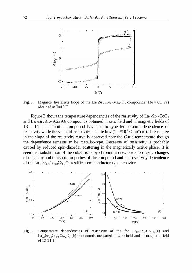
Igor Troyanchuk, Maxim Bushinsky, Nina Tereshko, Vera Fedotova 72
-15 -10 -5 0 5 10 15
-2
-1
0
1
2
M (
µ B/f.
u.)
B (T)
1
3
2
Fig. 2. Magnetic hysteresis loops of the La0.5Sr0.5Co0.8Me0.2O3 compounds (Me = Cr, Fe) obtained at T=10 K
Figure 3 shows the temperature dependencies of the resistivity of La0.5Sr0.5CoO3 and La0.5Sr0.5Co0.8Cr0.2O3 compounds obtained in zero field and in magnetic fields of 13 – 14 T. The initial compound has metallic-type temperature dependence of resistivity while the value of resistivity is quite low (1-2*10-4 Ohm*cm). The change in the slope of the resistivity curve is observed near the Curie temperature though the dependence remains to be metallic-type. Decrease of resistivity is probably caused by reduced spin-disorder scattering in the magnetically active phase. It is seen that substitution of the cobalt ions by chromium ones leads to drastic changes of magnetic and transport properties of the compound and the resistivity dependence of the La0.5Sr0.5Co0.8Cr0.2O3 testifies semiconductor-type behavior.
0 50 100 150 200 250 3000.6
1.2
1.8
2.4
T (K)
B=14T
B=0T
ρ·10
-4
(Ω·c
m)
(a)
0 50 100 150 200 250 300
20
40
60
80
100
(b)B=13T
B=0T
ρ·1
0-4 (
Ω·c
m)
T (K)
Fig. 3. Temperature dependencies of resistivity of the for La0.5Sr0.5CoO3 (a) and La0.5Sr0.5Co0.8Cr0.2O3 (b) compounds measured in zero-field and in magnetic field of 13-14 T.
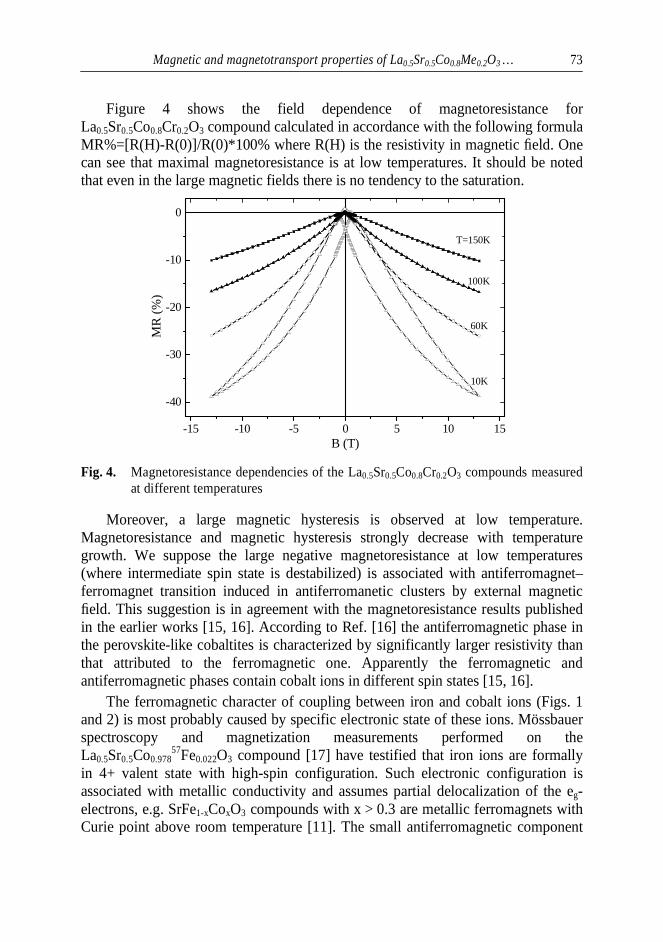
Magnetic and magnetotransport properties of La0.5Sr0.5Co0.8Me0.2O3 … 73
Figure 4 shows the field dependence of magnetoresistance for La0.5Sr0.5Co0.8Cr0.2O3 compound calculated in accordance with the following formula MR%=[R(H)-R(0)]/R(0)*100% where R(H) is the resistivity in magnetic field. One can see that maximal magnetoresistance is at low temperatures. It should be noted that even in the large magnetic fields there is no tendency to the saturation.
-15 -10 -5 0 5 10 15
-40
-30
-20
-10
0
10K
60K
100K
MR
(%
)
B (T)
T=150K
Fig. 4. Magnetoresistance dependencies of the La0.5Sr0.5Co0.8Cr0.2O3 compounds measured at different temperatures
Moreover, a large magnetic hysteresis is observed at low temperature. Magnetoresistance and magnetic hysteresis strongly decrease with temperature growth. We suppose the large negative magnetoresistance at low temperatures (where intermediate spin state is destabilized) is associated with antiferromagnet–ferromagnet transition induced in antiferromanetic clusters by external magnetic field. This suggestion is in agreement with the magnetoresistance results published in the earlier works [15, 16]. According to Ref. [16] the antiferromagnetic phase in the perovskite-like cobaltites is characterized by significantly larger resistivity than that attributed to the ferromagnetic one. Apparently the ferromagnetic and antiferromagnetic phases contain cobalt ions in different spin states [15, 16].
The ferromagnetic character of coupling between iron and cobalt ions (Figs. 1 and 2) is most probably caused by specific electronic state of these ions. Mössbauer spectroscopy and magnetization measurements performed on the La0.5Sr0.5Co0.978
57Fe0.022O3 compound [17] have testified that iron ions are formally in 4+ valent state with high-spin configuration. Such electronic configuration is associated with metallic conductivity and assumes partial delocalization of the eg-electrons, e.g. SrFe1-xCoxO3 compounds with x > 0.3 are metallic ferromagnets with Curie point above room temperature [11]. The small antiferromagnetic component

Igor Troyanchuk, Maxim Bushinsky, Nina Tereshko, Vera Fedotova 74
(Fig. 1 and 2) is most probably associated with Fe3+-enriched clusters while the superexchange interactions between Co3+ and Fe3+ ions are strongly antiferromagnetic [18]. The magnetization and the Curie point of chromium doped sample are minimal among the considered compounds (Figs. 1 and 2). This is probably caused by strong antiferromagnetic coupling between chromium and cobalt ions. The antiferromagnetic type of the interactions between chromium and cobalt ions points on the dominance of superexchange interactions as the double exchange interaction lead to ferromagnetic coupling.
4. Summary Magnetic and magnetotransport properties of La0.5Sr0.5Co0.8Me0.2O3 (Me = Cr,
Fe) perovskite-like cobaltites with stoichiometric compositions were studied. It is shown that the substitution with Fe ions does not strongly affect spontaneous magnetization and the Curie point. In contrast, chromium substitution leads to dramatic decrease of magnetization, Curie point and strongly modifies the temperature dependence of magnetization. The magnetization data are discussed assuming positive magnetic interactions between Co and Fe ions, while magnetic interactions between Co and Cr are considered to be negative. Substitution of Co by Cr ions strongly increases magnetoresistance at low temperature and causes metal-insulator transition. Drastic increase of magnetoresistance seems to be caused by antiferromagnet-ferromagnet transition induced by strong magnetic field.
Acknowledgments This work is supported by the Belarusian Republican Foundation for
Fundamental Research (Project F14R-040).
References 1. Jonker G.H., Van Santen J.H., Magnetic compounds with perovskite structure.
III. Ferromagnetic compounds of cobalt, Physica 19 (1953), 120-130 2. Raccah P.M., Goodenough J.B. First-Order Localized-Electron Collective-
Electron Transition in LaCoO3, Phys. Rev. 155 (1967), No. 3, 932-943 3. B. Raveau, M.M. Seikh, Cobalt Oxides: From Crystal Chemistry to Physics,
Wiley-VCH Verlag GmbH & Co. KGaA, Weinheim, 2012. 148 4. J.B. Goodenough, J.S. Zhou, in Structure and Bonding, Springer, New York,
2001, pp. 17-113 5. Fauth F., Suard E., Caignaert V., Intermediate spin state of Co3+ and Co4+ ions in
La0.5Ba0.5CoO3 evidenced by Jahn-Teller distortions, Phys. Rev. B 65 (2001), No. 6, 060401(R)

Magnetic and magnetotransport properties of La0.5Sr0.5Co0.8Me0.2O3 … 75
6. Fita I., Szymczak R., Puzniak R., Wisniewski A., Troyanchuk I.O., Karpinsky D.V., Markovich V., Szymczak H., Ferromagnetic state of La1−xBaxCoO3 under applied pressure: Factors controlling the sign reversal of pressure effect in cobaltites, Phys. Rev. B 83 (2011), No. 6, 064414
7. Yan J.Q., Zhou J.S., Goodenough J.B., Bond-length fluctuations and the spin-state transition in LCoO3 (L=La, Pr, and Nd), Phys. Rev. B 69 (2004), No. 13, 134409
8. Wu J., Leighton C., Glassy ferromagnetism and magnetic phase separation in La1−xSrxCoO3, Phys. Rev. B 67 (2003), No. 17, 174408
9. Zener C., Interaction between the d-Shells in the Transition Metals. II. Ferromagnetic Compounds of Manganese with Perovskite Structure, Phys. Rev. 82 (1951), No. 3, 403-405
10. Long Y., Kaneko Y., Ishiwata S., Taguchi Y., Tokura Y., Synthesis of cubic SrCoO3 single crystal and its anisotropic magnetic and transport properties, J. Phys.: Cond. Matter 23 (2011), No. 24, 245601
11. Yin C., Liu Q., Decourt R., Pollet M., Gaudin E., Toulemonde O., Unusual oxidation states give reversible room temperature magnetocaloric effect on perovskite-related oxides SrFe0.5Co0.5O3, J. Sol. State Chem. 184 (2011), No. 12, 3228-3231
12. Blasco J., García J., Magnetic properties of NdNi1−xCoxO3 samples: Evidence of spin-glass behavior, Phys. Rev. B 51 (1995), No. 6, 3569-3574
13. Rivadulla F., Bi Z., Bauer E., Rivas-Murias B., Vila-Fungueiriño J.M., Jia Q., Strain-Induced Ferromagnetism and Magnetoresistance in Epitaxial Thin Films of LaCoO3 Prepared by Polymer-Assisted Deposition, Chem. Mater. 25 (2013), No. 1, 55-58
14. Zhang S., Pi L., Tong W., Tan S., Zhang C., Zhang Y., Cr enhanced ferromagnetism in La0.5Ba0.5CoO3 due to possible double-exchange interaction, J. Alloys Compd. 628 (2015), 251–256
15. Karpinsky D.V., Troyanchuk I.O., Lobanovsky L.S., Chobot A.N., Ritter C., Efimov V., Sikolenko V., Kholkin A.L., Magnetic and structural phase transitions in La0.5Sr0.5CoO3−δ (0≤δ<0.3) cobaltites, J. Phys.: Cond. Matter 25 (2013), No. 31, 316004
16. Troyanchuk I.O., Bushinsky M.V., Nikitin A.V., Lobanovsky L.S., Balagurov A.M., Sikolenko V., Efimov V., Sheptyakov D.V., Very large magnetoresistance and spin state transition in Ba-doped cobaltites, J. Appl. Phys. 113 (2013), No. 5, 053909
17. Kopcewicz M., Karpinsky D.V., Troyanchuk I.O., Mössbauer study of 57Fe-doped La0.5Sr0.5CoO3, J. Phys.: Cond. Matter 17 (2005), No. 48, 7743

Igor Troyanchuk, Maxim Bushinsky, Nina Tereshko, Vera Fedotova 76
18. Troyanchuk I.O., Karpinsky D.V., Yokaichiya F. Effect of iron doping on the magnetic structure of TbBaCo2O5.5 layered perovskite, J. Phys.: Condens. Matter 20 (2008), No. 33 , 335228.
Abstract Magnetic and magnetotransport properties of La0.5Sr0.5Co0.8Me0.2O3 (Me = Cr,
Fe) stoichiometric cobaltites has been investigated in magnetic fields up to 14 T. It is shown that doping with Fe ions changes spontaneous magnetization only slightly herewith the Curie point significantly decreases. The chromium doping leads to dramatic decrease of magnetization and the Curie point and a strong increase in magnetoresistance at low temperature. The obtained results indicate that the magnetic interactions between Co and Fe are positive whereas those between Co and Cr ions are negative. Enhancement of magnetoresistance is attributed to the magnetic field induced transition from antiferromagnetic order to ferromagnetic one.
Streszczenie Właściwości magnetyczne i magnetotransportowe stoichiometrycznych
kobaltytów zbadano w polach magnetycznych do 14T. Ustalono, że domieszkowanie przez jony Fe zmienia namagnesowanie spontaniczne bardzo słabo w tym czasie jak punkt Curie obniża się znacząco. Domieszkowanie przez atomy chromu powoduje dramatyczne zmniejszenie namagnesowania i obniżenie punktu Curie i mocny wzrost magneto rezystancji w niskich temperaturach. Otrzymane rezultaty wskazują oddziaływanie magnetyczne pomiędzy Co i Fe jest pozytywne w tym czasie jak pomiędzy Co a Cr jest negatywne.
Wzmocnienie magnetorezystancji przypisano do pola magnetycznego indukowanego przejściem z antyferromagnetycznego układu do ferromagnetycznego.
Słowa kluczowe: Oddziaływania magnetyczne; namagnesowanie; magnetorezystancja; przejście metal-izolator
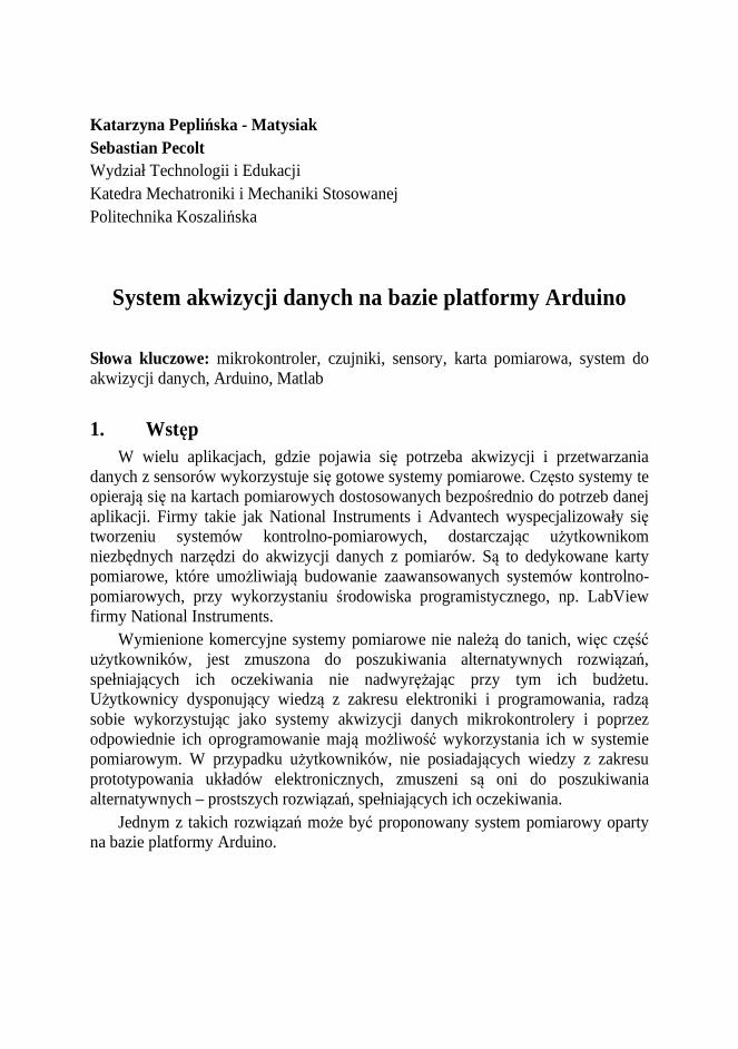
Katarzyna Peplińska - Matysiak Sebastian Pecolt Wydział Technologii i Edukacji Katedra Mechatroniki i Mechaniki Stosowanej Politechnika Koszalińska
System akwizycji danych na bazie platformy Arduino
Słowa kluczowe: mikrokontroler, czujniki, sensory, karta pomiarowa, system do akwizycji danych, Arduino, Matlab
1. Wstęp W wielu aplikacjach, gdzie pojawia się potrzeba akwizycji i przetwarzania
danych z sensorów wykorzystuje się gotowe systemy pomiarowe. Często systemy te opierają się na kartach pomiarowych dostosowanych bezpośrednio do potrzeb danej aplikacji. Firmy takie jak National Instruments i Advantech wyspecjalizowały się tworzeniu systemów kontrolno-pomiarowych, dostarczając użytkownikom niezbędnych narzędzi do akwizycji danych z pomiarów. Są to dedykowane karty pomiarowe, które umożliwiają budowanie zaawansowanych systemów kontrolno-pomiarowych, przy wykorzystaniu środowiska programistycznego, np. LabView firmy National Instruments.
Wymienione komercyjne systemy pomiarowe nie należą do tanich, więc część użytkowników, jest zmuszona do poszukiwania alternatywnych rozwiązań, spełniających ich oczekiwania nie nadwyrężając przy tym ich budżetu. Użytkownicy dysponujący wiedzą z zakresu elektroniki i programowania, radzą sobie wykorzystując jako systemy akwizycji danych mikrokontrolery i poprzez odpowiednie ich oprogramowanie mają możliwość wykorzystania ich w systemie pomiarowym. W przypadku użytkowników, nie posiadających wiedzy z zakresu prototypowania układów elektronicznych, zmuszeni są oni do poszukiwania alternatywnych – prostszych rozwiązań, spełniających ich oczekiwania.
Jednym z takich rozwiązań może być proponowany system pomiarowy oparty na bazie platformy Arduino.
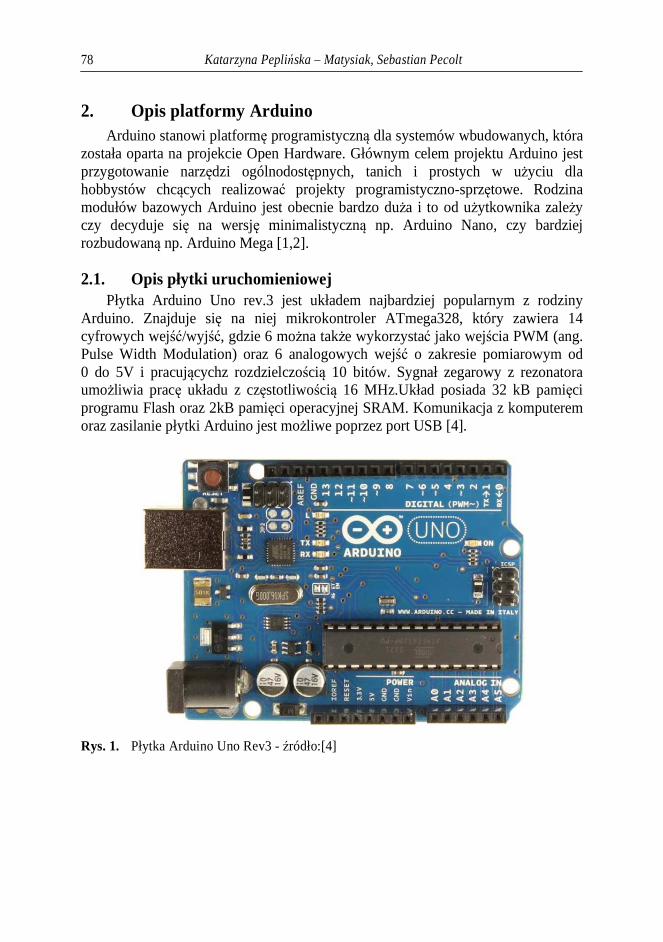
Katarzyna Peplińska – Matysiak, Sebastian Pecolt 78
2. Opis platformy Arduino Arduino stanowi platformę programistyczną dla systemów wbudowanych, która
została oparta na projekcie Open Hardware. Głównym celem projektu Arduino jest przygotowanie narzędzi ogólnodostępnych, tanich i prostych w użyciu dla hobbystów chcących realizować projekty programistyczno-sprzętowe. Rodzina modułów bazowych Arduino jest obecnie bardzo duża i to od użytkownika zależy czy decyduje się na wersję minimalistyczną np. Arduino Nano, czy bardziej rozbudowaną np. Arduino Mega [1,2].
2.1. Opis płytki uruchomieniowej Płytka Arduino Uno rev.3 jest układem najbardziej popularnym z rodziny
Arduino. Znajduje się na niej mikrokontroler ATmega328, który zawiera 14 cyfrowych wejść/wyjść, gdzie 6 można także wykorzystać jako wejścia PWM (ang. Pulse Width Modulation) oraz 6 analogowych wejść o zakresie pomiarowym od 0 do 5V i pracującychz rozdzielczością 10 bitów. Sygnał zegarowy z rezonatora umożliwia pracę układu z częstotliwością 16 MHz.Układ posiada 32 kB pamięci programu Flash oraz 2kB pamięci operacyjnej SRAM. Komunikacja z komputerem oraz zasilanie płytki Arduino jest możliwe poprzez port USB [4].
Rys. 1. Płytka Arduino Uno Rev3 - źródło:[4]
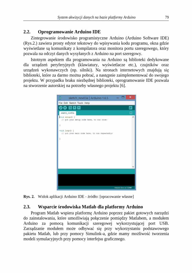
System akwizycji danych na bazie platformy Arduino 79
2.2. Oprogramowanie Arduino IDE Zintegrowanie środowisko programistyczne Arduino (Arduino Software IDE)
(Rys.2.) zawiera prosty edytor tekstowy do wpisywania kodu programu, okna gdzie wyświetlane są komunikaty z kompilatora oraz monitora portu szeregowego, który pozwala na odczyt danych wysyłanych z Arduino na port szeregowy.
Istotnym aspektem dla programowania na Arduino są biblioteki dedykowane dla urządzeń peryferyjnych (klawiatury, wyświetlacze etc.), czujników oraz urządzeń wykonawczych (np. silniki). Na stronach internetowych znajdują się biblioteki, które za darmo można pobrać, a następnie zaimplementować do swojego projektu. W przypadku braku niezbędnej biblioteki, oprogramowanie IDE pozwala na stworzenie autorskiej na potrzeby własnego projektu [6].
Rys. 2. Widok aplikacji Arduino IDE - źródło: [opracowanie własne]
2.3. Wsparcie środowiska Matlab dla platformy Arduino Program Matlab wspiera platformę Arduino poprzez pakiet gotowych narzędzi
do zainstalowania, które umożliwiają połączenie pomiędzy Matlabem, a modułem Arduino za pomocą komunikacji szeregowej wykorzystującej port USB. Zarządzanie modułem może odbywać się przy wykorzystaniu podstawowego pakietu Matlab, lub przy pomocy Simulink-a, gdzie mamy możliwość tworzenia modeli symulacyjnych przy pomocy interfejsu graficznego.
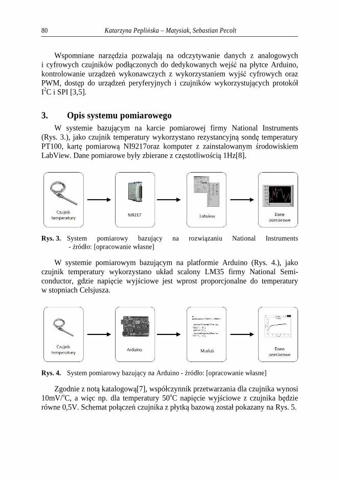
Katarzyna Peplińska – Matysiak, Sebastian Pecolt 80
Wspomniane narzędzia pozwalają na odczytywanie danych z analogowych i cyfrowych czujników podłączonych do dedykowanych wejść na płytce Arduino, kontrolowanie urządzeń wykonawczych z wykorzystaniem wyjść cyfrowych oraz PWM, dostęp do urządzeń peryferyjnych i czujników wykorzystujących protokół I2C i SPI [3,5].
3. Opis systemu pomiarowego W systemie bazującym na karcie pomiarowej firmy National Instruments
(Rys. 3.), jako czujnik temperatury wykorzystano rezystancyjną sondę temperatury PT100, kartę pomiarową NI9217oraz komputer z zainstalowanym środowiskiem LabView. Dane pomiarowe były zbierane z częstotliwością 1Hz[8].
Rys. 3. System pomiarowy bazujący na rozwiązaniu National Instruments - źródło: [opracowanie własne]
W systemie pomiarowym bazującym na platformie Arduino (Rys. 4.), jako czujnik temperatury wykorzystano układ scalony LM35 firmy National Semi-conductor, gdzie napięcie wyjściowe jest wprost proporcjonalne do temperatury w stopniach Celsjusza.
Rys. 4. System pomiarowy bazujący na Arduino - źródło: [opracowanie własne]
Zgodnie z notą katalogową[7], współczynnik przetwarzania dla czujnika wynosi 10mV/oC, a więc np. dla temperatury 50oC napięcie wyjściowe z czujnika będzie równe 0,5V. Schemat połączeń czujnika z płytką bazową został pokazany na Rys. 5.

System akwizycji danych na bazie platformy Arduino 81
Rys. 5. Schemat połączenia czujnika temperatury z modułem Arduino - źródło: [opracowanie własne z wykorzystaniem programu Fritzing]
Program do odczytywania napięcia z czujnika temperatury w wyznaczonych chwilach czasu, tj. co jedną sekundę wysyła żądanie do Arduino o podanie napięcia z portu, do którego jest podłączony czujnik, a następnie zapisuje w przestrzeni roboczej Matlaba wraz z informacją o czasie w którym próbka została zebrana. Kod programu do akwizycji danych został napisany w m-pliku w środowisku Matlab.
W związku z tym, że w systemie pomiarowym powstają niewielkie opóźnienia związane z wysłaniem żądania poprzez port USB i odebraniem danych, system taki nie sprawdzi się w zastosowaniach, gdzie wymagana jest duża częstotliwość próbkowania. Z przeprowadzonych badań wynika, że opóźnienie związane z odczytem wartości waha się w granicach 30ms, co w przypadku opisywanego systemu do monitorowania temperatury nie wpływa negatywnie na proces akwizycji danych.
4. Wyniki pomiarów Proces, w którym były wykorzystywane systemy pomiarowe, dotyczył
podgrzewania wody w zbiorniku wodnym z grzałką elektryczną. Danymi pomiarowymi, były temperatura wody w funkcji czasu. Stanowisko pomiarowe zostało zestawione zgodnie z Rys. 6. Wykorzystane w badaniu czujniki temperatury zostały umieszczone wewnątrz zbiornika wodnego. Wodę podgrzewano od temperatury początkowej tj. 16,5°C do temperatury wrzenia wody.
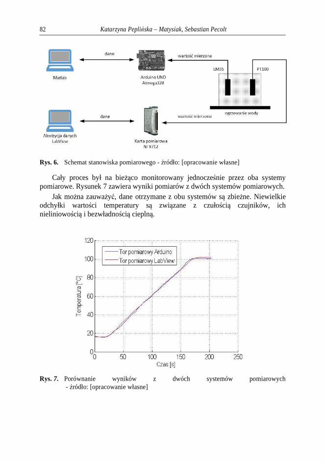
Katarzyna Peplińska – Matysiak, Sebastian Pecolt 82
Rys. 6. Schemat stanowiska pomiarowego - źródło: [opracowanie własne]
Cały proces był na bieżąco monitorowany jednocześnie przez oba systemy pomiarowe. Rysunek 7 zawiera wyniki pomiarów z dwóch systemów pomiarowych.
Jak można zauważyć, dane otrzymane z obu systemów są zbieżne. Niewielkie odchyłki wartości temperatury są związane z czułością czujników, ich nieliniowością i bezwładnością cieplną.
Rys. 7. Porównanie wyników z dwóch systemów pomiarowych - źródło: [opracowanie własne]

System akwizycji danych na bazie platformy Arduino 83
5. Posumowanie Zaprezentowany system pomiarowy na bazie platformy Arduino stanowi
ciekawą alternatywę dla komercyjnych systemów pomiarowych. Z uwagi na popularność środowiska do obliczeń naukowych Matlab na uczelniach wyższych wśród studentów oraz biorąc pod uwagę prostotę implementacji sprzętowej, system taki może mieć zastosowanie w wielu aplikacjach niewymagających wysokiej częstotliwości próbkowania sygnału mierzonego. Wykorzystywane w systemie pomiarowym Arduino oprogramowanie Matlab, nie jest tanie dla przeciętnego użytkownika, jednak jest to środowisko dostępne dla studentów w niemal każdej uczelni. Aby wykluczyć koszt używanego oprogramowania, program Matlab może być z powodzeniem zastąpiony darmowym oprogramowaniem Scilab, które jest także rozbudowanym środowiskiem do obliczeń naukowych, wspierającym platformę Arduino. Wówczas koszt realizacji systemu pomiarowego, sprowadza się jedynie do zakupu wybranej wersji modułu Arduino i odrobiny pracy związanej z napisaniem programu do akwizycji danych.
Bibliografia 1. Monk S.: Arduino dla początkujących. Podstawy i szkice, ISBN 978-83-246-
8707-7, Wydawnictwo Helion 2014 2. Evans M., Noble J., Hochenbaum J.: Arduino w akcji, ISBN: 978-83-246-6356-
9, Wydawnictwo Helion 2014 3. Mrozek B., Mrozek Z.: MATLAB i Simulink poradnik użytkownika, ISBN: 978-
83-246-2564-2, Helion 2010 4. Botland [online], http://botland.com.pl/, data dostępu 21.10.2015 5. Matlab [online],http://www.mathworks.com/, data dostępu 28.10.2015 6. Arduino [online], https://www.arduino.cc/, data dostępu 28.10.2015 7. Texas Instrumenst, LM35 Precision Centigrade Temperature Sensors,
SNIS159E. 8. National Instruments [online], http://www.ni.com/datasheet/pdf/en/ds-193, data
dostępu 04.11.2015

Katarzyna Peplińska – Matysiak, Sebastian Pecolt 84
Abstract The article presents a data acquisition and measurement system based on
Arduino. It includes a design and implementation based on prototype module Arduino Uno rev 3, which is supported by Matlab for scientific and engineering calculation.
Second part of the article is dedicated to comparison of mentioned system with a commercial solution based on National Instruments hardware and it presents advantages and disadvantages of both solutions.
Streszczenie Artykuł przedstawia budowę systemu pomiarowego do akwizycji danych, na
bazie platformy Arduino i zawiera realizację przykładowego rozwiązania konstrukcyjnego i programowego opartego na module prototypowym Arduino Uno rev.3, współpracującego ze środowiskiem do obliczeń naukowych i inżynierskich Matlab.
W pracy porównano wyniki pomiarowe z przykładowego procesu grzewczego dla proponowanego systemu akwizycji danych na bazie Arduino i komercyjnego systemu pomiarowego na bazie karty i oprogramowania firmy National Instruments oraz przedstawiono ich wady i zalety.

Mariusz Miziołek Wydział Technologii i Edukacji Politechnika Koszalińska
Algorytm i implementacja protokołu komunikacyjnego MODBUS w środowisku sterownika PLC firmy IDEC
oraz języku programowania C#
Słowa kluczowe: mikrokontroler, PLC, C#, modbus, protokół komunikacyjny, automatyka przemysłowa, IDEC
1. Wstęp W przemyśle oraz w życiu codziennym coraz więcej urządzeń komunikuję się
ze sobą w celu uzyskania dodatkowych informacji o swoim działaniu lub uzyskania kolejnych poleceń do wykonania. W automatyce przemysłowej istnieje wiele standardów komunikacji ale jednym z najstarszych i najczęściej implementowanych jest MODBUS [1], który posiada dwie najpopularniejsze wersje dla portu szeregowego MODBUS RTU oraz dla sieci Ethernet MODBUS TCP.
Przedstawiony w artykule projekt dotyczy istniejącego rozwiązania protokołu komunikacyjnego MODBUS RTU zaimplementowanego w sterowniku PLC firmy IDEC [2]. Prezentowana praca porusza temat realizacji części algorytmu do budowy zapytania oraz analizy odpowiedzi uzyskanej od sterownika PLC firmy IDEC, przy użyciu języka programowania C# [3]. Zapotrzebowanie na wyżej wymieniony algorytm pojawiło się w trakcie realizacji projektu aplikacji do harmonogramowania procesu azotowania w piecu firmy REMIX znajdującym się w Instytucie Technologii Eksploatacji - PIB w Radomiu. Aplikacja (Rys. 1) wymagała umożliwienia połączenia ze sterownikiem PLC w celu nadzorowania procesu azotowania oraz akwizycji danych procesowych uzyskiwanych w jego trakcie.
W kolejnych punktach określono podstawowe warunki i założenia odnośnie algorytmu dla takiego systemu.
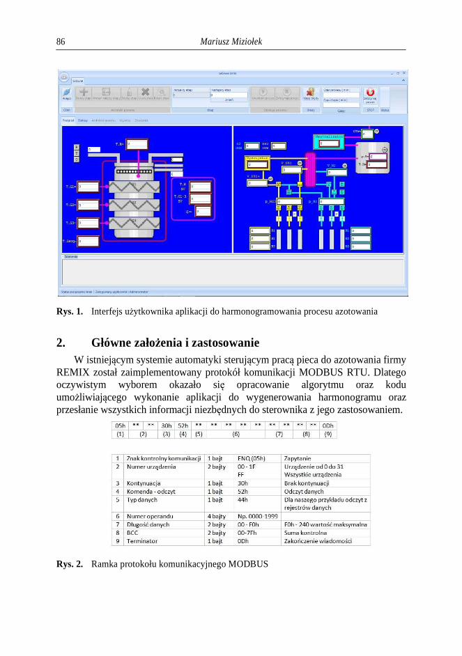
Mariusz Miziołek 86
Rys. 1. Interfejs użytkownika aplikacji do harmonogramowania procesu azotowania
2. Główne założenia i zastosowanie W istniejącym systemie automatyki sterującym pracą pieca do azotowania firmy
REMIX został zaimplementowany protokół komunikacji MODBUS RTU. Dlatego oczywistym wyborem okazało się opracowanie algorytmu oraz kodu umożliwiającego wykonanie aplikacji do wygenerowania harmonogramu oraz przesłanie wszystkich informacji niezbędnych do sterownika z jego zastosowaniem.
Rys. 2. Ramka protokołu komunikacyjnego MODBUS
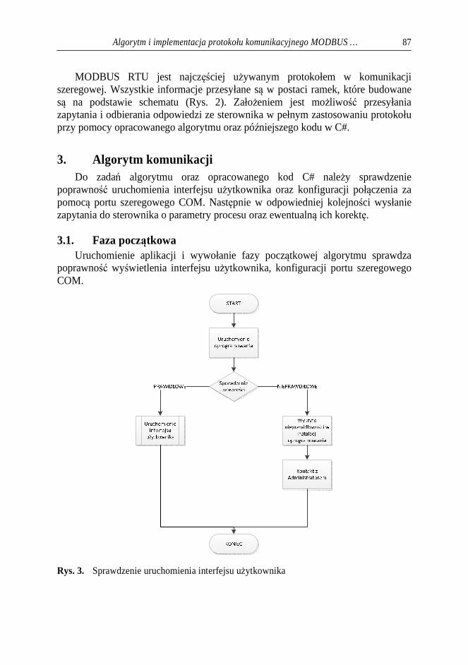
Algorytm i implementacja protokołu komunikacyjnego MODBUS … 87
MODBUS RTU jest najczęściej używanym protokołem w komunikacji szeregowej. Wszystkie informacje przesyłane są w postaci ramek, które budowane są na podstawie schematu (Rys. 2). Założeniem jest możliwość przesyłania zapytania i odbierania odpowiedzi ze sterownika w pełnym zastosowaniu protokołu przy pomocy opracowanego algorytmu oraz późniejszego kodu w C#.
3. Algorytm komunikacji Do zadań algorytmu oraz opracowanego kod C# należy sprawdzenie
poprawność uruchomienia interfejsu użytkownika oraz konfiguracji połączenia za pomocą portu szeregowego COM. Następnie w odpowiedniej kolejności wysłanie zapytania do sterownika o parametry procesu oraz ewentualną ich korektę.
3.1. Faza początkowa Uruchomienie aplikacji i wywołanie fazy początkowej algorytmu sprawdza
poprawność wyświetlenia interfejsu użytkownika, konfiguracji portu szeregowego COM.
Rys. 3. Sprawdzenie uruchomienia interfejsu użytkownika
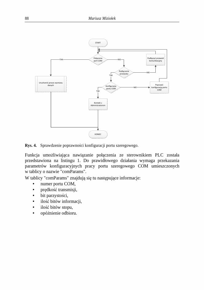
Mariusz Miziołek 88
START
Połączono
port COM
Konfiguracja
portu COM
Podłączenie
przewodu
NIEPodłączyć przewód
komunikacyjny
NIE
TAK
Poprawić
konfigurację portu
COM
NIE
KONIEC
Kontakt z
Administratorem
TAK
Uruchomić proces wymiany
danych
TAK
Rys. 4. Sprawdzenie poprawności konfiguracji portu szeregowego.
Funkcja umożliwiająca nawiązanie połączenia ze sterownikiem PLC została przedstawiona na listingu 1. Do prawidłowego działania wymaga przekazania parametrów konfiguracyjnych pracy portu szeregowego COM umieszczonych w tablicy o nazwie "comParams". W tablicy "comParams" znajdują się tu następujące informacje:
• numer portu COM, • prędkość transmisji, • bit parzystości, • ilość bitów informacji, • ilość bitów stopu, • opóźnienie odbioru.
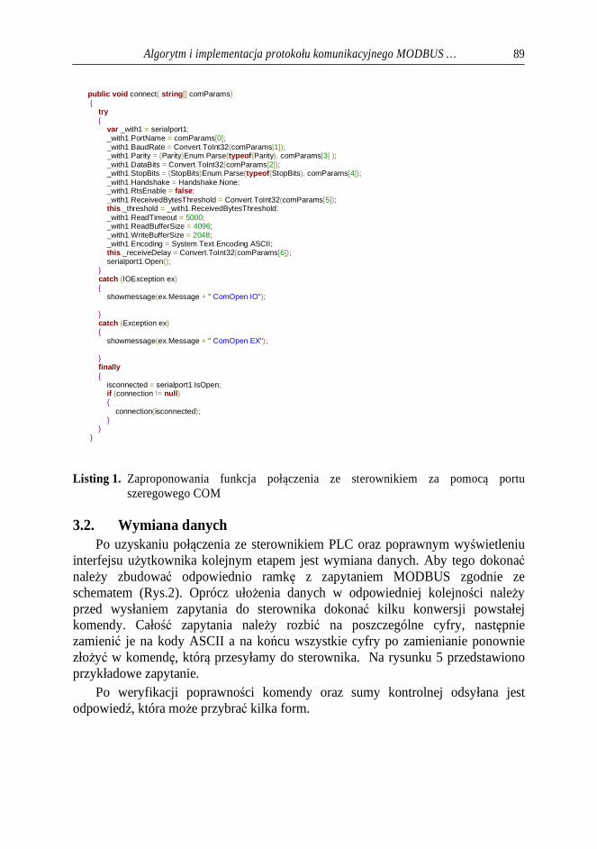
Algorytm i implementacja protokołu komunikacyjnego MODBUS … 89
public void connect( string[] comParams) try var _with1 = serialport1; _with1.PortName = comParams[0]; _with1.BaudRate = Convert.ToInt32(comParams[1]); _with1.Parity = (Parity)Enum.Parse(typeof(Parity), comParams[3] ); _with1.DataBits = Convert.ToInt32(comParams[2]); _with1.StopBits = (StopBits)Enum.Parse(typeof(StopBits), comParams[4]); _with1.Handshake = Handshake.None; _with1.RtsEnable = false; _with1.ReceivedBytesThreshold = Convert.ToInt32(comParams[5]); this._threshold = _with1.ReceivedBytesThreshold; _with1.ReadTimeout = 5000; _with1.ReadBufferSize = 4096; _with1.WriteBufferSize = 2048; _with1.Encoding = System.Text.Encoding.ASCII; this._receiveDelay = Convert.ToInt32(comParams[6]); serialport1.Open(); catch (IOException ex) showmessage(ex.Message + " ComOpen IO"); catch (Exception ex) showmessage(ex.Message + " ComOpen EX"); finally isconnected = serialport1.IsOpen; if (connection != null) connection(isconnected);
Listing 1. Zaproponowania funkcja połączenia ze sterownikiem za pomocą portu szeregowego COM
3.2. Wymiana danych Po uzyskaniu połączenia ze sterownikiem PLC oraz poprawnym wyświetleniu
interfejsu użytkownika kolejnym etapem jest wymiana danych. Aby tego dokonać należy zbudować odpowiednio ramkę z zapytaniem MODBUS zgodnie ze schematem (Rys.2). Oprócz ułożenia danych w odpowiedniej kolejności należy przed wysłaniem zapytania do sterownika dokonać kilku konwersji powstałej komendy. Całość zapytania należy rozbić na poszczególne cyfry, następnie zamienić je na kody ASCII a na końcu wszystkie cyfry po zamienianie ponownie złożyć w komendę, którą przesyłamy do sterownika. Na rysunku 5 przedstawiono przykładowe zapytanie.
Po weryfikacji poprawności komendy oraz sumy kontrolnej odsyłana jest odpowiedź, która może przybrać kilka form.
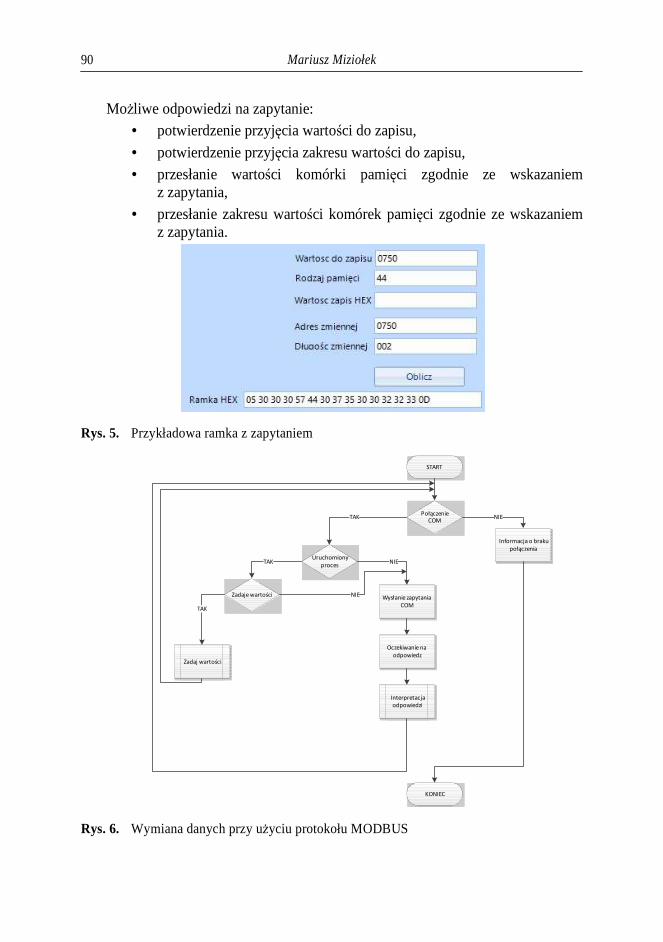
Mariusz Miziołek 90
Możliwe odpowiedzi na zapytanie: • potwierdzenie przyjęcia wartości do zapisu,
• potwierdzenie przyjęcia zakresu wartości do zapisu,
• przesłanie wartości komórki pamięci zgodnie ze wskazaniem z zapytania,
• przesłanie zakresu wartości komórek pamięci zgodnie ze wskazaniem z zapytania.
Rys. 5. Przykładowa ramka z zapytaniem
START
KONIEC
Połączenie
COM
Informacja o braku
połączenia
NIE
Wysłanie zapytania
COM
Oczekiwanie na
odpowiedz
Interpretacja
odpowiedzi
Uruchomiony
proces
TAK
NIE
Zadaje wartości
TAK
NIE
Zadaj wartości
TAK
Rys. 6. Wymiana danych przy użyciu protokołu MODBUS

Algorytm i implementacja protokołu komunikacyjnego MODBUS … 91
private void Oblicz_Click(object sender, EventArgs e) adres0 = Convert.ToChar(TadresZmiennej.Text.Substring(0, 1)); adres1 = Convert.ToChar(TadresZmiennej.Text.Substring(1, 1)); adres2 = Convert.ToChar(TadresZmiennej.Text.Substring(2, 1)); adres3 = Convert.ToChar(TadresZmiennej.Text.Substring(3, 1)); dlugosc0 = Convert.ToInt32(TdlugoscZmiennej.Text); string dlugosc = ""; string HexA0 = ((int)adres0).ToString("X"); string HexA1 = ((int)adres1).ToString("X"); string HexA2 = ((int)adres2).ToString("X"); string HexA3 = ((int)adres3).ToString("X"); string HexD1 = ""; string HexD2 = ""; string HexXOR1 = ""; string HexXOR2 = ""; if (dlugosc0 < 15) char czlon1 = '0'; char czlon2 = Convert.ToChar(dlugosc0.ToString("X")); HexD1 = ((int)czlon1).ToString("X"); HexD2 = ((int)czlon2).ToString("X"); else string HexDlugosc = dlugosc0.ToString("X"); char czlon1 = Convert.ToChar(HexDlugosc.Substring(0, 1)); char czlon2 = Convert.ToChar(HexDlugosc.Substring(1, 1)); HexD1 = ((int)czlon1).ToString("X"); HexD2 = ((int)czlon2).ToString("X"); int czesc1 = Convert.ToInt32("05", 16) ^ Convert.ToInt32("30", 16) ^ Convert.ToInt32("30", 16) ^ Convert.ToInt32("30", 16); int czesc2 = czesc1 ^ Convert.ToInt32("52", 16) ^ Convert.ToInt32(TrodzajPamieci.Text, 16) ^ Convert.ToInt32(HexA0, 16) ^ Convert.ToInt32(HexA1, 16); int czesc3 = czesc2 ^ Convert.ToInt32(HexA2, 16) ^ Convert.ToInt32(HexA3, 16) ^ Convert.ToInt32(HexD1, 16) ^ Convert.ToInt32(HexD2, 16); string hexResult = czesc3.ToString("X"); if (czesc3 > 15) char Xor1 = Convert.ToChar(hexResult.Substring(0, 1)); char Xor2 = Convert.ToChar(hexResult.Substring(1, 1)); HexXOR1 = ((int)Xor1).ToString("X"); HexXOR2 = ((int)Xor2).ToString("X"); else char Xor1 = Convert.ToChar('0'); char Xor2 = Convert.ToChar(hexResult.Substring(0, 1)); HexXOR1 = ((int)Xor1).ToString("X"); HexXOR2 = ((int)Xor2).ToString("X"); TramkaHEX.Text = "05 30 30 30 57 " + TrodzajPamieci.Text + " " + HexA0 + " " + HexA1 + " " + HexA2 + " " + HexA3 + " " + HexD1 + " " + HexD2 + " " + HexXOR1 + " " + HexXOR2 + " 0D";
Listing 2. Zaproponowana funkcja do budowy ramki zapytania MODBUS
Listing 2 przedstawia funkcję zrealizowaną w języku C# za pomocą, której realizowana jest budowa ramki do wysłania zapytania MODBUS. Do wyliczenia poprawnej wartości pobierane są dane odnośnie rodzaju pamięci, adresu zmiennej, długości zmiennej oraz funkcji realizowanej (odczyt pojedynczy, odczyt wielu zmiennych, zapis pojedynczy, zapis wielu zmiennych). Wynik działania funkcji przedstawiony został na rysunku 5 w polu "Ramka HEX". W ostatnim etapie działania funkcji do zmiennej "TramkaHEX" zapisywany jest wynik działania poszczególnych przekształceń jako wynik całego działania funkcji (Listing 3).
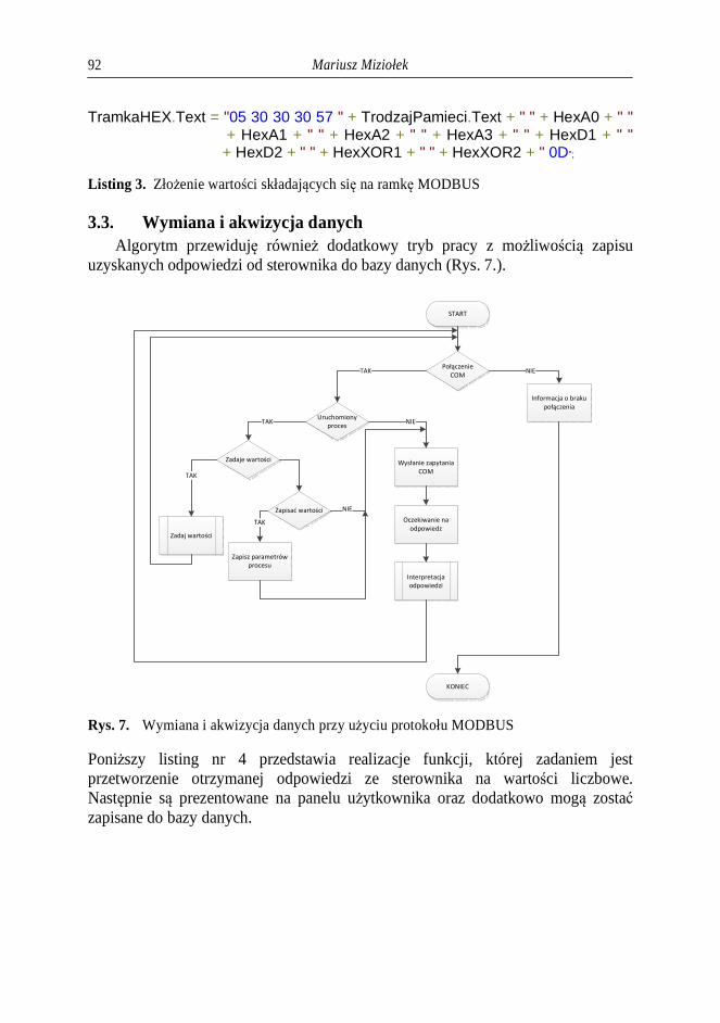
Mariusz Miziołek 92
TramkaHEX.Text = "05 30 30 30 57 " + TrodzajPamieci.Text + " " + HexA0 + " " + HexA1 + " " + HexA2 + " " + HexA3 + " " + HexD1 + " " + HexD2 + " " + HexXOR1 + " " + HexXOR2 + " 0D";
Listing 3. Złożenie wartości składających się na ramkę MODBUS
3.3. Wymiana i akwizycja danych Algorytm przewiduję również dodatkowy tryb pracy z możliwością zapisu
uzyskanych odpowiedzi od sterownika do bazy danych (Rys. 7.).
START
KONIEC
Połączenie
COM
Informacja o braku
połączenia
NIE
Wysłanie zapytania
COM
Oczekiwanie na
odpowiedz
Interpretacja
odpowiedzi
Uruchomiony
proces
TAK
NIE
Zadaje wartości
TAK
Zadaj wartości
TAK
Zapisać wartości
Zapisz parametrów
procesu
TAK
NIE
Rys. 7. Wymiana i akwizycja danych przy użyciu protokołu MODBUS
Poniższy listing nr 4 przedstawia realizacje funkcji, której zadaniem jest przetworzenie otrzymanej odpowiedzi ze sterownika na wartości liczbowe. Następnie są prezentowane na panelu użytkownika oraz dodatkowo mogą zostać zapisane do bazy danych.

Algorytm i implementacja protokołu komunikacyjnego MODBUS … 93
private void radTextBox2_TextChanged(object sender, EventArgs e) if (komorka > 0) proba++; try int dl = radTextBox2.Text.Length; bool znalazlemKoniec = false; try string kon = radTextBox2.Text.Substring(radTextBox2.Text.Length - 2, 2).ToString(); if (kon.Equals("0D")) znalazlemKoniec = true; catch if (znalazlemKoniec) if (pamiecM) int int1 = 0; int int2 = 0; int int3 = 0; int int4 = 0; string bezPoczatku = radTextBox2.Text.Remove(0, 8); string wartosc = bezPoczatku.Remove(bezPoczatku.Length - 6, 6); int i = 1; int j = 0; int x = 1; string[] hex = new string[komorka]; int v = 0; string str = wartosc; int b = (wartosc.Length / 8); int z = 0; int y = 0; for (int c = 0; c < b; c++) try v++; int1 = Convert.ToInt32(str.Substring(0, 8).Substring(0, 2), 16); int2 = Convert.ToInt32(str.Substring(0, 8).Substring(2, 2), 16); int3 = Convert.ToInt32(str.Substring(0, 8).Substring(4, 2), 16); int4 = Convert.ToInt32(str.Substring(0, 8).Substring(6, 2), 16); str = str.Remove(0, 8); v++; char char1 = (char)int1; char char2 = (char)int2; char char3 = (char)int3; char char4 = (char)int4; string wartoscHex1 = char3.ToString() + char4.ToString(); string wartoscHex2 = char1.ToString() + char2.ToString(); try string[] bit1 = rozszerzBityM(ToBinary(Convert.ToInt32(wartoscHex1, 16))); string[] bit = rozszerzBityM(ToBinary(Convert.ToInt32(wartoscHex2, 16))); tablicaM[adress] = bit[0]; adress++; tablicaM[adress] = bit[1]; adress++; tablicaM[adress] = bit[2]; adress++; tablicaM[adress] = bit[3]; adress++; tablicaM[adress] = bit[4]; adress++; tablicaM[adress] = bit[5]; adress++; tablicaM[adress] = bit[6]; adress++; tablicaM[adress] = bit[7]; adress = adress + 3; tablicaM[adress] = bit1[0]; adress++; tablicaM[adress] = bit1[1]; adress++;
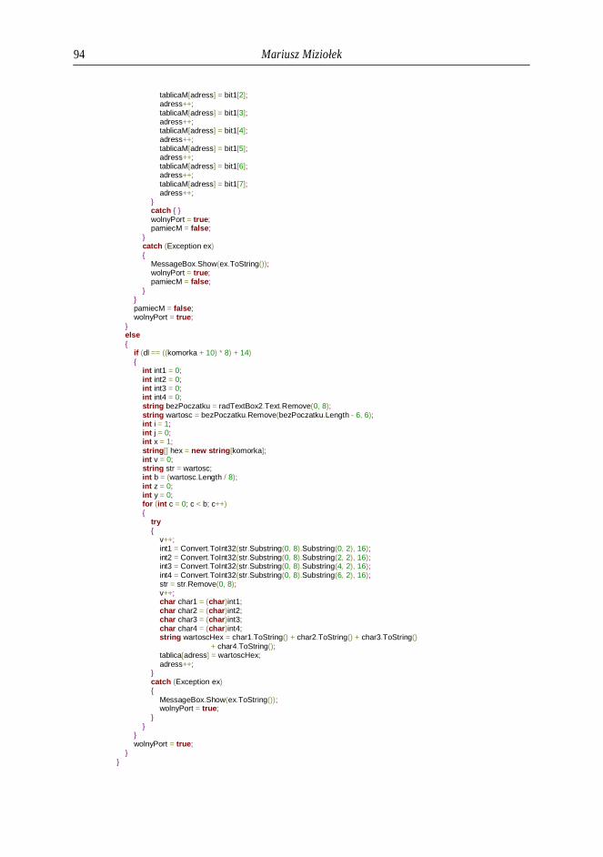
Mariusz Miziołek 94
tablicaM[adress] = bit1[2]; adress++; tablicaM[adress] = bit1[3]; adress++; tablicaM[adress] = bit1[4]; adress++; tablicaM[adress] = bit1[5]; adress++; tablicaM[adress] = bit1[6]; adress++; tablicaM[adress] = bit1[7]; adress++; catch wolnyPort = true; pamiecM = false; catch (Exception ex) MessageBox.Show(ex.ToString()); wolnyPort = true; pamiecM = false; pamiecM = false; wolnyPort = true; else if (dl == ((komorka + 10) * 8) + 14) int int1 = 0; int int2 = 0; int int3 = 0; int int4 = 0; string bezPoczatku = radTextBox2.Text.Remove(0, 8); string wartosc = bezPoczatku.Remove(bezPoczatku.Length - 6, 6); int i = 1; int j = 0; int x = 1; string[] hex = new string[komorka]; int v = 0; string str = wartosc; int b = (wartosc.Length / 8); int z = 0; int y = 0; for (int c = 0; c < b; c++) try v++; int1 = Convert.ToInt32(str.Substring(0, 8).Substring(0, 2), 16); int2 = Convert.ToInt32(str.Substring(0, 8).Substring(2, 2), 16); int3 = Convert.ToInt32(str.Substring(0, 8).Substring(4, 2), 16); int4 = Convert.ToInt32(str.Substring(0, 8).Substring(6, 2), 16); str = str.Remove(0, 8); v++; char char1 = (char)int1; char char2 = (char)int2; char char3 = (char)int3; char char4 = (char)int4; string wartoscHex = char1.ToString() + char2.ToString() + char3.ToString() + char4.ToString(); tablica[adress] = wartoscHex; adress++; catch (Exception ex) MessageBox.Show(ex.ToString()); wolnyPort = true; wolnyPort = true;

Algorytm i implementacja protokołu komunikacyjnego MODBUS … 95
catch (Exception ex) MessageBox.Show(ex.ToString()); wolnyPort = true;
Listing 4. Zaproponowana funkcja interpretująca odpowiedź sterownika.
Funkcja przetwarzająca odpowiedź sterownika przedstawiona na listingu 4 w wyniku swojego działania i przekształceń prowadzonych na odpowiedzi zwraca tablicę "tablica", w której indeks odpowiada adresowi zmiennej, a zawartość jest odczytaną wartością zmiennej zaprezentowaną w formie dziesiętnej.
4. Podsumowanie i możliwości rozwoju Opracowanie algorytmu do obsługi protokołu MODBAS RTU przy użyciu
języka programowania C# powstało w celu zaimplementowania tego rozwiązania w aplikacji do harmonogramowania procesu azotowania (Rys. 1), która powstała dla Instytutu Technologii Eksploatacji - PIB w Radomiu. Poprawność algorytmu została zweryfikowania poprzez przeprowadzenie procesu stabilizacji retorty oraz azotowania które trwały odpowiednio 24 godziny i 8 godzin. Algorytm można rozwijać poprzez optymalizacje czasu przetwarzania odpowiedź, dla zadania w którym został użyty nie zaistniała dodatkowa potrzeba zwiększenia prędkości działania.
Bibliografia 1. MODBUS [online], http://www.modbus.org/ 2. IDEC [online], http://www.idec.com/ 3. C# [online], https://msdn.microsoft.com/pl-pl/library/kx37x362.aspx 4. Kwaśniewski J.: Sterowniki PLC w praktyce inżynierskiej, ISBN
9788360233351 Wydawnictwo BTC, 2008. 5. Praca grupowa: Programowanie równoległe i asynchroniczne w C# 5.0, ISBN
9788324666980, Wydawnictwo Helion , 2013. 6. Templeman J., Vitter D.: Visual Studio .NET: .NET Framework. Czarna księga,
ISBN 8371977336, Wydawnictwo Helion , 2003 7. Daniluk A.: RS 232C - praktyczne programowanie. Od Pascala i C++ do Delphi
i Buildera. Wydanie III, ISBN 8324607781, Wydawnictwo Helion, 2007.

Mariusz Miziołek 96
Abstract The article concerns the construction and use of an algorithm for
communication via MODBUS RTU communication protocol used in IDEC PLCs. The main task of this algorithm is to build frames in MODBUS RTU standard transmission for their assistance requests to the controller and the interpretation of the replies sent by the driver. The practical part of the work brought to the development of C # code for developed algorithm and necessary validation activities for later use in other applications. Keywords: microcontroller, PLC, C#, Modbus communication protocol, industrial automation, IDEC
Streszczenie Artykuł dotyczy budowy oraz zastosowania algorytmu do komunikacji przez
protokół komunikacyjny MODBUS RTU wykorzystywany w sterownikach PLC firmy IDEC. Głównym zadaniem tego algorytmu jest budowanie ramek w standardzie MODBUS RTU przesyłanie za ich pomocą zapytania do sterownika oraz interpretacja odpowiedzi przesyłanych przez sterownik. Część praktyczna pracy sprowadziła się do opracowania kodu C# dla opracowanego algorytmu oraz wykonanie niezbędnych weryfikacji poprawności działania w celu późniejszego wykorzystania w inne aplikacji.

Walery Susłow, Michał Statkiewicz Wydział Elektroniki i Informatyki Jacek Kowalczyk Wydział Technologii i Edukacji Politechnika Koszalińska ul. J. J. Śniadeckich 2 75-453 Koszalin Marta Boińska, Janina Nowak Wydział Nauk Społecznych Uniwersytet Gdański ul. Jana Bażyńskiego 4 80-952 Gdańsk
Cechy osobowości studentów informatyki w kontekście gotowości zawodowej
Słowa kluczowe: programista, jakość oprogramowania, przygotowanie zawodowe, wczesne diagnozowanie, testy psychologiczne
1. Teoretyczne podstawy badań Artykuł przedstawia wyniki uzyskane w trakcie kontynuacji badań
prowadzonych od roku 2013 na Politechnice Koszalińskiej i na Uniwersytecie Gdańskim w ramach interdyscyplinarnego projektu InfoPsycho. Na pierwszym etapie badań zostało wykazane [1, 2], że studenci kierunku Informatyka, dobrze rokujący w pełnieniu roli projektanta oprogramowania, charakteryzują się wyższym poziomem takich cech osobowości jak neurotyczność i introwersja w porównaniu z kolegami i koleżankami, które nie wykazują tak wysokiego poziomu gotowości zawodowej. Celem niniejszego artykułu jest detaliczna analiza wybranych cech osobowości, będących korelatami neurotyczności. W badaniach doświadczalnych na grupie 93 osób w wieku około 23 lat sprawdzano, w jakim stopniu takie cechy jak samoskuteczność, wrażliwość empatyczna, kontrola emocjonalna, pośpiech, rywalizacja i poczucie stresu psychologicznego (patrz 1.2) mogą być czynnikami predykcyjnymi (charakteryzującymi przyszłych deweloperów oprogramowania). Formalnie rzecz ujmując, prezentowane badania są nastawione na rozwiązanie praktycznego problemu prognozowania wskaźnika syntetycznego "gotowość zawodowa studentów informatyki".

Walery Susłow, Michał Statkiewicz, Jacek Kowalczyk, Marta Boińska, Janina Nowak 98
W psychologii stosowanej gotowość zawodowa (profesjonalna gotowość, ang. professional readiness, ros. профессиональная готовность) jest terminem ujmującym predyspozycję jednostki do wykonania pracy zawodowej i do dalszego rozwoju zawodowego na podstawie doświadczeń i szkoleń. Ogólnie rzecz ujmując, gotowość do aktywności zawodowej jest uważana za aktualny stan osoby, który powoduje skuteczną działalność zawodową. Jednocześnie, gotowość zawodowa jest konsekwencją działalności zawodowej. Gotowość zawodowa określa nastawienie jednostki na sytuację zawodową i na wykonanie zadań zawodowych, jest ona uważana za warunek konieczny do działania celowego, jego regulacji, stabilności i efektywności [3].
Koncepcja profesjonalnej gotowości jest postrzegana jako kategoria teorii aktywności [4]. Uważa się, że struktura organizacyjna profesjonalnej gotowości w powszechnych przejawach jest inwariantem w konkretnym rodzaju działalności zawodowej. Personalna gotowość zawodowa jest rozwijana przez poszczególne doświadczenia zawodowe. Można przyjąć, że w okresie studiów studenci tworzą własną podstawę do przyszłego zatrudnienia, do aktywności zawodowej, czyli kształtują stan gotowości zawodowej. Zakłada się, że model gotowości zawodowej pozostaje niezmienny w ostatnich dziesięcioleciach, typowy dla pełnionych funkcji w danym zawodzie, ale stan faktyczny gotowości zawodowej jest zmienny w indywidualnych przejawach.
Gotowość zawodowa jest syntetycznym wskaźnikiem, którego struktury nie udało się jeszcze sformalizować, a więc nie jest ona bezpośrednio dostępna do dekompozycji. Jednak strukturę gotowości zawodowej można modelować teoretycznie na podstawie podejścia systemowego. W praktyce gotowość zawodowa jest badana (testowana) i jako stan świadomości, psychiki, i jako stan systemów funkcjonalnych jednostki w sytuacji działania w sposób odpowiedzialny oraz w sytuacji przygotowania się do takich działań (nauka, szkolenia, ćwiczenia itd.). W ramach niniejszego artykułu gotowość zawodowa została zoperacjonalizowana w formie integralnego wskaźnika, wyrażającego poziom nabytej wiedzy i umiejętności zawodowych z zakresu programowania komputerów, projektowania aplikacji komputerowych i pracy zespołowej. Ten wskaźnik określa skuteczność (sprawność, produktywność, wydajność) studenta w kontekście jego indywidualnej dydaktycznej aktywności deweloperskiej (analitycznej, projektowej, implementacyjnej i testowej). Szczegóły skali oraz procedury oceniania gotowości zawodowej zostały przedstawione w rozdziale 2 niniejszego artykułu.
1.1. Dobór badanych zmiennych psychologicznych Informatyka pozostaje jednym z najczęściej wybieranych kierunków studiów
[5], a uczelnie techniczne, prowadzące studia na kierunkach informatycznych, stoją przed wyzwaniem dynamicznego dopasowywania oferty edukacyjnej z zakresu IT do zapotrzebowań dynamicznie rozwijającego się rynku technologii i usług

Cechy osobowości studentów informatyki w kontekście gotowości zawodowej 99
informatycznych. Testy psychologiczne do wczesnego diagnozowania efektywnych deweloperów oprogramowania powinny stanowić jedną z technik wspomagających dostosowanie oferty edukacyjnej wyższych uczelni do potrzeb rynku pracy.
Nauka programowania komputerów jest procesem trudnym i złożonym, oraz w znacznym stopniu doświadczeniem indywidualnym dla każdego studenta. Z pewnością wiadomo, że pierwsze lata studiów informatycznych charakteryzują się wysokim odsetkiem osób rezygnujących z kontynuowania nauki. Stąd istotnym jest poznanie mechanizmów wpływających na decyzje o kontynuowaniu studiów informatycznych oraz na rozpoznanie elementów decydujących o osiągnięciach studentów kierunku Informatyka. Domyślnie można spodziewać się, że takie organizacyjne uwarunkowania jak osobiste doświadczenie studentów w tworzeniu oprogramowania i style uczenia się będą kluczowymi składnikami sukcesu w opanowaniu zawodu.
Niewiele jest wyników badań nad psychologicznymi uwarunkowaniami, wpływającymi na przebieg studiów dla kierunków informatycznych. Dotychczasowe badania niniejszego zespołu autorskiego wykazały, że psychologiczne uwarunkowania mogą uczestniczyć w kształtowaniu sukcesów zawodowych młodego informatyka. Badania ukazały, że osiągnięcie przez studentów dobrych nawyków deweloperskich koreluje z konkretnymi wymiarami osobowości w pięcioczynnikowym modelu osobowości Costy i McCrae [6]. Stwierdzono dodatnią korelację, między jakością projektowanego przez nich oprogramowania a poziomem neurotyzmu oraz introwersji wykonawców. Studenci z najwyższym stopniem efektywności w zakresie projektowania oprogramowania okazali się bardziej neurotyczni od studentów z gorszymi wynikami. Zaobserwowano również różnice wewnątrzgrupowe dla ekstrawersji. Stwierdzono, że studenci dostarczający wysokojakościową dokumentację projektową i wyróżniający się komunikatywnością w trakcie prac projektowych byli mniej ekstrawertyczni niż studenci o gorszych wynikach zawodowych. Ponad to studenci z najwyższym stopniem efektywności w zakresie projektowania oprogramowania okazali się mniej stabilni emocjonalnie [2].
Po zakończeniu badań pilotażowych zespół badawczy InfoPsycho zdecydował przeprowadzić detaliczne badania wybranych zmiennych psychologicznych w kontekście diagnozowania predyspozycji zawodowych studentów-informatyków. Na podstawie uzyskanych danych pilotażowych i kwerendy literatury, zespół zdecydował w pierwszej kolejności zbadać doświadczalnie zmienne psychologiczne, będące korelatami neurotyczności, a mianowicie: samoskuteczność, empatię, kontrolę emocjonalną, pośpiech i rywalizację oraz poziom stresu. Według założeń zespołu, różnice indywidualne w zakresie tych zmiennych mogłyby wpływać na proces projektowania (programowania) i być kluczem do zrozumienia procesu skutecznego nauczania i uczenia się zawodu informatyka.

Walery Susłow, Michał Statkiewicz, Jacek Kowalczyk, Marta Boińska, Janina Nowak 100
Nowoczesna psychologia stosowana dysponuje rozmaitymi narzędziami do testowania cech osobowości i pomiaru wybranych zmiennych. W dalszej części niniejszego rozdziału zostaną przedstawione modele konceptualne, które posłużyły zespołowi teoretyczną podstawą do planowania badań i interpretacji ich wyników.
1.2. Modele psychologiczne Konstrukt samoskuteczności Bandury. Konstrukt samoskuteczności jest
dobrze udokumentowany w literaturze, powstał on w kontekście teorii społecznego uczenia się [7]. Osoba, która posiada wysoki poziom samoskuteczności, opisywana jest jako osoba aktywna, posiadająca zdolności do dokonywania wyborów i posiadająca potencjał by rozwijać się nieustannie, niezależnie od czynników zewnętrznych. Badania wskazują, że posiadanie przekonania o własnej skuteczności, może wpływać na poziom motywacji i bezpośrednie podejmowanie działań. Jest to istotna konkluzja, gdyż wskazuje ona na to, że podnoszenie samoświadomości własnej skuteczności może być kluczem do wysokiej wydajności w nauce. Ponadto, coraz więcej badaczy popiera stosowanie modelu własnej skuteczności w pomiarze efektywności programów edukacyjnych [8]. Za autorem koncepcji A. Bandurą w niniejszym badaniu przyjęte zostało, że samoskuteczność to przekonanie o czyichś zdolnościach do organizowania i wykonywania działań niezbędnych do produkcji osiągnięć [9].
Inteligencja emocjonalna. W gospodarce poprzedniego stulecia głównie koncentrowano się na testowaniu i podnoszeniu takich zdolności pracowników jak ogólna inteligencja, skuteczność czy motywacja. Ostatnio możemy zaobserwować, że następuje pogłębienie refleksji nad zdrowym, a zatem i efektywnym budowaniem środowiska pracy. Środowisko biznesu IT nie różni się pod tym względem od innych gałęzi gospodarki. Ze względu na zespołową specyfikę pracy działy kadr (ang. Human Resources) w IT poszukują pracowników nie tylko inteligentnych w rozumieniu powszechnym, ale też tych, którzy będą potrafili dzielić się wiedzą, umiejętnie współpracować w grupie, utrzymywać dobre relacje z współpracowni-kami niezależnie od języka czy kultury, w której się wychowali. Czyli poszukiwani są informatycy (programiści) uzdolnieni emocjonalnie. Tą tendencję możemy obserwować już od 1999 roku, gdyż dokładnie w tym roku Daniel Goleman przeprowadził międzynarodowe badania na milionach pracowników w 121 organizacjach i przedsiębiorstwach, które wykazały, że ponad 2/3 kompetencji szczególnie pożądanych by skutecznie wykonywać pracę to kompetencje emocjonalne. Niezależnie od rodzaju przedsiębiorstwa czy organizacji to właśnie zdolności emocjonalne przewyższały wiedzę fachową oraz inteligencję [10]. Wnioski z tego badania mają ścisły związek z empatią, gdyż Daniel Goleman wskazywał na empatię jako jeden z pięciu czynników odgrywających kluczową role w inteligencji emocjonalnej [11]. Daniel Goleman i Richard Boyatzis [11] wykazali w swoich badaniach, że programiści, którzy posiadali wysoki poziom inteligencji

Cechy osobowości studentów informatyki w kontekście gotowości zawodowej 101
emocjonalnej, rozwijali efektywne oprogramowanie trzy razy szybciej od innych programistów. Inne badania wykazały, że interwencje z poziomu inteligencji emocjonalnej miały pozytywny wpływ tak na proces tworzenia programowania jak i na ostateczny kształt produktu [12].
Kontrola emocjonalna. Z pojęciem empatii i inteligencji emocjonalnej ściśle wiążę się kontrola emocjonalna, która również jest rozpatrywana jako element kompetencji emocjonalnych. Dojrzała kontrola emocjonalna charakteryzuje się plastycznością, możliwością wyboru sposobu ekspresji swoich emocji i adaptacyjnością [13]. Osoba z rozwiniętą kontrolą emocjonalną potrafi w niektórych sytuacjach hamować swoje emocje, a w innych − swobodnie je ujawniać. Zdaniem Brzezińskiego kontrola emocjonalna to „mechanizm psychologiczny określający zdolność jednostki do umiejętnego wyrażania swoich stanów emocjonalnych zależnie od kontekstu sytuacyjnego” [14]. Zgodnie z tym podejściem kontrola emocjonalna została zoperacjonalizowana w niniejszej pracy. Zaś empatia w niniejszym badaniu została ujęta za Uchnast, jako postawa charakterologiczna pełna autentyczności, otwartości, szacunku wobec innych ludzi oraz dążenia do zrozumienia cudzych doświadczeń w całej ich złożoności, a także jako wrażliwość na przeżycia innych ludzi oraz chęć zrozumienia ich preferencji i poglądów [15].
Stres a teoria Lazarusa. W sektorze IT powszechne jest występowanie wysokiego odczuwania stresu wśród pracowników, wynika to ze specyfiki pracy skoncentrowanej na ściśle zdefiniowanych celach w krótkich okresach oraz z przeciążenia zadaniami [16]. Wiedza ta uzmysławia nam, na jakie ryzyko narażeni są potencjalni programiści. Jedno z badań prowadzonych nad stresem wśród pracowników IT ukazało, że ponad 51% z nich jest stale zestresowanych, co zwiększa dziesięciokrotnie ryzyko wystąpienia depresji w tej grupie zawodowej [17]. Ważnym w obliczu tych wyników jest by rozpoznać jak przyszli programiści radzą sobie ze stresem. Należy pamiętać, że studiowanie nie może być zredukowane jedynie do zdobywania wiedzy, jest ono również okresem zmian psychologicznych, socjologicznych i kulturalnych. Studenci stają przed kolejnymi zadaniami rozwojowymi, takimi jak podejmowanie niezależnych decyzji, kształtowanie sposobów radzenia sobie ze stresem czy kształtowanie nowych schematów uczenia się. Ten proces nie jest taki sam dla wszystkich studentów, niektórzy adaptują się do zmian łatwo i szybko, inni zaś zmagają się z tymi zmianami, a w konsekwencji doświadczają stresu [18]. Na potrzeby niniejszego badania definicja stresu została zaczerpnięta z teorii Lazarusa, określającej relację między osobą a otoczeniem. W ramach tej teorii otoczenie jest oceniane przez osobę jako obciążające lub przekraczające jej zasoby i zagrażające jej dobrostanowi [19].

Walery Susłow, Michał Statkiewicz, Jacek Kowalczyk, Marta Boińska, Janina Nowak 102
1.3. Cele badania i hipotezy Cele niniejszego badania zostały sformułowane w sposób następujący: określić
relacje samoskuteczności, odczuwanego stresu, poziomu empatii i kontroli emocjonalnej studentów-informatyków z poziomem ich gotowości zawodowej.
Oto hipotezy poddane weryfikacji w ramach postawionego celu: H1: Studenci o wyższej gotowości zawodowej będą charakteryzować się
wyższym poziomem samoskuteczności. H2: Studenci o wyższej gotowości zawodowej będą posiadali wyższy poziom
wrażliwości empatycznej oraz kontroli emocjonalnej. H3: Studenci o wyższej gotowości zawodowej będą wykazywać niższe wyniki
w skali pośpiechu i rywalizacji. H4: Studenci o wyższej gotowości zawodowej będą wykazywać niższy poziom
odczuwanego stresu.
1.4. Koncepcja prognozowania gotowości zawodowej studentów Do koordynacji wieloczynnikowych badań zespół badawczy opracował wstępny
model teoretyczny skuteczności zawodowej projektanta oprogramowania. Model ten będzie miał postać wielomianową, w której współczynniki wyznaczone będą na podstawie korelacji między badanymi cechami psychicznymi a osiągnięciami naukowymi i zawodowymi. Ogólna postać modelu jest następująca:
= (, , , , ), (1) gdzie:
– skuteczność zawodowa. Jest to zmienna prognozowana, funkcja celu. W kontekście obecnej publikacji jest to raczej skuteczność w nauce zawodu, oceniana na podstawie osiągnięć studentów, rejestrowanych w postaci średniej z ocen cząstkowych z projektów wykonywanych według planu semestralnego.
= Udział_w_projektach, Popularność_produktu, Jakość_produktu (2)
, – cechy psychiczne (cechy osobowości). Jest to wektor zmiennych opisujących członków badanej grupy, które mierzone są za pomocą testów psychologicznych o wysokiej trafności.
=Pi ęcioczynnikowy Model Osobowości PMO, Samoskuteczność, Stresoodporność, Empatia, Inteligencja, Kontrola_emocji (3)
– kondycja ogólna projektanta, mająca wpływ na jego skuteczność praktycznie w każdym działaniu. Niestety, jest to cecha zmienna w czasie oraz trudna do zmierzenia.

Cechy osobowości studentów informatyki w kontekście gotowości zawodowej 103
– wiedza zawodowa projektanta. Jest ona łatwo mierzalna na poziomie studenckim, kryteria pomiaru zostały opisane w [20-21]. W przypadku specjalisty po studiach może ona być opisywana poprzez zbiór certyfikatów, które można uznać za znormalizowane wskaźniki wiedzy zawodowej.
= Oceny, Aktywność, Komunikacja, Certyfikaty (4) – otoczenie projektanta (w tym ewentualny zespół projektowy), podobnie jak
ten składnik modelu może być kłopotliwy w pomiarze. – praca wykonana, czyli ciąg działań zawodowych oraz ich mierzalnych
rezultatów, które projektant osiągnął. W praktyce pełne dane mogą być trudne do uzyskania ze względu na poufność prac projektanckich, jednocześnie będąc łatwymi w kwantyfikacji dzięki istniejącym metodom wymiarowania projektów informatycznych.
Pozyskanie danych opisujących wszystkie składniki modelu wymaga kilku etapów badań, stąd obecnie model nie może być kompletny. Należy jeszcze zauważyć, że zastosowane na danym etapie testy psychologiczne obejmują szerokie spektrum cech psychicznych, zaś zmierzone wartości tych cech odzwierciedlają również wpływ szeregu czynników na projektantów. Stąd można wnioskować, że składniki modelu takie jak (kondycja ogólna) oraz O (otoczenie) można wyeliminować z modelu jako redundantne w stosunku do , (cech psychicznych), gdy te ostatnie będą obejmowały wpływy kondycji ogólnej i otoczenia na projektanta. Stąd ostateczna uproszczona postać modelu może być następująca:
= (, , ) (5)
2. Metodyka testowania
2.1. Charakterystyka badanych grup studenckich Grupę badaną stanowili studenci Wydziału Elektroniki i Informatyki
Politechniki Koszalińskiej, studiujący IV semestr kierunku Informatyka. Grupa składała się z 93 osób, wśród których 90% stanowili mężczyźni i 10% − kobiety. Średnia wieku osób badanych wynosiła 23 lat przy odchyleniu standardowym SD = 4.32.
Na podstawie wskaźników opisujących postępy w nauce grupa została podzielona na trzy podgrupy, składające się ze studentów wykazujących wysokie (bardzo dobre), przeciętne (dobre) oraz niskie (dostateczne) przygotowanie zawodowe.

Walery Susłow, Michał Statkiewicz, Jacek Kowalczyk, Marta Boińska, Janina Nowak 104
2.2. Pierwszy zestaw testów 1. Test psychologiczny GSES (Skala Uogólnionej Własnej Skuteczności Ralfa
Schwarzera, Michaela Jarusalem i Zygfryda Juczyńskiego, 2001) [22] – narzędzie mierzy siłę przekonania osoby, że potrafi ona wykonać konkretne działanie lub też zrealizować wyznaczone cele.
Kwestionariusz GSES składa się z 10 stwierdzeń, do których badany ustosunkowuje się na 4-stopniowej skali odpowiedzi: „Tak”, „Raczej tak”, „Raczej nie” i „Nie”.
Kwestionariusz cechuje się wysoką rzetelnością i trafnością [22]. 2. Test psychologiczny SWE (Skala Wrażliwości Empatycznej Marii
Kaźmierczak, Mieczysława Plopy i Sylwiusza Retowskiego, 2007) [23] – narzędzie mierzy poziom empatii (reagowania na doświadczenie innych osób) w trzech wymiarach, którym odpowiadają trzy podskale kwestionariusza:
Podskala empatycznej troski (ET) – opisuje uczucia skierowane na drugiego człowieka: współczucie i współodczuwanie w stosunku do osób dotkniętych nieszczęściem. Im wyższy wynik badany osiąga na tej skali, tym wyższy jego poziom empatycznej troski.
Podskala Osobistej Przykrości (OP) – opisuje uczucia ukierunkowane na siebie: poziom przeżywania strachu, niepokoju, przykrości w reakcji na silne uczucia negatywne (cierpienie) innych osób. Im wyższy wynik badany osiąga na tej skali, tym wyższy jego poziom osobistej przykrości.
Podskala przyjmowania perspektywy (PP) – mierzy umiejętność i skłonność do przyjmowania punktu widzenia drugiej osoby w sytuacjach codziennych. Im wyższy wynik badany osiąga na tej skali, tym wyższy jego poziom przyjmowania perspektywy.
Kwestionariusz SWE składa się z 28 stwierdzeń, do których badani ustosunkowują się na 5-stopniowej skali odpowiedzi: od „całkowicie się nie zgadzam” do „zdecydowanie się zgadzam". Wynik ogólny kwestionariusza oblicza się poprzez zsumowanie wyników z trzech podskal: ET, OP i PP.
Narzędzie cechuje się wysoką rzetelnością i trafnością [23]. 3. Test psychologiczny KKE (Kwestionariusz Kontroli Emocjonalnej Jerzego
Brzezińskiego, 1972) [24] – narzędzie mierzy stopień samokontroli emocjonalnej osoby na różnych etapach procesu emocjonalnego: 1) spostrzegania i interpretacji sytuacji emotogennej; 2) reakcji fizjologicznej i procesu motywacyjnego oraz 3) działania pod wpływem emocji. Test składa się z czterech podskal:
Podskala kontroli ekspresji (Ke) – wskazuje na stopień, w jakim osoba jest w stanie kontrolować zewnętrzne przejawy doświadczanych emocji, jak np. mimikę twarzy, ton głosu, ruchy całego ciała, śmiech, płacz. Wysoki wynik oznacza nadmierną kontrolę ekspresji emocji, wynik niski – jej słabą kontrolę.

Cechy osobowości studentów informatyki w kontekście gotowości zawodowej 105
Podskala motywacji emocjonalno-racjonalnej (Mer) – określa typ sterowania własnym zachowaniem. Wysoki wynik w tej skali wskazuje, że osoba ma skłonność do zachowywania się w sposób kontrolowany i przemyślany, niski wynik oznacza skłonność do zachowań impulsywnych.
Podskala odporności emocjonalnej (Oe) – mierzy stopień, w jakim osoba jest w stanie kontrolować rozwijający się w niej proces emocjonalny i nie dezorganizować się pod jego wpływem. Osoby osiągające wysokie wyniki na tej skali są odporne na działanie emocji oraz nadmiernie kontrolują swoje zachowanie, osoby osiągające niski wynik – poddają się działaniu emocji i nie kontrolują własnego zachowania.
Podskala kontroli sytuacji (Ks) – informuje o tym, czy osoba łatwo wchodzi w sytuacje wzbudzające emocje czy też raczej ich unika. Wysoki wynik na tej skali oznacza dążenie do nadmiernej kontroli sytuacji, przejawiające się głównie lękiem; niski wynik świadczy o tym, że osoba zbyt łatwo wchodzi w sytuacje emocjonalne bez uwzględniania wynikających z tego konsekwencji.
Kwestionariusz KKE składa się z 45 pozycji. Badanego prosi się, by się do nich ustosunkował na 4-stopniowej skali odpowiedzi; zawsze, często, rzadko, nigdy. Wskaźnik ogólny stanowi suma wyników surowych w czterech podskalach: Ke, Mer, Oe i Ks.
Test KKE cechuje się zadowalającą rzetelnością i trafnością [24].
2.3. Drugi zestaw testów 4. Test psychologiczny Typ-A (Skala Typu A-Framingham Zygfryda
Juczyńskiego, 2001) zawiera 10 stwierdzeń, z których pięć pierwszych dotyczy cech i właściwości typowych dla jednostki, kolejne cztery – odczuć pod koniec przeciętnego dnia, wreszcie ostatnie – presji czasu. W polskiej wersji skala obejmuje dwa czynniki charakteryzujące osobowość typu A (wzór zachowania A) – pośpiech i rywalizację. Wyniki oblicza się poprzez zsumowanie odpowiedzi i podzielenie ich przez liczbę pytań. Pytania zawarte w drugiej części Skali Typu A, dotyczą pracy zawodowej (czy jednostka wykonuje swoje obowiązki działając w pośpiechu, czy rywalizuje z innymi) [22]. Kwestionariusz cechuje się wysoką rzetelnością i trafnością.
5. Test psychologiczny KPS (Kwestionariusz Poczucia Stresu Mieczysława Plopy i Ryszarda Makarowskiego, 2010) przeznaczony jest do pomiaru struktury doznań stresowych, składa się z 27 stwierdzeń. Pozwala na obliczenie wyniku ogólnego informującego o uogólnionym poziomie stresu, a także trzech wyników odnoszących się do następujących wymiarów: napięcie emocjonalne, stres zewnętrzny oraz stres intrapsychiczny. Napięcie emocjonalne wynika z poczucia niepokoju, nadmiernej nerwowości. Występuje w różnych codziennych sytuacjach, gdy pojawiają się trudności w odprężaniu się. Związane jest z brakiem energii do

Walery Susłow, Michał Statkiewicz, Jacek Kowalczyk, Marta Boińska, Janina Nowak 106
działania, poczuciem zmęczenia bez wyraźnej przyczyny, jak i z tendencją do rezygnacji z podejmowania różnych zadań, realizacji planów. Stres zewnętrzny pojawia się, gdy jest się niesprawiedliwie ocenianym przez inne osoby w różnych kontekstach społecznych, gdy narasta poczucie bezradności, wyczerpania w obronie swojego punktu widzenia (swoich racji). Stres intrapsychiczny jest związany z nieumiejętnością radzenia sobie z przeżyciami wewnętrznymi. System psychiczny pełen napięcia i konfliktów nie potrzebuje zewnętrznych nacisków do odczuwania stresu. Ten rodzaj stresu występuje, gdy ma się problemy ze sobą, ciągłymi doświadczeniami z przeszłości dającymi objawy osamotnienia i niepokoju. Kwestionariusz zawiera też skalę Kłamstwa. Skala ta zawiera siedem twierdzeń, do których osoba badana ustosunkowuje się w pięciostopniowej skali Likerta: od prawda do nieprawda. Wyniki oblicza się poprzez zsumowanie punktowanych (od 1 do 5) odpowiedzi. Kwestionariusz cechuje się wysoką rzetelnością i trafnością dla wszystkich podskal [25].
3. Prezentacja wyników analizy statystycznej W celu porównania trzech podgrup studentów: wysoko rokujących,
przeciętnych oraz nisko rokujących projektantów oprogramowania pod względem wybranych zmiennych psychologicznych zastosowano dwa rodzaje testów statystycznych [26]: analizę wariancji ANOVA dla grup niezależnych, gdy założenie o jednorodności wariancji zostało spełnione oraz test Welcha w przypadku niespełnienia tego warunku. Homogeniczność wariancji badanych grup sprawdzono przy użyciu testu Levene’a.
Dla badań statystycznych ustalono poziom alfa < 0.1. Analizę statystyczną przeprowadzono przy użyciu programu IBM SPSS Statistics 22.
Dwie fazy badania psychologicznego, polegające na wypełnieniu przez osoby badane dwóch różnych zestawów testów w odstępie dwóch tygodni, znalazły odzwierciedlenie w sposobie prezentacji wyników. Tabela 1 zawiera wyniki testów z zestawu 1, a tabela 2 − z zestawu 2.
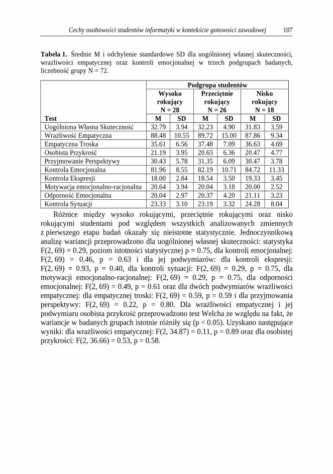
Cechy osobowości studentów informatyki w kontekście gotowości zawodowej 107
Tabela 1. Średnie M i odchylenie standardowe SD dla uogólnionej własnej skuteczności, wrażliwości empatycznej oraz kontroli emocjonalnej w trzech podgrupach badanych, liczebność grupy N = 72.
Test
Podgrupa studentów Wysoko rokuj ący N = 28
Przeciętnie rokuj ący N = 26
Nisko rokuj ący N = 18
M SD M SD M SD Uogólniona Własna Skuteczność 32.79 3.94 32.23 4.90 31.83 3.59 Wrażliwość Empatyczna 88.48 10.55 89.72 15.00 87.86 9.34 Empatyczna Troska 35.61 6.56 37.48 7.09 36.63 4.69 Osobista Przykrość 21.19 3.95 20.65 6.36 20.47 4.77 Przyjmowanie Perspektywy 30.43 5.78 31.35 6.09 30.47 3.78 Kontrola Emocjonalna 81.96 8.55 82.19 10.71 84.72 11.33 Kontrola Ekspresji 18.00 2.84 18.54 3.50 19.33 3.45 Motywacja emocjonalno-racjonalna 20.64 3.94 20.04 3.18 20.00 2.52 Odporność Emocjonalna 20.04 2.97 20.37 4.20 21.11 3.23 Kontrola Sytuacji 23.33 3.10 23.19 3.32 24.28 8.04
Różnice między wysoko rokującymi, przeciętnie rokującymi oraz nisko rokującymi studentami pod względem wszystkich analizowanych zmiennych z pierwszego etapu badań okazały się nieistotne statystycznie. Jednoczynnikową analizę wariancji przeprowadzono dla uogólnionej własnej skuteczności: statystyka F(2, 69) = 0.29, poziom istotności statystycznej p = 0.75, dla kontroli emocjonalnej: F(2, 69) = 0.46, p = 0.63 i dla jej podwymiarów: dla kontroli ekspresji: F(2, 69) = 0.93, p = 0.40, dla kontroli sytuacji: F(2, 69) = 0.29, p = 0.75, dla motywacji emocjonalno-racjonalnej: F(2, 69) = 0.29, p = 0.75, dla odporności emocjonalnej: F(2, 69) = 0.49, p = 0.61 oraz dla dwóch podwymiarów wrażliwości empatycznej: dla empatycznej troski: F(2, 69) = 0.59, p = 0.59 i dla przyjmowania perspektywy: F(2, 69) = 0.22, p = 0.80. Dla wrażliwości empatycznej i jej podwymiaru osobista przykrość przeprowadzono test Welcha ze względu na fakt, że wariancje w badanych grupach istotnie różniły się (p < 0.05). Uzyskano następujące wyniki: dla wrażliwości empatycznej: F(2, 34.87) = 0.11, p = 0.89 oraz dla osobistej przykrości: F(2, 36.66) = 0.53, p = 0.58.
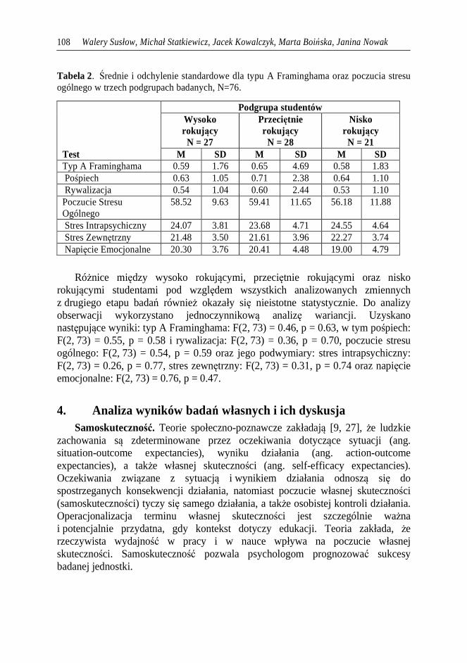
Walery Susłow, Michał Statkiewicz, Jacek Kowalczyk, Marta Boińska, Janina Nowak 108
Tabela 2. Średnie i odchylenie standardowe dla typu A Framinghama oraz poczucia stresu ogólnego w trzech podgrupach badanych, N=76.
Test
Podgrupa studentów Wysoko rokuj ący N = 27
Przeciętnie rokuj ący N = 28
Nisko rokuj ący N = 21
M SD M SD M SD Typ A Framinghama 0.59 1.76 0.65 4.69 0.58 1.83 Pośpiech 0.63 1.05 0.71 2.38 0.64 1.10 Rywalizacja 0.54 1.04 0.60 2.44 0.53 1.10 Poczucie Stresu Ogólnego
58.52 9.63 59.41 11.65 56.18 11.88
Stres Intrapsychiczny 24.07 3.81 23.68 4.71 24.55 4.64 Stres Zewnętrzny 21.48 3.50 21.61 3.96 22.27 3.74 Napięcie Emocjonalne 20.30 3.76 20.41 4.48 19.00 4.79
Różnice między wysoko rokującymi, przeciętnie rokującymi oraz nisko rokującymi studentami pod względem wszystkich analizowanych zmiennych z drugiego etapu badań również okazały się nieistotne statystycznie. Do analizy obserwacji wykorzystano jednoczynnikową analizę wariancji. Uzyskano następujące wyniki: typ A Framinghama: F(2, 73) = 0.46, p = 0.63, w tym pośpiech: F(2, 73) = 0.55, p = 0.58 i rywalizacja: F(2, 73) = 0.36, p = 0.70, poczucie stresu ogólnego: F(2, 73) = 0.54, p = 0.59 oraz jego podwymiary: stres intrapsychiczny: F(2, 73) = 0.26, p = 0.77, stres zewnętrzny: F(2, 73) = 0.31, p = 0.74 oraz napięcie emocjonalne: F(2, 73) = 0.76, p = 0.47.
4. Analiza wyników badań własnych i ich dyskusja Samoskuteczność. Teorie społeczno-poznawcze zakładają [9, 27], że ludzkie
zachowania są zdeterminowane przez oczekiwania dotyczące sytuacji (ang. situation-outcome expectancies), wyniku działania (ang. action-outcome expectancies), a także własnej skuteczności (ang. self-efficacy expectancies). Oczekiwania związane z sytuacją i wynikiem działania odnoszą się do spostrzeganych konsekwencji działania, natomiast poczucie własnej skuteczności (samoskuteczności) tyczy się samego działania, a także osobistej kontroli działania. Operacjonalizacja terminu własnej skuteczności jest szczególnie ważna i potencjalnie przydatna, gdy kontekst dotyczy edukacji. Teoria zakłada, że rzeczywista wydajność w pracy i w nauce wpływa na poczucie własnej skuteczności. Samoskuteczność pozwala psychologom prognozować sukcesy badanej jednostki.

Cechy osobowości studentów informatyki w kontekście gotowości zawodowej 109
W badaniu studentów-informatyków zaobserwowano najwyższy poziom własnej skuteczności w grupie wysoko rokujących projektantów oprogramowania, niższy − w grupie średnio rokujących, a najniższy − w grupie nisko rokujących. Jednak nie są to różnice istotne statystycznie, dlatego też hipoteza nr 1 została odrzucona. Ważne jest to, że wszyscy badani wykazali się wysoką samoskutecznością – osiągnęli 8. sten w skali GSES. Przyjmuje się, że studenci z wysokim poczuciem własnej skuteczności działania są bardziej skłonni do podejmowania trudnych zadań i do znacznie większego wysiłku w procesie wykonania tych zadań w obliczu pojawiających się trudności, niż studenci z niskim poczuciem własnej skuteczności [8].
Porównując studentów z identycznymi umiejętnościami poznawczymi, można zauważyć, że studenci z wyższymi wskaźnikami samoskuteczności są bardziej konsekwentni w realizacji celów. Natomiast studenci osiągający niższe wskaźniki samoskuteczności mają tendencje do wyolbrzymiania problemów, na problemy reagują stresem, depresją, co może sprawiać, że powierzone im zadania stają się dla nich nierozwiązywalne [28]. Bandura był zdania, że poczucie własnej skuteczności rozwija się stopniowo wraz z osiągnięciem umiejętności i doświadczenia. Badania wykazują, że w obszarze programowania poziom samoskuteczności jest istotnie uwarunkowany umiejętnościami i doświadczeniem programistów [8].
Wrażliwość empatyczna. W teorii zakłada się, że empatia odgrywa centralną rolę w interakcjach społecznych, zarówno w relacjach nieformalnych, jak i zawodowych [29]. Zdolność do przejawu empatii stała się szczególnie istotna w zglobalizowanym świecie, charakteryzującym się intensywną komunikacją międzykulturową. Taka zdolność powinna być szczególnie cenna w sytuacji współpracy interdyscyplinarnej, zwłaszcza wtedy, gdy inżynierowie w swojej pracy zawodowej wchodzą w interakcje z różnymi grupami zawodowymi, docierają do różnych grup odbiorców (użytkowników oprogramowania). Zdaniem autora koncepcji inteligencji emocjonalnej, Davida Golemana [30], edukacja inżynierów nie koncentruje się na rozwoju takich cech osobowości jak empatia, co szczególnie widać wśród inżynierów zajmujących stanowiska kierownicze. Inżynierowie specjalizujący się w programowaniu, oprócz kompetencji kluczowych w ramach danej dziedziny wiedzy, powinni nabywać umiejętności w obszarze kompetencji miękkich, a także wykazywać się empatią. Mogłoby to skutkować zwiększoną skutecznością pracy zespołowej oraz polepszeniem komunikacji zespołu IT z interesariuszami projektu. Wbrew oczekiwaniom, wyniki naszych badań nie pokazują, że wrażliwość empatyczna różnicuje badane podgrupy studentów. Wszyscy badani uzyskali przeciętne (w skali SWE) wyniki w obszarze empatii.
Kontrola emocjonalna. Stany emocjonalne są jednymi z głównych źródeł własnej skuteczności jednostki. Kontrola emocji − to proces, za pomocą którego jednostka może wpływać na to jakie przeżywa emocje, kiedy się one zaostrzają, jak je ocenia, jak je wyraża. Ludzie różnią się sposobem interpretacji swoich stanów

Walery Susłow, Michał Statkiewicz, Jacek Kowalczyk, Marta Boińska, Janina Nowak 110
emocjonalnych i te stany emocjonalne wpływają na ich ocenę własnych kompetencji. W kontekście pracy zawodowej informatyków, utrzymywanie własnych emocji w ryzach jest szczególnie ważne podczas kontaktów z klientami [31]. Szczególnie w rozmowach z przyszłymi klientami, którzy będą oczekiwać, że dostawcy oprogramowania zapewnią im jak najwięcej korzyści przy minimalnych kosztach.
Zdolność kontroli emocjonalnej jest również bardzo ważna, gdy inżynier testuje oprogramowanie. Tester musi wykazać się cierpliwością, aby zrozumieć, co deweloperzy zaprojektowali i zaimplementowali oraz co klient wymaga. W praktyce testowanie jest prowadzone na końcowym etapie projektu, osoby odpowiedzialne za testowanie oprogramowania generalnie działają pod dużą presją. Tak więc, na podstawie testów kontroli emocjonalnej można byłoby prognozować przydatność zawodową przyszłych testerów oprogramowania.
W uzyskanych danych doświadczalnych, dotyczących kontroli emocjonalnej, można zaobserwować pewną tendencję. Grupy wysoko rokujących studentów-informatyków charakteryzują się najwyższą motywacją, jak również najniższą kontrolą emocjonalną i odpornością emocjonalną. Należy podkreślić, że wszystkie osoby badane znajdują się w 4. stenie (skala KKE) pod względem kontroli ekspresji, czyli są to wyniki stosunkowo niskie. W obszarze motywacji emocjonalno-racjonalnej wszyscy badani osiągają wyniki wysokie, znajdują się w 8. stenie. W obrębie odporności emocjonalnej badane grupy osiągają 6. sten, co należy traktować jako wynik przeciętny. Pod względem kontroli sytuacji badani osiągają najwyższy sten – 10. Podobnie wysokie wyniki studenci osiągają w podskali pobudliwości emocjonalnej – 9. sten.
Na podstawie opisanych wyników można stwierdzić, że przyszli zawodowi informatycy, niezależnie od predyspozycji w obszarze programowania, są to osoby charakteryzujące się wysoką kontrolą sytuacji, wysoką motywacją emocjonalno-racjonalną, jak również przeciętną odpornością emocjonalną. Co ciekawe, ich domeną jest również niska kontrola ekspresji emocji i wysoka pobudliwość emocjonalna. Warto tutaj przypomnieć, że grupa badanych to studenci pierwszych lat informatyki, którzy, na co dzień funkcjonują w realiach akademickich. Ich praca nie przekłada się na wyniki finansowe i przeważnie jest pozbawiona rzeczywistych interakcji z klientem, z jego oczekiwaniami, może dlatego też w mniejszym stopniu studenci potrafią kontrolować swoje emocje.
Należy zaakcentować, że badani studenci nie różnią się statystycznie w obszarze kontroli emocjonalnej, a więc nie udało się potwierdzić hipotezy nr 2.
Pośpiech i rywalizacja. Autorami koncepcji Wzoru Zachowania A są Friedman i Roseman [32]. Ta koncepcja (w ich definicji) odnosi się do jednostek odczuwających silną potrzebę dominacji, agresywnych, niecierpliwych, nadpobudliwych, charakteryzujących się gwałtownym stylem mówienia, co

Cechy osobowości studentów informatyki w kontekście gotowości zawodowej 111
obserwuje się zwłaszcza w realiach zawodowych [32]. Uzyskane przez nas wyniki nie różnicują badanych grup pod względem pośpiechu i rywalizacji. Hipoteza nr 3 została również odrzucona, jak i dwie poprzednie.
Osiągane wyniki przez studentów informatyki są przeciętne pod względem badanych zmiennych (w skali Typ A Framinghama). Może to świadczyć o tym, że efektywnemu realizowaniu celu w dziedzinie inżynierii oprogramowania, powiększaniu swojej dominacji zawodowej nie sprzyja praca w nadmiernym pośpiechu oraz praca oparta na wysokim stopniu agresji. Takie traktowanie wyników jest spójne z naszym poprzednim badaniem w ramach projektu InfoPsycho [2], w którym okazało się, że bardziej realistyczne i krytyczne spojrzenie na rzeczywistość jest atutem osób wykonujących żmudną i czasochłonną pracę dewelopera z nastawieniem na efekt końcowy. Taka praca będzie często wymagała powrotu do wcześniejszych etapów, reorganizacji, reinżynieringu, weryfikacji niedostrzegalnych dla niewtajemniczonych osób szczegółów, czemu nie sprzyja pośpiech ani rywalizacja.
Poczucie stresu. Wg teorii psychologicznych efektywność procesu radzenia sobie ze stresem jest zdeterminowana przez przekonanie o własnej skuteczności działania [33]. Wewnętrzna ocena stresorów decyduje o przeżywanym poziomie stresu. W konfrontacji z sytuacją stresową osoba charakteryzująca się niższym poziomem odczuwanego stresu jest w bardziej komfortowej sytuacji. Dokonuje ona ponownej oceny sytuacji stresowej oraz oceny własnych kompetencji w danej dziedzinie i działa adekwatnie do powstałej sytuacji.
Wszyscy badani studenci charakteryzują się relatywnie niskim poziomem odczuwanego stresu, gdyż średnia norma dla informatyków wynosi 66.26 [25], a badane grupy uzyskały wyniki poniżej 56.0. Istotne jest, że grupy nie różnią się od siebie statystycznie, co sprawia, że hipoteza nr 4 została również odrzucona.
Wyniki z poszczególnych pomiarów w ramach testowania poczucia stresu ogólnego mieszczą się w 4. i 5. stenach dla badanej grupy wiekowej. Takie wyniki mogą również świadczyć o wykształceniu mechanizmów radzenia sobie ze stresem. Co więcej, studenci mogą również dążyć do podejmowania się zadań projektowych, w toku realizacji których jednostka będzie odczuwała optymalny poziom pobudzenia. Oznacza to, że przyszli projektanci oprogramowania mogą być świadomi, że odczuwanie silnego stresu nie pomaga im w realizacji założonych zadań [26].
Podsumowanie Nawiązując do pierwszego badania projektu InfoPsycho [2], można dostrzec, że
u wszystkich badanych udało się zaobserwować tylko niektóre cechy neurotyczności. Dla całej badanej populacji charakterystyczny jest: niski poziom kontroli ekspresji emocji, wysoki poziom pobudliwości emocjonalnej i przeciętny
Walery Susłow, Michał Statkiewicz, Jacek Kowalczyk, Marta Boińska, Janina Nowak 112
poziom odporności emocjonalnej. Z drugiej strony obserwuje się niskie bądź przeciętne wyniki w poziomie odczuwanego stresu, wysoki poziom samoskuteczności oraz przeciętny poziom takich cech jak rywalizacja i pośpiech. Wyniki te nie pasują do obrazu osoby neurotycznej, co jest spójne z naszym pierwszym badaniem, w którym zaobserwowano tylko międzygrupowe różnice w poziomie neurotyczności, a badane grupy mieściły się w normie odpowiedniej do grupy wiekowej studentów.
Podsumowując analizę wyników, należy zwrócić uwagę na ograniczenia przeprowadzonego badania. Głównym ograniczeniem badania była reprezentatywność próby osób badanych, będących studentami jednej uczelni. Dodatkowym ograniczeniem jest wiek i zawodowe doświadczenie studentów informatyki. Wskazane byłoby rozszerzenie badań na inne uczelnie i na deweloperów, którzy zajmują się zawodowo wytwarzaniem oprogramowania, przez co najmniej 3-5 lat. Należałoby stwierdzić czy, porównując doświadczonych pracowników z przyszłymi projektantami oprogramowania, uda się wykazać różnice statystyczne.
BIBLIOGRAFIA 1. Susłow W., Kowalczyk J., Boińska M., Nowak J., Statkiewicz M., Osobowość
a predyspozycje zawodowe przyszłych projektantów oprogramowania. W: Inżynieria oprogramowania. Badania i praktyka. Rozdział: 5. Wyd. Nakom, Poznań 2014, Red.: Lech Madeyski, Mirosław Ochodek, s. 111-126.
2. Susłow W., Kowalczyk J., Boińska M., Nowak J., Statkiewicz M., Psychosocial correlates of software designers' professional aptitude, International Journal of Advanced Computer Science and Applications (IJACSA), Volume 6, Issue 8, August 2015, pp. 201-208.
3. Шавир П. А., Психология профессионального самоопределения в ранней юности, Педагогика, Москва, 1981.
4. Bedny G. Z., Meister D., The Russian Theory of Activity: Current Applications to Design and Learning, Mahwah, NJ, Lawrence Erlbaum Associates 1997.
5. GUS, Szkoły wyższe i ich finanse, 2012. 6. Crae R. R., John O. P., An introduction to the five-factor model and its
applications. Journal of Personality, 60 (2): 175–215, 1992. 7. Bandura A., Social Learning Theory. Englewood Cliffs, New Jersey: Prentice-
Hall, 1977. 8. Askar P., Davenport D., An investigation of factors related to self-efficacy for
java programming among engineering students. The Turkish Online Journal of Educational Technology, 01/2009, 8(1), pp. 26-32.
9. Bandura A., Self-efficacy: The exercise of control. New York: Freeman, 1997.

Cechy osobowości studentów informatyki w kontekście gotowości zawodowej 113
10. Kaźmierczak M., Empatia w strukturach organizacyjnych, Roczniki psychologiczne, tom VII, nr 2, 2004, s. 133.
11. Goleman D., Inteligencja emocjonalna w praktyce. Poznań: Media Rodzina, 1999.
12. Nithya S., Impact Of Emotional Intelligence Intervention On Emotional Sensitivity Among Software Professionals, International Journal of Applied Engineering Research, vol. 10, nr 3 (2015) pp. 7615-7622.
13. Averill J. R., Nieodpowiednie i odpowiednie emocje. W: P. Ekman, R. J. Davidson (red.), Natura emocji. Gdańsk: GWP, 1999, s. 316–322.
14. Brzeziński J., Kształtowanie się mechanizmu kontroli emocjonalnej. Kwartalnik Pedagogiczny, 1973, 18 (3), s. 99–108.
15. Uchnast, Z., Empatia jako postawa egzystencjalna. Roczniki Filozoficzne, 1996, 44 (4), s. 37-52.
16. Ranjit L., Mahespriya L., Study on job stress and quality of life of women software employees. IJRSS, 5/2012, vol. 2, issue 2, pp. 2249-2496.
17. Darshan M. S., Raman R., Sathyanarayana Rao T. S., Ram D., Annigeri B. A study on professional stress, depression and alcohol use among Indian IT professionals. Indian J Psychiatry, 2014, vol. 55 (1), pp. 63-69.
18. Yesilyaprak B., The university students’ psychological problems. Turkish Journal of Psychology, 1985, vol. 5, pp. 80-88.
19. Heszen-Niejodek I., Stres i radzenie sobie – główne kontrowersje. W: Człowiek w sytuacji stresu (red. I. Heszen-Niejodek i Z. Ratajczak), Wydawnictwo Uniwersytetu Śląskiego, Katowice 2000, s. 14.
20. Susłow W., Słowik A., Królikowski T., Procedura oceny efektów kształcenia, osiąganych przez studentów specjalności informatycznych, Polskie Stowarzyszenie Zarządzania Wiedzą. Seria: Studia i Materiały, nr 56, 2011, s. 184-195.
21. Susłow W., Słowik A., Królikowski T., Metodologiczne podejście do procedury oceny efektów kształcenia zawodowego informatyka, Polskie Stowarzyszenie Zarządzania Wiedzą. Seria: Studia i Materiały, nr 56, 2011, s. 196-206.
22. Juczyński Z., Narzędzia pomiaru w promocji i psychologii zdrowia. Warszawa, Wyd. Pracownia Testów Psychologicznych Polskiego Towarzystwa Psychologicznego, 2009.
23. Kaźmierczak M., Plopa M., Retowski S., Skala Wrażliwości Empatycznej. Przegląd Psychologiczny, 2007, tom 50, nr 1, s. 9-24.
24. Brzeziński J., Kwestionariusz Kontroli Emocjonalnej. Wydawnictwo naukowe UAM, Poznań 1972.
Walery Susłow, Michał Statkiewicz, Jacek Kowalczyk, Marta Boińska, Janina Nowak 114
25. Plopa M., Makarowski R., Kwestionariusz poczucia stresu. Podręcznik, Vizja Press&IT 2010, 156 s.
26. Ferguson G. A., Takane Y., Analiza statystyczna w psychologii i pedagogice. Wydawnictwo Naukowe PWN, 2009.
27. Juczyński Z., Poczucie własnej skuteczności – teoria i pomiar. Acta Universitatis Lodziensis. Folia Psychologica, 2000, vol. 04, s. 11-24.
28. Wiedenbeck S. Factors Affecting the Success of Non-Majors in Learning to Program. In Proceedings of the 2005 international Workshop on Computing Education Research, ACM New York, NY, USA, 2005, pp. 13-24.
29. Davis M. H., Empathy: A social psychological approach. Boulder, CO: Westview Press, 1996.
30. Goleman D., What Makes a Leader? Harvard Business Review, 2004, 82(1), pp. 82-91.
31. Hidalgo J., Diez M., Velez P., The Use of Emotional Intelligence in the Process of Teaching Software Engineering. International Conference on Engineering Education and Research “Progress Through Partnership”, 2004, pp. 861-870.
32. Kośmicki M., Niewydolność serca u pacjenta z chorobą wieńcową. Przew Lek, 2002, tom 5, s. 10-22.
33. Efektywność a osobowość, praca zbiorowa / red. K. Obuchowski, W. J. Paluchowski. Zakład Narodowy im. Ossolińskich, Wrocław, 1982, 192 s.
Streszczenie W pracy przedstawiono wyniki badań doświadczalnych będących kontynuacją
interdyscyplinarnego projektu InfoPsycho. Celem badań przeprowadzonych na 93-osobowej grupie osób studiujących kierunek Informatyka była detaliczna analiza wybranych cech osobowości będących korelatami neurotyczności. Autorzy spodziewali się uzyskania odpowiedzi na pytanie, w jakim stopniu takie cechy osobowości jak samoskuteczność, wrażliwość empatyczna, kontrola emocjonalna, pośpiech, rywalizacja i poczucie stresu psychologicznego mogą być czynnikami predykcyjnymi − będą mogły charakteryzować przyszłych deweloperów oprogramowania. Udało się scharakteryzować ogólny niski poziom neurotyczności dla badanej grupy, która okazała się dość jednolita względem badanych zmiennych. Skutkowało to odrzuceniem statystycznych hipotez o istotnej korelację między poziomem gotowości zawodowej studentów a ich cechami związanymi ze strefą emocjonalną.

Cechy osobowości studentów informatyki w kontekście gotowości zawodowej 115
Abstract The paper presents results of experimental studies as a follow up of an
interdisciplinary project InfoPsycho. The aim of the research conducted at the 93-person group of students of Computer Science was selected retail analysis which correlates of personality traits of neuroticism. The authors expected to find answers to the question of the extent to which personality traits such as self-efficacy, empathic sensitivity, emotional control, hurry, rivalry and sense of psychological stress may be a predictors (will be able to characterize future software developers). Authors managed to characterize the overall low level of neuroticism for the study group, which turned out to be quite uniform in relation to the variables tested. This resulted in a rejection of the hypothesis of a significant statistical correlation between the level of professional readiness of students and their characteristics associated with emotional zone. Keywords: Software designer, software quality, professional skills, early diagnosis, psychological tests