VTT P
UB
LICA
TION
S 687 A
method to m
odel wood by using A
BA
QU
S finite element softw
are. Part 1. Constitutive...
ESPOO 2008ESPOO 2008ESPOO 2008ESPOO 2008ESPOO 2008 VTT PUBLICATIONS 687
Florian Mirianon, Stefania Fortino &Tomi Toratti
A method to model wood by usingABAQUS finite element software
Part 1. Constitutive model and computationaldetails
A structural analysis method for the long-term response of woodstructures is presented in this report. The method has been developed forthe finite element calculation software ABAQUS applying a user definedmaterial model. The response of wood to mechanical loading, moisturecontent changes and time was modelled by using a rheological model ofwood. The use of ABAQUS CAE for detailed stress analyses of wood isdemonstrated with examples.
ISBN 978-951-38-7107-9 (URL: http://www.vtt.fi/publications/index.jsp)ISSN 1455-0849 (URL: http://www.vtt.fi/publications/index.jsp)
VTT VTT VTTPL 1000 PB 1000 P.O. Box 1000
02044 VTT 02044 VTT FI-02044 VTT, FinlandPuh. 020 722 4520 Tel. 020 722 4520 Phone internat. + 358 20 722 4520
http://www.vtt.fi http://www.vtt.fi http://www.vtt.fi


VTT PUBLICATIONS 687
A method to model wood by using ABAQUS finite element software
Part 1. Constitutive model and computational details
Florian Mirianon Institut Francais de Mécanique Avancée
Stefania Fortino & Tomi Toratti
VTT Technical Research Centre of Finland

ISBN 978-951-38-7107-9 (URL: http://www.vtt.fi/publications/index.jsp) ISSN 1455-0849 (URL: http://www.vtt.fi/publications/index.jsp)
Copyright © VTT Technical Research Centre of Finland 2008
JULKAISIJA � UTGIVARE � PUBLISHER
VTT, Vuorimiehentie 3, PL 1000, 02044 VTT puh. vaihde 020 722 111, faksi 020 722 4374
VTT, Bergsmansvägen 3, PB 1000, 02044 VTT tel. växel 020 722 111, fax 020 722 4374
VTT Technical Research Centre of Finland, Vuorimiehentie 3, P.O. Box 1000, FI-02044 VTT, Finland phone internat. +358 20 722 111, fax + 358 20 722 4374
VTT, Kemistintie 3, PL 1000, 02044 VTT puh. vaihde 020 722 111, faksi 020 722 7007
VTT, Kemistvägen 3, PB 1000, 02044 VTT tel. växel 020 722 111, fax 020 722 7007
VTT Technical Research Centre of Finland, Kemistintie 3, P.O. Box 1000, FI-02044 VTT, Finland phone internat. +358 20 722 111, fax +358 20 722 7007
Technical editing Leena Ukskoski

3
Mirianon, Florian, Fortino, Stefania & Toratti, Tomi. A method to model wood by using ABAQUS finite element software. Part 1. Constitutive model and computational details [Puun mallintaminen käyttäen ABAQUS-elementtimenetelmäohjelmistoa. Osa 1. Konstitutiiviset mallit ja analyysimenetelmä]. Espoo 2008. VTT Publications 687. 51 p.
Keywords timber, gluelam, moisture transfer, stress analysis, FEM, ABAQUS, creep, mechano-sorption, deformation, humidity
Abstract
A structural analysis method for the long-term response of wood structures is presented in this report. This method has been developed with the finite element calculation software ABAQUS and its use requires
− an effective computer
− an ABAQUS licence
− a Fortran licence compatible with the ABAQUS CAE version
− the implementation scheme of the stress-strain relation for wood into the FE-program (UMAT subroutine for ABAQUS)
− the implementation of the equation for moisture flow across the wood surface (DFLUX subroutine for ABAQUS).
The forth and fifth components of the list above have been developed at The Technical Research Centre of Finland (VTT).
The material properties of timber in the grain direction and in the perpendicular-to-grain directions require defining a local cylindrical coordinate system for each piece of wood of the structure. The moisture transfer in wood is a function of the moisture flow on the wood surface and on moisture diffusion of wood. The response of wood to mechanical loading, moisture content changes and time was modelled by using a rheological model of wood implemented in a subroutine.
The use of ABAQUS for detailed stress analyses of wood is demonstrated with examples.

4
Mirianon, Florian, Fortino, Stefania & Toratti, Tomi. A method to model wood by using ABAQUS finite element software. Part 1. Constitutive model and computational details [Puun mallintaminen käyttäen ABAQUS-elementtimenetelmäohjelmistoa. Osa 1. Konstitutiiviset mallit ja analyysimenetelmä]. Espoo 2008. VTT Publications 687. 51 s.
Avainsanat timber, gluelam, moisture transfer, stress analysis, FEM, ABAQUS, creep, mechano-sorption, deformation, humidity
Tiivistelmä
Työssä kehitettiin analyysimenetelmä puurakenteiden pitkäaikaisominaisuuksien arviointiin. Malli tehtiin elementtimenetelmällä käyttäen ABAQUS-ohjelmistoa. Mallin käyttö edellyttää
− tehokasta tietokonetta
− voimassa olevaa ABAQUS-lisenssiä
− Fortran-kääntäjää, joka on yhteensopiva ABAQUS CAE -version kanssa
− käyttäjän ohjelmoimaa puun jännitys-venymä-kosteusmallia, jota sovel-letaan ABAQUS-elementtimenetelmäohjelmassa (aliohjelmat UMAT ja DFLUX).
Puun rakenne- ja materiaaliominaisuudet syyn suunnassa ja syitä vasten kohti-suorassa edellyttävät sylinterimäistä koordinaatistoa puun mallintamiseksi. Kos-teuden siirtyminen on mallitettu pintaemissiolla ilmasta puuhun sekä diffuusio siirtymisenä puun sisällä. Analyysi perustuu reoloogiseen malliin, jossa mekaa-ninen kuorma, kosteus ja ajasta riippuvat vaikutukset on mallitettu ABAQUS-ohjelmistoon sisällytettävillä aliohjelmilla.
ABAQUS CAE -ohjelmiston käyttö puun rakenneanalyysissä esitetään yksityis-kohtaisesti. Lisäksi mallin antamia tuloksia verrataan joihinkin aikaisempiin koetuloksiin.

5
Preface
The present report documents research performed in 2 projects: WoodFem project, which is a national project funded by Tekes and VTT and by the Improved Moisture project (Improved glued wood composites � modelling and mitigation of moisture-induced stresses), which is a European project within the Woodwisdom-net programme and funded by Tekes, VTT and the Building with Wood group (for the Finnish sub-project).
The contributions and funding from the above mentioned parties is gratefully acknowledged.
The authors

6
Contents
Abstract ................................................................................................................. 3
Tiivistelmä ............................................................................................................ 4
Preface .................................................................................................................. 5
List of symbols...................................................................................................... 8
1. Introduction................................................................................................... 11
2. Background................................................................................................... 12 2.1 Local coordinate system ...................................................................... 12 2.2 Viscoelastic creep and mechanosorptive creep ................................... 14 2.3 Presentation of the rheological model ................................................. 15
2.3.1 Elastic strain increment ........................................................... 16 2.3.2 Hygroexpansion strain increment............................................ 18 2.3.3 Viscoelastic creep strain increment......................................... 18 2.3.4 Mechanosorptive creep strain increment................................. 19 2.3.5 Implementation for the UMAT subroutine ............................. 20
2.4 Calculation of moisture content distribution ....................................... 21 2.5 Material parameters ............................................................................. 22
3. Modelling of wood structures with ABAQUS.............................................. 26 3.1 Modelling with ABAQUS CAE.......................................................... 27 3.2 Editing the input file............................................................................ 29 3.3 The user subroutines for ABAQUS..................................................... 30
3.3.1 The UMAT subroutine............................................................ 31 3.4 Defining the relative humidity............................................................. 33 3.5 Stability of the analysis ....................................................................... 35 3.6 Running calculations using subroutines .............................................. 35
4. Validation of the implementation ................................................................. 36 4.1 Test 1: constant load, moisture content and temperature .................... 36 4.2 Test 2: varying load and cyclic relative humidity,
constant temperature............................................................................ 38

7
4.3 Test 3: varying load and cyclic relative humidity, constant temperature............................................................................ 40
4.4 Test 4: varying bending load and cyclic relative humidity, constant temperature............................................................................ 42
4.5 Test 5: calculation of moisture content and internal stresses in a glulam beam ................................................................................. 45
5. Conclusions................................................................................................... 49
References........................................................................................................... 50

8
List of symbols
1a material constant related to the density of wood,
1b material constant related to the temperature of wood,
1c material constant related to the moisture content of wood, eC , e
refC elastic compliance matrix, elastic compliance matrix at reference moisture content and temperature,
veiC ith elemental viscoelastic compliance matrix, msirrC irrecoverable mechanosorptive compliance matrix, msjC jth elemental mechanosorptive compliance matrix,
uD diffusion coefficient,
iE , refiE , modulus of elasticity in the direction indicated by the subscript, modulus of elasticity in the direction indicated by the subscript at the reference moisture and temperature,
ijG , refijG , modulus of rigidity in the plane indicated by the subscript, modulus of rigidity in the plane indicated by the subscript at the reference moisture and temperature,
msirrC irrecoverable mechanosorptive compliance matrix,
nq moisture flow across the boundary of wood, Tms
jJ , compliance of the jth mechanosorptive element in tangential direction,
ZmsjJ , mechanosorptive compliance of element 1 in longitudinal direction
given as a factor of the elastic compliance at reference configuration, veiJ viscoelastic compliance of the ith element given as a factor of the
elastic compliance at reference moisture content and temperature,
nt , 1+nt time instants n and n+1,
T , refT temperature, reference temperature,
1, +niT viscoelastic time function,

9
1, +njT mechanorsorptive moisture content function,
S surface emissivity,
u , refu moisture content, reference moisture content,
airu equilibrium moisture content of wood corresponding to the air humidity,
surfu moisture content on the surface of wood,
U moisture content level not attained during previous load history,
iu ,α shrinkage coefficient in the direction indicated by the subscript,
t∆ time increment,
u∆ moisture content change,
ε , 1+nε total strain vector, total strain vector at 1+nt , eε , e
n 1+ε elastic strain vector, elastic strain vector at 1+nt , e1ε part of the elastic strain which depends on 1+nσ , e2ε part of the elastic strain which depends on 1+∆ nσ , uε hygroexpansion strain vector, veiε , ve
ni 1, +ε ith elemental viscoelastic strain vector, ith elemental viscoelastic strain vector at 1+nt ,
msjε , ms
nj 1, +ε jth elemental recoverable mechanosorptive strain vector, jth elemental recoverable mechanosorptive strain vector at 1+nt ,
)(irrmsε irrecoverable mechanosorptive strain tensor,
ijν Poisson�s ratio for an extensional stress in the j direction,
ρ , 0ρ , refρ current density, density in absolute dry condition, density at the reference moisture and temperature,
σ , 1+nσ total stress vector, total stress vector at 1+nt , veiτ ith elemental viscoelastic retardation, msjτ jth elemental mechanosorptive retardation.

10
11
1. Introduction
The mechanical behaviour of timber structures is strongly dependent on the surrounding conditions: it depends on the loading, the time, the temperature, and mainly depends on the moisture variations in wood itself. On the other hand, the material properties of wood have a strong influence on the mechanical behaviour, especially because wood is a cylindrically orthotropic material: the concentric annual ring structure of wood in its cross-sectional plane and the tubular shape of the wood cells in the grain direction produce different responses to the loading in function of the direction and the position of the pith. These different dependences make wood a difficult material to model. It requires taking into account all the different parameters quoted as well as the geometry of the studied structure. In the aim of modelling wood structures, many rheological models have been developed by different research teams all over the world. Most of them are 1D and 2D models. In this study, a 3D rheological model of wood developed at The Technical Research Centre of Finland (VTT), has been implemented in the finite element software ABAQUS using UMAT and DFLUX user defined subroutines (Fortino et al. 2008). These routines have been programmed in FORTRAN language.
The aim of this report is to explain how to implement a rheological model in UMAT subroutine, the equation for moisture flow across the wood surface in DFLUX subroutine and how to model a wood structure in ABAQUS CAE using these routines. Some simple structures are shown as examples to help the understanding of the method.

12
2. Background
2.1 Local coordinate system
The characteristic macrostructure of timber is formed by concentric annual rings (Figure 1). These rings are a consequence of the growth increment during each growth season (Figure 2). Each annual ring is composed of a layer of earlywood which develops rapidly early in the season, and a layer of latewood which develops slowly at the end of the season (Hanhijärvi 1995). Earlywood cell cross-section is large and its walls are thin, latewood cell cross-section is smaller and its walls are thicker. The rings are almost concentric and their centre is named pith.
Another feature of wood macrostructure is the formation of sapwood and heartwood (Figure 1). The outer region of the stem takes part in the conduction of water and nutritional elements: it is the sapwood. When the inner part of this sapwood ceases to conduct water, it turns into so called heartwood. Usually, heartwood is stiffer and dryer than sapwood. These changes of wood characteristics in the radial direction induce some changes in the mechanical properties and in the moisture transfer in function of the radius. Unfortunately, these changes are not very well known because they are variable and strongly dependent of the tree history, and can�t be easily reproduced in a computational tool.
Figure 1. A section of a Yew branch showing annual growth rings, pale sapwood and dark heartwood, and pith (centre dark spot), the dark radial lines are small knots (Wikipedia).

13
Figure 2. The appearance of the macrostructure; X - cross-sectional or transverse surface, R - radial surface, T - tangential surface (Parham & Gray 1982).
The pattern used in the sawmilling process determines the position of the pith on the sawn timber (Figure 3). In function of the pith position, the sawn timber characteristics will not be the same and the mechanical response to the loading will be different. Ormarsson shows that the position of the pith in the drying process influences the deformations (Ormarsson 1999).
Figure 3. Example of a sawing pattern.

14
These material orientations and pith position dependences have to be considered in the numerical model. The solution is to define a local cylindrical coordinate system for each section (Figure 4). The position of the Z axis (longitudinal direction) gives the position of the pith and the directions of R and T (radial and tangential directions) give the material orientation in the cross-sectional plane.
Figure 4. a) Natural material coordinate system for a wood log. b) local cylindrical coordinate system for each piece of wood to be defined in ABAQUS.
2.2 Viscoelastic creep and mechanosorptive creep
Viscoelasticity in wood results in that the mechanical behaviour is time dependent; at any time under load its performance will be a function of its past load history. When the load on a sample of timber is held constant for a period of time, the increase in deformation over the initial instantaneous elastic deformation is called, in general terms, creep (Dinwoodie 1979).
Mechanosorptive creep appears only in varying moisture conditions. In this case, the mechanical behaviour is moisture rate dependent; at any moisture content under load its performance will be a function of its past history. The specimens loaded under varying moisture content show higher deformations than in any constant moisture content (Dinwoodie 1979).
a) b)

15
2.3 Presentation of the rheological model
The 3D rheological model used in this study takes into account the material properties, moisture content, time, temperature and the mechanical loading.
Figure 5. Scheme of the rheological model.
The used viscoelastic model is an extension of the 1D model proposed by Toratti (1992) and consists of a sum of Kelvin type elemental deformations. The total mechanosorptive strain contains an irrecoverable part plus the series of Kelvin elements as proposed by Toratti (1992) for the longitudinal direction and by Svensson (1997a) for the tangential direction. For both creep models, the 3D elemental matrices are defined on the basis of the experimental results.
The routine for the viscoelastic-mechanosorptive creep is implemented into the user subroutine UMAT of the FEM code ABAQUS. The equations needed to describe the moisture flow in wood are implemented into the ABAQUS user subroutine DFLUX. A coupled moisture-stress gradient analysis is performed under variable loads and humidities. The analysis is validated by analyzing tests described in (Leivo 1991), (Toratti 1992) and (Svensson 1997a) by comparing the computational results with the reported experimental results reported in the above references.

16
This model is characterized by five deformation mechanisms (Figure 5) which provide an additive decomposition of the strain. From a computational point of view, the analysis of creep in wood can be solved by using an incremental analysis in time which takes into account the coupling of moisture changes and stresses. At a given time ntt = the solution in terms of strain, stress and moisture is assumed to be known while the solution at time 1+= ntt is determined. The total strain can be considered as composed of several parts which are related to different mechanisms acting in series:
)(irrmsmsveue εεεεεε ++++= (1)
whereε is the total strain vector, eε the elastic strain vector, uε the hygroexpansion strain vector, veε the total viscoelastic strain vector, msε the recoverable mechanosorptive strain vector and
)(irrmsε the irrecoverable mechanosorptive strain vector. Equation (1) can be rewritten in terms of finite increments as:
)(irrmsumsvee εεεεεε ∆−∆−∆=∆+∆+∆ (2)
2.3.1 Elastic strain increment
The elastic strain increment can be given as:
een
en
een CC 21111 εεσσε ∆+∆=∆+∆=∆ +++ (3)
where eC is the elastic compliance matrix and eC∆ is the increment of the elastic compliance matrix due to the moisture content dependence of the elastic modulus, 1+nσ is the stress state at the beginning of the current time step 1+nt and 1+∆ nσ is the stress increment to be calculated at the current time step.

17
⎥⎥⎥⎥⎥⎥⎥⎥⎥⎥⎥⎥⎥⎥⎥
⎦
⎤
⎢⎢⎢⎢⎢⎢⎢⎢⎢⎢⎢⎢⎢⎢⎢
⎣
⎡
−−
−−
−−
=
tz
rz
rt
zt
tz
r
rz
z
zt
tr
rt
z
zr
t
tr
r
e
G
G
G
EEE
EEE
EEE
C
100000
010000
001000
0001
0001
0001
νν
νν
νν
(4)
where iE is the modulus of elasticity in the direction indicated by the subscript, ijν is the Poisson�s ratio and ijG is the modulus of rigidity in the plane indicated
by the subscript (Santaoja 1991):
( ) ( ) ( )( )refrefrefrefii uucTTbaEE −+−+−+= 111, 1 ρρ (5)
( ) ( ) ( )( )refrefrefrefijij uucTTbaGG −+−+−+= 111, 1 ρρ (6)
where refiE , and refijG , are respectively the modulus of elasticity and the modulus of rigidity both at the reference moisture and temperature, refρ is the wood density at the reference moisture content, refT the reference temperature,
refu is the reference moisture content, 1a and 1b and 1c are material parameters. Finally ρ , T and u are the density, the temperature and the moisture content at the current time respectively.
The expressions in equation 3 of e1ε∆ and e
2ε∆ are given by:
( ) ( )( ) ( ) ( )refrefref
refrefn
ee
uucTTbauucTTb
C−+−+−+
−+−−=∆ +
111
1111 1 ρρ
σε (7)
12 +∆=∆ nee C σε (8)

18
Equation (2) can be rewritten to find the strain increments depending on the stress increment 1+∆ nσ on the left side and the strain increments depending on the stress state 1+nσ on the right side:
eirrmsumsvee1
)(2 εεεεεεε ∆−∆−∆−∆=∆+∆+∆ (9)
2.3.2 Hygroexpansion strain increment
The hygroexpansion strain increment uε∆ is obtained by the equation:
uuu ∆=∆ αε (10)
where uα is a material parameter and u∆ is the moisture change at the beginning of the increment. In longitudinal direction, a strain dependence of the shrinkage is applied (Toratti 1992). Equation 10 becomes
uuu ∆−=∆ )3.1( 333,33 εαε .
2.3.3 Viscoelastic creep strain increment
By integrating the equation for viscoelasticity over time for the i-th Kelvin element, the following increment of elemental viscoelastic strain is obtained by (Hanhijärvi & Mackenzie-Helnwein 2003)
( ) ⎟⎟⎠
⎞⎜⎜⎝
⎛⎟⎟⎠
⎞⎜⎜⎝
⎛ ∆−−−−∆⎟⎟
⎠
⎞⎜⎜⎝
⎛ ∆=∆
−
++
−
+ vei
nvei
veninve
ini
vei
veni
tCtTCτ
σεστ
ε exp11,11,
11, (11)
with
⎟⎟⎠
⎞⎜⎜⎝
⎛⎟⎟⎠
⎞⎜⎜⎝
⎛ ∆−−
∆−=⎟⎟
⎠
⎞⎜⎜⎝
⎛ ∆+ ve
i
vei
vei
nit
ttT
ττ
τexp111, (12)
eref
vei
vei CJC =
−1 (13)

19
where veiC and ve
iτ are the compliance matrix and retardation of the i-th viscoelastic element respectively, t∆ is the time increment and ve
ni,ε represents the elemental viscoelastic strain tensor from the previous step. ( )ξ1, +niT is a viscoelastic time function. ve
iJ is a material parameter and erefC is the elastic
compliance matrix at reference moisture content and temperature.
2.3.4 Mechanosorptive creep strain increment
The mechanosorptive creep strain increment )(
1totalms
n+∆ε is composed of two parts
∑=
+++ ∆+∆=∆m
j
msnj
irrmsn
totalmsn
11,
)(1
)(1 εεε (14)
where )(
1irrms
n+∆ε is an irrecoverable part of mechanosorptive creep and msnj 1, +∆ε is
the increment of elemental mechanosorptive creep strain. Their expressions are:
UC nmsirr
irrmsn ∆=∆ ++ 1
)(1 σε (15)
( )⎟⎟
⎠
⎞
⎜⎜
⎝
⎛⎟⎟⎠
⎞⎜⎜⎝
⎛ ∆−−−−∆⎟
⎟⎠
⎞⎜⎜⎝
⎛ ∆=∆ +++ ms
jn
msj
msnjnms
jnj
msj
msnj
uCuTC
τσεσ
τε exp1,11,1, (16)
where msirrC is the irrecoverable mechanosorptive compliance matrix, the term U
signifies moisture content levels not attained during previous load history. The value of U∆ will then be zero for all moisture levels previously attained when loaded and equal to uU − otherwise. ms
jC and msjτ are the compliance matrix
and retardation of the j-th mechanosorptive element respectively, and msnj ,ε is the
elemental mechanosorptive creep strain vector from the previous step. ( )ξ1, +njT is a mechanosorptive moisture content function with
⎟⎟
⎠
⎞
⎜⎜
⎝
⎛⎟⎟⎠
⎞⎜⎜⎝
⎛ ∆−−
∆−=⎟
⎟⎠
⎞⎜⎜⎝
⎛ ∆+ ms
j
msj
msj
nj
uu
uTτ
ττ
exp111, (17)

20
⎥⎥⎥⎥⎥⎥⎥⎥⎥⎥⎥⎥⎥
⎦
⎤
⎢⎢⎢⎢⎢⎢⎢⎢⎢⎢⎢⎢⎢
⎣
⎡
−
−
=
tz
tv
rz
tv
rt
tv
vrtr
tv
rtr
tv
r
tv
msirr
GE
m
GE
m
GE
m
mEE
m
EE
mEE
m
C
00000
00000
00000000000
0000
0000
ν
ν
(18)
⎥⎥⎥⎥⎥⎥⎥⎥⎥⎥⎥⎥⎥⎥⎥
⎦
⎤
⎢⎢⎢⎢⎢⎢⎢⎢⎢⎢⎢⎢⎢⎢⎢
⎣
⎡
−−
−−
−−
=
tz
tTmsj
rz
tTmsj
rt
tTmsj
refz
Zmsj
tzTms
jrzr
tTmsj
tzTms
jTms
jrtr
tTmsj
rzr
tTmsjrt
r
tTmsj
r
tTmsj
msj
GE
J
GE
J
GE
J
EJ
JEE
J
JJEE
J
EE
JEE
JEE
J
C
,
,
,
,
,,,
,,,
,,,
00000
00000
00000
000
000
000
νν
νν
νν
(19)
where vm , TmsjJ , and Zms
jJ , are material parameters.
2.3.5 Implementation for the UMAT subroutine
Taking into account (2), (11) and (16), the increment of stress at the current time will be
21
⎟⎟⎠
⎞⎜⎜⎝
⎛++∆−∆−∆−∆=∆ ∑∑
==++
m
j
msj
n
i
vei
eirrmsn
uTn RRC
111
)(11 εεεεσ (20)
with
1
11,
11,
−
=+
=+ ⎟
⎟
⎠
⎞
⎜⎜
⎝
⎛⎟⎟⎠
⎞⎜⎜⎝
⎛ ∆+⎟⎟⎠
⎞⎜⎜⎝
⎛ ∆+= ∑∑
m
jmsj
njmsj
n
ivei
nivei
eT
uTCtTCCC
ττ (21)
which represents the tangent operator of the model, and
( ) ⎟⎟⎠
⎞⎜⎜⎝
⎛⎟⎟⎠
⎞⎜⎜⎝
⎛ ∆−−−= ve
in
vei
veni
vei
tCRτ
σε exp1, (22)
( )⎟⎟
⎠
⎞
⎜⎜
⎝
⎛⎟⎟⎠
⎞⎜⎜⎝
⎛ ∆−−−= ms
jn
msj
msnj
msj
uCR
τσε exp1, (23)
The term )0(1=+k
nσ is defined as the stress at the beginning of the current time step and )1(
1=+k
nσ as the stress at the end of the step. The new quantities at the end of the current time step will be
1)0(
1)1(
1 +=+
=+ ∆+= n
kn
kn σσσ (24)
veni
kveni
kveni 1,
)0(1,
)1(1, +
=
+
=
+ ∆+= εεε (25)
msnj
kmsnj
kmsnj 1,
)0(1,
)1(1, +
=
+
=
+ ∆+= εεε (26)
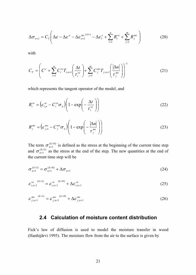
2.4 Calculation of moisture content distribution
Fick�s law of diffusion is used to model the moisture transfer in wood (Hanhijärvi 1995). The moisture flow from the air to the surface is given by

22
( )surfairn uuSq −= 0ρ (27)
where nq is the value of the flow across the boundary, 0ρ is the wood density in absolute dry conditions, S is the surface emissivity, airu is the equilibrium moisture content of wood corresponding to the air humidity and surfu is the moisture content on the wood surface.
The moisture transfer properties used here are the following:
( )75.0
46.6air
1101
1.647113.0
1ln01.0
−
−
⎟⎟⎟⎟⎟
⎠
⎞
⎜⎜⎜⎜⎜
⎝
⎛
⎟⎠⎞
⎜⎝⎛ −
−−=
T
TRHTu (28)
( )uS 4exp10.2.3 8−= m/s (29)
where T is the temperature in Kelvin degrees and RH is the relative humidity of the air.
The moisture transfer in wood is analogous to the transient heat conduction discribed by the Fourier law. This in not further defined in this work but can be easily found in the literature.
2.5 Material parameters
The material properties used in the calculations are as follows (Tables 1 and 2). These were obtained partially from earlier references and partially derived in the present study. Some of these have been adjusted to comply with earlier test results.

23
Table 1. Material properties used in the analysis.
Property number Notation Meaning
Value for
spruce
Value for
pine Unit
1 refrE , 600 900 MPa
2 reftE , 600 500 MPa
3 refzE ,
Elastic moduli at the reference configuration
12 000 12 000 MPa
4 rtν 0.558 0.558 -
5 rzν 0.038 0.038 -
6 tzν
Poisson’s ratios
0.015 0.015 -
7 refrtG , 40 40 MPa
8 refrzG , 700 700 MPa
9 reftzG ,
Shear moduli at the reference configuration
700 700 MPa
10 ru ,α Coefficient of moisture
expansion 0.13 0.13 -
11 tu ,α 0.27 0.27 -
12 zu ,α 0.005 0.005 -
13 0ρ Density at initial moisture content
450 550 kg/m3
14 0T Initial temperature 20 20 C!
15 0u Initial moisture content user user -
16 refρ Reference density 450 550 kg/m3
17 refT Reference temperature 20 20 C!
18 refu Reference moisture
content 0.2 0.2 -
19 1a Parameter related to
the density 0.0003 0.0003 m3/kg
20 1b Parameter related to
the temperature -0.007 -0.007 1/ C!
21 1c Parameter related to the moisture content
-2.6 -2.6 -
22 ve1τ
Retardation of the viscoelastic element
number 1 2.4 2.4 h

24
23 veJ1
Viscoelastic compliance of element 1 given as a factor of the elastic
compliance
0.085 0.085 -
24 ve2τ 24 24 h
25 veJ 2 0.035 0.035 -
26 ve3τ 240 240 h
27 veJ 3 0.07 0.07 -
28 ve4τ 2400 2400 h
29 veJ 4 0.2 0.2 -
30 ms1τ
Retardation of the mechanosorptive element number 1
0.01 0.01 -
31 TmsJ ,1
Compliance of the mechanosorptive
element number 1 in tangential direction
0.003 0.003 1/MPa
32 ZmsJ ,1
Mechanosorptive compliance of element 1 in longitudinal direction given as a factor of the elastic compliance at
reference configuration
0.035 0.035 -
33 ms2τ 0.1 0.1 -
34 TmsJ ,2 0.003 0.003 1/MPa
35 ZmsJ ,2 0.49 0.49 -
36 ms3τ 1 1 -
37 TmsJ ,3 0.07 0.07 1/MPa
38 ZmsJ ,3 0.25 0.25 -
39 vm Parameter for the
irrecoverable part of mechanosorptive creep
0.33 0.33 1/MPa

25
Table 2. Diffusion values used in the analysis (derived from Hanhijärvi 1995 and Sjödin 2006).
Moisture content of wood [-]
Radial diffusion coefficient
[m2/h]
Tangential diffusion
coefficient [m2/h]
Longitudinal diffusion
coefficient [m2/h]
0 0.0003888 0.0003888 0.0009
0.05 0.0004751 0.0004751 0.00504
0.055 0.0004841 0.0004841 0.00535
0.07 0.0005137 0.0005137 0.00567
0.085 0.0005461 0.0005461 0.00585
0.09 0.0005572 0.0005572 0.00567
0.135 0.0006690 0.0006690 0.00454
0.18 0.0008026 0.0008026 0.00307
0.23 0.0009690 0.0009690 0.00210
0.28 0.0012029 0.0012029 0.00135

26
3. Modelling of wood structures with ABAQUS
At present, there are no ready made wood models in ABAQUS for time dependent analysis, however there is a way to create own material models. ABAQUS uses several subroutines, programmed in FORTRAN language, to permit the user to define his own material model. In our case, it is necessary to use the UMAT subroutine to implement the rheological model of wood, and the DFLUX subroutine to define the flow of moisture on the surface of the wood. The following scheme (Figure 6) describes the modelling and calculating processes used for modelling wood in the present study.
Figure 6. Scheme of the wood modelling process.
ABAQUS CAE:
geometry, boundary conditions, material properties,
loads, mesh.
INPUT FILE:
geometry, boundary conditions, material properties,
loads, mesh.
UMAT SUBROUTINE:
rheological model: increment of stress
and tangent operator calculation
DFLUX SUBROUTINE:
moisture flow calculation.
ABAQUS/STANDARD:
moisture transfer, total strain increment and stress increment
calculation
OUTPUT FILE:
solution of the calculation

27
3.1 Modelling with ABAQUS CAE
As shown in the previous scheme (Figure 6), the user can define the geometry, the boundary conditions, the material properties, the (mechanical and humidity) loads and the mesh with ABAQUS CAE. Applying the following steps, it is possible to create a model of wood structure:
• Enter the part field,
! create the part(s), note that to create a glulam beam, it is recommended to first create the whole beam and then to divide it in several lamellae. This will avoid the discontinuities in results between lamella.
• Enter the property field,
! create the material(s); for the wood, create only the name, the material properties can be given directly in the input file by copy-pasting the material properties from the previous input file,
! create as many sections as materials in the structure, define which material is used for each section,
! attribute to each part of the structure the correspondent section,
! create a local cylindrical coordinate system for each piece of wood,
! attribute a material orientation for each piece of wood using the local cylindrical coordinate system.
• Enter the assembly field,
! instance the part and select all the parts of the structure, cross the option �independent�.
• Enter the step field,
! create as many step as needed for the load case, here select the kind of analyses, because the equations of thermal transfer and moisture transfer are analogous, select the coupled temperature-displacement analyses, then define the time period of the step, the maximum number of increment, the initial, minimum and maximum increment, the maximum temperature increment which corresponds to the maximum moisture increment in the moisture calculation case, define the kind of load (instantaneous or ramp),

28
! create a field output, select the results wanted in the output file and define the frequency of saving.
• Enter the interaction field (in case of contact between parts only),
! in case of glued parts, create a constraint, select the �Tie� constraint, and select the surfaces in contact,
! in case of sliding contact, create an interaction, select �surface to surface contact�, select the finer mesh or the stiffer material as master surface, select the option small sliding and then surface to surface (this option permits to adjust the geometry to avoid the initial overclosure), select the option �adjust only to remove overclosure� or create a set of surfaces to be adjusted (the slave surfaces for example) and use the option �adjust slave nodes in set�, select an interaction property or create one if necessary,
! create an interaction property, select �contact�, then, in the mechanical field, define the tangential and normal behaviour, for simple contact definition, it is recommended to use frictionless or penalty method for tangential behaviour, and hard contact for normal behaviour, select �allow separation after contact�.
• Enter the load field,
! create a field, this permits to define an initial moisture content, select the initial step, select the wood parts needed and give the initial moisture content magnitude ,
! create load, select the step and the kind of load, select �thermal� and �surface heat flux� to define the surfaces of moisture exchange between wood and air, select the �user defined� option, the magnitude has to be 1, it will then take the value calculated in the DFLUX subroutine,
! create a boundary condition, select the step and the kind of boundary condition needed,
! to define the initial moisture content, create a field, select the initial step, select the temperature option and select the whole part which has an initial moisture content to be defined, and then give its value,

29
! in case of contact analysis, it is strongly recommended to create a smooth amplitude for the loading, it will help the calculation to converge,
! some techniques can be used to facilitate the convergence of the analysis, see paragraph �Stability of the analysis� below.
• Enter the mesh field,
! seed the part instance,
! assign element type, use �coupled temperature displacement� family for transient analyses, it is recommended to use non-reduced quadratic element (C3D8T, C3D20T), they permit to obtain a more accurate moisture calculation,
! mesh the part instance.
• Enter the job field,
! create a job,
! in the job manager, create the input file, note that the input file will be saved in the ABAQUS work folder defined during the installation of the software.
At this stage the input file is created but not usable in this state, a few changes have to be done to link the input file to the subroutines.
3.2 Editing the input file
Before editing the input file, it is important to understand the file structure. The best way to do that is to understand the main key words used by ABAQUS. Usually, the keywords appear in this order in the input file:
*Node: all the nodes created for the mesh are defined at their initial position,
*Element: the elements are created using the node labels and the element type,
*Nset; *Elset; *Surface: the node sets, element sets and surface sets defined for the different load cases and boundary conditions are created,

30
*Material: for each material, this key word introduces the material definition. It may be coupled with some other keywords depending of the needs of the calculation,
*Boundary: definition of the boundary conditions,
*Initial conditions: definition of the initial conditions like initial moisture content for example,
*Step: this keyword introduces a step definition; there is one step definition for each step, and for each definition the load case and the outputs are defined.
To link the input file and the subroutines, it is necessary to modify the material and the step definitions. In the material definition, the material parameters have to be defined, for this it is necessary to use the following key words: *Conductivity, *Density, *Depvar, *Specific heat, *User material and define the required parameters. If the steps defined in the previous paragraph have been followed, it is only necessary to copy-paste the user material parameters from another input file, and then add *Field key word in the step definition:
*FIELD,NUMBER=1 surface_set_name, 0
In order to define the surface_set_name, find the keyword *INITIAL CONDITIONS and copy-paste the surface set name used for this option.
3.3 The user subroutines for ABAQUS
A subroutine here is a small algorithm written by the user in FORTRAN language. It uses ABAQUS state variables to calculate user�s variables and to modify the ABAQUS state variables if necessary. This algorithm runs in parallel to the ABAQUS solver. At each time increment there is an exchange of information between them.
For wood modelling, two subroutines are used: the UMAT and the DFLUX subroutines. The first one calculates the stress increment and the Jacobian matrix

31
for each time increment. The second one calculates the flow of moisture between the air and the wood surface.
The two following sections give some information about the state variables used and/or modified by the subroutines for wood modeling.
3.3.1 The UMAT subroutine
According to the ABAQUS documentation (ABAQUS 2003), the UMAT subroutine
• can be used to define the mechanical constitutive behaviour of the material
• can be used with any procedure that includes mechanical behaviour
• can use solution-dependent state variables
• must update the stresses and solution-dependent state variables to their values at the end of the increment for which it is called and must provide
the material Jacobian matrix εσ∆∂∆∂ , for the mechanical constitutive model.
For modelling wood, it is necessary to access and/or to modify the following variables at each time step (see chapter 2.3.):
STRESS: array of the stress vector at the beginning of the time step, must be updated in this routine to be the stress vector at the end of the time step,
DSTRAN: array of strain increments. If the *Expansion option (thermal expansion, not used in this case because the hygroexpansion is calculated in the UMAT subroutine) is used in the same material definition, these are the mechanical strain increments (the total strain increments minus the thermal strain increments),
DTIME: time step,
TEMP: temperature at the start of the time step. Here it is used as the moisture content at the start of the time step,

32
DTEMP: increment of temperature, here increment of moisture,
PROPS: array of material constants entered in the *User material option for the material. It refers to the material properties listed by the user in the input file,
STATEV: an array containing the solution-dependent state variables. These are passed in as the values at the beginning of the time step or these are updated in the user subroutines, in which case the updated values are passed in. In all cases STATEV must be returned as the values at the end of the time step. The size of the array is defined on the *Depvar option associated with this material,
DDSDDE: Jacobian matrix of the constitutive model εσ∆∂∆∂ , where σ∆ is the
stress increment and ε∆ is the strain increment. DDSDDE(I,J) defines the change in the Ith stress component at the end of the time step caused by an infinitesimal perturbation of the Jth component of the strain increment array.
The DFLUX subroutine
This subroutine will be called by the solver at each time step in order to calculate the moisture flow on the wood surface. Then, based on the result, the solver will be able to calculate the moisture transfer in the material using the diffusion parameters given in the input file.
User subroutine DFLUX
• can be used to define a flux as a function of position, time, temperature, element number, integration point number, etc. in a heat transfer or mass diffusion analysis
• ignores any AMPLITUDE references that may appear with the associated *Dflux or *Dsflux option
• uses the nodes for first-order heat transfer and mass diffusion elements as flux integration points.

33
The following state variables are used in the moisture transfer calculation:
FLUX: the magnitude of flux at this point. If the magnitude is not defined, FLUX(1) will be given as zero, this flux is not available for output purposes,
SOL: the estimated value of the solution variable (temperature in a heat transfer analysis or concentration in a mass diffusion analysis) at this time at this point,
TIME: current value of time (defined only in transient analysis).
The moisture diffusion property of wood is given in the input file with the key word *Conductivity.
3.4 Defining the relative humidity
There are two main ways to define the relative humidity in the DFLUX subroutine: creating an expression, which will give the relative humidity in function of the time, or giving a list of predefined relative humidity values for different times.
The first solution is very practical when defining cyclic relative humidity. Figure 7 shows the curve of a cycling relative humidity defined with a SINE function. In this case, the time function is the same for all the test period, only the amplitude and the mean value change in function of the time.
Relative humidity and load case
0
0.1
0.2
0.3
0.4
0.5
0.6
0 500 1000 1500 2000 2500
Time (h)
Load
(MPa
)
0.20.30.40.50.60.70.80.91
RH
Load (MPa) RH
Figure 7. SINE function used to define cycling of air relative humidity.

34
The second solution is suitable for example for monitored relative humidity as shown in Figure 8. In this case, the six hours measured values of relative humidity inside a building are given by the blue curve. The data are given in the subroutine by two variables, one for the time and one for the relative humidity. The data are given every six hours and the intermediate values are interpolated. This solution may make the DFLUX subroutine very big in size, which means that ABAQUS needs time to load it the first time, but after that it is very fast. The other solution is reading a text file containing the data from the DFLUX subroutine, but in this case, the file has to be opened at each increment of each node and this process is very heavy from the computational point of view and thus very slow.
0
10
20
30
40
50
60
70
80
90
100
0 28 56 84 112 140 168 196 224 252 280 308 336 364
Aika [vrk]
RH
[%]
0
2
4
6
8
10
12
14
16
18
20
u [%
]
RHulkRHsisu(ulk)u(sis)
tsis=20C
Figure 8. Example of monitored air relative humidity (Koponen 2002).
In both solutions, it is necessary to define the changes of relative humidity as smoothly as possible, especially for analysis with contact calculation. Instantaneous changes of relative humidity often create instabilities in the calculations.

35
3.5 Stability of the analysis
In order to facilitate the convergence of the analysis, a few alternative methods can be used. The most important is the smoothing of the applied loads, which includes the mechanical loads and the relative humidity. The ABAQUS Analysis User�s Manual (ABAQUS 2003) gives good advices about curves smoothing; refer to the chapter named �Amplitude curves� in this manual. It presents how ABAQUS changes an instantaneous load change into a ramp load change or into a so called smooth load change. The same methods can be used in the DFLUX subroutine to define the relative humidity. There are no precise rules on the use of smoothing technique, the only advice is that the more the analysis is complicated the more the load case has to be smoothed.
Another way to facilitate convergence of the calculations, in contact calculations particularly, is to start the analysis with a small time step and then increase it, if necessary. The critical point for the contact calculation is when the contact between two surfaces initiates, which corresponds generally to the time when the load is applied. If this load is applied smoothly and if the time step is small enough, the probability of convergence is much higher.
3.6 Running calculations using subroutines
When the input file and the subroutines are created, the calculation is run using a MS-Dos window with MS-Windows System or a command window with a UNIX or LINUX station. It is necessary to save the input file and the Fortran file in the same folder. The command to run the calculation is: ABAQUS job=input_file_name user=Fortran_file_name.
It is possible to add int at the end of this command line; it permits to display some informations in the command window for each increment.

36
4. Validation of the implementation
As a check of the used implementation, some simple cases have been modelled with ABAQUS CAE. The calculated results have been compared to earlier experimental results from literature.
All the following simulations use ABAQUS 6.5-3 and are run with ABAQUS/Standard. The hexagonal 3D elements C3D8T have been used to mesh the wood parts, 2D shell elements S3 and a rigid body option have been used to model the steel plate. The contacts have been modelled by a hard contact pair with a penalty method in the tangential direction using a 0.4 penalty factor.
Note that the purpose of these comparisons is to validate the methods used. The improvement of this model and of its parameters is a future task.
4.1 Test 1: constant load, moisture content and temperature
Since the mechanosorptive creep is solely moisture rate dependent, it is necessary to study constant moisture content cases to check the viscoelastic creep part of the model.
In this example (Figure 9), a wood cube has been loaded by a constant 5 MPa load in the longitudinal direction with constant moisture content (Relative Humidity 35%) and temperature (20ºC). The relative creep ( ) eltl / , (where ( )tl is the specimen�s length in function of the time and el is the elastic length after load application) has been monitored during a period of 1 year and has been compared to relative creep curves obtained by Leivo (1991) (Figure 10). For this calculation, Scots Pine material parameters were used.

37
Figure 9. Scheme and numerical model, constant 35% RH and constant 5 MPa load (125 elements).
Numerical tensil relative creep in grain
direction
1.01.11.21.31.41.51.6
0 100 200 300 400
Time (days) Figure 10. Relative creep, constant 35% RH and constant 5 MPa load, experimental results (Leivo 1991, Toratti 1992) and numerical results.
Measurement point
Leivo (1991)
Rel
ativ
e cr
eep
Time [days]
35% RH, 5 MPa 90% RH, 10 MPa
35% RH, 10 MPa Model 90% RH
90% RH, 5 MPa Model 35% RH
0 50 100 150 200 250 300 350 400
1.6
1.5
1.4
1.3
1.2
1.1
1

38
We can see from Figure 10 that the numerical viscoelastic relative creep in the longitudinal direction is the same order as the experimental results (see curve 35% RH 5 MPa).
4.2 Test 2: varying load and cyclic relative humidity, constant temperature
In test 2 (Figure 11) the experiments done by Svensson (1997a, b) have been used, where a small wood specimen has been loaded to a 0.5 MPa constant load during 168 hours in the tangential direction with a cyclic relative humidity and a constant temperature (20ºC). The load was removed for the next 168 hours. The strain was measured in the tangential direction. For this calculation, Scots Pine material parameters have been used, but the experimental results showed an unusual high stiffness, therefore the radial and tangential Young moduli were multiplied by two for this simulation. The free shrinkage strain has been substracted from both the tensile and the compressive strain results (shrinkage-corrected strain).
Figure 11. Test 2, scheme and numerical model (168 elements).

39
Relative humidity & load case
0
0.1
0.2
0.3
0.4
0.5
0.6
0 50 100 150 200 250 300 350
Time (h)
Load
(MPa
)
0.5
0.6
0.7
0.8
0.9
1RH
Load(Mpa) RH
TENSILE STRAINS: EXPERIMENTAL & NUMERICAL RESULTS
0.000
0.001
0.002
0.003
0.004
0.005
0.006
0.007
0 50 100 150 200 250 300 350Time (h)
TEN
SILE
STR
AIN
average experimental results numerical results exp1 exp5 exp13 exp17
TENSILE STRAINS: EXPERIMENTAL & NUMERICAL RESULTS
0.000
0.001
0.002
0.003
0.004
0.005
0.006
0.007
0 50 100 150 200 250 300 350Time (h)
TEN
SILE
STR
AIN
average experimental results numerical results exp1 exp5 exp13 exp17
Figure 12. Test 2, load case (stepwise RH and tension load), experimental results (average curve, exp1, exp5, exp13 and exp17 from Svensson 1997a) and numerical results.

40
The same test was done for a 0.5 MPa compressive load. The results are given in the Figure 13.
TENSILE STRAINS: EXPERIMENTAL & NUMERICAL RESULTS
-0.006
-0.005
-0.004
-0.003
-0.002
-0.001
0.0000 50 100 150 200 250 300 350
Time (h)
TEN
SILE
STR
AIN
average numerical results
Figure 13. Test 3, experimental results (average curve, from Svensson 1997b) and numerical results.
The results demonstrate (Figures 12 and 13) that the model gives good results in the tangential direction at least up to the second wetting cycle in the unloaded state. After the second wetting cycle, the recovering part is not complete as compared to the experimental results. Svensson (1997b) found the same behaviour of his model during the recovering time.
4.3 Test 3: varying load and cyclic relative humidity, constant temperature
In test 3, the experiments done by Svensson (1997a) have been used. The specimen geometry and the loading conditions are the same as for the test 2. The specimen was loaded to a 0.5 MPa constant tension load for 1400 hours in the tangential direction with a cyclic relative humidity and a constant temperature (20ºC). The load was removed for the next 900 hours. The strain was measured in the tangential direction in function of the time. The same material parameters have been used as in test 2. Figure 14 gives the results for this load case.

41
Relative humidity and load case
0
0.1
0.2
0.3
0.4
0.5
0.6
0 500 1000 1500 2000 2500
Time (h)
Load
(MPa
)
0.20.30.40.50.60.70.80.91
RH
Load (MPa) RH
TENSILE STRAINS: EXPERIMENTAL & NUMERICAL RESULTS
0
0.002
0.004
0.006
0.008
0.01
0.012
0 500 1000 1500 2000 2500
Time (h)
STR
AIN
exp 25 exp 26 exp 27 exp 28 exp 29 numerical results average experimental results
TENSILE RELATIVE CREEP: EXPERIMENTAL & NUMERICAL RESULTS
0
5
10
15
20
25
30
35
0 500 1000 1500 2000 2500
Time (h)
TEN
SILE
REL
ATI
VEC
REE
P
relative creep exp relative creep num exp 25 exp 26 exp 27 exp 28 exp 29
Figure 14. Test 3, load case (cycling RH and tension load), experimental results (average curves, exp1, exp5, exp13 and exp17 from Svensson 1997a) and numerical results.

42
The same test was done also for a 0.5 MPa compressive load. The results are given in the Figure 15.
COMPRESSIVE STRAINS: EXPERIMENTAL & NUMERICAL RESULTS
-0.014-0.012
-0.01-0.008-0.006-0.004-0.002
00 500 1000 1500 2000 2500
Time (h)
STR
AIN
exp1 exp2 exp3 Average numerical results
Figure 15. Test 3, experimental results (average curve, exp1, exp2 and exp3 from Svensson 1997a) and numerical results.
In both cases, tension and compression, the numerical results show good agreement with the experimental results. The global shape of the curves is the same and the values are very close.
4.4 Test 4: varying bending load and cyclic relative humidity, constant temperature
In test 4 (Figure 16) the experiments done by Leivo (1991) are used. In this case, a wood beam is loaded to a 10 MPa bending stress under cycling 35�90% relative humidity and a constant 20ºC temperature during one year. The deflection was measured. For this calculation, spruce (Picea abies) material parameters have been used.

43
Figure 16. Test 4, scheme and numerical model, beam 45 x 90 x 2000, bending stress 10 MPa (F = 1000 N), 70 days period cycling 35�90% relative humidity (7207 elements).

44
Computational relative creep: bending stress 10MPa
0.60.81.01.21.41.61.82.02.22.42.6
0 100 200 300
Time[days]
Figure 17. Test 4, relative creep, experimental (Leivo 1991, Toratti 1992) and numerical results.
Time [days]
Rel
ativ
e cr
eep
Bending stress 10 MPa
Computed results Test results
0 50 100 150 200 250 300 350
2.6
2.4
2.2
2
1.8
1.6
1.4
1.2
1
0.8
0.6

45
This bending test comparison has been done mainly to test the proposed model of wood in longitudinal direction. The results above (Figure 17) show that the numerical relative creep is close to the average of the experimental relative creep curves.
4.5 Test 5: calculation of moisture content and internal stresses in a glulam beam
This comparison case is used for studying the internal stresses perpendicular to grain in glued laminated (glulam) timber beams. The described beam section was experimentally analyzed by Jönsson (2005). The tested glulam beams (90 × 270, quality L40) contained six lamellae of Norway spruce. The glulam was sawn into 16 mm thick plates perpendicular to the beam axis, so that the specimens, free from knots, had the dimensions 16 × 90 × 270 mm.
The specimens were further sawn in eleven slices at a specific time and, on each slice, two markers were glued along each short side.
The wood boards were first seasoned at a constant relative humidity RH = 40% and constant temperature T = 20ºC during four months and then the relative humidity was changed to RH = 80% during 38 days. The results were given for each slice at the end of the four months and 38 days, respectively.
The length between markers was measured before and after sawing by an optical method. The mean stress was determined from the mean released strain for each slice:
meanmean uE εσ )(=
where the elastic modulus E(u), depending on the moisture content, was measured with a dynamic method. For the numerical simulation by ABAQUS, 396 quadratic elements C3D20T were used. Figure 18 shows the geometry of the Jönsson glulam beam section and the model analyzed by ABAQUS/Standard.
The computational results in terms of moisture content (Figure 19) and vertical stress (Figure 20), show a good agreement with the experimental data.

46
The 3D distribution of stresses and moisture are shown in Figure 21.
Figure 18. Jönsson�s glulam beam. Left: geometry of the beam. Right: ABAQUS model. (Jönsson 2005.)

47
Figure 19. Jönsson’s glulam beam. Results after 4 months drying. Average of the humidity per each slice. Comparisons between computational and experimental results. (Jönsson 2005.)
Figure 20. Jönsson’s glulam beam. Results after 4 months drying. Average of the vertical stress per each slice. Comparisons between computational and experimental results. (Jönsson 2005.)

48
Figure 21. Jönsson�s glulam beam. Results after 4 months and 38 days. Top: tangential stress in material coordinates. Center: tangential stress in global coordinates. Bottom: moisture distribution. (Jönsson 2005.)

49
5. Conclusions
A structural analysis model for the long-term response of wooden under variable load and humidity conditions has been developed with the finite element calculation software ABAQUS. The material properties of timber in the grain direction and in the perpendicular-to-grain directions require defining a local cylindrical coordinate system for each piece of wood of the structure, glulam for instance. The moisture transfer is composed of the moisture flow from the air to the wood surface and on the moisture diffusion in wood. The moisture flow has been implemented in a DFLUX subroutine. The response of wood to mechanical loading, moisture content changes and time was modelled by using a rheological model of wood implemented in an UMAT subroutine. Some simulations have been performed with this method. The comparisons to earlier experimental results from literature demonstrate that the implementation and models used function well.

50
References
ABAQUS version 6.4 documentation, 2003.
Dinwoodie, J. M. 1979. Timber, its nature and behaviour. Van Nostrand Reinhold.
Fortino, S., Hanhijärvi, A., Mirianon, F. and Toratti, T. 2008. A 3D Coupled Moisture-Stress Numerical Analysis for Timber Structures. Proceedings of the Joint IACM � ECCOMAS 2008 Conference, Venice (Italy), 30 June � 4 July 2008 (Joint IACM � IUTAM Minisymposium).
Hanhijärvi, A. 1995. Modelling of creep deformation mechanisms in wood. Espoo: Technical Research Centre of Finland, VTT Publications 231. 143 p. + app. 3 p. Dissertation.
Hanhijärvi, A. and Mackenzie-Helnwein, P. 2003. Computational analysis of quality reduction during drying of lumber due to irrecoverable deformation. i: Orthotropic viscoelasticmechanosorptive-plastic material model for the tranverse plane of wood. Journal of Engineering Mechanics, 129(9), pp. 996�1005.
Jönsson, J. 2005. Moisture Induced Stresses in Timber Structures. Dissertation. Report TVBK-1031. Division of Structural Engineering. Lund University of Technology.
Koponen, S. 2002. Puurakenteiden kosteudenhallinta rakentamisessa. Raportti 1-0502. Teknillinen Korkeakoulu. (In Finnish.)
Leivo, M. 1991. On the stiffness changes in nail plate trusses. Espoo: Technical Research Centre of Finland, VTT Publications 80. 190 p. + app. 46 p. Dissertation.
Mackenzie-Helnwein, P. and Hanhijärvi, A. 2003. Computational analysis of quality reduction during drying of lumber due to irrecoverable deformation. ii: Algorithmic aspects and practical application. Journal of Engineering Mechanics, 129(9), pp. 1006�1016.

51
Ormarsson, S. 1999. Numerical analysis of moisture-related distorsions in sawn timber. Chalmers University of Technology. Dissertation.
Santaoja, K., Leino, T., Ranta-Maunus, A. and Hanhijärvi, A. 1991. Mechano-sorptive structural analysis of wood by the ABAQUS finite element program. Espoo: Technical Research Centre of Finland, Research Notes 1276. 33 p. + app. 16 p.
Sjödin, J. 2006. Steel-to-timber dowel joints � influence of moisture induced stresses. Växjö University. Licentiate Thesis.
Svensson, S. 1997a. Internal Stress in Wood Caused by Climate Variations. Lund Institute of Technology. Dissertation.
Svensson, S. 1997b. Mechano-Sorptive Behaviour of Wood Perpendicular to Grain. International Conference on Wood-Water Relations, COST Action E8. Pp. 309�324.
Toratti, T. 1992. Creep of timber beams in a variable environment. Helsinki University of Technology, Report 31. Dissertation.


Series title, number and report code of publication
VTT Publications 687 VTT-PUBS-687
Author(s)
Mirianon, Florian, Fortino, Stefania & Toratti, Tomi Title
A method to model wood by using ABAQUS finite element software Part 1. Constitutive model and computational details Abstract A structural analysis method for the long-term response of wood structures is presented in this report. This method has been developed with the finite element calculation software ABAQUS and its use requires
− an effective computer
− an ABAQUS licence
− a Fortran licence compatible with the ABAQUS CAE version
− the implementation scheme of the stress-strain relation for wood into the FE-program (UMAT subroutine for ABAQUS)
− the implementation of the equation for moisture flow across the wood surface (DFLUX subroutine for ABAQUS).
The forth and fifth components of the list above have been developed at The Technical Research Centre of Finland VTT. The material properties of timber in the grain direction and in the perpendicular-to-grain directions require defining a local cylindrical coordinate system for each piece of wood of the structure. The moisture transfer in wood is a function of the moisture flow on the wood surface and on moisture diffusion of wood. The response of wood to mechanical loading, moisture content changes and time was modelled by using a rheological model of wood implemented in a subroutine. The use of ABAQUS for detailed stress analyses of wood is demonstrated with examples.
ISBN 978-951-38-7107-9 (URL: http://www.vtt.fi/publications/index.jsp)
Series title and ISSN Project number
VTT Publications 1455-0849 (URL: http://www.vtt.fi/publications/index.jsp)
17546
Date Language Pages August 2008 English, Finnish abstr. 51 p.
Name of project Commissioned by Improved glued wood composites – modelling and mitigation of moisture-induced stresses
Tekes, woodwisdom-net programme
Keywords Publisher timber, gluelam, moisture transfer, stress analysis, FEM, ABAQUS, creep, mechano-sorption, deformation, humidity
VTT Technical Research Centre of Finland P.O. Box 1000, FI-02044 VTT, Finland Phone internat. +358 20 722 4404 Fax +358 20 722 4374


Julkaisun sarja, numero ja raporttikoodi
VTT Publications 687 VTT-PUBS-687
Tekijä(t) Mirianon, Florian, Fortino, Stefania & Toratti, Tomi Nimeke
Puun mallintaminen käyttäen ABAQUS-elementtimenetelmäohjelmistoa Osa 1. Konstitutiiviset mallit ja analyysimenetelmä
Tiivistelmä Työssä kehitettiin analyysimenetelmä puurakenteiden pitkäaikaisominaisuuksien arviointiin. Malli tehtiin elementti-menetelmällä käyttäen ABAQUS-ohjelmistoa. Mallin käyttö edellyttää
− tehokasta tietokonetta
− voimassa olevaa ABAQUS-lisenssiä
− Fortran-kääntäjää, joka on yhteensopiva ABAQUS CAE -version kanssa
− käyttäjän ohjelmoimaa puun jännitys-venymä-kosteusmallia, jota sovelletaan ABAQUS-elementti-menetelmäohjelmassa (aliohjelmat UMAT ja DFLUX).
Puun rakenne- ja materiaaliominaisuudet syyn suunnassa ja syitä vasten kohtisuorassa edellyttävät sylinterimäistä koordinaatistoa puun mallintamiseksi. Kosteuden siirtyminen on mallitettu pintaemissiolla ilmasta puuhun sekä diffuusio siirtymisenä puun sisällä. Analyysi perustuu reoloogiseen malliin, jossa mekaaninen kuorma, kosteus ja ajasta riippuvat vaikutukset on mallitettu ABAQUS-ohjelmistoon sisällytettävillä aliohjelmilla.
ABAQUS CAE -ohjelmiston käyttö puun rakenneanalyysissä esitetään yksityiskohtaisesti. Lisäksi mallin antamia tuloksia verrataan joihinkin aikaisempiin koetuloksiin.
ISBN 978-951-38-7107-9 (URL: http://www.vtt.fi/publications/index.jsp)
Avainnimeke ja ISSN Projektinumero VTT Publications 1455-0849 (URL: http://www.vtt.fi/publications/index.jsp)
17546
Julkaisuaika Kieli Sivuja Elokuu 2008 englanti, suom. tiiv. 51 s.
Projektin nimi Toimeksiantaja(t) Improved glued wood composites – modelling and mitigation of moisture-induced stresses
Tekes, woodwisdom-net programme
Avainsanat Julkaisija
timber, gluelam, moisture transfer, stress analysis, FEM, ABAQUS, creep, mechano-sorption, deformation, humidity
VTT PL 1000, 02044 VTT Puh. 020 722 4404 Faksi 020 722 4374

VTT P
UB
LICA
TION
S 687 A
method to m
odel wood by using A
BA
QU
S finite element softw
are. Part 1. Constitutive...
ESPOO 2008ESPOO 2008ESPOO 2008ESPOO 2008ESPOO 2008 VTT PUBLICATIONS 687
Florian Mirianon, Stefania Fortino &Tomi Toratti
A method to model wood by usingABAQUS finite element software
Part 1. Constitutive model and computationaldetails
A structural analysis method for the long-term response of woodstructures is presented in this report. The method has been developed forthe finite element calculation software ABAQUS applying a user definedmaterial model. The response of wood to mechanical loading, moisturecontent changes and time was modelled by using a rheological model ofwood. The use of ABAQUS CAE for detailed stress analyses of wood isdemonstrated with examples.
ISBN 978-951-38-7107-9 (URL: http://www.vtt.fi/publications/index.jsp)ISSN 1455-0849 (URL: http://www.vtt.fi/publications/index.jsp)
VTT VTT VTTPL 1000 PB 1000 P.O. Box 1000
02044 VTT 02044 VTT FI-02044 VTT, FinlandPuh. 020 722 4520 Tel. 020 722 4520 Phone internat. + 358 20 722 4520
http://www.vtt.fi http://www.vtt.fi http://www.vtt.fi
Recommended