MIT
Delay Models and Queueing
Muriel MedardEECSLIDSMIT

MIT
Outline• Introduction• Concepts of ergodicity• Little’s theorem• Application: Pollaczek-Khinchin• Poisson process• Markov overview• M/M/… systems• Review of transforms• M/G/… systems• Extensions of Markov approach to non M/M/ systems• Reverse chains• Burke’s theorem for reversibility• Networks of queues• Kleinrock’s independence assumption• Jackson’s Theorem
MIT
The importance of queues
• When do queues appear?– Systems in which some serving entities provide some service in a
shared fashion to some other entities requiring service• Examples
– customers at an ATM, a fast food restaurant– Routers: packets are held in buffers for routing– Requests for service from a server or several servers– Call requests in a circuit-oriented system such as traditional
telephony, mobile networks or high-speed optical connections

MIT
What questions may we want to pose?
• What is the average number of users in the system? What is theaverage delay?
• What is the probability a request will find a busy server?• What is the delay for serving my request? Should I upgrade to a
more powerful server or buy more servers?• What is the probability that a packet is dropped because of
buffer overflow? How big do I need to make my buffer tomaintain the probability of dropping a packet below somethreshold? What is the probability that I cannot accommodate acall request (blocking probability)?
• For networked servers, how does the number of requests queuedat each server behave?
• We shall keep these types of questions in mind as we go forward

MIT
Analysis versus simulation
• Why can’t I just simulate it?• Analysis and simulation are complementary, not opposed• It is generally impossible to simulate a whole system- we
need to be able to determine the main components of thesystem and understand the basis for their interaction
• What are the important parameters? What is their effect?• In many systems simulation is required to qualify the results
from analysis, to obtain results that are too complexcomputationally

MIT
Delay components
• Processing delay: for instance time from packet reception toassignment to a queue (generally constant)
• Queueing delay: time in queue up to time of transmission• Transmission delay: actual transmission time (for instance
proportional to packet length)• Propagation delay: time required for the last bit to go from
transmitter to receiver (generally proportional to the physicallink distance, large for satellite link) [Not to confuse withlatency, which is number of bits in flight, latency goes upwith data rate] queueing
processing
transmission

MIT
Little’s theorem
• Rather than refer to packets, calls, requests, etc… we refer tocustomers
• Relates delay, average number of customers in queue andarrival rate (λ)
• Little’s Theorem: average number of customers = λ xaverage delay
• Holds under very general assumptions

MIT
Main parameters of a queueing system
• N(t): number of customers in the system at time t• P(N(t) = n) = probability there are n customers in the system
at time t• Steady state probability:
• Mean number in system at time t:
• Time average number in the system:
• We assume the system is ERGODIC:
n)P(N(t)limP tn == !"
MIT
Main parameters
• We looked at the system from the point of view of the customers init, let us now consider the delay of those customers
• T(k): delay of customer k• α(t): number of customer arrivals up to time t• β(t): number of customer arrivals up to time t• Our ergodicity assumption implies that the long-term arrival rate is
the long-term departure rate:
• Our ergodicity assumption implies that there exists a limit:

MIT
Little’s theorem
• We have:
• Little’s theorem applies to any arrival-departure system withappropriate interpretation of average number of customers in thesystem, average arrival rate and average customer time in system

MIT
Justification of Little’s theorem
T(1)
T(2)
T(3)
t
T(4)
T(5) T(5)
Note: a similar picture holds even if we do not have FIFO
T(1)
T(2)
T(3)
T(4)
T(1)
T(2)
T(3)
T(4)
T(5)

MIT
Justification of Little’s theorem
• Taking the average over time:
Goes to T in the limit as t → ∞
Goes to λ in the limit as t → ∞

MIT
Example of application
• Applying Little’s theorem to the queueing portion to obtainthe average number waiting in queue
• Applying Little’s theorem to the transmission portion todetermine the proportion of time transmission is occurring:
queueing transmission

MIT
Application to complex systems
• Suppose we have several different traffic streams• Applying to each traffic stream yields• Applying to all M streams collectively:
• We have answered the first question insofar as we candetermine N from T or T from N, but we need moreinformation to determine both

MIT
Pollaczek-Khinchin
• General type of service times, X is the service time, withmeans E[X] and E[X2] known
• Arrivals are memoryless: arriving customer in steady-statesees mean behavior
• The main formula is the Pollaczek-Khinchin formula (P-K)for the waiting time W in queue

MIT
Examples
• Nomenclature for queues:Arrival type/Service type/Number of servers/Buffer size
• Common types: M (Poisson distributed), G (general), D(deterministic)
• M/M/1: P-K gives
• M/D/1: deterministic service time where every user has equalservice time 1/µ, P-K gives
• P-K is a M/G/1 formula

MIT
Proof of P-K
• W(k): waiting time in queue of customer k• R(k): residual service of customer k• X(k): service time of customer k• N(k): number of customer found waiting in queue by
customer k (memoryless assumption)
Using Little’s theorem

MIT
Residual time
• We have reduced everything in terms of R• Let r(t) be the residual time at time t,• Let M(t) be the customer completing service at time t
r(t)
tX(1)
X(1)
X(2)

MIT
Residual time
• By looking at the area we consider:

MIT
Priorities
• The M/G/1 model will help us understand priorities• Priorities 1,.., k, with 1 being the highest• λ(k), µ(k): arrival and service rates of priority k• W(k): average queuing time for priority k• ρ(k) = λ(k)/ µ(k): utilization factor for priority k• R: mean residual time• Let us look at preemptive priority:
– customer in service is interrupted by an arriving higherpriority customer
– Interrupted customer resumes service from the point ofinterruption

MIT
Preemptive priority
• For preemptive priority:
• Higher priority users do not “see” lower priority users

MIT
Non-preemptive priority
• Customer in service is not interrupted, so W for low prioritywill depend on high priority
• Assuming <1

MIT
What questions may we want to pose?
• What is the average number of users in the system? What is theaverage delay?
• What is the probability a request will find a busy server?• What is the delay for serving my request? Should I upgrade to a
more powerful server or buy more servers?• What is the probability that a packet is dropped because of
buffer overflow? How big do I need to make my buffer tomaintain the probability of dropping a packet below somethreshold? What is the probability that I cannot accommodate acall request (blocking probability)?
• For networked servers, how does the number of requests queuedat each server behave?
• We shall keep these types of questions in mind as we go forward

MIT
M/M/1 system
• Poisson process A(t) with rate λ is a probabilistic arrivalprocess such that:– number of arrivals in disjoint intervals are independent– number of arrivals in any interval of length τ has Poisson
distribution with parameter λτ:
Memoryless arrival
Memoryless service time
Single server

MIT
Poisson process
• The distribution of the time Yk of the k th arrival has anErlang probability density function:
k=1
k=2
k=3
y
fY (y)k

MIT
Further properties of the Poisson process
• Interarrival time τ(n) for interarrival between nth and (n+1)st
arrival. The interarrival times are independent andexponentially distributed with parameter λ:
• For very small δ, we can say that:
0 as 0 )o(
where
)o()2A(t))P(A(t
)o()1A(t))P(A(t
)o(1)0A(t))P(A(t
!!
="#+
+==#+
+#==#+
$$
$
$$
$%$$
$%$$
τ(n)
MIT
Further properties of the Poisson process
• We can condition on any past history, the time until the nextarrival is always exponentially distributed, hence the termmemoryless
• If A1, A2, …, Ak are independent Poisson processes withrates λ1, λ2, …, λk then the process A = A1+ A2+ …+Ak isPoisson with rate λ = λ1+ λ2+ …+λk
• Poisson processes are generally a good model for thecollective traffic of a large number of small users

MIT
Further properties of the Poisson process
• Probabilistic splitting of Poisson processes is Poisson
• What is probability that last arrival was from the top process?
λ
λp
Bernoulli pλ(1−p)
MIT
M/M/1
• Single server• Poisson arrival process with rate λ• Independent identically distributed (IID) service times X(n) for the
service time of user n• Service times X are exponentially distributed with parameter µ, so
E[X] = 1/µ• Interarrival times and service times are independent• We define ρ = λ /µ, we shall see later how that relates to the ρ we
considered when discussing Little’s theorem• Can we make use of the very special properties of Poisson
processes to describe probabilistically the behavior of the system?

MIT
Derivation of occupancy distribution
• Let us make use of the small δ approximation• In a small δ interval, we have probability roughly λδ of
having an arrival and 1 - λδ of having no arrival• If there is a customer in the system, then we have probability
roughly µδ of having a departure and 1 - µδ of having nodeparture
• Markov chain:state is number in the system
0 1 2 n-1 n n+1...
µδ µδ µδ µδ µδ µδ
λδλδλδλδλδλδλδ
µδ

MIT
Markov chain for M/M/1
• In steady state, across some cut between two states, theproportion number of transitions from left to right must bethe same as the proportion of transitions from right to left
• Local balance equations, consider steady-state and replaceN(t) with N
0 1 2 n-1 n n+1...
µδ µδ µδ µδ µδ µδ
λδλδλδλδλδλδλδ
µδ

MIT
Balance equations
• We know that
• Let us use this fact to determine all the other probabilities
• We have
• Let us answer the second question:– we use the fact that Poisson arrivals see time average (PASTA)– the probability of having a random customer wait is ρ

MIT
Mean values
• We can now make use of Little’s theorem to answer our firstset of questions:
• What is the wait in queue, ? Use independence of servicetimes to get = - 1/µ

MIT
More queue scenarios
• A similar type of analysis holds for other queue scenarios:– set up a Markov chain– determine balance equations– use the fact that all probabilities sum to 1– derive everything else from there
• M/M/m queue: Poisson arrivals, exponential distribution ofservice time, m servers
• Similar analysis to before, except now the probability of adeparture is proportional to the number of servers in use,because a departure occurs if AT LEAST one of the servershas a departure
• Now ρ = mµ − union bound holds for first order

MIT
Markov chain for M/M/m
0 1 2 m-1 m m+1...
µδ 2µδ 3µδ mµδ mµδ mµδ
λδλδλδλδλδλδλδ
(m−1)µδ

MIT
Let us answer our first two questions
• Second question, what is the probability that a customer mustwait in queue:Erlang C formula
• Applying Little’s theorem:

MIT
One server or many?
• We now have the tools to answer our third question: would I ratherhave a single more powerful server or many weaker servers?
• Would we rather have a single server with service rate mµ or mservers with service rate µ? Related question: if we have somechannel do we want to allow statistical multiplexing onto m equalsubchannels or not?
• For light loads, the delay is roughly m times for the system withseveral server channels
• For heavy loads, the delays are about the same

MIT
M/M/∞
• Infinite number of servers• Taking m to go to ∞ in the M/M/m system, we have that the
occupancy distribution is Poisson with parameter λ/µ
• = 1/µ

MIT
Finite-storage: M/M/1/K
• Fourth question
• PASTA yields probability that a new call is blocked
0 1 2 K-1 K...
µδ µδ µδ µδ
λδλδλδλδλδ
µδ

MIT
Another example of finite storage: M/M/m/m
• Limited number of servers, no place to queue
• Answer to fourth question is P(N=m), called Erlang B formula
0 1 2 m-1 m...
µδ 2µδ 3µδ mµδ
λδλδλδλδλδ
(m−1)µδ

MIT
Different distributions
• Suppose we want to consider arrival and departure processthat are not exponential
• Simplest extension: bulk arrivals• We can easily generalize the M/M approach to Erlang
distributions - this is the method of stages• We can consider that we need k stages to establish a single
arrival or departure• We attempt to match the distribution to the closest Erlang, Ek
k=1
k=2
k=3
y
fY (y)k
MIT
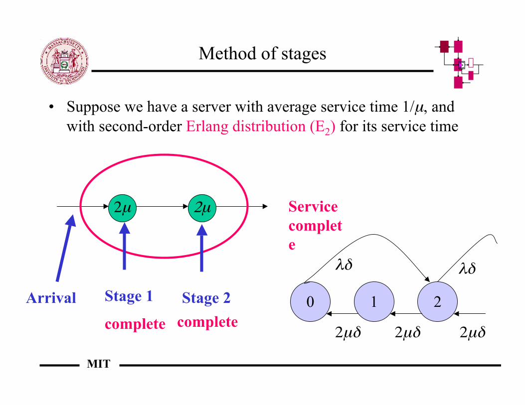
Method of stages
• Suppose we have a server with average service time 1/µ, andwith second-order Erlang distribution (E2) for its service time
2µ 2µ
Arrival Stage 1 Stage 2complete complete
Servicecomplete
0 1 2
2µδ 2µδ 2µδ
λδλδ
MIT
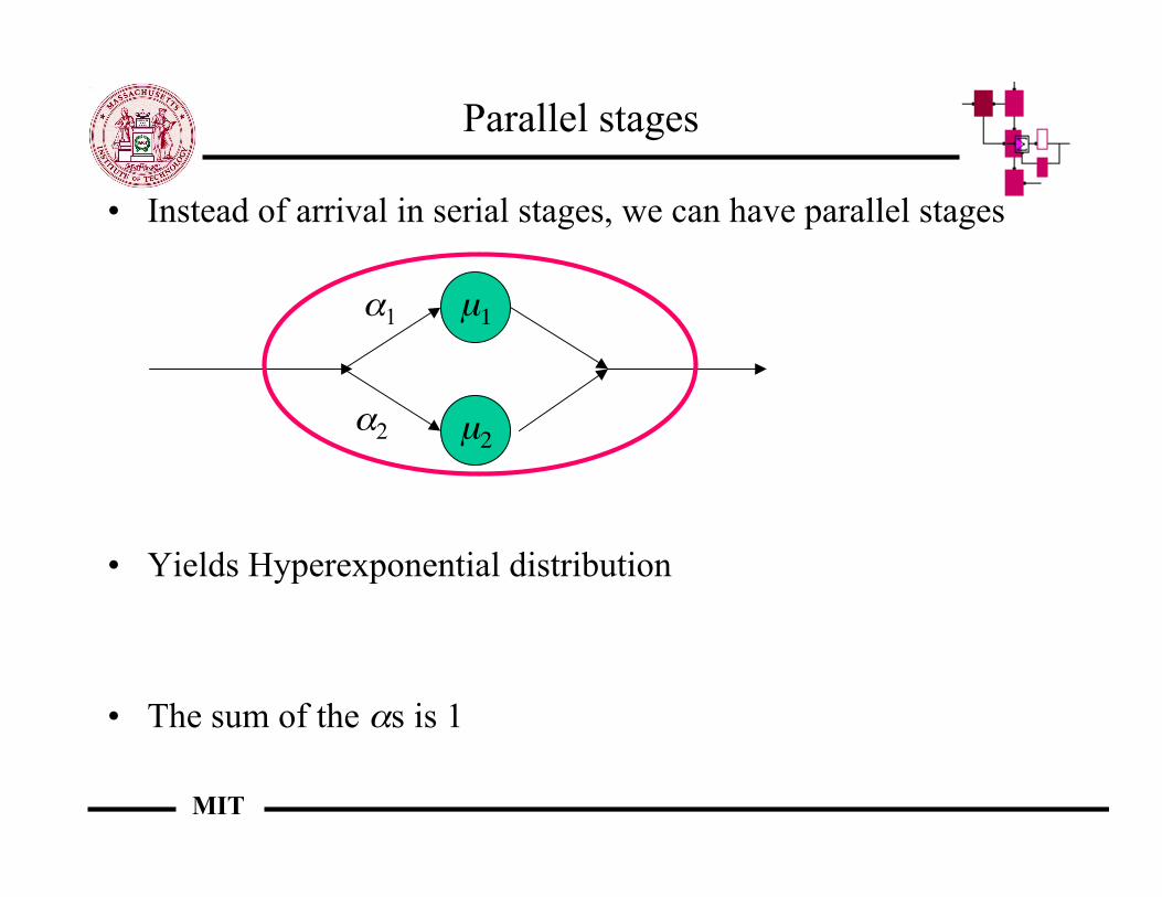
Parallel stages
• Instead of arrival in serial stages, we can have parallel stages
• Yields Hyperexponential distribution
• The sum of the αs is 1
µ1
µ2α2
α1

MIT
Beyond extensions to M/M/...
• The typicality of the state seen by an arrival is predicated onPASTA, so the M/ part is very powerful
• The assumption of memoryless arrivals is more commonly validthan the assumption of exponentially distributed service
• Extensions of the M/ ?/ using variations on the memorylessdistribution become increasingly complicated
• More advanced approach: M/G/1 queues
MIT
Transform review
• Transform is a function of a parameter z or s• Transform is well-defined for• We define the z-transform for discrete random variable V and
the Laplace transform for the continuous random variable B as:

MIT
Transform review
• Properties of transforms:

MIT
Transform review
• Sums of independent random variables: the transform of thesum is the product of the transform
• Random sum of random variables:
• Can derive compute transforms, manipulate in the transformdomain, then derive distribution using inverse transform
( )( )sBVB
BV
V
k
k
k
* is of transformthe
variablesrandom IID be Let there
0
!=

MIT
Transform review
• Example: sum of independent Gaussian random variables isGaussian
( )( )
( ) [ ] ( )
( ) ( ) ( ) ( )
( )( )21
2
2
2
1
2
2
2
2
2
1
2
1
2
22
2
2
2
22
2121
2
2
.
*.**
*
2
1
µµ!!
µ!
µ!
µ!
!
µ
"!
+#$$
%
&
''
(
) +
#$$
%
&
''
(
)#$$
%
&
''
(
)
#$$
%
&
''
(
)
##
##
=
=
=+
===
=
*
ss
ss
ss
ss
X
x
sxsX
i
x
i
X
e
ee
sXsXsXX
edxxfeeEsX
exf
ii
i
i
i
i
i

MIT
M/G/1 queue occupation
• Recall that PASTA holds• Case when a departing customer leaves a non-empty queue
server
queue
Customer n
Customer n
Customer n+1
Xn
Customer n+1
Customer n
Qn in queueCustomer n+1
Xn+1
Qn+1 in queue
Vn+1 arrivals

MIT
M/G/1 queue occupation
• Recall that PASTA holds• Case when a departing customer leaves an empty queue
server
queue
Customer n
Customer n
Xn
Customer n Customer n+1
Xn+1
Qn+1 in queue
Vn+1 arrivals
Customer n+1
Customer n+1
empty

MIT
Difference equations
• We can express the events in a difference equation
because the number of arrivals is independent of the past (Poisson)
[ ] [ ][ ] [ ] [ ]11
11
)(
00
01
0
01
11
1
1
1
++
++
!"+!"
+!"
++
+
+
+
==
=#
$%&
=
>=!
+!"=
$%&
=
>+"=
nnQnnnQn
nnQnn
n
VQVQ
n
VQQ
n
k
nQnn
nn
nnn
n
zEzEzEzQ
zEzE
k
k
VQQ
QV
QVQQ

MIT
Difference equations
• Use the steady-state assumptions
[ ][ ]
[ ] ( )
( ) ( )
( ) ( ) ( )011
0
0
)()(
)(
0
1
1
0
1
1
=!=+==
=+==
==
="
=
#
#
#
$
=
$
=
!
$
=
%!%!
%!
+
+
nnk
k
n
nk
k
n
nk
kQ
Q
n
V
QPz
kQPzz
QP
kQPzQP
kQPzzE
zVzEzQ
zVzE
knQn
nQn
n

MIT
Difference equations
• Use the steady-state assumptions again
• How do we relate this to the service time?
( )
( )z
zV
zzVzQ
z
QPzQQPzVzQ
zQzQn
!
"#
$%&
'!!
=(
"#
$%&
' =!+==(
=+
1
111
)()(
)0()()0()()(
)()(1
)

MIT
Service time and V
• Again use PASTA( )
( )
( )
( ) ( )
)(*
!)(
0
0
0 0
zX
dxxfe
dxxfee
dxxfk
xzezV
X
xz
X
xzx
Xk
k
x
!!
!
!!
!!
!
"=
=
=
##$
%&&'
(=
)
)
) *
+""
+"
+ +
=
"

MIT
P-K transform equation
• P-K transform equation
• Check: M/M/1
same as for N!
( )( )zzX
zzXzQ
!!
!!!=
)(*
11)(*)(
""
#""
( )( )
kkQP
zz
z
z
zzQ
ssX
!!
!
!
""µ
µ
!
""µ
µ
µ
µ
)1()(
1
111)(
)(*
#==$
#
#=
#%&
'()
*
#+
##
#+=
+=

MIT
M/M/x queues
• Markov chains:
0 1 2 n-1 n n+1...
µδ µδ µδ µδ µδ µδ
λδλδλδλδλδλδλδ
µδ
0 1 2 m-1 m m+1...µδ 2µδ 3µδ mµδ mµδ mµδ
λδλδλδλδλδλδλδ
(m−1)µδ
0 1 2 m-1 m m+1...
µδ 2µδ 3µδ mµδ (m+1)µδ mµδ
λδλδλδλδλδλδλδ
(m−1)µδ
M/M/1
M/M/m
M/M/∞

MIT
Steady-state distribution
• Use Markov property: denote in steady-state
( )
( )( )
( ) ( )( ) ( )
( )( )
( ) ( )( )
j
iji
k
k
k
k
k
p
Pp
imNP
jmNimNPjmNP
imNP
imNjmNP
imNikmNimNPimNP
imNjmNikmNimNPimNjmNP
ikmNimNimNP
ikmNimNimNjmNP
ikmNimNimNjmNP
,
2
2
2
2
2
)1(
)(|)1()(
)1(
)1(,)(
)1(|)(,...,)2()1(
)1(,)(|)(,...,)2()1(,)(
)(,...,)2(,)1(
)(,...,)2(,)1(,)(
)(,...,)2(,)1(|)(
=
=+
==+==
=+
=+==
=+=+=+=+
=+==+=+=+==
=+=+=+
=+=+=+==
=+=+=+=
))(|)1((),(,
ikNjkNPPiNPpiji
==+===

MIT
Reverse chain
• Let us consider a chain where the transition probabilities are:
• Steady-state probabilities:
• Hence,
i
ijj
ji
p
PpP
,
,* =
j
ji
jj
i
j
jii
jj
ijjj
i
p
Ppp
p
PppPpp
,
0
,
0,
0
***** !!!"
=
"
=
"
=
===
1***,
0,
0,
0,
0
=!=== """"#
=
#
=
#
=
#
=ji
jji
jiji
j
i
jj
ijjj
iPPpP
p
ppPpp
iipp *=

MIT
Burke’s theorem and reversibility
• Burke’s theorem: consider an M/M/1, M/M/m or M/M/∞ systemwith arrival rate λ. Suppose that the system starts in steady-state.Then:– The departure process is Poisson with rate λ– At each time t, the number of customers in the system is
independent of the sequence of departures prior to t• Proof:
– For the first part of the theorem, note that the forward andreversed systems are statistically indistinguishable in steady-state
– The departures prior to t in the forward process are also thearrivals after t in the reversed system and the arrival process inthe reversed system is independent Poisson

MIT
Burke’s theoremForward system Reversed system
Number of arrivals
time
a1 a2 T
d1 d2T
Number of departures
Number in system
a1 a2 d1 d2
Number of arrivals
time
T-d2 T
T
Number of departures
Number in system
T-d1
T-a2 T-a1

MIT
Networks of queues
• Closed form solutions are difficult to obtain• Poisson with feedback does not remain Poisson
λ
Poisson Poisson Poisson
λ
Poisson
NOT POISSON

MIT
Network of queues
• Several streams, each on a path p, each with rate λ(p)• Let us look at directed link (i,j):
j)(i,link on packets ofnumber averagej)N(i,
j)(i,link on rate servicej)(i,
(p)j)(i,j)(i,link g traversinp paths all
=
=
= !
µ
""

MIT
Kleinrock independence assumption
• Assume all queues behave like M/M/1 with arrival rate λ(i,j),service rate µ(i,j), and service/propagation delay d(i,j)
• Then
!
!
=
=
+"
=
pp
ji,ji,
ji,ji,ji,ji,
ji,ji,
NT
theorem)sLittle' (using system in the timeaverage
NN
network wholein the packets ofnumber average
dN
#
##µ
#

MIT
How good is it?
• Good for densely connected networks and moderate to heavyloads
• Good to guide topology design before involving simulation,other applications where a rough estimate is needed
• Other methods involve G/G/m approximations, using firstand second moments of interarrival and service times
• Are there any networks of queues where we can establishanalytical results?

MIT
Reversibility in Markov queues
• Consider a reversed chain: reversibility exists iff the detailedbalance equations hold
• Reversed chain :– Reversed chain is irreducible, aperiodic and has the same
stationary distribution as the forward chain– If we can find positive pi numbers that sum to 1 such that
ij
jiij
ijj
ji
i
jji
i
ijj
ji
pPpPp
P
p
Pp
PpP
==
==
!!
!
,,
,
,
,
,
* :Note
chain reversed theof iesprobabilitn transitio theare s*
theand onsdistributi stationary theare s the
then1*satisfy *

MIT
Jackson’s theorem
• Assuming that:– arrival processes from outside the network are Poisson– at each queue, streams have the same exponential service time
distribution and a single server– interarrival times and service times are independent
• Then:– the steady state occupancy probabilities in each queue are the
same as if the queue were M/M/1 in isolation• These results can be extended to:
– state-dependent service rates (for instance M/M/m queues)– closed networks

MIT
Jackson’s Theorem
• Model: K queues
• Jackson’s Theorem:
ji ,!
Queue i
ik ,!
Queue ji
µ
ir
jiii
jjr
,1
!"" #$
=
+=
iN
j
j
j
µ
!" =
( )
( ) )(
and 1)(
1ii
K
i
i
n
iii
nNPnNP
nNPi
===
!==
"=
rr
##

MIT
Jackson’s Theorem
• Some definitions:
( )( )
!!
"
#
$$
%
&
+'+'=
(
!!
"
#
$$
%
&
+'=
(
!!
"
#
$$
%
&
+'=
(
+'
'
+
=
==
'+
'
+
Kjjjiiiji
Kjjjj
Kjjjj
nn
nn
nnnnnnnnnn
nnnnnnn
nnnnnnn
nNP
PnNPP
,...,,1,,...,,1,,...,,
,...,,1,,...,,
,...,,1,,...,,
'*
111121,
1121
1121
,'
',
r
r
r
rr
rrrr
rr
Exogenous
Endogenous

MIT
Jackson’s Theorem-Proof Technique
• Establishing the balance equations is difficult because ofdifferent types of transitions
• We assume the answer• Using this answer, we see whether the forward and reverse
system check out• From the statement of Jackson’s Theorem, we have that:
( ) ( )( ) ( )!+
+
===
===
ji
ji
j
j
nNPnNP
nNPnNP
,rrrr
rrrr
""
"

MIT
Exogenous arrivals/departures
• Transition probabilities for both chains
( )
( ) ( )
( )
j
j
jnn
K
iijjnn
j
j
K
iijjnn
jnn
rP
P
nNPnNP
P
rP
j
j
j
j
!
µ"
"#!
$
"#µ
"
=
%=
===
%=
=
%
+
+
%
+
&
&
=
=
rr
rr
rr
rr
rrrr
,
1,,
1,,
,
*
1*
:assumptionour By
1

MIT
Endogenous arrivals/departures
• Transition probabilities for both chains
( ) ( )
ij
i
ji
nn
ji
ji
ijjnn
ji
ji
P
nNPnNP
P
,,
,
,,
,
,
*
:assumptionour From
!"
"µ#
$$
#!µ
=
===
=
%+
%+
%+
rr
rr
rrrr

MIT
Check conditions for stationary distributions
• Look at forward chain:
( )
jnj
j
K
j
K
iijj
njijj
njij
K
j
nnnj
nnnji
nn
K
jnn
n
j
jj
jjjijj
r
r
PPPP
!µ!
"!µ!"µ!
##
####
####
>=
=>>=
>>=
+=
$++=
++=$$++
0|1
1,
0|,
0|,1
,0|
,0|,
,1
','
1
,
rrrrrrrrr

MIT
Check conditions for stationary distributions
• Look at reverse chain:
( )
( )( )
( )
jnj
j
K
j
jnj
K
iijj
K
j
j
jii
K
ijj
nj
K
iijj
K
j
j
j
j
njj
jiij
nji
K
iijj
K
j
nnnj
nnnji
nn
K
jnn
n
j
j
j
jj
jjjijj
r
r
r
PPPP
!µ!
!µ!"#
#
"#µ!!"#
#
µ!!
#
"#µ!"#
$$
$$$
$$$$
$$$$
$$$$
>=
>==
=
>==
>>==
>>=
+=
+%=
+++%=
++%=
++=%%++
0|1
0|1,
1
,1
0|1,
1
0|
,
0|,1,
1
,0|
,0|,
,1
','
1
1
1
****,
rrrrrrrrr
Same as for forward!

MIT
Extensions to Jackson’s Theorem
• Closed systems (only endogenous arrivals/departures)• State-dependent service rates - powerful extension• Multiple classes of customers (can be combined with state-
dependent service rates)• Can use methods of stages and Hyperexponential tricks as for
extensions of the M/M/x models• De facto makes the M/M/1 model a canonical model for
understanding complex systems• More complex systems (with specific policies, or controls)
require more advanced methods

MIT
Fluid models
• We can look at fluid models in which we consider the flow in and theflow out of a system
• Idea: Imagine that we have the system very backed up, would iteventually empty?
• No longer look at the short-term behavior, but concentrate instead onthe derivative of the long-term behavior
• Very good for systems with control of queues• Problem: addresses stability, delay but not short-term variations
time
Number in system
Short-term variations
Eytan ModianoSlide 1
Higher Layer ProtocolsTCP/IP and ATM
Eytan ModianoMassachusetts Institute of Technology
Laboratory for Information and Decision Systems

Eytan ModianoSlide 2
Outline
• Network Layer and Internetworking
• The TCP/IP protocol suit
• ATM
• MPLS

Eytan ModianoSlide 3
Higher Layers
Virtual link for
reliable packets
Application
Presentation
Session
Transport
Network
Data link
Control
Application
Presentation
Session
Transport
Network
Data link
Control
Network Network
DLC DLC DLC DLC
Physical link
Virtual bit pipe
Virtual link for end to end packets
Virtual link for end to end messages
Virtual session
Virtual network service
ExternalSite
subnetnode
subnetnode
Externalsite
physical
interfacephys. int. phys. int. phys. int. phys. int.physical
interface
TCP, UDP
IP, ATM

Eytan ModianoSlide 4
The TCP/IP Protocol Suite
• Transmission Control Protocol / Internet Protocol
• Developed by DARPA to connect Universities and Research Labs
ApplicationsTransportNetwork
Link
Four Layer model
Telnet, FTP, email, etc.TCP, UDPIP, ICMP, IGMP�Device drivers, interface cards
TCP - Transmission Control ProtocolUDP - User Datagram ProtocolIP - Internet Protocol
Eytan ModianoSlide 5
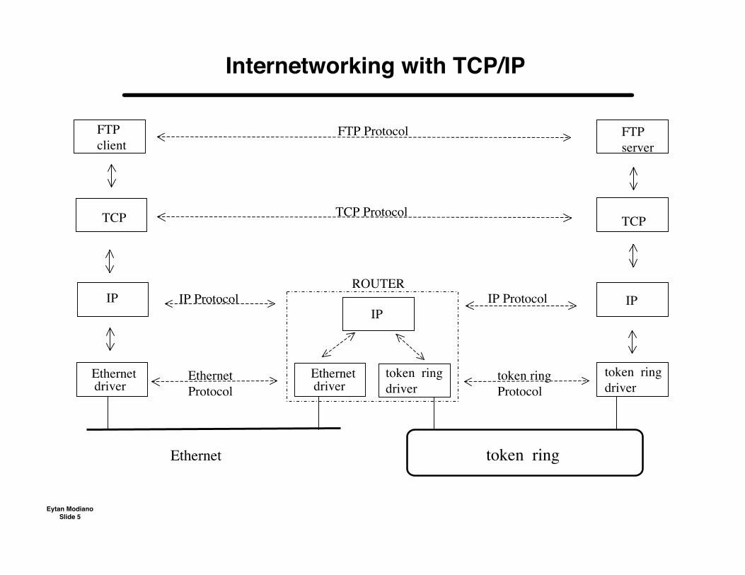
Internetworking with TCP/IP
FTP client
FTPserver
FTP Protocol
TCP TCP Protocol
IP IP Protocol IP Protocol
Ethernet Ethernet Protocol
token ring driver
token ringProtocol
Ethernet
driver
TCP
IPROUTER
IP
Ethernetdriver
token ring driver
token ring

Eytan ModianoSlide 6
Encapsulation
Ethernet
Ethernet
Application
user data
Appluser dataheader
TCPheader application data
headerIP TCP
header application data
IP datagram
TCPheader application dataheader
IPEthernetheader
Ethernettrailer
Ethernet frame
46 to 1500 bytes
14 420 20
driver
IP
TCP
TCP segment

Eytan ModianoSlide 7
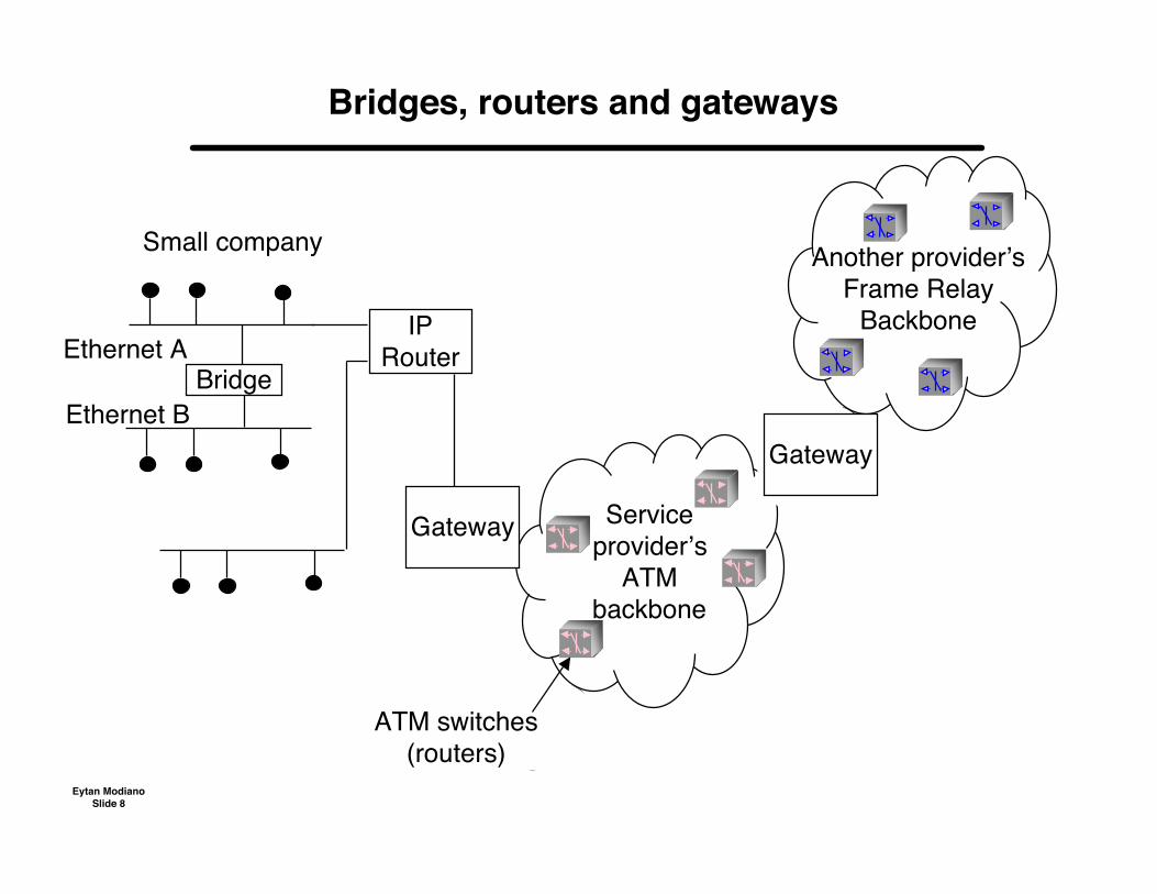
Bridges, Routers and Gateways
• A Bridge is used to connect multiple LAN segments– Layer 2 routing (Ethernet)– Does not know IP address– Varying levels of sophistication
Simple bridges just forward packets smart bridges start looking like routers
• A Router is used to route connect between different networksusing network layer address
– Within or between Autonomous Systems– Using same protocol (e.g., IP, ATM)
• A Gateway connects between networks using different protocols– Protocol conversion– Address resolution
• These definitions are often mixed and seem to evolve!
Eytan ModianoSlide 8
Ethernet A
Ethernet BBridge
IPRouter
Small company
Gateway Serviceprovider’s
ATMbackbone
ATM switches(routers)
Gateway
Another provider’sFrame Relay
Backbone
Bridges, routers and gateways

Eytan ModianoSlide 9
IP addresses
• 32 bit address written as four decimal numbers– One per byte of address (e.g., 155.34.60.112)
• Hierarchical address structure– Network ID/ Host ID/ Port ID– Complete address called a socket– Network and host ID carried in IP Header– Port ID (sending process) carried in TCP header
• IP Address classes:
Net ID Host ID
Net ID
Net ID
Host ID
Host ID
0
10
110
8 32
16 32
24 32
Class A Nets
Class B Nets
Class C Nets
Class D is for multicast traffic

Eytan ModianoSlide 10
Host Names
• Each machine also has a unique name
• Domain name System: A distributed database that provides amapping between IP addresses and Host names
• E.g., 155.34.50.112 => plymouth.ll.mit.edu

Eytan ModianoSlide 11
Internet Standards
• Internet Engineering Task Force (IETF)– Development on near term internet standards– Open body– Meets 3 times a year
• Request for Comments (RFCs)– Official internet standards– Available from IETF web page: http://www.ietf.org

Eytan ModianoSlide 12
The Internet Protocol (IP)
• Routing of packet across the network• Unreliable service
– Best effort delivery– Recovery from lost packets must be done at higher layers
• Connectionless– Packets are delivered (routed) independently– Can be delivered out of order– Re-sequencing must be done at higher layers
• Current version V4
• Future V6– Add more addresses (40 byte header!)– Ability to provide QoS

Eytan ModianoSlide 13
Header Fields in IP
Note that the minimum size header is 20 bytes; TCP
also has 20 byte header

Eytan ModianoSlide 14
IP HEADER FIELDS
• Vers: Version # of IP (current version is 4)• HL: Header Length in 32-bit words• Service: Mostly Ignored• Total length Length of IP datagram• ID Unique datagram ID• Flags: NoFrag, More• FragOffset: Fragment offset in units of 8 Octets• TTL: Time to Live in "seconds” or Hops• Protocol: Higher Layer Protocol ID #• HDR Cksum: 16 bit 1's complement checksum (on header only!)• SA & DA: Network Addresses
• Options: Record Route,Source Route,TimeStamp

Eytan ModianoSlide 15
FRAGMENTATION
• A gateway fragments a datagram if length is too great for nextnetwork (fragmentation required because of unknown paths).
• Each fragment needs a unique identifier for datagram plusidentifier for position within datagram
• In IP, the datagram ID is a 16 bit field counting datagram fromgiven host
ethernet
mtu=1500
X.25
G
GMTU = 512
ethernet
mtu=1500
Eytan ModianoSlide 16
POSITION OF FRAGMENT
• Fragment offset field gives starting position of fragment withindatagram in 8 byte increments (13 bit field)
• Length field in header gives the total length in bytes (16 bit field)
– Maximum size of IP packet 64K bytes
• A flag bit denotes last fragment in datagram
• IP reassembles fragments at destination and throws them away ifone or more is too late in arriving
Eytan ModianoSlide 17
IP Routing
• Routing table at each node contains for each destination the nexthop router to which the packet should be sent
– Not all destination addresses are in the routing table Look for net ID of the destination “Prefix match” Use default router
• Routers do not compute the complete route to the destination butonly the next hop router
• IP uses distributed routing algorithms: RIP, OSPF• In a LAN, the “host” computer sends the packet to the default
router which provides a gateway to the outside world

Eytan ModianoSlide 18
Subnet addressing
• Class A and B addresses allocate too many hosts to a given net• Subnet addressing allows us to divide the host ID space into
smaller “sub networks”– Simplify routing within an organization– Smaller routing tables– Potentially allows the allocation of the same class B address to more
than one organization• 32 bit Subnet “Mask” is used to divide the host ID field into
subnets– “1” denotes a network address field– “0” denotes a host ID field
Class BAddress
16 bit net ID 16 bit host ID
140.252 Subnet ID Host ID
Mask 111111 111 1111111 11111111 00000000
Eytan ModianoSlide 19
Classless inter-domain routing (CIDR)
• Class A and B addresses allocate too many hosts to anorganization while class C addresses don’t allocate enough
– This leads to inefficient assignment of address space• Classless routing allows the allocation of addresses outside of
class boundaries (within the class C pool of addresses)– Allocate a block of contiguous addresses
E.g., 192.4.16.1 - 192.4.32.155 Bundles 16 class C addresses The first 20 bits of the address field are the same and are essentially the
network ID– Network numbers must now be described using their length and
value (I.e., length of network prefix)– Routing table lookup using longest prefix match
• Notice similarity to subnetting - “supernetting”
Eytan ModianoSlide 20
Dynamic Host Configuration (DHCP)
• Automated method for assigning network numbers– IP addresses, default routers
• Computers contact DHCP server at Boot-up time• Server assigns IP address• Allows sharing of address space
– More efficient use of address space– Adds scalability
• Addresses are “least” for some time– Not permanently assigned

Eytan ModianoSlide 21
Address Resolution Protocol
• IP addresses only make sense within IP suite• Local area networks, such as Ethernet, have their own addressing
scheme– To talk to a node on LAN one must have its physical address
(physical interface cards don’t recognize their IP addresses)• ARP provides a mapping between IP addresses and LAN
addresses• RARP provides mapping from LAN addresses to IP addresses• This is accomplished by sending a “broadcast” packet requesting
the owner of the IP address to respond with their physical address– All nodes on the LAN recognize the broadcast message– The owner of the IP address responds with its physical address
• An ARP cache is maintained at each node with recent mappings
IP
EthernetARP RARP

Eytan ModianoSlide 22
Routing in the Internet
• The internet is divided into sub-networks, each under the controlof a single authority known as an Autonomous System (AS)
• Routing algorithms are divided into two categories:– Interior protocols (within an AS)– Exterior protocols (between AS’s)
• Interior Protocols use shortest path algorithms (more later)– Distance vector protocols based on Bellman-ford algorithm
Nodes exchange routing tables with each other E.g., Routing Information Protocol (RIP)
– Link state protocols based on Dijkstra’s algorithm Nodes monitor the state of their links (e.g., delay) Nodes broadcast this information to all of the network E.g., Open Shortest Path First (OSPF)
• Exterior protocols route packets across AS’s– Issues: no single cost metric, policy routing, etc..– Routes often are pre-computed– Example protocols: Exterior Gateway protocol (EGP) and Border
Gateway protocol (BGP)

Eytan ModianoSlide 23
IPv6
• Effort started in 1991 as IPng• Motivation
– Need to increase IP address space– Support for real time application - “QoS”– Security, Mobility, Auto-configuration
• Major changes– Increased address space (16 bytes)
1500 IP addresses per sq. ft. of earth! Address partition similar to CIDR
– Support for QoS via Flow Label field– Simplified header
• Most of the reasons for IPv6 have been taken careof in IPv4
– Is IPv6 really needed?– Complex transition from V4 to V6
0 31ver class Flow labellength Hop limitnexthd
Source address
Destination address

Eytan ModianoSlide 24
Resource Reservation (RSVP)
• Service classes (defined by IETF)– Best effort– Guaranteed service
Max packet delay– Controlled load
emulate lightly loaded network via priority queueing mechanism• Need to reserve resources at routers along the path• RSVP mechanism
– Packet classification Associate packets with sessions (use flow field in IPv6)
– Receiver initiated reservations to support multicast– “soft state” - temporary reservation that expires after 30 seconds
Simplify the management of connections Requires refresh messages
– Packet scheduling to guarantee service Proprietary mechanisms (e.g., Weighted fair queueing)
• Scalability Issues– Each router needs to keep track of large number of flows that grows
with the size (capacity) of the router
Eytan ModianoSlide 25
Differentiated Services (Diffserv)
• Unlike RSVP Diffserv does not need to keep track of individualflows
– Allocate resources to a small number of classes of traffic Queue packets of the same class together
– E.g., two classes of traffic - premium and regular Use one bit to differential between premium and regular packets
– Issues Who sets the premium bit? How is premium service different from regular?
• IETF propose to use TOS field in IP header to identify traffic classes
– Potentially more than just two classes
Eytan ModianoSlide 26
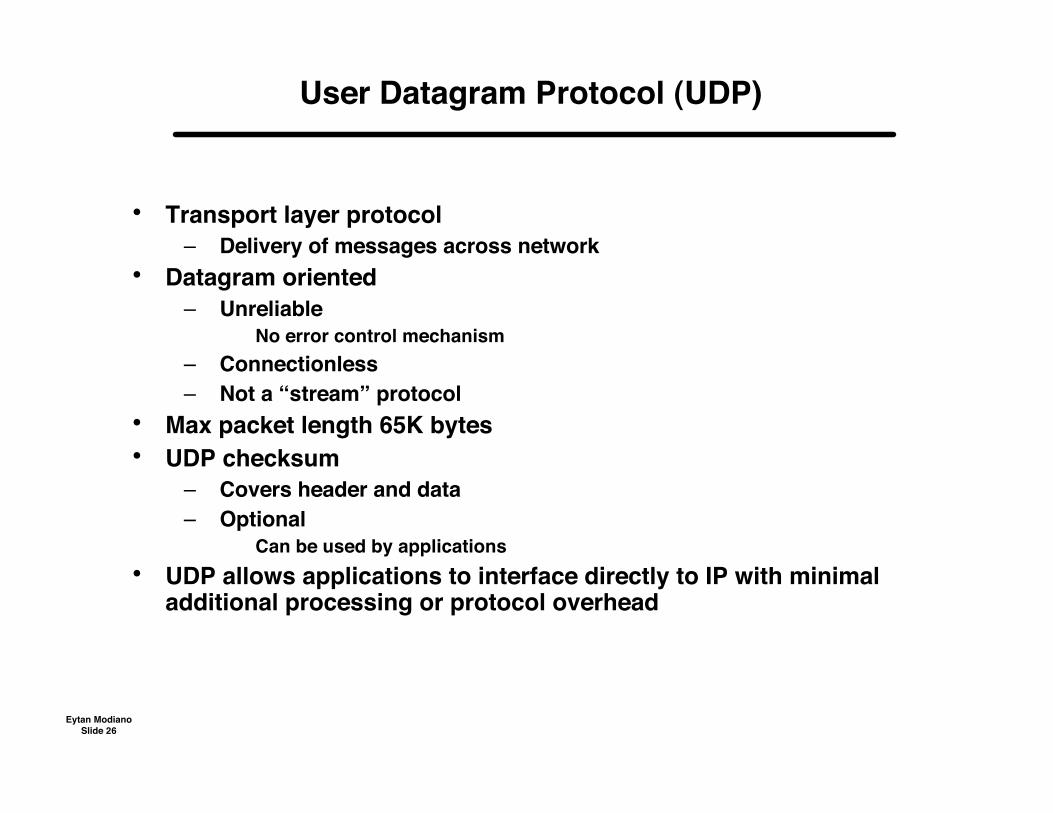
User Datagram Protocol (UDP)
• Transport layer protocol– Delivery of messages across network
• Datagram oriented– Unreliable
No error control mechanism– Connectionless– Not a “stream” protocol
• Max packet length 65K bytes• UDP checksum
– Covers header and data– Optional
Can be used by applications• UDP allows applications to interface directly to IP with minimal
additional processing or protocol overhead

Eytan ModianoSlide 27
UDP header format
• The port numbers identifie the sending and receiving processes– I.e., FTP, email, etc..– Allow UDP to multiplex the data onto a single stream
• UDP length = length of packet in bytes– Minimum of 8 and maximum of 2^16 - 1 = 65,535 bytes
• Checksum covers header and data– Optional, UDP does not do anything with the checksum
IP Datagram
IP header UDP header data
16 bit source port number 16 bit destination port number16 bit UDP length 16 bit checksum
Data

Eytan ModianoSlide 28
Transmission Control Protocol (TCP)
• Transport layer protocol– Reliable transmission of messages
• Connection oriented– Stream traffic– Must re-sequence out of order IP packets
• Reliable– ARQ mechanism– Notice that packets have a sequence number and an ack number– Notice that packet header has a window size (for Go Back N)
• Flow control mechanism– Slow start
Limits the size of the window in response to congestion

Eytan ModianoSlide 29
Basic TCP operation
• At sender– Application data is broken into TCP segments– TCP uses a timer while waiting for an ACK of every packet– Un-ACK’d packets are retransmitted
• At receiver– Errors are detected using a checksum– Correctly received data is acknowledged– Segments are reassembled into their proper order– Duplicate segments are discarded
• Window based retransmission and flow control

Eytan ModianoSlide 30
TCP header fields
Source port Destination port
Request number
DataOffset Reserved Control Window
Check sum Urgent pointer
Options (if any)
Data
Sequence number
16 32

Eytan ModianoSlide 31
TCP header fields
• Ports number are the same as for UDP• 32 bit SN uniquely identify the application data contained in the
TCP segment– SN is in bytes!– It identify the first byte of data
• 32 bit RN is used for piggybacking ACK’s– RN indicates the next byte that the received is expecting– Implicit ACK for all of the bytes up to that point
• Data offset is a header length in 32 bit words (minimum 20 bytes)• Window size
– Used for error recovery (ARQ) and as a flow control mechanism Sender cannot have more than a window of packets in the network
simultaneously– Specified in bytes
Window scaling used to increase the window size in high speed networks• Checksum covers the header and data

Eytan ModianoSlide 32
TCP error recovery
• Error recovery is done at multiple layers– Link, transport, application
• Transport layer error recovery is needed because– Packet losses can occur at network layer
E.g., buffer overflow– Some link layers may not be reliable
• SN and RN are used for error recovery in a similar way to Go BackN at the link layer
– Large SN needed for re-sequencing out of order packets• TCP uses a timeout mechanism for packet retransmission
– Timeout calculation– Fast retransmission

Eytan ModianoSlide 33
TCP timeout calculation
• Based on round trip time measurement (RTT)– Weighted average
RTT_AVE = a*(RTT_measured) + (1-a)*RTT_AVE
• Timeout is a multiple of RTT_AVE (usually two)– Short Timeout would lead to too many retransmissions– Long Timeout would lead to large delays and inefficiency
• In order to make Timeout be more tolerant of delay variations ithas been proposed (Jacobson) to set the timeout value based onthe standard deviation of RTT
Timeout = RTT_AVE + 4*RTT_SD
• In many TCP implementations the minimum value of Timeout is500 ms due to the clock granularity

Eytan ModianoSlide 34
Fast Retransmit
• When TCP receives a packet with a SN that is greater than theexpected SN, it sends an ACK packet with a request number of theexpected packet SN
– This could be due to out-of-order delivery or packet loss• If a packet is lost then duplicate RNs will be sent by TCP until the
packet it correctly received– But the packet will not be retransmitted until a Timeout occurs– This leads to added delay and inefficiency
• Fast retransmit assumes that if 3 duplicate RNs are received bythe sending module that the packet was lost
– After 3 duplicate RNs are received the packet is retransmitted– After retransmission, continue to send new data
• Fast retransmit allows TCP retransmission to behave more likeSelective repeat ARQ
– Future option for selective ACKs (SACK)

Eytan ModianoSlide 35
TCP congestion control
• TCP uses its window size to perform end-to-end congestioncontrol
– More on window flow control later• Basic idea
– With window based ARQ the number of packets in the networkcannot exceed the window size (CW)
Last_byte_sent (SN) - last_byte_ACK’d (RN) <= CW
• Transmission rate when using window flow control is equal to onewindow of packets every round trip time
R = CW/RTT
• By controlling the window size TCP effectively controls the rate

Eytan ModianoSlide 36
Effect Of Window Size
• The window size is the number of bytes that are allowed to be intransport simultaneously
• Too small a window prevents continuous transmission
• To allow continuous transmission window size must exceed round-tripdelay time
WINDOW WINDOW
WASTED BW

Eytan ModianoSlide 37
Length of a bit (traveling at 2/3C)
At 300 bps 1 bit = 415 miles 3000 miles = 7 bits
At 3.3 kbps 1 bit = 38 miles 3000 miles = 79 bits
At 56 kbps 1 bit = 2 miles 3000 miles = 1.5 kbits
At 1.5 Mbps 1 bit = 438 ft. 3000 miles = 36 kbits
At 150 Mbps 1 bit = 4.4 ft. 3000 miles = 3.6 Mbits
At 1 Gbps 1 bit = 8 inches 3000 miles = 240 Mbits

Eytan ModianoSlide 38
Dynamic adjustment of window size
• TCP starts with CW = 1 packet and increases the window sizeslowly as ACK’s are received
– Slow start phase– Congestion avoidance phase
• Slow start phase– During slow start TCP increases the window by one packet for every
ACK that is received– When CW = Threshold TCP goes to Congestion avoidance phase– Notice: during slow start CW doubles every round trip time
Exponential increase!
• Congestion avoidance phase– During congestion avoidance TCP increases the window by one
packet for every window of ACKs that it receives– Notice that during congestion avoidance CW increases by 1 every
round trip time - Linear increase!
• TCP continues to increase CW until congestion occurs

Eytan ModianoSlide 39
Reaction to congestion
• Many variations: Tahoe, Reno, Vegas• Basic idea: when congestion occurs decrease the window size• There are two congestion indication mechanisms
– Duplicate ACKs - could be due to temporary congestion– Timeout - more likely due to significant congstion
• TCP Reno - most common implementation
– If Timeout occurs, CW = 1 and go back to slow start phase
– If duplicate ACKs occur CW = CW/2 stay in congestion avoidancephase

Eytan ModianoSlide 40
Understanding TCP dynamics
• Slow start phase is actually fast• TCP spends most of its time in Congestion avoidance phase• While in Congestion avoidance
– CW increases by 1 every RTT– CW decreases by a factor of two with every loss
“Additive Increase / Multiplicative decrease”

Eytan ModianoSlide 41
Random Early Detection (RED)
• Instead of dropping packet on queue overflow, drop them probabilistically earlier
• Motivation– Dropped packets are used as a mechanism to force the source to slow down
If we wait for buffer overflow it is in fact too late and we may have to drop many packets Leads to TCP synchronization problem where all sources slow down simultaneously
– RED provides an early indication of congestion Randomization reduces the TCP synchronization problem
• Mechanism– Use weighted average queue size
If AVE_Q > Tmin drop with prob. P If AVE_Q > Tmax drop with prob. 1
– RED can be used with explicit congestionnotification rather than packet dropping
– RED has a fairness property Large flows more likely to be dropped
– Threshold and drop probability valuesare an area of active research
Tmin Tmax
Ave queue length
1
Pmax

Eytan ModianoSlide 42
TCP Error Control
EFFICIENCY VS. BER
CHANNEL BER
EF
FIC
IEN
CY
0
0.1
0.2
0.3
0.4
0.5
0.6
0.7
0.8
0.9
1
1E-07 1E-06 1E-05 1E-04 1E-03 1E-02
S R P1 SEC R/T DELAY
T-1 RATE
1000 BIT PACKETSGO BACK N
WITH TCP
WINDOW CONSTRAINT
• Original TCP designed for low BER, low delay links• Future versions (RFC 1323) will allow for larger windows and selective
retransmissions

Eytan ModianoSlide 43
Impact of transmission errors onTCP congestion control
• TCP assumes dropped packets are due to congestion and respondsby reducing the transmission rate
• Over a high BER link dropped packets are more likely to be due toerrors than to congestion
• TCP extensions (RFC 1323)– Fast retransmit mechanism, fast recovery, window scaling
EFFICIENCY VS BER FOR TCP'S
CONGESTION CONTROL
B E R
EF
FIC
IEN
CY
0
0.1
0.2
0.3
0.4
0.5
0.6
0.7
0.8
0.9
1
1.00E-07 1.00E-06 1.00E-05 1.00E-04 1.00E-03
1,544 KBPS 64 KBPS16 KBPS
2.4 KBPS

Eytan ModianoSlide 44
TCP releases
• TCP standards are published as RFC’s• TCP implementations sometimes differ from one another
– May not implement the latest extensions, bugs, etc.• The de facto standard implementation is BSD
– Computer system Research group at UC-Berkeley– Most implementations of TCP are based on the BSD implementations
SUN, MS, etc.• BSD releases
– 4.2BSD - 1983 First widely available release
– 4.3BSD Tahoe - 1988 Slow start and congestion avoidance
– 4.3BSD Reno - 1990 Header compression
– 4.4BSD - 1993 Multicast support, RFC 1323 for high performance
Eytan ModianoSlide 45
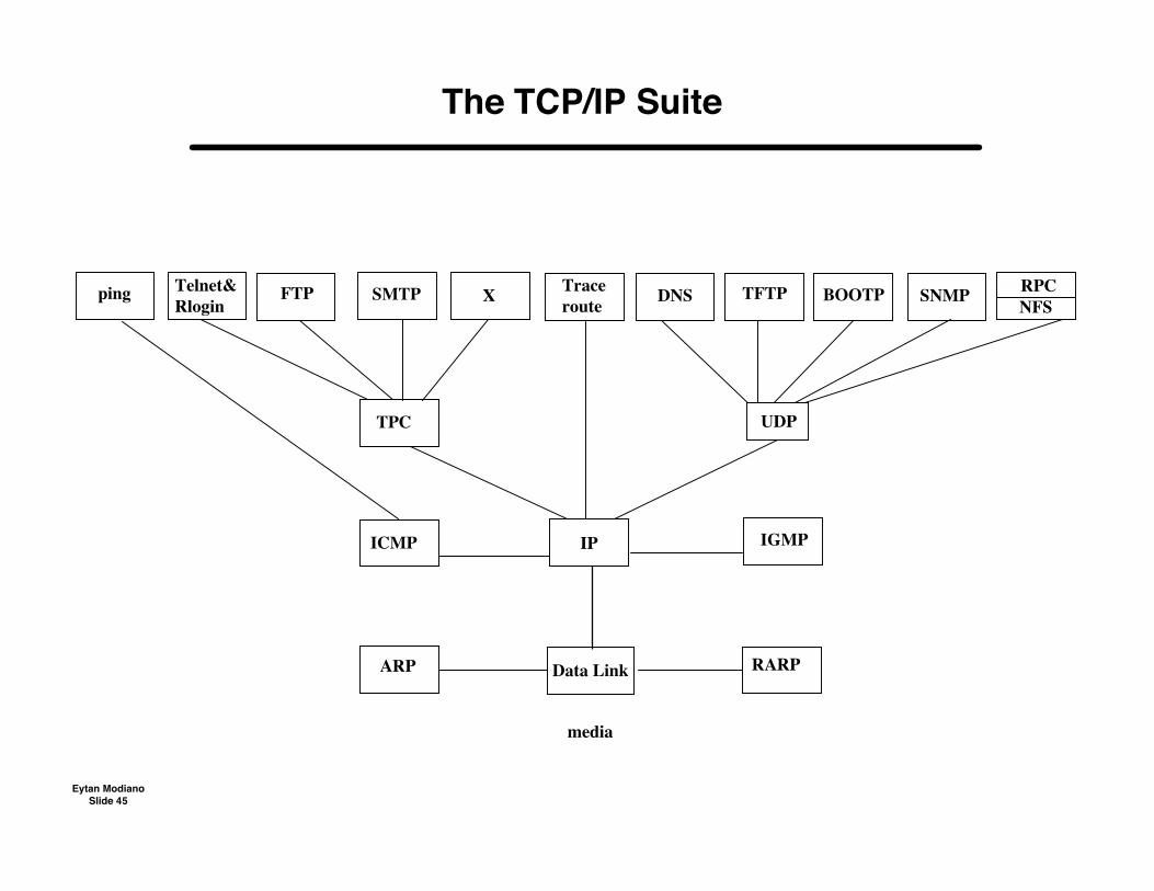
The TCP/IP Suite
UDP
Telnet& Rlogin
FTP SMTP X Traceroute
ping DNS TFTP BOOTP SNMP NFS
TPC
ICMP
ARP
IP
Data Link RARP
IGMP
media
RPC

Eytan ModianoSlide 46
Asynchronous Transfer Mode (ATM)
• 1980’s effort by the phone companies to develop an integratednetwork standard (BISDN) that can support voice, data, video, etc.
• ATM uses small (53 Bytes) fixed size packets called “cells”– Why cells?
Cell switching has properties of both packet and circuit switching Easier to implement high speed switches
– Why 53 bytes?– Small cells are good for voice traffic (limit sampling delays)
For 64Kbps voice it takes 6 ms to fill a cell with data
• ATM networks are connection oriented– Virtual circuits

Eytan ModianoSlide 47
ATM Reference Architecture
• Upper layers– Applications– TCP/IP
• ATM adaptation layer– Similar to transport layer– Provides interface between
upper layers and ATM Break messages into cells and
reassemble
• ATM layer– Cell switching– Congestion control
• Physical layer– ATM designed for SONET
Synchronous optical network TDMA transmission scheme with
125 µs frames
Upper Layers
AT M AdaptationL ayer (AAL )
AT M
Physical

Eytan ModianoSlide 48
ATM Cell format
• Virtual circuit numbers(notice relatively small addressspace!)
– Virtual channel ID– Virtual path ID
• PTI - payload type• CLP - cell loss priority (1 bit!)
– Mark cells that can be dropped• HEC - CRC on header
HEC
PTI
1
2
3
4
5
VPI
CLP
VCI
VPI VCI
VCI
ATM Header (NNI)
Header Data
5 Bytes 48 Bytes
ATM Cell

Eytan ModianoSlide 49
VPI/VCI
• VPI identifies a physical path between the source and destination• VCI identifies a logical connection (session) within that path
– Approach allows for smaller routing tablesand simplifies route computation
ATM Backbone
Use VPI for switching in backbone
Private network
Private network
Private network
Use VCI to ID connectionWithin private network

Eytan ModianoSlide 50
ATM HEADER CRC
• ATM uses an 8 bit CRC that is able to correct 1 error• It checks only on the header of the cell, and alternates between
two modes– In detection mode it does not correct any errors but is able to detect
more errors– In correction mode it can correct up to one error reliably but is less
able to detect errors• When the channel is relatively good it makes sense to be in
correction mode, however when the channel is bad you want to bein detection mode to maximize the detection capability
Correcterrors
Detecterrors
No detectederrors
Correct singleerror
Detect double error
No detected errorsDetectederrors

Eytan ModianoSlide 51
ATM Service Categories
• Constant Bit Rate (CBR) - e.g. uncompressed voice– Circuit emulation
• Variable Bit Rate (rt-VBR) - e.g. compressed video– Real-time and non-real-time
• Available Bit Rate (ABR) - e.g. LAN interconnect– For bursty traffic with limited BW guarantees and congestion control
• Unspecified Bit Rate (UBR) - e.g. Internet– ABR without BW guarantees and congestion control

Eytan ModianoSlide 52
ATM service parameters(examples)
• Peak cell rate (PCR)• Sustained cell rate (SCR)• Maximum Burst Size (MBS)• Minimum cell rate (MCR)• Cell loss rate (CLR)• Cell transmission delay (CTD)• Cell delay variation (CDV)
• Not all parameters apply to all service categories– E.g., CBR specifies PCR and CDV– VBR specifies MBR and SCR
• Network guarantees QoS provided that the user conforms to hiscontract as specified by above parameters
– When users exceed their rate network can drop those packets– Cell rate can be controlled using rate control scheme (leaky bucket)

Eytan ModianoSlide 53
Flow control in ATM networks (ABR)
• ATM uses resource management cells to control rate parameters– Forward resource management (FRM)– Backward resource management (BRM)
• RM cells contain– Congestion indicator (CI)– No increase Indicator (NI)– Explicit cell rate (ER)– Current cell rate (CCR)– Min cell rate (MCR)
• Source generates RM cells regularly– As RM cells pass through the networked they can be marked with
CI=1 to indicate congestion– RM cells are returned back to the source where
CI = 1 => decrease rate by some fraction CI = 1 => Increase rate by some fraction
– ER can be used to set explicit rate

Eytan ModianoSlide 54
End-to-End RM-Cell Flow
At the destination the RM cell is “turned around” and sent back to the source
ABR
Source
ABR
Switch
ABR
Switch
= data cell
= forward RM cell
= backward RM cell
ABR
Destin-
ation
BRM
FRM
D
BRM
D D D FRM D
BRM
D FRM

Eytan ModianoSlide 55
ATM Adaptation Layers
• Interface between ATM layer and higher layer packets• Four adaptation layers that closely correspond
to ATM’s service classes– AAL-1 to support CBR traffic– AAL-2 to support VBR traffic– AAL-3/4 to support bursty data traffic– AAL-5 to support IP with minimal overhead
• The functions and format of the adaptation layer depend on theclass of service.
– For example, stream type traffic requires sequence numbers toidentify which cells have been dropped.
USER PDU (DLC or NL)
ATM CELL
ATM CELL
Each class of service hasA different header format(in addition to the 5 byte ATM header)

Eytan ModianoSlide 56
Example: AAL 3/4
• ST: Segment Type (1st, Middle, Last)• SEQ:4-bit sequence number (detect lost cells)• MID: Message ID (reassembly of multiple msgs)• 44 Byte user payload (~84% efficient)• LEN: Length of data in this segment• CRC: 10 bit segment CRC
• AAL 3/4 allows multiplexing, reliability, & error detection but isfairly complex to process and adds much overhead
• AAL 5 was introduced to support IP traffic– Fewer functions but much less overhead and complexity
ATM CELL PAYLOAD (48 Bytes)
LEN CRC
6 10
ST SEQ MID
2 4 10
44 Byte User Payload

Eytan ModianoSlide 57
ATM cell switches
Input
Q's
Output
Q's
S/WControl
InputCell
Processing
InputCell
Processing
InputCell
Processing
Output
Output
Output
Switch
Fabric
11
22
m m
• Design issues– Input vs. output queueing– Head of line blocking– Fabric speed

Eytan ModianoSlide 58
ATM summary
• ATM is mostly used as a “core” network technology
• ATM Advantages
– Ability to provide QoS– Ability to do traffic management– Fast cell switching using relatively short VC numbers
• ATM disadvantages– It not IP - most everything was design for TCP/IP– It’s not naturally an end-to-end protocol
Does not work well in heterogeneous environment Was not design to inter-operate with other protocols Not a good match for certain physical media (e.g., wireless)
– Many of the benefits of ATM can be “borrowed” by IP Cell switching core routers Label switching mechanisms
Eytan ModianoSlide 59
Multi-Protocol Label Switching (MPLS)
“As more services with fixed throughput anddelay requirements become more common, IPwill need virtual circuits (although it will probablycall them something else)”
Data Networks lecture notes - April 28, 1994

Eytan ModianoSlide 60
Label Switching
• Router makers realize that in order to increase the speed andcapacity they need to adopt a mechanism similar to ATM
– Switch based on a simple tag not requiring complex routing tablelook-ups
– Use virtual circuits to manage the traffic (QoS)– Use cell switching at the core of the router
• First attempt: IP-switching– Routers attempt to identify flows
Define a flow based on observing a number of packets between a givensource and destination (e.g., 5 packets within a second)
– Map IP source-destination pairs to ATM VC’s Distributed algorithm where each router makes its own decision
• Multi-protocol label switching (MPLS)– Also known as Tag switching– Does not depend on ATM– Add a tag to each packet to serve as a VC number
Tags can be assigned permanently to certain paths

Eytan ModianoSlide 61
Label switching can be used to create a virtualmesh with the core network
• Routers at the edge of the corenetwork can be connected toeach other using labels
• Packets arriving at an edge routercan be tagged with the label tothe destination edge router
– “Tunneling”
– Significantly simplifies routingin the core
– Interior routers need notremember all IP prefixes ofoutside world
– Allows for traffic engineering Assign capacity to labels based
on demand
Core network
Label switched routes
D
D

Eytan ModianoSlide 62
References
• TCP/IP Illustrated (Vols. 1&2), Stevens
• Computer Networks, Peterson and Davie
• High performance communication networks, Walrand and Varaiya
Recommended