Documents de Travail du Centre d’Economie de la Sorbonne
On the existence of a Ramsey equilibrium with endogenous
labor supply and borrowing constraints
Stefano BOSI, Cuong LE VAN
2011.45
Maison des Sciences Économiques, 106-112 boulevard de L'Hôpital, 75647 Paris Cedex 13 http://centredeconomiesorbonne.univ-paris1.fr/bandeau-haut/documents-de-travail/
ISSN : 1955-611X
hals
hs-0
0612
131,
ver
sion
1 -
28 J
ul 2
011
On the existence of a Ramsey equilibrium
with endogenous labor supply
and borrowing constraints∗
Stefano Bosi†and Cuong Le Van‡
July 22, 2011
∗We would like to thank Thomas Seegmuller for comments that have significantly improvedthe paper, and Robert Becker. This model has been presented to the international conference
New Challenges for Macroeconomic Regulation held on June 2011 in Marseille.†THEMA. E-mail: [email protected].‡CNRS, CES, Exeter University, Paris School of Economics, VCREME. E-mail:
1
Documents de Travail du Centre d'Economie de la Sorbonne - 2011.45
hals
hs-0
0612
131,
ver
sion
1 -
28 J
ul 2
011
Résumé
Dans ce papier, on étudie l’existence d’un équilibre intertemporel dans un
modèle de Ramsey avec escompte hétérogène, offre de travail élastique et con-
traintes d’emprunt. En appliquant un argument de point fixe de Gale et Mas-
Colell (1975), on démontre l’existence d’un équilibre dans une économie bornée
tronquée. Cet équilibre est aussi un équilibre pour toute économie non bornée
aux mêmes fondamentaux. Enfin, on montre l’existence d’un équilibre dans
une économie à horizon infini comme limite d’une suite d’économies tronquées.
D’une part, notre papier généralise Becker et al. (1991) à cause de l’offre de
travail élastique et, d’autre part, Bosi et Seegmuller (2010) à cause d’une dé-
monstration d’existence globale. Notre méthodologie peut aussi s’appliquer à
d’autres modèles de Ramsey avec des imperfections de marché différentes.
Mots-clés : Existence de l’équilibre ; Modèle de Ramsey ; Agents hétérogènes
; Offre de travail endogène ; Contraintes d’emprunt
Classification JEL : C62, D31, D91
Abstract
In this paper, we study the existence of an intertemporal equilibrium in
a Ramsey model with heterogenous discounting, elastic labor supply and bor-
rowing constraints. Applying a fixed-point argument by Gale and Mas-Colell
(1975), we prove the existence of an equilibrium in a truncated bounded econ-
omy. This equilibrium is also an equilibrium of any unbounded economy with
the same fundamentals. Finally, we prove the existence of an equilibrium in an
infinite-horizon economy as a limit of a sequence of truncated economies. On
the one hand, our paper generalizes Becker et al. (1991) because of the elastic
labor supply and, on the other hand, Bosi and Seegmuller (2010) because of a
proof of global existence. Our methodology can be also applied to other Ramsey
models with different market imperfections.
Keywords: Existence of equilibrium; Ramsey model; Heterogeneous agents;
Endogenous labor supply; Borrowing constraint
JEL classification: C62, D31, D91
2
Documents de Travail du Centre d'Economie de la Sorbonne - 2011.45
hals
hs-0
0612
131,
ver
sion
1 -
28 J
ul 2
011
1 Introduction
Ramsey (1928) remains the most influential paper in growth literature and an
inexhaustible source of inspiration for theorists. One of the puzzling aspects of
the model is the so-called Ramsey conjecture: "... equilibrium would be attained
by a division into two classes, the thrifty enjoying bliss and the improvident at
the subsistence level" (Ramsey (1928), p. 559). This sentence ends the paper
and means that, in the long run, the most patient agents would hold all the
capital, while the others would live at their subsistence level. The Ramsey
conjecture was proved by Robert Becker more than half a century later.
Becker (1980) pioneers a series of works during three decades on the prop-
erties of a Ramsey equilibrium under heterogenous discounting.1 He shows the
existence of a long-run equilibrium where the most patient agent holds the cap-
ital of the economy, while the impatient ones consume their labor income. The
existence of the steady state rests on the introduction of borrowing constraints
that prevent agents to borrow against their future labor income.
The complete markets case is considered by other authors. Le Van and
Vailakis (2003) prove that, when individuals are allowed to borrow against fu-
ture income, the impatient agents borrow from the patient one and spend the
rest of their life to work to refund the debt. In addition, their consumption
asymptotically vanishes and there is no longer room for a steady state. The
extension with elastic labor supply, which is pertinent for a comparison with
our paper, is provided by Le Van et al. (2007).
Borrowing constraints are credit market imperfections that change the equi-
librium properties in terms of: (1) optimality, (2) stationarity and (3) monotonic-
ity.
(1) Optimality. Credit market incompleteness entails the failure of the first
welfare theorem. As a matter of fact, it is no longer possible to prove the
existence of a competitive equilibrium by studying the set of Pareto-efficient
allocations as done by Le Van and Vailakis (2003) and Le Van et al. (2007),
among others, in absence of market imperfections.
(2) Stationarity. Under borrowing constraints, there exists a stationary state
where impatient agents consume. The steady state vanishes when these con-
straints are retired: in the complete markets counterpart, Le Van and Vailakis
(2003) and Le Van et al. (2007) show that the convergence of the optimal capi-
tal sequence to a particular stock still holds, but this stock is not itself a steady
state.
(3) Monotonicity. In presence of borrowing constraints, persistent cycles
arise (Becker (1980), Becker and Foias (1987, 1994), Sorger (1994)). To un-
derstand the role of these constraints, it is worthy to compare with similar
models where markets are complete: Le Van and Vailakis (2003) and Le Van
et al. (2007) also find that, under discounting heterogeneity, the monotonicity
property of the representative agent counterpart does not carry over and that
a twisted turnpike property holds (see Mitra (1979) and Becker (2005)). The
1For a survey on this literature, the reader is referred to Becker (2006).
3
Documents de Travail du Centre d'Economie de la Sorbonne - 2011.45
hals
hs-0
0612
131,
ver
sion
1 -
28 J
ul 2
011
very difference with the class of models à la Becker is that the optimal capi-
tal sequence always converges in the long run and, thus, there is no room for
persistent cycles.
What is the reason of persistence? Becker and Foias (1987, 1994) show that
cycles of period two may occur when capital income monotonicity fails, that is
capital income is decreasing in the capital stock.
Thereby, the Ramsey conjecture holds under perfect competition, but also
under the kind of imperfection represented by financial constraints. However,
the introduction of other forms of imperfections makes this conjecture frag-
ile. Prominent examples are given by distortionary taxation and market power.
Sarte (1997) and Sorger (2002) study a progressive capital income taxation,
while Sorger (2002, 2005, 2008) and Becker and Foias (2007) focus on the strate-
gic interaction in the capital market. They prove the possibility of a long-run
non-degenerated distribution of capital where impatient agents hold capital.
Our paper addresses the difficult question of the existence of an intertempo-
ral equilibrium under borrowing constraints. The usual proof of existence à la
Negishi no longer applies because markets are imperfect.
Becker et al. (1991) have shown the existence of an intertemporal equilibrium
under borrowing constraints with inelastic labor supply. The argument of the
proof rests on the introduction of a tâtonnement map giving an equilibrium as
a fixed point of the map.
Bosi and Seegmuller (2010) provide a local proof of existence of an intertem-
poral equilibrium with elastic labor supply. Their argument rests on the exis-
tence of a local fixed point for the policy function based on the local stability
properties of the steady state.
In this respect, the novelty of our paper is twofold.
(1) We generalize Becker et al. (1991) by considering an elastic labor supply.
(2) We go beyond Bosi and Seegmuller (2010) by providing a proof of global
existence.
We show the existence of an intertemporal equilibrium in presence of market
imperfections by applying a method inspired by Florenzano (1999), a model with
incomplete markets. This method is based on a Gale and Mas-Colell (1975)
fixed-point argument and can be applied in other contexts.
The entire paper is devoted to the proof of existence and is articulated in
two steps.
(1) We first consider a time-truncated economy. Since the feasible alloca-
tions sets of our economy are uniformly bounded, we prove that there exists an
equilibrium in a time-truncated bounded economy by using a theorem by Gale
and Mas-Colell (1975). Actually, this equilibrium turns out to be an equilibrium
for the time-truncated economy.
(2) Second, we take the limit of a sequence of truncated unbounded economies
and we prove the existence of an intertemporal equilibrium in the limit economy.
These points correspond to the two main sections of the paper. Most of the
proofs are given in Appendices 1 and 2.
4
Documents de Travail du Centre d'Economie de la Sorbonne - 2011.45
hals
hs-0
0612
131,
ver
sion
1 -
28 J
ul 2
011
2 Firms
We consider a representative firm with no market power. The technology is rep-
resented by a constant returns to scale production function: ( ), where
and are the aggregate capital and the aggregate labor. Profit max-
imization: max [ ( )− − ], gives = and
= . We introduce the set of nonnegative real numbers: R+ ≡{ ∈ R : ≥ 0}. Profit maximization is correctly defined under the followingassumption.2
Assumption 1 : R2+ → R+ is 1, constant returns to scale, strictly increas-ing and concave. We assume that inputs are essential: (0 ) = ( 0) = 0.
In addition, () → +∞ when 0 and → +∞ or when 0 and
→ +∞.
Let us introduce also boundary conditions on capital productivity when the
labor supply is maximal and equal to in order to simplify the proof of equi-
librium existence.
Assumption 2 () (0) and () (+∞) , where ∈(0 1) denotes the rate of capital depreciation.
3 Households
We consider an economy without population growth where households work
and consume. Each household is endowed with 0 units of capital at period
0 and 1 unit of leisure-time per period. Leisure demand of agent at time
is denoted by and the individual labor supply is given by = 1 − .
Individual wealth and consumption demand at time are denoted by and
.
Initial capital endowments are supposed to be positive.
Assumption 3 0 0 for = 1 .
It is known that, in economies with heterogenous discounting and no bor-
rowing constraints, impatient agents borrow, consume more and work less in the
short run, and that they consume less and work more in the long run to refund
the debt to patient agents. In our model, agents are prevented from borrowing:
≥ 0 for = 1 2 and = 1 .
2The shortcut of maximization of an aggregate profit rests on the following argument.
Consider a large number of firms that share the same technology and have no market power.
Each firm maximizes the profit ( ) − − in every period: = 0 1
This gives = and = which in turn implies that the ratio
is the same across the firms. Let ( ) ≡
=1
=1
be the aggregate solution.
We define an aggregate production function: ( ). Since productivities and
are homogeneous of degree zero, the aggregate solution is also solution of the aggregate
program: max [ ( )− −].
5
Documents de Travail du Centre d'Economie de la Sorbonne - 2011.45
hals
hs-0
0612
131,
ver
sion
1 -
28 J
ul 2
011
Each household maximizes a utility separable over time:P
=0 ( ),
where ∈ (0 1) is the discount factor of agent .
Assumption 4 : R2+ → R is 1, strictly increasing and concave.
4 Definition of equilibrium
We define an infinite-horizon sequences of prices and quantities:
(p rw (ckλ)=1 KL)
where
(p rw) ≡ (()∞=0 ()
∞=0 ()
∞=0) ∈ R∞ ×R∞+ ×R∞+
(ckλ) ≡ (()∞=0 ()
∞=1 ()
∞=0) ∈ R∞+ ×R∞ ×R∞+
(KL) ≡ (()∞=0 ()
∞=0) ∈ R∞+ ×R∞+
with = 1 .
Definition 1 A Walrasian equilibrium¡p r w
¡c k λ
¢=1
K L¢satisfies
the following conditions.
(1) Price positivity: 0 for = 0 1
(2) Market clearing:
goods :
X=1
£ + +1 − (1− )
¤=
¡
¢capital : =
X=1
labor : =
X=1
for = 0 1 , where = 1− denotes the individual labor supply.
(3) Optimal production plans: ¡
¢ − − is the value of
the program: max [ ( )− − ], for = 0 1 under the con-
straints ≥ 0 and ≥ 0.(4) Optimal consumption plans:
P∞=0
¡
¢is the value of the pro-
gram: maxP∞
=0 ( ), under the following constraints:
budget constraint : [ + +1 − (1− ) ] ≤ + (1− )
borrowing constraint : +1 ≥ 0leisure endowment : 0 ≤ ≤ 1capital endowment : 0 ≥ 0 given
for = 0 1
6
Documents de Travail du Centre d'Economie de la Sorbonne - 2011.45
hals
hs-0
0612
131,
ver
sion
1 -
28 J
ul 2
011
The following claims are essential in our paper.
Claim 1 Labor supply is bounded.
Proof. At the individual level, because = 1− ∈ [0 1]. At the aggregatelevel, because 0 ≤P
=1 ≤ .
Claim 2 Under Assumptions 1 and 2, individual and aggregate capital supplies
are bounded.
Proof. At the individual level, because of the borrowing constraint, we have
0 ≤ ≤P
=1 .
To prove that the individual capital supply is bounded, we prove that the
aggregate capital supply is bounded. We want to show that 0 ≤ P=1 ≤
max {P=1 0} ≡ , where is the unique solution of
= (1− )+ () (1)
Since is 1, increasing and concave, (0 ) = 0 and
1− + () (0) 1 1− + () (+∞)
(Assumptions 1 and 2), the solution of (1) is unique. Moreover, ≤ implies
(1− ) + () ≤ (2)
We notice that
X=1
+1 ≤X=1
( + +1) ≤ (1− )
X=1
+
ÃX=1
X=1
!
≤ (1− )
X=1
+
ÃX=1
!because is increasing, the capital employed cannot exceed its aggregate supplyP
=1 andP
=1 ≤ . Let ≡P
=1 . Then, +1 ≤ (1− ) +
().
We observe that 0 ≤ max { 0} ≡ . Therefore, 1 ≤ (1− )0 +
(0) ≤ (1− ) + () ≤ because ≤ and, from (2), (1 −)+ () ≤ . Iterating the argument, we find ≤ for = 0 1
Claim 3 Under Assumptions 1 and 2, consumption is bounded.
Proof. At the individual level, we have 0 ≤ ≤P
=1 .
To prove that the individual consumption is bounded, we prove that the
aggregate consumption is bounded.
X=1
≤X=1
( + +1) ≤ (1− )
X=1
+
ÃX=1
!≤ (1− )+ () ≤
7
Documents de Travail du Centre d'Economie de la Sorbonne - 2011.45
hals
hs-0
0612
131,
ver
sion
1 -
28 J
ul 2
011
5 On the existence of equilibrium in a finite-
horizon economy
We consider an economy which goes on for + 1 periods: = 0 .
Focus first on a bounded economy, that is choose sufficiently large bounds
for quantities:
≡ {(0 ) : 0 ≤ ≤ } = [0 ]+1
with
≡ {(1 ) : 0 ≤ ≤ } = [0 ]with
≡ {(0 ) : 0 ≤ ≤ 1} = [0 1]+1
≡ {(0 ) : 0 ≤ ≤ } = [0 ]+1
with
≡ {(0 ) : 0 ≤ ≤ } = [0 ]+1
with
We notice that 0 is given and that the borrowing constraints (inequalities
≥ 0) capture the imperfection in the credit market.3Let E denote this economy with technology and preferences as in Assump-
tions 1 to 4 and with , and as the th consumer-worker’s bounded
sets of consumption demand, capital supply and leisure demand respectively
( = 1 ), and and as the firm’s bounded sets of capital and labor
demands respectively.
Proposition 1 Under the Assumptions 1, 2, 3 and 4, there exists an equilib-
rium ¡p r w
¡c k λ
¢=1
K L¢
for the finite-horizon bounded economy E .Proof. The proof is quite long and articulated in many claims (see Appendix
1).
Focus now on an unbounded economy.
Theorem 4 Any equilibrium of E is an equilibrium for the finite-horizon un-
bounded economy.
Proof. Let¡p r w
¡c k λ
¢=1
K L¢with 0, = 0 , be
an equilibrium of E .Let (ckλ) verify
P=0
( )
P=0
¡
¢. We want to
prove that this allocation violates at least one budget constraint, that is that
there exists such that
[ + +1 − (1− ) ] + (1− ) (3)
Focus on a strictly convex combination of (ckλ) and¡c k λ
¢:
() ≡ + (1− )
() ≡ + (1− ) (4)
() ≡ + (1− )
3A possible generalization of credit constraints is ≤ with 0 given.
8
Documents de Travail du Centre d'Economie de la Sorbonne - 2011.45
hals
hs-0
0612
131,
ver
sion
1 -
28 J
ul 2
011
with 0 1. Notice that we assume that the bounds satisfy
and in order ensure that we enter the bounded economy when the
parameter is sufficiently close to 0.
Entering the bounded economy means (c () k () λ ()) ∈ ××.
In this case, because of the concavity of the utility function, we find
X=0
( () ()) ≥
X=0
( ) + (1− )
X=0
¡
¢
X=0
¡
¢Since (c () k () λ ()) ∈ ×× and
¡p r w
¡c k λ
¢=1
K L¢
is an equilibrium for this economy, there exists ∈ {0 } such that [ () + +1 ()− (1− ) ()] () + (1− ())
Replacing (4), we obtain
¡ + (1− ) + +1 + (1− ) +1 − (1− )
£ + (1− )
¤¢
£ + (1− )
¤+
¡1− £ + (1− )
¤¢that is
[ + +1 − (1− ) ] + (1− ) £ + +1 − (1− )
¤ [ + (1− )] + (1− )
£ +
¡1−
¢¤Since
£ + +1 − (1− )
¤= +
¡1−
¢, we obtain (3). Thus¡
p r w¡c k λ
¢=1
K L¢is also an equilibrium for this unbounded econ-
omy.
6 On the existence of equilibrium in an infinite-
horizon economy
In the section, we introduce a separable utility and, for simplicity, we denote
by the utility of consumption and by that of leisure. If is the utility
defined on both these arguments, we have ( ) ≡ () + ().
Assumption 5 The utility function is separable: ( ) ≡ ()+ (),
with : R+ → R and ∈ 1. In addition, we assume that (0) =
(0) = 0, 0 (0) = 0 (0) = +∞, 0 () 0 () 0 for 0, and that
functions are concave.
Theorem 5 Under the Assumptions 1, 2, 3 and 5, there exists an equilibrium
in the infinite-horizon economy with endogenous labor supply and borrowing
constraints.
9
Documents de Travail du Centre d'Economie de la Sorbonne - 2011.45
hals
hs-0
0612
131,
ver
sion
1 -
28 J
ul 2
011
Proof. We consider a sequence of time-truncated economies and the associated
equilibria. We prove that there exists a sequence of equilibria which converges,
when the horizon goes to infinity, to an equilibrium of the infinite-horizon
economy. The proof is detailed in Appendix 2.
7 Conclusion
In this paper, we have shown the existence of an intertemporal equilibrium with
market imperfections (borrowing constraints). Applying the fixed-point theorem
of Gale-Mas-Colell, we have proved the existence of an equilibrium in a finite-
horizon bounded economy. This equilibrium turns out to be also an equilibrium
of any unbounded economy with the same fundamentals. Eventually, we have
shown the existence of an equilibrium in an infinite-horizon economy as a limit of
a sequence of truncated economies by applying a uniform convergence argument.
The paper generalizes in one respect Becker et al. (1991) by considering
an elastic labor supply, and, in another respect, Bosi and Seegmuller (2010) by
providing a proof of global existence. Our methodology, inspired by Florenzano
(1999) is quite general and can be applied to other Ramsey models with different
market imperfections.
8 Appendix 1: finite horizon
Let us prove Proposition 1.
We define a bounded price set:
≡ {(p rw) : −1 ≤ ≤ 1 0 ≤ ≤ 1 0 ≤ ≤ 1 = 0 }At this stage, we put no restriction on the sign of . We will prove later the
positivity of the good price through an equilibrium argument.
Focus now on the budget constraints:
[ + +1 − (1− ) ] ≤ + (1− )
for = 0 − 1 and [ − (1− ) ] ≤ + (1− ).
In the spirit of Bergstrom (1976), we introduce modified budget sets:
(p rw)
≡
⎧⎪⎪⎨⎪⎪⎩(ckλ) ∈ × × :
[ + +1 − (1− ) ] + (1− ) + ( )
= 0 − 1 [ − (1− ) ] + (1− ) + ( )
⎫⎪⎪⎬⎪⎪⎭ (p rw)
≡
⎧⎪⎪⎨⎪⎪⎩(ckλ) ∈ × × :
[ + +1 − (1− ) ] ≤ + (1− ) + ( )
= 0 − 1 [ − (1− ) ] ≤ + (1− ) + ( )
⎫⎪⎪⎬⎪⎪⎭10
Documents de Travail du Centre d'Economie de la Sorbonne - 2011.45
hals
hs-0
0612
131,
ver
sion
1 -
28 J
ul 2
011
where ( ) ≡ 1−min {1 ||+ + }.Let (p rw) denote the closure of (p rw).
Claim 6 For every (p rw) ∈ , we have (p rw) 6= ∅ and (p rw) =
(p rw).
Proof. Without loss of generality, focus on the modified budget constraints of
the first two periods:
0 [0 + 1 − (1− ) 0] 00 + 0 (1− 0) + (0 0 0) (5)
1 [1 + 2 − (1− ) 1] 11 + 1 (1− 1) + (1 1 1) (6)
We know that −1 ≤ ≤ 1, 0 ≤ ≤ 1, 0 ≤ ≤ 1.(1) Assume that |0|+ 0 + 0 1. Then (0 0 0) 0.
Assume to be large enough to set 0 = (1− ) 0 and choose 0 = 1 (we
stay in ×). Then the inequality (5) becomes 01 00 + (0 0 0)
and it is satisfied if 1 0 is sufficiently close to zero.
Focus now on the second period and two subcases.
(1.1) Assume that |1|+ 1 + 1 1. Then (1 1 1) 0.
If 1 0, choose 1 sufficiently large (assume the upper bound to be
large enough) and the inequality (6) is satisfied.
If 1 ≥ 0, set 1 = 2 = 0 and the inequality (6) becomes −1 (1− ) 1
11 + 1 (1− 1) + (1 1 1) and it is satisfied. Notice that, in this case,
inequality (6) is satisfied also if 2 0 but sufficiently close to zero.
(1.2) Assume that |1|+ 1 + 1 ≥ 1. Then (1 1 1) = 0.
If 1 0, choose 1 sufficiently large (assume the upper bound to be
large enough) and the inequality (6) is satisfied.
If 1 = 0, choose 1 = 0. The inequality (6) becomes 0 11 + 1 and,
since either 1 0 or 1 0, it is satisfied because 1 0 (see point (1)).
If 1 0, set 1 = 2 = 0: the inequality (6) becomes −1 (1− ) 1
11 + 1 (1− 1) and is satisfied because 1 0 (see point (1)) and 1.
Notice that, in this case, inequality (6) is satisfied also if 2 0 but sufficiently
close to zero.
(2) Assume that |0|+ 0 + 0 ≥ 1. Then (0 0 0) = 0.
If 0 0, assume to be large enough to set 0 = (1− ) 0 and choose
1 0. Inequality (5) becomes 01 00 + 0 (1− 0) and it is satisfied.
If 0 = 0, we have either 0 0 or 0 0. Set 0 = 0 1. Inequality
(5) becomes 0 00+0. We can not exclude the case 0 = 0 or 0 = 0, but
Assumption 3 ensures that inequality (5) is verified.
If 0 0, set 0 = 0 and 0 1 (1− ) 0. Inequality (5) becomes
0 [1 − (1− ) 0] 00 + 0 (1− 0) and it is satisfied.
Focus on the second period and two subcases.
(2.1) Assume that |1|+ 1 + 1 1. Then (1 1 1) 0.
The same arguments of point (1.1) apply.
(2.2) Assume that |1|+ 1 + 1 ≥ 1. Then (1 1 1) = 0.
The same arguments of point (1.2) apply (just replace "see point (1)" with
"see point (2)").
11
Documents de Travail du Centre d'Economie de la Sorbonne - 2011.45
hals
hs-0
0612
131,
ver
sion
1 -
28 J
ul 2
011
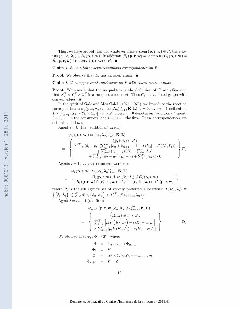
Thus, we have proved that, for whatever price system (p rw) ∈ , there ex-
ists (ckλ) ∈ (p rw). In addition, (p rw) 6= ∅ implies (p rw) =
(p rw) for every (p rw) ∈ .
Claim 7 is a lower semi-continuous correspondence on .
Proof. We observe that has an open graph.
Claim 8 is upper semi-continuous on with closed convex values.
Proof. We remark that the inequalities in the definition of are affine and
that ×
× is a compact convex set. Thus has a closed graph with
convex values.
In the spirit of Gale and Mas-Colell (1975, 1979), we introduce the reaction
correspondences (p rw (ckλ)=1 KL), = 0 + 1 defined on
× [×=1 ( × × )]× ×, where = 0 denotes an "additional" agent,
= 1 the consumers, and = +1 the firm. These correspondences are
defined as follows.
Agent = 0 (the "additional" agent):
0 (p rw (ckλ)=1 KL)
≡
⎧⎪⎪⎨⎪⎪⎩(p r w) ∈ :P
=0 ( − ) (P
=1 [ + +1 − (1− ) ]− ( ))
+P
=0 ( − ) ( −P
=1 )
+P
=0 ( − ) ( −+P
=1 ) 0
⎫⎪⎪⎬⎪⎪⎭ (7)Agents = 1 (consumers-workers):
(p rw (ckλ)=1 KL)
≡½
(p rw) if (ckλ) ∈ (p rw)
(p rw) ∩ [ (cλ)× ] if (ckλ) ∈ (p rw)
¾where is the th agent’s set of strictly preferred allocations: (cλ) ≡n³c λ
´:P
=0
³
´P
=0 ( )
o.
Agent = + 1 (the firm):
+1 (p rw (ckλ)=1 KL)
≡
⎧⎪⎪⎨⎪⎪⎩³K L
´∈ × :P
=0
h
³
´− −
iP
=0 [ ( )− − ]
⎫⎪⎪⎬⎪⎪⎭ (8)
We observe that : Φ→ 2Φ where
Φ ≡ Φ0 × ×Φ+1Φ0 ≡
Φ ≡ × × , = 1
Φ+1 ≡ ×
12
Documents de Travail du Centre d'Economie de la Sorbonne - 2011.45
hals
hs-0
0612
131,
ver
sion
1 -
28 J
ul 2
011
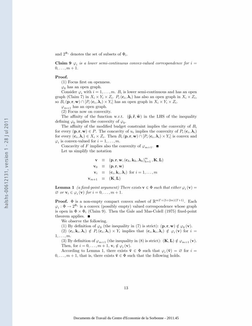
and 2Φ denotes the set of subsets of Φ.
Claim 9 is a lower semi-continuous convex-valued correspondence for =
0 + 1.
Proof.
(1) Focus first on openness.
0 has an open graph.
Consider with = 1 . is lower semi-continuous and has an open
graph (Claim 7) in × × . (cλ) has also an open graph in ×,
so (p rw) ∩ [ (cλ)× ] has an open graph in × × .
+1 has an open graph.
(2) Focus now on convexity.
The affinity of the function w.r.t. (p r w) in the LHS of the inequality
defining 0 implies the convexity of 0.
The affinity of the modified budget constraint implies the convexity of
for every (p rw) ∈ . The concavity of implies the convexity of (cλ)
for every (cλ) ∈ × . Then (p rw) ∩ [ (cλ)× ] is convex and
is convex-valued for = 1 .
Concavity of implies also the convexity of +1.
Let us simplify the notation
v ≡ (p rw (ckλ)=1 KL)
v0 ≡ (p rw)
v ≡ (ckλ) for = 1
v+1 ≡ (KL)
Lemma 1 (a fixed-point argument) There exists v ∈ Φ such that either (v) =∅ or v ∈ (v) for = 0 + 1.
Proof. Φ is a non-empty compact convex subset of R+(5+2)(+1). Each
: Φ → 2Φ is a convex (possibly empty) valued correspondence whose graph
is open in Φ× Φ (Claim 9). Then the Gale and Mas-Colell (1975) fixed-point
theorem applies.
We observe the following.
(1) By definition of 0 (the inequality in (7) is strict): (p rw) ∈ 0 (v).
(2) (ckλ) ∈ (cλ) × implies that (ckλ) ∈ (v) for =
1 .
(3) By definition of +1 (the inequality in (8) is strict): (KL) ∈ +1 (v).
Then, for = 0 + 1, v ∈ (v).
According to Lemma 1, there exists v ∈ Φ such that (v) = ∅ for =
0 + 1, that is, there exists v ∈ Φ such that the following holds.
13
Documents de Travail du Centre d'Economie de la Sorbonne - 2011.45
hals
hs-0
0612
131,
ver
sion
1 -
28 J
ul 2
011
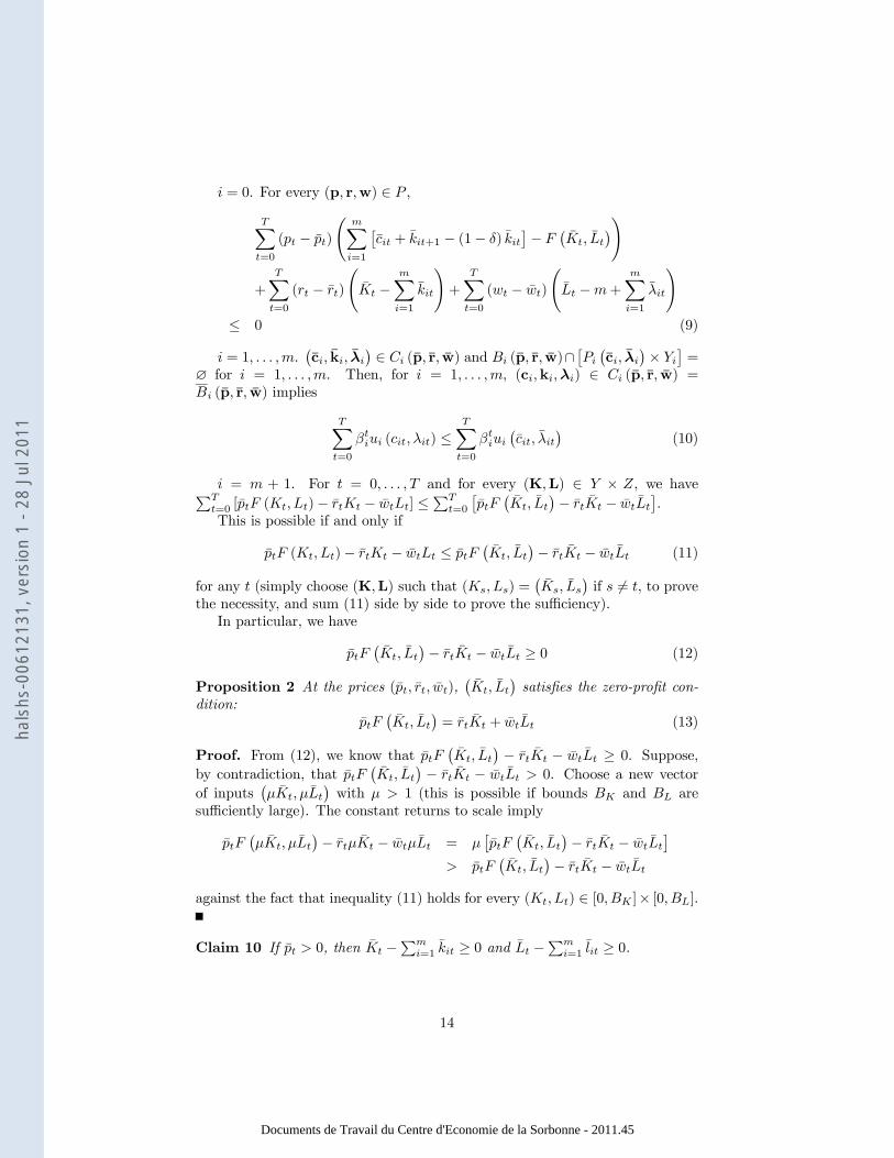
= 0. For every (p rw) ∈ ,
X=0
( − )
ÃX=1
£ + +1 − (1− )
¤− ¡
¢!
+
X=0
( − )
à −
X=1
!+
X=0
( − )
à −+
X=1
!≤ 0 (9)
= 1 .¡c k λ
¢ ∈ (p r w) and (p r w)∩£¡c λ
¢× ¤=
∅ for = 1 . Then, for = 1 , (ckλ) ∈ (p r w) =
(p r w) implies
X=0
( ) ≤X=0
¡
¢(10)
= + 1. For = 0 and for every (KL) ∈ × , we haveP=0 [ ( )− − ] ≤
P=0
£
¡
¢− − ¤.
This is possible if and only if
( )− − ≤ ¡
¢− − (11)
for any (simply choose (KL) such that ( ) =¡
¢if 6= , to prove
the necessity, and sum (11) side by side to prove the sufficiency).
In particular, we have
¡
¢− − ≥ 0 (12)
Proposition 2 At the prices ( ),¡
¢satisfies the zero-profit con-
dition:
¡
¢= + (13)
Proof. From (12), we know that ¡
¢ − − ≥ 0. Suppose,by contradiction, that
¡
¢ − − 0. Choose a new vector
of inputs¡
¢with 1 (this is possible if bounds and are
sufficiently large). The constant returns to scale imply
¡
¢− − = £
¡
¢− − ¤
¡
¢− −
against the fact that inequality (11) holds for every ( ) ∈ [0 ]× [0 ].
Claim 10 If 0, then −P
=1 ≥ 0 and −P
=1 ≥ 0.
14
Documents de Travail du Centre d'Economie de la Sorbonne - 2011.45
hals
hs-0
0612
131,
ver
sion
1 -
28 J
ul 2
011
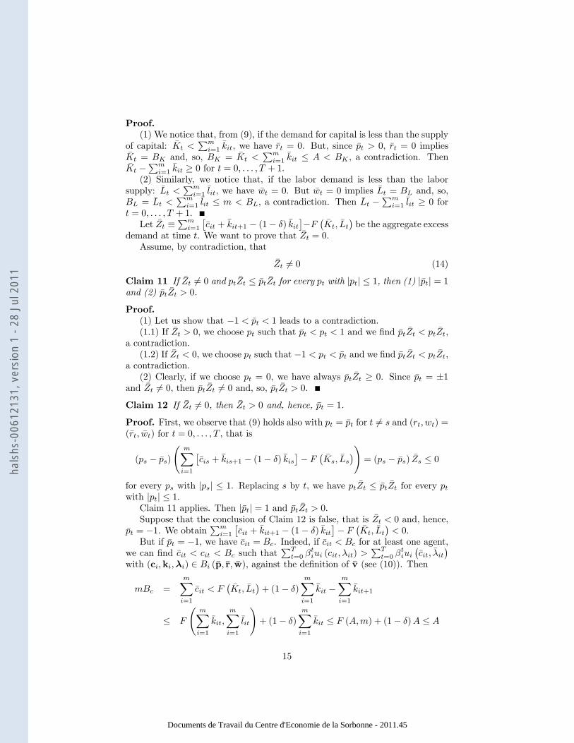
Proof.
(1) We notice that, from (9), if the demand for capital is less than the supply
of capital: P
=1 , we have = 0. But, since 0, = 0 implies
= and, so, = P
=1 ≤ , a contradiction. Then
−P
=1 ≥ 0 for = 0 + 1.(2) Similarly, we notice that, if the labor demand is less than the labor
supply: P
=1 , we have = 0. But = 0 implies = and, so,
= P
=1 ≤ , a contradiction. Then −P
=1 ≥ 0 for = 0 + 1.
Let ≡P
=1
£ + +1 − (1− )
¤− ¡ ¢be the aggregate excess
demand at time . We want to prove that = 0.
Assume, by contradiction, that
6= 0 (14)
Claim 11 If 6= 0 and ≤ for every with || ≤ 1, then (1) || = 1and (2) 0.
Proof.
(1) Let us show that −1 1 leads to a contradiction.
(1.1) If 0, we choose such that 1 and we find ,
a contradiction.
(1.2) If 0, we choose such that −1 and we find ,
a contradiction.
(2) Clearly, if we choose = 0, we have always ≥ 0. Since = ±1and 6= 0, then 6= 0 and, so, 0.Claim 12 If 6= 0, then 0 and, hence, = 1.
Proof. First, we observe that (9) holds also with = for 6= and ( ) =
( ) for = 0 , that is
( − )
ÃX=1
£ + +1 − (1− )
¤− ¡
¢!= ( − ) ≤ 0
for every with || ≤ 1. Replacing by , we have ≤ for every with || ≤ 1.Claim 11 applies. Then || = 1 and 0.
Suppose that the conclusion of Claim 12 is false, that is 0 and, hence,
= −1. We obtainP
=1
£ + +1 − (1− )
¤− ¡
¢ 0.
But if = −1, we have = . Indeed, if for at least one agent,
we can find such thatP
=0 ( )
P=0
¡
¢with (ckλ) ∈ (p r w), against the definition of v (see (10)). Then
=
X=1
¡
¢+ (1− )
X=1
−X=1
+1
≤
ÃX=1
X=1
!+ (1− )
X=1
≤ () + (1− ) ≤
15
Documents de Travail du Centre d'Economie de la Sorbonne - 2011.45
hals
hs-0
0612
131,
ver
sion
1 -
28 J
ul 2
011
a contradiction.
Proposition 3 The goods market clears: = 0, that is
X=1
£ + +1 − (1− )
¤=
¡
¢Proof. = 1 implies ( ) = 0. In this case,
¡c k λ
¢ ∈ (p r w)
implies £ + +1 − (1− )
¤ ≤ +
¡1−
¢and, therefore, we have
X=1
£ + +1 − (1− )
¤ ≤
X=1
+
X=1
(15)
Assume, by contradiction, 6= 0. Claim 12 implies = 1 and 0.
This implies, in turn,
X=1
£ + +1 − (1− )
¤
¡
¢According to (12), we have also
¡
¢ ≥ + .
Finally, we know that ≥P
=1 and ≥P
=1 (Claim 10).
Putting together, we have P
=1
£ + +1 − (1− )
¤
P=1 +
P=1 , in contradiction with (15). Thus the inequality (14) is false and
= 0.
We observe that
X=1
= ¡
¢+
X=1
£(1− ) − +1
¤≤
ÃX=1
X=1
!+ (1− )
X=1
≤ () + (1− ) ≤
We have now to prove that also the capital and the labor markets clear.
Proposition 4 0, = 0 .
Proof. Let us show that 0. Indeed, if ≤ 0, then = for every andP=1
¡ + +1
¢ ≥ ()+ (1− ) ≥ ¡
¢+(1− )
P=1
in contradiction with = 0.
Recall that
( )− − ≥ ( )− −
for any pair ( ) with ≥ 0. Assume = 0 and ≥ 0. In this case,given 0, we have ( )− − = ( )− → +∞if → +∞, since 0: a contradiction. A similar proof works when = 0
and ≥ 0.
16
Documents de Travail du Centre d'Economie de la Sorbonne - 2011.45
hals
hs-0
0612
131,
ver
sion
1 -
28 J
ul 2
011
Proposition 5 =P
=1 and =P
=1 .
Proof. Since 0, we have ≥P
=1 (Claim 10). If P
=1 ,
from (9), we have = 1 0. Then
X=1
£ + +1 − (1− )
¤=
¡
¢ ≥ +
X=1
+
X=1
But¡c k λ
¢ ∈ (p r w) implies P
=1
£ + +1 − (1− )
¤ ≤P
=1 +
P=1
¡1−
¢, a contradiction. Then =
P=1 .
We know that ≥P
=1 (Claim 10). If P
=1 , we have = 1
0. Then
X=1
£ + +1 − (1− )
¤=
¡
¢ ≥ +
X=1
+
X=1
But¡c k λ
¢ ∈ (p r w) implies P
=1
£ + +1 − (1− )
¤ ≤P
=1 +
P=1
¡1−
¢, a contradiction. Then =
P=1 .
We observe thatP
=1 ≤ andP
=1 ≤ .
Proposition 6 The modified budget constraint at equilibrium is a budget con-
straint: ( ) = 0 for = 0 .
Proof. 0 implies that the modified budget constraint is binding:
£ + +1 − (1− )
¤= + + ( )
This gives
X=1
£ + +1 − (1− )
¤=
X=1
+
X=1
+ ( )
Proposition 3 implies ¡
¢=
P=1 +
P=1 + ( ),
while Propositions 2 and 5 entail ¡
¢=
P=1 +
P=1 .
So, ( ) = 0.
Corollary 1¡p r w
¡c k λ
¢=1
K L¢is an equilibrium for the finite-
horizon bounded economy E .
17
Documents de Travail du Centre d'Economie de la Sorbonne - 2011.45
hals
hs-0
0612
131,
ver
sion
1 -
28 J
ul 2
011
9 Appendix 2: infinite horizon
We want to prove Theorem 5. From now on, any variable with subscript
and superscript will refer to a period in a -truncated economy with = 0
if . As above, sequences will be denoted in bold type.
Under the Assumptions 1, 2, 3 and 5 an equilibrium¡p r w
¡c k λ
¢=1
K L¢
of a truncated economy exists. Under these assumptions, namely separability
and differentiability of preferences, the following necessary conditions hold for
the existence of an equilibrium in a truncated economy.
Claim 13 Under Assumption 5, the equilibrium of a truncated economy satis-
fies the following conditions.
For = 0 :
(1)
0 with + +
= 1 (normalization),
(2) ()¡
¢=
,
(3) ()¡
¢=
,
(4) =
P=1
,
(5) =P
=1 ,
(6)P
=1
£ + +1 − (1− )
¤=
¡
¢with +1 = 0.
For = 1 , = 0 :
(7) 0
¡¢=
≥ +1
+1 (1− ) + +1
+1, with equality when
+1 0,
(8) 0³
´≥ 0
¡¢
, with equality when
1,
(9) £ + +1 − (1− )
¤=
+
³1−
´with ≥ 0, +1 =
0 and 0 ≤
≤ 1,where is the multiplier associated to the budget constraint at time .
Proof. See Bosi and Seegmuller (2010) among others.
In the following claims, we omit for simplicity any reference to Assumptions
1, 2, 3 and 5. We suppose that they are always satisfied.
Let us introduce some new variables:
≡ 0
¡¢ if ≤ , and
= 0 if ,
≡ 0
³
´
if ≤ , and = 0 if ,
≡ 0
³
´if ≤ , and
= 0 if ,
≡ if ≤ , and
= 0 if ,
(16)
and ≡
−
.
We notice that points (7) and (8) of Claim 13 entail ≥ 0 and = 0
when
1.
18
Documents de Travail du Centre d'Economie de la Sorbonne - 2011.45
hals
hs-0
0612
131,
ver
sion
1 -
28 J
ul 2
011
Claim 14 For any 0, there exists such that, for any and for any
,P∞
=
.
We observe that the critical is independent of .
Proof. We know that, under Assumptions 1 and 2, ≤ and ≤ . We
observe thatP∞
=0 () = () (1− ) ∞. Then, there exists such
thatP∞
= () . In addition, under Assumption 5,
∞X=
() ≥X=
¡¢=
X=
£¡¢− (0)
¤≥
X=
0
¡¢ (17)
because of the concavity of . Thus, for any 0, there exists such that,
for any and for any ,P∞
=
.
Claim 15 For any 0, there exists such that, for any and for any
,P∞
= .
As above, the critical does not depend on .
Proof. SinceP∞
=0 (1) = (1) (1− ) ∞, there exists such thatP∞
= (1) . In addition, under Assumption 5,
∞X=
(1) ≥X=
³
´=
X=
h
³
´− (0)
i≥
X=
0
³
´
(18)
because
≤ 1 and is concave. Thus, for any 0, there exists such that,for any and for any ,
P∞=
.
Notice that, as above, the critical does not depend on .
Claim 16 For any 0, there exists such that, for any and for any
,P∞
=
andP∞
= . In addition, for any ,
³
´∞=0∈ 1+
and¡¢∞=0∈ 1+.
Notice that the critical does not depend on .
Proof. From (16), we observe that 0
³
´
=
+
=
+
since = 0 when
1. For any 0, there exists such that, for any ,P∞=
(1) . Thus, according to (18), for any 0, there exists such
that, for any and for any ,P
=
³
+
´=P
= 0
³
´
. In particular,P∞
=
andP∞
= .
19
Documents de Travail du Centre d'Economie de la Sorbonne - 2011.45
hals
hs-0
0612
131,
ver
sion
1 -
28 J
ul 2
011
From (18), we have also, for any ,
∞X=0
³
+
´≤∞X=0
(1) = (1) (1− )
and, so,P∞
=0
≤ (1) (1− ) andP∞
=0 ≤ (1) (1− ). Then,
for any ,³
´∞=0∈ 1+ and
¡¢∞=0∈ 1+.
Claim 17 For any 0 there exists such that for any and any ≥
we haveP
=
. In addition, for any ,
X=0
() + (1)
1− (19)
Proof. Focus now on the sequence of equilibrium budget constraints: +
³1−
´−
£ + +1 − (1− )
¤ ≥ 0.Multiplying them by the multipliers, we obtain, according to the Kuhn-
Tucker method,
+
³1−
´−
−
+1 +
(1− ) = 0 (20)
Summing them over time from = to = , we get
+
³1−
´−
−
+1 +
(1− )
++1+1
+1 + +1
+1
³1−
+1
´− +1
+1
+1
−+1+1+2 + +1+1 (1− ) +1
+
+
+
³1−
´−
−
+1
+ (1− )
= 0
that is
X=
−X=
−−1X=
£
− +1
+1 (1− )− +1
+1
¤+1
+ (1− ) +
−
+1
=
X=
=
X=
0
¡¢ =
X=
20
Documents de Travail du Centre d'Economie de la Sorbonne - 2011.45
hals
hs-0
0612
131,
ver
sion
1 -
28 J
ul 2
011
We know that£
− +1
+1 (1− )− +1
+1
¤+1 = 0 because ei-
ther − +1
+1 (1− )− +1
+1 = 0 or
+1 = 0 (point (7) of Claim
13). Then
X=
=
X=
+
X=
− (1− ) − +
+1
(21)
From the proof of Claim 14, we know that
X=
≤X=
() = () − +1
1−
()
1− (22)
Thus, for any 0, there exists 1 such that, for any 1 and for any
≥ ,X=
2 (23)
From the proof of Claim 16, we know also that
X=
≤X=
(1) = (1) − +1
1−
(1)
1− (24)
Thus, for any 0, there exists 2 such that, for any 2 and for any
≥ ,X=
2
According to (21), we have that
X=
≤X=
+
X=
+
+1
=
X=
+
X=
(25)
because in the truncated economy +1 = 0.
Thus, for any 0, there exists ≡ max {1 2} such that, for any
and for any ≥ ,X=
2 + 2 =
because in the truncated economy +1 = 0.
21
Documents de Travail du Centre d'Economie de la Sorbonne - 2011.45
hals
hs-0
0612
131,
ver
sion
1 -
28 J
ul 2
011
Finally, from (22), (24) and (25), we have
X=
≤X=
+
X=
[ () + (1)]
1−
Taking = 0, we obtain (19).
Claim 18 Let ϑ
≡³
´∞=0. There is a subsequence
³ϑ
´∞=0
which con-
verges for the 1-topology to a sequence ϑ ≡¡¢∞=0∈ 1+. The limit ϑ shares
the same properties of the terms ϑ
of the sequence, namely, (1) for any 0
there exists (the same for all the terms) such that, for any , we haveP∞= ≤ , and (2)
P∞=0 ≤ [ () + (1)] (1− ).
Proof. We apply Claim 17 and we find that, for any 0 there exists such
that for any and for any , we haveP∞
=
≤ . We observe also that
(19) impliesP∞
=0
≤ [ () + (1)] (1− ) for any . Thus, Lemma 2 in
Appendix 3 applies with a ball of radius = [ () + (1)] (1− ).
Claim 19 In the infinite-horizon economy, leisure demand is positive:
lim→∞
= ∈ (0 1]
Proof. We have
=
+ with ≥ 0 and = 0 if
1.
From Claim 17, we know that, for any 0, there exists 1 such that, for
any 1 and for any ,P∞
=
≤ 2.
From Claim 16, we know that for any 0, there exists 2 such that, for
any 2 and for any ,P∞
= 2.
Hence, for any 0, there exists ≡ max {1 2} such that, for any
and for any ,P∞
=
=P∞
=
+P∞
= . In addition, for any ,
∞X=0
=
∞X=0
+
∞X=0
≤ () + (1)
1− +
(1)
1−
Let θ
≡³
´. Then θ
→ θ ∈ 1+ for the 1-topology (Lemma 2 in
Appendix 3 applies with = [ () + 2 (1)] (1− )).
Therefore, for any ,
converges to ∈ (0+∞). Hence, converges to 0 since satisfies the Inada conditions (Assumption 5). Clearly, ≤ 1.
Claim 20 In the infinite-horizon economy, the equilibrium prices are positive:
lim→∞ = ∈ (0 1), lim→∞ = ∈ (0 1), lim→∞ = ∈ (0 1).
22
Documents de Travail du Centre d'Economie de la Sorbonne - 2011.45
hals
hs-0
0612
131,
ver
sion
1 -
28 J
ul 2
011
Proof. Focus on prices.
Suppose that lim→∞ = 0. We know that 0
¡¢=
.
If is bounded, we have lim→∞ 0¡¢= 0 which is impossible because
≤ for every .
Then, lim→∞ = +∞. However, 0
³
´ =
+ and
lim→∞ = lim→∞
³
´− lim→∞
¡
¢= 0 (Claim 19).
Since lim→∞ = 0, lim→∞ = 0 and +
+ = 1, we get
lim→∞ = 1.
We know that −1−1 ≥
(1− )+
≥
(point (7) of Claim
13). Then lim→∞ −1−1 ≥ lim→∞
= +∞.
Similarly, −2−2 ≥ −1
−1 (1− ) + −1
−1 ≥ −1
−1 (1− ) and
lim→∞ −2−2 ≥ lim→∞ −1
−1 (1− ) = +∞.
Computing backward, we obtain lim→∞ 00 = +∞.
If lim→∞ 0 0, since 0 ≤ 1, then lim→∞ 0 = +∞ and, since
lim→∞ 00 = 0 +∞, this implies lim→∞
0 = 0. Thus,
0 = 0¡0 0
¢− 00 − 00 = 0¡0 0
¢− 00
Choose 0 0 in order to obtain a strictly higher profit and a contradiction
with profit maximization.
Let lim→∞ 0 = 0. We know that 0 () ≤ 0
¡0¢= 0
0
¡0¢= 0
0 .
If lim→∞ 0 +∞, we have lim→∞ 00 = 0 and 0 () ≤ 0, a contra-
diction.
If lim→∞ 0 = +∞, then lim→∞ 00 = 0 +∞ gives lim→∞
0 =
0 and lim→∞ 0 = 1. Focus on the first budget constraint:
0£0 + 1 − (1− ) 0
¤= 0 0 +
0
³1−
0
´Assumption 3 ensures 0 0. In this case, in the limit:
0 = 0£0 + 1 − (1− ) 0
¤= 00 + 0
¡1− 0
¢ ≥ 0 0
a contradiction. Thus, for every , → 0.
Focus now on and . In the limit, ¡
¢− − = 0.
If = 0, then ¡
¢ − = 0. Fix 0 and choose large
enough such that ( )− 0, against the equilibrium condition.
If = 0, then ¡
¢ − = 0. Fix 0 and choose large
enough such that ( )− 0, against the equilibrium condition.
Thus, 0.
Claim 21 = lim→∞ ∈ (0+∞).Proof. For any ,
P=1
≤ . This implies ≤ independently on the
choice of and lim→∞ ≤ +∞. In addition, if = lim→∞ = 0,
then, since 0¡¢
≤ 0
³
´, we obtain+∞ = lim→∞ 0
¡¢
≤
lim→∞ 0³
´, that is = lim→∞
= 0, a contradiction (see Claim 19).
Then 0.
23
Documents de Travail du Centre d'Economie de la Sorbonne - 2011.45
hals
hs-0
0612
131,
ver
sion
1 -
28 J
ul 2
011
Claim 22 For any , lim→∞ = 0 and lim→∞ = 0.
Proof. We know thatP
=1 +1 ≥ 0 and thatP
=1 +P
=1 +1 =
¡
¢+ (1− ) . If = 0, then = 0 for every , a contradiction.
Now, if = 0, we have = 0 and hence = 0: a contradiction.
Claim 23 lim→+∞ +1 = 0.
Proof. Let 0. We know that there exists such that for any pair
( 0) such that 0 and for any , we haveP0
=
andP0
=
³1−
´ for every (inequality (23) and Claim 17). Taking the
limit for → +∞, we get also
≥ lim→+∞
0X=
=
0X=
lim→+∞
£
0
¡¢¤=
0X=
0 ()
=
0X=
(see Claim 21) and
≥ lim→+∞
0X=
³1−
´=
0X=
lim→+∞
¡
¢µ1− lim
→+∞
¶
=
0X=
¡1−
¢(see Claims 18 and 19). Since this holds for any 0 , we get also
∞X=
≤ and
∞X=
¡1−
¢ ≤ (26)
From the budget constraints, for any 0 ≥ , we obtain
0X=
=
(1− ) +
+
0X=
³1−
´≥
(1− ) +
(see (21)). Taking the limit for → +∞, we obtain (1− ) ≤ and ≤
for every . Thus, lim sup (1− ) ≤ and lim sup ≤ .
These inequalities hold for any 0. Hence
lim→+∞
(1− ) = 0 and lim→+∞
= 0 (27)
24
Documents de Travail du Centre d'Economie de la Sorbonne - 2011.45
hals
hs-0
0612
131,
ver
sion
1 -
28 J
ul 2
011
Again, from the budget constraint, we have
+1 =
(1− ) +
+
³1−
´−
(see (20)). Taking the limit for → +∞,
we obtain +1 = (1− ) + +
¡1−
¢− . Weknow that lim→+∞ (1− ) = 0 and lim→+∞ = 0 (see (27)).
We know also that lim→+∞
¡1−
¢= 0 and lim→+∞ = 0 (see
(26)). Therefore, lim→+∞ +1 = 0.
Claim 24¡p r w
¡c k λ
¢=1
k L¢is an equilibrium.
Proof. Consider first the firm. For every truncated -economy a zero profit
condition holds: ¡
¢ − −
= 0. In the limit, for the
infinite-horizon economy: ¡
¢ − − = 0, because → ∈
(0 1), → ∈ (0 1), → ∈ (0 1), =
P=1
→
P=1 =
+∞, =P
=1 →
P=1 = +∞. If
¡
¢does not
maximize the profit in the infinite-horizon economy, then there exists ( )
such that ( ) − − ¡
¢ − − = 0 and,
so, a critical , such that, for any , ( ) − −
¡
¢− −
= 0 against the fact that
¡
¢maximizes
the profit in the -economy.
Focus on the consumer. Consider an alternative sequence (ckλ) which
satisfies the budget constraints and the Euler inequalities in the infinite-horizon
economy. We have
∆ ≡X=0
£ () +
¡¢¤− X
=0
[ () + ()]
=
X=0
[ ()− ()] +
X=0
£¡¢− ()
¤≥
X=0
0 () ( − ) +
X=0
0
¡¢ ¡ −
¢≥
X=0
( − ) +
X=0
¡ −
¢We observe that
−
¡1−
¢= + (1− ) − +1
− (1− ) ≤ + (1− ) − +1
where the first equality holds because of the Kuhn-Tucker method.
Subtracting member by member, we get
( − ) +
¡ −
¢≥ £
+ (1− ) − +1¤
− [ + (1− ) − +1]
25
Documents de Travail du Centre d'Economie de la Sorbonne - 2011.45
hals
hs-0
0612
131,
ver
sion
1 -
28 J
ul 2
011
Summing over , we obtain
X=0
( − ) +
X=0
¡ −
¢≥
X=0
£ (1− ) + − +1
¤−
X=0
[ (1− ) + − +1]
We know also that£ − +1+1 (1− )− +1+1
¤+1 = 0£
− +1+1 (1− )− +1+1¤+1 = 0
(point (7) in the Claim 13), that is
(1− ) + = −1−1 (1− ) + = −1−1
Then
X=0
( − ) +
X=0
¡ −
¢=
X=0
¡−1−1 − +1
¢− X=0
¡−1−1 − +1
¢= −1−10 − +1 −
£−1−10 − +1
¤= − +1 + +1
≥ − +1Thus lim→+∞∆ ≥ 0 (Claim 23) and
∞X=0
£ () +
¡¢¤ ≥ ∞X
=0
[ () + ()]
Thus¡c λ
¢maximizes the consumer’s objective.
10 Appendix 3
Let (0 ) ≡ ©x ∈ 1 :P∞
=0 || ≤ ªbe a ball of 1.
Lemma 2 Let be a subset of (0 ), which satisfies the property: for any
0, there exists such that for any and for any x ∈ ,P∞
= || ≤ .
Then is compact for the 1-topology.
26
Documents de Travail du Centre d'Economie de la Sorbonne - 2011.45
hals
hs-0
0612
131,
ver
sion
1 -
28 J
ul 2
011
Proof. Let¡y¢be a sequence in . (0 ) is a compact set for the product
topology and contains the sequence¡y¢. Thus there exists a subsequence¡
y¢which, for the product topology, converges to some y ∈ (0 ).
For any 0, there exists such that for any and for any ,P∞=
¯
¯≤ . Take now any 0 . We have, for any 0, for any and
for any ,P0
=
¯
¯≤P∞= ¯ ¯
≤ . Convergence of¡y
¢for the product
topology implies, for any 0 and for any ,P0
= || ≤ . Thus we get, for
any ,P∞
= || ≤ . Then y ∈ and is compact for the 1-topology.
References
[1] Becker R.A. (1980). On the long-run steady state in a simple dynamic
model of equilibrium with heterogeneous households. Quarterly Journal of
Economics 95, 375-382.
[2] Becker R.A. (2005). An example of optimal growth with heterogeneous
agents and twisted turnpike. Mimeo, Indiana University.
[3] Becker R.A. (2006). Equilibrium dynamics with many agents. In Dana R.-
A., C. Le Van, T. Mitra and K. Nishimura eds., Handbook of Optimal
Growth 1, Springer Verlag, 385-442.
[4] Becker R.A., J. H. Boyd III and C. Foias (1991). The existence of Ramsey
equilibrium. Econometrica 59, 441-460.
[5] Becker R.A. and C. Foias (1987). A characterization of Ramsey equilibrium.
Journal of Economic Theory 41, 173-184.
[6] Becker R.A. and C. Foias (1994). The local bifurcation of Ramsey equilib-
rium. Economic Theory 4, 719-744.
[7] Becker R.A. and C. Foias (2007). Strategic Ramsey equilibrium dynamics.
Journal of Mathematical Economics 43, 318-346.
[8] Bergstrom T.C. (1976). How to discard "free disposability" - at no cost.
Journal of Mathematical Economics 3, 131-134.
[9] Bosi S. and T. Seegmuller (2010). On the Ramsey equilibrium with hetero-
geneous consumers and endogenous labor supply. Journal of Mathematical
Economics 46, 475-492.
[10] Florenzano M. (1999). General equilibrium of financial markets: an intro-
duction. Cahiers de la MSE 1999.76, University of Paris 1.
[11] Gale D. and A. Mas-Colell (1975). An equilibrium existence theorem for a
general model without ordered preferences. Journal of Mathematical Eco-
nomics 2, 9-15.
27
Documents de Travail du Centre d'Economie de la Sorbonne - 2011.45
hals
hs-0
0612
131,
ver
sion
1 -
28 J
ul 2
011
[12] Gale D. and A. Mas-Colell (1979). Corrections to an equilibrium existence
theorem for a general model without ordered preferences. Journal of Math-
ematical Economics 6, 297-298.
[13] Le Van C., M.H. Nguyen and Y. Vailakis (2007). Equilibrium dynamics in
an aggregative model of capital accumulation with heterogeneous agents
and elastic labor. Journal of Mathematical Economics 43, 287-317.
[14] Le Van C. and Y. Vailakis (2003). Existence of a competitive equilibrium
in a one sector growth model with heterogeneous agents and irreversible
investment. Economic Theory 22, 743-771.
[15] Mitra T. (1979). On optimal economic growth with variable discount rates:
existence and stability results. International Economic Review 20, 133-145.
[16] Ramsey F.P. (1928). A mathematical theory of saving. Economic Journal
38, 543-559.
[17] Sarte P.-D. (1997). Progressive taxation and income inequality in dynamic
competitive equilibrium. Journal of Public Economics 66, 145-171.
[18] Sorger G. (1994). On the structure of Ramsey equilibrium: cycles, indeter-
minacy, and sunspots. Economic Theory 4, 745-764.
[19] Sorger G. (2002). On the long-run distribution of capital in the Ramsey
model. Journal of Economic Theory 105, 226-243.
[20] Sorger G. (2005). Differentiated capital and the distribution of wealth. In
Deissenberg C. and R.F. Hartl eds., Optimal Control and Dynamic Games,
Springer Verlag, 177-196.
[21] Sorger G. (2008). Strategic saving decisions in the infinite-horizon model.
Economic Theory 36, 353-377.
28
Documents de Travail du Centre d'Economie de la Sorbonne - 2011.45
hals
hs-0
0612
131,
ver
sion
1 -
28 J
ul 2
011
Recommended