Homogénéisation delois de conservation scalaires
Anne-Laure Dalibard
CEREMADEUniversité Paris-Dauphine
06 Avril 2007Séminaire de Mathématiques Appliquées
du Collège de France
Outline
1. Introduction
2. The viscous case : study of the homogenized problem
3. The viscous case : convergence proof
4. The hyperbolic case
Outline
1. Introduction
2. The viscous case : study of the homogenized problem
3. The viscous case : convergence proof
4. The hyperbolic case
Outline
1. Introduction
2. The viscous case : study of the homogenized problem
3. The viscous case : convergence proof
4. The hyperbolic case
Outline
1. Introduction
2. The viscous case : study of the homogenized problem
3. The viscous case : convergence proof
4. The hyperbolic case
1. Introduction
Outline
1. Introduction
2. The viscous case : study of the homogenized problem
3. The viscous case : convergence proof
4. The hyperbolic case
1. Introduction
Setting of the problem
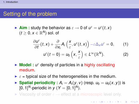
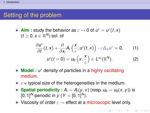
I Aim : study the behavior as ε→ 0 of uε = uε(t , x)(t ≥ 0, x ∈ RN ) sol. of
∂uε
∂t(t , x) +
∂
∂xiAi
(xε,uε(t , x)
)−ε∆xuε = 0, (1)
uε(t = 0) = u0
(x ,
xε
)∈ L∞(RN). (2)
I Model : uε density of particles in a highly oscillatingmedium.
I ε = typical size of the heterogeneities in the medium.I Spatial periodicity : Ai = Ai(y , v) (resp. u0 = u0(x , y)) is
[0,1]N -periodic in y (Y = [0,1]N ).I Viscosity of order ε→ effect at a microscopic level only.
1. Introduction
Setting of the problem
I Aim : study the behavior as ε→ 0 of uε = uε(t , x)(t ≥ 0, x ∈ RN ) sol. of
∂uε
∂t(t , x) +
∂
∂xiAi
(xε,uε(t , x)
)−ε∆xuε = 0, (1)
uε(t = 0) = u0
(x ,
xε
)∈ L∞(RN). (2)
I Model : uε density of particles in a highly oscillatingmedium.
I ε = typical size of the heterogeneities in the medium.I Spatial periodicity : Ai = Ai(y , v) (resp. u0 = u0(x , y)) is
[0,1]N -periodic in y (Y = [0,1]N ).I Viscosity of order ε→ effect at a microscopic level only.
1. Introduction
Goals and tools
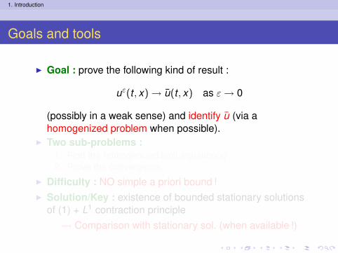
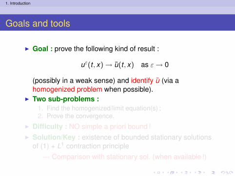
I Goal : prove the following kind of result :
uε(t , x) → u(t , x) as ε→ 0
(possibly in a weak sense) and identify u (via ahomogenized problem when possible).
I Two sub-problems :1. Find the homogenized/limit equation(s) ;2. Prove the convergence.
I Difficulty : NO simple a priori bound !I Solution/Key : existence of bounded stationary solutions
of (1) + L1 contraction principle→ Comparison with stationary sol. (when available !)
1. Introduction
Goals and tools
I Goal : prove the following kind of result :
uε(t , x) → u(t , x) as ε→ 0
(possibly in a weak sense) and identify u (via ahomogenized problem when possible).
I Two sub-problems :1. Find the homogenized/limit equation(s) ;2. Prove the convergence.
I Difficulty : NO simple a priori bound !I Solution/Key : existence of bounded stationary solutions
of (1) + L1 contraction principle→ Comparison with stationary sol. (when available !)
1. Introduction
Previous works
I Weinan E ; Weinan E and D. Serre (1992).I Y. Amirat, K. Hamdache and A. Ziani (1989).I L. Dumas and F. Golse (2000).I P.-E. Jabin and A. E. Tzavaras (recent work).I N = 1,2 : equivalence with Hamilton-Jacobi equations.
P.-L. Lions, G. Papanicolaou, S.R.S. Varadhan (1987) ; L.C.Evans (1992).
2. The viscous case : study of the homogenized problem
Outline
1. Introduction
2. The viscous case : study of the homogenized problema. Ansatz - Formal derivationb. Cell problemc. Initial layer
3. The viscous case : convergence proof
4. The hyperbolic case
2. The viscous case : study of the homogenized problem
a. Ansatz - Formal derivation
Outline
1. Introduction
2. The viscous case : study of the homogenized problema. Ansatz - Formal derivationb. Cell problemc. Initial layer
3. The viscous case : convergence proof
4. The hyperbolic case
2. The viscous case : study of the homogenized problem
a. Ansatz - Formal derivation
Formal asymptotic expansionCell problem
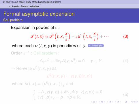
Expansion in powers of ε :
uε(t , x) ≈ u0(
t , x ,xε
)+ εu1
(t , x ,
xε
)+ · · · (3)
where each ui(t , x , y) is periodic w.r.t. y . To hyp. pb.
Order ε−1 : Cell problem :
−∆yu0 + divyA(y ,u0) = 0, y ∈ Y . (4)
→ Re-write u0(t , x , y) as
u0(t , x , y) = v(y , u(t , x))
where u(t , x) =⟨u0(t , x , ·)
⟩Y and{
−∆yv(y ,p) + divyA(y , v(y ,p)) = 0,〈v(·,p)〉Y = p ∀p ∈ R. (5)
2. The viscous case : study of the homogenized problem
a. Ansatz - Formal derivation
Formal asymptotic expansionCell problem
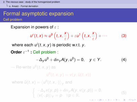
Expansion in powers of ε :
uε(t , x) ≈ u0(
t , x ,xε
)+ εu1
(t , x ,
xε
)+ · · · (3)
where each ui(t , x , y) is periodic w.r.t. y .
Order ε−1 : Cell problem :
−∆yu0 + divyA(y ,u0) = 0, y ∈ Y . (4)
→ Re-write u0(t , x , y) as
u0(t , x , y) = v(y , u(t , x))
where u(t , x) =⟨u0(t , x , ·)
⟩Y and{
−∆yv(y ,p) + divyA(y , v(y ,p)) = 0,〈v(·,p)〉Y = p ∀p ∈ R. (5)
2. The viscous case : study of the homogenized problem
a. Ansatz - Formal derivation
Formal asymptotic expansionCell problem
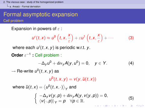
Expansion in powers of ε :
uε(t , x) ≈ u0(
t , x ,xε
)+ εu1
(t , x ,
xε
)+ · · · (3)
where each ui(t , x , y) is periodic w.r.t. y .
Order ε−1 : Cell problem :
−∆yu0 + divyA(y ,u0) = 0, y ∈ Y . (4)
→ Re-write u0(t , x , y) as
u0(t , x , y) = v(y , u(t , x))
where u(t , x) =⟨u0(t , x , ·)
⟩Y and{
−∆yv(y ,p) + divyA(y , v(y ,p)) = 0,〈v(·,p)〉Y = p ∀p ∈ R. (5)
2. The viscous case : study of the homogenized problem
a. Ansatz - Formal derivation
Formal asymptotic expansionHomogenized problem
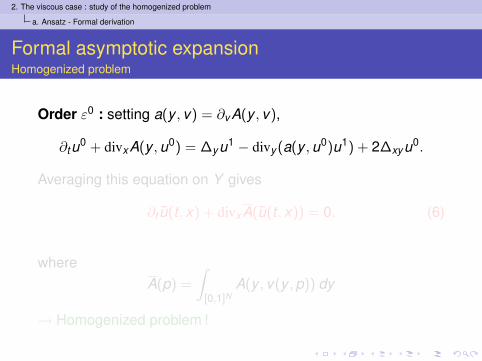
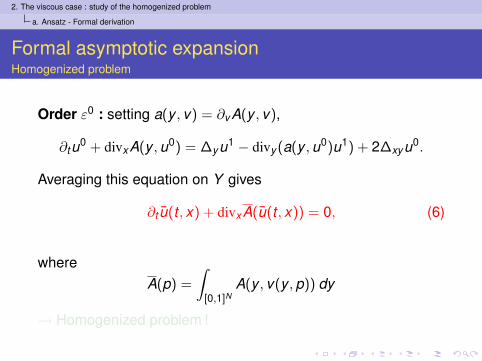
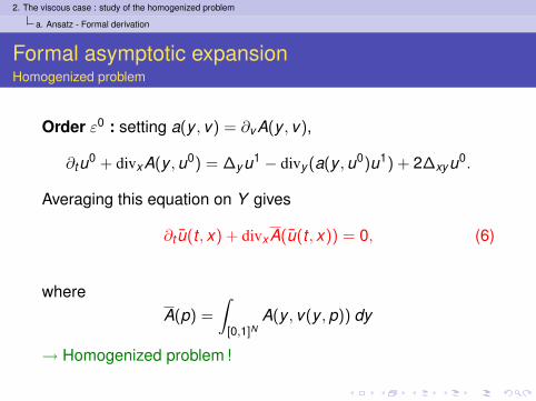
Order ε0 : setting a(y , v) = ∂v A(y , v),
∂tu0 + divxA(y ,u0) = ∆yu1 − divy (a(y ,u0)u1) + 2∆xyu0.
Averaging this equation on Y gives
∂t u(t , x) + divxA(u(t , x)) = 0, (6)
whereA(p) =
∫[0,1]N
A(y , v(y ,p)) dy
→ Homogenized problem !
2. The viscous case : study of the homogenized problem
a. Ansatz - Formal derivation
Formal asymptotic expansionHomogenized problem
Order ε0 : setting a(y , v) = ∂v A(y , v),
∂tu0 + divxA(y ,u0) = ∆yu1 − divy (a(y ,u0)u1) + 2∆xyu0.
Averaging this equation on Y gives
∂t u(t , x) + divxA(u(t , x)) = 0, (6)
whereA(p) =
∫[0,1]N
A(y , v(y ,p)) dy
→ Homogenized problem !
2. The viscous case : study of the homogenized problem
a. Ansatz - Formal derivation
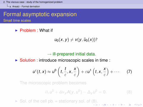
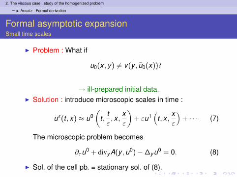
Formal asymptotic expansionSmall time scales
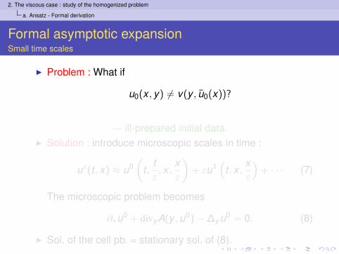
I Problem : What if
u0(x , y) 6= v(y , u0(x))?
→ ill-prepared initial data.I Solution : introduce microscopic scales in time :
uε(t , x) ≈ u0(
t ,tε, x ,
xε
)+ εu1
(t , x ,
xε
)+ · · · (7)
The microscopic problem becomes
∂τu0 + divyA(y ,u0)−∆yu0 = 0. (8)
I Sol. of the cell pb. = stationary sol. of (8).
2. The viscous case : study of the homogenized problem
a. Ansatz - Formal derivation
Formal asymptotic expansionSmall time scales
I Problem : What if
u0(x , y) 6= v(y , u0(x))?
→ ill-prepared initial data.I Solution : introduce microscopic scales in time :
uε(t , x) ≈ u0(
t ,tε, x ,
xε
)+ εu1
(t , x ,
xε
)+ · · · (7)
The microscopic problem becomes
∂τu0 + divyA(y ,u0)−∆yu0 = 0. (8)
I Sol. of the cell pb. = stationary sol. of (8).
2. The viscous case : study of the homogenized problem
b. Cell problem
Outline
1. Introduction
2. The viscous case : study of the homogenized problema. Ansatz - Formal derivationb. Cell problemc. Initial layer
3. The viscous case : convergence proof
4. The hyperbolic case
2. The viscous case : study of the homogenized problem
b. Cell problem
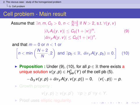
Cell problem - Main result
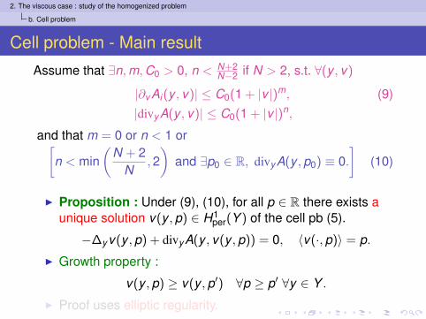
Assume that ∃n,m,C0 > 0, n < N+2N−2 if N > 2, s.t. ∀(y , v)
|∂v Ai(y , v)| ≤ C0(1 + |v |)m, (9)|divyA(y , v)| ≤ C0(1 + |v |)n,
and that m = 0 or n < 1 or[n < min
(N + 2
N,2
)and ∃p0 ∈ R, divyA(y ,p0) ≡ 0.
](10)
I Proposition : Under (9), (10), for all p ∈ R there exists aunique solution v(y ,p) ∈ H1
per(Y ) of the cell pb (5).
−∆yv(y ,p) + divyA(y , v(y ,p)) = 0, 〈v(·,p)〉 = p.
I Growth property :
v(y ,p) ≥ v(y ,p′) ∀p ≥ p′ ∀y ∈ Y .
I Proof uses elliptic regularity.
2. The viscous case : study of the homogenized problem
b. Cell problem
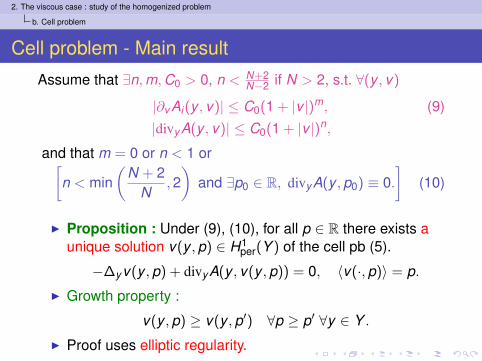
Cell problem - Main result
Assume that ∃n,m,C0 > 0, n < N+2N−2 if N > 2, s.t. ∀(y , v)
|∂v Ai(y , v)| ≤ C0(1 + |v |)m, (9)|divyA(y , v)| ≤ C0(1 + |v |)n,
and that m = 0 or n < 1 or[n < min
(N + 2
N,2
)and ∃p0 ∈ R, divyA(y ,p0) ≡ 0.
](10)
I Proposition : Under (9), (10), for all p ∈ R there exists aunique solution v(y ,p) ∈ H1
per(Y ) of the cell pb (5).
−∆yv(y ,p) + divyA(y , v(y ,p)) = 0, 〈v(·,p)〉 = p.
I Growth property :
v(y ,p) ≥ v(y ,p′) ∀p ≥ p′ ∀y ∈ Y .
I Proof uses elliptic regularity.
2. The viscous case : study of the homogenized problem
b. Cell problem
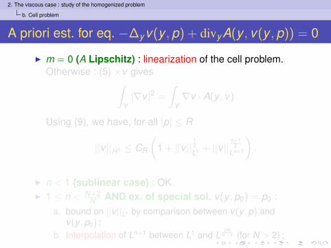
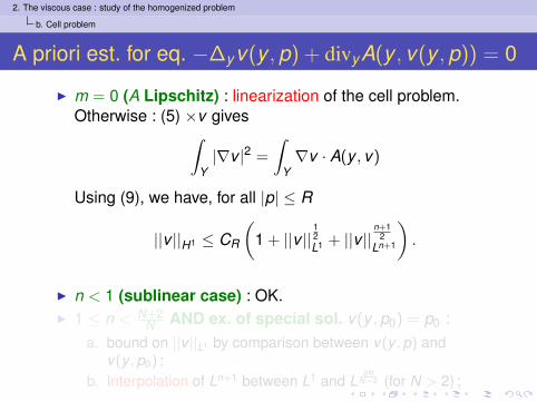
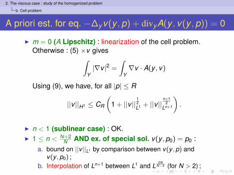
A priori est. for eq. −∆yv(y , p) + divyA(y , v(y , p)) = 0
I m = 0 (A Lipschitz) : linearization of the cell problem.Otherwise : (5) ×v gives∫
Y|∇v |2 =
∫Y∇v · A(y , v)
Using (9), we have, for all |p| ≤ R
||v ||H1 ≤ CR
(1 + ||v ||
12L1 + ||v ||
n+12
Ln+1
).
I n < 1 (sublinear case) : OK.I 1 ≤ n < N+2
N AND ex. of special sol. v(y ,p0) = p0 :a. bound on ||v ||L1 by comparison between v(y ,p) and
v(y ,p0) ;b. Interpolation of Ln+1 between L1 and L
2NN−2 (for N > 2) ;

2. The viscous case : study of the homogenized problem
b. Cell problem
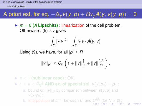
A priori est. for eq. −∆yv(y , p) + divyA(y , v(y , p)) = 0
I m = 0 (A Lipschitz) : linearization of the cell problem.Otherwise : (5) ×v gives∫
Y|∇v |2 =
∫Y∇v · A(y , v)
Using (9), we have, for all |p| ≤ R
||v ||H1 ≤ CR
(1 + ||v ||
12L1 + ||v ||
n+12
Ln+1
).
I n < 1 (sublinear case) : OK.I 1 ≤ n < N+2
N AND ex. of special sol. v(y ,p0) = p0 :a. bound on ||v ||L1 by comparison between v(y ,p) and
v(y ,p0) ;b. Interpolation of Ln+1 between L1 and L
2NN−2 (for N > 2) ;
2. The viscous case : study of the homogenized problem
b. Cell problem
A priori est. for eq. −∆yv(y , p) + divyA(y , v(y , p)) = 0
I m = 0 (A Lipschitz) : linearization of the cell problem.Otherwise : (5) ×v gives∫
Y|∇v |2 =
∫Y∇v · A(y , v)
Using (9), we have, for all |p| ≤ R
||v ||H1 ≤ CR
(1 + ||v ||
12L1 + ||v ||
n+12
Ln+1
).
I n < 1 (sublinear case) : OK.I 1 ≤ n < N+2
N AND ex. of special sol. v(y ,p0) = p0 :a. bound on ||v ||L1 by comparison between v(y ,p) and
v(y ,p0) ;b. Interpolation of Ln+1 between L1 and L
2NN−2 (for N > 2) ;
2. The viscous case : study of the homogenized problem
c. Initial layer
Outline
1. Introduction
2. The viscous case : study of the homogenized problema. Ansatz - Formal derivationb. Cell problemc. Initial layer
3. The viscous case : convergence proof
4. The hyperbolic case
2. The viscous case : study of the homogenized problem
c. Initial layer
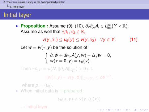
Initial layer
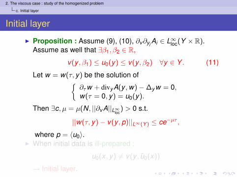
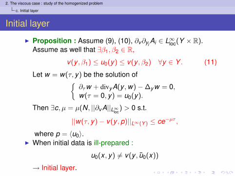
I Proposition : Assume (9), (10), ∂v∂yj Ai ∈ L∞loc(Y × R).Assume as well that ∃β1, β2 ∈ R,
v(y , β1) ≤ u0(y) ≤ v(y , β2) ∀y ∈ Y . (11)
Let w = w(τ, y) be the solution of{∂τw + divyA(y ,w)−∆yw = 0,w(τ = 0, y) = u0(y).
Then ∃c, µ = µ(N, ||∂v A||L∞loc) > 0 s.t.
||w(τ, y)− v(y ,p)||L∞(Y ) ≤ ce−µτ ,
where p = 〈u0〉.I When initial data is ill-prepared :
u0(x , y) 6= v(y , u0(x))
→ Initial layer.
2. The viscous case : study of the homogenized problem
c. Initial layer
Initial layer
I Proposition : Assume (9), (10), ∂v∂yj Ai ∈ L∞loc(Y × R).Assume as well that ∃β1, β2 ∈ R,
v(y , β1) ≤ u0(y) ≤ v(y , β2) ∀y ∈ Y . (11)
Let w = w(τ, y) be the solution of{∂τw + divyA(y ,w)−∆yw = 0,w(τ = 0, y) = u0(y).
Then ∃c, µ = µ(N, ||∂v A||L∞loc) > 0 s.t.
||w(τ, y)− v(y ,p)||L∞(Y ) ≤ ce−µτ ,
where p = 〈u0〉.I When initial data is ill-prepared :
u0(x , y) 6= v(y , u0(x))
→ Initial layer.
2. The viscous case : study of the homogenized problem
c. Initial layer
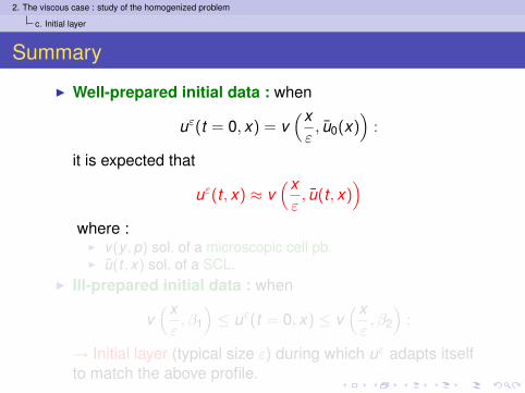
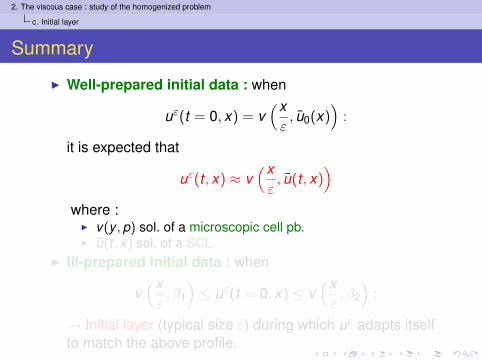
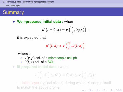
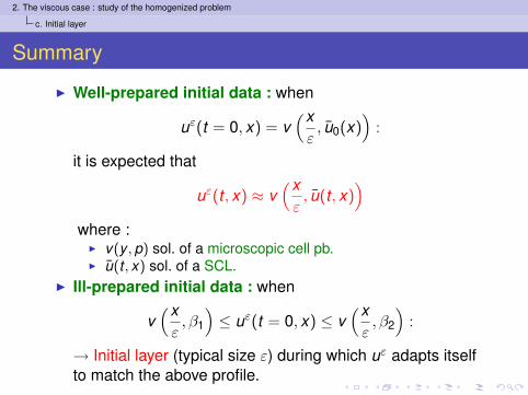
Summary
I Well-prepared initial data : when
uε(t = 0, x) = v(xε, u0(x)
):
it is expected that
uε(t , x) ≈ v(xε, u(t , x)
)where :
I v(y ,p) sol. of a microscopic cell pb.I u(t , x) sol. of a SCL.
I Ill-prepared initial data : when
v(xε, β1
)≤ uε(t = 0, x) ≤ v
(xε, β2
):
→ Initial layer (typical size ε) during which uε adapts itselfto match the above profile.
2. The viscous case : study of the homogenized problem
c. Initial layer
Summary
I Well-prepared initial data : when
uε(t = 0, x) = v(xε, u0(x)
):
it is expected that
uε(t , x) ≈ v(xε, u(t , x)
)where :
I v(y ,p) sol. of a microscopic cell pb.I u(t , x) sol. of a SCL.
I Ill-prepared initial data : when
v(xε, β1
)≤ uε(t = 0, x) ≤ v
(xε, β2
):
→ Initial layer (typical size ε) during which uε adapts itselfto match the above profile.
3. The viscous case : convergence proof
Outline
1. Introduction
2. The viscous case : study of the homogenized problem
3. The viscous case : convergence proofa. Main resultb. Kinetic formulationc. Passing to the limit - Well-prepared cased. Ill-prepared case
4. The hyperbolic case
3. The viscous case : convergence proof
a. Main result
Outline
1. Introduction
2. The viscous case : study of the homogenized problem
3. The viscous case : convergence proofa. Main resultb. Kinetic formulationc. Passing to the limit - Well-prepared cased. Ill-prepared case
4. The hyperbolic case
3. The viscous case : convergence proof
a. Main result
Main result
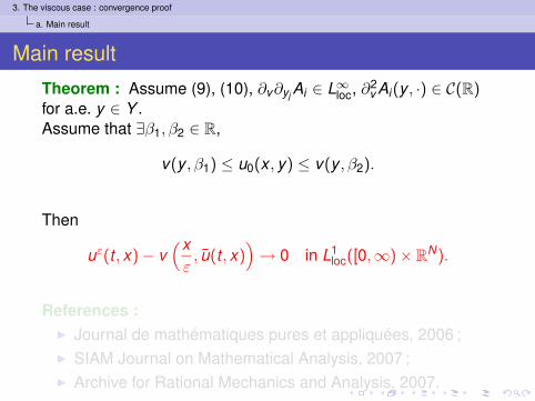
Theorem : Assume (9), (10), ∂v∂yj Ai ∈ L∞loc, ∂2v Ai(y , ·) ∈ C(R)
for a.e. y ∈ Y .Assume that ∃β1, β2 ∈ R,
v(y , β1) ≤ u0(x , y) ≤ v(y , β2).
Then
uε(t , x)− v(xε, u(t , x)
)→ 0 in L1
loc([0,∞)× RN).
References :I Journal de mathématiques pures et appliquées, 2006 ;I SIAM Journal on Mathematical Analysis, 2007 ;I Archive for Rational Mechanics and Analysis, 2007.

3. The viscous case : convergence proof
a. Main result
Main result
Theorem : Assume (9), (10), ∂v∂yj Ai ∈ L∞loc, ∂2v Ai(y , ·) ∈ C(R)
for a.e. y ∈ Y .Assume that ∃β1, β2 ∈ R,
v(y , β1) ≤ u0(x , y) ≤ v(y , β2).
Then
uε(t , x)− v(xε, u(t , x)
)→ 0 in L1
loc([0,∞)× RN).
References :I Journal de mathématiques pures et appliquées, 2006 ;I SIAM Journal on Mathematical Analysis, 2007 ;I Archive for Rational Mechanics and Analysis, 2007.
3. The viscous case : convergence proof
b. Kinetic formulation
Outline
1. Introduction
2. The viscous case : study of the homogenized problem
3. The viscous case : convergence proofa. Main resultb. Kinetic formulationc. Passing to the limit - Well-prepared cased. Ill-prepared case
4. The hyperbolic case
3. The viscous case : convergence proof
b. Kinetic formulation
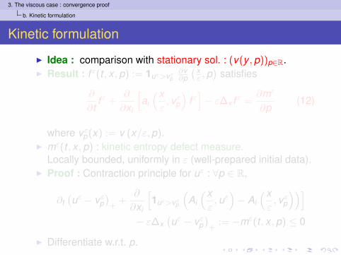
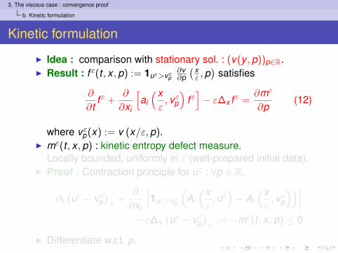
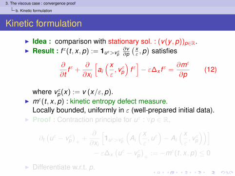
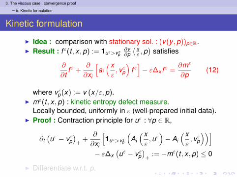
Kinetic formulation
I Idea : comparison with stationary sol. : (v(y ,p))p∈R.I Result : f ε(t , x ,p) := 1uε>vε
p∂v∂p
( xε ,p
)satisfies
∂
∂tf ε +
∂
∂xi
[ai
(xε, vε
p
)f ε
]− ε∆x f ε =
∂mε
∂p(12)
where vεp(x) := v (x/ε,p).
I mε(t , x ,p) : kinetic entropy defect measure.Locally bounded, uniformly in ε (well-prepared initial data).
I Proof : Contraction principle for uε : ∀p ∈ R,
∂t(uε − vε
p)+
+∂
∂xi
[1uε>vε
p
(Ai
(xε,uε
)− Ai
(xε, vε
p
))]− ε∆x
(uε − vε
p)+
:= −mε(t , x ,p) ≤ 0
I Differentiate w.r.t. p.
3. The viscous case : convergence proof
b. Kinetic formulation
Kinetic formulation
I Idea : comparison with stationary sol. : (v(y ,p))p∈R.I Result : f ε(t , x ,p) := 1uε>vε
p∂v∂p
( xε ,p
)satisfies
∂
∂tf ε +
∂
∂xi
[ai
(xε, vε
p
)f ε
]− ε∆x f ε =
∂mε
∂p(12)
where vεp(x) := v (x/ε,p).
I mε(t , x ,p) : kinetic entropy defect measure.Locally bounded, uniformly in ε (well-prepared initial data).
I Proof : Contraction principle for uε : ∀p ∈ R,
∂t(uε − vε
p)+
+∂
∂xi
[1uε>vε
p
(Ai
(xε,uε
)− Ai
(xε, vε
p
))]− ε∆x
(uε − vε
p)+
:= −mε(t , x ,p) ≤ 0
I Differentiate w.r.t. p.
3. The viscous case : convergence proof
c. Passing to the limit - Well-prepared case
Outline
1. Introduction
2. The viscous case : study of the homogenized problem
3. The viscous case : convergence proofa. Main resultb. Kinetic formulationc. Passing to the limit - Well-prepared cased. Ill-prepared case
4. The hyperbolic case
3. The viscous case : convergence proof
c. Passing to the limit - Well-prepared case
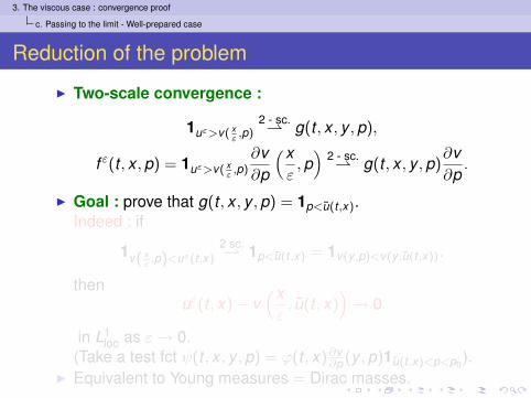
Reduction of the problem
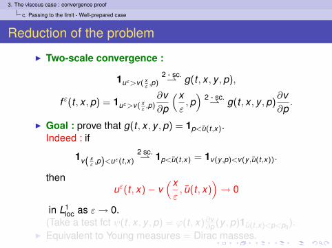
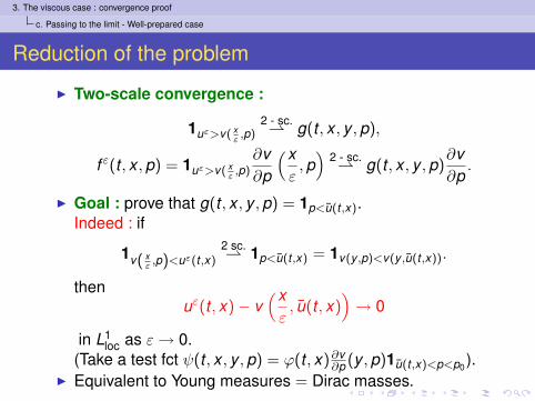
I Two-scale convergence :
1uε>v( xε,p)
2 - sc.⇀ g(t , x , y ,p),
f ε(t , x ,p) = 1uε>v( xε,p)
∂v∂p
(xε,p
)2 - sc.⇀ g(t , x , y ,p)
∂v∂p.
I Goal : prove that g(t , x , y ,p) = 1p<u(t ,x).Indeed : if
1v( xε,p)<uε(t ,x)
2 sc.⇀ 1p<u(t ,x) = 1v(y ,p)<v(y ,u(t ,x)).
thenuε(t , x)− v
(xε, u(t , x)
)→ 0
in L1loc as ε→ 0.
(Take a test fct ψ(t , x , y ,p) = ϕ(t , x)∂v∂p (y ,p)1u(t ,x)<p<p0
).I Equivalent to Young measures = Dirac masses.
3. The viscous case : convergence proof
c. Passing to the limit - Well-prepared case
Reduction of the problem
I Two-scale convergence :
1uε>v( xε,p)
2 - sc.⇀ g(t , x , y ,p),
f ε(t , x ,p) = 1uε>v( xε,p)
∂v∂p
(xε,p
)2 - sc.⇀ g(t , x , y ,p)
∂v∂p.
I Goal : prove that g(t , x , y ,p) = 1p<u(t ,x).Indeed : if
1v( xε,p)<uε(t ,x)
2 sc.⇀ 1p<u(t ,x) = 1v(y ,p)<v(y ,u(t ,x)).
thenuε(t , x)− v
(xε, u(t , x)
)→ 0
in L1loc as ε→ 0.
(Take a test fct ψ(t , x , y ,p) = ϕ(t , x)∂v∂p (y ,p)1u(t ,x)<p<p0
).I Equivalent to Young measures = Dirac masses.
3. The viscous case : convergence proof
c. Passing to the limit - Well-prepared case
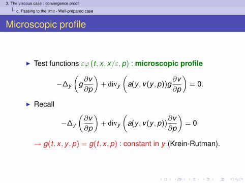
Microscopic profile
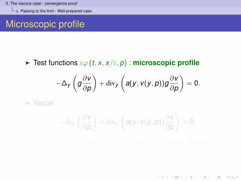
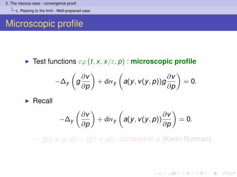
I Test functions εϕ (t , x , x/ε, p) : microscopic profile
−∆y
(g∂v∂p
)+ divy
(a(y , v(y ,p))g
∂v∂p
)= 0.
I Recall
−∆y
(∂v∂p
)+ divy
(a(y , v(y ,p))
∂v∂p
)= 0.
→ g(t , x , y ,p) = g(t , x ,p) : constant in y (Krein-Rutman).
3. The viscous case : convergence proof
c. Passing to the limit - Well-prepared case
Microscopic profile
I Test functions εϕ (t , x , x/ε, p) : microscopic profile
−∆y
(g∂v∂p
)+ divy
(a(y , v(y ,p))g
∂v∂p
)= 0.
I Recall
−∆y
(∂v∂p
)+ divy
(a(y , v(y ,p))
∂v∂p
)= 0.
→ g(t , x , y ,p) = g(t , x ,p) : constant in y (Krein-Rutman).

3. The viscous case : convergence proof
c. Passing to the limit - Well-prepared case
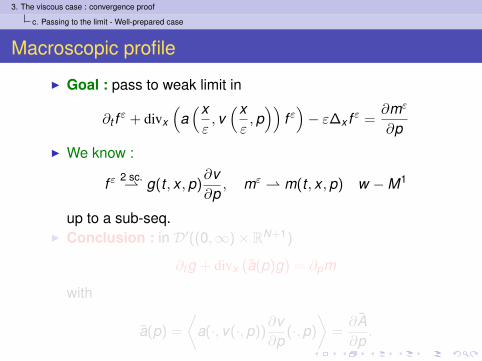
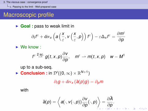
Macroscopic profile
I Goal : pass to weak limit in
∂t f ε + divx
(a
(xε, v
(xε,p
))f ε
)− ε∆x f ε =
∂mε
∂p
I We know :
f ε 2 sc.⇀ g(t , x ,p)
∂v∂p, mε ⇀ m(t , x ,p) w −M1
up to a sub-seq.I Conclusion : in D′((0,∞)× RN+1)
∂tg + divx (a(p)g) = ∂pm
with
a(p) =
⟨a(·, v(·,p))
∂v∂p
(·,p)
⟩=∂A∂p
.
3. The viscous case : convergence proof
c. Passing to the limit - Well-prepared case
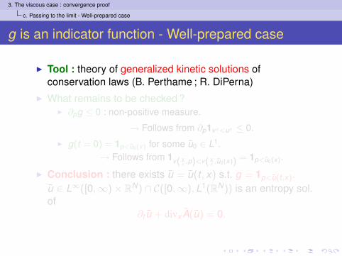
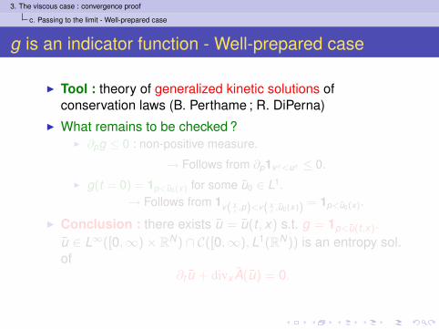
g is an indicator function - Well-prepared case
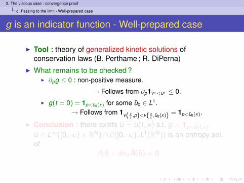
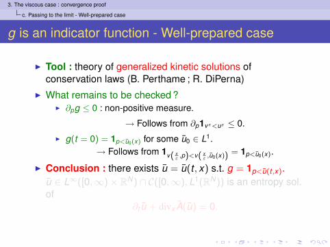
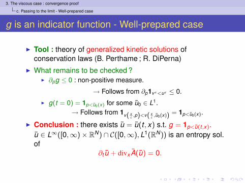
I Tool : theory of generalized kinetic solutions ofconservation laws (B. Perthame ; R. DiPerna)
I What remains to be checked ?I ∂pg ≤ 0 : non-positive measure.
→ Follows from ∂p1vε<uε ≤ 0.
I g(t = 0) = 1p<u0(x) for some u0 ∈ L1.→ Follows from 1v( x
ε ,p)<v( xε ,u0(x)) = 1p<u0(x).
I Conclusion : there exists u = u(t , x) s.t. g = 1p<u(t ,x).u ∈ L∞([0,∞)× RN) ∩ C([0,∞),L1(RN)) is an entropy sol.of
∂t u + divx A(u) = 0.
3. The viscous case : convergence proof
c. Passing to the limit - Well-prepared case
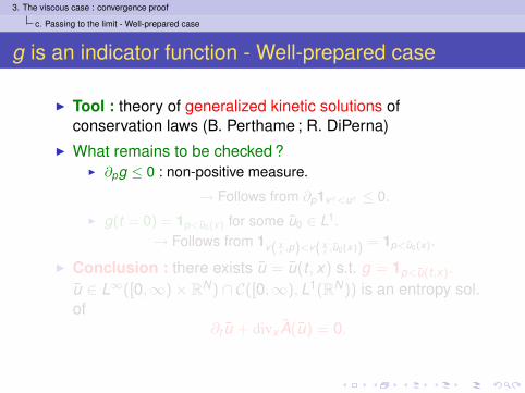
g is an indicator function - Well-prepared case
I Tool : theory of generalized kinetic solutions ofconservation laws (B. Perthame ; R. DiPerna)
I What remains to be checked ?I ∂pg ≤ 0 : non-positive measure.
→ Follows from ∂p1vε<uε ≤ 0.
I g(t = 0) = 1p<u0(x) for some u0 ∈ L1.→ Follows from 1v( x
ε ,p)<v( xε ,u0(x)) = 1p<u0(x).
I Conclusion : there exists u = u(t , x) s.t. g = 1p<u(t ,x).u ∈ L∞([0,∞)× RN) ∩ C([0,∞),L1(RN)) is an entropy sol.of
∂t u + divx A(u) = 0.
3. The viscous case : convergence proof
c. Passing to the limit - Well-prepared case
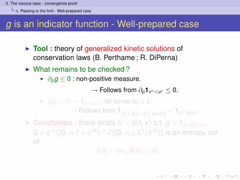
g is an indicator function - Well-prepared case
I Tool : theory of generalized kinetic solutions ofconservation laws (B. Perthame ; R. DiPerna)
I What remains to be checked ?I ∂pg ≤ 0 : non-positive measure.
→ Follows from ∂p1vε<uε ≤ 0.
I g(t = 0) = 1p<u0(x) for some u0 ∈ L1.→ Follows from 1v( x
ε ,p)<v( xε ,u0(x)) = 1p<u0(x).
I Conclusion : there exists u = u(t , x) s.t. g = 1p<u(t ,x).u ∈ L∞([0,∞)× RN) ∩ C([0,∞),L1(RN)) is an entropy sol.of
∂t u + divx A(u) = 0.
3. The viscous case : convergence proof
c. Passing to the limit - Well-prepared case
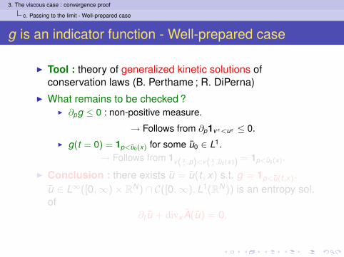
g is an indicator function - Well-prepared case
I Tool : theory of generalized kinetic solutions ofconservation laws (B. Perthame ; R. DiPerna)
I What remains to be checked ?I ∂pg ≤ 0 : non-positive measure.
→ Follows from ∂p1vε<uε ≤ 0.
I g(t = 0) = 1p<u0(x) for some u0 ∈ L1.→ Follows from 1v( x
ε ,p)<v( xε ,u0(x)) = 1p<u0(x).
I Conclusion : there exists u = u(t , x) s.t. g = 1p<u(t ,x).u ∈ L∞([0,∞)× RN) ∩ C([0,∞),L1(RN)) is an entropy sol.of
∂t u + divx A(u) = 0.
3. The viscous case : convergence proof
c. Passing to the limit - Well-prepared case
g is an indicator function - Well-prepared case
I Tool : theory of generalized kinetic solutions ofconservation laws (B. Perthame ; R. DiPerna)
I What remains to be checked ?I ∂pg ≤ 0 : non-positive measure.
→ Follows from ∂p1vε<uε ≤ 0.
I g(t = 0) = 1p<u0(x) for some u0 ∈ L1.→ Follows from 1v( x
ε ,p)<v( xε ,u0(x)) = 1p<u0(x).
I Conclusion : there exists u = u(t , x) s.t. g = 1p<u(t ,x).u ∈ L∞([0,∞)× RN) ∩ C([0,∞),L1(RN)) is an entropy sol.of
∂t u + divx A(u) = 0.
3. The viscous case : convergence proof
d. Ill-prepared case
Outline
1. Introduction
2. The viscous case : study of the homogenized problem
3. The viscous case : convergence proofa. Main resultb. Kinetic formulationc. Passing to the limit - Well-prepared cased. Ill-prepared case
4. The hyperbolic case
3. The viscous case : convergence proof
d. Ill-prepared case
Ill-prepared case
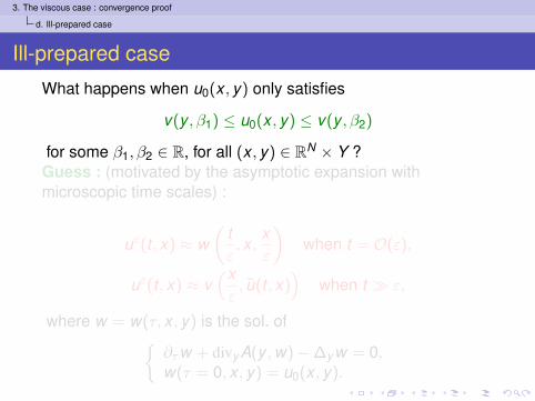
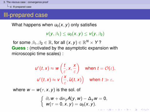
What happens when u0(x , y) only satisfies
v(y , β1) ≤ u0(x , y) ≤ v(y , β2)
for some β1, β2 ∈ R, for all (x , y) ∈ RN × Y ?Guess : (motivated by the asymptotic expansion withmicroscopic time scales) :
uε(t , x) ≈ w(
tε, x ,
xε
)when t = O(ε),
uε(t , x) ≈ v(xε, u(t , x)
)when t � ε,
where w = w(τ, x , y) is the sol. of{∂τw + divyA(y ,w)−∆yw = 0,w(τ = 0, x , y) = u0(x , y).
3. The viscous case : convergence proof
d. Ill-prepared case
Ill-prepared case
What happens when u0(x , y) only satisfies
v(y , β1) ≤ u0(x , y) ≤ v(y , β2)
for some β1, β2 ∈ R, for all (x , y) ∈ RN × Y ?Guess : (motivated by the asymptotic expansion withmicroscopic time scales) :
uε(t , x) ≈ w(
tε, x ,
xε
)when t = O(ε),
uε(t , x) ≈ v(xε, u(t , x)
)when t � ε,
where w = w(τ, x , y) is the sol. of{∂τw + divyA(y ,w)−∆yw = 0,w(τ = 0, x , y) = u0(x , y).
3. The viscous case : convergence proof
d. Ill-prepared case
Ill-prepared caseSketch of proof
Proof follows asymptotic expansion. Ingredients are
1. L1 contraction principle ;2. Result in case of well-prepared initial data ;3. Exponential convergence of w towards v(y , u0(x)).
OP : What if the hypothesis on the initial data is not satisfied ?
4. The hyperbolic case
Outline
1. Introduction
2. The viscous case : study of the homogenized problem
3. The viscous case : convergence proof
4. The hyperbolic casea. Setting of the problemb. Focus on the divergence free casec. The general case
4. The hyperbolic case
a. Setting of the problem
Outline
1. Introduction
2. The viscous case : study of the homogenized problem
3. The viscous case : convergence proof
4. The hyperbolic casea. Setting of the problemb. Focus on the divergence free casec. The general case

4. The hyperbolic case
a. Setting of the problem
Setting of the problem
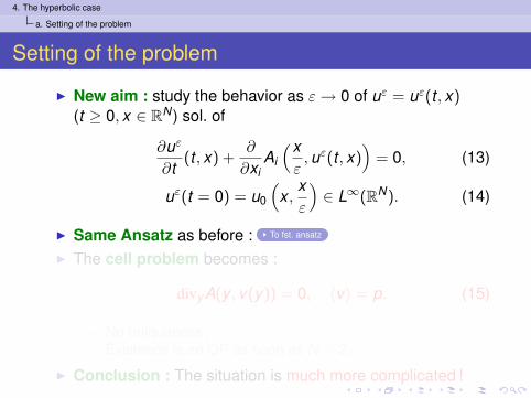
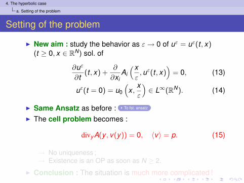
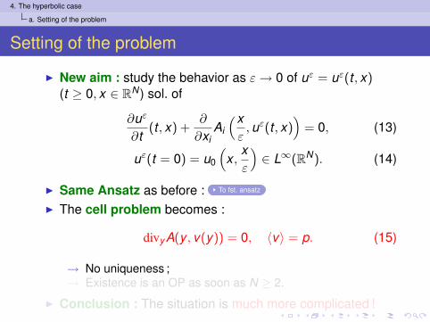
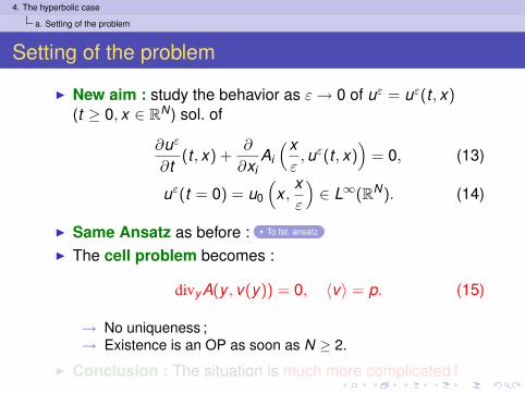
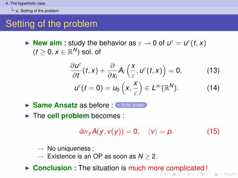
I New aim : study the behavior as ε→ 0 of uε = uε(t , x)(t ≥ 0, x ∈ RN ) sol. of
∂uε
∂t(t , x) +
∂
∂xiAi
(xε,uε(t , x)
)= 0, (13)
uε(t = 0) = u0
(x ,
xε
)∈ L∞(RN). (14)
I Same Ansatz as before :I The cell problem becomes :
divyA(y , v(y)) = 0, 〈v〉 = p. (15)
→ No uniqueness ;→ Existence is an OP as soon as N ≥ 2.
I Conclusion : The situation is much more complicated !
4. The hyperbolic case
a. Setting of the problem
Setting of the problem
I New aim : study the behavior as ε→ 0 of uε = uε(t , x)(t ≥ 0, x ∈ RN ) sol. of
∂uε
∂t(t , x) +
∂
∂xiAi
(xε,uε(t , x)
)= 0, (13)
uε(t = 0) = u0
(x ,
xε
)∈ L∞(RN). (14)
I Same Ansatz as before : To fst. ansatz
I The cell problem becomes :
divyA(y , v(y)) = 0, 〈v〉 = p. (15)
→ No uniqueness ;→ Existence is an OP as soon as N ≥ 2.
I Conclusion : The situation is much more complicated !

4. The hyperbolic case
a. Setting of the problem
Former results
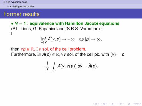
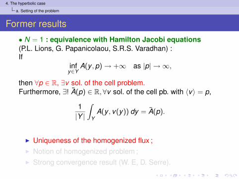
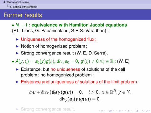
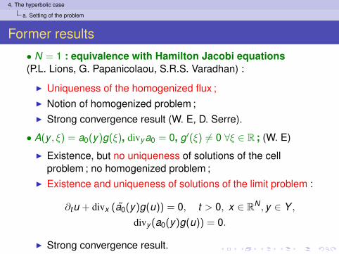
• N = 1 : equivalence with Hamilton Jacobi equations(P.L. Lions, G. Papanicolaou, S.R.S. Varadhan) :
4. The hyperbolic case
a. Setting of the problem
Former results
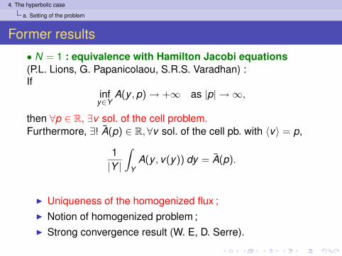
• N = 1 : equivalence with Hamilton Jacobi equations(P.L. Lions, G. Papanicolaou, S.R.S. Varadhan) :If
infy∈Y
A(y ,p) → +∞ as |p| → ∞,
then ∀p ∈ R, ∃v sol. of the cell problem.Furthermore, ∃! A(p) ∈ R,∀v sol. of the cell pb. with 〈v〉 = p,
1|Y |
∫Y
A(y , v(y)) dy = A(p).
4. The hyperbolic case
a. Setting of the problem
Former results
• N = 1 : equivalence with Hamilton Jacobi equations(P.L. Lions, G. Papanicolaou, S.R.S. Varadhan) :If
infy∈Y
A(y ,p) → +∞ as |p| → ∞,
then ∀p ∈ R, ∃v sol. of the cell problem.Furthermore, ∃! A(p) ∈ R,∀v sol. of the cell pb. with 〈v〉 = p,
1|Y |
∫Y
A(y , v(y)) dy = A(p).
I Uniqueness of the homogenized flux ;I Notion of homogenized problem ;I Strong convergence result (W. E, D. Serre).
4. The hyperbolic case
a. Setting of the problem
Former results
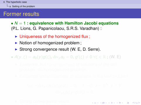
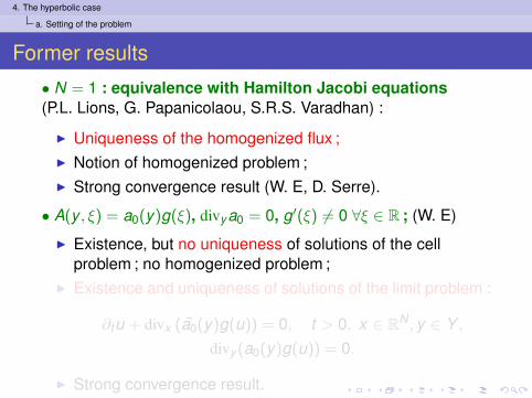
• N = 1 : equivalence with Hamilton Jacobi equations(P.L. Lions, G. Papanicolaou, S.R.S. Varadhan) :
I Uniqueness of the homogenized flux ;I Notion of homogenized problem ;I Strong convergence result (W. E, D. Serre).
• A(y , ξ) = a0(y)g(ξ), divya0 = 0, g′(ξ) 6= 0 ∀ξ ∈ R ; (W. E)
I Existence, but no uniqueness of solutions of the cellproblem ; no homogenized problem ;
I Existence and uniqueness of solutions of the limit problem :
∂tu + divx (a0(y)g(u)) = 0, t > 0, x ∈ RN , y ∈ Y ,divy (a0(y)g(u)) = 0.
I Strong convergence result.

4. The hyperbolic case
a. Setting of the problem
Former results
• N = 1 : equivalence with Hamilton Jacobi equations(P.L. Lions, G. Papanicolaou, S.R.S. Varadhan) :
I Uniqueness of the homogenized flux ;I Notion of homogenized problem ;I Strong convergence result (W. E, D. Serre).
• A(y , ξ) = a0(y)g(ξ), divya0 = 0, g′(ξ) 6= 0 ∀ξ ∈ R ; (W. E)
I Existence, but no uniqueness of solutions of the cellproblem ; no homogenized problem ;
I Existence and uniqueness of solutions of the limit problem :
∂tu + divx (a0(y)g(u)) = 0, t > 0, x ∈ RN , y ∈ Y ,divy (a0(y)g(u)) = 0.
I Strong convergence result.
4. The hyperbolic case
b. Focus on the divergence free case
Outline
1. Introduction
2. The viscous case : study of the homogenized problem
3. The viscous case : convergence proof
4. The hyperbolic casea. Setting of the problemb. Focus on the divergence free casec. The general case
4. The hyperbolic case
b. Focus on the divergence free case
Microscopic constraints
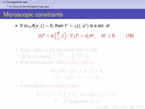
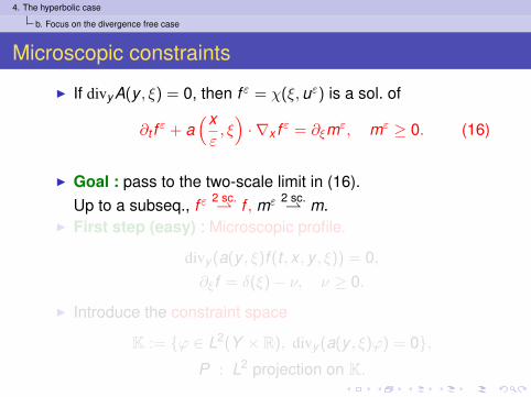
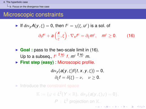
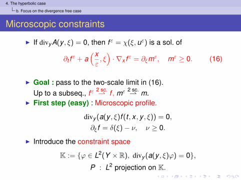
I If divyA(y , ξ) = 0, then f ε = χ(ξ,uε) is a sol. of
∂t f ε + a(xε, ξ
)· ∇x f ε = ∂ξmε, mε ≥ 0. (16)
I Goal : pass to the two-scale limit in (16).Up to a subseq., f ε 2 sc.
⇀ f , mε 2 sc.⇀ m.
I First step (easy) : Microscopic profile.
divy (a(y , ξ)f (t , x , y , ξ)) = 0,∂ξf = δ(ξ)− ν, ν ≥ 0.
I Introduce the constraint space
K := {ϕ ∈ L2(Y × R), divy (a(y , ξ)ϕ) = 0},P : L2 projection on K.
4. The hyperbolic case
b. Focus on the divergence free case
Microscopic constraints
I If divyA(y , ξ) = 0, then f ε = χ(ξ,uε) is a sol. of
∂t f ε + a(xε, ξ
)· ∇x f ε = ∂ξmε, mε ≥ 0. (16)
I Goal : pass to the two-scale limit in (16).Up to a subseq., f ε 2 sc.
⇀ f , mε 2 sc.⇀ m.
I First step (easy) : Microscopic profile.
divy (a(y , ξ)f (t , x , y , ξ)) = 0,∂ξf = δ(ξ)− ν, ν ≥ 0.
I Introduce the constraint space
K := {ϕ ∈ L2(Y × R), divy (a(y , ξ)ϕ) = 0},P : L2 projection on K.
4. The hyperbolic case
b. Focus on the divergence free case
(Formal) macroscopic evolution equation
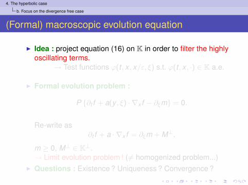
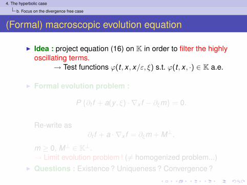
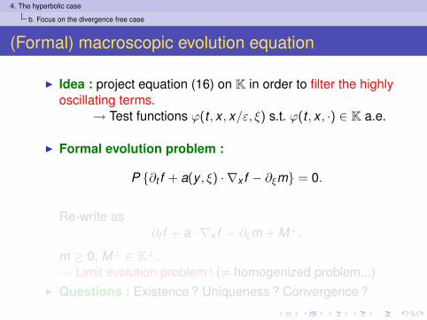
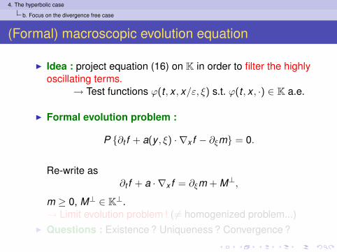
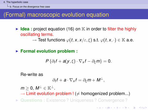
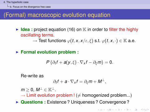
I Idea : project equation (16) on K in order to filter the highlyoscillating terms.
→ Test functions ϕ(t , x , x/ε, ξ) s.t. ϕ(t , x , ·) ∈ K a.e.
I Formal evolution problem :
P {∂t f + a(y , ξ) · ∇x f − ∂ξm} = 0.
Re-write as∂t f + a · ∇x f = ∂ξm + M⊥,
m ≥ 0, M⊥ ∈ K⊥.→ Limit evolution problem ! ( 6= homogenized problem...)
I Questions : Existence ? Uniqueness ? Convergence ?
4. The hyperbolic case
b. Focus on the divergence free case
(Formal) macroscopic evolution equation
I Idea : project equation (16) on K in order to filter the highlyoscillating terms.
→ Test functions ϕ(t , x , x/ε, ξ) s.t. ϕ(t , x , ·) ∈ K a.e.
I Formal evolution problem :
P {∂t f + a(y , ξ) · ∇x f − ∂ξm} = 0.
Re-write as∂t f + a · ∇x f = ∂ξm + M⊥,
m ≥ 0, M⊥ ∈ K⊥.→ Limit evolution problem ! ( 6= homogenized problem...)
I Questions : Existence ? Uniqueness ? Convergence ?
4. The hyperbolic case
b. Focus on the divergence free case
Rigorous result
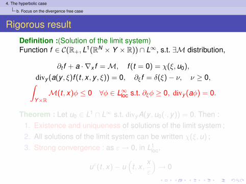
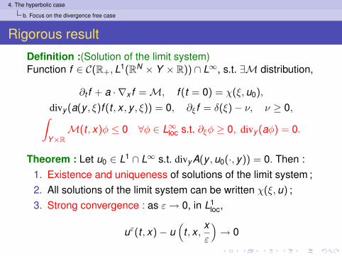
Definition :(Solution of the limit system)Function f ∈ C(R+,L1(RN × Y × R)) ∩ L∞, s.t. ∃M distribution,
∂t f + a · ∇x f = M, f (t = 0) = χ(ξ,u0),
divy (a(y , ξ)f (t , x , y , ξ)) = 0, ∂ξf = δ(ξ)− ν, ν ≥ 0,∫Y×R
M(t , x)φ ≤ 0 ∀φ ∈ L∞loc s.t. ∂ξφ ≥ 0, divy (aφ) = 0.
Theorem : Let u0 ∈ L1 ∩ L∞ s.t. divyA(y ,u0(·, y)) = 0. Then :1. Existence and uniqueness of solutions of the limit system ;2. All solutions of the limit system can be written χ(ξ, u) ;3. Strong convergence : as ε→ 0, in L1
loc,
uε(t , x)− u(
t , x ,xε
)→ 0
4. The hyperbolic case
b. Focus on the divergence free case
Rigorous result
Definition :(Solution of the limit system)Function f ∈ C(R+,L1(RN × Y × R)) ∩ L∞, s.t. ∃M distribution,
∂t f + a · ∇x f = M, f (t = 0) = χ(ξ,u0),
divy (a(y , ξ)f (t , x , y , ξ)) = 0, ∂ξf = δ(ξ)− ν, ν ≥ 0,∫Y×R
M(t , x)φ ≤ 0 ∀φ ∈ L∞loc s.t. ∂ξφ ≥ 0, divy (aφ) = 0.
Theorem : Let u0 ∈ L1 ∩ L∞ s.t. divyA(y ,u0(·, y)) = 0. Then :1. Existence and uniqueness of solutions of the limit system ;2. All solutions of the limit system can be written χ(ξ, u) ;3. Strong convergence : as ε→ 0, in L1
loc,
uε(t , x)− u(
t , x ,xε
)→ 0
4. The hyperbolic case
c. The general case
Outline
1. Introduction
2. The viscous case : study of the homogenized problem
3. The viscous case : convergence proof
4. The hyperbolic casea. Setting of the problemb. Focus on the divergence free casec. The general case
4. The hyperbolic case
c. The general case
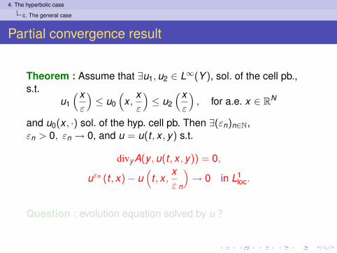
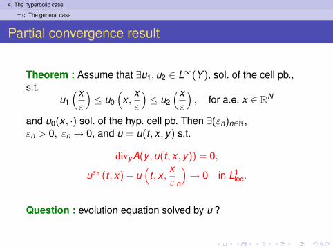
Partial convergence result
Theorem : Assume that ∃u1,u2 ∈ L∞(Y ), sol. of the cell pb.,s.t.
u1
(xε
)≤ u0
(x ,
xε
)≤ u2
(xε
), for a.e. x ∈ RN
and u0(x , ·) sol. of the hyp. cell pb. Then ∃(εn)n∈N,εn > 0, εn → 0, and u = u(t , x , y) s.t.
divyA(y ,u(t , x , y)) = 0,
uεn (t , x)− u(
t , x ,xε n
)→ 0 in L1
loc.
Question : evolution equation solved by u ?
4. The hyperbolic case
c. The general case
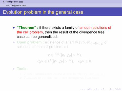
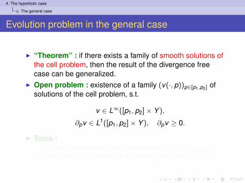
Evolution problem in the general case
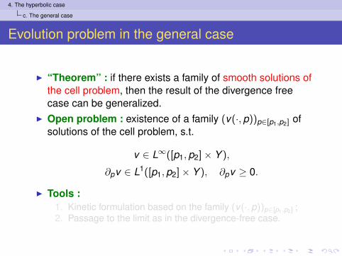
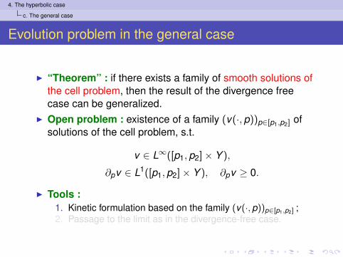
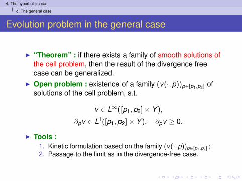
I “Theorem” : if there exists a family of smooth solutions ofthe cell problem, then the result of the divergence freecase can be generalized.
I Open problem : existence of a family (v(·,p))p∈[p1,p2] ofsolutions of the cell problem, s.t.
v ∈ L∞([p1,p2]× Y ),
∂pv ∈ L1([p1,p2]× Y ), ∂pv ≥ 0.
I Tools :1. Kinetic formulation based on the family (v(·,p))p∈[p1,p2] ;2. Passage to the limit as in the divergence-free case.
4. The hyperbolic case
c. The general case
Evolution problem in the general case
I “Theorem” : if there exists a family of smooth solutions ofthe cell problem, then the result of the divergence freecase can be generalized.
I Open problem : existence of a family (v(·,p))p∈[p1,p2] ofsolutions of the cell problem, s.t.
v ∈ L∞([p1,p2]× Y ),
∂pv ∈ L1([p1,p2]× Y ), ∂pv ≥ 0.
I Tools :1. Kinetic formulation based on the family (v(·,p))p∈[p1,p2] ;2. Passage to the limit as in the divergence-free case.
ConclusionOpen problems and other directions
Case with vanishing viscosity :
I More thorough existence theory for the elliptic cellproblem ;
I Hypothesis on the initial data in the ill-prepared case (is L∞
enough ?)
Case without viscosity :
I Existence of solutions of the cell problem (non-divergencefree case) ;
I Case when the initial data is ill-prepared ? (nonlinearityassumptions on the flux...)
Recommended


![Homogénéisation d’un réseau de poutres baignant da[] · considérées : s0 (déplacement des poutres) et 0 (potentiel de déplacements du fluide). Sous forme Sous forme variationnelle,](https://img.pdfslide.tips/doc/110x75/5b9cea9709d3f272468d8ddd/homogeneisation-dun-reseau-de-poutres-baignant-da-considerees-s0.jpg)
![Predgovor - imft.ftn.uns.ac.rsimft.ftn.uns.ac.rs/~ljubo/Nauka/Mg.pdf · Savremenu teoriju LDP su uobliˇcili S.R.S. Varadhan, Donsker, Freidlin i Wentzell (vidi [DeZe98], [DeSt98],](https://img.pdfslide.tips/doc/110x75/5e07e16bc2bfda5d5a17e41c/predgovor-imftftnunsac-ljubonaukamgpdf-savremenu-teoriju-ldp-su-uoblicili.jpg)