Embed Size (px)
Citation preview
Master APE September 2014
Long-‐term contracts and entry deterrence in the French electricity market
Author: REID, Christopher Supervisor: SPECTOR, David Referee: TROPEANO, Jean-‐Philippe
JEL codes: D43, L94 Keywords: Electricity, contracts, market entry, simulation
1
Abstract
Motivated by recent EU case law, we investigate how long-‐term contracts may be used as a
means of entry deterrence in the French electricity market. In our model this market consists of
two segments: a conventional (e.g. gas, coal) segment in which there is perfect competition, and
a nuclear segment dominated by one producer. Our analysis is focused on market entry in the
nuclear segment. The nuclear capacity that maximises the monopoly profit also minimizes the
total cost of electricity production. Thus, the monopoly capacity is efficient. When there is
market entry, firms compete via a discriminatory auction mechanism. We simulate the model,
calibrated to the French electricity market. In the absence of contracts, market entry leads to
excess capacity: the total cost of electricity production increases, while total profit and the price
of electricity decrease. Long-‐term contracts lead to reduced entry, but cannot eliminate entry
unless the rival has large fixed costs. Using contracts, the incumbent can increase its profit
compared to free entry, but cannot recover the monopoly profit. The price of electricity on the
spot market is not significantly affected by long-‐term contracts. Overall, the welfare effect of
long-‐term contracts is ambiguous.
2
Table of Contents
Abstract .............................................................................................................................................. 1
Introduction ..................................................................................................................................... 3
1. Literature review .................................................................................................................... 5
2. Monopoly: optimal capacity ................................................................................................ 8
2.1. Electricity demand ....................................................................................................................... 8
2.2. Efficient capacity level ............................................................................................................. 10
2.3. Nuclear capacity under monopoly ....................................................................................... 12
3. Duopoly: optimal capacity and contracts .................................................................... 14
3.1. Auction mechanism ................................................................................................................... 14
3.2. Large firm profit and optimal capacity ............................................................................... 17
3.3. Small firm profit and optimal capacity ............................................................................... 18
3.4. Long-‐term contracts .................................................................................................................. 19
4. Numerical simulation ......................................................................................................... 22
4.1. Calibration .................................................................................................................................... 22
4.2. Monopoly ...................................................................................................................................... 22
4.3. Duopoly ......................................................................................................................................... 23
4.4. Long-‐term contracts .................................................................................................................. 25
Conclusion ...................................................................................................................................... 29
References ..................................................................................................................................... 31
Appendix – selected MATLAB code ........................................................................................ 32
3
Introduction
On 17 March 2010, the European Commission (EC) adopted a decision1 concerning the
French market for the supply of electricity to large industrial customers. The Commission was
concerned that EDF (the incumbent operator) may have abused its dominant position by
concluding long-‐term supply contracts which had the effect of foreclosing the market.
Aaccording to the Commission, the volume and duration of EDF’s contracts did not provide
sufficient opportunities for alternative suppliers to compete “for the contracts”. In addition, the
exclusionary nature of the contracts (whether through explicit provisions in the contract or de
facto exclusivity) may have restricted competition “during the contracts”. The contracts also
prohibited clients from reselling electricity, limiting customers’ ability to manage their
consumption.
In response to these objections, EDF proposed a set of commitments, which the
Commission made legally binding in its March 2010 decision. Firstly, 65% of the electricity
supplied to large industrial customers would return to the market each year. Secondly, the
duration of contracts without free opt-‐out would be limited to five years. Finally, EDF would
allow competition during the contract period by systematically proposing an alternative
supplier, enabling customers to source electricity simultaneously from two suppliers. EDF also
made a commitment to end restrictions on the resale of electricity by clients under contract.
This decision by the EC forms the motivation for our research. We investigate the impact
of long-‐term supply contracts in a simple model of the French electricity market. This market is
characterized by the fact that nuclear power stations constitute a large proportion of installed
generating capacity. Although in practice EDF must guarantee competitors access to low-‐cost
nuclear electricity, the nuclear capacity remains under the control of EDF, the incumbent
operator. We consider here that EDF has exclusive rights over its nuclear capacity, and we focus
our analysis on competition in this segment of the market.
Compared to coal and gas power stations where fuel costs are high, nuclear power has
low operating costs. However, the investment costs for nuclear are much higher and must be
accounted for throughout the lifetime of the power station. This feature of nuclear energy
makes market entry particularly difficult. We model the French electricity market as two
segments: a conventional (coal and gas) segment with high operating costs, and a nuclear
1 see press release IP/10/290 of 17 March 2010 and Bessot et al. (2010)
4
segment dominated by EDF. We consider that the conventional segment is perfectly
competitive: as a result of market entry, firms make zero profit in this segment. By contrast, the
nuclear segment is a monopoly: all installed capacity is controlled by EDF. In addition, EDF may
sign long-‐term supply contracts with large industrial customers. We study market entry in the
nuclear segment first in the absence of contracts, and then we introduce contracts to determine
whether they may be used to dissuade entry.
Our findings provide a theoretical basis for the EC’s decision: long-‐term contracts do
indeed have a foreclosure effect on the market, leading to reduced entry by potential rivals. In
the presence of large fixed costs or a minimum efficient scale, a sufficient volume of long-‐term
contracts may even exclude rivals. However, the welfare effect is ambiguous. The capacity
installed by the monopoly is optimal from the point of view of production efficiency. Hence,
market entry leads to excess capacity, increasing the cost of producing electricity. However,
market entry also leads to lower total profits for electricity suppliers and reduces the average
price of electricity. This decrease in price may be viewed as beneficial from the point of view of
consumers, although lower profits may lead to insufficient investment in the future (this time
dimension is absent from our model).
By decreasing excess entry, long-‐term contracts help to minimize the total cost of
producing electricity. Furthermore, their effect on spot market price is very limited (compared
to the spot market price after market entry, in the absence of contracts). However, customers
who have signed a long-‐term contract are committed to paying a high price for electricity and
cannot benefit from the reduced spot market price.
The paper is structured as follows: we begin by reviewing the literature on contracts as
a means of entry deterrence. In section two, we calculate the capacity that minimizes the total
cost of electricity production, and the capacity that maximizes monopoly profit. In section three,
we introduce a second producer and derive analytical expressions for the two firms’ profits and
capacity choices, with and without contracts. In section four, we simulate the model (calibrated
to the French electricity market) and discuss the results.
5
1. Literature review
Historically, exclusionary contracts have been a contentious issue in antitrust law and
scholarship. Rasmusen, Ramseyer and Wiley (1991) cite several cases in which US judges found
such contracts to be anticompetitive and illegal 1 . However, Chicago School academics
responded to such cases with scepticism. Director and Levi (1956) argued that customers
would not agree to sign exclusionary contracts with a company unless it offered them
compensation for lost customer surplus. Such compensation would exceed monopoly profits,
making exclusion too costly for the incumbent firm.
In a seminal paper, Aghion and Bolton (1987) show that exclusionary contracts may in
fact be used profitably for entry deterrence. In their model, two buyers agree to sign an
exclusionary agreement despite jointly preferring to refuse. The model depends on three
assumptions: first, the excluding firm can commit to a future price level, and each customer can
escape the contract by paying liquidated damages. Second, the entrant’s marginal cost is
unknown and may be different from the incumbent firm’s marginal cost, which is constant.
Third, active producers incur a fixed cost, leading to economies of scale. Aghion and Bolton also
allow the incumbent to make an offer to one buyer that is conditional on the other buyer’s
decision to accept the offer.
Rasmusen, Ramseyer, and Wiley (1991 – we refer to this paper as “RRW”) show that the
incumbent may exclude rivals by exploiting buyers’ lack of coordination, without requiring the
previous assumptions. Specifically, if there is a minimum efficient scale2, the incumbent need
only lock up a proportion of the customers to forestall entry. “If each customer believes that the
others will sign, each also believes that no rival seller will enter. Hence, a customer loses
nothing by signing the exclusionary agreement and will indeed sign.”
Segal and Whinston (2000) correct some errors in RRW and refine the analysis, focusing
on how an incumbent can use discriminatory offers to exploit externalities that exist among
buyers. The model has three periods, featuring three sets of agents: an incumbent firm, a
potential rival, and a set of buyers. In period one, the incumbent offers buyers exclusionary
contracts. In period two, the rival decides whether to enter, and in period three, active firms
compete à la Bertrand. The authors examine two different settings for period one:
1 Examples include: U.S. v. Aluminum Co. of America (1945), Lorain Journal Co. v. U.S. (1951), and United Shoe Machinery Corp. v. U.S. (1922). 2 RRW assume a minimum efficient scale, but no economies of scale beyond that. Hence, exclusion is not simply the result of a natural monopoly.
6
simultaneous offers and sequential offers. When the incumbent deals with buyers
simultaneously without the ability to discriminate, profitable exclusion relies on a lack of
coordination among buyers. This is not the case when the incumbent can discriminate between
buyers: discrimination allows the incumbent to exclude rivals profitably by exploiting
externalities across buyers. When the incumbent deals with buyers sequentially, its ability to
exclude is strengthened. Segal and Whinston show that when the number of buyers is large, the
incumbent is able to exclude for free.
A related literature deals with financial forward contracts. Unlike exclusionary
contracts, forward contracts do not forbid consumers from dealing with entrants and do not
directly restrict a producer’s choice of output and price. Instead of making legal restrictions,
they influence behaviour on the spot market by altering incentives for firms. Provided they are
observable, forward contracts may be used as a signal of commitment to future aggressive
behaviour on the spot market. In this way, they may have an entry deterrence effect similar to
that of exclusionary contracts. However, the effect is strongly dependent on whether firms
compete in quantity (Cournot competition) or price (Bertrand) on the spot market.
Allaz and Vila (1993) show that forward markets can improve the efficiency of
production decisions in a Cournot duopoly. They begin by noting that “usually appearance of
forward markets is justified by agents’ desire to hedge risk”, requiring uncertainty over some
variable. Allaz and Vila show that this is not necessary: forward markets can be used under
certainty and perfect foresight. Producers use forward transactions as strategic variables. The
authors first consider a two-‐period model of duopoly with linear costs and demand, under
perfect foresight and certainty. Firms choose forward positions in period one and produce in
period two. The firm with access to the forward market gains first-‐mover advantage (becomes
Stackelberg leader on the spot market). However, a prisoner’s dilemma arises when both firms
have access to the forward market: a firm greatly benefits from being the only producer to trade
forward, but if both firms trade forward, they end up worse off. The authors then extend the
model to trading periods, and show that when tends to infinity, the competitive
outcome is obtained.
Mahenc and Salanié (2004) investigate a model in which duopolists producing two
differentiated goods can trade forward before competing à la Bertrand on spot markets.
Similarly to Allaz-‐Vila, the model features two periods: in period one each firm takes a position
on the forward market, and in period two they compete on the spot market. However, the
crucial difference is that competition on the spot market is à la Bertrand: firms choose prices,
not quantities, and the goods are not perfect substitutes. Mahenc and Salanié reach a conclusion
that is opposite to that of Allaz and Vila: in equilibrium firms buy forward their own production,
leading to higher spot prices than in the static case (no forward market). Hence, forward
7
markets have a softening effect on competition in this case. This competition-‐softening effect is
stronger when competition increases, that is when goods are more substitutable.
Lien (2000) analyses the role of forward contracts in the electricity market. He argues
that there is a “curse of market power”: in the short term, large firms have an incentive to hold
back output in order to push up prices. However, this leads to excess entry by small producers,
who benefit from high prices without incurring the costs of restricted output. As a result, long-‐
term profits of large firms are reduced. Lien shows that forward sales can eliminate this curse
by deterring excess entry.
Our analysis differs from that of Lien in two important ways: firstly, we concentrate on
the French electricity market and in particular the nuclear segment of this market. The French
market is characterised by the high proportion of electricity that is provided by nuclear power
stations. Given the high investment costs associated with nuclear energy, entry is particularly
difficult in this segment of the market. Nuclear power stations typically provide baseload power
and are operational most of the time, which makes the use of long-‐term supply contracts
particularly convenient.
Secondly, we model competition in the electricity market using an auction mechanism
studied by Fabra, von der Fehr, and Harbord (2006). There are two producers in this model.
Each producer submits a bid (offer price) to a central auctioneer, who then allocates production
in order to meet demand. Fabra et al. study two mechanisms: a uniform auction, in which all
active producers (those whose bid is wholly or partly accepted) are paid the same price, and a
discriminatory auction, in which active producers are paid their offer price. The authors find
that uniform auctions result in higher prices than discriminatory auctions. In a related paper,
Fabra, von der Fehr, and de Frutos (2011) study the impact of the auction format on investment
incentives. They find that investment incentives are (weakly) stronger under discriminatory
auctions than under uniform auctions. For this reason, we focus on discriminatory auctions.
8
2. Monopoly: optimal capacity
In our model, the French electricity market consists of two segments: a perfectly
competitive conventional segment, and a nuclear segment dominated by one firm. Marginal
costs are constant: conventional electricity costs to produce, and nuclear electricity costs .
Operating costs for conventional generation are higher than for nuclear generation, so .
The conventional sector is perfectly competitive, so firms make zero profit. However,
the nuclear sector is run by a monopoly. Before considering entry by potential rivals in the
nuclear sector, we determine the optimal nuclear capacity from the point of view of social
welfare and from the monopoly’s point of view.
2.1. Electricity demand
In order to calculate optimal capacity, we need to characterise electricity demand.
Compared to demand in markets for goods, electricity demand is unusual. Firstly, demand is not
in terms of quantity but in terms of rate. Indeed, quantity is expressed in terms of energy, with
units of GWh (gigawatt-‐hour) for example, whereas demand and supply are expressed in terms
of power, with units of GW (gigawatt). This is because of a physical property of the system:
unlike goods, electricity cannot be stored. Hence, the rate at which electricity is provided to the
network must equal the rate at which it is consumed by customers. Secondly, it is almost
perfectly inelastic. That is, demand does not change in response to price.
The costs and given above are expressed in monetary units per quantity of
electricity, for example million euros per GWh (€m/GWh). However, this is equivalent to paying
for capacity for a certain time: if a firm supplies 10 GW for 2 hours at a cost of 0.03 €m/GWh, it
will incur a cost of € 600,000.
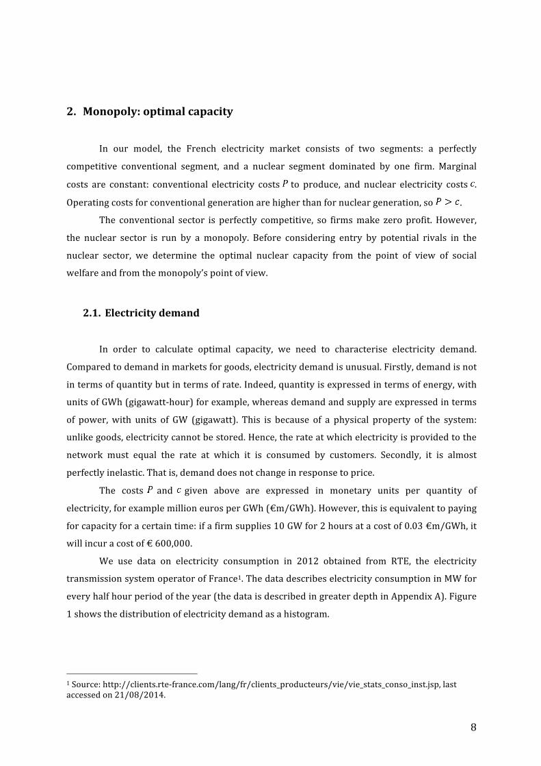
We use data on electricity consumption in 2012 obtained from RTE, the electricity
transmission system operator of France1. The data describes electricity consumption in MW for
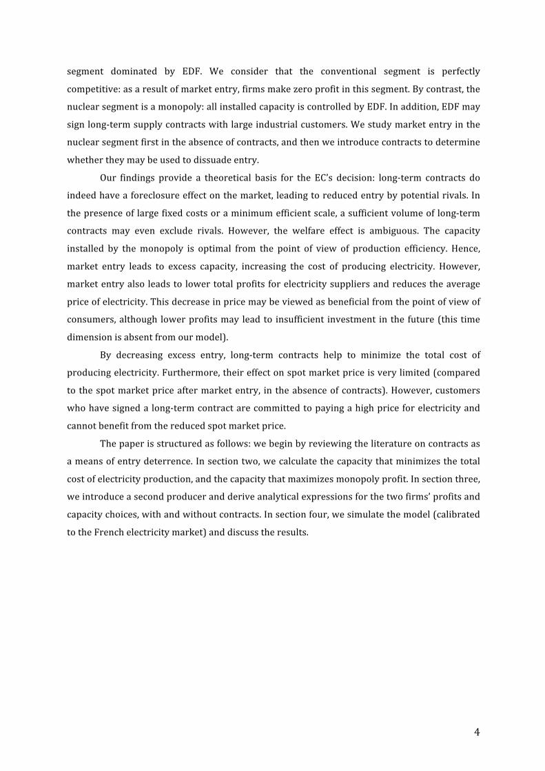
every half hour period of the year (the data is described in greater depth in Appendix A). Figure
1 shows the distribution of electricity demand as a histogram.
1 Source: http://clients.rte-‐france.com/lang/fr/clients_producteurs/vie/vie_stats_conso_inst.jsp, last accessed on 21/08/2014.
9
30 40 50 60 70 80 90 100 1100
10
20
30
40
50
60
70
Electricity demand (GW)
Freq
uenc
y (d
ays)
Figure 1 – Distribution of electricity demand in 2012: histogram
In order to proceed with the analysis, we need to fit a known distribution function to the
data. It is important to note that electricity demand is not random; indeed, it can be accurately
forecast. However, we use a probability distribution function (pdf) in our analysis because we
want to calculate quantities such as profit analytically. In what follows, we normalize everything
by time: quantities are expressed per year, and we consider 2012 as a typical year. For
convenience, we use a uniform probability distribution.
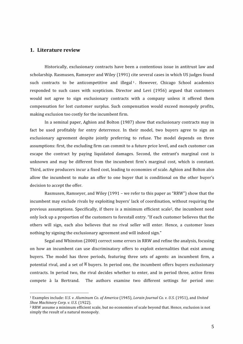
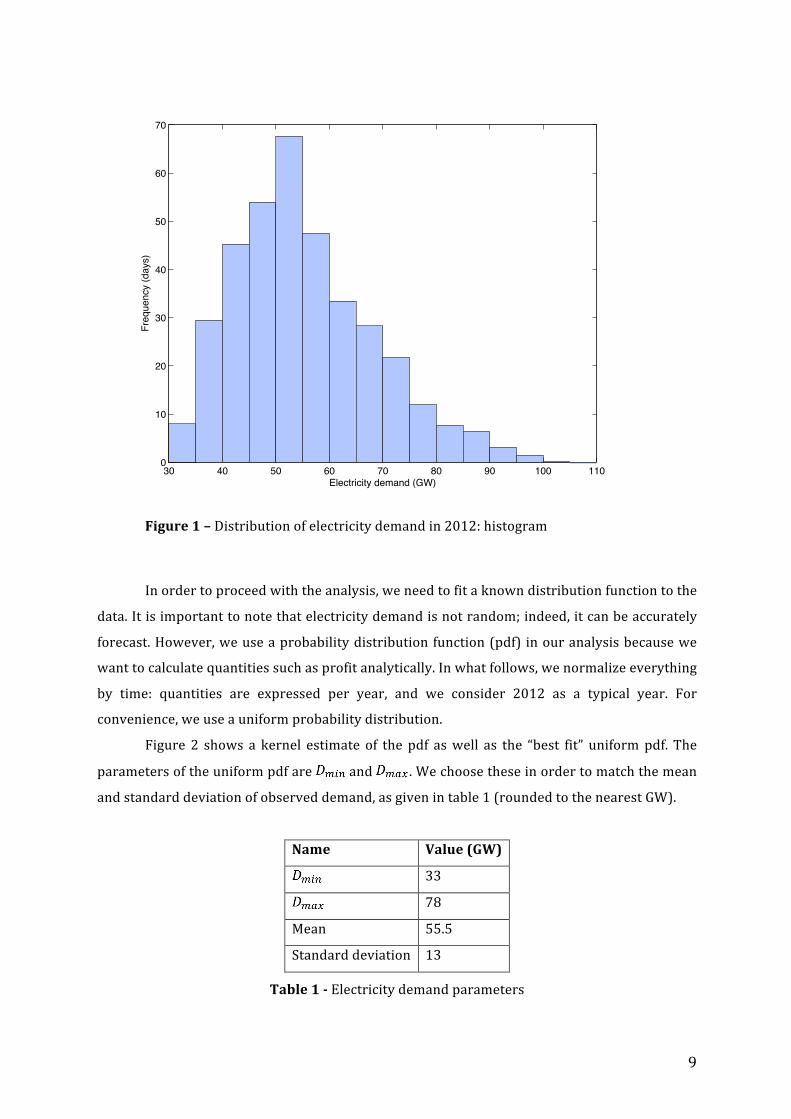
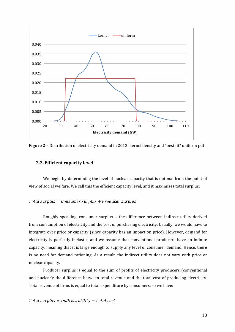
Figure 2 shows a kernel estimate of the pdf as well as the “best fit” uniform pdf. The
parameters of the uniform pdf are and . We choose these in order to match the mean
and standard deviation of observed demand, as given in table 1 (rounded to the nearest GW).
Name Value (GW)
33
78
Mean 55.5
Standard deviation 13
Table 1 -‐ Electricity demand parameters
10
Figure 2 – Distribution of electricity demand in 2012: kernel density and “best fit” uniform pdf
2.2. Efficient capacity level
We begin by determining the level of nuclear capacity that is optimal from the point of
view of social welfare. We call this the efficient capacity level, and it maximizes total surplus:
Roughly speaking, consumer surplus is the difference between indirect utility derived
from consumption of electricity and the cost of purchasing electricity. Usually, we would have to
integrate over price or capacity (since capacity has an impact on price). However, demand for
electricity is perfectly inelastic, and we assume that conventional producers have an infinite
capacity, meaning that it is large enough to supply any level of consumer demand. Hence, there
is no need for demand rationing. As a result, the indirect utility does not vary with price or
nuclear capacity.
Producer surplus is equal to the sum of profits of electricity producers (conventional
and nuclear): the difference between total revenue and the total cost of producing electricity.
Total revenue of firms is equal to total expenditure by consumers, so we have:
11
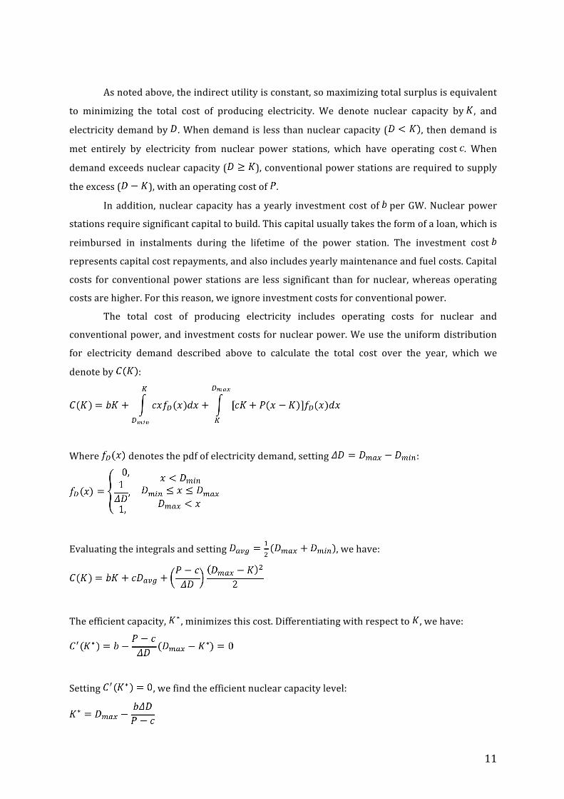
As noted above, the indirect utility is constant, so maximizing total surplus is equivalent
to minimizing the total cost of producing electricity. We denote nuclear capacity by , and
electricity demand by . When demand is less than nuclear capacity ( , then demand is
met entirely by electricity from nuclear power stations, which have operating cost . When
demand exceeds nuclear capacity ( ), conventional power stations are required to supply
the excess ( ), with an operating cost of .
In addition, nuclear capacity has a yearly investment cost of per GW. Nuclear power
stations require significant capital to build. This capital usually takes the form of a loan, which is
reimbursed in instalments during the lifetime of the power station. The investment cost
represents capital cost repayments, and also includes yearly maintenance and fuel costs. Capital
costs for conventional power stations are less significant than for nuclear, whereas operating
costs are higher. For this reason, we ignore investment costs for conventional power.
The total cost of producing electricity includes operating costs for nuclear and
conventional power, and investment costs for nuclear power. We use the uniform distribution
for electricity demand described above to calculate the total cost over the year, which we
denote by :
Where denotes the pdf of electricity demand, setting :
Evaluating the integrals and setting , we have:
The efficient capacity, , minimizes this cost. Differentiating with respect to , we have:
Setting , we find the efficient nuclear capacity level:
12
The efficient capacity depends on the ratio . The denominator is the difference
between conventional and nuclear operating costs; as we will see in the next section, it is also
the difference between the electricity price under monopoly (in the nuclear sector) and the
nuclear operating cost. If , then and : in the absence of
investment costs, the least costly option is for all electricity to be produced from nuclear energy.
On the other hand, if , then and : nuclear capacity is always in
use providing baseload power, while conventional capacity is used to supply , the
variable part of demand.
2.3. Nuclear capacity under monopoly
We now calculate the capacity that maximizes the profit of a nuclear producer with a
monopoly. The conventional sector remains perfectly competitive, but there is a single producer
of nuclear electricity.
The profit of a nuclear monopolist, which we denote , is given by the following
expression, taking into account both operating costs and investment costs:
When , nuclear capacity can cover consumer demand entirely. When demand
exceeds nuclear capacity ( ), nuclear capacity is saturated. Since the conventional sector is
perfectly competitive, the price of electricity produced by conventional means equals its
marginal cost, . Hence, the nuclear monopolist can charge up to for its electricity, and to
maximize profit, it will charge exactly . In theory, consumers would be indifferent between
purchasing nuclear and purchasing conventional electricity if their prices are equal. However,
the network operator prioritizes electricity produced with least marginal cost, so conventional
power stations produce only when nuclear capacity is saturated.
Evaluating the integrals, we find the following expression for monopoly profit:
Differentiating, we have:
13
Setting the derivative to zero, we find the monopoly profit-‐maximizing nuclear capacity:
We notice that the nuclear capacity chosen by a profit-‐maximizing monopolist is equal
to the efficient generating capacity. In other words, the monopoly chooses a nuclear capacity
that minimizes the total cost of producing electricity (including both nuclear and conventional).
The profits earned by the nuclear monopolist and the total cost of producing electricity are
related by:
The sum of monopoly profit and the total cost of producing electricity is , a constant. Hence,
maximizing is equivalent to minimizing . is the total payment from
electricity consumers to electricity producers. Since the nuclear producer charges , the price of
power is whether its source is nuclear or conventional. The payment covers the total cost of
production plus a monopoly rent for the nuclear generator (conventional generators make zero
profit).
We evaluate monopoly profit when , and let . We call this “optimal
profit”. Normalizing by , we have:
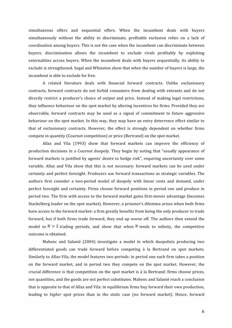
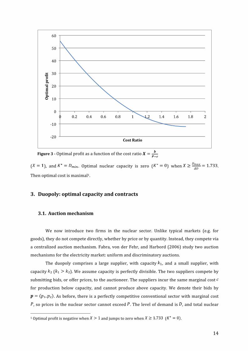
Setting , one can see that maximal profit is a quadratic function of the ratio , which
we call “cost ratio” and denote by . Figure 4 displays this function. As discussed previously,
optimal capacity is a linear decreasing function of . When investment costs are nil ( ,
then , and optimal profit is maximized (optimal cost is minimized). is the
cost of adding a marginal unit of capacity, and is the maximum profit that may be derived
from it (i.e. if the unit operates permanently). Optimal profit is zero when these are equal
14
( ), and . Optimal nuclear capacity is zero ( ) when .
Then optimal cost is maximal1.
3. Duopoly: optimal capacity and contracts
3.1. Auction mechanism
We now introduce two firms in the nuclear sector. Unlike typical markets (e.g. for
goods), they do not compete directly, whether by price or by quantity. Instead, they compete via
a centralized auction mechanism. Fabra, von der Fehr, and Harbord (2006) study two auction
mechanisms for the electricity market: uniform and discriminatory auctions.
The duopoly comprises a large supplier, with capacity , and a small supplier, with
capacity ( ). We assume capacity is perfectly divisible. The two suppliers compete by
submitting bids, or offer prices, to the auctioneer. The suppliers incur the same marginal cost
for production below capacity, and cannot produce above capacity. We denote their bids by
. As before, there is a perfectly competitive conventional sector with marginal cost
, so prices in the nuclear sector cannot exceed . The level of demand is , and total nuclear
1 Optimal profit is negative when and jumps to zero when ( .
Figure 3 -‐ Optimal profit as a function of the cost ratio
15
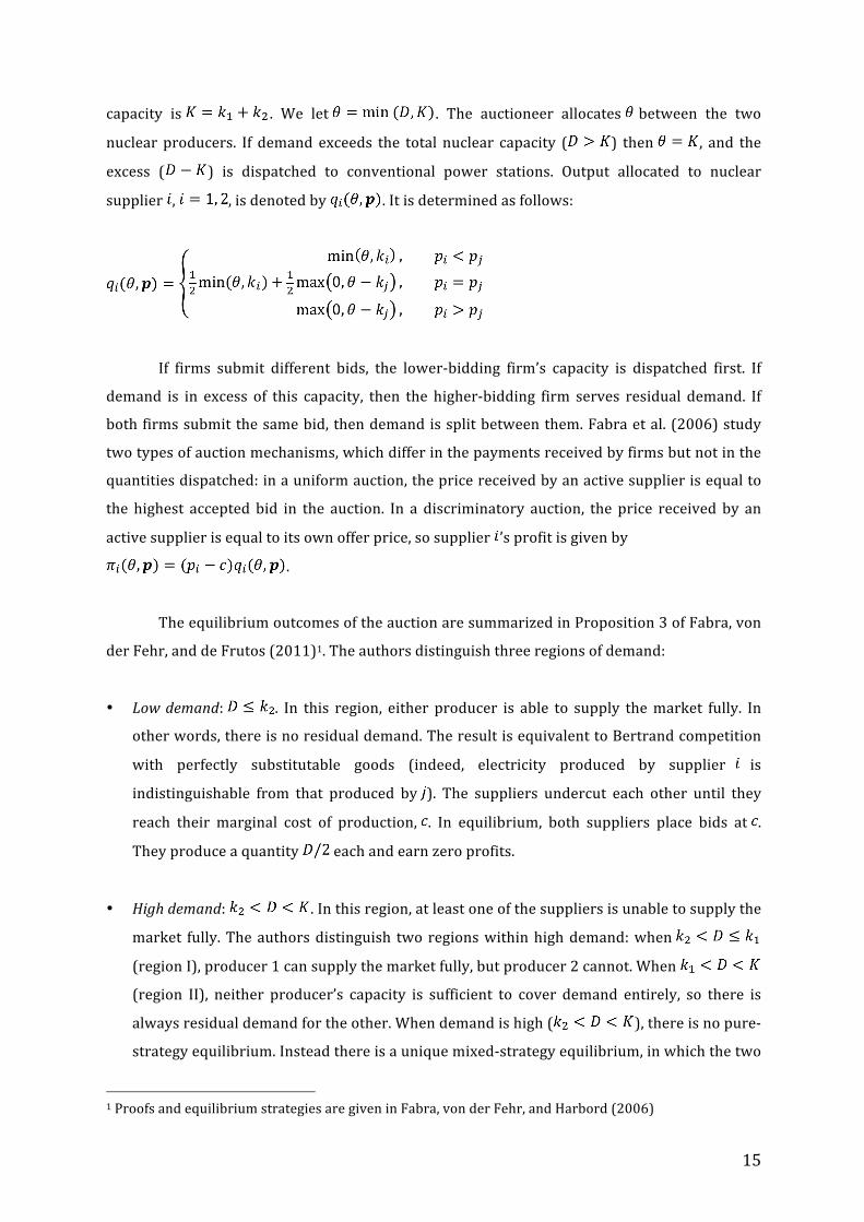
capacity is . We let . The auctioneer allocates between the two
nuclear producers. If demand exceeds the total nuclear capacity ( ) then , and the
excess ( ) is dispatched to conventional power stations. Output allocated to nuclear
supplier , , is denoted by . It is determined as follows:
If firms submit different bids, the lower-‐bidding firm’s capacity is dispatched first. If
demand is in excess of this capacity, then the higher-‐bidding firm serves residual demand. If
both firms submit the same bid, then demand is split between them. Fabra et al. (2006) study
two types of auction mechanisms, which differ in the payments received by firms but not in the
quantities dispatched: in a uniform auction, the price received by an active supplier is equal to
the highest accepted bid in the auction. In a discriminatory auction, the price received by an
active supplier is equal to its own offer price, so supplier ’s profit is given by
.
The equilibrium outcomes of the auction are summarized in Proposition 3 of Fabra, von
der Fehr, and de Frutos (2011)1. The authors distinguish three regions of demand:
• Low demand: . In this region, either producer is able to supply the market fully. In
other words, there is no residual demand. The result is equivalent to Bertrand competition
with perfectly substitutable goods (indeed, electricity produced by supplier is
indistinguishable from that produced by ). The suppliers undercut each other until they
reach their marginal cost of production, . In equilibrium, both suppliers place bids at .
They produce a quantity each and earn zero profits.
• High demand: . In this region, at least one of the suppliers is unable to supply the
market fully. The authors distinguish two regions within high demand: when
(region I), producer 1 can supply the market fully, but producer 2 cannot. When
(region II), neither producer’s capacity is sufficient to cover demand entirely, so there is
always residual demand for the other. When demand is high ( ), there is no pure-‐
strategy equilibrium. Instead there is a unique mixed-‐strategy equilibrium, in which the two
1 Proofs and equilibrium strategies are given in Fabra, von der Fehr, and Harbord (2006)
16
firms mix over a common support that lies above marginal costs and includes . The firms
mix according to different probability distributions: in particular, the large firm has a mass
point at , the upper bound. The small firm bids below with probability 1, so profits of the
large firm are the same as if it offered to sell residual demand at .
• Very high demand: . Nuclear capacity is insufficient to supply the market, so
conventional producers must supply residual demand. In equilibrium, both nuclear firms
place bids at and produce at full capacity.
Intuitively, it is easy to understand why there is no pure-‐strategy equilibrium in the high
demand region. Consider an initial situation where both firms bid . Then either of the suppliers
can increase its profit by placing a bid just below : the increase in output outweighs the
decrease in price. Let firm place a bid just below . Then the other supplier (firm ), serving
residual demand (which may be zero), would benefit by placing a bid just below that of firm .
The firms place subsequently lower bids, until the large firm would profit more from serving
residual demand at than undercutting the small firm. But if the large firm places a bid at , the
small firm will place a bid just below , and so on.
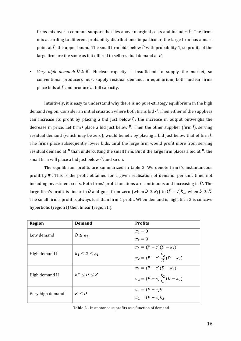
The equilibrium profits are summarized in table 2. We denote firm ’s instantaneous
profit by . This is the profit obtained for a given realisation of demand, per unit time, not
including investment costs. Both firms’ profit functions are continuous and increasing in . The
large firm’s profit is linear in and goes from zero (when ) to , when .
The small firm’s profit is always less than firm 1 profit. When demand is high, firm 2 is concave
hyperbolic (region I) then linear (region II).
Region Demand Profits
Low demand
High demand I
High demand II
Very high demand
Table 2 -‐ Instantaneous profits as a function of demand
17
3.2. Large firm profit and optimal capacity
Having described the auction mechanism and instantaneous profits, we turn our
attention to each firm’s total profit and optimal capacity choice under duopoly. Both firms have
constant marginal costs of investment with a value of .
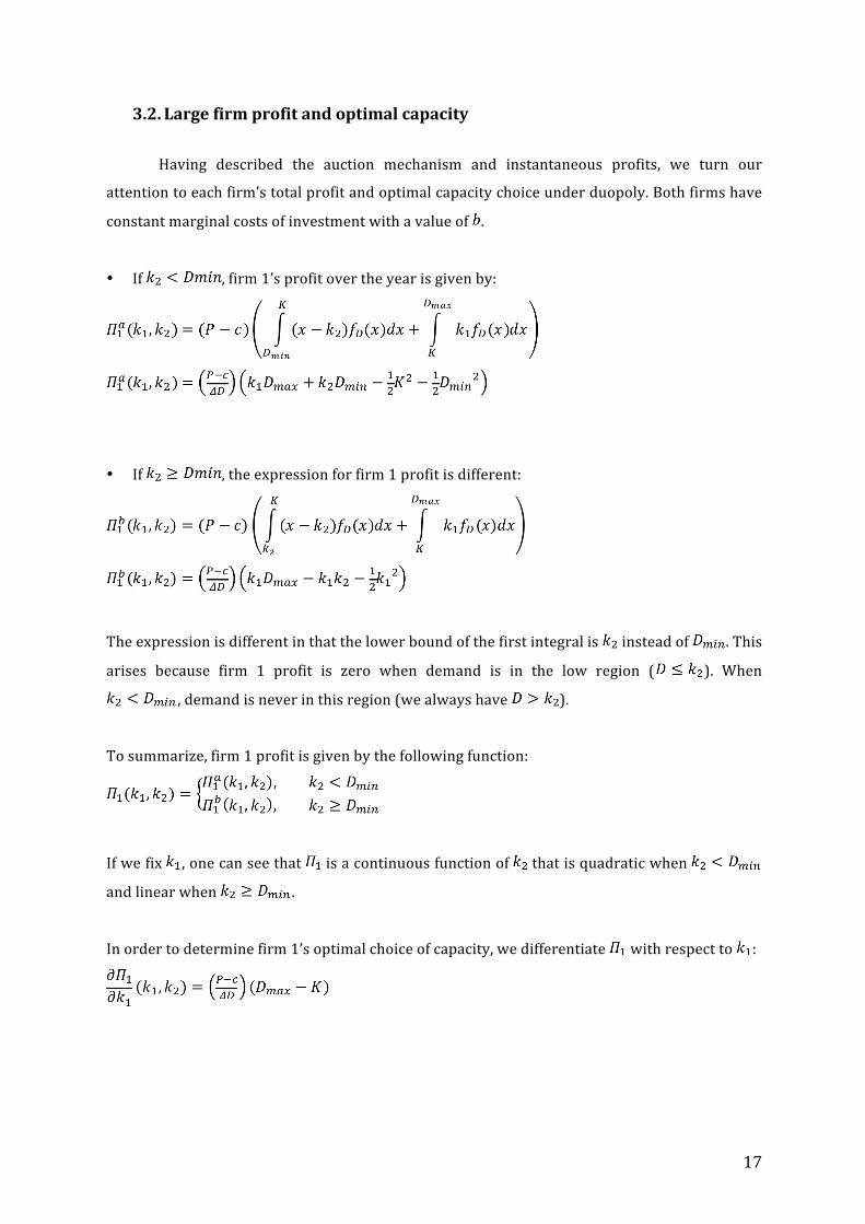
• If , firm 1’s profit over the year is given by:
• If , the expression for firm 1 profit is different:
The expression is different in that the lower bound of the first integral is instead of . This
arises because firm 1 profit is zero when demand is in the low region ( ). When
, demand is never in this region (we always have ).
To summarize, firm 1 profit is given by the following function:
If we fix , one can see that is a continuous function of that is quadratic when
and linear when .
In order to determine firm 1’s optimal choice of capacity, we differentiate with respect to :
18
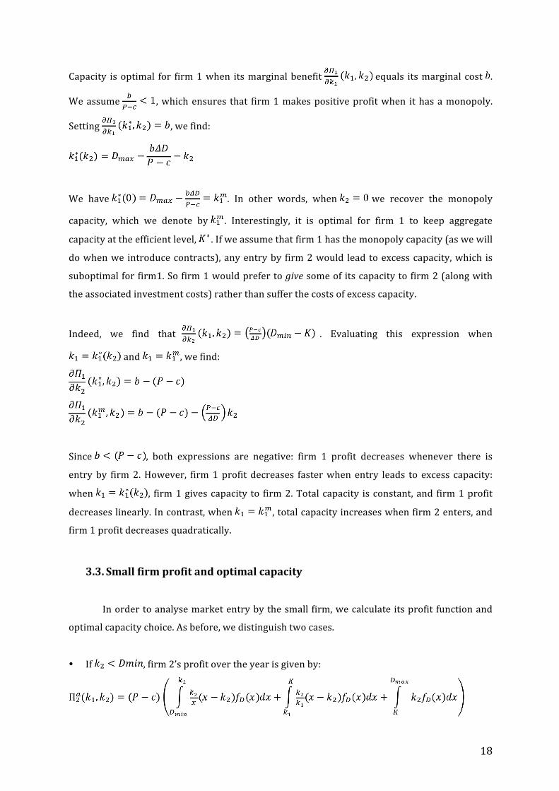
Capacity is optimal for firm 1 when its marginal benefit equals its marginal cost .
We assume , which ensures that firm 1 makes positive profit when it has a monopoly.
Setting , we find:
We have . In other words, when we recover the monopoly
capacity, which we denote by . Interestingly, it is optimal for firm 1 to keep aggregate
capacity at the efficient level, . If we assume that firm 1 has the monopoly capacity (as we will
do when we introduce contracts), any entry by firm 2 would lead to excess capacity, which is
suboptimal for firm1. So firm 1 would prefer to give some of its capacity to firm 2 (along with
the associated investment costs) rather than suffer the costs of excess capacity.
Indeed, we find that . Evaluating this expression when
and , we find:
Since , both expressions are negative: firm 1 profit decreases whenever there is
entry by firm 2. However, firm 1 profit decreases faster when entry leads to excess capacity:
when , firm 1 gives capacity to firm 2. Total capacity is constant, and firm 1 profit
decreases linearly. In contrast, when , total capacity increases when firm 2 enters, and
firm 1 profit decreases quadratically.
3.3. Small firm profit and optimal capacity
In order to analyse market entry by the small firm, we calculate its profit function and
optimal capacity choice. As before, we distinguish two cases.
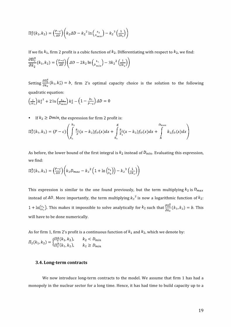
• If , firm 2’s profit over the year is given by:
19
If we fix , firm 2 profit is a cubic function of . Differentiating with respect to , we find:
Setting , firm 2’s optimal capacity choice is the solution to the following
quadratic equation:
• If , the expression for firm 2 profit is:
As before, the lower bound of the first integral is instead of . Evaluating this expression,
we find:
This expression is similar to the one found previously, but the term multiplying is
instead of . More importantly, the term multiplying is now a logarithmic function of :
. This makes it impossible to solve analytically for such that . This
will have to be done numerically.
As for firm 1, firm 2’s profit is a continuous function of and , which we denote by:
3.4. Long-‐term contracts
We now introduce long-‐term contracts to the model. We assume that firm 1 has had a
monopoly in the nuclear sector for a long time. Hence, it has had time to build capacity up to a
20
level that maximises its profit. Hence, we let from now on. The timing of the model is as
follows:
1. Firm 1 has a monopoly and chooses a volume of long-‐term contracts.
2. Firm 2 observes these contracts, and chooses how much capacity to build.
3. The two firms compete on the spot market using the discriminatory auction mechanism
described previously.
The contracts are “long term” in the sense that they are still in effect at the time of entry.
The contracts stipulate that firm 1 supplies a constant level of power to customers
throughout the year at a price . The total capacity supplied to customers under contract
is (we call this the “volume of contracts”). Hence, firm 1 has a capacity available to
compete on the market. As a result, total nuclear capacity on the spot market is reduced to
.
As before, demand is uniformly distributed between and . This is equivalent
to saying that demand is the sum of two components: a constant component and a variable
part ( ) uniformly distributed between and . The constant component represents
baseload power: for example, industrial consumers who use electricity at a constant rate
throughout the year.
Long-‐term supply contracts are signed between such industrial consumers and firm 1.
This removes a volume of capacity from the spot market, so spot market demand is now
distributed between and . We place the following
restrictions on the volume of contracts: must be non-‐negative ( ) and cannot exceed
baseload power ( ). This ensures, respectively, that firm 1 always supplies electricity to
contract customers (never the other way round), and that spot market demand is always
positive.
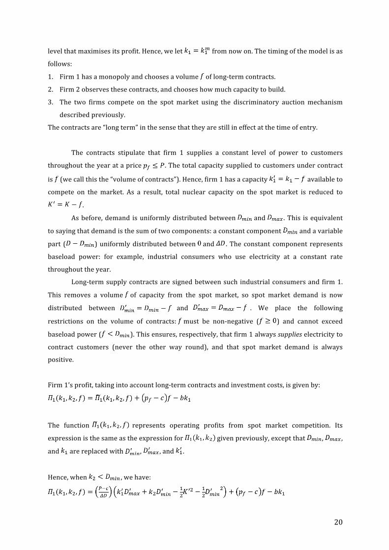
Firm 1’s profit, taking into account long-‐term contracts and investment costs, is given by:
The function represents operating profits from spot market competition. Its
expression is the same as the expression for given previously, except that , ,
and are replaced with , , and .
Hence, when , we have:
21
Developing this expression, we find:
We note that when . One can see that if firm 1 anticipates
that will be small ( ), then firm 1’s motive to sell supply contracts is purely
strategic. Indeed, if we ignore the impact of on firm 2’s choice of capacity (taking as
constant), then firm 1 cannot increase its profit by selling contracts. In fact, its profit will be
reduced if . However, firm 1 may have an incentive to sell contracts if it reduces entry by
firm 2 – this is what we seek to find out.
Similarly to firm 1, firm 2’s profit function, including contracts and investment costs, is:
The expression of is found by replacing , , and with , , and
in the expression of .
We define firm 2’s optimal capacity choice, taking into account contracts, as follows:
Finally, we define and :
22
4. Numerical simulation
4.1. Calibration
We calibrate the model using data for the French electricity market, then simulate using
MATLAB. We have already determined and , the parameters of the electricity demand
distribution. The total nuclear capacity installed in France is 63,130 MW (source: RTE1). We
assume that this capacity was chosen optimally by the monopoly:
GW
We set , using the investment cost as a numéraire, and solve the previous equation to find
. These numbers are summarized in table 3.
Name Value 33 GW 78 GW
63 GW 3
1 (numéraire)
Table 3 – Parameters of the calibrated model
4.2. Monopoly
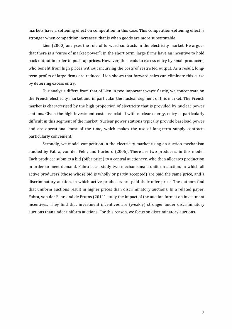
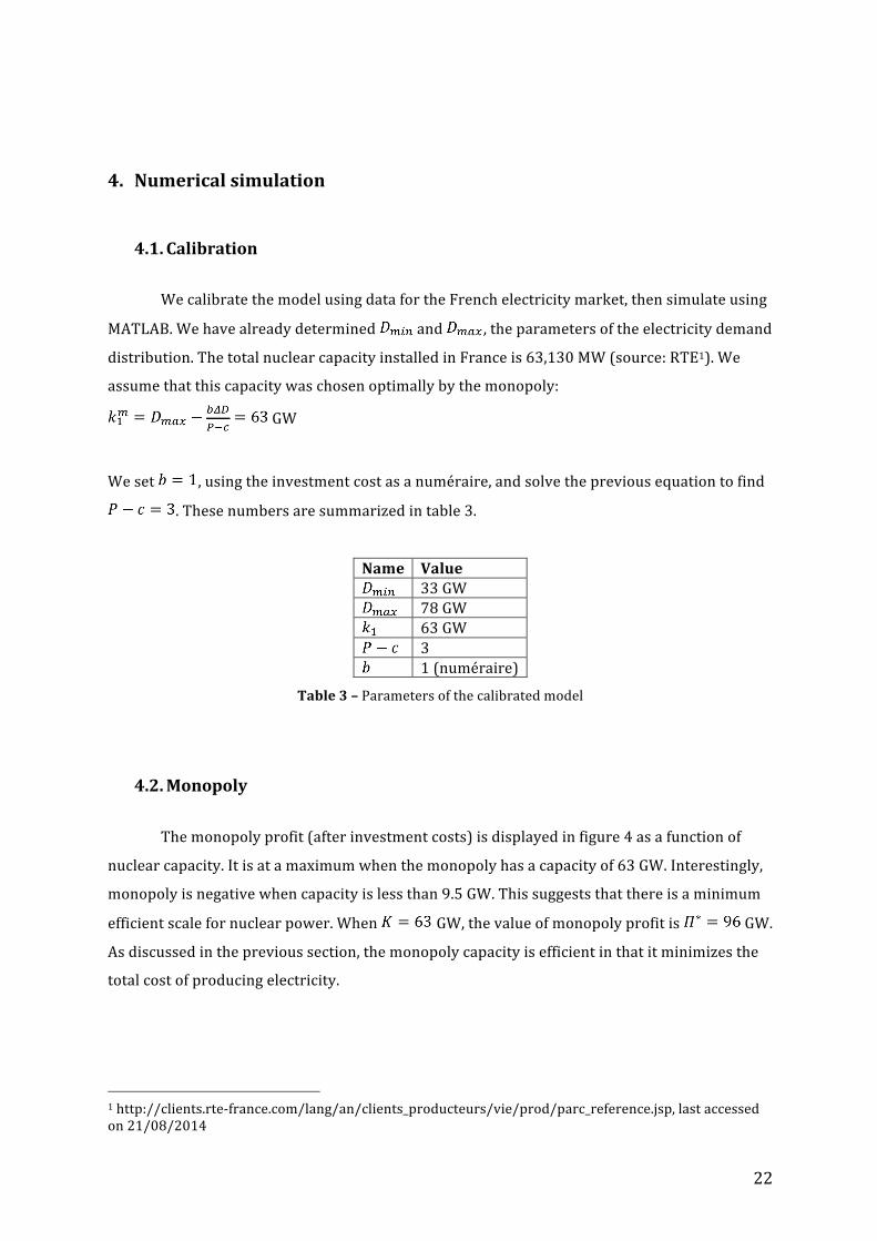
The monopoly profit (after investment costs) is displayed in figure 4 as a function of
nuclear capacity. It is at a maximum when the monopoly has a capacity of 63 GW. Interestingly,
monopoly is negative when capacity is less than 9.5 GW. This suggests that there is a minimum
efficient scale for nuclear power. When GW, the value of monopoly profit is GW.
As discussed in the previous section, the monopoly capacity is efficient in that it minimizes the
total cost of producing electricity.
1 http://clients.rte-‐france.com/lang/an/clients_producteurs/vie/prod/parc_reference.jsp, last accessed on 21/08/2014
23
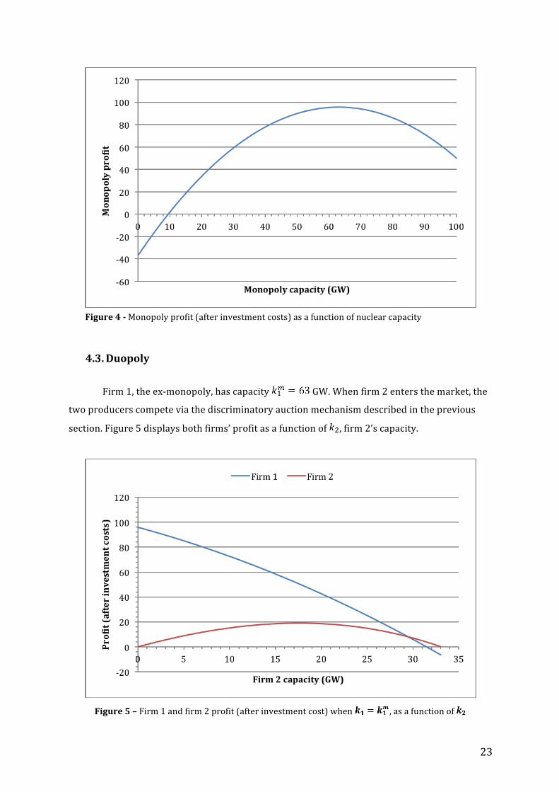
4.3. Duopoly
Firm 1, the ex-‐monopoly, has capacity GW. When firm 2 enters the market, the
two producers compete via the discriminatory auction mechanism described in the previous
section. Figure 5 displays both firms’ profit as a function of , firm 2’s capacity.
Figure 5 – Firm 1 and firm 2 profit (after investment cost) when , as a function of
Figure 4 -‐ Monopoly profit (after investment costs) as a function of nuclear capacity
24
Firm 1 profit is strictly decreasing in , and becomes negative when GW. In
the absence of contracts, firm 2 profit is maximum when GW, so we have GW.
At this point, firm 1 makes a profit of 51, about half of monopoly profit. We notice that firm 2
makes non-‐negative profit as long as , which implies that there is no minimum
efficient scale for firm 2. This is because we have not given firm 2 any fixed costs – investment
costs are proportional to capacity. However, if firm 2 had fixed costs of say 10, then capacity
below 5 GW would not be profitable.
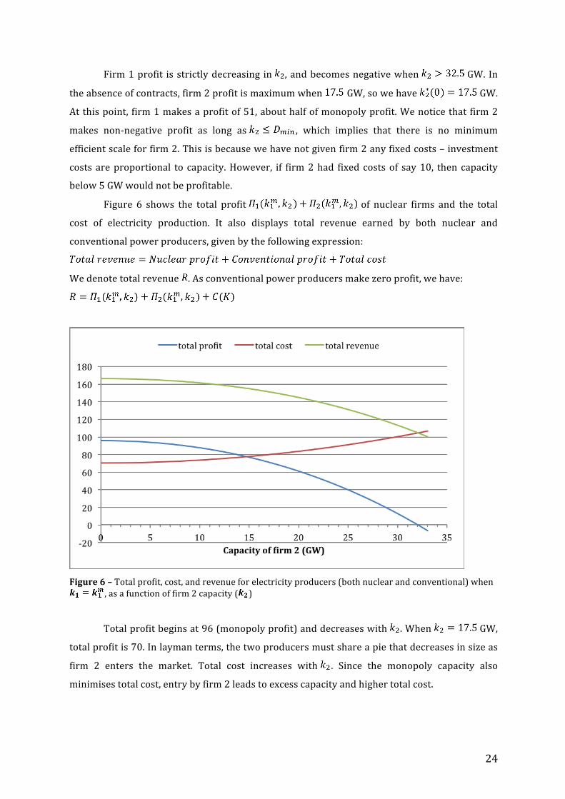
Figure 6 shows the total profit of nuclear firms and the total
cost of electricity production. It also displays total revenue earned by both nuclear and
conventional power producers, given by the following expression:
We denote total revenue . As conventional power producers make zero profit, we have:
Figure 6 – Total profit, cost, and revenue for electricity producers (both nuclear and conventional) when
, as a function of firm 2 capacity ( )
Total profit begins at 96 (monopoly profit) and decreases with . When GW,
total profit is 70. In layman terms, the two producers must share a pie that decreases in size as
firm 2 enters the market. Total cost increases with . Since the monopoly capacity also
minimises total cost, entry by firm 2 leads to excess capacity and higher total cost.
25
Total revenue decreases with , which implies that the decrease in total profit is not
only associated with increased cost of electricity production. There is also a price effect. We
define a price index by the following expression: .
This index of the wholesale price of electricity is proportional to total revenue.
when , and when GW. Hence, market entry by firm 2
leads to higher total cost of electricity, and lower total profit and revenue. The price of
electricity decreases by approximately 10%.
4.4. Long-‐term contracts
We now allow firm 1 to hold a volume of long-‐term supply contracts, according to
which firm 1 supplies electricity at a price . At the time of signing the contracts, firm 1
has a monopoly and the price of electricity is , so customers are indifferent between
purchasing electricity on the market and a contract where . We set and calculate
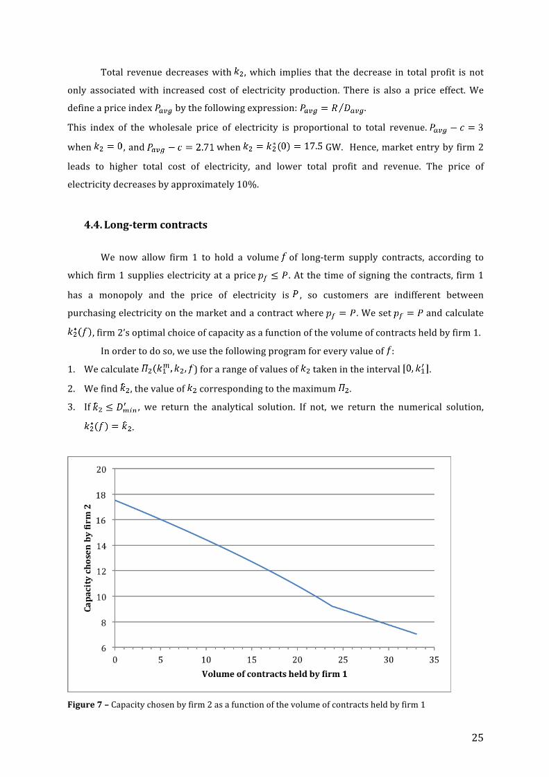
, firm 2’s optimal choice of capacity as a function of the volume of contracts held by firm 1.
In order to do so, we use the following program for every value of :
1. We calculate ) for a range of values of taken in the interval .
2. We find , the value of corresponding to the maximum .
3. If , we return the analytical solution. If not, we return the numerical solution,
.
Figure 7 – Capacity chosen by firm 2 as a function of the volume of contracts held by firm 1
26
Figure 7 displays for . The capacity chosen by firm 2 is strictly
decreasing in . There is a change in slope when GW. Beyond this point, .
As discussed in the previous section, the profit functions of the firms change when .
As a result, the slope of changes.
We note that the reduction in firm 2’s capacity is approximately proportional to ,
the volume of contracts expressed as a proportion of firm 1 capacity. Indeed, when
, firm 2’s capacity is reduced by 58%.
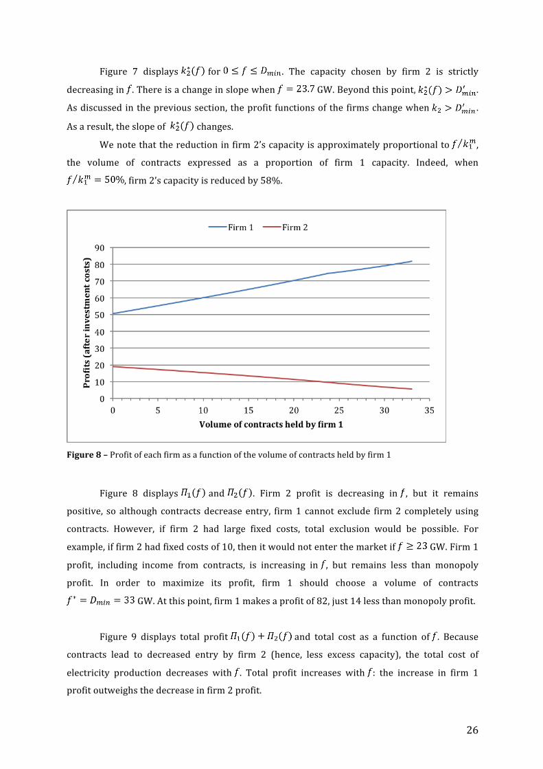
Figure 8 – Profit of each firm as a function of the volume of contracts held by firm 1
Figure 8 displays and . Firm 2 profit is decreasing in , but it remains
positive, so although contracts decrease entry, firm 1 cannot exclude firm 2 completely using
contracts. However, if firm 2 had large fixed costs, total exclusion would be possible. For
example, if firm 2 had fixed costs of 10, then it would not enter the market if GW. Firm 1
profit, including income from contracts, is increasing in , but remains less than monopoly
profit. In order to maximize its profit, firm 1 should choose a volume of contracts
GW. At this point, firm 1 makes a profit of 82, just 14 less than monopoly profit.
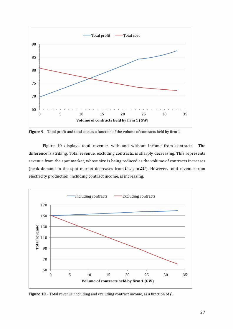
Figure 9 displays total profit and total cost as a function of . Because
contracts lead to decreased entry by firm 2 (hence, less excess capacity), the total cost of
electricity production decreases with . Total profit increases with : the increase in firm 1
profit outweighs the decrease in firm 2 profit.
27
Figure 10 displays total revenue, with and without income from contracts. The
difference is striking. Total revenue, excluding contracts, is sharply decreasing. This represents
revenue from the spot market, whose size is being reduced as the volume of contracts increases
(peak demand in the spot market decreases from to ). However, total revenue from
electricity production, including contract income, is increasing.
Figure 10 – Total revenue, including and excluding contract income, as a function of .
Figure 9 – Total profit and total cost as a function of the volume of contracts held by firm 1
28
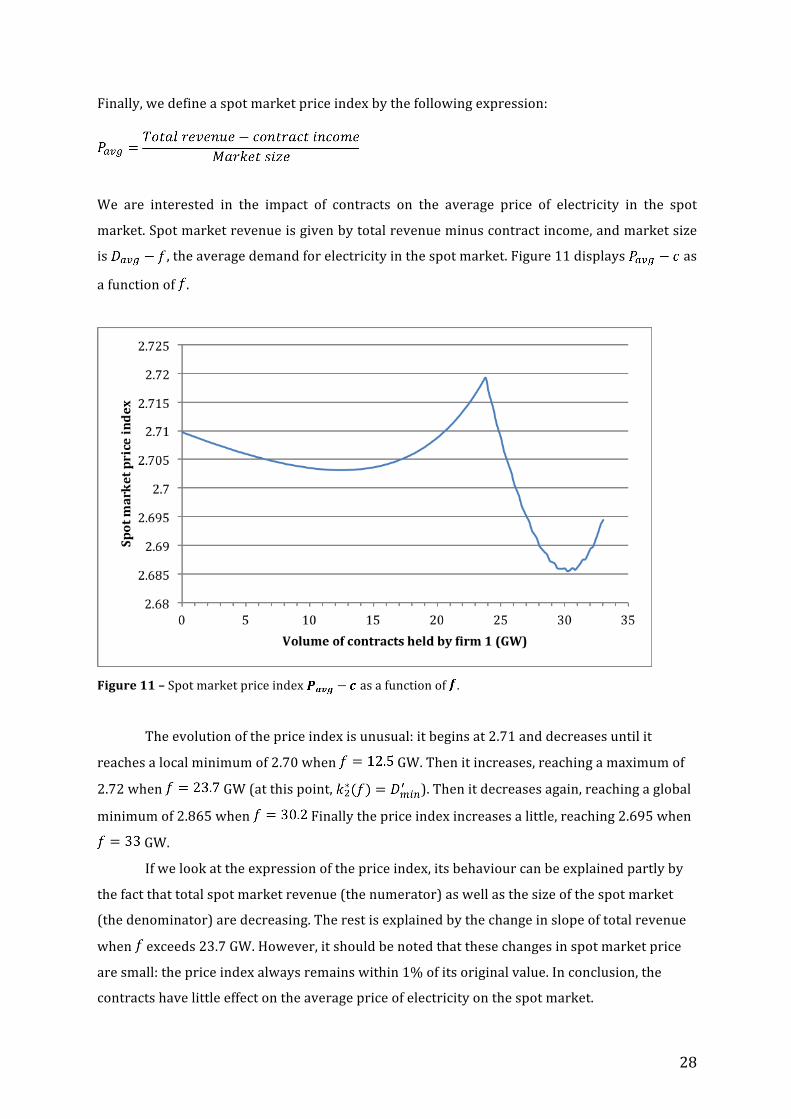
Finally, we define a spot market price index by the following expression:
We are interested in the impact of contracts on the average price of electricity in the spot
market. Spot market revenue is given by total revenue minus contract income, and market size
is , the average demand for electricity in the spot market. Figure 11 displays as
a function of .
Figure 11 – Spot market price index as a function of .
The evolution of the price index is unusual: it begins at 2.71 and decreases until it
reaches a local minimum of 2.70 when GW. Then it increases, reaching a maximum of
2.72 when GW (at this point, ). Then it decreases again, reaching a global
minimum of 2.865 when Finally the price index increases a little, reaching 2.695 when
GW.
If we look at the expression of the price index, its behaviour can be explained partly by
the fact that total spot market revenue (the numerator) as well as the size of the spot market
(the denominator) are decreasing. The rest is explained by the change in slope of total revenue
when exceeds 23.7 GW. However, it should be noted that these changes in spot market price
are small: the price index always remains within 1% of its original value. In conclusion, the
contracts have little effect on the average price of electricity on the spot market.
29
Conclusion
In our model, the French electricity market is made up of two sectors: a perfectly
competitive conventional sector and a nuclear sector. Electricity demand is uniformly
distributed. We focus our analysis on market entry in the nuclear sector. We begin by
determining the nuclear capacity that a monopoly would choose in order to maximize its profit.
This capacity also minimizes the total cost of producing electricity (from both conventional and
nuclear sources) to meet consumer demand.
We then consider what happens when there are two nuclear producers: a large firm, the
incumbent, and a small firm, the entrant. The two firms compete via a discriminatory auction
mechanism described in Fabra et al. (2006). When demand is less than the small firm capacity,
both firms sell capacity at marginal cost and make zero profit. When demand exceeds total
nuclear capacity, each firm supplies its whole capacity at the marginal cost of conventional
producers. When demand is between these two regions, there is a mixed strategy equilibrium.
We find expressions for each firm’s yearly profit by integrating over the distribution of
demand. We then calibrate the model to the French market, assuming that the nuclear capacity
installed on the market (63 GW) is the monopoly profit-‐maximizing capacity. In the absence of
contracts, the small firm maximizes its profit by installing a capacity of 17.5 GW. Since the
monopoly capacity is efficient, market entry leads to excess capacity: the total cost of producing
electricity increases. Total profit and revenue decrease, and the average price of electricity
drops by 10%.
We then allow the incumbent to sign long-‐term contracts with industrial consumers
before the small firm enters the market. According to these contracts, the incumbent supplies a
constant capacity at a price . We assume that – the contract price is equal to the price
of electricity at the time the contracts are signed (when the incumbent has a monopoly). As the
volume of contracts increases, market entry by the small firm is reduced. Its profit decreases,
while the incumbent’s profit increases. However, the incumbent cannot recover monopoly
profit entirely. Furthermore, contracts reduce market entry, but they cannot exclude rivals
entirely unless the entrant has large fixed costs.
From a welfare point of view, the effect of long-‐term contracts is ambiguous. On the one
hand, market entry leads to excess capacity, so by limiting entry the contracts help to minimize
the cost of electricity production. However, market entry reduces the price of electricity, which
may be viewed as beneficial for consumers. Interestingly, long-‐term contracts do not have a
significant effect on the price of electricity on the spot market: it remains near the level it would
30
have had with unrestricted market entry. However, customers who have signed long-‐term
contracts continue to pay the monopoly price for electricity. As a result, they have an incentive
to escape the contract in order to purchase electricity on the spot market instead.
An important extension of this work would be to consider customers’ incentives to sign
contracts. We have assumed that at the time of signing, customers do not anticipate that there
will be market entry, or they do not internalize the consequences that the contracts will have on
a rival producer’s decision to enter the market. If they were to anticipate this, how could the
incumbent producer incentivise them to sign the contract? A possible answer would be to look
at the contract price . Perhaps the incumbent could offer customers a discount at the time of
signing (setting ), but in that case would the incumbent still benefit from having the
contracts? Similarly, one could look at how the contracts should be structured in order to
dissuade customers from ending them after they observe market entry and the resulting lower
prices. A first step would be to examine the penalty that firms would be required to pay in the
event of a premature termination of the contract.
31
References
Aghion, Philippe, and Patrick Bolton. "Contracts as a Barrier to Entry." American Economic
Review (1987): 388-‐401.
Allaz, Blaise, and Jean-‐Luc Vila. "Cournot competition, forward markets and efficiency." Journal
of Economic Theory 59, no. 1 (1993): 1-‐16.
Bessot, Nicolas, Maciej Ciszewski, and Augustijn Van Haasteren. "The EDF long term contracts
case: addressing foreclosure for the long term benefit of industrial customers." Competition
Policy Newsletter 2 (2010): 10-‐13.
Director, Aaron, and Edward H. Levi. "Law and the future: Trade regulation." Northwestern
University Law Review 51 (1956): 281.
Lien, J. “Forward Contracts and the Curse of Market Power”, University of Maryland Working
Paper (2000)
Mahenc, Philippe, and François Salanié. "Softening competition through forward trading."
Journal of Economic Theory 116, no. 2 (2004): 282-‐293.
Fabra, Natalia, Nils-‐Henrik von der Fehr, and David Harbord. "Designing electricity auctions."
RAND Journal of Economics 37, no. 1 (2006): 23-‐46.
Fabra, Natalia, Nils-‐Henrik von der Fehr, and María-‐Ángeles de Frutos. "Market Design and
Investment Incentives." Economic Journal 121, no. 557 (2011): 1340-‐1360.
Rasmusen, Eric B., J. Mark Ramseyer, and John S. Wiley Jr. "Naked Exclusion." American
Economic Review (1991): 1137-‐1145.
Segal, Ilya R., and Michael D. Whinston. "Naked Exclusion: Comment." American Economic
Review (2000): 296-‐309.
32
Appendix – selected MATLAB code Function function [k2opt,profit2] = maxprofit2(f) %MAXPROFIT2 Returns the level of capacity that maximizes firm 2's profit, %when firm 1 has capacity k1m and holds a volume of contract f Dmin = 33 - f; Dmax = 78 - f; DeltaD = Dmax - Dmin; % k1 is the monopoly capacity, given by k1 = Dmax - b*DeltaD/(P-c) k1 = 63 - f; % investment cost (numeraire price) b = 1; % NetPrice = P - c NetPrice = b*DeltaD/(Dmax - k1); % maximum capacity of firm 2 - we do not want k2 to exceed k1 k2max = Dmax; % step size (number of data points = k2max/step + 1) step = 0.01; % capacity of firm 2 k2vector = 0:step:k2max; % initializing Profit2 = zeros(size(k2vector)); NetProfit2 = zeros(size(k2vector)); for i = 1:length(k2vector) k2 = k2vector(i); K = k1 + k2; % parameters for firm 2 profit A = 3/(2*k1); B1 = 2*log(k1/Dmin); % B1 and B2 are minus infty if f = 63 B2 = 1 + log(k1/k2); C = -(1-b/NetPrice)*DeltaD; if k2 <= Dmin % profit of firm 2, before and after fixed costs Profit2(i) = NetPrice/DeltaD*(DeltaD*k2 - B1/2*k2^2 - A/3*k2^3); NetProfit2(i) = Profit2(i) - b*k2; % net of fixed cost else % profit of firm 2, before and after fixed costs Profit2(i) = NetPrice/DeltaD*(Dmax*k2 - B2*k2^2 - A/3*k2^3); NetProfit2(i) = Profit2(i) - b*k2; % net of fixed cost end end profit2 = max(NetProfit2); k2opt = k2vector(NetProfit2 == profit2);
33
if k2opt <= Dmin % overwrite k2opt and profit2 with analytical solution (more precise) k2opt = (-B1 + sqrt(B1^2-4*A*C))/(2*A); profit2 = NetPrice/DeltaD*(DeltaD*k2opt - B1/2*k2opt^2 - A/3*k2opt^3)... - b*k2opt; end end
Main script (calls the previous function) % calculates the optimal capacity chosen by firm 2 as a function of the % volume of contracts held by firm 1, where firm 1 has the monopoly % capacity. Also calculates resulting profit of both firms. Dmin = 33; Dmax = 78; DeltaD = Dmax - Dmin; Davg = (Dmax + Dmin)/2; % k1 is the monopoly capacity, given by k1 = Dmax - b*DeltaD/(P-c) k1 = 63; % Investment cost (numeraire price) b = 1; % NetPrice = P - c NetPrice = b*DeltaD/(Dmax - k1); % Discount = (pf - c)/(P - c) Discount = 1; ContractPrice = Discount*NetPrice; % maximum volume of contracts (must be < 63) fmax = 33; % step size (number of data points = fmax/step + 1) step = 0.2; % volume of contracts fvector = 0:step:fmax; % initializing k2vector = zeros(size(fvector)); Profit1 = zeros(size(fvector)); NetProfit1 = zeros(size(fvector)); Profit2 = zeros(size(fvector)); NetProfit2 = zeros(size(fvector)); TotalCost = zeros(size(fvector)); for i = 1:length(fvector) % volume of contracts f = fvector(i); % updated quantities Dmaxp = Dmax - f; Dminp = Dmin - f; k1p = k1 - f;
34
% firm 2 capacity and profits [k2,NetProfit2(i)] = maxprofit2(f); k2vector(i) = k2; Profit2(i) = NetProfit2(i) + b*k2; % total capacity K = k1 + k2; Kp = K - f; % profit of firm 1, before and after fixed costs if k2 < Dminp Profit1(i) = NetPrice/DeltaD*(k1p*Dmaxp + k2*Dminp... - 1/2*Kp^2 -1/2*Dminp^2) + ContractPrice*f; else Profit1(i) = NetPrice/DeltaD*(k1p*(Dmaxp-k2) - 1/2*k1p^2)... + ContractPrice*f; end NetProfit1(i) = Profit1(i) - b*k1; % net of fixed cost % total production cost minus c*Davg TotalCost(i) = b*K + NetPrice/DeltaD*0.5*(Dmax-K)^2; end % total profit = firm 1 + firm 2 + coal (zero profit) TotalProfit = NetProfit1 + NetProfit2; % after investment costs % PriceAvg = Pavg - c (retail price index net of operating cost) PriceAvg = (TotalProfit + TotalCost - ContractPrice*fvector)./(Davg - fvector);