Hashing

Ing. Juan Ignacio Zamora M. MS.c Facultad de Ingenierías Licenciatura en Ingeniería Informática con Énfasis en Desarrollo de Software Universidad Latinoamericana de Ciencia y Tecnología

Que es Hashing?

�  Hashing es un concepto programático que refiera al direccionamiento que se realiza a partir del valor (llave or key) hacia un campo en una estructura de datos de composición estática o dinámica.

Hashing – Direct Address

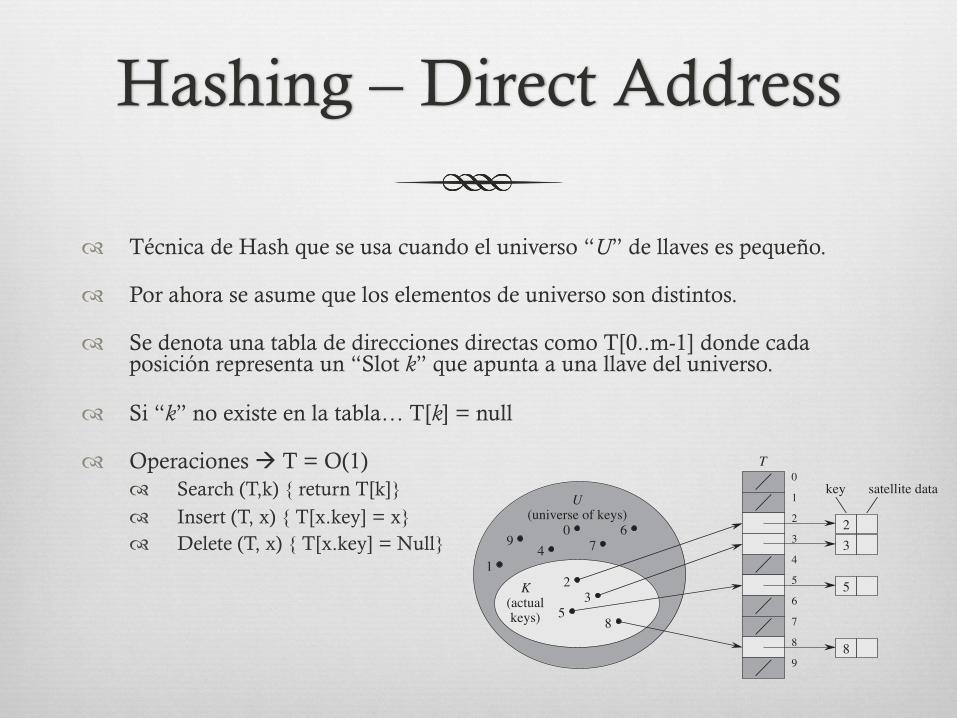
�  Técnica de Hash que se usa cuando el universo “U” de llaves es pequeño.

�  Por ahora se asume que los elementos de universo son distintos.

�  Se denota una tabla de direcciones directas como T[0..m-1] donde cada posición representa un “Slot k” que apunta a una llave del universo.

�  Si “k” no existe en la tabla… T[k] = null

�  Operaciones à T = O(1) �  Search (T,k) { return T[k]} �  Insert (T, x) { T[x.key] = x} �  Delete (T, x) { T[x.key] = Null}

254 Chapter 11 Hash Tables

11.1 Direct-address tables

Direct addressing is a simple technique that works well when the universe U ofkeys is reasonably small. Suppose that an application needs a dynamic set in whicheach element has a key drawn from the universe U D f0; 1; : : : ; m ! 1g, where mis not too large. We shall assume that no two elements have the same key.

To represent the dynamic set, we use an array, or direct-address table, denotedby T Œ0 : : m ! 1!, in which each position, or slot, corresponds to a key in the uni-verse U . Figure 11.1 illustrates the approach; slot k points to an element in the setwith key k. If the set contains no element with key k, then T Œk! D NIL.

The dictionary operations are trivial to implement:DIRECT-ADDRESS-SEARCH.T; k/

1 return T Œk!

DIRECT-ADDRESS-INSERT.T; x/

1 T Œx:key! D x

DIRECT-ADDRESS-DELETE.T; x/

1 T Œx:key! D NIL

Each of these operations takes only O.1/ time.

T

U(universe of keys)

K(actualkeys)

23

5 8

19 4

07

6 23

5

8

key satellite data2

01

3456789

Figure 11.1 How to implement a dynamic set by a direct-address table T . Each key in the universeU D f0; 1; : : : ; 9g corresponds to an index in the table. The set K D f2; 3; 5; 8g of actual keysdetermines the slots in the table that contain pointers to elements. The other slots, heavily shaded,contain NIL.

Hashing - Hash Table

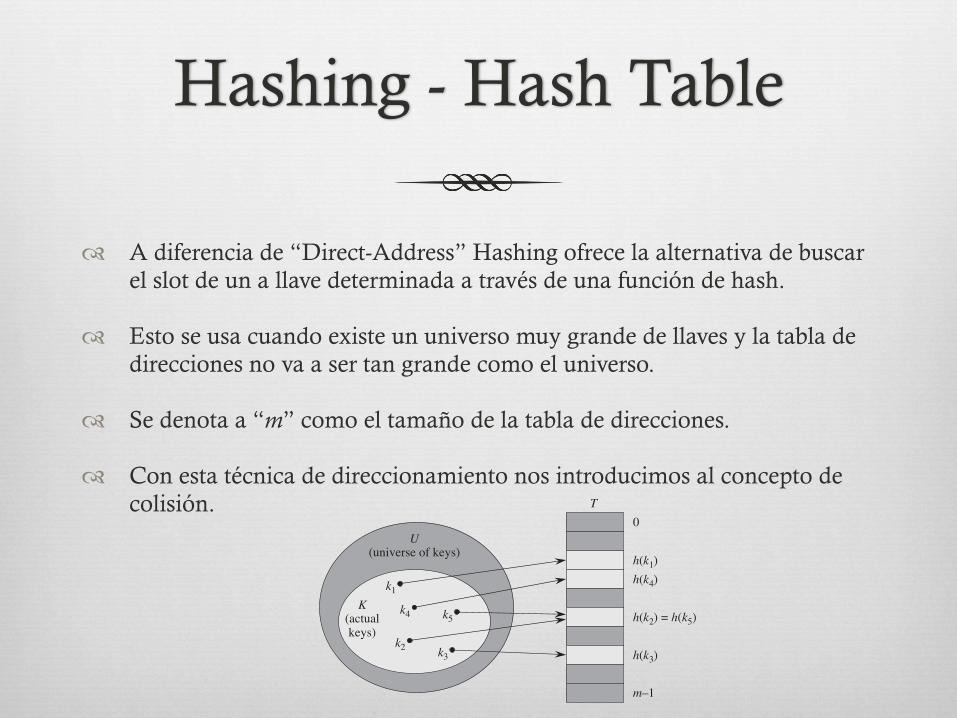
�  A diferencia de “Direct-Address” Hashing ofrece la alternativa de buscar el slot de un a llave determinada a través de una función de hash.

�  Esto se usa cuando existe un universo muy grande de llaves y la tabla de direcciones no va a ser tan grande como el universo.

�  Se denota a “m” como el tamaño de la tabla de direcciones.

�  Con esta técnica de direccionamiento nos introducimos al concepto de colisión.


11.2 Hash tables

The downside of direct addressing is obvious: if the universe U is large, storinga table T of size jU j may be impractical, or even impossible, given the memoryavailable on a typical computer. Furthermore, the set K of keys actually storedmay be so small relative to U that most of the space allocated for T would bewasted.

When the set K of keys stored in a dictionary is much smaller than the uni-verse U of all possible keys, a hash table requires much less storage than a direct-address table. Specifically, we can reduce the storage requirement to ‚.jKj/ whilewe maintain the benefit that searching for an element in the hash table still requiresonly O.1/ time. The catch is that this bound is for the average-case time, whereasfor direct addressing it holds for the worst-case time.

With direct addressing, an element with key k is stored in slot k. With hashing,this element is stored in slot h.k/; that is, we use a hash function h to compute theslot from the key k. Here, h maps the universe U of keys into the slots of a hashtable T Œ0 : : m ! 1!:h W U ! f0; 1; : : : ; m ! 1g ;

where the size m of the hash table is typically much less than jU j. We say that anelement with key k hashes to slot h.k/; we also say that h.k/ is the hash value ofkey k. Figure 11.2 illustrates the basic idea. The hash function reduces the rangeof array indices and hence the size of the array. Instead of a size of jU j, the arraycan have size m.

T

U(universe of keys)

K(actualkeys)

0

m–1

k1

k2 k3

k4 k5

h(k1)h(k4)

h(k3)

h(k2) = h(k5)

Figure 11.2 Using a hash function h to map keys to hash-table slots. Because keys k2 and k5 mapto the same slot, they collide.

Colisiones

�  Se da una colisión cuando 2 o mas llaves apuntan al mismo slot.

�  Lo ideal es evitar las colisiones, sin embargo no en todas* las implementaciones se logra…

�  Se intenta entonces crear una función de hash que sea lo suficiente mente aleatoria para siempre crear una dirección única para cada valor y evitar las colisiones…

Aleatoriedad

�  Realmente existe?

�  Cuantas teclas hay en su teclado? �  26 letras �  14 teclas de puntuación �  Mas para numeración y comandos adicionales

�  Realmente una moneda cae 50% de la veces de un lado especifico.

�  El rebote de una bola es aleatorio?

�  Es el tiempo una medida aleatoria?

�  Cual es la posibilidad de sacar “5” en un juego de dados? *

Resolucion de Colisiones Por Encadenamiento

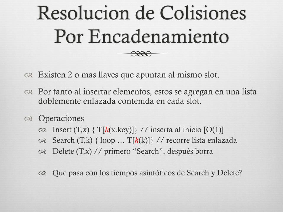
�  Existen 2 o mas llaves que apuntan al mismo slot.

�  Por tanto al insertar elementos, estos se agregan en una lista doblemente enlazada contenida en cada slot.

�  Operaciones �  Insert (T,x) { T[h(x.key)]} // inserta al inicio [O(1)] �  Search (T,k) { loop … T[h(k)]} // recorre lista enlazada �  Delete (T,x) // primero “Search”, después borra

�  Que pasa con los tiempos asintóticos de Search y Delete?

Search & Delete

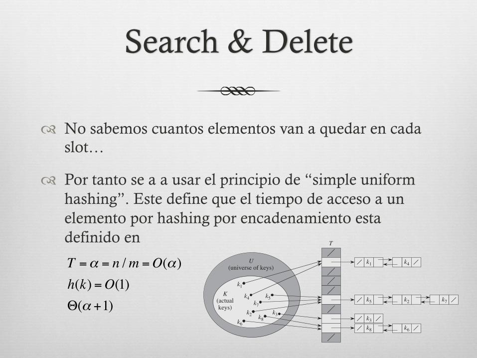
�  No sabemos cuantos elementos van a quedar en cada slot…

�  Por tanto se a a usar el principio de “simple uniform hashing”. Este define que el tiempo de acceso a un elemento por hashing por encadenamiento esta definido en

11.2 Hash tables 257

T

U(universe of keys)

K(actualkeys)

k1

k2 k3

k4 k5

k6

k7

k8

k1

k2

k3

k4

k5

k6

k7

k8

Figure 11.3 Collision resolution by chaining. Each hash-table slot T Œj ! contains a linked list ofall the keys whose hash value is j . For example, h.k1/ D h.k4/ and h.k5/ D h.k7/ D h.k2/.The linked list can be either singly or doubly linked; we show it as doubly linked because deletion isfaster that way.

There is one hitch: two keys may hash to the same slot. We call this situationa collision. Fortunately, we have effective techniques for resolving the conflictcreated by collisions.

Of course, the ideal solution would be to avoid collisions altogether. We mighttry to achieve this goal by choosing a suitable hash function h. One idea is tomake h appear to be “random,” thus avoiding collisions or at least minimizingtheir number. The very term “to hash,” evoking images of random mixing andchopping, captures the spirit of this approach. (Of course, a hash function h must bedeterministic in that a given input k should always produce the same output h.k/.)Because jU j > m, however, there must be at least two keys that have the same hashvalue; avoiding collisions altogether is therefore impossible. Thus, while a well-designed, “random”-looking hash function can minimize the number of collisions,we still need a method for resolving the collisions that do occur.

The remainder of this section presents the simplest collision resolution tech-nique, called chaining. Section 11.4 introduces an alternative method for resolvingcollisions, called open addressing.

Collision resolution by chainingIn chaining, we place all the elements that hash to the same slot into the samelinked list, as Figure 11.3 shows. Slot j contains a pointer to the head of the list ofall stored elements that hash to j ; if there are no such elements, slot j contains NIL.

T =α = n /m =O(α)h(k) =O(1)Θ(α +1)

Donde esta la Magia – Función de Hash [h(k)]

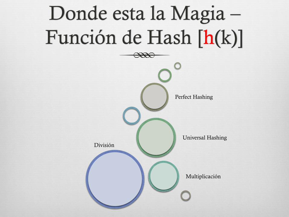
División

Multiplicación

Universal Hashing

Perfect Hashing

Método : División

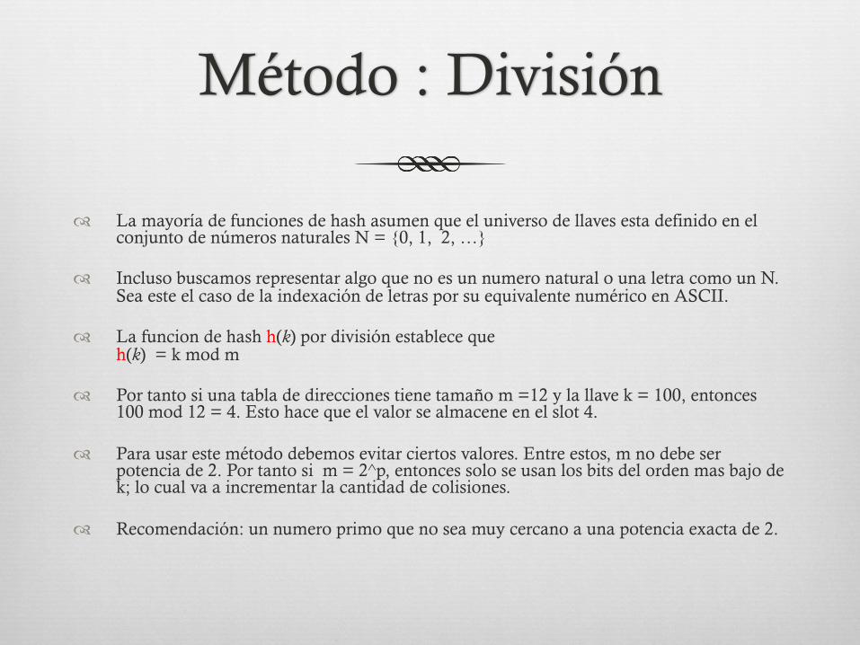
�  La mayoría de funciones de hash asumen que el universo de llaves esta definido en el conjunto de números naturales N = {0, 1, 2, …}

�  Incluso buscamos representar algo que no es un numero natural o una letra como un N. Sea este el caso de la indexación de letras por su equivalente numérico en ASCII.

�  La funcion de hash h(k) por división establece que h(k) = k mod m

�  Por tanto si una tabla de direcciones tiene tamaño m =12 y la llave k = 100, entonces 100 mod 12 = 4. Esto hace que el valor se almacene en el slot 4.

�  Para usar este método debemos evitar ciertos valores. Entre estos, m no debe ser potencia de 2. Por tanto si m = 2^p, entonces solo se usan los bits del orden mas bajo de k; lo cual va a incrementar la cantidad de colisiones.

�  Recomendación: un numero primo que no sea muy cercano a una potencia exacta de 2.

Método : Multiplicación

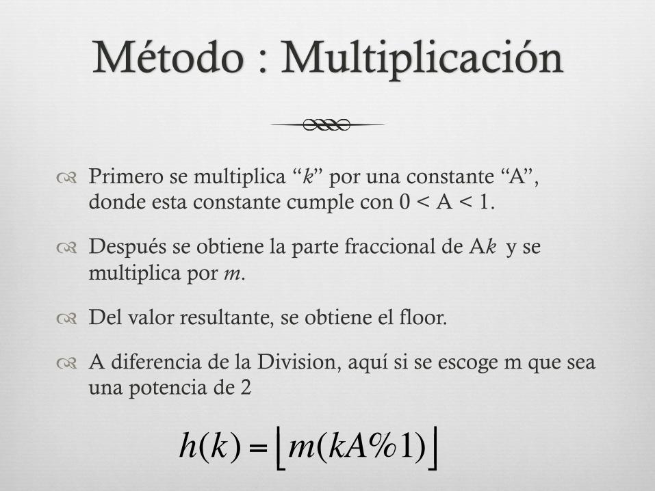
�  Primero se multiplica “k” por una constante “A”, donde esta constante cumple con 0 < A < 1.

�  Después se obtiene la parte fraccional de Ak y se multiplica por m.

�  Del valor resultante, se obtiene el floor.

�  A diferencia de la Division, aquí si se escoge m que sea una potencia de 2

h(k) = m(kA%1)!" #$

Universal Hashing

Selección aleatoria de funciones de Hash

Universal Hashing

�  Se intenta escoger de forma aleatoria una función de una lista finita de funciones de hash existentes, independientemente del valor de la llave.

�  Se dice que “H” es una colección finita de funciones de Hash que apunta a un Universo “U” de llaves.

�  Se dice que la el universo es “Universal” si para cada par distinto de llaves, h(k) = h(l) existe como máximo la posibilidad de colisión de 1/m.

�  La idea del Univesal Hashing reside en evitar que un proceso o persona mal intencionada decida forzar colisiones sobre un slot especifico.

�  Universal Class, es la clase que contiene las funciones y decide cual se va a utilizar para cada llave…

Universal Class

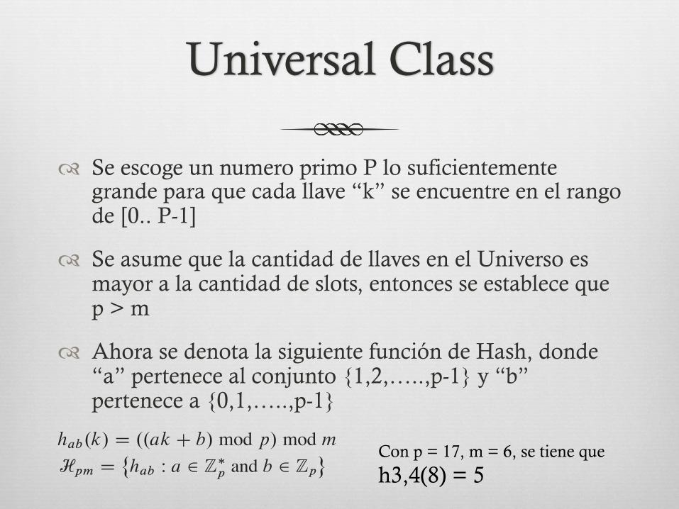
�  Se escoge un numero primo P lo suficientemente grande para que cada llave “k” se encuentre en el rango de [0.. P-1]

�  Se asume que la cantidad de llaves en el Universo es mayor a la cantidad de slots, entonces se establece que p > m

�  Ahora se denota la siguiente función de Hash, donde “a” pertenece al conjunto {1,2,…..,p-1} y “b” pertenece a {0,1,…..,p-1}

11.3 Hash functions 267

expectation, therefore, the expected time for the entire sequence of n operationsis O.n/. Since each operation takes !.1/ time, the ‚.n/ bound follows.

Designing a universal class of hash functionsIt is quite easy to design a universal class of hash functions, as a little numbertheory will help us prove. You may wish to consult Chapter 31 first if you areunfamiliar with number theory.

We begin by choosing a prime number p large enough so that every possiblekey k is in the range 0 to p ! 1, inclusive. Let Zp denote the set f0; 1; : : : ; p ! 1g,and let Z!

p denote the set f1; 2; : : : ; p ! 1g. Since p is prime, we can solve equa-tions modulo p with the methods given in Chapter 31. Because we assume that thesize of the universe of keys is greater than the number of slots in the hash table, wehave p > m.

We now define the hash function hab for any a 2 Z!p and any b 2 Zp using a

linear transformation followed by reductions modulo p and then modulo m:hab.k/ D ..ak C b/ mod p/ mod m : (11.3)For example, with p D 17 and m D 6, we have h3;4.8/ D 5. The family of allsuch hash functions isHpm D

˚hab W a 2 Z

!p and b 2 Zp

!: (11.4)

Each hash function hab maps Zp to Zm. This class of hash functions has the niceproperty that the size m of the output range is arbitrary—not necessarily prime—afeature which we shall use in Section 11.5. Since we have p ! 1 choices for aand p choices for b, the collection Hpm contains p.p ! 1/ hash functions.

Theorem 11.5The class Hpm of hash functions defined by equations (11.3) and (11.4) is universal.

Proof Consider two distinct keys k and l from Zp, so that k ¤ l . For a givenhash function hab we letr D .ak C b/ mod p ;

s D .al C b/ mod p :

We first note that r ¤ s. Why? Observe thatr ! s " a.k ! l/ .mod p/ :

It follows that r ¤ s because p is prime and both a and .k ! l/ are nonzeromodulo p, and so their product must also be nonzero modulo p by Theorem 31.6.Therefore, when computing any hab 2 Hpm, distinct inputs k and l map to distinct

11.3 Hash functions 267

expectation, therefore, the expected time for the entire sequence of n operationsis O.n/. Since each operation takes !.1/ time, the ‚.n/ bound follows.

Designing a universal class of hash functionsIt is quite easy to design a universal class of hash functions, as a little numbertheory will help us prove. You may wish to consult Chapter 31 first if you areunfamiliar with number theory.

We begin by choosing a prime number p large enough so that every possiblekey k is in the range 0 to p ! 1, inclusive. Let Zp denote the set f0; 1; : : : ; p ! 1g,and let Z!

p denote the set f1; 2; : : : ; p ! 1g. Since p is prime, we can solve equa-tions modulo p with the methods given in Chapter 31. Because we assume that thesize of the universe of keys is greater than the number of slots in the hash table, wehave p > m.

We now define the hash function hab for any a 2 Z!p and any b 2 Zp using a

linear transformation followed by reductions modulo p and then modulo m:hab.k/ D ..ak C b/ mod p/ mod m : (11.3)For example, with p D 17 and m D 6, we have h3;4.8/ D 5. The family of allsuch hash functions isHpm D

˚hab W a 2 Z

!p and b 2 Zp

!: (11.4)

Each hash function hab maps Zp to Zm. This class of hash functions has the niceproperty that the size m of the output range is arbitrary—not necessarily prime—afeature which we shall use in Section 11.5. Since we have p ! 1 choices for aand p choices for b, the collection Hpm contains p.p ! 1/ hash functions.

Theorem 11.5The class Hpm of hash functions defined by equations (11.3) and (11.4) is universal.

Proof Consider two distinct keys k and l from Zp, so that k ¤ l . For a givenhash function hab we letr D .ak C b/ mod p ;

s D .al C b/ mod p :

We first note that r ¤ s. Why? Observe thatr ! s " a.k ! l/ .mod p/ :

It follows that r ¤ s because p is prime and both a and .k ! l/ are nonzeromodulo p, and so their product must also be nonzero modulo p by Theorem 31.6.Therefore, when computing any hab 2 Hpm, distinct inputs k and l map to distinct

Con p = 17, m = 6, se tiene que

h3,4(8) = 5

Open Addressing

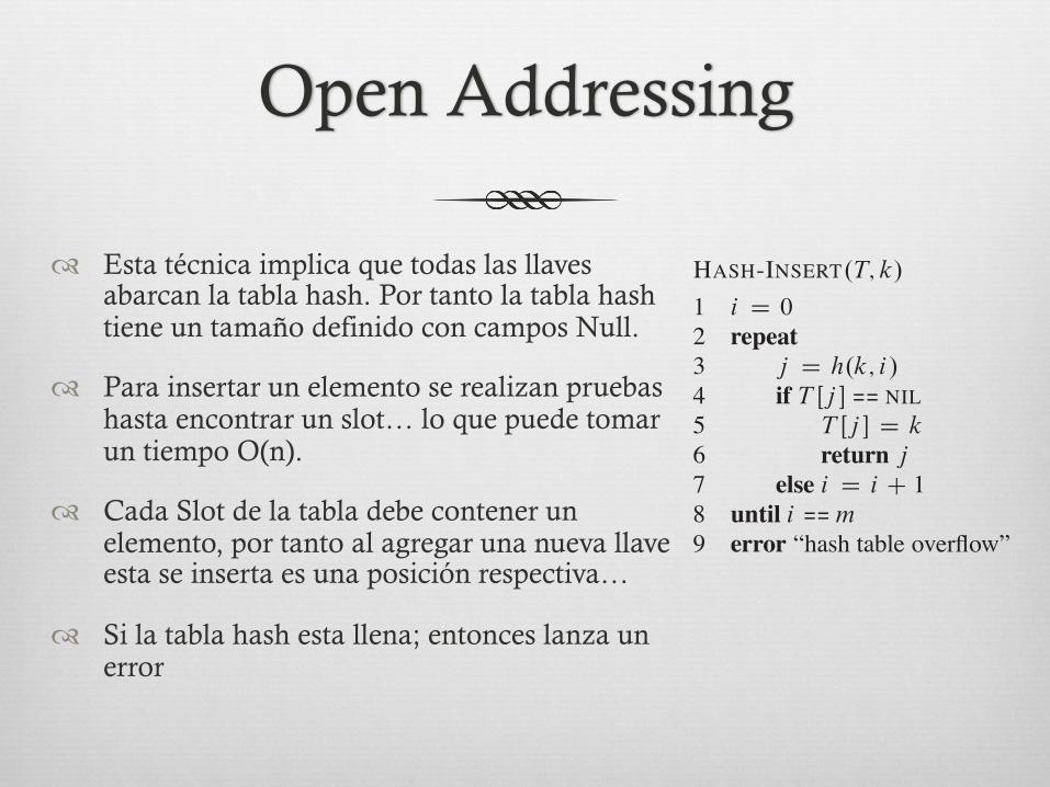
�  Esta técnica implica que todas las llaves abarcan la tabla hash. Por tanto la tabla hash tiene un tamaño definido con campos Null.

�  Para insertar un elemento se realizan pruebas hasta encontrar un slot… lo que puede tomar un tiempo O(n).

�  Cada Slot de la tabla debe contener un elemento, por tanto al agregar una nueva llave esta se inserta es una posición respectiva…

�  Si la tabla hash esta llena; entonces lanza un error


no elements are stored outside the table, unlike in chaining. Thus, in open ad-dressing, the hash table can “fill up” so that no further insertions can be made; oneconsequence is that the load factor ˛ can never exceed 1.

Of course, we could store the linked lists for chaining inside the hash table, inthe otherwise unused hash-table slots (see Exercise 11.2-4), but the advantage ofopen addressing is that it avoids pointers altogether. Instead of following pointers,we compute the sequence of slots to be examined. The extra memory freed by notstoring pointers provides the hash table with a larger number of slots for the sameamount of memory, potentially yielding fewer collisions and faster retrieval.

To perform insertion using open addressing, we successively examine, or probe,the hash table until we find an empty slot in which to put the key. Instead of beingfixed in the order 0; 1; : : : ; m ! 1 (which requires ‚.n/ search time), the sequenceof positions probed depends upon the key being inserted. To determine which slotsto probe, we extend the hash function to include the probe number (starting from 0)as a second input. Thus, the hash function becomesh W U " f0; 1; : : : ; m ! 1g ! f0; 1; : : : ; m ! 1g :

With open addressing, we require that for every key k, the probe sequencehh.k; 0/; h.k; 1/; : : : ; h.k; m ! 1/i

be a permutation of h0;1; : : : ;m!1i, so that every hash-table position is eventuallyconsidered as a slot for a new key as the table fills up. In the following pseudocode,we assume that the elements in the hash table T are keys with no satellite infor-mation; the key k is identical to the element containing key k. Each slot containseither a key or NIL (if the slot is empty). The HASH-INSERT procedure takes asinput a hash table T and a key k. It either returns the slot number where it storeskey k or flags an error because the hash table is already full.

HASH-INSERT.T; k/

1 i D 02 repeat3 j D h.k; i/4 if T Œj ! == NIL5 T Œj ! D k6 return j7 else i D i C 18 until i == m9 error “hash table overflow”

The algorithm for searching for key k probes the same sequence of slots that theinsertion algorithm examined when key k was inserted. Therefore, the search can

Open Addressing

11.4 Open addressing 271

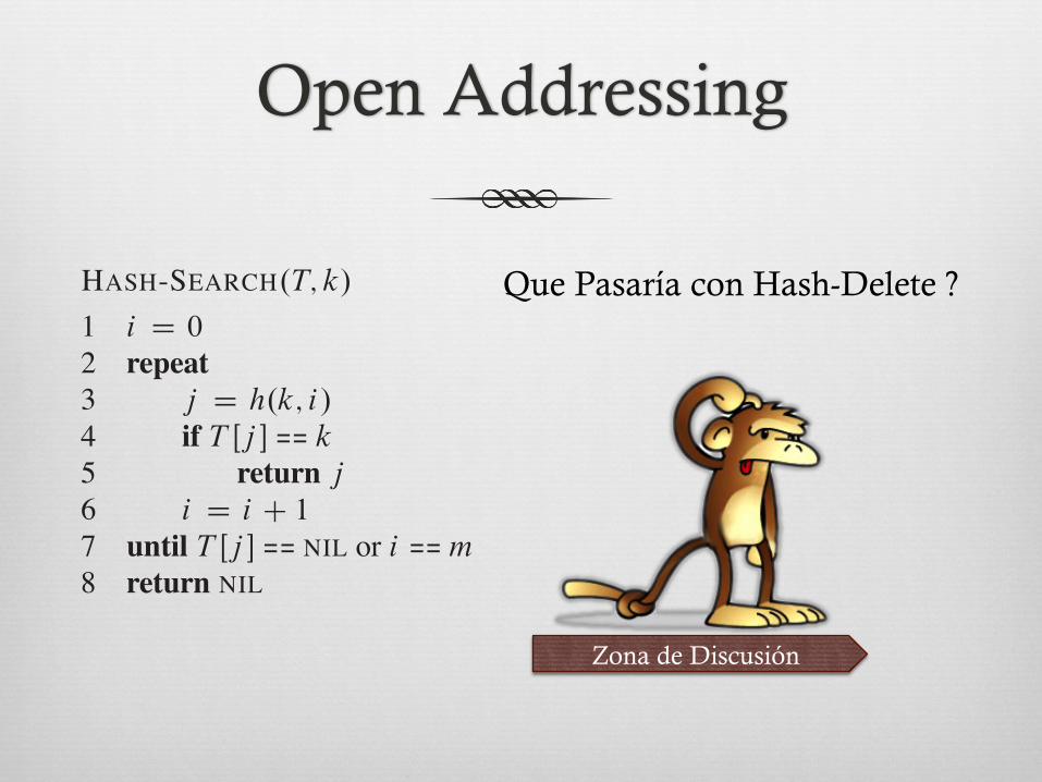
terminate (unsuccessfully) when it finds an empty slot, since k would have beeninserted there and not later in its probe sequence. (This argument assumes that keysare not deleted from the hash table.) The procedure HASH-SEARCH takes as inputa hash table T and a key k, returning j if it finds that slot j contains key k, or NILif key k is not present in table T .

HASH-SEARCH.T; k/

1 i D 02 repeat3 j D h.k; i/4 if T Œj ! == k5 return j6 i D i C 17 until T Œj ! == NIL or i == m8 return NIL

Deletion from an open-address hash table is difficult. When we delete a keyfrom slot i , we cannot simply mark that slot as empty by storing NIL in it. Ifwe did, we might be unable to retrieve any key k during whose insertion we hadprobed slot i and found it occupied. We can solve this problem by marking theslot, storing in it the special value DELETED instead of NIL. We would then modifythe procedure HASH-INSERT to treat such a slot as if it were empty so that we caninsert a new key there. We do not need to modify HASH-SEARCH, since it will passover DELETED values while searching. When we use the special value DELETED,however, search times no longer depend on the load factor ˛, and for this reasonchaining is more commonly selected as a collision resolution technique when keysmust be deleted.

In our analysis, we assume uniform hashing: the probe sequence of each keyis equally likely to be any of the m" permutations of h0; 1; : : : ; m ! 1i. Uni-form hashing generalizes the notion of simple uniform hashing defined earlier to ahash function that produces not just a single number, but a whole probe sequence.True uniform hashing is difficult to implement, however, and in practice suitableapproximations (such as double hashing, defined below) are used.

We will examine three commonly used techniques to compute the probe se-quences required for open addressing: linear probing, quadratic probing, and dou-ble hashing. These techniques all guarantee that hh.k; 0/; h.k; 1/; : : : ; h.k;m ! 1/iis a permutation of h0; 1; : : : ; m ! 1i for each key k. None of these techniques ful-fills the assumption of uniform hashing, however, since none of them is capable ofgenerating more than m2 different probe sequences (instead of the m" that uniformhashing requires). Double hashing has the greatest number of probe sequences and,as one might expect, seems to give the best results.

Que Pasaría con Hash-Delete ?

Zona de Discusión

Probes – Open Addressing

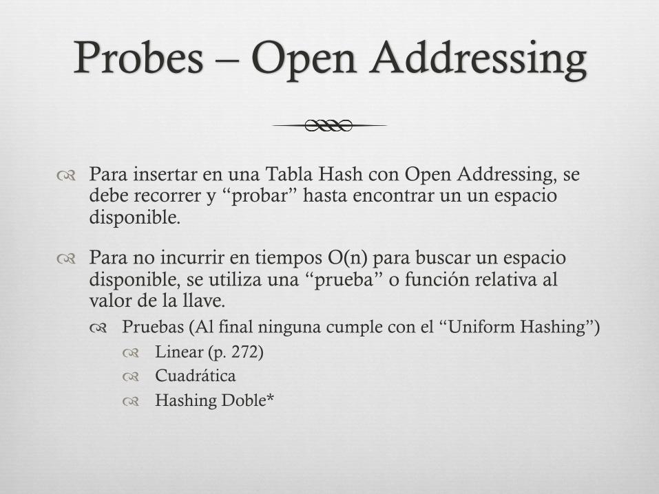
�  Para insertar en una Tabla Hash con Open Addressing, se debe recorrer y “probar” hasta encontrar un un espacio disponible.

�  Para no incurrir en tiempos O(n) para buscar un espacio disponible, se utiliza una “prueba” o función relativa al valor de la llave. �  Pruebas (Al final ninguna cumple con el “Uniform Hashing”)

�  Linear (p. 272) �  Cuadrática

�  Hashing Doble*

Linear Probing

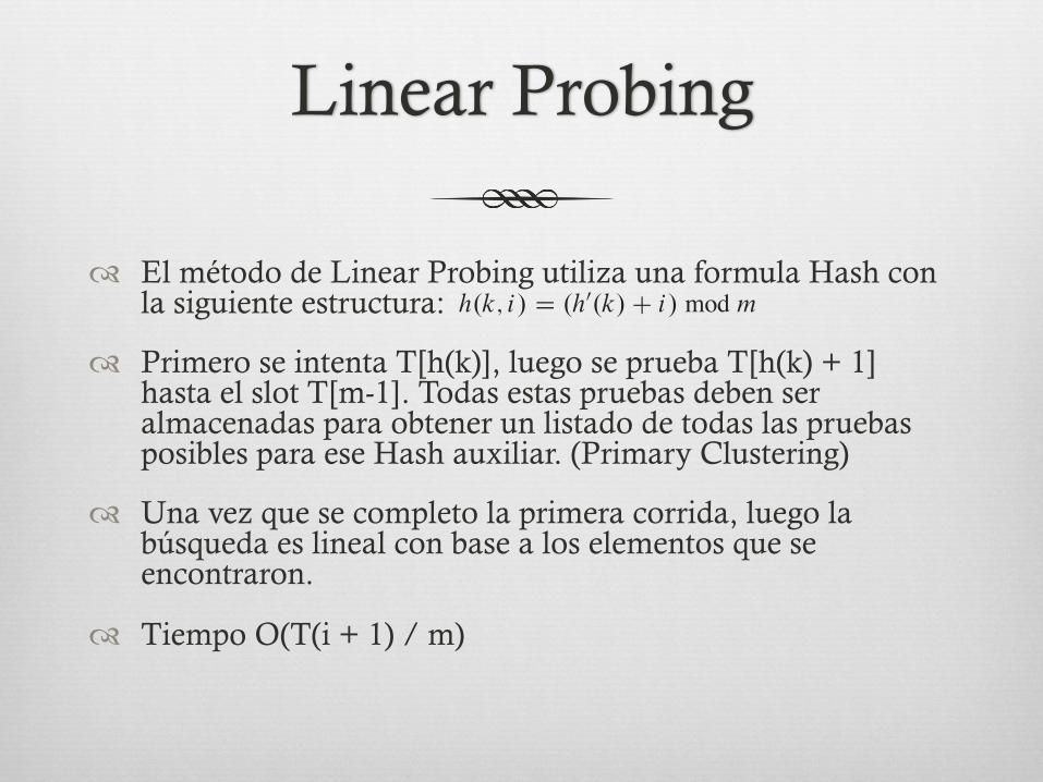
�  El método de Linear Probing utiliza una formula Hash con la siguiente estructura:

�  Primero se intenta T[h(k)], luego se prueba T[h(k) + 1] hasta el slot T[m-1]. Todas estas pruebas deben ser almacenadas para obtener un listado de todas las pruebas posibles para ese Hash auxiliar. (Primary Clustering)

�  Una vez que se completo la primera corrida, luego la búsqueda es lineal con base a los elementos que se encontraron.

�  Tiempo O(T(i + 1) / m)


Linear probingGiven an ordinary hash function h0 W U ! f0; 1; : : : ; m ! 1g, which we refer to asan auxiliary hash function, the method of linear probing uses the hash functionh.k; i/ D .h0.k/C i/ mod m

for i D 0; 1; : : : ; m ! 1. Given key k, we first probe T Œh0.k/!, i.e., the slot givenby the auxiliary hash function. We next probe slot T Œh0.k/ C 1!, and so on up toslot T Œm ! 1!. Then we wrap around to slots T Œ0!; T Œ1!; : : : until we finally probeslot T Œh0.k/ ! 1!. Because the initial probe determines the entire probe sequence,there are only m distinct probe sequences.

Linear probing is easy to implement, but it suffers from a problem known asprimary clustering. Long runs of occupied slots build up, increasing the averagesearch time. Clusters arise because an empty slot preceded by i full slots gets fillednext with probability .i C 1/=m. Long runs of occupied slots tend to get longer,and the average search time increases.

Quadratic probingQuadratic probing uses a hash function of the formh.k; i/ D .h0.k/C c1i C c2i2/ mod m ; (11.5)where h0 is an auxiliary hash function, c1 and c2 are positive auxiliary constants,and i D 0; 1; : : : ; m ! 1. The initial position probed is T Œh0.k/!; later positionsprobed are offset by amounts that depend in a quadratic manner on the probe num-ber i . This method works much better than linear probing, but to make full use ofthe hash table, the values of c1, c2, and m are constrained. Problem 11-3 showsone way to select these parameters. Also, if two keys have the same initial probeposition, then their probe sequences are the same, since h.k1; 0/ D h.k2; 0/ im-plies h.k1; i/ D h.k2; i/. This property leads to a milder form of clustering, calledsecondary clustering. As in linear probing, the initial probe determines the entiresequence, and so only m distinct probe sequences are used.

Double hashingDouble hashing offers one of the best methods available for open addressing be-cause the permutations produced have many of the characteristics of randomlychosen permutations. Double hashing uses a hash function of the formh.k; i/ D .h1.k/C ih2.k// mod m ;

where both h1 and h2 are auxiliary hash functions. The initial probe goes to posi-tion T Œh1.k/!; successive probe positions are offset from previous positions by the

Quadratic Probing

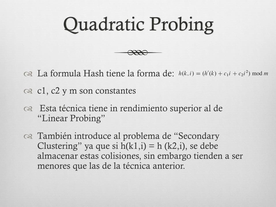
�  La formula Hash tiene la forma de:

�  c1, c2 y m son constantes

�  Esta técnica tiene in rendimiento superior al de “Linear Probing”

�  También introduce al problema de “Secondary Clustering” ya que si h(k1,i) = h (k2,i), se debe almacenar estas colisiones, sin embargo tienden a ser menores que las de la técnica anterior.








Double Hashing

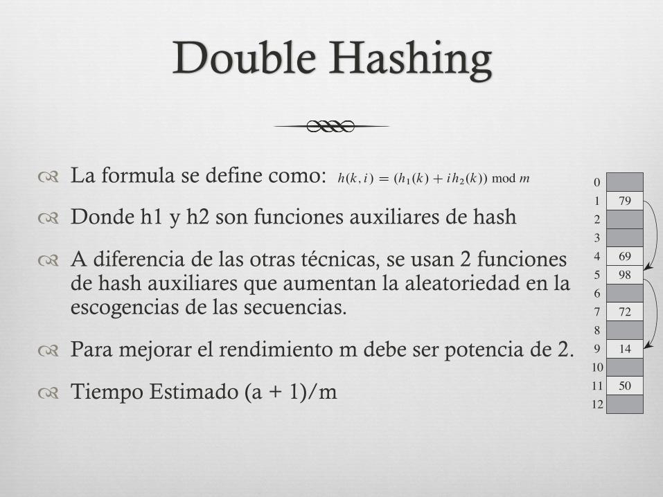
�  La formula se define como:

�  Donde h1 y h2 son funciones auxiliares de hash

�  A diferencia de las otras técnicas, se usan 2 funciones de hash auxiliares que aumentan la aleatoriedad en la escogencias de las secuencias.

�  Para mejorar el rendimiento m debe ser potencia de 2.

�  Tiempo Estimado (a + 1)/m








11.4 Open addressing 273

0123456789101112

79

6998

72

14

50

Figure 11.5 Insertion by double hashing. Here we have a hash table of size 13 with h1.k/ Dk mod 13 and h2.k/ D 1C .k mod 11/. Since 14 ! 1 .mod 13/ and 14 ! 3 .mod 11/, we insertthe key 14 into empty slot 9, after examining slots 1 and 5 and finding them to be occupied.

amount h2.k/, modulo m. Thus, unlike the case of linear or quadratic probing, theprobe sequence here depends in two ways upon the key k, since the initial probeposition, the offset, or both, may vary. Figure 11.5 gives an example of insertionby double hashing.

The value h2.k/ must be relatively prime to the hash-table size m for the entirehash table to be searched. (See Exercise 11.4-4.) A convenient way to ensure thiscondition is to let m be a power of 2 and to design h2 so that it always produces anodd number. Another way is to let m be prime and to design h2 so that it alwaysreturns a positive integer less than m. For example, we could choose m prime andleth1.k/ D k mod m ;

h2.k/ D 1C .k mod m0/ ;

where m0 is chosen to be slightly less than m (say, m " 1). For example, ifk D 123456, m D 701, and m0 D 700, we have h1.k/ D 80 and h2.k/ D 257, sothat we first probe position 80, and then we examine every 257th slot (modulo m)until we find the key or have examined every slot.

When m is prime or a power of 2, double hashing improves over linear or qua-dratic probing in that ‚.m2/ probe sequences are used, rather than ‚.m/, sinceeach possible .h1.k/; h2.k// pair yields a distinct probe sequence. As a result, for

Tarea Hashing

�  Que es Perfect Hashing (a diferencia del approach tradicional con Colission + Chaining)?

�  Que relación tiene con Universal Hashing?

�  Como se asegura el tiempo O(1)?

�  Bajo que escenarios se puede implementar Perfect Hashing?

�  Que tamaño debe ser “m” para garantizar esto?

Sección 11.5 MIT

Education

Hashing