Controller Principles

19AEI-406.9

29AEI-406.9

Control System parameters

Control system parameters are

• Error

• Controller output

• Control lag

• Dead time

• Cycling

39AEI-406.9

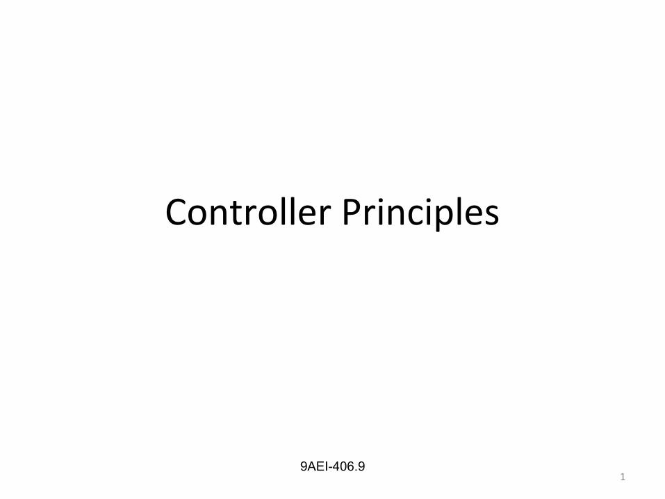
C F.C.E P

F.B

+-

S.P

C.V

e m

Block Diagram of Process Control Loop

49AEI-406.9

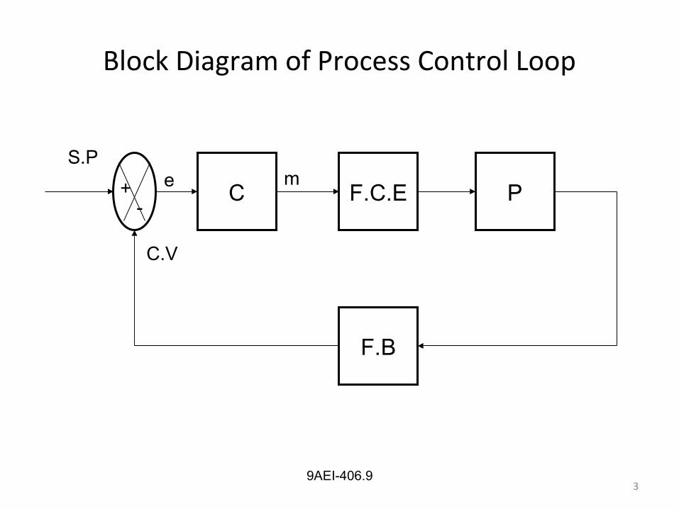
The deviation of controlled variable from set point is

called error

It is given by

e = r – b

Where

b = measured value

r = set point

e = error

Error

+ -r

b

e = r-b

Error detector

59AEI-406.9

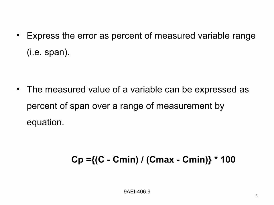
• Express the error as percent of measured variable range

(i.e. span).

• The measured value of a variable can be expressed as

percent of span over a range of measurement by

equation.

Cp ={(C - Cmin) / (Cmax - Cmin)} * 100

69AEI-406.9

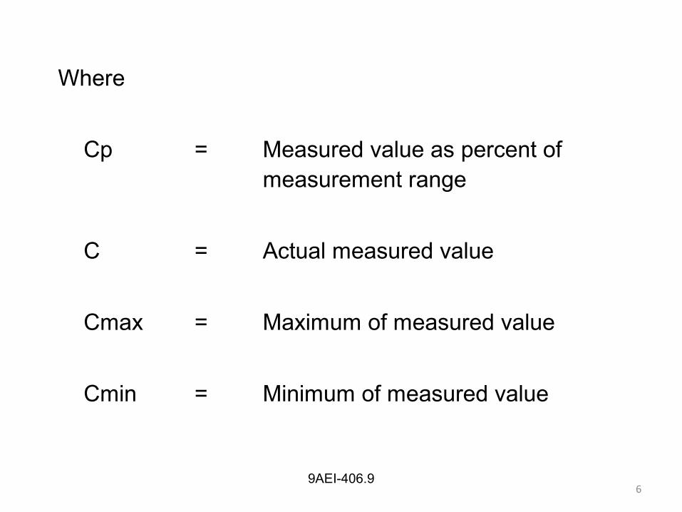
Where

Cp = Measured value as percent of measurement range

C = Actual measured value

Cmax = Maximum of measured value

Cmin = Minimum of measured value

79AEI-406.9

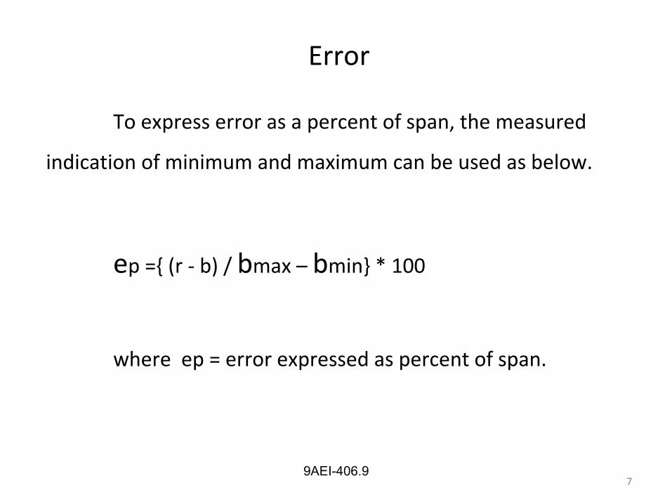
Error

To express error as a percent of span, the measured

indication of minimum and maximum can be used as below.

ep ={ (r - b) / bmax – bmin} * 100

where ep = error expressed as percent of span.

89AEI-406.9

Variable range

• The variable under control has a range of values within which

control is maintained.

• This range can be expressed as the minimum and maximum

value of the variable or the nominal value plus and minus the

spread about this nominal.

• If a standard 4-20mA signal transmission is employed, then

4mA represents the minimum value of the variable and 20mA

the maximum.

8

99AEI-406.9

Control parameter range

• The controller output range is the translation of output to the

range of possible values of the final control element.

• This range also is expressed as the 4-20mA standard signal

again with the minimum and maximum effects in terms of the

minimum and maximum current.

9

109AEI-406.9

Control lag

• The control system also has a lag associated with its operation

that must be compared to the process lag.

• When a controlled variable experiences a sudden change, the

process-control loop reacts by outputting a command to the

final control element to adopt a new value to compensate for

the detected change.

119AEI-406.9

Example

129AEI-406.9

Control lag

• “Control lag refers to the time for the process-control loop

to make necessary adjustments to the final control element”.

• If a sudden change in liquid temperature occurs, it

requires some finite time for the control system to physically

actuate the steam control value.

12

139AEI-406.9

Dead time

• Time variable associated with process control is both a

function of the process-control system and the process.

• “This is the elapsed time between the instant deviation

(error) occurs and the correction action first occurs”.

149AEI-406.9

• An example of dead time occurs in the control of a

chemical reaction by varying reactant flow rate through a

long pipe.

• When a deviation is detected, a control system quickly

changes a value setting to adjust flow rate. but if pipe is

quite long, there is a period of time during which no

effect is felt in the reaction vessel.

159AEI-406.9

Dead Time

• This is the time required for the new flow rate to move

down the length of the pipe.

• Such dead times can have a very profound effect on the

performance of control operations on a process.

15

169AEI-406.9

Cycling

• Cycling the behavior of the dynamic variable error under various modes of control.

• One of the most important modes is an oscillation of the error about zero.

• This means the variable is cycling above and below the set point value.

• Such cycling may continue indefinitely, in which case we have ‘steady-state cycling’.

16

179AEI-406.9

Cycling

• Here interested in both the peak amplitude of the ‘error

‘and the ‘period of the oscillation’.

• If the cycling amplitude decays to zero, however, we

have a cyclic transient error.

• Here we are interested in the ‘initial error’, the period of

the cyclic oscillation, and ‘decay time’ for the error to reach

zero.

Controller Modes

9AEI-406.1018

9AEI-406.1019

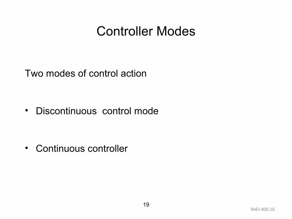
Controller Modes

Two modes of control action

• Discontinuous control mode

• Continuous controller

9AEI-406.1020

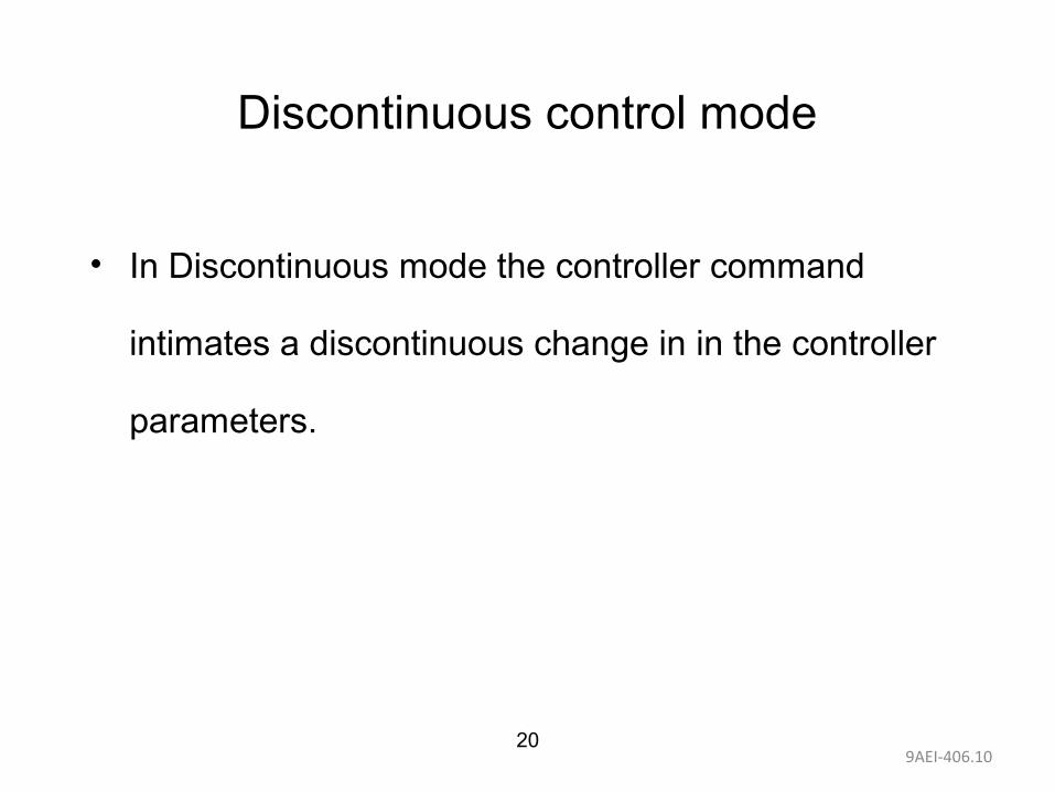
Discontinuous control mode

• In Discontinuous mode the controller command

intimates a discontinuous change in in the controller

parameters.

9AEI-406.1021

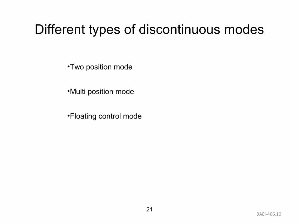
Different types of discontinuous modes

•Two position mode

•Multi position mode

•Floating control mode

9AEI-406.1022

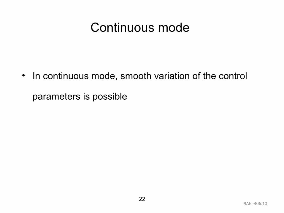
Continuous mode

• In continuous mode, smooth variation of the control

parameters is possible

9AEI-406.1023

Different types of continuous modes

• Proportional controller (P)

• Integral controller (I)

• Derivative controller (D)

• Composite control modes

9AEI-406.1024

Composite controller modes

Composite controller modes combine the continuous control modes

Proportional – Integral (PI)

Proportional – Derivative (PD)

Proportional – Integral – Derivative (PID)

9AEI-406.1025

Control actions

• The error that result from the measurement of the

controlled variable may be positive or negative.

Types of control action

• Direct action

• Reverse action

9AEI-406.1026

Direct action

• A controller is said to be operated with direct action when

an increasing value of the controller output.

• Example level control system.

• If the level rises (controlled variable increases) the control

output should increase to open the valve more to keep the

level under control.

9AEI-406.1027

Reverse action

• A control is said to be operating with reverse action when

an increasing value of the controlled variable causes a

decreasing value of the controller output.

• Example a simple temperature control of furnace with

fuel as heat energy.

• If the temperature increases, the control output should

decrease to close the valve for decreasing the fuel input

to bring the temperature under control

289AEI-406.11 & 12

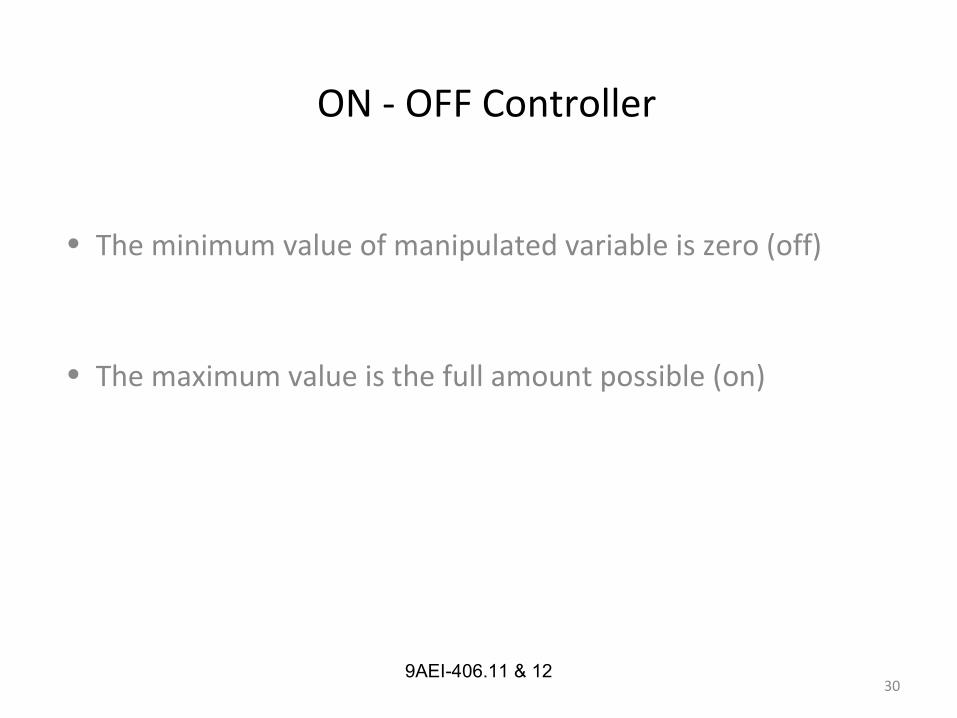
ON - OFF Controller

• Two position control is a position type of a controller action in

which manipulated variable is quickly changed to either

maximum (or) minimum value depending upon whether the

controlled variable is greater or less than the set point

• Two position control mode is also called ON – OFF control

mode

28

299AEI-406.11 & 12

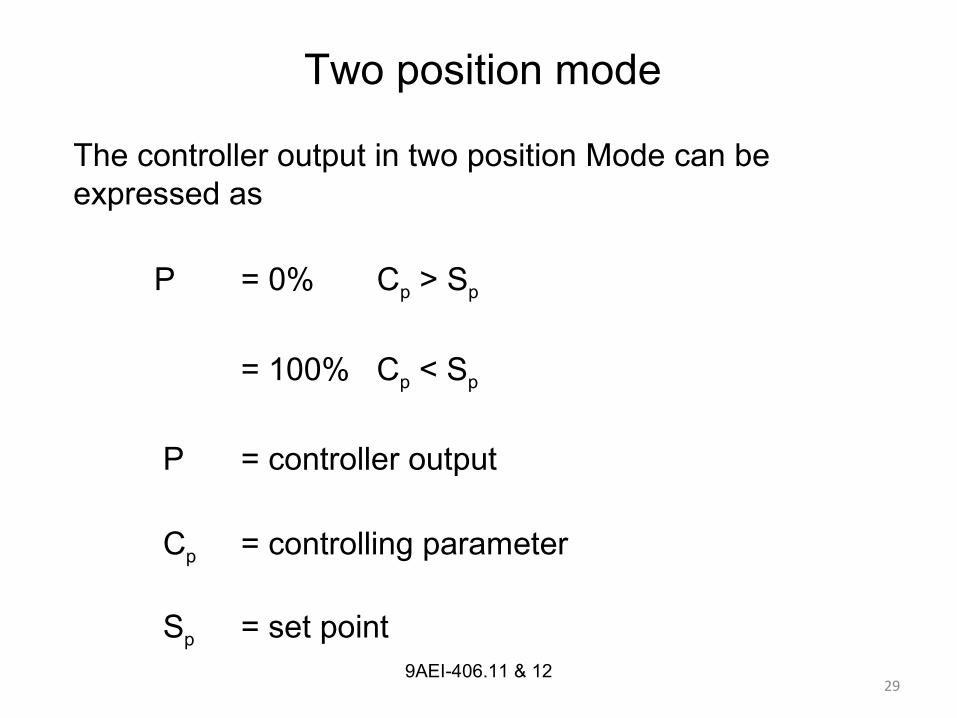
P = 0% Cp > Sp

= 100% Cp < Sp

P = controller output

Cp = controlling parameter

Sp = set point

The controller output in two position Mode can be expressed as

Two position mode

309AEI-406.11 & 12

ON - OFF Controller

• The minimum value of manipulated variable is zero (off)

• The maximum value is the full amount possible (on)

319AEI-406.11 & 12 31

329AEI-406.11 & 12

ON - OFF Controller

The relation ship shows that

• When the measured value is less than set point, full control

output result.

• When is more than set point, the controller output is zero.

339AEI-406.11 & 12

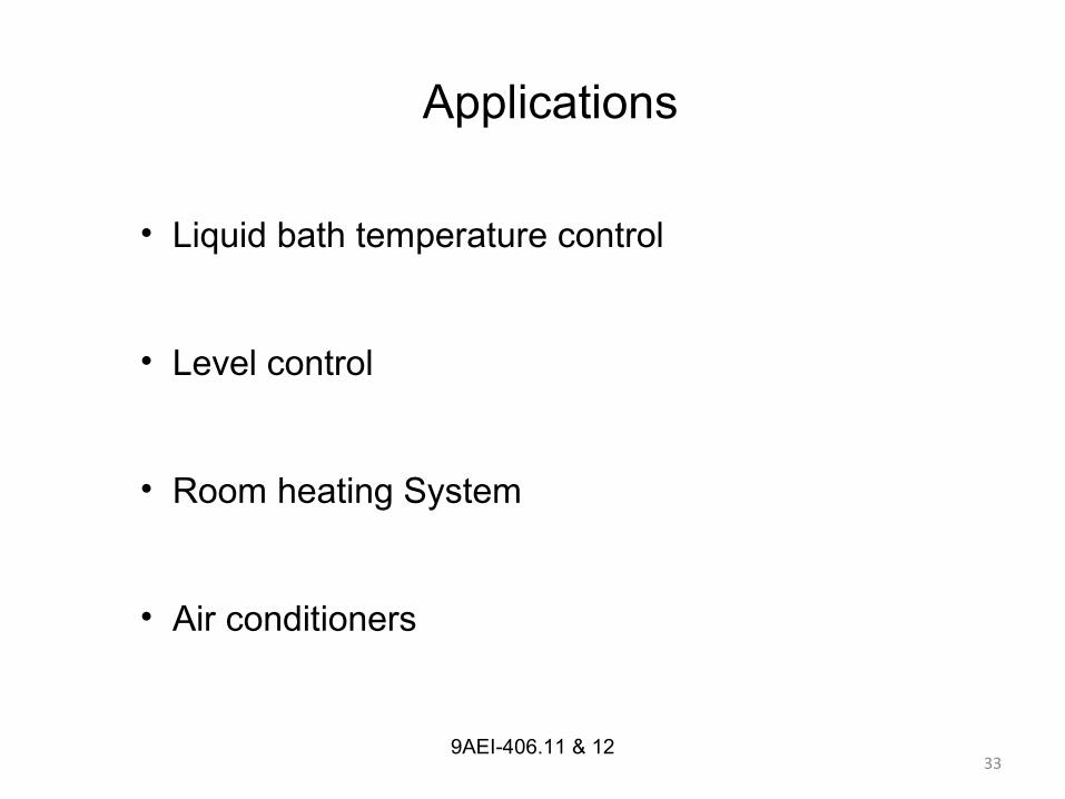
• Liquid bath temperature control

• Level control

• Room heating System

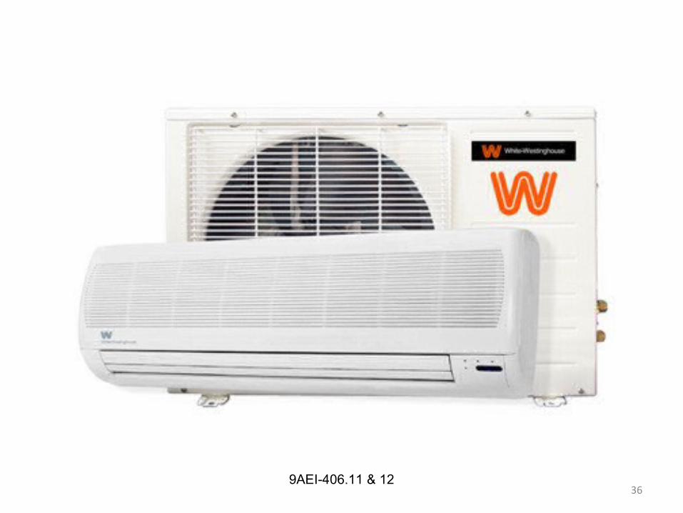
• Air conditioners

Applications

349AEI-406.11 & 12

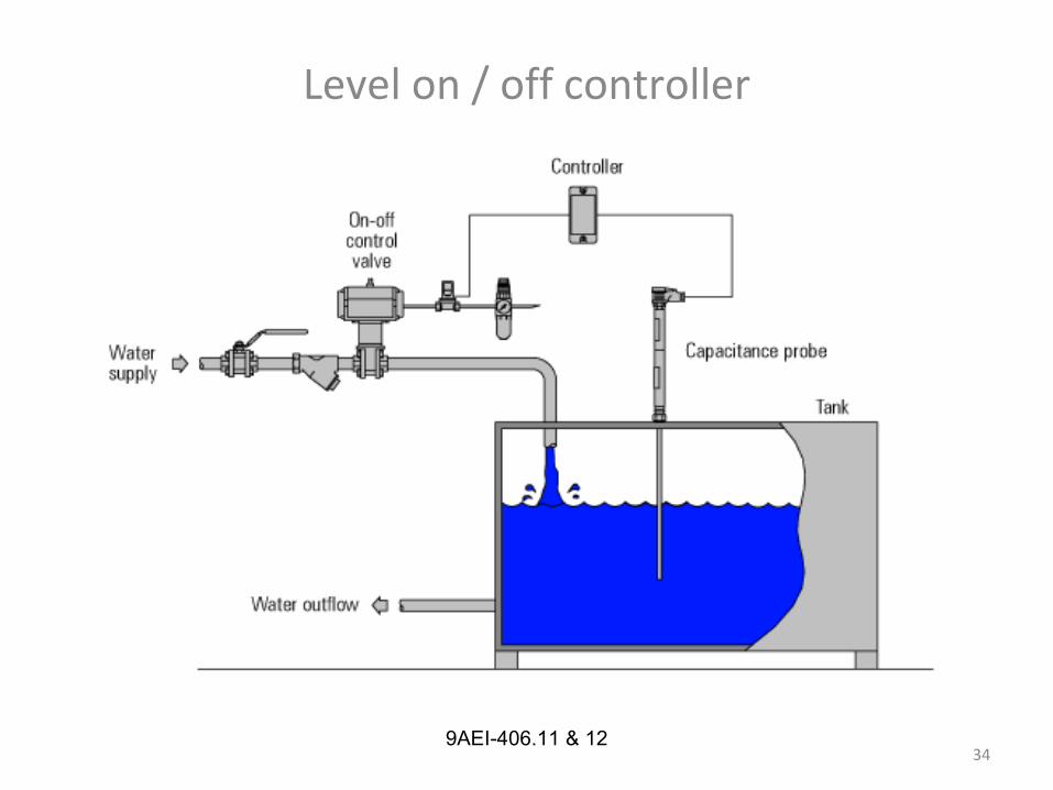
Level on / off controller

359AEI-406.11 & 12

369AEI-406.11 & 12

379AEI-406.11 & 12

Advantages

• Simplest and cheapest.

• Two position controller is suitable for system with slow

process rates.

389AEI-406.11 & 12

Disadvantages

• Over shoot and Under shoot resultant continuous oscillation

• Neutral zone

399AEI-406.11 & 12

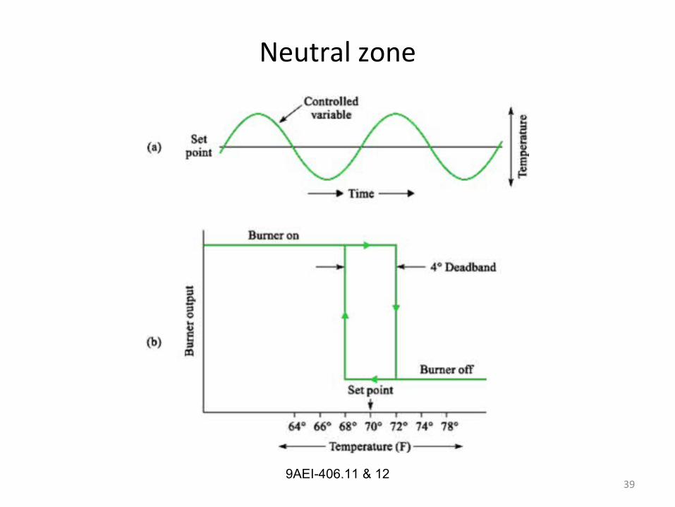
Neutral zone

409AEI-406.11 & 12

Neutral zone

• In practical implementation of the two position controller

• There is an overlap as ep increases through zero or

decreases through zero

• In this span, no change in controller output occurs fig.1

419AEI-406.11 & 12

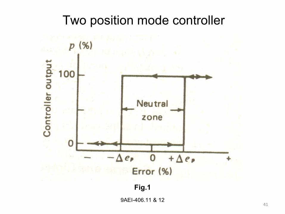
Two position mode controller

Fig.1

429AEI-406.11 & 12

• The controller output changes to 100% when the error

changes above Δ ep

• The controller output changes to 0% when the error

changes below Δ ep

Neutral zone

439AEI-406.11 & 12

Neutral zone

• The range 2 Δ ep is called as the neutral zone

• This is also called as differential gap

• This is purposefully designed above a certain level

• This prevents excessive cycling

• This is a desirable Hysteresis in a system

9AEI-406.1344

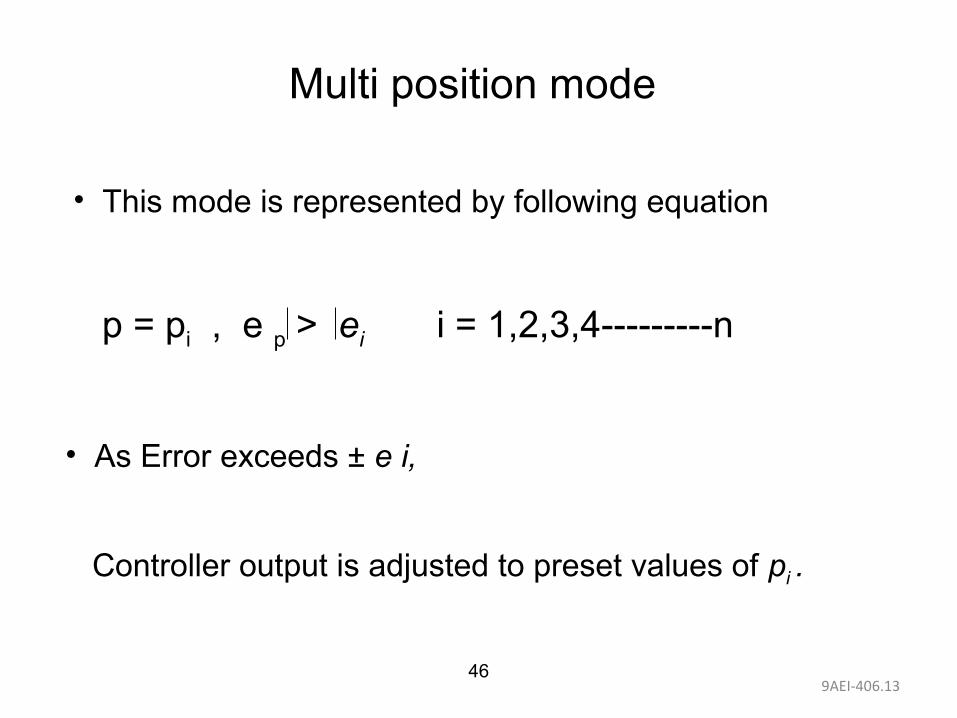
Multi position mode

• A logical extension of two position control is to provide

several inter mediate rather than only two settings of the

controller output.

• Multi position mode is used to reduce the cycling behavior

and over shoot & undershoot inherent in two position

mode.

9AEI-406.1345

• A three position mode is one in which the manipulated

variable takes one of three value.

• High

• Medium

• Low

9AEI-406.1346

Multi position mode

p = pi , e p > ei i = 1,2,3,4---------n

• As Error exceeds ± e i,

Controller output is adjusted to preset values of pi .

• This mode is represented by following equation

9AEI-406.1347

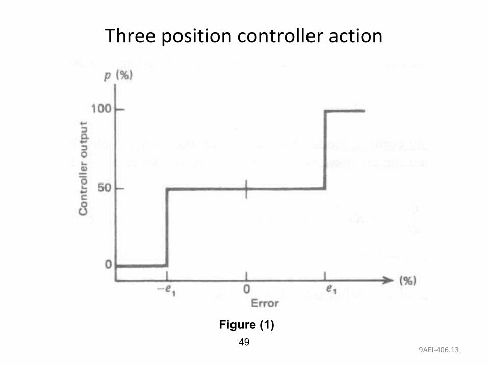
• Three - position controller is best example for multi

position controller

• The controller output in 3- position controller is

P = 100 % e p > e2

= 50 % - e1< e p < e2

= 0 % ep < - e1

Example for multi position controller

9AEI-406.1348

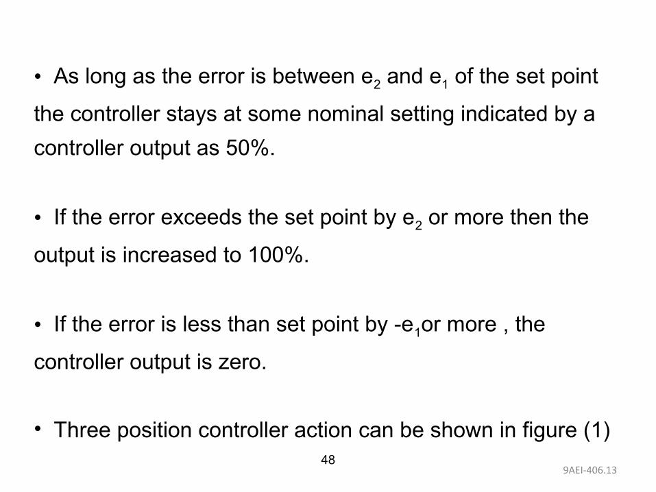
• As long as the error is between e2 and e1 of the set point

the controller stays at some nominal setting indicated by a

controller output as 50%.

• If the error exceeds the set point by e2 or more then the

output is increased to 100%.

• If the error is less than set point by -e1or more , the

controller output is zero.

• Three position controller action can be shown in figure (1)

9AEI-406.1349

Three position controller action

Figure (1)

9AEI-406.1350

Advantages

• Reduce the cycling behavior

• Reduce the overshoots

• Reduce the undershoots

9AEI-406.1351

Disadvantages

• It requires more complicated final control element (It

requires more than two settings).

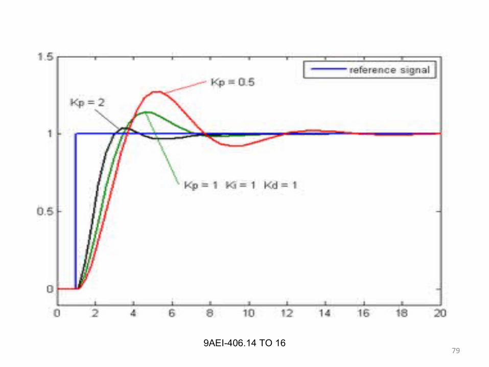
529AEI-406.14 TO 16

Proportional control

• A proportional control system is a type of linear feedback

control system.

• Two classic mechanical examples are the toilet bowl float

proportioning valve and the fly-ball governor.

539AEI-406.14 TO 16 53

549AEI-406.14 TO 16

Proportional controller

• Proportional action is a mode of controller action in

which there is a continuous linear relation exist between the

controller and error.

54

559AEI-406.14 TO 16

• Proportion action is mode of control action In which there is

a continuous linear relation between value of the deviation

and manipulated variable.

• The action of control variable is repeated and amplified in

the action of the control element.

55

569AEI-406.14 TO 16

Proportional controller

Proportional controller also called

• Correspondence controller

• Droop control

• Modulating controller

579AEI-406.14 TO 16

• In the proportional control algorithm, the controller output is

proportional to the error signal, which is the difference

between the set point and the process variable.

• In other words, the output of a proportional controller is the

multiplication product of the error signal and the proportional

gain.

589AEI-406.14 TO 16

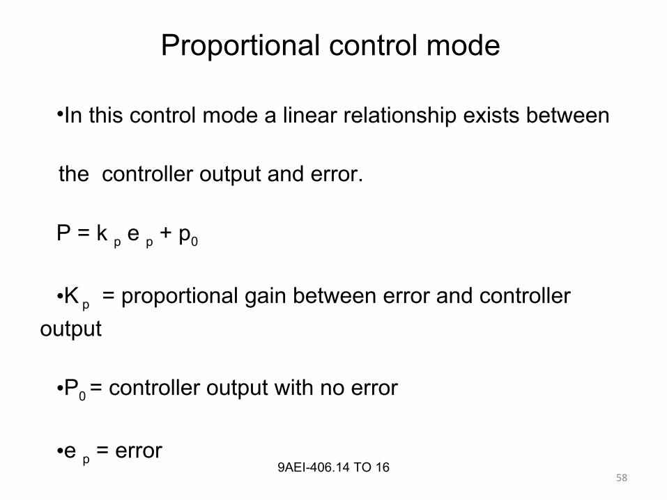
•In this control mode a linear relationship exists between

the controller output and error.

P = k p e p + p0

•K p = proportional gain between error and controller

output

•P0 = controller output with no error

•e p = error

•p= controller output.

Proportional control mode

599AEI-406.14 TO 16

Proportional Band (PB)

•It is defined as the range of error to cover 0% to 100%

controlled output.

609AEI-406.14 TO 16 60

•PB can be expressed by the equation

PB =

K p = proportional gain

PB = proportional band

• PB is dependent on gain. High gain means large

response to an error

100

Kp

619AEI-406.14 TO 16 61

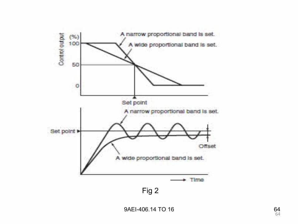
Fig.1

629AEI-406.14 TO 16

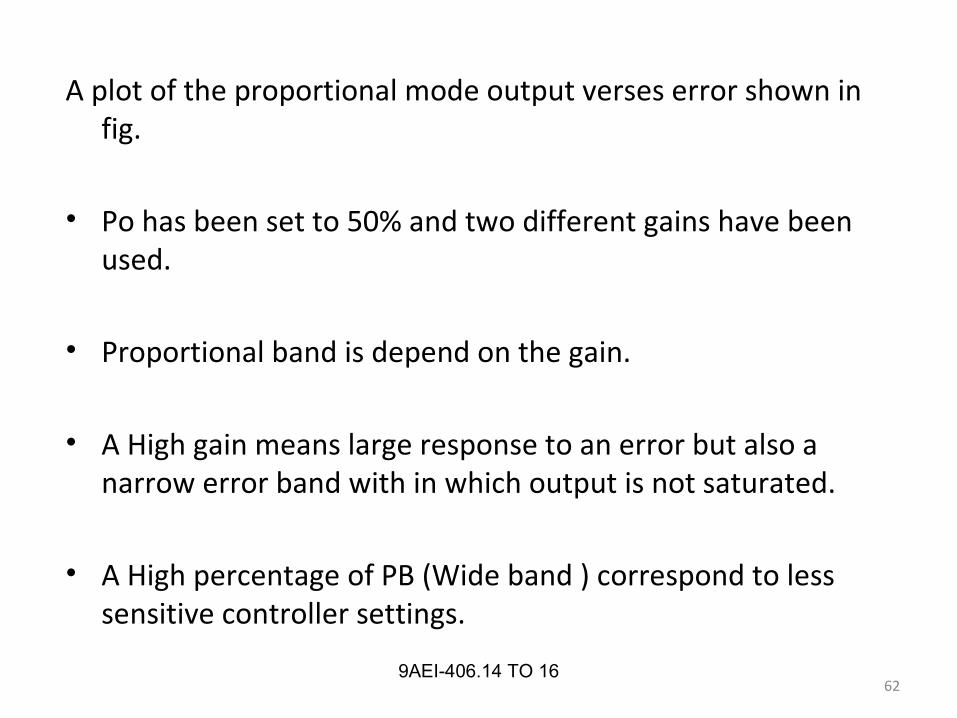
A plot of the proportional mode output verses error shown in fig.

• Po has been set to 50% and two different gains have been used.

• Proportional band is depend on the gain.

• A High gain means large response to an error but also a narrow error band with in which output is not saturated.

• A High percentage of PB (Wide band ) correspond to less sensitive controller settings.

639AEI-406.14 TO 16 63

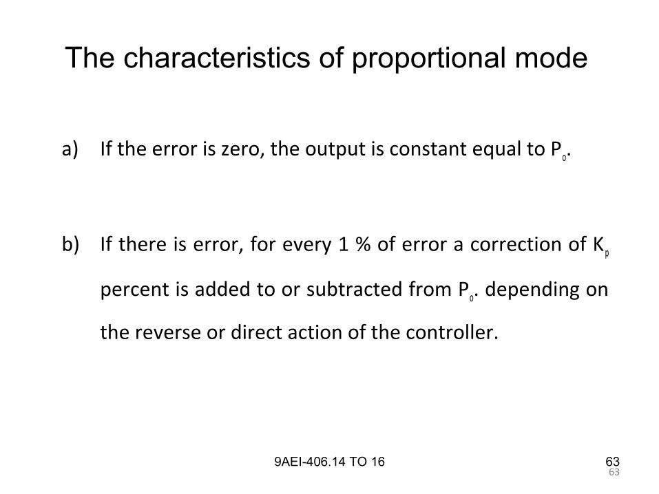
a) If the error is zero, the output is constant equal to Po.

b) If there is error, for every 1 % of error a correction of Kp

percent is added to or subtracted from Po. depending on

the reverse or direct action of the controller.

The characteristics of proportional mode

649AEI-406.14 TO 16 64

Fig 2

659AEI-406.14 TO 16 65

Fig.3

669AEI-406.14 TO 16

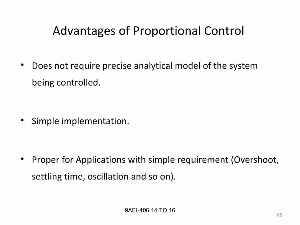
Advantages of Proportional Control

• Does not require precise analytical model of the system

being controlled.

• Simple implementation.

• Proper for Applications with simple requirement (Overshoot,

settling time, oscillation and so on).

679AEI-406.14 TO 16

Disadvantages of Proportional Control

• Inaccurate model may cause steady-state error nonzero

• Disturbance input is non zero

• Reference input is non zero

• Noise input

• Inaccurate model may cause oscillations.

67

689AEI-406.14 TO 16

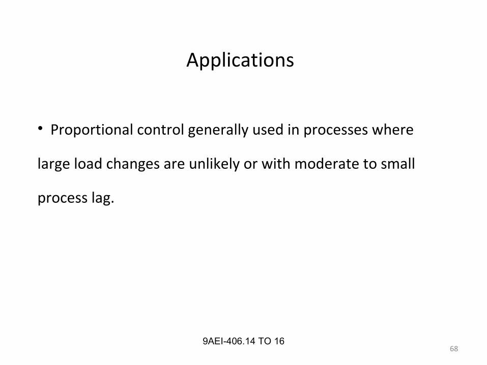
Applications

• Proportional control generally used in processes where

large load changes are unlikely or with moderate to small

process lag.

699AEI-406.14 TO 16

• Offset is a permanent ‘residual error’ in the operating

point of the controlled variable when load change occurs

• Offset can be minimized by a larger value of Kp

(proportional gain).

OFFSET

709AEI-406.14 TO 16

Fig.4

719AEI-406.14 TO 16

OFFSET

• consider a system under nominal load with the controller at

50%and the error zero as shown in Fig 2.

• If the transient error occurs the system respond by changing

controller out put in correspondence with the transient to

effect return to zero error

729AEI-406.14 TO 16

• If the transient error occurs the system respond by changing controller out put in correspondence with the transient to effect return to zero error.

• A load change error that requires a permanent change in controller output to produce the zero error state.

• One to one correspondence exist between controller out put and error , it is clear that a new zero controller out put never be achieved.

• The system produces a small permanent offset in reaching a compromise position of controller output under new load

739AEI-406.14 TO 16

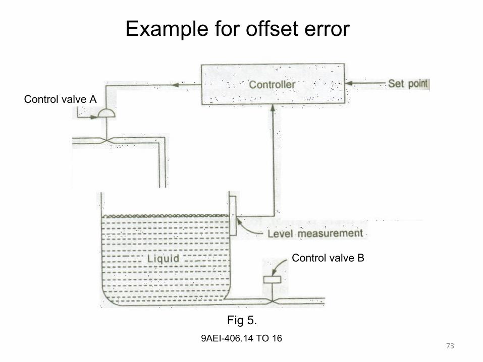
Example for offset error

Fig 5.

Control valve A

Control valve B

749AEI-406.14 TO 16

• Consider the proportional mode level control system as

shown in fig 1.

• For understanding the offset error some of the numerical

values regarding proportional controller output and gain

values are assumed.

759AEI-406.14 TO 16

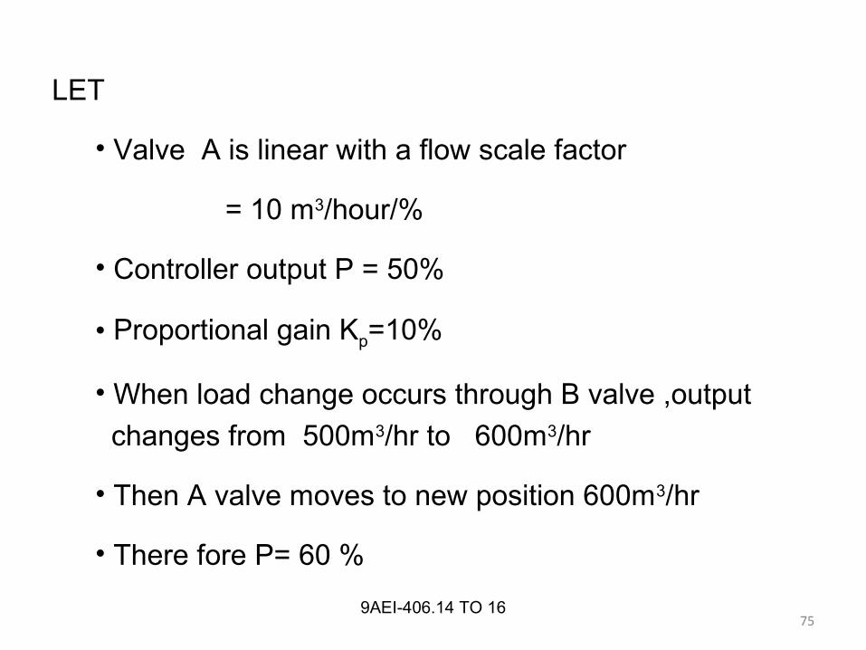
LET

• Valve A is linear with a flow scale factor

= 10 m3/hour/%

• Controller output P = 50%

• Proportional gain Kp=10%

• When load change occurs through B valve ,output

changes from 500m3/hr to 600m3/hr

• Then A valve moves to new position 600m3/hr

• There fore P= 60 %

769AEI-406.14 TO 16

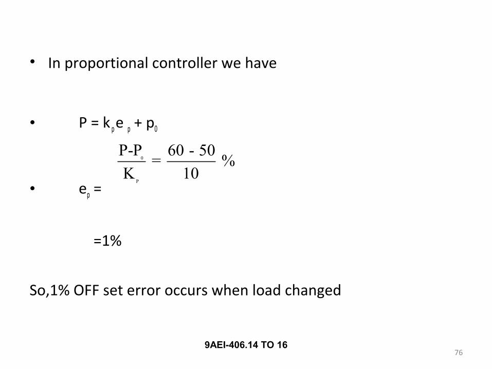
• In proportional controller we have

• P = k p e p + p0

• ep =

=1%

So,1% OFF set error occurs when load changed

0

P

P-P 60 - 50= %

K 10

779AEI-406.14 TO 16

• Offset is eliminated by increase in the proportional gain

which result produces oscillations.

• Fig shows the effect of Kp on the offset.

789AEI-406.14 TO 16

799AEI-406.14 TO 16

9AEI-406.17 & 1880

Integral controller

• Integral action is a mode of action in which the value of the

manipulated variable is changed at rate proporonal to the

derivation.

• Integral controller can also be called as Reset Controller.

9AEI-406.17 & 1881

• If the deviation is double over a previous value , the final

control element is moved twice as faster.

• When the controlled variable is at the set point (zero

deviation), the final control element is stationary.

9AEI-406.17 & 1882

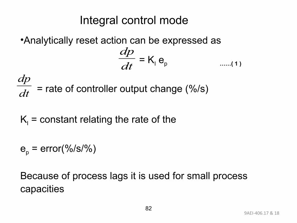
Integral control mode

•Analytically reset action can be expressed as

= KI ep ……( 1 )

= rate of controller output change (%/s)

KI = constant relating the rate of the

ep = error(%/s/%)

Because of process lags it is used for small process capacities

dt

dp

dt

dp

9AEI-406.17 & 1883

• The inverse of K I, called the integral time Ti =1/Ki,

Expressed in seconds or minutes, is used to describe the

integral mode.

• Ti is defined as the time of change of controlled variable

caused by unit change of deviation.

9AEI-406.17 & 1884 84

• For actual controller output equation 1 can be integrated

and is given by

Where p (0) = the controller output at t = 0.

• This equation shows that present controller output p(t)

depends upon the history of error from when obserervation

started at t=0

t

t p

0

p(t) = k e ( t)dt +p(0)∫

9AEI-406.17 & 1885

• If the error doubles ,the rate of controller output change also

doubles.

• The constant ki expressed the scaling between error and

controller output.

• A larger value of ki means that small error produces large

rate of change of p and vice versa.

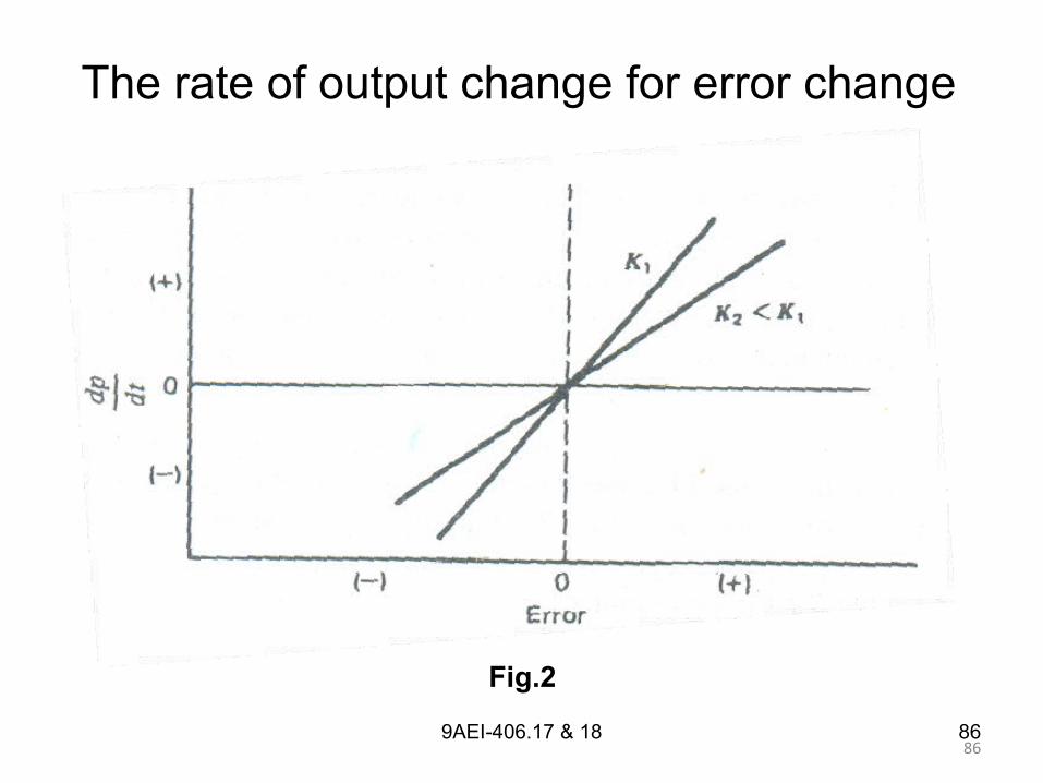
869AEI-406.17 & 18 86

The rate of output change for error change

Fig.2

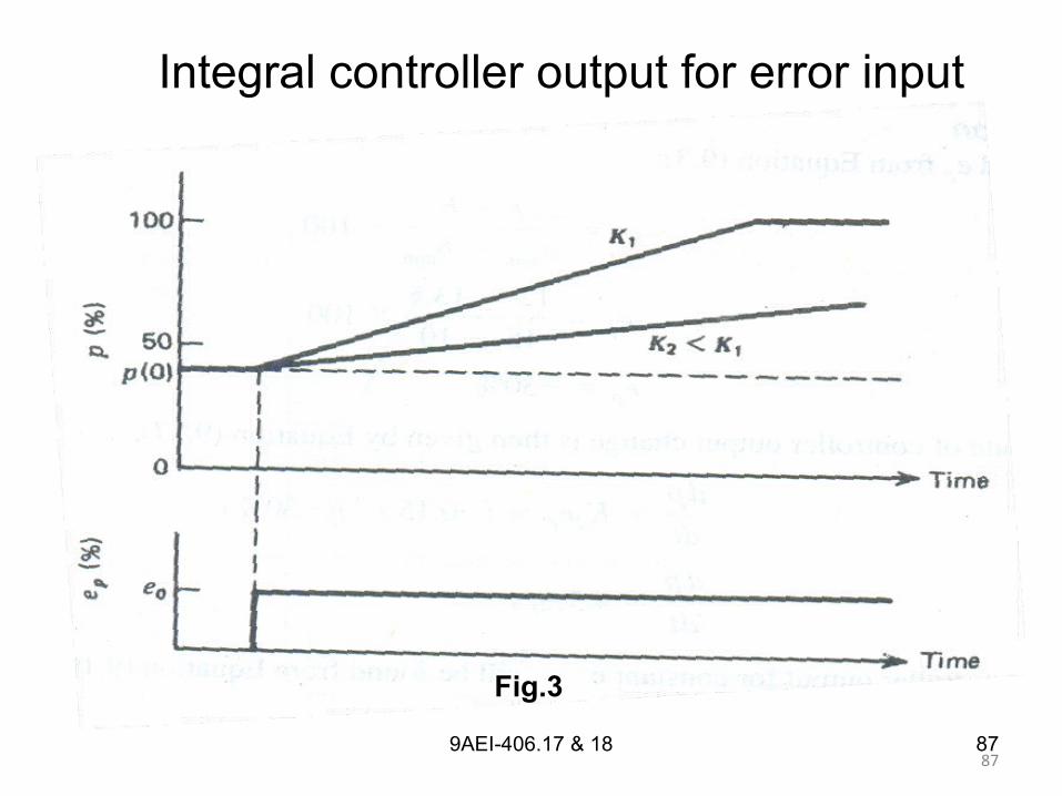
879AEI-406.17 & 18 87

Integral controller output for error input

Fig.3

889AEI-406.17 & 18

• We see that the faster rate provided by Ki cause s much

greater control output at a particular time after the error is

generated.

899AEI-406.17 & 18

Characteristics of integral controller

• If the error is zero, the output stay fixed at a value to what it

was when error went to zero.

• If the error is not zero, the output will begin to increase or

decrease at a rate of ki percent per second for every one

percentage of error.

909AEI-406.17 & 18 90

Integral mode output for error with effect of process and control lag

Fig. 4

919AEI-406.17 & 18

Advantages

• Eliminate the offset.

• Produces sluggish and log oscillation responses.

• If increase gain Kp to produce faster response the system

become more oscillatory and may be led to instability.

91

929AEI-406.17 & 18

Disadvantages

• Slow response

• Process lag is to large cyclic response

939AEI-406.17 & 18

Applications

• The integral control mode is not used alone but can be for

systems with small process lags and correspondingly small

capacities.

949AEI-406.17 & 18

9AEI-406.19 & 2095

Derivative controller

• The derivative mode of controller operation provides that the

controller output depends on the rate of change of error.

9AEI-406.19 & 2096

Other Terms of Derivative controller

• Rate response

• Lead component

• Anticipatory controller

9AEI-406.19 & 2097

Derivative control mode

• Derivative control mode is also known as rate or Anticipatory mode.

• Controller output depends on the rate of change of error

KD = derivative gain constant (%-s/%)

= rate of change of error(%/s)

P = controller output

p

D

deP=K

dt

pde

dt

9AEI-406.19 & 2098

9AEI-406.19 & 2099

9AEI-406.19 & 20100

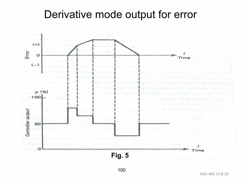
Derivative mode output for error

Fig. 5

9AEI-406.19 & 20101 101

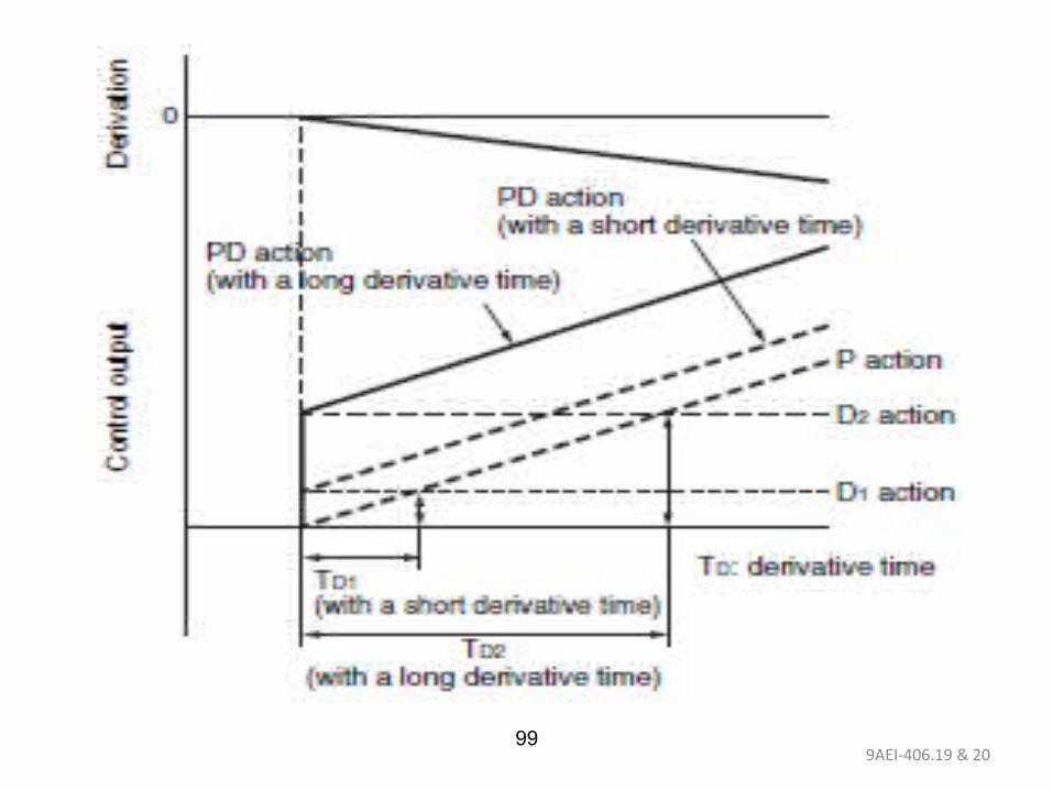
• The characteristics of the derivative control mode

are:

a) If the error is zero, the mode provides no output.

b) If the error is constant in time, the mode provides no

output.

9AEI-406.19 & 20102 102

c) If the error is changing in time, the mode contributes an

output of KD percent for every 1% per second rate of

change of error.

d) For direct action, a positive rate of change of error

produces a positive derivative mode output.

9AEI-406.19 & 20103

Advantages

• The derivative term the controller anticipate what the error

will be in the immediate future and applies control action

which is proportional to the current rate of change of error.

• Fast response (Derivative mode predict process error before

they have evolved and take corrective action in advance of

that occurrence).

9AEI-406.19 & 20104

Disadvantages

• Noisy response with almost zero error it can compute large

derivatives and thus yield large control action, although it is

not needed.

9AEI-406.19 & 20105

Flow controlling

• Chemical reactors

• Petroleum industries

• Power production

Applications

1069AEI-406.21

• This mode is also called as proportional plus reset action

controller.

• Combination of proportional controller and integral

controller is called PI controller.

Proportional + integral control

1079AEI-406.21

• Proportional control mode provides a stabilizing

influence.

• Integral control mode provide corrective action when

deviation in controlled variable from set point.

• Integral control mode has a phase lag of 90º over

proportional control.

• Small process lag permits the use of a large amount of

integral action.

1089AEI-406.21

Analytical expression for controller output in PI

controller

P = Kp ep +Kp KI ∫ep dt +pI(0)

PI(0) = integral term value at t = 0(initial value))

1099AEI-406.21

1109AEI-406.21

Advantages

• Smooth controlling by one to one correspondence of proportional controller.

• Eliminates the offset by integral action.

• It shows a maximum overshoot and settling time similar to the P controller but no steady-state error.

• PI mode can be used in a system with frequent or large load change.

1119AEI-406.21

Disadvantages

• Integration time ,the process must have relatively slow

changes in load to prevent oscillations induced by the integral

overshoot.

• During the start up of a batch process the integral action

causes considerable overshoot error.

1129AEI-406.21

Application

• PI controller can be used in systems with frequent (or)

large load charges.

• Overshoot and cycling often result when PI mode Control is

used in startup of batch process.

112

1139AEI-406.21

Characteristics of PI controller

• When the error is zero the controller out put is fixed at the

value that the integral term had when the error went to zero.

• If the error is not zero, the proportional term contribute a

correction and the integral term begin to increase or decrease

the accumulation value depends on the sign of error and

direct or reverse action

1149AEI-406.21

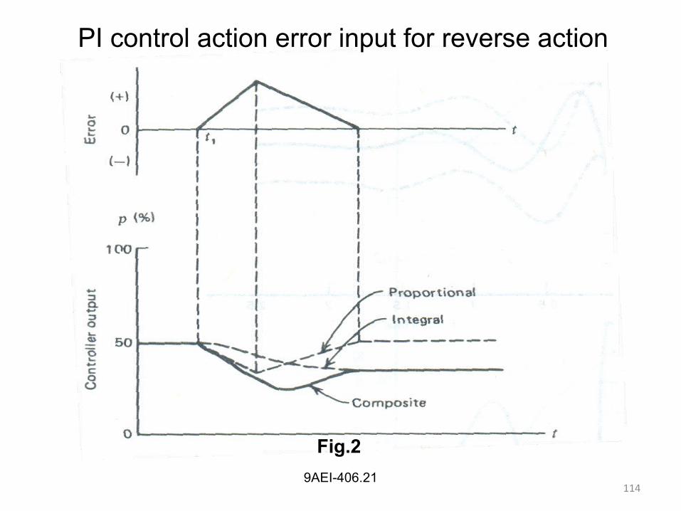
PI control action error input for reverse action

Fig.2

1159AEI-406.22 115

• This mode is also called as proportional plus reset action

controller.

• Combination of proportional controller and Derivative

controller is called PD controller.

Proportional + integral control

1169AEI-406.22

• Derivative action provides the boost necessary to

counter act the time delay associated with such control

systems.

• Derivative control leads proportional control by 90º

Proportional + derivative control

1179AEI-406.22

Analytical expression for PD controller is:

P = Kp ep +Kp KD dep +p0

dt

1189AEI-406.22

1199AEI-406.22

Advantages

• Handled fast process load changes as long as the load

change offset error is acceptable.

• Reduce the magnitude of offset because of narrow

proportional band.

• Properly fits and adjusts to a process and prevent

controlled variable deviation.

• Reduces the time required to stabilize.

1209AEI-406.22

• Used in multi capacity process applications.

• Flow process

• Batching operations like periodic shutdown, emptying

and refilling.

Applications

1219AEI-406.22

Disadvantages

• Does not eliminate offset after a load disturbance.

• It cannot be used where the system lags are less.

1229AEI-406.22 122

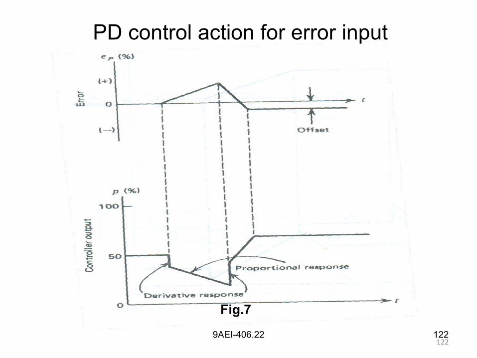
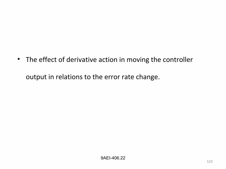
PD control action for error input

Fig.7

1239AEI-406.22

• The effect of derivative action in moving the controller

output in relations to the error rate change.