Embed Size (px)
Citation preview
Solved Problems in Soil Mechanics
Prepared By:
Ahmed S. Al-Agha
February -2016
Based on “Principles of Geotechnical Engineering, 8th Edition”
uniform settlement
(no cracks)
tipping settlement
(often without cracks)
differential settlement
(with cracks)

Being rich is not about how
much you have, but is about how
much you can give
Never let your sense of morals
prevent you from doing what is
right
The more I read, the more I
acquire, the more certain I am
that I know nothing
Chapter (3) & Chapter (6)
Soil Properties
&
Soil Compaction
Page (3)
Soil Properties & Soil Compaction Solved Problems in Soil Mechanics
Ahmed S. Al-Agha
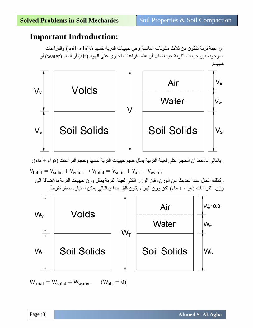
Important Indroduction:
( والفراغات soil solidsعينة تربة تتكون من ثالث مكونات أساسية وهي حبيبات التربة نفسها ) أي
( أو water( أو الماء )airوي على الهواء)الموجودة بين حبيبات التربة حيث تمثل أن هذه الفراغات تحت
كليهما.
وبالتالي نالحظ أن الحجم الكلي لعينة التربية يمثل حجم حبيبات التربة نفسها وحجم الفراغات )هواء + ماء(:
Vtotal = Vsolid + Vvoids → Vtotal = Vsolid + Vair + Vwater
ن الوزن الكلي لعينة التربة يمثل وزن حبيبات التربة باإلضافة الى وكذلك الحال عند الحديث عن الوزن، فإ
وزن الفراغات )هواء + ماء( لكن وزن الهواء يكون قليل جدا وبالتالي يمكن اعتباره صفر تقريباً:
Wtotal = Wsolid + Wwater (Wair = 0)
Page (4)
Soil Properties & Soil Compaction Solved Problems in Soil Mechanics
Ahmed S. Al-Agha
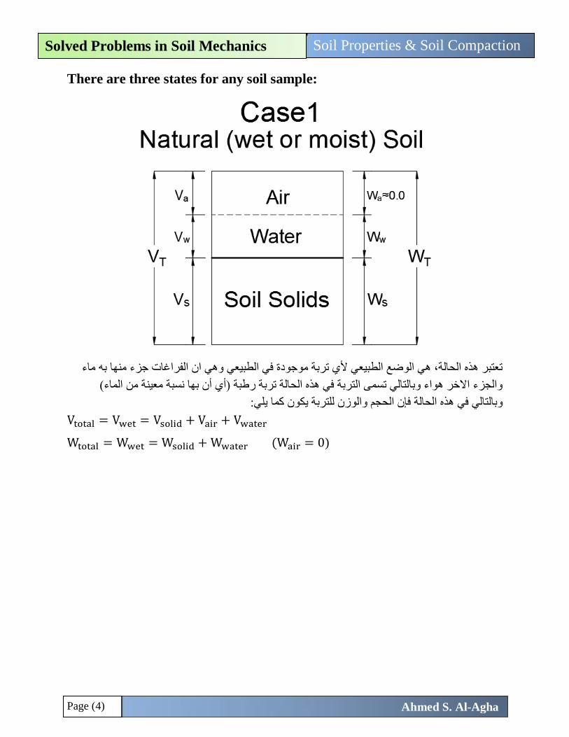
There are three states for any soil sample:
تعتبر هذه الحالة، هي الوضع الطبيعي ألي تربة موجودة في الطبيعي وهي ان الفراغات جزء منها به ماء
والجزء االخر هواء وبالتالي تسمى التربة في هذه الحالة تربة رطبة )أي أن بها نسبة معينة من الماء(
وبالتالي في هذه الحالة فإن الحجم والوزن للتربة يكون كما يلي:
Vtotal = Vwet = Vsolid + Vair + Vwater
Wtotal = Wwet = Wsolid + Wwater (Wair = 0)
Page (5)
Soil Properties & Soil Compaction Solved Problems in Soil Mechanics
Ahmed S. Al-Agha
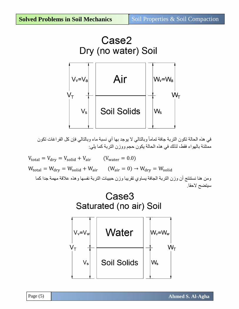
في هذه الحالة تكون التربة جافة تماماً وبالتالي ال يوجد بها أي نسبة ماء وبالتالي فإن كل الفراغات تكون
ون حجم ووزن التربة كما يلي:ممتلئة بالهواء فقط، لذلك في هذه الحالة يك
Vtotal = Vdry = Vsolid + Vair (Vwater = 0.0)
Wtotal = Wdry = Wsolid + Wair (Wair = 0) → Wdry = Wsolid
كما ومن هنا نستنتج أن وزن التربة الجافة يساوي تقريبا وزن حبيبات التربة نفسها وهذه عالقة مهمة جدا
سيتضح الحقا.
Page (6)
Soil Properties & Soil Compaction Solved Problems in Soil Mechanics
Ahmed S. Al-Agha
تكون الفراغات في التربة في هذه الحالة مشبعة كليا بالماء وال تكون أي نسبة للهواء في هذه الحالة، وتسمى
هذه الحالة بحالة التشبع للماء أي أن كل الفراغات متشبعة بالماء وبالتالي يكون حجم الفراغات هو حجم الماء.
بة في هذه الحالة كما يلي:وبالتالي يكون حجم ووزن التر
Vtotal = Vsat = Vsolid + Vwater (Vair = 0.0)
Wtotal = Wsat = Wsolid + Wwater
Density and Unit Weight Calculations
What is the difference between density and unity weight?
Density = ρ =Mass
Volume (kg/m3)
Unit Weight = γ = ρg =Weight
Volume (N/m3)but usually taken in (kN/m3)
( وما ينطبق عليها من قوانين وحسابات unit weightسوف نعتمد في الحسابات والقوانين الكثافة النوعية )
(.densityينطبق تماما على الكثافة )
Unit Weight for water:
It is known that the density of water is 1000 kg/m3, so the unit weight for water
can be calculated as follows:
γwater = ρwater × g = 1000 × 9.81 = 9810 N/m3
γwater = 9810 × 10−3 = 9.81 kN/m3
(.kNحيث سيتم اعتماد هذه القيمة في جميع المسائل التي تتعلق باألوزان ) األوزان تكون بال
Unit Weight for dry (moist) soil (moist unit weight):
γmosit = weight of soil in natural state (case1)
Volume of soil in natural state (case1)=
Wmoist = (Wsolid + Wwater)
Vtotal = (Vsolid + Vwater + Vair)
→ γmosit =Wsolid + Wwater
Vtotal = (Vsolid + Vwater + Vair)
Unit Weight for dry soil (dry unit weight):
هي قيمة مهمة جدا تعبر عن الكثافة النوعية للتربة وهي جافة، حيث كلما زادت هذه القيمة تكون نسبة
ن أكثر تماسكا، ويمكن حسابها كما الفراغات في العينة قليلة وبالتالي تكون حالة التربة جيدة ألن حبيباتها تكو
يلي:
γdry = weight of soil in dry state (case2)
Volume of soil in dry state (case2)=
Wdry = (Wsolid)
Vtotal = (Vsolid + Vair)
→ γdry =Wdry or Wsolid
Vtotal
Page (7)
Soil Properties & Soil Compaction Solved Problems in Soil Mechanics
Ahmed S. Al-Agha
Unit Weight for saturated soil (saturated unit weight):
γsat = weight of soil in saturated state (case3)
Volume of soil in saturated state (case3)=
Wsat = (Wsolid + Wwater)
Vtotal = (Vsolid + Vwater)
→ γsat =Wsolid + Wwater
Vtotal = (Vsolid + Vwater)
Unit Weight for solid particles:
هي قيمة مهمة جدا ألنها تعبر عن كثافة حبيبات التربة نفسها ويساوي وزن حبيبات التربة نفسها مقسوما على
حجم حبيبات التربة نفسها.
γsolid =Wsolid = (Wdry)
Vsolid
Specific Gravity for soil solids:
بين كثافة أي مادة وكثافة الماء، وبالتالي تعتبر هذه القيمة خاصية مهمة بشكل عام فإن هذه القيمة تمثل النسبة
جدا ألي مادة، ألنها تعبر عن مدى قرب أو بعد كثافة المادة من كثافة الماء، هنا نحن نهتم بحساب هذه القيمة
التربة حيث ( حيث أن هذه القيمة تعتبر خاصية مهمة جدا ألي نوع من soil solidsلحبيبات التربة نفسها )
تعبر عن مدى قوى التربة وتماسكها أو ضعفها.
Gs = γsolid
γwater
تقريبا، وهي ليس لها وحدة ألنها نسبة بين 3إلى 2.2في العادة تتراوح هذه القيمة لمختلف أنواع التربة من
قيمتين لهما نفس الوحدة.
Void Ratio:
مدى قوة وتماسك التربة أو مدى ضعفها ألنها تمثل النسبة بين حجم الفراغات هذه القيمة مهمة جدا في تحديد
الكلي )هواء + ماء( الموجود في العينة بالنسبة إلى حجم حبيبات التربة نفسها، حيث كلما كانت هذه القيمة
رة تكون صغيرة تكون الفراغات في التربة قليلة وتكون التربة متماسكة وقوية، لكن اذا كانت القيمة كبي
الفراغات نسبتها كبيرة بالنسبة لحبيبات التربة نفسها وبالتالي تكون التربة ضعيفة وغير متماسكة.
e =Vvoids
Vsolid=
VT − Vs
Vs
يكون حجم الفراغات اقل من حجم حبيبات التربة نفسها وبالتالي تكون التربة 1اذا كانت هذه القيمة أقل من
يكون 1، ولكن اذا كانت هذه القيمة أكبر من 1سكة وتزادا درجة التماسك كلما قلت هذه النسبة عن قوية ومتما
حجم الفراغات أكبر من حجم حبيبات التربة نفسها وتكون التربة في هذه الحالة ضعيفة ومفككة، وكلما زادت
كلما ازدادت حالة التربة سوءاً. 1هذه القيمة عن
تصل للصفر، ألنه دائما يكون نسبة فراغات ولو كانت صغيرة، لكن كلما اقتربت من هذه القيمة ال يمكن أن
الصفر تكون التربة قوية جدا وأفضل ما يمكن.
Page (8)
Soil Properties & Soil Compaction Solved Problems in Soil Mechanics
Ahmed S. Al-Agha
There are very important relationship for calculating 𝛄𝐝𝐫𝐲:
γdry =Gs × γw
1 + e
This is very important relationship and you should recognize it.
This equation is derived from the following relationships:
γdry =Wdry or Wsolid
Vtotal , γsolid =
Wsolid = (Wdry)
Vsolid , Gs =
γsolid
γwater
γdry =Wdry
Vtotal→ Wdry = γdry × Vtotal → Eq. (1)
Also, γsolid =Wsolid=(Wdry)
Vsolid→ Wdry = γsolid × Vsolid → Eq. (2)
By equating Eq.(1) and Eq.(2):
γdry × Vtotal = γsolid × Vsolid → γdry =γsolid × Vsolid
Vtotal→ Eq. (3)
And we know that, Gs = γsolid
γwater→ γsolid = Gs × γwater (Substitute in Eq. (3))
→ γdry =Gs × γw × Vs
VT → Eq. (4)
e =VT − Vs
Vs , but we want the value of
Vs
VT and we can write the equation as:
→ e =VT
Vs− 1 →
VT
Vs= e + 1 →
Vs
VT=
1
e + 1 (Substitute in Eq. (4)
→ γdry =Gs × γw
1 + e (proofed)
Another frequently used relationship which is very important:
S. e = Gs. w
S = Degree of saturation
ء من الفراغات وبالتالي تعبر هذه القيمة عن نسبة الماء الموجودة في الفراغات، أي النسبة التي تمثلها الما
تمثل هذه القيمة النسبة بين حجم الماء وحجم الفراغات:
S =Vwater
Vvoids
وبالتالي عندما تكون التربة مشبعة بالماء فإن الفراغات كلها تكون مشبعة بالماء وبالتالي حجم الفراغات
قيمة يمكن ان تصلها.وهي اقصى 1يساوي حجم الماء وبالتالي تكون درجة التشبع تساوي
At Saturation, → Vvoids = Vwater → S = 1
Page (9)
Soil Properties & Soil Compaction Solved Problems in Soil Mechanics
Ahmed S. Al-Agha
w = water content in the soil specimen →→
w =Weight of water
Weight of solid=
Ww
Ws=
Wwet − Wdry
Wdry × 100%
How you can proof this relationship (S. e = Gs. w)???
S =Vw
Vv → Eq. (1)
Vwater =Ww
γw → Eq. (2)
w =Ww
Ws→ Ww = w × Ws → Eq. (3)
Ws =? ? ?
γs =Ws
Vs→ Ws = γs × Vs, but we know that Gs =
γs
γw→ γs = Gs × γw
→ Ws = Gs × γw × Vs (substitute in Eq. (3)) →→
Ww = w × Gs × γw × Vs (substitute in Eq. (2)) →→
Vw =w × Gs × γw × Vs
γw= w × Gs × Vs (substitute in Eq. (1)) →→
S =w × Gs × Vs
Vv→ S ×
Vv
Vs= w × Gs (but we know that
Vv
Vs= e) →
S × e = w × Gs (proofed)
Calculation of moist and saturated unit weight:
γmoist = γdry × (1 + %w)
But we know that , γdry =Gs × γw
1 + e →
→ γmoist =Gs × γw × (1 + w)
1 + e
γsat = γdry × (1 + wsat)
→ γsat =Gs × γw × (1 + wsat)
1 + e
But we know that, at saturation S = 1:
S. e = Gs. w → at saturation → Ssat. e = Gs. wsat
→ wsat =Ssat.e
Gs (but Ssat = 1) → wsat =
e
Gs(substitute in equation ofγsat)
Page (10)
Soil Properties & Soil Compaction Solved Problems in Soil Mechanics
Ahmed S. Al-Agha
→ γsat =Gs × γw × (1 +
eGs
)
1 + e
Calculation of maximum dry unit weight:
We know that the value of dry unit weight can be calculated from the following
equation:
γdry =Gs × γw
1 + e
For any type soil, the value of Gs is constant, and also the value of γw is always
constant (at natural state), so the only variable in the above equation is the void
ratio e, and as the value of e decreased the value of γdry increased (as shown in the
equation), so if we obtain to the minimum value of e, we get the maximum value
of γdry.
How to calculate the minimum value of e?:
S. e = Gs. w → e =Gs. w
S→ To get the minimum value for e, the value of S
should maximum value, and we know the maximum value of S is 1, so:
emin =Gs × w
S = 1= Gs × w (Substitute in γdry equation):
→ γdry,max =Gs × γw
1 + emin→ γdry,max =
Gs × γw
1 + Gs × w
This value is also called Zero Air Voids (ZAV) dry unit weight.
وذلك ألنه في هذه الحالة تكون كل الفراغات مشبعة كليا بالماء وال تكون أي نسبة هواء وبالتالي يمكن
تسميتها بهذا اإلسم أيضاً.
γdry,max = γZ.A.V =Gs × γw
1 + Gs × w
Another important properties of soil:
Porosity (n):
الفراغات إلى الحجم سبة الفراغات الموجودة في العينة الكلية، أي أنها تمثل النسبة بين حجم وهي تمثل ن
الكلي للعينة، وهي خاصية مهمة جدا خصوصا في حاالت دراسات تسرب مياه األمطار إلى المياه الجوفية:
n =Vvoids
Vtotal=
VT − Vs
VT (and we know that e =
VT − Vs
Vs) → n =
e
1 + e
Page (11)
Soil Properties & Soil Compaction Solved Problems in Soil Mechanics
Ahmed S. Al-Agha
Air Content (A):
لى الحجم الكلي عتمثل هذه القيمة نسبة الهواء الموجودة في عينة التربة، وبالتالي تمثل النسبة بين حجم الهواء
ك حبيبات التربة:كللعينة وهي قيمة مهمة لتحديد نسبة فراغات الهواء في التربة وبالتالي مدى تماسك أو تفك
Air content (A) =Vair
Vtotal
Relative Density (Dr):
أو مدى تفككها وانحاللها ويتم حسابها كما هي قيمة مهمة جدا وهي تعبر عن مدى تماسك وكثافة عينة التربة
يلي:
Dr =emax − e
emax − emin OR Dr =
1γdmin
−1
γd
1γdmin
−1
γdmax
emax = max. value for void ratio and can be determined from lab for any soil.
emin = min. value for void ratio and can be determined from the properties
of soil → emin = Gs × w (as clarified above).
e = the current value for the soil.
الحالية هي اقصى void ratioة لهذ الخاصية قد تكون صفر وهي عندما تكون قيمة ال نالحظ أن أقل قيم
:قيمة يمكن أن تصلها وبالتالي يكون البسط في المعادلة صفر، وتكون التربة في هذه الحالة في أسوأ األحوال
((Loosest Condition وذلك عندما تكون قيمة ال 1، وأقصى قيمة لهذه الخاصية تكونvoid ratio
الحالية هي أقل قيمة يمكن أن تصلها التربة وبالتالي فإن البسط يساوي المقام في هذه الحالة وتكون القيمة
.1مساوية
Relative Compaction(R. C):
هي أيضا قيمة مهمة جدا في كل المشاريع الهندسية ألنها تعبر عن درجة الدمك لعينة التربة، حيث تمثل
الحقيقية للعينة في الموقع إلى أقصى كثافة يمكن الحصول عليها مخبريا لنفس عينة التربة النسبة بين الكثافة
القيمة تعتبر أساس في كل المشاريع الهندسية، حيث يجب حسابها للتربة الموجودة في الموقع، وبالتالي هذه
حيث يمكن 100ال % ويمكن ان تتجاوز 95ويجب أن تحقق التربة قيمة معينة حتى تكون التربة مقبولة %
، وهذا يعني ان كثافة العينة في الموقع قوية جدا ) حيث تزداد هذه القيمة بزيادة الدمك 105ان تصل الى %
أو أكثر وذلك حسب ما تحدده 85في الموقع(، وأحيانا تكون القيمة المقبولة )في بعض المشاريع( %
مواصفات المشروع، ويمكن حساب هذه القيمة كما يلي:
Relative Compaction(R. C) =γdry,max,field
γdry,max,proctor× 100%
Page (12)
Soil Properties & Soil Compaction Solved Problems in Soil Mechanics
Ahmed S. Al-Agha
Important values and conversions:
γwater = 9.81KN/m3 = 62.4Ib/ft3 , 1ton = 2000Ib , 1yd3 =27ft
3
1m = 0.3048 ft
1ft = 12 inch
1inch = 2.54 cm
1Ib = 4.45 N
γw = 9810N
m3×
Ib
4.45N×
(0.3048)3m3
ft3= 62.4 Ib/ft3
g = 9.81m
S2×
ft
0.3048m= 32.2ft/S2
Volume of cone (Vcone) =π
3R2 × h )ثلث حجم االسطوانة(
1m3 = 106 cm3 .
1m3 = 109 mm3 .
Important Note:
Vsolid must be constant if we want to use the borrow pit soil in a construction site
or on earth dam or anywhere else.
Page (13)
Soil Properties & Soil Compaction Solved Problems in Soil Mechanics
Ahmed S. Al-Agha
1. (Mid 2015): A construction site requires 100m
3 of soil compacted at the maximum dry density
estimated from laboratory standard compaction tests. Laboratory tests indicate the
optimum moisture content is 12% and the degree of saturation at optimum is 85%.
If the specific gravity is 2.7.
a) Calculate the weight of dry soil required at the construction site.
b) Calculate the total weight of soil that needs to be transported to the site if it is
extracted from a borrow pit with a moisture content of 5%.
Solution
Givens:
VT = 100 m3 , %w = 12% , S = 85% , Gs = 2.7
a) Wdry = Wsolid =? ? ?
Calculate the void ratio as following:
S. e = Gs. w → 0.85 × e = 2.7 × 0.12 → e = 0.381
Calculate the value of dry unit weight:
γdry =Gs × γw
1 + e=
2.7 × 9.81
1 + 0.381= 19.18 kN/m3
γdry = 19.18 =Wdry
Vtotal=
Wdry
100→ Wdry = 1918 kN ✓.
b) WTotal from bprrow pit =? ? if %w = 5%
، ألن الحبيبات الصلبة ال يتغير وزنها تكون ثابتة وال تتغير Wsعينة تربة دائما وأبدا قيمة يأل هامة:مالحظة
وال يتغير حجمها، ولكن الذي يتغير هو حجم الفراغات ونسبة الفراغات.
w =Wwet − Wdry
Wdry → 0.05 =
Wwet − 1918
1918→ 2013.9 kN✓.
ن الماء( حيث أن وزن الهواء وزن العينة ارطب يمثل الوزن الكلي للعينة )وزن الحبيبات الصلبة + وز
يتم اهماله ألنه صغير جدا.
Page (14)
Soil Properties & Soil Compaction Solved Problems in Soil Mechanics
Ahmed S. Al-Agha
2. (Mid 2014):
a) Show the saturated moisture content is: Wsat = γw [1
γd−
1
γs]
𝐇𝐢𝐧𝐭: γs = solid unit weight
Solution
S. e = Gs. w , at saturation → S = 1 → wsat =e
Gs→→ Eq. (1)
γd =Gs × γw
1 + e→ e =
Gs × γw
γd− 1, substitute in Eq. (1) →→
wsat =
Gs × γw
γd− 1
Gs=
γw
γd−
1
Gs but Gs =
γs
γw→
1
Gs=
γw
γs→→
wsat =γw
γd−
γw
γs= γw [
1
γd−
1
γs]✓ .
b) A geotechnical laboratory reported these results of five samples taken from a
single boring. Determine which are not correctly reported, if any, show your work. 𝐇𝐢𝐧𝐭: take γw = 9.81kN/m3
Sample #1: w = 30%, γd = 14.9 kN/m3, γs = 27 kN/m3 , clay
Sample #2: w = 20%, γd = 18 kN/m3, γs = 27 kN/m3 , silt
Sample #3: w = 10%, γd = 16 kN/m3, γs = 26 kN/m3 , sand
Sample #4: w = 22%, γd = 17.3 kN/m3, γs = 28 kN/m3 , silt
Sample #5: w = 22%, γd = 18 kN/m3, γs = 27 kN/m3 , silt
Solution
For any type of soil, the mositure content (w) must not exceeds the saturated
moisture content, so for each soil we calculate the saturated moisture content from
the derived equation in part (a) and compare it with the given water content.
Sample #1: (Given water content= 30%)
wsat = 9.81 [1
14.9−
1
27] = 29.5% < 30% → not correctly reported✓.
Sample #2: (Given water content= 20%)
Page (15)
Soil Properties & Soil Compaction Solved Problems in Soil Mechanics
Ahmed S. Al-Agha
wsat = 9.81 [1
18−
1
27] = 18.16% < 20% → not correctly reported✓.
Sample #3: (Given water content= 10%)
wsat = 9.81 [1
16−
1
26] = 23.58% > 10% → correctly reported✓.
Sample #4: (Given water content= 22%)
wsat = 9.81 [1
17.3−
1
28] = 21.67% < 22% → not correctly reported✓.
Sample #5: (Given water content= 22%)
wsat = 9.81 [1
18−
1
27] = 18.16% < 22% → not correctly reported✓.
Page (16)
Soil Properties & Soil Compaction Solved Problems in Soil Mechanics
Ahmed S. Al-Agha
3. (Mid 2013): If a soil sample has a dry unit weight of 19.5 KN/m
3, moisture content of 8%
and a specific gravity of solids particles is 2.67. Calculate the following:
a) The void ratio.
b) Moisture and saturated unit weight.
c) The mass of water to be added to cubic meter of soil to reach 80% saturation.
d) The volume of solids particles when the mass of water is 25 grams for saturation.
Solution
Givens:
γdry = 19.5KN/m3 , %w = 8% , Gs=2.67
a)
γdry =Gs × γw
1 + e→ 19.5 =
2.67 × 9.81
1 + e→ e = 0.343 ✓
b)
∗ γmoist = γdry(1 + %w) = 19.5 × (1 + 0.08) = 21.06 KN/m3 ✓
∗ γsat = γdry(1 + %wsat) → %wsat means %w @ S = 100%
S.e = Gs.w→ %wsat =S.e
Gs=
1×0.343
2.67× 100% = 12.85%
So, . . γsat = 19.5(1 + 0.1285) = 22 KN/m3 ✓
c)
γmoist = 21.06 KN/m3 وهي القيمة األصلية الموجودة في المسألة →
Now we want to find γmoist @ 80% Saturation so, firstly we calculate %w @80%
saturation:
%w80% =S. e
Gs=
0.8 × 0.343
2.67× 100% = 10.27%
γmoist,80% = 19.5(1 + 0.1027) = 21.5 KN/m3
Weight of water to be added = 21.5-21.06 = 0.44 KN/m3✓
Mass of water to be added = 0.44×1000
9.81= 44.85 Kg/m3✓
Page (17)
Soil Properties & Soil Compaction Solved Problems in Soil Mechanics
Ahmed S. Al-Agha
Another solution:
VT = 1m3 → ي الكمية التي يجب إضافة الماء إليها والموجودة في نص المطلوب وه
The water content before adding water (%w1) = 8%
The water content after adding water (%w2) = 10.27% @80%saturation
w =Weight of water
Weight of solid=
Ww
Ws
تكون ثابتة وال تتغير Wsينة تربة دائما وأبدا قيمة ع ي: ألهامةمالحظة
γdry =Ws
VT→ Ws = 19.5 × 1 = 19.5KN
Ww = Ws × w → Ww,1 = Ws × w1 , and Ww,2 = Ws × w2
Then, Ww,1 = 19.5 × 0.08 = 1.56 KN
Ww,2 = 19.5 × 0.1027 = 2 KN
Weight of water to be added = 2-1.56= 0.44 KN ✓
Mass of water to be added = 0.44×1000
9.81= 44.85 Kg ✓
d)
Mw = 25grams for saturation → S = 100% → %wsat = 12.85%
Ww = (25 × 10−3)Kg ×9.81
1000= 24.525 × 10⁻⁵KN
Ws =Ww
w=
24.525 × 10⁻⁵
0.1285= 190.85 × 10⁻⁵ KN
Now, Gs = γsolid
γwater→ γsolid = 2.67 × 9.81 = 26.2KN/m3
γsolid = Ws
Vs→ Vs =
Ws
γsolid=
190.85×10⁻⁵
26.2= 7.284 × 10⁻⁵ m3 =72.84 cm
3 ✓
Page (18)
Soil Properties & Soil Compaction Solved Problems in Soil Mechanics
Ahmed S. Al-Agha
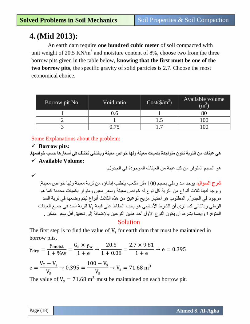
4. (Mid 2013): An earth dam require one hundred cubic meter of soil compacted with
unit weight of 20.5 KN/m3 and moisture content of 8%, choose two from the three
borrow pits given in the table below, knowing that the first must be one of the
two borrow pits, the specific gravity of solid particles is 2.7. Choose the most
economical choice.
Some Explanations about the problem:
Borrow pits:
معينة ولها خواص معينة وبالتالي تختلف في أسعارها حسب خواصها. هي عينات من التربة تكون متواجدة بكميات
Available Volume:
هو الحجم المتوفر من كل عينة من العينات الموجودة في الجدول.
ص معينة, يتطلب إنشاؤه من تربة معينة ولها خوا متر مكعب 100بحجم يوجد سد رملي شرح السؤال:
ويوجد لدينا ثالث أنواع من التربة كل نوع له خواص معينة وسعر معين ومتوفر بكميات محددة كما هو
من هذه الثالث أنواع ليتم وضعها في تربة السد نوعينموجود في الجدول, المطلوب هو اختيار مزيج
لتربة السد في جميع العينات Vsبالتالي كما نرى أن الشرط األساسي هو يجب الحفاظ على قيمة و الرملي
تحقيق أقل سعر ممكن . باإلضافة إلىهذين النوعين أحدالمتوفرة وأيضا بشرط أن يكون النوع األول
Solution
The first step is to find the value of Vs for earth dam that must be maintained in
borrow pits.
γdry =γmoist
1 + %w=
Gs × γw
1 + e→
20.5
1 + 0.08=
2.7 × 9.81
1 + e→ e = 0.395
e =VT − Vs
Vs→ 0.395 =
100 − Vs
Vs→ Vs = 71.68 m3
The value of Vs = 71.68 m3 must be maintained on each borrow pit.
Borrow pit No. Void ratio Cost($/m3)
Available volume
(m3)
1 0.6 1 80
2 1 1.5 100
3 0.75 1.7 100
Page (19)
Soil Properties & Soil Compaction Solved Problems in Soil Mechanics
Ahmed S. Al-Agha
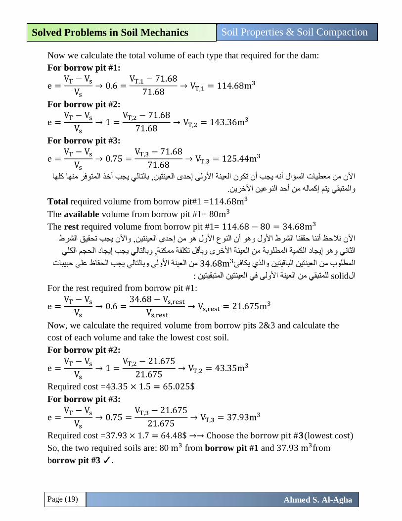
Now we calculate the total volume of each type that required for the dam:
For borrow pit #1:
e =VT − Vs
Vs→ 0.6 =
VT,1 − 71.68
71.68→ VT,1 = 114.68m3
For borrow pit #2:
e =VT − Vs
Vs→ 1 =
VT,2 − 71.68
71.68→ VT,2 = 143.36m3
For borrow pit #3:
e =VT − Vs
Vs→ 0.75 =
VT,3 − 71.68
71.68→ VT,3 = 125.44m3
أخذ المتوفر منها كلها باآلن من معطيات السؤال أنه يجب أن تكون العينة األولى إحدى العينتين, بالتالي يج
والمتبقي يتم إكماله من أحد النوعين اآلخرين.
Total required volume from borrow pit#1 =114.68m3
The available volume from borrow pit #1= 80m3
The rest required volume from borrow pit #1= 114.68 − 80 = 34.68m3
حدى العينتين, واآلن يجب تحقيق الشرط إاآلن نالحظ أننا حققنا الشرط األول وهو أن النوع األول هو من
م الكلي من العينة األخرى وبأقل تكلفة ممكنة, وبالتالي يجب إيجاد الحجالمطلوبة هو إيجاد الكمية والثاني
يجب الحفاظ على حبيبات وبالتاليمن العينة األولى 34.68m3المطلوب من العينتين الباقيتين والذي يكافئ
للمتبقي من العينة األولى في العينتين المتبقيتين : solidال
For the rest required from borrow pit #1:
e =VT − Vs
Vs→ 0.6 =
34.68 − Vs,rest
Vs,rest→ Vs,rest = 21.675m3
Now, we calculate the required volume from borrow pits 2&3 and calculate the
cost of each volume and take the lowest cost soil.
For borrow pit #2:
e =VT − Vs
Vs→ 1 =
VT,2 − 21.675
21.675→ VT,2 = 43.35m3
Required cost =43.35 × 1.5 = 65.025$
For borrow pit #3:
e =VT − Vs
Vs→ 0.75 =
VT,3 − 21.675
21.675→ VT,3 = 37.93m3
Required cost =37.93 × 1.7 = 64.48$ →→ Choose the borrow pit #𝟑(lowest cost)
So, the two required soils are: 80 m3 from borrow pit #1 and 37.93 m3from
borrow pit #3 ✓.
Page (20)
Soil Properties & Soil Compaction Solved Problems in Soil Mechanics
Ahmed S. Al-Agha
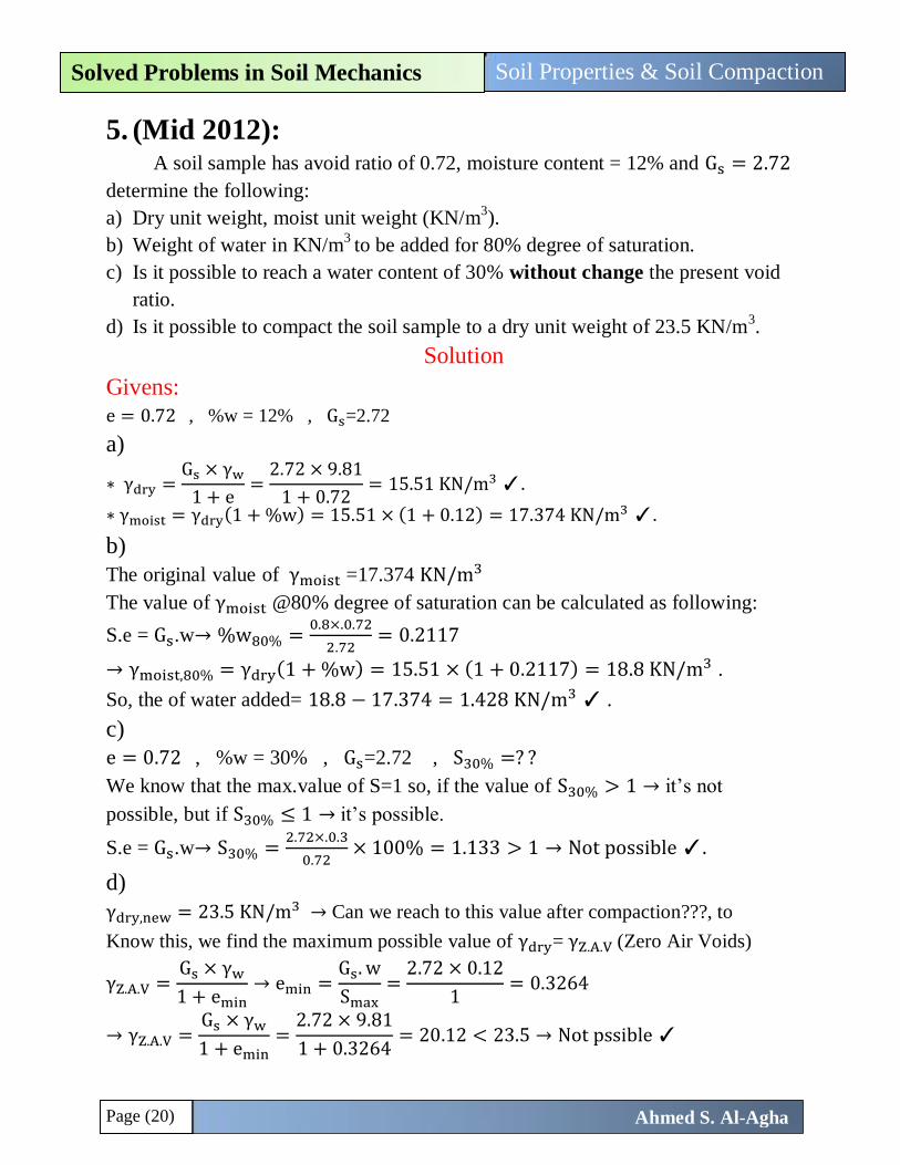
5. (Mid 2012): A soil sample has avoid ratio of 0.72, moisture content = 12% and Gs = 2.72
determine the following:
a) Dry unit weight, moist unit weight (KN/m3).
b) Weight of water in KN/m3
to be added for 80% degree of saturation.
c) Is it possible to reach a water content of 30% without change the present void
ratio.
d) Is it possible to compact the soil sample to a dry unit weight of 23.5 KN/m3.
Solution
Givens:
e = 0.72 , %w = 12% , Gs=2.72
a)
∗ γdry =Gs × γw
1 + e=
2.72 × 9.81
1 + 0.72= 15.51 KN/m3 ✓.
∗ γmoist = γdry(1 + %w) = 15.51 × (1 + 0.12) = 17.374 KN/m3 ✓.
b)
The original value of γmoist =17.374 KN/m3
The value of γmoist @80% degree of saturation can be calculated as following:
S.e = Gs.w→ %w80% =0.8×.0.72
2.72= 0.2117
→ γmoist,80% = γdry(1 + %w) = 15.51 × (1 + 0.2117) = 18.8 KN/m3 .
So, the of water added= 18.8 − 17.374 = 1.428 KN/m3 ✓ .
c)
e = 0.72 , %w = 30% , Gs=2.72 , S30% =? ?
We know that the max.value of S=1 so, if the value of S30% > 1 → it’s not
possible, but if S30% ≤ 1 → it’s possible.
S.e = Gs.w→ S30% =2.72×.0.3
0.72× 100% = 1.133 > 1 → Not possible ✓.
d)
γdry,new = 23.5 KN/m3 → Can we reach to this value after compaction???, to
Know this, we find the maximum possible value of γdry= γZ.A.V (Zero Air Voids)
γZ.A.V =Gs × γw
1 + emin→ emin =
Gs. w
Smax=
2.72 × 0.12
1= 0.3264
→ γZ.A.V =Gs × γw
1 + emin
=2.72 × 9.81
1 + 0.3264= 20.12 < 23.5 → Not pssible ✓
Page (21)
Soil Properties & Soil Compaction Solved Problems in Soil Mechanics
Ahmed S. Al-Agha
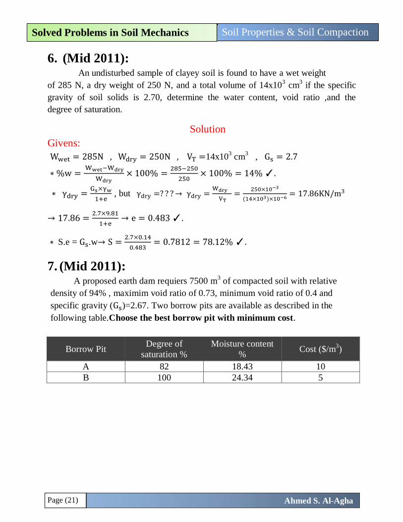
6. (Mid 2011): An undisturbed sample of clayey soil is found to have a wet weight
of 285 N, a dry weight of 250 N, and a total volume of 14x103 cm
3 if the specific
gravity of soil solids is 2.70, determine the water content, void ratio ,and the
degree of saturation.
Solution
Givens:
Wwet = 285N , Wdry = 250N , VT =14x103 cm
3 , Gs = 2.7
∗ %w = Wwet−Wdry
Wdry× 100% =
285−250
250× 100% = 14% ✓.
∗ γdry =Gs×γw
1+e , but γdry =? ? ? → γdry =
Wdry
VT=
250×10−3
(14×103)×10−6= 17.86KN/m3
→ 17.86 =2.7×9.81
1+e→ e = 0.483 ✓.
∗ S.e = Gs.w→ S =2.7×0.14
0.483= 0.7812 = 78.12% ✓.
7. (Mid 2011):
A proposed earth dam requiers 7500 m3 of compacted soil with relative
density of 94% , maximim void ratio of 0.73, minimum void ratio of 0.4 and
specific gravity (Gs)=2.67. Two borrow pits are available as described in the
following table.Choose the best borrow pit with minimum cost.
Borrow Pit Degree of
saturation %
Moisture content
% Cost ($/m
3)
A 82 18.43 10
B 100 24.34 5
Page (22)
Soil Properties & Soil Compaction Solved Problems in Soil Mechanics
Ahmed S. Al-Agha
Solution
Givens:
Dr = 94% , emax = 0.73 , emin = 0.4 , Gs = 2.67
)العينات الموجودة في الجدول(حضارها للسد إللسد من أي عينة تربة نريد Vs فكرة الحل أنه يجب الحفاظ على قيمة
So, firstly we calculate the value of Vs that required for earth dam as following:
e =Vv
Vs=
VT−Vs
Vs , but e =? ? ? → Dr =
emax−e
emax−emin→ 0.94 =
0.73−e
0.73−0.4→ e = 0.42
→ 0.42 =7500−Vs
Vs→ Vs = 5281.7m3 that must be maintained.
Vs اآلن, حتى نجد سعر كل عينة يجب تحديد الحجم الكلي لكل عينة والذي يحقق قيمة = 5281.7
For sample “ A “ :
S =82% , %w =18.43%
e =VT − Vs
Vs, but e =? ? ? → e =
Gs × w
S=
2.67 × 0.1843
0.82= 0.6
→ 0.6 =VT − 5281.7
5281.7→ VT = 8450.72 m3.
So, the total cost for sample “ A “ =8450.72 m3 × 10$
m3= 84,507$ .
For sample “ B “ :
S =100% , %w =24.34%
e =VT − Vs
Vs, but e =? ? ? → e =
Gs × w
S=
2.67 × 0.2434
1= 0.65
→ 0.65 =VT − 5281.7
5281.7→ VT = 8714.8 m3.
So, the total cost for sample “ B “ =8714.8 m3 × 5$
m3= 43,574$ .
So, we choose the sample “ B “ beacause it has the lowest cost ✓.
Page (23)
Soil Properties & Soil Compaction Solved Problems in Soil Mechanics
Ahmed S. Al-Agha
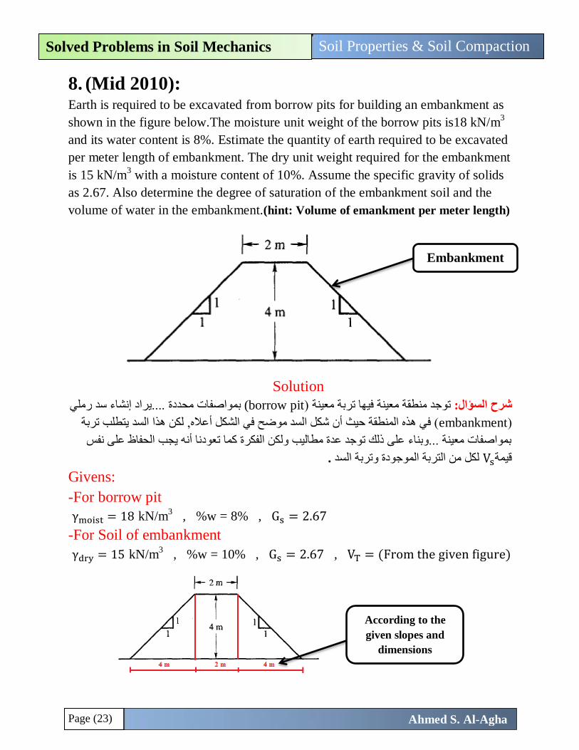
8. (Mid 2010):
Earth is required to be excavated from borrow pits for building an embankment as
shown in the figure below.The moisture unit weight of the borrow pits is18 kN/m3
and its water content is 8%. Estimate the quantity of earth required to be excavated
per meter length of embankment. The dry unit weight required for the embankment
is 15 kN/m3 with a moisture content of 10%. Assume the specific gravity of solids
as 2.67. Also determine the degree of saturation of the embankment soil and the
volume of water in the embankment.(hint: Volume of emankment per meter length)
Solution
....يراد إنشاء سد رملي محددةبمواصفات borrow pit)ها تربة معينة )فيتوجد منطقة معينة :شرح السؤال
(embankmentفي هذه المنطقة حيث أن شكل السد موضح في الشكل أعاله ), بة لكن هذا السد يتطلب تر
بمواصفات معينة ...وبناء على ذلك توجد عدة مطاليب ولكن الفكرة كما تعودنا أنه يجب الحفاظ على نفس
. لكل من التربة الموجودة وتربة السد Vsقيمة
Givens:
-For borrow pit
γmoist = 18 kN/m3 , %w = 8% , Gs = 2.67
-For Soil of embankment
γdry = 15 kN/m3 , %w = 10% , Gs = 2.67 , VT = (From the given figure)
Embankment
According to the
given slopes and
dimensions
Page (24)
Soil Properties & Soil Compaction Solved Problems in Soil Mechanics
Ahmed S. Al-Agha
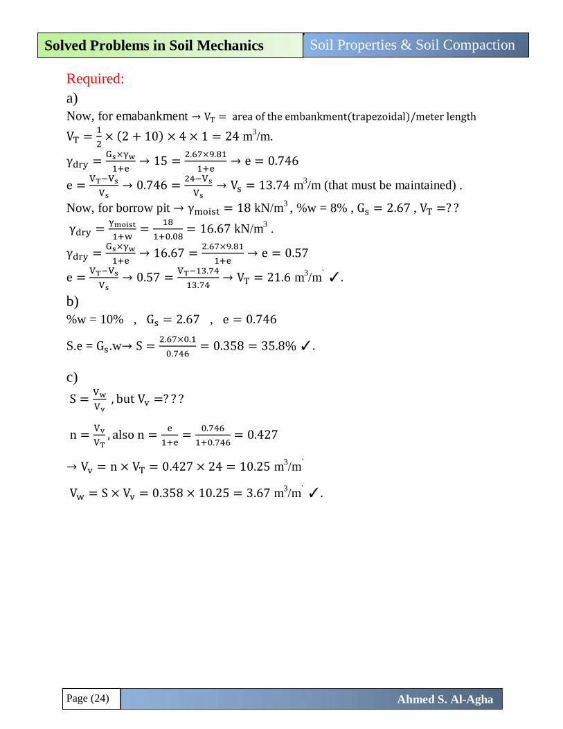
Required:
a)
Now, for emabankment → VT = area of the embankment(trapezoidal)/meter length
VT =1
2× (2 + 10) × 4 × 1 = 24 m
3/m.
γdry =Gs×γw
1+e→ 15 =
2.67×9.81
1+e→ e = 0.746
e =VT−Vs
Vs→ 0.746 =
24−Vs
Vs→ Vs = 13.74 m
3/m (that must be maintained) .
Now, for borrow pit → γmoist = 18 kN/m3
, %w = 8% , Gs = 2.67 , VT =? ?
γdry =γmoist
1+w=
18
1+0.08= 16.67 kN/m
3 .
γdry =Gs×γw
1+e→ 16.67 =
2.67×9.81
1+e→ e = 0.57
e =VT−Vs
Vs→ 0.57 =
VT−13.74
13.74→ VT = 21.6 m
3/m
` ✓.
b)
%w = 10% , Gs = 2.67 , e = 0.746
S.e = Gs.w→ S =2.67×0.1
0.746= 0.358 = 35.8% ✓.
c)
S =Vw
Vv , but Vv =? ? ?
n =Vv
VT, also n =
e
1+e=
0.746
1+0.746= 0.427
→ Vv = n × VT = 0.427 × 24 = 10.25 m3/m
`
Vw = S × Vv = 0.358 × 10.25 = 3.67 m3/m
` ✓.
Page (25)
Soil Properties & Soil Compaction Solved Problems in Soil Mechanics
Ahmed S. Al-Agha
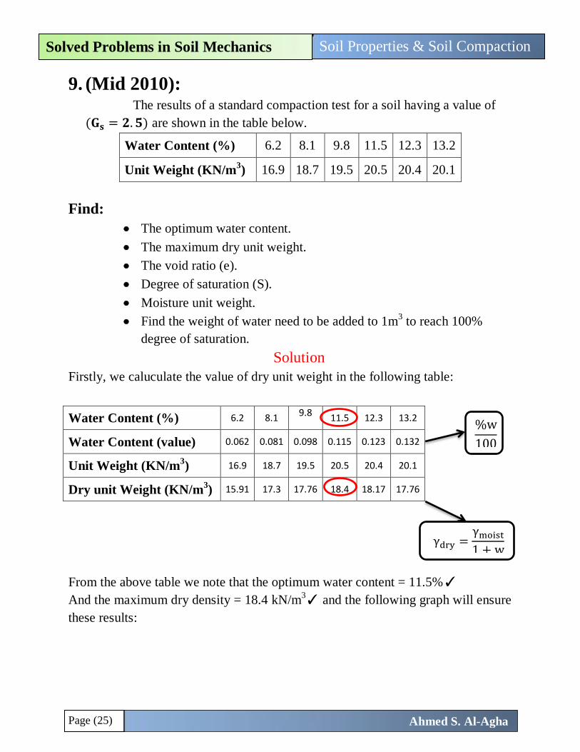
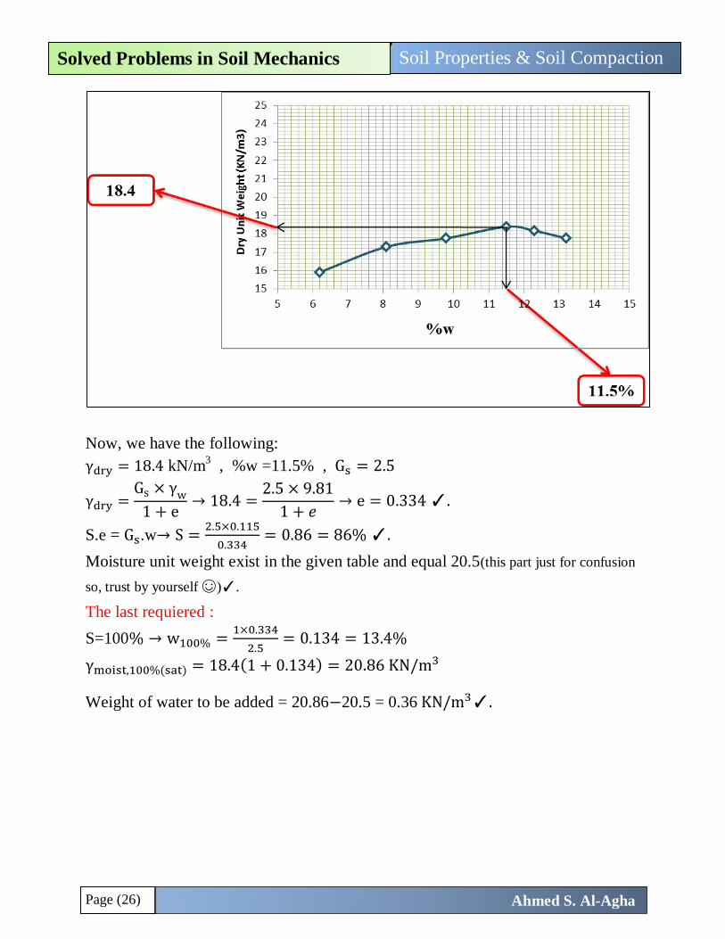
9. (Mid 2010): The results of a standard compaction test for a soil having a value of
(𝐆𝐬 = 𝟐. 𝟓) are shown in the table below.
Water Content (%) 6.2 8.1 9.8 11.5 12.3 13.2
Unit Weight (KN/m3) 16.9 18.7 19.5 20.5 20.4 20.1
Find:
The optimum water content.
The maximum dry unit weight.
The void ratio (e).
Degree of saturation (S).
Moisture unit weight.
Find the weight of water need to be added to 1m3 to reach 100%
degree of saturation.
Solution
Firstly, we caluculate the value of dry unit weight in the following table:
From the above table we note that the optimum water content = 11.5%✓ And the maximum dry density = 18.4 kN/m
3✓ and the following graph will ensure
these results:
Water Content (%) 6.2 8.1 9.8
11.5 12.3 13.2
Water Content (value) 0.062 0.081 0.098 0.115 0.123 0.132
Unit Weight (KN/m3) 16.9 18.7 19.5 20.5 20.4 20.1
Dry unit Weight (KN/m3) 15.91 17.3 17.76 18.4 18.17 17.76
%w
100
γdry =γmoist
1 + w
Page (26)
Soil Properties & Soil Compaction Solved Problems in Soil Mechanics
Ahmed S. Al-Agha
Now, we have the following:
γdry = 18.4 kN/m3 , %w =11.5% , Gs = 2.5
γdry =Gs × γw
1 + e→ 18.4 =
2.5 × 9.81
1 + 𝑒→ e = 0.334 ✓.
S.e = Gs.w→ S =2.5×0.115
0.334= 0.86 = 86% ✓.
Moisture unit weight exist in the given table and equal 20.5(this part just for confusion
so, trust by yourself ☺ )✓.
The last requiered :
S=100% → w100% =1×0.334
2.5= 0.134 = 13.4%
γmoist,100%(sat) = 18.4(1 + 0.134) = 20.86 KN/m3
Weight of water to be added = 20.86−20.5 = 0.36 KN/m3✓.
Page (27)
Soil Properties & Soil Compaction Solved Problems in Soil Mechanics
Ahmed S. Al-Agha
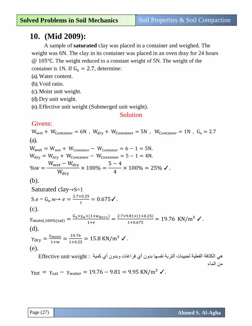
10. (Mid 2009): A sample of saturated clay was placed in a container and weighed. The
weight was 6N. The clay in its container was placed in an oven dray for 24 hours
@ 105℃. The weight reduced to a constant weight of 5N. The weight of the
container is 1N. If Gs = 2.7, determine:
(a). Water content.
(b). Void ratio.
(c). Moist unit weight.
(d). Dry unit weight.
(e). Effective unit weight (Submerged unit weight).
Solution
Givens:
Wwet + WContainer = 6N , Wdry + WContainer = 5N , WContainer = 1N , Gs = 2.7
(a).
Wwet = Wwet + WContainer − WContainer = 6 − 1 = 5N.
Wdry = Wdry + WContainer − WContainer = 5 − 1 = 4N.
%w = Wwet − Wdry
Wdry× 100% =
5 − 4
4× 100% = 25% ✓.
(b).
Saturated clay→S=1
S.e = Gs.w→ 𝑒 =2.7×0.25
1= 0.675✓.
(c).
γmoist,100%(sat) =Gs×𝛾𝑤×(1+𝑤@𝑠=1)
1+𝑒=
2.7×9.81×(1+0.25)
1+0.675= 19.76 KN/m3 ✓.
(d).
γdry =γmoist
1+w=
19.76
1+0.25= 15.8 KN/m3 ✓.
(e).
Effective unit weight : كثافة الفعلية لحبيبات التربة نفسها بدون أي فراغات وبدون أي كمية ال هي
من الماء
γEff. = γsat − γwater = 19.76 − 9.81 = 9.95 KN/m3 ✓.
Page (28)
Soil Properties & Soil Compaction Solved Problems in Soil Mechanics
Ahmed S. Al-Agha
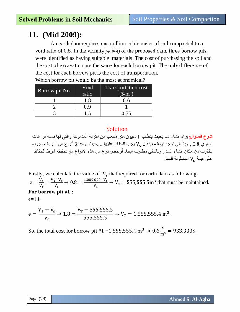
11. (Mid 2009): An earth dam requires one million cubic meter of soil compacted to a
void ratio of 0.8. In the vicinity(بالقرب) of the proposed dam, three borrow pits
were identified as having suitable materials. The cost of purchasing the soil and
the cost of excavation are the same for each borrow pit. The only difference of
the cost for each borrow pit is the cost of transportation.
Which borrow pit would be the most economical?
Borrow pit No. Void
ratio
Transportation cost
($/m3)
1 1.8 0.6
2 0.9 1
3 1.5 0.75
Solution
مليون متر مكعب من التربة المدموكة والتي لها نسبة فراغات 1يراد إنشاء سد بحيث يتطلب شرح السؤال:
أنواع من التربة موجودة 3يجب الحفاظ عليها ...بحيث يوجد Vs, وبالتالي توجد قيمة معينة ل 0.8تساوي
ذه األنواع مع تحقيقه شرط الحفاظ رخص نوع من هأيجاد إوبالتالي مطلوب , نشاء السد إبالقرب من مكان
المطلوبة للسد. Vsعلى قيمة
Firstly, we calculate the value of Vs that required for earth dam as following:
e =Vv
Vs=
VT−Vs
Vs→ 0.8 =
1,000,000−Vs
Vs→ Vs = 555,555.5m3 that must be maintained.
For borrow pit #1 :
e=1.8
e =VT − Vs
Vs→ 1.8 =
VT − 555,555.5
555,555.5→ VT = 1,555,555.4 m3.
So, the total cost for borrow pit #1 =1,555,555.4 m3 × 0.6$
m3= 933,333$ .
Page (29)
Soil Properties & Soil Compaction Solved Problems in Soil Mechanics
Ahmed S. Al-Agha
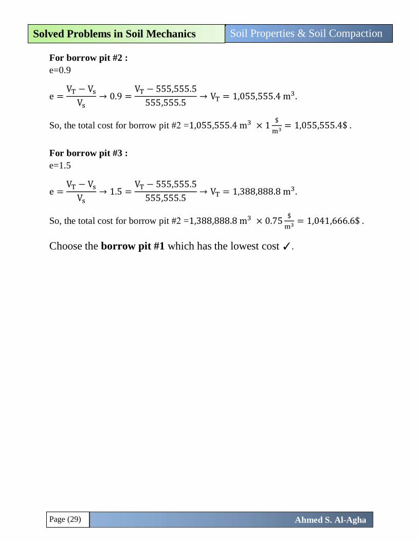
For borrow pit #2 :
e=0.9
e =VT − Vs
Vs→ 0.9 =
VT − 555,555.5
555,555.5→ VT = 1,055,555.4 m3.
So, the total cost for borrow pit #2 =1,055,555.4 m3 × 1$
m3= 1,055,555.4$ .
For borrow pit #3 :
e=1.5
e =VT − Vs
Vs→ 1.5 =
VT − 555,555.5
555,555.5→ VT = 1,388,888.8 m3.
So, the total cost for borrow pit #2 =1,388,888.8 m3 × 0.75$
m3= 1,041,666.6$ .
Choose the borrow pit #1 which has the lowest cost ✓.
Page (30)
Soil Properties & Soil Compaction Solved Problems in Soil Mechanics
Ahmed S. Al-Agha
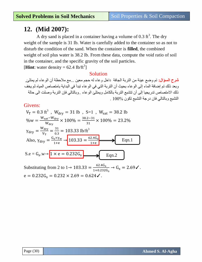
12. (Mid 2007): A dry sand is placed in a container having a volume of 0.3 ft
3. The dry
weight of the sample is 31 Ib. Water is carefully added to the container so as not to
disturb the condition of the sand. When the container is filled, the combined
weight of soil plus water is 38.2 Ib. From these data, compute the void ratio of soil
in the container, and the specific gravity of the soil particles.
[Hint: water density = 62.4 Ib/ft3]
Solution
تم وضع عينة من التربة الجافة داخل وعاء له حجم معين ...مع مالحظة أن الوعاء لم يمتلئ, شرح السؤال:
لى الوعاء بحيث أن التربة التي في الوعاء تبدأ في البداية بامتصاص المياه ثم يخف إضافة الماء إوبعد ذلك تم
الوعاء ..وبالتالي فإن التربة وصلت الى حالة ذلك االمتصاص تدريجيا إلى أن تتشبع التربة بالكامل ويمتلئ
. 100التشبع وبالتالي فان درجة التشبع تكون %
Givens:
VT = 0.3 ft3 , Wdry = 31 Ib , S=1 , Wsat = 38.2 Ib
%w = Wsat−Wdry
Wdry× 100% =
38.2−31
31× 100% = 23.2%
γdry =Wdry
VT=
31
0.3= 103.33 Ib/ft
3
Also, γdry =Gs×γw
1+e→ 103.33 =
62.4Gs
1+e
S.e = Gs.w→ 1 × e = 0.232Gs
Substituting from 2 to 1→ 103.33 =62.4Gs
1+0.232Gs→ Gs = 2.69✓.
e = 0.232Gs = 0.232 × 2.69 = 0.624✓.
Eqn.1
Eqn.2
Page (31)
Soil Properties & Soil Compaction Solved Problems in Soil Mechanics
Ahmed S. Al-Agha
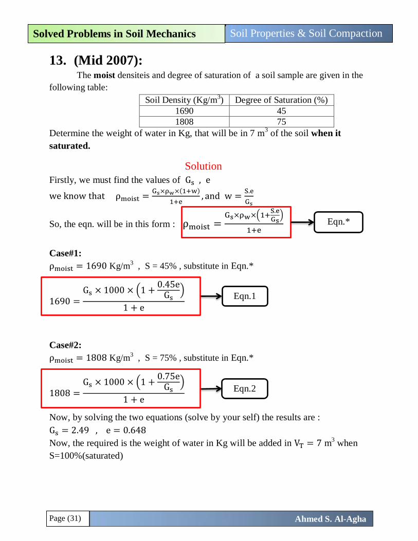
13. (Mid 2007): The moist densiteis and degree of saturation of a soil sample are given in the
following table:
Soil Density (Kg/m3) Degree of Saturation (%)
1690 45
1808 75
Determine the weight of water in Kg, that will be in 7 m3 of the soil when it
saturated.
Solution
Firstly, we must find the values of Gs , e
we know that ρmoist =Gs×ρw×(1+w)
1+e, and w =
S.e
Gs
So, the eqn. will be in this form : ρmoist =Gs×ρw×(1+
S.e
Gs)
1+e
Case#1:
ρmoist = 1690 Kg/m3 , S = 45% , substitute in Eqn.*
1690 =Gs × 1000 × (1 +
0.45eGs
)
1 + e
Case#2:
ρmoist = 1808 Kg/m3 , S = 75% , substitute in Eqn.*
1808 =Gs × 1000 × (1 +
0.75eGs
)
1 + e
Now, by solving the two equations (solve by your self) the results are :
Gs = 2.49 , e = 0.648
Now, the required is the weight of water in Kg will be added in VT = 7 m3 when
S=100%(saturated)
Eqn.*
Eqn.1
Eqn.2
Page (32)
Soil Properties & Soil Compaction Solved Problems in Soil Mechanics
Ahmed S. Al-Agha
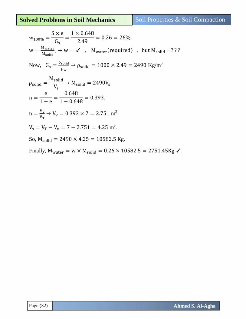
w100% =S × e
Gs=
1 × 0.648
2.49= 0.26 = 26%.
w =Mwater
Msolid, → w = ✓ , Mwater(required) , but Msolid =? ? ?
Now, Gs =ρsolid
ρw→ ρsolid = 1000 × 2.49 = 2490 Kg/m
3
ρsolid =Msolid
Vs→ Msolid = 2490Vs.
n =e
1 + e=
0.648
1 + 0.648= 0.393.
n =Vv
VT→ Vv = 0.393 × 7 = 2.751 m
3
Vs = VT − Vv = 7 − 2.751 = 4.25 m3.
So, Msolid = 2490 × 4.25 = 10582.5 Kg.
Finally, Mwater = w × Msolid = 0.26 × 10582.5 = 2751.45Kg ✓.
Page (33)
Soil Properties & Soil Compaction Solved Problems in Soil Mechanics
Ahmed S. Al-Agha
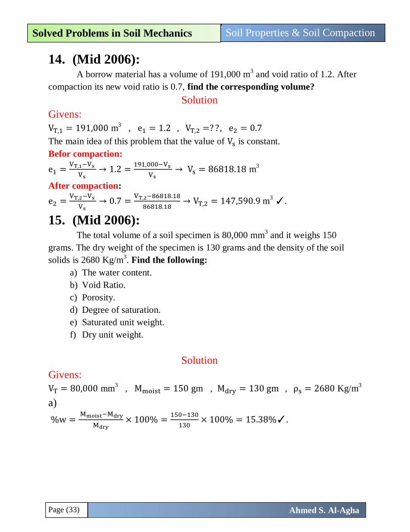
14. (Mid 2006): A borrow material has a volume of 191,000 m
3 and void ratio of 1.2. After
compaction its new void ratio is 0.7, find the corresponding volume?
Solution
Givens:
VT,1 = 191,000 m3 , e1 = 1.2 , VT,2 =? ?, e2 = 0.7
The main idea of this problem that the value of Vs is constant.
Befor compaction:
e1 =VT,1−Vs
Vs → 1.2 =
191,000−Vs
Vs → Vs = 86818.18 m
3
After compaction:
e2 =VT,2−Vs
Vs → 0.7 =
VT,2−86818.18
86818.18→ VT,2 = 147,590.9 m3
✓.
15. (Mid 2006): The total volume of a soil specimen is 80,000 mm
3 and it weighs 150
grams. The dry weight of the specimen is 130 grams and the density of the soil
solids is 2680 Kg/m3. Find the following:
a) The water content.
b) Void Ratio.
c) Porosity.
d) Degree of saturation.
e) Saturated unit weight.
f) Dry unit weight.
Solution
Givens:
VT = 80,000 mm3 , Mmoist = 150 gm , Mdry = 130 gm , ρs = 2680 Kg/m
3
a)
%w = Mmoist−Mdry
Mdry× 100% =
150−130
130× 100% = 15.38%✓.
Page (34)
Soil Properties & Soil Compaction Solved Problems in Soil Mechanics
Ahmed S. Al-Agha
b)
Gs =ρs
ρwater=
2680
1000= 2.68
VT = 80,000 mm3= 80,000 × 10−9 = 80 × 10−6 m
3
ρdry =Mdry
VT =
130×10−3
80×10−6= 1625 Kg/m
3
ρdry =Gs × ρw
1 + e→ 1625 =
2.68 × 1000
1 + e→ e = 0.649✓.
c)
n =e
1 + e=
0.649
1 + 0.649= 0.393✓.
d)
S.e=Gs. w → S =Gs.w
e=
2.68×0.1538
0.649= 0.635 = 63.5% ✓.
e)
S=1→ w100% =1×0.649
2.68= 0.242 = 24.2
γmoist,100%(sat) =Gs×γw×(1+w@s=1)
1+e=
2.68×9.81×(1+0.242)
1+0.649= 19.8 KN/m
3✓.
f)
ρdry = 1625 Kg/m3→ γdry = 1625 × 9.81 × 10−3 = 15.94 KN/m
3✓.
Page (35)
Soil Properties & Soil Compaction Solved Problems in Soil Mechanics
Ahmed S. Al-Agha
16. (Mid 2005): A sample of moist soil was found to have the following characteristics:
Volume 0.01456 m3 (as sampled)
Mass 25.74 Kg (as sampled)
22.10 Kg (after oven drying)
Specific gravity of solids: 2.69
Find the density, dry unit weight, void ratio, porosity, degree of saturation for
the soil.
What would be the moist unit weight when the degree of saturation is 80%?
Solution
Givens:
VT = 0.01456 m3 , Mmoist = 25.74 Kg , Mdry = 22.1 Kg , Gs = 2.69
(The first required is density that means moist and dry densities)
ρmoist =Mmoist
VT =
25.74
0.01456= 1767.56 Kg/m
3✓.
ρdry =Mdry
VT =
22.1
0.01456= 1517.86 Kg/m
3✓.
ρdry = 1517.86 Kg/m3→ γdry = 1517.86 × 9.81 × 10−3 = 14.89 KN/m
3✓.
γdry =Gs × γw
1 + e→ 14.89 =
2.69 × 9.81
1 + e→ e = 0.772 ✓.
S.e=Gs. w → w =? ?
ρmoist = ρdry(1 + w) → 1767.56 = 1517.86(1 + w) → w = 0.1645 = 16.45%
S =Gs. w
e=
2.69 × 0.1645
0.772= 0.573 = 57.3% ✓.
w =S. e
Gs=
0.8 × 0.772
2.69= 0.229 = 22.9%
γmoist =Gs×γw(1+𝑤)
1+e=
2.69×9.81×(1+0.229)
1+0.772= 18.3 KN/m
3✓.

Page (36)
Soil Properties & Soil Compaction Solved Problems in Soil Mechanics
Ahmed S. Al-Agha
17. (Final 2009): Dry soil with Gs = 2.7 is mixed with water to produce 20% water content
and compacted to produce a cylindrical sample of 40 mm diameter and 80mm long
with 5% air content. Calculate the following:
A- Mass of the mixed soil that will be required.
B- Void ratio of the sample.
C- Dry, moisture and saturated unit weight.
D- Amount of water to be added for full saturation.
Solution
Givens:
VT = volime of the cylindrical sample =π
4× (0.04)2 × 0.08 = 1.005 × 10⁻⁴ m
3
%w=20% , air content =5% , Gs = 2.7
Important Note: Air content = Vair
VT→ 0.05 =
Vair
VT→ Vair = 0.05VT.
A-
(Mmixed soil = Msolid) because the mixed soil is a dry soil and Mdry = Msolid
w = Mwater
Msolid→ Msolid =
Mwater
W=
Mwater
0.2→ Msolid = 5 Mwater
Gs =ρsolid
ρwater→ ρsolid = 1000 × 2.7 = 2700 Kg/m
3
ρsolid = Msolid
Vsolid→ Msolid = 2700 Vs
Vv = Vair + Vwater , and ρwater = Mwater
Vwater→ Vwater =
Mwater
ρwater, and Vv = VT − VS
→ VT − VS = 0.05VT + Mwater
ρwater but, VT = 1.005 × 10⁻⁴ and ρwater = 1000 Kg/m
3
So, VS = 0.95VT − Mwater
ρwater→ VS = 9.5 × 10⁻⁵ − 0.001 Mwater
Now, substitute in Eqn.2: → Msolid = 0.2565 − 2.7 Mwater → Substitute in Eq. 1
→ 0.2565 − 2.7 Mwater = 5 Mwater → Mwater =0.0333Kg.
Msolid = 5 × 0.0333 = 0.1665 Kg ✓.
Eqn.1
Eqn.2
Page (37)
Soil Properties & Soil Compaction Solved Problems in Soil Mechanics
Ahmed S. Al-Agha
B-
e = VV
Vs→ VS = 9.5 × 10⁻⁵ − 0.001 Mwater = VS = 9.5 × 10⁻⁵ − 0.001 × 0.0333
VS = 6.17 × 10⁻⁵ m3
VV = VT − VS = 1.005 × 10⁻⁴ − 6.17 × 10−5 = 3.88 × 10⁻⁵ m3
Then, e = 3.88×10⁻⁵
6.17×10−5= 0.628 ✓.
C-
γdry =Gs×γw
1+e=
2.7×9.81
1+0.628= 16.27 KN/m
3 ✓.
γmoist =Gs×γw(1+w)
1+e=
2.7×9.81(1+0.2)
1+0.628= 19.52 KN/m
3 ✓.
γsat =Gs×γw(1+
1×e
Gs)
1+e (Saturated → S = 1 → w =
1×e
Gs
γsat =2.7×9.81(1+
1×0.628
2.7)
1+0.628= 20.05 KN/m
3 ✓.
D-
Amount (KN/m3) = γsat−γmoist → Amount (KN) = (γsat−γmoist) × VT
Amount (KN) = (20.05−19.52) × 1.00510−4 = 5.326510−5KN ✓.
Amount (Kg) = 5.3265 × 10−5 ×1000
9.81= 5.4296 × 10⁻³ Kg✓.
Page (38)
Soil Properties & Soil Compaction Solved Problems in Soil Mechanics
Ahmed S. Al-Agha
18. A saturated soil sample has an initial total volume of 100 cm
3 and a moisture
content of 63%. The soil is then compressed so that the volume is reduced by 10
cm3 and the moisture content reduces to 53%. If the soil remains fully saturated,
calculate the Specific Gravity Gs.
Solution
Givens:
VT1 = 100 cm3 , w%1 = 63% , VT2 = 100 − 10 = 90 cm3 , w%2 = 53%
S1 = S2 = 100%, Gs =? ? ?
Calculate the void ration in each case (using given volumes):
e1 =VT,1 − Vs
Vs =
100 − Vs
Vs=
100
Vs− 1 → Eq. (1)
e2 =VT,2 − Vs
Vs =
90 − Vs
Vs=
90
Vs− 1 → Eq. (2)
Calculate the void ration in each case (using given volumes):
S1. e1 = Gs. w1 → 1 × e1 = 0.63Gs → e1 = 0.63 Gs → Eq. (3) S2. e2 = Gs. w2 → 1 × e2 = 0.53Gs → e2 = 0.53 Gs → Eq. (4)
By equating Eq.(1) and Eq.(3):
100
Vs− 1 = 0.63 Gs → Gs =
158.73
Vs− 1.587 → Eq. (5)
By equating Eq.(1) and Eq.(3):
90
Vs− 1 = 0.53 Gs → Gs =
169.81
Vs− 1.887 → Eq. (6)
Now, by equating Eq.(5) and Eq.(6):
158.73
Vs− 1.587 =
169.81
Vs− 1.887 = (multiply each side by Vs) →→
158.73 − 1.587Vs = 169.81 − 1.887 Vs → Vs = 36.93 cm3
Now to calculate Gs Substitute in Eq.(5) or Eq.(6):
Gs =158.73
Vs− 1.587 = Gs =
158.73
36.93− 1.587 = 2.71 ✓.
OR Gs =169.81
Vs− 1.887 = Gs =
169.81
36.93− 1.887 = 2.71✓.
Page (39)
Soil Properties & Soil Compaction Solved Problems in Soil Mechanics
Ahmed S. Al-Agha
19. Moist clayey soil has initial void ratio of 1.5, dry mass of 80gm, and specific
gravity of solid particles of 2.5.The sample is exposed to atmosphere so that the
sample volume decrease to one half of its initial volume . Calculate the following:
a) The new void ratio.
b) Mass of water if degree of saturation became 25 %.
Solution
Givens:
e1 = 1.5 , Mdry = Msolid = 80gm , Gs = 2.5 , VT,2 = 0.5VT,1
a)
Firstly, we must calculate the value of VT that must be the same in each case.
e1 =VT,1−Vs
Vs → 1.5 =
VT,1−Vs
Vs , VT,1 =? ? ?
ρdry =Mdry
VT,1=
Gs×ρw
1+e1→
0.08
VT,1=
2.5×1000
1+1.5→ VT,1 = 8 × 10⁻⁵m
3.
So, 1.5 =8×10⁻⁵−Vs
Vs→ Vs = 3.2 × 10⁻⁵ m
3.
Now, VT,2 = 0.5 × 8 × 10−5 = 4 × 10⁻⁵ m3.
e2 =VT,2 − Vs
Vs =
4 × 10⁻⁵ − 3.2 × 10⁻⁵
3.2 × 10−5 = 0.25 ✓.
b)
e = 0.25 , S=25% , Gs = 2.5
S.e = Gs. w → w =0.25×0.25
2.5= 0.025 = 2.5%.
w =Mwater
Msolid→ Mwater = 0.025 × 0.08 = 2 × 10⁻³Kg = 2gm ✓.
Page (40)
Soil Properties & Soil Compaction Solved Problems in Soil Mechanics
Ahmed S. Al-Agha
20.
Soil has been compacted in an embankment at a bulk unit weight of 2.15 t/m3
And water content of 12% , the solid particles of soil having specific gravity of 2.65.
a) Calculate the dry unit weight, degree of saturation, and air content.
b) Would it possible to compact the above soil at a water content of 13.5% to a dry
unit weight of 2 t/m3.
Solution
Givens:
γbulk = γmoist = 2.15 t/m3 = 2.15 × 9.81 = 21.0915 KN/m
3 (assume
g=9.81m/s2)
%w=12% , Gs = 2.65
a)
γdry =γmoist
1+w=
21.0915
1+0.12= 18.83 KN/m
3✓.
γdry =Gs × γw
1 + e→ 18.83 =
2.65 × 9.81
1 + e→ e = 0.38.
S.e = Gs. w → S =2.65×0.12
0.38= 0.837 = 83.7% ✓.
Air content = Vair
VT=? ?
Vv = Vair + Vwater
Vv = VT − VS
w = Wwater
Wsolid→ Wwater = 0.12 Wsolid
Gs =γsolid
γwater→ γsolid =
WS
VS→ Gs =
WS
VS × γwater→ WS = Gs × VS × γwater
Substitute in Eqn. 1 → Wwater = 0.12 × 2.65 × 9.81 × VS → Wwater = 3.12 VS
Vwater = Wwater
γwater→ Vwater =
3.12 VS
9.81= 0.318 VS
γdry = 18.83 = WS
VT=
𝐺𝑠 ×VS×γwater
VT→ VS = 0.7243 VT
→ Vwater = 0.318 × 0.7243 VT = 0.23 VT
Eqn.∗
Page (41)
Soil Properties & Soil Compaction Solved Problems in Soil Mechanics
Ahmed S. Al-Agha
Substitute in Eqn.*
VT − VS = Vair + Vwater
→ VT − 0.7243 VT = Vair + 0.23 VT (Dividing by VT)
→ 1 − 0.7243 =Vair
VT+ 0.23 →
Vair
VT= 0.0457 = 4.57% (Air content) ✓.
b)
%w =13.5% , γdry = 2 t/m3 = 2 × 9.81 = 19.62 KN/m
3(need to check)
If γZ.A.V > 19.62 → Ok , else → Not Ok.
γZ.A.V =Gs × γw
1 + emin→ emin =
Gs. w
Smax=
2.65 × 0.135
1= 0.3577
γZ.A.V =2.65×9.81
1+0.3577= 19.147 KN/m
3 <19.62 → Not possible✓.
Because the value of γZ.A.V is the maximum value of dry unit weight can be reach.
Another solution:
It’s supposed that the value of (e) must be greater than the value of (emin)
emin =Gs. w
Smax=
2.65 × 0.135
1= 0.3577
γdry =Gs × γw
1 + e→ 19.62 =
2.65 × 9.81
1 + e→ e = 0.325 < emin → Not possible✓.
Page (42)
Soil Properties & Soil Compaction Solved Problems in Soil Mechanics
Ahmed S. Al-Agha
21.
A specimen of soil was immersed in mercury. The mercury which came out
was collected and it’s weight was 290gm. The sample was oven dreid and it’s
weight became 30.2gm. if the specific gravity was 2.7 and weight of soil in natural
state was 34.6gm. Determine :
a) Tge void ratio,and porosity.
b) Water content of the original sample.
c) Degree of saturation of the original sample.
[Hint: the dnsity of mercury is 13.6 gm/cm3]
Solution
Givens:
Mmer.(came out) = 290gm , Mdry = 30.2gm , Mwet = 34.6gm , Gs = 2.7
Archimedes Law: The volume of specimen equal the voulme of liquid came out.
VT =Mmer
𝜌𝑚𝑒𝑟=
290
13.6= 21.32 cm
3= 21.32 × 10⁻⁶ m3.
a)
ρdry =Mdry
VT=
30.2×10⁻³
21.32×10−6= 1416.51 Kg/m
3
ρdry =Gs × ρw
1 + e→ 1416.51 =
2.7 × 1000
1 + e→ e = 0.906✓.
n =e
1 + e=
0.906
0.906 + 1= 0.475✓.
b)
%w = Mmoist − Mdry
Mdry× 100% =
34.6 − 30.2
30.2× 100% = 14.57%✓.
c)
S.e = Gs. w → S =2.7×0.1457
0.906= 0.4342 = 43.42%✓.
Page (43)
Soil Properties & Soil Compaction Solved Problems in Soil Mechanics
Ahmed S. Al-Agha
22. (Important)
The in-situ(field) moisture content of a soil is 18% and it’s moisture unit
weight is 105 pcf (Ib/ft3). The specific gravity of soil solids is 2.75. This soil is to
be excavated and transported to a construction site ,and then compacted to a
minimum dry weight of 103.5 pcf at a moisture content of 20 %.
a) How many cubic yards of excavated soil are needed to produce 10,000 yd3of
compacted fill?
b) How many truckloads are needed to transprt the excavated soil if each truck can
carry 20 tons?
[ Hint: 1ton = 2000Ib , 1yd3=27ft
3 , γw = 62.4pcf ] (I advise you to remember these units)
Solution
Givens:
For excavated soil (in-situ soil)
%w=18% , γmoist = 105 pcf , Gs = 2.75
For soil in the constrction site
%w=20% , γdry = 103.5 pcf , Gs = 2.75
نا عينة تربة في موقع معين وبمواصفات معينة ..حيث أنه يراد استخدام هذه التربة توجد لديشرح السؤال:
نشاءات..بالتالي سوف يتم حفر هذه التربة ونقلها في عربات وعند وصولها لموقع إلفي موقع معين ألعمال ا
Vs بقا أن قيمةنشاء سوف يتم دمكها وبالتالي سوف تتغير بعض خصائصها ...لكن دائما وأبدا كما ذكرنا ساإلا
ن الحبيبات الصلبة ال يتغير حجمها أبدا .ألتبقى ثابتة ..Ws تبقى ثابتة وأيضا قيمة
a)
VT,excavated soil =? ? , VT,constrction site soil = 10,000 yd3
For constrction site soil ∶
γdry =Gs × γw
1 + e→ 103.5 =
2.75 × 62.4
1 + e→ e = 0.658
e =VT−Vs
Vs→ 0.658 =
10,000−Vs
Vs→ Vs = 6031.36 yd
3 (That must be maintained)
Now, for excavated soil ∶
γmoist =Gs × γw(1 + w)
1 + e→ 105 =
2.75 × 62.4 × (1 + 0.18)
1 + e→ e = 0.9284
e =VT−Vs
Vs→ 0.9284 =
VT−6031.36
6031.36→ VT = 11,631.4 yd
3 ✓.

Page (44)
Soil Properties & Soil Compaction Solved Problems in Soil Mechanics
Ahmed S. Al-Agha
b) To find the number of trucks to transport the excavated soil we need two things:
- The total volume of excavated soil (in part a we calculate it =11,631.4 yd3)
- The total volume of each truck.
Each truck can carry 20 tons of excavated soil ….we want to convert this weight to
volume as following:
For each truck:
γmoist =Wmoist
VT→ VT,truck =
Wmoist,truck
γmoist,excavated soil=
(20ton×2000)Ib
105= 380.95 ft3
.
VT,truck = 380.95 ft3 = 380.95
27= 14.1 yd
3
So, # of trucks =VT,excavated soil
VT,truck=
11,631.4
14.1= 824.9 truck ✓.
Don’t say 825 because you have only 90 % (0.9) of the truck.
Page (45)
Soil Properties & Soil Compaction Solved Problems in Soil Mechanics
Ahmed S. Al-Agha
23. (Important)
An embankment for a highway 30 m wide and 1.5 m thick is to be
constructed from sandy soil, trucked in from a borrow pit .The water content of the
sandy soil in the borrow pit is 15% and its void ratio is 0.69. Specifications require
the embankment to compact to a dry weight of 18 KN/m3. Determine- for 1 km
length of embankment-the following:
a) The dry unit weight of sandy soil from the borrow pit to construct the
embankment, assuming that Gs = 2.7.
b) The number of 10 m3 truckloads of sandy soil required to construct the
embankment.
c) The weight of water per truck load of sandy soil.
d) The degree of saturation of the in-situ sandy soil.
Solution
Givens:
For borrow pit (in-situ soil)
%w=15% , e = 0.69 , Gs = 2.7
For embankment soil
VT = 30 × 1.5 × 1000 = 45,000 m3 , γdry = 18 KN/m3 , Gs = 2.7
ائه بتربة لها خواص معينة حيث أن هذه التربة يتم إحضارها نشإيوجد لدينا سد رملي مراد شرح السؤال:
والتي لها خواص معينة حيث سيتم نقلها الى مكان السد عن طريق borrow pit)من أماكن مخصصة لها )
نه مهما تم دمك التربة فان حجم تكون نفسها في كال الحالتين وذلك أل Vs شاحنات ..ومن المعروف أن قيمة
الصلبة ال يتغير.الحبيبات
a)
γdry =Gs×γw
1+e=
2.7×9.81
1+0.69= 15.67 KN/m
3.
b)
VT,truck = 10 m3 but VT,borrow pit soil =? ?
For embankment soil:
γdry =Gs × γw
1 + e→ 18 =
2.7 × 9.81
1 + e→ e = 0.4715.
e =VT−Vs
Vs→ 0.4715 =
45,000−Vs
Vs→ Vs = 30,581 m
3 (That must be maintained)
Page (46)
Soil Properties & Soil Compaction Solved Problems in Soil Mechanics
Ahmed S. Al-Agha
Now, for borrow pit soil:
e =VT−Vs
Vs→ 0.69 =
VT−30,581
30,581→ VT,borrow pit soil = 51,682 m
3.
So, # of trucks =VT,borrow pit soil
VT,truck=
51,682
10= 5168.2 truck ✓.
c)
For each truck → VT,truck = 10 m3
γdry = 15.67 KN/m3 for borrow pit soil
Now, γdry =Wdry
VT→ for each truck → Wdry,truck = γdry × VT,truck
→ Wdry,truck = 10 × 15.67 = 156.7 KN.
%w=Wwater
Wdry→ Wwater,truck = 156.7 × 0.15 = 23.5 KN✓.
d)
S.e=Gs. w → S =2.7×.15
0.69= 0.587 = 58.7%✓.
Page (47)
Soil Properties & Soil Compaction Solved Problems in Soil Mechanics
Ahmed S. Al-Agha
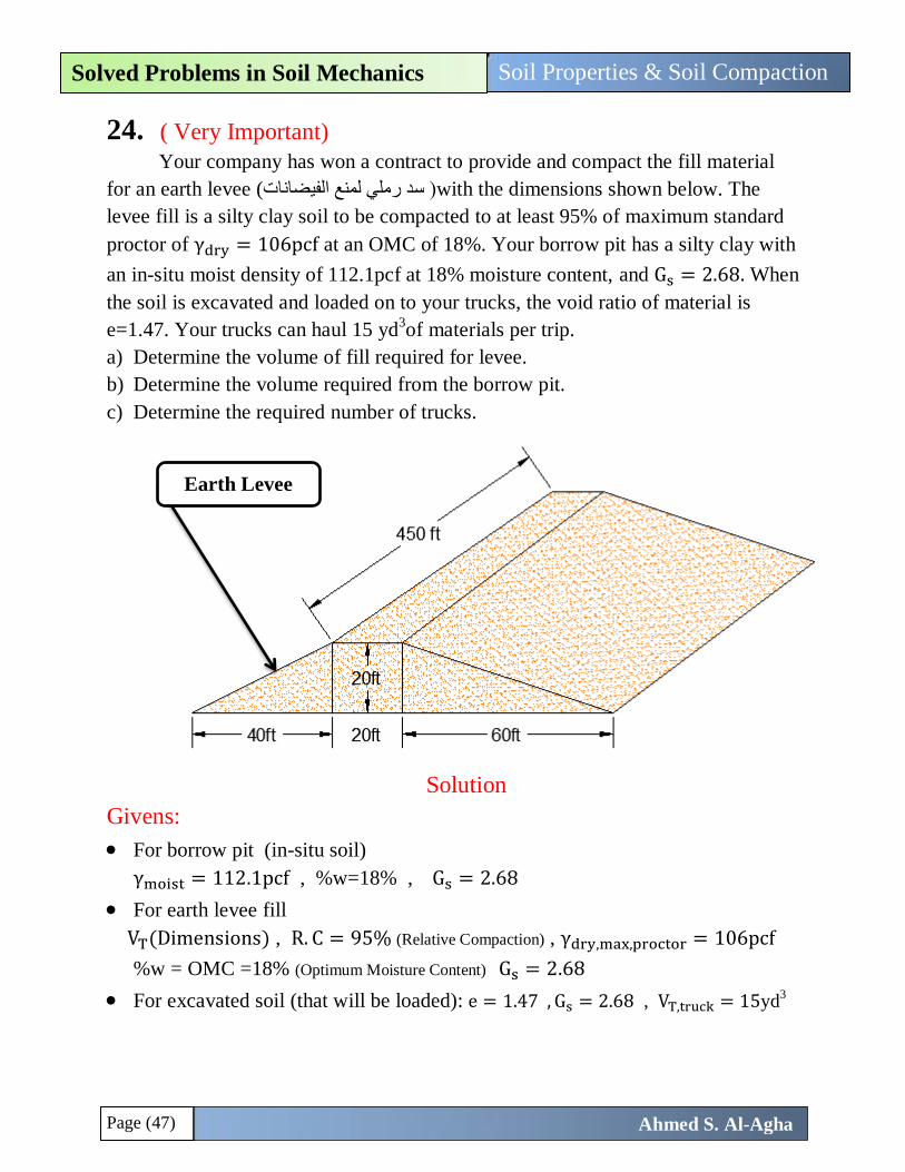
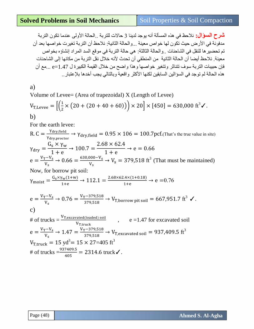
24. ( Very Important)
Your company has won a contract to provide and compact the fill material
for an earth levee (سد رملي لمنع الفيضانات (with the dimensions shown below. The
levee fill is a silty clay soil to be compacted to at least 95% of maximum standard
proctor of γdry = 106pcf at an OMC of 18%. Your borrow pit has a silty clay with
an in-situ moist density of 112.1pcf at 18% moisture content, and Gs = 2.68. When
the soil is excavated and loaded on to your trucks, the void ratio of material is
e=1.47. Your trucks can haul 15 yd3of materials per trip.
a) Determine the volume of fill required for levee.
b) Determine the volume required from the borrow pit.
c) Determine the required number of trucks.
Solution
Givens:
For borrow pit (in-situ soil)
γmoist = 112.1pcf , %w=18% , Gs = 2.68
For earth levee fill
VT(Dimensions) , R. C = 95% (Relative Compaction) , γdry,max,proctor = 106pcf
%w = OMC =18% (Optimum Moisture Content) Gs = 2.68
For excavated soil (that will be loaded): e = 1.47 , Gs = 2.68 , VT,truck = 15yd3
Earth Levee
Page (48)
Soil Properties & Soil Compaction Solved Problems in Soil Mechanics
Ahmed S. Al-Agha
حاالت للتربة ..الحالة األولى عندما تكون التربة 3نالحظ في هذه المسألة أنه يوجد لدينا شرح السؤال:
نالحظ أن التربة تغيرت خواصها بعد أن : مدفونة في األرض حيث تكون لها خواص معينة ...والحالة الثانية
هي حالة التربة في موقع السد المراد إنشاؤه بخواص :ت ..والحالة الثالثةتم تحضيرها للنقل في الشاحنا
من المنطقي أن تحدث ألنه خالل نقل التربة من مكانها إلى الشاحنات معينة. نالحظ أيضا أن الحالة الثانية
.مع أن .. e=1.47فإن حبيبات التربة سوف تتناثر وتتغير خواصها وهذا واضح من خالل القيمة الكبيرة ل
..بإلعتبارهذه الحالة لم توجد في السؤالين السابقين لكنها األكثر واقعية وبالتالي يجب أخدها
a)
Volume of Levee= (Area of trapezoidal) X (Length of Levee)
VT,Levee = [(1
2× (20 + (20 + 40 + 60))) × 20] × [450] = 630,000 ft
3✓.
b) For the earth levee:
R. C =γdry,field
γdry,proctor→ γdry,field = 0.95 × 106 = 100.7pcf.(That’s the true value in site)
γdry =Gs × γw
1 + e→ 100.7 =
2.68 × 62.4
1 + e→ e = 0.66
e =VT−Vs
Vs→ 0.66 =
630,000−Vs
Vs→ Vs = 379,518 ft
3 (That must be maintained)
Now, for borrow pit soil:
γmoist =Gs×γw(1+w)
1+e→ 112.1 =
2.68×62.4×(1+0.18)
1+e→ e =0.76
e =VT−Vs
Vs→ 0.76 =
VT−379,518
379,518→ VT,borrow pit soil = 667,951.7 ft
3 ✓.
c)
# of trucks = VT,excavated(loaded) soil
VT,truck , e =1.47 for excavated soil
e =VT−Vs
Vs→ 1.47 =
VT−379,518
379,518→ VT,excavated soil = 937,409.5 ft
3
VT,truck = 15 yd3= 15 × 27=405 ft
3
# of trucks =937409.5
405= 2314.6 truck✓.
Chapter (5)
Classification of Soil
Page (50)
Classification of Soil Solved Problems in Soil Mechanics
Ahmed S. Al-Agha
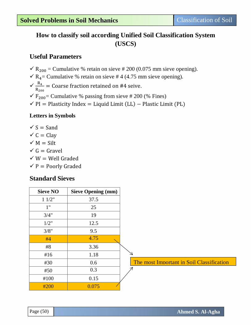
How to classify soil according Unified Soil Classification System
(USCS)
Useful Parameters
R200 = Cumulative % retain on sieve # 200 (0.075 mm sieve opening).
R4= Cumulative % retain on sieve # 4 (4.75 mm sieve opening).
R4
R200= Coarse fraction retained on #4 seive.
F200= Cumulative % passing from sieve # 200 (% Fines)
PI = Plasticity Index = Liquid Limit (LL) − Plastic Limit (PL)
Letters in Symbols
S = Sand
C = Clay
M = Silt
G = Gravel
W = Well Graded
P = Poorly Graded
Standard Sieves
Sieve NO Sieve Opening (mm)
1 1/2" 37.5
1" 25
3/4" 19
1/2" 12.5
3/8" 9.5
#4 4.75
#8 3.36
#16 1.18
#30 0.6
#50 0.3
#100 0.15
#200 0.075
The most Important in Soil Classification
Page (51)
Classification of Soil Solved Problems in Soil Mechanics
Ahmed S. Al-Agha
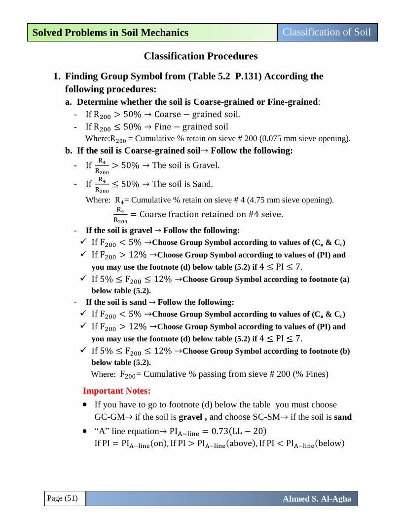
Classification Procedures
1. Finding Group Symbol from (Table 5.2 P.131) According the
following procedures:
a. Determine whether the soil is Coarse-grained or Fine-grained:
- If R200 > 50% → Coarse − grained soil.
- If R200 ≤ 50% → Fine − grained soil
Where:R200 = Cumulative % retain on sieve # 200 (0.075 mm sieve opening).
b. If the soil is Coarse-grained soil→ Follow the following:
- If R4
R200> 50% → The soil is Gravel.
- If R4
R200≤ 50% → The soil is Sand.
Where: R4= Cumulative % retain on sieve # 4 (4.75 mm sieve opening).
R4
R200= Coarse fraction retained on #4 seive.
- If the soil is gravel → Follow the following:
If F200 < 5% →Choose Group Symbol according to values of (Cu & Cc)
If F200 > 12% →Choose Group Symbol according to values of (PI) and
you may use the footnote (d) below table (5.2) if 4 ≤ PI ≤ 7.
If 5% ≤ F200 ≤ 12% →Choose Group Symbol according to footnote (a)
below table (5.2).
- If the soil is sand → Follow the following:
If F200 < 5% →Choose Group Symbol according to values of (Cu & Cc)
If F200 > 12% →Choose Group Symbol according to values of (PI) and
you may use the footnote (d) below table (5.2) if 4 ≤ PI ≤ 7.
If 5% ≤ F200 ≤ 12% →Choose Group Symbol according to footnote (b)
below table (5.2).
Where: F200= Cumulative % passing from sieve # 200 (% Fines)
Important Notes:
If you have to go to footnote (d) below the table you must choose
GC-GM→ if the soil is gravel , and choose SC-SM→ if the soil is sand
“A” line equation→ PIA−line = 0.73(LL − 20)
If PI = PIA−line(on), If PI > PIA−line(above), If PI < PIA−line(below)
Page (52)
Classification of Soil Solved Problems in Soil Mechanics
Ahmed S. Al-Agha
If you have to go to footnote (a) or (b) below the table → you have
more than one choice. How to find the correct symbol:
Assume that you have a gravel soil (for example) and 5% ≤ F200 ≤ 12%
You have to go to footnote (a) and you have the following choices:
(GW-GM, GW-GC, GP-GM, GP-GC) only one of them is true.
You will take each symbol and check it whether achieve the conditions or not
Firstly, you take GW-GM and check it …you must check each part of this
dual symbol as following:
GW: check it from table 5.2 according to values of (Cu & Cc)
GM: check it from table 5.2 according to value of (PI)
If one of them doesn’t achieve the condition you will reject the symbol
(GW-GM) and apply the same procedures on other symbols till one of the
symbols achieve the conditions (each part (from the 2 parts)) achieve the
conditions …only one symbol will achieve the conditions.
If you check GW (for example) in GW-GM, you don’t need to check it
another time in GW-GC ..Because it is the same check.
The same procedures above will apply if you have to go to footnote (b).
c. If the soil is Fine-grained soil→ Follow the following:
- According to value of liquid limit (LL) either LL< 50 or LL≥ 50.
- Always we deal with inorganic soil and don’t deal with organic soil.
- If LL< 50 , Choose Group Symbol according to values of (PI) and you may
use the footnote (e) below table (5.2) if 4 ≤ PI ≤ 7 .
- If LL≥ 50, Choose Group Symbol according to comparison between PI of
soil and PI from “A” line.
2. Finding group name:
a. From (figure 5.4 P.133) for Coarse (gravel & sand) and from (figure 5.5
P.143) for Fines (silt & clay).
b. To find group name easily you should know the following:
% Sand = R200 − R4 , % Gravel = R4
The value of (PI) >>>( in what range).
Comparison between PI & PIA−line to know (on, above or below A-line).
% Plus #200 sieve = % cumulative retained on #200 sieve = R200 .
Important Note: All values of R4, R200and F200 must depend on sieve analysis>>
must be cumulative (“R” increase with opening decrease and “F” decrease with
opening decrease).
Page (53)
Classification of Soil Solved Problems in Soil Mechanics
Ahmed S. Al-Agha
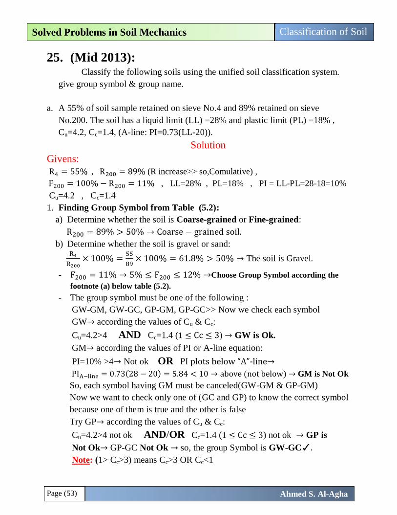
25. (Mid 2013): Classify the following soils using the unified soil classification system.
give group symbol & group name.
a. A 55% of soil sample retained on sieve No.4 and 89% retained on sieve
No.200. The soil has a liquid limit (LL) =28% and plastic limit (PL) =18% ,
Cu=4.2, Cc=1.4, (A-line: PI=0.73(LL-20)).
Solution
Givens:
R4 = 55% , R200 = 89% (R increase>> so,Comulative) ,
F200 = 100% − R200 = 11% , LL=28% , PL=18% , PI = LL-PL=28-18=10%
Cu=4.2 , Cc=1.4
1. Finding Group Symbol from Table (5.2):
a) Determine whether the soil is Coarse-grained or Fine-grained:
R200 = 89% > 50% → Coarse − grained soil.
b) Determine whether the soil is gravel or sand:
R4
R200× 100% =
55
89× 100% = 61.8% > 50% → The soil is Gravel.
- F200 = 11% → 5% ≤ F200 ≤ 12% →Choose Group Symbol according the
footnote (a) below table (5.2).
- The group symbol must be one of the following :
GW-GM, GW-GC, GP-GM, GP-GC>> Now we check each symbol
GW→ according the values of Cu & Cc:
Cu=4.2>4 AND Cc=1.4 (1 ≤ Cc ≤ 3) → GW is Ok.
GM→ according the values of PI or A-line equation:
PI=10% >4→ Not ok OR PI plots below “A”-line→
PIA−line = 0.73(28 − 20) = 5.84 < 10 → above (not below) → GM is Not Ok
So, each symbol having GM must be canceled(GW-GM & GP-GM)
Now we want to check only one of (GC and GP) to know the correct symbol
because one of them is true and the other is false
Try GP→ according the values of Cu & Cc:
Cu=4.2>4 not ok AND/OR Cc=1.4 (1 ≤ Cc ≤ 3) not ok → GP is
Not Ok→ GP-GC Not Ok → so, the group Symbol is GW-GC✓.
Note: (1> Cc>3) means Cc>3 OR Cc<1
Page (54)
Classification of Soil Solved Problems in Soil Mechanics
Ahmed S. Al-Agha
2. Finding Group Name from Figure (5.4):
% Sand = R200 − R4 = 89% − 55% = 34% > 15% →→ The group name is:
Well-graded gravel with clay and sand (or silty clay and sand) ✓.
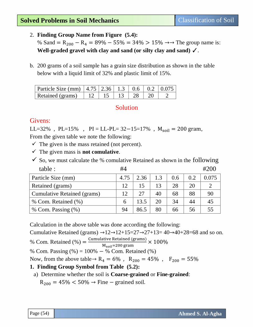
b. 200 grams of a soil sample has a grain size distribution as shown in the table
below with a liquid limit of 32% and plastic limit of 15%.
Particle Size (mm) 4.75 2.36 1.3 0.6 0.2 0.075
Retained (grams) 12 15 13 28 20 2
Solution
Givens:
LL=32% , PL=15% , PI = LL-PL= 32−15=17% , Msoil = 200 gram,
From the given table we note the following:
The given is the mass retained (not percent).
The given mass is not comulative.
So, we must calculate the % comulative Retained as shown in the following
table : #4 #200
Particle Size (mm) 4.75 2.36 1.3 0.6 0.2 0.075
Retained (grams) 12 15 13 28 20 2
Cumulative Retained (grams) 12 27 40 68 88 90
% Com. Retained (%) 6 13.5 20 34 44 45
% Com. Passing (%) 94 86.5 80 66 56 55
Calculation in the above table was done according the following:
Cumulative Retained (grams) →12→12+15=27→27+13= 40→40+28=68 and so on.
% Com. Retained (%) =Cumulative Retained (grams)
Msoil=200 gram× 100%
% Com. Passing (%) = 100% − % Com. Retained (%)
Now, from the above table→ R4 = 6% , R200 = 45% , F200 = 55%
1. Finding Group Symbol from Table (5.2):
a) Determine whether the soil is Coarse-grained or Fine-grained:
R200 = 45% < 50% → Fine − grained soil.
Page (55)
Classification of Soil Solved Problems in Soil Mechanics
Ahmed S. Al-Agha
b) Finding group symbol from the lower part of table (5.2):
LL= 32 < 50 & Inorganic soil → Classify according PI and “A”-line
→ PI = 17% > 7
→ PIA−line = 0.73(32 − 20) = 8.76 < 17 → above
So, PI > 7 AND Plots above “A”-line → Group Symbol is CL✓.
2. Finding Group Name from Figure (5.5):
The following parameters will be used:
LL=32 , PI=17and Plots above “A”-line , %plus No.200 = R200 = 45%
% Sand = R200 − R4 = 45 − 6 = 39% , %Gravel = R4 = 6%
Now, we find group name as following:
LL= 32 < 50 → Inorganic → PI > 7and Plots above “A”-line
→ CL → R200 = 45% > 30% → %Sand = 39% > %Gravel = 6%
→ %Gravel = 6% < 15% →→ Group Name is Sandy Lean Clay✓.
Page (56)
Classification of Soil Solved Problems in Soil Mechanics
Ahmed S. Al-Agha
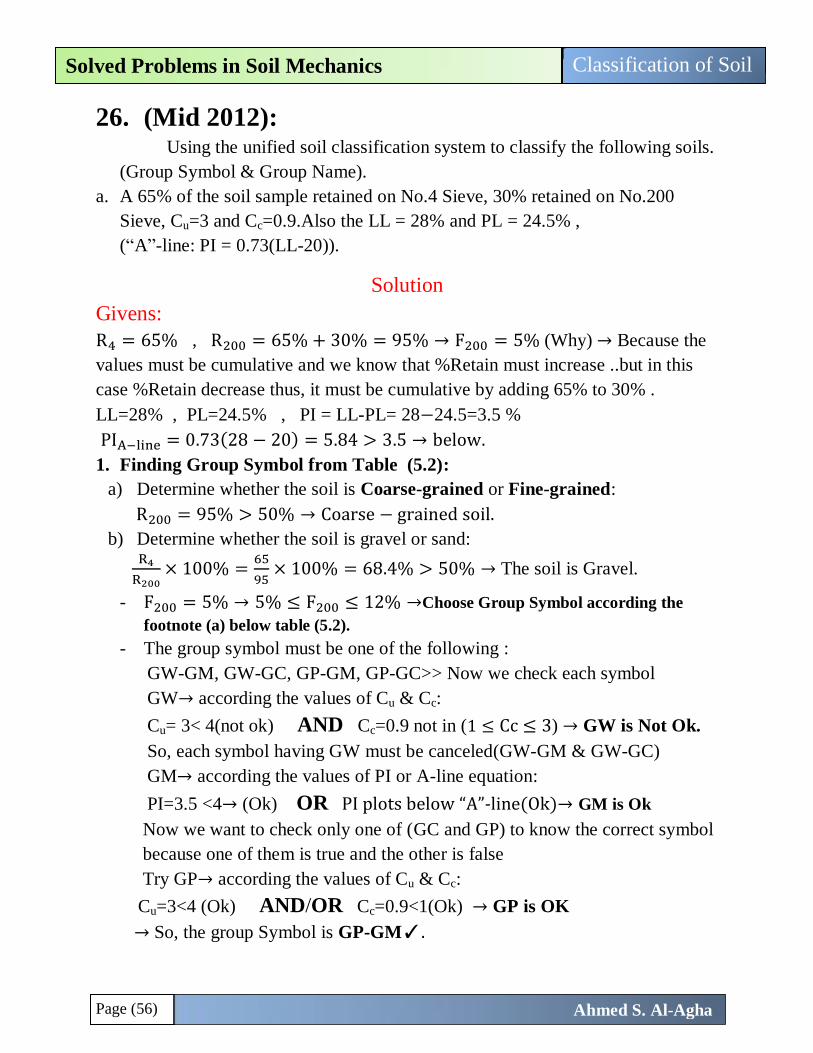
26. (Mid 2012): Using the unified soil classification system to classify the following soils.
(Group Symbol & Group Name).
a. A 65% of the soil sample retained on No.4 Sieve, 30% retained on No.200
Sieve, Cu=3 and Cc=0.9.Also the LL = 28% and PL = 24.5% ,
(“A”-line: PI = 0.73(LL-20)).
Solution
Givens:
R4 = 65% , R200 = 65% + 30% = 95% → F200 = 5% (Why) → Because the
values must be cumulative and we know that %Retain must increase ..but in this
case %Retain decrease thus, it must be cumulative by adding 65% to 30% .
LL=28% , PL=24.5% , PI = LL-PL= 28−24.5=3.5 %
PIA−line = 0.73(28 − 20) = 5.84 > 3.5 → below.
1. Finding Group Symbol from Table (5.2):
a) Determine whether the soil is Coarse-grained or Fine-grained:
R200 = 95% > 50% → Coarse − grained soil.
b) Determine whether the soil is gravel or sand: R4
R200× 100% =
65
95× 100% = 68.4% > 50% → The soil is Gravel.
- F200 = 5% → 5% ≤ F200 ≤ 12% →Choose Group Symbol according the
footnote (a) below table (5.2).
- The group symbol must be one of the following :
GW-GM, GW-GC, GP-GM, GP-GC>> Now we check each symbol
GW→ according the values of Cu & Cc:
Cu= 3< 4(not ok) AND Cc=0.9 not in (1 ≤ Cc ≤ 3) → GW is Not Ok.
So, each symbol having GW must be canceled(GW-GM & GW-GC)
GM→ according the values of PI or A-line equation:
PI=3.5 <4→ (Ok) OR PI plots below “A”-line(Ok)→ GM is Ok
Now we want to check only one of (GC and GP) to know the correct symbol
because one of them is true and the other is false
Try GP→ according the values of Cu & Cc:
Cu=3<4 (Ok) AND/OR Cc=0.9<1(Ok) → GP is OK
→ So, the group Symbol is GP-GM✓.
Page (57)
Classification of Soil Solved Problems in Soil Mechanics
Ahmed S. Al-Agha
2. Finding Group Name from Figure (5.4):
% Sand = R200 − R4 = 95% − 65% = 30% > 15% →→ The group name is:
Poorly graded gravel with silt and sand✓.
Now, as you see the classification is so easy, just you need some focusing, so I
will finish solving problems completely in this chapter , but I will explain some
ideas, and I give you the answer to solve the problems by yourself and check
your solution.
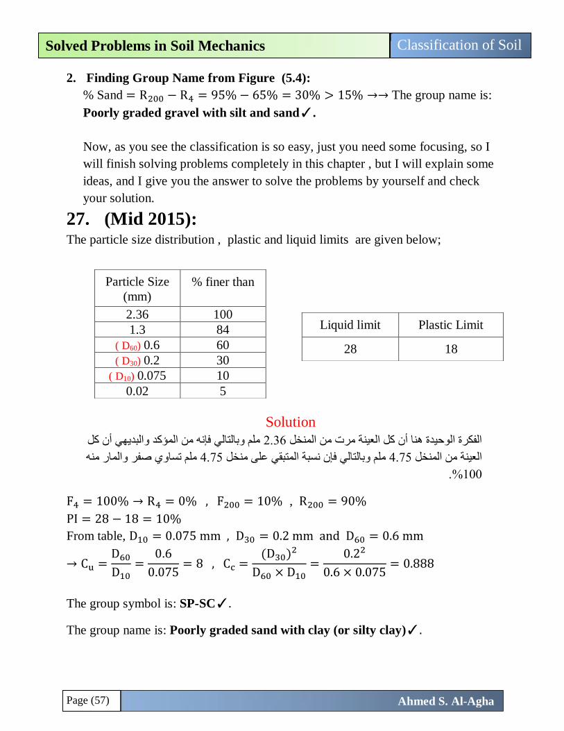
27. (Mid 2015): The particle size distribution , plastic and liquid limits are given below;
Solution
ملم وبالتالي فإنه من المؤكد والبديهي أن كل 2.36الفكرة الوحيدة هنا أن كل العينة مرت من المنخل
ملم تساوي صفر والمار منه 4.75ملم وبالتالي فإن نسبة المتبقي على منخل 4.75العينة من المنخل
100.%
F4 = 100% → R4 = 0% , F200 = 10% , R200 = 90%
PI = 28 − 18 = 10%
From table, D10 = 0.075 mm , D30 = 0.2 mm and D60 = 0.6 mm
→ Cu =D60
D10=
0.6
0.075= 8 , Cc =
(D30)2
D60 × D10=
0.22
0.6 × 0.075= 0.888
The group symbol is: SP-SC✓.
The group name is: Poorly graded sand with clay (or silty clay)✓.
Particle Size
(mm)
% finer than
2.36 100
1.3 84
( D60) 0.6 60
( D30) 0.2 30
( D10) 0.075 10
0.02 5
Liquid limit Plastic Limit
28 18
Page (58)
Classification of Soil Solved Problems in Soil Mechanics
Ahmed S. Al-Agha
28. (Mid 2011): a. 86% of a soil sample passed Sieve No.4 and retained on Sieve No.200. Also
given that: Coefficient of gradation=1 , Uniformity Coefficient = 3
Solution
من العينة , % 14وبالتالي تبقى عليه 4% من العينة مرت من المنخل رقم 86نالحظ أن :شرح السؤال
% التي 14..وبالتالي فإن ال 200كلها بقيت على المنخل رقم 4% التي مرت من المنخل رقم 86وأن ال
وبالتالي يصبح المتبقي على المنخل رقم 200سوف تبقى أيضا على المنخل رقم 4بقيت على المنخل رقم
المار منه فهو صفرا. % )ألن التجربة يجب أن تكون تراكمية( أما 100= 14+86يساوي 200
F4 = 86% → R4 = 14% , F200 = 0.0 , R200 = 100%
Coefficient of gradation = Cc=1 , Uniformity Coefficient = Cu= 3
The group symbol is: SP✓.
The group name is: Poorly graded sand✓.
b. A sieve analysis of a soil show that 97% of the soil passed sieve No.4 and 73%
passed sieve No.200. If the liquid limit of the soil is 62 and its plastic limit =34.
Solution
F4 = 97% → R4 = 3% , F200 = 73% , R200 = 27%
LL=62% , PL=34% , PI = LL-PL= 62−34=28 %
No idea in this question but you should be attention for the large value of LL
because it will be used when you finding group symbol.
The group symbol is: MH✓.
The group name is: Elastic silt with sand✓.
Page (59)
Classification of Soil Solved Problems in Soil Mechanics
Ahmed S. Al-Agha
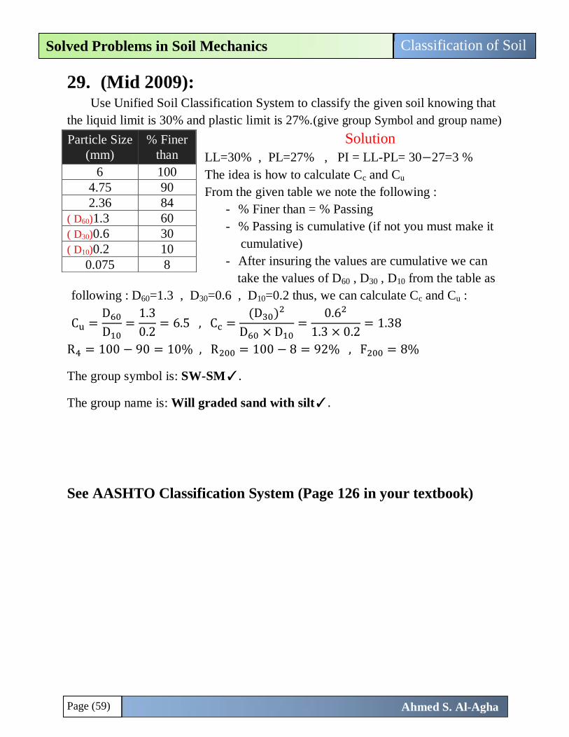
29. (Mid 2009): Use Unified Soil Classification System to classify the given soil knowing that
the liquid limit is 30% and plastic limit is 27%.(give group Symbol and group name)
Solution
LL=30% , PL=27% , PI = LL-PL= 30−27=3 %
The idea is how to calculate Cc and Cu
From the given table we note the following :
- % Finer than = % Passing
- % Passing is cumulative (if not you must make it
… cumulative)
- After insuring the values are cumulative we can
take the values of D60 , D30 , D10 from the table as
following : D60=1.3 , D30=0.6 , D10=0.2 thus, we can calculate Cc and Cu :
Cu =D60
D10=
1.3
0.2= 6.5 , Cc =
(D30)2
D60 × D10=
0.62
1.3 × 0.2= 1.38
R4 = 100 − 90 = 10% , R200 = 100 − 8 = 92% , F200 = 8%
The group symbol is: SW-SM✓.
The group name is: Will graded sand with silt✓.
See AASHTO Classification System (Page 126 in your textbook)
Particle Size
(mm)
% Finer
than
6 100
4.75 90
2.36 84
( D60)1.3 60
( D30)0.6 30
( D10)0.2 10
0.075 8

Chapter (7)
Soil Permeability
Page (61)
Soil Permeability Solved Problems in Soil Mechanics
Ahmed S. Al-Agha
Bernoulli’s Equation (for Soil):
Total Head = Pressure Head + Velocity Head + Elevation Head
htotal =u
γw+
v2
2g+ Z
u: pore water pressure
v: velocity of water through the soil
Z: vertical distance of a given point above or below a datum plane.
Notes:
Pressure head is also called “piezometric head”.
u = hpressure × γw.
The velocity of water through soil is very small (about 0.01→0.001)m/sec and
when the velocity is squared the value will be very small so, the velocity head
in Bernoulli’s equation should be canceled and the final form of bernoulli’s
equation will be : htotal =u
γw+ Z
The head loss that result from the movement of water through the soil (∆H)
can be expressed in a nondimensional form as:
i =∆H
L , where:
i = Hydraulic gradient (The head loss per unit length)
في التربة الماء لكل متر)أو أي وحدة طول( تتحركه head ال وهي تعبر عن مقدار الفقدان في
L = Total length of soil or soils that the water passes through it
Darcy’s Low: Darcy found that, there are proportional relationship between velocity (v) and
hydraulic gradient (i), this relationship still valid if the flow still laminar , and in
soil the velocity is small so, the flow is always laminar.
v ∝ i → v = k. i
K: Hydraulic conductivity of soil = Permeability of soil (m/sec)
Now, we know that: Q = V × A and v = k. i (Darcy’s low) →→→
Q = K. i. A
A: Cross sectional area that perpendicular to flow direction.
Page (62)
Soil Permeability Solved Problems in Soil Mechanics
Ahmed S. Al-Agha
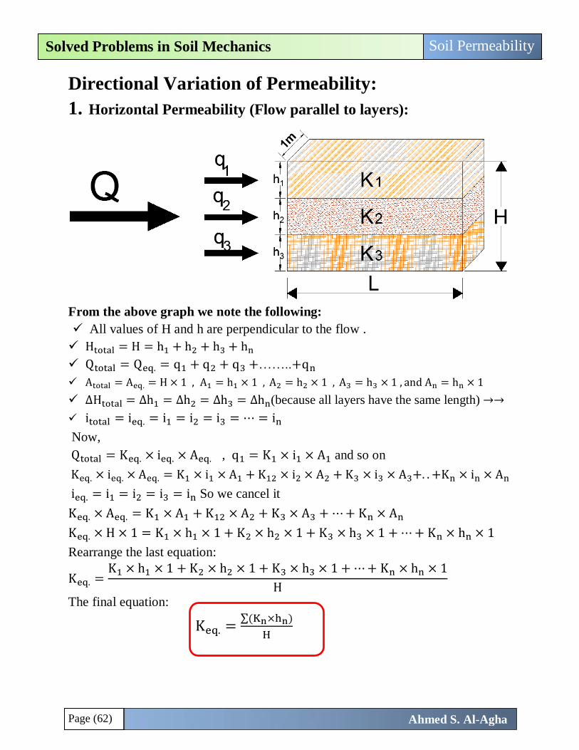
Directional Variation of Permeability:
1. Horizontal Permeability (Flow parallel to layers):
From the above graph we note the following:
All values of H and h are perpendicular to the flow .
Htotal = H = h1 + h2 + h3 + hn
Qtotal = Qeq. = q1 + q2 + q3 +……..+qn
Atotal = Aeq. = H × 1 , A1 = h1 × 1 , A2 = h2 × 1 , A3 = h3 × 1 , and An = hn × 1
∆Htotal = ∆h1 = ∆h2 = ∆h3 = ∆hn(because all layers have the same length) →→
itotal = ieq. = i1 = i2 = i3 = ⋯ = in
Now,
Qtotal = Keq. × ieq. × Aeq. , q1 = K1 × i1 × A1 and so on
Keq. × ieq. × Aeq. = K1 × i1 × A1 + K12 × i2 × A2 + K3 × i3 × A3+. . +Kn × in × An
ieq. = i1 = i2 = i3 = in So we cancel it
Keq. × Aeq. = K1 × A1 + K12 × A2 + K3 × A3 + ⋯ + Kn × An
Keq. × H × 1 = K1 × h1 × 1 + K2 × h2 × 1 + K3 × h3 × 1 + ⋯ + Kn × hn × 1
Rearrange the last equation:
Keq. =K1 × h1 × 1 + K2 × h2 × 1 + K3 × h3 × 1 + ⋯ + Kn × hn × 1
H
The final equation:
Keq. =∑(Kn×hn)
H
Page (63)
Soil Permeability Solved Problems in Soil Mechanics
Ahmed S. Al-Agha
2. Vertical Permeability (Flow perpendicular to layers):
From the above graph we note the following:
Htotal = H = h1 + h2 + h3 + hn
Qtotal = Qeq. = q1 = q2 = q3 =……..= qn
Atotal = Aeq. = L × 1 = A1 = A2 = A3 = ⋯ = An
∆Htotal = ∆h1 + ∆h2 + ∆h3 + ∆hn(because flow pass through each layer) →→
itotal = ieq. + i1 + i2 + i3 + ⋯ + in
Now,
qn = Kn ×∆hn
hn× An → ∆hn =
qn×hn
Kn× An
Qeq.×H
Keq.×Aeq.=
q1×h1
K1× A1+
q2×h2
K2× A2+
q3×h3
K3× A3+ ⋯ +
qn×hn
Kn× An (Q and A are the same→ cancel them)
H
Keq.=
h1
K1+
h2
K2+
h3
K3+ ⋯ +
hn
Kn→→ The final equation:
Keq. =H
h1K1
+h2K2
+h3K3
+⋯+hnKn
Note: All values of H and h are parallel to the flow
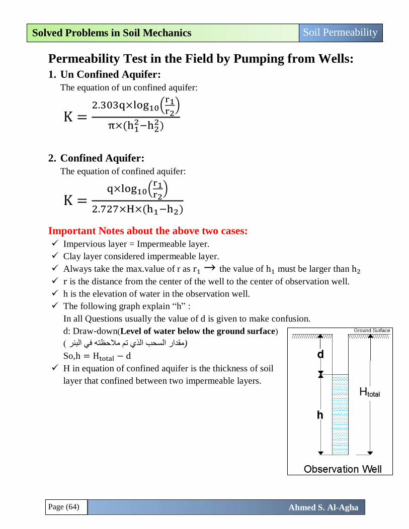
Page (64)
Soil Permeability Solved Problems in Soil Mechanics
Ahmed S. Al-Agha
Permeability Test in the Field by Pumping from Wells:
1. Un Confined Aquifer: The equation of un confined aquifer:
K =2.303q×log10(
r1r2
)
π×(h12−h2
2)
2. Confined Aquifer: The equation of confined aquifer:
K =q×log10(
r1r2
)
2.727×H×(h1−h2)
Important Notes about the above two cases:
Impervious layer = Impermeable layer.
Clay layer considered impermeable layer.
Always take the max.value of r as r1 → the value of h1 must be larger than h2
r is the distance from the center of the well to the center of observation well.
h is the elevation of water in the observation well.
The following graph explain “h” :
In all Questions usually the value of d is given to make confusion.
d: Draw-down(Level of water below the ground surface)
ه في البئرتمقدار السحب الذي تم مالحظ ( )
So,h = Htotal − d
H in equation of confined aquifer is the thickness of soil
layer that confined between two impermeable layers.
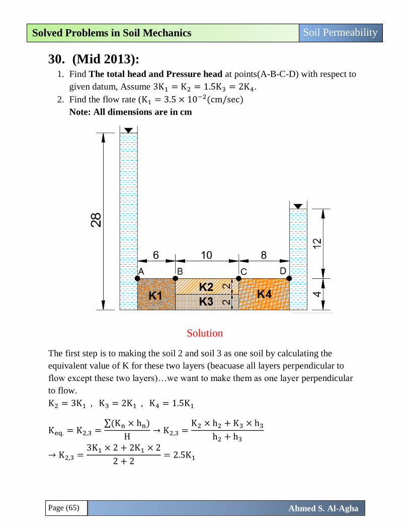
Page (65)
Soil Permeability Solved Problems in Soil Mechanics
Ahmed S. Al-Agha
30. (Mid 2013): 1. Find The total head and Pressure head at points(A-B-C-D) with respect to
given datum, Assume 3K1 = K2 = 1.5K3 = 2K4. 2. Find the flow rate (K1 = 3.5 × 10⁻²(cm/sec)
Note: All dimensions are in cm
Solution
The first step is to making the soil 2 and soil 3 as one soil by calculating the
equivalent value of K for these two layers (beacuase all layers perpendicular to
flow except these two layers)…we want to make them as one layer perpendicular
to flow.
K2 = 3K1 , K3 = 2K1 , K4 = 1.5K1
Keq. = K2,3 =∑(Kn × hn)
H→ K2,3 =
K2 × h2 + K3 × h3
h2 + h3
→ K2,3 =3K1 × 2 + 2K1 × 2
2 + 2= 2.5K1
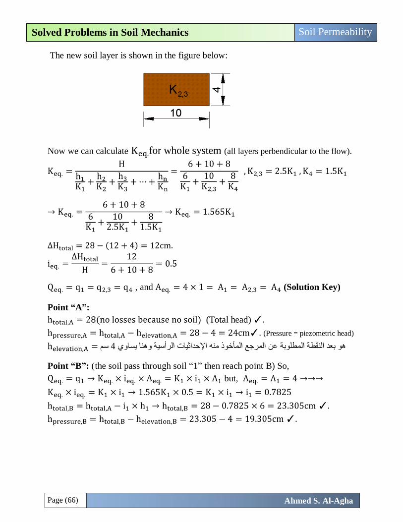
Page (66)
Soil Permeability Solved Problems in Soil Mechanics
Ahmed S. Al-Agha
The new soil layer is shown in the figure below:
Now we can calculate Keq.for whole system (all layers perbendicular to the flow).
Keq. =H
h1K1
+h2K2
+h3
K3+ ⋯ +
hnKn
=6 + 10 + 8
6K1
+10
K2,3+
8K4
, K2,3 = 2.5K1 , K4 = 1.5K1
→ Keq. =6 + 10 + 8
6K1
+10
2.5K1+
81.5K1
→ Keq. = 1.565K1
∆Htotal = 28 − (12 + 4) = 12cm.
ieq. =∆Htotal
H=
12
6 + 10 + 8= 0.5
Qeq. = q1 = q2,3 = q4 , and Aeq. = 4 × 1 = A1 = A2,3 = A4 (Solution Key)
Point “A”:
htotal,A = 28(no losses because no soil) (Total head) ✓.
hpressure,A = htotal,A − helevation,A = 28 − 4 = 24cm✓. (Pressure = piezometric head)
helevation,A = سم 4حداثيات الرأسية وهنا يساوي إلهو بعد النقطة المطلوبة عن المرجع المأخوذ منه ا
Point “B”: ( the soil pass through soil “1” then reach point B) So,
Qeq. = q1 → Keq. × ieq. × Aeq. = K1 × i1 × A1 but, Aeq. = A1 = 4 →→→
Keq. × ieq. = K1 × i1 → 1.565K1 × 0.5 = K1 × i1 → i1 = 0.7825
htotal,B = htotal,A − i1 × h1 → htotal,B = 28 − 0.7825 × 6 = 23.305cm ✓.
hpressure,B = htotal,B − helevation,B = 23.305 − 4 = 19.305cm ✓.
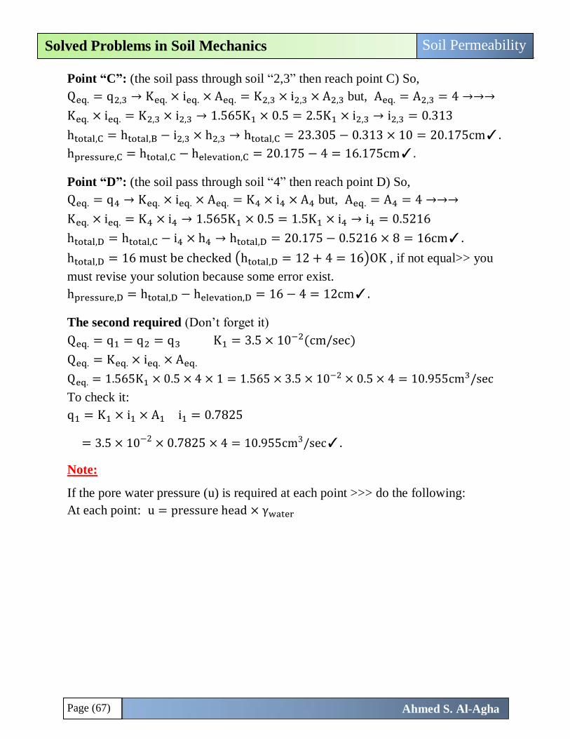
Page (67)
Soil Permeability Solved Problems in Soil Mechanics
Ahmed S. Al-Agha
Point “C”: (the soil pass through soil “2,3” then reach point C) So,
Qeq. = q2,3 → Keq. × ieq. × Aeq. = K2,3 × i2,3 × A2,3 but, Aeq. = A2,3 = 4 →→→
Keq. × ieq. = K2,3 × i2,3 → 1.565K1 × 0.5 = 2.5K1 × i2,3 → i2,3 = 0.313
htotal,C = htotal,B − i2,3 × h2,3 → htotal,C = 23.305 − 0.313 × 10 = 20.175cm✓.
hpressure,C = htotal,C − helevation,C = 20.175 − 4 = 16.175cm✓.
Point “D”: (the soil pass through soil “4” then reach point D) So,
Qeq. = q4 → Keq. × ieq. × Aeq. = K4 × i4 × A4 but, Aeq. = A4 = 4 →→→
Keq. × ieq. = K4 × i4 → 1.565K1 × 0.5 = 1.5K1 × i4 → i4 = 0.5216
htotal,D = htotal,C − i4 × h4 → htotal,D = 20.175 − 0.5216 × 8 = 16cm✓.
htotal,D = 16 must be checked (htotal,D = 12 + 4 = 16)OK , if not equal>> you
must revise your solution because some error exist.
hpressure,D = htotal,D − helevation,D = 16 − 4 = 12cm✓.
The second required (Don’t forget it)
Qeq. = q1 = q2 = q3 K1 = 3.5 × 10⁻²(cm/sec)
Qeq. = Keq. × ieq. × Aeq.
Qeq. = 1.565K1 × 0.5 × 4 × 1 = 1.565 × 3.5 × 10−2 × 0.5 × 4 = 10.955cm3/sec
To check it:
q1 = K1 × i1 × A1 i1 = 0.7825
= 3.5 × 10−2 × 0.7825 × 4 = 10.955cm3/sec✓.
Note:
If the pore water pressure (u) is required at each point >>> do the following:
At each point: u = pressure head × γwater
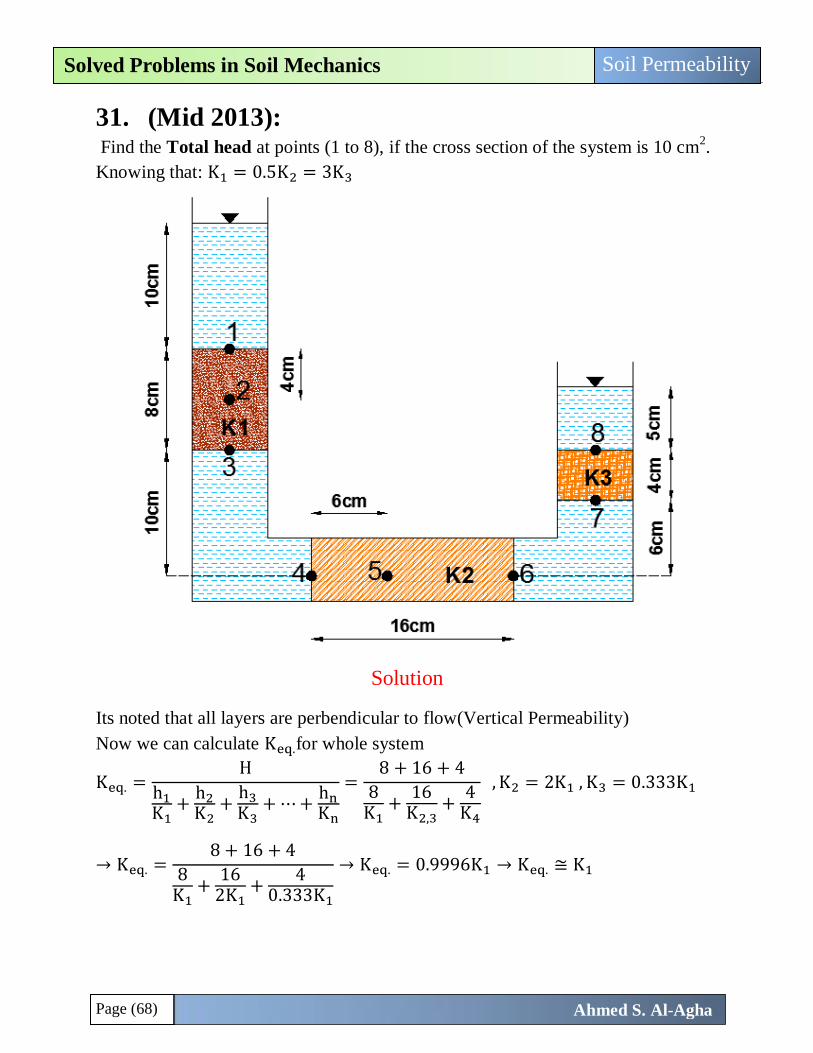
Page (68)
Soil Permeability Solved Problems in Soil Mechanics
Ahmed S. Al-Agha
31. (Mid 2013): Find the Total head at points (1 to 8), if the cross section of the system is 10 cm
2.
Knowing that: K1 = 0.5K2 = 3K3
Solution
Its noted that all layers are perbendicular to flow(Vertical Permeability)
Now we can calculate Keq.for whole system
Keq. =H
h1K1
+h2K2
+h3
K3+ ⋯ +
hnKn
=8 + 16 + 4
8K1
+16
K2,3+
4K4
, K2 = 2K1 , K3 = 0.333K1
→ Keq. =8 + 16 + 4
8K1
+16
2K1+
40.333K1
→ Keq. = 0.9996K1 → Keq. ≅ K1
Page (69)
Soil Permeability Solved Problems in Soil Mechanics
Ahmed S. Al-Agha
∆Htotal = (10 + 8 + 10) − (6 + 4 + 5) = 13cm.
ieq. =∆Htotal
H=
13
8 + 16 + 4= 0.4643
Qeq. = q1 = q2 = q3 , and Aeq. = 10cm2 = A1 = A2 = A3 (Solution Key)
Point “1”:
htotal,1 = 28(no losses because no soil) (Total head) ✓.
Point “2”: ( the soil pass through the mid of soil “1” then reach point 2) So,
Qeq. = q1 → Keq. × ieq. × Aeq. = K1 × i1 × A1 but, Aeq. = A1 = 10 →→→
Keq. × ieq. = K1 × i1 → K1 × 0.4643 = K1 × i1 → i1 = 0.4643
htotal,2 = htotal,1 − i1 × 4 → htotal,2 = 28 − 0.4643 × 4 = 26.1428cm✓.
Point “3”: ( the soil pass through all of soil “1” then reach point 3) So,
Qeq. = q1 → Keq. × ieq. × Aeq. = K1 × i1 × A1 but, Aeq. = A1 = 10 →→→
Keq. × ieq. = K1 × i1 → K1 × 0.4643 = K1 × i1 → i1 = 0.4643
htotal,3 = htotal,2 − i1 × 4 → htotal,3 = 26.1428 − 0.4643 × 4 = 24.2856cm
Or, htotal,3 = htotal,1 − i1 × 8 → htotal,3 = 28 − 0.4643 × 8 = 24.2856cm✓.
Point “4”:
htotal,4 = htotal,3 = 24.2856 cm (no losses because no soil)✓.
Point “5”: ( the soil pass through 6cm of soil “2” then reach point 5) So,
Qeq. = q2 → Keq. × ieq. × Aeq. = K2 × i2 × A2 but, Aeq. = A2 = 10 →→→
Keq. × ieq. = K2 × i2 → K1 × 0.4643 = 2K1 × i2 → i2 = 0.23215
htotal,5 = htotal,4 − i2 × 6 → htotal,5 = 24.2856 − 0.23215 × 6 = 22.8927cm
Point “6”: ( the soil pass through all of soil “2” then reach point 6) So,
Qeq. = q2 → Keq. × ieq. × Aeq. = K2 × i2 × A2 but, Aeq. = A2 = 10 →→→
Keq. × ieq. = K2 × i2 → K1 × 0.4643 = 2K1 × i2 → i2 = 0.23215
htotal,6 = htotal,5 − i2 × (16 − 6) → htotal,6 = 22.8927 − 0.23215 × 10 = 20.5712cm
Or,
htotal,6 = htotal,4 − i2 × 16 → htotal,6 = 24.2856 − 0.23215 × 16 = 20.5712cm✓.
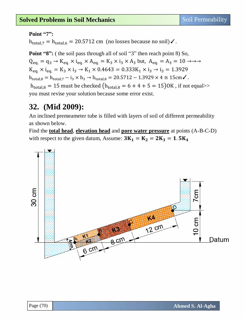
Page (70)
Soil Permeability Solved Problems in Soil Mechanics
Ahmed S. Al-Agha
Point “7”:
htotal,7 = htotal,6 = 20.5712 cm (no losses because no soil)✓.
Point “8”: ( the soil pass through all of soil “3” then reach point 8) So,
Qeq. = q3 → Keq. × ieq. × Aeq. = K3 × i3 × A3 but, Aeq. = A3 = 10 →→→
Keq. × ieq. = K3 × i3 → K1 × 0.4643 = 0.333K1 × i3 → i3 = 1.3929
htotal,8 = htotal,7 − i3 × h3 → htotal,8 = 20.5712 − 1.3929 × 4 ≅ 15cm✓.
htotal,8 = 15 must be checked (htotal,8 = 6 + 4 + 5 = 15)OK , if not equal>>
you must revise your solution because some error exist.
32. (Mid 2009): An inclined premeameter tube is filled with layers of soil of different permeability
as shown below.
Find the total head, elevation head and pore water pressure at points (A-B-C-D)
with respect to the given datum, Assume: 𝟑𝐊𝟏 = 𝐊𝟐 = 𝟐𝐊𝟑 = 𝟏. 𝟓𝐊𝟒
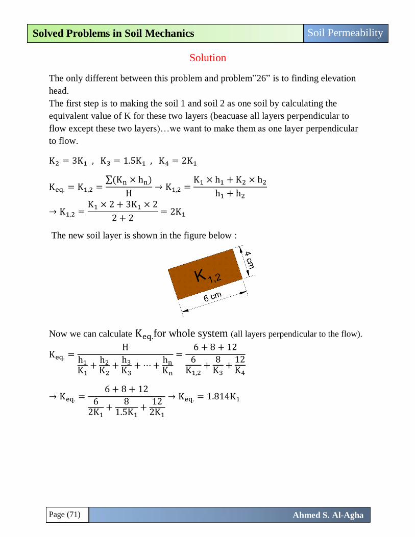
Page (71)
Soil Permeability Solved Problems in Soil Mechanics
Ahmed S. Al-Agha
Solution
The only different between this problem and problem”26” is to finding elevation
head.
The first step is to making the soil 1 and soil 2 as one soil by calculating the
equivalent value of K for these two layers (beacuase all layers perpendicular to
flow except these two layers)…we want to make them as one layer perpendicular
to flow.
K2 = 3K1 , K3 = 1.5K1 , K4 = 2K1
Keq. = K1,2 =∑(Kn × hn)
H→ K1,2 =
K1 × h1 + K2 × h2
h1 + h2
→ K1,2 =K1 × 2 + 3K1 × 2
2 + 2= 2K1
The new soil layer is shown in the figure below :
Now we can calculate Keq.for whole system (all layers perpendicular to the flow).
Keq. =H
h1K1
+h2K2
+h3
K3+ ⋯ +
hnKn
=6 + 8 + 12
6K1,2
+8
K3+
12K4
→ Keq. =6 + 8 + 12
62K1
+8
1.5K1+
122K1
→ Keq. = 1.814K1
Page (72)
Soil Permeability Solved Problems in Soil Mechanics
Ahmed S. Al-Agha
Firstly, we calculate the total head at each point.
∆Htotal = 30 − (10 + 7) = 13cm.
ieq. =∆Htotal
H=
13
6 + 8 + 12= 0.5
Qeq. = q1,2 = q3 = q4 , and Aeq. = 4 × 1 = A1,2 = A3 = A4 (Solution Key)
Point “A”:
htotal,A = 30cm(no losses because no soil) (Total head) ✓.
Point “B”: ( the soil pass through soil “1,2” then reach point B) So,
Qeq. = q1,2 → Keq. × ieq. × Aeq. = K1,2 × i1,2 × A1,2 but, Aeq. = A1,2 = 4 →→→
Keq. × ieq. = K1,2 × i1,2 → 1.814K1 × 0.5 = 2K1 × i1,2 → i1,2 = 0.4535
htotal,B = htotal,A − i1,2 × h1,2 → htotal,B = 30 − 0.4535 × 6 = 27.279cm✓.
Point “C”: (the soil pass through soil “3” then reach point C) So,
Qeq. = q3 → Keq. × ieq. × Aeq. = K3 × i3 × A3 but, Aeq. = A3 = 4 →→→
Keq. × ieq. = K3 × i3 → 1.814K1 × 0.5 = 1.5K1 × i3 → i3 = 0.6046
htotal,C = htotal,B − i3 × h3 → htotal,C = 27.279 − 0.6064 × 8 = 22.4278cm✓.
Point “D”: (the soil pass through soil “4” then reach point D) So,
Qeq. = q4 → Keq. × ieq. × Aeq. = K4 × i4 × A4 but, Aeq. = A4 = 4 →→→
Keq. × ieq. = K4 × i4 → 1.814K1 × 0.5 = 2K1 × i4 → i4 = 0.4535
htotal,D = htotal,C − i4 × h4 → htotal,D = 22.4278 − 0.4535 × 12 ≅ 17cm✓.
htotal,D = 17 must be checked (htotal,D = 10 + 7 = 17)OK , if not equal>> you
must revise your solution because some error exist.
Secondly, we calculate the elevation head at each point with respect to the given
datum.
By interpolation we calculate the elevation of each point from the datum as shown
in the following graph :
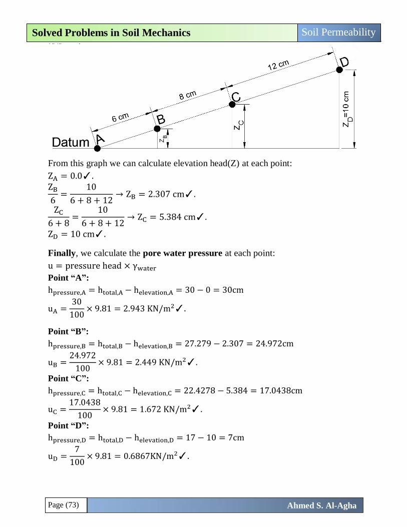
Page (73)
Soil Permeability Solved Problems in Soil Mechanics
Ahmed S. Al-Agha
From this graph we can calculate elevation head(Z) at each point:
ZA = 0.0✓. ZB
6=
10
6 + 8 + 12→ ZB = 2.307 cm✓.
ZC
6 + 8=
10
6 + 8 + 12→ ZC = 5.384 cm✓.
ZD = 10 cm✓.
Finally, we calculate the pore water pressure at each point:
u = pressure head × γwater
Point “A”:
hpressure,A = htotal,A − helevation,A = 30 − 0 = 30cm
uA =30
100× 9.81 = 2.943 KN/m2✓.
Point “B”:
hpressure,B = htotal,B − helevation,B = 27.279 − 2.307 = 24.972cm
uB =24.972
100× 9.81 = 2.449 KN/m2✓.
Point “C”:
hpressure,C = htotal,C − helevation,C = 22.4278 − 5.384 = 17.0438cm
uC =17.0438
100× 9.81 = 1.672 KN/m2✓.
Point “D”:
hpressure,D = htotal,D − helevation,D = 17 − 10 = 7cm
uD =7
100× 9.81 = 0.6867KN/m2✓.
Page (74)
Soil Permeability Solved Problems in Soil Mechanics
Ahmed S. Al-Agha
33. (Mid 2005): A pumping well test was made in sands extending to a depth of 15 m where
an impermeable stratum was encountered. The initial ground-water level was at the
ground surface. Observation wells were sited at distances of 3 and 7.5 m from the
pumping well. A steady state was established at about 20 hours when the discharge
was 3.8 L/s. The drawdowns at the two observation well were1.5 m and 0.35 m.
Calculate the coefficient of permeability.
K =q×loge(
r1r2
)
π×(h12−h2
2) K =
q×log10(r1r2
)
2.727×H×(h1−h2)
Solution
It’s clear that the problem about (un confined aquifer) you should know this
because there exist impermeable layer below sands and no any impermeable layer
above sand.
r1 = 7.5m(large value) , r2 = 3m(small value) , Htotal = 15 𝑚
d1 = 0.35m , d2 = 1.5m (drawdowns) يجب أن تكون القيمة الثانية أيضا d1هي الكبيرة وهي القيمة الثانية المعطاة في السؤال ..بالتالي قيمة r1نالحظ أن قيمة
h1 = Htotal − d1 = 15 − 0.35 = 14.65(large value)
h2 = Htotal − d2 = 15 − 1.5 = 13.5(small value)
Q = 3.8L
sec×
3600 sec
hr×
m3
1000L= 13.68m3/hr
Now, you are given two equations you must choose the coorect equation for un
confined aquifer (you must know the form of the equation of the two types)
K =q×loge(
r1r2
)
π×(h12−h2
2) note: loge (
r1
r2) =
Ln(r1r2
)
Ln(e)= Ln (
r1
r2) so the equation will be :
K =q × Ln (
r1
r2)
π × (h12 − h2
2)=
13.68 × Ln (7.53
)
π × (14.652 − 13.52)= 0.123m/hr✓.
Page (75)
Soil Permeability Solved Problems in Soil Mechanics
Ahmed S. Al-Agha
34.
A layer of sand 6 m thick lies beneath a clay stratum 5 m thick and above abed
thick shale( )نوع من الصخور . Inorder to determine the permeability of sand, a well
was driven to the top of the shale and water pumped out at a rate of 0.01m3/sec.
Two observation wells driven through the clay at 15m and 30 m from the pumping
well and water was found to rise to levels of 3m and 2.4 m below the ground water
surface. Calculate the permeability of soil.
Solution
It’s clear that the problem about (confined aquifer) because the clay layer
considered impermeable layer an shale is a type of rock , and the sand layer exist
between these two layers.
r1 = 30m(large value) , r2 = 15m(small value) , Htotal = 5 + 6 = 11 m
d1 = 2.4m , d2 = 3m [drawdowns, (below the ground water surface)]
h1 = Htotal − d1 = 11 − 2.4 = 8.6(large value)
h2 = Htotal − d2 = 11 − 3 = 8(small value)
Hsand = 6m
Q = 0.01m3/sec =36m3/hr
K =q × log10 (
r1
r2)
2.727 × H × (h1 − h2)=
36 × log10 (3015
)
2.727 × 6 × (8.6 − 8)= 1.1 m/hr✓.
Chapter (8)
Seepage
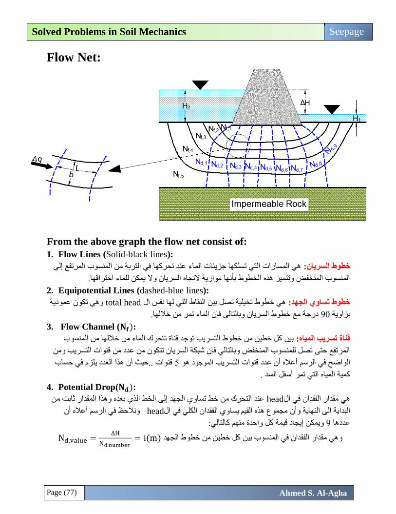
Page (77)
Seepage Solved Problems in Soil Mechanics
Ahmed S. Al-Agha
Flow Net:
From the above graph the flow net consist of:
1. Flow Lines (Solid-black lines):
ع إلى هي المسارات التي تسلكها جزيئات الماء عند تحركها في التربة من المنسوب المرتف خطوط السريان:
المنسوب المنخفض وتتميز هذه الخطوط بأنها موازية التجاه السريان وال يمكن للماء اختراقها.
2. Equipotential Lines (dashed-blue lines):
وهي تكون عمودية total headهي خطوط تخيلية تصل بين النقاط التي لها نفس ال خطوط تساوي الجهد:
ن الماء تمر من خاللها.إوبالتالي فدرجة مع خطوط السريان 90بزاوية
3. Flow Channel (𝐍𝐟):
بين كل خطين من خطوط التسريب توجد قناة تتحرك الماء من خاللها من المنسوب قناة تسريب المياه:
المرتفع حتى تصل للمنسوب المنخفض وبالتالي فإن شبكة السريان تتكون من عدد من قنوات التسريب ومن
قنوات ..حيث أن هذا العدد يلزم في حساب 5هو الموجودأعاله أن عدد قنوات التسريب الواضح في الرسم
كمية المياه التي تمر أسفل السد .
4. Potential Drop(𝐍𝐝):
عند التحرك من خط تساوي الجهد إلى الخط الذي بعده وهذا المقدار ثابت من headهي مقدار الفقدان في ال
ونالحظ في الرسم أعاله أن head مجموع هذه القيم يساوي الفقدان الكلي في ال البداية الى النهاية وأن
يجاد قيمة كل واحدة منهم كالتالي:إويمكن 9عددها
Nd,value =∆H
Nd,number = i(m) وهي مقدار الفقدان في المنسوب بين كل خطين من خطوط الجهد
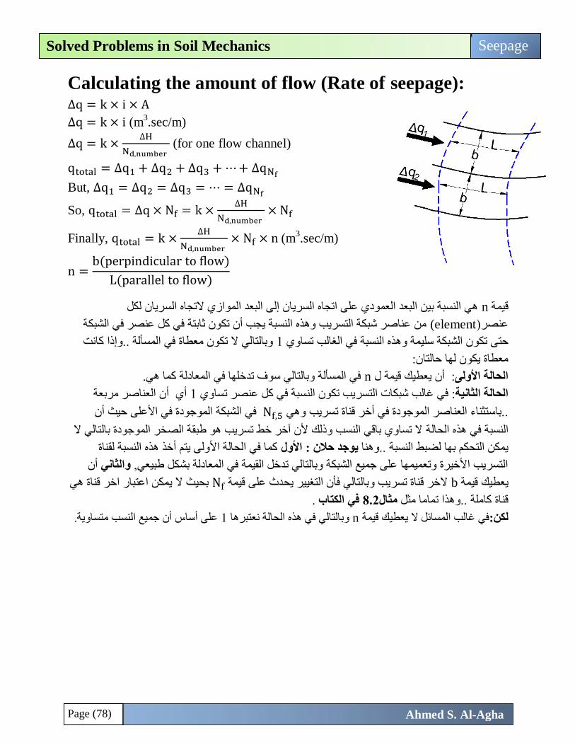
Page (78)
Seepage Solved Problems in Soil Mechanics
Ahmed S. Al-Agha
Calculating the amount of flow (Rate of seepage): ∆q = k × i × A
∆q = k × i (m3.sec/m)
∆q = k ×∆H
Nd,number (for one flow channel)
qtotal = ∆q1 + ∆q2 + ∆q3 + ⋯ + ∆qNf
But, ∆q1 = ∆q2 = ∆q3 = ⋯ = ∆qNf
So, qtotal = ∆q × Nf = k ×∆H
Nd,number × Nf
Finally, qtotal = k ×∆H
Nd,number × Nf × n (m3
.sec/m)
n =b(perpindicular to flow)
L(parallel to flow)
هي النسبة بين البعد العمودي على اتجاه السريان إلى البعد الموازي التجاه السريان لكل nقيمة
من عناصر شبكة التسريب وهذه النسبة يجب أن تكون ثابتة في كل عنصر في الشبكة element)عنصر)
ذا كانت إوبالتالي ال تكون معطاة في المسألة ..و 1ن الشبكة سليمة وهذه النسبة في الغالب تساوي حتى تكو
معطاة يكون لها حالتان:
في المسألة وبالتالي سوف تدخلها في المعادلة كما هي. n: أن يعطيك قيمة ل الحالة األولى
أي أن العناصر مربعة 1نصر تساوي : في غالب شبكات التسريب تكون النسبة في كل عالحالة الثانية
في الشبكة الموجودة في األعلى حيث أن Nf,5 ..باستثناء العناصر الموجودة في أخر قناة تسريب وهي
ال تساوي باقي النسب وذلك ألن آخر خط تسريب هو طبقة الصخر الموجودة بالتالي ال ةالنسبة في هذه الحال
كما في الحالة األولى يتم أخذ هذه النسبة لقناة األول : يوجد حالنهنا يمكن التحكم بها لضبط النسبة ..و
أن والثانيالتسريب األخيرة وتعميمها على جميع الشبكة وبالتالي تدخل القيمة في المعادلة بشكل طبيعي,
خر قناة هي بحيث ال يمكن اعتبار ا Nfالخر قناة تسريب وبالتالي فأن التغيير يحدث على قيمة bيعطيك قيمة
. في الكتاب 8.2مثالقناة كاملة ..وهذا تماما مثل
على أساس أن جميع النسب متساوية. 1وبالتالي في هذه الحالة نعتبرها nفي غالب المسائل ال يعطيك قيمة لكن:
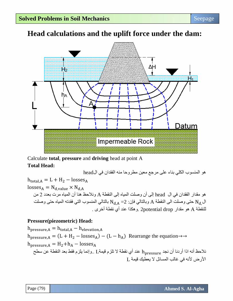
Page (79)
Seepage Solved Problems in Soil Mechanics
Ahmed S. Al-Agha
Head calculations and the uplift force under the dam:
Calculate total, pressure and driving head at point A
Total Head:
headهو المنسوب الكلي بناء على مرجع معين مطروحا منه الفقدان في ال
htotal,A = L + H2 − lossesA
lossesA = Nd,value × Nd,A
من 2ونالحظ هنا أن المياه مرت بعدد Aإلى أن وصلت المياه إلى النقطة headهو مقدار الفقدان في ال
بالتالي المنسوب التي فقدته المياه حتى وصلت Nd,A 2=وبالتالي فإن: Aحتى وصلت الى النقطة ,Ndال
.وهكذا عند أي نقطة أخرى . 2potential dropهو مقدار Aللنقطة
Pressure(piezometric) Head:
hpressure,A = htotal,A − helevation,A
hpressure,A = (L + H2 − lossesA) − (L − hA) Rearrange the equation→→
hpressure,A = H2+hA − lossesA
نما يلزم فقط بعد النقطة عن سطح إو.. Lعند أي نقطة ال تلزم قيمةhpressure ن نجد أردنا أنالحظ أنه اذا
Lاألرض ألنه في غالب المسائل ال يعطيك قيمة
Page (80)
Seepage Solved Problems in Soil Mechanics
Ahmed S. Al-Agha
Driving Head:
يسبب حركة وسريان الماء, أو بمعنى آخر هو الكمية المتبقية من ال يوط عند أي نقطة والذهو مقدار الهب
. H1لى المنسوب النهائيإ( عند أي نقطة والتي تسبب سريان الماء حتى تصل المياه H∆)الكلي headال
hDriving,A = ∆H − lossesA
Uplift force under the dam:
على أسفل السد والناتجة عن ضغط الماء الموجود أسفل السد)ك رد فعل لوزن ألعلى هي مقدار القوة المؤثرة
أسفل السد ولكن على شكل قوة لكل وحدة pore water pressureعن قيمة ال فهي تعبرالسد( وبالتالي
أول نقطة ذا كانت قاعدة السد)سطح التقاء السد مع التربة( مستوية ومنتظمة نجد الضغط عندإ يطول, وبالتال
وآخر نقطة أسفل السد ومن ثم نجد المساحة المتكونة من هذا الضغط. أما اذا لم تكن القاعدة مستوية ومنتظمة
فإننا نجد ضغط الماء عند كل تغير في شكل القاعدة ومن ثم نجد المساحة.
u = pressure head × γwater
uيجاد إعند تلك النقطة ومن ثم hpressureيجاد إوال أعند أي نقطة نريد ايجاد ضغط الماء عليها يجب
وسوف يتم حل مسائل بأفكار مختلفة لتوضيح الفكرة
Effective Stress at any point (chapter 9):
لكن في غالب األحيان يكون أحد المطاليب هو إيجاد 9هذا الموضوع سوف يتم تناوله بشكل مفصل في شبتر
: نقطة معينة وهو أمر بسيط كما يليقيمة االجهاد الفعال عند
اإلجهاد الفعال: هو الضغط الرأسي الناتج على نقطة معينة نتيجة وزن حبيبات التربة فقط )أي الحبيبات نفسها
بدون ماء(
At any point we can calculate the effective stress as following:
σtotal = σeffectiv + u → σeffectiv = σtotal − u
u = pore water pressure at any point (we calculate it as mentioned above)
σtotal = The total(vertical) stress applied on a point and can be calculated as following:
)إن وجدت(وأي أوزان أخرى هو الضغط الرأسي الكلي الناتج على نقطة معينة من وزن التربة ووزن الماء معا
For example at point A in the flow net on the last graph
σtotal,A = (H2 × γwater) + (hA × γsat)
وذلك ألنه متعلق باألوزان الموجودة فوق النقطة نفسها lossesنالحظ هنا ال يتم خصم أي
Now, we can calculate the effective stress easily.
σeffectiv = σtotal − u
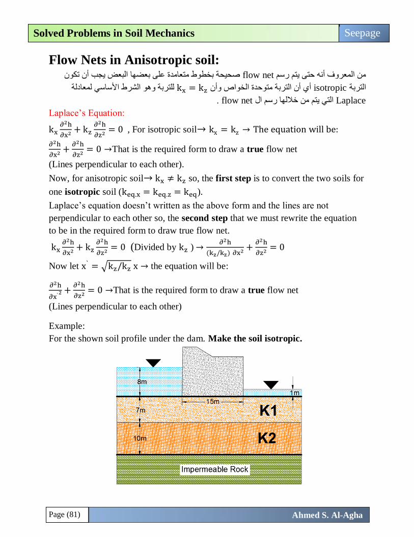
Page (81)
Seepage Solved Problems in Soil Mechanics
Ahmed S. Al-Agha
Flow Nets in Anisotropic soil: صحيحة بخطوط متعامدة على بعضها البعض يجب أن تكون flow netمن المعروف أنه حتى يتم رسم
kxأي أن التربة متوحدة الخواص وأن isotropicالتربة = kz للتربة وهو الشرط األساسي لمعادلة
Laplace ال التي يتم من خاللها رسمflow net .
Laplace’s Equation:
kx∂2h
∂x2+ kz
∂2h
∂z2= 0 , For isotropic soil→ kx = kz → The equation will be:
∂2h
∂x2+
∂2h
∂z2= 0 →That is the required form to draw a true flow net
(Lines perpendicular to each other).
Now, for anisotropic soil→ kx ≠ kz so, the first step is to convert the two soils for
one isotropic soil (keq.x = keq.z = keq).
Laplace’s equation doesn’t written as the above form and the lines are not
perpendicular to each other so, the second step that we must rewrite the equation
to be in the required form to draw true flow net.
kx∂2h
∂x2+ kz
∂2h
∂z2= 0 (Divided by kz ) →
∂2h
(kz/kz) ∂x2+
∂2h
∂z2= 0
Now let x` = √kz/kz x → the equation will be:
∂2h
∂x`2 +∂2h
∂z2= 0 →That is the required form to draw a true flow net
(Lines perpendicular to each other)
Example:
For the shown soil profile under the dam. Make the soil isotropic.
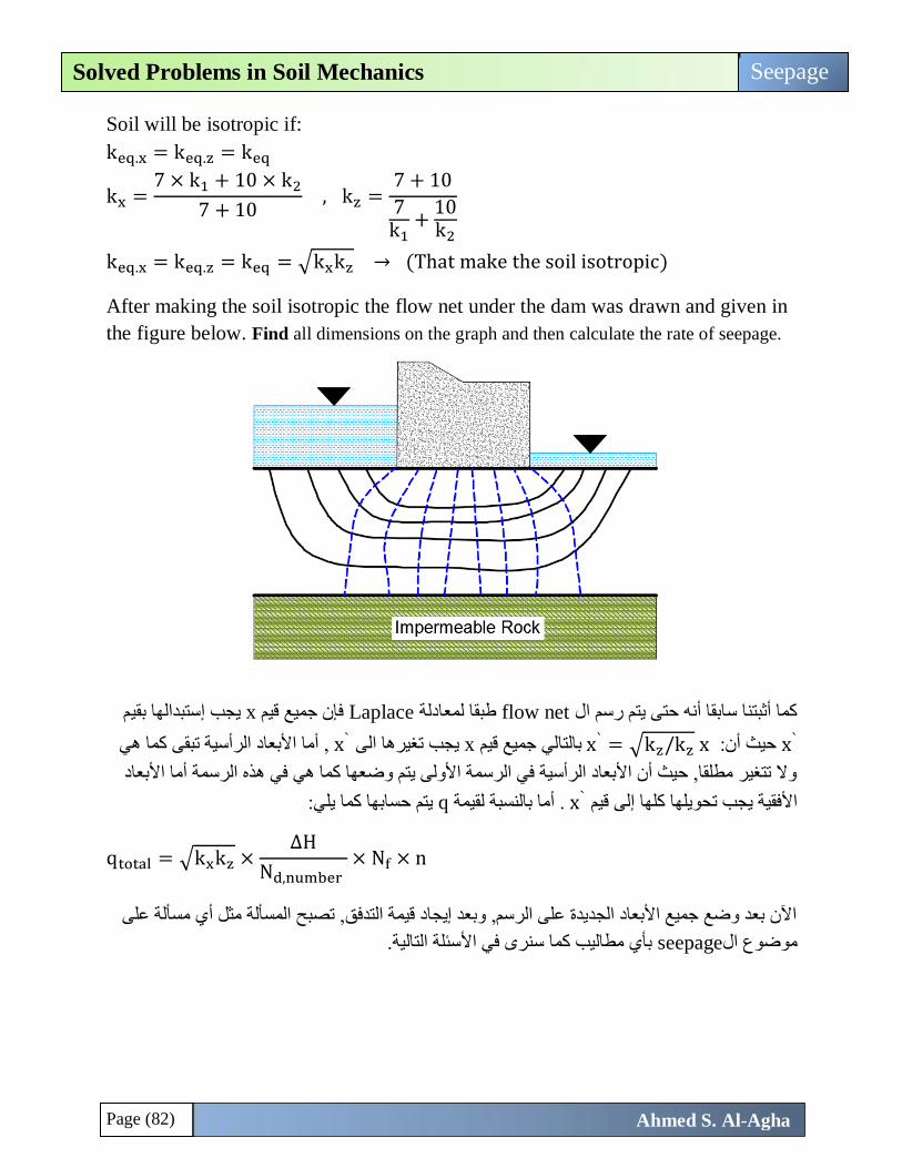
Page (82)
Seepage Solved Problems in Soil Mechanics
Ahmed S. Al-Agha
Soil will be isotropic if:
keq.x = keq.z = keq
kx =7 × k1 + 10 × k2
7 + 10 , kz =
7 + 10
7k1
+10k2
keq.x = keq.z = keq = √kxkz → (That make the soil isotropic)
After making the soil isotropic the flow net under the dam was drawn and given in
the figure below. Find all dimensions on the graph and then calculate the rate of seepage.
ستبدالها بقيمإيجب xفإن جميع قيم Laplaceطبقا لمعادلة flow netكما أثبتنا سابقا أنه حتى يتم رسم ال
x` :حيث أن x` = √kz/kz x بالتالي جميع قيمx يجب تغيرها الى x` أما األبعاد الرأسية تبقى كما هي ,
وال تتغير مطلقا, حيث أن األبعاد الرأسية في الرسمة األولى يتم وضعها كما هي في هذه الرسمة أما األبعاد
يتم حسابها كما يلي: qقيمة ل. أما بالنسبة `x لى قيم إاألفقية يجب تحويلها كلها
qtotal = √kxkz ×∆H
Nd,number × Nf × n
اآلن بعد وضع جميع األبعاد الجديدة على الرسم, وبعد إيجاد قيمة التدفق, تصبح المسألة مثل أي مسألة على
بأي مطاليب كما سنرى في األسئلة التالية. seepageموضوع ال
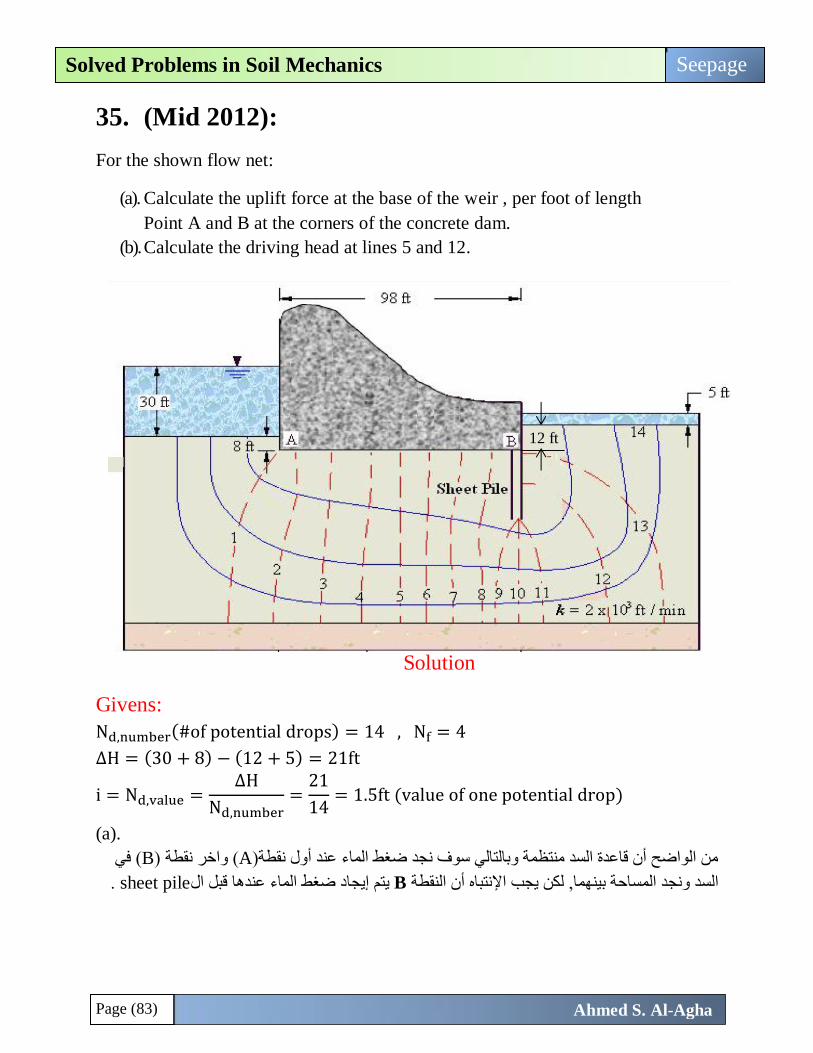
Page (83)
Seepage Solved Problems in Soil Mechanics
Ahmed S. Al-Agha
35. (Mid 2012):
For the shown flow net:
(a). Calculate the uplift force at the base of the weir , per foot of length
Point A and B at the corners of the concrete dam.
(b). Calculate the driving head at lines 5 and 12.
Solution
Givens:
Nd,number(#of potential drops) = 14 , Nf = 4
∆H = (30 + 8) − (12 + 5) = 21ft
i = Nd,value =∆H
Nd,number=
21
14= 1.5ft (value of one potential drop)
(a).
( في B( واخر نقطة )Aمن الواضح أن قاعدة السد منتظمة وبالتالي سوف نجد ضغط الماء عند أول نقطة)
. sheet pileإيجاد ضغط الماء عندها قبل اليتم Bنتباه أن النقطة إلالسد ونجد المساحة بينهما, لكن يجب ا
12 ft
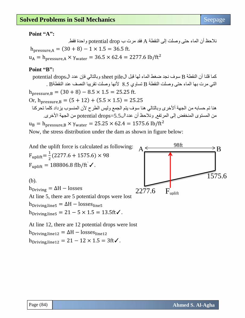
Page (84)
Seepage Solved Problems in Soil Mechanics
Ahmed S. Al-Agha
Point “A”:
واحدة فقط. potential dropفقد مرت ب Aنالحظ أن الماء حتى وصلت إلى النقطة
hpressure,A = (30 + 8) − 1 × 1.5 = 36.5 ft.
uA = hpressure,A × γwater = 36.5 × 62.4 = 2277.6 Ib/ft2
Point “B”:
potential dropsن عدد الإوبالتالي ف sheet pileوف نجد ضغط الماء لها قبل الس Bكما قلنا أن النقطة
. Bألنها وصلت تقريبا النصف عند النقطة 8.5تساوي Bالتي مرت بها الماء حتى وصلت النقطة
hpressure,B = (30 + 8) − 8.5 × 1.5 = 25.25 ft.
Or, hpressure,B = (5 + 12) + (5.5 × 1.5) = 25.25
الجهة أألخرى وبالتالي هنا سوف يتم الجمع وليس الطرح ألن المنسوب يزداد كلما تحركنا هنا تم حسابه من
من الجهة األخرى. potential drops=5.5الأن عدد ظمن المستوى المنخفض إلى المرتفع, ونالح
uB = hpressure,B × γwater = 25.25 × 62.4 = 1575.6 Ib/ft2
Now, the stress distribution under the dam as shown in figure below:
And the uplift force is calculated as following:
Fuplift=1
2(2277.6 + 1575.6) × 98
Fuplift = 188806.8 fIb/ft`✓.
(b).
hDriving = ∆H − losses
At line 5, there are 5 potential drops were lost
hDriving,line5 = ∆H − lossesline5
hDriving,line5 = 21 − 5 × 1.5 = 13.5ft✓.
At line 12, there are 12 potential drops were lost
hDriving,line12 = ∆H − lossesline12
hDriving,line12 = 21 − 12 × 1.5 = 3ft✓.
A B
2277.6
1575.6
Fuplift
98ft
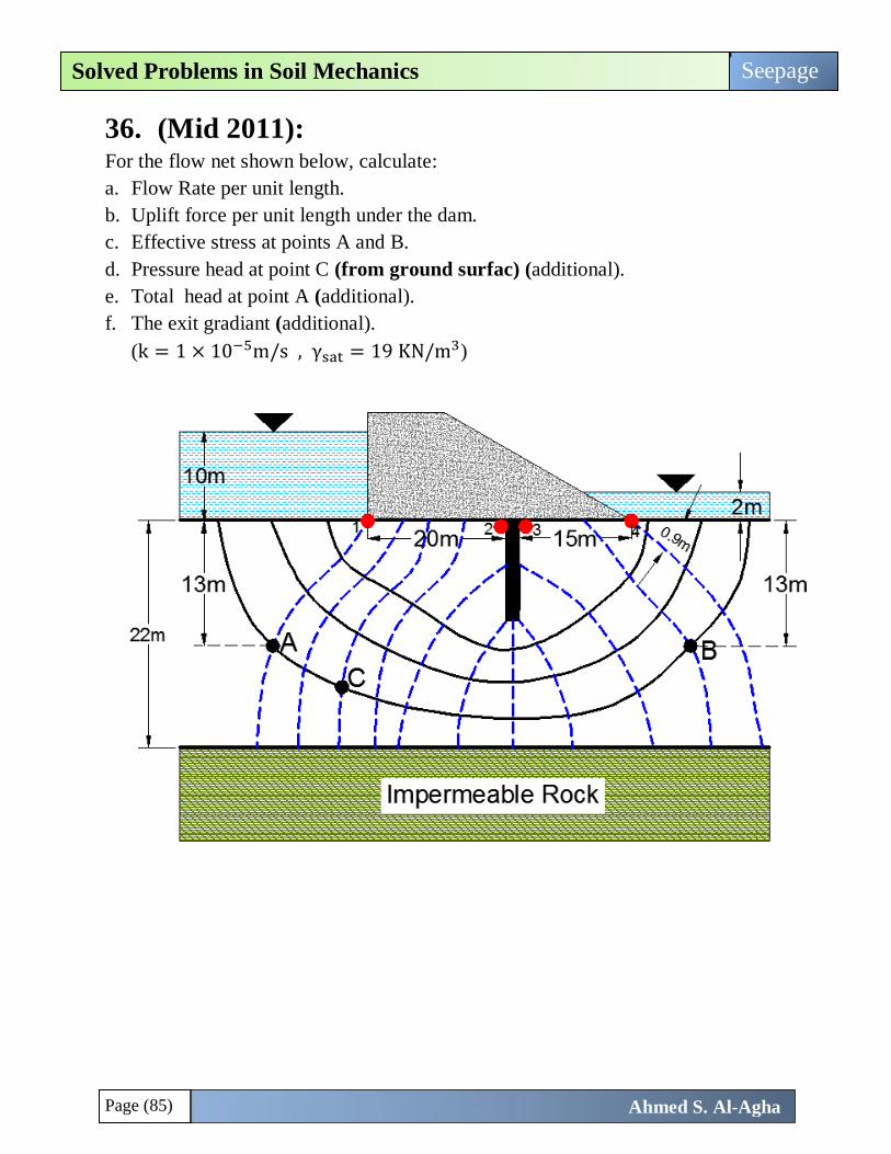
Page (85)
Seepage Solved Problems in Soil Mechanics
Ahmed S. Al-Agha
36. (Mid 2011): For the flow net shown below, calculate:
a. Flow Rate per unit length.
b. Uplift force per unit length under the dam.
c. Effective stress at points A and B.
d. Pressure head at point C (from ground surfac) (additional).
e. Total head at point A (additional).
f. The exit gradiant (additional).
(k = 1 × 10⁻⁵m/s , γsat = 19 KN/m3)
Page (86)
Seepage Solved Problems in Soil Mechanics
Ahmed S. Al-Agha
Solution
Givens:
Nd,number(#of potential drops) = 12 , Nf = 4 , k = 1 × 10⁻⁵m/s
∆H = (10) − (2) = 8 m , γsat = 19 KN/m3
i = Nd,value =∆H
Nd,number=
8
12= 0.667 m (value of one potential drop)
a.
q = k ×∆H
Nd,number × Nf × n = 1 × 10−5 × 0.667 × 4 × 1 = 2.668 × 10⁻⁵ m3/s.m✓.
b.
يجاد ضغط الماء عند كل تغير أسفل السد وبالتالي هنا يجب إيجادإإليجاد قوة ضغط الماء ألعلى يجب
ألنه وكما سنرى أنه sheet pileقطتين قبل وبعد النلى الإضافة الضغط عند أول نقطة وآخر نقطة باإل
يوجد فرق كبير بينهما.
Point “1”:
واحدة فقط. potential dropفقد مرت ب 1نالحظ أن الماء حتى وصلت إلى النقطة
hpressure,1 = 10 − 1 × 0.667 = 9.333m..
u1 = hpressure,1 × γwater = 9.333 × 9.81 = 91.55 KN/m2
Point “2”:
.5 وليس potential drop 4.5فقد مرت ب 2نالحظ أن الماء حتى وصلت إلى النقطة
hpressure,2 = 10 − 4.5 × 0.667 = 6.998m..
u2 = hpressure,2 × γwater = 6.998 × 9.81 = 68.65 KN/m2
Point “3”:
.10وليس 9.5potential dropفقد مرت ب 3نالحظ أن الماء حتى وصلت إلى النقطة
hpressure,3 = 10 − 9.5 × 0.667 = 3.663m..
u3 = hpressure,3 × γwater = 3.663 × 9.81 = 35.93KN/m2
Point “4”:
.potential drop 11فقد مرت ب 4نالحظ أن الماء حتى وصلت إلى النقطة
hpressure,4 = 10 − 11 × 0.667 = 2.663m..
u4 = hpressure,4 × γwater = 2.663 × 9.81 = 26.12KN/m2
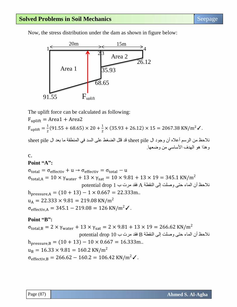
Page (87)
Seepage Solved Problems in Soil Mechanics
Ahmed S. Al-Agha
Now, the stress distribution under the dam as shown in figure below:
The uplift force can be calculated as following:
Fuplift = Area1 + Area2
Fuplift =1
2(91.55 + 68.65) × 20 +
1
2× (35.93 + 26.12) × 15 = 2067.38 KN/m2✓.
sheet pileما بعد ال قد قلل الضغط على السد في المنطقة sheet pileنالحظ من الرسم أعاله أن وجود ال
وهذا هو الهدف األساسي من وضعها.
c.
Point “A”:
σtotal = σeffectiv + u → σeffectiv = σtotal − u
σtotal,A = 10 × γwater + 13 × γsat = 10 × 9.81 + 13 × 19 = 345.1 KN/m2
potential drop 1فقد مرت ب Aنالحظ أن الماء حتى وصلت إلى النقطة
hpressure,A = (10 + 13) − 1 × 0.667 = 22.333m..
uA = 22.333 × 9.81 = 219.08 KN/m2
σeffectiv,A = 345.1 − 219.08 = 126 KN/m2✓.
Point “B”:
σtotal,B = 2 × γwater + 13 × γsat = 2 × 9.81 + 13 × 19 = 266.62 KN/m2
potential drop 10فقد مرت ب Bنالحظ أن الماء حتى وصلت إلى النقطة
hpressure,B = (10 + 13) − 10 × 0.667 = 16.333m..
uB = 16.33 × 9.81 = 160.2 KN/m2
σeffectiv,B = 266.62 − 160.2 = 106.42 KN/m2✓.
1 2 3
4
91.55
68.65
35.93
26.12
20m 15m
Fuplift
Area 1
Area 2
Page (88)
Seepage Solved Problems in Soil Mechanics
Ahmed S. Al-Agha
d.
لكن في كثير من األحيان ما يكون أحد hpressure,cنالحظ أن المعلومات غير كافية لحساب قيمة
معين ,مثال حدد في السؤال مستوى سطح المطاليب وبالتالي يجب إيجاد هذا الضغط بالنسبة لمرجع
األرض وقد ال يحدد مرجع أنت الذي تقرر.
وبالتالي: hcوسطح األرض )المرجع(هي Cاآلن نفرض أن المسافة بين النقطة
We note that, there are 3 potential drops to reach point C
hpressure,C = (10 + hc) − 3 × 0.667 = 7.99 + hc = 7.99(𝐚𝐛𝐨𝐯𝐞 𝐠𝐫𝐨𝐮𝐧𝐝 𝐬𝐮𝐫𝐟𝐚𝐜𝐞)
If the value 7.99 is negative value, that means (below the ground surface) ✓.
e.
htotal,A = (10 + 22) − lossesA → 1 potential drop to reach A
htotal,A = (10 + 22) − 0.667 × 1 = 31.333 m✓.
We note that, also we can calculate pressure head from total head
hpressure,A = htotal,A − helevation,A
hpressure,A = 31.333 − (22 − 13) = 22.333m (the same as calculated above).
f.
من الرسم أن يتضحموجودة في الشبكة و potential dropللمخرج أي آلخر iالمطلوب هنا هي قيمة
على مسافتها potential drop ذا قسمنا الفقدان في المنسوب في هذه الإ بالتالي 0.9مسافتها تساوي
للمخرج i فسنحصل على قيمة
iexit =exit losse
exit distance=
0.667
0.9= 0.741✓.
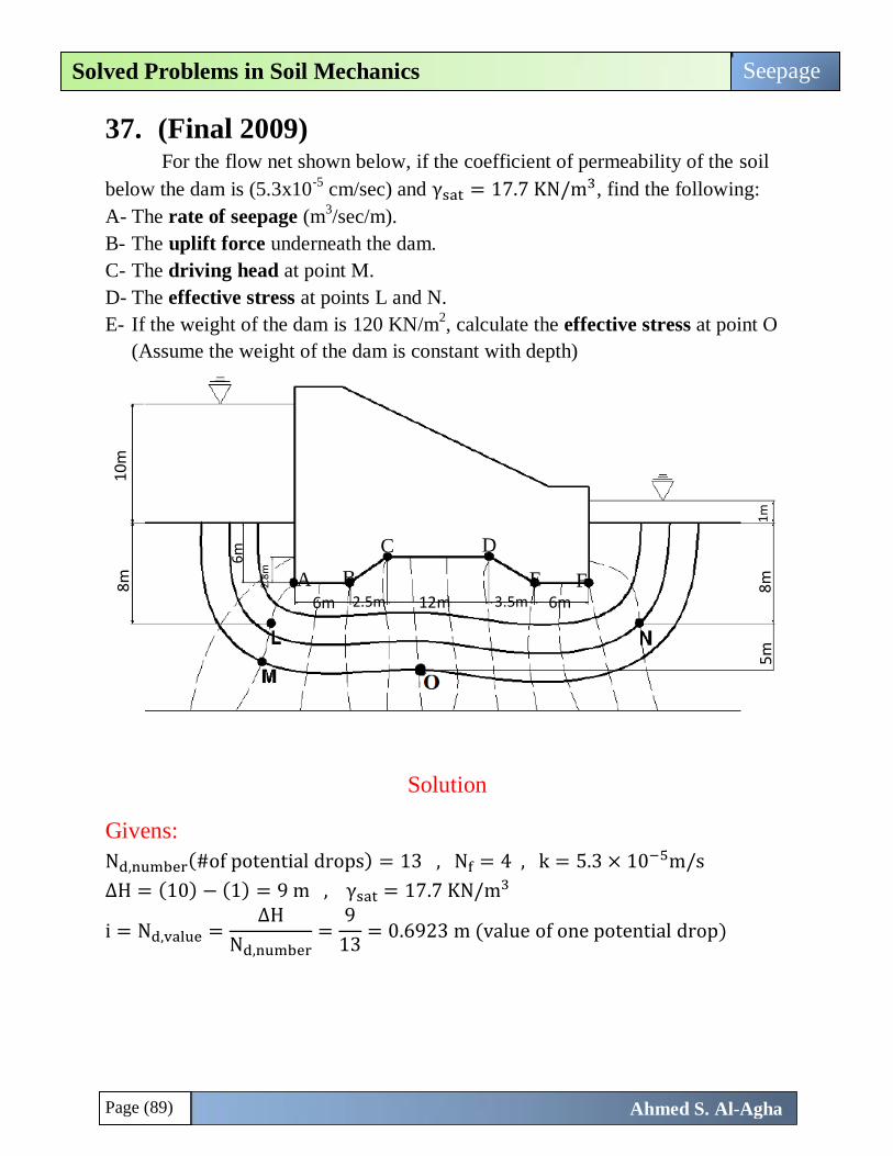
Page (89)
Seepage Solved Problems in Soil Mechanics
Ahmed S. Al-Agha
37. (Final 2009) For the flow net shown below, if the coefficient of permeability of the soil
below the dam is (5.3x10⁻⁵
cm/sec) and γsat = 17.7 KN/m3, find the following:
A- The rate of seepage (m3/sec/m).
B- The uplift force underneath the dam.
C- The driving head at point M.
D- The effective stress at points L and N.
E- If the weight of the dam is 120 KN/m2, calculate the effective stress at point O
(Assume the weight of the dam is constant with depth)
Solution
Givens:
Nd,number(#of potential drops) = 13 , Nf = 4 , k = 5.3 × 10⁻⁵m/s
∆H = (10) − (1) = 9 m , γsat = 17.7 KN/m3
i = Nd,value =∆H
Nd,number=
9
13= 0.6923 m (value of one potential drop)
5m
5m
10m
1m
8m
8m
6m 2.5m 12m 3.5m 6m
2.8
m 6m
A B
C D
E F
Page (90)
Seepage Solved Problems in Soil Mechanics
Ahmed S. Al-Agha
A-
q = k ×∆H
Nd,number × Nf × n = 5.3 × 10−5 × 0.6923 × 4 = 14.67 × 10⁻⁵ m3/s.m✓.
B-
A to F)نالحظ هنا أن قاعدة السد غير منتظمة وبالتالي يجب إيجاد ضغط الماء عند كل تغير)
Point “A”:
We note that, there are 2 potential drops to reach point A
hpressure,A = (10 + 6) − 2 × 0.6923 = 14.6154m.
uA = hpressure,A × γwater = 14.6154 × 9.81 = 143.377 KN/m2
Point “B”:
We note that, there are 4 potential drops to reach point B
hpressure,B = (10 + 6) − 4 × 0.6923 = 13.2308m.
uB = hpressure,B × γwater = 13.2308 × 9.81 = 129.794 KN/m2
Point “C”:
We note that, there are 5 potential drops to reach point C
hpressure,C = (10 + 6 − 2.8) − 5 × 0.6923 = 9.7385m.
uC = hpressure,C × γwater = 9.7385 × 9.81 = 95.534 KN/m2
Point “D”:
We note that, there are 8 potential drops to reach point D
hpressure,D = (10 + 6 − 2.8) − 8 × 0.6923 = 7.6616m.
uD = hpressure,D × γwater = 7.6616 × 9.81 = 75.16 KN/m2
Point “E”:
We note that, there are 9 potential drops to reach point E
hpressure,E = (10 + 6) − 9 × 0.6923 = 9.7693m.
uE = hpressure,E × γwater = 9.7693 × 9.81 = 95.836 KN/m2
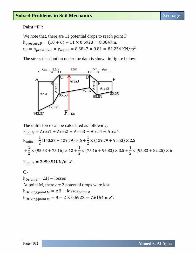
Page (91)
Seepage Solved Problems in Soil Mechanics
Ahmed S. Al-Agha
Point “F”:
We note that, there are 11 potential drops to reach point F
hpressure,F = (10 + 6) − 11 × 0.6923 = 8.3847m.
uF = hpressure,F × γwater = 8.3847 × 9.81 = 82.254 KN/m2
The stress distribution under the dam is shown in figure below:
The uplift force can be calculated as following:
Fuplift = Area1 + Area2 + Area3 + Area4 + Area4
Fuplift =1
2(143.37 + 129.79) × 6 +
1
2× (129.79 + 95.53) × 2.5
+1
2× (95.53 + 75.16) × 12 +
1
2× (75.16 + 95.83) × 3.5 +
1
2× (95.83 + 82.25) × 6
Fuplift = 2959.51KN/m`✓.
C-
hDriving = ∆H − losses
At point M, there are 2 potential drops were lost
hDriving,point M = ∆H − lossespoint M
hDriving,point M = 9 − 2 × 0.6923 = 7.6154 m✓.
A B
C D
E F
Area1
Area3
Area5
Are
a2
Are
a4
6m 2.5m 12m 3.5m 6m
143.37
129.79
95.53 75.16
95.83 82.25
Fuplift
Page (92)
Seepage Solved Problems in Soil Mechanics
Ahmed S. Al-Agha
D- Point “L”:
σtotal = σeffectiv + u → σeffectiv = σtotal − u
σtotal,L = 10 × γwater + 8 × γsat = 10 × 9.81 + 8 × 17.7 = 239.7 KN/m2
We note that, there are 2 potential drops to reach point L
hpressure,L = (10 + 8) − 2 × 0.6923 = 16.6154m.
uL = 16.6154 × 9.81 = 163 KN/m2
σeffectiv,L = 239.7 − 163 = 76.7 KN/m2✓.
Point “N”:
σtotal = σeffectiv + u → σeffectiv = σtotal − u
σtotal,N = 1 × γwater + 8 × γsat = 1 × 9.81 + 8 × 17.7 = 151.41 KN/m2
We note that, there are 12 potential drops to reach point N
hpressure,N = (10 + 8) − 12 × 0.6923 = 9.6924m.
uN = 9.6924 × 9.81 = 95.08 KN/m2
σeffectiv,N = 151.41 − 95.08 = 56.32 KN/m2✓.
E- (Additional)
جهادات الكلية عند هذه النقطة يجب أخذ كل إلتقع أسفل السد وبالتالي عند حساب ا Oنالحظ أن النقطة
جهادات الكلية عند هذه النقطة.إلاألوزان التي فوقها وبالتالي يجب إضافة وزن السد إلى ا
9.8m = (2.8+6-8+5) يساوي حتى الوصول إلى قاع السد Oنالحظ أيضا أن ارتفاع التربة فوق النقطة
Point “O”:
σtotal = σeffectiv + u → σeffectiv = σtotal − u
σtotal,O = 9.8 × γsat + dam weight = 9.8 × 17.7 + 120 = 293.46 KN/m2
We note that, there are 6 potential drops to reach point O
hpressure,O = (10 + 8 + 5) − 6 × 0.6923 = 18.846m.
uO = 18.846 × 9.81 = 184.88 KN/m2
σeffectiv,O = 293.46 − 184.88 = 108.578 KN/m2✓.
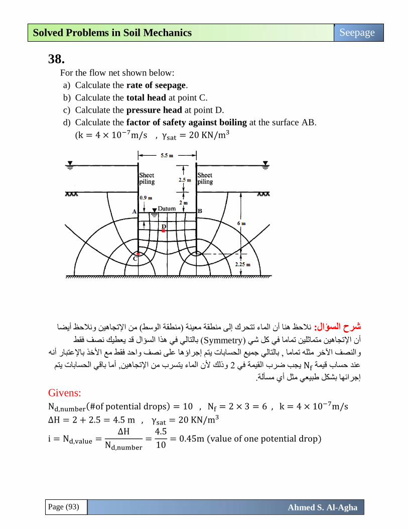
Page (93)
Seepage Solved Problems in Soil Mechanics
Ahmed S. Al-Agha
38.
For the flow net shown below:
a) Calculate the rate of seepage.
b) Calculate the total head at point C.
c) Calculate the pressure head at point D.
d) Calculate the factor of safety against boiling at the surface AB.
(k = 4 × 10⁻⁷m/s , γsat = 20 KN/m3
نالحظ هنا أن الماء تتحرك إلى منطقة معينة )منطقة الوسط( من اإلتجاهين ونالحظ أيضا شرح السؤال:
( بالتالي في هذا السؤال قد يعطيك نصف فقط Symmetryتجاهين متماثلين تماما في كل شي )إلأن ا
عتبار أنه إلالنصف اآلخر مثله تماما , بالتالي جميع الحسابات يتم إجراؤها على نصف واحد فقط مع األخذ باو
وذلك ألن الماء يتسرب من اإلتجاهين, أما باقي الحسابات يتم 2 يجب ضرب القيمة في Nfقيمة عند حساب
.إجرائها بشكل طبيعي مثل أي مسألة
Givens:
Nd,number(#of potential drops) = 10 , Nf = 2 × 3 = 6 , k = 4 × 10⁻⁷m/s
∆H = 2 + 2.5 = 4.5 m , γsat = 20 KN/m3
i = Nd,value =∆H
Nd,number=
4.5
10= 0.45m (value of one potential drop)
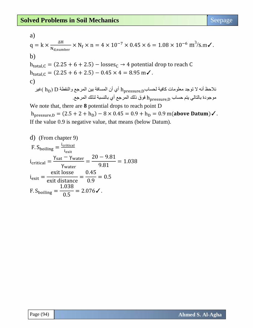
Page (94)
Seepage Solved Problems in Soil Mechanics
Ahmed S. Al-Agha
a)
q = k ×∆H
Nd,number × Nf × n = 4 × 10−7 × 0.45 × 6 = 1.08 × 10⁻⁶ m
3/s.m✓.
b)
htotal,C = (2.25 + 6 + 2.5) − lossesC → 4 potential drop to reach C
htotal,C = (2.25 + 6 + 2.5) − 0.45 × 4 = 8.95 m✓.
c)
غير D (hD )أي أن المسافة بين المرجع والنقطة hpressure,Dنالحظ أنه ال توجد معلومات كافية لحساب
جع أي بالنسبة لذلك المرجع.فوق ذلك المر hpressure,Dموجودة بالتالي يتم حساب
We note that, there are 8 potential drops to reach point D
hpressure,D = (2.5 + 2 + hD) − 8 × 0.45 = 0.9 + hD = 0.9 m(𝐚𝐛𝐨𝐯𝐞 𝐃𝐚𝐭𝐮𝐦)✓.
If the value 0.9 is negative value, that means (below Datum).
d) (From chapter 9)
F. Sboiling =icritical
iexit
icritical =γsat − γwater
γwater=
20 − 9.81
9.81= 1.038
iexit =exit losse
exit distance=
0.45
0.9= 0.5
F. Sboiling =1.038
0.5= 2.076✓.
Chapter (9)
In Situ Stresses
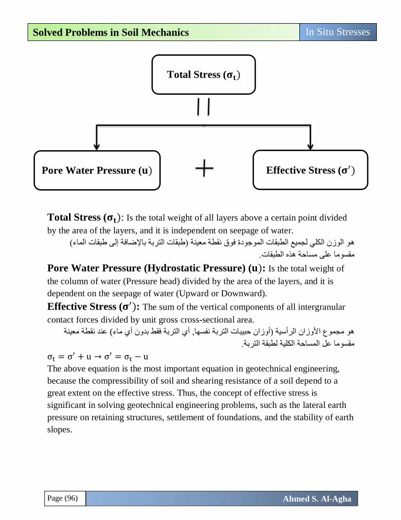
Page (96)
In Situ Stresses Solved Problems in Soil Mechanics
Ahmed S. Al-Agha
Total Stress (𝛔𝐭)
Pore Water Pressure (𝐮)
Effective Stress (𝛔′)
Total Stress (𝛔𝐭): Is the total weight of all layers above a certain point divided
by the area of the layers, and it is independent on seepage of water.
و الوزن الكلي لجميع الطبقات الموجودة فوق نقطة معينة )طبقات التربة باإلضافة إلى طبقات الماء( ه
مقسوما على مساحة هذه الطبقات.
Pore Water Pressure (Hydrostatic Pressure) (𝐮): Is the total weight of
the column of water (Pressure head) divided by the area of the layers, and it is
dependent on the seepage of water (Upward or Downward).
Effective Stress (𝛔′): The sum of the vertical components of all intergranular
contact forces divided by unit gross cross-sectional area.
عند نقطة معينة )أي التربة فقط بدون أي ماء نفسها,هو مجموع األوزان الرأسية )أوزان حبيبات التربة
مقسوما عل المساحة الكلية لطبقة التربة.
σt = σ′ + u → σ′ = σt − u
The above equation is the most important equation in geotechnical engineering,
because the compressibility of soil and shearing resistance of a soil depend to a
great extent on the effective stress. Thus, the concept of effective stress is
significant in solving geotechnical engineering problems, such as the lateral earth
pressure on retaining structures, settlement of foundations, and the stability of earth
slopes.
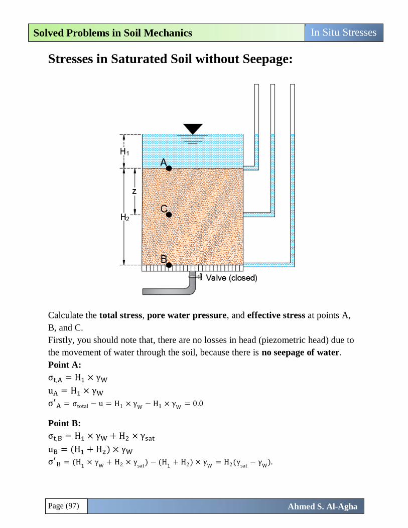
Page (97)
In Situ Stresses Solved Problems in Soil Mechanics
Ahmed S. Al-Agha
Stresses in Saturated Soil without Seepage:
Calculate the total stress, pore water pressure, and effective stress at points A,
B, and C.
Firstly, you should note that, there are no losses in head (piezometric head) due to
the movement of water through the soil, because there is no seepage of water.
Point A:
σt,A = H1 × γW
uA = H1 × γW
σ′A = σtotal − u = H1 × γ
W− H1 × γ
W= 0.0
Point B:
σt,B = H1 × γW + H2 × γsat
uB = (H1 + H2) × γW
σ′B = (H
1× γ
W+ H2 × γ
sat) − (H
1+ H2) × γ
W= H2(γ
sat− γ
W).
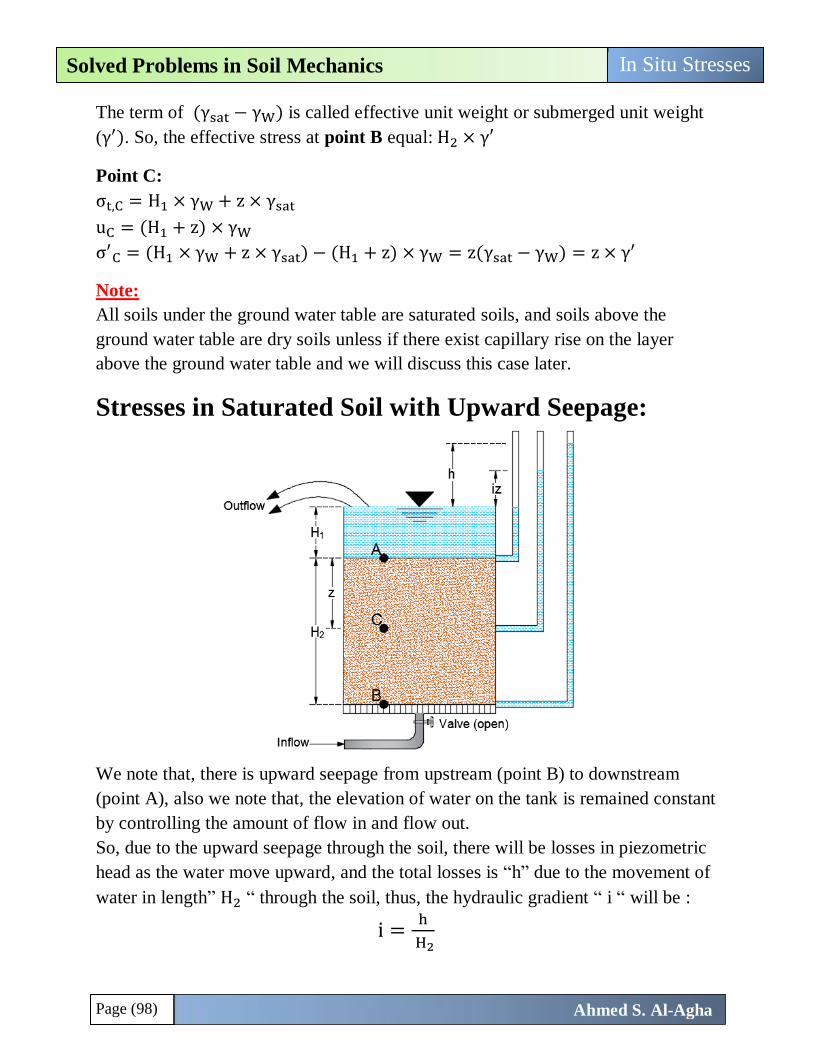
Page (98)
In Situ Stresses Solved Problems in Soil Mechanics
Ahmed S. Al-Agha
The term of (γsat − γW) is called effective unit weight or submerged unit weight
(γ′). So, the effective stress at point B equal: H2 × γ′
Point C:
σt,C = H1 × γW + z × γsat
uC = (H1 + z) × γW
σ′C = (H1 × γW + z × γsat) − (H1 + z) × γW = z(γsat − γW) = z × γ′
Note:
All soils under the ground water table are saturated soils, and soils above the
ground water table are dry soils unless if there exist capillary rise on the layer
above the ground water table and we will discuss this case later.
Stresses in Saturated Soil with Upward Seepage:
We note that, there is upward seepage from upstream (point B) to downstream
(point A), also we note that, the elevation of water on the tank is remained constant
by controlling the amount of flow in and flow out.
So, due to the upward seepage through the soil, there will be losses in piezometric
head as the water move upward, and the total losses is “h” due to the movement of
water in length” H2 “ through the soil, thus, the hydraulic gradient “ i “ will be :
i =h
H2
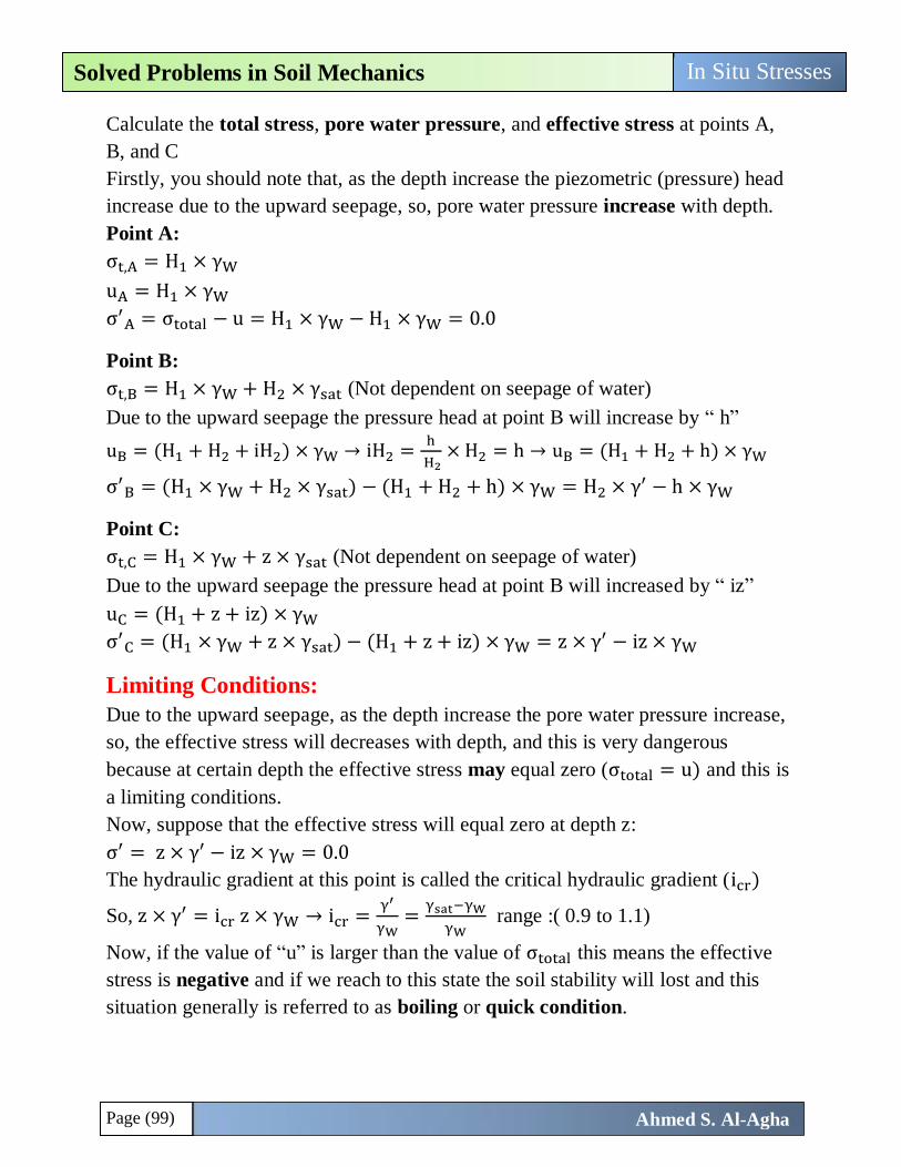
Page (99)
In Situ Stresses Solved Problems in Soil Mechanics
Ahmed S. Al-Agha
Calculate the total stress, pore water pressure, and effective stress at points A,
B, and C
Firstly, you should note that, as the depth increase the piezometric (pressure) head
increase due to the upward seepage, so, pore water pressure increase with depth.
Point A:
σt,A = H1 × γW
uA = H1 × γW
σ′A = σtotal − u = H1 × γW − H1 × γW = 0.0
Point B:
σt,B = H1 × γW + H2 × γsat (Not dependent on seepage of water)
Due to the upward seepage the pressure head at point B will increase by “ h”
uB = (H1 + H2 + iH2) × γW → iH2 =h
H2× H2 = h → uB = (H1 + H2 + h) × γW
σ′B = (H1 × γW + H2 × γsat) − (H1 + H2 + h) × γW = H2 × γ′ − h × γW
Point C:
σt,C = H1 × γW + z × γsat (Not dependent on seepage of water)
Due to the upward seepage the pressure head at point B will increased by “ iz”
uC = (H1 + z + iz) × γW
σ′C = (H1 × γW + z × γsat) − (H1 + z + iz) × γW = z × γ′ − iz × γW
Limiting Conditions:
Due to the upward seepage, as the depth increase the pore water pressure increase,
so, the effective stress will decreases with depth, and this is very dangerous
because at certain depth the effective stress may equal zero (σtotal = u) and this is
a limiting conditions.
Now, suppose that the effective stress will equal zero at depth z:
σ′ = z × γ′ − iz × γW = 0.0
The hydraulic gradient at this point is called the critical hydraulic gradient (icr)
So, z × γ′ = icr z × γW → icr =γ′
γW=
γsat−γW
γW range :( 0.9 to 1.1)
Now, if the value of “u” is larger than the value of σtotal this means the effective
stress is negative and if we reach to this state the soil stability will lost and this
situation generally is referred to as boiling or quick condition.
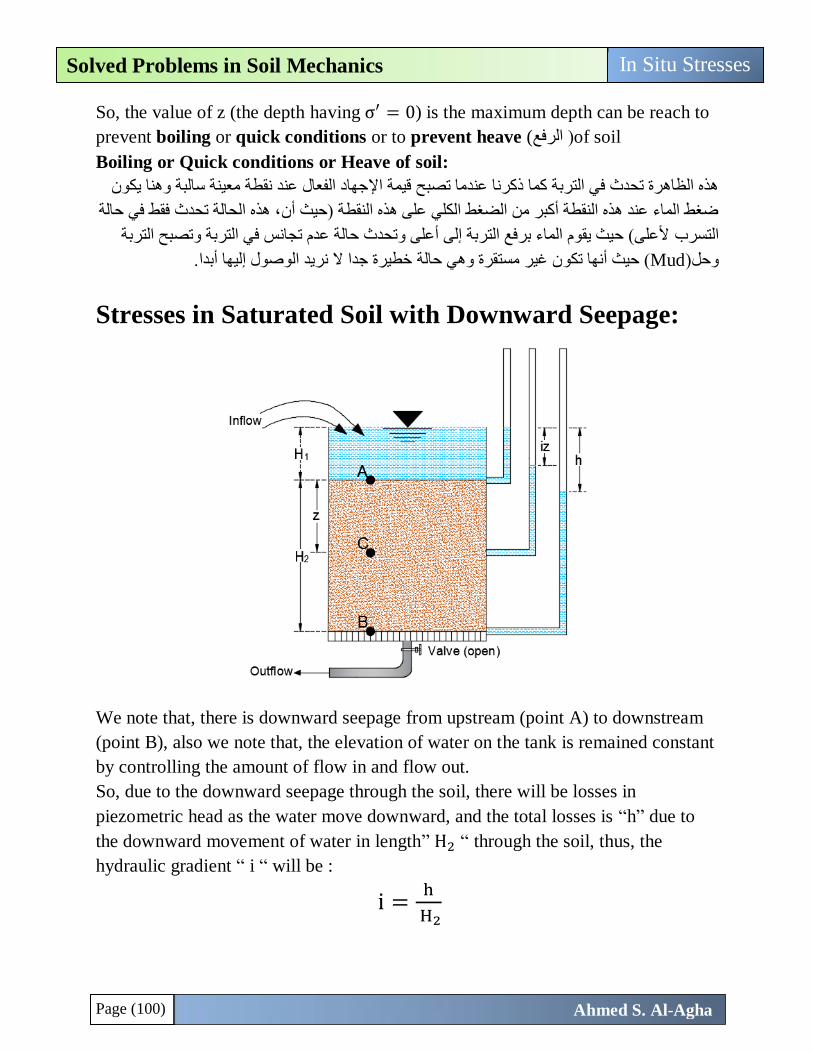
Page (100)
In Situ Stresses Solved Problems in Soil Mechanics
Ahmed S. Al-Agha
So, the value of z (the depth having σ′ = 0) is the maximum depth can be reach to
prevent boiling or quick conditions or to prevent heave (الرفع (of soil
Boiling or Quick conditions or Heave of soil:
جهاد الفعال عند نقطة معينة سالبة وهنا يكون هذه الظاهرة تحدث في التربة كما ذكرنا عندما تصبح قيمة اإل
، هذه الحالة تحدث فقط في حالة نضغط الماء عند هذه النقطة أكبر من الضغط الكلي على هذه النقطة )حيث أ
ألعلى( حيث يقوم الماء برفع التربة إلى أعلى وتحدث حالة عدم تجانس في التربة وتصبح التربة التسرب
ن غير مستقرة وهي حالة خطيرة جدا ال نريد الوصول إليها أبدا.( حيث أنها تكوMudوحل)
Stresses in Saturated Soil with Downward Seepage:
We note that, there is downward seepage from upstream (point A) to downstream
(point B), also we note that, the elevation of water on the tank is remained constant
by controlling the amount of flow in and flow out.
So, due to the downward seepage through the soil, there will be losses in
piezometric head as the water move downward, and the total losses is “h” due to
the downward movement of water in length” H2 “ through the soil, thus, the
hydraulic gradient “ i “ will be :
i =h
H2
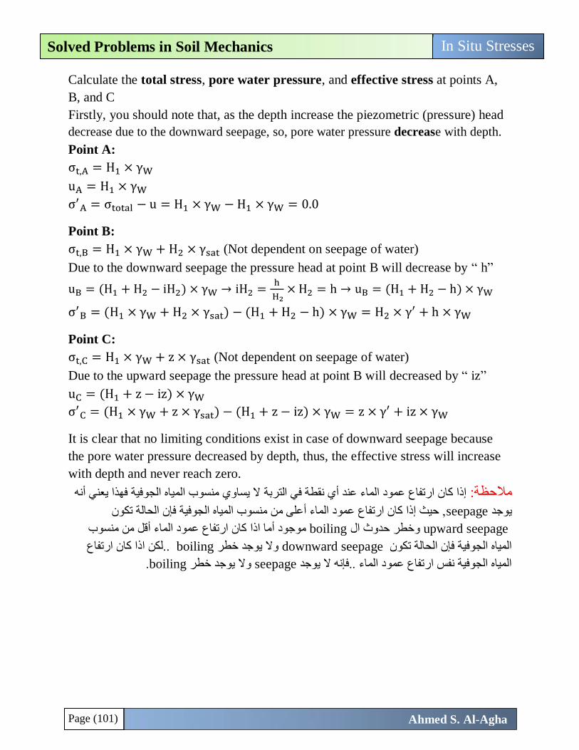
Page (101)
In Situ Stresses Solved Problems in Soil Mechanics
Ahmed S. Al-Agha
Calculate the total stress, pore water pressure, and effective stress at points A,
B, and C
Firstly, you should note that, as the depth increase the piezometric (pressure) head
decrease due to the downward seepage, so, pore water pressure decrease with depth.
Point A:
σt,A = H1 × γW
uA = H1 × γW
σ′A = σtotal − u = H1 × γW − H1 × γW = 0.0
Point B:
σt,B = H1 × γW + H2 × γsat (Not dependent on seepage of water)
Due to the downward seepage the pressure head at point B will decrease by “ h”
uB = (H1 + H2 − iH2) × γW → iH2 =h
H2× H2 = h → uB = (H1 + H2 − h) × γW
σ′B = (H1 × γW + H2 × γsat) − (H1 + H2 − h) × γW = H2 × γ′ + h × γW
Point C:
σt,C = H1 × γW + z × γsat (Not dependent on seepage of water)
Due to the upward seepage the pressure head at point B will decreased by “ iz”
uC = (H1 + z − iz) × γW
σ′C = (H1 × γW + z × γsat) − (H1 + z − iz) × γW = z × γ′ + iz × γW
It is clear that no limiting conditions exist in case of downward seepage because
the pore water pressure decreased by depth, thus, the effective stress will increase
with depth and never reach zero.
ال يساوي منسوب المياه الجوفية فهذا يعني أنه إذا كان ارتفاع عمود الماء عند أي نقطة في التربة مالحظة:
, حيث إذا كان ارتفاع عمود الماء أعلى من منسوب المياه الجوفية فإن الحالة تكونseepageيوجد
upward seepage وخطر حدوث الboiling كان ارتفاع عمود الماء أقل من منسوب موجود أما اذا
..لكن اذا كان ارتفاع boilingوال يوجد خطر downward seepageالمياه الجوفية فإن الحالة تكون
.boilingوال يوجد خطر seepageالمياه الجوفية نفس ارتفاع عمود الماء ..فإنه ال يوجد
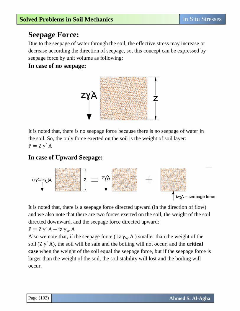
Page (102)
In Situ Stresses Solved Problems in Soil Mechanics
Ahmed S. Al-Agha
Seepage Force: Due to the seepage of water through the soil, the effective stress may increase or
decrease according the direction of seepage, so, this concept can be expressed by
seepage force by unit volume as following:
In case of no seepage:
It is noted that, there is no seepage force because there is no seepage of water in
the soil. So, the only force exerted on the soil is the weight of soil layer:
P = Z γ′ A
In case of Upward Seepage:
It is noted that, there is a seepage force directed upward (in the direction of flow)
and we also note that there are two forces exerted on the soil, the weight of the soil
directed downward, and the seepage force directed upward:
P = Z γ′ A − iz γw A
Also we note that, if the seepage force ( iz γw A ) smaller than the weight of the
soil (Z γ′ A), the soil will be safe and the boiling will not occur, and the critical
case when the weight of the soil equal the seepage force, but if the seepage force is
larger than the weight of the soil, the soil stability will lost and the boiling will
occur.
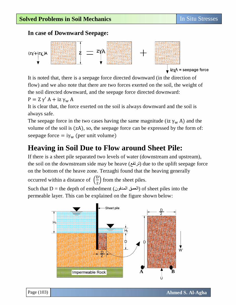
Page (103)
In Situ Stresses Solved Problems in Soil Mechanics
Ahmed S. Al-Agha
In case of Downward Seepage:
It is noted that, there is a seepage force directed downward (in the direction of
flow) and we also note that there are two forces exerted on the soil, the weight of
the soil directed downward, and the seepage force directed downward:
P = Z γ′ A + iz γw A
It is clear that, the force exerted on the soil is always downward and the soil is
always safe.
The seepage force in the two cases having the same magnitude (iz γw A) and the
volume of the soil is (zA), so, the seepage force can be expressed by the form of:
seepage force = iγw (per unit volume)
Heaving in Soil Due to Flow around Sheet Pile: If there is a sheet pile separated two levels of water (downstream and upstream),
the soil on the downstream side may be heave (ترتفع) due to the uplift seepage force
on the bottom of the heave zone. Terzaghi found that the heaving generally
occurred within a distance of (D
2) from the sheet piles.
Such that D = the depth of embedment (العمق المدفون) of sheet piles into the
permeable layer. This can be explained on the figure shown below:
A B
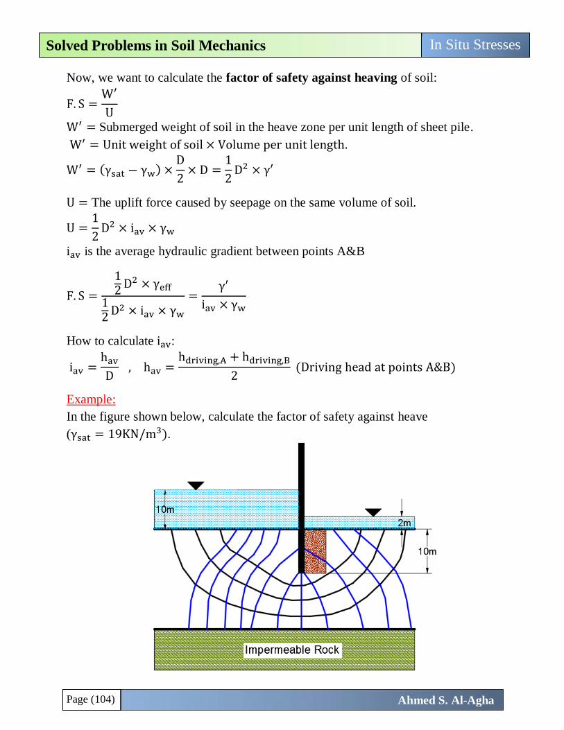
Page (104)
In Situ Stresses Solved Problems in Soil Mechanics
Ahmed S. Al-Agha
Now, we want to calculate the factor of safety against heaving of soil:
F. S =W′
U
W′ = Submerged weight of soil in the heave zone per unit length of sheet pile.
W′ = Unit weight of soil × Volume per unit length.
W′ = (γsat − γw) ×D
2× D =
1
2D2 × γ′
U = The uplift force caused by seepage on the same volume of soil.
U =1
2D2 × iav × γw
iav is the average hydraulic gradient between points A&B
F. S =
12
D2 × γeff
12
D2 × iav × γw
=γ′
iav × γw
How to calculate iav:
iav =hav
D , hav =
hdriving,A + hdriving,B
2 (Driving head at points A&B)
Example:
In the figure shown below, calculate the factor of safety against heave
(γsat = 19KN/m3).
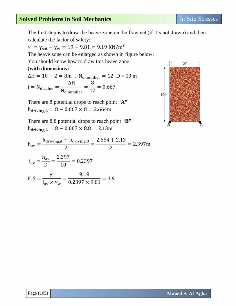
Page (105)
In Situ Stresses Solved Problems in Soil Mechanics
Ahmed S. Al-Agha
The first step is to draw the heave zone on the flow net (if it’s not drawn) and then
calculate the factor of safety:
γ′ = γsat − γw = 19 − 9.81 = 9.19 KN/m3
The heave zone can be enlarged as shown in figure below:
You should know how to draw this heave zone
(with dimensions)
∆H = 10 − 2 = 8m , Nd,number = 12 D = 10 m
i = Nd,value =∆H
Nd,number=
8
12= 0.667
There are 8 potential drops to reach point “A”
hdriving,A = 8 − 0.667 × 8 = 2.664m
There are 8.8 potential drops to reach point “B”
hdriving,A = 8 − 0.667 × 8.8 = 2.13m
hav =hdriving,A + hdriving,B
2=
2.664 + 2.13
2= 2.397m
iav =hav
D=
2.397
10= 0.2397
F. S =γ′
iav × γw=
9.19
0.2397 × 9.81= 3.9
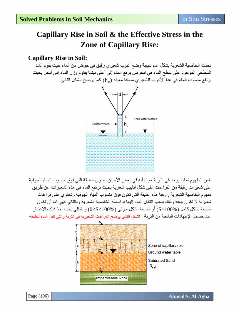
Page (106)
In Situ Stresses Solved Problems in Soil Mechanics
Ahmed S. Al-Agha
Capillary Rise in Soil & the Effective Stress in the
Zone of Capillary Rise:
Capillary Rise in Soil:
تحدث الخاصية الشعرية بشكل عام نتيجة وضع أنبوب شعيري رقيق في حوض من الماء حيث يقوم الشد
ى أعلى بينما يقاوم وزن الماء إلى أسفل بحيث السطحي الموجود على سطح الماء في الحوض برفع الماء إل
كما يوضح الشكل التالي: (hc)ا األنبوب الشعيري مسافة معينة يرتفع منسوب الماء في هذ
نفس المفهوم تماما يوجد في التربة حيث أنه في بعض األحيان تحتوي الطبقة التي فوق منسوب المياه الجوفية
ريق رية بحيث ترتفع الماء في هذه الشعيرات عن طعلى شعيرات رقيقة من الفراغات على شكل أنابيب شع
مفهوم الخاصية الشعرية , وهنا هذه الطبقة التي تكون فوق منسوب المياه الجوفية وتحتوي على فراغات
وبالتالي فهي اما أن تكون الماء إليها بواسطة الخاصية الشعرية انتقالرية ال تكون جافة وذلك بسبب يشع
يجب أخذ ذلك باالعتبار ي ( وبالتالS<100%>0( أو مشبعة بشكل جزئي )S=100%مشبعة بشكل كامل )
رية في التربة والتي تنقل الماء للطبقة:يالشكل التالي يوضح الفراغات الشع . عند حساب اإلجهادات الناتجة من التربة
Page (107)
In Situ Stresses Solved Problems in Soil Mechanics
Ahmed S. Al-Agha
To calculate total stress result from zone of capillary rise you should calculate the
unit weight of this layer [saturated or moist (partially saturated)] and then multiply
this unit weight by the height of this layer.
To calculate the pore water pressure from the zone of capillary rise:
u = − (S
100) γwh
S = Degree of saturation (%)
h = The height of the point under consideration measured from the groundwater
…....table.
Now, to find the pore water pressure at point B on the above graph you must
calculate it just before point (B) and just after point (B), because the degree of
saturation(S) is different before and after point (B)
So, to find effective stress at point (B) you must calculate it just before and just
after point (B).
The negative sign in the equation is due to the points always exist above the G.W.T.
بالنسبة لضغط الماء ...دائما أي نقطة توجد على نفس منسوب المياه الجوفية يكون ضغط الماء مالحظة:
عد هذه النقطة عن عندها صفر, وأي نقطة تكون أسفل منسوب المياه الجوفية يكون ضغط الماء لها مساويا ب
ة فوق منسوب المياه الجوفية يكون كثافة الماء النوعية, واذا كانت النقطمنسوب المياه الجوفية مضروبا في
ضغط الماء لها يساوي صفر إال إذا كانت هذه النقطة موجودة في طبقة حدثت فيها الخاصية الشعرية بحيث
يكون لهذه النقطة ضغط ماء ولكن ضغط سالب ألنها فوق منسوب المياه الجوفية.
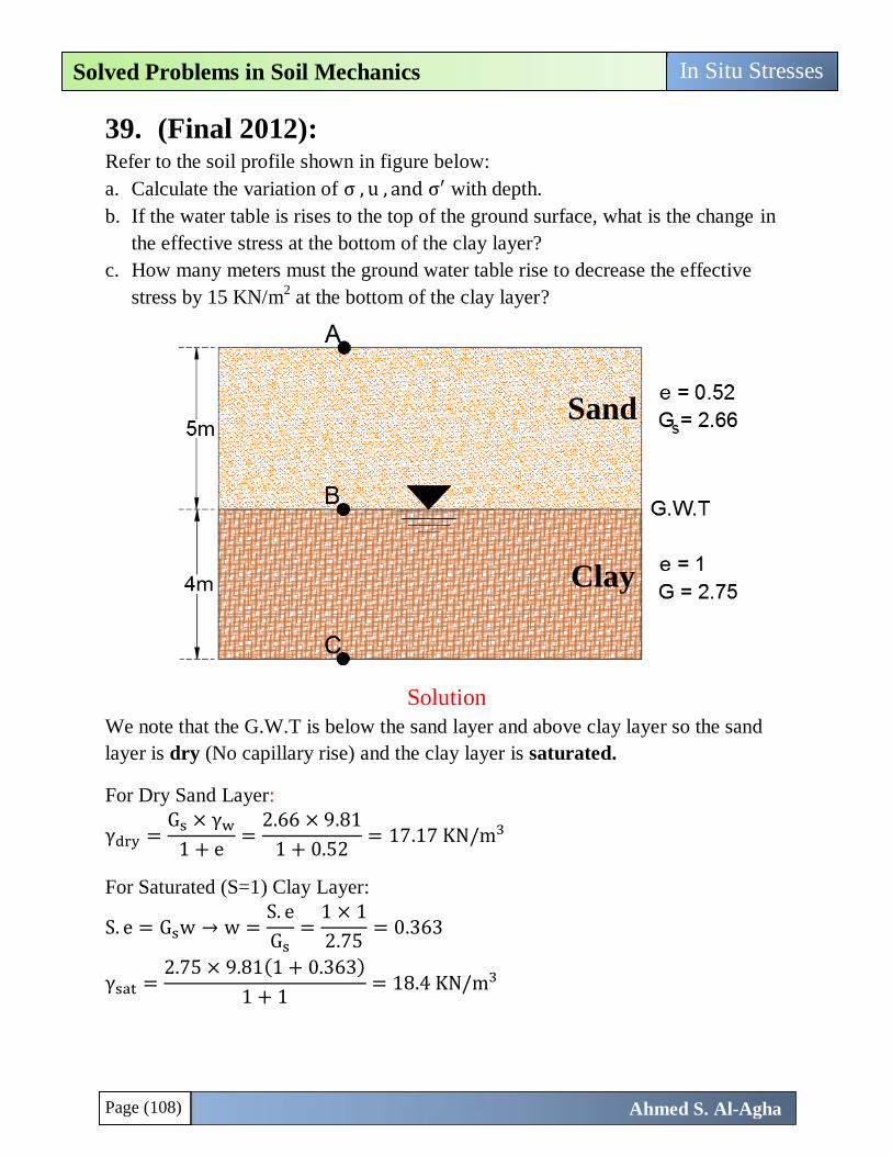
Page (108)
In Situ Stresses Solved Problems in Soil Mechanics
Ahmed S. Al-Agha
39. (Final 2012): Refer to the soil profile shown in figure below: a. Calculate the variation of σ , u , and σ′ with depth.
b. If the water table is rises to the top of the ground surface, what is the change in
the effective stress at the bottom of the clay layer?
c. How many meters must the ground water table rise to decrease the effective
stress by 15 KN/m2 at the bottom of the clay layer?
Solution
We note that the G.W.T is below the sand layer and above clay layer so the sand
layer is dry (No capillary rise) and the clay layer is saturated.
For Dry Sand Layer:
γdry =Gs × γw
1 + e=
2.66 × 9.81
1 + 0.52= 17.17 KN/m3
For Saturated (S=1) Clay Layer:
S. e = Gsw → w =S. e
Gs=
1 × 1
2.75= 0.363
γsat =2.75 × 9.81(1 + 0.363)
1 + 1= 18.4 KN/m3
Sand
Clay
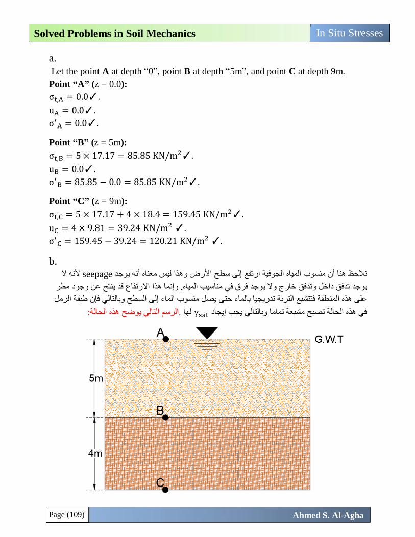
Page (109)
In Situ Stresses Solved Problems in Soil Mechanics
Ahmed S. Al-Agha
a.
Let the point A at depth “0”, point B at depth “5m”, and point C at depth 9m.
Point “A” (z = 0.0):
σt,A = 0.0✓.
uA = 0.0✓.
σ′A = 0.0✓.
Point “B” (z = 5m):
σt,B = 5 × 17.17 = 85.85 KN/m2✓.
uB = 0.0✓.
σ′B = 85.85 − 0.0 = 85.85 KN/m2✓.
Point “C” (z = 9m):
σt,C = 5 × 17.17 + 4 × 18.4 = 159.45 KN/m2✓.
uC = 4 × 9.81 = 39.24 KN/m2 ✓.
σ′C = 159.45 − 39.24 = 120.21 KN/m2 ✓.
b.
ألنه ال seepageإلى سطح األرض وهذا ليس معناه أنه يوجد ارتفعنالحظ هنا أن منسوب المياه الجوفية
قد ينتج عن وجود مطر االرتفاعتدفق داخل وتدفق خارج وال يوجد فرق في مناسيب المياه, وإنما هذا يوجد
طقة فتتشبع التربة تدريجيا بالماء حتى يصل منسوب الماء إلى السطح وبالتالي فإن طبقة الرمل على هذه المن
الرسم التالي يوضح هذه الحالة:.لها γsatفي هذه الحالة تصبح مشبعة تماما وبالتالي يجب إيجاد
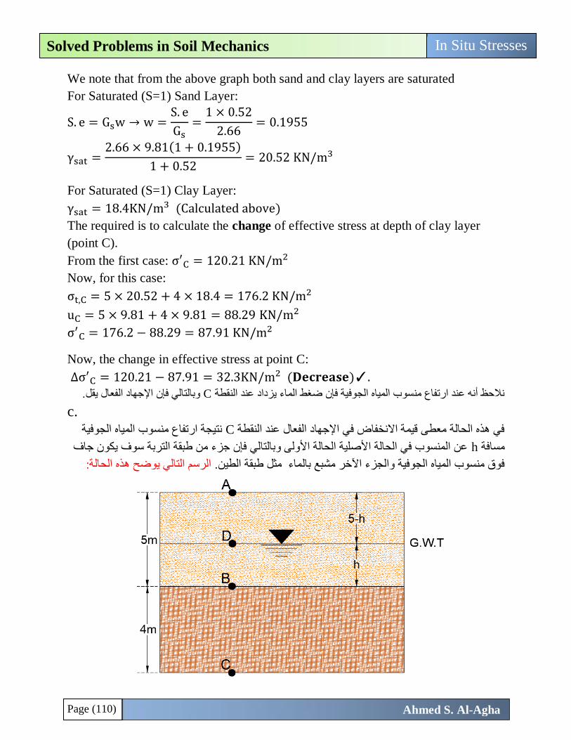
Page (110)
In Situ Stresses Solved Problems in Soil Mechanics
Ahmed S. Al-Agha
We note that from the above graph both sand and clay layers are saturated
For Saturated (S=1) Sand Layer:
S. e = Gsw → w =S. e
Gs=
1 × 0.52
2.66= 0.1955
γsat =2.66 × 9.81(1 + 0.1955)
1 + 0.52= 20.52 KN/m3
For Saturated (S=1) Clay Layer:
γsat = 18.4KN/m3 (Calculated above)
The required is to calculate the change of effective stress at depth of clay layer
(point C).
From the first case: σ′C = 120.21 KN/m2
Now, for this case:
σt,C = 5 × 20.52 + 4 × 18.4 = 176.2 KN/m2
uC = 5 × 9.81 + 4 × 9.81 = 88.29 KN/m2
σ′C = 176.2 − 88.29 = 87.91 KN/m2
Now, the change in effective stress at point C:
∆σ′C = 120.21 − 87.91 = 32.3KN/m2 (𝐃𝐞𝐜𝐫𝐞𝐚𝐬𝐞)✓.
ل.وبالتالي فإن اإلجهاد الفعال يق Cنالحظ أنه عند ارتفاع منسوب المياه الجوفية فإن ضغط الماء يزداد عند النقطة
c.
نتيجة ارتفاع منسوب المياه الجوفية Cفي هذه الحالة معطى قيمة االنخفاض في اإلجهاد الفعال عند النقطة
عن المنسوب في الحالة األصلية الحالة األولى وبالتالي فإن جزء من طبقة التربة سوف يكون جاف hمسافة
الرسم التالي يوضح هذه الحالة: .بالماء مثل طبقة الطينفوق منسوب المياه الجوفية والجزء اآلخر مشبع
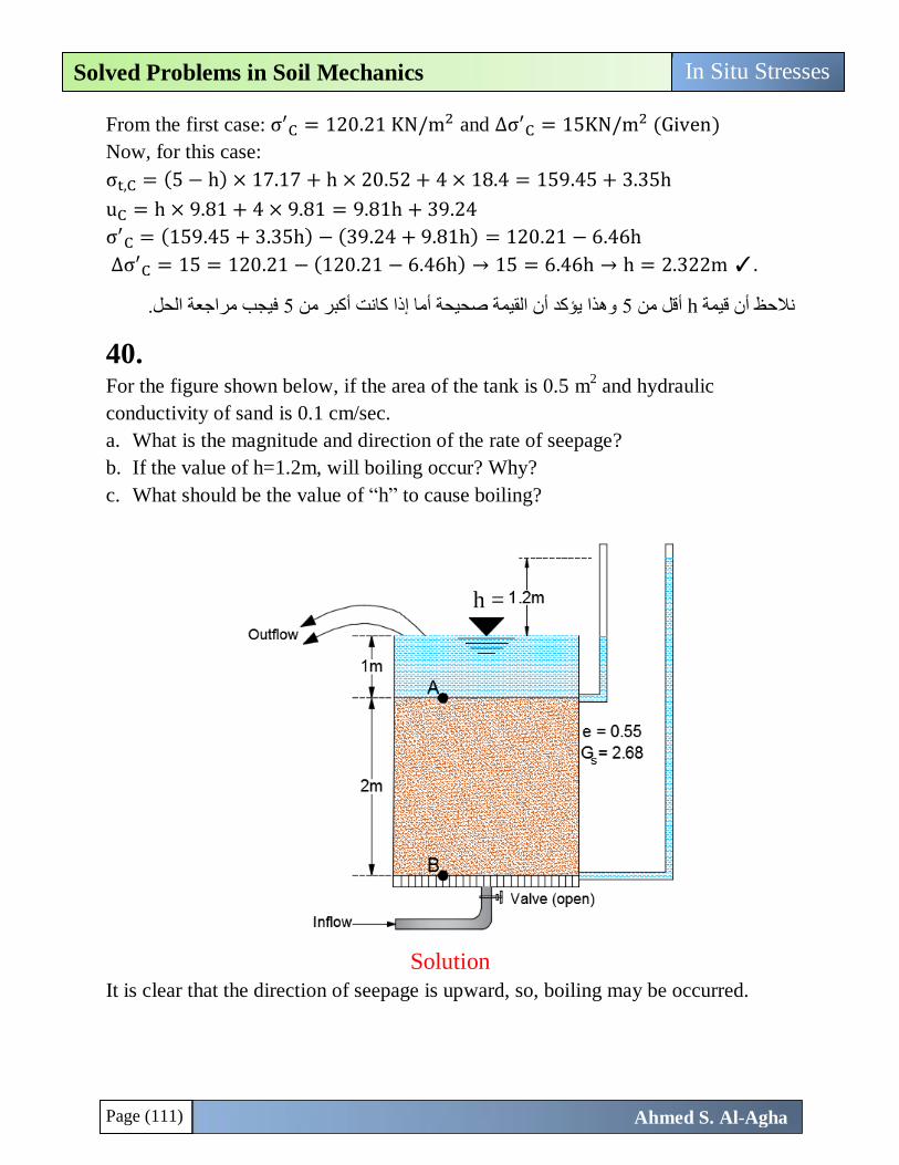
Page (111)
In Situ Stresses Solved Problems in Soil Mechanics
Ahmed S. Al-Agha
From the first case: σ′C = 120.21 KN/m2 and ∆σ′
C = 15KN/m2 (Given)
Now, for this case:
σt,C = (5 − h) × 17.17 + h × 20.52 + 4 × 18.4 = 159.45 + 3.35h
uC = h × 9.81 + 4 × 9.81 = 9.81h + 39.24
σ′C = (159.45 + 3.35h) − (39.24 + 9.81h) = 120.21 − 6.46h
∆σ′C = 15 = 120.21 − (120.21 − 6.46h) → 15 = 6.46h → h = 2.322m ✓.
فيجب مراجعة الحل. 5وهذا يؤكد أن القيمة صحيحة أما إذا كانت أكبر من 5أقل من hنالحظ أن قيمة
40. For the figure shown below, if the area of the tank is 0.5 m
2 and hydraulic
conductivity of sand is 0.1 cm/sec.
a. What is the magnitude and direction of the rate of seepage?
b. If the value of h=1.2m, will boiling occur? Why?
c. What should be the value of “h” to cause boiling?
Solution
It is clear that the direction of seepage is upward, so, boiling may be occurred.
h =
Page (112)
In Situ Stresses Solved Problems in Soil Mechanics
Ahmed S. Al-Agha
a.
q = KiA , K = 0.1 × 10⁻² m/ sec , A = 0.5m2
i =Total Losses
Length of Soil=
1.2
2= 0.6
q = 0.1 × 10−2 × 0.6 × 0.5 = 3 × 10⁻⁴ m3/ sec (Upward)✓.
b.
Always we check stability at the point having maximum pressure head because it
have maximum pore water pressure and minimum effective stress.
So, we want to calculate the effective stress at point (B), if the value is negative,
the boiling will occur, otherwise, the boiling will not occur.
Firstly, we calculate the saturated unit weight for the soil:
S. e = Gsw → w =S. e
Gs=
1 × 0.55
2.68= 0.2052
γsat =2.68 × 9.81(1 + 0.2052)
1 + 0.55= 20.44 KN/m3
σt,B = 1 × 9.81 + 2 × 20.44 = 50.69 KN/m2
uB = 1 × 9.81 + 2 × 9.81 + 1.2 × 9.81 = 41.202KN/m2
σ′B = 50.69 − 41.202 = 9.488 KN/m2 > 0 → boiling will not occur✓.
c.
The value of (h) that causes boiling must be greater than the critical value of h
(σ′B = 0)
σt,B = 1 × 9.81 + 2 × 20.44 = 50.69 KN/m2
uB = 1 × 9.81 + 2 × 9.81 + h × 9.81 = 29.43 + 9.81 h
Critical case occur when σ′B = 0 → σt,B = uB
50.69 = 29.43 + 9.81 h → h = 2.167m
So, the value of “h” that cause boiling must be larger than 2.167 m
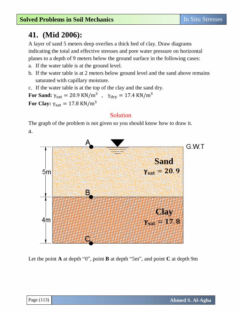
Page (113)
In Situ Stresses Solved Problems in Soil Mechanics
Ahmed S. Al-Agha
41. (Mid 2006): A layer of sand 5 meters deep overlies a thick bed of clay. Draw diagrams
indicating the total and effective stresses and pore water pressure on horizontal
planes to a depth of 9 meters below the ground surface in the following cases:
a. If the water table is at the ground level.
b. If the water table is at 2 meters below ground level and the sand above remains
saturated with capillary moisture.
c. If the water table is at the top of the clay and the sand dry.
For Sand: γsat = 20.9 KN/m3 , γdry = 17.4 KN/m3
For Clay: γsat = 17.8 KN/m3
Solution
The graph of the problem is not given so you should know how to draw it.
a.
Let the point A at depth “0”, point B at depth “5m”, and point C at depth 9m
Sand
Clay
𝛄𝐬𝐚𝐭 = 𝟐𝟎. 𝟗
𝛄𝐬𝐚𝐭 = 𝟏𝟕. 𝟖
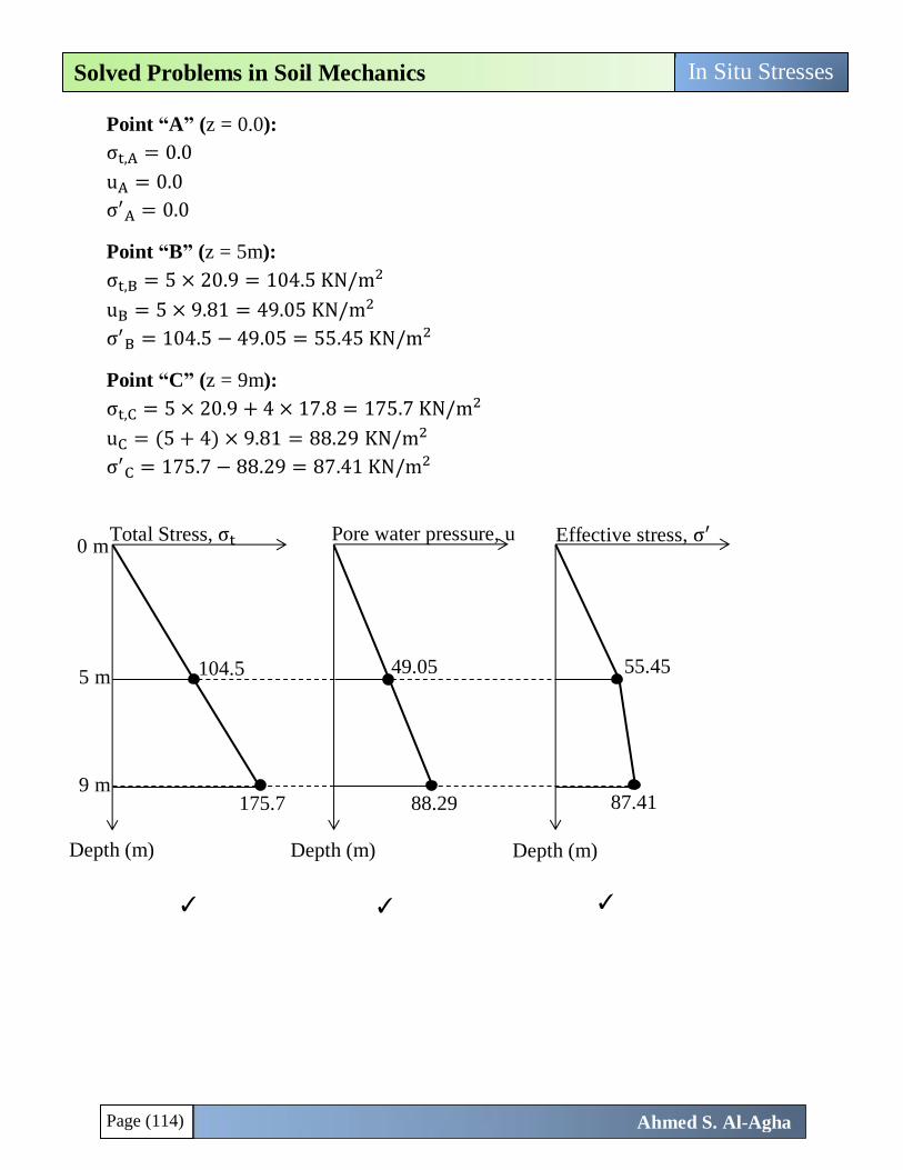
Page (114)
In Situ Stresses Solved Problems in Soil Mechanics
Ahmed S. Al-Agha
Point “A” (z = 0.0):
σt,A = 0.0
uA = 0.0
σ′A = 0.0
Point “B” (z = 5m):
σt,B = 5 × 20.9 = 104.5 KN/m2
uB = 5 × 9.81 = 49.05 KN/m2
σ′B = 104.5 − 49.05 = 55.45 KN/m2
Point “C” (z = 9m):
σt,C = 5 × 20.9 + 4 × 17.8 = 175.7 KN/m2
uC = (5 + 4) × 9.81 = 88.29 KN/m2
σ′C = 175.7 − 88.29 = 87.41 KN/m2
Total Stress, σt
Depth (m)
Pore water pressure, u Effective stress, σ′
Depth (m) Depth (m)
0 m
5 m
9 m 175.7
104.5 49.05 55.45
87.41 88.29
✓ ✓ ✓
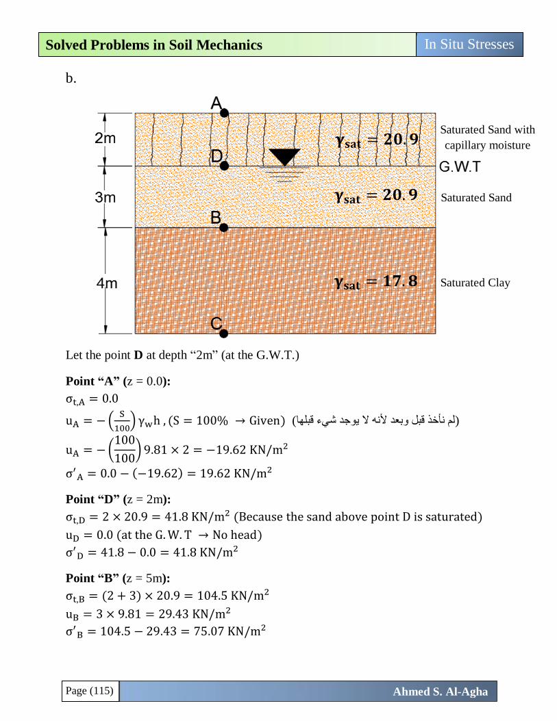
Page (115)
In Situ Stresses Solved Problems in Soil Mechanics
Ahmed S. Al-Agha
b.
Let the point D at depth “2m” (at the G.W.T.)
Point “A” (z = 0.0):
σt,A = 0.0
uA = − (S
100) γwh , (S = 100% → Given) ( يء قبلهالم نأخذ قبل وبعد ألنه ال يوجد ش )
uA = − (100
100) 9.81 × 2 = −19.62 KN/m2
σ′A = 0.0 − (−19.62) = 19.62 KN/m2
Point “D” (z = 2m):
σt,D = 2 × 20.9 = 41.8 KN/m2 (Because the sand above point D is saturated)
uD = 0.0 (at the G. W. T → No head)
σ′D = 41.8 − 0.0 = 41.8 KN/m2
Point “B” (z = 5m):
σt,B = (2 + 3) × 20.9 = 104.5 KN/m2
uB = 3 × 9.81 = 29.43 KN/m2
σ′B = 104.5 − 29.43 = 75.07 KN/m2
Saturated Sand with
capillary moisture
Saturated Sand
Saturated Clay 𝛄𝐬𝐚𝐭 = 𝟏𝟕. 𝟖
𝛄𝐬𝐚𝐭 = 𝟐𝟎. 𝟗
𝛄𝐬𝐚𝐭 = 𝟐𝟎. 𝟗
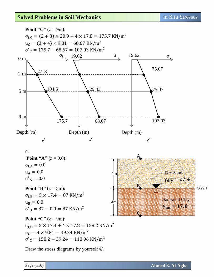
Page (116)
In Situ Stresses Solved Problems in Soil Mechanics
Ahmed S. Al-Agha
Point “C” (z = 9m):
σt,C = (2 + 3) × 20.9 + 4 × 17.8 = 175.7 KN/m2
uC = (3 + 4) × 9.81 = 68.67 KN/m2
σ′C = 175.7 − 68.67 = 107.03 KN/m2
c.
Point “A” (z = 0.0):
σt,A = 0.0
uA = 0.0
σ′A = 0.0
Point “B” (z = 5m):
σt,B = 5 × 17.4 = 87 KN/m2
uB = 0.0
σ′B = 87 − 0.0 = 87 KN/m2
Point “C” (z = 9m):
σt,C = 5 × 17.4 + 4 × 17.8 = 158.2 KN/m2
uC = 4 × 9.81 = 39.24 KN/m2
σ′C = 158.2 − 39.24 = 118.96 KN/m2
Draw the stress diagrams by yourself .
σt
Depth (m)
u σ′
Depth (m) Depth (m)
0 m
5 m
9 m 175.7
104.5 29.43 75.07
45
107.03 68.67
2 m 41.8
19.62 19.62
75.07
45
✓ ✓ ✓
Saturated Clay
Dry Sand
𝛄𝐬𝐚𝐭 = 𝟏𝟕. 𝟖
𝛄𝐝𝐫𝐲 = 𝟏𝟕. 𝟒
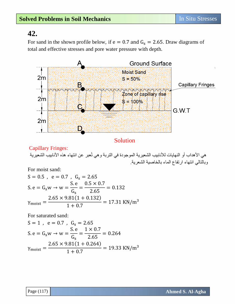
Page (117)
In Situ Stresses Solved Problems in Soil Mechanics
Ahmed S. Al-Agha
42.
For sand in the shown profile below, if e = 0.7 and Gs = 2.65. Draw diagrams of
total and effective stresses and pore water pressure with depth.
Solution
Capillary Fringes:
هذه األنابيب الشعيرية انتهاءعبر عن هي األهداب أو النهايات لألنابيب الشعيرية الموجودة في التربة وهي ت
.انتهاء ارتفاع الماء بالخاصية الشعريةوبالتالي
For moist sand:
S = 0.5 , e = 0.7 , Gs = 2.65
S. e = Gsw → w =S. e
Gs=
0.5 × 0.7
2.65= 0.132
γmoist =2.65 × 9.81(1 + 0.132)
1 + 0.7= 17.31 KN/m3
For saturated sand:
S = 1 , e = 0.7 , Gs = 2.65
S. e = Gsw → w =S. e
Gs=
1 × 0.7
2.65= 0.264
γmoist =2.65 × 9.81(1 + 0.264)
1 + 0.7= 19.33 KN/m3
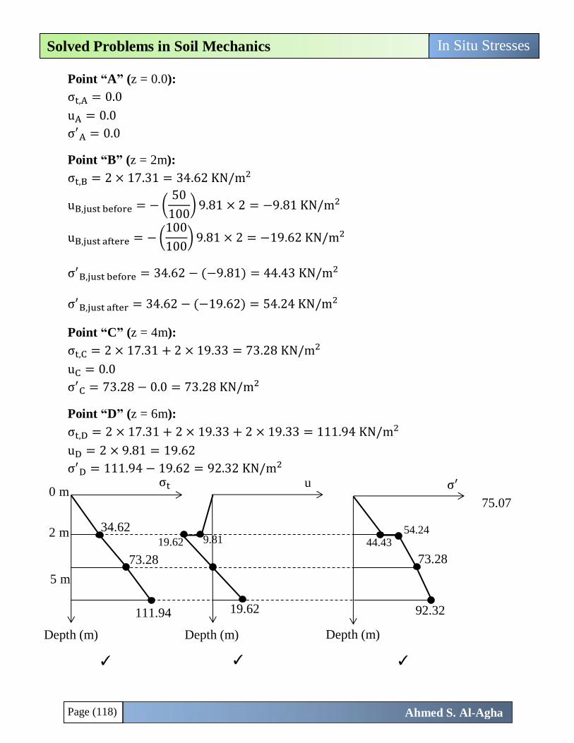
Page (118)
In Situ Stresses Solved Problems in Soil Mechanics
Ahmed S. Al-Agha
Point “A” (z = 0.0):
σt,A = 0.0
uA = 0.0
σ′A = 0.0
Point “B” (z = 2m):
σt,B = 2 × 17.31 = 34.62 KN/m2
uB,just before = − (50
100) 9.81 × 2 = −9.81 KN/m2
uB,just aftere = − (100
100) 9.81 × 2 = −19.62 KN/m2
σ′B,just before = 34.62 − (−9.81) = 44.43 KN/m2
σ′B,just after = 34.62 − (−19.62) = 54.24 KN/m2
Point “C” (z = 4m):
σt,C = 2 × 17.31 + 2 × 19.33 = 73.28 KN/m2
uC = 0.0
σ′C = 73.28 − 0.0 = 73.28 KN/m2
Point “D” (z = 6m):
σt,D = 2 × 17.31 + 2 × 19.33 + 2 × 19.33 = 111.94 KN/m2
uD = 2 × 9.81 = 19.62
σ′D = 111.94 − 19.62 = 92.32 KN/m2
σt
Depth (m)
u σ′
Depth (m) Depth (m)
0 m
5 m
19.62
2 m 34.62
75.07
45
73.28
111.94 73.28 73.28
9.81 19.62
73.28 73.28 73.28 73.28
73.28 73.28
73.28 73.28
73.28 73.28
73.28 73.28
73.28 73.28
73.28 73.28
92.32
73.28
44.43 54.24
✓ ✓ ✓
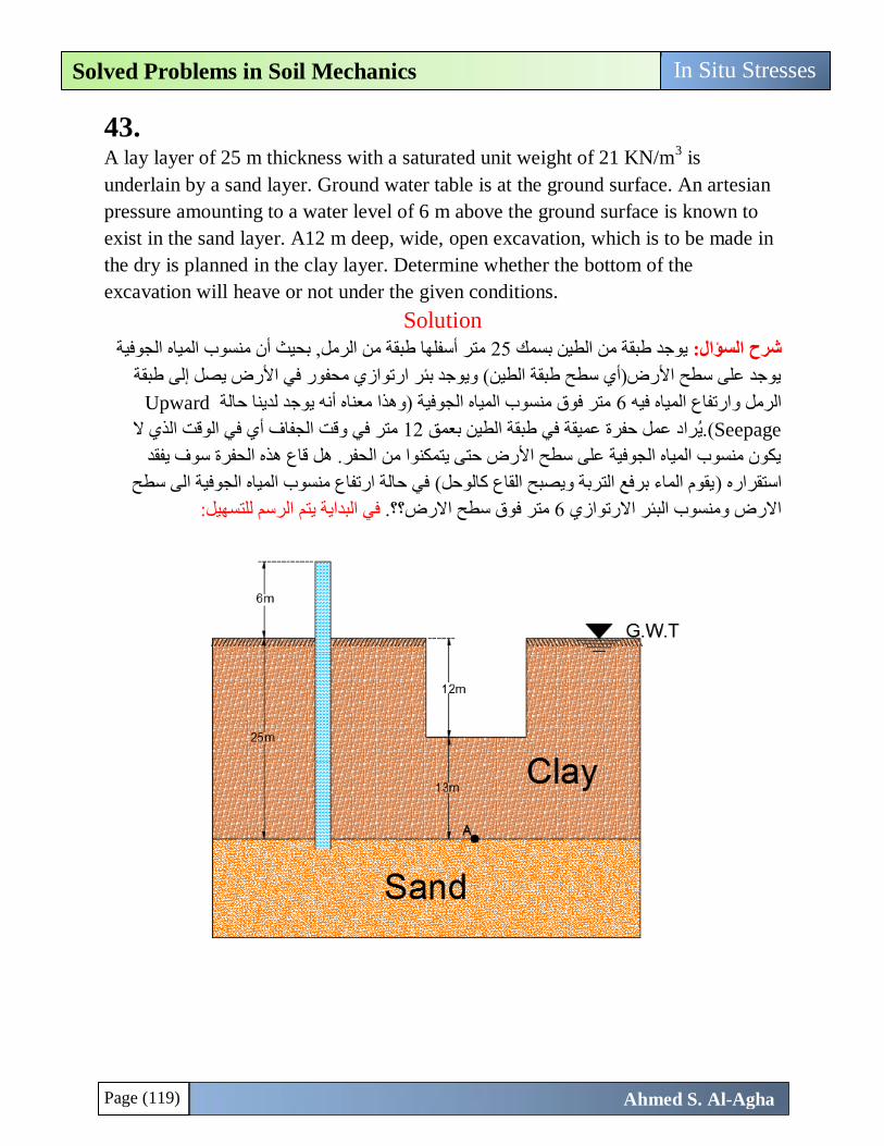
Page (119)
In Situ Stresses Solved Problems in Soil Mechanics
Ahmed S. Al-Agha
43.
A lay layer of 25 m thickness with a saturated unit weight of 21 KN/m3 is
underlain by a sand layer. Ground water table is at the ground surface. An artesian
pressure amounting to a water level of 6 m above the ground surface is known to
exist in the sand layer. A12 m deep, wide, open excavation, which is to be made in
the dry is planned in the clay layer. Determine whether the bottom of the
excavation will heave or not under the given conditions.
Solution
متر أسفلها طبقة من الرمل, بحيث أن منسوب المياه الجوفية 25يوجد طبقة من الطين بسمك :شرح السؤال
ة يوجد على سطح األرض)أي سطح طبقة الطين( ويوجد بئر ارتوازي محفور في األرض يصل إلى طبق
Upwardمتر فوق منسوب المياه الجوفية )وهذا معناه أنه يوجد لدينا حالة 6الرمل وارتفاع المياه فيه
Seepage متر في وقت الجفاف أي في الوقت الذي ال 12راد عمل حفرة عميقة في طبقة الطين بعمق (.ي
هذه الحفرة سوف يفقد يكون منسوب المياه الجوفية على سطح األرض حتى يتمكنوا من الحفر. هل قاع
يقوم الماء برفع التربة ويصبح القاع كالوحل( في حالة ارتفاع منسوب المياه الجوفية الى سطح استقراره )
الرسم للتسهيل:في البداية يتم . ؟؟متر فوق سطح االرض 6االرض ومنسوب البئر االرتوازي
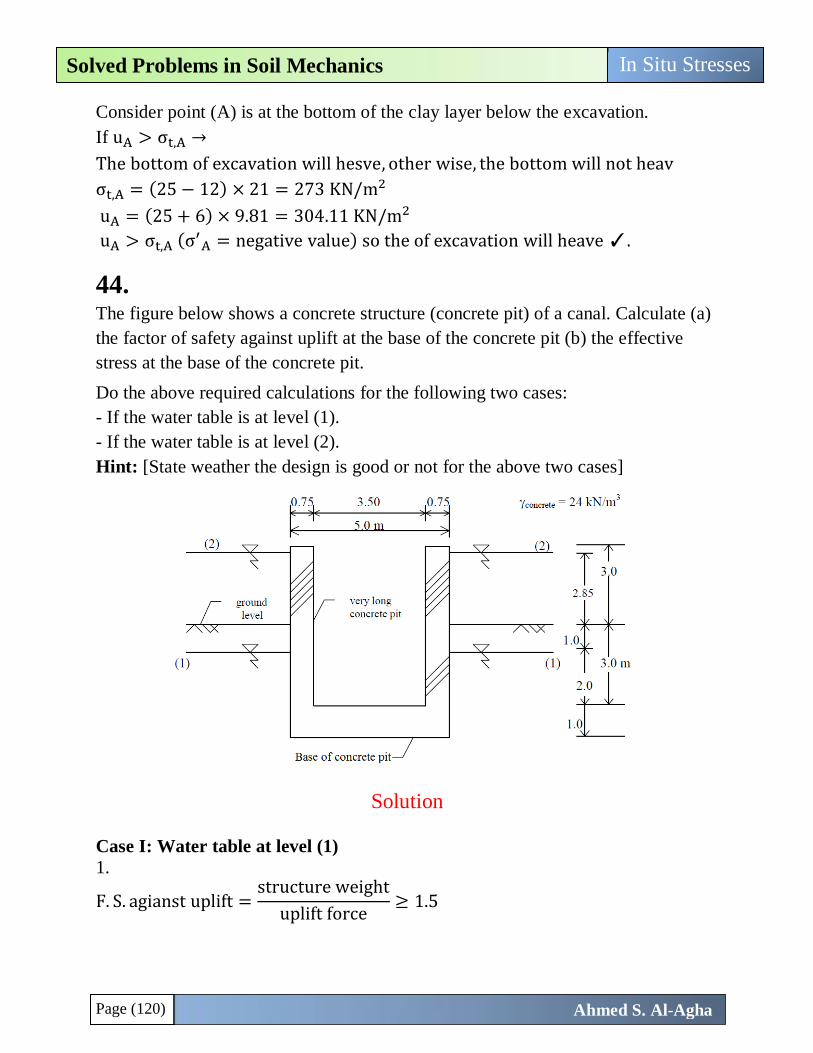
Page (120)
In Situ Stresses Solved Problems in Soil Mechanics
Ahmed S. Al-Agha
Consider point (A) is at the bottom of the clay layer below the excavation.
If uA > σt,A →
The bottom of excavation will hesve, other wise, the bottom will not heav
σt,A = (25 − 12) × 21 = 273 KN/m2
uA = (25 + 6) × 9.81 = 304.11 KN/m2
uA > σt,A (σ′A = negative value) so the of excavation will heave ✓.
44.
The figure below shows a concrete structure (concrete pit) of a canal. Calculate (a)
the factor of safety against uplift at the base of the concrete pit (b) the effective
stress at the base of the concrete pit.
Do the above required calculations for the following two cases:
- If the water table is at level (1).
- If the water table is at level (2).
Hint: [State weather the design is good or not for the above two cases]
Solution
Case I: Water table at level (1)
1.
F. S. agianst uplift =structure weight
uplift force≥ 1.5
Page (121)
In Situ Stresses Solved Problems in Soil Mechanics
Ahmed S. Al-Agha
structure weight = Vstructure × γconcrete
Vstructure = Vbox − Vspace = (7 × 5) − (6 × 3.5) = 14 m3
→ structure weight = 14 × 24 = 336 kN
uplift force = u@base × base area
u@base = γw × hw,above base = 10 × 3 = 30 kN/m2
uplift force = 30 × (5 × 1) = 150 kN.
F. S. =336
150= 2.24 > 1.5 → The design is good in this case ✓.
2.
σ@base′ = qstructure − u@base =
336
(5 × 1)− 30 = 37.2 kN/m2✓.
Case II: Water table at level (2)
1.
structure weight = 336 kN
uplift force = u@base × base area
u@base = γw × hw,above base = 10 × 6.85 = 68.5 kN/m2
uplift force = 68.5 × (5 × 1) = 342.5 kN.
F. S. =336
342.5= 0.98 < 1.5 → The design is not good in this case ✓.
2.
σ@base′ = qstructure − u@base =
336
(5 × 1)− 68.5 = −1.3 ≅ 0.0 ✓.
→ this means the structure weight equals uplift force
→ Soil does not carry any load and the structure will float
Chapter (10)
Stresses in a Soil Mass
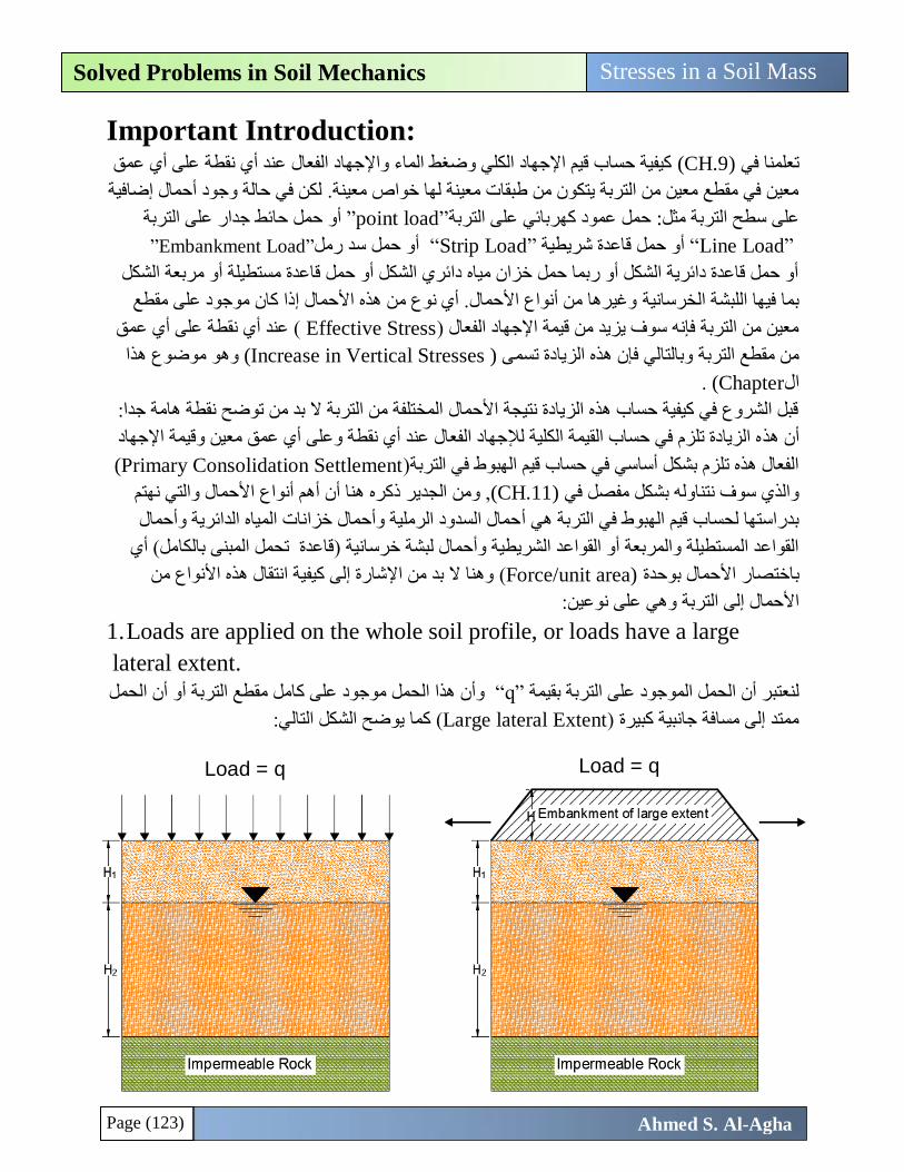
Page (123)
Stresses in a Soil Mass Solved Problems in Soil Mechanics
Ahmed S. Al-Agha
Important Introduction:
على أي عمق كيفية حساب قيم اإلجهاد الكلي وضغط الماء واإلجهاد الفعال عند أي نقطة (CH.9)تعلمنا في
لكن في حالة وجود أحمال إضافية معين في مقطع معين من التربة يتكون من طبقات معينة لها خواص معينة.
جدار على التربةأو حمل حائط ”point load”حمل عمود كهربائي على التربة :على سطح التربة مثل
“Line Load” أو حمل قاعدة شريطية “Strip Load” أو حمل سد رمل”Embankment Load”
أو حمل قاعدة دائرية الشكل أو ربما حمل خزان مياه دائري الشكل أو حمل قاعدة مستطيلة أو مربعة الشكل
وغيرها من أنواع األحمال. أي نوع من هذه األحمال إذا كان موجود على مقطع بما فيها اللبشة الخرسانية
( عند أي نقطة على أي عمق Effective Stressعال )معين من التربة فإنه سوف يزيد من قيمة اإلجهاد الف
وهو موضوع هذا ( Increase in Vertical Stresses)وبالتالي فإن هذه الزيادة تسمى من مقطع التربة
. Chapter)ال
قبل الشروع في كيفية حساب هذه الزيادة نتيجة األحمال المختلفة من التربة ال بد من توضح نقطة هامة جدا:
ه الزيادة تلزم في حساب القيمة الكلية لإلجهاد الفعال عند أي نقطة وعلى أي عمق معين وقيمة اإلجهاد هذأن
Primary Consolidation Settlement)الفعال هذه تلزم بشكل أساسي في حساب قيم الهبوط في التربة)
األحمال والتي نهتم عالجدير ذكره هنا أن أهم أنوا , ومن(CH.11)والذي سوف نتناوله بشكل مفصل في
حمال السدود الرملية وأحمال خزانات المياه الدائرية وأحمال أبدراستها لحساب قيم الهبوط في التربة هي
كامل( أي بالمبنى التحمل قاعدة ) القواعد المستطيلة والمربعة أو القواعد الشريطية وأحمال لبشة خرسانية
وهنا ال بد من اإلشارة إلى كيفية انتقال هذه األنواع من ((Force/unit areaاألحمال بوحدة باختصار
وهي على نوعين:األحمال إلى التربة
1. Loads are applied on the whole soil profile, or loads have a large
lateral extent.
أو أن الحمل ل مقطع التربة وأن هذا الحمل موجود على كام q“ ” لنعتبر أن الحمل الموجود على التربة بقيمة
يوضح الشكل التالي: كما (Large lateral Extentممتد إلى مسافة جانبية كبيرة )
Load = q Load = q
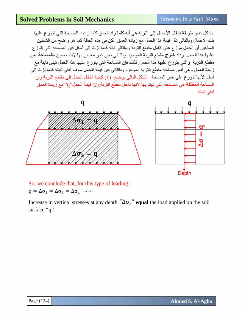
Page (124)
Stresses in a Soil Mass Solved Problems in Soil Mechanics
Ahmed S. Al-Agha
وزع عليها تتإلى التربة هي أنه كلما زاد العمق كلما زادت المساحة التي األحمالنتقال إطريقة بشكل عام,
. لكن في هذه الحالة كما هو واضح من الشكلين لعمقتلك األحمال وبالتالي تقل قيمة هذا الحمل مع زيادة ا
لنا إلى أسفل فإن المساحة التي يتوزع زالسابقين أن الحمل موزع على كامل مقطع التربة وبالتالي فإنه كلما ن
بالمساحة من ألننا معنيين بها وبالتالي نحن غير معنيين مقطع التربة الموجود خارجاد دعليها هذا الحمل تز
مع التي يتوزع عليها هذا الحمل, لذلك فإن المساحة التي يتوزع عليها هذا الحمل تبقى ثابتةو تربة مقطع ال
ثابتة كلما نزلنا إلى ىوبالتالي فإن قيمة الحمل سوف تبق وهي نفس مساحة مقطع التربة الموجود زيادة العمق
انتقال الحمل إلى مقطع التربة وأن كيفية (1) :يوضح يالتال الشكل .أسفل ألنها تتوزع على نفس المساحة
مع زيادة العمق ”q”( قيمة الحمل2احة التي نهتم بها ألنها داخل مقطع التربة.)مسهي ال المظللةالمساحة
ثابتة. ىتبق
So, we conclude that, for this type of loading:
q = ∆σ1 = ∆σ2 = ∆σz →→
Increase in vertical stresses at any depth equal the load applied on the soil
surface “q”.
∆𝛔𝟏 = 𝐪
q
∆𝛔𝟐 = 𝐪
∆𝛔
=𝐪
q
“∆σ𝑧”
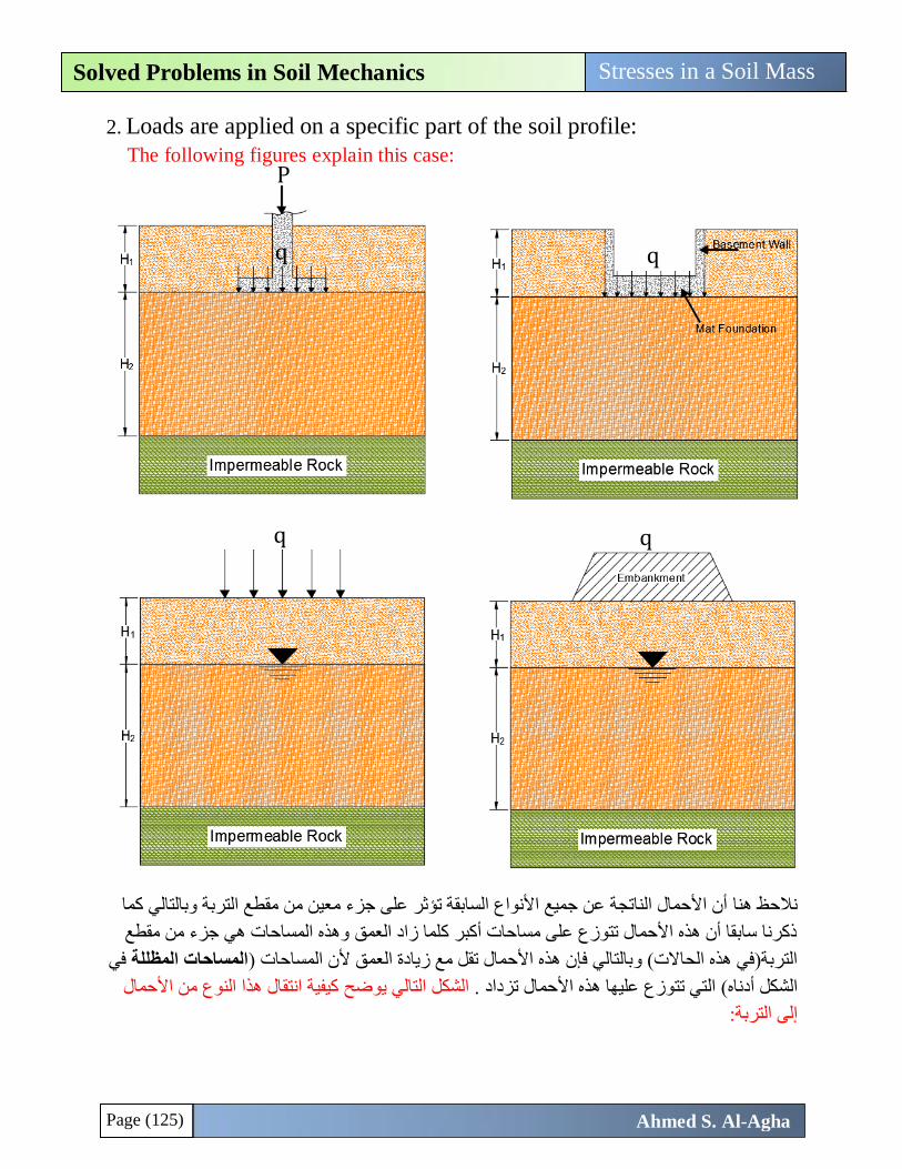
Page (125)
Stresses in a Soil Mass Solved Problems in Soil Mechanics
Ahmed S. Al-Agha
2. Loads are applied on a specific part of the soil profile:
The following figures explain this case:
عين من مقطع التربة وبالتالي كما أن األحمال الناتجة عن جميع األنواع السابقة تؤثر على جزء منالحظ هنا
وهذه المساحات هي جزء من مقطع ذكرنا سابقا أن هذه األحمال تتوزع على مساحات أكبر كلما زاد العمق
في المساحات المظللة) ن هذه األحمال تقل مع زيادة العمق ألن المساحاتإالتربة)في هذه الحاالت( وبالتالي ف
كيفية انتقال هذا النوع من األحمال الشكل التالي يوضح . تزدادهذه األحمال التي تتوزع عليها الشكل أدناه(
إلى التربة:
q
P
q
q q
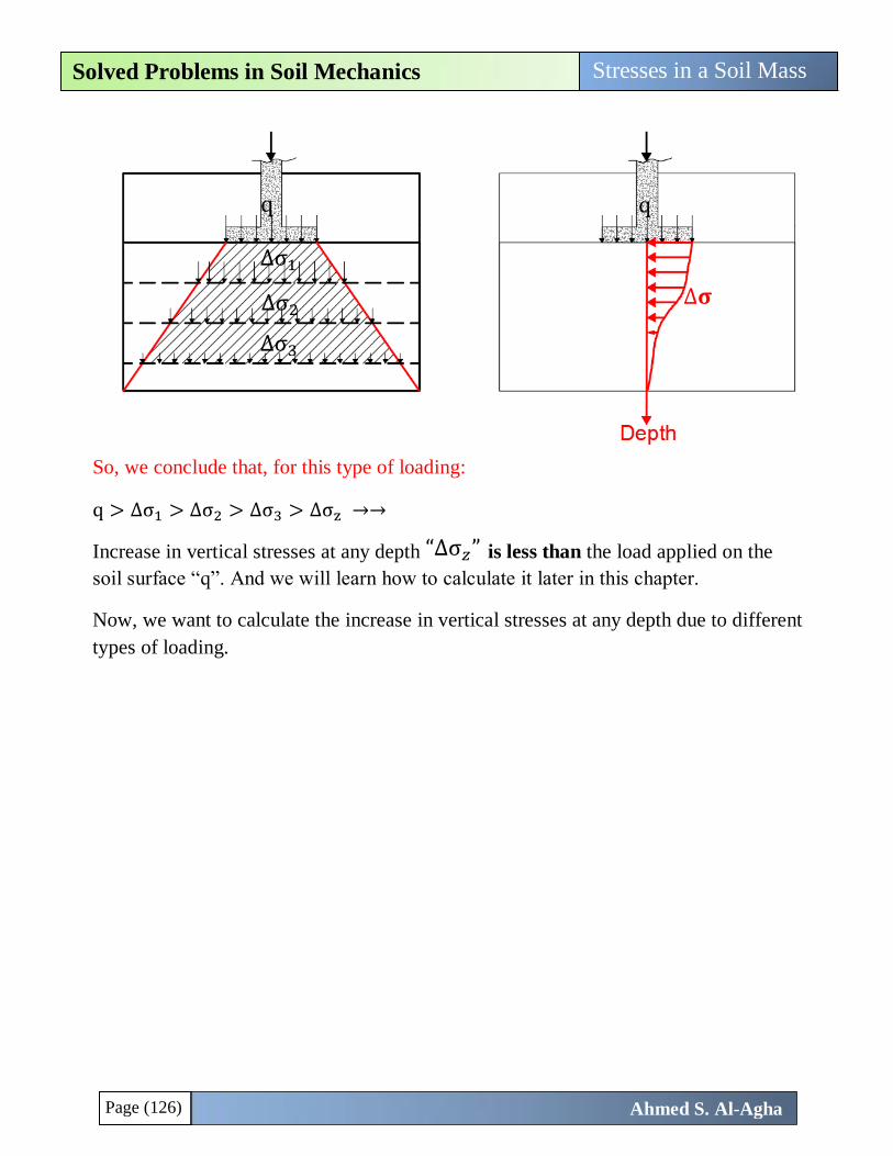
Page (126)
Stresses in a Soil Mass Solved Problems in Soil Mechanics
Ahmed S. Al-Agha
∆σ1
q
∆σ2
∆σ3
q
∆𝛔
“∆σ𝑧”
So, we conclude that, for this type of loading:
q > ∆σ1 > ∆σ2 > ∆σ3 > ∆σz →→
Increase in vertical stresses at any depth is less than the load applied on the
soil surface “q”. And we will learn how to calculate it later in this chapter.
Now, we want to calculate the increase in vertical stresses at any depth due to different
types of loading.
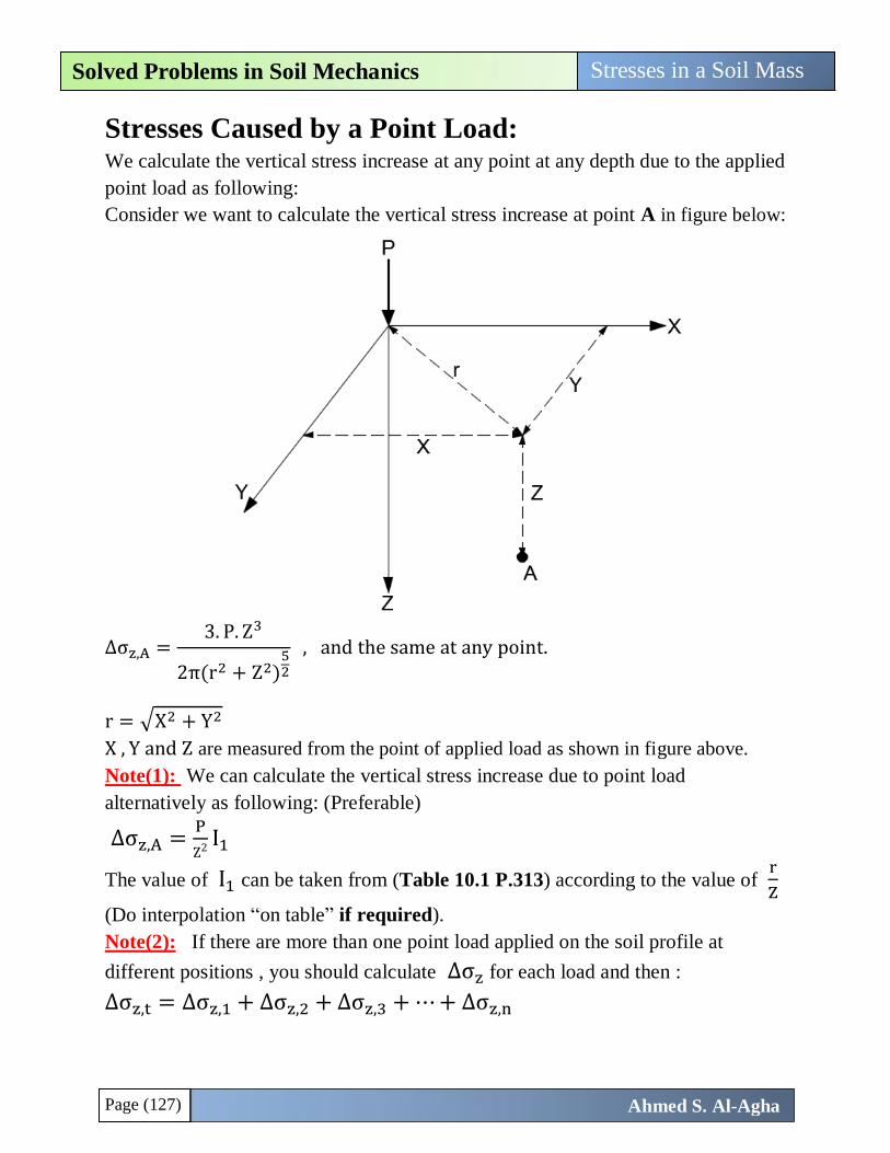
Page (127)
Stresses in a Soil Mass Solved Problems in Soil Mechanics
Ahmed S. Al-Agha
Stresses Caused by a Point Load: We calculate the vertical stress increase at any point at any depth due to the applied
point load as following:
Consider we want to calculate the vertical stress increase at point A in figure below:
∆σz,A =3. P. Z3
2π(r2 + Z2)52
, and the same at any point.
r = √X2 + Y2
X , Y and Z are measured from the point of applied load as shown in figure above. Note(1): We can calculate the vertical stress increase due to point load
alternatively as following: (Preferable)
∆σz,A =P
Z2I1
The value of I1 can be taken from (Table 10.1 P.313) according to the value of r
Z
(Do interpolation “on table” if required).
Note(2): If there are more than one point load applied on the soil profile at
different positions , you should calculate ∆σz for each load and then :
∆σz,t = ∆σz,1 + ∆σz,2 + ∆σz,3 + ⋯ + ∆σz,n
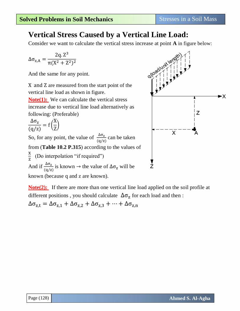
Page (128)
Stresses in a Soil Mass Solved Problems in Soil Mechanics
Ahmed S. Al-Agha
Vertical Stress Caused by a Vertical Line Load: Consider we want to calculate the vertical stress increase at point A in figure below:
∆σz,A =2q. Z3
π(X2 + Z2)2
And the same for any point.
X and Z are measured from the start point of the
vertical line load as shown in figure. Note(1): We can calculate the vertical stress
increase due to vertical line load alternatively as
following: (Preferable)
∆σz
(q/z)= f (
X
Z)
So, for any point, the value of ∆σz
(q/z) can be taken
from (Table 10.2 P.315) according to the values of X
Z (Do interpolation “if required”)
And if ∆σz
(q/z) is known → the value of ∆σz will be
known (because q and z are known).
Note(2): If there are more than one vertical line load applied on the soil profile at
different positions , you should calculate ∆σz for each load and then :
∆σz,t = ∆σz,1 + ∆σz,2 + ∆σz,3 + ⋯ + ∆σz,n
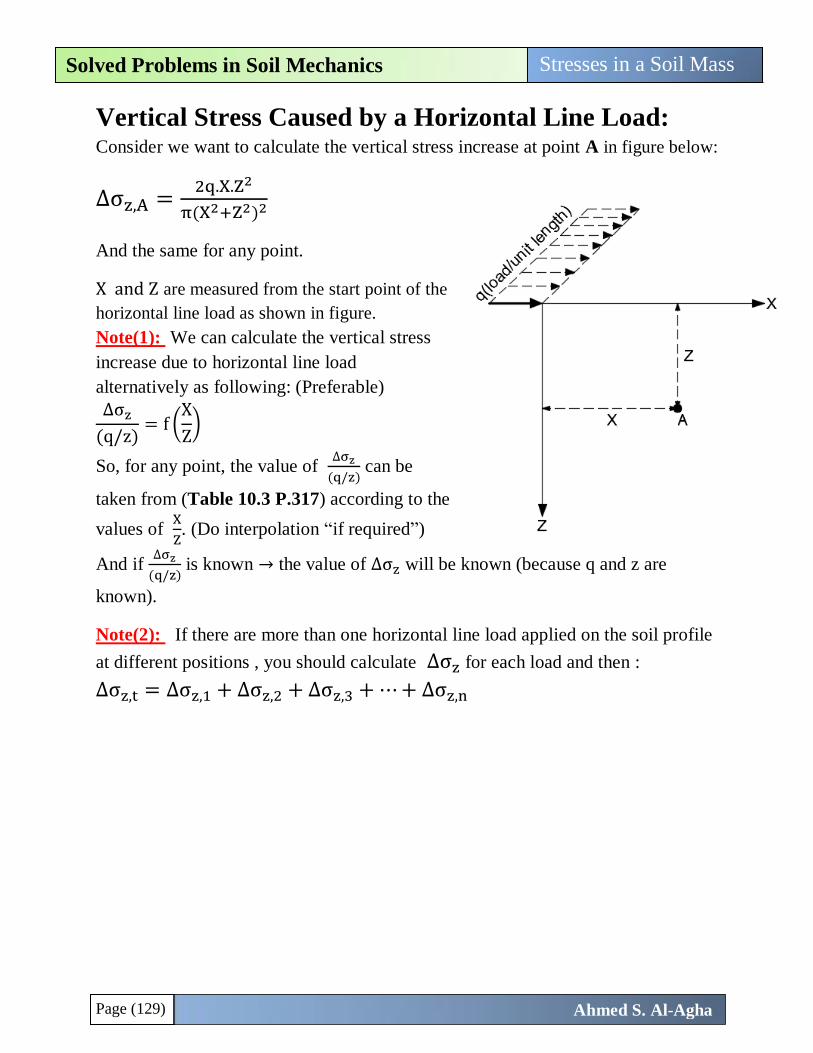
Page (129)
Stresses in a Soil Mass Solved Problems in Soil Mechanics
Ahmed S. Al-Agha
Vertical Stress Caused by a Horizontal Line Load: Consider we want to calculate the vertical stress increase at point A in figure below:
∆σz,A =2q.X.Z2
π(X2+Z2)2
And the same for any point.
X and Z are measured from the start point of the
horizontal line load as shown in figure. Note(1): We can calculate the vertical stress
increase due to horizontal line load
alternatively as following: (Preferable)
∆σz
(q/z)= f (
X
Z)
So, for any point, the value of ∆σz
(q/z) can be
taken from (Table 10.3 P.317) according to the
values of X
Z. (Do interpolation “if required”)
And if ∆σz
(q/z) is known → the value of ∆σz will be known (because q and z are
known).
Note(2): If there are more than one horizontal line load applied on the soil profile
at different positions , you should calculate ∆σz for each load and then :
∆σz,t = ∆σz,1 + ∆σz,2 + ∆σz,3 + ⋯ + ∆σz,n
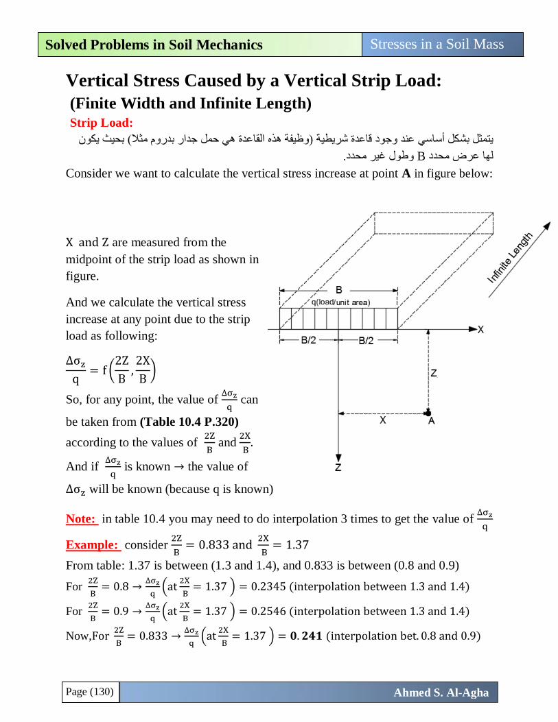
Page (130)
Stresses in a Soil Mass Solved Problems in Soil Mechanics
Ahmed S. Al-Agha
Vertical Stress Caused by a Vertical Strip Load:
(Finite Width and Infinite Length) Strip Load:
جدار بدروم مثال( بحيث يكون )وظيفة هذه القاعدة هي حمل يتمثل بشكل أساسي عند وجود قاعدة شريطية
وطول غير محدد. Bلها عرض محدد
Consider we want to calculate the vertical stress increase at point A in figure below:
X and Z are measured from the
midpoint of the strip load as shown in
figure.
And we calculate the vertical stress
increase at any point due to the strip
load as following:
∆σz
q= f (
2Z
B,2X
B)
So, for any point, the value of ∆σz
q can
be taken from (Table 10.4 P.320)
according to the values of 2Z
B and
2X
B.
And if ∆σz
q is known → the value of
∆σz will be known (because q is known)
Note: in table 10.4 you may need to do interpolation 3 times to get the value of ∆σz
q
Example: consider 2Z
B= 0.833 and
2X
B= 1.37
From table: 1.37 is between (1.3 and 1.4), and 0.833 is between (0.8 and 0.9)
For 2Z
B= 0.8 →
∆σz
q(at
2X
B= 1.37 ) = 0.2345 (interpolation between 1.3 and 1.4)
For 2Z
B= 0.9 →
∆σz
q(at
2X
B= 1.37 ) = 0.2546 (interpolation between 1.3 and 1.4)
Now,For 2Z
B= 0.833 →
∆σz
q(at
2X
B= 1.37 ) = 𝟎. 𝟐𝟒𝟏 (interpolation bet. 0.8 and 0.9)
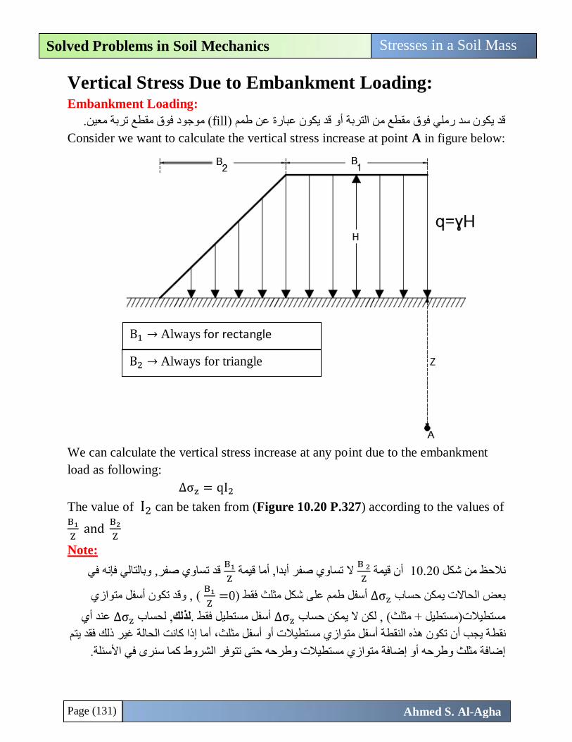
Page (131)
Stresses in a Soil Mass Solved Problems in Soil Mechanics
Ahmed S. Al-Agha
Vertical Stress Due to Embankment Loading: Embankment Loading:
( موجود فوق مقطع تربة معين. fillقد يكون سد رملي فوق مقطع من التربة أو قد يكون عبارة عن طمم )
Consider we want to calculate the vertical stress increase at point A in figure below:
We can calculate the vertical stress increase at any point due to the embankment
load as following:
∆σz = qI2
The value of I2 can be taken from (Figure 10.20 P.327) according to the values of B1
Z and
B2
Z
Note:
أن قيمة 10.20شكل نالحظ من B 2
Zتساوي صفر أبدا, أما قيمة ال
B1
Zوبالتالي فإنه في ,قد تساوي صفر
)أسفل طمم على شكل مثلث فقط σz∆بعض الحاالت يمكن حساب B1
Z( , وقد تكون أسفل متوازي 0=
عند أي σz∆لحساب ,لذلكأسفل مستطيل فقط . σz∆مستطيالت)مستطيل + مثلث( , لكن ال يمكن حساب
ة يجب أن تكون هذه النقطة أسفل متوازي مستطيالت أو أسفل مثلث، أما إذا كانت الحالة غير ذلك فقد يتم نقط
كما سنرى في األسئلة. إضافة مثلث وطرحه أو إضافة متوازي مستطيالت وطرحه حتى تتوفر الشروط
B1 → Always for rectangle
B2 → Always for triangle
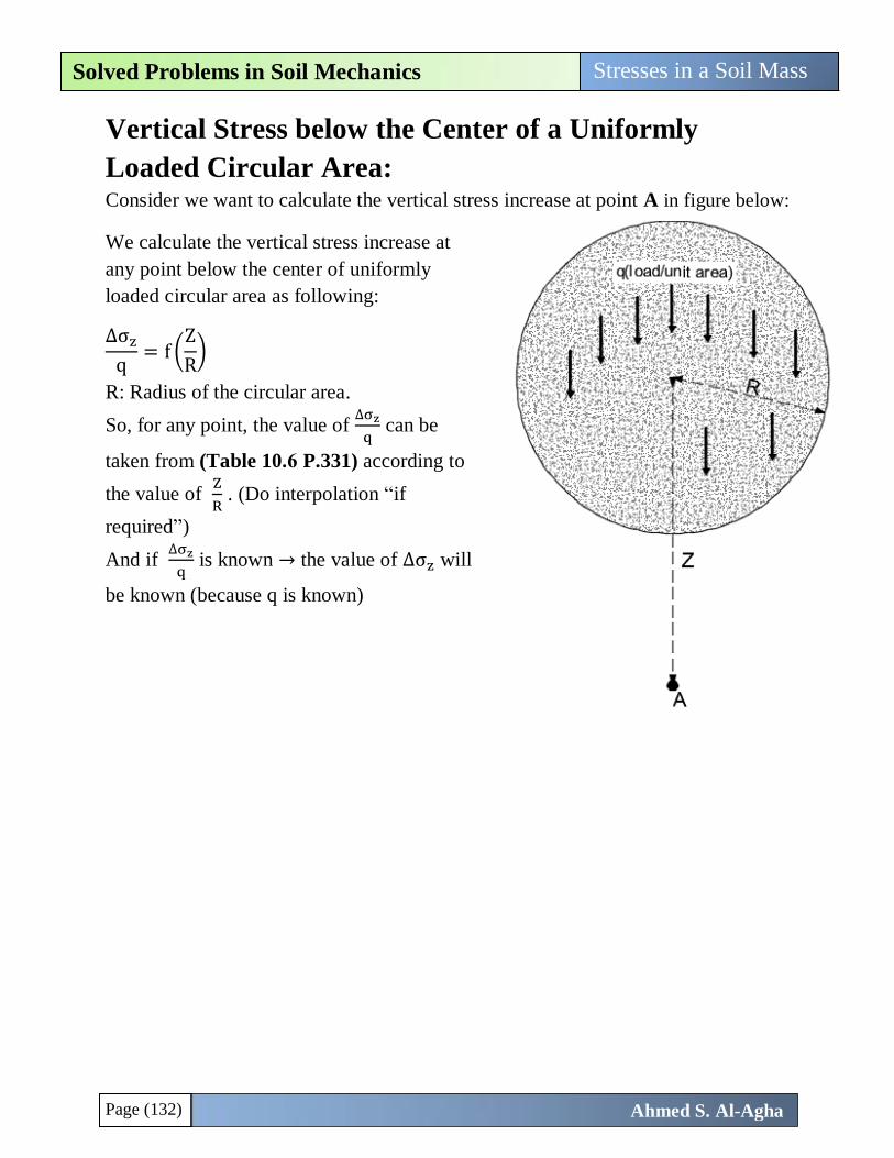
Page (132)
Stresses in a Soil Mass Solved Problems in Soil Mechanics
Ahmed S. Al-Agha
Vertical Stress below the Center of a Uniformly
Loaded Circular Area: Consider we want to calculate the vertical stress increase at point A in figure below:
We calculate the vertical stress increase at
any point below the center of uniformly
loaded circular area as following:
∆σz
q= f (
Z
R)
R: Radius of the circular area.
So, for any point, the value of ∆σz
q can be
taken from (Table 10.6 P.331) according to
the value of Z
R . (Do interpolation “if
required”)
And if ∆σz
q is known → the value of ∆σz will
be known (because q is known)
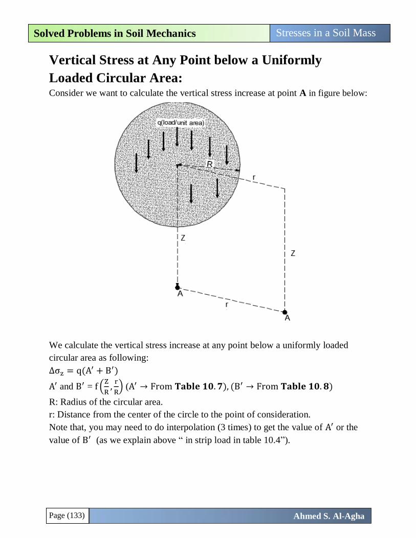
Page (133)
Stresses in a Soil Mass Solved Problems in Soil Mechanics
Ahmed S. Al-Agha
Vertical Stress at Any Point below a Uniformly
Loaded Circular Area: Consider we want to calculate the vertical stress increase at point A in figure below:
We calculate the vertical stress increase at any point below a uniformly loaded
circular area as following:
∆σz = q(A′ + B′)
A′ and B′ = f (Z
R,
r
R) (A′ → From 𝐓𝐚𝐛𝐥𝐞 𝟏𝟎. 𝟕), (B′ → From 𝐓𝐚𝐛𝐥𝐞 𝟏𝟎. 𝟖)
R: Radius of the circular area.
r: Distance from the center of the circle to the point of consideration.
Note that, you may need to do interpolation (3 times) to get the value of A′ or the
value of B′ (as we explain above “ in strip load in table 10.4”).
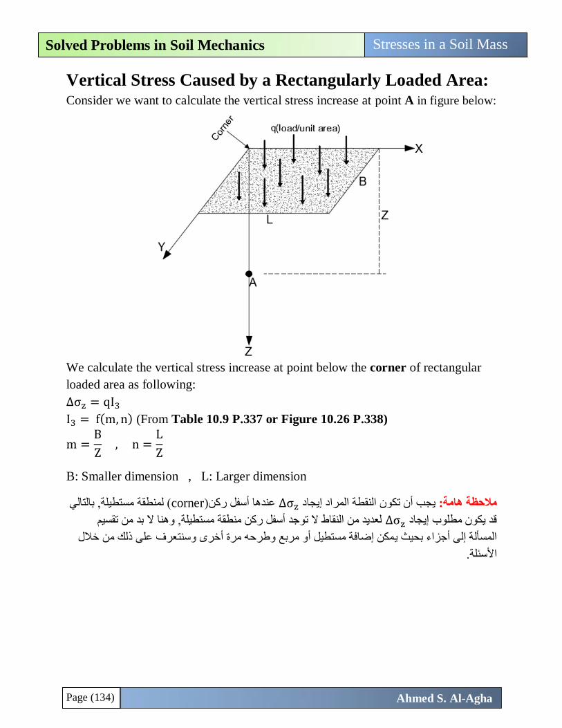
Page (134)
Stresses in a Soil Mass Solved Problems in Soil Mechanics
Ahmed S. Al-Agha
Vertical Stress Caused by a Rectangularly Loaded Area: Consider we want to calculate the vertical stress increase at point A in figure below:
We calculate the vertical stress increase at point below the corner of rectangular
loaded area as following:
∆σz = qI3
I3 = f(m, n) (From Table 10.9 P.337 or Figure 10.26 P.338)
m =B
Z , n =
L
Z
B: Smaller dimension , L: Larger dimension
( لمنطقة مستطيلة, بالتالي cornerعندها أسفل ركن) σz∆يجب أن تكون النقطة المراد إيجاد مالحظة هامة:
لعديد من النقاط ال توجد أسفل ركن منطقة مستطيلة, وهنا ال بد من تقسيم σz∆قد يكون مطلوب إيجاد
مكن إضافة مستطيل أو مربع وطرحه مرة أخرى وسنتعرف على ذلك من خالل بحيث يالمسألة إلى أجزاء
األسئلة.
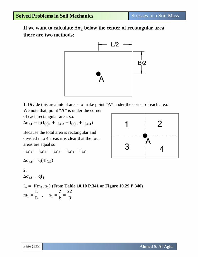
Page (135)
Stresses in a Soil Mass Solved Problems in Soil Mechanics
Ahmed S. Al-Agha
If we want to calculate ∆𝛔𝐳 below the center of rectangular area
there are two methods:
1. Divide this area into 4 areas to make point “A” under the corner of each area:
We note that, point “A” is under the corner
of each rectangular area, so:
∆σz,t = q(I(3)1 + I(3)2 + I(3)3 + I(3)4)
Because the total area is rectangular and
divided into 4 areas it is clear that the four
areas are equal so:
I(3)1 = I(3)2 = I(3)3 = I(3)4 = I(3)
∆σz,t = q(4I(3))
2.
∆σz,t = qI4
I4 = f(m1, n1) (From Table 10.10 P.341 or Figure 10.29 P.340)
m1 =L
B , n1 =
Z
b=
2Z
B
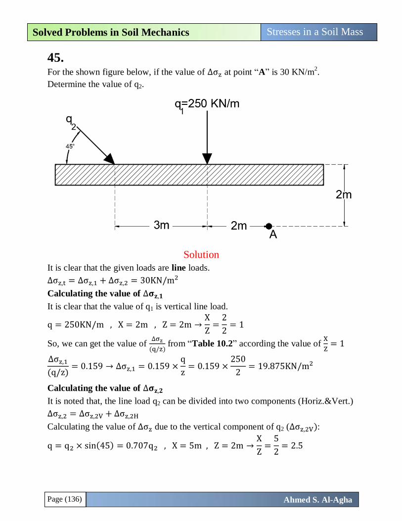
Page (136)
Stresses in a Soil Mass Solved Problems in Soil Mechanics
Ahmed S. Al-Agha
45. For the shown figure below, if the value of ∆σz at point “A” is 30 KN/m
2.
Determine the value of q2.
Solution
It is clear that the given loads are line loads.
∆σz,t = ∆σz,1 + ∆σz,2 = 30KN/m2
Calculating the value of ∆𝛔𝐳,𝟏
It is clear that the value of q1 is vertical line load.
q = 250KN/m , X = 2m , Z = 2m →X
Z=
2
2= 1
So, we can get the value of ∆σz
(q/z) from “Table 10.2” according the value of
X
Z= 1
∆σz,1
(q/z)= 0.159 → ∆σz,1 = 0.159 ×
q
z= 0.159 ×
250
2= 19.875KN/m2
Calculating the value of ∆𝛔𝐳,𝟐
It is noted that, the line load q2 can be divided into two components (Horiz.&Vert.)
∆σz,2 = ∆σz,2V + ∆σz,2H
Calculating the value of ∆σz due to the vertical component of q2 (∆σz,2V):
q = q2 × sin(45) = 0.707q2 , X = 5m , Z = 2m →X
Z=
5
2= 2.5
Page (137)
Stresses in a Soil Mass Solved Problems in Soil Mechanics
Ahmed S. Al-Agha
So, we can get the value of ∆σz
(q/z) from “Table 10.2” according the value of
X
Z= 2.5
∆σz,2V
(q/z)=
0.011 + 0.014
2= 0.0125 (average value between 2.4 and 2.6)
∆σz,2V = 0.0125 ×q
Z= 0.0125 ×
0.707q2
2= 4.419 × 10⁻³q2
Calculating the value of ∆σz due to the horizontal component of q2 (∆σz,2H):
q = q2 × cos(45) = 0.707q2 , X = 5m , Z = 2m →X
Z=
5
2= 2.5
So, we can get the value of ∆σz
(q/z) from “Table 10.3” according the value of
X
Z= 2.5
∆σz,2H
(q/z)=
0.051 + 0.019
2= 0.035 (average value between 2 and 3)
∆σz,2H = 0.035 ×q
Z= 0.035 ×
0.707q2
2= 0.01237q2
So, the total value of ∆σz,2 will be:
∆σz,2 = 4.419 × 10⁻³q2 + 0.01237q2 = 0.01679q2
∆σz,t = ∆σz,1 + ∆σz,2 = 30 KN/m2
30 = 19.875 + 0.01679q2 → q2 = 603KN/m ✓.
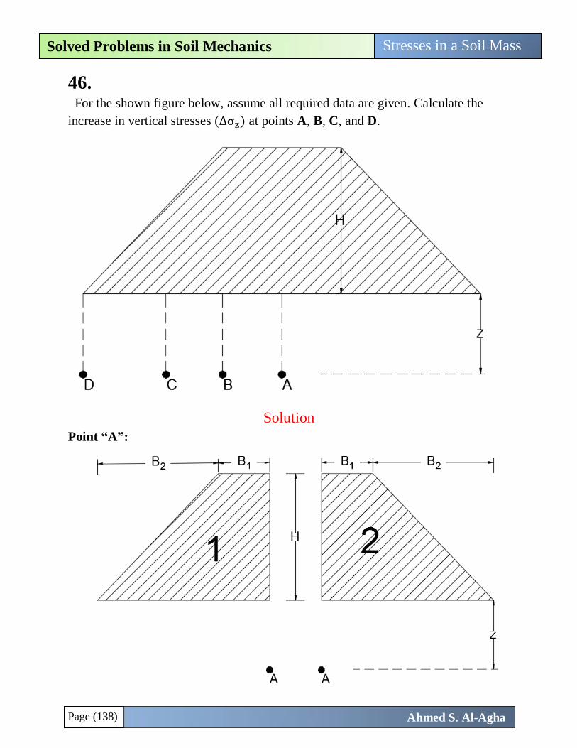
Page (138)
Stresses in a Soil Mass Solved Problems in Soil Mechanics
Ahmed S. Al-Agha
46. For the shown figure below, assume all required data are given. Calculate the
increase in vertical stresses (∆σz) at points A, B, C, and D.
Solution
Point “A”:
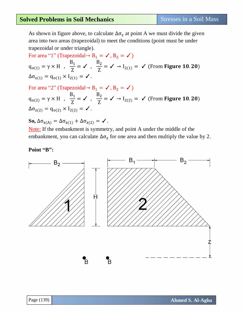
Page (139)
Stresses in a Soil Mass Solved Problems in Soil Mechanics
Ahmed S. Al-Agha
As shown in figure above, to calculate ∆σz at point A we must divide the given
area into two areas (trapezoidal) to meet the conditions (point must be under
trapezoidal or under triangle).
For area “1” (Trapezoidal→ B1 = ✓, B2 = ✓)
qo(1) = γ × H , B1
Z= ✓ ,
B2
Z= ✓ → I2(1) = ✓ (From 𝐅𝐢𝐠𝐮𝐫𝐞 𝟏𝟎. 𝟐𝟎)
∆σz(1) = qo(1) × I2(1) = ✓.
For area “2” (Trapezoidal→ B1 = ✓, B2 = ✓)
qo(2) = γ × H , B1
Z= ✓ ,
B2
Z= ✓ → I2(2) = ✓ (From 𝐅𝐢𝐠𝐮𝐫𝐞 𝟏𝟎. 𝟐𝟎)
∆σz(2) = qo(2) × I2(2) = ✓.
So, ∆σz(A) = ∆σz(1) + ∆σz(2) = ✓.
Note: If the embankment is symmetry, and point A under the middle of the
embankment, you can calculate ∆σz for one area and then multiply the value by 2.
Point “B”:
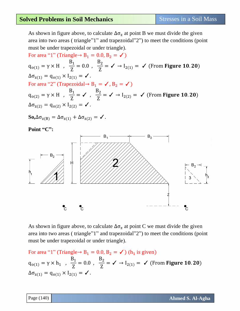
Page (140)
Stresses in a Soil Mass Solved Problems in Soil Mechanics
Ahmed S. Al-Agha
As shown in figure above, to calculate ∆σz at point B we must divide the given
area into two areas ( triangle”1” and trapezoidal”2”) to meet the conditions (point
must be under trapezoidal or under triangle).
For area “1” (Triangle→ B1 = 0.0, B2 = ✓)
qo(1) = γ × H , B1
Z= 0.0 ,
B2
Z= ✓ → I2(1) = ✓ (From 𝐅𝐢𝐠𝐮𝐫𝐞 𝟏𝟎. 𝟐𝟎)
∆σz(1) = qo(1) × I2(1) = ✓.
For area “2” (Trapezoidal→ B1 = ✓, B2 = ✓)
qo(2) = γ × H , B1
Z= ✓ ,
B2
Z= ✓ → I2(2) = ✓ (From 𝐅𝐢𝐠𝐮𝐫𝐞 𝟏𝟎. 𝟐𝟎)
∆σz(2) = qo(2) × I2(2) = ✓.
So,∆σz(B) = ∆σz(1) + ∆σz(2) = ✓.
Point “C”:
As shown in figure above, to calculate ∆σz at point C we must divide the given
area into two areas ( triangle”1” and trapezoidal”2”) to meet the conditions (point
must be under trapezoidal or under triangle).
For area “1” (Triangle→ B1 = 0.0, B2 = ✓) (h1 is given)
qo(1) = γ × h1 , B1
Z= 0.0 ,
B2
Z= ✓ → I2(1) = ✓ (From 𝐅𝐢𝐠𝐮𝐫𝐞 𝟏𝟎. 𝟐𝟎)
∆σz(1) = qo(1) × I2(1) = ✓.
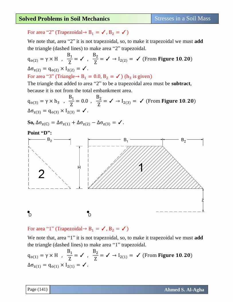
Page (141)
Stresses in a Soil Mass Solved Problems in Soil Mechanics
Ahmed S. Al-Agha
For area “2” (Trapezoidal→ B1 = ✓, B2 = ✓)
We note that, area “2” it is not trapezoidal, so, to make it trapezoidal we must add
the triangle (dashed lines) to make area “2” trapezoidal.
qo(2) = γ × H , B1
Z= ✓ ,
B2
Z= ✓ → I2(2) = ✓ (From 𝐅𝐢𝐠𝐮𝐫𝐞 𝟏𝟎. 𝟐𝟎)
∆σz(2) = qo(2) × I2(2) = ✓.
For area “3” (Triangle→ B1 = 0.0, B2 = ✓) (h3 is given)
The triangle that added to area “2” to be a trapezoidal area must be subtract,
because it is not from the total embankment area.
qo(3) = γ × h3 , B1
Z= 0.0 ,
B2
Z= ✓ → I2(3) = ✓ (From 𝐅𝐢𝐠𝐮𝐫𝐞 𝟏𝟎. 𝟐𝟎)
∆σz(3) = qo(3) × I2(3) = ✓.
So, ∆σz(C) = ∆σz(1) + ∆σz(2) − ∆σz(3) = ✓.
Point “D”:
For area “1” (Trapezoidal→ B1 = ✓, B2 = ✓)
We note that, area “1” it is not trapezoidal, so, to make it trapezoidal we must add
the triangle (dashed lines) to make area “1” trapezoidal.
qo(1) = γ × H , B1
Z= ✓ ,
B2
Z= ✓ → I2(1) = ✓ (From 𝐅𝐢𝐠𝐮𝐫𝐞 𝟏𝟎. 𝟐𝟎)
∆σz(1) = qo(1) × I2(1) = ✓.
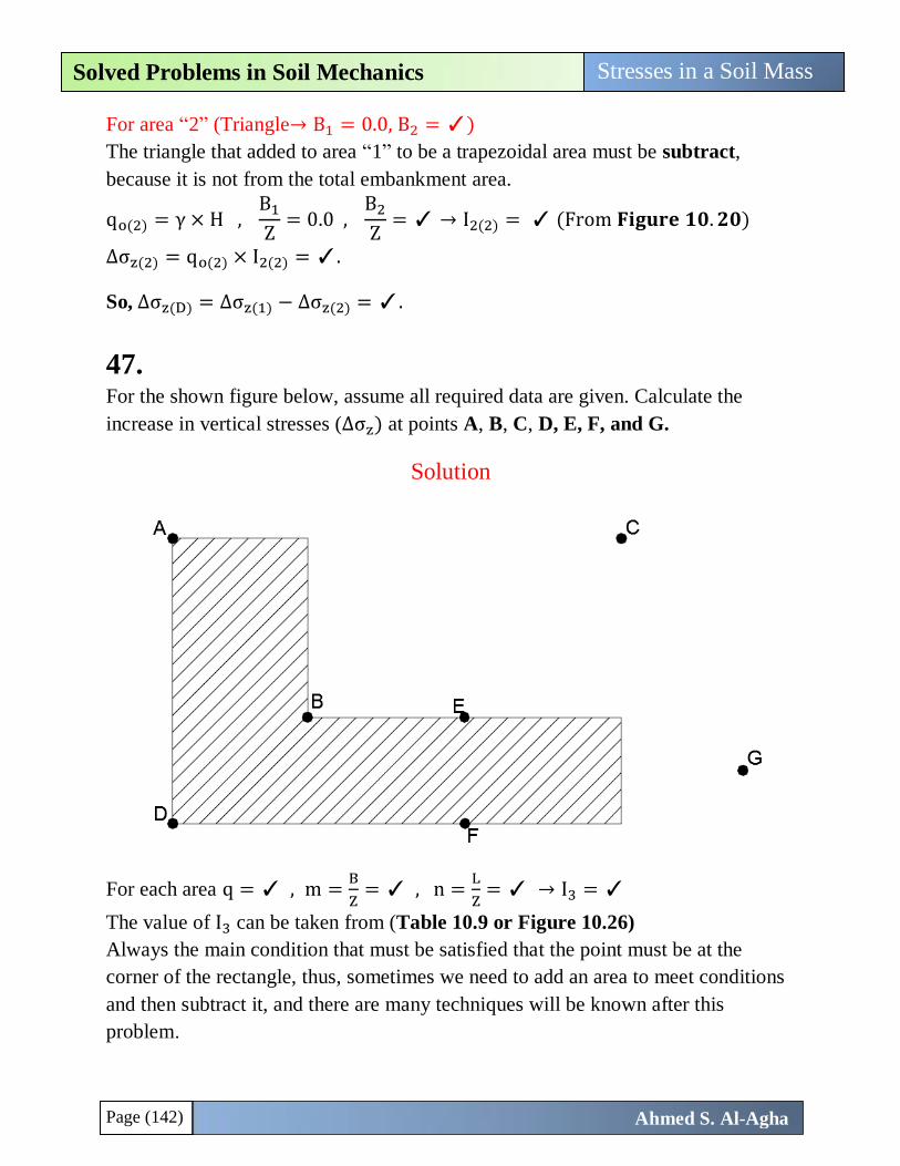
Page (142)
Stresses in a Soil Mass Solved Problems in Soil Mechanics
Ahmed S. Al-Agha
For area “2” (Triangle→ B1 = 0.0, B2 = ✓)
The triangle that added to area “1” to be a trapezoidal area must be subtract,
because it is not from the total embankment area.
qo(2) = γ × H , B1
Z= 0.0 ,
B2
Z= ✓ → I2(2) = ✓ (From 𝐅𝐢𝐠𝐮𝐫𝐞 𝟏𝟎. 𝟐𝟎)
∆σz(2) = qo(2) × I2(2) = ✓.
So, ∆σz(D) = ∆σz(1) − ∆σz(2) = ✓.
47.
For the shown figure below, assume all required data are given. Calculate the
increase in vertical stresses (∆σz) at points A, B, C, D, E, F, and G.
Solution
For each area q = ✓ , m =B
Z= ✓ , n =
L
Z= ✓ → I3 = ✓
The value of I3 can be taken from (Table 10.9 or Figure 10.26)
Always the main condition that must be satisfied that the point must be at the
corner of the rectangle, thus, sometimes we need to add an area to meet conditions
and then subtract it, and there are many techniques will be known after this
problem.
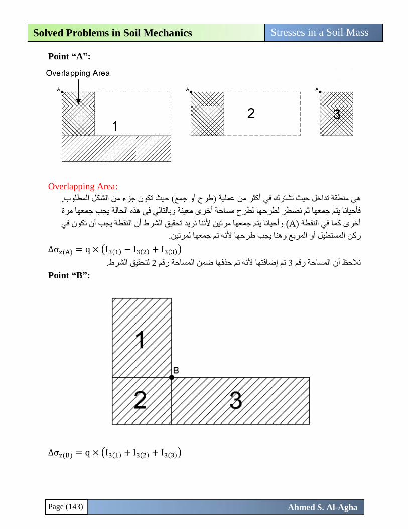
Page (143)
Stresses in a Soil Mass Solved Problems in Soil Mechanics
Ahmed S. Al-Agha
Point “A”:
Overlapping Area:
أكثر من عملية )طرح أو جمع( حيث تكون جزء من الشكل المطلوب, هي منطقة تداخل حيث تشترك في
لطرح مساحة أخرى معينة وبالتالي في هذه الحالة يجب جمعها مرة فأحيانا يتم جمعها ثم نضطر لطرحها
وأحيانا يتم جمعها مرتين ألننا نريد تحقيق الشرط أن النقطة يجب أن تكون في A))أخرى كما في النقطة
ل أو المربع وهنا يجب طرحها ألنه تم جمعها لمرتين.ركن المستطي
∆σz(A) = q × (I3(1) − I3(2) + I3(3))
لتحقيق الشرط. 2تم إضافتها ألنه تم حذفها ضمن المساحة رقم 3نالحظ أن المساحة رقم
Point “B”:
∆σz(B) = q × (I3(1) + I3(2) + I3(3))
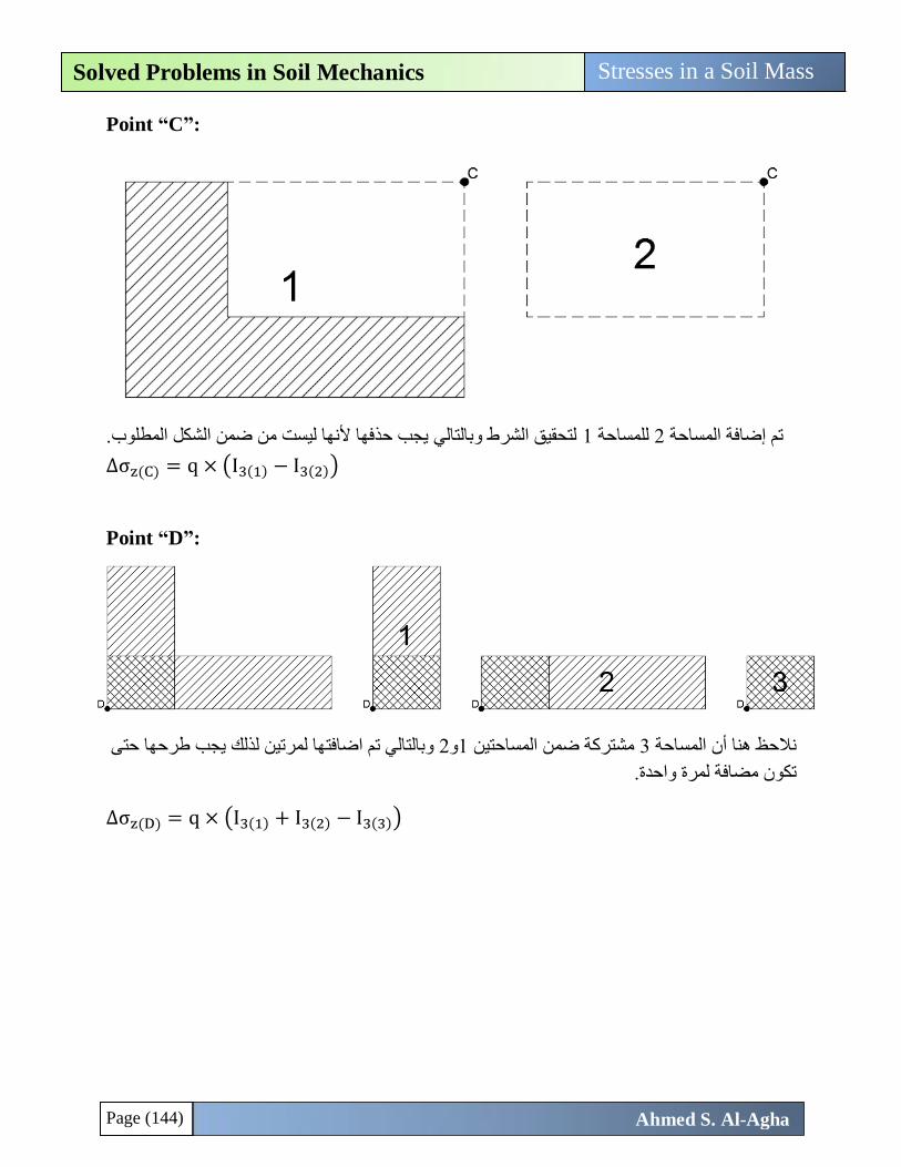
Page (144)
Stresses in a Soil Mass Solved Problems in Soil Mechanics
Ahmed S. Al-Agha
Point “C”:
لتحقيق الشرط وبالتالي يجب حذفها ألنها ليست من ضمن الشكل المطلوب. 1للمساحة 2ساحة تم إضافة الم
∆σz(C) = q × (I3(1) − I3(2))
Point “D”:
يجب طرحها حتى لذلكوبالتالي تم اضافتها لمرتين 2و1مشتركة ضمن المساحتين 3نالحظ هنا أن المساحة
تكون مضافة لمرة واحدة.
∆σz(D) = q × (I3(1) + I3(2) − I3(3))
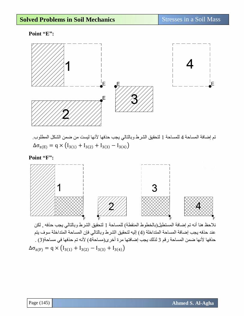
Page (145)
Stresses in a Soil Mass Solved Problems in Soil Mechanics
Ahmed S. Al-Agha
Point “E”:
لتحقيق الشرط وبالتالي يجب حذفها ألنها ليست من ضمن الشكل المطلوب. 1للمساحة 4تم إضافة المساحة
∆σz(E) = q × (I3(1) + I3(2) + I3(3) − I3(4))
Point “F”:
لتحقيق الشرط وبالتالي يجب حذفه , لكن 1للمساحة أنه تم إضافة المستطيل)بالخطوط المنقطة(نالحظ هنا
( إليه لتحقيق الشرط وبالتالي فإن المساحة المتداخلة سوف يتم 4عند حذفه يجب إضافة المساحة المتداخلة )
( .3( ألنه تم حذفها في مساحة)4يجب إضافتها مرة أخرى)مساحةلذلك 3حذفها ألنها ضمن المساحة رقم
∆σz(F) = q × (I3(1) + I3(2) − I3(3) + I3(4))
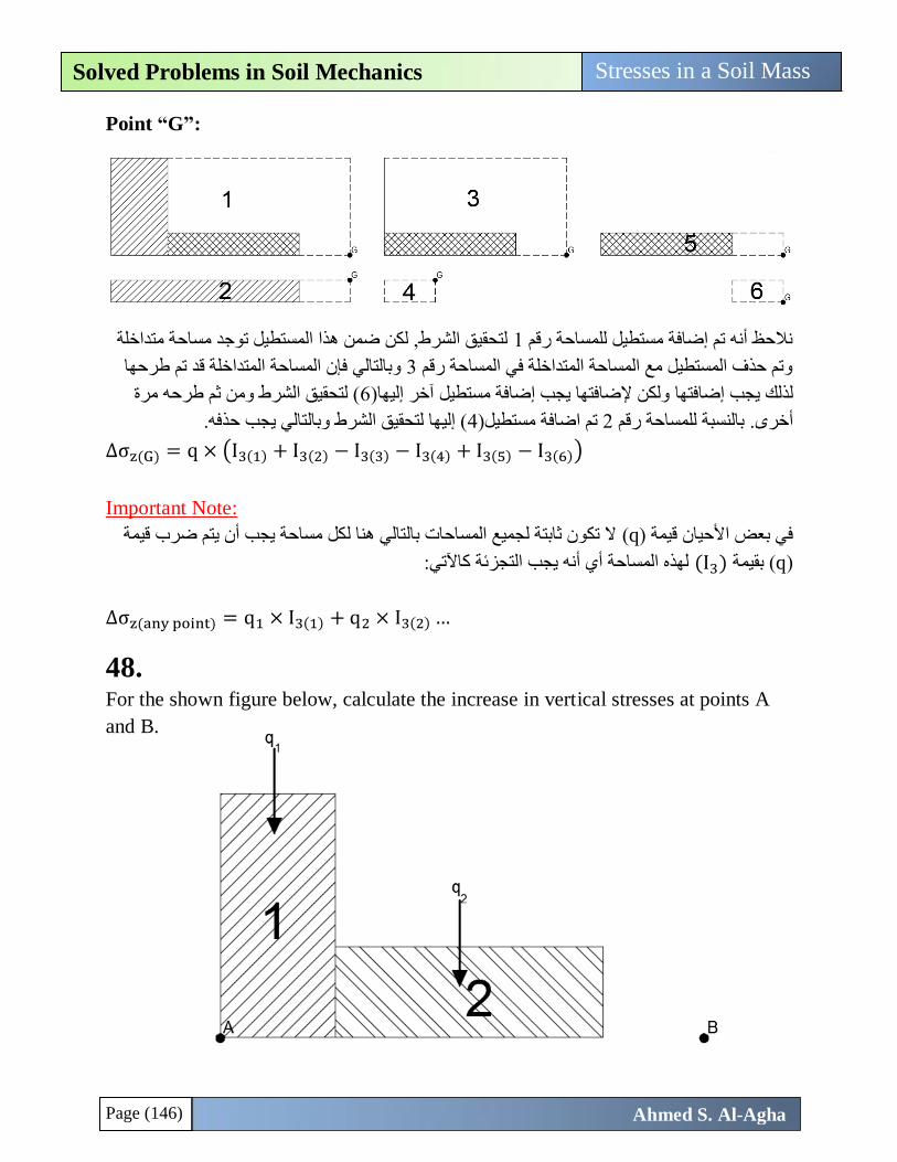
Page (146)
Stresses in a Soil Mass Solved Problems in Soil Mechanics
Ahmed S. Al-Agha
Point “G”:
لتحقيق الشرط, لكن ضمن هذا المستطيل توجد مساحة متداخلة 1نالحظ أنه تم إضافة مستطيل للمساحة رقم
وبالتالي فإن المساحة المتداخلة قد تم طرحها 3وتم حذف المستطيل مع المساحة المتداخلة في المساحة رقم
( لتحقيق الشرط ومن ثم طرحه مرة 6ولكن إلضافتها يجب إضافة مستطيل آخر إليها) يجب إضافتها لذلك
( إليها لتحقيق الشرط وبالتالي يجب حذفه.4تم اضافة مستطيل) 2بالنسبة للمساحة رقم رى.خأ
∆σz(G) = q × (I3(1) + I3(2) − I3(3) − I3(4) + I3(5) − I3(6))
Important Note:
ال تكون ثابتة لجميع المساحات بالتالي هنا لكل مساحة يجب أن يتم ضرب قيمة (q)ان قيمة في بعض األحي
(q) بقيمة(I3) :لهذه المساحة أي أنه يجب التجزئة كاآلتي
∆σz(any point) = q1 × I3(1) + q2 × I3(2) …
48.
For the shown figure below, calculate the increase in vertical stresses at points A
and B.
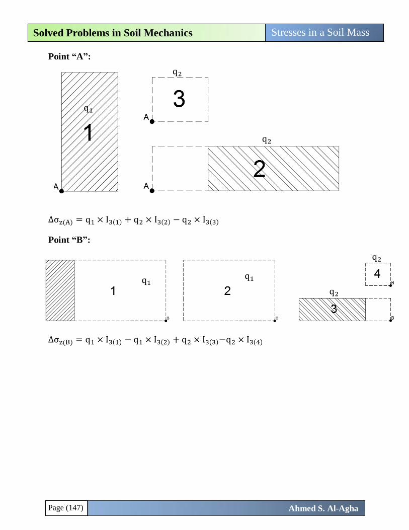
Page (147)
Stresses in a Soil Mass Solved Problems in Soil Mechanics
Ahmed S. Al-Agha
Point “A”:
∆σz(A) = q1 × I3(1) + q2 × I3(2) − q2 × I3(3)
Point “B”:
∆σz(B) = q1 × I3(1) − q1 × I3(2) + q2 × I3(3)−q2 × I3(4)
q1 q1
q2
q2
q1
q2
q2
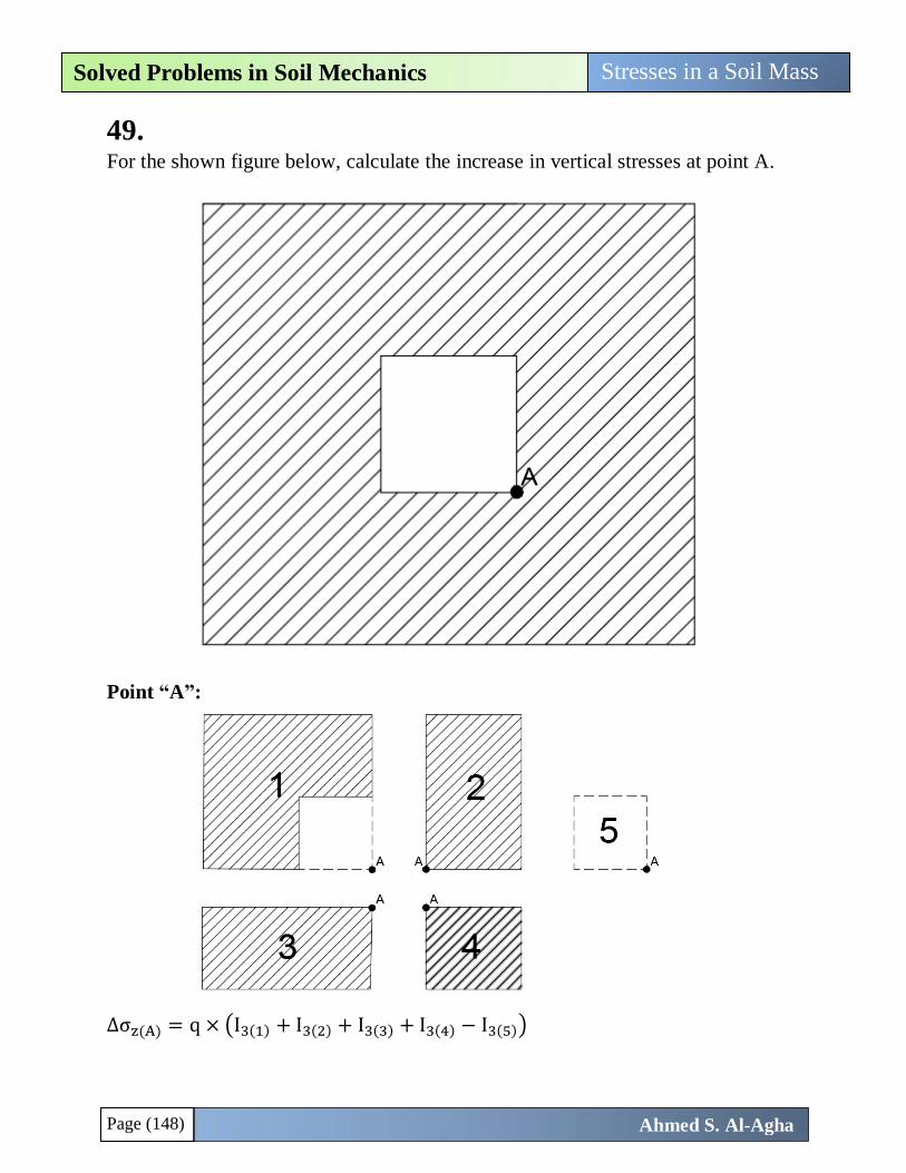
Page (148)
Stresses in a Soil Mass Solved Problems in Soil Mechanics
Ahmed S. Al-Agha
49.
For the shown figure below, calculate the increase in vertical stresses at point A.
Point “A”:
∆σz(A) = q × (I3(1) + I3(2) + I3(3) + I3(4) − I3(5))
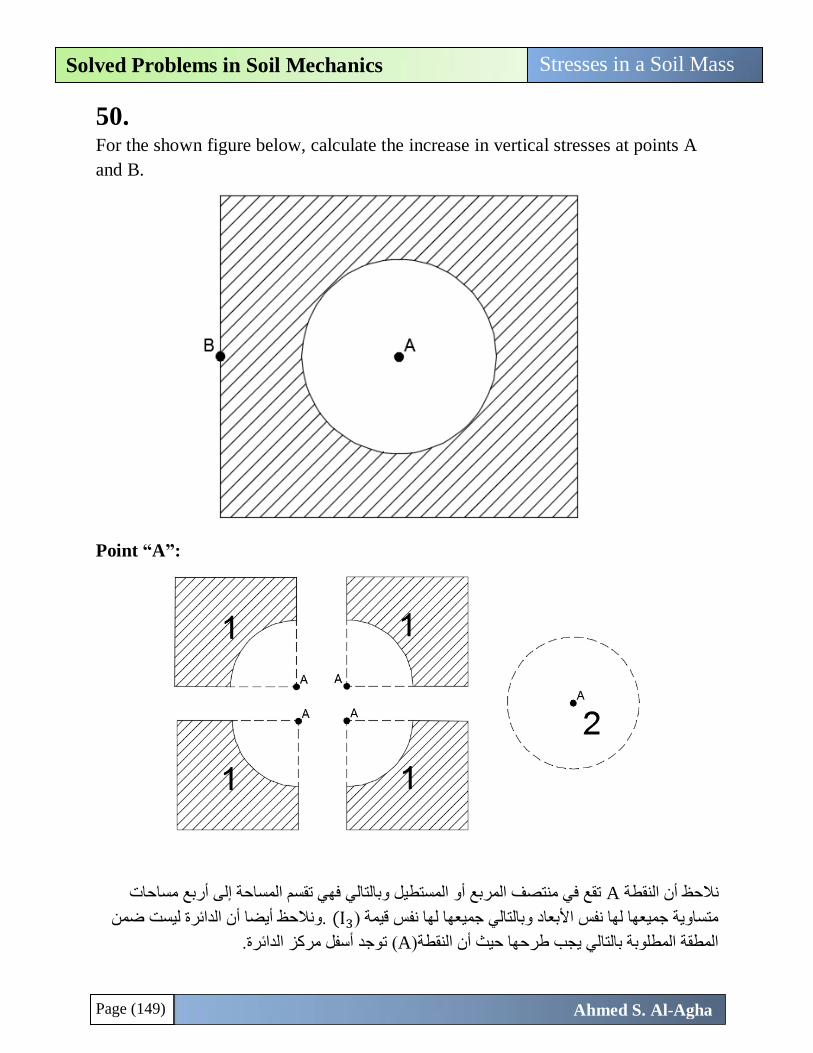
Page (149)
Stresses in a Soil Mass Solved Problems in Soil Mechanics
Ahmed S. Al-Agha
50.
For the shown figure below, calculate the increase in vertical stresses at points A
and B.
Point “A”:
تقع في منتصف المربع أو المستطيل وبالتالي فهي تقسم المساحة إلى أربع مساحات Aنالحظ أن النقطة
.ونالحظ أيضا أن الدائرة ليست ضمن I3))متساوية جميعها لها نفس األبعاد وبالتالي جميعها لها نفس قيمة
توجد أسفل مركز الدائرة.( A)المطقة المطلوبة بالتالي يجب طرحها حيث أن النقطة
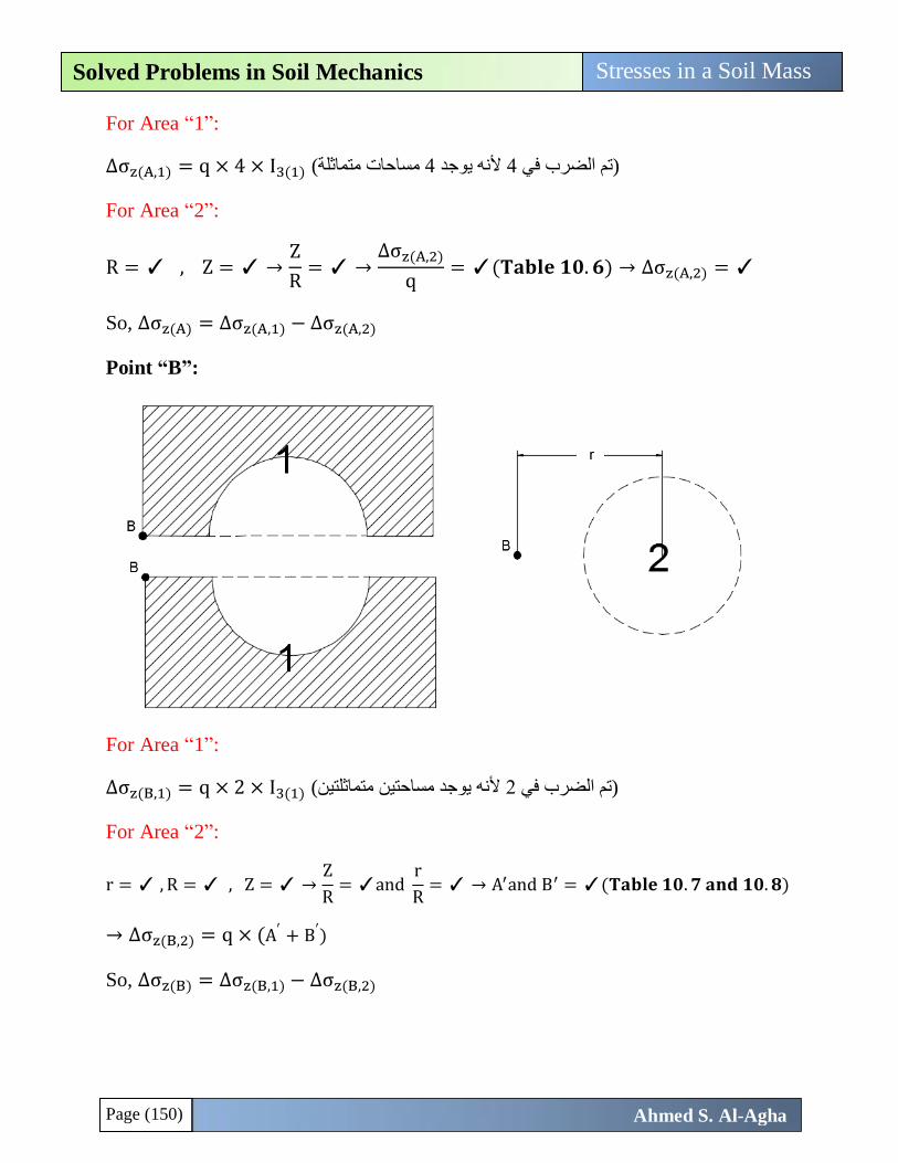
Page (150)
Stresses in a Soil Mass Solved Problems in Soil Mechanics
Ahmed S. Al-Agha
For Area “1”:
∆σz(A,1) = q × 4 × I3(1) ( مساحات متماثلة 4ألنه يوجد 4تم الضرب في )
For Area “2”:
R = ✓ , Z = ✓ →Z
R= ✓ →
∆σz(A,2)
q= ✓(𝐓𝐚𝐛𝐥𝐞 𝟏𝟎. 𝟔) → ∆σz(A,2) = ✓
So, ∆σz(A) = ∆σz(A,1) − ∆σz(A,2)
Point “B”:
For Area “1”:
∆σz(B,1) = q × 2 × I3(1) ( متماثلتين يوجد مساحتينألنه 2تم الضرب في )
For Area “2”:
r = ✓ , R = ✓ , Z = ✓ →Z
R= ✓and
r
R= ✓ → A′and B′ = ✓(𝐓𝐚𝐛𝐥𝐞 𝟏𝟎. 𝟕 𝐚𝐧𝐝 𝟏𝟎. 𝟖)
→ ∆σz(B,2) = q × (A′ + B′)
So, ∆σz(B) = ∆σz(B,1) − ∆σz(B,2)
Chapter (11)
Compressibility of Soil
Page (152)
Compressibility of Soil Solved Problems in Soil Mechanics
Ahmed S. Al-Agha
Introduction: إن وجود أحمال إضافية على التربة مثل حمل قاعدة أو حمل مبنى أو حمل سد رملي وغيره من األحمال
. هذا الهبوط له عدة أسباب (Settlementيؤدي إلى انضغاط حبيبات التربة وبالتالي يؤدي إلى هبوط التربة )
( خروج الماء والهواء من 3( إعادة تموضع حبيبات التربة, )2تشوه حبيبات التربة نتيجة األحمال, )( 1وهي)
.الفراغات الموجودة بين حبيبات التربة
In general, there are three basic types of settlement:
1. Elastic Settlement (Immediate Settlement):
حيث أنه يحدث أثناء وضع الهواء من الفراغات الموجودة في التربة هو الهبوط الذي يحدث نتيجة خروج
األحمال على التربة )بناية المنشأة( وينتهي بانتهاء وضع األحمال وال يحدث خالله أي تغير في نسبة
وهو )ألنه عبارة عن خروج الهواء فقط من بين حبيبات التربة(المحتوى المائي للطبقات المختلفة من التربة
.دث في جميع أنواع التربة سواء رمل أو طين وسواء كانت تربة جافة أو مشبعة بالماء أو مشبعة جزئيايح
2. Primary Consolidation Settlement:
ء من بين حبيبات التربة, وبالتالي ونتيجة لتطبيق هو الهبوط الذي يحدث في التربة نتيجة خروج الما
لذلك هذا النوع ,تتالشى وبالتالي سوف تهبط التربةلماء سوف األحمال فإن الفراغات التي يخرج منها ا
.من الهبوط يحدث في الطبقات المشبعة كليا بالماء
3. Secondary Consolidation Settlement:
يبدأ هذا النوع من primary consolidation))بعد خروج كل الماء من طبقة التربة وانتهاء مرحلة ال
الذي يحدث للتربة مع الزمن بسبب التشوه البالستيكيو ترتيب حبيبات التربةالهبوط والناتج عن إعادة
وتأثير األحمال.
So, the total settlement due to the applied load can be expressed as:
ST = Se + Sc + Ss
ST = Total Settlement
Se = Elastic Settlement (Immediate Settlemnt)
Sc = Primary Consolidation Settlement
Ss = Secondary Consolidation Settlement
In this chapter, the three types of settlement will be discussed completely.

Page (153)
Compressibility of Soil Solved Problems in Soil Mechanics
Ahmed S. Al-Agha
Elastic Settlement: As mentioned above, elastic or immediate settlement (Se) occurs directly after
the application of the load without change in the moisture content of the soil.
The magnitude of the elastic settlement will depend on the flexibility of the
foundation (flexible or rigid), and on the type of material (soil) that the
foundation will rest on it.
Elastic Settlement under a flexible foundation can be calculated from the
following equation:
Se = ∆σ(αB′)1 − μs
2
EsIsIf
L = Larger dimension of the foundation
B = Smaller dimension of the foundation
∆σ = Applied Net Pressure = Load/Area
μs = Poison′s Ratio
Es = Modulus of Elasticity
∆σ
Page (154)
Compressibility of Soil Solved Problems in Soil Mechanics
Ahmed S. Al-Agha
Es = Modulus of Elsticity of the soil through the depth H.
If there are more than one soil layer through the depth H we can find the modulus
of elasticity for all layers by weighted average method:
Es =∑ Es(i) × ∆Z
Z
Es(i) = Modulus of elasticity of each layer.
∆Z = Depth of each layer.
Z = H or 5B whichever is 𝐬𝐦𝐚𝐥𝐥𝐞𝐫
H = Distance from the face of the footing to the nearest rock layer (as shown in
figure above)
Now, as shown in figure above, the elastic settlement under a flexible foundation at
the center is larger than at the corner, thus, there are some different in calculating
(Se) under the center and under the corner of the footing.
This difference can be considered in the values of (B′ and α) .
For calculating 𝐒𝐞 under the center of the foundation:
B′ =B
2 and α = 4
For calculating 𝐒𝐞 under the corner of the foundation:
B′ = B and α = 1
Where, α = factor depends on the location on the foundation where settlement is
being calculated.
Is = shape factor.
Is = F1 +1−2μs
1−μsF2
F1(can be calculated from 𝐓𝐚𝐛𝐥𝐞 𝟏𝟏. 𝟏 𝐏. 𝟑𝟓𝟖)
F2(can be calculated from 𝐓𝐚𝐛𝐥𝐞 𝟏𝟏. 𝟐 𝐏. 𝟑𝟔𝟎)
To get the values of F1and (F2) from tables we need the values of m′and n′
m′ =L
B , n′ =
H
B′
If = factor depens on depth of excavation, footing dimensions and soil type
The value of (If) can be calculated from (Table 11.3 P.362).
Note: If Df = 0.0 →→ If = 1
Page (155)
Compressibility of Soil Solved Problems in Soil Mechanics
Ahmed S. Al-Agha
Elastic Settlement under a rigid foundation:
From the figure above (page 138) it is noted that the elastic settlement under a rigid
foundation is constant and less than Se for flexible foundation (at center).
So, the value of Se under a rigid foundation can be estimated as following:
Se(rigid) = 0.93Se(flexible,center)
See (example 11.1 P.362) in your textbook.
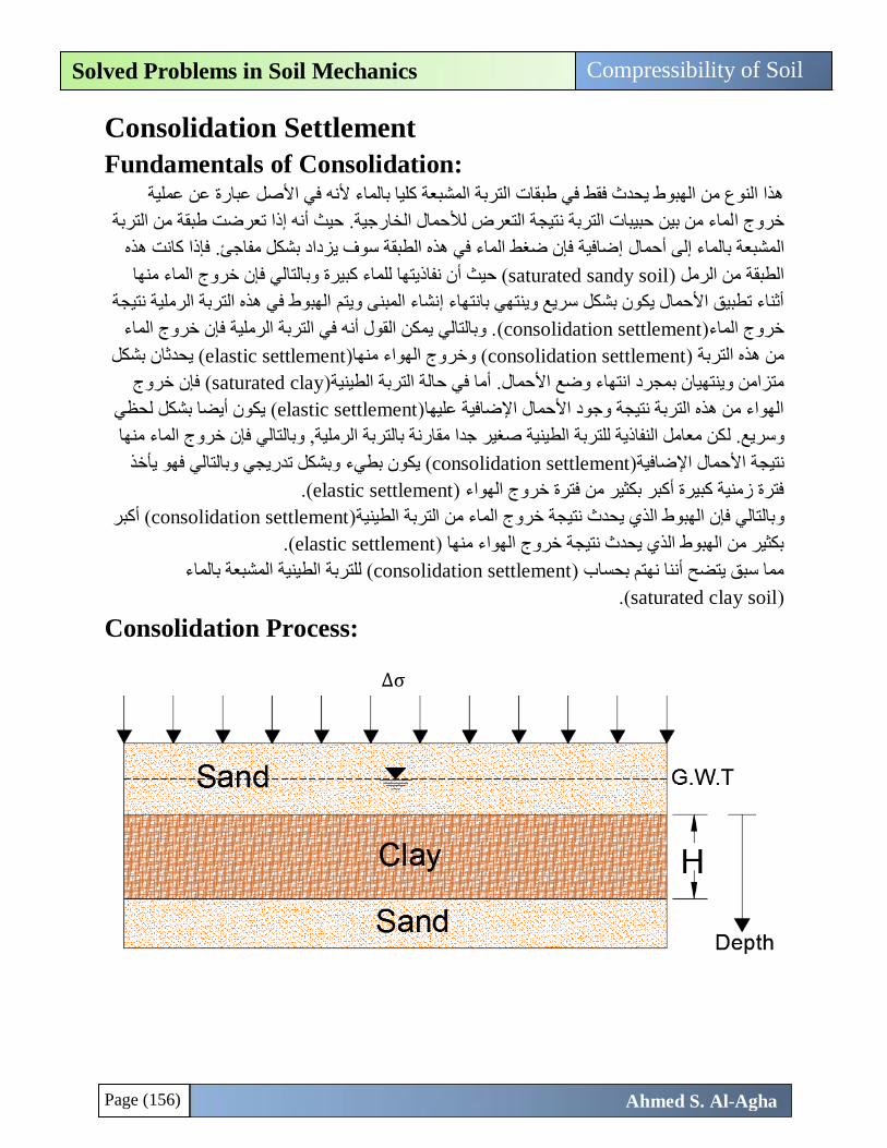
Page (156)
Compressibility of Soil Solved Problems in Soil Mechanics
Ahmed S. Al-Agha
Consolidation Settlement
Fundamentals of Consolidation: هذا النوع من الهبوط يحدث فقط في طبقات التربة المشبعة كليا بالماء ألنه في األصل عبارة عن عملية
حيث أنه إذا تعرضت طبقة من التربة لماء من بين حبيبات التربة نتيجة التعرض لألحمال الخارجية.خروج ا
فإذا كانت هذه إضافية فإن ضغط الماء في هذه الطبقة سوف يزداد بشكل مفاجئ. لمشبعة بالماء إلى أحماال
لتالي فإن خروج الماء منها وباللماء كبيرة ا( حيث أن نفاذيتهsaturated sandy soilالطبقة من الرمل )
الهبوط في هذه التربة الرملية نتيجة ويتم أثناء تطبيق األحمال يكون بشكل سريع وينتهي بانتهاء إنشاء المبنى
. وبالتالي يمكن القول أنه في التربة الرملية فإن خروج الماء (consolidation settlement)خروج الماء
( يحدثان بشكل elastic settlement( وخروج الهواء منها)consolidation settlementمن هذه التربة )
( فإن خروج saturated clayأما في حالة التربة الطينية) متزامن وينتهيان بمجرد انتهاء وضع األحمال.
يكون أيضا بشكل لحظي (elastic settlement)الهواء من هذه التربة نتيجة وجود األحمال اإلضافية عليها
فإن خروج الماء منها كن معامل النفاذية للتربة الطينية صغير جدا مقارنة بالتربة الرملية, وبالتالي ل .وسريع
وبشكل تدريجي وبالتالي فهو يأخذ يكون بطيء (consolidation settlement)نتيجة األحمال اإلضافية
.(elastic settlementفترة زمنية كبيرة أكبر بكثير من فترة خروج الهواء )
( أكبر consolidation settlementالطينية) بالتالي فإن الهبوط الذي يحدث نتيجة خروج الماء من التربةو
(.elastic settlementبكثير من الهبوط الذي يحدث نتيجة خروج الهواء منها )
( للتربة الطينية المشبعة بالماءconsolidation settlement) مما سبق يتضح أننا نهتم بحساب
(saturated clay soil.)
Consolidation Process:
∆σ
Page (157)
Compressibility of Soil Solved Problems in Soil Mechanics
Ahmed S. Al-Agha
( وهذا permeable sandمحصورة بين طبقتين من ال) clay))نالحظ من الشكل في األعلى أن طبقة ال
فإن المياه سوف تخرج من الطبقة عن طريق حركة المياه من منتصف (σ∆)تطبيق الحمل يعني أنه نتيجة
فإنه (σ∆)عند وضع الحمل اإلضافي ياه من منتصف الطبقة إلى أسفل.الطبقة إلى أعلى وأيضا حركة الم
(σ∆)سوف ينتقل إلى الماء الموجود داخل حبيبات التربة وإلى حبيبات التربة نفسها وهذا يعني أن قيمة
وبالتالي: .(Effective Stress and Pore Water Pressureسوف تنقسم إلى قسمين )
∆σ = ∆σ′ + ∆u
∆σ′ = increase in effective stress due to application of ∆σ
∆u = increase in pore water pressure due to application of ∆σ
or ∆u = excess in pore water pressure
So, if there exist an additional load (∆σ) , the total effective stress and the total
pore water pressure at any depth in the clay layer are:
σ′ = σo′ + ∆σ′
u = uo + ∆u
σo′ = present effective stress at any point due to the weight of soils above this point
(exactly as CH. 9)(also called present effective overburden pressure )
uo = pore water pressure due to the height of G.W.T above a certain point (as ch.9)
The values of (∆u) and (∆σ′) are varies with time during the consolidation process
as following:
قبل وضع أي أحمال على المنشأ, أي أنه ال يوجد أي أحمال إضافية فإنه ال توجد أي زيادة في كل من .1
غط الماء واإلجهاد الفعال وبالتالي:ض
Before applying any additional loading:
∆σ = 0.0 → ∆u =0.0 and ∆σ′ = 0.0 →→ σ′ = σo′ and u = uo
( σ∆( فإن كل قيمة الحمل اإلضافي)t = 0.0( مباشرة أي عند زمن )σ∆بعد وضع األحمال اإلضافية ) .2
زء منه تحمله التربة وهذا يرجع إلى أن التربة الطينية معامل النفاذية لها تنتقل إلى الماء وال يوجد أي جسوف
صغير جدا وبالتالي أثناء تطبيق الحمل مباشرة فإن الماء لم يبدأ بالخروج بعد من طبقة الطين وبالتالي فأن
( وبالتالي:σ∆الماء هو الذي يتحمل كل الحمل اإلضافي )
Just after (at t = 0.0) applying additional loading(∆σ):
∆u =∆σ and ∆σ′ = 0 →→ σ′ = σo′ and u = uo + ∆σ
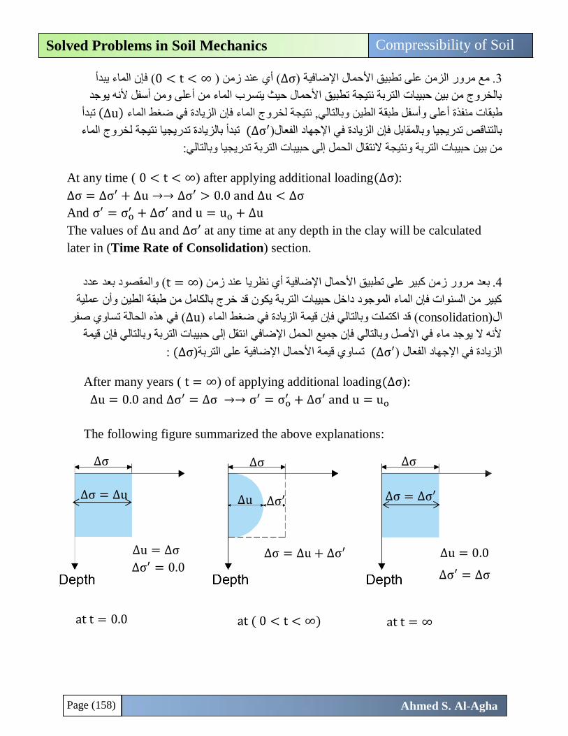
Page (158)
Compressibility of Soil Solved Problems in Soil Mechanics
Ahmed S. Al-Agha
0 ) ( أي عند زمنσ∆مع مرور الزمن على تطبيق األحمال اإلضافية ) .3 < t < ( فإن الماء يبدأ ∞
بالخروج من بين حبيبات التربة نتيجة تطبيق األحمال حيث يتسرب الماء من أعلى ومن أسفل ألنه يوجد
تبدأ (u∆) وبالتالي, نتيجة لخروج الماء فإن الزيادة في ضغط الماء ت منفذة أعلى وأسفل طبقة الطينطبقا
نتيجة لخروج الماء تبدأ بالزيادة تدريجيا ′σ∆) بالتناقص تدريجيا وبالمقابل فإن الزيادة في اإلجهاد الفعال)
بة تدريجيا وبالتالي:من بين حبيبات التربة ونتيجة النتقال الحمل إلى حبيبات التر
At any time ( 0 < t < ∞) after applying additional loading(∆σ):
∆σ = ∆σ′ + ∆u →→ ∆σ′ > 0.0 and ∆u < ∆σ
And σ′ = σo′ + ∆σ′ and u = uo + ∆u
The values of ∆u and ∆σ′ at any time at any depth in the clay will be calculated
later in (Time Rate of Consolidation) section.
t) مرور زمن كبير على تطبيق األحمال اإلضافية أي نظريا عند زمنبعد .4 = ( والمقصود بعد عدد ∞
وأن عملية كبير من السنوات فإن الماء الموجود داخل حبيبات التربة يكون قد خرج بالكامل من طبقة الطين
في هذه الحالة تساوي صفر ( u∆) ضغط الماءالزيادة في قيمة ( قد اكتملت وبالتالي فإن(consolidationال
ألنه ال يوجد ماء في األصل وبالتالي فإن جميع الحمل اإلضافي انتقل إلى حبيبات التربة وبالتالي فإن قيمة
: (σ∆)تساوي قيمة األحمال اإلضافية على التربة ′σ∆) )الزيادة في اإلجهاد الفعال
After many years ( t = ∞) of applying additional loading(∆σ):
∆u = 0.0 and ∆σ′ = ∆σ →→ σ′ = σo′ + ∆σ′ and u = uo
The following figure summarized the above explanations:
∆σ ∆σ ∆σ
∆u ∆σ′ ∆σ = ∆u ∆σ = ∆σ′
at t = 0.0
∆u = ∆σ
∆σ′ = 0.0
∆σ = ∆u + ∆σ′
at ( 0 < t < ∞)
at t = ∞
∆u = 0.0
∆σ′ = ∆σ
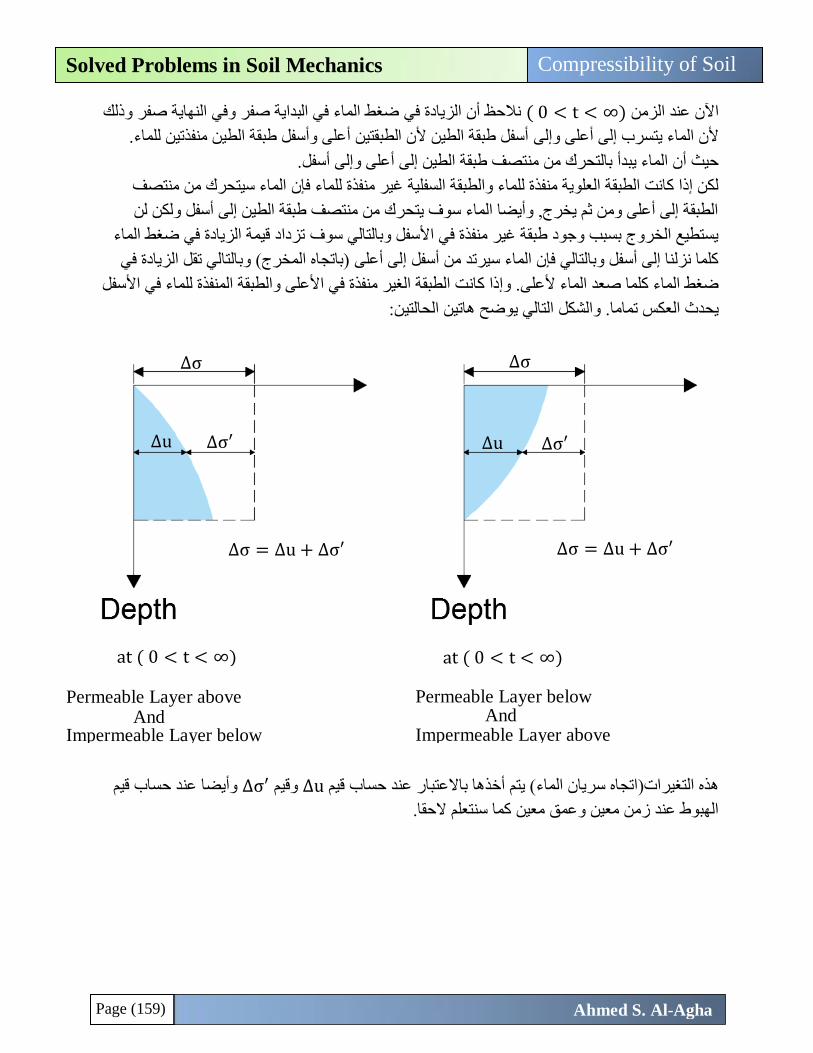
Page (159)
Compressibility of Soil Solved Problems in Soil Mechanics
Ahmed S. Al-Agha
0 )اآلن عند الزمن < t < النهاية صفر وذلك ضغط الماء في البداية صفر وفي الزيادة في نالحظ أن (∞
أسفل طبقة الطين ألن الطبقتين أعلى وأسفل طبقة الطين منفذتين للماء. إلىأعلى و إلىألن الماء يتسرب
تصف طبقة الطين إلى أعلى وإلى أسفل.نحيث أن الماء يبدأ بالتحرك من م
الماء سيتحرك من منتصف ير منفذة للماء فإن لكن إذا كانت الطبقة العلوية منفذة للماء والطبقة السفلية غ
الطبقة إلى أعلى ومن ثم يخرج, وأيضا الماء سوف يتحرك من منتصف طبقة الطين إلى أسفل ولكن لن
ضغط الماء تزداد قيمة الزيادة فييستطيع الخروج بسبب وجود طبقة غير منفذة في األسفل وبالتالي سوف
)باتجاه المخرج( وبالتالي تقل الزيادة في إلى أعلى كلما نزلنا إلى أسفل وبالتالي فإن الماء سيرتد من أسفل
ت الطبقة الغير منفذة في األعلى والطبقة المنفذة للماء في األسفل ضغط الماء كلما صعد الماء ألعلى. وإذا كان
التالي يوضح هاتين الحالتين: ليحدث العكس تماما. والشك
وأيضا عند حساب قيم ′σ∆وقيم u∆( يتم أخذها باالعتبار عند حساب قيم هذه التغيرات)اتجاه سريان الماء
.كما سنتعلم الحقاالهبوط عند زمن معين وعمق معين
∆σ ∆σ
∆u ∆σ′
∆σ = ∆u + ∆σ′
at ( 0 < t < ∞)
at ( 0 < t < ∞)
∆σ = ∆u + ∆σ′
∆u ∆σ′
Permeable Layer above
Impermeable Layer below
belowabove
Permeable Layer below
Impermeable Layer above
belowabove
And And
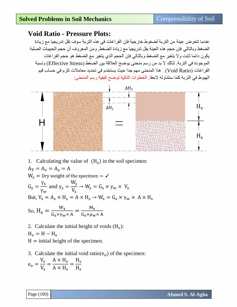
Page (160)
Compressibility of Soil Solved Problems in Soil Mechanics
Ahmed S. Al-Agha
Void Ratio - Pressure Plots: من التربة لضغوط خارجية فإن الفراغات في هذه التربة سوف تقل تدريجيا مع زيادة عندما تتعرض عينة
فإن حجم هذه العينة يقل تدريجيا مع زيادة الضغط, ومن المعروف أن حجم الحبيبات الصلبة الضغط وبالتالي
يكون دائما ثابت وال يتغير مع الضغط وبالتالي فإن الحجم الذي يتغير مع الضغط هو حجم الفراغات
( ونسبة Effective Stress) ال بد من رسم منحنى يوضح العالقة بين الضغط لذلك. الموجودة في التربة
في تحديد معامالت تلزم في حساب قيم يستخدمهذا المنحنى مهم جدا حيث .( Void Ratioالفراغات )
الخطوات التالية توضح كيفية رسم المنحنى:الهبوط في التربة كما سنتناوله الحقا.
1. Calculating the value of (Hs) in the soil specimen:
AT = Av = As = A
Ws = Dry weight of the specimen = ✓
Gs =γs
γw and γs =
Ws
Vs→ Ws = Gs × γw × Vs
But, Vs = As × Hs = A × Hs → Ws = Gs × γw × A × Hs
So, Hs =Ws
Gs×γw× A=
Ms
Gs×ρw× A
2. Calculate the initial height of voids (Hv):
Hv = H − Hs
H = initial height of the specimen.
3. Calculate the initial void ratio(eo) of the specimen:
eo =Vv
Vs=
A × Hv
A × Hs=
Hv
Hs
∆H1
∆H2
Hv
Hs
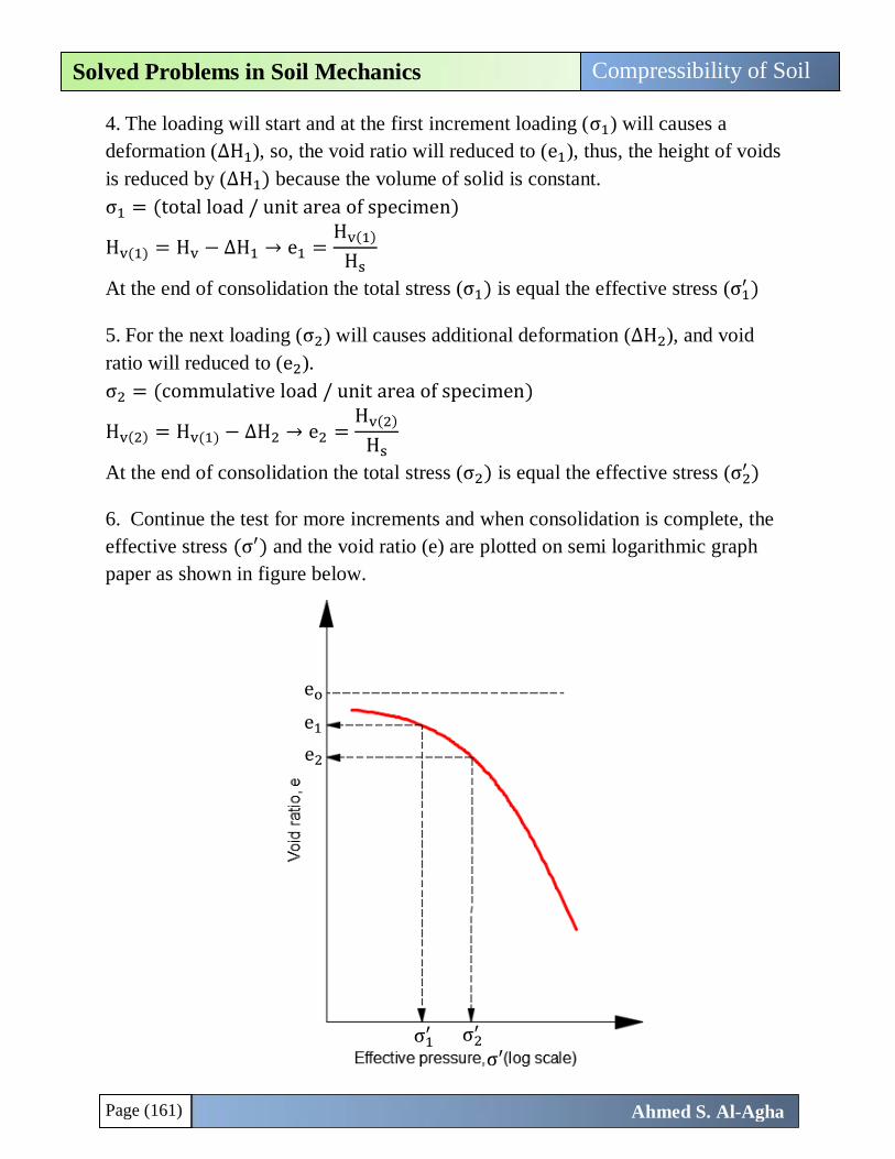
Page (161)
Compressibility of Soil Solved Problems in Soil Mechanics
Ahmed S. Al-Agha
4. The loading will start and at the first increment loading (σ1) will causes a
deformation (∆H1), so, the void ratio will reduced to (e1), thus, the height of voids
is reduced by (∆H1) because the volume of solid is constant.
σ1 = (total load / unit area of specimen)
Hv(1) = Hv − ∆H1 → e1 =Hv(1)
Hs
At the end of consolidation the total stress (σ1) is equal the effective stress (σ1′ )
5. For the next loading (σ2) will causes additional deformation (∆H2), and void
ratio will reduced to (e2).
σ2 = (commulative load / unit area of specimen)
Hv(2) = Hv(1) − ∆H2 → e2 =Hv(2)
Hs
At the end of consolidation the total stress (σ2) is equal the effective stress (σ2′ )
6. Continue the test for more increments and when consolidation is complete, the
effective stress (σ′) and the void ratio (e) are plotted on semi logarithmic graph
paper as shown in figure below.
σ′
σ1′ σ2
′
e1
e2
eo
Page (162)
Compressibility of Soil Solved Problems in Soil Mechanics
Ahmed S. Al-Agha
Normally Consolidated and Overconsolidated Clays: Normally Consolidated Clay: The present effective overburden pressure (σo
′ ) is
the maximum pressure that the soil was subjected to in the past (this means, the
soil has never subjected to a vertical effective overburden pressure greater than the
present effective vertical pressure)
ون عند إنشاء مبنى معين يتم وضع القواعد مباشرة على سطح األرض د مثال على هذا النوع من التربة:
حفر أي كمية من التربة وبالتالي فإن طبقة الطين الموجودة على عمق معين يكون عليها حمل كل التربة التي
فوقها وهو أقصى حمل ممكن أن تؤثره التربة على هذه الطبقة حيث يبدأ التحميل مباشرة من سطح األرض
الكبيرة فإن الهبوط يكون كبير نوعا أي أنه يتم وضع القواعد على سطح األرض مباشرة, وهنا نتيجة األحمال
ما.
Overconsolidated Clay: The present effective overburden pressure (σo′ ) is less
than the maximum effective overburden pressure that the soil was subjected to in
the past.
نى معين من المعروف أنه بدون حفر غالبا ما تكون قيمة عند إنشاء مب مثال على هذا النوع من التربة:
σo)اإلجهاد الفعال الحالي ′ هي أقصى قيمة تعرضت طبقة طين على بعد معين من التربة وهذه هي الحالة (
لكن إذا كان هناك مبنى وفيه طابق بدروم فإنه ال بد من الحفر داخل التربة إلى عمق األولى المذكورة أعاله.
σo)بالتالي فإن اإلجهاد الفعال الحاليمعين و′ الموجود على طبقة الطين والموجودة على عمق معين سوف (
وبالتالي نالحظ أنه حتى نصل إلى يكون أقل من قيمة أقصى إجهاد فعال تعرضت له في الماضي)قبل الحفر(
قليل األحمال على طبقة )أي ت كمية معينة من التربةقد تم حفر Overconsolidated Clay) )حالة ال
( ثم يتم وضع المنشأة وتطبيق األحمال وهذه العملية تسمى Unloadingالطين( وهذه العملية تسمى )
(Loading or Recompression نالحظ أيضا في هذا النوع من الطين تكون األحمال على طبقة الطين. )
. (Normally Consolidated Clay) قليلة نوعا ما وبالتالي تكون قيم الهبوط أقل منها في حالة
( . لكن لحساب قيم الهبوط التي تنتج عن كل نوع in fieldالكالم الموضح أعاله يبين ما يحدث في الموقع )
من التربة ال بد من تمثيل ما يحدث في الواقع في المختبر لحساب بعض المعامالت الهامة والتي تلزم في
وعي التربة في المختبر في تجربة واحدة كما يلي:حيث يتم تمثيل ن الهبوط.قيم حساب
حيث يكون الضغط في البداية يتم وضع عينة من الطين تحت ضغط معين ويبدأ عليها الضغط تدريجيا .1
تكون صغيرة في البداية وهذا يتمثل في ) ”e“)النقصان في قيمة صغير نوعا ما وبالتالي فإن قيم الهبوط
وهذه هي المرحلة األولى والتي تتمثل في بداية بناء المنشأة موجود في األسفلعلى المنحنى ال ”ab“المسافة
.)على سطح التربة بدون حفر(في الموقع
( تزاد بشكل ”e“قيم الهبوط )النقصان في قيمة الحمل بالزيادة تدريجيا على العينة وبالتالي فإن يبدأ .2
ى المنحنى المجود في األسفل حيث أن التربة في عل ”bc“مع زيادة األحمال وهذا يتمثل في المسافة ملحوظ
بفترة معينة ةوتتمثل في الموقع )بعد بداية تنفيذ المنشأ (normally consolidated clay)هذه الحالة تكون
ة ووضع كافة األحمال(.من تنفيذ المنشأ االنتهاءإلى
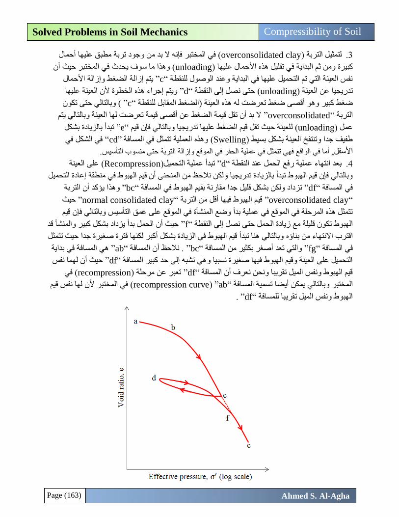
Page (163)
Compressibility of Soil Solved Problems in Soil Mechanics
Ahmed S. Al-Agha
ن وجود تربة مطبق عليها أحمال ( في المختبر فإنه ال بد مoverconsolidated clayلتمثيل التربة ) .3
( وهذا ما سوف يحدث في المختبر حيث أن unloadingومن ثم البداية في تقليل هذه األحمال عليها )كبيرة
يتم إزالة الضغط وإزالة األحمال ”c“نفس العينة التي تم التحميل عليها في البداية وعند الوصول للنقطة
ويتم إجراء هذه الخطوة ألن العينة عليها ”d“نصل إلى النقطة حتى (unloading) تدريجيا عن العينة
وبالتالي حتى تكون ( ”c“أقصى ضغط تعرضت له هذه العينة )الضغط المقابل للنقطة وضغط كبير وه
ال بد أن تقل قيمة الضغط عن أقصى قيمة تعرضت لها العينة وبالتالي يتم ”overconsolidated“التربة
تبدأ بالزيادة بشكل ”e“لعينة حيث تقل قيم الضغط عليها تدريجيا وبالتالي فإن قيم ( لunloadingعمل )
في الشكل في ”cd“وهذه العملية تتمثل في المسافة (Swellingطفيف جدا وتنتفخ العينة بشكل بسيط )
.سأما في الواقع فهي تتمثل في عملية الحفر في الموقع وإزالة التربة حتى منسوب التأسياألسفل,
( على العينة Recompressionتبدأ عملية التحميل) ”d“بعد انتهاء عملية رفع الحمل عند النقطة .4
لكن نالحظ من المنحنى أن قيم الهبوط في منطقة إعادة التحميلووبالتالي فإن قيم الهبوط تبدأ بالزيادة تدريجيا
وهذا يؤكد أن التربة ”bc“في المسافة تزداد ولكن بشكل قليل جدا مقارنة بقيم الهبوط ”df“في المسافة
“overconsolidated clay” قيم الهبوط فيها أقل من التربة“normal consolidated clay” حيث
في الموقع على عمق التأسيس وبالتالي فإن قيم تتمثل هذه المرحلة في الموقع في عملية بدأ وضع المنشأة
حيث أن الحمل بدأ يزداد بشكل كبير والمنشأ قد ”f“ل إلى النقطة مع زيادة الحمل حتى نص قليلةالهبوط تكون
وبالتالي هنا تبدأ قيم الهبوط في الزيادة بشكل أكبر لكنها فترة صغيرة جدا حيث تتمثل من بناؤه اقترب االنتهاء
بداية هي المسافة في ”ab“. نالحظ أن المسافة ”bc“ والتي تعد أصغر بكثير من المسافة ”fg“في المسافة
حيث أن لهما نفس ”df“التحميل على العينة وقيم الهبوط فيها صغيرة نسبيا وهي تشبه إلى حد كبير المسافة
( في recompressionتعبر عن مرحلة ) ”df“قيم الهبوط ونفس الميل تقريبا ونحن نعرف أن المسافة
( في المختبر ألن لها نفس قيم recompression curve) ”ab“وبالتالي يمكن أيضا تسمية المسافة المختبر
. ”df“الهبوط ونفس الميل تقريبا للمسافة
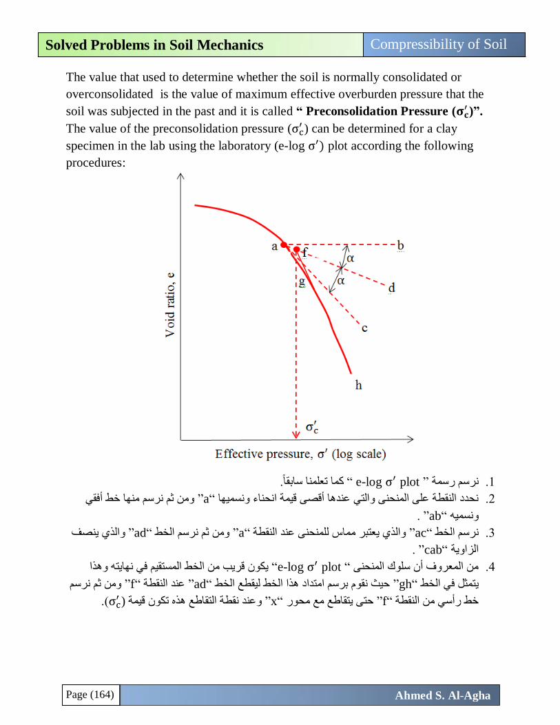
Page (164)
Compressibility of Soil Solved Problems in Soil Mechanics
Ahmed S. Al-Agha
The value that used to determine whether the soil is normally consolidated or
overconsolidated is the value of maximum effective overburden pressure that the
soil was subjected in the past and it is called “ Preconsolidation Pressure (𝛔𝐜′ )”.
The value of the preconsolidation pressure (σc′ ) can be determined for a clay
specimen in the lab using the laboratory (e-log σ′) plot according the following
procedures:
كما تعلمنا سابقاً. “ e-log σ′ plot ” نرسم رسمة .1
ومن ثم نرسم منها خط أفقي ”a“انحناء ونسميها نحدد النقطة على المنحنى والتي عندها أقصى قيمة .2
. ”ab“ونسميه
ينصف والذي ”ad“ومن ثم نرسم الخط ”a“والذي يعتبر مماس للمنحنى عند النقطة ”ac“نرسم الخط .3
. ”cab“الزاوية
يكون قريب من الخط المستقيم في نهايته وهذا e-log σ′ plot“ “من المعروف أن سلوك المنحنى .4
ومن ثم نرسم ”f“عند النقطة ”ad“حيث نقوم برسم امتداد هذا الخط ليقطع الخط ”gh“يتمثل في الخط
σcة التقاطع هذه تكون قيمة وعند نقط ”x“ حتى يتقاطع مع محور ”f“خط رأسي من النقطة ′ ).)
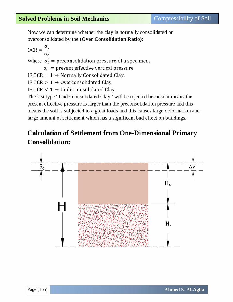
Page (165)
Compressibility of Soil Solved Problems in Soil Mechanics
Ahmed S. Al-Agha
Now we can determine whether the clay is normally consolidated or
overconsolidated by the (Over Consolidation Ratio):
OCR =σc
′
σo′
Where σc′ = preconsolidation pressure of a specimen.
σo′ = present effective vertical pressure.
IF OCR = 1 → Normally Consolidated Clay.
IF OCR > 1 → Overconsolidated Clay.
IF OCR < 1 → Underconsolidated Clay.
The last type “Underconsolidated Clay” will be rejected because it means the
present effective pressure is larger than the preconsolidation pressure and this
means the soil is subjected to a great loads and this causes large deformation and
large amount of settlement which has a significant bad effect on buildings.
Calculation of Settlement from One-Dimensional Primary
Consolidation:
Hv
Hs
Sc ∆V
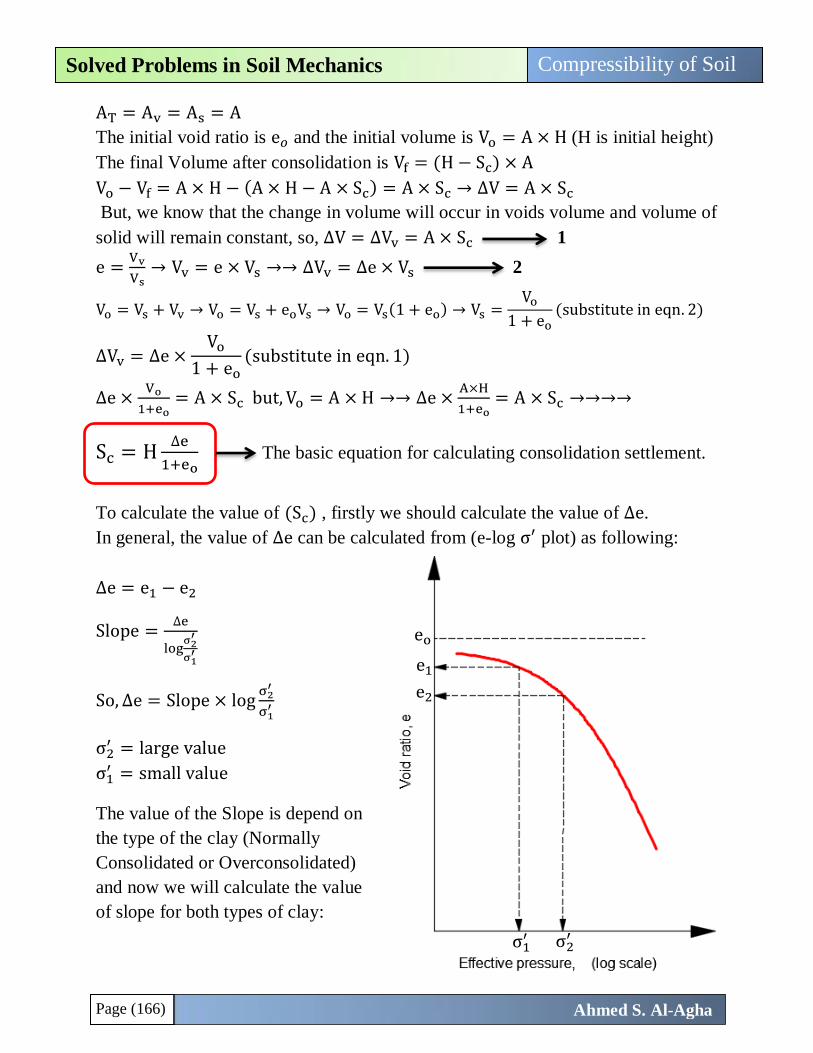
Page (166)
Compressibility of Soil Solved Problems in Soil Mechanics
Ahmed S. Al-Agha
AT = Av = As = A
The initial void ratio is e𝑜 and the initial volume is Vo = A × H (H is initial height)
The final Volume after consolidation is Vf = (H − Sc) × A
Vo − Vf = A × H − (A × H − A × Sc) = A × Sc → ∆V = A × Sc
But, we know that the change in volume will occur in voids volume and volume of
solid will remain constant, so, ∆V = ∆Vv = A × Sc 1
e =Vv
Vs→ Vv = e × Vs →→ ∆Vv = ∆e × Vs 2
Vo = Vs + Vv → Vo = Vs + eoVs → Vo = Vs(1 + eo) → Vs =Vo
1 + eo(substitute in eqn. 2)
∆Vv = ∆e ×Vo
1 + eo(substitute in eqn. 1)
∆e ×Vo
1+eo= A × Sc but, Vo = A × H →→ ∆e ×
A×H
1+eo= A × Sc →→→→
Sc = H∆e
1+eo The basic equation for calculating consolidation settlement.
To calculate the value of (Sc) , firstly we should calculate the value of ∆e.
In general, the value of ∆e can be calculated from (e-log σ′ plot) as following:
∆e = e1 − e2
Slope =∆e
logσ2
′
σ1′
So, ∆e = Slope × logσ2
′
σ1′
σ2′ = large value
σ1′ = small value
The value of the Slope is depend on
the type of the clay (Normally
Consolidated or Overconsolidated)
and now we will calculate the value
of slope for both types of clay:
eo
e1
e2
σ1′ σ2
′
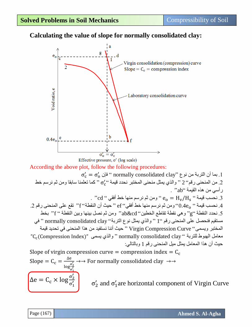
Page (167)
Compressibility of Soil Solved Problems in Soil Mechanics
Ahmed S. Al-Agha
Calculating the value of slope for normally consolidated clay:
According the above plot, follow the following procedures:
σc فإن ”normally consolidated clay “ نوعبما أن التربة من .1′ = σo
′
σc “ نحدد قيمة والذي يمثل منحنى المختبر ”2 “ من المنحنى رقم .2علمنا سابقا ومن ثم نرسم خط كما ت ”′
. ”ab “ رأسي من هذه القيمة
eo “ نحسب قيمة .3 = Hv/Hs “ ومن ثم نرسم منها خط أفقي “ cd” .
.2تقع على المنحنى رقم ”f “ حيث أن النقطة ”ef “ ومن ثم نرسم منها خط أفقي“ 0.4eo “ نحسب قيمة .4
بخط ”f “م نصل بينها وبين النقطة ثومن ”ab&cd “ وهي نقطة تقاطع الخطين ”g“ نحدد النقطة .5
في ”normally consolidated clay “ يمثل نوع التربة والذي ”1 “ مستقيم فنحصل على المنحنى رقم
تحديد قيمة حيث أننا نستفيد من هذا المنحنى في ”Virgin Compression Curve “ ىالمختبر ويسم
”Cc(Compression Index)” والذي يسمى ”normally consolidated clay “ معامل الهبوط للتربة
وبالتالي: 1حيث أن هذا المعامل يمثل ميل المنحنى رقم
Slope of virgin compression curve = compression index = Cc
Slope = Cc =∆e
logσ2
′
σ1′
→→ For normally consolidated clay →→
∆e = Cc × logσ2
′
σ1′
σ2′ and σ1
′ are horizontal component of Virgin Curve
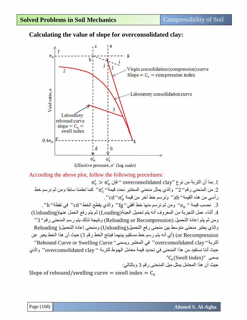
Page (168)
Compressibility of Soil Solved Problems in Soil Mechanics
Ahmed S. Al-Agha
Calculating the value of slope for overconsolidated clay:
According the above plot, follow the following procedures:
σc فإن ”overconsolidated clay “ بما أن التربة من نوع .1′ > σo
′
σc “نحدد قيمة المختبر والذي يمثل منحنى ”2 “من المنحنى رقم .2كما تعلمنا سابقا ومن ثم نرسم خط ”′
σoونرسم خط آخر من قيمة ”ab “رأسي من هذه القيمة ′ “ cd”.
.”h “في نقطة ”cd “والذي يقطع الخط ”fg “ومن ثم نرسم منها خط أفقي “ eo “نحسب قيمة .3
( Unloading( ثم يتم رفع الحمل عنها)Loadingينة)أثناء عمل التجربة من المعروف أنه يتم تحميل الع .4
”3 “( ونتيجة لذلك يتم رسم المنحنى رقم Reloading or Recompression) ومن ثم يتم إعادة التحميل
Reloading( ومنحنى إعادة التحميل)Unloadingالتحميل)والذي يعتبر منحنى متوسط بين منحنى رفع
or Recompression )( حيث أن هذا الخط يعبر عن 3سم خط مستقيم بينهما فينتج الخط رقم )أي أنه يتم ر
”Rebound Curve or Swelling Curve “في المختبر ويسمى ”overconsolidated clay “التربة
والذي ”overconsolidated clay “حيث أننا نستفيد من هذا المنحنى في تحديد قيمة معامل الهبوط للتربة
”Cs(Swell Index)”يسمى
وبالتالي: 3حيث أن هذا المعامل يمثل ميل المنحنى رقم
Slope of rebound/swelling curve = swell index = Cs
e
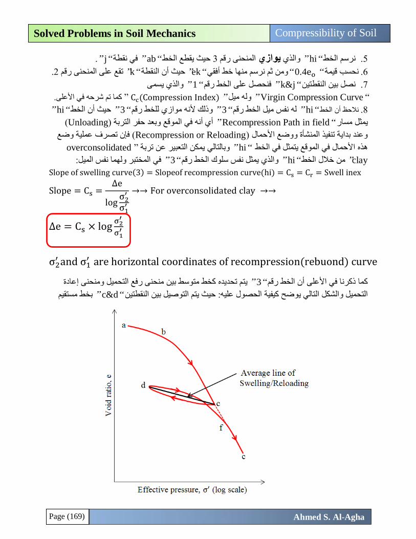
Page (169)
Compressibility of Soil Solved Problems in Soil Mechanics
Ahmed S. Al-Agha
.”j “في نقطة ”ab “ حيث يقطع الخط 3المنحنى رقم يوازيوالذي ”hi “نرسم الخط .5
.2تقع على المنحنى رقم ”k“النقطة حيث أن ”ek“ثم نرسم منها خط أفقي ومن“ 0.4eo “نحسب قيمة .6
والذي يسمى ”1 “فنحصل على الخط رقم ”k&j “نصل بين النقطتين .7
“ Virgin Compression Curve” ميل وله”” Cc(Compression Index) .كما تم شرحه في األعلى
”hi “ حيث أن الخط ”3 “ه موازي للخط رقم وذلك ألن ”3 “له نفس ميل الخط رقم ”hi “نالحظ أن الخط .8
(Unloadingد حفر التربة )وبعأي أنه في الموقع ”Recompression Path in field “يمثل مسار
( فإن تصرف عملية وضع Recompression or Reloadingوعند بداية تنفيذ المنشأة ووضع األحمال )
overconsolidated ” ن تربةوبالتالي يمكن التعبير ع ”hi “األحمال في الموقع يتمثل في الخط هذه
clay” من خالل الخط“ hi” في المختبر ولهما نفس الميل ”3 “والذي يمثل نفس سلوك الخط رقم:
Slope of swelling curve(3) = Slopeof recompression curve(hi) = Cs = Cr = Swell inex
Slope = Cs =∆e
logσ2
′
σ1′
→→ For overconsolidated clay →→
∆e = Cs × logσ2
′
σ1′
σ2′ and σ1
′ are horizontal coordinates of recompression(rebuond) curve
منحنى رفع التحميل ومنحنى إعادة كخط متوسط بين هيتم تحديد ”3 “أن الخط رقم كما ذكرنا في األعلى
بخط مستقيم ”c&d “الحصول عليه: حيث يتم التوصيل بين النقطتين التحميل والشكل التالي يوضح كيفية
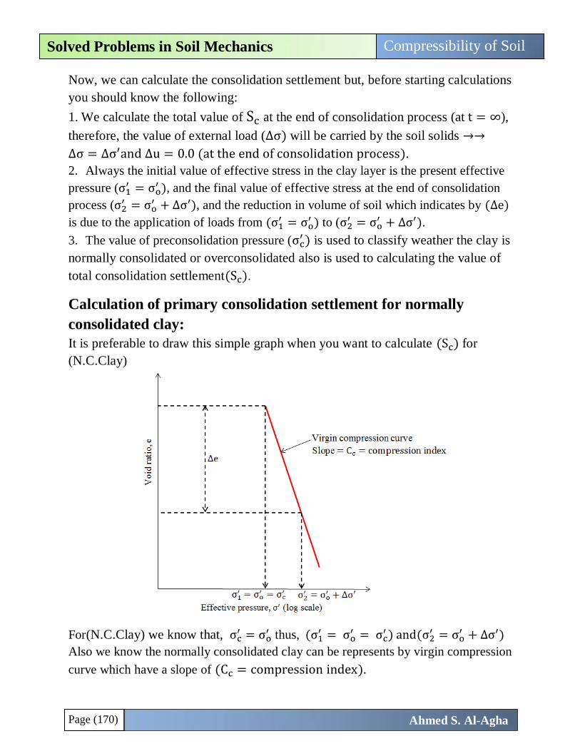
Page (170)
Compressibility of Soil Solved Problems in Soil Mechanics
Ahmed S. Al-Agha
Now, we can calculate the consolidation settlement but, before starting calculations
you should know the following:
1. We calculate the total value of Sc at the end of consolidation process (at t = ∞),
therefore, the value of external load (∆σ) will be carried by the soil solids →→
∆σ = ∆σ′and ∆u = 0.0 (at the end of consolidation process).
2. Always the initial value of effective stress in the clay layer is the present effective
pressure (σ1′ = σo
′ ), and the final value of effective stress at the end of consolidation
process (σ2′ = σo
′ + ∆σ′), and the reduction in volume of soil which indicates by (∆e)
is due to the application of loads from (σ1′ = σo
′ ) to (σ2′ = σo
′ + ∆σ′).
3. The value of preconsolidation pressure (σc′ ) is used to classify weather the clay is
normally consolidated or overconsolidated also is used to calculating the value of
total consolidation settlement(Sc).
Calculation of primary consolidation settlement for normally
consolidated clay:
It is preferable to draw this simple graph when you want to calculate (Sc) for
(N.C.Clay)
For(N.C.Clay) we know that, σc′ = σo
′ thus, (σ1′ = σo
′ = σc′ ) and(σ2
′ = σo′ + ∆σ′)
Also we know the normally consolidated clay can be represents by virgin compression
curve which have a slope of (Cc = compression index).
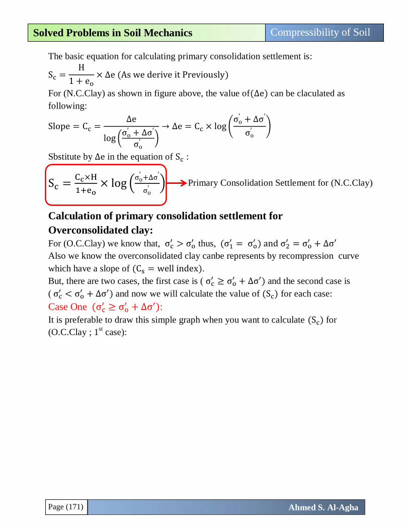
Page (171)
Compressibility of Soil Solved Problems in Soil Mechanics
Ahmed S. Al-Agha
The basic equation for calculating primary consolidation settlement is:
Sc =H
1 + eo× ∆e (As we derive it Previously)
For (N.C.Clay) as shown in figure above, the value of(∆e) can be claculated as
following:
Slope = Cc =∆e
log (σo
′ + ∆σ′
σo′ )
→ ∆e = Cc × log (σo
′ + ∆σ′
σo′
)
Sbstitute by ∆e in the equation of Sc :
Sc =Cc×H
1+eo× log (
σo′ +∆σ′
σo′
)
Calculation of primary consolidation settlement for
Overconsolidated clay:
For (O.C.Clay) we know that, σc′ > σo
′ thus, (σ1′ = σo
′ ) and σ2′ = σo
′ + ∆σ′
Also we know the overconsolidated clay canbe represents by recompression curve
which have a slope of (Cs = well index).
But, there are two cases, the first case is ( σc′ ≥ σo
′ + ∆σ′) and the second case is
( σc′ < σo
′ + ∆σ′) and now we will calculate the value of (Sc) for each case:
Case One (σc′ ≥ σo
′ + ∆σ′):
It is preferable to draw this simple graph when you want to calculate (Sc) for
(O.C.Clay ; 1st case):
Primary Consolidation Settlement for (N.C.Clay)

Page (172)
Compressibility of Soil Solved Problems in Soil Mechanics
Ahmed S. Al-Agha
σ1′ = σo
′ and σ2′ = σo
′ + ∆σ′
We note from the above graph, the consolidation settlement occur in the
overconsolidated curve (recompression curve) before reaching the normally
consolidated curve (virgin curve), this is case one.
The value of (∆e) can be claculated as following:
Slope = Cs =∆e
log (σo
′ + ∆σ′
σo′ )
→ ∆e = Cs × log (σo
′ + ∆σ′
σo′
)
Sbstitute by ∆e in the equation of Sc:
Sc =Cs×H
1+eo× log (
σo′ +∆σ′
σo′
)
We note that, the value of (∆e) is very small if we compare it with (∆e) for
(N.C.Clay).
Primary Consolidation Settlement for (O.C.Clay 1st case)
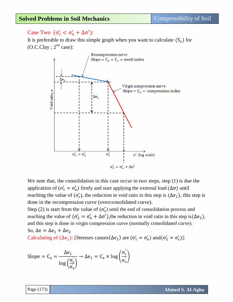
Page (173)
Compressibility of Soil Solved Problems in Soil Mechanics
Ahmed S. Al-Agha
Case Two (σc′ < σo
′ + ∆σ′):
It is preferable to draw this simple graph when you want to calculate (Sc) for
(O.C.Clay ; 2nd
case):
We note that, the consolidation in this case occur in two steps, step (1) is due the
application of (σ1′ = σo
′ ) firstly and start applying the external load (∆σ) until
reaching the value of (σc′ ), the reduction in void ratio in this step is (∆e1), this step is
done in the recompression curve (overconsolidated curve).
Step (2) is start from the value of (σc′ ) until the end of consolidation process and
reaching the value of (σ2′ = σo
′ + ∆σ′),the reduction in void ratio in this step is(∆e2),
and this step is done in virgin compression curve (normally consolidated curve).
So, ∆e = ∆e1 + ∆e2
Calculating of (∆e1): [Stresses causes(∆e1) are (σ1′ = σo
′ ) and(σ2′ = σc
′ )]:
Slope = Cs =∆e1
log (σc
′
σo′ )
→ ∆e1 = Cs × log (σc
′
σo′)
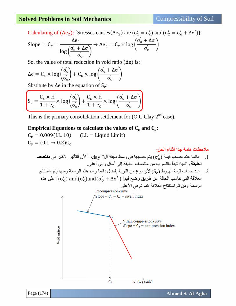
Page (174)
Compressibility of Soil Solved Problems in Soil Mechanics
Ahmed S. Al-Agha
Calculating of (∆e2): [Stresses causes(∆e2) are (σ1′ = σc
′ ) and(σ2′ = σo
′ + ∆σ′)]:
Slope = Cc =∆e2
log (σo
′ + ∆σ′
σc′ )
→ ∆e2 = Cc × log (σo
′ + ∆σ′
σc′
)
So, the value of total reduction in void ratio (∆e) is:
∆e = Cs × log (σc
′
σo′) + Cc × log (
σo′ + ∆σ′
σc′
)
Sbstitute by ∆e in the equation of Sc:
Sc =Cs × H
1 + eo× log (
σc′
σo′) +
Cc × H
1 + eo× log (
σo′ + ∆σ′
σc′
)
This is the primary consolidation settlement for (O.C.Clay 2nd
case).
Empirical Equations to calculate the values of 𝐂𝐜 and 𝐂𝐬:
Cc = 0.009(LL. 10) (LL = Liquid Limit)
Cs = (0.1 → 0.2)Cc
مالحظات هامة جدا أثناء الحل:
σoدائما عند حساب قيمة .1′ منتصف تأثير األكبر في ألن ال “ clay ”( يتم حسابها في وسط طبقة ال(
بدأ بالتسرب من منتصف الطبقة إلى أسفل وإلى أعلى.توالمياه الطبقة
استنتاج( ألي نوع من التربة يفضل دائما رسم هذه الرسمة ومنها يتم Scالهبوط )عند حساب قيمة .2
σo [العالقة التي تناسب الحالة عن طريق وضع قيم′ ) and(σc
′ )and(σo′ + ∆σ′ ))[ على هذه
الرسمة ومن ثم استنتاج العالقة كما تم في األعلى.
Page (175)
Compressibility of Soil Solved Problems in Soil Mechanics
Ahmed S. Al-Agha
σc)ل في األعلى أن قيمة كحيث نرى من الش′ تكون دائما بين المنحنيين ألنها الحد الفاصل بين نوعي التربة (
(N.C.Clay and O.C.Clay) ويتم حساب قيم] σo′ ) and(σo
′ + ∆σ′ ))[ ووضعها على المنحنى ومن
ثم استنتاج العالقة كما تم شرحه في األعلى.
إذا كان يوجد لدينا حمل غير متوزع على كامل مقطع التربة ) مثل قاعدة منفصلة أو لبشة خرسانية أو أي .3
لكن عند حساب قيم الهبوط فإن . (CH.10)انظر مقدمة حمل آخر( فإن ذلك الحمل يتناقص كلما زاد العمق
( في بداية الطبقة ′σ∆)( يجب أن تكون كمتوسط لكل طبقة الطين, لذلك في هذه الحالة سوف نجد′σ∆ة )قيم
ومن ثم إيجاد ( CH.10كما تم دراسته في القاعدة منتصف)أسفل وفي منتصف الطبقة وفي نهاية الطبقة
متوسط هذه القيم كما يلي:
Using Simpson’s rule, the value of ∆σav′ can be estimated as following:
∆σav′ =
∆σt′ + 4∆σm
′ + ∆σb′
6
∆σt′ = Increase in effective stress at the top of clay layer.
∆σm′ = Increase in effective stress at the middle of clay layer.
∆σb′ = Increase in effective stress at the bottom of clay layer.
وسوف يتضح ذلك عند حل األسئلة. أما في حالة كون األحمال موزعة على كامل التربة فإن قيمة الحمل
(CH.10تقريبا إلى التربة وال تتناقص مع زيادة العمق وبالتالي نأخذها كما هي. )انظر مقدمة ةتنتقل ثابت
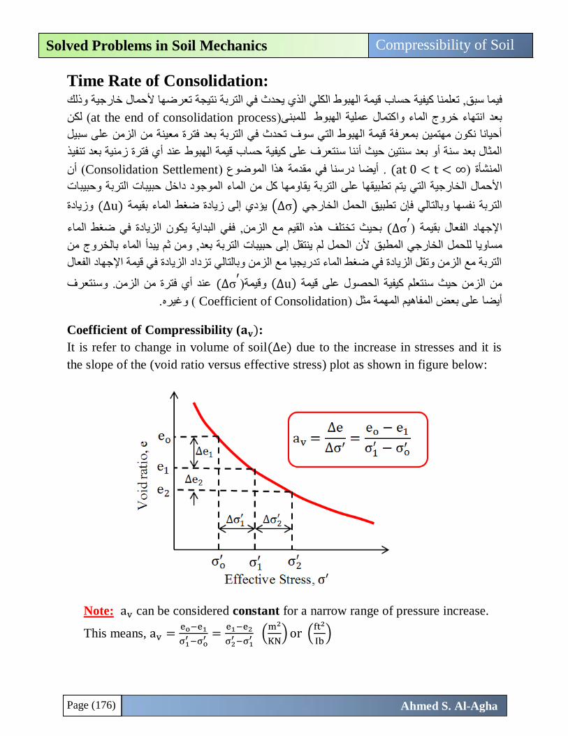
Page (176)
Compressibility of Soil Solved Problems in Soil Mechanics
Ahmed S. Al-Agha
Time Rate of Consolidation: وذلك تربة نتيجة تعرضها ألحمال خارجيةال قيمة الهبوط الكلي الذي يحدث في ما سبق, تعلمنا كيفية حسابفي
لكن ( at the end of consolidation processبعد انتهاء خروج الماء واكتمال عملية الهبوط للمبنى)
رة معينة من الزمن على سبيل أحيانا نكون مهتمين بمعرفة قيمة الهبوط التي سوف تحدث في التربة بعد فت
عند أي فترة زمنية بعد تنفيذ قيمة الهبوط حساب المثال بعد سنة أو بعد سنتين حيث أننا سنتعرف على كيفية
at 0)المنشأة ) < t < ( أن Consolidation Settlementأيضا درسنا في مقدمة هذا الموضوع ). ∞
اومها كل من الماء الموجود داخل حبيبات التربة وحبيبات األحمال الخارجية التي يتم تطبيقها على التربة يق
وزيادة (u∆)يؤدي إلى زيادة ضغط الماء بقيمة (σ∆)التربة نفسها وبالتالي فإن تطبيق الحمل الخارجي
σ∆)اإلجهاد الفعال بقيمة )′
في البداية يكون الزيادة في ضغط الماء ف ,مع الزمنهذه القيم حيث تختلف ب
ألن الحمل لم ينتقل إلى حبيبات التربة بعد, ومن ثم يبدأ الماء بالخروج من مل الخارجي المطبقمساويا للح
التربة مع الزمن وتقل الزيادة في ضغط الماء تدريجيا مع الزمن وبالتالي تزداد الزيادة في قيمة اإلجهاد الفعال
σ∆)وقيمة) (u∆)من الزمن حيث سنتعلم كيفية الحصول على قيمة ′
وسنتعرف ند أي فترة من الزمن.ع
وغيره. (Coefficient of Consolidation أيضا على بعض المفاهيم المهمة مثل )
Coefficient of Compressibility (𝐚𝐯):
It is refer to change in volume of soil(∆e) due to the increase in stresses and it is
the slope of the (void ratio versus effective stress) plot as shown in figure below:
Note: av can be considered constant for a narrow range of pressure increase.
This means, av =eo−e1
σ1′ −σo
′ =e1−e2
σ2′ −σ1
′ (m2
KN) or (
ft2
Ib)
Page (177)
Compressibility of Soil Solved Problems in Soil Mechanics
Ahmed S. Al-Agha
Coefficient of Volume Compressibility (𝐦𝐯):
It is the ratio of change in volume of a soil (∆e) to the unit initial volume due to
the increase in stresses (effective stresses) and is given by:
mv =eo − e1
1 + eo×
1
σ1′ − σo
′ =av
1 + eo
Now, when we want to calculate the value of (mv) we will use this formula:
mv =av
1 + eav
eav =eo+e1
2=
e1+e2
2
mv =
(eo − e1
σ1′ − σo
′ )
1 + (eo + e1
2)
=
(e1 − e2
σ2′ − σ1
′ )
1 + (e1 + e2
2)
(m2
KN) or (
ft2
Ib)
Coefficient of Consolidation (𝐜𝐯):
Is the parameter used to describe the rate at which saturated clay undergoes
consolidation, when subjected to an increase in pressure and can be calculated as
following:
cv =K
γw × mv (
m2
unit time) or (
ft2
unit time)
K = coefficient of permeability
There is another formula to calculate the value of (cv):
Tv =cv × t
Hdr2 → cv =
Tv × Hdr2
t
Tv = time factor (nondimensional number).
t = time required to reach a specific 𝐝𝐞𝐠𝐫𝐞𝐞 𝐨𝐟 𝐜𝐨𝐧𝐬𝐨𝐥𝐢𝐝𝐚𝐭𝐢𝐨𝐧.
Hdr = Drainage path of water through the clay layer (during consolidation)
Important Note:
The value of (cv) is always constant for the same soil, this means, the value of (cv)
is the same in lab and in field (for the same soil).
The value of (Hdr) can be determined according the following graph:
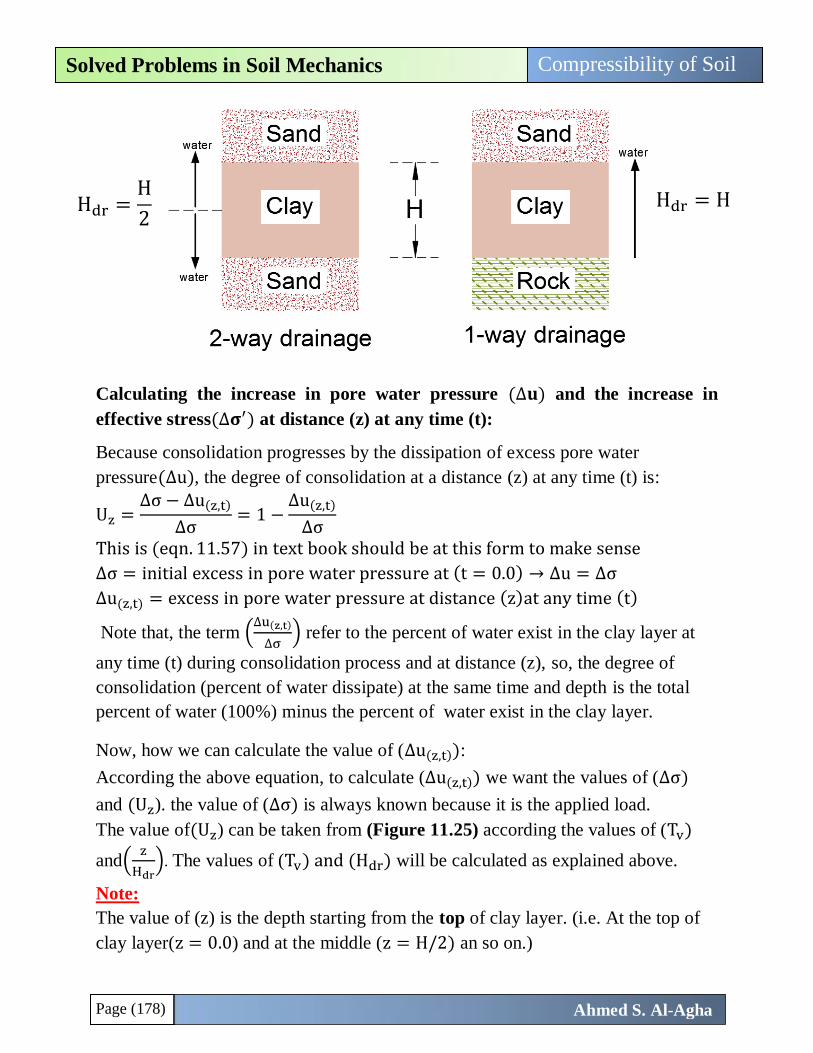
Page (178)
Compressibility of Soil Solved Problems in Soil Mechanics
Ahmed S. Al-Agha
Calculating the increase in pore water pressure (∆𝐮) and the increase in
effective stress(∆𝛔′) at distance (z) at any time (t):
Because consolidation progresses by the dissipation of excess pore water
pressure(∆u), the degree of consolidation at a distance (z) at any time (t) is:
Uz =∆σ − ∆u(z,t)
∆σ= 1 −
∆u(z,t)
∆σ
This is (eqn. 11.57) in text book should be at this form to make sense
∆σ = initial excess in pore water pressure at (t = 0.0) → ∆u = ∆σ
∆u(z,t) = excess in pore water pressure at distance (z)at any time (t)
Note that, the term (∆u(z,t)
∆σ) refer to the percent of water exist in the clay layer at
any time (t) during consolidation process and at distance (z), so, the degree of
consolidation (percent of water dissipate) at the same time and depth is the total
percent of water (100%) minus the percent of water exist in the clay layer.
Now, how we can calculate the value of (∆u(z,t)):
According the above equation, to calculate (∆u(z,t)) we want the values of (∆σ)
and (Uz). the value of (∆σ) is always known because it is the applied load.
The value of(Uz) can be taken from (Figure 11.25) according the values of (Tv)
and(z
Hdr). The values of (Tv) and (Hdr) will be calculated as explained above.
Note:
The value of (z) is the depth starting from the top of clay layer. (i.e. At the top of
clay layer(z = 0.0) and at the middle (z = H/2) an so on.)
Hdr =H
2 Hdr = H
Page (179)
Compressibility of Soil Solved Problems in Soil Mechanics
Ahmed S. Al-Agha
Now, we can get the value of(Uz) from (Figure 11.25) easily and we can calculate
the value of (∆u(z,t)) such that: (Uz = 1 −∆u(z,t)
∆σ) → ∆σ′(z,t) = ∆σ − ∆u(z,t).
Calculating the value of consolidation settlement at any time (t) during
consolidation process (𝐒𝐜(𝐭)):
Previously, we learn how to calculate the total amount of consolidation settlement
at the end of consolidation process (Sc(∞)) and now we want to calculate the value
of consolidation settlement before completion of consolidation process (Sc(t)), so,
the value of Sc(t) is percent of Sc(∞) such that: Sc(t)
Sc(∞)= percent , this percent called
[Average degree of consolidation (U)].
So, U =Sc(t)
Sc(∞)
Degree of consolidation (Uz) is the percent of water dissipates from the clay layer
at a certain depth (z) and at any time (t), But, the average degree of consolidation
(U) is the total amount of water dissipates from the whole clay layer at time (t).
The value of (U) is dependent on the value of (Tv), thus if one of them is known,
we can calculate the other value by one of the following three ways:
1. By equations (Not preferable):
For U = 0 to 60%, Tv =π
4(
U%
100)
2
For U > 60%, Tv = 1.781 − 0.933LOG(100 − U%)
2. By (Figure 11.26) (Not preferable)
3. By (Table 11.7) (Preferable and recommended).
Now, if we get the value of (U), we can calculate the value of (Sc(t)) as following:
(Sc(t)) = U × Sc(∞)
Important Notes:
t50 = time required to reach U = 50% , t60 = time required to reach U = 60% ….
All the following values are different in lab from the field for the same soil:
Hdr(lab) ≠ Hdr(field) , tlab ≠ t(field) , and Ulab ≠ U(field)
قات الكبيرة الموجودة في الواقع وأيضا بالطبألنه في المختبر تتم التجربة على عينة صغيرة من التربة مقارنة
.( في فترة زمنية قصيرة مقارنة بالواقع الذي قد تستمر فيه العملية لسنواتconsolidationتتم عملية ال)
But, the values of (cv, mv, and K) are the same in field and lab because they relates
to type of soil.
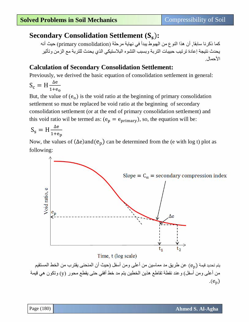
Page (180)
Compressibility of Soil Solved Problems in Soil Mechanics
Ahmed S. Al-Agha
Secondary Consolidation Settlement (𝐒𝐬): ( حيث أنه primary consolidationنهاية مرحلة )كما ذكرنا سابقا, أن هذا النوع من الهبوط يبدأ في
يحدث نتيجة إعادة ترتيب حبيبات التربة وبسبب التشوه البالستيكي الذي يحدث للتربة مع الزمن وتأثير
األحمال.
Calculation of Secondary Consolidation Settlement:
Previously, we derived the basic equation of consolidation settlement in general:
Sc = H∆e
1+eo
But, the value of (eo) is the void ratio at the beginning of primary consolidation
settlement so must be replaced be void ratio at the beginning of secondary
consolidation settlement (or at the end of primary consolidation settlement) and
this void ratio wil be termed as: (ep = eprimary), so, the equation will be:
Ss = H∆e
1+ep
Now, the values of (∆e)and(ep) can be determined from the (e with log t) plot as
following:
ومن أسفل )حيث أن المنحنى يقترب من الخط المستقيم عن طريق مد مماسين من أعلى (ep)يتم تحديد قيمة
وتكون هي قيمة ( yمن أعلى ومن أسفل( وعند نقطة تقاطع هذين الخطين يتم مد خط أفقي حتى يقطع محور )
(ep).
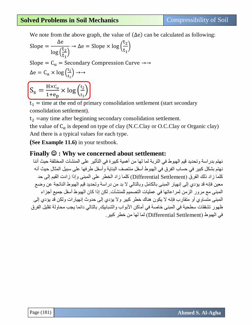
Page (181)
Compressibility of Soil Solved Problems in Soil Mechanics
Ahmed S. Al-Agha
We note from the above graph, the value of (∆e) can be calculated as following:
Slope =∆e
log (t2
t1)
→ ∆e = Slope × log (t2
t1)
Slope = Cα = Secondary Compression Curve →→
∆e = Cα × log (t2
t1) →→
Ss =H×Cα
1+ep× log (
t2
t1)
t1 = time at the end of primary consolidation settlement (start secondary
consolidation settlement).
t2 =any time after beginning secondary consolidation settlement.
the value of Cα is depend on type of clay (N.C.Clay or O.C.Clay or Organic clay)
And there is a typical values for each type.
(See Example 11.6) in your textbook.
Finally : Why we concerned about settlement:
نشآت المختلفة حيث أننا نهتم بدراسة وتحديد قيم الهبوط في التربة لما لها من أهمية كبيرة في التأثير على الم
طرفها على سبيل المثال حيث أنه وأسفلهبوط أسفل منتصف البناية نهتم بشكل كبير في حساب الفرق في ال
( كلما زاد الخطر على المبنى وإذا زادت القيم إلى حد Differential Settlement) كلما زاد ذلك الفرق
ة وتحديد قيم الهبوط الناتجة عن وضع سبالتالي ال بد من درامعين فإنه قد يؤدي إلى إنهيار المبنى بالكامل و
لمراعاتها في عمليات التصميم للمنشآت. لكن إذا كان الهبوط أسفل جميع أجزاء المبنى مع مرور الزمن
متقارب فإنه ال يكون هناك خطر كبير وال يؤدي إلى حدوث إنهيارات ولكن قد يؤدي إلى والمبنى متساوي أ
, بالتالي دائما يجب محاولة تقليل الفرق سطحية في المبنى خاصة في أماكن األبواب والشبابيكظهور تشققات
( لما لها من خطر كبير.Differential Settlement) في الهبوط

Page (182)
Compressibility of Soil Solved Problems in Soil Mechanics
Ahmed S. Al-Agha
51.
A clay layer in the field is 15 ft thick and is drained at the top only. Under a given
surcharge, the estimated consolidation settlement is 12.21 inch.
a) What is the average degree of consolidation for the clay layerwhen the
settlement is 3 inch?
b) If the average value of Cv for the pressure range is 0.003 cm2/sec, how long will
it take for 50% consolidation to occur?
c) If the 15 ft clay is drained from both sides, how long will it take for 50%
consolidation to occur?
Solution
Givens:
Hfield = 15 ft , drained at top only → Hdr = H = 15ft , Sc(t=∞) = 12ft
a) U = ???
U =Sc(t)
Sc(t=∞)=
3
12.21= 0.245 = 24.5% ✓.
b) If Cv = 0.003 cm2/ sec , and U = 50% → t =? ?
@ U = 50% → Tv = 0.197 (from 𝐓𝐚𝐛𝐥𝐞 𝟏𝟏. 𝟕)
Tv =Cv × t
Hdr2 →
الى سنتيميتر لتنسيق وتوحيد الوحدات Hdrبالسنتيمر المربع نقوم بتحويل وحدة Cvألن وحدة
Hdr = 15ft (1ft ≅ 30.48 cm) → Hdr = 15 × 30.48 = 457.2 cm.
→ t =0.197 × 457.22
0.003= 13726424.16 sec = 158.87 day = 0.435 year ✓.
c)
The required is the same as required (b), but here Hdr = 15
2= 7.5ft (both sides)
Hdr = 7.5ft (1ft ≅ 30.48 cm) → Hdr = 7.5 × 30.48 = 228.6 cm.
→ t =0.197 × 228.62
0.003= 3431606 sec = 39.7 day = 0.108 year ✓.
Page (183)
Compressibility of Soil Solved Problems in Soil Mechanics
Ahmed S. Al-Agha
52.
In a hydraulic oedometer 50% of the final settlement occurs in 25 miutes for a
sample 20 mm thick able to drain from one end (top only). Calculate the excess
pore water pressure measured by a pressure transducer at the impermeable
boundary 50 minutes after the application of a vertical stress increment of 75 kPa.
Solution
Givens:
U = 50% → Tv = 0.197 (from 𝐓𝐚𝐛𝐥𝐞 𝟏𝟏. 𝟕), t50 = 25 minutes
H = 20mm (draned from one side) → Hdr = H = 20mm
If ∆σ = 75 kPa (kN/m2), calculate ∆u(z=20mm ,t=50minutes)
At the impermeable boundary means at the bottom of the layer ( z = 20mm)
UZ =∆σ − ∆u(z,t)
∆σ
Now, to calculate ∆u(z,t) we need to calculate UZ from (Figure 11.25) according
the values of (z
Hdr) and Tv at the required time (50 minutes)
z
Hdr=
20
20= 1
Tv =Cv × t
Hdr2 → Tv,50minutes =
Cv × 50
202 (we need to calculate Cv)
From givens,
U = 50% → Tv = 0.197 and t50 = 25 minutes
Tv =Cv × t
Hdr2 → 0.197 =
Cv × 25
202 → Cv = 3.152 mm2/minutes
Now at t = 50 minutes, we can calculate Tv,50minutes →
Tv,50minutes =Cv × 50
202=
3.152 × 50
202= 0.394
Now accordinf the values of z
Hdr= 1 and Tv = 0.394, the value of UZ ≅ 0.52
(Figure 11.25)
UZ =∆σ − ∆u(z,t)
∆σ→ 0.52 =
75 − ∆u(z,t)
75→ ∆u(z,t) = 36 kN/m2 ✓.
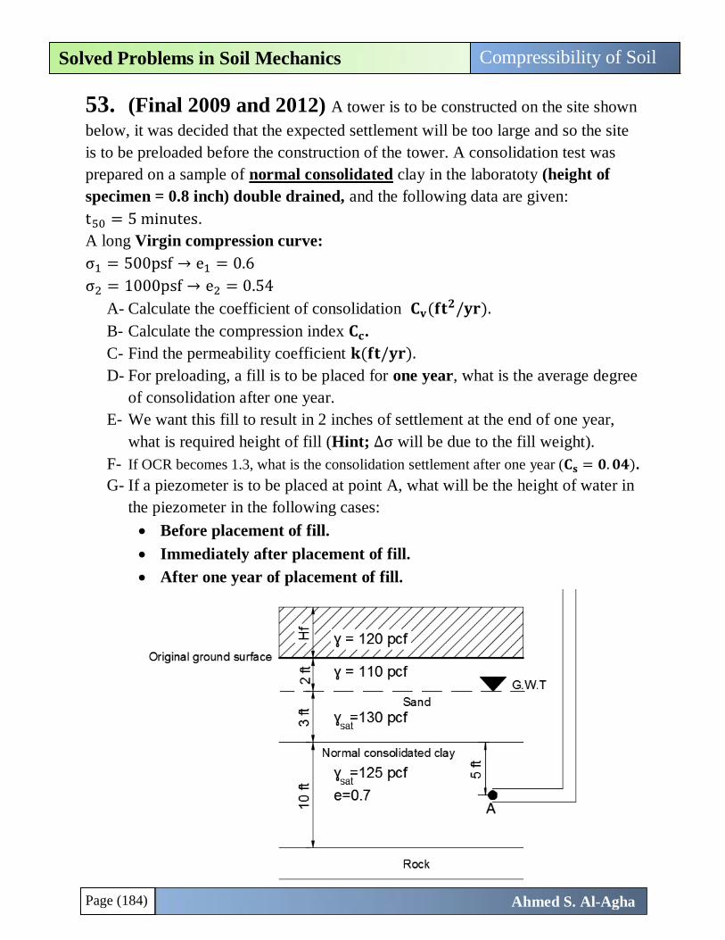
Page (184)
Compressibility of Soil Solved Problems in Soil Mechanics
Ahmed S. Al-Agha
53. (Final 2009 and 2012) A tower is to be constructed on the site shown
below, it was decided that the expected settlement will be too large and so the site
is to be preloaded before the construction of the tower. A consolidation test was
prepared on a sample of normal consolidated clay in the laboratoty (height of
specimen = 0.8 inch) double drained, and the following data are given:
t50 = 5 minutes.
A long Virgin compression curve:
σ1 = 500psf → e1 = 0.6
σ2 = 1000psf → e2 = 0.54
A- Calculate the coefficient of consolidation 𝐂𝐯(𝐟𝐭𝟐/𝐲𝐫).
B- Calculate the compression index 𝐂𝐜.
C- Find the permeability coefficient 𝐤(𝐟𝐭/𝐲𝐫).
D- For preloading, a fill is to be placed for one year, what is the average degree
of consolidation after one year.
E- We want this fill to result in 2 inches of settlement at the end of one year,
what is required height of fill (Hint; ∆σ will be due to the fill weight).
F- If OCR becomes 1.3, what is the consolidation settlement after one year (𝐂𝐬 = 𝟎. 𝟎𝟒).
G- If a piezometer is to be placed at point A, what will be the height of water in
the piezometer in the following cases:
Before placement of fill.
Immediately after placement of fill.
After one year of placement of fill.
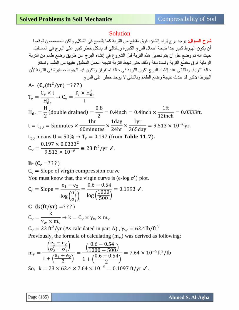
Page (185)
Compressibility of Soil Solved Problems in Soil Mechanics
Ahmed S. Al-Agha
Solution
يوجد برج ي راد إنشاؤه فوق مقطع من التربة كما يتضح في الشكل, ولكن المصممون توقعوا شرح السؤال:
أن يكون الهبوط كبير جدا نتيجة أحمال البرج الكبيرة وبالتالي قد يشكل خطر كبير على البرج في المستقبل
إنشاء البرج عن طريق وضع طمم من التربة حيث أنه تم وضع حل أن يتم تحميل هذه التربة قبل الشروع في
الرملية فوق مقطع التربة ولمدة سنة وذلك حتى تهبط التربة نتيجة الحمل المطبق عليها من الطمم وتستقر
حالة التربة, وبالتالي عند إنشاء البرج تكون التربة في حالة استقرار وتكون قيم الهبوط صغيرة في التربة ألن
دث نتيجة وضع الطمم وبالتالي ال يوجد خطر على البرج.الهبوط األكبر قد ح
A- (𝐂𝐯(𝐟𝐭𝟐/𝐲𝐫) =? ? ? )
Tv =Cv × t
Hdr2 → Cv =
Tv × Hdr2
t
Hdr =H
2(double drained) =
0.8
2= 0.4inch = 0.4inch ×
1ft
12inch= 0.0333ft.
t = t50 = 5minutes ×1hr
60minutes×
1day
24hr×
1yr
365day= 9.513 × 10⁻⁶yr.
t50 means U = 50% → Tv = 0.197 (from 𝐓𝐚𝐛𝐥𝐞 𝟏𝟏. 𝟕).
Cv =0.197 × 0.03332
9.513 × 10⁻⁶ ≅ 23 ft2/yr ✓.
B- (𝐂𝐜 =? ? ? )
Cc = Slope of virgin compression curve
You must know that, the virgin curve is (e-log σ′) plot.
Cc = Slope =e1 − e2
log (σ2
′
σ1′ )
=0.6 − 0.54
log (1000500
)= 0.1993 ✓.
C- (𝐤(𝐟𝐭/𝐲𝐫) =? ? ? )
Cv =k
γw × mv→ k = Cv × γw × mv
Cv = 23 ft2/yr (As calculated in part A) , γw = 62.4Ib/ft3
Previously, the formula of calculating (mv) was derived as following:
mv =
(e1 − e2
σ2′ − σ1
′ )
1 + (e1 + e2
2)
=(
0.6 − 0.541000 − 500
)
1 + (0.6 + 0.54
2)
= 7.64 × 10⁻⁵ft2/Ib
So, k = 23 × 62.4 × 7.64 × 10−5 = 0.1097 ft/yr ✓.
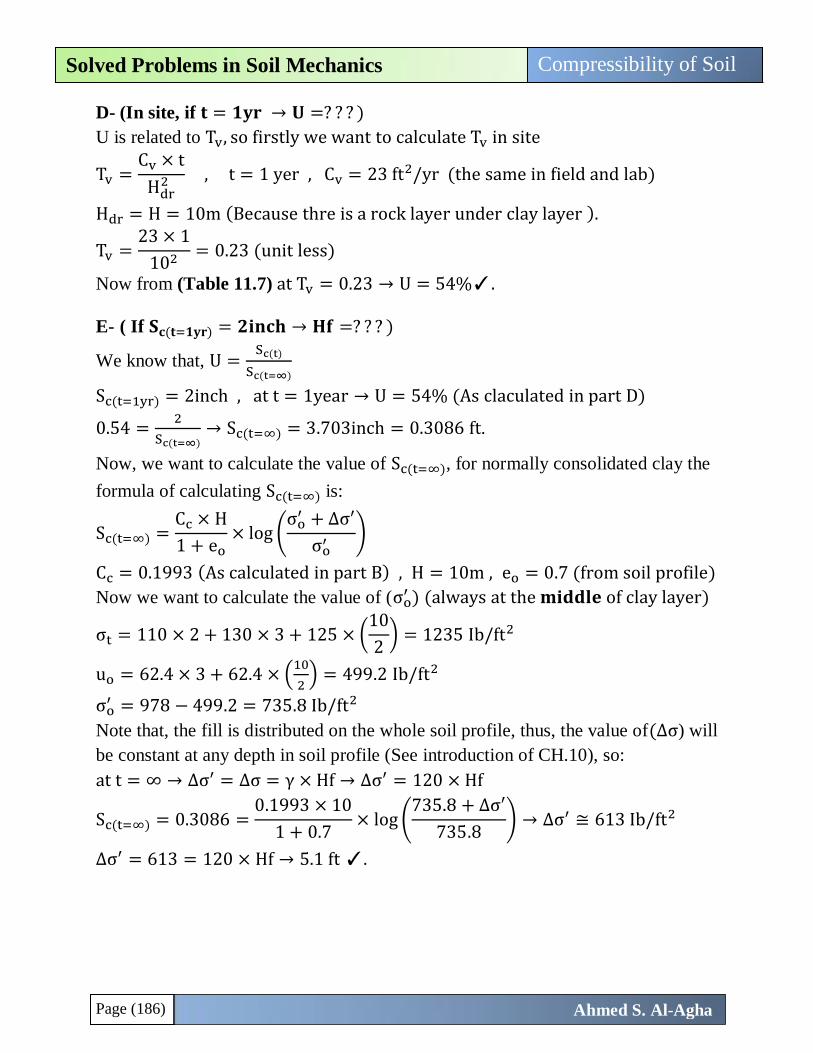
Page (186)
Compressibility of Soil Solved Problems in Soil Mechanics
Ahmed S. Al-Agha
D- (In site, if 𝐭 = 𝟏𝐲𝐫 → 𝐔 =? ? ? )
U is related to Tv, so firstly we want to calculate Tv in site
Tv =Cv × t
Hdr2 , t = 1 yer , Cv = 23 ft2/yr (the same in field and lab)
Hdr = H = 10m (Because thre is a rock layer under clay layer ).
Tv =23 × 1
102 = 0.23 (unit less)
Now from (Table 11.7) at Tv = 0.23 → U = 54%✓.
E- ( If 𝐒𝐜(𝐭=𝟏𝐲𝐫) = 𝟐𝐢𝐧𝐜𝐡 → 𝐇𝐟 =? ? ? )
We know that, U =Sc(t)
Sc(t=∞)
Sc(t=1yr) = 2inch , at t = 1year → U = 54% (As claculated in part D)
0.54 =2
Sc(t=∞)→ Sc(t=∞) = 3.703inch = 0.3086 ft.
Now, we want to calculate the value of Sc(t=∞), for normally consolidated clay the
formula of calculating Sc(t=∞) is:
Sc(t=∞) =Cc × H
1 + eo× log (
σo′ + ∆σ′
σo′ )
Cc = 0.1993 (As calculated in part B) , H = 10m , eo = 0.7 (from soil profile)
Now we want to calculate the value of (σo′ ) (always at the 𝐦𝐢𝐝𝐝𝐥𝐞 of clay layer)
σt = 110 × 2 + 130 × 3 + 125 × (10
2) = 1235 Ib/ft2
uo = 62.4 × 3 + 62.4 × (10
2) = 499.2 Ib/ft2
σo′ = 978 − 499.2 = 735.8 Ib/ft2
Note that, the fill is distributed on the whole soil profile, thus, the value of(∆σ) will
be constant at any depth in soil profile (See introduction of CH.10), so:
at t = ∞ → ∆σ′ = ∆σ = γ × Hf → ∆σ′ = 120 × Hf
Sc(t=∞) = 0.3086 =0.1993 × 10
1 + 0.7× log (
735.8 + ∆σ′
735.8) → ∆σ′ ≅ 613 Ib/ft2
∆σ′ = 613 = 120 × Hf → 5.1 ft ✓.
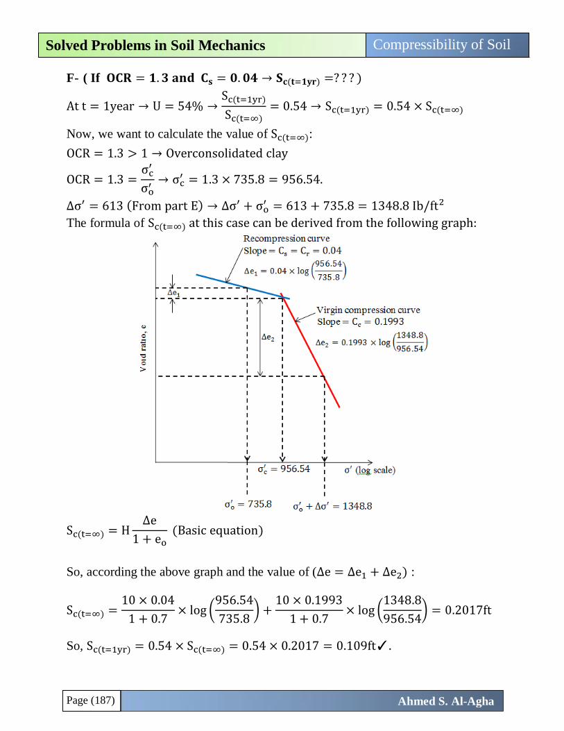
Page (187)
Compressibility of Soil Solved Problems in Soil Mechanics
Ahmed S. Al-Agha
F- ( If 𝐎𝐂𝐑 = 𝟏. 𝟑 𝐚𝐧𝐝 𝐂𝐬 = 𝟎. 𝟎𝟒 → 𝐒𝐜(𝐭=𝟏𝐲𝐫) =? ? ? )
At t = 1year → U = 54% →Sc(t=1yr)
Sc(t=∞)= 0.54 → Sc(t=1yr) = 0.54 × Sc(t=∞)
Now, we want to calculate the value of Sc(t=∞):
OCR = 1.3 > 1 → Overconsolidated clay
OCR = 1.3 =σc
′
σo′ → σc
′ = 1.3 × 735.8 = 956.54.
∆σ′ = 613 (From part E) → ∆σ′ + σo′ = 613 + 735.8 = 1348.8 Ib/ft2
The formula of Sc(t=∞) at this case can be derived from the following graph:
So, according the above graph and the value of (∆e = ∆e1 + ∆e2) :
Sc(t=∞) =10 × 0.04
1 + 0.7× log (
956.54
735.8) +
10 × 0.1993
1 + 0.7× log (
1348.8
956.54) = 0.2017ft
So, Sc(t=1yr) = 0.54 × Sc(t=∞) = 0.54 × 0.2017 = 0.109ft✓.
Sc(t=∞) = H∆e
1 + eo (Basic equation)
Page (188)
Compressibility of Soil Solved Problems in Soil Mechanics
Ahmed S. Al-Agha
G- (𝐡𝐩 =? ? ? 𝐢𝐧 𝐭𝐡𝐞 𝐟𝐨𝐥𝐥𝐨𝐰𝐢𝐧𝐠 𝐜𝐚𝐬𝐞𝐬)
In general, the piezometric height is the pressure head and (hp =u
γw)
And the general formula to calculate (u) is: (u = uo + ∆u)
The value of (uo) is the present pore water pressure due to the rise of G.W.T over
any point and is calculated in (part E) (uo = 499.2 Ib/ft2).
As we mentioned previously the value of (∆u) is varies with time and we will
calculate it at the different required three cases.
Case 1 (Before placement of fill)
Before placement of fill means (∆σ = 0.0 → ∆u = 0.0) →→→
u = 499.2 + 0.0 = 499.2 → hp =499.2
62.4= 8 ft✓.
Case 2 (Immediately after placement of fill)( 𝐭 = 𝟎. 𝟎):
In this case the whole value of (∆σ) will be carried by water because the load
doesn't transfer to the soil yet → (∆u = ∆σ = 613) →→
u = 499.2 + 613 = 1112.2 → hp =1112.2
62.4= 17.82 ft✓.
Case 3 (after one year of placement the fill)( 𝟎 < 𝐭 < ∞):
After completion of placement the loads the value of (∆σ) start to transfer to clay
and the water start to dissipate from the clay(∆u decreas with time) → (∆u < ∆σ)
To calculate the value of (∆u(z,t))at (t = 1yr)we will use the formula:
UZ =∆σ − ∆u(z,t)
∆σ
∆σ = initial value of ∆u = 613 Ib/ft2
∆u(z,t) =? ? ? at t = 1yr and zA = 5 ft (“z” start from the top of clay layer)
To calculate (∆u(5ft,1yr)) we must calculate the value of(UZ) →
The value of (UZ) can be calculated from (Figure 11.25) according the values of
(z
Hdr) and Tv. (Hdr = 10 , Tv(1yr) = 0.23) as calculated above
z
Hdr=
5
10= 0.5 , T v(1yr) = 0.23 → UZ ≅ 0.54 →→
0.54 =613 − ∆u(5ft,1yr)
613→ ∆u(5ft,1yr) = 281.98 Ib/ft2 →→→
u = 499.2 + 281.98 = 781.18 → hp =781.18
62.4= 12.52 ft✓.
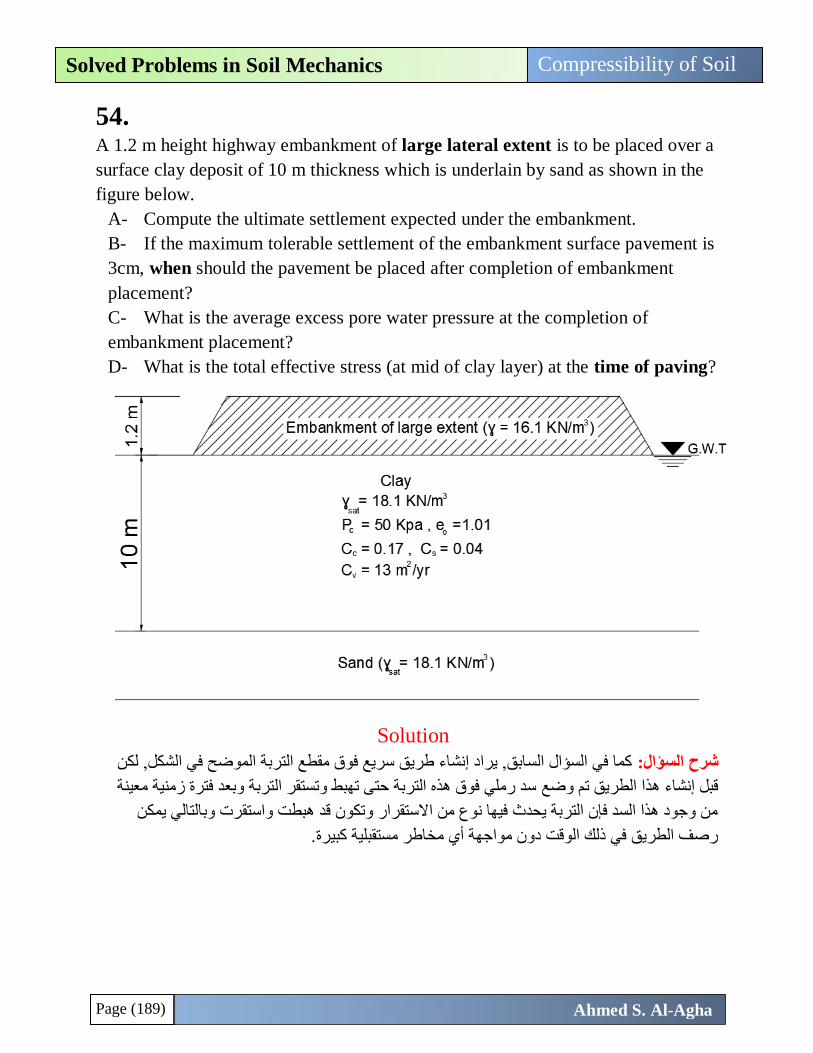
Page (189)
Compressibility of Soil Solved Problems in Soil Mechanics
Ahmed S. Al-Agha
54.
A 1.2 m height highway embankment of large lateral extent is to be placed over a
surface clay deposit of 10 m thickness which is underlain by sand as shown in the
figure below.
A- Compute the ultimate settlement expected under the embankment.
B- If the maximum tolerable settlement of the embankment surface pavement is
3cm, when should the pavement be placed after completion of embankment
placement?
C- What is the average excess pore water pressure at the completion of
embankment placement?
D- What is the total effective stress (at mid of clay layer) at the time of paving?
Solution
كما في السؤال السابق, يراد إنشاء طريق سريع فوق مقطع التربة الموضح في الشكل, لكن شرح السؤال:
سد رملي فوق هذه التربة حتى تهبط وتستقر التربة وبعد فترة زمنية معينة قبل إنشاء هذا الطريق تم وضع
من وجود هذا السد فإن التربة يحدث فيها نوع من االستقرار وتكون قد هبطت واستقرت وبالتالي يمكن
رصف الطريق في ذلك الوقت دون مواجهة أي مخاطر مستقبلية كبيرة.
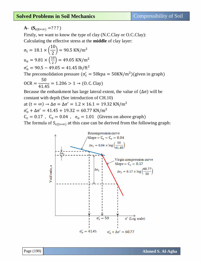
Page (190)
Compressibility of Soil Solved Problems in Soil Mechanics
Ahmed S. Al-Agha
A- (𝐒𝐜(𝐭=∞) =? ? ? )
Firstly, we want to know the type of clay (N.C.Clay or O.C.Clay):
Calculating the effective stress at the middle of clay layer:
σt = 18.1 × (10
2) = 90.5 KN/m2
uo = 9.81 × (10
2) = 49.05 KN/m2
σo′ = 90.5 − 49.05 = 41.45 Ib/ft2
The preconsolidation pressure (σc′ = 50kpa = 50KN/m2)(given in graph)
OCR =50
41.45= 1.206 > 1 → (O. C. Clay)
Because the embankment has large lateral extent, the value of (∆σ) will be
constant with depth (See introduction of CH.10)
at (t = ∞) → ∆σ = ∆σ′ = 1.2 × 16.1 = 19.32 KN/m2
σo′ + ∆σ′ = 41.45 + 19.32 = 60.77 KN/m2
Cc = 0.17 , Cs = 0.04 , eo = 1.01 (Givens on above graph)
The formula of Sc(t=∞) at this case can be derived from the following graph:
Page (191)
Compressibility of Soil Solved Problems in Soil Mechanics
Ahmed S. Al-Agha
So, according the above graph and the value of (∆e = ∆e1 + ∆e2):
Sc(t=∞) =10 × 0.04
1 + 1.01× log (
50
41.45) +
10 × 0.17
1 + 1.01× log (
60.77
50) →→
Sc(t=∞) = 0.0878m = 8.78cm✓.
B- (𝐭 =? ? ? 𝐢𝐟 𝐒𝐜(𝐭) = 𝟑𝐜𝐦):
We know that, U =Sc(t)
Sc(t=∞)=
3
8.78× 100 = 34.17%
(From Table 11.7 → at U = 34.16% → Tv ≅ 0.091)
Tv =Cv × t
Hdr2 (Cv = 13m2/yr , Hdr = H = 10m) Hdr = H →→
(Beacuse there is sand below the clay and fill pavement(prevent drainage) above)
0.091 =13 × t
102→ t = 0.7 yr = 255.5 day✓.
C- (∆𝐮(𝟓,𝟎.𝟎) =? ? ? )
Average excess (means at the mid of clay layer “at z = 5m”)
At the completion of embankment placement means (t = 0.0)
So, ∆u(5,0.0) = ∆σ = 19.32 KN/m2✓.
D- (𝛔𝐭′ =? ? ? 𝐚𝐭 𝐭(𝐭𝐢𝐦𝐞 𝐨𝐟 𝐩𝐚𝐯𝐞𝐦𝐞𝐧𝐭 “𝐩𝐚𝐫𝐭 𝐁 “) = 𝟎. 𝟕 𝐲𝐫):
σt′ = σo
′ + ∆σ′(z,t) (z = 5m , t = 0.7 yr)
To calculate (∆σ′(5m,0.7yr)), we must calculate(∆u(5m,0.7yr) )
UZ =∆σ − ∆u(5m,0.7yr)
∆σ , ∆σ = 19.32 KN/m2
z
Hdr=
5
10= 0.5 , T v(0.7yr) = 0.091 → UZ ≅ 0.23 (from 𝐅𝐢𝐠𝐮𝐫𝐞 𝟏𝟏. 𝟐𝟓) →→
0.23 =19.32 − ∆u(5m,0.7yr)
19.32→ ∆u(5m,0.7yr) = 14.87KN/m2 →
∆σ′(5m,0.7yr) = ∆σ − ∆u(5m,0.7yr) = 19.32 − 14.87 = 4.45KN/m2
σt′ = 41.45 + 4.45 = 45.9 KN/m2✓.
Sc(t=∞) = H∆e
1 + eo (Basic equation)
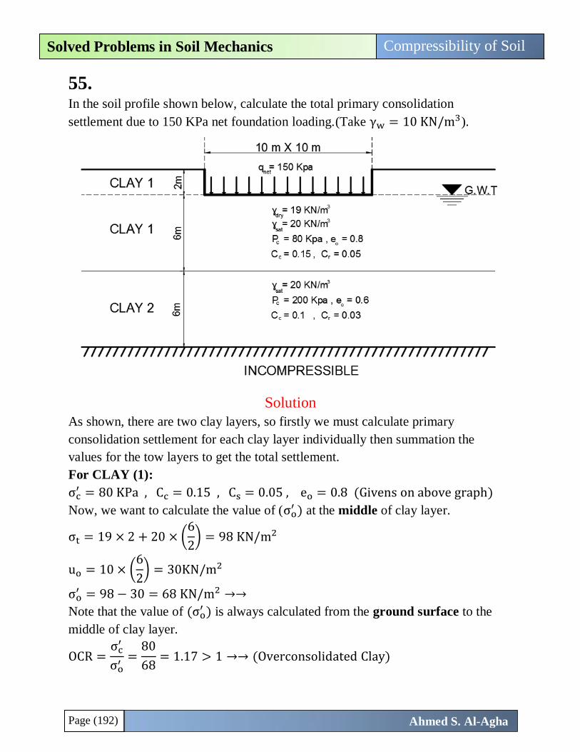
Page (192)
Compressibility of Soil Solved Problems in Soil Mechanics
Ahmed S. Al-Agha
55.
In the soil profile shown below, calculate the total primary consolidation
settlement due to 150 KPa net foundation loading.(Take γw = 10 KN/m3).
Solution
As shown, there are two clay layers, so firstly we must calculate primary
consolidation settlement for each clay layer individually then summation the
values for the tow layers to get the total settlement.
For CLAY (1):
σc′ = 80 KPa , Cc = 0.15 , Cs = 0.05 , eo = 0.8 (Givens on above graph)
Now, we want to calculate the value of (σo′ ) at the middle of clay layer.
σt = 19 × 2 + 20 × (6
2) = 98 KN/m2
uo = 10 × (6
2) = 30KN/m2
σo′ = 98 − 30 = 68 KN/m2 →→
Note that the value of (σo′ ) is always calculated from the ground surface to the
middle of clay layer.
OCR =σc
′
σo′
=80
68= 1.17 > 1 →→ (Overconsolidated Clay)
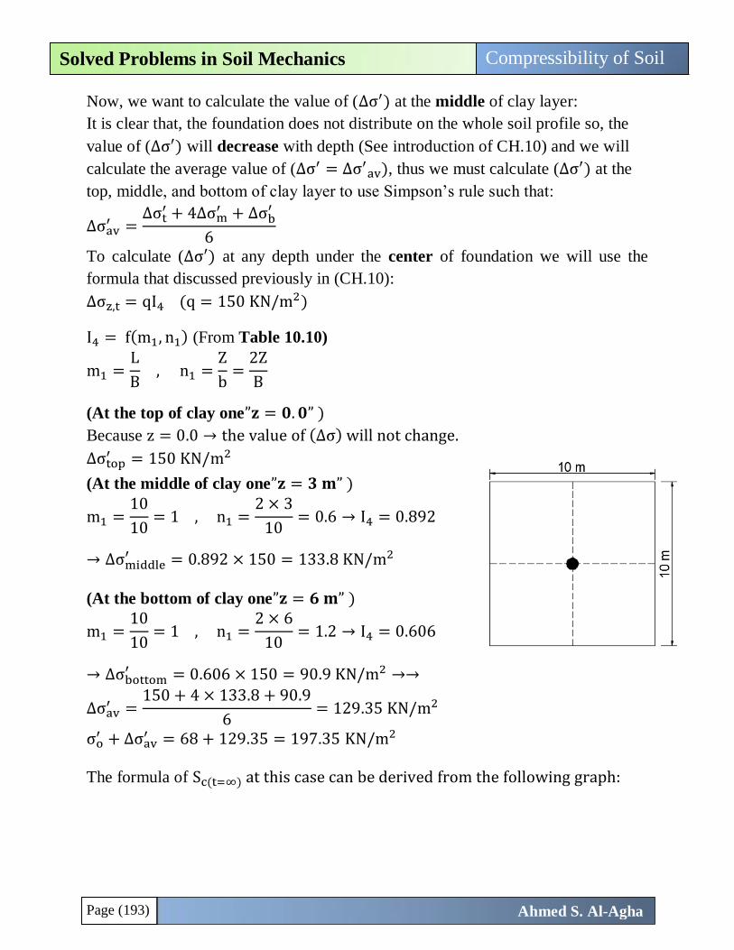
Page (193)
Compressibility of Soil Solved Problems in Soil Mechanics
Ahmed S. Al-Agha
Now, we want to calculate the value of (∆σ′) at the middle of clay layer:
It is clear that, the foundation does not distribute on the whole soil profile so, the
value of (∆σ′) will decrease with depth (See introduction of CH.10) and we will
calculate the average value of (∆σ′ = ∆σ′av), thus we must calculate (∆σ′) at the
top, middle, and bottom of clay layer to use Simpson’s rule such that:
∆σav′ =
∆σt′ + 4∆σm
′ + ∆σb′
6
To calculate (∆σ′) at any depth under the center of foundation we will use the
formula that discussed previously in (CH.10):
∆σz,t = qI4 (q = 150 KN/m2)
I4 = f(m1, n1) (From Table 10.10)
m1 =L
B , n1 =
Z
b=
2Z
B
(At the top of clay one”𝐳 = 𝟎. 𝟎” )
Because z = 0.0 → the value of (∆σ) will not change.
∆σtop′ = 150 KN/m2
(At the middle of clay one”𝐳 = 𝟑 𝐦” )
m1 =10
10= 1 , n1 =
2 × 3
10= 0.6 → I4 = 0.892
→ ∆σmiddle′ = 0.892 × 150 = 133.8 KN/m2
(At the bottom of clay one”𝐳 = 𝟔 𝐦” )
m1 =10
10= 1 , n1 =
2 × 6
10= 1.2 → I4 = 0.606
→ ∆σbottom′ = 0.606 × 150 = 90.9 KN/m2 →→
∆σav′ =
150 + 4 × 133.8 + 90.9
6= 129.35 KN/m2
σo′ + ∆σav
′ = 68 + 129.35 = 197.35 KN/m2
The formula of Sc(t=∞) at this case can be derived from the following graph:
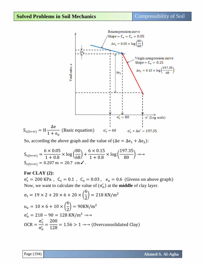
Page (194)
Compressibility of Soil Solved Problems in Soil Mechanics
Ahmed S. Al-Agha
So, according the above graph and the value of (∆e = ∆e1 + ∆e2):
Sc(t=∞) =6 × 0.05
1 + 0.8× log (
80
68) +
6 × 0.15
1 + 0.8× log (
197.35
80) →→
Sc(t=∞) = 0.207 m = 20.7 cm✓.
For CLAY (2):
σc′ = 200 KPa , Cc = 0.1 , Cs = 0.03 , eo = 0.6 (Givens on above graph)
Now, we want to calculate the value of (σo′ ) at the middle of clay layer.
σt = 19 × 2 + 20 × 6 + 20 × (6
2) = 218 KN/m2
uo = 10 × 6 + 10 × (6
2) = 90KN/m2
σo′ = 218 − 90 = 128 KN/m2 →→
OCR =σc
′
σo′ =
200
128= 1.56 > 1 →→ (Overconsolidated Clay)
Sc(t=∞) = H∆e
1 + eo (Basic equation)
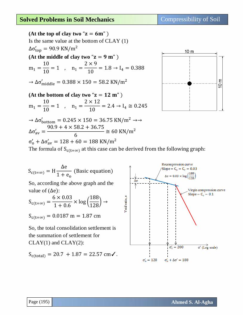
Page (195)
Compressibility of Soil Solved Problems in Soil Mechanics
Ahmed S. Al-Agha
(At the top of clay two “𝐳 = 𝟔𝐦” )
Is the same value at the bottom of CLAY (1)
∆σtop′ = 90.9 KN/m2
(At the middle of clay two “𝐳 = 𝟗 𝐦” )
m1 =10
10= 1 , n1 =
2 × 9
10= 1.8 → I4 = 0.388
→ ∆σmiddle′ = 0.388 × 150 = 58.2 KN/m2
(At the bottom of clay two “𝐳 = 𝟏𝟐 𝐦” )
m1 =10
10= 1 , n1 =
2 × 12
10= 2.4 → I4 ≅ 0.245
→ ∆σbottom′ = 0.245 × 150 = 36.75 KN/m2 →→
∆σav′ =
90.9 + 4 × 58.2 + 36.75
6≅ 60 KN/m2
σo′ + ∆σav
′ = 128 + 60 = 188 KN/m2
The formula of Sc(t=∞) at this case can be derived from the following graph:
So, according the above graph and the
value of (∆e):
Sc(t=∞) =6 × 0.03
1 + 0.6× log (
188
128) →
Sc(t=∞) = 0.0187 m = 1.87 cm
So, the total consolidation settlement is
the summation of settlement for
CLAY(1) and CLAY(2):
Sc(total) = 20.7 + 1.87 = 22.57 cm✓.
Sc(t=∞) = H∆e
1 + eo (Basic equation)
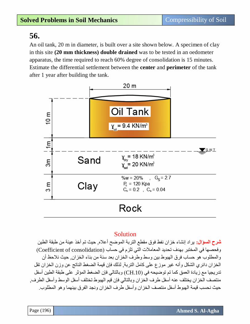
Page (196)
Compressibility of Soil Solved Problems in Soil Mechanics
Ahmed S. Al-Agha
56.
An oil tank, 20 m in diameter, is built over a site shown below. A specimen of clay
in this site (20 mm thickness) double drained was to be tested in an oedometer
apparatus, the time required to reach 60% degree of consolidation is 15 minutes.
Estimate the differential settlement between the center and perimeter of the tank
after 1 year after building the tank.
Solution
يراد إنشاء خزان نفط فوق مقطع التربة الموضح أعاله, حيث تم أخذ عينة من طبقة الطين شرح السؤال:
( Coefficient of consolidationوفحصها في المختبر بهدف تحديد المعامالت التي تلزم في حساب )
والمطلوب هو حساب فرق الهبوط بين وسط وطرف الخزان بعد سنة من بناء الخزان, حيث نالحظ أن
الخزان دائري الشكل وأنه غير موزع على كامل التربة, لذلك فإن قيمة الضغط الناتج عن وزن الخزان تقل
ضغط المؤثر على طبقة الطين أسفل ( وبالتالي فإن الCH.10تدريجيا مع زيادة العمق كما تم توضيحه في )
منتصف الخزان يختلف عنه أسفل طرف الخزان وبالتالي فإن قيم الهبوط تختلف أسفل الوسط وأسفل الطرف,
حيث نحسب قيمة الهبوط أسفل منتصف الخزان وأسفل طرف الخزان ونجد الفرق بينهما وهو المطلوب.
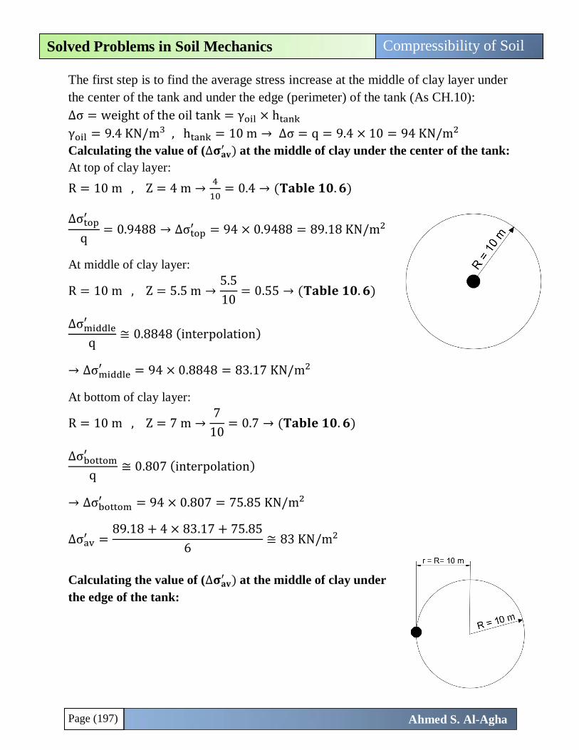
Page (197)
Compressibility of Soil Solved Problems in Soil Mechanics
Ahmed S. Al-Agha
The first step is to find the average stress increase at the middle of clay layer under
the center of the tank and under the edge (perimeter) of the tank (As CH.10):
∆σ = weight of the oil tank = γoil × htank
γoil = 9.4 KN/m3 , htank = 10 m → ∆σ = q = 9.4 × 10 = 94 KN/m2
Calculating the value of (∆𝛔𝐚𝐯′ ) at the middle of clay under the center of the tank:
At top of clay layer:
R = 10 m , Z = 4 m →4
10= 0.4 → (𝐓𝐚𝐛𝐥𝐞 𝟏𝟎. 𝟔)
∆σtop′
q= 0.9488 → ∆σtop
′ = 94 × 0.9488 = 89.18 KN/m2
At middle of clay layer:
R = 10 m , Z = 5.5 m →5.5
10= 0.55 → (𝐓𝐚𝐛𝐥𝐞 𝟏𝟎. 𝟔)
∆σmiddle′
q≅ 0.8848 (interpolation)
→ ∆σmiddle′ = 94 × 0.8848 = 83.17 KN/m2
At bottom of clay layer:
R = 10 m , Z = 7 m →7
10= 0.7 → (𝐓𝐚𝐛𝐥𝐞 𝟏𝟎. 𝟔)
∆σbottom′
q≅ 0.807 (interpolation)
→ ∆σbottom′ = 94 × 0.807 = 75.85 KN/m2
∆σav′ =
89.18 + 4 × 83.17 + 75.85
6≅ 83 KN/m2
Calculating the value of (∆𝛔𝐚𝐯′ ) at the middle of clay under
the edge of the tank:
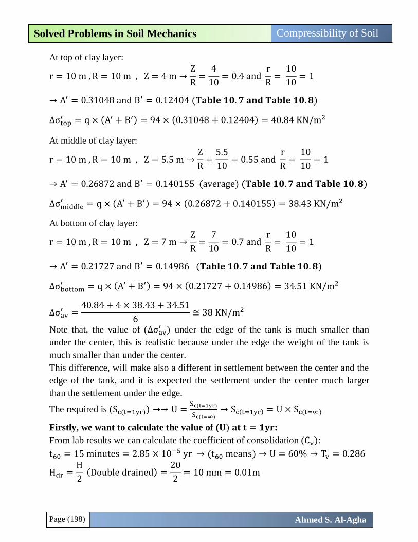
Page (198)
Compressibility of Soil Solved Problems in Soil Mechanics
Ahmed S. Al-Agha
At top of clay layer:
r = 10 m , R = 10 m , Z = 4 m →Z
R=
4
10= 0.4 and
r
R=
10
10= 1
→ A′ = 0.31048 and B′ = 0.12404 (𝐓𝐚𝐛𝐥𝐞 𝟏𝟎. 𝟕 𝐚𝐧𝐝 𝐓𝐚𝐛𝐥𝐞 𝟏𝟎. 𝟖)
∆σtop′ = q × (A′ + B′) = 94 × (0.31048 + 0.12404) = 40.84 KN/m2
At middle of clay layer:
r = 10 m , R = 10 m , Z = 5.5 m →Z
R=
5.5
10= 0.55 and
r
R=
10
10= 1
→ A′ = 0.26872 and B′ = 0.140155 (average) (𝐓𝐚𝐛𝐥𝐞 𝟏𝟎. 𝟕 𝐚𝐧𝐝 𝐓𝐚𝐛𝐥𝐞 𝟏𝟎. 𝟖)
∆σmiddle′ = q × (A′ + B′) = 94 × (0.26872 + 0.140155) = 38.43 KN/m2
At bottom of clay layer:
r = 10 m , R = 10 m , Z = 7 m →Z
R=
7
10= 0.7 and
r
R=
10
10= 1
→ A′ = 0.21727 and B′ = 0.14986 (𝐓𝐚𝐛𝐥𝐞 𝟏𝟎. 𝟕 𝐚𝐧𝐝 𝐓𝐚𝐛𝐥𝐞 𝟏𝟎. 𝟖)
∆σbottom′ = q × (A′ + B′) = 94 × (0.21727 + 0.14986) = 34.51 KN/m2
∆σav′ =
40.84 + 4 × 38.43 + 34.51
6≅ 38 KN/m2
Note that, the value of (∆σav′ ) under the edge of the tank is much smaller than
under the center, this is realistic because under the edge the weight of the tank is
much smaller than under the center.
This difference, will make also a different in settlement between the center and the
edge of the tank, and it is expected the settlement under the center much larger
than the settlement under the edge.
The required is (Sc(t=1yr)) →→ U =Sc(t=1yr)
Sc(t=∞)→ Sc(t=1yr) = U × Sc(t=∞)
Firstly, we want to calculate the value of (𝐔) 𝐚𝐭 𝐭 = 𝟏𝐲𝐫:
From lab results we can calculate the coefficient of consolidation (Cv):
t60 = 15 minutes = 2.85 × 10⁻⁵ yr → (t60 means) → U = 60% → Tv = 0.286
Hdr =H
2 (Double drained) =
20
2= 10 mm = 0.01m
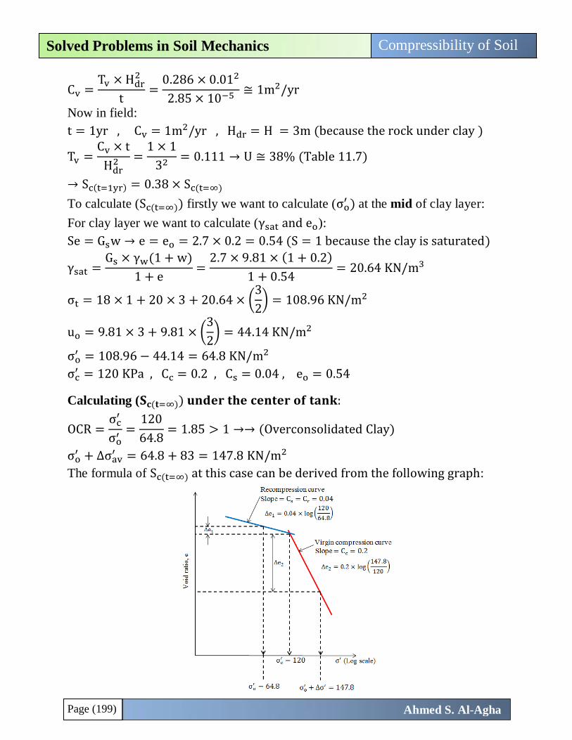
Page (199)
Compressibility of Soil Solved Problems in Soil Mechanics
Ahmed S. Al-Agha
Cv =Tv × Hdr
2
t=
0.286 × 0.012
2.85 × 10⁻⁵ ≅ 1m2/yr
Now in field:
t = 1yr , Cv = 1m2/yr , Hdr = H = 3m (because the rock under clay )
Tv =Cv × t
Hdr2 =
1 × 1
32 = 0.111 → U ≅ 38% (Table 11.7)
→ Sc(t=1yr) = 0.38 × Sc(t=∞)
To calculate (Sc(t=∞)) firstly we want to calculate (σo′ ) at the mid of clay layer:
For clay layer we want to calculate (γsat and eo):
Se = Gsw → e = eo = 2.7 × 0.2 = 0.54 (S = 1 because the clay is saturated)
γsat =Gs × γw(1 + w)
1 + e=
2.7 × 9.81 × (1 + 0.2)
1 + 0.54= 20.64 KN/m3
σt = 18 × 1 + 20 × 3 + 20.64 × (3
2) = 108.96 KN/m2
uo = 9.81 × 3 + 9.81 × (3
2) = 44.14 KN/m2
σo′ = 108.96 − 44.14 = 64.8 KN/m2
σc′ = 120 KPa , Cc = 0.2 , Cs = 0.04 , eo = 0.54
Calculating (𝐒𝐜(𝐭=∞)) 𝐮𝐧𝐝𝐞𝐫 𝐭𝐡𝐞 𝐜𝐞𝐧𝐭𝐞𝐫 𝐨𝐟 𝐭𝐚𝐧𝐤:
OCR =σc
′
σo′ =
120
64.8= 1.85 > 1 →→ (Overconsolidated Clay)
σo′ + ∆σav
′ = 64.8 + 83 = 147.8 KN/m2
The formula of Sc(t=∞) at this case can be derived from the following graph:
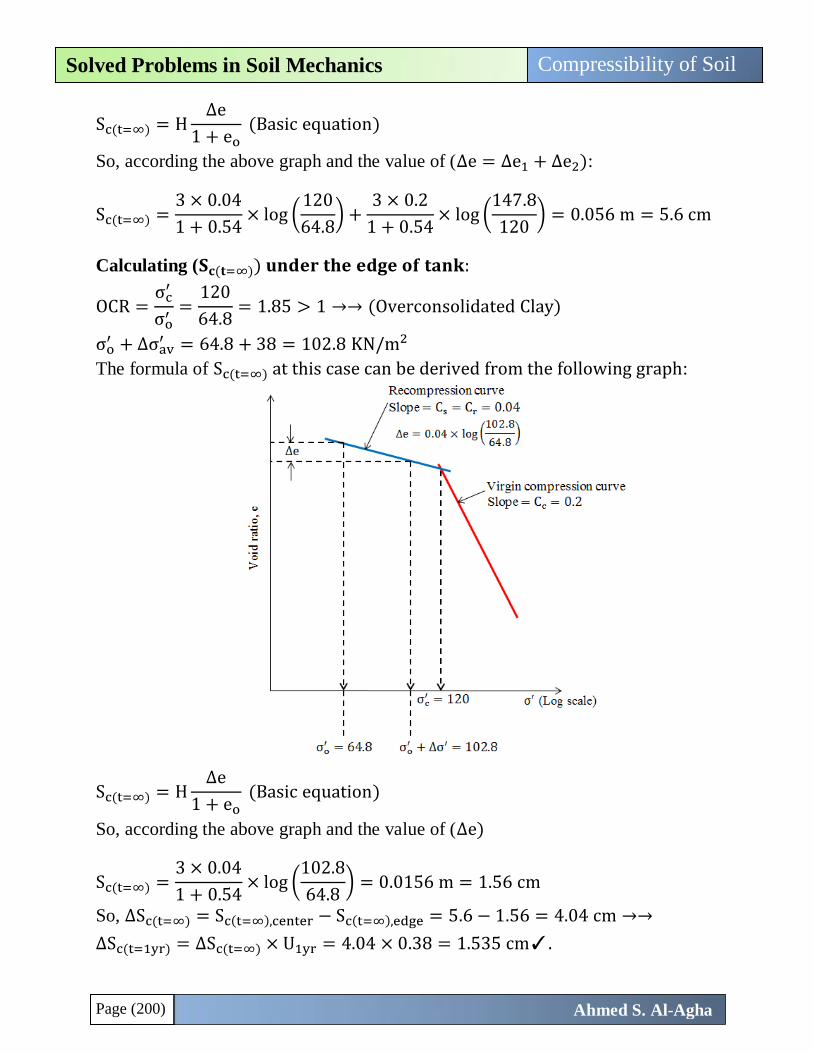
Page (200)
Compressibility of Soil Solved Problems in Soil Mechanics
Ahmed S. Al-Agha
Sc(t=∞) = H∆e
1 + eo (Basic equation)
So, according the above graph and the value of (∆e = ∆e1 + ∆e2):
Sc(t=∞) =3 × 0.04
1 + 0.54× log (
120
64.8) +
3 × 0.2
1 + 0.54× log (
147.8
120) = 0.056 m = 5.6 cm
Calculating (𝐒𝐜(𝐭=∞)) 𝐮𝐧𝐝𝐞𝐫 𝐭𝐡𝐞 𝐞𝐝𝐠𝐞 𝐨𝐟 𝐭𝐚𝐧𝐤:
OCR =σc
′
σo′ =
120
64.8= 1.85 > 1 →→ (Overconsolidated Clay)
σo′ + ∆σav
′ = 64.8 + 38 = 102.8 KN/m2
The formula of Sc(t=∞) at this case can be derived from the following graph:
Sc(t=∞) = H∆e
1 + eo (Basic equation)
So, according the above graph and the value of (∆e)
Sc(t=∞) =3 × 0.04
1 + 0.54× log (
102.8
64.8) = 0.0156 m = 1.56 cm
So, ∆Sc(t=∞) = Sc(t=∞),center − Sc(t=∞),edge = 5.6 − 1.56 = 4.04 cm →→
∆Sc(t=1yr) = ∆Sc(t=∞) × U1yr = 4.04 × 0.38 = 1.535 cm✓.
Chapter (12)
Shear Strength of Soil
Page (202)
Shear Strength of Soil Solved Problems in Soil Mechanics
Ahmed S. Al-Agha
Introduction The shear strength of a soil mass is the internal resistance per unit area that the
soil mass can offer to resist failure and sliding along any plane inside it.
You should know that, the safety of any geotechnical structure is dependent on the
strength of the soil, so if the soil fails, the structure founded on it may collapse.
Therefore, engineers must understand the nature of shearing resistance in order to
analyze soil stability problems such as:
Bearing capacity.
Slope stability.
Lateral pressure on retaining structures.
What Is Shear Failure??
( مماسيه shear stressesنه سيتولد عليها قوى واجهادات )عندما تتعرض التربة لقوى خارجية )رأسية( فإ
بين الحبيبات تحاول جعل جزء من التربة ينفصل أو ينزلق عن باقي كتلة التربة.
ولكل نوع من أنواع التربة قدرة محددة على مقاومة حدوث مثل هذا االنهيار حيث أن أقصى قيمة لهذه
Shear Strength (𝛕𝐟المقاومة تعرف ب = 𝛕𝐦𝐚𝐱@𝐟𝐚𝐢𝐥𝐮𝐫𝐞) .
( shear stressesفي التربة عندما تصل اجهادات القص المتولدة داخل التربة ) shear failureويحدث ال
أو تتجاوزها. shear strengthإلى قيمة ال
كما يلي: shear strengthوبالتالي يمكن تعريف ال
فيها انهيار بالقص )انزالق أجزاء التربة على بعضها(. هو اٌقصى اجهاد قص يتولد داخل التربة ويسبب
أسباب قدرة التربة على مقاومة حدوث قص بها:
التداخل بين حبيبات التربة. .1
( ويكون عادة في حالة التربة الرملية internal frictionاالحتكاك الداخلي بين الحبيبات الخشنة ) .2
(sandy soil or cohesionless soil.)
clayey soil or( ويكون عادة في التربة الطينية )Cohesionبين الحبيبات الناعمة )التماسك .3
cohesive soil.)
Mohr – Coulomb Failure Criterion ألي تربة حيث أن هذه المعادلة تعتبر shear strengthوضع هاذان العالمان المعادلة العامة لحساب ال
ن المعادلة كما يلي:معادلة خطية )معادلة خط مستقيم( حيث أ
τf = c + σf tanϕ
Where,
τf = shear strength of soil
Page (203)
Shear Strength of Soil Solved Problems in Soil Mechanics
Ahmed S. Al-Agha
c = cohesion = التماسك بين حبيبات التربة الناعمة
σf = normal stress on the failure plane
= االجهاد المتولد داخل كتلة التربة وهو عمودي على مستوى االنهيار
ϕ = angle of internal friction
tanϕ = معامل االحتكاك بين حبيبات التربة الخشنة
Shear strength for different types of soil
Sandy soil:
تصنف التربة الرملية على أنها تربة خشنة وبالتالي يوجد احتكاك داخلي بين حبيباتها، ولكن ال يوجد التصاق
ت التربة الناعمةبين حبيباتها ألنها تربة خشنة وااللتصاق يكون بين حبيبا
So, for sandy soil:
c = 0.0
→ τf = σf tanϕ
Normal Consolidated Clay:
For normal consolidated clay, the value of cohesion (c) can be approximated at
zero.
ا النوع من ( أن هذ11على الرغم من أن حبيبات هذه التربة ناعمة نوعا ما، لكن من المعروف )من شبتر
التربة يتعرض ألحمال كبيرة وبالتالي فإن أغلب كميات المياه التي بداخلها سوف تخرج، وبالتالي تفقد
التماسك بين حبيباتها تقريبا وتكون أقرب للحالة الخشنة، لذلك يمكن اعتبار قيمة التماسك بهذا النوع من
ي بين حبيباتها.التربة، وتشبيهها بالتربة الرملية حيث يكون احتكاك داخل
So, for normal consolidated clay:
c = 0.0
→ τf = σf tanϕ
Clayey Soil:
تصنف التربة الطينية على أنها تربة ناعمة، بالتالي يوجد التصاق بين حبيباتها، ولكن ال يوجد احتكاك داخلي
نة.بين حبيباتها ألنها تربة ناعمة واالحتكاك يحدث بين حبيبات التربة الخش
So, for clayey soil:
ϕ = 0.0
→ τf = c
OverConsolidated Clay:
أن األحمال التي يتم تطبيقها على 11يصنف هذا النوع من التربة على أنه تربة ناعمة، حيث نتذكر من شبتر
بيباتها أي هذا النوع ليست كبيرة جدا، بالتالي يبقى التماسك بين حبيباتها الناعمة، ولكن ال يوجد احتكاك بين ح
يتم التعامل معها تماما مثل التربة الطينية.
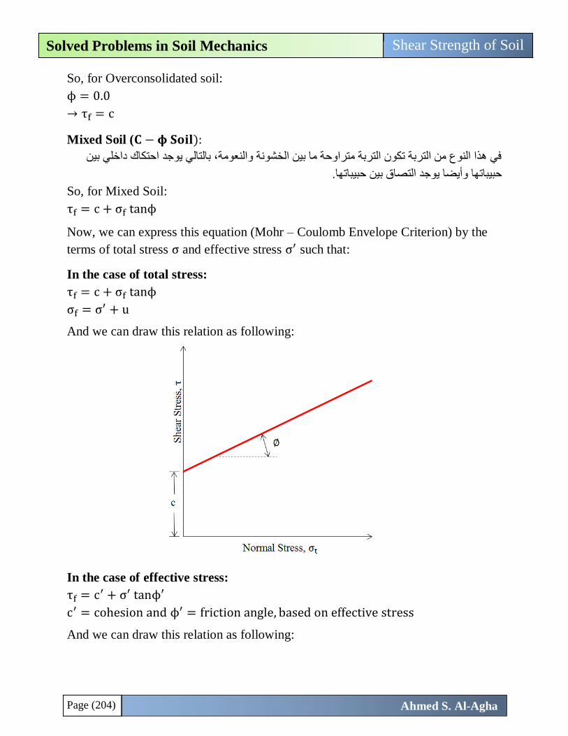
Page (204)
Shear Strength of Soil Solved Problems in Soil Mechanics
Ahmed S. Al-Agha
So, for Overconsolidated soil:
ϕ = 0.0
→ τf = c
Mixed Soil (𝐂 − 𝛟 𝐒𝐨𝐢𝐥):
في هذا النوع من التربة تكون التربة متراوحة ما بين الخشونة والنعومة، بالتالي يوجد احتكاك داخلي بين
ين حبيباتها.حبيباتها وأيضا يوجد التصاق ب
So, for Mixed Soil:
τf = c + σf tanϕ
Now, we can express this equation (Mohr – Coulomb Envelope Criterion) by the
terms of total stress σ and effective stress σ′ such that:
In the case of total stress:
τf = c + σf tanϕ
σf = σ′ + u
And we can draw this relation as following:
In the case of effective stress:
τf = c′ + σ′ tanϕ′
c′ = cohesion and ϕ′ = friction angle, based on effective stress
And we can draw this relation as following:
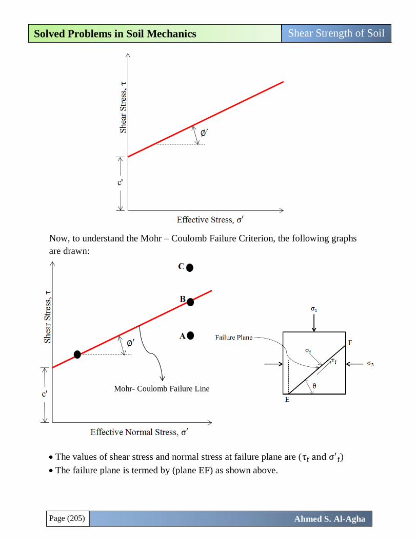
Page (205)
Shear Strength of Soil Solved Problems in Soil Mechanics
Ahmed S. Al-Agha
Now, to understand the Mohr – Coulomb Failure Criterion, the following graphs
are drawn:
The values of shear stress and normal stress at failure plane are (τf and σ′
f)
The failure plane is termed by (plane EF) as shown above.
Mohr- Coulomb Failure Line
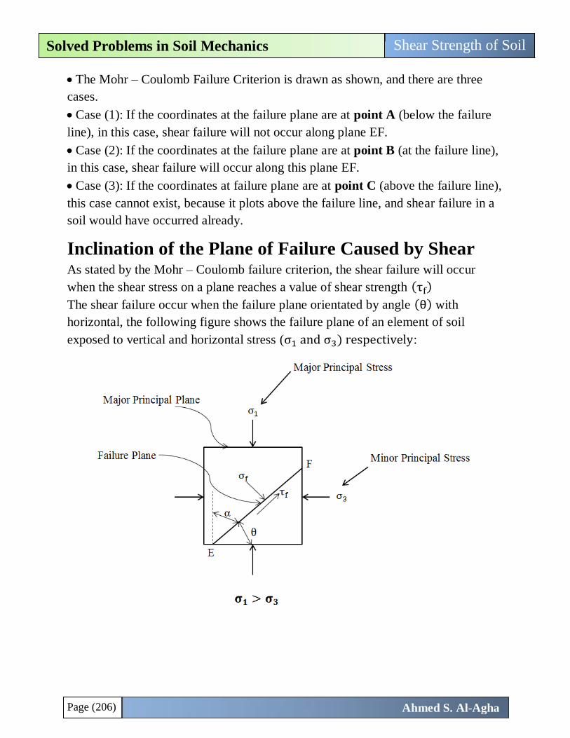
Page (206)
Shear Strength of Soil Solved Problems in Soil Mechanics
Ahmed S. Al-Agha
The Mohr – Coulomb Failure Criterion is drawn as shown, and there are three
cases.
Case (1): If the coordinates at the failure plane are at point A (below the failure
line), in this case, shear failure will not occur along plane EF.
Case (2): If the coordinates at the failure plane are at point B (at the failure line),
in this case, shear failure will occur along this plane EF.
Case (3): If the coordinates at failure plane are at point C (above the failure line),
this case cannot exist, because it plots above the failure line, and shear failure in a
soil would have occurred already.
Inclination of the Plane of Failure Caused by Shear
As stated by the Mohr – Coulomb failure criterion, the shear failure will occur
when the shear stress on a plane reaches a value of shear strength (τf)
The shear failure occur when the failure plane orientated by angle (θ) with
horizontal, the following figure shows the failure plane of an element of soil
exposed to vertical and horizontal stress (σ1 and σ3) respectively:
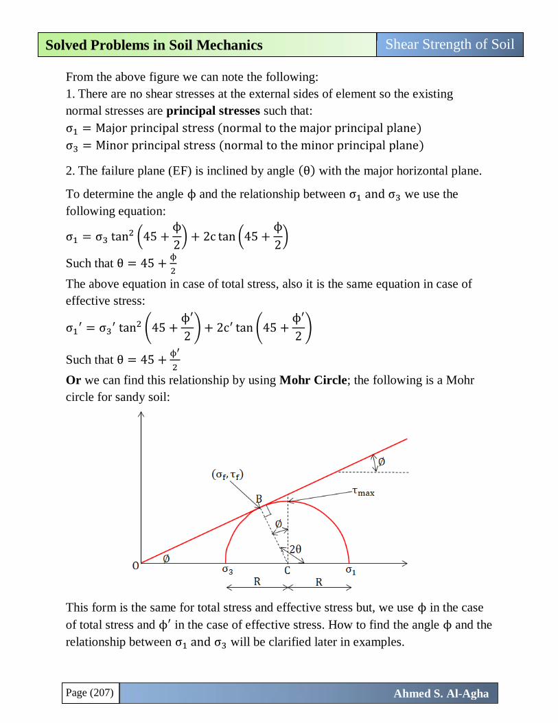
Page (207)
Shear Strength of Soil Solved Problems in Soil Mechanics
Ahmed S. Al-Agha
From the above figure we can note the following:
1. There are no shear stresses at the external sides of element so the existing
normal stresses are principal stresses such that:
σ1 = Major principal stress (normal to the major principal plane)
σ3 = Minor principal stress (normal to the minor principal plane)
2. The failure plane (EF) is inclined by angle (θ) with the major horizontal plane.
To determine the angle ϕ and the relationship between σ1 and σ3 we use the
following equation:
σ1 = σ3 tan2 (45 +ϕ
2) + 2c tan (45 +
ϕ
2)
Such that θ = 45 +ϕ
2
The above equation in case of total stress, also it is the same equation in case of
effective stress:
σ1′ = σ3
′ tan2 (45 +ϕ′
2) + 2c′ tan (45 +
ϕ′
2)
Such that θ = 45 +ϕ′
2
Or we can find this relationship by using Mohr Circle; the following is a Mohr
circle for sandy soil:
This form is the same for total stress and effective stress but, we use ϕ in the case
of total stress and ϕ′ in the case of effective stress. How to find the angle ϕ and the
relationship between σ1 and σ3 will be clarified later in examples.
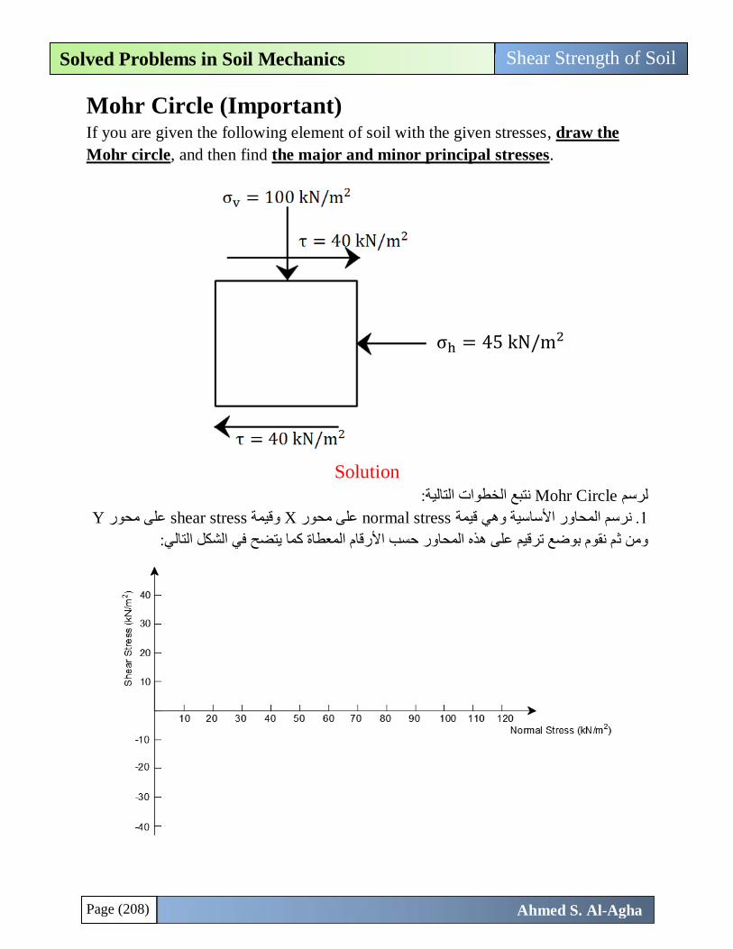
Page (208)
Shear Strength of Soil Solved Problems in Soil Mechanics
Ahmed S. Al-Agha
Mohr Circle (Important) If you are given the following element of soil with the given stresses, draw the
Mohr circle, and then find the major and minor principal stresses.
Solution
نتبع الخطوات التالية: Mohr Circleلرسم
Yعلى محور shear stressوقيمة Xعلى محور normal stressنرسم المحاور األساسية وهي قيمة .1
م نقوم بوضع ترقيم على هذه المحاور حسب األرقام المعطاة كما يتضح في الشكل التالي:ثومن
σh = 45 kN/m2
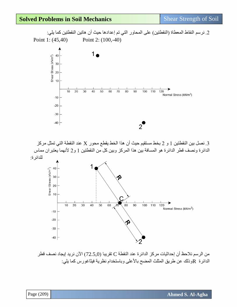
Page (209)
Shear Strength of Soil Solved Problems in Soil Mechanics
Ahmed S. Al-Agha
النقاط المعطاة )النقطتين( على المحاور التي تم إعدادها حيث أن هاتين النقطتين كما يلي: نرسم .2
Point 1: (45,40) Point 2: (100,-40)
عند النقطة التي تمثل مركز Xبخط مستقيم حيث أن هذا الخط يقطع محور 2و 1ن النقطتين نصل بي .3
ألنهما يعتبران مماس 2و 1ونصف قطر الدائرة هو المسافة بين هذا المركز وبين كل من النقطتين الدائرة
للدائرة:
( اآلن نريد إيجاد نصف قطر 72.5,0)تقريبا Cمن الرسم نالحظ أن إحداثيات مركز الدائرة عند النقطة
وذلك عن طريق المثلث المضح باألعلى وباستخدام نظرية فيثاغورس كما يلي: Rالدائرة
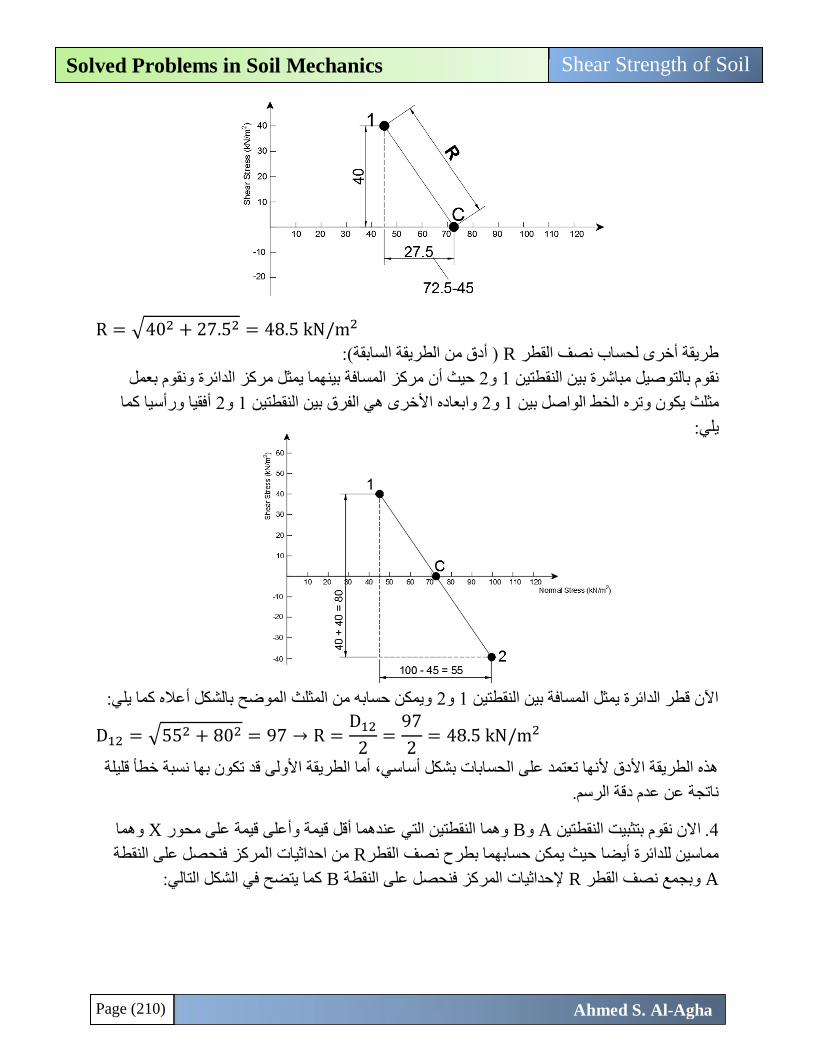
Page (210)
Shear Strength of Soil Solved Problems in Soil Mechanics
Ahmed S. Al-Agha
R = √402 + 27.52 = 48.5 kN/m2
) أدق من الطريقة السابقة(: Rطريقة أخرى لحساب نصف القطر
مركز المسافة بينهما يمثل مركز الدائرة ونقوم بعمل حيث أن 2و 1نقوم بالتوصيل مباشرة بين النقطتين
أفقيا ورأسيا كما 2و 1وابعاده األخرى هي الفرق بين النقطتين 2و 1يكون وتره الخط الواصل بين مثلث
يلي:
ي:ويمكن حسابه من المثلث الموضح بالشكل أعاله كما يل 2و 1اآلن قطر الدائرة يمثل المسافة بين النقطتين
D12 = √552 + 802 = 97 → R =D12
2=
97
2= 48.5 kN/m2
هذه الطريقة األدق ألنها تعتمد على الحسابات بشكل أساسي، أما الطريقة األولى قد تكون بها نسبة خطأ قليلة
ناتجة عن عدم دقة الرسم.
وهما Xوأعلى قيمة على محور وهما النقطتين التي عندهما أقل قيمة Bو Aاالن نقوم بتثبيت النقطتين .4
من احداثيات المركز فنحصل على النقطة Rحيث يمكن حسابهما بطرح نصف القطر مماسين للدائرة أيضا
A وبجمع نصف القطرR إلحداثيات المركز فنحصل على النقطةB :كما يتضح في الشكل التالي
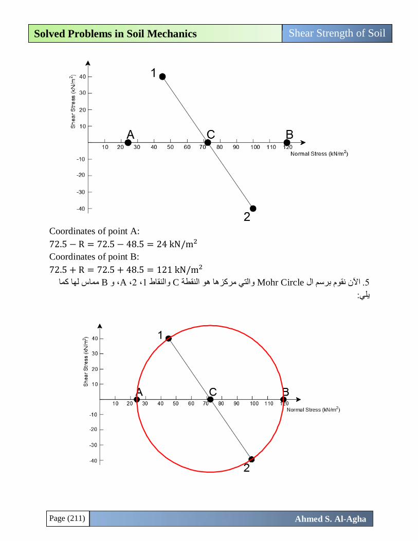
Page (211)
Shear Strength of Soil Solved Problems in Soil Mechanics
Ahmed S. Al-Agha
Coordinates of point A:
72.5 − R = 72.5 − 48.5 = 24 kN/m2
Coordinates of point B:
72.5 + R = 72.5 + 48.5 = 121 kN/m2
مماس لها كما B، و A، 2، 1والنقاط Cوالتي مركزها هو النقطة Mohr Circleاآلن نقوم برسم ال .5
يلي:
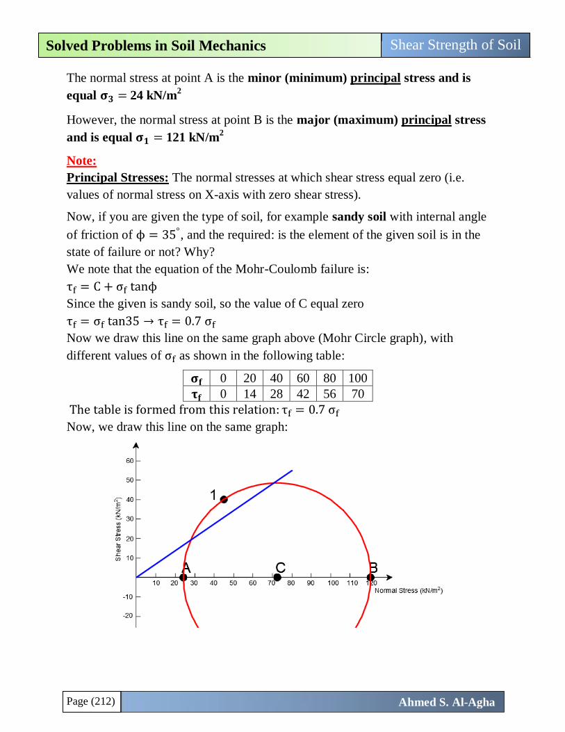
Page (212)
Shear Strength of Soil Solved Problems in Soil Mechanics
Ahmed S. Al-Agha
The normal stress at point A is the minor (minimum) principal stress and is
equal 𝛔𝟑 = 24 kN/m2
However, the normal stress at point B is the major (maximum) principal stress
and is equal 𝛔𝟏 = 121 kN/m2
Note:
Principal Stresses: The normal stresses at which shear stress equal zero (i.e.
values of normal stress on X-axis with zero shear stress).
Now, if you are given the type of soil, for example sandy soil with internal angle
of friction of ϕ = 35°, and the required: is the element of the given soil is in the
state of failure or not? Why?
We note that the equation of the Mohr-Coulomb failure is:
τf = C + σf tanϕ
Since the given is sandy soil, so the value of C equal zero
τf = σf tan35 → τf = 0.7 σf
Now we draw this line on the same graph above (Mohr Circle graph), with
different values of σf as shown in the following table:
𝛔𝐟 0 20 40 60 80 100
𝛕𝐟 0 14 28 42 56 70
The table is formed from this relation: τf = 0.7 σf
Now, we draw this line on the same graph:
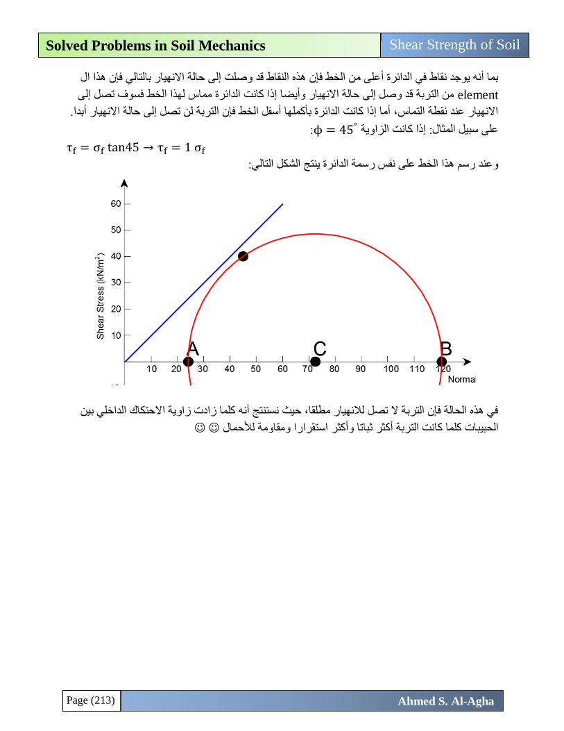
Page (213)
Shear Strength of Soil Solved Problems in Soil Mechanics
Ahmed S. Al-Agha
ي فإن هذا البما أنه يوجد نقاط في الدائرة أعلى من الخط فإن هذه النقاط قد وصلت إلى حالة االنهيار بالتال
element من التربة قد وصل إلى حالة االنهيار وأيضا إذا كانت الدائرة مماس لهذا الخط فسوف تصل إلى
االنهيار عند نقطة التماس، أما إذا كانت الدائرة بأكملها أسفل الخط فإن التربة لن تصل إلى حالة االنهيار أبدا.
ϕعلى سبيل المثال: إذا كانت الزاوية = 45°:
τf = σf tan45 → τf = 1 σf
وعند رسم هذا الخط على نفس رسمة الدائرة ينتج الشكل التالي:
في هذه الحالة فإن التربة ال تصل لالنهيار مطلقا، حيث نستنتج أنه كلما زادت زاوية االحتكاك الداخلي بين
ومقاومة لألحمال الحبيبات كلما كانت التربة أكثر ثباتا وأكثر استقرارا
Page (214)
Shear Strength of Soil Solved Problems in Soil Mechanics
Ahmed S. Al-Agha
Laboratory Tests for Determination of Shear Strength
Parameters There are several laboratory methods available to determine the shear strength
parameters (i.e.,c, ϕ, c′, ϕ′) of various soil specimens in the laboratory. The most
important two tests are:
1. Direct Shear Test.
2. Triaxial Test.
Direct Shear Test This test has been discussed completely in the laboratory, so we will not discuss it
here.
Triaxial Test Triaxial shear test is one of the most reliable methods available for determining
shear strength parameters. It is used widely for research and conventional testing.
The following three standard types of triaxial tests generally are conducted:
1. Consolidated – drained test (CD test).
2. Consolidated – undrained test (CU test).
3. Unconsolidated – undrained test (UU test).
We will discuss completely the first two types (CD and CU) and the third type, you
can read it from your text book Page 461.
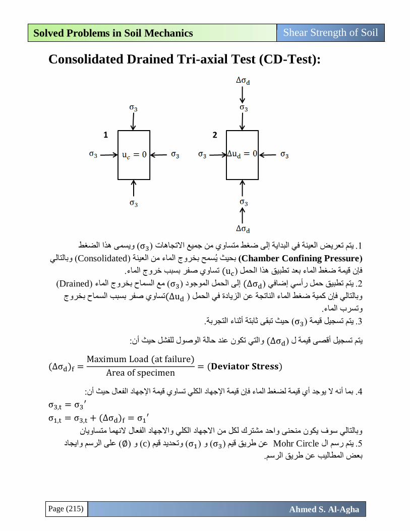
Page (215)
Shear Strength of Soil Solved Problems in Soil Mechanics
Ahmed S. Al-Agha
Consolidated Drained Tri-axial Test (CD-Test):
ويسمى هذا الضغط (σ3)ض العينة في البداية إلى ضغط متساوي من جميع االتجاهات يتم تعري .1
(Chamber Confining Pressure) ( بحيث ي سمح بخروج الماء من العينةConsolidated وبالتالي )
تساوي صفر بسبب خروج الماء. uc)فإن قيمة ضغط الماء بعد تطبيق هذا الحمل )
( Drained( مع السماح بخروج الماء )σ3إلى الحمل الموجود ) σd∆))إضافي يتم تطبيق حمل رأسي .2
تساوي صفر بسبب السماح بخروج ud∆))وبالتالي فإن كمية ضغط الماء الناتجة عن الزيادة في الحمل
وتسرب الماء.
حيث تبقى ثابتة أثناء التجربة. (σ3)يتم تسجيل قيمة .3
تكون عند حالة الوصول للفشل حيث أن:والتي σd∆)يتم تسجيل أقصى قيمة ل )
(∆σd)f =Maximum Load (at failure)
Area of specimen= (𝐃𝐞𝐯𝐢𝐚𝐭𝐨𝐫 𝐒𝐭𝐫𝐞𝐬𝐬)
:بما أنه ال يوجد أي قيمة لضغط الماء فإن قيمة اإلجهاد الكلي تساوي قيمة اإلجهاد الفعال حيث أن .4
σ3,t = σ3′
σ1,t = σ3,t + (∆σd)f = σ1′
وبالتالي سوف يكون منحنى واحد مشترك لكل من االجهاد الكلي واالجهاد الفعال النهما متساويان
( على الرسم وايجاد ∅( و )cوتحديد قيم ) (σ1)و (σ3)عن طريق قيم Mohr Circle يتم رسم ال .5
بعض المطاليب عن طريق الرسم.
1 2
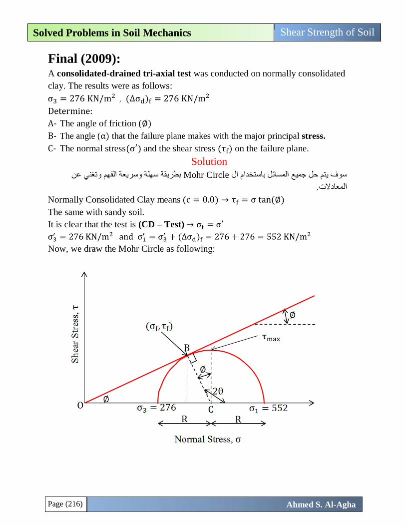
Page (216)
Shear Strength of Soil Solved Problems in Soil Mechanics
Ahmed S. Al-Agha
Final (2009): A consolidated-drained tri-axial test was conducted on normally consolidated
clay. The results were as follows:
σ3 = 276 KN/m2 , (∆σd)f = 276 KN/m2
Determine:
A- The angle of friction (∅)
B- The angle (α) that the failure plane makes with the major principal stress.
C- The normal stress(σ′) and the shear stress (τf) on the failure plane.
Solution
بطريقة سهلة وسريعة الفهم وتغني عن Mohr Circleسوف يتم حل جميع المسائل باستخدام ال
المعادالت.
Normally Consolidated Clay means (c = 0.0) → τf = σ tan (∅)
The same with sandy soil.
It is clear that the test is (CD – Test) → σt = σ′
σ3′ = 276 KN/m2 and σ1
′ = σ3′ + (∆σd)f = 276 + 276 = 552 KN/m2
Now, we draw the Mohr Circle as following:
A
τmax
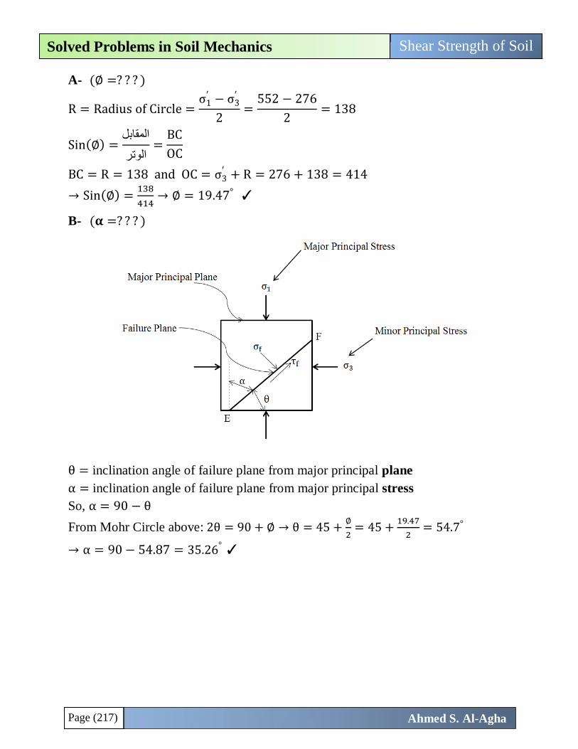
Page (217)
Shear Strength of Soil Solved Problems in Soil Mechanics
Ahmed S. Al-Agha
A- (∅ =? ? ? )
R = Radius of Circle =σ1
′ − σ3′
2=
552 − 276
2= 138
Sin(∅) =المقابل
الوتر=
BC
OC
BC = R = 138 and OC = σ3′ + R = 276 + 138 = 414
→ Sin(∅) =138
414→ ∅ = 19.47° ✓
B- (𝛂 =? ? ? )
θ = inclination angle of failure plane from major principal plane
α = inclination angle of failure plane from major principal stress
So, α = 90 − θ
From Mohr Circle above: 2θ = 90 + ∅ → θ = 45 +∅
2= 45 +
19.47
2= 54.7°
→ α = 90 − 54.87 = 35.26° ✓
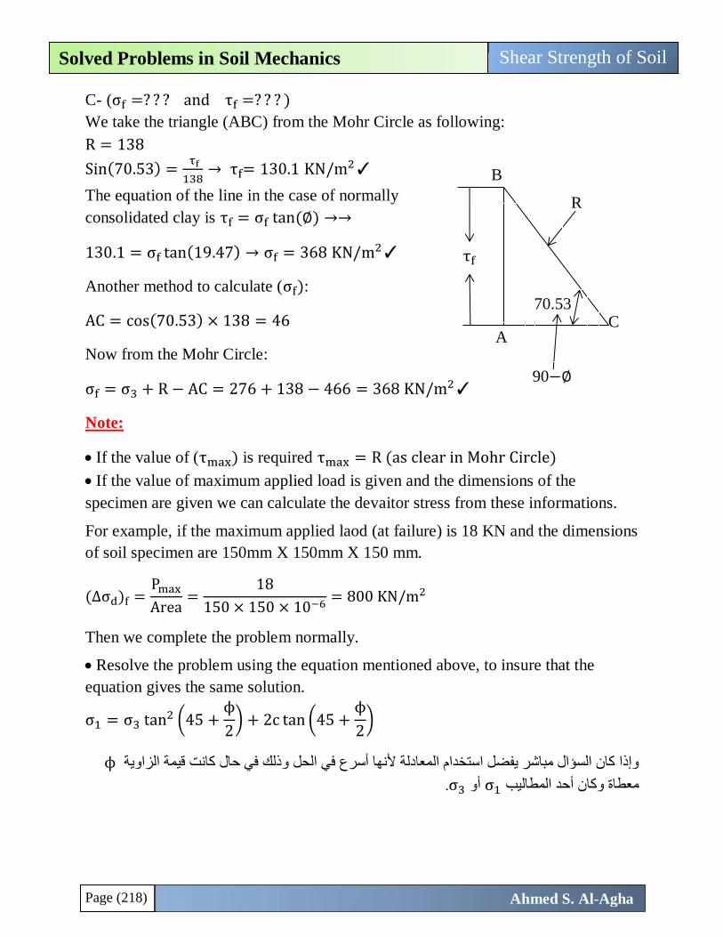
Page (218)
Shear Strength of Soil Solved Problems in Soil Mechanics
Ahmed S. Al-Agha
C- (σf =? ? ? and τf =? ? ? )
We take the triangle (ABC) from the Mohr Circle as following:
R = 138
Sin(70.53) = τf
138→ τf= 130.1 KN/m2✓
The equation of the line in the case of normally
consolidated clay is τf = σf tan (∅) →→
130.1 = σf tan(19.47) → σf = 368 KN/m2✓
Another method to calculate (σf):
AC = cos(70.53) × 138 = 46
Now from the Mohr Circle:
σf = σ3 + R − AC = 276 + 138 − 466 = 368 KN/m2✓
Note:
If the value of (τmax) is required τmax = R (as clear in Mohr Circle)
If the value of maximum applied load is given and the dimensions of the
specimen are given we can calculate the devaitor stress from these informations.
For example, if the maximum applied laod (at failure) is 18 KN and the dimensions
of soil specimen are 150mm X 150mm X 150 mm.
(∆σd)f =Pmax
Area=
18
150 × 150 × 10−6= 800 KN/m2
Then we complete the problem normally.
Resolve the problem using the equation mentioned above, to insure that the
equation gives the same solution.
σ1 = σ3 tan2 (45 +ϕ
2) + 2c tan (45 +
ϕ
2)
ϕالزاوية وذلك في حال كانت قيمة وإذا كان السؤال مباشر يفضل استخدام المعادلة ألنها أسرع في الحل
.σ3 أو σ1معطاة وكان أحد المطاليب
A
B
C
τf
R
70.53
90−∅
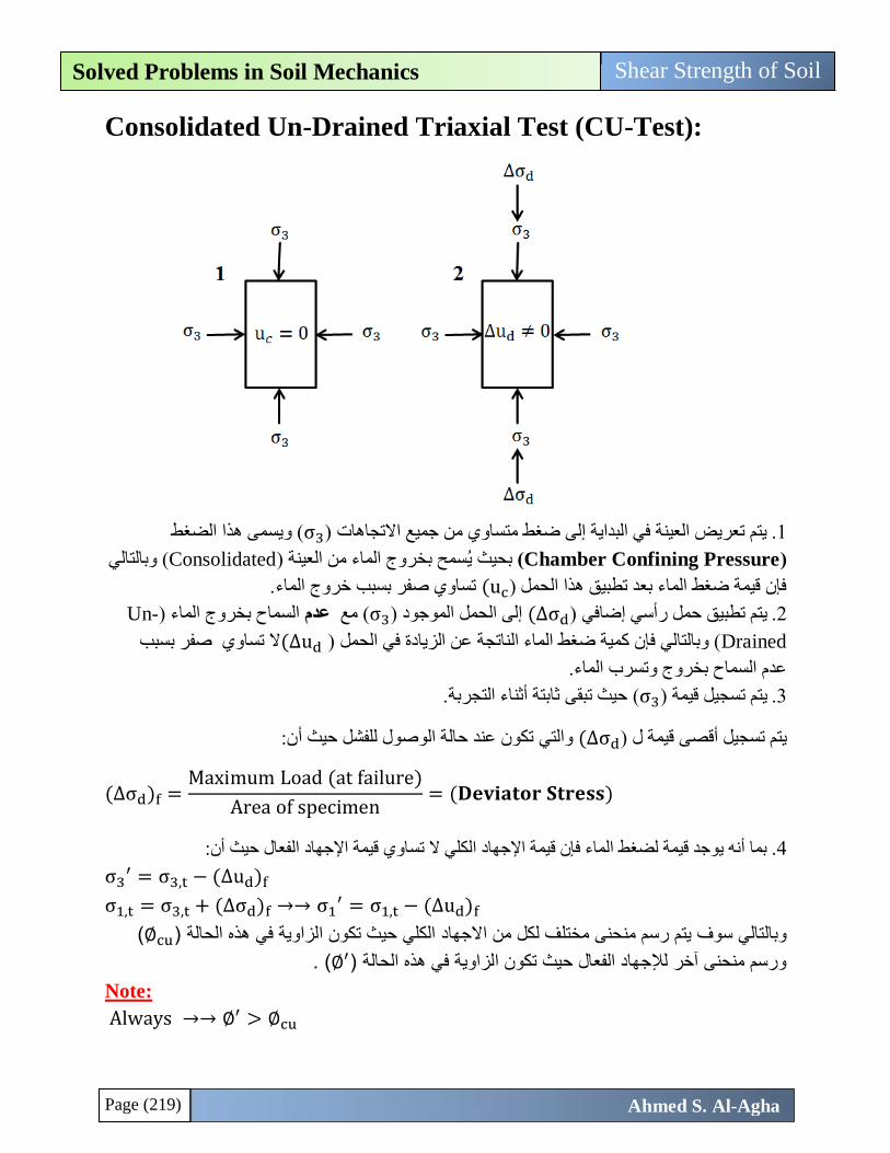
Page (219)
Shear Strength of Soil Solved Problems in Soil Mechanics
Ahmed S. Al-Agha
Consolidated Un-Drained Triaxial Test (CU-Test):
( ويسمى هذا الضغط σ3يتم تعريض العينة في البداية إلى ضغط متساوي من جميع االتجاهات ) .1
(Chamber Confining Pressure) سمح بخروج الماء من البحيث ي( عينةConsolidated وبالتالي )
تساوي صفر بسبب خروج الماء. uc)فإن قيمة ضغط الماء بعد تطبيق هذا الحمل )
-Unالسماح بخروج الماء ) عدم( مع σ3إلى الحمل الموجود ) σd∆))يتم تطبيق حمل رأسي إضافي .2
Drainedمل ( وبالتالي فإن كمية ضغط الماء الناتجة عن الزيادة في الح((∆ud ال تساوي صفر بسبب
عدم السماح بخروج وتسرب الماء.
حيث تبقى ثابتة أثناء التجربة. (σ3)يتم تسجيل قيمة .3
تكون عند حالة الوصول للفشل حيث أن:والتي σd∆)يتم تسجيل أقصى قيمة ل )
(∆σd)f =Maximum Load (at failure)
Area of specimen= (𝐃𝐞𝐯𝐢𝐚𝐭𝐨𝐫 𝐒𝐭𝐫𝐞𝐬𝐬)
:قيمة اإلجهاد الفعال حيث أن ال تساوي بما أنه يوجد قيمة لضغط الماء فإن قيمة اإلجهاد الكلي .4
σ3′ = σ3,t − (∆ud)f
σ1,t = σ3,t + (∆σd)f →→ σ1′ = σ1,t − (∆ud)f
(cu∅)حيث تكون الزاوية في هذه الحالة وبالتالي سوف يتم رسم منحنى مختلف لكل من االجهاد الكلي
( .′∅ورسم منحنى آخر لإلجهاد الفعال حيث تكون الزاوية في هذه الحالة )
Note:
Always →→ ∅′ > ∅cu
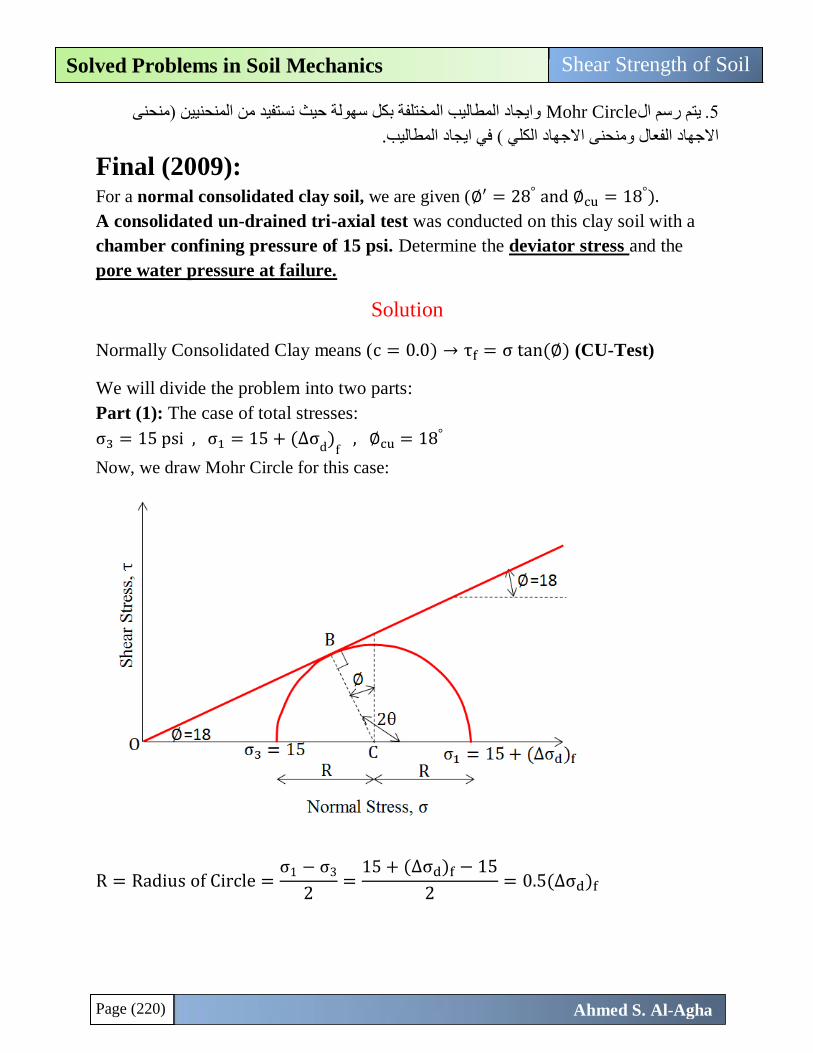
Page (220)
Shear Strength of Soil Solved Problems in Soil Mechanics
Ahmed S. Al-Agha
وايجاد المطاليب المختلفة بكل سهولة حيث نستفيد من المنحنيين )منحنى Mohr Circleيتم رسم ال .5
.هاد الكلي ( في ايجاد المطاليبجاالجهاد الفعال ومنحنى اال
Final (2009): For a normal consolidated clay soil, we are given (∅′ = 28° and ∅cu = 18°).
A consolidated un-drained tri-axial test was conducted on this clay soil with a
chamber confining pressure of 15 psi. Determine the deviator stress and the
pore water pressure at failure.
Solution
Normally Consolidated Clay means (c = 0.0) → τf = σ tan (∅) (CU-Test)
We will divide the problem into two parts:
Part (1): The case of total stresses:
σ3 = 15 psi , σ1 = 15 + (∆σd)
f , ∅cu = 18°
Now, we draw Mohr Circle for this case:
R = Radius of Circle =σ1 − σ3
2=
15 + (∆σd)f − 15
2= 0.5(∆σd)f
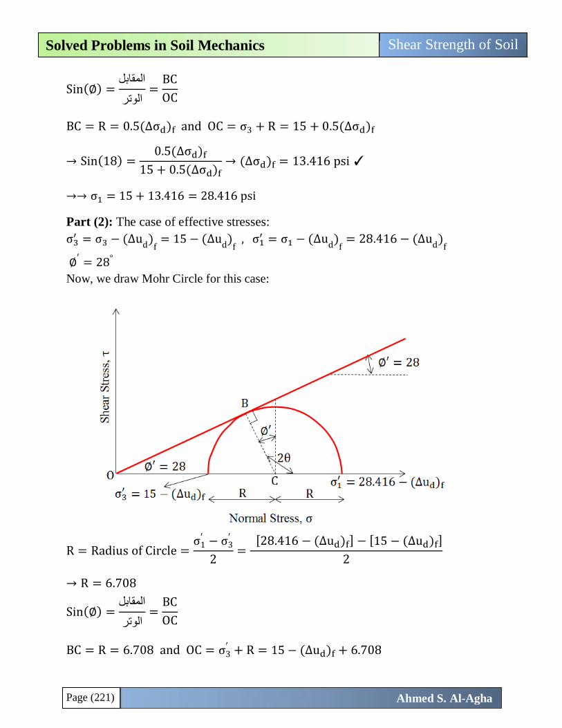
Page (221)
Shear Strength of Soil Solved Problems in Soil Mechanics
Ahmed S. Al-Agha
Sin(∅) =المقابل
الوتر=
BC
OC
BC = R = 0.5(∆σd)f and OC = σ3 + R = 15 + 0.5(∆σd)f
→ Sin(18) =0.5(∆σd)f
15 + 0.5(∆σd)f→ (∆σd)f = 13.416 psi ✓
→→ σ1 = 15 + 13.416 = 28.416 psi
Part (2): The case of effective stresses:
σ3′ = σ3 − (∆u
d)
f= 15 − (∆u
d)
f , σ1
′ = σ1 − (∆ud)
f= 28.416 − (∆u
d)
f
∅′ = 28°
Now, we draw Mohr Circle for this case:
R = Radius of Circle =σ1
′ − σ3′
2=
[28.416 − (∆ud)f] − [15 − (∆ud)f]
2
→ R = 6.708
Sin(∅) =المقابل
الوتر=
BC
OC
BC = R = 6.708 and OC = σ3′ + R = 15 − (∆ud)f + 6.708
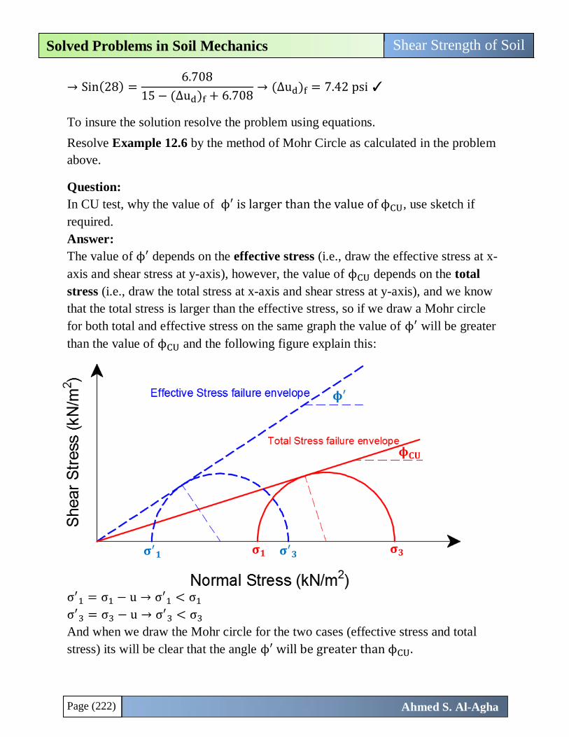
Page (222)
Shear Strength of Soil Solved Problems in Soil Mechanics
Ahmed S. Al-Agha
→ Sin(28) =6.708
15 − (∆ud)f + 6.708→ (∆ud)f = 7.42 psi ✓
To insure the solution resolve the problem using equations.
Resolve Example 12.6 by the method of Mohr Circle as calculated in the problem
above.
Question:
In CU test, why the value of ϕ′ is larger than the value of ϕCU, use sketch if
required.
Answer:
The value of ϕ′ depends on the effective stress (i.e., draw the effective stress at x-
axis and shear stress at y-axis), however, the value of ϕCU depends on the total
stress (i.e., draw the total stress at x-axis and shear stress at y-axis), and we know
that the total stress is larger than the effective stress, so if we draw a Mohr circle
for both total and effective stress on the same graph the value of ϕ′ will be greater
than the value of ϕCU and the following figure explain this:
σ′1 = σ1 − u → σ′
1 < σ1
σ′3 = σ3 − u → σ′
3 < σ3
And when we draw the Mohr circle for the two cases (effective stress and total
stress) its will be clear that the angle ϕ′ will be greater than ϕCU.
𝛔′𝟏
𝛔′𝟑 𝛔𝟏 𝛔𝟑
𝛟𝐂𝐔
𝛟′
𝛔′𝟑 𝛔𝟏 𝛔𝟑