Embed Size (px)
Citation preview


;
Microlensing Modelling with Nested
Sampling
Ashna SharanPhD Candidate
Supervisor: Dr. Nicholas Rattenbury
Department of Physics
University of Auckland

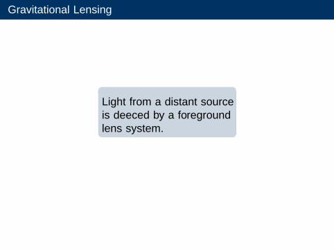
Gravitational Lensing
Light from a distant sourceis defleced by a foregroundlens system.
Multiple resolvable imagesform.
Gravitational Lensing
Light from a distant sourceis defleced by a foregroundlens system.
Multiple resolvable imagesform.
Gravitational Lensing
Light from a distant sourceis defleced by a foregroundlens system.
Multiple resolvable imagesform.

Gravitational Lensing
Light from a distant sourceis defleced by a foregroundlens system.
Multiple resolvable imagesform.
Gravitational Lensing
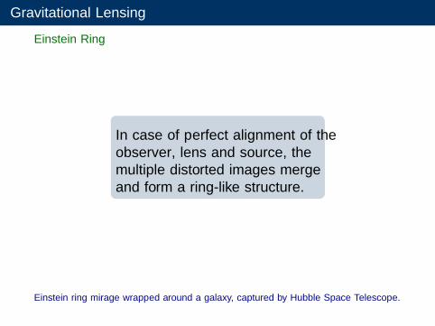
Einstein Ring
In case of perfect alignment of theobserver, lens and source, themultiple distorted images mergeand form a ring-like structure.
Einstein ring mirage wrapped around a galaxy, captured by Hubble Space Telescope.
Gravitational Lensing
Einstein Ring
In case of perfect alignment of theobserver, lens and source, themultiple distorted images mergeand form a ring-like structure.
Einstein ring mirage wrapped around a galaxy, captured by Hubble Space Telescope.
Gravitational Lensing
Microlensing
Lensing by single massive objects, forexample, a star, a stellar-binary, a starwith a planet companion.

Gravitational Lensing
Microlensing
Images too small(0.2-2milliarcseconds)to be resolved bytelescopes.
Due to therelative motion ofthe source andlens, we see abrightening of thesource star.
Microlensing - Single Lens
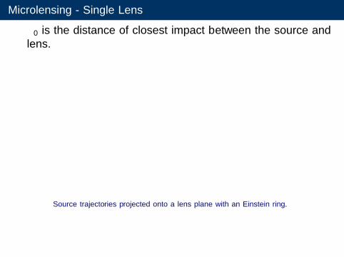
µ0 is the distance of closest impact between the source andlens.
Lens
θE
Source star
µ0µ(t)
Source trajectories projected onto a lens plane with an Einstein ring.
1
2
3
4
5
6
7
8
9
10
11
-1 -0.5 0 0.5 1
Amplification
Time, τ
µ0 = 0.1µ0 = 0.01
The smaller the µ0, the higher the peak of the lightcurve.

Microlensing - Single Lens
µ0 is the distance of closest impact between the source andlens.
Lens
θE
Source star
µ0µ(t)
Source trajectories projected onto a lens plane with an Einstein ring. 1
2
3
4
5
6
7
8
9
10
11
-1 -0.5 0 0.5 1
Amplification
Time, τ
µ0 = 0.1µ0 = 0.01
The smaller the µ0, the higher the peak of the lightcurve.

Microlensing - Binary Lens
Binary-lens light curves
Depending on the sourcelens configuration binary-lenslight curves can take manyforms.
0
2
4
6
8
10
12
14
16
6705 6710 6715 6720 6725 6730 6735 6740
Am
plifi
catio
n
Time (JD-245000)

Microlensing - Binary Lens
Binary-lens light curves
Depending on the sourcelens configuration binary-lenslight curves can take manyforms.
0
2
4
6
8
10
12
14
16
6705 6710 6715 6720 6725 6730 6735 6740
Am
plifi
catio
n
Time (JD-245000)

Microlensing - Binary Lens
Binary-lens light curves
Depending on the sourcelens configuration binary-lenslight curves can take manyforms.
0
2
4
6
8
10
12
14
16
6705 6710 6715 6720 6725 6730 6735 6740
Am
plifi
catio
n
Time (JD-245000)

Microlensing - Binary Lens
Binary-lens light curves
Depending on the sourcelens configuration binary-lenslight curves can take manyforms.
0
2
4
6
8
10
12
14
16
6705 6710 6715 6720 6725 6730 6735 6740
Am
plifi
catio
n
Time (JD-245000)

Microlensing Modelling Objectives
Need to find the best model to represent the observationalmicrolensing dataset.
� The Parameter Estimation Problem.
For a given model find a set of parameter values tobest-fit the data.
� The Model Selection Problem.
Choose between alternative models.

Microlensing Modelling Objectives
Need to find the best model to represent the observationalmicrolensing dataset.
� The Parameter Estimation Problem.
For a given model find a set of parameter values tobest-fit the data.
� The Model Selection Problem.
Choose between alternative models.

Microlensing Modelling Objectives
Need to find the best model to represent the observationalmicrolensing dataset.
� The Parameter Estimation Problem.
For a given model find a set of parameter values tobest-fit the data.
� The Model Selection Problem.
Choose between alternative models.

The Parameter Estimation Problem
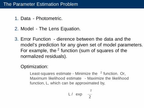
1. Data - Photometric.
2. Model - The Lens Equation.
3. Error Function - difference between the data and themodel’s prediction for any given set of model parameters.For example, the χ2 function (sum of squares of thenormalized residuals).
Optimization:
• Least-squares estimate - Minimize the χ2 function. Or,• Maximum likelihood estimate - Maximize the likelihood
function, L, which can be approximated by,
L ∝ exp
[−χ
2
2
]
The Parameter Estimation Problem
1. Data - Photometric.
2. Model - The Lens Equation.
3. Error Function - difference between the data and themodel’s prediction for any given set of model parameters.For example, the χ2 function (sum of squares of thenormalized residuals).
Optimization:
• Least-squares estimate - Minimize the χ2 function. Or,• Maximum likelihood estimate - Maximize the likelihood
function, L, which can be approximated by,
L ∝ exp
[−χ
2
2
]
The Data - Photometric
MOA, OGLE and KMTNet microlensing groups monitorhundreds of millions of stars in the Galactic Bulge.
Microlensing photometric data is obtained via DifferenceImage Analysis (DIA).

The Data - Photometric
More datasets from follow-up groups with their narrow fieldtelescopes.

The Model - Lens Equation
Maps image positions to source positions.
We know the source positions and need tofind the image positions to compute the
amplifications.
Amplification is the area of the images relativeto the area of the source.
Microlensing Modelling Challenges
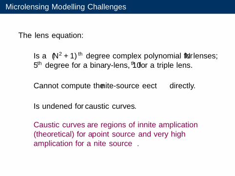
The lens equation:
Is a (N2 + 1)th degree complex polynomial for N lenses;5th degree for a binary-lens, 10th for a triple lens.
Cannot compute the finite-source effect directly.
Is undefined for caustic curves.
Caustic curves are regions of infinite amplification(theoretical) for a point source and very highamplification for a finite source.
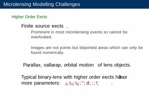
Microlensing Modelling Challenges
Higher Order Effects
Finite source effects.• Prominent in most microlensing events so cannot be
overlooked.
• Images are not points but disjointed areas which can only befound numerically.
Parallax, xallarap, orbital motion of lens objects.
Typical binary-lens with higher order effects has 9 ormore parameters: µ0, t0, tE , ε, d , α, ρ, ω, π .
Numerical solutions required!
Microlensing Modelling Code for Binary-lens System
GPU-accelerated binary-lens modelling code developed byJoe Ling, Massey University.
Magnification Map Technique
Dynamic Light Curve Engine*.
* Recently acquired from Joe.
Microlensing Modelling Code for Binary-lens System
GPU-accelerated binary-lens modelling code developed byJoe Ling, Massey University.
Magnification Map Technique
Dynamic Light Curve Engine*.
* Recently acquired from Joe.
Microlensing Modelling Code for Binary-lens System
GPU-accelerated binary-lens modelling code developed byJoe Ling, Massey University.
Magnification Map Technique
Dynamic Light Curve Engine*.
* Recently acquired from Joe.

Magnification Map
ε = 0.57, d = 0.9
Magnification maps are2-D array of solutionsto the lens equation.
Represents theparameter space {ε, d}.
Each pixel representsthe amplification ofthe source star at apoint in time.

Magnification Map Caustic Curve Patterns
Single Lens
The caustic is a point (the position of the lens).
ε = 0, d = 0Brighter color - higher amplification

Magnification Map Caustic Curve Patterns
Binary Lenses
The caustic curve patterns are more complicated.
ε = 0.5, d = 0.5
ε = 0.1, d = 2.0

Magnification Map Caustic Curve Patterns
Binary Lenses
The caustic curve patterns are more complicated.
ε = 0.5, d = 0.5
ε = 0.1, d = 2.0
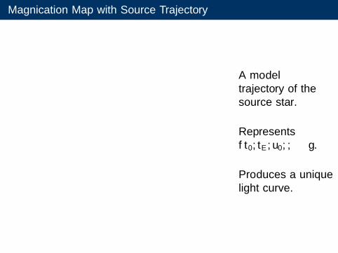
Magnification Map with Source Trajectory
A modeltrajectory of thesource star.
Represents{t0, tE , u0, α, ρ }.
Produces a uniquelight curve.

Magnification Map Generation - Inverse Ray Shooting
Billions of rays are shot backwards from the observer, throughthe lens onto the source plane.

Magnification Map Generation -Inverse Ray Shooting
Image Area Calculation
Lens plane is divided into a rectangular grid and rays shotfrom the 4 corners of each grid cell.
Image Credit: (Ling,2013)

Magnification Map Generation - Inverse Ray Shooting
Billions of rays are shot evenly from image area onto the sourceplane to determine the magnification of each of its pixel.
Image Credit: (Ling,2013)

Magnification Maps - Advantages
Finite source amplification can be computed directly byintegrating the source area on the magnification map.
Amplifications on caustic curve regions can be determined.

Caustic Curve Diagrams and Finite Source Effect
ε = 0.5, d = 0.5ρ = 0.001
Source crosses caustic curve at two points.

Caustic Curve Diagrams and Finite Source Effect
ε = 0.5, d = 0.5ρ = 0.001
Source crosses caustic curve at two points.

Caustic Curve Diagrams and Finite Source Effect
ε = 0.5, d = 0.5ρ = 0.02
Finite source effect - peaks appear washed out.

Caustic Curve Diagrams and Finite Source Effect
ε = 0.5, d = 0.5ρ = 0.02
Finite source effect - peaks appear washed out.

Magnification Maps - Advantages
Multiple light curves can be extracted from the samemagnification map.
α
µ0
1
Light curves corresponding to the source trajectories.

Magnification Maps - Advantages
Multiple light curves can be extracted from the samemagnification map.
α
µ0
1
Light curves corresponding to the source trajectories.

Magnification Map Technique
Grid search coupled with downhill simplexoptimization method.
Hundreds of thousands of light curves are extracted fromthousands of magnification maps to find rough initialmodels.
However, Magnification Map Technique cannot be usedwhen we want to:
• Optimize ε and d as free parameters during a Markov ChainMonte Carlo (MCMC) run.
• Account for orbital motion whereby projected distance, dchanges for each source position in time.
→ Dynamic Light Curve Engine.

Dynamic Light-Curve Engine
Computes the amplification value “on the fly”;bypassing magnification map generation.
“Image-centred” inverse ray shooting.The difference: rays are shot to the source star disk,
not to entire source plane.
MCMC optmization is used for finding more accuratemodels.

Dynamic Light-Curve Engine
Computes the amplification value “on the fly”;bypassing magnification map generation.
“Image-centred” inverse ray shooting.The difference: rays are shot to the source star disk,
not to entire source plane.
MCMC optmization is used for finding more accuratemodels.

Dynamic Light-Curve Engine
Computes the amplification value “on the fly”;bypassing magnification map generation.
“Image-centred” inverse ray shooting.The difference: rays are shot to the source star disk,
not to entire source plane.
MCMC optmization is used for finding more accuratemodels.

Dynamic Light Curve Engine: Image-centred IRS
Image Area Calculation
Solve complex polynomial to find point image positions(active cells).Recursively check if the neighbouring cells are active.
Image Credit: (Ling,2013)
Dynamic Light Curve Engine: Image-centred IRS
Shoot equal density of rays from the image area foreach source position in time .Relative amplification - number of collected rays
inside the source star.

Microlensing Modelling Objectives
X The Parameter Estimation Problem.
• Magnification Map Technique with Grid Search and DownhillSimplex.
• Dynamic Light Curve Engine with MCMC.
� The Model Selection Problem?

Microlensing Modelling Objectives
X The Parameter Estimation Problem.
• Magnification Map Technique with Grid Search and DownhillSimplex.
• Dynamic Light Curve Engine with MCMC.
� The Model Selection Problem?

The Microlensing Model Selection Problem
Choose between multiple competing models with comparableχ2 values.
Two different models specified by different number ofparameters:
• Binary lens or triple lens?
• Static binary-lens or with orbital motion?
One specific model produces two comparable modeswith different sets of parameter values.

Example 1. - Microlensing Model Selection Problem
Solution 1: A star and planet lens system with orbitalmotion.
Solution 2: Static binary star lens system.
Example 2. - Microlensing Model Selection Problem
OGLE-2004-BLG-490 : Binary-lens model with 7 parameters
ε = 0.04, d = 1.43, ρ = 0.001, α = 6.02, t0 = 3224.0, tE = 14.9, µ0 = 0.22

Example 2. - Microlensing Model Selection Problem
OGLE-2004-BLG-490 : Binary-lens model with 7 parameters
ε = 0.11, d = 1.71, ρ = 0.08, α = −0.01, t0 = 3225.3, tE = 12.7, µ0 = 0.32
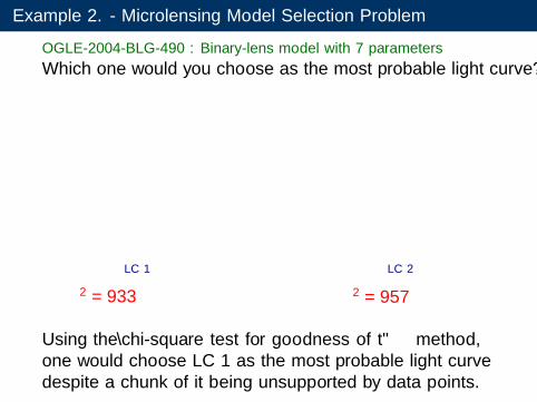
Example 2. - Microlensing Model Selection Problem
OGLE-2004-BLG-490 : Binary-lens model with 7 parameters
Which one would you choose as the most probable light curve?
LC 1 LC 2
χ2 = 933 χ2 = 957
Using the “chi-square test for goodness of fit” method,one would choose LC 1 as the most probable light curvedespite a chunk of it being unsupported by data points.
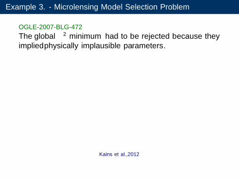
Example 3. - Microlensing Model Selection Problem
OGLE-2007-BLG-472
The global χ2 minimum had to be rejected because theyimplied physically implausible parameters.
Kains et al.,2012
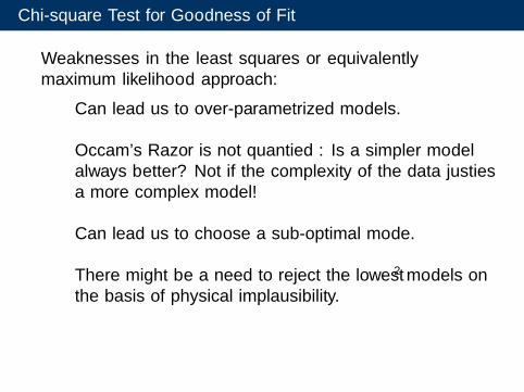
Chi-square Test for Goodness of Fit
Weaknesses in the least squares or equivalentlymaximum likelihood approach:
Can lead us to over-parametrized models.
Occam’s Razor is not quantified : Is a simpler modelalways better? Not if the complexity of the data justifiesa more complex model!
Can lead us to choose a sub-optimal mode.
There might be a need to reject the lowest χ2 models onthe basis of physical implausibility.
The Bayesian Approach to Model Selection
Model selection is a difficult task because wecan not simply choose the model that best fitsthe data.
The Bayesian approach offers a much morepowerful way of comparing models.

The Bayesian Evidence for Model Selection
Bayes’ Theorem:Posterior × Evidence = Likelihood × Prior (1)
Evidence:
Normalizes the posterior as a probability distribution overall the parameters.
Quantitative “evidence” in favour of one model overanother.
Naturally implements Occam’s razor and guards againstover-fitting.
Computationally expensive but crucial for model selectionproblems.

Bayesian Model Selection via Baye’s Factor
Given two models M1 and M2 we can decide which one isfavoured by simply computing Bayes’ Factor, the ratio of themodel evidences:
K =Z1
Z2(2)
A value of K > 1 means that M1 is more strongly supportedby the data under consideration than M2.

Nested Sampling - Model Selection & Parameter Estimation
Monte Carlo optimization method developed by JohnSkilling, 2004.
Performs straightforward model comparison bydirect computations of the Bayesian evidence.
Achieves simultaneous Bayesian model selection andBayesian parameter estimation as a by-product.

Nested Sampling
Image credit: Feroz et al., 2013
A population of points are randomly sampled. For iteration,i , the point with lowest likelihood value, Li , is removedfrom the live point set and replaced by another point drawnfrom the prior under the constraint that its likelihood ishigher than Li
MultiNest
Nested sampling based algorithm, introduced by Feroz,Hobson and Bridges.
Explores multi-modal and moderately multi-dimensionalparameter space successfully.
Active region nests inwards as the prior domain gets restrictedby the minimum likelihood condition.

PyMultiNest
The MultiNest sampling engine has a python interface -PyMultiNest, written by Johannes Buchner.
Two main input functions:
• Prior.
• Log-likelihood.

PyMultiNest
The MultiNest sampling engine has a python interface -PyMultiNest, written by Johannes Buchner.
Two main input functions:
• Prior.
• Log-likelihood.

PyMultiNest - Prior
Prior:Needs to transform the native parameter space uniformlydistributed in [0, 1] to physical parameters specific to theproblem.
Prior function

PyMultiNest - Prior
Prior:Needs to transform the native parameter space uniformlydistributed in [0, 1] to physical parameters specific to theproblem.
Prior function
PyMultiNest - Log-likelihood
Log-likelihood: constant - χ2
2
Log-likelihood function

PyMultiNest Outputs
Outputs:
• Maximum a posterior (MAP) parameters of all the modesfound.
• Local log-evidences of all the modes found and the globallog-evidence.
Straightforward model comparison by taking the ratio ofthe log-evidences.
Summary
GPU-accelerated code - fast and efficient parameterestimation.
Magnification Map Technique.• Grid-search with downhill simplex optimization method - for
rough initial models.
Dynamic Light Curve Engine.• Orbital motion modelling enabled.
• Mcmc optimization method - for more accurate models.
Nested Sampling Method for Model Selection.

Primary Research Goals
Solve the microlensing model selection problem using nestedsampling optimization.
Write code to enable MultiNest optimization with theDynamic Light Curve Engine.
Test and validate code by comparison with publishedmicrolensing results.
Model current microlensing events.

Primary Research Goals
Solve the microlensing model selection problem using nestedsampling optimization.
Write code to enable MultiNest optimization with theDynamic Light Curve Engine.
Test and validate code by comparison with publishedmicrolensing results.
Model current microlensing events.

Primary Research Goals
Solve the microlensing model selection problem using nestedsampling optimization.
Write code to enable MultiNest optimization with theDynamic Light Curve Engine.
Test and validate code by comparison with publishedmicrolensing results.
Model current microlensing events.

Primary Research Goals
Solve the microlensing model selection problem using nestedsampling optimization.
Write code to enable MultiNest optimization with theDynamic Light Curve Engine.
Test and validate code by comparison with publishedmicrolensing results.
Model current microlensing events.

Acknowledgements
Dr. Nicholas Rattenbury
Joe Ling.
Dr. Brendon Brewer