Embed Size (px)
Citation preview

大規模データから単語の 意味表現学習-word2vec
ボレガラ ダヌシカ 博士(情報理工学)
英国リバープール大学計算機科学科准教授
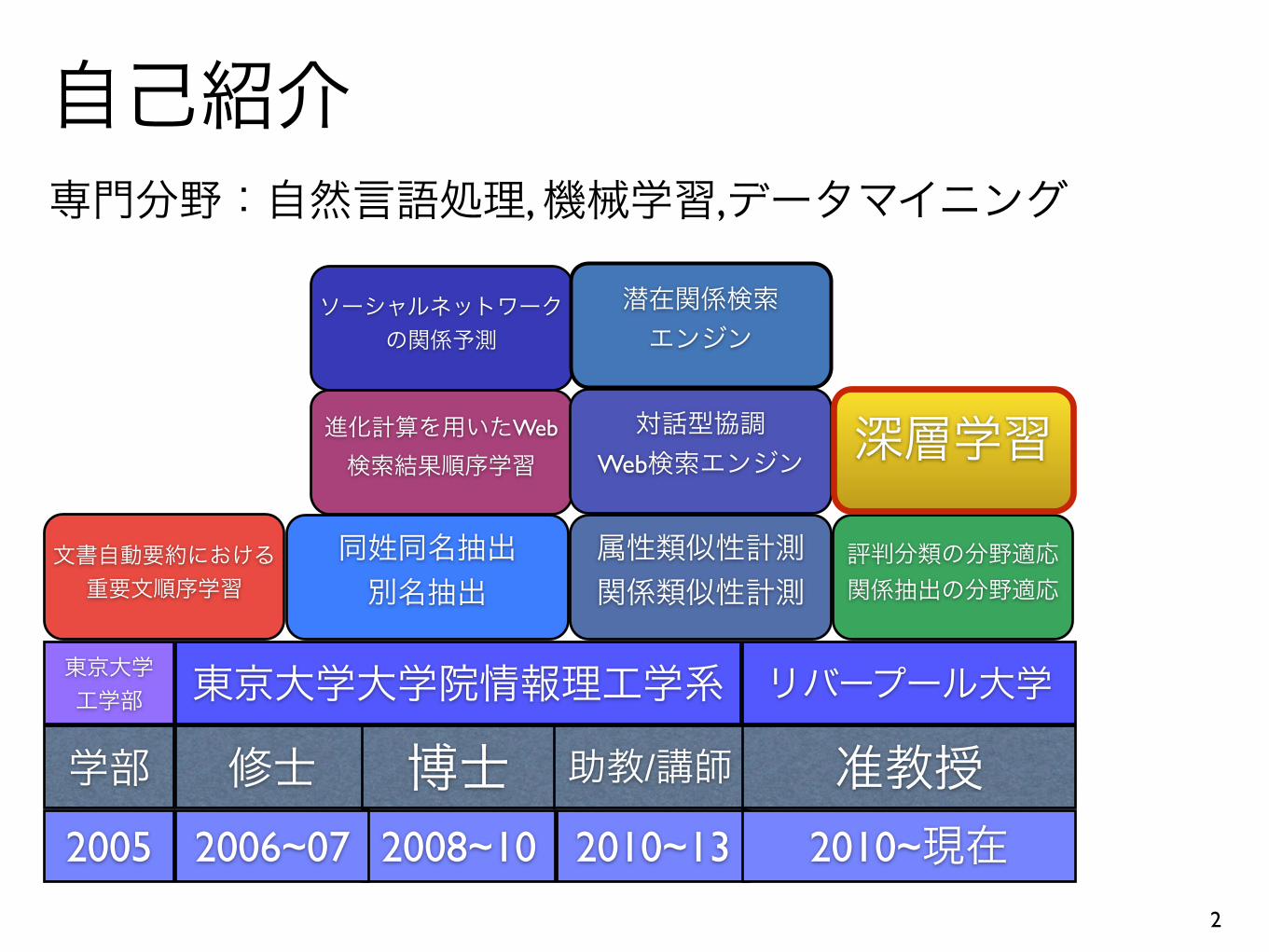
2
2005 2008~10
学部 修士 博士 助教/講師
東京大学 工学部 東京大学大学院情報理工学系
文書自動要約における重要文順序学習
同姓同名抽出 別名抽出
属性類似性計測 関係類似性計測
評判分類の分野適応 関係抽出の分野適応
進化計算を用いたWeb
検索結果順序学習
ソーシャルネットワークの関係予測
対話型協調 Web検索エンジン
潜在関係検索 エンジン
自己紹介専門分野:自然言語処理, 機械学習,データマイニング
2006~07 2010~13 2010~現在准教授
リバープール大学
深層学習

今回の講演の背景•深層学習に関する活動
• 2014年9月に深層学習のチュートリアルをCyberAgent社で行った.
•「深層学習」に関する書籍を分担執筆しており,今年の夏ごろ販売予定.
•研究活動
•意味的関係に関する意味表現学習
•国際会議AAAI’15(American Association for Artificial Intelligence)にて口頭発表.
•人工知能分野の最高峰の国際会議
3

単語の意味とは?
•語彙意味論(lexical semantics)
•数学的には語彙意味は「演算」である.
•自然言語の最小の意味単位は単語であり,単語の意味さえ表現しておけば,句(phrase),文(sentence),文書(document)の意味が構築できる.
•構成的意味論(compositional semantics)
4
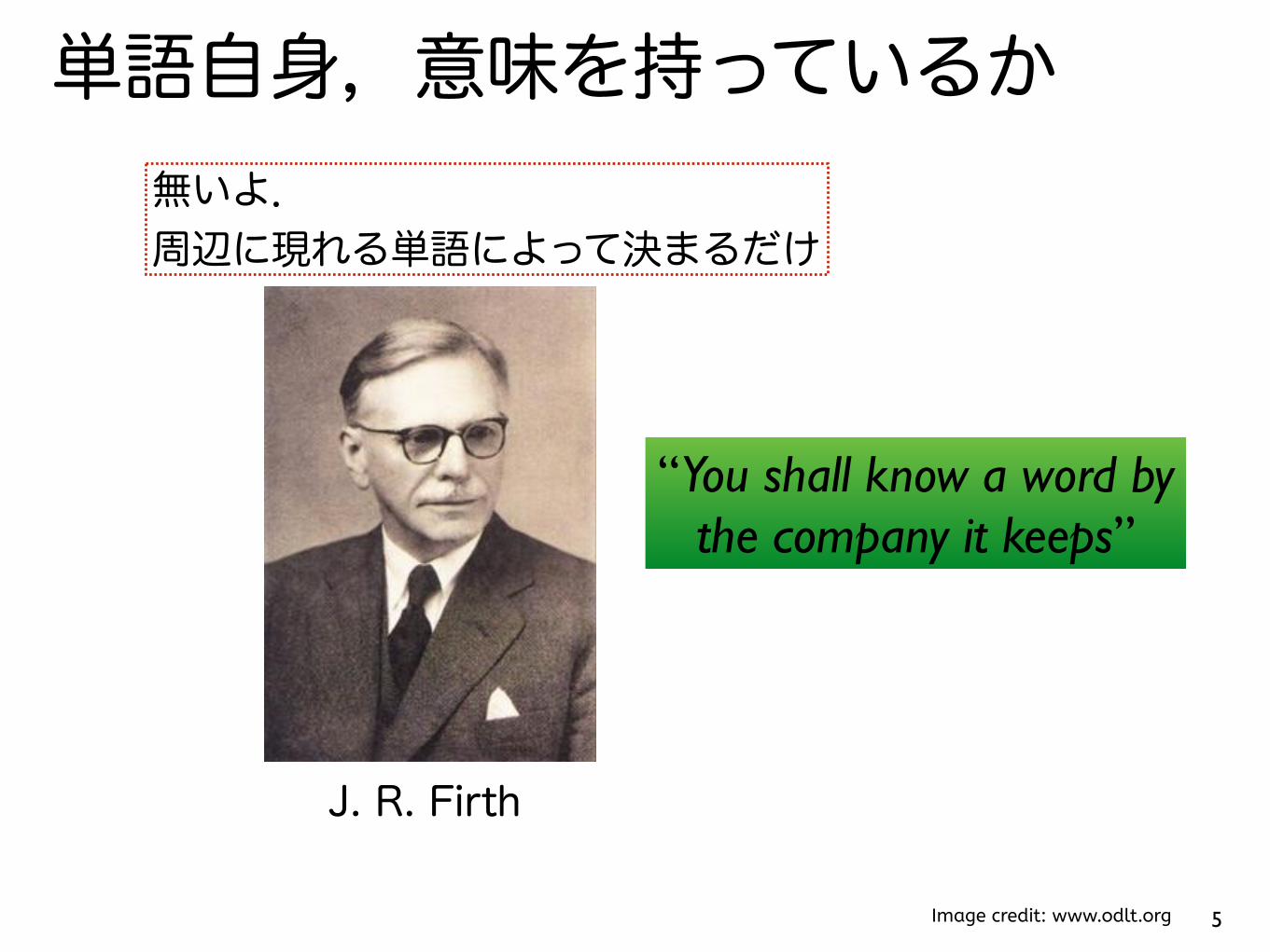
単語自身,意味を持っているか無いよ. 周辺に現れる単語によって決まるだけ
J. R. Firth
Image credit: www.odlt.org 5
“You shall know a word by the company it keeps”

問1
•X は持ち歩く可能で,相手と通信ができて,ネットも見れて,便利だ.X は次の内どれ?
•犬
•飛行機
• iPhone
•バナナ
6
でもそれは本当?•だって辞書は単語の意味を定義しているじゃないか
•辞書も他の単語との関係を述べることで単語の意味を説明している.
•膨大なコーパスがあれば周辺単語を集めてくるだけで単語の意味表現が作れるので自然言語処理屋には嬉しい.
• practicalな意味表現手法
•色んなタスクに応用して成功しているので意味表現として(定量的に)は正しい
7

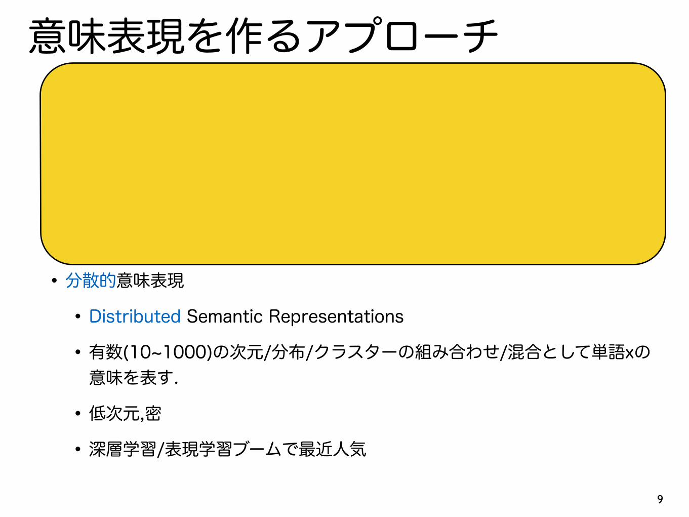
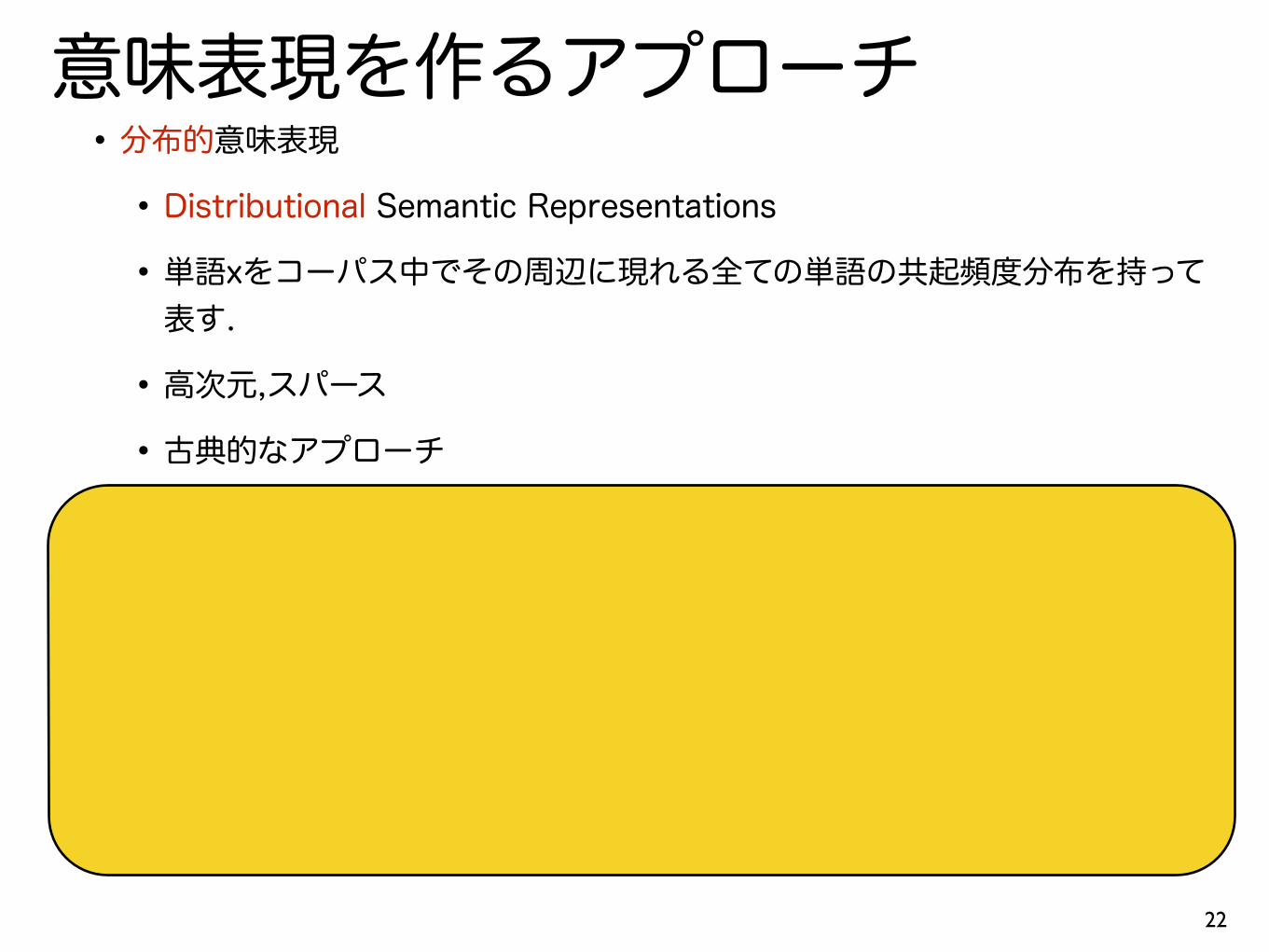
意味表現を作るアプローチ•分布的意味表現
•Distributional Semantic Representations
•単語xをコーパス中でその周辺に現れる全ての単語の共起頻度分布を持って表す.
•高次元,スパース
•古典的なアプローチ
•分散的意味表現
•Distributed Semantic Representations
•有数(10~1000)の次元/分布/クラスターの組み合わせ/混合として単語xの意味を表す.
•低次元,密
•深層学習/表現学習ブームで最近人気
8
意味表現を作るアプローチ•分布的意味表現
•Distributional Semantic Representations
•単語xをコーパス中でその周辺に現れる全ての単語の共起頻度分布を持って表す.
•高次元,スパース
•古典的なアプローチ
•分散的意味表現
•Distributed Semantic Representations
•有数(10~1000)の次元/分布/クラスターの組み合わせ/混合として単語xの意味を表す.
•低次元,密
•深層学習/表現学習ブームで最近人気
9

分布的意味表現構築
•「リンゴ」の単語の意味表現を作りなさい.
• S1=リンゴは赤い.
• S2=リンゴは美味しい.
• S3=青森県はリンゴの生産地として有名である.
10
分布的意味表現構築
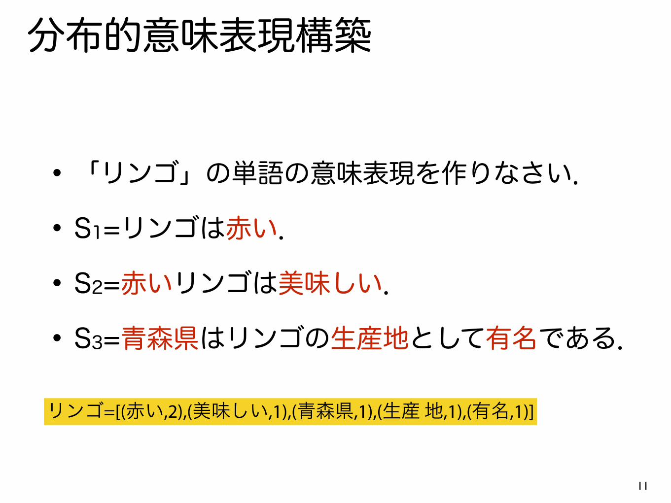
•「リンゴ」の単語の意味表現を作りなさい.
• S1=リンゴは赤い.
• S2=赤いリンゴは美味しい.
• S3=青森県はリンゴの生産地として有名である.
リンゴ=[(赤い,2),(美味しい,1),(青森県,1),(生産 地,1),(有名,1)]
11
応用例:意味的類似性計測
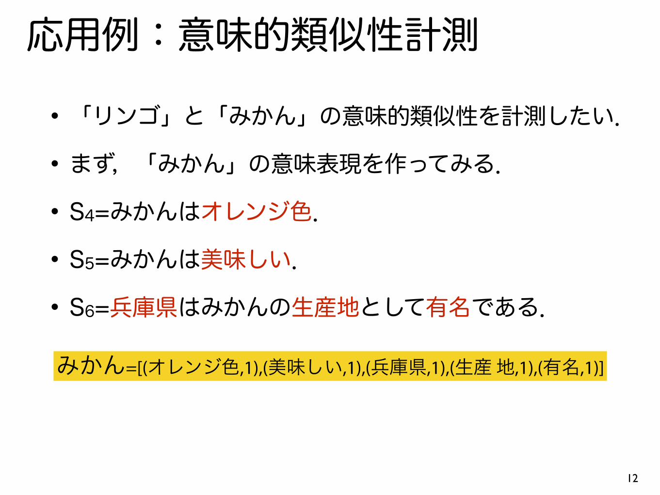
•「リンゴ」と「みかん」の意味的類似性を計測したい.
•まず,「みかん」の意味表現を作ってみる.
• S4=みかんはオレンジ色.
• S5=みかんは美味しい.
• S6=兵庫県はみかんの生産地として有名である.
12
みかん=[(オレンジ色,1),(美味しい,1),(兵庫県,1),(生産 地,1),(有名,1)]
「リンゴ」と「みかん」
13
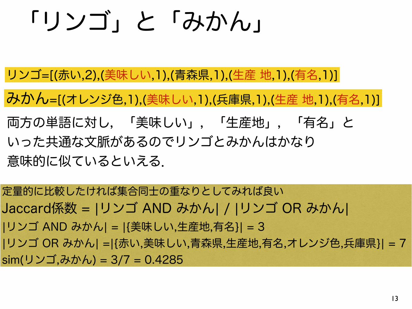
リンゴ=[(赤い,2),(美味しい,1),(青森県,1),(生産 地,1),(有名,1)]
みかん=[(オレンジ色,1),(美味しい,1),(兵庫県,1),(生産 地,1),(有名,1)]
両方の単語に対し,「美味しい」,「生産地」,「有名」と いった共通な文脈があるのでリンゴとみかんはかなり 意味的に似ているといえる.
定量的に比較したければ集合同士の重なりとしてみれば良い Jaccard係数 = |リンゴ AND みかん| / |リンゴ OR みかん| |リンゴ AND みかん| = |{美味しい,生産地,有名}| = 3 |リンゴ OR みかん| =|{赤い,美味しい,青森県,生産地,有名,オレンジ色,兵庫県}| = 7 sim(リンゴ,みかん) = 3/7 = 0.4285
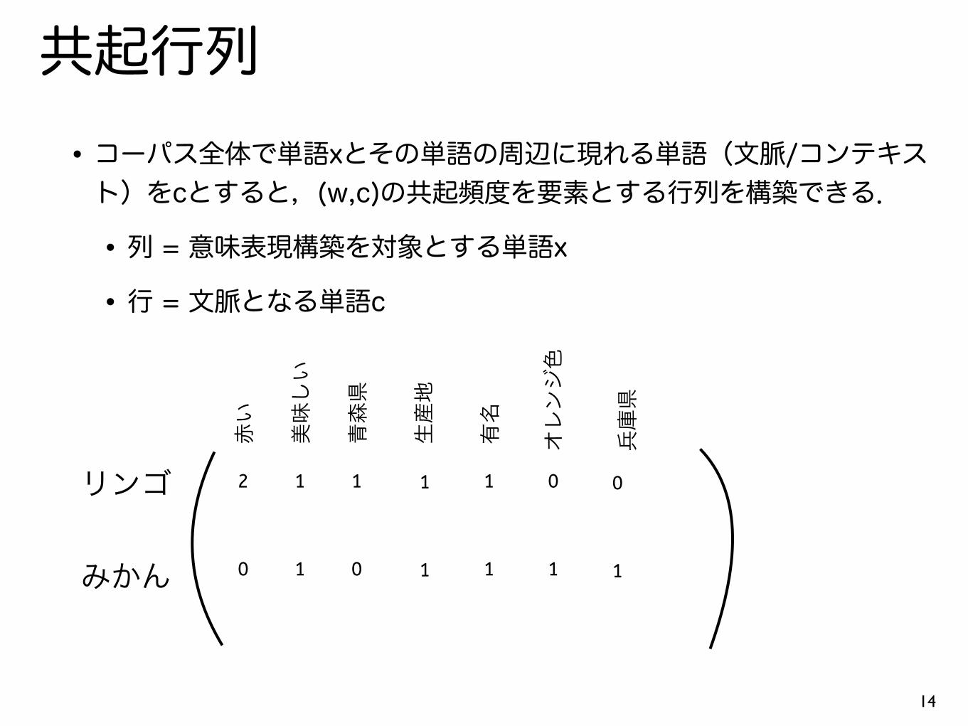
共起行列•コーパス全体で単語xとその単語の周辺に現れる単語(文脈/コンテキスト)をcとすると,(w,c)の共起頻度を要素とする行列を構築できる.
•列 = 意味表現構築を対象とする単語x
•行 = 文脈となる単語c
14
リンゴ
みかん
赤い
美味しい
青森県
生産地
有名
オレンジ色
兵庫県
2 1 1 1 1 0 0
0 1 0 1 1 1 1

大きな共起による問題
•ナマの共起頻度を信頼できるか.
•Googleヒット件数
• (car, automobile) = 11,300,000
• (car, apple) = 49,000,000
•では,carはautomobileよりappleに近いか?
•何らかの重み付けが必要
15

共起頻度の重み付け手法•沢山ありますが,それぞれの単語の出現頻度h(x), h(y)と単語同士の共起頻度h(x,y)の関数であることが殆ど
•重み = f(h(x), h(y), h(x,y))
•有名な重み付け手法
•点情報量(pointwise mutual information)
PMI(x, y) = log
✓p(x, y)
p(x)p(y)
◆= log
✓h(x, y)/N
(h(x)/N)⇥ (h(y)/N)
◆
16

その他の重み手法•正点情報量(PPMI) [Turney+Pantel JAIR’10]
• Positive pointwise mutual information
• PPMI(x,y) = max(0, PMI(x,y))
•移動点情報量(SPMI) [Levy+Goldberg NIPS’14]
• Shifted pointwise mutual information
• SPMI(x,y) = PMI(x,y) - log(k)
• kは定数
17
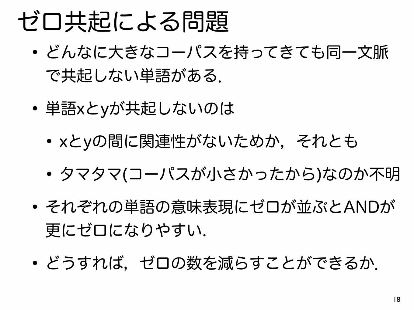
ゼロ共起による問題•どんなに大きなコーパスを持ってきても同一文脈で共起しない単語がある.
•単語xとyが共起しないのは
• xとyの間に関連性がないためか,それとも
•タマタマ(コーパスが小さかったから)なのか不明
•それぞれの単語の意味表現にゼロが並ぶとANDが更にゼロになりやすい.
•どうすれば,ゼロの数を減らすことができるか.
18

次元削減/低次元射影•結局何らかの空間で意味を表せばよい.作った意味表現を使って正確に類似度計測できれば良い.
•文脈の次元を減らすことでゼロとなっていたものをゼロでない値で埋める.
19
リンゴ
みかん
赤い 美味しい
青森県
生産地
有名
オレンジ色
兵庫県
2 1 1 1 1 0 0
0 1 0 1 1 1 1
リンゴ
みかん
次元
1
0.3 0.2 1
1.2 -0.1 0.3
次元
2
次元
3
行の数が変わらないので元々あった単語が全てに対して
意味表現が構築される.列の数が減る(次元削減)
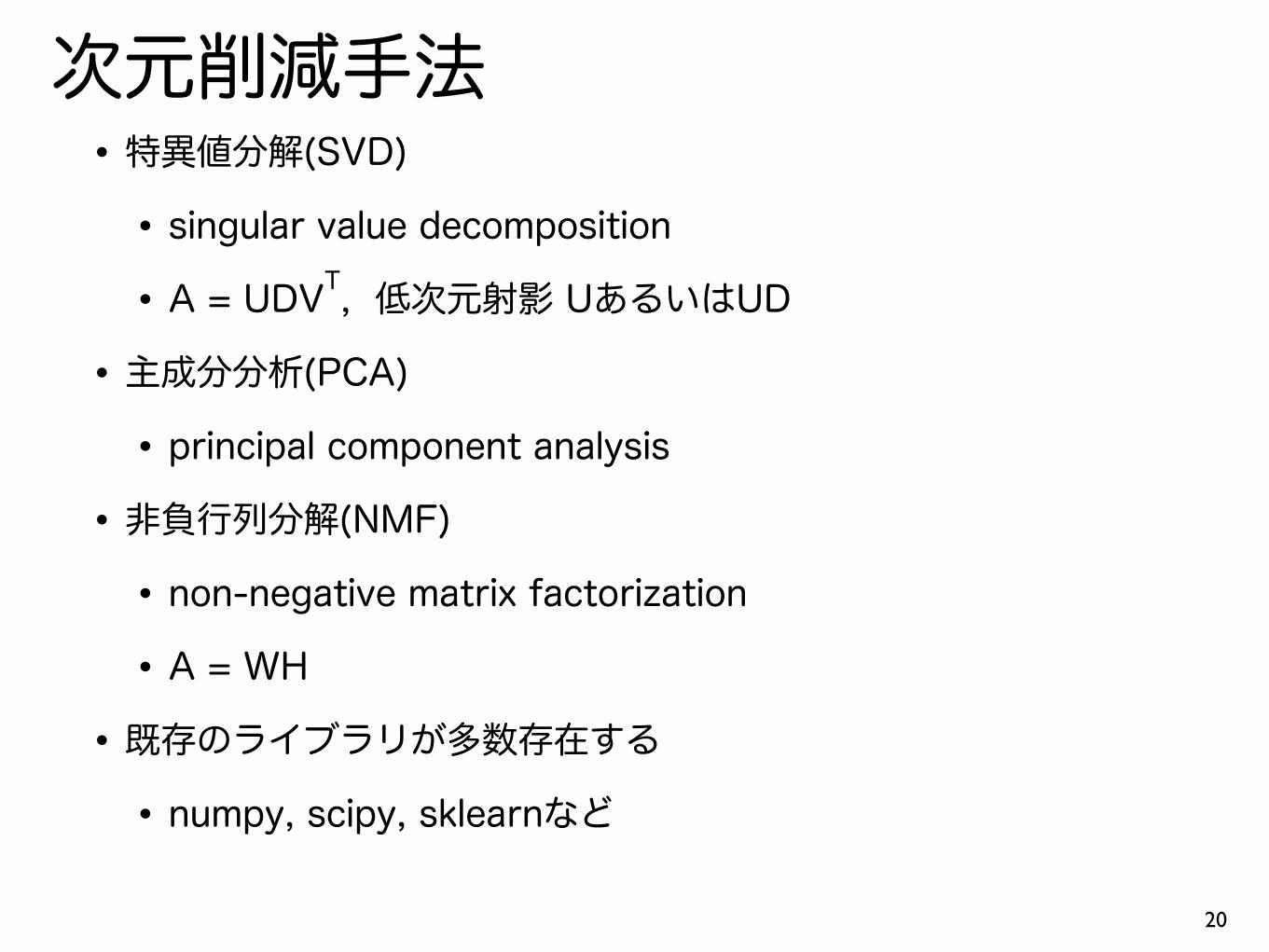
次元削減手法•特異値分解(SVD)
• singular value decomposition
• A = UDVT, 低次元射影 UあるいはUD
•主成分分析(PCA)
• principal component analysis
•非負行列分解(NMF)
• non-negative matrix factorization
• A = WH
•既存のライブラリが多数存在する
• numpy, scipy, sklearnなど
20

細かい工夫が多数•文脈として何を選ぶか
•文全体 (sentence-level co-occurrences)
•前後のn単語 (proximity window)
•係り受け関係にある単語 (dependencies)
•文脈の距離によって重みをつける.
•遠ければその共起の重みを距離分だけ減らす
•などなど
21
意味表現を作るアプローチ•分布的意味表現
•Distributional Semantic Representations
•単語xをコーパス中でその周辺に現れる全ての単語の共起頻度分布を持って表す.
•高次元,スパース
•古典的なアプローチ
•分散的意味表現
•Distributed Semantic Representations
•有数(10~1000)の次元/分布/クラスターの組み合わせ/混合として単語xの意味を表す.
•低次元,密
•深層学習/表現学習ブームで最近人気
22
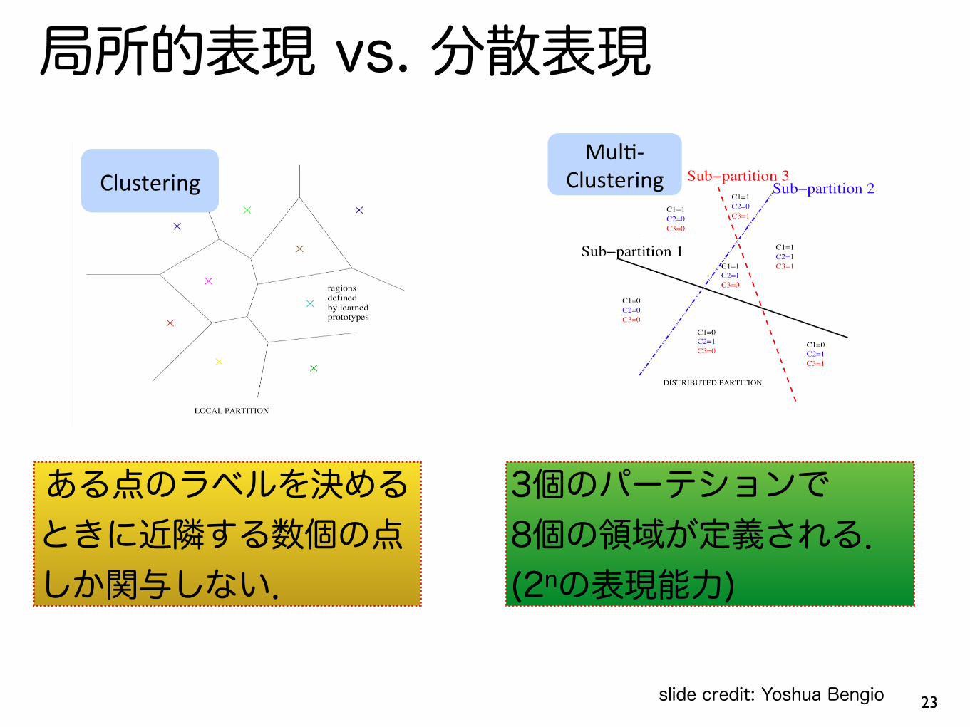
局所的表現 vs. 分散表現
23
• Clustering,!NearestJNeighbors,!RBF!SVMs,!local!nonJparametric!density!es>ma>on!&!predic>on,!decision!trees,!etc.!
• Parameters!for!each!dis>nguishable!region!
• #!dis>nguishable!regions!linear!in!#!parameters!
#2 The need for distributed representations Clustering!
16!
• Factor!models,!PCA,!RBMs,!Neural!Nets,!Sparse!Coding,!Deep!Learning,!etc.!
• Each!parameter!influences!many!regions,!not!just!local!neighbors!
• #!dis>nguishable!regions!grows!almost!exponen>ally!with!#!parameters!
• GENERALIZE+NON5LOCALLY+TO+NEVER5SEEN+REGIONS+
#2 The need for distributed representations
Mul>J!
Clustering!
17!
C1! C2! C3!
input!
ある点のラベルを決める ときに近隣する数個の点 しか関与しない.
3個のパーテションで 8個の領域が定義される. (2nの表現能力)
slide credit: Yoshua Bengio

分散表現の表現能力
24
美味しさ 赤さ 青森県らしさ
有名度
兵庫県 らしさ
オレンジ色度

分散表現の表現能力
25
美味しさ 赤さ 青森県らしさ
有名度
兵庫県 らしさ
オレンジ色度
リンゴ

分散表現の表現能力
26
美味しさ 赤さ 青森県らしさ
有名度
兵庫県 らしさ
オレンジ色度
みかん

分散表現を学習する•分布表現はコーパスから数え上げた
• counting-based approach
•ボトムアップ型
•一方,分散表現ではまず,各単語xの意味表現がd次元のベクトルで表させると仮定し,そのベクトルの要素の値をコーパスから学習する.
• prediction-based approach
• xの意味表現ベクトルv(x)を使って,コーパス中でxの周辺に出現する単語cを予測できるかどうかで学習する.
•トップダウン型
•次数dを固定.最初にランダムベクトルで初期化する.
27

word2vec
•word2vecは単語の分散意味表現を学習するためのツールであり,次の2つの手法が実装されている.
• skip-gram(スキップグラム)モデル
• continuous bag-of-words(CBOW)(連続単語集合)モデル
28
n-gram vs. skip-gram
•連続する単語列のことをn-gram(n-グラム)と呼ばれている.
•例:I went to school
• bi-gram = I+went, went+to, to+school
•スキップグラムでは連続していなくてもOK
• skip bi-gramの例: I+to, went+school
29

skip-gramモデル
30
私はみそ汁とご飯を頂いた
skip-gramモデル
31
私はみそ汁とご飯を頂いた
私 は みそ汁 と ご飯 を 頂いた形態素解析
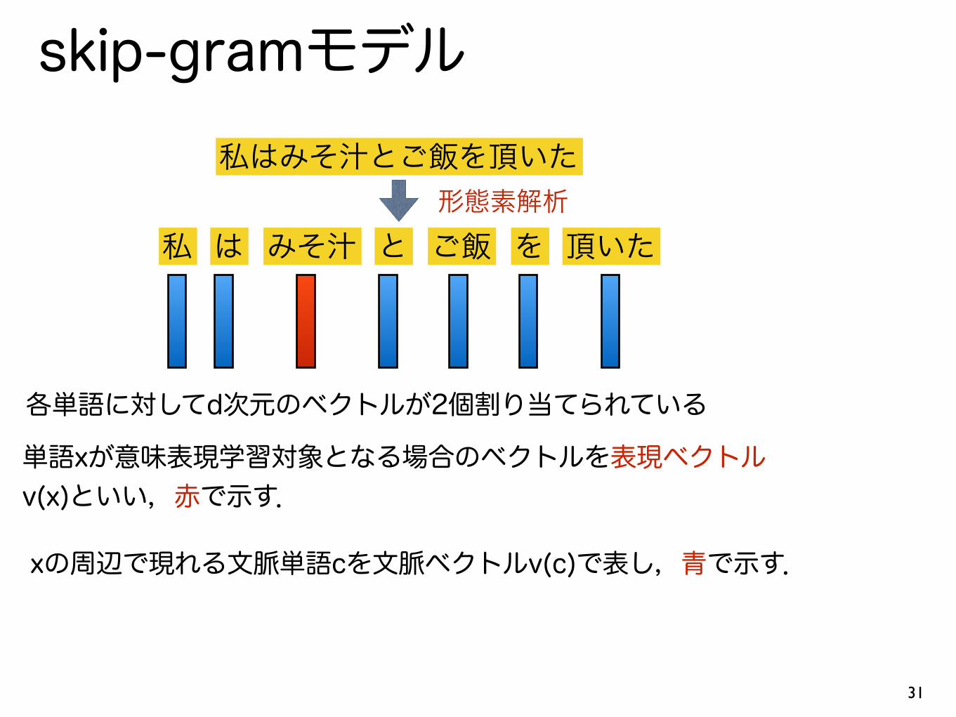
各単語に対してd次元のベクトルが2個割り当てられている
単語xが意味表現学習対象となる場合のベクトルを表現ベクトル v(x)といい,赤で示す.
xの周辺で現れる文脈単語cを文脈ベクトルv(c)で表し,青で示す.

skip-gramモデル
32
私はみそ汁とご飯を頂いた
私 は みそ汁 と ご飯 を 頂いた形態素解析
v(x) u(c)
例えば「みそ汁」の周辺で「ご飯」が出現するかどうか を予測する問題を考えよう.
skip-gramモデル
33
私はみそ汁とご飯を頂いた
私 は みそ汁 と ? を 頂いた形態素解析
v(x) u(c)
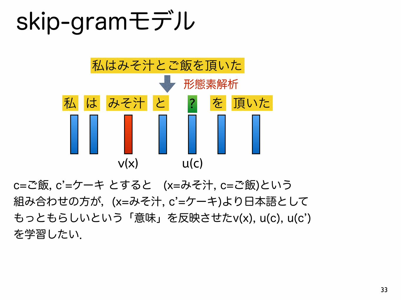
c=ご飯, c’=ケーキ とすると (x=みそ汁, c=ご飯)という 組み合わせの方が,(x=みそ汁, c’=ケーキ)より日本語として もっともらしいという「意味」を反映させたv(x), u(c), u(c’) を学習したい.

skip-gramモデル
34
私はみそ汁とご飯を頂いた
私 は みそ汁 と ? を 頂いた形態素解析
v(x) v(c)
提案1 この尤もらしさをベクトルの内積で定義しましょう. score(x,c) = v(x)Tu(c)
skip-gramモデル
35
私はみそ汁とご飯を頂いた
私 は みそ汁 と ? を 頂いた形態素解析
v(x) u(c)
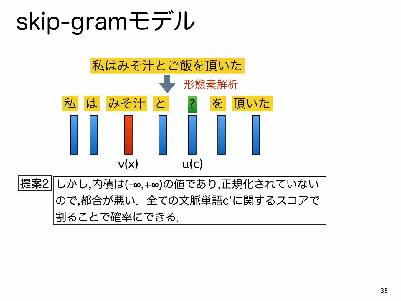
提案2 しかし,内積は(-∞,+∞)の値であり,正規化されていない ので,都合が悪い.全ての文脈単語c’に関するスコアで 割ることで確率にできる.

対数双線型• log-bilinear model
36
xの周辺でcが 出現する確率
xとcの共起しやすさ
語彙集合(V)に含まれる全ての単語 c’とxが共起しやすさ
[Mnih+Hinton ICML’07]
p(c|x) = exp(v(x)>u(c))Pc02V exp(v(x)>u(c0))
学習方法は
ロジスティック回帰と
似ている.vとuの
どちらか片方を固定すれば
もう片方に関し,
ロジスティック回帰を
解いているのと同様.
one-vs-restの学習.
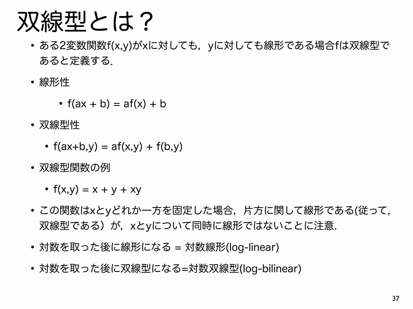
双線型とは?•ある2変数関数f(x,y)がxに対しても,yに対しても線形である場合fは双線型であると定義する.
•線形性
• f(ax + b) = af(x) + b
•双線型性
• f(ax+b,y) = af(x,y) + f(b,y)
•双線型関数の例
• f(x,y) = x + y + xy
•この関数はxとyどれか一方を固定した場合,片方に関して線形である(従って,双線型である)が,xとyについて同時に線形ではないことに注意.
•対数を取った後に線形になる = 対数線形(log-linear)
•対数を取った後に双線型になる=対数双線型(log-bilinear)
37
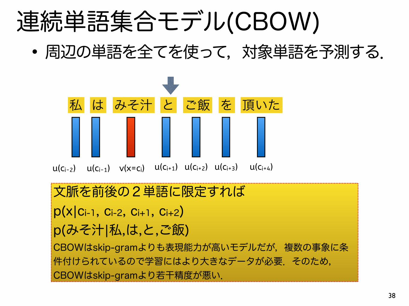
連続単語集合モデル(CBOW)•周辺の単語を全てを使って,対象単語を予測する.
38
私 は みそ汁 と ご飯 を 頂いた
u(ci+1) u(ci+2) u(ci+3) u(ci+4)u(ci-1)u(ci-2) v(x=ci)
文脈を前後の2単語に限定すれば p(x|ci-1, ci-2, ci+1, ci+2) p(みそ汁|私,は,と,ご飯) CBOWはskip-gramよりも表現能力が高いモデルだが,複数の事象に条件付けられているので学習にはより大きなデータが必要.そのため,CBOWはskip-gramより若干精度が悪い.

工夫
• log-bilinearモデルの分母の計算が重たい
•全語彙集合上でのexpの和を計算を要する
•工夫その1
•負例サンプリング(negative sampling)
•工夫その2
•階層的ソフトマックス(hierarchical softmax)
39

負例サンプリング
40
ロジスティック回帰の積ソフトマックス
正例 サンプリングした負例
Noise contrastive estimation [Mnih+Hinton ICML’12]
どうやってサンプリングするかp(unigram)0.75
c
p(c)0.75
コーパス中のそれぞれの単語をラベル として多値分類器を学習するのと等価
p(c|x) = exp(v(x)>u(c))Pc
02V exp(v(x)>u(c0))⇡ �(v(x)>u(c))
Y
c
02S(x)
�(�v(x)>u(c0))
単語(unigram)

階層的ソフトマックス•単語の出現の代わりに意味クラスの出現を使うことで語彙の大きさを減らす.
•全単語を階層構造(木)に当てはめ,ある単語の予測確率を根から単語(葉)に至るパス上の分岐点に対する確率(ロジスティック回帰でモデル化)の積として計算する.
41
根
具体物 抽象物
生物 無生物
動物 植物
犬 猫
1 0
1
1
1
0
0
0
p(猫)=p(根)p(具体物|根)p(生物|具体物)p(動物|生物)p(猫|動物)
Path(猫)={(根,1), (具体物,1), (生物,1), (動物,1)}
どのように木構造を作るか? クラスタリング,既存の語彙体系, ハフマン木
p(c|x) = exp(v(x)>u(c))Pc02V exp(v(x)>u(c0))
⇡Y
(yi,zi)2Path(c)0
�(ziv(x)>u(yi))

学習した意味表現の評価•学習した意味表現はベクトルであり「目で見て分かる」ものではない.
•正解が存在しない.(no gold standard)
•何らかのタスクに応用し,その性能向上度合いで評価をしなければならない
•間接的評価(extrinsic evaluation)
•単語間の意味的類似性計測
•アナロジー問題を解く42
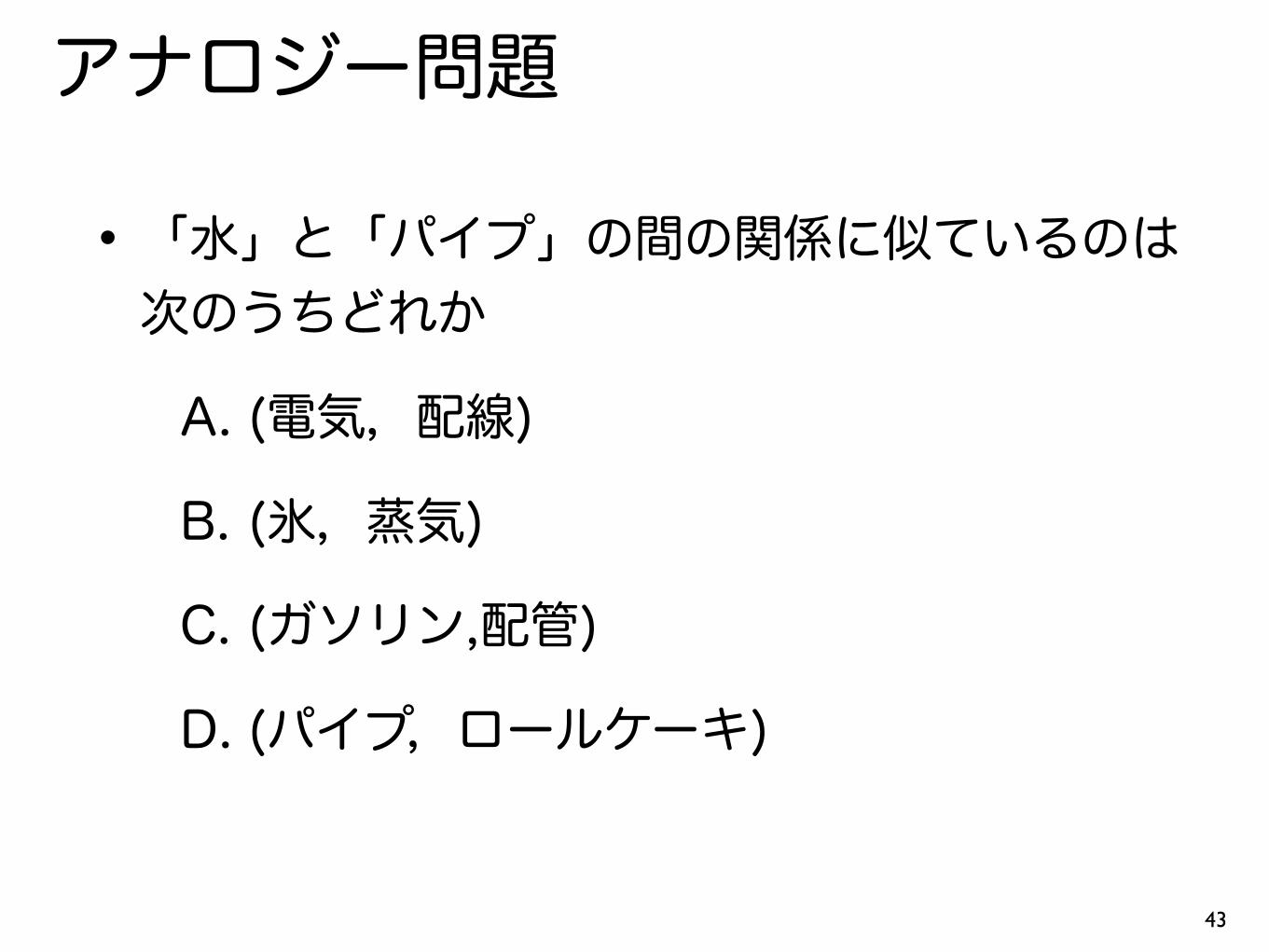
アナロジー問題
•「水」と「パイプ」の間の関係に似ているのは次のうちどれか
A. (電気,配線)
B. (氷,蒸気)
C. (ガソリン,配管)
D. (パイプ,ロールケーキ)
43

意味的類似性による評価•与えられた単語対に対し,人間(言語学者,Turker)がその2つの単語がどれくらい似ているかスコア付けを行い,平均を求める.
•人間が付けたスコアとアルゴリズムが出したスコア間の相関係数(Pearson/Spearman順序相関)を計測する.
•人間との相関が高い類似度スコアを出力するアルゴリズムの方が良い.
44

アナロジーを解く
•(man, king)ならば(woman, ?)
•手順
• x = v(king) - v(man) + v(woman)を作る.
•このxと語彙中の全ての単語とのコサイン類似度を計測し,最大な類似度を持つ単語を答えとして返す.
45

Global Vector Prediction (GloVe)•skip-gramとCBOWは一文単位でコーパスを処理し,意味表現学習していく.
•オンライン学習
•大規模なコーパスからでも容易に(処理時間が文数と線形に増加,分割による並列化可能)できる.
•一方,分布表現ではコーパス全体から共起行列を作っている.
•コーパス全体の共起情報を使って意味表現学習ができないか.
• Pennington+ EMNLP’14, Global Vectors for Word Representation
46
予測誤差 バイアス項 共起頻度
内積と共起の対数間の自乗誤差を最小化している. 理由:ベクトルの引き算で意味を特徴付けたい. ポイント:log(a/b) = log(a) - log(b)
J =
|V|X
i,j
f(Mi,j)�v(xi)
>v(xj) + bi + bj � logMi,j
�2
頻度による重み
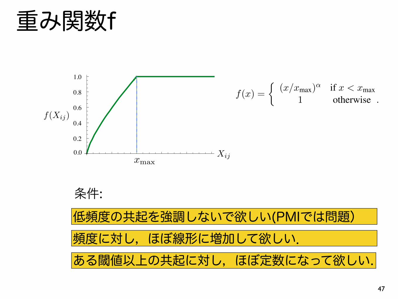
重み関数f
47
Next, we note that Eqn. (6) would exhibit the ex-change symmetry if not for the log(X
i
) on theright-hand side. However, this term is indepen-dent of k so it can be absorbed into a bias b
i
forwi
. Finally, adding an additional bias ˜bk
for w̃k
restores the symmetry,
wT
i
w̃k
+ bi
+
˜bk
= log(Xik
) . (7)
Eqn. (7) is a drastic simplification over Eqn. (1),but it is actually ill-defined since the logarithm di-verges whenever its argument is zero. One resolu-tion to this issue is to include an additive shift inthe logarithm, log(X
ik
) ! log(1 + Xik
), whichmaintains the sparsity of X while avoiding the di-vergences. The idea of factorizing the log of theco-occurrence matrix is closely related to LSA andwe will use the resulting model as a baseline in ourexperiments. The main problem with this modelis that it weights all co-occurrences equally, eventhose that happen rarely or never. Such rare co-occurrences are noisy and do not carry as muchinformation as the more frequent ones — yet evenjust the zero entries account for 75–95% of thedata in X , depending on the vocabulary size andcorpus.
We propose a new weighted least squares re-gression model that addresses these problems.Casting Eqn. (7) as a least squares problem, andintroducing a weighting function f(X
ij
) into thecost function gives us the model,
J =
VX
i,j=1
f (Xij
)
⇣wT
i
w̃j
+ bi
+
˜bj
� logXij
⌘2,
(8)where V is the size of the vocabulary. The weight-ing function should obey the following properties:
1. f(0) = 0. If f is viewed as a continuousfunction, it should vanish as x ! 0 fastenough that the lim
x!0 f(x) log2 x is finite.
2. f(x) should be non-decreasing so that rareco-occurrences are not overweighted.
3. f(x) should be relatively small for large val-ues of x, so that frequent co-occurrences arenot overweighted.
Of course a large number of functions satisfy theseproperties, but one class of functions that we foundto work well can be parameterized as,
f(x) =
⇢(x/xmax)
↵ if x < xmax1 otherwise .
(9)
0.2
0.4
0.6
0.8
1.0
0.0
Figure 1: Weighting function f with ↵ = 3/4.
The performance of the model depends weakly onthe cutoff, which we fix to xmax = 100 for all ourexperiments. We found that ↵ = 3/4 gives a mod-est improvement over a linear version with ↵ = 1.Although we offer only empirical motivation forchoosing the value 3/4, it is interesting that a sim-ilar fractional power scaling was found to give thebest performance in (Mikolov et al., 2013a).
3.1 Relationship to Other Models
Because all unsupervised methods for learningword vectors are ultimately based on the occur-rence statistics of a corpus, there should be com-monalities between the models. Nevertheless, cer-tain models remain somewhat opaque in this re-gard, particularly the recent window-based meth-ods like skip-gram and ivLBL. Therefore, in thissubsection we will show how these models are re-lated to our proposed model, as defined in Eq. (8).
The starting point for the skip-gram or ivLBLmethods is a model Q
ij
for the probability thatword j appears in the context of word i. For con-creteness, let us assume that Q
ij
is a softmax,
Qij
=
exp(wT
i
w̃j
)
PV
k=1 exp(wT
i
w̃k
)
. (10)
Most of the details of these models are irrelevantfor our purposes, aside from the the fact that theyattempt to maximize the log probability as a con-text window scans over the corpus. Training pro-ceeds in an on-line, stochastic fashion, but the im-plied global objective function can be written as,
J = �X
i2corpusj2context(i)
logQij
. (11)
Evaluating the normalization factor of the soft-max for each term in this sum is costly. To al-low for efficient training, the skip-gram and ivLBLmodels introduce approximations to Q
ij
. How-ever, the sum in Eqn. (11) can be evaluated much
低頻度の共起を強調しないで欲しい(PMIでは問題) 頻度に対し,ほぼ線形に増加して欲しい. ある閾値以上の共起に対し,ほぼ定数になって欲しい.
条件:
Next, we note that Eqn. (6) would exhibit the ex-change symmetry if not for the log(X
i
) on theright-hand side. However, this term is indepen-dent of k so it can be absorbed into a bias b
i
forwi
. Finally, adding an additional bias ˜bk
for w̃k
restores the symmetry,
wT
i
w̃k
+ bi
+
˜bk
= log(Xik
) . (7)
Eqn. (7) is a drastic simplification over Eqn. (1),but it is actually ill-defined since the logarithm di-verges whenever its argument is zero. One resolu-tion to this issue is to include an additive shift inthe logarithm, log(X
ik
) ! log(1 + Xik
), whichmaintains the sparsity of X while avoiding the di-vergences. The idea of factorizing the log of theco-occurrence matrix is closely related to LSA andwe will use the resulting model as a baseline in ourexperiments. The main problem with this modelis that it weights all co-occurrences equally, eventhose that happen rarely or never. Such rare co-occurrences are noisy and do not carry as muchinformation as the more frequent ones — yet evenjust the zero entries account for 75–95% of thedata in X , depending on the vocabulary size andcorpus.
We propose a new weighted least squares re-gression model that addresses these problems.Casting Eqn. (7) as a least squares problem, andintroducing a weighting function f(X
ij
) into thecost function gives us the model,
J =
VX
i,j=1
f (Xij
)
⇣wT
i
w̃j
+ bi
+
˜bj
� logXij
⌘2,
(8)where V is the size of the vocabulary. The weight-ing function should obey the following properties:
1. f(0) = 0. If f is viewed as a continuousfunction, it should vanish as x ! 0 fastenough that the lim
x!0 f(x) log2 x is finite.
2. f(x) should be non-decreasing so that rareco-occurrences are not overweighted.
3. f(x) should be relatively small for large val-ues of x, so that frequent co-occurrences arenot overweighted.
Of course a large number of functions satisfy theseproperties, but one class of functions that we foundto work well can be parameterized as,
f(x) =
⇢(x/xmax)
↵ if x < xmax1 otherwise .
(9)
0.2
0.4
0.6
0.8
1.0
0.0
Figure 1: Weighting function f with ↵ = 3/4.
The performance of the model depends weakly onthe cutoff, which we fix to xmax = 100 for all ourexperiments. We found that ↵ = 3/4 gives a mod-est improvement over a linear version with ↵ = 1.Although we offer only empirical motivation forchoosing the value 3/4, it is interesting that a sim-ilar fractional power scaling was found to give thebest performance in (Mikolov et al., 2013a).
3.1 Relationship to Other Models
Because all unsupervised methods for learningword vectors are ultimately based on the occur-rence statistics of a corpus, there should be com-monalities between the models. Nevertheless, cer-tain models remain somewhat opaque in this re-gard, particularly the recent window-based meth-ods like skip-gram and ivLBL. Therefore, in thissubsection we will show how these models are re-lated to our proposed model, as defined in Eq. (8).
The starting point for the skip-gram or ivLBLmethods is a model Q
ij
for the probability thatword j appears in the context of word i. For con-creteness, let us assume that Q
ij
is a softmax,
Qij
=
exp(wT
i
w̃j
)
PV
k=1 exp(wT
i
w̃k
)
. (10)
Most of the details of these models are irrelevantfor our purposes, aside from the the fact that theyattempt to maximize the log probability as a con-text window scans over the corpus. Training pro-ceeds in an on-line, stochastic fashion, but the im-plied global objective function can be written as,
J = �X
i2corpusj2context(i)
logQij
. (11)
Evaluating the normalization factor of the soft-max for each term in this sum is costly. To al-low for efficient training, the skip-gram and ivLBLmodels introduce approximations to Q
ij
. How-ever, the sum in Eqn. (11) can be evaluated much

行列分解との等価性 [Levy+Goldberg NIPS14]
• (i,j)番目の要素をPMI(wi,cj) - log(k)とする行列Mを構築し, SVDによってMを分解することで単語の意味表現(U)とコンテキストの意味表現(V)を得ることができる.
• kはskip-gramで正例:負例の個数の割合
48
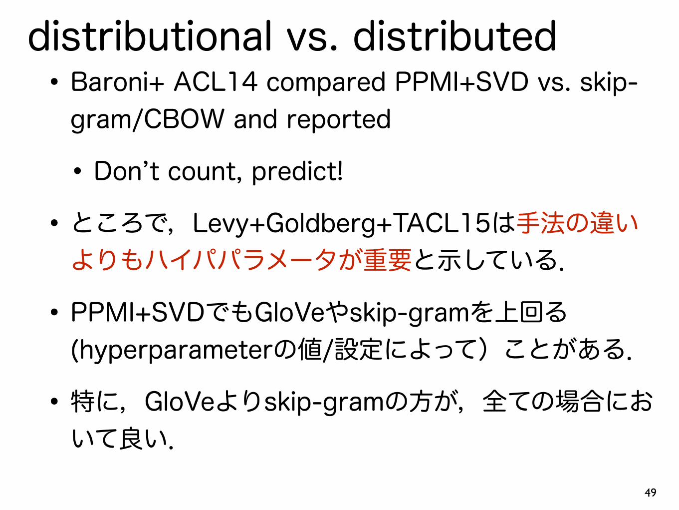
distributional vs. distributed•Baroni+ ACL14 compared PPMI+SVD vs. skip-gram/CBOW and reported
• Don’t count, predict!
•ところで,Levy+Goldberg+TACL15は手法の違いよりもハイパパラメータが重要と示している.
• PPMI+SVDでもGloVeやskip-gramを上回る(hyperparameterの値/設定によって)ことがある.
•特に,GloVeよりskip-gramの方が,全ての場合において良い.
49

PPMI+SVDの問題点
•「正」の共起しか見ていない.
• PPMIを計算するときに実際にxとcが共起しているという情報を使うがxとc’が共起していないという情報を使っていない.
• skip-gramは負例サンプリングでこの情報を把握している.
•GloVeもこの「負」の共起を使っていない.
50

ツール及び学習済み表現の紹介•Wikipedia,ウェブページ,新聞記事など様々なコーパスから学習された意味表現ベクトルが多数公開されている.
• GloVe [http://nlp.stanford.edu/projects/glove]
• word2vec [https://code.google.com/p/word2vec/]
• その他多数 [http://metaoptimize.com/projects/wordreprs]
• 自分のデータでGloVeとword2vecを学習し直すことも可能.
• ソース(C)を上述のリンクからダウンロード可能.
• 意味表現を学習する・ロードするためのPythonによるツール
• gensim [https://radimrehurek.com/gensim/models/word2vec.html]
51
意味表現の応用•単語レベルの応用
•関連語抽出,クエリ推奨,クエリ拡張
•文書レベルの応用
•広告とアドワードのマッチング
•評判分析
•その他
•関係の分類
•機械翻訳
•分野適応
52