ICDE2014 Session 14 Data Warehousing

Session 14: Data Warehousing

担当：若森拓馬（NTT）

【ICDE2014勉強会】

紹介する論文

2

1.  Distributed Interactive Cube Exploration N. Kamat, P. Jayachandran, K. Tunga, A. Nandi (Ohio State University)

2.  A Tunable Compression Framework for Bitmap Indices G. Guzun, G. Canahuate (The University of Iowa), D. Chiu (Washington State University), J. Sawin (University of St. Thomas)

3.  Pagrol: Parallel Graph OLAP over Large-scale Attributed Graphs Z. Wang, Q. Fan, H. Wang, K-L Tan (National University of Singapore), D. Agrawal, A. E. Abbadi (University of California)

Session 14: Data Warehousing 担当：若森拓馬（NTT）

Distributed Interactive Cube Exploration

3

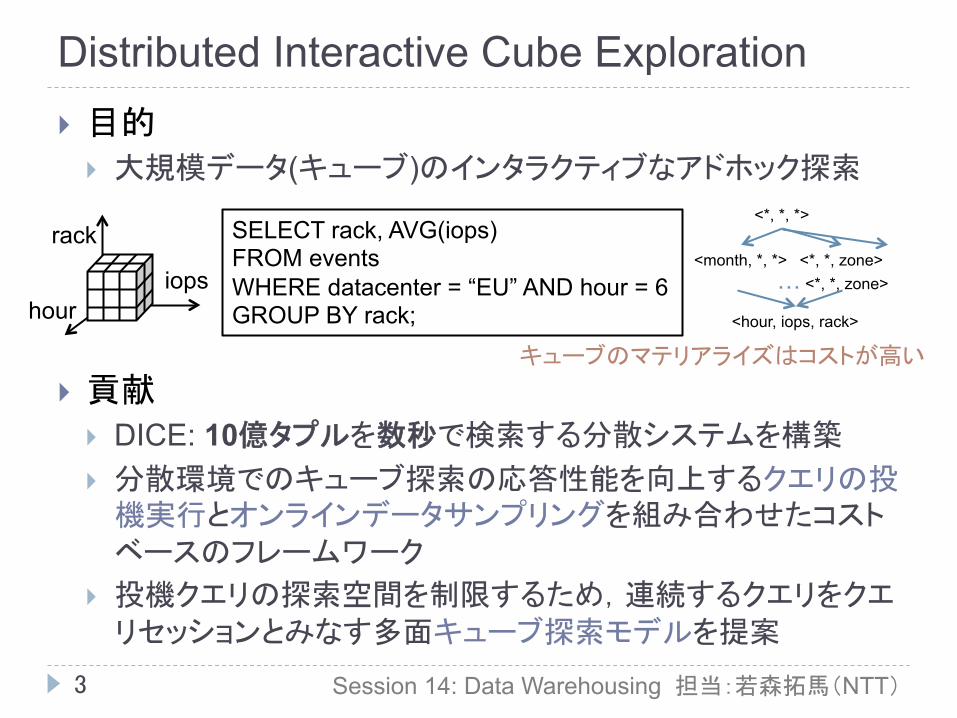
}  目的 }  大規模データ(キューブ)のインタラクティブなアドホック探索

}  貢献 }  DICE: 10億タプルを数秒で検索する分散システムを構築 }  分散環境でのキューブ探索の応答性能を向上するクエリの投

機実行とオンラインデータサンプリングを組み合わせたコストベースのフレームワーク

}  投機クエリの探索空間を制限するため，連続するクエリをクエリセッションとみなす多面キューブ探索モデルを提案


SELECT rack, AVG(iops) FROM events WHERE datacenter = “EU” AND hour = 6 GROUP BY rack;

rack

hour iops

<hour, iops, rack>

<*, *, *>

<month, *, *> <*, *, zone>

…

キューブのマテリアライズはコストが高い

<*, *, zone>


4

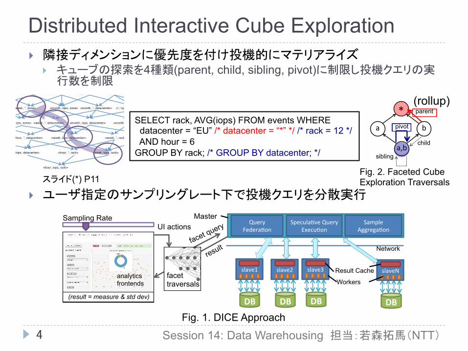
}  隣接ディメンションに優先度を付け投機的にマテリアライズ }  キューブの探索を4種類(parent, child, sibling, pivot)に制限し投機クエリの実

行数を制限

}  ユーザ指定のサンプリングレート下で投機クエリを分散実行


SELECT rack, AVG(iops) FROM events WHERE datacenter = “EU” /* datacenter = “*” */ /* rack = 12 */ AND hour = 6 GROUP BY rack; /* GROUP BY datacenter; */

A region denotes a node in the cube lattice and a group denotestuples with the same values of attributes for that region. For ex-ample, one of the groups in the region {datacenter,month}is {EU,January} for the cube derived from the motivatingexample. We continue with our motivating example, usingthe following schema: Database table events catalogs all thesystem events across the cluster and has three dimensions, twoof which are hierarchical:location[zone:datacenter:rack], time[month:week:hour], iops

Challenges in Exploration: As a user exploring a data cube,the number of possible parts of the cube to explore (i.e. cubegroups) is very large, and thus, exploration can be unwieldy. Tothis end, we introduce the faceted model of cube exploration,which simplifies cube exploration into a set of facet traversals,as described below. As we will see in the following section,the faceted model drastically reduces the space of possiblecube exploration and simplifies speculative query execution,which is essential to the DICE architecture.

a,b$

b$a$

*$

sibling

pivot

parent

child

Fig. 2. Faceted Cube Explo-ration Traversals

We introduce the term facet asthe basic state of exploration ofa data cube, drawing from theuse of category counts in theexploratory search paradigm offaceted search [53]. Empirically,most visualizations such as mapviews and bar charts found in vi-sual analytics tools can be con-structed from aggregations alonga single dimension. Facets are meant to be perused in aninteractive fashion – a user is expected to fluidly explore theentire data cube by successively perusing multiple facets.

Intuitively, a user explores a cube by inspecting a facet ofa particular region in the data cube – a histogram view of asubset of groups from one region, along a specific dimension.The user then explores the cube by traversing from that facetto another facet. This successive facet can be a parent facet inthe case of a rollup, a child facet in the case of a drilldown,a sibling facet in the case of change of a dimension valuein the group and a pivot facet in the case of a change inthe inspected dimension. Thus, the user is effectively movingaround the cube lattice to either a parent region, or a childregion or remaining in the same region using sibling and pivottraversals to look at the data differently. A session comprisesof multiple traversals. The formal definitions are as follows.

Facet: For a region r in cube C, a facet f is a set of groupsg 2 r(d1...n) such that the group labels differ on exactly onedimension di, i.e. 8ga, gb 2 f, di(ga) 6= di(gb) ^ dj(ga) =dj(gb) where i 6= j and di is the grouping dimension, and theremaining dimensions are the bound dimensions. In its SQLrepresentation, a facet in a region contains a GROUP BY on thegrouping dimension and a conjunction of WHERE clauses onthe bound dimensions of that region. A facet can be referredto using the notation f(dg,

��!db : vb) where dg [

�!db denotes

the dimensions in the corresponding region, dg denotes the

grouping dimension,��!db : vb denotes a vector representing the

bound dimensions and their corresponding values. Thus, themeasure COUNT on the dimension iops along with the facetf(zone,month : m1, week : w1) gives a histogram of I/Ofailure counts grouped by zones for a specific week and month.

Facet Session: A facet session ~F is an ordered list of facetsf1...n that a user visits to explore the data cube. The transitionfrom one facet to another is known as a traversal.

We now define four traversals, Parent, Child, Sibling and Pivot,inspired by similar traversals over data cube, each allowing usto move from one facet to another. We define them in termsof the destination facet, as follows.

Parent Facet: A parent facet is defined as any facet obtainedby generalizing any of the bound dimensions. Thus, a facetfp(dpg,

��!dpb : vpb) is a parent to the facet f(dg,

��!db : vb) if

dpg = dg and��!dpb : vpb represents a parent group of

��!db : vb

in the cube lattice. The parent facet f(zone,month : m1)generalizes the dimension time from the prior example.

Child Facet: A child facet is defined as any facet obtainedby specializing any of the bound dimensions. Thus, a facetfc(dcg,

��!dcb : vcb) is a child to the facet f(dg,

��!db : vb) if dcg =

dg and��!dcb : vcb represents a child group of

��!db : vb in the cube

lattice. Thus, the child facet f(zone,month : m1, week :w1, hour : h1) specializes the dimension time.

Sibling Facet: A sibling facet is defined as any facet ob-tained by changing the value for exactly one of the bounddimensions. Thus, a facet fs(dsg,

��!dsb : vsb) is a sibling to the

facet f(dg,��!db : vb) if dsg = dg ,

�!dsb =

�!db and �!vsb and �!vb

differ by exactly one value. The sibling facet f(zone,month :m1, week : w2) thus changes the value of week.

Pivot Facet: A pivot facet is defined as any facet obtained byswitching the grouping dimension with a bound dimension.Thus, a facet f(dg,

��!db : vb) can be pivoted to the facet

fv(dvg,��!dvb : vvb) if dvg 2

�!db ^ dg 2

�!dvb and �!vb and �!vvb have

all but one bound dimension and value in common. The facetf(week, zone : z1,month : m1) pivots on zone z1 from thefacet example, and is therefore its pivot facet.

EXPLORABILITY OF THE CUBE: It is clear that in our model,the user is able to fully explore the data cube, i.e. all cubegroups can be explored using facets, and it is possible to reachany facet from any other facet. First, a group g =

��!d : v, can

be obtained from |�!d | facets, f(dg,

��!db : vb) : dg 2

�!d ^

�!db =�!

d � dg . Second, any two facets in a region can be reachedfrom another by a series of sibling and pivot traversals: siblingtraversals to change bound values, and pivot traversals toswitch between bound and grouped dimensions. Parent andchild traversals allow us to reach the corresponding parentand child regions in the cube lattice. Thus, the four traversalsenable full exploration of the cube lattice. Note that we donot require users to follow only the listed traversals – facetedtraversals simply reduce the space of successive queries forspeculation (Section III-A).

Fig. 2. Faceted Cube Exploration Traversals

(rollup)

スライド(*) P11

facet query

result

More'Dimensions'

analytics frontends

facet traversals

UI actions Sampling Rate !

!

slave1!

DB!

slave3!

DB!

slaveN!

DB!

Result Cache

Master

Network

slave2!

DB!

Workers

Query!!Federa1on!

(result = measure & std dev)

Sample!Aggrega1on!

Specula1ve!Query!Execu1on!

Fig. 1. DICE Approach: Allow tunable sampling rates on low-latency frontends, with UI actions translated to facet traversal queries (Section II-A) overthe data cube. Queries are executed by the master over distributed slaves (Section II-B). In the DICE approach (Section III), the master manages session state,query speculation and result aggregation, while the slaves manage execution and caching. For each query, the master distributes the query to each slave, whichmay have some results speculatively executed and cached. Results from each slave are then aggregated, error bounds are calculated, and returned to the user.

B. Motivating Example

One typical use of interactive cube exploration is in themanagement of cloud infrastructure. For each setup, a handfulof operations personnel manage tens of thousands of nodes,each with multiple virtual machines. Each instance producesa plethora of events, which are logged to track performance,detect failures and investigate systems issues. Each event itemcan be understood as a tuple with several fields, and eachanalytics task can be considered as a projection on a cubeover the entire dataset. Event log data is copied over fromall instances into a distributed data store, and is typicallyqueried within fixed time ranges. Queries are ad-hoc, and dueto the critical nature of the task, a system that allows for fast,interactive aggregations is highly desirable. Thus, an examplequery in our use case can be given by:

SELECT rack, AVG(iops)FROM eventsWHERE datacenter = "EU" AND hour = 6GROUP BY rack;

Such a query can be used to identify problematic I/O ratesacross racks which could cause failures in a datacenter overtime. We expect such queries to be either written by theoperations personnel directly, or be generated automaticallyby applications that provide visualizations and an easy-to-usequerying layer. An important insight is that such a processis not about aiding exploration such that user intervention isnot required, but about helping the user analyze data faster byreducing the time it takes to interact with the data.

Our use case is driven primarily by the need for inter-active data cube exploration. First, querying is ad-hoc andexploratory. Given the variety of possible questions to beanswered, it is difficult to implement such a system over tra-ditional reporting platforms, streaming queries, incrementallymaterialized views or query templates. Second, the data isdistributed due to its size and nature of generation: events fromeach node in the datacenter are copied over to a set of nodesdedicated to this ad-hoc analysis to be used by one or few

people. Another consequence of the size of the data is that itis impractical to construct a fully materialized cube to performanalysis. Third, user interaction, either through the applicationinterface or through direct querying should not impede theuser in performing their exploration task. Thus, the interactionneeds to be fluid, requiring the underlying queries to returnquickly, enforcing the latency bounds discussed above. Giventhe sampling rate specified by the user, it is desirable that theresults for the specified number of queries be returned at theearliest. Lastly, queries are seldom one-off, and almost alwaysoccur as part of a larger session of related queries. In lightof this characterization, our problem thus becomes: Given arelation that is stored across multiple nodes, and the queriesissued by the user so far, ensure that each query in the sessionis responded to at the earliest, at the user specified samplingrate. We will formally define this problem in Section II, alongwith the overall data model.

II. DATA MODEL AND PRELIMINARIES

Having motivated the problem setting of a distributed,interactive, cube exploration system, we now discuss prelim-inaries for each of these three contexts. We begin with cubeexploration, where we define a faceted exploration model tofacilitate complete yet efficient exploration of the data cube.As we will discuss in the following section, faceted explo-ration bounds the space of successive queries, thereby makingspeculative query execution feasible. Second, we discuss theexecution of faceted queries in a distributed setting, wheredata is distributed across nodes as table shards. Finally, giventhe constraints of interactivity, we explain our techniques forapproximate querying over sampled data, provide a frameworkto execute faceted queries over multiple nodes, and drawfrom concepts of stratified sampling and post-stratification toaggregate results and estimate error bounds.

A. Faceted Exploration of Data Cubes

In the context of cube exploration, the definitions of cube,region, and group are as per the original data cube paper [19].

Fig. 1. DICE Approach


5

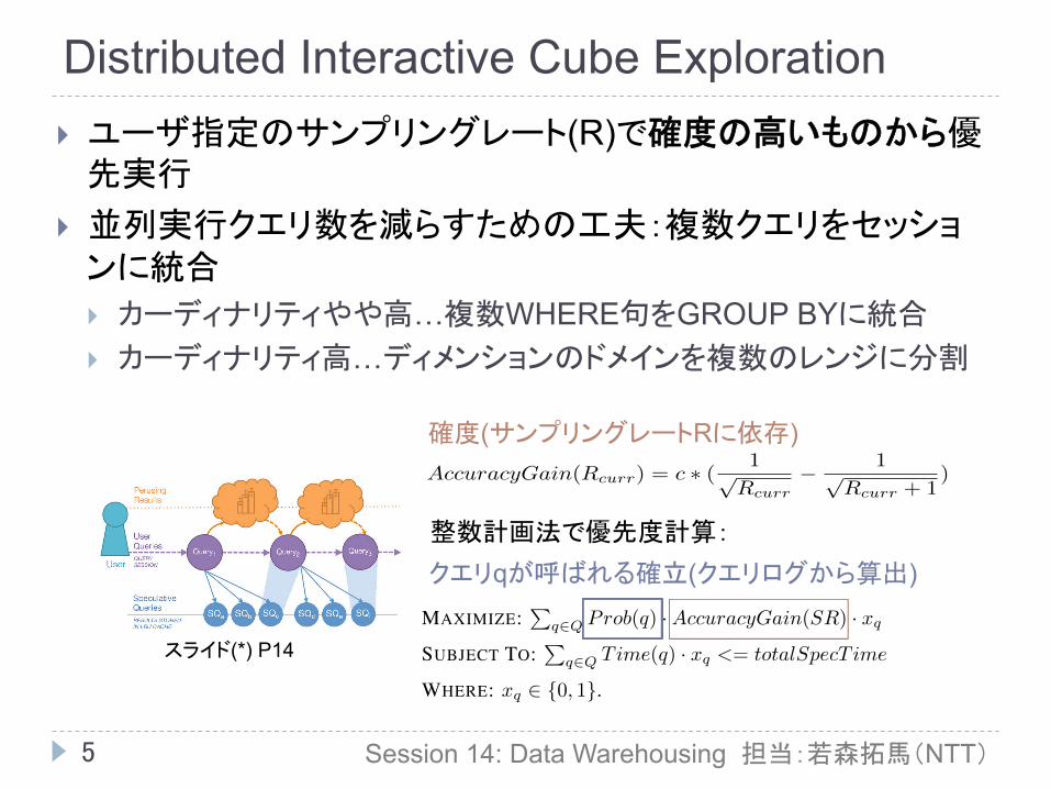
}  ユーザ指定のサンプリングレート(R)で確度の高いものから優先実行

}  並列実行クエリ数を減らすための工夫：複数クエリをセッションに統合 }  カーディナリティやや高…複数WHERE句をGROUP BYに統合 }  カーディナリティ高…ディメンションのドメインを複数のレンジに分割


B. System Architecture

The architecture of our system employs a hierarchicalmaster-slave approach, such that all queries are issued to themaster, and responded to by the master. In line with thesetting described in Section II-B, each slave manages multipletable shards. Each shard is atomic and read-only, and isimplemented as a table in a commodity relational database.The catalog of shards across all slave nodes is maintainedat the master. For a single exploration session, the catalog isused to ensure that the list of shards addressed is constant. Theslaves maintain an in-memory LRU cache for the results. In afast-changing database, table shards can be atomically addedand deleted from the slaves, and the master’s catalog can beupdated, allowing for querying over rapidly changing data.

C. Query Flow

The high-level query flow of DICE is as follows: eachad-hoc query is rewritten and federated to the slave nodes,where it is executed. The results are returned, aggregated andpresented to the user, along with the accuracy of the query.Upon success, a set of speculative queries is executed tillthe next user query is received, with the goal of increasingthe likelihood of caching as many of the future queries aspossible. When the successive ad-hoc query is issued, it isagain rewritten and federated, with the hope that its resultsare cached at the slaves at a high sampling rate, thus reducingthe latency of the overall ad-hoc query.

User Query: At startup, the master makes sure that allthe slaves are running and ready to accept queries. Onreceiving an ad-hoc query, the query is rewritten into multiplequeries, one per required random table shard and passed toeach slave. Since data is horizontally distributed across allslave nodes, the query itself is identical, with the exceptionof id of the table shard addressed. On completion of anad-hoc query (or if the results of the query were alreadyin the cache), each slave returns the results back to themaster, where the results are aggregated, and error calculationperformed, and this information presented to the user.

Speculative Queries: Upon completion of the ad-hocquery, the master immediately schedules a list of speculativequeries that can be issued by the user. While the space ofpossible queries is unbounded, we restrict our speculationsusing faceted exploration framework; thus allowing the listof possible queries to be enumerable. Speculated queries arethen ranked (as discussed in the following subsection), anddistributed amongst the slaves in a round-robin fashion. Eachslave issues, in an increasing order of rank, a predefinednumber of concurrent queries to its database and populatesthe results in its cache (speculative query results are not sentto the master). Upon receiving the next user query, the slavekills all currently running speculative queries.

Successive User Query: When the next ad-hoc queryarrives, it is again rewritten and federated to the slaves. If

the exact query or a unified query (refer to Section III-F) iscached, the result of the ad-hoc query is materialized fromthe cached result. If it is not cached it is then executed onthe database. The caching of speculated queries drasticallyimpacts ad-hoc query latency and allows for a fluid andinteractive data cube exploration experience.

D. Prioritizing Speculative Queries

As is clear from the query flow and the faceted model,each ad-hoc query can yield significantly large number ofspeculative queries. Given the bounded time available for exe-cution, it is typically not possible to execute all the speculativequeries. Thus, it is necessary to prioritize speculative queryexecution such that it maximizes the likelihood of results forthe successive query being returned from the cache. This canin turn be done by maximizing the overall gain in accuracy, asdiscussed in Section II-C. The selection of the maximal subsetcan be modeled as a linear integer programming problem asfollows:

MAXIMIZE:P

q2Q Prob(q) ·AccuracyGain(SR) · xq

SUBJECT TO:P

q2Q T ime(q) · xq <= totalSpecT ime

WHERE: xq 2 {0, 1}.

Here, Prob(q) gives the probability of a query q, whichshould be obtained from the query logs, Q is the set of allspeculative queries at all sampling rates, AccuracyGain(SR)is the estimated gain in sampling accuracy which dependson the sampling rate SR of q as described in Section II-C,T ime(q) is the estimated running time and totalSpecT imeis the expected total speculative time.

Considering the input parameters, it is not possible to solvethe above optimization problem in sub-second latency thuspreventing us from returning results within those latencies. Weexpect the majority of the query execution cost to be typicallydue to an in-memory table scan over identically sized dataif the table shards are pre-loaded in the memory. It is notpossible to load the entire dataset into memory but definitelya significant fraction which in our experiments was up to 20%such that the error bars for most of the groups were small.This lets us assume unit execution time for each query overa shard. In that case, it is clear that choosing the query thatyields the maximum of the product of the probability of aquery and the estimated accuracy gain for the correspondingsampling rate is the best decision. Therefore, the solution to theproblem of choosing of the best queries that yield the highestoverall accuracy gain turns into a greedy selection problem,the algorithm to which we provide in the following section.

Greedy Approach: The greedy cost-based approach priori-tizes the execution of the most likely queries that providethe highest overall accuracy gains. We represent the scoreof a query q at the sampling rate of SR as Prob(q) ·AccuracyGain(SR).

クエリqが呼ばれる確立(クエリログから算出)

スライド(*) P14

EFFECTIVENESS OF FACETED MODEL: The four traversalsmentioned above are both intuitive and sufficient to explorethe entire data cube. The parent, child and pivot traversals areinspired by rollup, drilldown and pivot operations respectively.It is always possible to add more traversal types, especiallyby mining a user’s query history for common “patterns”of analysis, e.g. keeping the bound dimensions the sameand changing the group by dimension. Such extensions areeasily pluggable into our system, but not required – the fourtraversals described above are intuitive and powerful enough totraverse the cube. We quantify the applicability of our modelon real-world query logs and measure user satisfactionusing a user study, described in Section IV-C.

B. Distributed Execution

The interactive nature of our use case necessitates theapproximation of results by executing queries over a subsetof the data. We use sharded tables to achieve distributedand sampled execution of queries. A sharded table containsa subset of the rows of a SQL table and the concatenationof all shards across nodes is equivalent to the entire dataset.Each node may contain multiple shards. A sharded table is theatomic unit of data in our system: updates are performed atthe granularity of the shard level, and each session makes theassumption that the list of shards and the shards themselvesdo not change.

C. Querying over Table Shards

A sample of the data is constructed online by choosingrandom table shards during run-time, allowing for randomsampling. We use standard sampling concepts of stratifiedsampling [13] and post-stratification [13] for estimating theerror bounds. Details on our use of sampling methods areprovided in the appendix.

Given the preliminaries and definitions, in the naive case,the problem of ad-hoc cube exploration using the facet ex-ploration model is simply that of successively executing eachquery received at a given sampling rate. We formulate ourproblem as the following:

For a facet session ~F , where each ad-hoc facet query fiis expected to execute at a certain sampling rate, and theexpected time between the termination of one facet query andthe start of the next ad-hoc facet query (i.e., the time taken toview the results of the prior query) is ⌧V , return fi as quicklyas possible to the end-user, preferably within the interactivethreshold ⌧I .

Accuracy Gain Heuristic: In order to schedule speculativequeries at different sampling rates, we need to know the reduc-tion in sampling error at different sampling rates. However, itcannot be known before actually sampling the data. Therefore,we construct a heuristic based on the consistency property ofMaximum Likelihood Estimation (MLE), ||✓⇤ � ✓|| = O( 1p

n)

where ✓⇤ is the current estimate, ✓ is the true value and n isthe current sampling rate, which informs us that the differencebetween our estimate and the true value will be inversely

proportional to the square root of the current sampling rate.Therefore, we can estimate the future gain in accuracy basedon the sampling rate. Thus, the estimated gain in the accuracydue to a unit sampling rate increase can be given as

AccuracyGain(Rcurr) = c ⇤ ( 1pRcurr

� 1pRcurr + 1

) (1)

where Rcurr is the current sampling rate and c is the constantfrom the proportionality heuristic.

With more time permissible, we issue the same query onmultiple tables on multiple nodes progressively giving usa smaller standard error for the estimators. Our goal thenduring speculative execution of the queries is to increase thelikelihood that the next user query would be cached at a highersampling rate allowing us to retrieve the results at the desiredsampling rate at the earliest. We cast this to fit the DICEframework in the following section.

III. THE DICE SYSTEM

A. Speculating Queries in a SessionA crucial insight to ad-hoc querying is that queries oc-

cur in sessions. Thus, it is prudent to think of improvingquery performance holistically at the session level. A sessioncomprises several ad-hoc queries, each of which requires low-latency responses. The result for each query is inspected bythe user for a small amount of time, after which the nextquery is issued. We consider this as a hidden opportunity –the database is simply waiting on the user to issue the nextquery. In light of this, our solution is to utilize this waitingtime to speculate, execute and cache the most likely followupqueries at the highest quality possible. While the concept ofspeculative execution is an intuitive one, there are severalchallenges to implementing it over a distributed, approximatequerying environment – especially in the context of data cubeexploration. The challenges comprise a host of interdependentproblems: What are the most likely followup queries? What isthe strategy to employ to execute and cache likely queries? Ina sampling approach, what is the highest sampling rate to runa speculative query at, given interactive constraints? Finally,is there a singular framework to combine these problems intoa cohesive, unified system?

Given these challenges, we present the DICE system thatsolves the problem by using three complementary strategies.First, it performs speculative query execution, by cachingresults of likely followup queries, allowing for reduced laten-cies for ad-hoc query sessions. The enumeration of the likelyfollowup queries is made possible by the faceted model ofdata cube exploration described in Section II. Second, DICEemploys a novel architecture of query execution over a dis-tributed database, executing queries piecemeal over individualtable shards and then assembling them in a post-processingstep. This novel architecture in turn allows for bounded-timeexecution of queries ensuring interactive latencies. Third, itemploys a cost-based model for the prioritized execution ofspeculative queries such that likely queries are executed athigher sampling rates.

整数計画法で優先度計算：

確度(サンプリングレートRに依存)

be speculated are selected randomly from the set of possiblefacet traversals. ALGOUNIFORM selects speculative queriesuniformly from each type of facet traversal. ALGODICEuses the DICE speculative query selection technique.ALGOPERFECT “improves” upon DICE by allowing for aperfect prediction of the subsequent ad-hoc query – thisrepresents the (hypothetical) best-case performance of ourspeculation strategy, and is included to demonstrate theoverall potential of speculative caching.

Metrics: AVERAGE LATENCY is measured in milliseconds asthe average latency of a query across sessions and runs. Wealso depict ±1 standard deviation of latency using error barsin most of our results. AVERAGE ACCURACY is measured asthe absolute percentage deviation of the sampled results fromthe results over the entire dataset.

B. Results

1) Impact of Data Size: We observe, in Figure 3 & 4, theimpact of data size on the latency observed by each algorithmby varying the target sample size for the ad-hoc queriesin our workload. ALGONOSPEC scales almost linearly, andexceeds the sub-second threshold for 200M rows. Despite issu-ing speculative queries, ALGORANDOM and ALGOUNIFORMperform just as poorly as ALGONOSPEC, validating the needfor a principled approach to speculative querying that DICEprovides. ALGODICE stays within the sub-second threshold,and scales quite well for increasing size, performing almost aswell as ALGOPERFECT (which is the lower bound for latencyin this case) and manages to maintain a near 100% cache hitratio, especially for smaller sampling rates. A 1-tailed t-testconfirms (p-value 0.05, t-statistic 58.41 > required criticalvalue 1.662) that ALGODICE’s speedup over ALGONOSPECis statistically significant. Another observation is a perfor-mance envelope with ALGOPERFECT exists – there are severalconstant-time overheads which could be further optimized,an opportunity for future work. Figure 4 performs the sameexperiment at a larger scale on CLUSTERCLOUD, allowing forcube exploration over the 1 billion rows (100% sampling)while maintaining a sub-second average latency – 33%faster than the baseline ALGONOSPEC.

2) Sampling & Accuracy: Since DICE allows the user tovary the sampling rate, we present a plot of the AVERAGEACCURACY for a sample workload, compared to results fromaggregation over the full dataset. It should be noted thataccuracy depends on multiple factors. First and foremost,accuracy is dependent on skew in the data. As described inthe schema, our dataset contains a multitude of distributionsacross all the dimensions. Second, the selectivity of queriesin the workload will impact the sensitivity of error. Third, theplacement of the data is a significant contributing factor: sincedata is horizontally sharded across multiple nodes, samplingand aggregation of data is impacted by the uniformity of dataplacement. In Figure 5, we present the average accuracy fora workload at varying sampling rates over all 1B rows. Forthis workload, accuracy increases steadily till the 50% mark,

after which the benefits of increasing the sampling taper off,slowly reaching full accuracy at the 100% sampling rate.

0"

200"

400"

600"

800"

1000"

1200"

1400"

1600"

1800"

0" 50" 100" 150" 200"

Time%(m

s)%

Sample%Size%(millions%of%rows)%

Cluster:)Small)

NOSPEC" Random" Uniform"

DICE" Perfect"

Fig. 3. Varying Size of Dataset: CLUSTERSMALL

250$ 500$ 750$ 1000$0$

200$

400$

600$

800$

1000$

1200$

1400$

1600$

Time%(m

s)%

Sample%Size%(millions%of%rows)%

Cluster:)Cloud)

NOSPEC$ DICE$ Perfect$

Fig. 4. Varying Size of Dataset: CLUSTERCLOUD

5" 10" 20" 50" 75" 100"40"

50"

60"

70"

80"

90"

100"

Accuracy'(%

)'

Sample'Size'(%)'

Cluster:)Small)Dataset:)1)billion)rows)

Fig. 5. Accuracy over a workload

0"

200"

400"

600"

800"

1000"

1200"

1400"

1600"

0" 2" 4" 6" 8" 10"

Time%(m

s)%

Number%of%Dimensions%

Cluster:)Small)

NOSPEC" DICE"

Fig. 6. Impact of Number of Dimensions

3) Number of Dimensions: Figure 6 shows how varying thenumber of dimensions in a query affects its execution time.

6

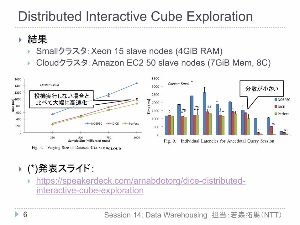
}  結果 }  Smallクラスタ：Xeon 15 slave nodes (4GiB RAM) }  Cloudクラスタ：Amazon EC2 50 slave nodes (7GiB Mem, 8C)

}  (*)発表スライド： }  https://speakerdeck.com/arnabdotorg/dice-distributed-

interactive-cube-exploration



Dimensions are increased by adding new WHERE predicatesto the query. As seen in Figure 6, execution time decreases upto a certain point and then starts increasing. The decreasingslope in the curve is caused by selectivity – as dimensionsare added, less number of rows are processed, allowing forfaster materialization of resultsets. After a certain point, theevaluation cost of the multiple WHERE clauses takes over,especially because the order of filter dimensions is not ideal.

4) Number of Slave Nodes: We vary the number of slavenodes in Figure 7, while keeping the size of the data constant at200M rows. As expected, for all algorithms, latencies decreaseas the number of nodes increases. An interesting observationis made for ALGODICE however – for 4 nodes, DICE thrashesmemory due to the amount of data involved and the numberof speculative queries, which is not a problem for bothALGONOSPEC (no speculation / caching) or ALGOPERFECT(exactly one ad-hoc query being cached).

0"

500"

1000"

1500"

2000"

2500"

3000"

3500"

2" 4" 6" 8" 10" 12" 14" 16"

Time%(m

s)%

Number%of%Nodes%

Cluster:)Small)

NOSPEC"DICE"Perfect"

Fig. 7. Varying the Number of Slave Nodes

40#50#60#70#80#90#100#

0# 50# 100# 150# 200#

Cache&Hit&R

ate&(%

)&

Sample&Size&(millions&of&rows)&

Cluster:)Small)

DICE#

Fig. 8. Cache Hit Change with Sampling Rate Change

5) Cache Hit Variability: Since the cache hit rate is a keycontributor to the average latency of a session, in Figure 8 westudy how the cache hit rate varies with the sampling rate fora fixed cache size. We use the cache hit rate as a proportionalmeasure of the prediction quality. Higher cache hits are a directresult of high quality of speculation. We achieve close to a100% hit rate for 50 million sampled rows. As we increasethe sampling rate, we see the cache hit rate decreasing nearlylinearly, since the total number of speculative queries increaseslinearly with the sampling rate.

6) Sample Session: As an anecdotal example, we presentin Figure 9 the trace of a single cube exploration ses-sion for ALGONOSPEC, ALGODICE and ALGOPERFECT onCLUSTERSMALL. The X axis depicts successive ad-hocqueries in a session. (It should be noted that while the bars arestacked together for convenience for the reader, the session foreach algorithm is executed separately.) The Y axis representsAVERAGE LATENCY. Cache hit rate for ALGODICE is shownas a label above the bars. The cache hit rate for the first query

0"

500"

1000"

1500"

2000"

2500"

3000"

3500"

Time%(m

s)% NOSPEC"

DICE"

Perfect"0 .75 .75 .68

1 1 1

1 .68

.75

Cluster: Small

Fig. 9. Individual Latencies for Anecdotal Query Session

is 0.0, since there has been no speculation and the caches areempty. ALGODICE performs almost as well as ALGOPERFECTwith hit rates equal or closer to 1.0.

7) Impact of Various Techniques: We now study in Fig-ure 10, the performance impact of the various algorithms andoptimizations to our system on the CLUSTERSMALL cluster.We compare the AVERAGE LATENCY of various techniquescompared to ALGONOSPEC. ALGOUNIFORM is slightly fasterdue to some of the speculative queries being part of thesession. Including the unification optimization discussed inSection III-F reduces the number of concurrent queries, im-proving latency. Finally, including the locality model and cost-based prioritization of speculative queries yields ALGODICE,which outperforms all other methods.

0"

500"

1000"

1500"

2000"

NOSPEC" UNIFORM" UNIFORM"+"BATCHING"

DICE"

Time%(m

s)%

Cluster:)Small ))

Fig. 10. Impact of Various Techniques

C. Real-world Usage and User StudyReal-world Query Logs: To evaluate the real-world efficacyof the facet model, we procured a real-world query log of ad-hoc analytical queries by real users on a production systemgenerated HIVE data warehouse of an Internet advertisingcompany. Considering only the aggregation queries (with thegroup by clause), the log spanned 509 queries. Amongstthem 46 query sessions were detected which comprised of 116queries i.e. 22.97% of the queries. The traversals described inthe DICE model were found to cover 100% of the session-based queries, demonstrating that our traversal model is in-deed expressive enough to allow for significant speedups (theremainder are executed traditionally, without speculation.)User Studies: We performed a user study to compare theeffectiveness DICE over traditional methods.The study wasperformed with 10 graduate students across the departmentwho were knowledgeable in databases and data cubing, deter-mined using a pre-test. The users were then given a pre-tasktutorial on data cubing and our data model. They were thenasked to explore the cube using the faceted model for 10 ad-hoc queries of their choice. They were not told if the DICEspeculation was turned on or off (50% of the users each).After the session, the user’s query session was repeated in the

投機実行しない場合と比べて大幅に高速化

分散が小さい

A Tunable Compression Framework for Bitmap Indices

7

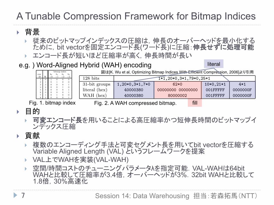
}  背景 }  従来のビットマップインデックスの圧縮は，伸長のオーバーヘッドを最小化する

ために，bit vectorを固定エンコード長(ワード長)に圧縮：伸長せずに処理可能 }  エンコード長が短いほど圧縮率が高く，伸長時間が長い

}  目的 }  可変エンコード長を用いることによる高圧縮率かつ短伸長時間のビットマップイ

ンデックス圧縮 }  貢献

}  複数のエンコーディング手法と可変セグメント長を用いてbit vectorを圧縮するVariable Aligned Length (VAL) というフレームワークを提案

}  VAL上でWAHを実装(VAL-WAH) }  空間/時間コストのチューニングパラメータλを指定可能．VAL-WAHは64bit

WAHと比較して圧縮率が3.4倍，オーバーヘッドが3%．32bit WAHと比較して1.8倍，30%高速化


2 · Kesheng Wu et al.

bitmap indexrow b0 b1 b2 b3ID X =0 =1 =2 =31 0 1 0 0 02 1 0 1 0 03 3 0 0 0 14 2 0 0 1 05 3 0 0 0 16 3 0 0 0 17 1 0 1 0 08 3 0 0 0 1

Fig. 1. A sample bitmap index. Each column b0 . . . b3 is called a bitmap in this paper.

empirical studies have shown that WAH compressed bitmap indices answer queriesfaster than uncompressed bitmap indices, projection indices, and B-tree indices, onboth high and low cardinality attributes [Wu et al. 2001; 2002; Stockinger et al.2002; Wu et al. 2004]. This paper complements the observations with rigorousanalyses. The main conclusion of the paper is that the WAH compressed bitmapindex is in fact optimal. Some of the most efficient indexing schemes such as B+-tree indices and B∗-tree indices have a similar optimality property [Comer 1979;Knuth 1998]. However, a unique advantage of compressed bitmap indices is thatthe results of one-dimensional queries can be efficiently combined to answer multi-dimensional queries. This makes WAH compressed bitmap indices well-suited forad hoc analyses of large high-dimensional datasets.

1.1 The basic bitmap index

In this paper, we define a bitmap index to be an indexing scheme that storesthe bulk of its data as bit sequences and answers queries primarily with bitwiselogical operations. We refer to these bit sequences as bitmaps. Figure 1 shows aset of such bitmaps for an attribute X of a hypothetical table (T), consisting ofeight tuples (rows). The cardinality of X is four. Without loss of generality, welabel the four values as 0, 1, 2 and 3. There are four bitmaps, appearing as fourcolumns in Figure 1, each representing whether the value of X is one of the fourchoices. For convenience, we label the four bitmaps as b0, . . . , b3. When processingthe query “select * from T where X < 2,” the main operation on the bitmapsis the bitwise logical operation “b0 OR b1.” Since bitwise logical operations arewell supported by the computer hardware, bitmap indices are very efficient [O’Neil1987].

The earlier forms of bitmap indices were commonly used to implemented in-verted files [Knuth 1998; Wong et al. 1985]. The first commercial product to makeextensive use of the bitmap index was Model 204 [O’Neil 1987]. In many data ware-house applications, bitmap indices perform better than tree-based schemes, suchas the variants of B-tree or R-tree [Jurgens and Lenz 1999; Chan and Ioannidis1998; O’Neil 1987; Wu and Buchmann 1998]. According to the performance modelproposed by Jurgens and Lenz [1999], bitmap indices are likely to be even morecompetitive in the future as disk technology improves. In addition to supportingqueries on a single table as shown in this paper, researchers have also demonstratedthat bitmap indices can accelerate complex queries involving multiple tables [O’Neil

ACM Transactions on Database Systems, Vol. V, No. N, July 2005.

8 · Kesheng Wu et al.

128 bits 1*1,20*0,3*1,79*0,25*1

31-bit groups 1,20*0,3*1,7*0 62*0 10*0,21*1 4*1

literal (hex) 40000380 00000000 00000000 001FFFFF 0000000F

WAH (hex) 40000380 80000002 001FFFFF 0000000F

Fig. 2. A WAH compressed bitmap. Each WAH word (last row) represents a multiple of 31 bitsfrom the input bitmap, except the last word that represents the four leftover bits.

Similar to WBC and BBC, WAH is also based on the basic idea of run-lengthencoding. However, unlike WBC or BBC, WAH does not use any header words orbytes, which removes the dependency mentioned above. In BBC, there are at leastfour different types of runs and a number of different ways to interpret a byte. InWAH, there are only two types of regular words: literal words and fill words. In ourimplementation, we use the most significant bit of a word to distinguish betweena literal word (0) and a fill word (1). This choice allows us to distinguish a literalword from a fill word without explicitly extracting any bit.

Let w denote the number of bits in a word, the lower (w−1) bits of a literalword contain the literal bit values. The second most significant bit of a fill word isthe fill bit (0 or 1), and the remaining bits store the fill length. WAH imposes theword alignment requirement on the fills; all fill lengths are integer multiples of thenumber of bits in a literal word, (w−1). For example, on a 32-bit CPU (w = 32),all fill lengths are integer multiples of 31 bits. In an implementation of a similarcompression scheme without word alignment, tests show that the version with wordalignment frequently outperforms the one without word alignment by two ordersof magnitude [Wu et al. 2001]. The reason for this performance difference is thatthe word alignment ensures logical operations only access whole words, not bytesor bits.

Figure 2 shows the WAH compressed representation of 128 bits. We assume thateach computer word contains 32 bits. Under this assumption, each literal wordstores 31 bits from the bitmap, and each fill word represents a multiple of 31 bits.The second line in Figure 2 shows the bitmap as 31-bit groups, and the third lineshows the hexadecimal representation of the groups. The last line shows the WAHwords also as hexadecimal numbers. The first three words are regular words, thefirst and the third are literal words and the second one is a fill word. The fill word80000002 indicates a 0-fill of two-word long (containing 62 consecutive 0 bits). Notethat the fill word stores the fill length as two rather than 62. The fourth word is theactive word, it stores the last few bits that could not be stored in a regular word1.

For sparse bitmaps, where most of the bits are 0, a WAH compressed bitmapwould consist of pairs of a fill word and a literal word. If the bitmap is truly sparse,say only one bit in 1000 is 1, then each literal words would likely contain a singlebit that is 1. In this case, for a set of bitmaps to contain N bits of 1, the total sizeof all compressed bitmap is about 2N words. In the next section, we will give arigorous analysis of sizes of compressed bitmaps.

1Note that we need to indicate how many bits are represented in the active word, and we havechosen to store this information separately (not shown in Figure 2). We also chose to store theleftover bits as the least significant bits in the active word so that during bitwise logical operationsthe active word can be treated the same as a regular literal word.

ACM Transactions on Database Systems, Vol. V, No. N, July 2005.

Fig. 1. bitmap index

図は[K. Wu et al, Optimizing Bitmap Indices With Efficient Compression, 2006]より引用

Fig. 2. A WAH compressed bitmap.

e.g. ) Word-Aligned Hybrid (WAH) encoding literal

fill


8

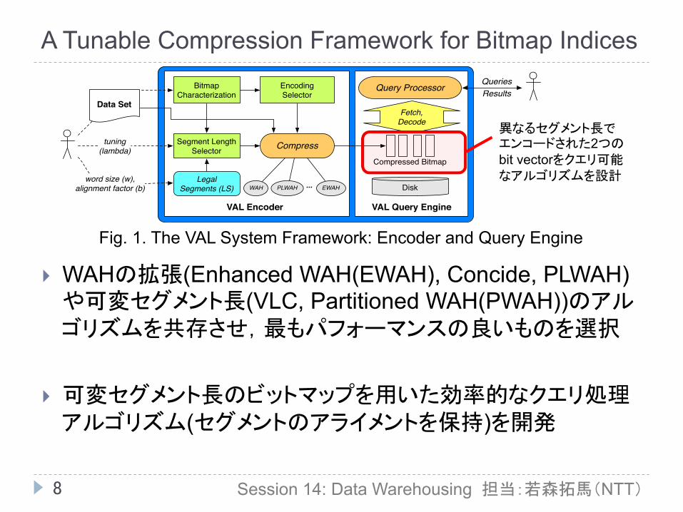
}  WAHの拡張(Enhanced WAH(EWAH), Concide, PLWAH)や可変セグメント長(VLC, Partitioned WAH(PWAH))のアルゴリズムを共存させ，最もパフォーマンスの良いものを選択

}  可変セグメント長のビットマップを用いた効率的なクエリ処理アルゴリズム(セグメントのアライメントを保持)を開発


LegalSegments (LS)

Bitmap Characterization

EncodingSelector

Segment LengthSelector Compress

VAL Encoder VAL Query Engine

Disk

Query Processor

Fetch,Decode

word size (w),alignment factor (b)

tuning(lambda)

QueriesResults

Data Set

WAH PLWAH EWAH

Compressed Bitmap

...

Fig. 1. The VAL System Framework: Encoder and Query Engine

Because tuples can be ordered arbitrarily in relations, re-ordering has been applied to maximize runs [18], [19], [20],[21], [22]. Finding an optimal order, however, has been shownto be NP-Complete [23], and different heuristics have beenproposed, such as lexicographic order, Gray codes [19], andHamming-distance-based [24], among others. Reordering pro-duces longer runs for the first few bit vectors, but generallydeteriorate into shorter runs (and worse, random noise) inthe higher dimensions. Such a pattern means that WAH canachieve optimal compression for the first few columns, butthe compression reduces for the later columns. This is themotivation for allowing varying segment lengths for each bitvector.

Previous efforts have also recognized the advantages inusing variable segment lengths for encoding. In VLC [13],arbitrary segment lengths can be used to encode each bit vector.Performance in query execution degrades drastically when seg-ment lengths are not aligned. Partitioned WAH (PWAH) [16]proposes to encode the bitmaps using several partitions withina 64-bit word. PWAH-8 for example, divides a word into8 partitions and stores fills and literals using 7 bits. PWAHmaintains a header in each word for all flag bits, enabling“extended fills”, using shorter block lengths to represent longerruns. However, PWAH does not propose to execute queriesinvolving bitmaps compressed using variable partition lengths.Since the partitions use unaligned segment lengths of 7, 15,or 31, queries involving bitmaps compressed with differentencoding lengths will require explicit decompression.

As expected, the use of these techniques is applicationand data-dependent. We have designed a unified compressionframework where these techniques can coexist and are used forthe cases where they can improve performance the most. Wedeveloped efficient query processing algorithms over bitmapscompressed using different segment lengths, while maintainingthe alignment of the segments. We have designed encodingand query processing interfaces that allow the integration ofvarious aligned run-length compression techniques. To informthe selection of the method/segment-length encoding to beused for a particular bitmap vector, we introduce a � parameterthat captures the trade-off between compression and decodingtime during query execution.

III. VARIABLE ALIGNED LENGTH (VAL) FRAMEWORK

Most modern bitmap compression techniques are variantsof the Word-Aligned Hybrid (WAH) encoding, which usesw-bit words to align with the underlying CPU architecture,e.g., w = 32 or w = 64. While the word size w is fixedon physical constraints, there is no such requirement that thesegment length s, i.e., the unit of compression, must be fixedat s = w � 1. Indeed, WAH-style fills and literals can easilybe represented in s = 7 bit segments, which is packed into thephysical unit of bytes rather than words[12].

The selection of the compression method, and indepen-dently, the segment length s, are both data and application-dependent. It is observable that there exists clear scenariosin which one method outperforms the others in time and/orspace. We have identified two orthogonal aspects that can begeneralized: (1) the encoding segment length s and (2) theencoding method used for compression. We propose a uni-fied bitmap compression framework, Variable Aligned Length(VAL), where these variations can coexist. Our frameworkinputs user preference on the space-time trade-off, and auto-matically applies the optimal settings to improve performance.

The proposed VAL system framework is shown in Figure1, comprising two main components: VAL Encoder and VALQuery Engine. The user inputs the data and a set of system-specific parameters. The input data set is first characterized,e.g., by profiling the overall bit distribution and length ofruns. This information is sent to the Encoding Selector and theSegment Length Selector. The former selector chooses an ap-propriate compression encoding scheme, and the latter decideson a segment length s to be used for encoding each bit vector.After compression, the compressed index is read by the VALQuery Engine which handles queries over the data set. Queriescan be executed over data compressed with different encodingtechniques or segment lengths. An important contribution ofthis paper is the design of querying algorithms that can operatetwo bit vectors encoded with different segment lengths. Thesealgorithms as well as the performance of the VAL Encoder areevaluated in Section V.

A. Bitmap Encoding CommonalitiesTo show the commonalities and generalizability of modern

WAH-variant schemes, let us focus on the encodings for sev-

Fig. 1. The VAL System Framework: Encoder and Query Engine

異なるセグメント長でエンコードされた2つの bit vectorをクエリ可能なアルゴリズムを設計


9

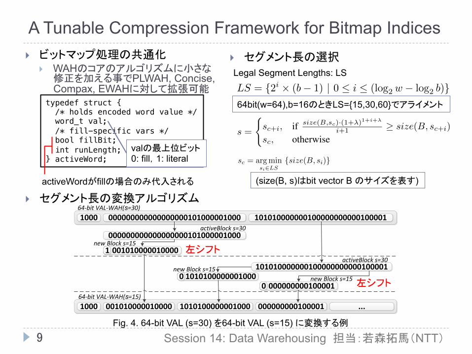
}  ビットマップ処理の共通化 }  WAHのコアのアルゴリズムに小さな

修正を加える事でPLWAH, Concise, Compax, EWAHに対して拡張可能


typedef struct { ! /* holds encoded word value */ ! word_t val; ! /* fill-specific vars */ ! bool fillBit; ! int runLength; !} activeWord; !

valの最上位ビット 0: fill，1: literal

1000 000000000000000000101000001000 101010000000100000000000100001

0010100000100001

000000000000000000101000001000

101010000000100000000000100001

1000 001010000010000

10101000000010000

1010100000001000

0000000001000010

000000000100001 ...

activeBlock s=30

new Block s=15

activeBlock s=30new Block s=15

new Block s=15

64-bit VAL-WAH(s=30)

64-bit VAL-WAH(s=15)

Fig. 4. Example of converting a 64-bit VAL compressed bit vector using s=30 down to a 64-bit VAL compressed bit vector using segment s=15.

• Case 1 (Lines 3-6): The alignedBlock is empty, i.e., thereare no bits left from the previous decoded block or word.If the activeBlock is a literal, then it is added to thealignedBlock as a literal and the alignedBlock is markedto be incomplete. The alignedBlock is not yet added tothe activeWord.

• Case 2 (Lines 7-11): The alignedBlock is empty and theactiveBlock is a fill, then its fill is added to allignedWordwith a factor of m less nSegments. The alignedBlockused to store the remainder bits from the division by m.They are stored as s bits in a literal.

• Case 3 (Lines 12-18): The alignedBlock is not empty,i.e., there are leftover literal bits from a previous block,and activeBlock is also a literal. In this case, the active-Block is appended to alignedBlock. If the alignedBlock isfilled with s⇥m bits, then it is added to the activeWordand cleared.

• Case 4 (Lines 19-25): The alignedBlock is a literal andactiveBlock is a fill. In this case, the alignedBlock isappended with literals from the activeBlock until it isfilled with s ⇥ m bits. The alignedBlock is appendedto activeWord as a literal block. Then the remainingblocks in activeBlock are appended to activeWord asa fill. If there are any leftover bits from dividing theremaining blocks by m, then they are stored as a literalin alignedBlock.

Aligning blocks with different compression lengths posesa small overhead in the VAL query processing algorithm.However, in general, VAL compresses better and often requiresfewer iterations to complete the query, as described in Algo-rithm 1. This translates into performance benefits not only interms of compression ratio, but also in terms of total querytime execution when compared to WAH.

V. EXPERIMENTAL RESULTS

In this section, the performance of VAL bitmap compressionframework is evaluated over both real scientific and syntheti-cally generated data. We first describe the experimental setupand the data sets used. Then we show the effectiveness ofthe tuning parameter � to trade-off size against query timeand then evaluate the impact on performance of the alignmentimposed over the segment lengths by comparing to VariableLength Coding (VLC). We then compare the performance of

Algorithm 3: A Method for Decoding Up (p < 0).Input: Compressed word containing blocks of length s; N : the number

of blocks in the word; possible values 1,2, m = 2|p|: factor ofthe new segment length

Output: activeWord - VAL Word containing decoded blocks oflength s⇥m

1 for i = 1 ! N do2 activeBlock= i’th block;3 if alignedBlock.nSegments=0 then4 if activeBlock.isLiteral() then5 alignedBlock.addLiteral(activeBlock.value)6 end7 else8 activeWord.addFillBlock(activeBlock.fill,

activeBlock.nSegments/m);9 store the leftover bits in alignedBlock, if any

10 end11 end12 else13 if activeBlock.isLiteral() then14 alignedBlock.addLiteral(activeBlock.value);15 if alignedBlock.isComplete() then16 activeWord.addLiteralBlock(alignedBlock.value)

alignedBlock.clear()17 end18 end19 else20 while alignedBlock.isNotComplete() do21 alignedBlock.addLiteral(activeBlock.fill)

activeBlock.nSegments- -22 end23 activeWord.addLiteralBlock(alignedBlock)

alignedBlock.clear()activeWord.addFill(activeBlock.fill,activeBlock.nSegments/m) store the leftover bits inalignedBlock, if any

24 end25 end26 end27 return activeWord

VAL-WAH on sorted bitmaps with other bitmap compres-sion schemes: Position List Word Aligned Hybrid (PLWAH),Enhanced Word Aligned Hybrid (EWAH), and Word AlignedHybrid (WAH). Finally, we introduce a Gain metric computedas the harmonic mean of compression and query time ratios(normalized using the performance for verbatim or uncom-pressed bitmaps) to evaluate the combined performance.

}  セグメント長の選択

in LS. For example, for b = 8 and w = 64, the legal segmentlength s = 56 would have 7 unused bits per word. However, itis worth noting that in many cases the increase in compressionfor the bit vectors encoded with smaller segment lengths willmake up for these pad bits in the bit vectors encoded withlarger segment lengths.

Let us consider again the system framework presented inFigure 1. Along with the data set, the user also inputs themachine’s word size w, the alignment factor b, and a tuningparameter � (explained later). First, w and b are input intoEquation 1 to determine the set of legal segment lengths, LS.Next, encoding a bitmap involves two major decisions: (1)the encoding method to use, and (2) the segment length s 2LS. To inform on these decisions, the Bitmap Characterizationcomponent passes over and profiles each bit vector from theinput data. This profile is used as input into both the EncodingSelector and the Segment Length Selector.

The Encoding Selector determines an encoding for a bitvector given its profile. For example, if the bit vector isvery sparse, then PLWAH may be selected. EWAH may bepreferred for noisy bitmaps that have a majority of literalsand short fills. The Segment Length Selector uses the profileand LS to identify an appropriate s 2 LS to compresseach bit vector. In general, bitmaps compressed using smallersegments will compress more aggressively, but may requiremore decoding and bookkeeping operations when executingqueries. To exploit this trade-off, we allow users to input atuning parameter �, 0 � 1. As � approaches 0, thesystem will attempt to achieve the best compression possible,while a � approaching 1 prioritizes faster query execution time.

Given a bit vector B and �, the Segment Length Selectorwill return

s =

(sc+i

, if size(B,sc)·(1+�)1+i+�

i+1 � size(B, sc+i

)

sc

, otherwise(2)

where size(B, s) is the size of the bit vector B when com-pressed with segment length s. The term,

sc

= argmin

si2LS

{size(B, si

)} (3)

refers to the segment length that yields the most compressedbit vector. Similarly, s

c+i

denotes the ith legal segment lengthgreater than s

c

in LS.After these parameters are selected, B is compressed. A

header byte must be appended to the beginning of eachcompressed bit vector. The most significant four bits in theheader are used to identify the multiplier m for the alignmentfactor b, such that (m⇥b) 2 LS is the selected segment length.The remaining four bits encodes the method used, e.g., WAHor PLWAH.

D. The VAL Query EngineEnabling variable segment lengths complicates query pro-

cessing. As discussed previously, queries are executed byperforming logical bitwise operations between bit vectors. Ingeneral, the more compressed blocks are contained in the bitvector, the longer it takes to execute the query as compressed

blocks need to be decoded. Using variable segment lengthscan increase decoding costs. However, in the cases where bothbitmaps are compressed well, there are opportunities for fasterquery execution by processing whole compressed blocks.

In our framework, two VAL bit vectors Xm⇥s

and Ys

encoded using segment lengths m⇥ s and s, respectively areoperated together to produce bit vector Z

s

, which stores theresult of the bitwise logical operation X

m⇥s

�Ys

, where � is abinary logical operator. Algorithm 1 shows the pseudocode forquery processing. Each bitmap is still decoded one physicalword (currentWord) at a time (Line 1-7). The parameter m(Line 3) indicates that the currentWord should be decodedinto blocks of segment length m ⇥ s. The decoded current-Word contains a number of activeBlocks. This activeBlock istantamount to the activeWord structure used in WAH. ThecurrentWords are iterated one block at a time (Lines 8-14)and are operated together until exhausted. Two fill blocks canbe operated without explicit decompression (Lines 15-20). Ifone of the activeBlocks is a literal, then the values are operatedtogether and the number of segments in the fill, nSegments, isdecremented by 1 with each getLitValue() call (Lines 21-23).

Algorithm 1: General Bitwise Logical OperationInput: Bit Vector X , Y : (X .segLen=m⇥ s and Y .segLen=s)Output: Bit Vector Z: The resulting compressed bit vector after

performing the logical operation X � Y

1 while X and Y are not exhausted do2 if X .currentWord is exhausted and there are more words in X then3 X .decodeNextWord(m);4 end5 if Y .currentWord is exhausted and there are more words in Y then6 Y .decodeNextWord(1);7 end8 while X .currentWord and Y .currentWord are not exausted do9 if X .activeBlock.nSegments = 0 then

10 X .activeBlock = X .nextBlock();11 end12 if Y .activeBlock.nSegments == 0 then13 Y .activeBlock = Y .nextBlock();14 end15 if X .activeBlock.isFill() and Y .activeBlock.isFill() then16 nSegments = min(X .activeBlock.nSegments,17 Y .activeBlock.nSegments);18 Z.addFill(X .activeBlock.fill19 � Y .activeBlock.fill, nSegments);20 X .activeBlock.nSegments -= nSegments;21 Y .activeBlock.nSegments -= nSegments;22 end23 else24 Z.addLiteral(X .activeBlock.getLitValue()25 � Y .activeBlock.getLitValue());26 end27 end28 end29 return Z;

Note the similarities between Algorithm 1 and the WAHprocessing algorithm described in Section III-A. The encoding-specific details are enabled through implementing the abstractmethod decodeNextBlock(). As a proof-of-concept, we imple-mented WAH within our generalized framework and optimizedquery execution over variable segment lengths.

is exhausted. At this point, the next word is read from thecache and decoded. An activeWord can be interpreted as thefollowing structure,typedef struct {

/* holds encoded word value */word_t val;/* fill-specific vars */bool fillBitint runLength;

} activeWord;

where sizeof(word_t) is equal to the machine’s word size.The encoded value of the word is stored in val, and todetermine whether an activeWord is a fill or literal is doneby simply examining val’s most significant bit. Clearly, thevalues of fillBit and runLength are only assigned if theactiveWord is determined to be a fill.

There are three cases when executing the AND between thetwo activeWords, X and Y. (Case 1) If X and Y are both fills, theresult is a new fill word with its fillBit equal to the result ofX.fillBit & Y.fillBit. The new fill word’s runLengthis assigned abs(X.runLength-Y.runLength). (Case 2) If Xand Y are both literals, then the result is a new literal word withval set to X.val & Y.val. (Case 3) Finally, if X is a literaland Y is a fill, then the number of segments in the fill wordis first decremented by one: Y.runLength--. Afterwards, theresult is a new literal word with val being set to the & resultbetween X.val and the literal value of Y.fillBit. Bit vectorsare never explicitly decoded one bit at a time. Considering eachbit as a processing unit, operations of type (Case 1) observe asuperlinear speedup, while operations of type (Case 2 and Case3) observe an s⇥ speedup, where s is the encoded segmentlength.

Due to the shared encoding similarities of the WAH variants,we observe that WAH’s core processing algorithm can alsobe easily extended to process PLWAH, Concise, Compax, orEWAH with minor modifications. For PLWAH and Concise,decoding of the activeWord word could produce one fill andone literal when the position bits for the fill are not all zeros.This literal is the word either following or preceding the fill,respectively for PLWAH and Concise. The logic for queryprocessing remains similar; the difference is to operate boththe dirty literal and the fill before decoding the next word.

To query using Compax, there will be more branch opera-tions, because it uses four types of words. For fill words, moredecoding is required to decide whether the fill is of the formFill-Literal-Fill (FLF) or Literal-Fill-Literal (LFL). In thosecases, three active words will be created but the query pro-cessing logic still remains the same. The branching overheadis the trade-off for Compax’s update friendly structure.

Because EWAH applies a different encoding for the fills, itdoes not generate multiple activeWords after decoding. It onlystores the number of literal words following the fill, and thisinformation is used for query optimization. When two fills areANDed together and one of them is a zero fill, literal wordscan be skipped without decoding by incrementing the positionof the vector iterator. Also, literals can be ANDed until thecounter reaches zero without requiring any decoding. Thesetranslate into faster query execution. Nevertheless, the logic for

operating literals and fill values remains relatively unchanged.

C. The Val EncoderTo generalize query processing over variable segment

lengths, we introduce a more general activeBlock in lieu ofan activeWord. An activeBlock shares the basic structure ofan activeWord, except that the activeBlock.val considerssequences of s (s w) bits. When s = w, there is oneblock per word, and the structures and query processing reduceback to the original algorithm. However, for encodings usingsmaller segment lengths s < w, decoding of a physical word,would produce two or more activeBlocks. For example, whenw = 64, s = 15, there would be four activeBlocks perphysical word.

The goal of our framework is to improve compressionwithout adversely affecting query performance. For this reason,the segment lengths s cannot be arbitrary, as we would lose thealignment benefits. Queries would suffer from considerable de-coding overhead during query execution. Given the machine’sword size w and an alignment factor b, b w, we define theset of Legal Segment Lengths LS as,

LS = {2i ⇥ (b� 1) | 0 i (log2 w � log2 b)} (1)

On a 64-bit architecture (w = 64) and alignment factorb = 16, the legal segment lengths are, LS = {15, 30, 60}.This definition of segment lengths ensures that larger segmentlengths are always multiple of smaller segment lengths, andtherefore the activeBlocks they create are always logicallyaligned. To further reduce the overhead of query execution,the segments are also memory-aligned, i.e., segments nevercross over two physical words. For instance, segment lengthss = 15, 30, and 60 encapsulate four, two, and one block(s)into a single physical word, respectively. When needed, blocksare padded with zeros within the physical word. For example,recall that each block is encoded using s+1 bits (the one extrabit is needed to flag the block as being either a literal or a fill).

Fig. 3. Word Encapsulation

This word encapsulation scheme is shown in Figure 3. Thenumber of blocks encapsulated into a word is given by N =

(b�1)⇥w

b⇥s

. The flag bit for each block is stored in the w

b

-bit wordheader. The goal of the word header is to minimize the timerequired to align the segments between two bitmaps encodedusing different block sizes. For example, two literal blockswith a VAL bitmap encoded using s = 15 can be directlyoperated with the corresponding literal block encoded usings = 30. It is worth noting that small alignment factors wouldhave a significant number of unused bits for larger segments

in LS. For example, for b = 8 and w = 64, the legal segmentlength s = 56 would have 7 unused bits per word. However, itis worth noting that in many cases the increase in compressionfor the bit vectors encoded with smaller segment lengths willmake up for these pad bits in the bit vectors encoded withlarger segment lengths.

Let us consider again the system framework presented inFigure 1. Along with the data set, the user also inputs themachine’s word size w, the alignment factor b, and a tuningparameter � (explained later). First, w and b are input intoEquation 1 to determine the set of legal segment lengths, LS.Next, encoding a bitmap involves two major decisions: (1)the encoding method to use, and (2) the segment length s 2LS. To inform on these decisions, the Bitmap Characterizationcomponent passes over and profiles each bit vector from theinput data. This profile is used as input into both the EncodingSelector and the Segment Length Selector.

The Encoding Selector determines an encoding for a bitvector given its profile. For example, if the bit vector isvery sparse, then PLWAH may be selected. EWAH may bepreferred for noisy bitmaps that have a majority of literalsand short fills. The Segment Length Selector uses the profileand LS to identify an appropriate s 2 LS to compresseach bit vector. In general, bitmaps compressed using smallersegments will compress more aggressively, but may requiremore decoding and bookkeeping operations when executingqueries. To exploit this trade-off, we allow users to input atuning parameter �, 0 � 1. As � approaches 0, thesystem will attempt to achieve the best compression possible,while a � approaching 1 prioritizes faster query execution time.

Given a bit vector B and �, the Segment Length Selectorwill return

s =

(sc+i

, if size(B,sc)·(1+�)1+i+�

i+1 � size(B, sc+i

)

sc

, otherwise(2)

where size(B, s) is the size of the bit vector B when com-pressed with segment length s. The term,

sc

= argmin

si2LS

{size(B, si

)} (3)

refers to the segment length that yields the most compressedbit vector. Similarly, s

c+i

denotes the ith legal segment lengthgreater than s

c

in LS.After these parameters are selected, B is compressed. A

header byte must be appended to the beginning of eachcompressed bit vector. The most significant four bits in theheader are used to identify the multiplier m for the alignmentfactor b, such that (m⇥b) 2 LS is the selected segment length.The remaining four bits encodes the method used, e.g., WAHor PLWAH.

D. The VAL Query EngineEnabling variable segment lengths complicates query pro-

cessing. As discussed previously, queries are executed byperforming logical bitwise operations between bit vectors. Ingeneral, the more compressed blocks are contained in the bitvector, the longer it takes to execute the query as compressed

blocks need to be decoded. Using variable segment lengthscan increase decoding costs. However, in the cases where bothbitmaps are compressed well, there are opportunities for fasterquery execution by processing whole compressed blocks.

In our framework, two VAL bit vectors Xm⇥s

and Ys

encoded using segment lengths m⇥ s and s, respectively areoperated together to produce bit vector Z

s

, which stores theresult of the bitwise logical operation X

m⇥s

�Ys

, where � is abinary logical operator. Algorithm 1 shows the pseudocode forquery processing. Each bitmap is still decoded one physicalword (currentWord) at a time (Line 1-7). The parameter m(Line 3) indicates that the currentWord should be decodedinto blocks of segment length m ⇥ s. The decoded current-Word contains a number of activeBlocks. This activeBlock istantamount to the activeWord structure used in WAH. ThecurrentWords are iterated one block at a time (Lines 8-14)and are operated together until exhausted. Two fill blocks canbe operated without explicit decompression (Lines 15-20). Ifone of the activeBlocks is a literal, then the values are operatedtogether and the number of segments in the fill, nSegments, isdecremented by 1 with each getLitValue() call (Lines 21-23).

Algorithm 1: General Bitwise Logical OperationInput: Bit Vector X , Y : (X .segLen=m⇥ s and Y .segLen=s)Output: Bit Vector Z: The resulting compressed bit vector after

performing the logical operation X � Y

1 while X and Y are not exhausted do2 if X .currentWord is exhausted and there are more words in X then3 X .decodeNextWord(m);4 end5 if Y .currentWord is exhausted and there are more words in Y then6 Y .decodeNextWord(1);7 end8 while X .currentWord and Y .currentWord are not exausted do9 if X .activeBlock.nSegments = 0 then

10 X .activeBlock = X .nextBlock();11 end12 if Y .activeBlock.nSegments == 0 then13 Y .activeBlock = Y .nextBlock();14 end15 if X .activeBlock.isFill() and Y .activeBlock.isFill() then16 nSegments = min(X .activeBlock.nSegments,17 Y .activeBlock.nSegments);18 Z.addFill(X .activeBlock.fill19 � Y .activeBlock.fill, nSegments);20 X .activeBlock.nSegments -= nSegments;21 Y .activeBlock.nSegments -= nSegments;22 end23 else24 Z.addLiteral(X .activeBlock.getLitValue()25 � Y .activeBlock.getLitValue());26 end27 end28 end29 return Z;

Note the similarities between Algorithm 1 and the WAHprocessing algorithm described in Section III-A. The encoding-specific details are enabled through implementing the abstractmethod decodeNextBlock(). As a proof-of-concept, we imple-mented WAH within our generalized framework and optimizedquery execution over variable segment lengths.

64bit(w=64),b=16のときLS={15,30,60}でアライメント

(size(B, s)はbit vector B のサイズを表す)

Fig. 4. 64-bit VAL (s=30) を64-bit VAL (s=15) に変換する例

左シフト

左シフト

activeWordがfillの場合のみ代入される

}  セグメント長の変換アルゴリズム

Legal Segment Lengths: LS


10 Session 14: Data Warehousing 担当：若森拓馬（NTT）

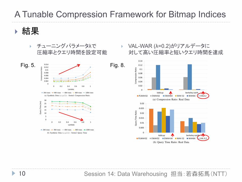
}  結果 data as for synthetically generated data. VAL-WAH offers thebest compression and better query time than WAH32. EWAHhas the best performance in terms of query time, howeverthis is mostly due to a difference in implementation. In ourexperiments we used ArrayLists for storing the bit vectors inall encoding techniques except EWAH. For EWAH, we comparedusing the implementation offered by [18].

0

0.02

0.04

0.06

0.08

0.1

0.12

0.14

kddcup berkeley earth

Com

pres

sion

Ratio

PLWAH32 EWAH32 EWAH64 WAH 32 WAH64 VAL0.2

(a) Compression Ratio: Real Data

0

0.005

0.01

0.015

0.02

0.025

0.03

kddcup berkeley earthQ

uery

Tim

e Ra

tioPLWAH32 EWAH32 EWAH 64 WAH 32 WAH64 VAL 0.2

(b) Query Time Ratio: Real Data

Fig. 8. Compression and Query Time Ratio Comparison - Real Data: Sorted

To help simplify the discussion on trade-off, we combinecompression ratio and query time ratio into a single metric,gain. Presuming that speedup and compression rates areequally weighed, we can use the harmonic mean H

M

of thetwo ratios,

gain =

1

HM

=

query ratio+ compression ratio

2⇥ query ratio⇥ compression ratio

Because the harmonic mean emphasizes the smaller ratio, itcaptures the combined rate of speedup and compression morefaithfully than an arithmetic mean. Furthermore, we invertedH

M

so that the larger values imply better performance, and thegoal would be to show higher gain. The gain across all datasets is presented in Figure 9. The combined gain of VAL-WAHis higher than the other encoding methods.

E. Results over Non-Sorted DataAlthough the motivation for encoding bitmaps using differ-

ent segment lengths came from observations of the run-lengthdeterioration for sorted data, performance gains can also beobtained for non-sorted data, as seen in Figure 10. In this case,EWAH is clearly the best encoding, followed by VAL0.2. Thisis due to a better query execution time given that EWAH uses

Fig. 9. Combined Gain for Sorted Bitmaps

Arrays for storing the bit vectors, while all the other techniquesuse ArrayLists. Because runs are very short, neither WAH norPLWAH are able to compress very effectively.

Fig. 10. Combined Gain for Non-sorted Bitmaps

Fig. 11. Combined Gain for Non-sorted Bitmap over Cardinality

To evaluate the effect of cardinality on gain, we generateda zipf1 data set with 10 million rows and two attributes ofincreasing cardinality from 10 to 10K values. Figure 11 showsthe gains obtained from this experiment. Larger cardinalityproduces bitmaps that are more sparse. As expected, EWAHhas the smallest gain, followed by WAH. The reason is that, forsparse bitmaps, EWAH does not compress as effectively as WAH,and the query times are not much better than those of WAH.Because VAL0.2 and PLWAH are able to compress better, in

A. Experimental SetupThe synthetic data sets were generated using two different

distributions: uniform and zipf. These two distributionsare representative of real-world bitmaps because continuousattributes and even high cardinality attributes are transformedusing discretization (or binning) before creating the bitmapindices. The distribution of the data into bitmap indices de-pends on the method used for discretization. For example, ifequi-populated bins (containing roughly the same number ofobjects) are used, the distribution of the bitmaps is uniform.However, if the discretization method is based on clustering,or on the density of data, then the bins would follow a skeweddistribution. The zipf distribution generator assigns each bit aprobability of,

p(k, n, f) =1/kfP

n

i=1(1/if

)

where n is the number of elements determined by cardinality,k is their rank, and the coefficient f creates an exponentiallyskewed distribution. We generated data sets for f = 1 andf = 2.

Unless otherwise noted, the synthetic bitmap index contains10 million rows and 100 bit vectors (4 attributes each with abinning cardinality of 25). We also included two real data setsin our experiments:• kddcup1. This data set was used for The Third

International Knowledge Discovery and Data MiningTools Competition, which was held in conjunction withKDD’99. The data set contains 4, 898, 431 rows and 42

attributes. Continuous attributes were discretized into 25

bins.• berkeley earth2. The Berkeley Earth Surface Tem-

perature Study has created a preliminary merged data setby combining 1.6 billion temperature reports from 16

preexisting data archives. For our experiments we usea subset containing 14, 786, 160 rows and 7 attributes.Each attribute was discretized with up to 25 bins.

Discretization over these real data sets was done using the leastsquares quantization method [25]. For sorted data experiments,Gray-code ordering [19] was used to reorder the bitmaps.

All experiments were executed over a machine with an IntelCore i7-2600 processor (8MB Cache, 3.20 GHz) and 8 GBof memory, running Windows 7 Enterprise. Our code wasimplemented in Java for relative performance measurementswith open-source implementations of EWAH and Concise.

A set of 500 queries over two randomly selected columns(from different attributes) was generated. Each query appliesa logical AND over the corresponding bitmaps. For queryexecution time, we do not take into account the time requiredto load the bitmaps into memory. Note that comparatively, thispresents an advantage for the techniques that produce largerbitmaps (EWAH and WAH64). However, since all bitmapsfit into main memory, loading time can be done once andamortized over a large number of queries. The query set was

1http://archive.ics.uci.edu/ml/datasets/KDD+Cup+1999+Data2http://berkeleyearth.org/dataset/

executed six times, and the result for the first run was discardedto prevent Java’s just-in-time compilation from skewing results.The times from the other five runs were averaged and reported.

For all experiments, we assume w = 64 bits, the alignmentfactor b = 16, and � parameter is set between 0 and 1

to choose among s 2 {15, 30, 60}. The query processinginvolving two bitmap vectors encoded using different segmentlengths would convert the larger encoding down to the smallerone, as presented in Algorithm 2.

B. Tuning Parameter �

The parameter � allows users to tune the aggressiveness ofour compression technique. Specifically, � ! 0 prioritizes onthe index size, while � ! 1 prioritizes speed.

00.0020.0040.0060.008

0.010.0120.014

0 0.2 0.4 0.6 0.8 1

Com

pres

sion

Ratio

Lambda

2M-rows 4M-rows 6M-rows 8M-rows 10M-rows(a) Synthetic Data (zipf2) - Sorted: Compression Ratio

0

5

10

15

20

25

30

0 0.2 0.4 0.6 0.8 1

Que

ry T

ime

(ms)

Lambda

2M-rows 4M-rows 6M-rows 8M-rows 10M-rows

(b) Synthetic Data (zipf2) - Sorted: Query Time

Fig. 5. VAL: Effects of � on Compression and Query Time: Synthetic Data

Figure 5 shows the effect of � over the compression ratioand query time for a synthetic sorted data set with zipf-2distribution. Figure 5(a) shows the compression ratio as � isvaried from 0 to 1 by increments of 0.2. The compression ratiois computed as size

compressed

/sizeverbatim

. As expected,compression ratio increases (i.e., we lose compression) as �increases, which translates into faster query times as capturedin Figure 5(b). Similar results were also observed for the realdata sets and for non-sorted data.

When � = 0.0, VAL uses the smallest segment length (s =15) for encoding over 70% of the columns, which reduces tolittle over 20% for � = 0.8. Increasing � allows more columns

}  VAL-WAR (λ=0.2)がリアルデータに対して高い圧縮率と短いクエリ時間を達成

}  チューニングパラメータλで圧縮率とクエリ時間を設定可能

Fig. 5. Fig. 8.

Pagrol: Parallel Graph OLAP over Large-scale Attributed Graphs

11

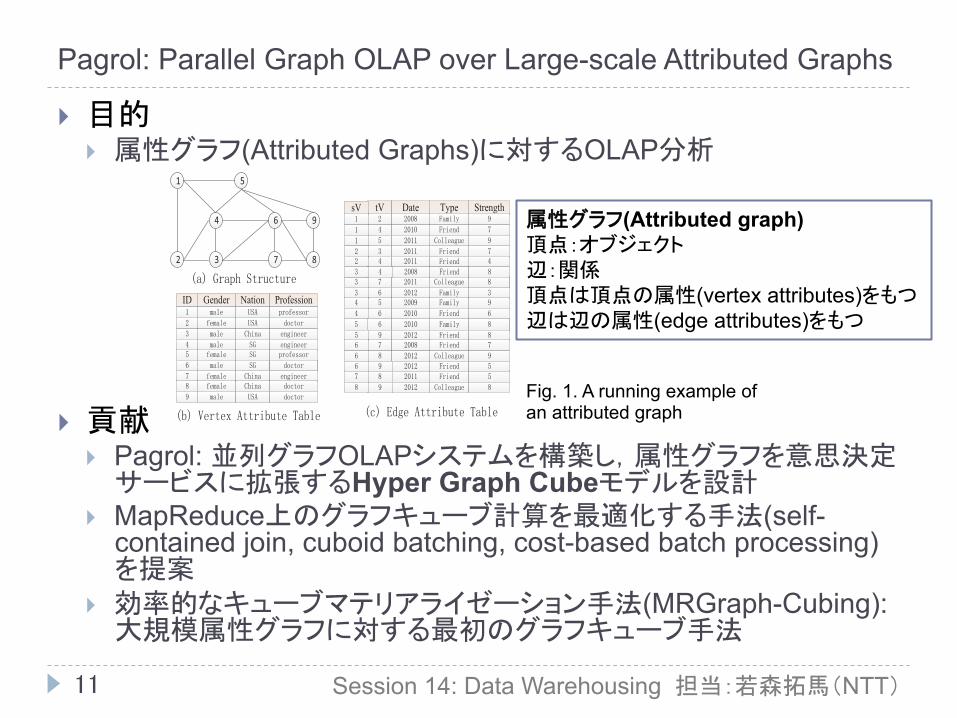
}  目的 }  属性グラフ(Attributed Graphs)に対するOLAP分析

}  貢献 }  Pagrol: 並列グラフOLAPシステムを構築し，属性グラフを意思決定

サービスに拡張するHyper Graph Cubeモデルを設計 }  MapReduce上のグラフキューブ計算を最適化する手法(self-

contained join, cuboid batching, cost-based batch processing)を提案

}  効率的なキューブマテリアライゼーション手法(MRGraph-Cubing): 大規模属性グラフに対する最初のグラフキューブ手法


deployed to speed up OLAP query processing in RDBMS[2]. However, traditional data cube model is not applicableto graphs as it does not capture the graph structures. Thus, weneed to design a conceptual graph cube model that supports thequeries in all the three categories. Second, for large attributedgraphs, parallelism is an effective and promising approach toensure acceptable response time. As such, we seek to developscalable parallel solutions for evaluating queries representedunder our graph cube model.

Recently, numerous distributed graph processing systemshave been proposed, such as Pregel [3], GraphLab [4], Pow-erGraph [5]. These systems are vertex-centric and follow abulk synchronous parallel model (where vertices send mes-sages to each other through their connections or IDs). Theyare tailored and efficient for graph processing operators thatrequire iterative graph traversal, such as page rank, shortestpath, bipartite matching and semi-clustering[3]. However, it iscostly to support graph cube computation. In fact, it will incurhigh overhead for message (carrying the attributes values)passing across the graph to find the vertices/edges with thesame attribute values. Compared to vertex-centric processingmodel, the MapReduce (MR) computation paradigm has beenshown to be efficient and scalable in supporting aggregate-like operators which do not require multiple iterations [6].As we shall see later, graph cube computation is exactlysuch an operator. As such, MR, which has been successfullydemonstrated to be effective for large graph mining [7][8],turns out to be a better fit for OLAP cube computation.

We are thus motivated to develop a new graph OLAPand warehousing model over attributed graphs as well as todevelop parallel graph OLAP system over MR that is able tosupport an efficient graph cube computation algorithm. Ourmajor contributions are summarized as follows:

• We propose a parallel graph OLAP system, Pagrol, toprovide a good decision making support over large-scale attributed graphs. To support graph OLAP, Pa-grol adopts a new conceptual graph cube model, HyperGraph Cube, to extend decision making services onattributed graphs. Hyper Graph Cube is able to capturequeries of all the aforementioned three categories intoone model. Moreover, the model supports a new setof OLAP Roll-Up/Drill-Down operations on attributedgraphs.

• We propose various optimization techniques to tacklethe problem of performing an efficient graph cubecomputation under MR. The techniques include self-contained join, cuboid batching, cost-based batch pro-cessing.

• We introduce an efficient cube materialization ap-proach, MRGraph-Cubing, that employs these tech-niques to process large-scale attributed graphs inPagrol. MRGraph-Cubing is able to complete theentire materialization in 2 MR jobs. To the best ofour knowledge, this is the first parallel graph cubingsolution over large-scale attributed graphs.

• We conduct extensive experimental evaluations basedon both real and synthetic datasets. The experimentalresults demonstrate that Pagrol is effective, efficientand scalable.

The rest of this paper is organized as follows: SectionII presents our Hyper Graph Cube model used in Pagrol, followed by discussions on the query support and OLAPoperations. In Section III, we introduce a naive MR-basedgraph cube computation scheme. Section IV provides theMRGraph-Cubing approached adopted in Pagrol. In SectionV, we report the experimental results. Finally, Section VI andSection VII provide the related works and conclusion of thispaper respectively.

II. HYPER GRAPH CUBE MODEL

!

" # $ %

& ' (

)

!" #$%&$' ()*+,% -',.$//+,%

*0 ")*$ 123$ 4*'$%5*6/0

Fig. 1. A running example of an attributed graph

An attributed graph is able to model various informationnetworks by adding attributes to each vertex and edge. We firstprovide a formal definition of an attributed graph.

Definition 1 (Attributed Graph): An attributed graph, G, isa graph denoted as G=(V, E, Av , Ae), where V is a set ofvertices, E ⊆ V × V is a set of edges, and Av = (Av1,Av2, ..., Avn) is a set of n vertex-specific attributes, i.e.∀u ∈ V , there is a multidimensional tuple Av(u) denotedas Av(u) = (Av1(u), Av2(u), ..., Avn(u)), and Ae=(Ae1, Ae2,..., Aem) is a set of m edge-specific attributes, i.e. ∀e ∈ E,there is a multidimensional tuple Ae(e) denoted as Ae(e)=(Ae1(e), Ae2(e), ..., Aem(e)).

To develop graph OLAP and warehousing, we formallydefine two types of dimensions in attributed graphs as follows:

Definition 2 (Vertex Dimensions): With regard to the at-tributed graph defined in Definition 1, the set of n vertex-specific attributes (Av1, Av2, ..., Avn) are called the vertexdimensions, or V-Dims for short.

Definition 3 (Edge Dimensions): With regard to the at-tributed graph defined in Definition 1, the set of m edge-specific attributes (Ae1, Ae2, ..., Aem) are called the edgedimensions, or E-Dims for short.

For instance, Fig. 1 indicates an attributed graph, whereeach vertex is associated with three V-Dims (Av1, Av2, Av3) -(Gender, Nation, Profession) and each edge is associated withthree E-Dims (Ae1, Ae2, Ae3) - (Date, Type, Strength).

In a graph warehousing context, the graph structure-relatedcharacteristics can also be extracted as the dimensions for

497

Fig. 1. A running example of an attributed graph

属性グラフ(Attributed graph) 頂点：オブジェクト辺：関係頂点は頂点の属性(vertex attributes)をもつ辺は辺の属性(edge attributes)をもつ


12

}  Hyper Graph Cubeモデル }  Hyper Graph Cube上のOLAP処理 }  Roll-Up/Drill-Down

}  頂点や辺のdimensionが階層的になる }  位置: 都市→州→国→全部 }  時間: 日→週→月→年→全部


!"#"$

!%!"$!&!"$!'!"$

!%!($

!"!)$!"!($!"!*$

!&'!"$!'%!"$

!'!)(*$!%&'!($

!"!)($ !"!(*$!"!*)$!&!)$

!'%!*)$

!"!)(*$!%&'! "$

!%&'!)($ !%&'!*)$!%&'!(*$!%&!)(*$!'%!)(*$!&'!)(*$

!%&'!)(*$

!%&!"$

"#$%% &#$%%

"&#$%%

'

()*+ ,+()*+

-

./0+1234

.)(0*536

./0+123'78**+)%9+3'

./0+123'

.)(0*534

:); 79<802 81 =>+12+/! ?5@+A

6

BC$ C>

6

DE4E3D

DE4D34

DE443DDE4E34

DE4D3D

DE4434

DEEF3D

DEEF34

DEEG34

DE4D34DE4434

6

7H01)

DE4D3D

:<; 79<802 81 =I)J081! K)J+A :L; ?H+ +M@+12+2 NH8*+ *)JJ0L+

!%!($ !&!)$"

% & '

%& '%

%&'

+

%, *)-.)/&,-%012-',3/2()4412-

),.567(,0897*,46:7;<6=

:2; ?H+ "#$%% *)JJ0L+ O JH+ &#$%% *)JJ0L+

>>> >>> >>>

!%&! )$ !'%! )$ !&'! *$>>> !'%! ($ >>>

!&!)(*$!%&'!)$ >>> >>>&'

"

) (

)( *)

)(*

(*

*

!'%!)($

Fig. 2. The Hyper Graph Cube lattice and aggregate cuboids

analysis. For instance, the vertex degree can be extracted asone V-Dim for aggregation. This may extend the utility of thegraph warehousing to support more queries.

To support queries in category 1, the data can be aggregatedalong the V-Dims or the E-Dims alone while omitting thegraph structure, which is very similar to the traditional datacubes. In particular, the tuples with the same dimension valuesare grouped together to calculate the view under a specificaggregate function. Here, the aggregate functions can be vertexcount, edge count, centrality, degree, diameter etc. Basically,this is to construct two small cubes along either the V-Dimsor the E-Dims. We refer to the aggregation based on V-Dimsor E-Dims as V-Agg or E-Agg respectively. For instance, allthe V-Aggs and E-Aggs of the given vertex and edge attributetables in Fig. 1 can be represented as two lattices as shown inthe LHS and RHS of Fig. 2 (d).

However, to support those queries in categories 2 and 3,the graph can be aggregated from two aspects: aggregating thevertices along the V-Dims and aggregating the edges along theE-Dims while maintaining the graph structure. In so doing, theaggregation of graphs will be an aggregate graph which canbe formally defined as follows.

Definition 4 (Aggregate Graph): Given an attributed graphG=(V, E, Av , Ae) and a possible vertex aggregation A

′

v=(A′

v1,A

′

v2, ..., A′

vn) and a possible edge aggregation A′

e=(A′

e1, A′

e2,..., A

′

em) where A′

vi equals to Avi or * and A′

ei equals to Aei

or *, the aggregate graph w.r.t. A′

v and A′

e is a weighted graphG

′=(V

′, E

′, Wv′ , We′ ) where

• V′

is a set of condensed vertices each of which isassociated with a group of vertices Gv(v

′) such that

∀v ∈ V , there exists one and only one v′ ∈ V

′such

that A′

v(v)=A′

v(v′) and v ∈ Gv(v

′). The weight of

v′, w(v

′) = Γv(Gv(v

′)), where Γv(·) is an vertex

aggregate function.

• E′

is a set of condensed edges each of which isassociated with a group of edges Ge(e

′) such that

∀e = (u, v) ∈ E, there exists one and only onee′= (u

′, v

′) ∈ E

′such that u ∈ Gv(u

′), v ∈ Gv(v

′),

A′

e(e) = A′

e(e′) and e ∈ Ge(e

′). The weight of e

′,

w(e′)=Γe(Ge(e

′)), where Γe(·) is an edge aggregate

function.

Note that this definition requires that at least one of thedimensions is not * in A

′

v and A′

e,.

We refer to such an aggregation based on both V-Dimsand E-Dims as VE-Agg. According to Definition 4, we alsorefer to A

′

v and A′

e as the vertex group-by dimensions(denotedas VD) and the edge group-by dimensions (denoted as ED)respectively. With regard to our running example in Fig. 1, Fig.2 (a) and (b) illustrate two examples of the aggregate graphbased on < {Gender,*,*}, {*,Type,*}>1 and <Nation, Date>respectively. In these examples, COUNT(.) is the aggregatefunction for both V-Dims and E-Dims. In a graph OLAP, thesefunctions can also be Average Degree, Diameter, Min/MaxDegree, Max/Min Centrality, the Most Central Vertex, Con-tainment and so on, besides the traditional functions like SUM,AVG etc. Note that the aggregation functions for vertex andedge can be different.

Figure 2 (a) provides a high level aggregate graph whichcorresponds to the answer to the example query in category 3.There are two condensed vertices including male and femalein the aggregate graph. The vertices for male and female areweighted as 5 and 4, since there are 5 males and 4 femalesin the original graph. The weighted edges indicate the numberof relationships in the original graph. For instance, “Family:3”between male and female indicates that there are 3 familyedges where one vertex is male and another vertex is female.Note that the aggregate graph can also be used to answerthe queries in categories 2. For instance, the weighted edgesbetween USA and SG provide the answer to the examplequery in categories 2 indicating the trend of the number ofrelationships from 2010 to 2012 directly.

Now we provide the formal definition of Hyper GraphCube.

Definition 5 (Hyper Graph Cube): Given an attributedgraph G=(V, E, Av , Ae) with n V-Dims and m E-Dims,

1For simplicity, we omit * in the rest of the paper.

498

Fig. 2. Hyper Graph Cube の格子(lattice) と集約されたcuboid

Vertex Dimensions (V-Dims)

Edge Dimensions (E-Dims)

OLAP over Hyper Graph Cube � Roll-Up/Drill-Down

Vertex or edge dimensions could be hieratical Location: City Æ State Æ Country Æ all Time: Day Æ WeekÆ Month Æ Year Æ all

15

<country, month>

<state, month>

<city, month>

<state, year>

<state, week>

Motivation | Graph Aggregation | Graph Cube Model | Cube Materialization| Experiments

<country, year>

<state, month>

<city, year>

<city, week> <country, week>

プレゼン(*) P.15

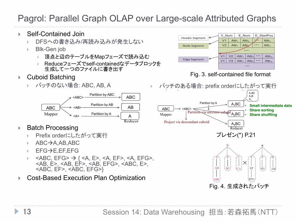
13

}  Self-Contained Join }  DFSへの書き込み/再読み込みが発生しない }  Blk-Gen job

}  頂点と辺のテーブルをMapフェーズで読み込む }  Reduceフェーズでself-containedなデータブロックを

生成して一つのファイルに書き出す }  Cuboid Batching

}  バッチのない場合: ABC, AB, A

}  Batch Processing }  Prefix orderにしたがって実行 }  ABCàA,AB,ABC }  EFGàE,EF,EFG }  <ABC, EFG> à { <A, E>, <A, EF>, <A, EFG>,

<AB, E>, <AB, EF>, <AB, EFG>, <ABC, E>, <ABC, EF>, <ABC, EFG>}

}  Cost-Based Execution Plan Optimization



as a Cubing job, where each cuboid is processed independently.Obviously, calculating the cuboids in V-Agg and E-Agg basedon the original vertex and edge attribute tables is more suitablethan the joined data. Thus, this cubing job can take bothoriginal tables and joined data as input. Recall that each cuboidin the VE-Agg is an aggregate graph as defined in Definition 4.To construct such an aggregate graph, each condensed vertexactually can be calculated while processing the cuboids in V-Agg since they would group the vertices in the same way.Thus, we only need to calculate the weighted edges betweentwo condensed vertices in the aggregate graph based on thejoined data. The algorithm is provided in Alg. 1. This naivealgorithm extracts, shuffles and processes each cuboid’s group-by attributes independently.

However, for large attributed graph, such a naive algorithmis expected to perform poorly for two reasons:

Size of joined data: As one vertex may be associatedwith multiple edges, the join output of the Join-Job can bevery large. Assume that the average degree of each vertex, thesize of vertex attribute table and the size of the edge attributetable are d, |V | and |E| respectively. The size of the output ofthe Join-Job is almost d ∗ |V |+ |E|.

Size of intermediate data: Processing each cuboid inde-pendently may generate a large amount of intermediate data,since each cuboid extracts its own (k,v) pairs which will incurhigh sorting/shuffling overheads.

IV. MRGRAPH-CUBING GRAPH CUBE MATERIALIZATION

In this section, we introduce an efficient Hyper Graph Cubecomputation approach, MRGraph-Cubing to handle large at-tributed graphs in Pagrol. We first introduce the overall processof MRGraph-Cubing: 1) It joins the vertex and attribute tables.For this, we propose a self-contained join to avoid writingand reloading the joined data to/from DFS (section IV-A); 2)It groups cuboids into batches so that the intermediate dataand computation can be shared. Our cuboids batching schemeidentifies the cuboids that can be batched (section IV-B); 3) Itfurther bundles batches into bags so that we can process eachbag in a single MR job (section IV-C); 4) To ensure optimalbundling of batches into bags in (3), we further develop acost-based execution plan optimizer that can generate anexecution plan to minimize the cube computation time (sectionIV-D).

A. Self-Contained Join

To reduce the high overhead incurred by the large joineddata from the first Join-Job, we propose a self-contained jointechnique to postpone the join operation to the map side of thesecond cubing MR job. In so doing, after the join, the data willbe directly used for graph cube computation and do not needto be written/reloaded via DFS. However, a self-contained joinrequires the data in each mapper to contain the edges and theircorresponding vertices. Thus, instead of a Join-Job, we issuea Blk-Gen MR job to reorganize the original data into a seriesof self-contained data files.

In particular, the Blk-Gen job reads both the vertex andedge attribute tables in the map phase. Then it partitions theedges to different reducers according to its two vertex IDs.

!"#$% &"#$% &"'()*(+,-

!. /((*. /((*0 /((*1!0 /((*. /((*0 /((*1

!. !0 /((*. /((*0 /((*%!. !2 /((*. /((*0 /((*%

!"#$"%&'"()"*+

,-$"&'"()"*+

.$("&'"()"*+

Fig. 3. The self-contained file format

Meanwhile, it also partitions the vertex information to thecorresponding reducers whose edges contain the same vertexIDs. Note that each vertex is shuffled to multiple reducers asneeded. In the reduce phase, the Blk-Gen job generates a seriesof self-contained data blocks and outputs each block as onefile whose format is described in Fig. 3. Under this scheme, ineach file, the vertex can be shared by multiple edges insteadof being replicated multiple times.

As MR does not partition the input file if it is not biggerthan one block, each self-contained file will be supplied to onemapper directly to perform a join in the second cubing join.

B. Cuboids Batching

To build a graph cube, computing each cuboid indepen-dently is clearly inefficient. A more efficient solution, whichwe advocate, is to combine cuboids into batches so thatintermediate data and computation can be shared and salvaged.

For the scheme to be effective, we first identify the cuboidsthat can be combined and batched together. Here, we assumethat we materialize the complete cube. Our scheme can beeasily generalized to materialize a partial cube (compute onlyselected cuboids).

Recall that there are three different types of cuboids: V-Agg, E-Agg and VE-Agg. For processing the cuboids in eitherV-Agg or E-Agg, we have developed a solution in [10]. Assuch, we shall give an overview here as our focus in thiswork is on the VE-Agg; interested readers are referred to thepaper for details. The collection V-Agg/E-Agg cuboids canbe batched together under MR if they satisfy the followingcombine criterion:

Criterion 1: Among the multiple V-Agg or E-Agg cuboids,any two of them have the ancestor/descendant relationship andshare the same prefix.

For instance, given 3 V-Agg cuboids C1, C2 and C3, iftheir vertex group-by dimensions are VD1=A, VD2=AB andVD3=ABC respectively, then C1 ≺ C2 ≺ C3 and they sharethe same prefix with each other. In this given example, these 3cuboids can be combined and processed together to facilitatethe MR sorting feature (MR sorts all the intermediate (k,v)pairs according to the key) using the approach we proposedas follows: When the mapper reads each tuple, it emits one(k,v) pair to serve C1,C2 and C3 where VD3 is set as the keyand VD1 is used to partition the intermediate pairs, instead ofthe emitting three pairs. This would guarantee that the tupleswith the same group-by values of C1, C2 and C3 are shuffledto the same reducer, and thus can be processed together. Morecorrectness proof can be found in [10].

500

Fig. 3. self-contained file format

Cuboid Batching

21

<ABC>

<AB>

<A>

<ABC> Partition by ABC

Partition by AB

Partition by A

Partition by A

A1BC A1B A1

ABC

ABC

� Compute 3 cuboids without batching: ABC, AB, A • Large intermediate data • Sorting overhead • Shuffling overhead

• Small intermediate data • Share sorting • Share shuffling

Mapper

Mapper

Reducer

Reducer

A

AB

ABC

A2BC

A1BC

A3BC


Project via descendant cuboid

Partition via ancestor cuboid

� Computing cuboids into batch: according to prefix order

プレゼン(*) P.21

The benefits of this approach are: 1) In the reduce phase,the group-by dimensions are all in sorted order for everycuboid in the batch, since MR would sort the data beforesupplying to the reduce function. This is an efficient wayof cube computation since it obtains sorting for “free” andno other extra sorting is needed for aggregation. 2) All theancestor cuboids do not need to shuffle their own intermediatedata but use their descendant’s. This would significantly reducethe intermediate data size, and thus remove a lot of datasorting/partitioning/shuffling overheads.

In Graph cube computation, we claim that the cuboids inVE-Agg can be batched together under MR if they satisfy thefollowing combine criterion:

Criterion 2: Among the multiple VE-Agg cuboids, any twoof them have the ancestor/descendant relationship. In addition,the V-Dims between any two of the cuboids share the sameprefix, as well as their E-Dims.

Intuitively, to obtain the aggregate graph of each VE-Aggcuboid, the procedure can be divided into two parts: 1) Inpart 1, the vertices with the same V-Dims are grouped intocondensed vertices and each condensed vertex’s weight iscomputed using the vertex aggregate function. 2) In part 2, theedges with the same V-Dims of the two vertices and the sameE-Dims are grouped into condensed edges weighted using theedge aggregate function. As we have mentioned before, thefirst part can be conducted with the V-Agg cuboids since theyshare the same vertex grouping condition. Note that if theaggregate function of V-Agg is the same as the one in the VE-Agg, the result of V-Agg can be directly used for constructingthe VE-Agg. Thus, we focus on introducing the approach ofcalculating the weighted edges here.

As an example, suppose we are given three VE-Aggcuboids C1, C2 and C3, where their vertex group-by dimen-sions are VD1=A, VD2=AB and VD3=ABC and edge group-by dimensions are ED1=E, ED2=EF and ED3=EF respectively,then C1 ≺ C2 ≺ C3 and the V-Dims (as well as the E-Dims)share the same prefix order. In this example, C1 and C2 can beprocessed and combined together with C3 into one batch. Notethat calculating the weighted edges is based on the joined edgeseach of which (e) is a triple-tuple: V-Dims of sV (VD(sV)),V-Dims of tV (VD(tV)) and E-Dims of e (ED(e)).

Under MR, C1, C2 and C3 can be processed in one batch asfollows: When one mapper parses one joined edge e, it emitsone (k,v) pair to serve C1, C2 and C3 where the concatenationof VD3(sV), VD3(tV) and ED3(e) (which is ABCABCEF)as the key. And the concatenation of VD1(sV), VD1(tV) andED1(e) (which is AAE) is used to partition the (k,v) pairs. Thisguarantees that all the edges with the same group-by valuesof C1, C2 and C3 are shuffled to the same reducer, thus theycan be processed together.

Now, we formally define two special cuboids within onebatch.

Definition 6 (Project Cuboid): Given one batch, if allother cuboids are the ancestors of cuboid A, A is defined asthe Project Cuboid, denoted as Pro Cubd. During the cubecomputation, the aggregation dimensions of A are projectedas the key to serve all other cuboids within the batch underMR.

!

" # $

"# #$ $"

"#$

%

!

& '

&' '( (&

&'(

(#

#$

$

$" (&

('

'(

"

"#

"#$

&

&'

&'(

Fig. 4. The generated batches

Definition 7 (Partition Cuboid): Given one batch, ifcuboid A is the ancestor of all other cuboids, A is defined asthe Partition Cuboid, denoted as Par Cubd. During the cubecomputation, the aggregation dimensions of the A are used topartition the key.

For instance, given one batch with three V-Agg cuboids{<A,*>, <AB,*>, <ABC,*>}, <ABC,*> and <A,*>are called the Pro Cubd and Par Cubd respectively. Like-wise, given one batch with three VE-Agg cuboids {<A,E>,<AB,EF>, <ABC,EF>}, <ABC,EF> and <A,E> are calledthe Pro Cubd and Par Cubd respectively.

Basically, the more cuboids we combine into one batch,the less intermediate data will be generated and the morecomputation sharing we can get. Based on the aforementionedprinciples, one cuboid can be batched with all its descendantcuboids satisfying criterion 1 or 2. Therefore, to generatebatches, we first search the cuboids in V-Agg and E-Agg andgenerate the batches within V-Agg and E-Agg according tocriterion 1. For instance, given the lattice in Fig. 2 (d), itgenerates three batches within V-Agg and E-Agg as shownin Fig. 4 using the dotted lines.

For VE-Agg, the batch plan can be generated by combiningthe V-Agg batches with the E-Agg batches through cartesianproduct. Let us still take Fig. 2 (d) as an example. Thefinal execution plan will generate 9 batches whose Pro Cubdsare <ABC,EFG>, <ABC,FG>, <ABC, GE>, <BC,EFG>,<BC,FG>, <BC, GE>, <CA,EFG>, <CA,FG> and <CA,GE>. Each batch consists of multiple cuboids. For instance,the batch <ABC, EFG> includes the 9 cuboids <A,E>,<A,EF>, <A,EFG>, <AB,E>, <AB,EF>, <AB,EFG>,<ABC,E>, <ABC, EF> and <ABC,EFG>.

C. Batch Processing

Since processing V-Agg, E-Agg and VE-Agg are all basedon different input data, we propose to process the batches inthese three different types separately. The MR-based algorithmof processing V-Agg and E-Agg is similar to the cube com-putation in relational database [10]. Thus, we omit it here. Asmentioned in section IV-B, calculating the condensed verticescan be integrated with V-Agg. Therefore, in this section, wemainly focus on how the batches in VE-Agg can be processedto get all the condensed and weighted edges.

Given a computing cluster and a set of batches, there aremultiple plans to process all the batches.

Definition 8 (Execution Plan): Given a set of batchesB={B1, B2, ..., Bx} , the execution plan is a set of MR jobs

501

Fig. 4. 生成されたバッチ

Cuboid Batching

21

<ABC>

<AB>

<A>

<ABC> Partition by ABC

Partition by AB

Partition by A

Partition by A

A1BC A1B A1

ABC

ABC

� Compute 3 cuboids without batching: ABC, AB, A • Large intermediate data • Sorting overhead • Shuffling overhead

• Small intermediate data • Share sorting • Share shuffling

Mapper

Mapper

Reducer

Reducer

A

AB

ABC

A2BC

A1BC

A3BC


Project via descendant cuboid

Partition via ancestor cuboid

� Computing cuboids into batch: according to prefix order

}  バッチのある場合: prefix orderにしたがって実行

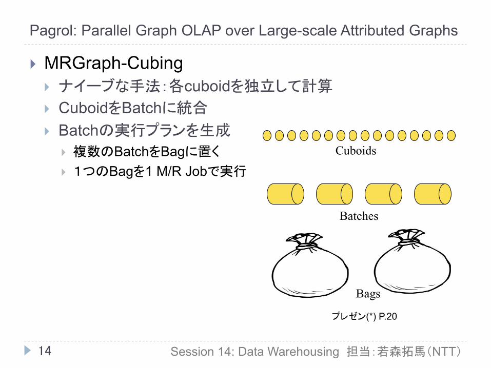
14

}  MRGraph-Cubing }  ナイーブな手法：各cuboidを独立して計算 }  CuboidをBatchに統合 }  Batchの実行プランを生成

}  複数のBatchをBagに置く }  １つのBagを1 M/R Jobで実行



Cube Materialization � Naïve: Calculating each cuboid independently � MRGraph-Cubing approach

Combine the cuboids into batches Generate the batch execution plan ¾ Put different batches into bags ¾ Run each bag using one MR job

Cuboids

20

Batches

Bags

Motivation | Graph Aggregation | Graph Cube Model | Cube Materialization| Experiments プレゼン(*) P.20

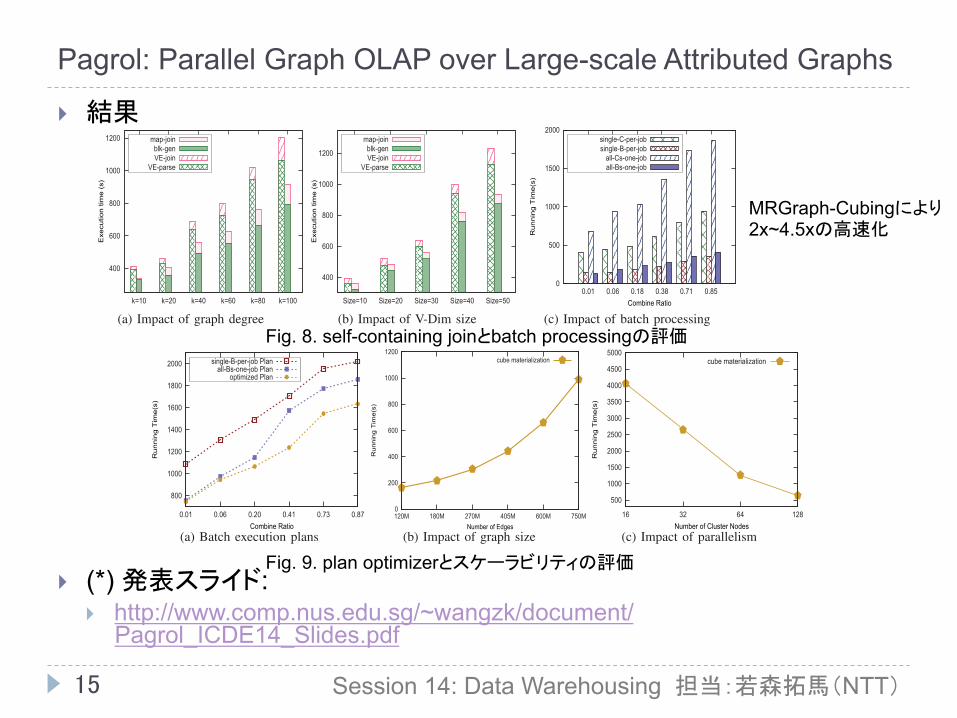
15

}  結果

}  (*) 発表スライド:

}  http://www.comp.nus.edu.sg/~wangzk/document/Pagrol_ICDE14_Slides.pdf



400

600

800

1000

1200

k=10 k=20 k=40 k=60 k=80 k=100

Exe

cutio

n tim

e (s

)

map-joinblk-genVE-join

VE-parse

(a) Impact of graph degree

400

600

800

1000

1200

Size=10 Size=20 Size=30 Size=40 Size=50E

xecu

tion

time

(s)

map-joinblk-genVE-join

VE-parse

(b) Impact of V-Dim size

0

500

1000

1500

2000

0.01 0.06 0.18 0.38 0.71 0.85

Run

ning

Tim

e(s)

Combine Ratio

single-C-per-jobsingle-B-per-job

all-Cs-one-joball-Bs-one-job

(c) Impact of batch processingFig. 8. Evaluation for self-contained join and batch processing

and < {Affiliation, TotalFriends}, ∗ >, we can easily obtainthe top 5 communities which has the largest number of peoplein each category as shown in Fig. 6. We can see that “Teachfor America”, “Texas A&M University” and “New York,NY” have the largest number of people with more than 800friends on Facebook. The result also indicates that “New York”belongs to the top 5 in each category which shows that peopleliving in New York are very active in Facebook.

Next, we investigate how people are connected with eachother between the cities in California: LA (Los Angles), OC(Orange City), SFO (San Francisco) and SV (Silicon Valley).We perform such a query based on the VE-Agg cuboid<Region, Type>. Fig. 7 provides an aggregate graph whichgives us a much simpler and clearer picture of the originalFackbook data. We observe that there are only 4 cross-citycolleague relationships (denoted as C:4 in the figure) betweenSV and SFO. Such a relationship suggests that some compa-nies may be operating in these two cities. By drilling down,we discover that three of the relationships were built amongthe people working in Tellme Inc. which is a big companyoperating in both cities. Another observation is that cross-cityschoolmate relationships (denoted as S:21) appear the mostbetween LA and OC. Our drill-down operation allows us tofigure out that these belong to the Universities in Californialike UCLA. There are still much more interesting information.Due to space constraint, we do not discuss them here. Fromthe results, it is clear that our Hyper Graph Cube model offersan effective mechanism to study and explore the characteristicsof large graphs.

!"#$%"&'

("$

!"$) ("$

%"#*+ !"+,

("-- %"-*-

!"-$("#,

%"#*#

!" #$!!

%"#.

!"+

%"*&

!"-#

#%

!"#,'("#&

&'

%"+-)

%"#+

!"$%"&+!".%"'

!"+

Fig. 7. OLAP query on VE-Agg cuboid <Region, Type>

For the following experiments, we use the synthetic dataset.Each graph contains 3 V-Dims and 3 E-Dims. By default, theaverage size of each V-Dim or E-Dim is 7 bytes. Meanwhile,we choose COUNT(·) as the measure function for both thevertex and edge aggregation. Note that if a graph contains Nedges with degree K, there will be N*2/K vertices in the graph.

B. Self-Contained Join Optimization

In this experiment, we compare the proposed self-containedjoin optimization with the naive approach. For our proposedself-contained join optimization, we have two MR jobs: blk-gen job which reads the vertex and edge attribute tables andgenerates a series of self-contained files, and map-join jobwhich reads the self-contained files, conducts the map sidejoin and ends after the join operation in the map phase. For thenaive approach, we also have two MR jobs: VE-join job whichjoins the vertex with edge attribute tables, and VE-parse jobwhich reads the joined data and ends when it finishes parsingeach joined data in the map phase.

Figure 8 (a) shows the performance comparison on datasetswith 200 million(M) vertices when we vary the graph degreefrom 10 to 100. The results indicate that our optimizationperforms, on average, 30% faster than the naive scheme.

Figure 8 (b) provides the comparison results by using thegraphs with 200M vertices and with degree 40 when we varythe average size of each V-Dim from 10 bytes to 50 bytes. Theresults indicate that our scheme has an average performanceimprovement of 21% over the naive scheme as well.

The insights we gain are: 1) The self-contained join issuperior over the naive join strategy over all the evaluateddatasets; 2) The performance gain is more significant whenthe graph degree is high and the vertex attribute is large.

C. Cuboids Batching Optimization

Next, we study the benefit of our proposed cuboid batchingoptimization. We implement four algorithms. The first two arethe baselines without batching the cuboids: single-C-per-job(computes each cuboid independently in one MR job) andall-Cs-one-job (computes all cuboids in one MR job). Thenext two are with our batching optimization: 1) single-B-per-job (compute each batch in one MR job) and all-Bs-one-job(compute all batches in one MR job).

505

Fig. 8. self-containing joinとbatch processingの評価

800

1000

1200

1400

1600

1800

2000

0.01 0.06 0.20 0.41 0.73 0.87

Run

ning

Tim

e(s)

Combine Ratio

single-B-per-job Planall-Bs-one-job Plan

optimized Plan

(a) Batch execution plans

0

200

400

600

800

1000

1200

120M 180M 270M 405M 600M 750M

Run

ning

Tim

e(s)

Number of Edges

cube materialization

(b) Impact of graph size

500

1000

1500

2000

2500

3000

3500

4000

4500

5000

16 32 64 128

Run

ning

Tim

e(s)

Number of Cluster Nodes

cube materialization

(c) Impact of parallelismFig. 9. Evaluation of the plan optimizer and scalability

Figure 8 (c) provides the comparison results based on thedatasets with 600M edges and with degree 60 when we varythe average combine ratio of the graph. The results indicatethat the algorithms with batching optimization are 2.5X and 4Xfaster than single-C-per-job and all-Cs-one-job respectively.Meanwhile, we observe that the larger the intermediate data(with a bigger combine ratio) are, the higher the performancegain by the batching optimization.

D. Batch Execution Plan Optimization

We next evaluate the proposed batch execution plan opti-mizer. We compare the performance between the plan (opti-mized plan) generated by the optimizer with two basic plans:single-B-per-job and all-Bs-one-job. Fig. 9 (a) shows theresults on the datasets with 600M edges with degree 60 whilevarying the combine ratio from 0.01 to 0.87. The executiontime is the complete graph materialization time including thefirst Blk-Gen job. For the optimized plan approach, the graphinformation is collected by sampling 1% tuples in the memoryin the Blk-Gen job.

The results show that the execution time of the optimizedplan and all-Bs-one-job is much shorter than single-B-per-job when the combine ratio is low. When the combine ratioequals to 0.01, the optimized plan is the same as the all-Bs-one-job. This is reasonable, since when the map outputsize is small, combining all batches in one job is less costly.It also shows that the optimizer can generate much betterplan than the two basic ones when combine ratio increases.From this experiment, we gather the following insights: 1)The in-memory graph information collection for cost modelincurs very low overhead; 2) The optimizer is able to findreasonable execution plan in all cases even with a simplesampling approach.

E. Scalability

Finally, we evaluate the scalability of our MRGraph-Cubing approach from two different angles. The first set ofexperiments studies the scalability of the scheme with respectto the size of the datasets. Fig. 9 (b) shows the executiontime of cube computation on the datasets with degree 60when we vary the number of edges from 120M to 750M. Weobserve that when the dataset is 1.5X bigger, the execution

time becomes almost 1.5X slower. This indicates that thealgorithm scales well in terms of dataset size.

The second set of experiments aims at studying the impactof parallelism. Fig. 9 (c) provides the execution times of cubematerialization on a dataset with 750M vertices with degree60 when we vary the cluster size from 16 to 128 nodes. Theresults indicate that when the computation power is doubled,the execution time almost reduces to half from 16 to 64 nodes.This confirms that the algorithm scales linearly up to 64 nodes.Beyond 64 nodes, the benefit of parallelism decreases a little.This is reasonable since the MR framework setup time mayreduce the benefits of increasing the computation resourceswhen the cube computation time is not long enough.

VI. RELATED WORK

Data Cubes: Data cubes have been widely used as apowerful tool in traditional data warehousing and OLAP [2].Many researches have been devoted to developing efficientcube materialization algorithms under a centralized system ora small number of nodes [15][16] [17] as well as on MR[18] [10] [19]. However, since the traditional data cubes modelignores the graph structure, these existing algorithms cannotbe directly applied for graph cube computation.

Graph Summarization and Simplification: Our workis related to the research that aims to summarize or simplifygraphs. For instance, [20] proposed to simplify a graph bypreserving its skeleton with topological features. As anotherexample, [21] summarized a graph by extracting simple graphcharacteristics like degrees and hot plots. Graph clustering[22] is another proposed method that summarize the graphsbased on different partitioned regions. However, most of thesestudies focused on unlabeled graphs and it is hard to navigatew.r.t the underlying networks without analysis from differentperspectives as well. [23] is the closest work to graph OLAPwhich also summarized attributed graphs. The work introducedSNAP (Summarization by grouping Nodes on Attributes andPairwise relationship) and a less restrictive k-SNAP whichsummarizes the graph to k clusters based on the user inputattributes, relationships and k. The difference between k-SNAPand Pagrol is the roll-up/drill-down manner. In k-SNAP, theseoperations are performed by decreasing/increasing the numberof k which may lead different number of clusters. Differently,these operations in Pagrol are performed along the hieraticaldimensions upon the attributed graphs.

506

Fig. 9. plan optimizerとスケーラビリティの評価

MRGraph-Cubingにより 2x~4.5xの高速化

Technology

ICDE2014 Session 14 Data Warehousing