農業政策の評価のための応用一般均衡モデルの構造

誌名誌名 農村工学研究所技報

ISSNISSN 18823289

著者著者 國光, 洋二

巻/号巻/号 212号

掲載ページ掲載ページ p. 189-209正誤表

発行年月発行年月 2012年3月

農林水産省 農林水産技術会議事務局筑波産学連携支援センターTsukuba Business-Academia Cooperation Support Center, Agriculture, Forestry and Fisheries Research CouncilSecretariat

[ ~I1iJftHR 212 ]

189 ~ 209, 2012

A Dynamic Computable General Equilibrium (CGE) Model for Analysis of Rural Development Policies

Yoji KUNIMITSU*

Contents

189

I Introduction·········· ............ ...... ......... ......... .. ....................................................... .......... .. ........... 189

II Model················ .... ........ ...... ......... ......... .. ....... ...... .................. ...... ............ ...... .......... .. ........... 190

1 Outline of the model . ...... ...... ......... ......... .... ..... ...... .................. ...... ...... ...... ...... ...... ...... ........... 190

2 Production offirm .. ........ ...... ......... .................... .... .................................... ...... ............ ........... 192

3 Consumption demand of household .... ......... ........... .......... ............ ...... ........ ...................... ........... 195

4 Export and import .................................................................................................................. 197

5 Public spending ..................................................................................................................... 198

6 Commodity demand by investment .. .. ....... .. ......... ......... .... ................................... ....................... 199

7 Market clearing conditions and price definitions ... .. .. ......... .... ............ ...... ...... .......................... ........ 200

ill Calibration···· ...... ...... ............. .. ....... .. .. .. .. .................. ............ .......... .. .... ...... ........ ......... . .. .... .... 200

1 Production parameters .... ....... .. ....... ........ ... .... ..... ...... .... ...... .. ...... .... .. ...... ................................ 200

2 Consumption parameters ........ .. ....... .. ...... ... .. ....... .... .. ...... .. .. .. ...... .... .. ........................... ........... 20 I

3 Parameters of export and import·· ................................... ............ ............ ...... ...... .... .. .. .... .... .. ........ 202

4 Parameters of public spending ...................... ......... ........................ ...... .... .. ...... .... .. .......... .. ...... .. 202

N Model closure, Walras' law and recursive dynamics' ......... .. .... ...... ............ .................. .... .. ...... ...... .. ...... 202

V Outputs of the model .................................................................................................................. 203

VI Conclusion' ........ .... .. .. .. .... .. ....... .. ............... ..... .. .. .......................................... ...... ...... ...... ........ 203

Appendix···· ............ ...... ...... ...... ......... ............... ......... ..................... .......... ..................... .. ...... ........ 205

Acknowledgements···· .. .... ...... ............... ......... ...... ....... .. ....... .............. ..................... ............ .............. 208

References .............................................................................................................................. ..... . 208

Summary (in Japanese) ..................................................................................................................... 209

I Introduction

Japanese rural development policies have changed many times during the 21st century. For instance, asset man­

agement measures for prolonging durable years of irrigation and drainage facilities, drastic reduction in agricultural

public investment, and direct payment to farmers for income support have been decided as new policies. In addition to

these policies, the agricultural trade policy may change, because Japan has expressed an intention to participate in the

meeting of the Trans-Pacific Partnership (TPP). These policy measures definitely affect agricultural production, prices

of food and farmers' income. To evaluate policy measures, the degree of impacts must be quantified in view of eco­

nomics.

The influences of changes in the rural development policy are not only confined to the agricultural sector but

spread to various fields, such as other industrial production and employment. These influences are complicated. Fur­

thermore, economies change according to exogenous conditions, such as a rise in the petroleum price, a rise in the im-

* Laboratory of Project Evaluation, Rural Development Planning Division

Received: 13 December 2011

Keywords: Dynamic CGE model, optimization behavior, first order condition, policy evaluation

190

port food price, and a decrease in population of rural areas, which simultaneously affect the real economies along with

policy changes. As a matter of fact, it is difficult for researchers to see exact effects of policy changes by separating

exogenous changes. In order to evaluate the new rural development policy, we have to quantify and designate the exact

effect of policy changes before and after (or with-and-without) the introduction ofa new policy. For this purpose, an

economic model based on the economic theory that can duplicate real situations is important.

Actually, many models have been used for policy evaluation. Among these models, the computable general equi­

librium (CGE) model can deal with all markets related each other and can measure the ripple effects of initial policy

changes. Also, this model is based on the optimization of economic actors subject to a restriction of resources such as

labor and land, so the trade-off effects caused by a policy change can be easily taken into account. Trade-off effects are

realized in the real economies if an increase in resources of a certain sector decreases resource inputs in other sectors.

Therefore, the CGE models are useful and applicable for policy evaluations.

Several previous studies analyzed the impacts of agricultural policy reform with CGE models. Kilkenny (1993)

used an interregional rural-urban CGE model to show the effects of farm subsidies in the USA and reported that cou­

pled farm subsidies were not as effective as decoupled (nonfarm) income transfers for promotion of rural prosperity.

Taylor, Yunez-Nude and Dyer (1999) also examined the effects of the agricultural decoupling policy with a village

based computable general equilibrium (CGE) model. Their results demonstrated that agricultural policies decoupled

from price stimulated staple production in Mexico. Philippidis and Hubbard (2001) and Gohin (2006) also used the

CGE model to show the effects of the EO's common agricultural policy (CAP) including decoupled support payments

and partially decoupled support under cross-compliance. These studies showed that the EO's CAP has a marked effect

on increasing the diversity of production through expansion of domestic food processing sectors, but the effects of this

policy on both arable crop and beef production are negative.

As for the Japanese economies, Saito (2002) analyzed the effects of a farmland consolidation project as agri­

cultural public investment. Kunimitsu (2009) measured the economic effects of irrigation and drainage facilities in

Japanese agriculture. Akune (2010) analyzed the economic linkage in the green tea industry. The CGE model used in

these studies were static models. The dynamic CGE model was used by Son et al. (2006), Shibusawa et al. (2007) and

Ban (2007). They respectively analyzed transportation policies, environmental policies and regional effects of policy

change. The application of the dynamic CGE model is ideally suited for evaluating public capital stocks. For evalua­

tion of the public policy, the common CGE model used in the previous studies needs to be modified in its structure by

introducing policy variables.

The present study develops a dynamic CGE model for policy evaluation and explains the structure of the model in

detail. Features of this model are to introduce special structures for agricultural production and food consumption and

to install a recursive dynamic structure.

Following this section, how to derive the equations in the model is presented based on the optimization behavior

of the economic actors in the next section. The third section explains how parameters used in the model can be cali­

brated from real data. The fourth section shows the model closure, Walras' condition and the recursive dynamic struc­

ture. In the fifth section, we show examples of outputs calculated by this model to show how this model functions. The

final section provides the conclusions.

IT Model

Outline of the model

CGE models are the non-linear simultaneous equations that estimated from actual economic data to duplicate and

simulate how an economy might react to changes in policy, technology or other external factors. The equations are

commonly based on neo-c1assical theory, often assuming optimizing behavior of producers, consumers and govern­

ment.

The equations of the CGE model in this study are based on the course materials of EcoMod (2010) which is the

world's leading research, advisory, and educational not-for-profit network dedicated to promoting advanced modeling

and statistical techniques in economic policy and decision making. The equations with "*,, are the same equations in

these materials.

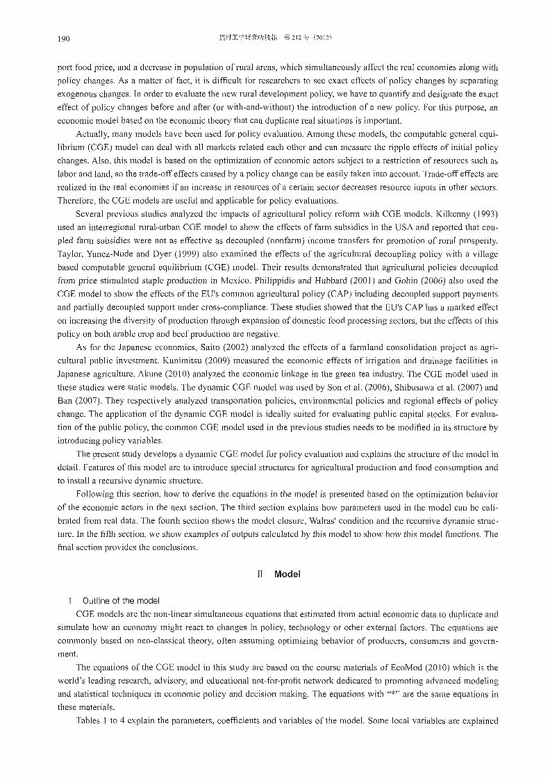
Tables 1 to 4 explain the parameters, coefficients and variables of the model. Some local variables are explained

191

just after equations. Hereafter, the suffix, i,j, and k show the industrial sector and i,j and k =1,2, . . ,n.

Table 1 Parameters for which values are established based on empirical studies

Parameters Explanation

<D Initial value of Frisch parameter in nested-LES (Linear Expenditure System) utility function

I) Initial income elasticities of demand for commodity (sec)

a H Elasticity of substitution between food consumption and other consumptions

a F2i Initial elasticity of substitution between farmland and capital-labor bundle in the CES (Constant Elasticity of Substitution) function (second nest)

a F3 i Initial elasticity of substitution between capital and labor in the CES function (third nest)

a Ai Initial substitution elasticities of the Armington function

a T; Initial elasticities of transformation in the CET (Constant Elasticity of Transformation) function

Table 2 Parameters for which values are estimated by the calibration

Parameters Explanation

II1pS

aHF

aHLESi

alGi

aCGT

aCGi

aFli

aF2i

aF3i

aAi

aT;

Household's marginal propensity to save

Budget shares of CES household utility function in food consumption (CES-function)

Power in the nested household utility function (LES-function)

Subsistence in the household consumption quantities (LES-function)

Cobb-Douglas power of each commodity in the bank's utility function

Cobb-Douglas power of each commodity in the government investment function

Cobb-Douglas power of the public consumption in the government budget

Cobb-Douglas power of each commodity in government utility function

Technical coefficients for intermediate inputs (first nest of production function)

CES distribution parameter for farmland in the firms production function (second nest of production function)

CES distribution parameter for capital in the firms production function (third nest of production function)

CES distribution parameter of commodity in the Armington import function

CET distribution parameter of commodity in the combination of domestic output and export output

Efficiency parameter for capital-labor-farmland bundle in the firm's production function (first nest)

Efficiency parameter in the firm's production function (second nest)

Efficiency parameter in the firm's production function (third nest)

Efficiency parameter of Armington function of commodity (sec)

Shift parameter in the CET function offirm (sec)

Table 3 Coefficients for which values are estimated by the social accounting matrix (SAM) data

Coefficients Explanation

ty

tki

tli

tmi

lv/

d,

Tax rate on income

Tax rate on consumer commodities

Tax rate on capital use

Tax rate on labor use

Tariff rate on imports

Tax rate on value added production including gasoline tax

Depreciation rate for the finns capital stock

rate

192

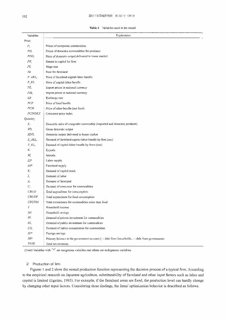
Table 4 Variables used in the model

Variables Explanation

Price

PD;

PDD;

PK;

PL

PA

P_AKL;

P KL

PE;

PM,

ER

PCF

PCM

PCfNDEX

Quantity

X,

XD,

XDD;

X_AKL,

X_KL;

LS*

AS*

K,

L,

CBUD

CBUDF

CBUDM

Y

SH

IP;

fG;

CG,

SF*

SB*

TAXR

Prices of composite commodities

Prices of domestic commodities for producer

Price of domestic output delivered to home market

Return to capital for firm

Wage rate

Rent for farmland

Price of farmland-capital-labor bundle

Price of capital-labor bundle

Export prices in national currency

Import prices in national currency

Exchange rate

Price of food bundle

Price of other bundle (not food)

Consumer price index

Domestic sales of composite commodity (imported and domestic products)

Gross domestic output

Domestic output delivered to home market

Demand offarmland-capital-labor bundle by firm (sec)

Demand of capital-labor bundle by firms (sec)

Exports

Imports

Labor supply

Farmland supply

Demand of capital stock

Demand of labor

Demand of farmland

Demand of consumer for commodities

Total expenditure for consumption

Total expenditure for food consumption

Total expenditure for commodities other than food

Household income

Household savings

Demand of private investment for commodities

Demand of public investment for commodities

Demand of public consumption for commodities

Foreign savings

Primary balance in the government account (+ : debt from households, - : debt from government)

Total tax revenues

(Note) Variables with "*" are exogenous variables and others are endogenous variables.

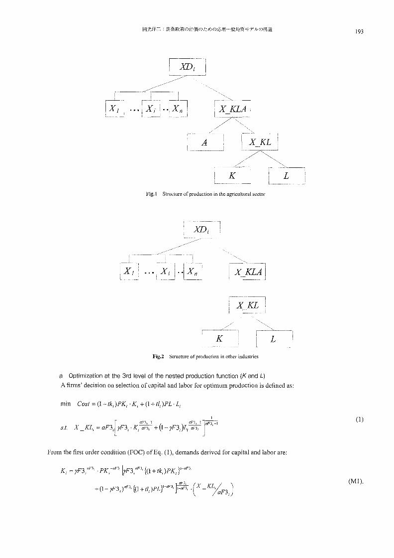
2 Production of firm

Figures 1 and 2 show the nested production function representing the decision process of a typical firm. According

to the empirical research on Japanese agriculture, substitutability of farmland and other input factors such as labor and

capital is limited (Egaitsu, 1985). For example, if the farmland areas are fixed, the production level can hardly change

by changing other input factors. Considering these findings, the firms' optimization behavior is described as follows.

193

Fig.} Structure of production in the agricultural sector

Fig.2 Structure of production in other industries

a Optimization at the 3rd level of the nested production function (K and L)

A firms' decision on selection of capital and labor for optimum production is defined as:

min Cost = (l+tki)PKi ·Ki +(l+tli)PL·Li

(1)

From the first order condition (FOC) ofEq. (1), demands derived for capital and labor are:

Ki = yF3 i oF3, . P Ki -oF3, ~F3 i oF3, {(l + tkJP K}-oF3,

+ (1- rF3i)oF3, {(1 + tli )PL t oF3, J:;~, . (X _K7aF3i

) (Ml).

Li (1- yF3 i) aP3, . P r aP3, ~F3 i 01'3, {(l + tki )P Ki t aF3,

(M2).

Equations that have "M" in front of the number are used in the eGE model, and others are formulae for stages on the

way.

The supply function derived from the zero profit condition is:

b Optimization at the 2nd level of the nested production function (A and KL-bundle)

Firms' decision on the selection of farmland and other input bundles are defined as:

I

s.t. X _ AKLi = aF2i[YF2i . Ai aI;~~~1 + (I yF2i)X _ KLi aI;~~1 Y'2, -I

From the FOe of Eq. (2), demands derived for farmland and for the KL bundle are:

Ai = yF2ial<-2, . P A-ali2, ~F2i aP2, . PA I - aP2,

ali

2 ( ) + (1- yF2J oF2, . P _KLI-

al'- 2, }_ali~, . X _AKYaF2i

X KL = (1- F2. )aI'2, . P KL- al'2, l F2a1i2, . PA I - al'2, -, y., -, y.,

The supply function derived from the zero profit condition is:

c Optimization at the 1 st level of the nested production function (Intermediate inputs and AKL-bundle)

We assume the Leontief-type production function is:

XD = min(X AKLi IOIi ..• 10" ... IOniJ ' aFli ' io

li' 'io,,' 'ioni

(M3).

(2).

(M4).

(MS).

(M6).

(3)*,

where 10 is the intermediate input for production. aF Ii and iOki (i, k = 1,' ... ,n) are the constant technical coefficients.

Assuming that the output XD i is produced at minimum cost, so that no waste of inputs occurs and the ratios lOki lOki

are the same for all i, we can rewrite the above equation as:

XD = X AKLi = 101, = ... = lOki = ... = 10", , aFli iol, iOki iOni

(4)*.

This equation represents the familiar input-output relations for a particular firm:

(M7)* and,

lOki = iOki . XDi for i, k = 1," . " n (5)*. The supply function derived from the zero profit condition is:

195

PDi ·XDi = (1 + tvJP _AKLi·X _AKLi + I(Pk 'iOki ·XDJ k

(M8).

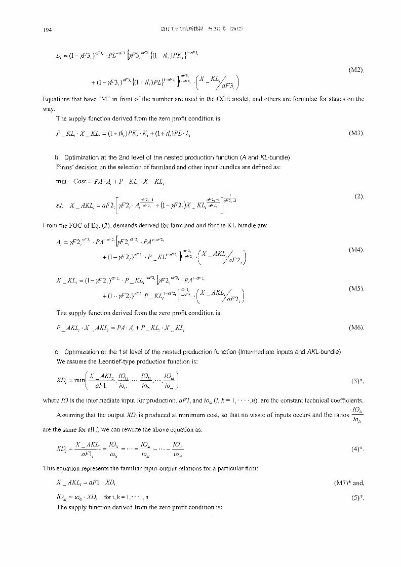
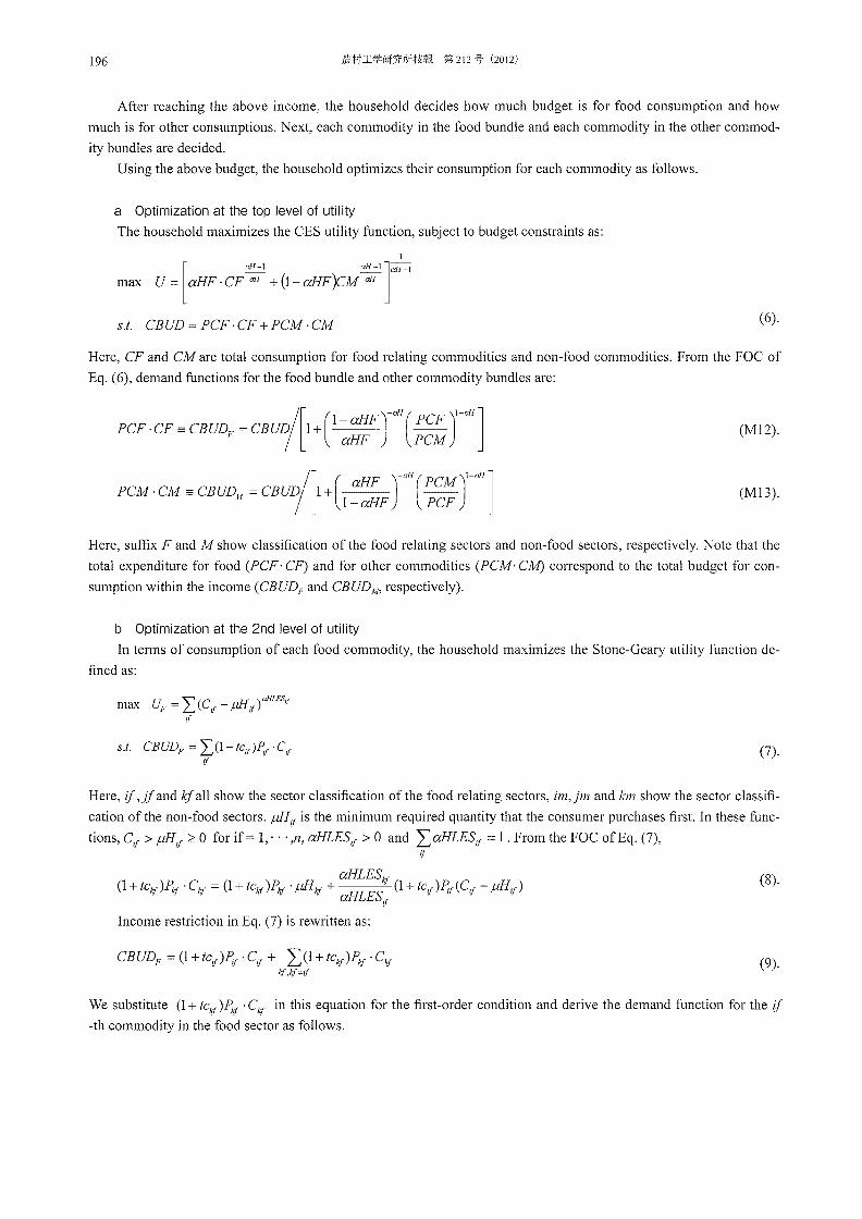
3 Consumption demand of household

Figures 3 and 4 show the structure of household utilities and the decision process for household consumption.

In this model, we assumed that changes in the consumption level of food are quite limited even if the relative price of

U

C n+1

Fig.3 Structure of utilities of a representative household

(Note) CF and CM are total consumption for food relating commodities and non-food commodities.

CBUD

y

KS LS AS

Fig.4 Decision processes of a household

(Note) KS shows nominal capital stocks owned by households and equals total demand for capital stocks in nominal value represented by PK; . K;.

food decreases than other manufacturing products. Also, the basic consumption level exists in consumption behavior

as defined by the Stone-Geary utility function (Neary; 1997, Sadoulet and de Janvry; 1995). The concrete equations for

consumer behavior are derived as follows.

Household income comes from capital revenue, labor income and asset income from land.

(Income definition)

y = "'V P K . K + PL· LS + PA . AS L...., I I

Consumer saves a fraction (mps) of his/her income, so his/her nominal savings are:

SH = mps(l- ty)Y

Consequently, total budget for consumption is:

CBUD = (1 ty)Y - SH

(M9).

(MI0)*.

(Mll)*.

196

After reaching the above income, the household decides how much budget is for food consumption and how

much is for other consumptions. Next, each commodity in the food bundle and each commodity in the other commod­

ity bundles are decided.

Using the above budget, the household optimizes their consumption for each commodity as follows.

a Optimization at the top level of utility

The household maximizes the CES utility function, subject to budget constraints as:

1

max U = aHF· CF df + (1- aHF)cM df [

aff-l aff-ljaff_l

S.t. CBUD=PCF·CF+PCM·CM (6).

Here, CF and CM are total consumption for food relating commodities and non-food commodities. From the FOC of

Eq. (6), demand functions for the food bundle and other commodity bundles are:

PCF· CF = CBUDF = CBUD/[I + C ~:FJaff (;~~ raff

] (MI2).

PCM .CM = CBUD = CBUD/[I+( aHF )-aff(PCM)I-aff] M 7 l-aHF PCF

(M13).

Here, suffix F and M show classification of the food relating sectors and non-food sectors, respectively. Note that the

total expenditure for food (PCF' CF) and for other commodities (PCM' CM) correspond to the total budget for con­

sumption within the income (CBUDF and CBUD/,b respectively).

b Optimization at the 2nd level of utility

In terms of consumption of each food commodity, the household maximizes the Stone-Geary utility function de­

fined as:

max UF = L (Cif - f.iH if tllLES'i

if

S.t. CBUDF = L(l+ tCif)Pif ,Cif if

(7).

Here, if,jjand kjall show the sector classification of the food relating sectors, im,jm and km show the sector classifi­

cation of the non-food sectors. j.iH if is the minimum required quantity that the consumer purchases first. In these func­

tions, Cif > j.iHif ~ 0 for if= 1," . ,11, aHLESif > 0 and ""'LaHLESif = 1. From the FOC ofEq. (7), if

aHLES"f (I + tC"f )P"f' Ckf = (1 + tC"f )P"f' J.lHkf + (I + tCif )J;f(Cif - j.iHif)

aHLESif

Income restriction in Eq. (7) is rewritten as:

CBUDF = (l+tcif)J;f ,Cif + ""'L(1+tChf )Pkf ,Ckf kf,hf¢if

(8).

(9).

We substitute (1 + tCkf )Pkf . Chf in this equation for the first-order condition and derive the demand function for the if

-th commodity in the food sector as follows.

197

(10).

(1 + tClf )Plf . C If = (1 + tClf )Plf . JLl! If

+ aHLESlf [ CBUDF - (1 + tClf )Plf . Clf - ~(l + tClf )Plf . flH If ] (11).

(1 + tClf )Plf . Clf = (1 + tClf )Plf . JLl! If + aHLESlf[CBUDF - 2)1 + tCsf )Psf . JLl!Sf] sf='<tsf

(M14).

As for commodities other than food, a household similarly maximizes the Stone-Geary utility function as follows.

U - ~(C ,,1'4 )aHLES,m max Ai - ~ im - fU.1 im

im

s.t. CBUDM = I(l+tcjnJP;m ,Cjm (12). im

From the FOC ofEq. (12), we derive the demand function for the im-th commodity as:

(l+tCjm)P;m ,Cjm = (1 + tC;m)P;m ·JLl!;m + aHLES;m[CBUDM - I(l+tcsn')Psm .JLl!smJ sm='r/sm

(MIS).

Demand functions shown by Eqs. (MI4) and (MIS) are a linear expenditure system (LES) for the consumption func­

tion.

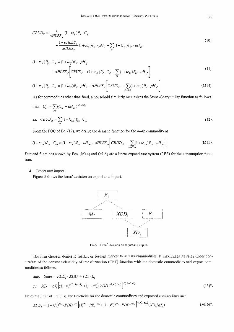
4 Export and import

Figure S shows the firms' decision on export and import.

Fig.5 Firms' decision on export and import.

The firm chooses domestic market or foreign market to sell its commodities. It maximizes its sales under con­

straints of the constant elasticity of transformation (CET) function with the domestic commodities and export com­

modities as follows.

max Sales = PDD; . XDD; + PE; . Ej

t XD. = T [ rr. E(O'T,-I)/oT, + (1- r) XDD(O'T,-I)/O'T, r I(O'T,-I) s. . I a I yl; I r I I (13)* .

From the FOC ofEq. (13), the functions for the domestic commodities and exported commodities are:

XDDj = (1- yT;)oT, . PDDj-oT, ~T;oT, . PE,I-oT, + (1- yT;)"T, . PDD}-oT, jl;/(I-oT,) (XDj / aT;) (M16)*.

198

and

E = Tiff,. PE-u7; [ T U7; • PEI -a7; (1- T)u7; . PDDI-aT, r;/(I-ifl;)(XD/ r) ,'1, ,'1, ,+ '1" , a, (MI7)*.

The supply function derived from the zero profit condition is: PDj . XDj = PEj . Ej + PDDj . XDDj (MI8)*.

The firm produces a composite commodity supplied to the domestic market by using the domestic and imported

commodities. According to the Armington assumption, the optimization behavior is described as:

X A[ ·A ·M(a>I,-I)IO:>I, (1- .A)XDD(o;>I,-I)/"'I,P:>I,/(GI,-I) s.t. j a j YfJ j , + yfJj j J

From the FOC ofEq. (14), the import function and the function for domestic commodities are derived as:

M = ~o;l, . PM-",l, [~GI, . PA;fI-al, (1- ~)O:l, . PDDI-a:l, P:1,/(I-O:I,)(X/ A) ,y., ,y., ,+ y., ,J ,a,

and

XDD =(1 ~»"'l, 'PDD-"'I,[~("l, ·PMI-o:1, +(1 , Y. , ,y. , , ~»"'l, . PDDI-a:I, rA,/(I-O:I,)(X/ A)

}(t I I J I a I

The supply function derived from the zero profit condition is:

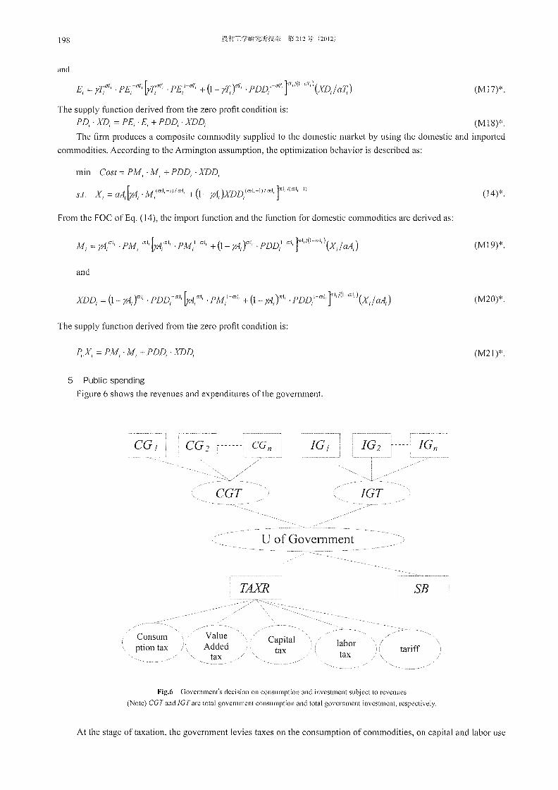
5 Public spending

Figure 6 shows the revenues and expenditures of the government.

CG] CG 2 ------- CGI1

CGT

U of Government

Consum ption tax

Value Added

tax

TAXR

Capital tax

labor tax

IGT

SB

tariff

Fig.6 Government's decision on consumption and investment subject to revenues

(Note) CGTand IGTarc total government consumption and total government investment, respectively>

(14)*.

(M19)*.

(M20)*.

(M21)*.

At the stage of taxation, the government levies taxes on the consumption of commodities, on capital and labor use

199

of firms and on the income of the household. In addition the government obtains revenue from tariffs. Consequently,

the government tax revenues are:

TAXR= 2:0::; ·te; ·C; + tv; .p _AKL;·X _AKL; +tk; ·PK; ·K;

+tl·PL·L +tm ·PWMo; .ER.M)+ty.y I I I I I

Here, PWMo is the initial world price of import commodities.

(M22).

For expenditure part, we assumed that the govemment decides the share of public consumption and public invest­

ment according to public opinions expressed by the national election. In other words, due to political reasons, the share

of expenditures on public consumption and public investment is fixed at the constant ratio against revenue. Total rev­

enue is defined as:

TAXR + SB· PCINDEX

Expenditures of public consumption and public investment are:

PCGT . CGT == aCGT(T AXR + SB . PCINDEX)

PIGT ·IGT == (1- aCGT)(TAXR + SB· PCINDEX)

(15),

(16),

(17).

Here, CGT and IGT are total govemment consumption and total govemment investment, respectively. Total govem­

ment revenue denotes nominal values, but savings from the primary balance in the national account, SB, are defined as

the real value. By definition, when the primary balance is in the red, SB becomes negative indicating the govemment

savings are negative, and vice versa.

After deciding the expenditures, we assumed the efficient behavior of the government. That is, the government

optimizes each expenditure by maximizing the Cobb-Douglas utility function subject to each budget for total public

consumption and total public investment. Optimization decision of the govemment is defined as:

S.t. PIGT ·IGT = 2:1; ·IG; (18),

and

max U IT CG; aCG,

(19).

Here, 2: alG; = 1 and 2: aCG; == 1 . From the FOC of Eqs. (18) and (19) and former Eqs. (16) and (17), the demand

for each commodity in public investment and public consumption can be defined as:

IG; == alG; . p;-l . (1- aCGT)(TAXR + SB· PCINDEX) (M23).

CG; == aCG; . p;-l . aCGT(TAXR + SB· PCINDEX) (M24).

6 Commodity demand by investment

Under macroeconomic restrictions, total savings is always equal total investment. In our model, total savings con­

sist of total household savings, SH, the savings from the primary balance in the national account, SB, and trade surplus

in the foreign account, SF. Note that SB is the real value. The agent "Bank" maximizes the utility defined by a Cobb­

Douglas function subject to the Investment-Savings balance as:

200

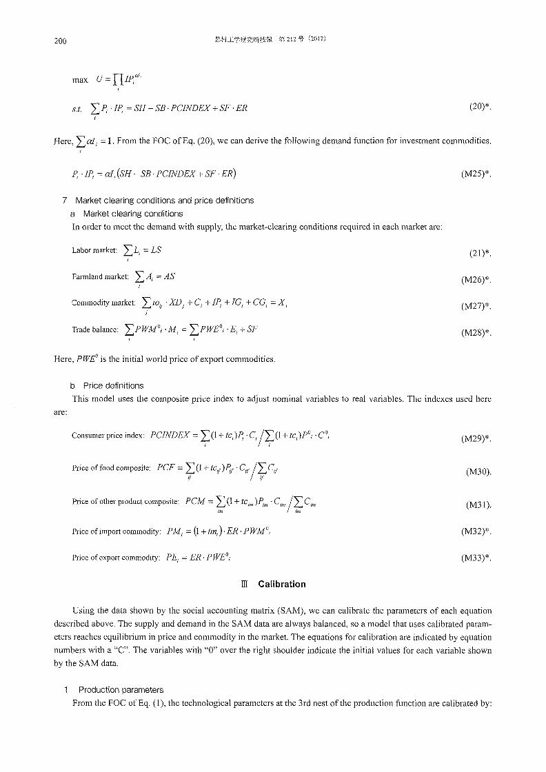
max U = IT IP; ai,

s.t. Ip;· IP; = SH - SB· PCINDEX + SF· ER (20)*.

Here, Ial j = 1. From the FOC ofEq. (20), we can derive the following demand function for investment commodities.

P; ·Ip; = al; (SH - SB· PCINDEX + SF· ER)

7 Market clearing conditions and price definitions

a Market clearing conditions

In order to meet the demand with supply, the market-clearing conditions required in each market are:

Labor market: IL; = LS

Farmland market: I A; = AS

Here, PWEo is the initial world price of export commodities.

b Price definitions

(M25)*.

(21)* .

(M26)*.

(M27)*.

(M28)*.

This model uses the composite price index to adjust nominal variables to real variables. The indexes used here

are:

Consumer price index: PCINDEX = I(1 + tcJ?; ,Cj/IO + tcj)po;. Co; I I

(M29)*.

Price offood composite: PCF = 2)1 + tClf )Plf . clf/I Clf If If

(M30).

Price of other product composite: PCM = I (1 + tC jlll )P;1lI . C;1lI II C;1lI 1111 1111

(M3l).

Price of import commodity: PMj = (1 + tm} ER· PWMo; (M32)*.

Price of export commodity: P E; = ER· P WED; (M33)*.

III Calibration

Using the data shown by the social accounting matrix (SAM), we can calibrate the parameters of each equation

described above. The supply and demand in the SAM data are always balanced, so a model that uses calibrated param­

eters reaches equilibrium in price and commodity in the market. The equations for calibration are indicated by equation

numbers with a "C". The variables with "0" over the right shoulder indicate the initial values for each variable shown

by the SAM data.

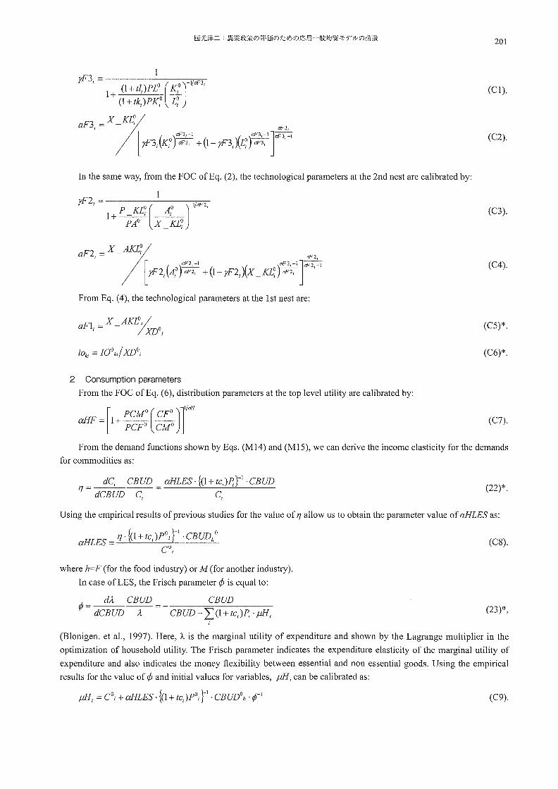
Production parameters

From the FOC ofEq. (1), the technological parameters at the 3rd nest of the production function are calibrated by:

201

(Cl).

(C2).

In the same way, from the FOC ofEq. (2), the technological parameters at the 2nd nest are calibrated by:

(C3).

(C4).

From Eq. (4), the technological parameters at the 1st nest are:

Fl. = X _AKLoi / a I /XDOi (CS)*.

(C6)*.

2 Consumption parameters

From the FOC ofEq. (6), distribution parameters at the top level utility are calibrated by:

allF = 1+ PCM CF [

° ( ° )]l/af{ PCFo CMo

(C7).

From the demand functions shown by Eqs. (M14) and (MIS), we can derive the income elasticity for the demands

for commodities as:

CBUD allLES . {(l + tcJf; }-I . CBUD '7 = -dC-B-U'-D---C-

i - C

i

(22)*.

Using the empirical results of previous studies for the value of 11 allow us to obtain the parameter value of aRLES as:

f ° }-1 ° aHLES = '7 . \(1 + tci)P i . CBUDh

COi (C8).

where h=F (for the food industry) or M (for another industry).

In case ofLES, the Frisch parameter ¢ is equal to:

¢= dA. CBUD dCBUD A.

CBUD (23)*,

(Blonigen, et aI., 1997). Here, Ie is the marginal utility of expenditure and shown by the Lagrange multiplier in the

optimization of household utility. The Frisch parameter indicates the expenditure elasticity of the marginal utility of

expenditure and also indicates the money flexibility between essential and non essential goods. Using the empirical

results for the value of ¢ and initial values for variables, J!lfi can be calibrated as:

° f 0 }-I 0-1 J!lfi = C i + allLES· \(1 + tci)P i . CBUD h • ¢ (C9).

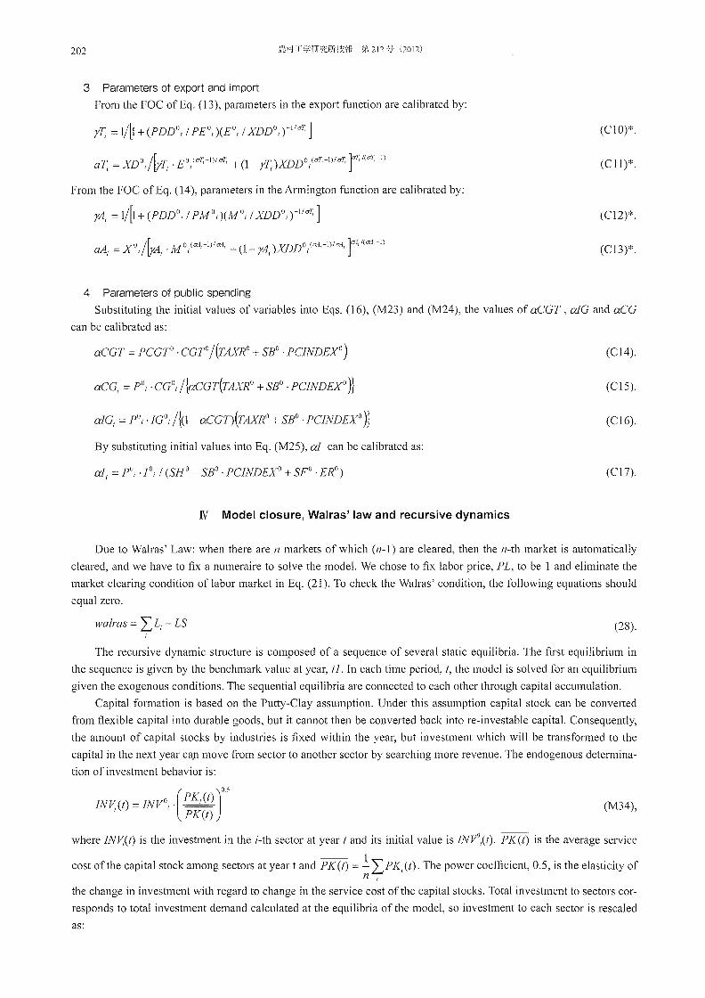
3 Parameters of export and import

From the FOC ofEq. (13), parameters in the export function are calibrated by:

T =XDO/[T .£0(<77;-1)1<77; +(1- T)XDDO(dI;-I)ldI;lrT,I(<77;-I) a ; I Y; I Y; I J

From the FOC ofEq. (14), parameters in the Armington function are calibrated by:

rAj = l/~ + (PDDo; / PMo;)(Mo; / XDDo; r lla7;]

A = XO -/[-;4 . MO(<ffl,-I)IO:l, (1 -;4 )XDDO(O:l,-I)IO:-l, "]a-l,l(o:-l,-I) a; I r.; I + r.; I J

4 Parameters of public spending

(ClO)*.

(Cll)*.

(CI2)*.

(C13)*.

Substituting the initial values of variables into Eqs. (16), (M23) and (M24), the values of aCGT, alG and aCG

can be calibrated as:

(CI4).

(CIS).

(CI6).

By substituting initial values into Eq. (M2S), al can be calibrated as:

(CI7).

N Model closure, Walras' law and recursive dynamics

Due to Wah'as' Law: when there are n markets of which (11-1) are cleared, then the n-th market is automatically

cleared, and we have to fix a numeraire to solve the model. We chose to fix labor price, PL, to be I and eliminate the

market clearing condition oflabor market in Eq. (21). To check the Wah'as' condition, the following equations should

equal zero.

walras = IL; LS (28).

The recursive dynamic structure is composed of a sequence of several static equilibria. The first equilibrium in

the sequence is given by the benchmark value at year, fl. In each time period, t, the model is solved for an equilibrium

given the exogenous conditions. The sequential equilibria are connected to each other through capital accumulation.

Capital formation is based on the Putty-Clay assumption. Under this assumption capital stock can be converted

from flexible capital into durable goods, but it cannot then be converted back into re-investable capital. Consequently,

the amount of capital stocks by industries is fixed within the year, but investment which will be transformed to the

capital in the next year cap move from sector to another sector by searching more revenue. The endogenous determina­

tion of investment behavior is:

INV(t) = INVo; . (PK;(t)J°.5 I PK(t)

(M34),

where INV;(t) is the investment in the i-th sector at year t and its initial value is INrJY;(t). PK(t) is the average service

cost of the capital stock among sectors at year t and PK(t) .l IpK;(t). The power coefficient, 0.5, is the elasticity of 11 ;

the change in investment with regard to change in the service cost of the capital stocks. Total investment to sectors cor­

responds to total investment demand calculated at the equilibria of the model, so investment to each sector is rescaled

as:

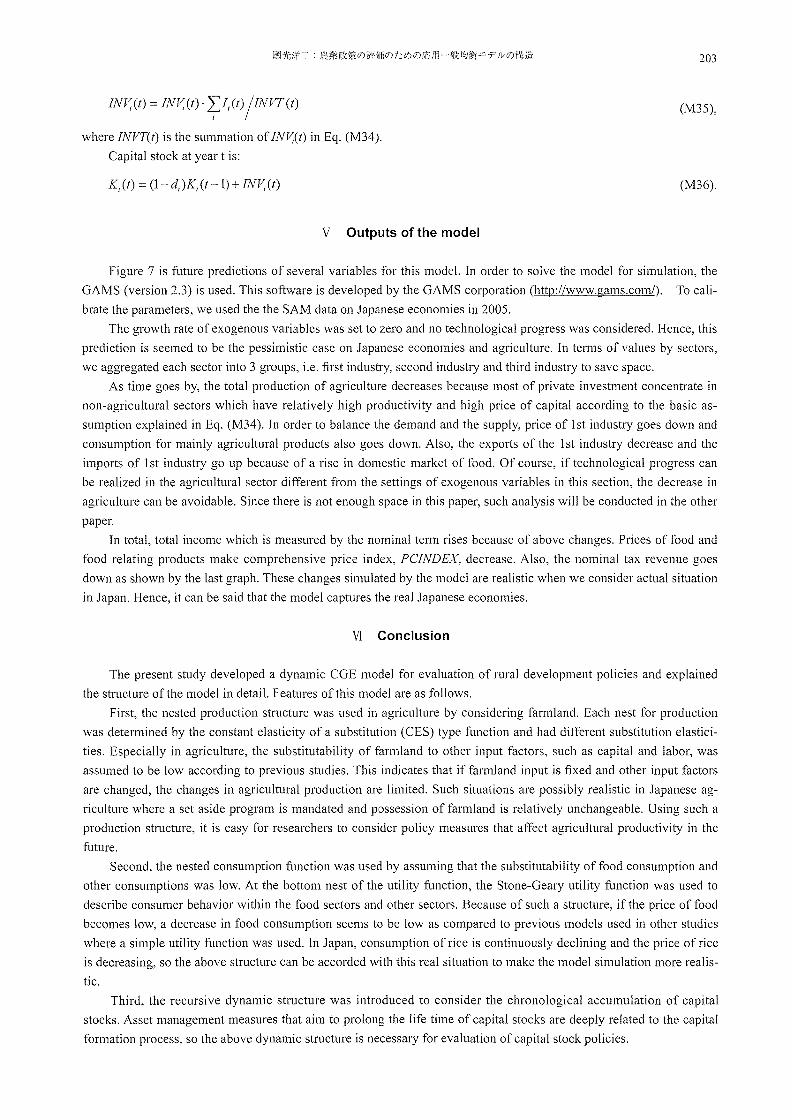
203

IN~(t) = IN~(t)· ~(t) FNVT(t) (M35),

where INVT(t) is the summation of IN~(t) in Eq. (M34).

Capital stock at year tis:

V Outputs of the model

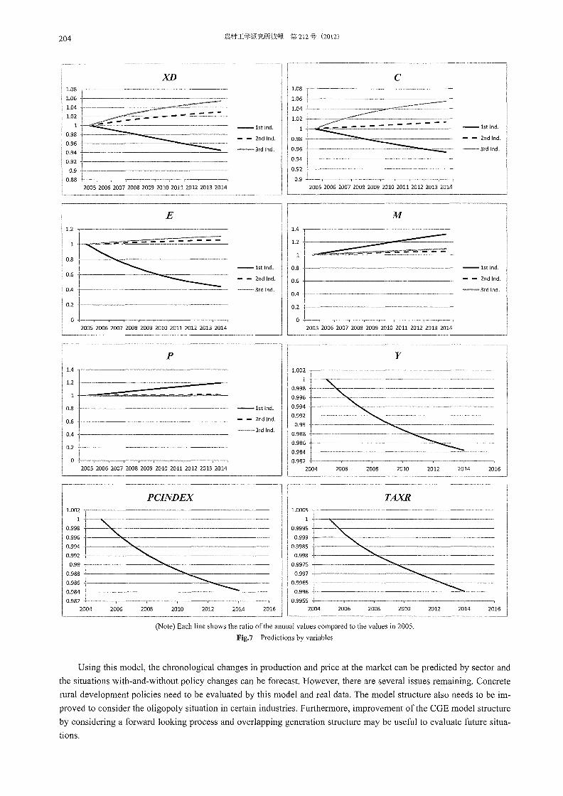
Figure 7 is future predictions of several variables for this model. In order to solve the model for simulation, the

GAMS (version 2.3) is used. This software is developed by the GAMS corporation (http://www.gams.com/). To cali­

brate the parameters, we used the the SAM data on Japanese economies in 2005.

The growth rate of exogenous variables was set to zero and no technological progress was considered. Hence, this

prediction is seemed to be the pessimistic case on Japanese economies and agriculture. In terms of values by sectors,

we aggregated each sector into 3 groups, i.e. first industry, second industry and third industry to save space.

As time goes by, the total production of agriculture decreases because most of private investment concentrate in

non-agricultural sectors which have relatively high productivity and high price of capital according to the basic as­

sumption explained in Eq. (M34). In order to balance the demand and the supply, price of 1st industry goes down and

consumption for mainly agricultural products also goes down. Also, the exports of the 1 st industry decrease and the

imports of 1 st industry go up because of a rise in domestic market of food. Of course, if technological progress can

be realized in the agricultural sector different from the settings of exogenous variables in this section, the decrease in

agriculture can be avoidable. Since there is not enough space in this paper, such analysis will be conducted in the other

paper.

In total, total income which is measured by the nominal term rises because of above changes. Prices of food and

food relating products make comprehensive price index, PCINDEX, decrease. Also, the nominal tax revenue goes

down as shown by the last graph. These changes simulated by the model are realistic when we consider actual situation

in Japan. Hence, it can be said that the model captures the real Japanese economies.

VI Conclusion

The present study developed a dynamic CGE model for evaluation of rural development policies and explained

the structure of the model in detail. Features of this model are as follows.

First, the nested production structure was used in agriculture by considering farmland. Each nest for production

was determined by the constant elasticity of a substitution (CES) type function and had different substitution elastici­

ties. Especially in agriculture, the substitutability of farmland to other input factors, such as capital and labor, was

assumed to be low according to previous studies. This indicates that if farmland input is fixed and other input factors

are changed, the changes in agricultural production are limited. Such situations are possibly realistic in Japanese ag­

riculture where a set aside program is mandated and possession of farmland is relatively unchangeable. Using such a

production structure, it is easy for researchers to consider policy measures that affect agricultural productivity in the

future.

Second, the nested consumption function was used by assuming that the substitutability of food consumption and

other consumptions was low. At the bottom nest of the utility function, the Stone-Geary utility function was used to

describe consumer behavior within the food sectors and other sectors. Because of such a structure, if the price of food

becomes low, a decrease in food consumption seems to be low as compared to previous models used in other studies

where a simple utility function was used. In Japan, consumption ofrice is continuously declining and the price ofrice

is decreasing, so the above structure can be accorded with this real situation to make the model simulation more realis­

tic.

Third, the recursive dynamic structure was introduced to consider the chronological accumulation of capital

stocks. Asset management measures that aim to prolong the life time of capital stocks are deeply related to the capital

formation process, so the above dynamic structure is necessary for evaluation of capital stock policies.

204

XD 1.08

1.06

1.04

1.02

--1st Ind. 0.98

- - 2nd Ind. 0.96

0.94 --3rdlnd.

0.92

0.9

0.88 2005 2006 2007 2008 2009 2010 2011 2012 2013 2014

E 1.2

0.8

--1st Ind. 0.6

- - 2nd Ind.

0.4 --3rdlnd.

0.2

0 2005 2006 2007 2008 2009 2010 2011 2012 2013 2014

P 1.4 ,-----------------

1.2 [=~=:: __ ===_= __ === 0.8 +----------------- --1st Ind.

0.6 +------------------- - - 2nd Ind.

0.4 -\-------------------3rdlnd.

0.2 1------·-------------

2005 2006 2007 2008 2009 2010 2011 2012 2013 2014

PCINDEX

""-"\..

""" "" ........... .............. -....... ---2006 2008 2010 2012 2014 2016

C 1.08

1.06

1.04

1.02

--1st Ind.

0.98 - - 2nd Ind.

0.96 --3rdlnd.

0.94

0.92

0.9 2005 2006 2007 2008 2009 2010 2011 2012 2013 2014

M 1.4

1.2 ----------== 0.8 --1st Ind.

0.6 - - 2nd Ind.

0.4 --3rdlnd.

0.2

0 2005 2006 2007 2008 2009 2010 2011 2012 2013 2014

1.002

1

, 0.998

0.996

0.994

0.992

0.99

0.988

0.986

0.984

0.982 2004

1.0005

1

0.9995

0.999

0.9985

0.998

0.9975

0.997

0.9965

:

y

"\.. "\..

""" "" "' ............ --........

--......... 2006 2008 2010 2012

TAXR

""-"\..

""" "' .............. ............ .............

.............

(Note) Each line shows the ratio of the annual values compared to the values in 2005.

Fig.7 Predictions by variables

Using this model, the chronological changes in production and price at the market can be predicted by sector and

the situations with-and-without policy changes can be forecast. However, there are several issues remaining. Concrete

rural development policies need to be evaluated by this model and real data. The model structure also needs to be im­

proved to consider the oligopoly situation in certain industries. Furthermore, improvement of the CGE model structure

by considering a forward looking process and overlapping generation structure may be useful to evaluate future situa­

tions.

205

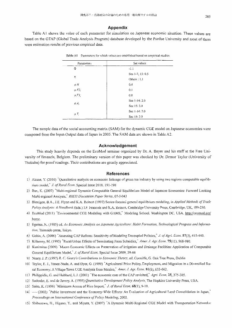
Appendix Table A I shows the value of each parameter for simulation on Japanese economic situation. These values are

based on the GTAP (Global Trade Analysis Program) database developed by the Purdue University and most of them

were estimation results of previous empirical data.

Table Al Parameters for which values are established based on empirical studies

Parameters Set values

(jJ -1.1

Sec 1-7, 15: 0.5 IJ

Others: 1.1

(JH 0.4

(J F2i 0.1

(J F3i 0.8

Sec 1-14: 2.0 (J Ai

Sec 15: 3.0

Sec 1-14: 2.0 (JT,

Sec 15: 3.0

The sample data of the social accounting matrix (SAM) for the dynamic CGE model on Japanese economies were

composed from the Input-Output data of Japan in 2005. The SAM data are shown in Table A2.

Acknowledgement This study heavily depends on the EcoMod seminar organized by Dr. A. Bayer and his staff at the Free Uni­

versity of Brussels, Belgium. The preliminary version of this paper was checked by Dr. Demor Taylor (University of

Tsukuba) for proof readings. Their contributions are greatly appreciated.

References I) Akune, Y. (20 I 0) "Quantitative analysis on economic linkcage of green tea industry by using two regions computable equilib­

rium model," J. of Rural Econ. Special Issue 20 I 0, 191-198

2) Ban, K. (2007) "Multi-regional Dynamic Computable General Equilibrium Model of Japanese Economies: Forward Looking

Multi-regional Analysis," RIETI DiscZlssion Paper Series, 07-J-043

3) Blonigen, B.A., lE. Flynn and K.A. Reinert (J 997) Sector-focused general equilibrium modeling, in Applied Methods of Trade

Policy Analysis: A Handbook (Eds.) J.F. Francois and K.A. Reinert, Cambridge University Press, Cambridge, UK, 189-230.

4) EcoMod (2011) "Environmental CGE Modeling with GAMS," Modeling School, Washington DC, USA, http://ecomod.net/

home.

5) Egaitsu, N. (1985) ed. An Economic Analysis on Japanese Agriculture: Habit Formation, Technological Progress and Informa-

tion, Taimeido press, Tokyo.

6) Gohin, A. (2006) "Assessing CAP Reform: Sensitivity of Modeling Decoupled Policies," J. of Agri. Econ. 57(3), 415-440.

7) Kilkenny, M. (1993) "Rural/Urban Effects of Terminating Farm Subsidies," Ame/: J. Agl: Econ. 75( 11),968-980.

8) Kunimitsu (2009) "Macro Economic Effects on Preservation of Irrigation and Drainage Facilities: Application of Computable

General Equilibrium Model," J. of Rural Econ. Special Issue 2009, 59-66

9) Neary, J. P. (1997) R. C. Gewy's Contributions to Economic TheOlY, ed. Conniffe, G. Oak Tree Press, Dublin

10) Taylor, E. J., Yunez-Nude, A. and Dyer, G. (J 999) "Agricultural Price Policy, Employment, and Migration in a Diversified Ru-

ral Economy: A Village-Town CGE Analysis from Mexico," Amel: J. AgJ: Econ. 81(8), 633-662.

11) Philippidis, G. and Hubbard, LJ. (2001) "The economic cost of the CAP revisited," Agri. Econ. 25, 375-385.

12) Sadoulet, E. and de Janvry, A. (J 995) Quantitative Development Policy AnalYSis, The Hopkins University Press, USA.

13) Saito, K. (1996) "Minimum Access of Rice Import," J. of Rural Econ. 68(1), 9-19.

14) ---- (2002) "Public Investment and the Economy-Wide Effects: An Evaluation of Agricultural Land Consolidation in Japan,"

Proceedings on International Conference of Policy Modeling, 2002.

15) Shibusawa, H., Higano, Y., and Miyata, Y. (2007) "A Dynamic Multi-Regional CGE Model with Transportation Networks:

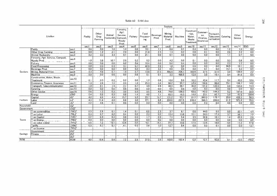
Table A2 SAM data

Forestry,

Other Agri.

Food $ billion Paddy Crop

Animal Service, Fishery Process-Farming

Husbandry Compost, ing

Woody Prod.

sec1 sec2 sec3 sec4 sec5 sec6 Paddv sec1 0.6 0.0 1.0 1.4 0.0 10.1 Other Crop Farming sec2 0.0 1.2 2.1 2.9 0.0 21.6 Animal Husbandry sec3 0.2 0.3 3.3 0.1 0.0 21.1 Forestry, AgrL Service, Compost,

sec4 Woody Prod. 1.8 3.8 10.7 2.9 0.2 0.2 Fishery sec5 0.0 0.0 0.0 0.0 0.8 10.4 Food Processing sec6 0.0 0.0 0.3 3.1 0.7 42.0 Beverage Prod. sec7 0.0 0.0 0.0 0.0 0.2 0.3

Sectors Mining, Material Prod. sec8 2.3 4.9 0.7 1.9 0.7 13.8 Machine sec9 0.0 0.0 0.0 0.0 0.8 0.1 Construction, Water, Waste

sec10 Treatment 0.1 0.3 0.2 0.2 0.0 1.2 Commerce, Finance, Insurance sec11 1.3 2.8 1.5 2.6 1.2 25.3 Transport, Telecommunication sec12 1.0 2.1 1.9 2.1 0.7 9.9 Catering sec13 0.0 0.0 0.0 0.0 0.0 0.0 Other Sevice sec14 0.6 1.3 0.3 3.0 0.3 9.5 Energy ENG 0.4 0.9 0.3 0.8 1.4 4.6 Capital KZ 4.2 6.8 4.9 15.7 5.2 29.7

Factors Labor LZ 4.3 11.4 2.6 6.8 3.0 37.1 Land AZ 2.2 4.6 0.1 0.0 0.0 0.0

Household CZ Government CGZ

T on commodities TRCZ 0.3 0.6 0.1 1.4 0.1 6.8 T on Labor TRLZ 0.3 0.7 0.2 0.4 0.2 2.3 T on Capital TRKZ 0.2 0.4 0.3 0.9 0.3 1.7

Taxes T on Energy TREZ 0.0 0.0 0.0 0.0 0.0 0.0 T on value added TRVZ 0.5 1.2 -0.1 12.6 0.2 -6.1 Tariffs TRMZ 0.3 0.7 0.1 4.1 0.3 5.4 T on Income TRYZ Government fGZ

Savings Private fKZ fSZ

ROW ROW 4.9 10.4 0.4 7.2 2.9 37.5

Sectors

Construct Mining, -ion,

Beverage Material Machine Water,

Prod. Prod. Waste

Treatment

sec7 sec8 sec9 sec10 1.1 0.6 0.1 0.3 2.3 1.3 0.2 0.6 0.0 0.1 0.0 0.0

0.0 4.2 0.0 0.1 0.0 0.0 0.4 0.0 3.9 1.8 0.0 0.0 3.2 0.0 0.0 0.0

12.3 495.6 206.1 169.6 0.1 3.5 498.5 12.6

0.8 16.8 5.9 10.2 5.6 86.2 94.7 54.9 2.6 48.9 39.1 50.9 0.0 0.0 0.0 0.0 4.6 79.6 126.3 63.8 1.1 62.5 16.3 14.8

15.7 131.2 93.7 61.2 8.8 204.0 227.5 248.4 0.0 0.0 0.0 0.0

2.3 3.7 6.1 0.8 0.5 12.4 13.8 15.1 0.9 7.5 5.4 3.5 0.0 0.0 0.0 0.0

14.1 22.7 10.8 17.5 1.0 12.7 9.4 0.0

3.9 169.0 183.4 0.0

Commer-Transport,

ce, Telecomm

Finance, -unication Insurance

sec11 sec12 0.0 0.0 0.1 0.0 0.0 0.0

0.0 0.0 0.0 0.0 0.0 0.0 0.1 0.0

37.5 31.0 3.5 10.1

43.4 11.7 199.6 68.8 131.2 123.9

0.0 0.0 143.3 144.5

23.1 62.7 883.3 175.7 560.3 285.0

0.0 0.0

44.0 9.9 34.0 17.3 50.8 10.1

0.0 0.0 -13.6 16.0

0.0 0.1

12.1 43.8

Catering

sec13 1.2 2.6 1.1

0.3 2.3

30.5 15.1 3.4 0.4

5.4 29.1

8.9 0.0 8.2 5.9

25.0 61.2

0.0

8.0 3.7 1.4 0.0

-4.4 0.0

9.1

Other Energy

Sevice

sec14 ENG 1.0 0.0 2.2 0.0 0.7 0.0

0.8 0.0 1.2 0.0

12.1 0.0 3.3 0.0

139.0 2.2 81.6 0.0

43.5 12.9 156.7 14.8 155.8 13.3

0.0 0.0 197.0 22.0 41.8 I 159.4

439.3 50.3 925.4 25.5

0.0 0.0

22.1 4.4 56.1 1.5 25.3 2.9

0.0 0.0 -1.2 47.8

0.0 13.7

43.5 149.2

H

." ." N o

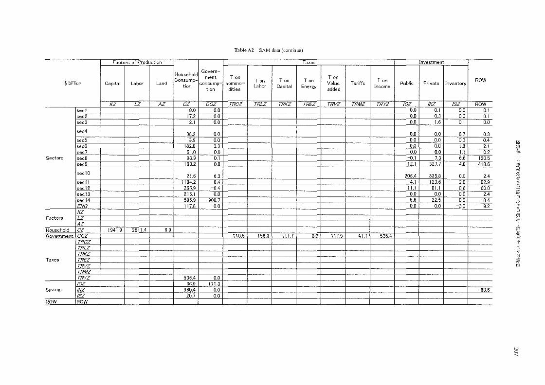
Table A2 SAM data (continue)

Factors of Production Taxes Investment

Household Govern-

Consump- ment Ton Ton Ton Ton

Ton Ton ROW $ billion Capital Labor Land tion

consump- commo- Labor Capital Energy Value Tariffs

Income Public Private Inventory

tion dities added

KZ LZ AZ CZ CGZ TRCZ TRLZ TRKZ TREZ TRVZ TRMZ TRYZ IGZ IKZ ISZ ROW sec1 8.0 0.0 0.0 0.1 0.0 0.1 sec2 17.2 0.0 0.0 0.3 0.0 0.1 sec3 2.1 0.0 0.0 1.6 0.1 0.0

sec4 38.2 0.0 0.0 0.0 6.7 0.3

sec5 3.9 0.0 0.0 0.0 0.0 0.4 sec6 182.8 3.3 0.0 0.0 1.8 2..1 sec7 61.0 0.0 0.0 0.0 1.1 0.2

Sectors sec8 98.9 0.1 0.1 7.3 6.6 130.5 sec9 163.2 0.0 12.1 327.7 4.8 418.6

sec10 21.6 6.3 205.4 335.8 0.0 2.4

sec11 1184.2 0.4 4.1 123.6 2.0 92.9 sec12 265.9 . -0.4 11.1 81.1 0.6 60.0 sec13 216.1 0.0 0.0 0.0 0.0 2.4 sec14 595.9 900.7 5.6 22.5 0.0 18.4 ENG 117.8 0.0 0.0 0.0 -3.0 9.2 KZ

Factors LZ AZ

Household CZ 1941.9 2611.4 6.9 Government CGZ 110.6 158.3 111.7 0.0 117.9 47.7 535.4

TRCZ TRLZ TRKZ

Taxes TREZ TRVZ TRMZ TRYZ 535.4 0.0 IGZ 66.9 171.3

Savings IKZ 960.4 0.0 -60.6 ISZ 20.7 0.0

ROW ROW

208

Equilibrium and Optimality," Studies in Regional Science, 37(2), 375-388.

16) Son, R., Muto, S., Tokunaga, S. and Okiyama, M. (2006) "Quantitative analysis on environmental and energy policy in Chi­

nese automobile industries: Evaluation by the Dynamic Computable General Equilibrium (DCGE) model," Studies in Regional

SCience, 36(1), 113-131.

図光i1'ニ f;21幸政策の評iíIJíのための応用一絞均衡モテソレのtl~j査 209

農業政策の評価のための応用一般均衡モデルの構造

園光洋二

要約

2000年代に入札農家の戸別所得補償やストックマネジメントといった新しい政策が導入される中，これら農業政

策を評備するため、現実の状況を再現でき，経済理論と整合性の高いモデルが必要と考えられる 本研究の目的は，日

本の農業政策の評価のために開発した応用一般均衡モデルの構造を詳織に説明することにある このモデルの特徴は，

第 1に，農業生産において重要である農地を生産要素として考慮するとともに，農地と他の生産要素(労働，資本)の

代替の弾力性が限定的であるという実証研究の結果を考慮したモデル構造としていること，第 2に，人間生活にとって

欠かすことのできない食料消費と他の財・サーピスの沼費の代替性が低いことや，消費において守られるべき最低限の

水準があることを考慮した消費構造としていること，第 3に，資本の蓄積過程を通じた農業生産の変化を評価するため，

逐次動学体系になっていること，等である このモデルを用いることにより，農業政策の影響を価格と生産の両面から，

時系列的に見ることが可誌となる

キーワード:生産要素，代替弾力性，逐次動学体系，資本，労働，農業生産，均衡価格，均衡数量

へ。ーン、ー 訂正箆所

193 6行

式 (M1)

194 l 行

式 (M2)

196 H子

また(6)

196 111子

式 (MI2)

196 12行

まえ(M13)

198 14行

式 (M2])

L

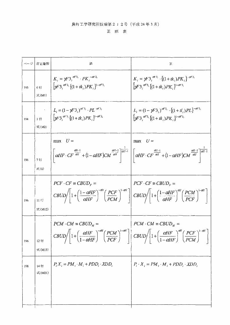
農村工学研究所技報第 212号(平成 24年 3月)

正誤表

誤 工E

Ki = ')F3ロP3r.pK432 ，--1 ----1 Ki = ')F3iaF3，・{(1+ tki )PKi }-aF3，

f.JF3i aF3， {(1 + tk)PK}-aF3， f.JF3; aF3， {(1 + tki )PKi taF3，

Li =(1…')F3JaF3， . praF3， Li = (1-')F3i )aF3， . {(1 + tli )PL }-aF3，

f.JF3iaF3， {(1 + tkJPKi}叩 g f.JF3 i aF3j {(1 +玖)PKi }1-aF3，

max U= max Uご

aHF. CF OH + (1-aHF)cM ----;H [ 出 1 a;;r-1

αHF.CF玄十(l-aHF)cMす[dI171

PCF . CF == CBUDF = PCF. CF == CBUDFご

四句 [1 十C;Ff'(Zr~] αu引I+C:)""(2r~]

PCM・CM==CBUDM ご PCM・CM==CBUDM =

白UD/[I+(品)耐(:2r~] 叫[1+C:;A"(Zr~]

p;.XiコPMi.Mi+PDDi・XDDi p; 'Xi =PMi・Mi十PDDi.XDDi

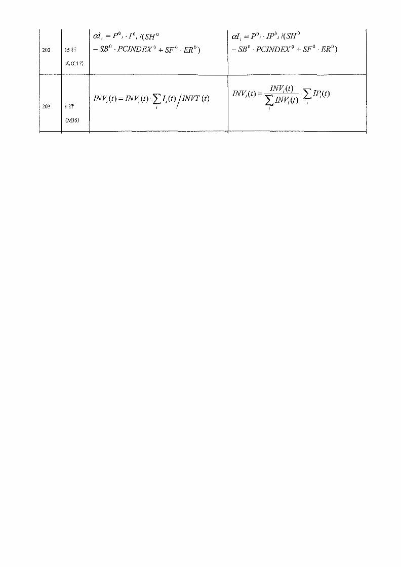
di =P02・IOj/(SHO alj口 pOj'IpOj /(SHD

202 15行 -SBD . PCINDEXO + SpO . ERO) -SBO . PCINDEXO + SpO . ERD)

式(CI7)

IN~ (t) コ I~(t) ・ゃ)~I~(t) 203 Hi

川町仲町(t)平Ii(t円η (t) LIN只(t)~ 2

(M35)