วารสารเศรษฐศาสตรธรรมศาสตร Thammasat Economic Journal ปที่ 23 ฉบับที่ 3 กันยายน 2548 Vol.23, No.3, September 2005

Stock Price Integration in the Malaysian Stock Market

Chan Sok Gee Universiti Tuanku Abdul Rahman

Mohd Zaini Abd Karim Universiti Utara Malaysia

Abstract

There are not many studies in the literature that attempt to analyse market interaction among different sectors within a single stock market. Earlier studies by Grubel and Fadner (1971) highlighted that the interdependence of share price movements is much less pronounced among countries than within a country. Hence, the objective of this paper is to examine the integration relationship within the five major sectors’ price indices listed in the main board of the Malaysian stock market. The results of the study show that there exists a short-run causality relationship between the sectors in the Malaysian stock market for the whole period under study. The daily price movement in the construction sector is found to lead the daily price movement from other sectors for the period before and after financial crisis. This indicates the importance of the construction sector in times of economic boom. However, the trend of causal relationship shifts during the financial crisis in which the finance sector plays a major role in influencing the price movement of other sectors. This may be due to the fact that the financial sector was greatly affected during the financial crisis. The results also show that the causal relationship for both short-run and long run seems to be more obvious in the daily price indices as compared to the weekly price indices. This clearly indicates that the price disturbances in all the sector’s price

124

indices take a relatively shorter time to adjust itself to equilibrium. Thus, the Malaysian stock market is relatively efficient in the adjustment of any short-run and long run disturbances. 1. Introduction

The issue of interdependence between stock markets had been widely studied [Among many others, Grubel and Fardner (1971), Arshanapali and Doukas (1993), Blackman, Holden and Thomas (1994), Chowdury (1994), and Cha and Oh (2000)]. This is because, globalization had reduced the barriers to capital transactions among various countries and increased the linkages between stock markets movement in various countries (Darbar and Deb, 1997). In recent years, foreign investors have expressed an increasing amount of interest in the emerging financial markets of ASEAN and Asian NICs due to their potential and favourable experiences. The interest in this region has led to different studies conducted in ASEAN and Asian Newly Industrialised Countries, especially after the 1997 Asian currency crisis [Among others, Granger, Huang and Yang (2000), Moon (2001) and Daly (2003)]. Most of the studies emphasised on the linkages between the developed and Asian markets, the intra-day and week trading activities in emerging Asian markets and the correlation between risk and return as well as their stability. However, as to our knowledge, there are very few attempts to analyse the market interaction among different sectors within a single stock market. Earlier studies by Grubel and Fadner (1971) highlighted that the interdependence of share price movements is much less pronounced among countries than within a country.

Hence, the objective of this paper is to examine the integration relationship within the five major sectors’ price indices listed in the main board of the Malaysian stock market. This paper provides a detailed analysis of the interdependence of share price movements within sectors in Malaysia. Research on the linkages within the stocks market behaviour in Malaysia is very pertinent in order to better understand many relevant issues pertaining the Malaysian stock market. This is because the Malaysian stock market operated as an emerging market where its

125

function is different in term of cultural, institutional and regulatory circumstances from those in the developed countries.

Fuss (2002) pointed out that regulatory issues that prohibit free market entry and exit restrict capital mobility exist in emerging markets. Thus, the stock markets in emerging markets may operate differently since foreign investors are only allowed to transact investments of a certain kind or to an extent in the domestic market.

In addition, the differences in economic culture and language barriers in emerging market such as Malaysia generate asymmetric information between domestic and foreign investors. The resulting information disadvantages for foreign investors make international investments seem more risky and can only be overcome with additional information costs. Thus, a better understanding of the Malaysian stock market are crucial to provide some insight on the investment opportunities to international investors. Hence, this paper will provide opportunity for better diversification to investors in shifting to higher risk and project return if they were to diversify their overall risk by understanding the linkages between the sectors in the Malaysian stock market. 2. Overview of the Malaysian Stock Market

The equity market provides the avenue for corporations to raise funds by issuing stocks and shares. The secondary market trading in stocks and shares in Malaysia are the Kuala Lumpur Stock Exchange (KLSE) and the Malaysian Exchange of Securities Dealing and Automated Quotation (MESDAQ). The Malayan Stock Exchange was established in March 1960 and public trading of stocks and shares commenced in May 1960 in the clearing house of Bank Negara Malaysia (BNM) (BNM, 1999). In 1968, the Capital Issues Committee (CIC) was established. In 1973, the Malayan Stock Exchange was separated into the Kuala Lumpur Stock Exchange (KLSE) and the Singapore Stock Exchange (SES) due to the termination of currency interchangeability with Singapore and the floating of the Malaysian Ringgit.

126

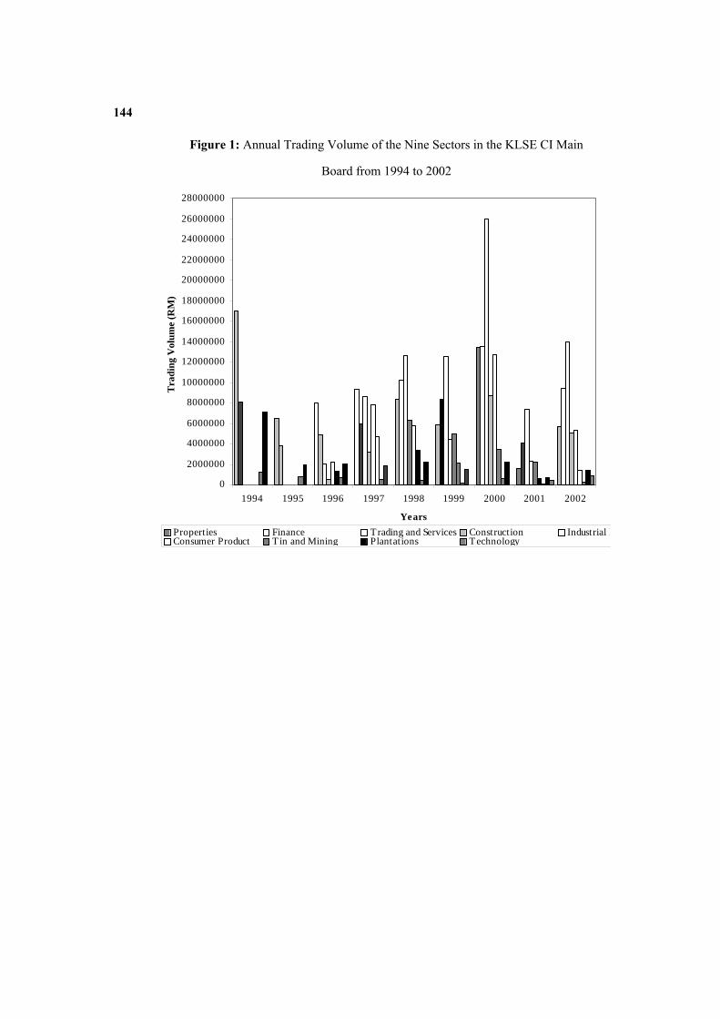
The sectors’ price indices listed in the KLSE is consumer products, industrial products, construction, trading and services, finance, properties, plantation, and mining. Figure 1 shows the trading volume of the nine sectors in the KLSE CI main board from 1994 to 2002. It is clearly indicated that the top five sectors in terms of trading volume over 1994 until 2002 are industrial products, construction, trading and services, finance, and properties.

The funds raised in the Malaysia capital markets had been rising gradually from RM10.3 billion in 1988 to RM33.5 billion in 1997 (BNM, 1999). In addition, the funds raised by the private sector increased from 3% of the Gross Domestic Product (GDP) in 1988 to 12.4% of GDP in 1997. This shows that the capital markets assumed a crucial role in raising funds in Malaysia. The funds raised in capital markets amounted to RM188.4 billion since 1988 until August 1999. The increasing trend in the funds raised in capital markets was mainly due to the strong demand for funds by private sector to finance economic activities. Besides, funds raised in capital markets increased because of the increased in the financing of large-scale industrial investments and infrastructure projects of the corporate sector with a long development period. Moreover, the government’s policy in promoting privatisation also served as one of the factors that caused the increased in funds raised in capital markets. Thus, the capital markets became alternative sources of funds to meet the needs of borrowers. However, the increasing trend in the funds raised was affected in December 1997 as a result of the Asian Financial Crisis. In November 1997, the net funds raised, which amounted to RM3.2 billion declined to RM0.6 billion by December 1997 (BNM, 1999).

3. Data and Methodology

The sample for this study consists of five out of the nine stock indices in the Kuala Lumpur Stock Exchange Composite Index (KLSE) main board. The five major sectors of Kuala Lumpur Stock Exchange Composite Index used in this study are industrial products (IP), construction (CONST), trading and services (TS), finance (FIN), and property (PROP). These

127

sector indices were selected since trading activities in these sectors greatly influenced the movement in the KLSE CI main board.

The data required for the study were acquired from Thomson Datastream. The daily, and weekly closing prices for all the stock indices are employed from January 4 1994 to December 31 2002. The sample is divided into three-time periods based on the study of Moon (2001) on currency crisis and stock market integration. The first period starts from January 4, 1994 to May 30, 1997, which represents the pre-crisis period. The second period starts from June 1, 1997 to February 26, 1999 in which the financial tensions is very high in June 1997 and the effects of financial turmoil became greater in 1998 due to the financial instability in Russia. The financial turmoil was eliminated in March 1999. Thus, the post-crisis period starts from March 1, 1999 until December 31, 2002.

Methodology Unit Root Tests

Unit root test is employed to test the properties of non-stationary in the variables used in this study. Empirical tests for cointegration can only proceed if the series are non-stationary. Unit root tests are important to establish whether the series are integrated with a uniform order of integration (Engle and Granger, 1987). In this analysis, we will test all the series of indices for unit root properties using two commonly used unit root tests, namely Augmented Dickey-Fuller (ADF) test and Phillips-Perron (1988) test. Augmented Dickey-Fuller Tests

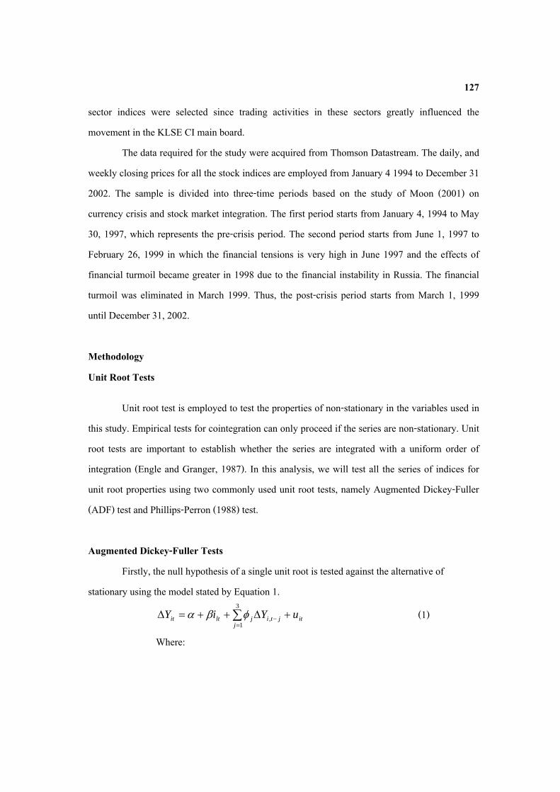
Firstly, the null hypothesis of a single unit root is tested against the alternative of stationary using the model stated by Equation 1.

∑=

− +Δ++=Δ3

1,

jitjtijltit uYiY φβα (1)

Where:

128

1,,, −−−− −=Δ jtijtijti YYY p = number of lagged values of first differences itYΔ , three lags will be included to account for serial correlation in the error term itμ .

The Augmented Dickey-Fuller (ADF) test was conducted by including lagged values of

itYΔ (p≥1) to ensure that the residual itμ is white noise. If the null hypothesis of unit roots is rejected, then the series in level is I (1). Phillips-Perron Unit Root Test

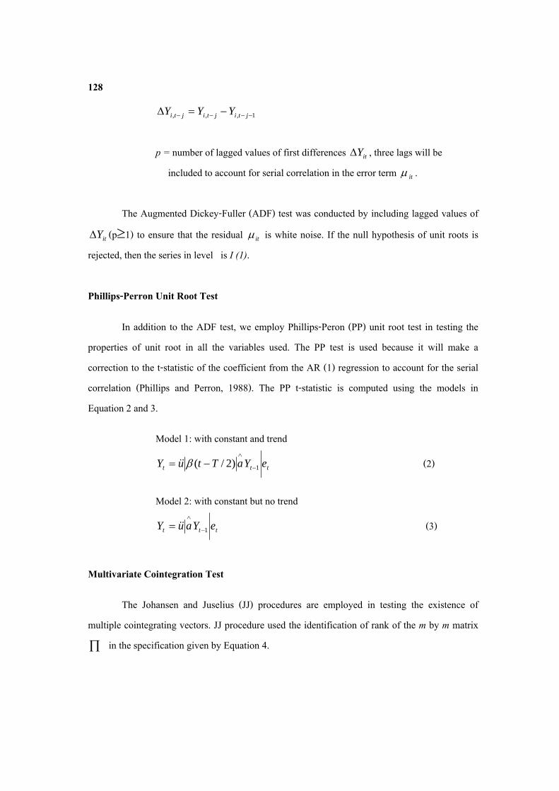
In addition to the ADF test, we employ Phillips-Peron (PP) unit root test in testing the properties of unit root in all the variables used. The PP test is used because it will make a correction to the t-statistic of the coefficient from the AR (1) regression to account for the serial correlation (Phillips and Perron, 1988). The PP t-statistic is computed using the models in Equation 2 and 3.

Model 1: with constant and trend

ttt eYaTtuY 1)2/( −

∧

−= β (2)

Model 2: with constant but no trend

ttt eYauY 1−

∧

= (3)

Multivariate Cointegration Test

The Johansen and Juselius (JJ) procedures are employed in testing the existence of multiple cointegrating vectors. JJ procedure used the identification of rank of the m by m matrix

∏ in the specification given by Equation 4.

129

∑ ∏−

=−− ++Δ+=Δ

1

1

k

itktitt eXXTX δ (4)

Where:

Xt = column vector of the m variables T and ∏ = coefficient matrices

Δ = difference operator k = lag length δ = constant

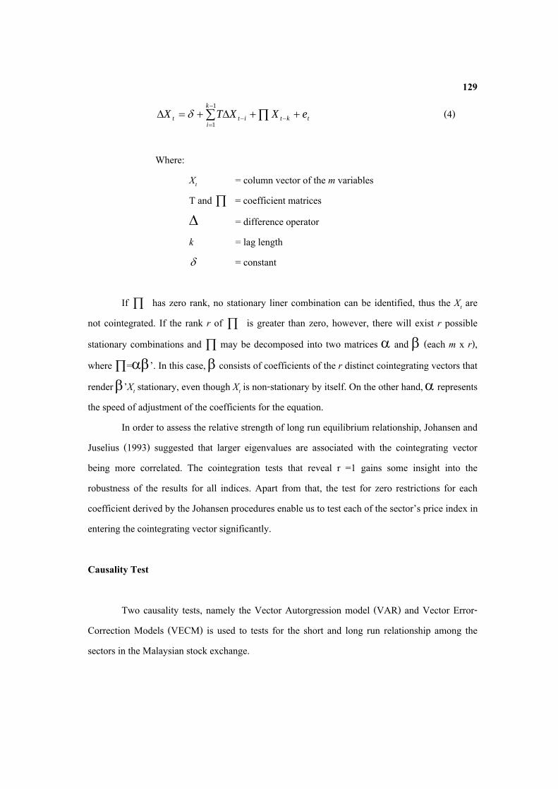
If ∏ has zero rank, no stationary liner combination can be identified, thus the Xt are not cointegrated. If the rank r of ∏ is greater than zero, however, there will exist r possible

stationary combinations and ∏ may be decomposed into two matrices α and β (each m x r),

where ∏=αβ’. In this case, β consists of coefficients of the r distinct cointegrating vectors that

render β’Xt stationary, even though Xt is non-stationary by itself. On the other hand, α represents the speed of adjustment of the coefficients for the equation.

In order to assess the relative strength of long run equilibrium relationship, Johansen and Juselius (1993) suggested that larger eigenvalues are associated with the cointegrating vector being more correlated. The cointegration tests that reveal r =1 gains some insight into the robustness of the results for all indices. Apart from that, the test for zero restrictions for each coefficient derived by the Johansen procedures enable us to test each of the sector’s price index in entering the cointegrating vector significantly. Causality Test

Two causality tests, namely the Vector Autorgression model (VAR) and Vector Error-Correction Models (VECM) is used to tests for the short and long run relationship among the sectors in the Malaysian stock exchange.

130

Vector Autoregression Model (VAR)

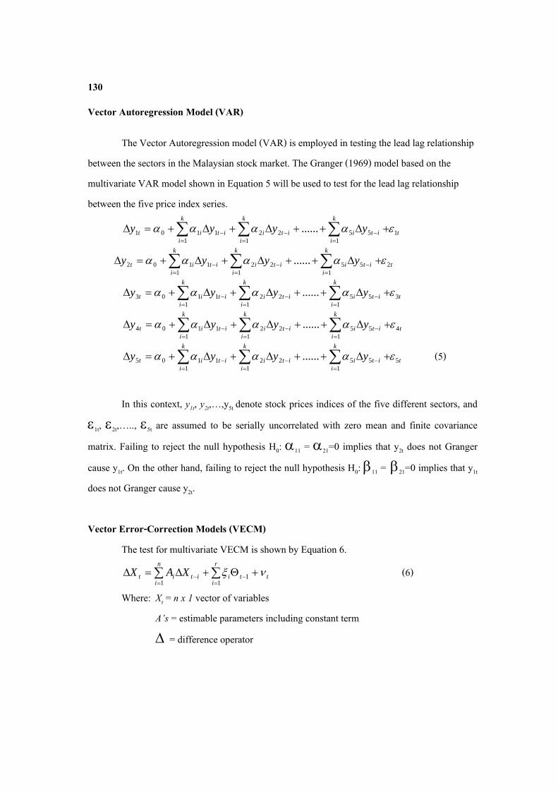
The Vector Autoregression model (VAR) is employed in testing the lead lag relationship between the sectors in the Malaysian stock market. The Granger (1969) model based on the multivariate VAR model shown in Equation 5 will be used to test for the lead lag relationship between the five price index series.

∑ ∑ ∑= = =

−−− +Δ++Δ+Δ+=Δk

i

k

it

k

iitiitiitit yyyy

1 11

155221101 ...... εαααα

∑ ∑ ∑= = =

−−− +Δ++Δ+Δ+=Δk

i

k

it

k

iitiitiitit yyyy

1 12

155221102 ...... εαααα

∑ ∑ ∑= = =

−−− +Δ++Δ+Δ+=Δk

i

k

it

k

iitiitiitit yyyy

1 13

155221103 ...... εαααα

∑ ∑ ∑= = =

−−− +Δ++Δ+Δ+=Δk

i

k

it

k

iitiitiitit yyyy

1 14

155221104 ...... εαααα

∑ ∑ ∑= = =

−−− +Δ++Δ+Δ+=Δk

i

k

it

k

iitiitiitit yyyy

1 15

155221105 ...... εαααα (5)

In this context, y1t, y2t,…,y5t denote stock prices indices of the five different sectors, and

ε1t, ε2t,….., ε5t are assumed to be serially uncorrelated with zero mean and finite covariance

matrix. Failing to reject the null hypothesis H0: α11 = α21=0 implies that y2t does not Granger

cause y1t. On the other hand, failing to reject the null hypothesis H0: β11 = β21=0 implies that y1t does not Granger cause y2t. Vector Error-Correction Models (VECM)

The test for multivariate VECM is shown by Equation 6.

∑ ∑= =

−− +Θ+Δ=Δn

i

r

ittiitit XAX

1 11 νξ (6)

Where: Xt = n x 1 vector of variables A’s = estimable parameters including constant term

Δ = difference operator

131

tξ = vector of impulses that represent the unanticipated movement in Xt Θ = r individual error-correction terms

Equation 3.8 indicated that either ΔX1t ,…, ΔXnt or a combination of any of them may cause by 1−Θ t since it is a function of [X1t-1, …, Xnt-1]. If [X1t-1, …, Xnt-1] shares a common trend, the change in X1t is partly due to X1t moving into alignment with the trend value of X2t ,…,Xnt.

If the variables are cointegrated in the short-term, then the error-correction model indicates that the deviation from long run equilibrium is resulted from the change in dependent variable that force the movement towards the long run equilibrium. If the dependent variable is driven directly by long term equilibrium of I(0) error, then it is said to respond to the feedback. If not, then it is said to respond to short-term shocks to the stochastic environment. The F-test is usually employed in testing the differenced explanatory variables in determining the short-term causal effects, whereas the t-test is used to test the lagged error-correction term in searching for long run relationship between the variables. Finally, the coefficient of lagged error-correction term presents the short-term adjustment coefficients and indicates the proportion by which the long run disequilibrium in the dependent variable is being corrected in each short period. 4. Results and Discussion Unit Root Tests

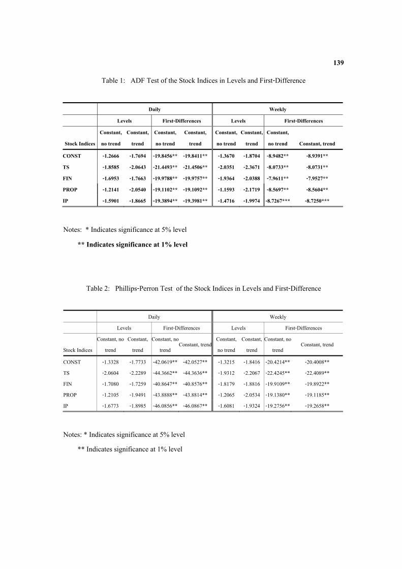
We tested all the series of indices for unit root properties using two commonly used unit root tests, namely Augmented Dickey-Fuller (ADF) test and Phillips-Perron (1988) test. All the stock indices are converted to natural logarithm before the unit root tests are performed. The number of lags employed in this study is determined using Akaike Information criterion (AIC) and Schwarz Criterion (SC). All the unit root tests are conducted using daily and weekly closing prices of stock index.

Table 1 illustrates the results of Augmented Dickey-Fuller (ADF) test for the stock indices in levels and first-differences using daily and weekly data from January 1994 until December 2002. The results show that we cannot reject the null hypothesis of unit root at the 5%

132

and 1% critical value for the five main sector indices in level. Nevertheless, the null hypothesis is rejected at the 5% and 1% critical value when we test on the first-difference of all the series.

The results for Phillips-Perron (1988) test on both levels and first-difference of the series are presented in Table 2. The results show that we cannot reject the null hypothesis of unit root at the 5% and 1% critical value for the series in levels. However, the null hypothesis is rejected at the 5% and 1% critical value when we test on the first-difference of the series implying that the first-difference of these sector’s price indices are stationary. Hence, the sector’s price indices in Malaysia follows I(1) process.

The results obtained from ADF and Phillips-Perron (1988) test for sectors’ price indices support the statement that all differenced logarithmic series, namely the returns and growth series are stationary. Thus, it is possible that the combinations of the stock price series have cointegration property. Hence, we will proceed with the cointegration tests in testing for the cointegration between the stock prices, which are non-stationary in level but stationary in first-difference. Multivariate Cointegration Test

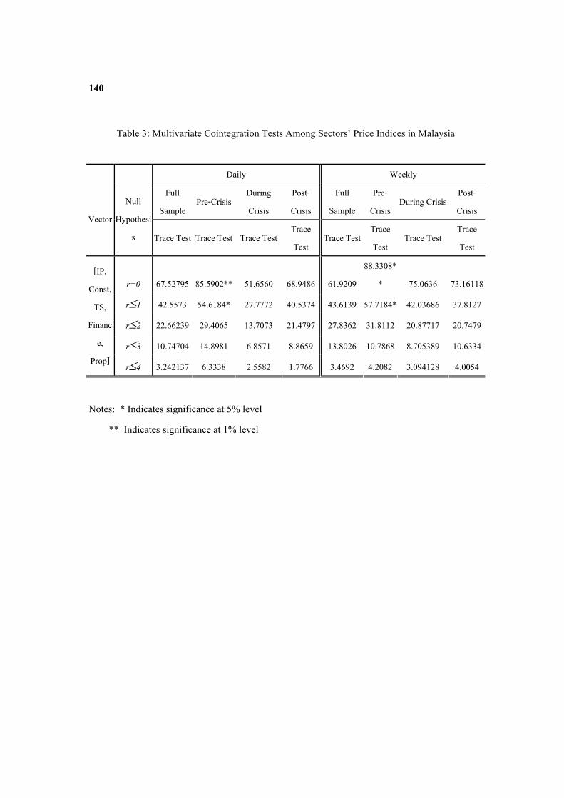
The Johansen and Juselius (JJ) procedures are employed in testing for the existence of multiple cointegrating vectors. This procedure provides more robust results than other cointegration methods when the analysis involves more than two variables (Gonzalo, 1994b). The multivariate cointegration tests are carried out between the sectors’ price indices in the Malaysian stock market. Besides that, the multivariate cointegration tests are also carried out between Malaysian stock market with stock indices from the Philippines, Indonesia, Thailand, Hong Kong, Japan, China and the Unites States in order to gain an insight into the nature of the cointegration relationship between the Malaysian stock market and its major trading partners.

Table 3 illustrates the result of multivariate cointegration test between various sectors’ price indices in Malaysia over the full sample period, pre-crisis period, during crisis period and post crisis period. The results are computed using daily and weekly data in order to gain more

133

understanding of the differences on the changes in stock indices movement between the two data sets.

The results in Table 3 indicate that there are no major differences in the cointegration relationship among the daily and weekly sectors’ price indices in Malaysia. The trace statistics in Table 3 show that the null hypothesis of no cointegrating vector cannot be rejected for both daily and weekly sectors’ price indices when the study is conducted using full sample, during crisis and post-crisis period. The findings also indicated that there exist at most two cointegrating vectors,

i.e. r=0 and r≥1 is rejected at the 1% and 5% significance level respectively before the financial crisis for both daily and weekly sectors’ price indices. Thus, we can conclude that there exists (n-r)= 3 common stochastic trends among this system of sectors’ price indices. Multivariate VAR

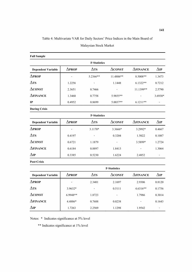
Based on the result obtained from multivariate cointegration test, the multivariate VAR test is conducted in testing for the short-run relationship among all the sector indices in Malaysia, which are not cointegrated. The results for multivariate VAR based on daily sectors’ price indices for full sample, during crisis period, and post-crisis period are presented in Table 4 since the all the sectors are not cointegrated with each other.

The results presented in Table 4 reveal that in the short-run, the daily price movement in the properties sector is led by the daily price changes in the trading and services, the construction and the finance sector for the full sample period. For the period after the financial crisis, the properties sector plays the leading role in leading the daily price movement in the trading and services sector, the construction sector and the finance sector in the short-run. This may be due to the Malaysian government’s policy promoting the development of the properties sector to boost the Malaysia economy after the financial crisis. The banks and financial institutions started to give out more housing loans to their customers after the financial crisis in conjunction with the government’s policies. However, the trend of causal relationships shift during the financial crisis in which the finance sector plays a major role in influencing the price movement of other sector’s

134

price indices. The shift in trend during the financial crisis in which the price index of the finance sector leads the price movement of other sectors are due to the fact that the financial sector is greatly affected during the 1997 crisis. The financial crisis had severely affected the equity market, when the Kuala Lumpur Stock Exchange Composite Index (KLSE CI) fell by 79.3% from 1,271.57 points in February 1997 to 262.70 points on 1 September 1998 (BNM, 1999). The commercial banks and other financial institutions experienced significant turmoil due to the financial crisis. The banking and financial institutions were focused on preserving the quality of their balance sheets and coping with the erosion in their capital instead of generating new loans (BNM, 1999). The pullback effect in loan activities had severely affected the development of the other sectors during the financial crisis.

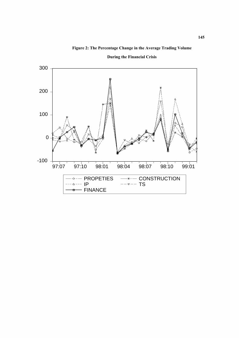
In addition, the leading role of the finance sector during the Asian Financial crisis period might be due to the relatively volatile trading volume in the finance sector. This can be seen from Figure 2 that shows the percentage change in the average trading volume during the financial crisis. From Figure 2, it is clearly illustrated that the finance sector is the most volatile sector in terms of changes in the trading volume especially during the early phase of the financial crisis period that is from June 1997 until March 1998.

Table 5 presents the results of multivariate VAR test on weekly sectors’ price indices in the main board of the Malaysia stock market. From the results in Table 5, the price index of the finance sector has major influence in the market when weekly price indices were employed. Multivariate Error-Correction Model

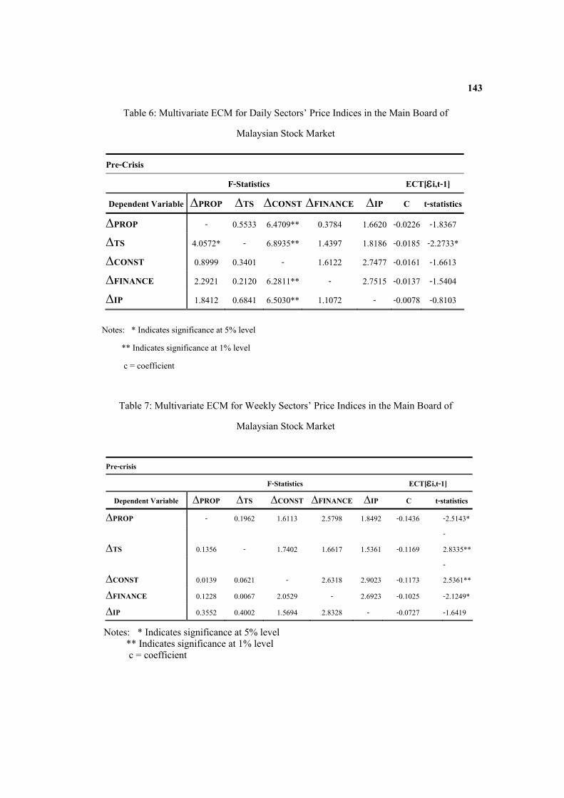
Based on the result obtained from the multivariate cointegration test, the multivariate error-correction (ECM) tests are conducted to test for the long run relationship among all the sector indices in Malaysia, which are cointegrated. The results of multivariate ECM based on the daily sectors’ price indices for pre-crisis period are presented in Table 6.

135

The results shown in Table 6 indicate that the long run causality relationship exists for the period before the financial crisis in 1997. The daily price movement in the construction sector is found to have a major influence on the price movement of the other sectors in the Malaysian stock market. The results indicate that the daily price movement in the construction sector can be a good predictor of the price movement in the industrial product sector, the properties sector, and the finance sector. The finance sector depends greatly on the construction sector because the financial institutions such as commercial banks and financial companies are the main sources of loans to the construction sector. Thus, the performance of the financial institutions depends on the growth in the construction sector. On the other hand, the development of the properties sector also depends on the construction sector. As more infrastructures are being developed, the prospect of building housing areas or commercial buildings become brighter. Thus, more property developers will take this opportunity to build more building in such areas. In addition, the development in the construction sector will lead the development in trading and services sector as more business opportunities are generated. Finally, the construction sector needs input of raw materials from the industrial product sector in order to complete their development projects. Therefore, the industrial product sector is found to be lead by the construction sector.

Next, the result of the multivariate error-correction model for the weekly sectors’ price indices for pre-crisis period in the KLSE main board of Malaysia are presented in 7. A perusal of the results showed that there is no evidence of long run causal lead lag relationship among all the five major weekly sectors’ price indices in the Malaysian stock market. Conclusion

This paper analyzed the integration relationship between the five major sector’s prices indices listed in the main board of the Malaysian stock market. Several conclusions can be drawn from this study. First, there exist a short-run causality relationship between the sectors in the Malaysian stock market for the whole period under study. The daily price movement in the

136

construction sector is found to lead the daily price movement from other sectors for the period before and after financial crisis. This indicates the importance of the construction sector in times of economic boom. However, the trend of causal relationship shifts during the financial crisis in which the finance sector plays a major role in influencing the price movement of other sectors. This may be due to the fact that the financial sector were greatly affected during the financial crisis. Second, the causal relationship for both short-run and long run seems to be more obvious in the daily price indices as compared to the weekly price indices. This clearly indicates that the price disturbances in all the sector’s price indices take a relatively shorter time to adjust itself to equilibrium. Thus, the Malaysian stock market is relatively efficient in the adjustment of any short-run and long run disturbances.

137

References

Arshanapalli, B., & Doukas, J. (1993). International stock market linkages: Evidence from the pre- and post-October 1987 period. Journal of Banking & Finance, 17, 193-208.

Bank Negara Malaysia (BNM). (1999). “The central bank and the financial system in Malaysia (1st edn.).” Bank Negara Malaysia, Kuala Lumpur.

Bank Negara Malaysia (BNM). (Various Issues). “Monthly Statistical Bulletin of Bank Negara Malaysia.” Bank Negara Malaysia, Kuala Lumpur.

Blackman, S.C., Holden, K., & Thomas, W.A. (1994). Long-term relationships between international share prices. Applied Financial Economics, 4, 297-304.

Cha, B., & Oh, S. (2000). The relationship between developed equity markets and the Pacific Basin’s emerging equity markets. International Review of Economics and Finance, 9, 299-322.

Choudhry, T. (1996). Interdependence of stock markets: evidence from Europe during the 1920s and 1930s. Applied Financial Economics, 6, 243-249.

Chowdhury, A.R. (1994). Stock market interdependencies: Evidence from the Asian NIEs. Journal of Macroeconomics, 16(4), 629-651.

Daly, K.J. (2003). Southeast Asian stock market linkages: Evidence from pre- and post- October 1997. ASEAN Economic Bulletin, 20(1), 73-86.

Engle, R., & Granger, D.W.J. (1987). Co-integration and error correction: Representation, estimation and testing. Econometrica, 50, 978-1008.

Fuss, R. (2002). The financial characteristics between ’emerging’ and ‘developed’ equity markets. Paper presented at Policy Modeling International Conference, Brussels.

Granger, C.W.J.(1969). Investing causal relations by econometric models and cross-spectral methods. Econometrica, 37, 424-439.

138

Granger, C.W.J., Huang, B.N., & Yang, C.W. (2000). A bivariate causality between stock prices and exchange rates: evidence from recent Asian flu. The Quarterly Review of Economics and Finance, 40, 337-354.

Grubel, M., & Fadner, K. (1971). The interdependence of international equity markets. Journal of Finance, 26, 89-94.

Moon, W.S. (2001). Currency crisis and stock market integration: A comparison of East Asian and European Experiences. Journal of International and Area Studies, 8(1), 41-56.

Phillips, P.C.B., & Perron, P. (1988). Testing for a unit root in time series regression. Biometrika, 75, 335–346.

Ratanapakorn, O., & Sharma, S. C. (2002). Interrelationships among regional stock indices. Review of Financial Economics, 11, 91-108.

139

Table 1: ADF Test of the Stock Indices in Levels and First-Difference

Daily Weekly

Levels First-Differences Levels First-Differences

Stock Indices Constant, no trend

Constant, trend

Constant, no trend

Constant, trend

Constant, no trend

Constant, trend

Constant, no trend Constant, trend

CONST -1.2666 -1.7694 -19.8456** -19.8411** -1.3670 -1.8704 -8.9482** -8.9391** TS -1.8585 -2.0643 -21.4493** -21.4506** -2.0351 -2.3671 -8.0733** -8.0731** FIN -1.6953 -1.7663 -19.9788** -19.9757** -1.9364 -2.0388 -7.9611** -7.9527** PROP -1.2141 -2.0540 -19.1102** -19.1092** -1.1593 -2.1719 -8.5697** -8.5604** IP -1.5901 -1.8665 -19.3894** -19.3981** -1.4716 -1.9974 -8.7267*** -8.7250***

Notes: * Indicates significance at 5% level ** Indicates significance at 1% level

Table 2: Phillips-Perron Test of the Stock Indices in Levels and First-Difference

Daily Weekly Levels First-Differences Levels First-Differences

Stock Indices Constant, no

trend Constant,

trend Constant, no

trend Constant, trend

Constant, no trend

Constant, trend

Constant, no trend

Constant, trend

CONST -1.3328 -1.7733 -42.0619** -42.0527** -1.3215 -1.8416 -20.4214** -20.4008** TS -2.0604 -2.2289 -44.3662** -44.3636** -1.9312 -2.2067 -22.4245** -22.4089** FIN -1.7080 -1.7259 -40.8647** -40.8576** -1.8179 -1.8816 -19.9109** -19.8922** PROP -1.2105 -1.9491 -43.8888** -43.8814** -1.2065 -2.0534 -19.1380** -19.1185** IP -1.6773 -1.8985 -46.0856** -46.0867** -1.6081 -1.9324 -19.2756** -19.2658**

Notes: * Indicates significance at 5% level ** Indicates significance at 1% level

140

Table 3: Multivariate Cointegration Tests Among Sectors’ Price Indices in Malaysia

Daily Weekly

Full Sample

Pre-Crisis During Crisis

Post-Crisis

Full Sample

Pre-Crisis

During Crisis Post-Crisis

Vector

Null

Hypothesis Trace Test Trace Test Trace Test

Trace Test

Trace Test Trace Test

Trace Test Trace Test

r=0 67.52795 85.5902** 51.6560 68.9486 61.9209 88.3308*

* 75.0636 73.16118

r≤1 42.5573 54.6184* 27.7772 40.5374 43.6139 57.7184* 42.03686 37.8127

r≤2 22.66239 29.4065 13.7073 21.4797 27.8362 31.8112 20.87717 20.7479

r≤3 10.74704 14.8981 6.8571 8.8659 13.8026 10.7868 8.705389 10.6334

[IP, Const,

TS, Financ

e, Prop] r≤4 3.242137 6.3338 2.5582 1.7766 3.4692 4.2082 3.094128 4.0054

Notes: * Indicates significance at 5% level ** Indicates significance at 1% level

141

Table 4: Multivariate VAR for Daily Sectors’ Price Indices in the Main Board of Malaysian Stock Market

Full Sample

F-Statistics

Dependent Variable ΔPROP ΔTS ΔCONST ΔFINANCE ΔIP

ΔPROP - 5.2366** 11.4806** 8.5008** 1.3473

ΔTS 1.2256 - 1.1448 6.1322** 0.7212

ΔCONST 2.3651 0.7466 - 11.1399** 2.5790

ΔFINANCE 1.3460 0.7758 5.9855** - 3.6930* IP 0.4952 0.8699 5.0037** 6.1211** -

During Crisis

F-Statistics

Dependent Variable ΔPROP ΔTS ΔCONST ΔFINANCE ΔIP

ΔPROP - 3.1170* 3.3666* 3.2992* 0.4667

ΔTS 0.4197 - 0.3204 1.5022 0.1087

ΔCONST 0.6721 1.1879 - 3.5899* 1.2724

ΔFINANCE 0.6184 0.8897 1.8413 - 1.3064

ΔIP 0.3385 0.5230 1.6224 2.4852 -

Post-Crisis

F-Statistics

Dependent Variable ΔPROP ΔTS ΔCONST ΔFINANCE ΔIP

ΔPROP - 2.3401 2.1697 2.9306 0.8120

ΔTS 3.9632* - 0.5111 4.6316** 0.1756

ΔCONST 6.9948** 1.8723 - 1.7986 0.3014

ΔFINANCE 4.4886* 0.7688 0.0238 - 0.1643

ΔIP 1.7263 2.2569 1.1298 1.9542 -

Notes: * Indicates significance at 5% level ** Indicates significance at 1% level

142

Table 5: Multivariate VAR for Weekly Sectors’ Price Indices in the Main Board of Malaysian Stock Market

Full Sample

F-Statistics

Dependent Variable ΔPROP ΔTS ΔCONST ΔFINANCE ΔIP

ΔPROP - 0.8096 0.0350 3.7551* 1.0762

ΔTS 2.8168 - 0.6435 5.9129** 3.4122*

ΔCONST 2.1548 0.9607 - 4.6461** 1.8912

ΔFINANCE 1.2701 0.9848 0.0549 - 2.1740

ΔIP 1.0080 0.4419 1.0767 6.9001** -

During Crisis

F-Statistics

Dependent Variable ΔPROP ΔTS ΔCONST ΔFINANCE ΔIP

ΔPROP - 1.6212 0.0315 0.4102 1.0884

ΔTS 0.1012 - 0.1657 0.5431 1.5930

ΔCONST 0.6317 1.3125 - 0.8461 1.6672

ΔFINANCE 0.2091 0.9930 0.0866 - 1.2693

ΔIP 0.0645 0.3215 0.5279 0.3763 -

Post-Crisis

F-Statistics

Dependent Variable ΔPROP ΔTS ΔCONST ΔFINANCE ΔIP

ΔPROP - 3.6338* 0.1568 5.3002** 4.7855**

ΔTS 3.5471* - 0.6246 6.4030** 4.0949*

ΔCONST 2.5035 2.8191 - 6.4480** 2.0612

ΔFINANCE 1.5148 1.3264 0.3570 - 2.4377

ΔIP 3.9252* 2.2613 0.1866 5.4688** -

Notes: * Indicates significance at 5% level ** Indicates significance at 1% level

143

Table 6: Multivariate ECM for Daily Sectors’ Price Indices in the Main Board of Malaysian Stock Market

Pre-Crisis

F-Statistics ECT[εi,t-1]

Dependent Variable ΔPROP ΔTS ΔCONST ΔFINANCE ΔIP C t-statistics

ΔPROP - 0.5533 6.4709** 0.3784 1.6620 -0.0226 -1.8367

ΔTS 4.0572* - 6.8935** 1.4397 1.8186 -0.0185 -2.2733*

ΔCONST 0.8999 0.3401 - 1.6122 2.7477 -0.0161 -1.6613

ΔFINANCE 2.2921 0.2120 6.2811** - 2.7515 -0.0137 -1.5404

ΔIP 1.8412 0.6841 6.5030** 1.1072 - -0.0078 -0.8103

Notes: * Indicates significance at 5% level ** Indicates significance at 1% level c = coefficient

Table 7: Multivariate ECM for Weekly Sectors’ Price Indices in the Main Board of

Malaysian Stock Market

Pre-crisis

F-Statistics ECT[εi,t-1]

Dependent Variable ΔPROP ΔTS ΔCONST ΔFINANCE ΔIP C t-statistics

ΔPROP - 0.1962 1.6113 2.5798 1.8492 -0.1436 -2.5143*

ΔTS 0.1356 - 1.7402 1.6617 1.5361 -0.1169 -2.8335**

ΔCONST 0.0139 0.0621 - 2.6318 2.9023 -0.1173 -2.5361**

ΔFINANCE 0.1228 0.0067 2.0529 - 2.6923 -0.1025 -2.1249*

ΔIP 0.3552 0.4002 1.5694 2.8328 - -0.0727 -1.6419

Notes: * Indicates significance at 5% level ** Indicates significance at 1% level c = coefficient

144

Figure 1: Annual Trading Volume of the Nine Sectors in the KLSE CI Main Board from 1994 to 2002

0

2000000

4000000

6000000

8000000

10000000

12000000

14000000

16000000

18000000

20000000

22000000

24000000

26000000

28000000

1994 1995 1996 1997 1998 1999 2000 2001 2002

Years

Tra

ding

Vol

ume

(RM

)

Properties Finance Trading and Services Construction Industrial PConsumer Product T in and Mining Plantations Technology

145

Figure 2: The Percentage Change in the Average Trading Volume During the Financial Crisis

-100

0

100

200

300

97:07 97:10 98:01 98:04 98:07 98:10 99:01

PROPETIESIPFINANCE

CONSTRUCTIONTS