1: From Maxwell to Optics - University of Colorado Boulderecee.colorado.edu/~mcleod/teaching/ugol/lecturenotes/From Maxwell... · 1: From Maxwell to Optics ... Faraday’s law Ampere’s

ECE 4606 Undergraduate Optics Lab

Robert R. McLeod, University of Colorado

1: From Maxwell to Optics

• Maxwell’s equations

– Constitutive relations

– Frequency domain

– The wave equation

• Geometrical optics

– What is a ray

– Refraction and reflection

– Paraxial lenses

– Graphical ray tracing

• Fourier optics

• Application: spatial filtering

9

•Lecture 1–Outline


Robert R. McLeod, University of Colorado 10

Maxwell’s equationsin differential form

t

BE

∂

∂−=×∇

rr

Jt

DH

rr

r+

∂

∂=×∇

0=⋅∇ Br

ρD =⋅∇r

Faraday’s law

Ampere’s law

Gauss’ laws

E Electric field [V/m]

H Magnetic field [A/m]

D Electric flux density [C/m2]

B Magnetic flux density [Wb/m2]

J Electric current density [A/m2]

ρ Electric charge density [C/m3]

∇× Curl [1/m]

∇⋅ Divergence [1/m]

•Background–Maxell’s equations



Constitutive relationsInteraction with matter

( )

( )

( )tEε ε

tEεε

dE τ)(tεεD

Iε ε

f(t)ε

t

r

r

rr

0

0

0

→

⋅ →

⋅−=

=

≠

∞−

∫ ττ Dispersive & anisotropic

Anisotropic

Isotropic

( ) H µdH τ)(tµµBcNonmagneti

t rrr

00 →⋅−= ∫∞−

ττ

ε0 Permittivity of free space 8.854… 10-12 [F/m]

ε Dielectric constant

µ0 Permeability of free space 4 π 10-7 [H/m]

µ Relative permeability

σ Conductivity [Ω/m]

E σJrr

⋅= Ohm’s Law

•Lecture 1–Maxell’s equations



Monochromatic fieldsExpand all variables in temporal eigenfunction basis

∫+∞

∞−

= ωωπ

ωdeftf

j t )(2

1)( Fourier Transform.

Note factor of 2π which

can be placed in different

locations.

( ) )(EetEtjωRe=

Monochromatic fields E

transform like time-

domain fields E for linear

operators

ρ

ω

ω

=⋅∇

=⋅∇

++=×∇

−=×∇

D

B

JDjH

BjE

r

r

rrr

rr

0

Monochromatic

Maxwell’s equations.

ωjdt

d→ Removes all time-derivates.


∫+∞

∞−

−= dtetff j t )()( ωω



Monochromatic constitutive relationsThe reason for using the monochromatic assumption

( ) ττ dE τ)(tεεD

t rr

∫∞−

⋅−= 0 EDrr

⋅= )(0 ωεε

Convolution Multiplication

∫∞

−=0

)()( dtet tjωεωε Inverse Fourier Transform.

Note that ε is now f(ω) & not f(t).

If ε is not constant in ω,

it causes “dispersion” of pulses.

( ) ττ dH τ)(tµµB

t rr

∫∞−

⋅−= 0 HBrr

⋅= )(0 ωµµ

∫∞

−=0

)()( dtettjωµωµ




Wave equationEliminate all fields but E

E

D

Hj

BjE

r

r

r

rr

⋅=

=

×∇−=

×∇−=×∇×∇

εµεω

µω

ωµ

ω

00

2

0

2

0

Take curl of Faraday’s law

Magnetic constitutive

Electric constitutive

Ampere’s law

02

0 =⋅−×∇×∇ EkErr

ε

k0 Wave number of free space ω/c = 2π/λ0 [1/m]

c Speed of light in vacuum [m/s]001 εµ

Scalar simplification02

0

2 =+∇ EkE ε

Monochromatic WE

•Lecture 1

– Wave equation

( ) EEErrr

2∇−⋅∇∇=×∇×∇ Apply vector identity

0111 ==⋅∇=⋅∇=⋅∇ −−− ρεεε DDErrr In homogeneous,

charge-free space

Pedrotti3, Chapter 4



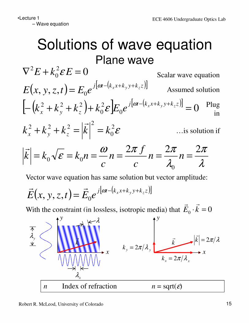
Solutions of wave equationPlane wave

15

( ) ( )[ ]

( )[ ] ( )[ ]

λ

π

λ

ππωε

ε

ε

ε

ω

ω

222

0

,,,

0

0

00

2

0

2222

0

2

0

222

0

2

0

2

======

==++

=+++−

=

=+∇

++−

++−

nnc

fn

cnkkk

kkkkk

eEkkkk

eEtzyxE

EkE

zyx

zkykxktj

zyx

zkykxktj

zyx

zyx

r

r

Scalar wave equation

Assumed solution

…is solution if

Vector wave equation has same solution but vector amplitude:

( ) ( )[ ]zkykxktj zyxeEtzyxE++−

=ω

0,,,rr

With the constraint (in lossless, isotropic media) that 00 =⋅ kErr

y

x

yλ

xλ

n Index of refraction n = sqrt(ε)

λ y

x

λπ2=kr

kr

xxk λπ2=

yyk λπ2=

Plug

in

kr

•Lecture 1

– Wave equation



Solutions of wave equationSpherical wave

16

y

x ( )222

0

222

,,,zyx

eEtzyxE

zyxktj

++=

++−ω

If you solve the scalar wave equation in spherical coordinates, you

find the spherical wave solution:

λn

ck

ω=

Ideal lenses turn portions of (infinite) plane waves into portions of

spherical waves:

Note that complex

valued, continuous field

distributions (blue) can

also be represented by

straight lines that obey

Snell’s laws (red). This is

the foundation of

geometrical optics.

•Lecture 1

– Wave equation



Geometrical opticsApprox. solution of Maxwell’s equations

( ) ( ) ( )rSjkerrE

rrrr0−= E

Assume slowly varying

amplitude E and phase S

( ) zkykxkrSk zyx ++=r

0E.g. plane wave

( ) 222

00 zyxkrSk ++=r

E.g. spherical wave

Contours of S(r) at

multiples of 2π

S∇n(r)

S(r) Optical path length [m]

“Ray” = curve ⊥ to S(r)

( )dsrn

B

A

∫=r

Ray approximation only retains information about phase

and ignores amplitude. The approximation is invalid

anywhere amplitude changes rapidly.

•Lecture 1

– Geometrical optics



Postulates of

geometrical optics

• Rays are normal to equi-phase surfaces (wavefronts)

• The optical path length between any two wavefronts is equal

• The optical path length is stationary wrt the variables that specify it1

• Rays satisfy Snell’s laws of refraction and reflection

• The irradiance at any point is proportional to the ray density at that point

•Lecture 1


1 Pedrotti3, Section 2-2



Graphical ray tracingSolving Maxwell’s Eq. with a ruler

-t t’

Object

Image

1. A ray through the center of the lens is undeviated

2. An incident ray parallel to the optic axis goes through the back focal point

3. An incident ray through the front focal point emerges parallel to the optic axis.

and occasionally useful

4. Two rays that are parallel in front of the lens intersect at the back focal plane.

5. Corollary: two rays that intersect at the front focal plane emerge parallel.

-t t’

Object

Image

0<′

=′

≡t

t

y

yM

y′−

y

•Lecture 1


Pedrotti3, Section 2-9



Graphical tracingNegative lenses

y

y’

-t

-t’

0>′

=′

≡t

t

y

yM

-f

1. A ray through the center of the lens is undeviated

2. An incident ray parallel to the optic axis appears to emerge from the front focal point

3. An incident ray directed towards the back focal point emerges parallel to the optic axis.

and occasionally useful

4. Two rays that are parallel in front of the lens intersect at the back focal plane.

5. Corollary: two rays that intersect at the front focal plane emerge parallel.

Virtual image

•Lecture 1




Spatial frequencyBasis of Fourier optics

z

xθinc

θtrans

inckr

transkr

xk

n

0λ

n

0λ

inc

xθ

λλ

sin

0=

nf transinc

x

x

00

sinsin1

λ

θ

λ

θ

λ==≡ Spatial frequency in [1/m]

transinc

x

xx nfk θλ

πθ

λ

π

λ

ππ sin

2sin

222

00

===≡ Wave number in [1/m]

The electric field of a plane wave with wave-vector sampled on a

line (the x axis) results in a sinusoidal field with spatial frequency

kr

x

xxx

kxkf

λπ

λπ

ππ

1

2

2

22

ˆ===

⋅=

r

•Lecture 1

– Fourier optics

Pedrotti3, Section 2-5, Snell’s Law



Lenses take Fourier transformsPhysical argument

E

θλλ sin=x

x

x x′F

θ

+=

=

−+ xjxj

x

xx eeE

xEE

λ

π

λ

π

λ

π

22

0

0

2

2cos

E

x′

x

FFλ

λθ 0sin =

±=

±′=

x

x

x

f

FxE

λδ

λ

λδ

1

0

0λF

xf x

′=

( ) ( )fExE →Fourier

•Lecture 1

– Fourier optics



Diffraction-limited spot size

23

′

F

dx 22

0λπ

( ) 2,, FyxE ′′

( ) 2,,0 zyE ′

′

F

dy 22

0λπ

Lens

F

d d ′

y′

z

−

F

d 2sin 1

3.83171

Neglecting diffraction, an infinitely-wide beam is Fourier transformed by a lens to an

infinitely small focused spot. Finite beams are transformed to finite focused spots.

d

Fx

dF

xf x

0

0

1 λ

λ=′→=

′=

( ) d

F

d

Fx 00 22.1

2

83171.3 λλ

π==′

From circuit theory, we know that the Fourier tranform of a rect of width d is a sinc

function with its first null at f=1/d. Let’s use this to estimate the radius of the first null

of a spot focused from a circular beam of diameter d through a lens of focal length F.

Use Fourier scale relationship

from previous page

It turns out that the 2D Fourier transform of a circ or “top hat” function is a Bessel

function – this strongly resembles a sync and is plotted above. The first null of this

“Airy disk” focused spot field distribution is

So our estimate using a rect

was only off by 20%

•Lecture 1

– Fourier optics



Numerical aperture and F/#

24

( ) 2,, FyxE ′′

The diffraction spot is the impulse response of the

optical system. The image can thus be predicted

by convolving the electric field distribution of the

object with this point spread function.

•Lecture 1

– Fourier optics

( )#22.1 0 Frspot λ=

The resolution formula is sufficiently important that several quantities are defined

to make it simpler. The F/# (pronounced “F number”) is the ratio of the focal length

to the diameter of a lens.

This is convenient because the spot radius is ~ the (F/#) expressed in wavelengths.

A similar and common quantity is the numerical aperture, which is the sin of the

largest ray angle

NAr

F

dNA spot

061.02/ λ

==

The radius of the first null is important because it defines the closest two points can

be and just be resolved (the Rayleigh resolvability criterion).

-3 -2 -1 1 2 3

0.2

0.4

0.6

0.8

1.0

Image distance in units of spot radius

|E|2

Two incoherent point sources (e.g. stars) with their

peaks on the first nulls of the adjacent point result

in a small intermediate dip in intensity.

d

FF ≡#



Laser spatial filteringRay view

Pinhole

Collimate

Objective

fobj fcol

The incident collimated beam focuses to a point which

passes through the pinhole, then expands until it hits the

collimation lens, resulting in a magnified, collimated beam.

Rays that are not collimated, representing the noise on the

beam, do not pass through the pinhole.

Pinhole

Collimate

Objective

fobj fcol

•Lecture 1

– Laser spatial filtering



Laser spatial filteringFourier optics view

Convolved with Multiplied by

= =

REAL SPACE FOURIER SPACE

•Lecture 1

– Laser spatial filtering

Documents

1: From Maxwell to Optics - University of Colorado Boulderecee.colorado.edu/~mcleod/teaching/ugol/lecturenotes/From Maxwell... · 1: From Maxwell to Optics ... Faraday’s law Ampere’s