Embed Size (px)
Citation preview
POLITECNICO DI MILANO
Scuola di Ingegneria Industriale e dell'Informazione
Corso di Laurea Magistrale in Ingegneria Elettrica
Probabilistic Production Simulation Including Wind Farms Based on
Equivalent Interval-Frequency Distribution
Relatore: Prof. Alberto Berizzi
Tesi di Laurea Magistrale di:Jin LanjuMatr. 10431698
Anno Accademico 2014-2015


ABSTTRACT
ABSTRACT
Abstract in italiano
La tradizionale simulazione probabilistica di produzione dei sistemi elettrici di potenza si
basa sulla curva di durata del carico per descrivere le proprietà temporali del carico. Tuttavia,
questa descrizione manca delle informazioni sulle fluttuazioni del carico e dei vincoli
temporali relativi alla caratteristica cronologica, ciò si traduce nel fatto che non tiene conto
dei tempi minimi e massimi, delle restrizioni sulle rampe, dell’organizzazione dei generatori
e di altri fattori nel processo di simulazione. Il metodo tradizionale non è in grado valutare il
costo dinamico di avvio e di arresto delle unità causato dalla fluttuazione del carico e di
conseguenza la valutazione risulta relativamente approssimata. Con la crescente diffusione
delle tecnologie non programmabili, come l’eolico, la crescente fluttuazione di carico
produrrà un impatto maggiore. Pertanto abbiamo bisogno urgentemente di studiare la
simulazione probabilistica di produzione che è in grado di fornire una valutazione più
globale.
Il metodo di frequenza e durata (FD) impiega la curva di frequenza di carico per rispecchiare
i fattori di fluttuazione sopracitati, corrispondenti alla frequenza di operazioni di avvio e di
arresto delle unità. Tuttavia FD ignora l’impossibilita di avvio e arresto negli intervalli brevi
di tempo, portando cosi ad uno scostamento nel risultato. Al fine di riflettere maggiormente
le caratteristiche cronologiche del carico e ottenere un risultato più realistico, in questa tesi la
curva di frequenza di carico è estesa alla distribuzione degli intervalli di frequenza e alla
serie della distribuzione degli intervalli di frequenza, che coinvolge sia le informazioni sulla
frequenza sia le informazioni sulla distribuzione temporale delle fluttuazioni del carico. Più
dettagliatamente, la frequenza di transizione di ogni livello di carico viene espansa in una
serie di intervalli temporali, utilizzando una struttura di tempo per registrare ciascun
intervallo adiacente di tempo di trasferimento. Poi, analogamente alla derivazione delle
curve di durata del carico effettivo (ELDCs) nei costi Bleriaux-Booth, la distribuzione di
frequenza dei carichi effettivi, con le informazioni dei rispettivi intervalli di tempo, può
essere valutata con il processo di convoluzione, che può essere considerato come una
modifica di ogni struttura temporale. In questo modo, viene sviluppato il metodo di
I

ABSTTRACT
simulazione di produzione probabilistico basato sull’equivalente distribuzione di intervalli di
frequenza. Le informazioni cronologiche sia dei carichi che dei parchi eolici possono essere
coinvolte, in una certa misura, sulla base delle informazioni di intervallo di tempo delle
strutture temporali effettive. In più, l'effetto dell’energia eolica viene valutato più
ragionevolmente per quanto riguarda i costi dinamici.
L'impatto dei parchi eolici sull'affidabilità metrica, più olistiche informazioni di costo
comprensivo del costo del carburante, costi ambientali e costi dinamici saranno discussi con
l'algoritmo presentato e il sistema di test integrato EPRI-36 per l’eolico. Anche l'impatto
dell’energia eolica sui costi dinamici è studiato. Esempi numerici dimostrano che questo tipo
di algoritmo è più vicino alla realtà e più accurato rispetto ai metodi FD.
Abstract in inglese
The traditional probabilistic production simulation of power system is based on the load
duration curve to describe the temporal property of the load. However, this derived
description misses the load fluctuation information and time constraints related to the
chronological characteristic, which is resulting in the fact that it fails to take consideration of
the minimum up time and minimum down time limit, ramping rate restriction, generator
scheduling, and other factors in the production simulation process. The traditional way can
not evaluate the dynamic cost of unit startup and shutdown caused by the load fluctuation
and the assessment is relatively rough as a result. With the increasing penetration of non-
dispatchable technologies, such as the wind power, more impact will be produced by the
growing fluctuation of net load. Therefore urgently we need to study the probabilistic
production simulation which can provide a comprehensive assessment.
The frequency and duration (FD) method employes the load frequency curve to reflect the
above fluctuation factors, corresponding to the frequency of unit startup and shutdown
operation. But it ignores the infeasibility of the startup and shut down in short time interval,
which also leads to a deviation in the result. In order to reflect more chronological load
characters and get a more realistic result, in this thesis the load frequency curve is extended
II

ABSTTRACT
to the interval frequency distribution and interval frequency distribution series, which
involves both the frequency information and time distribution information of load
fluctuation. In more details, the transition frequency of every load level is expanded into a
time interval series, by using a time structure to record each time interval of adjacent upward
transfer and downward transfer. Then analogously to the derivation of Effective Load
Duration Curves (ELDCs) in Bleriaux-Booth costing, the effective load interval frequency
distribution function with the information of respective time interval can be evaluated
through the convolution process, which can be regarded as a modification of each time
structure. In this way, the probabilistic production simulation method based on the equivalent
interval frequency distribution is developed. The chronological information of both the load
and wind farms can be involved to a certain extent based on the time interval information of
effective time structures. What’s more, the effect of wind power is also evaluated more
reasonably with the respect to the dynamic cost.
With the presented algorithm and the wind power integrated EPRI-36 test system, the impact
of the wind farms on reliability metric and more holistic cost information including fuel cost,
environmental cost and dynamic cost will be discussed, and the impact of the wind power
scale on dynamic cost rate is also studied. Numerical examples demonstrates that this kind of
algorithm is more close to reality and more accurate compared to the FD methods.
III

Index of Tables
List of Main Symbols
mn
The upward load transfer duration [h]The downward load transfer duration [h]The first type of time structure which indicates the upward transfer frequency of load level k, of which the front and back adjacent time interval is m and n, respectivelyThe second type of time structure which indicates the downward transfer frequency of load level k, of which the front and back adjacent time interval is n and m, respectivelyThe first type of interval-frequency distribution series made up
of time structure The second type of interval-frequency distribution series made
up of time structure The whole combined interval-frequency distribution series of load level kThe load step in the simulation processThe total number of unitsThe corresponding discrete values of maximum load in the initial systemThe capacity of i-th unitThe corresponding discrete values of i-th unit capacity,
The loading position for i-th unit,
The discrete value of total installed capacity, The equivalent interval-frequency distribution series after arranging the first i-1 unitsThe first equivalent time structure of the interval-frequency distribution after loading the perivous i-1 unitsThe second equivalent time structure of the interval-frequency distribution after loading the perivous i-1 units
IV

Index of Figures
The minimum up time of i-th unit
The minimum down time of i-th unit
The expected startup frequency of i-th unit
The expected shutdown frequency of i-th unit
The expected removed startup frequency of i-th unit
The expected removed shutdown frequency of i-th unit
The generator startup and shutdown of unit capacity,
The Short Time Interval Proportion of Unit Capacity
The short time interval dynamic cost
V

Index of Tables
Index of Figures
Fig. 2-1 Daily duration load curve...........................................................................................8Fig. 2-2 Duration load curve explaination...............................................................................8Fig. 2-3 Daily chronological load curve and its duration load curve.......................................9Fig. 2-4 24h original load, net load and wind power.............................................................10Fig. 2-5 The comparision of the load frequency curve..........................................................10Fig. 2-6 The 24h original net load curve................................................................................11Fig. 2-7 The geometric explaination of time structure...........................................................13Fig. 2-8 The interval-frequency distribution of load level k..................................................15Fig. 2-9 The original load data of the simple example..........................................................16Fig. 2-10 The original chronological net load curve..............................................................16
Fig. 2-11 The segmentation of first type of time structure for load level 4150MW.........................................................................................................................................18
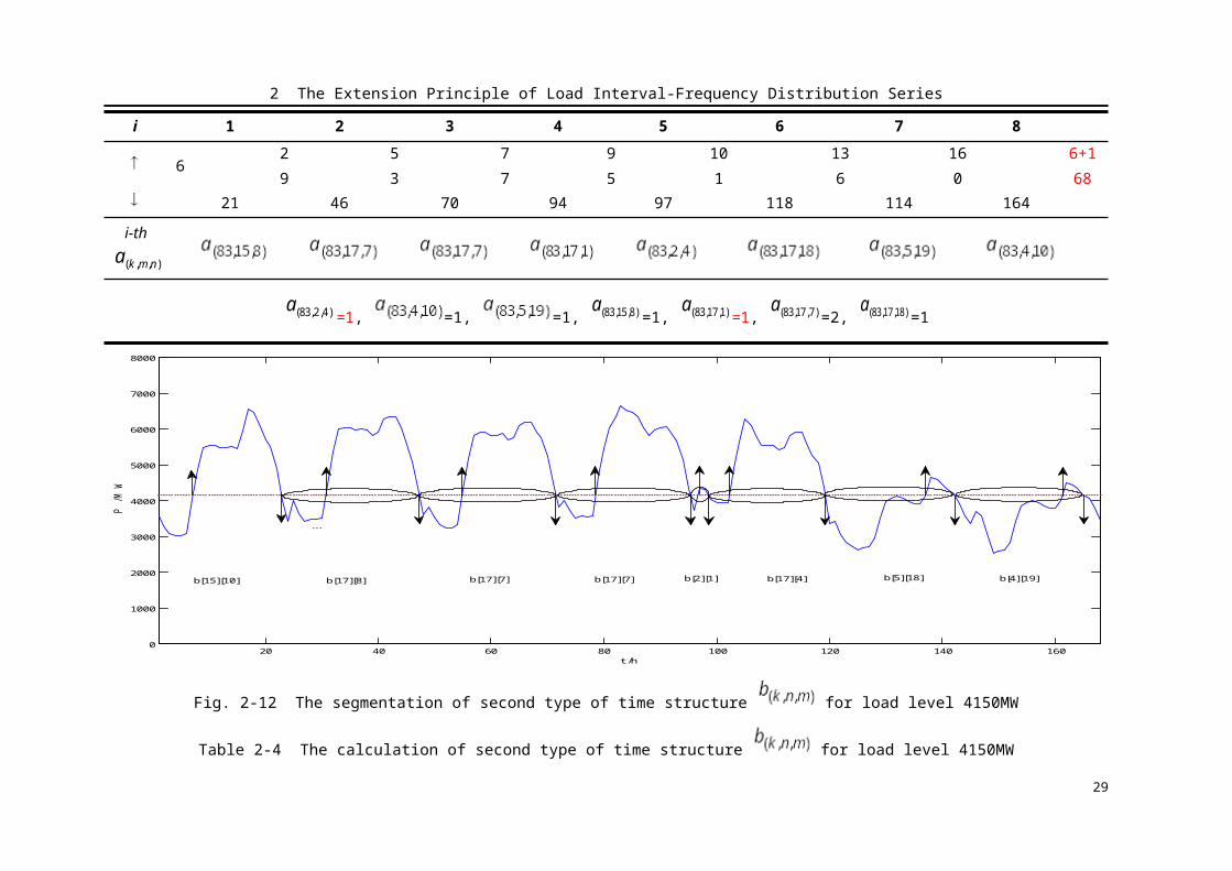
Fig. 2-12 The segmentation of second type of time structure for load level 4150MW.........................................................................................................................19
Fig. 2-13 The interval-frequency distribution of load level 4150MW...................................20Fig. 2-14 The comparison of the original load frequency curves..........................................20Fig. 3-1 The lifetime processes and state diagram of generator............................................22Fig. 3-3 The form of equivalent energy function...................................................................24Fig. 3-4 The form of equivalent load frequency curve..........................................................25Fig. 3-5 The explaination of discrete energy function...........................................................30Fig. 3-6 The geometric interpretation for i-th unit energy calculation...................................31Fig. 3-7 The time structure to analyse the startup and shutdown response............................34Fig. 3-8 Flow chart of the probabilistic production simulation.............................................38Fig. 4-1 IEEE RTS load date and wind power.......................................................................40Fig. 4-2 The original load frequency curve............................................................................43Fig. 4-3 The detailed convolution process without wind power............................................44Fig. 4-4 The detailed convolution process with wind power.................................................44
Fig. 4-5 The equivalent interval-frequency distribution of 4400MW with and without wind power........................................................................................................47
Fig. 4-6 The equivalent interval-frequency distribution of 4400MW with and without wind power........................................................................................................48
Fig. 4-7 The relationship between short interval dynamic cost and the number of wind turbines............................................................................................................................57
VI

Index of Figures
Fig. 4-8 The relationship between short time interval proportion of unit capacity...............57Fig. 4-9 The relationship between dynamic cost rate and the number of wind turbines.......58Fig. 4-10 The relationship between generating cost and the number of wind turbines.........58
VII

Index of Tables
Index of Tables
Table 1-1 Planning and construction of wind power bases..............................................2Table 2-1 The transfer moment of load level 4150MW.................................................17
Table 2-2 The calculation of first type of time structure for load level 4150MW.................................................................................................................18
Table 2-3 The calculation of second type of time structure for load level 4150MW.................................................................................................................19
Table 3-1 The calculation process of i-th unit production simulation...........................27Table 3-1(continued) The calculation process of i-th unit production simulation.........28Table 3-1(continued) The calculation process of i-th unit production simulation.........29Table 4-1 The parameter of wind turbines.....................................................................41Table 4-2 The data of generator system EPRI-36..........................................................41Table 4-2(continued) The data of generator system EPRI-36........................................42Table 4-2(continued) The data of generator system EPRI-36........................................42Table 4-3 The equivalent interval-frequency distribution of 4400MW without wind
power.......................................................................................................................45Table 4-4 The equivalent interval-frequency distribution of 4400MW with wind power
.................................................................................................................................49Table 4-4(continued) The equivalent interval-frequency distribution of 4400MW with
wind power..............................................................................................................50Table 4-5 The statistics of equivalent time structure of 4400MW.................................50Table 4-6 The comparison of unit expected energy with wind power...........................51Table 4-7 The comparison of reliability index with wind power...................................51Table 4-8 The expected startup frequency of each unit.................................................52Table 4-8(continued) The expected startup frequency of each unit...............................53Table 4-9 The expected shutdown frequency of each unit.............................................53Table 4-9(continued) The expected shutdown frequency of each unit..........................54Table 4-10 The comparison of each dynamic cost index...............................................54Table 4-11 Probabilistic production simulation results based on interval-frequency
distribution..............................................................................................................55
VIII

Contents
Contents
ABSTRACT..............................................................................................................................IList of Main Symbols.............................................................................................................IVIndex of Figures......................................................................................................................VIIndex of Tables.....................................................................................................................VIIIContents..................................................................................................................................IX1 Preface....................................................................................................................................1
1.1 Background and Motivation............................................................................................11.2 Status of Production Simulation with wind power.........................................................41.3 Main Contents of the Study............................................................................................5
2 The Extension Principle of Load Interval-Frequency Distribution Series.............................72.1 Brief Introduction............................................................................................................72.2 Load Duration Curve and Load Frequency Curve..........................................................72.3 Load Interval Frequency Distribution Series................................................................12
2.3.1 The Extension Principle.........................................................................................122.3.2 Simple Example Aanlysis......................................................................................15
2.4 Brief Summary..............................................................................................................213 Probabilistic Production Simulation Based on Equivalent Interval Frequency Distribution.................................................................................................................................................22
3.1 Profile of Power System Probabilistic Production Simulation.....................................223.2 Probabilistic Production Simulation Based on Equivalent Interval Frequency Distribution.........................................................................................................................273.3 Assessment Model of Probabilistic Production Simulation..........................................30
3.3.1 Generator Production and Reliability Index..........................................................303.3.2 Generator Expected Startup Frequency.................................................................323.3.3 Dynamic Costs.......................................................................................................35
3.4 Calculating Flow of Probabilistic Production Simulation............................................383.5 Brief Summary..............................................................................................................38
4 Case Studies.........................................................................................................................404.1 Basic Data.....................................................................................................................40
4.1.1 Load Data...............................................................................................................404.1.2 Generator Data.......................................................................................................41
4.2 Result of Probabilistic Production Simulation..............................................................424.2.1 Analysis of Equivalent Interval Frequency Distribution........................................424.2.2 Analysis of Probabilistic Production Simulation...................................................51
4.3 Assessment of Dynamic Costs......................................................................................524.3.1 Analysis of Generator Expected Start-up Frequency.............................................524.3.2 Analysis of Dynamic Costs....................................................................................54
IX

Contents
4.3.3 The Influence of Wind Capacity............................................................................565 Conclusions..........................................................................................................................59References...............................................................................................................................61Research Achievements during the study...............................................................................64
X

2 The Extension Principle of Load Interval-Frequency Distribution Series
一 Preface
一.1 Background and Motivation
In today's society with the increasing environmental conditionality and decreasing
natural resources. The market-oriented reforms of power industry is in a accelerating
process. For the formulation of effective planning, how to take full consideration of power
supply structure optimization adjustment is the key point in energy saving electricity
production with higher requirements so that it can provide a great decisive and policy
support for the power industry more scientific, efficient, economic, sustainable, coordinated
development.
Recently China's power industry is develop rapidly. The annual growth rate of power
generator installed capacity and power generation is reaching 10.5% and 10.34%,
respectively. The current total installed capacity is ranking in the second place in the world,
just after the United States [2]. However, the production of electricity is mainly through coal,
in which the coal-fired electricity generation is accounting for about 75% and the numerous
fossil fuel consumption and heavy environment pollution is becoming a great bottleneck,
severely restricting China's economic growth. To adjust and optimize the energy structure,
exploring new energy sources and recycling energy, is an important security and energy
sustainability policy for healthy development. Wind power is belonging to a kind of
renewable energy, which is also favorable to environmental protection. Not only it does not
require to burn fossil fuels, but also it will not cause any air pollution. Therefore, more and
more attention is taken in the research of wind power around the world. Meanwhile, wind
power has a huge reserve. According to the incomplete statistics, the total global wind
resource is not less than 2.74×10⁶GW, of which, for the development and utilization of wind
energy is accounting for 2×10⁴GW. China's wind energy reserve is distributed in a wide area,
merely it has approximately 2.53×10²GW on land, indicating a bright development potential
and prospect. In today’s society, the problem of environmental pollution and energy
sustainability is growing more serious. Meanwhile the electricity market is in the gradual
deepening of reform. The utilization of renewable energy for power generation in the world
have become a hot topic, and also have a rapid development, especially, for the wind power,
1

2 The Extension Principle of Load Interval-Frequency Distribution Series
it is one of the fastest growing power generations and it is also the most mature and
advanced at the technical level.
During the "Eleventh Five Year Plan", China's wind power has been developed rapidly
[2]. According to official statistics, our total installed capacity of wind power in 2013 is
already reached as much as 74.58GW and it is increased into 90GW, of which wind power
generating capacity is 15.63 billion kwh, with an increase by 12.2% [6]. Wind power
equipment utilization hours are as high as 1905 hours. In addition, there is an ambitious
objective for the development of the new energy source in future. By 2020, the wind power
capacity will plan to increase from 30GW to 150GW. Among them, the Jiangsu wind power
base of million kilowatts in 2015 has the installed capacity of 3.8GW [3], and the target for
2020 target is to improve into 10GW of wind power capacity. Jiuquan wind power base of
million kilowatts in 2011 has the installed capacity of 4.201GW [5], and it is planned to
reach 12.71GW in the "Twelfth five Year Plan", which will become one of the world's largest
wind power bases. Table 1-1 shows eight 10GW wind power bases under planning and
construction from the National Development and Reform Commission [7]. In 2020, the total
capacity of these eight wind power bases will exceed 120GW.
Table 1-1 Planning and construction of wind power bases
Location Planned capacity [GW] Grid to be connected
Gansu Jiuquan 12 Northwest Grid
Xinjiang Hami 20 Northwest Grid
Mongolia west 20 North China Grid
Mongolia east 30 Northeast Grid
Hebei north 10 North China Grid
Jiangsu 10 East China Grid
Jilin 10 Northeast Grid
Shandong 15 North China Grid
While the wind power penetrates the power system for its clean and renewable benefits,
its effect on the aspects of power system operation and planning will become increasingly
prominent. Due to the stochastic volatility of the wind power, not only the reverse power
pressure is enlarged, but also the startup and shutdown operations of conventional units to
meet the fluctuated net loads are becoming more frequently, which leads to increment of
2

2 The Extension Principle of Load Interval-Frequency Distribution Series
relevant dynamic costs. Moreover, the wind farm output at night is generally greater than
that one during the day, also greater in winter more than one in summer, which is just exactly
the opposite to the normal changing law of system load. What is worse, wind turbines have a
poor control and this anti-peaking property is likely to increase the equivalent gap of the
peak and valley load. All in all, the high volatility and intermittency of wind power output is
bring new difficulties to the entire power system dispatch, probably making the system
operation further deteriorate.
Reference [8] and [9] employed the measured data in the Jiuquan wind power base to
study the wind power output characteristics and note that the wind power output has obvious
relevance and require more conventional power generators for peaking plan, considering
from the long time scales. Reference [10] pointed that after the wind power with 5160MW
installed capacity access the Gansu Power Grid, the gap between the peak load and valley
load became almost three times of that one without wind power. The monthly average peak-
valley difference rate in Gansu power grid 2010 is close to or exceeds the maximum
regulating peak load ability in the case when the thermal power generators are not allowed to
startup and shutdown in one day. Hence, the coordination of the conventional unit startup
and shutdown and the peak regular is becoming significantly frequently in the power system
including wind farms, which will definitely increase a lot in the dynamic cost of
consumption. Wind power penetration will extremely increase the additional cost.
Accordingly, the impact of wind power on the power system cannot be ignored and we need
to make the scientific and rational deployment planning to develop these renewable energy
sources.
As one of the significant methods for improvement and optimization of power system
production, stochastic production simulation is comprehensively considering both of the load
variation and random generator fault for the calculation of production costs and reliability
analysis, under the optimal operation based on the predicted future load curve. Its core
mission is to carry on operating mode analysis, production cost calculation and reliability
evaluation. Basic functions can be broadly grouped into the following aspects [19]:
(1) provide the expected production energy for each plant, the fuel consumption and
the corresponding fuel costs during the simulation under optimum operating mode;
(2) compute power system reliability indicators in this operating mode, for example,
the Expected Energy Not Supplied (EENS) and the Loss of Load Probability (LOLP);
3

2 The Extension Principle of Load Interval-Frequency Distribution Series
(3) analyze the whole production cost in this simulation, including the environmental
cost, the customer interruption cost and so on.
Stochastic production simulation is playing an important role in assessing the future
development of the power system to improve economic efficiency and supply reliability
level of power system operation. As an important way to evaluate the reliability and
production cost, it is quite necessary to consider the impact brought by wind power volatility.
If the timing information of wind power can be also modeled in the processing, it will help to
get a more accurate evaluation with a full point of view.
一.2 Status of Production Simulation with wind power
As for the production simulation for power system, domestic and foreign scholars
already have done a lot of research, which generally can be divided into two types of
simulation model-- stochastic production simulation and probabilistic production simulation
[22].
Stochastic production models is simulating directly in the chronological load curve. The
main method is called Monte Carlo and Markov [16]. Through detailed statistics of
frequency of each incident, Monte Carlo can make the deep estimation of system state.
However, the convergence speed is proportional to the square root of sample size, resulting
in a large computation and certain randomness, which limits the widespread use of such
methods. The core of probabilistic production simulation is to transform the timing load
curve into the Load Duration Curve (LDC) and the effect of random outages of generating
units is considered as the increase of system load to form the equivalent load duration curve.
It reflects that after the unit is outage with certain probability, the rest of other units will face
a relatively large equivalent load duration curve, namely, to bear more load. Probabilistic
model was first introduced by Baleriaux in the 60s [15], Booth continued to improve it,
thereby the famous Baleriaux-Booth model and algorithm were formed, of which the key is
to convolute standardly the probabilistic random variables of distribution function in the
simulation. Around how to describe the timing load curve and how to improve the speed and
accuracy of convolution and deconvolution calculation, scholars made a lot of
improvements. Typical algorithms are [19]: Piecewise Linear Approximation Method, the
Cumulant Method [17], the Method of Moments [18], Mixture of Normal Approximation
Method (MONA), Fast Fourier Transform Method (FFT) and Equivalent Energy Function
4

2 The Extension Principle of Load Interval-Frequency Distribution Series
(EEF) [20] [21] and so on.
However, the load duration curve lose part of timing information of system load and
can not include the time-dependent constraints, such as unit commitment fee, the minimum
time requirement of startup and shutdown, ramp rate constrain of thermal power units, etc.
The conventional unit startup and shutdown cost, hot standby and other dynamic
characteristics and dynamic cost are not taken into consideration in the simulation process,
leading to the sad fact that production costs are relatively sketchy.
Extensive literatures [10]-[12] discussed the establishment of the wind farm model
reliability or peaking related strategies, but for wind power planning including economic
evaluation of unit startup and shutdown, power reserves and peaking regulation, it is poorly
studied. When penetrating large-scale wind power under priority consumptive principle, the
system load volatility is strengthened a lot and the peak-valley difference is also growing,
which means a corresponding increase in conventional unit startup and shutdown operation
and dynamic cost. How to assess the dynamic cost so as to make the power planning run into
a meaningful surface for a comprehensive analysis of the production costs, evaluation of the
wind farm effectiveness and determination of wind power capacity is quite crucial. The
traditional simulation algorithm is no longer able to meet the practical requirements of the
power system in the production cost assessment to a certain degree.
Literatures [33]-[38] proposed a method based on the load frequency curve, namely
Frequency and Duration Method (FD). It employs the load frequency curve (LFC) instead of
the load duration curve to describe the load timing characteristics to consider more timing
related information. Among them, the literature [37] and [38] combine the EEF method with
the load frequency curve to evaluate the production simulation. The FD method reflects part
of the timing fluctuation of frequency information, but at the same time it misses the timing
distribution fluctuations, causing that the dynamic costs of startup and shutdown in short
time interval in the simulation process is also included when assessing the whole production
costs. It fails to accord with the practical operations and introduces a potentially significant
bias inaccuracy in assessment. With the increasing penetration of non-dispatchable
technologies, such as the wind power, this error will become more apparent.
5

2 The Extension Principle of Load Interval-Frequency Distribution Series
一.3 Main Contents of the Study
In order to reflect more chronological load characteristics for a more reasonable
dynamic cost, this thesis introduces the interval frequency distribution series based on load
transfer(hereinafter referred to as the interval-frequency distribution), as an extension of load
frequency curve. Composed of time structures, the interval-frequency distribution not only
contains all the information in the load frequency curve, but also to a certain extent reflect
the timing distribution of load fluctuation, providing more basis when assessing the dynamic
cost of unit startup and shutdown caused by the penetration of wind power. A new
probabilistic production costing is studied just based on this new description of load curve.
Specific work completed in this thesis is as follows.
(1) for the time-varying characteristics of the load, the load frequency curve will extend
into the load beyond the interval-frequency distribution in the form of time structure, not
only to cumulate the number of load transfers, but also to maintain recording two adjacent
time intervals of each load transfer, reflecting both the timing fluctuation frequency
information and time distribution of information.
(2) Analog to frequency and duration curve, develop the new probabilistic production
simulation algorithm based on the establishment of equivalent interval-frequency
distribution. By standard convolution, the random failure influence of unit is considered as
the continually updated equivalent interval-frequency distribution series of the previous one.
Based on the detailed information contained in each corrected time interval, the expected
power generation, system reliability, the frequency of unit startup and shutdown and related
dynamic costs are respectively elaborated in the evaluation system.
(3) Combined with EPRI-36 system and the IEEE RTS, simulate the production in the
first 30 days of one month with proposed method, where the wind farm refers to the
historical data of Da Ban Cheng region. Assess the production cost based on the equivalent
interval-frequency distribution. Then analyze and compare the results with the one in
equivalent energy function method, frequency and duration method to verify the validity and
accuracy of the proposed method. Finally, the influence of the wind power penetrated scale
on the entire power system will be also studied.
6

2 The Extension Principle of Load Interval-Frequency Distribution Series
二 The Extension Principle of Load Interval-Frequency Distribution Series
二.1 Brief Introduction
Power System Probabilistic Production Simulation is a kind of algorithm, which is
based on considering both random failures of units and the system load fluctuation, aiming
to calculate the expected energy for each plant, the production costs and system reliability
indices in the optimum operating mode. As it is well-known, the timing fluctuation of system
load leads to the startup and shutdown operations of units to balance the whole system,
which will result in the so-called dynamic costs. With the increasing amounts of intermittent
energy access, the volatility of the system will be further improved and the dynamic
operation of the conventional units will become more frequent. Timing fluctuations
information is including both the fluctuated frequency and the distribution of the fluctuation.
If these information is more completed reflected in the simulation, it will help a lot to
characterize and describe some relevant phenomena. Therefore, how to accurately describe
the load characteristics and give a full consideration to the timing fluctuation of the system is
one of the key issues to get a comprehensive assessment of probabilistic production
simulation. 112Equation Chapter 2 Section 1
二.2 Load Duration Curve and Load Frequency Curve
Generally speaking, the chronological load curve in the traditional method is converted
into the duration curve to describe the characteristics of system load. Instead by the time
increments, the duration curve is ordered by the duration of each load level in the whole
study period. Depending on the study period, it can be classified into daily, weekly, monthly,
and annual duration curve. Fig. 2-1 shows the relationship between the daily load curve and
the corresponding duration load curve, and the time relation in x axis of each load level is
always satisfying the formula (2-1).
222\* MERGEFORMAT (-)
7

2 The Extension Principle of Load Interval-Frequency Distribution Series
Where:
——the j-th duration of load in the chronological load curve;
——the total duration of load .
Fig. 2-1 Daily duration load curve
For example, in Fig. 2-1, there exists this kind of relationship, . Typically,
the duration load curve can be obtained by rotating these two coordinates in Fig. 2-1. As
shown in the Fig. 2-2, which presents a daily duration load curve, the x axis means the load
level and the y axis represents the corresponding duration. T means the study period,
is the maximum load for the system. At any point (x, t) in the curve, it indicates the duration
of system load which is equal or greater than x is equal to t, i.e.,
323\* MERGEFORMAT (-)
8

2 The Extension Principle of Load Interval-Frequency Distribution Series
Fig. 2-2 Duration load curve explaination
Obviously, such derived method above would result in loss of part of load time
information, such as the load fluctuation information, making it impossible to involve the
related dynamic costs of generator count in probabilistic production simulation. Fig. 2-3(a)
shows two different timing load curve and , converting into the load duration
curve using the method above, both of these two duration load curves are exactly the same
[37], as shown in Fig. 2-3(b). However, there is no doubt that the fluctuation frequency and
amplitude of the load curve is much larger than the load curve . Obviously, the
startup and shutdown operations of unit with system is more frequently and it costs
more in the aspect of warm-up, maintaining the operating reserve which is related to the
dynamic factors.
9

2 The Extension Principle of Load Interval-Frequency Distribution Series
Fig. 2-3 Daily chronological load curve and its duration load curve
The load frequency curve is firstly introduced to regard the chronology of events. It
represents the average frequency in the study period with which load level is crossed in an
upward direction of the chronological curve, i.e., the load is in transition from lower one to
higher one. What’s more, it’s exactly equal to the average frequency with which load level is
crossed in an downward direction. Assume that is the average times of upward cross of
load level k, then its corresponding load frequency is
424\* MERGEFORMAT (-)
Fig. 2-4 illustrates one typical day (24h) load data that includes the original load, wind
power output and net load. Take the example of load level of 6000MW. Scanning the load
curve from the beginning in the original load curve, the load is 5516MW at 7:00 and
increases to 6182MW at 8:00. And the upward transfer happens only once over the study
period. Therefore, the original frequency in the 6000MW load level is 1/24. Similarly, all the
other load frequency can be obtained in this way and the corresponding original load
frequency curve is shown in Fig. 2-5, where x axis is the system load and y axis is
corresponding load transfer times. By subtracting the initial load from the intermittent wind
power output to consider the impact of intermittent energy sources, we can get the net load
curve as the basis of generation of original load frequency curve. Compared with the original
load curve in Fig. 2-4, the net load curve obviously has more volatility and in the
corresponding load frequency curve, the total load transfer frequency is significantly
increased, at the same time the mainly distributed load interval is also changed.
10

2 The Extension Principle of Load Interval-Frequency Distribution Series
0 5 10 15 20 250
1000
2000
3000
4000
5000
6000
7000
t /h
P /M
W
original loadwind power
0 5 10 15 20 250
1000
2000
3000
4000
5000
6000
7000
t /h
P /M
W
net load
Fig. 2-4 24h original load, net load and wind power
0 1000 2000 3000 4000 5000 6000 7000 8000 9000 100000
0.5
1
1.5
2
2.5
3
3.5
4
4.5
x /MW
load
tran
sitio
n fre
qunc
y /ti
mes
Net loadOriginal load
Fig. 2-5 The comparision of the load frequency curve
The Frequency and Duration method is using load frequency curve to reflect the partial
load timing information. And through convolution, the equivalent load frequency curve is
obtained to correspond the frequency information of the unit startup and shutdown, hence in
that way the related dynamic costs are evaluated. Fig. 2-6 illustrates the principle about how
the load frequency curve responds to conventional unit commitment. Suppose unit N is
loading at the load level 6000MW, the system load is less than 6000MW before 8:00 without
accessing the wind power, obviously this unit N is in shutdown state or hot standby.
However, when the system load is growing greater than 6000MW after 8:00, accordingly
this units N should be switched on, that is to say, the load upward shift corresponds to one
11

2 The Extension Principle of Load Interval-Frequency Distribution Series
time of startup process. Also, before 22:00, since the system load is always greater than
6000MW, where unit N will have to keep on. Until after 22:00, the system load decreases,
this unit will be shut down or reduce output to keep a hot spare.
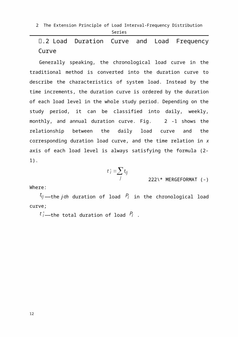
In the FD method, the load frequency curve directly reflects the demand of unit startup
and shutdown. When the corresponding loading level is transferring upward, it means the
desired unit starts while when the load level is downward transferring, the unit shutdown
will be issued. Obviously, the FD method does not take into account the feasibility of
continuous startup and shutdown in the short interval, which will introduce a lot of error
compared with the actual situation. With the increasing of the intermittent energy access, the
system volatility will be further improved and this kind of phenomenon is becoming more
notable.
0 5 10 15 20 250
1000
2000
3000
4000
5000
6000
7000
t /h
P /M
W
original loadwind powernet load
Fig. 2-6 The 24h original net load curve
After the access to wind power, not only the frequency of load fluctuations is increased,
but also the interval of adjacent load transfer tends to decrease greatly. Once again, take the
example of 6000MW load level as shown in Fig. 2-6. There exist totally three times of load
upward transfers occurred in the net load curve, respectively, at 9:00, 13:00 and 16:00.
Meanwhile, there are also three times of load downward transfers. Obviously, the interval
between adjacent load transfers is quite small, where the smallest one is only 1 hour.
If it goes with one correspondence between the transfer frequency and unit operation,
there would be three expected demands of unit startup and shutdown, respectively to be
12

2 The Extension Principle of Load Interval-Frequency Distribution Series
included in the evaluation of dynamic costs. However, if the generator has to be started up in
a longer time interval, which means the operating limits or the down time limit is large, it is
more likely to choose some time to maintain output state, rather than frequently start up or
shut down. Relying merely on the frequency of the load fluctuations seems inadequate, more
information is needed for calculation and evaluation.
For each load level, there exist two intervals between the upward transfer and its
adjacent downward transfers, also two intervals between the downward transfer and it
adjacent upward transfers. In actual operation, for the unit startup operation, only when both
of these two intervals of upward transfer satisfy the time limits, i.e., the minimum up time
and minimum down time, the request of unit startup can be fulfilled. Similarly, only when
both of these two intervals of downward transfer satisfy the time limits, the request of unit
shutdown can be fulfilled. For this reason, by recording each interval of load transfer, the
load frequency curve is extended to the interval-frequency distribution series, which can
both reflect the frequency information and distribution of timing information, more fully
considering the timing characteristics of load fluctuation. Then the probabilistic production
simulation method based on the equivalent interval frequency distribution is developed to
give a more reasonable assessment of dynamic costs.
二.3 Load Interval Frequency Distribution Series
二.3.1 The Extension Principle
In order to obtain the time interval between each load transfer, for each load level k,
while scanning the original load timing curve, not only it needs to cumulate load transfer
frequency, but also every upward and downward transfer moment is recorded. Set the period
between two adjacent upward transfers as one time structure and calculate the inside two
time intervals, respectively denoted as m and n, the item m represents the load upwards
duration, n is the load downwards duration and their unit depends on the time step, usually
it’s recorded by hour. Meanwhile, set the period between two adjacent downward transfers as
another time structure and calculate the two time intervals inside, respectively denoted as n
and m, the item m can still represent the load upwards duration and n is the duration of the
downward transfer as shown in Fig. 2-7. Thus, for the load level k, we can get two different
time structures, and are counted as and Each time structure contains two
13

2 The Extension Principle of Load Interval-Frequency Distribution Series
time intervals, i.e., load upward transfer duration m and downward duration n. Time
structure describes the downward transfer of load level k with which the adjacent
front and back time interval is respectively m and n. According to the minimum up time and
minimum down time of the corresponding unit, it can be used to determine the response of
unit shutdown. While time structure describe the upward transfer of load level k
with which the adjacent front and back time interval is respectively n and m to determine the
demand of unit startup.
Fig. 2-7 The geometric explaination of time structure
For each load level, the frequency of load upward transfer within the study period is
exactly equal to the one of downward transfer. Therefore, the total value of both time
structure are the same and equal to the corresponding load frequency in the load frequency
curve. In order to depict each time interval of load transfer simultaneously, we add these two
time structure values, then divide by 2 so that the numerical value can be in accord with the
load frequency curve. Thus, the combined structure can be obtained and denoted as
in this thesis to describe the interval-frequency distribution of load level k. In the discrete
case, assuming that the time step is an integer value of 1 hour, load step size is an integer of
1 MW. At this moment, the interval-frequency distribution for load level k can be
represented as follows:
14

2 The Extension Principle of Load Interval-Frequency Distribution Series
525\*MERGEFORMAT (-)Where,
M——the maximum time interval of load upward duration; N——the maximum time interval of load downward duration.
Element represents the downward transfer frequency of load level k with
which the two adjacent time intervals are m and n, and the other element represents
the upward transfer frequency of load level k with which the two adjacent time intervals are
n and m. They are together to reflect the interval-frequency distribution for load level k. In
the study period T, the last transfer is connected with the first one to make up another time
structure. For the zero transfer load, i.e., the base load, the time structure can be expressed as
, or which means the load upward duration is the study period T. In
addition, the following relationships are valid for all load levels, i.e., the sum of all the time
intervals of time structures is just equal to the entire study period T.
626\*MERGEFORMAT (-)
For all load levels within the study scope, the interval-frequency distribution can be
formed, which corresponds to the frequency curve. The whole interval-frequency of
distribution. can be expressed as two three-dimensional arrays:
727\* MERGEFORMAT (-)Where:
K——is the discrete values of maximum system load.
Each element in the three-dimensional array represents one time structure. That is to
say, is meaning the element of which three-dimensional parameters are k, m, and n.
In order to visualize corresponding interval-frequency distribution for load level k, put the
15
2 The Extension Principle of Load Interval-Frequency Distribution Series
time structure into the spatial coordinate as shown in Fig. 2-8. The horizontal axis and the
vertical axis in the bottom represents the load upward duration and downward duration,
respectively. The vertical axis represents the corresponding frequency, i.e., the value of
and . A similar chart can be done for each load level k.
Fig. 2-8 The interval-frequency distribution of load level k
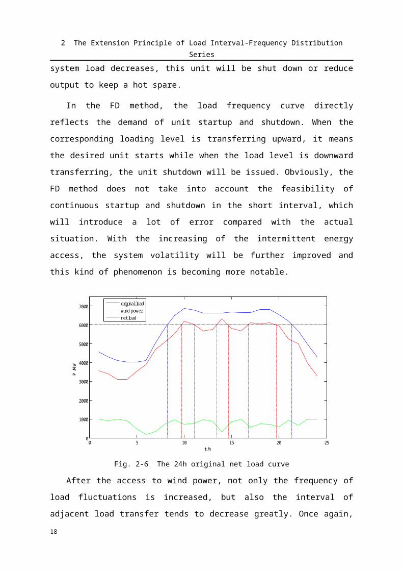
二.3.2 Simple Example Aanlysis
To further explain the extension principle of interval-frequency distribution series, this
section illustrates one simple example of one week load (168 hours) for analysis where load
step is taken as 50MW and discrete time value is 1h, the original load data shown in Fig. 2-9.
16

2 The Extension Principle of Load Interval-Frequency Distribution Series
20 40 60 80 100 120 140 1600
1000
2000
3000
4000
5000
6000
7000
8000
t /h
P /M
W
Fig. 2-9 The original load data of the simple example
Take the load level 4150MW for example, i.e., discrete value is 83. First of all record
each upward and downward load transfer moment while scanning the original load curve.
The results are as follows in Table 2-2. Then according to the downward transfer moment,
the whole period can be divided into different time structures as shown in Fig. 2-
10. Similarly, according to the upward transfer moment, we can get another different type of
time structures . After that, calculate all the time intervals in the time structure and
we can clearly see the distribution information.
20 40 60 80 100 120 140 1600
1000
2000
3000
4000
5000
6000
7000
8000
t /h
P /M
W
m2
n1 n2 ...
m1 ...
Fig. 2-10 The original chronological net load curve
17

2 The Extension Principle of Load Interval-Frequency Distribution Series
Table 2-2 The transfer moment of load level 4150MW
i 1 2 3 4 5 6 7 8
i-th upward transfer moment
6 29 53 77 95 101 136 160
i-th downward transfer moment
21 46 70 94 97 118 141 164
Concluded from Table 2-1, there are totally 8 times of upward load transfers and 8
times of downward load transfers for load level 4150MW in the study time period. For the
first type of time structure , the whole period 168 hours are divided into 8 time
structures based on the above theory. The last transfer is combined with the first one. Fig. 2-
11 and Table 2-3 show the process of segmentation and calculation. Cumulate the sum of
time structures which have the same of both time intervals. For example, there are two time
structures of both which the upward duration is 17hrs and the downward duration is 7hrs.
Hence the element is equal to 2. Among these time structures, we have two
special time structures which have a quite small time interval, such as and
. If one unit loading level is exactly 4150MW, we can just take advantage of these
time structures to determine the shutdown demand. Similarly, for the second kind of time
structure, every adjacent downward transfer moment make up one time structure. The
segmentation and calculation process is referred in Fig. 2-12 and Table 2-4.
18

2 The Extension Principle of Load Interval-Frequency Distribution Series
20 40 60 80 100 120 140 1600
1000
2000
3000
4000
5000
6000
7000
8000
t /h
P /M
W
...
a[15][8] a[17][7] a[17][7] a[17][1] a[2][4] a[17][18] a[5][19] a[4][10]
Fig. 2-11 The segmentation of first type of time structure for load level 4150MW
Table 2-3 The calculation of first type of time structure for load level 4150MW
i 1 2 3 4 5 6 7 8
629
53
77
95
101
136
160
6+168
21 46 70 94 97 118 114 164
i-th
=1, =1, =1, =1, =1, =2, =1
19
( , , )k m na
(83,2,4)a (83,15,8)a (83,17,1)a (83,17,7)a (83,17,18)a

2 The Extension Principle of Load Interval-Frequency Distribution Series
20 40 60 80 100 120 140 1600
1000
2000
3000
4000
5000
6000
7000
8000
t /h
P /M
W
b[17][8] b[17][7] b[17][7] b[2][1] b[17][4]b[15][10] b[5][18] b[4][19]
...
Fig. 2-12 The segmentation of second type of time structure for load level 4150MW
Table 2-4 The calculation of second type of time structure for load level 4150MW
i 1 2 3 4 5 6 7 8
21
46
70
94
97
118
114
164
21+168
6 29 53 77 95 101 136 160 6+168
i-th
=1, =1, =1, =1, =1, =2, =1
20

2 The Extension Principle of Load Interval-Frequency Distribution Series
Corresponding to the spatial coordinates, we can clearly see the distribution of each
load transfer for the load level 5140MW as shown in Fig. 2-13. The time structure marked in
red which means its corresponding time interval is a little small and it locates more close to
the two axis in the bottom plane.
0 2 4 6 8 10 12 14 16 18 20
02
46
810
1214
1618
200
0.5
1
1.5
2
upward transfer duration m /hdownward transfer duration n /h
trans
fer f
requ
ency
/tim
es
Fig. 2-13 The interval-frequency distribution of load level 4150MW
0 2000 4000 6000 8000 10000 12000 14000
0
2
4
6
8
10
12
14
X: 4150Y: 8
x /MW
load
freq
uenc
y /t
imes
The FD methodThe proposed method
Fig. 2-14 The comparison of the original load frequency curves
Add the time interval in each time structure in Table 2-2 and multiply by the
corresponding frequency, we can easily obtain that the value is just equal to 168 hours,
21
2 The Extension Principle of Load Interval-Frequency Distribution Series
which is the exact study period. Furthermore, the frequency is also equal to 8 times for the
load level 4150MW. Accordingly, the interval-frequency distribution for the other load
levels can be restored into the load frequency curve according to the formula (2-6) as shown
in Fig. 2-14. The curve in black is from the FD method and the red one is recovered in the
proposed method. We can find that these two curve are fully consistent with each other, the
transfer frequency for load level 4150MW is equal to eight times. This indicates that the
interval-frequency distribution series can accurately restore to the load frequency curve,
containing all the information of load frequency curve, and can reflect timing distribution of
each load transfer through the adjacent time interval.
二.4 Brief Summary
Centered around how to describe the timing characteristic of the load, this chapter
analyzes the shortcomings of the load duration curve and load frequency curves with simple
illustrations respectively. To a certain degree both of them have limitations in terms of
reflecting the timing fluctuation characteristics of the load. Then the load frequency curve is
extended to the interval-frequency distribution based on load transfers. For each load level k,
while scanning the original load timing curve, not only we need to accumulate the load
transfer times but also to record every moment of each transfer is required. Set the adjacent
upward transfer as one kind of time structure , which is used to represent the
downward transfer of which the front and back adjacent time interval is m and n. the item m
means the upward transfer duration and n for the downward transfer duration. Similarly, set
the adjacent downward transfer as another type of time structure to represent the
upward transfer of which the front and back adjacent time interval is n and m. In the form of
these two kinds of time structures, we can keep a record of the front and back adjacent time
intervals of each load transfer to reflect the distribution of frequency information and timing
fluctuations. Thereby a new probabilistic production simulation is developed based on this
new interval- frequency distribution to get a more reasonable evaluation of unit startup and
shutdown.
Also by a simple example, the interval-frequency distribution extension principle is
further illustrated and compare it with the load frequency. We can conclude that in the
interval-frequency distribution can be accurately restored into the load frequency curve and
22

2 The Extension Principle of Load Interval-Frequency Distribution Series
contain all the information of load frequency curve, reflecting timing distribution of each
load transfer through the adjacent time interval.
23

2 The Extension Principle of Load Interval-Frequency Distribution Series
三 Probabilistic Production Simulation Based on Equivalent Interval Frequency Distribution
The core of power system probabilistic production simulation algorithm is to consider
both of the fluctuation of load and the forced outages of generating units. Just because of the
consideration of these two factors, the whole process of power system generation can be
deeply described to calculate the related reliability index of operation and the production
cost, providing a strong scientific basis for the development of rational economic plan. Last
chapter has introduced a new description of stochastic volatility load model based on the
interval-frequency distribution. This chapter will first discuss the typical generator model,
then the basic principle of the traditional probabilistic production simulation will be simply
introduced. Meanwhile the Frequency and Duration method will also be explained to
develop the proposed method: Power system probabilistic production simulation based on
equivalent interval-frequency distribution. Finally it will evaluate the assessment of
probabilistic production simulation, including the generator production, reliability index, the
expected frequency of unit startup and shutdown, and the related dynamic cost. 813Equation
Chapter 3 Section 1
三.1 Profile of Power System Probabilistic Production Simulation
Due to various technical reasons, the generator may be randomly forced into outages in
its lifetime and then recovered into operation state by repair, working like a loop, as shown
in Fig. 3-15.
24

2 The Extension Principle of Load Interval-Frequency Distribution Series
Fig. 3-15 The lifetime processes and state diagram of generator
In Fig. 3-15, the item of , , is the up time an , , is the
down time due to a fault outage, n is the total number of faults in its lifetime. According to
the reference [19], three parameters can be defined which are closely related to the unit
reliability. The Mean Time To Failure (MTTF) is the average time that the unit can run
before a failure occurs, i.e., the length of time the unit is expected to last in operation. The
higher the system reliability is, the longer MTTF will be. The Mean Time To Repair (MTTR)
is the average time from the failure to recover in the middle of the period. The shorter MTTR
represents a better recoverability. The last one is the Mean Time Between Failures (MTBF),
which is the predicted elapsed time between inherent failures of units during operation.
Undoubtedly, the longer MTBF means that it has a stronger the ability to work properly.
939\* MERGEFORMAT (-)
Thus, the probability of generator outage, i.e., the Forced Outage Rate (FOR) q can be
obtained as follows.
10310\* MERGEFORMAT (-)
The essence of conventional probabilistic production simulation is to transform the load
curve into load duration curve and the effect of random outages of generating units is taken
25

2 The Extension Principle of Load Interval-Frequency Distribution Series
into account by increasing the system load to develop the effective load duration curve. It
reflects that when a unit turns into a outage state with a certain probability, the other rest
units will face a relatively larger equivalent load duration curve, which means to carry on
more load [19]. There is a representative algorithm named Equivalent Energy Function
method [20] [21], of which the computational accuracy and speed are outstanding. It first
employs the discrete method to transform the original load duration curves introduced
last chapter into equivalent energy function . Dividing the abscissa into divisions of
, the discrete energy function is defined as follows.
11311\* MERGEFORMAT (-)Where:
——the load step in the simulation process;
J—— , an integer of not more than .
The term Is the electric energy which corresponds to the area of the interval
under the load duration curve , namely the segment energy of this load
level x. According to the well known convolution formula, combine the generator outages
with load model together. Assumes that the corresponding energy function of original load
duration curve is and the effective one is after loading the first i-1 units.
As shown in Fig. 3-16, let’s arrange the i-th unit with capacity and forced outage rate ,
the corresponding equivalent energy function after convolution will be:
12312\*MERGEFORMAT (-)Where:
——is the corresponding discrete values of i-th unit capacity, .
26

2 The Extension Principle of Load Interval-Frequency Distribution Series
Fig. 3-16 The form of equivalent energy function
and correspond to the area abcd and abgh and abgh in Fig.
3-16, respectively. The shade area abef present . should be selected as a
common factor of all unit capacities, so that can always be a integer.
Analog to the EEF method, the equivalent load frequency curve in the frequency and
duration method is also obtained through standard convolution. The potential random
failures of unit is considered to add an equivalent part of load. Assume the equivalent load
frequency curve after loading the first i-1 units is and the equivalent one after
loading the i-th units is .
13313\*MERGEFORMAT (-)Where:
——the forced outage rate of i-th unit;
——the normal operation probability of i-th unit, ;
——the capacity of i-th unit.
This part reflects the process that the initial load frequency curve is moved continuously
right with the increased equivalent load, i.e., with the potentially random failure when
leading each unit [38]. As shown in Fig. 3-17, the x axis is the equivalent system load. Just as
27

2 The Extension Principle of Load Interval-Frequency Distribution Series
the case that the coordinate is left shifted for correction in EEF method, the equivalent load
frequency curve after convolution should be also needed to shift right in order to guarantee
that each frequency has a one-to-one correspondence with system load. The item
and in formula (3-5) respectively analog the shape
components of normal operation and outage of i-th unit. They are together describing the
shape variations of the equivalent load frequency curve due to the potentially unit
failure.
Fig. 3-17 The form of equivalent load frequency curve
At the same time, there exist some possibility that the unit unplanned shutdown and
startup may occur because of the random failure of the i-th unit. The expected added times of
load transfer can be calculated by dividing the whole up time by its mean time between
failures(MTBF).
14314\* MERGEFORMAT(-)Where:
——the mean time between failures of i-th unit;
——the equivalent load duration curve after loading the first i-1 units.
The numerator part means the expected up time in the load level x of i-th unit. When combined with EEF method, the formula (3-6) can be expressed as follows.
28
2 The Extension Principle of Load Interval-Frequency Distribution Series
15315\* MERGEFORMAT(-) Where:
——the load step;
——the equivalent energy function after loading the first i-1 units.
This part is the additional shutdown and startup due to the unit state recycle over the
study period, directly reflecting the effect of the unit failure. However, since the unit' MTBF
is usually quite large according to the IAEA database, the average parameter of modern
units, is generally more than 2000 hours. So compared with the first part, this part
contributes quite a little to the final calculation results and can be ignored [33].
In the evaluation system of FD method, the frequency of unit shutdown is equal to the
one of unit startup, the expected times of i-th unit startup and shutdown in the study period T
is calculated as follows:
16316\* MERGEFORMAT(-)Where:
——the loading position of i-th unit, 。The FD method evaluates the assessment of dynamic costs through only part
information of load fluctuations but it is not able to consider the feasibility of the unit startup
and shutdown in short time interval, which will lead to a deviation in the result. With the
increasing penetration of non-dispatchable technologies, such as the wind power, the system
load fluctuates more significantly thus making this kind of error larger. In order to obtain a
more rational evaluation results, we employ the interval-frequency distribution series
extended last chapter instead of load frequency curve, reflecting both the fluctuation
frequency information and timing distribution to develop the new probabilistic simulation
algorithms.
29

2 The Extension Principle of Load Interval-Frequency Distribution Series
三.2 Probabilistic Production Simulation Based on Equivalent Interval Frequency Distribution
Also by standard convolution, the equivalent interval-frequency distribution is obtained,
considering the influence of random unit failures as continually updating each time structure
in the original interval-frequency distribution series. When the unit failure occurs, the
equivalent system load will leap to a higher level, which will result in some additional load
transfers. The second part is very small since the modern units
are quite reliable, and will be neglected. In the assumption that the system has I units, the
equivalent interval-frequency distribution series after arranging the first i-1 units is
, and the one after loading the i-th unit is calculated as:
17317\*MERGEFORMAT (-)Where:
——the forced outage rate of i-th unit;
——the normal operation probability of i-th unit being in service, ;
——the capacity of i-th unit;
——the corresponding discrete values of i-th unit capacity, .
Table 3-5 The calculation process of i-th unit production simulation
k
(i-1)-th unit i-th unit
1 0 ..
2 0
Table 3-1(continued) The calculation process of i-th unit production simulation
30

2 The Extension Principle of Load Interval-Frequency Distribution Series
k
(i-1)-th unit i-th unit
3 0
k
(i-1)-th unit i-th unit
1 0
2 0
3 0
Table 3-1 (continued) The calculation process of i-th unit production simulation
31

2 The Extension Principle of Load Interval-Frequency Distribution Series
k
(i-1)-th unit i-th unit
As shown in Table 3-5, in the convolution process, only the same type of time
structures which also have the same two time intervals, i.e., the same value of m and n, can
be multiplied by each other for convolution. After loading the i-th unit, the new time
structure for load level k, contains the previous all-time structure information of both load
level and load level of k. As Table 3-5 shows, the time structure is corrected, not
only reflecting that the corresponding frequency of former time structure is changed
through multiplying by the normal operation probability of i-th unit for the load level, but
also embodying that some new time structures will be formed in the other load level, such as
the case that the load level will contain the time structure information of load level k.
Similarly, restoring the corrected time structures into by the formula (2-6), the obtained
equivalent interval-frequency distribution series can be recovered into its corresponding
equivalent frequency load curve, comparing the equation (3-9) and formula (3-5), the
following equation is still satisfied.
18318\*MERGEFORMAT (-)
32
2 The Extension Principle of Load Interval-Frequency Distribution Series
Based on the detailed information of time intervals in the corrected time structures, we
can expand the following production simulation evaluation.
三.3 Assessment Model of Probabilistic Production Simulation
三.3.1 Generator Production and Reliability Index
As for the expected energy calculation of each unit, we first define a discrete energy
function based on the interval-frequency distribution series. As shown in Fig. 3-18, the
energy of load level is equal to the sum of energy in each corresponding time structure. The
energy of time structure can be obtain by multiplying the upward load transfer duration and
the load step as shown by the shaded area in Fig. 3-18. Therefore the energy of load level k
is calculated by the following formula.
. . 19319\* MERGEFORMAT (-)
Where: ——the load step in the simulation process;
m——the upward duration in each time structure.
Fig. 3-18 The explaination of discrete energy function
Note that for the base load, the corresponding time structure , so its energy
is . In this thesis, we just uniformly resort to the first type of time structure
33

2 The Extension Principle of Load Interval-Frequency Distribution Series
.
Therefore, the total energy of system load can be expressed as:
20320\* MERGEFORMAT(-)Where:
K——the corresponding discrete values of maximum load in the initial system.
As we all know, the desirable energy of power generator is decided by its
corresponding loading interval, and the i-th generating unit should depend on the equivalent
interval-frequency distribution just after loading the previous
i-1 units. The loading position for i-th unit, is exactly located at the whole capacity of first i-
1 installed units, i.e., the load level , and its loading interval is
as shown in Fig. 3-19. Therefore add all the energy of time structures among
, and multiply by the normal operation probability of i-th unit. We can get the
expected energy for i-th unit production.
21321\*MERGEFORMAT (-)Where:
——the loading position for i-th unit, .
34

2 The Extension Principle of Load Interval-Frequency Distribution Series
Fig. 3-19 The geometric interpretation for i-th unit expected energy calculation
Also by definition, we can deduce the formula to calculate the expected energy not
served (EENS) and loss of load probability (LOLP). After loading all units, the unloaded
interval is just . Therefore, the equivalent time structure of the
interval-frequency distribution can be employed to obtain EENS. As for LOLP, it means the
loss of load probability after installing all units. We can just multiply the upward transfer
duration m in the load level by its transfer frequency in the equivalent time structure
, then divide by the study period T.
22322\*MERGEFORMAT (-)Where:
I——the total number of units;
——the discrete value of total installed capacity, .
For the expected energy not served, we can subtract the total energy generated from the whole original system load.
35

2 The Extension Principle of Load Interval-Frequency Distribution Series
23323\* MERGEFORMAT (-)
三.3.2 Generator Expected Startup Frequency
Load transfer may reflect the demands of the generator startup and shutdown operation
to some extent. But since the actual operation of the generator is determined by a variety of
factors, such as the state of generator, the minimum up time and minimum down time,
scheduling model and other common influence, which is a relatively complex decision
results. It is difficult to get a accurate result only by the number of load transfer for the
frequency of unit startup and shutdown. Accordingly, this thesis only presents an overall
evaluation, which is close to the actual situation as much as possible.
Due to the minimum up time limit and minimum down time limit, if the duration when
the system load is lower than the loading level is less than the minimum down time, the
corresponding generator will probably decrease its output, or keep standby state, not just
require to shut down. Similarly, if the duration when the system load is higher than the
loading level is less than the minimum up time, some other hot standby power will make up
for these and the corresponding generator does not to start up. On the other hand, when the
system load is greater than the loading load level for a long period, we can determine that its
corresponding generator is at running state, and when the system load is less than the loading
load level for a long period, the unit should be in the outage state. Dealing with time
structures units are assumed to shutdown only when the front (m) and back (n) time
intervals of the corresponding load level satisfy the minimum running time limit and
minimum outage time limit, i.e., and . At this point, we need to use the
timing information of first type of time structure , only when the downward
duration n is greater than the minimum down time limit , and the upward duration m is
greater than the minimum up time limit , can this downward transfer respond to shut
down the unit. As shown in the Fig. 3-20, for the first case (a) of short-term fluctuation, it
happens in a short interval, which can be totally neglected, the unit can adjust its output to
keep balanced. In the case (b), before the load transfers downward, the corresponding unit
should stay in the running state and afterwards, there happens the load transfer with a short
36

2 The Extension Principle of Load Interval-Frequency Distribution Series
interval of downward duration, this unit shutdown will not be demanded. In the case (c),
before the load downward transfer, there is only a short upward duration, the unit itself is
likely to be in the state of outage, so this situation is still not considered. Only in the last case
(d), time intervals in the time structure are meeting the requirements, i.e. and
.
Similarly, for the unit startup operation, only when the front (n) and back (m) time
intervals of the corresponding load level downward transfer satisfy the minimum down time
limit and minimum up time limit, respectively, can this startup request be fulfilled. That is to
mean, the second type of time structure , only when the downward duration n is
greater than the minimum down time limit , and the upward duration m is greater than
the minimum up time limit , can this upward transfer be counted to start up the unit.
Fig. 3-20 The time structure to analyse the startup and shutdown response
According to the above strategy, the time structure is selected to meet the requirements
and calculate the expected shutdown and startup frequency. Within the study period T, the
total expected times of i-th unit startup and shutdown is determined by the equivalent
interval-frequency distribution and
after arranging previous i-1 units. It goes as follows for the
37

2 The Extension Principle of Load Interval-Frequency Distribution Series
frequency of i-th unit.
24324\*MERGEFORMAT (-)Where:
——the minimum up time of i-th unit;
——the minimum down time of i-th unit;
——the loading position of i-th unit.
For base load, the startup and shutdown frequency of units who take charge for this part
of loads is equal to 0, since there is no load fluctuation at all. To give a comprehensive
evaluation of the conventional generating unit startup and shutdown frequency, the
Frequency of Generator Startup and Shutdown of Unit Capacity (FGSUC) , is
adopted to reflect the frequency of the operation per unit capacity. In other words, multiply
the frequency of each unit by its capacity, sum up together, and divide by the whole installed
capacity. The equation is as follows.
25325\*MERGEFORMAT (-)
So the corresponding startup and shutdown frequency of the removed time structure are
as follows:
38

2 The Extension Principle of Load Interval-Frequency Distribution Series
26326\*MERGEFORMAT (-)
Eliminating these time structures of short interval, will result in the factor that it needs
to keep some units in the state of standby, which will make an economic effect to some
extent. Here the Short Time Interval Proportion of Unit Capacity (STIPUC) is
induced to reflect this part influence from the point of view of the proportion of the total
time.
27327\*MERGEFORMAT (-)
三.3.3 Dynamic Costs
The unit shutdown and startup operation results in the dynamic cost and it plays an
important role in whole production cost, especially in the power system with wind power. So
it is a key consideration in this thesis. According to Reference [33]-[38], dynamic cost of the
conventional units usually includes the boiler startup costs, the turbine startup costs and the
unit shutdown costs of downtime, specifically calculated as follows:
28328\* MERGEFORMAT (-)Where:
——the turbine startup costs;
——the boiler startup costs;
39

2 The Extension Principle of Load Interval-Frequency Distribution Series
——the unit shutdown costs.
The process of turbine startup is to enhance the internal pressure to the rated one. In the
different startup conditions, such as the case that the generator is set as a cold or hot standby,
the cost of the turbine startup is relatively fixed, only determined by the expected
startup frequency [33]. Therefore, the turbine startup costs of i-th unit can be calculated as
follows:
29329\* MERGEFORMAT (-)Where:
——the single turbine startup cost of i-th unit.
As for the boiler startup process is to raise the temperature inside unit boiler the
operating temperature and the startup costs is dependent a lot on the time for which
units have been offline . If the unit is allowed to cool after off-loading, the heat will
decay approximately exponentially with a known time constant. This is the continuous form
of an equation given by Stirling. The longer the offline time is, the lower the operating
temperature will be, and the higher the cost for boiler startup. Consequently, only the time
structure that meets the requirements can be taken into the account. As for the
offline time, it is represented by the duration of the load downward transfer duration n
instead of the average value in FD method, which also can improve the accuracy of the
assessment, further close to the actual situation. The cost of bringing it to operating
temperature will then be:
30330\*MERGEFORMAT (-)Where:
——the single boiler startup costs of i-th unit;——the boiler cooling time constant of i-th unit.
In the study period, the unit shutdown costs are relatively fixed, just depending on the
unit shutdown frequency. So the total unit shutdown costs can be calculated by the following
40

2 The Extension Principle of Load Interval-Frequency Distribution Series
formula.
31331\* MERGEFORMAT (-)Where:
——the single unit shutdown costs of i-th unit.
In order to evaluate the impact of short term fluctuations in the time structure, the Short
Time Interval Dynamic Cost (STIDC) is defined and calculated as follows.
32332\* MERGEFORMAT (-)
The item is the dynamic costs, considering all the time structure when assessing
the unit shutdown and startup frequency, i.e., its corresponding frequency is
and . can approximately
reflect the proportion of dynamic costs caused by the short intervals in the total costs.
Based on the above dynamic cost analysis, we can carry out a comprehensive
production cost for power generation, which includes the fuel of units, dynamic costs,
environmental costs, and the customer interruption cost.
33333\* MERGEFORMAT(-)Where:
——the unit fuel cost;
——the environmental costs;
——the customer interruption cost.
Among them, the fuel costs and environmental costs depend on the electricity that the
generator produce. The customer interruption cost is proportional to EENS. What’s more, the
preventable costs of wind power can be obtained as follows.
34334\* MERGEFORMAT (-)Where:
——the total production costs excluding wind power;
——the total production costs including wind power.
41

2 The Extension Principle of Load Interval-Frequency Distribution Series
三.4 Calculating Flow of Probabilistic Production Simulation
The flow chart of probabilistic Production Simulation based on equivalent interval-
frequency distribution is shown in Fig. 3-21.
Fig. 3-21 Flow chart of the probabilistic production simulation
三.5 Brief Summary
This chapter focuses primarily on the fundamental principle of the proposed method
based on the equivalent interval-frequency distribution, which is obtained by standard
convolution, considering the random outage of unit as the modification of each time
structure in the initial interval-frequency distribution. During the convolution process, only
the time structures sharing both the same two adjacent time intervals, i.e., the same value of
m and n, can be multiplied by convolution. In details, when getting the equivalent
distribution after loading i-th unit, the new distribution compose both of the components of
42

2 The Extension Principle of Load Interval-Frequency Distribution Series
normal operation and outage of i-th
unit in the previous one. They are together describing the shape variations of the equivalent
load frequency curve due to the potentially unit failure.
For expected generating energy calculation and reliability analysis, first define the
energy function based on the time structures of
interval-frequency distribution, which means that the corresponding energy for each load is
obtained by multiplying the load step with each upward duration. When all the units are
committed, the unloaded load range is , so we can employ the equivalent
interval-frequency distribution to calculate the EENS. For the loss of load
probability, which refers to the ratio of total downward durations on that specific load level
and the study period T. In short, the time structure is fully explored to evaluate the
expected energy for each unit and reliability index.
As for the frequency of unit startup and shutdown, it is assumed that only when the
corresponding adjacent two time intervals of the corresponding loading level are both
meeting the minimum up time and down time limits, i.e., and , can this load
upward transfer respond the unit to start up. While only when the corresponding adjacent
two time intervals of the corresponding loading level are both meeting the minimum time
limits, i.e., and , can this load downward transfer respond the unit to shut
down. In this way, we can obtain a more reasonable assessment of the unit startup and
shutdown frequency and the related dynamic cost, which is relatively more close to the
actual situation.
43

2 The Extension Principle of Load Interval-Frequency Distribution Series
四 Case Studies
This chapter analyze one numerical example, composed by the EPRI-36 generator
system and IEEE RTS load data. According to the above theoretical models, this system is
stochastically simulated based on the equivalent interval-frequency distribution series. And
in order to verify the effectiveness and accuracy of this method, we will compare the results
with the other conventional methods, such as compare the expected energy of each unit and
reliability index with the one through Equivalent Energy Function method, and the dynamic
costs with the one through Frequency and Duration method.
四.1 Basic Data
四.1.1 Load Data
The load data is referring to IEEE RTS load data [42] and the study period is one
month, i.e., 30 days (720 hours), as shown in Fig. 4-22.
0 100 200 300 400 500 600 7000
2000
4000
6000
8000
t /h
P /M
W
原始负荷风电出力
0 100 200 300 400 500 600 7000
2000
4000
6000
8000
t /h
P /M
W
净负荷
Fig. 4-22 IEEE RTS load date and wind power
44

2 The Extension Principle of Load Interval-Frequency Distribution Series
Table 4-6 gives the parameter of wind turbines, the wind speed in the case is taken from
the example of the wind farm in Da Ban Cheng region. It is measured every ten minutes for
one month and assume the average of six wind speeds every hour as the effective output in
this hour. Then according to the principle of priority consumption of wind power, subtract
the original system load from the wind power output, a net load sequence will be obtained,
considering the wind power to be negative load.
Table 4-6 The parameter of wind turbines
Parameter Value
Cut-in speed 3 [m/s]
Rated wind speed 10.3 [m/s]
Cut-out wind speed 22 [m/s]
Rated power 1.0 [MW]
Forced outage rate 0.05
四.1.2 Generator Data
Power generation system is using EPRI-36 test units with a total installed capacity of
8800MW. Unit reliability data and fuel cost is from the reference [48], the environmental
cost data from reference [49], unit commitment and cost parameters reference [49] [50], the
lack of electricity cost is set 1000 $/(MW·h). The loading priorities is just the same as the
sequence in Table 4-7. Among them, the first two units are the nuclear power units, which
will take responsibility of the base load, and no factors of unit shutdown and startup is
considered.
Table 4-7 The data of generator system EPRI-36
NO Type Capacity [MW]
Number of units FOR Minimum up
time [h]
Minimum down time
[h]
Unit cooling time
constant [h]
1 nuclear power 1200 2 0.132 — — —
2 coal-fired 600 2 0.153 7 5 12
3 coal-fired 400 3 0.119 7 5 12
4 coal-fired 200 4 0.082 5 3 8
45

2 The Extension Principle of Load Interval-Frequency Distribution Series
5 oil-fired 800 2 0.171 7 5 12
Table 4-2(continued) The data of generator system EPRI-36
NO Type Capacity [MW]
Number of units FOR Minimum up
time [h]
Minimum down time
[h]
Unit cooling time
constant [h]
6 oil-fired 200 3 0.082 5 3 8
7 gas-fired 50 20 0.120 2 1 3
Table 4-2(continued) The data of generator system EPRI-36
NO TypeBoiler
startup cost [$/(MW·time)]
Turbine startup cost [$/(MW·time)]
Unit shutdown
cost [$/(MW·time)]
Fuel cost [$/(MW·h)]
Environmental costs [$/(MW·h)]
1 nuclear power — — — 0.2 0.4
2 coal-fired 35 10 10 0.6 12
3 coal-fired 35 10 10 0.7 12
4 coal-fired 30 10 10 0.8 13
5 oil-fired 35 10 10 0.6 5
6 oil-fired 30 10 10 0.7 5.5
7 gas-fired 20 3 3 4 2.4
四.2 Result of Probabilistic Production Simulation
This thesis first simulates two scenarios for probabilistic production.
Scenario 1: original system without any wind power;
Scenario 2: penetrate 1000 numbers of wind turbines, i.e., 1000MW of the total
installed wind power into the scenario 1 system, accounting for approximately 10.2% of the
total system.
46
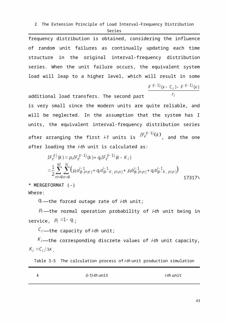
2 The Extension Principle of Load Interval-Frequency Distribution Series
四.2.1 Analysis of Equivalent Interval Frequency Distribution
According to the method described in Section 3.1.1, step length is set as 50MW.
And scanning the net load curve point by point from the beginning, we can get the original
interval-frequency distribution series. For convenience to describe, here the result of each
load interval-frequency distribution series will be restored to the load frequency curve for
analysis. Fig. 4-23 is just the original restored equivalent load frequency curve and the load
frequency curve obtained by FD method, you can see that these two curves are overlapped
completely, indicating that the load interval-frequency distribution series can accurately
restore the load frequency curve, It contains all the information load frequency curve.
0 2000 4000 6000 8000 10000 12000 140000
5
10
15
20
25
30
35
40
x /MW
/向上超越次数次
等效电量频率法本文所提方法
Fig. 4-23 The original load frequency curve
After penetrating the wind power as shown in Fig. 4-23, we can find that the system
minimum load level in the study period 720 hours is 2500MW, the maximum load level is
7500MW. From the whole point of view, the load level ranging from 4000 ~5000MW have a
relatively high transfer frequency and the corresponding units will meet a high frequent
requirement of shutdown and startup, or adjustment of output operations. In the base load
0~2500MW, and the peak load 7000~7500MW, the operating units corresponds to the
smaller load transfer frequency, the relative reduction will happen in the number of
corresponding start and stop operation.
47

2 The Extension Principle of Load Interval-Frequency Distribution Series
Loading units in the Table 4-7 one by one, each equivalent interval-frequency
distribution series is restored into the load frequency curve according to formula (3-10). The
process of convolution is shown in Fig. 4-24 and Fig. 4-25. Among them, the equivalent load
frequency curve in FD method and the proposed method are exactly the same, which can
verify the correctness of the proposed method. At the same time comparing these two
different scenarios, we can find that for the average and maximum load transfer frequency
Scenario 2 is always greater than Scenario 1, which also confirms the degree of timing
fluctuation is increased lot after considering intermittent wind power.
0 2000 4000 6000 8000 10000 12000 14000 160000
5
10
15
20
25
30
35
40
45
50
x /MW
/转移次数次
最终负荷频率曲线
本文所提方法等效电量频率法最终负荷频率曲线。
初始负荷频率曲线中间过程形成的曲线
Fig. 4-24 The detailed convolution process without wind power
48
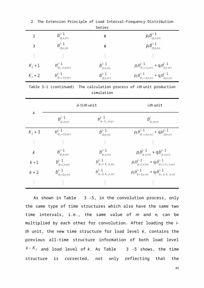
2 The Extension Principle of Load Interval-Frequency Distribution Series
0 2000 4000 6000 8000 10000 12000 14000 160000
5
10
15
20
25
30
35
40
x /MW
/转移次数次
最终负荷频率曲线
初始负荷频率曲线
中间过程形成的曲线 本文所提方法等效电量频率法最终负荷频率曲线。
Fig. 4-25 The detailed convolution process with wind power
Here let’s take the example of the 7-th unit for analysis, whose minimum up time is 7
hours, and minimum down time is 5 hours. And we can find that its loading position is just
the sum of former 6 units capacity, which is equal to 4400MW.
Table 4-8 The equivalent interval-frequency distribution of 4400MW without wind power
49

2 The Extension Principle of Load Interval-Frequency Distribution Series
a(88,1,5)=1.258576
a(88,1,7)=0.419525
a(88,2,4)=0.839050
a(88,14,1)=0.419525
a(88,15,9)=0.419525
a(88,16,8)=0.419525
a(88,16,9)=0.419525
a(88,17,1)=2.936677
a(88,17,4)=0.419525
a(88,17,5)=0.839050
a(88,17,7)=0.646193
a(88,17,10)=0.419525
a(88,18,4)=0.113334
a(88,19,5)=1.103948
a(88,19,6)=0.264898
a(88,19,7)=0.952384
a(88,20,4)=1.829665
a(88,21,4)=0.427179
a(88,22,4)=0.151564
a(88,25,5)=0.419525
a(88,26,4)=0.419525
a(88,69,2)=0.419525
a(88,92,4)=0.113334
a(88,139,4)=0.113334
a(88,139,5)=0.264898
a(88,140,4)=0.151564
a(88,141,1)=0.151564
a(88,143,2)=0.007654
a(88,186,6)=0.113334
a(88,187,4)=0.151564
a(88,213,2)=0.007654
a(88,334,1)=0.007654
b(88,1,1)=1.678101
b(88,1,2)=0.839050
b(88,1,22)=0.151564
b(88,1,25)=0.419525
b(88,1,26)=0.419525
b(88,1,143)=0.007654
b(88,2,21)=0.427179
b(88,2,334)=0.007654
b(88,4,19)=2.056332
b(88,4,20)=1.829665
b(88,4,69)=0.419525
b(88,4,92)=0.113334
b(88,4,139)=0.151564
b(88,4,140)=0.151564
b(88,4,213)=0.007654
b(88,5,17)=3.356202
b(88,5,19)=0.264898
b(88,5,139)=0.113334
b(88,5,141)=0.151564
b(88,6,17)=0.113334
b(88,6,18)=0.113334
b(88,6,187)=0.151564
b(88,7,16)=0.839050
b(88,7,17)=0.952384
b(88,7,139)=0.113334
b(88,7,186)=0.113334
b(88,8,17)=0.419525
b(88,9,14)=0.419525
b(88,9,17)=0.419525
b(88,10,15)=0.419525
Table 4-8 and Table 4-9 give the detailed equivalent interval-frequency distribution
series for the load level 4400MW in two different Scenarios and correspond to spatial
coordinate system, as shown in Fig. 4-26 and Fig. 4-27. We can see clearly that the number
of load transfers of short interval is greatly increased after integrating wind power, and the
load transfer of which the upward duration is more than 7 hours and the corresponding
downward duration is more than 5 hours is increased as well. It indicates that the volatility of
wind power, not only brings more demand of shutdown and startup for generator, but also,
more requests for the generator which cannot be accomplished. We need to eliminate this
part of the short interval fluctuation impact in the dynamic cost evaluation.
50

2 The Extension Principle of Load Interval-Frequency Distribution Series
0 40 80 120 160 200 240 280 320 360 400 440 480 520 560 600 640 680 720
02
46
810
1214
1618
2022
240
0.5
1
1.5
2
2.5
3
/负荷转移频率次
m /h向上转移持续时间n /h向下转移持续时间
Fig. 4-26 The equivalent interval-frequency distribution of 4400MW with and without wind power
51

2 The Extension Principle of Load Interval-Frequency Distribution Series
0 40 80 120 160 200 240 280 320 360 400 440 480 520 560 600 640 680 720
02
46
810
1214
1618
2022
240
0.5
1
1.5
2
2.5
3
3.5
/负荷转移频率次
m /h向上转移持续时间n /h向下转移持续时间
52

2 The Extension Principle of Load Interval-Frequency Distribution Series
Fig. 4-27 The equivalent interval-frequency distribution of 4400MW with and without wind power
53
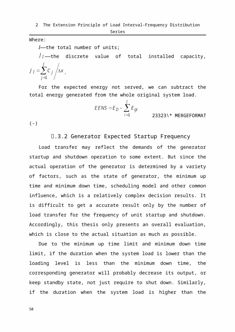
2 The Extension Principle of Load Interval-Frequency Distribution Series
Table 4-9 The equivalent interval-frequency distribution of 4400MW with wind power
a(88,1,1)=0.226667
a(88,1,4)=0.406184
a(88,1,5)=1.72329
a(88,1,7)=0.468124
a(88,2,3)=0.419525
a(88,2,4)=0.166872
a(88,2,6)=0.0409446
a(88,2,12)=0.419525
a(88,3,3)=0.226667
a(88,3,11)=0.419525
a(88,3,21)=0.419525
a(88,4,4)=0.419525
a(88,5,2)=0.151564
a(88,5,3)=0.113334
a(88,6,8)=0.264898
a(88,6,9)=0.532859
a(88,6,13)=0.113334
a(88,7,2)=0.419525
a(88,12,12)=0.419525
a(88,14,1)=0.427179
a(88,14,2)=0.00765421
a(88,14,8)=0.113334
a(88,14,10)=0.151564
a(88,15,8)=0.83905
a(88,15,9)=1.37191
a(88,15,10)=0.113334
a(88,15,11)=0.419525
a(88,16,1)=0.879995
a(88,16,7)=0.722653
a(88,16,8)=0.83905
a(88,19,1)=0.113334
a(88,19,2)=0.141287
a(88,19,5)=1.00231
a(88,20,1)=0.0437099
a(88,20,3)=0.00765421
a(88,20,4)=0.57612
a(88,20,6)=0.151564
a(88,21,1)=0.113334
a(88,21,3)=0.0381682
a(88,21,4)=0.419525
a(88,21,5)=0.0485989
a(88,22,4)=0.00276527
a(88,23,4)=0.113334
a(88,23,8)=0.419525
a(88,23,10)=0.151564
a(88,26,1)=0.00765421
a(88,41,7)=0.113334
a(88,41,10)=0.0076542
a(88,42,6)=0.151564
a(88,43,5)=0.0485989
a(88,44,4)=0.182231
a(88,46,1)=0.151564
a(88,47,5)=0.0409446
a(88,52,1)=0.113334
a(88,63,7)=0.151564
a(88,65,1)=0.0409446
a(88,65,6)=0.00765421
a(88,67,5)=0.0409446
a(88,68,3)=0.00765421
a(88,69,4)=0.141287
b(88,1,1)=2.43838
b(88,2,1)=0.120988
b(88,3,1)=0.151564
b(88,13,1)=0.113334
b(88,1,2)=0.627342
b(88,21,2)=0.419525
b(88,1,3)=0.113334
b(88,2,3)=0.419525
b(88,11,3)=0.113334
b(88,19,3)=0.419525
b(88,8,4)=0.419525
b(88,7,5)=0.113334
b(88,10,5)=0.151564
b(88,2,6)=0.151564
b(88,3,6)=0.226667
b(88,4,6)=0.532859
b(88,9,7)=0.419525
b(88,11,12)=0.419525
b(88,7,14)=0.120988
b(88,10,14)=0.159218
b(88,12,14)=0.419525
b(88,7,15)=0.419525
b(88,8,15)=0.419525
b(88,9,15)=1.37191
b(88,10,15)=0.113334
b(88,12,15)=0.419525
b(88,5,16)=0.571089
b(88,6,16)=0.151564
b(88,7,16)=0.993329
b(88,8,16)=0.990614
b(88,4,19)=0.593355
b(88,5,19)=0.292851
b(88,6,19)=0.00276527
b(88,7,19)=0.141287
b(88,9,19)=0.113334
b(88,1,20)=0.151564
b(88,3,20)=0.0409446
b(88,4,20)=0.578886
b(88,5,20)=0.00765421
b(88,2,21)=0.0409446
b(88,3,21)=0.427179
b(88,4,21)=0.0381682
b(88,9,21)=0.113334
b(88,1,22)=0.00276527
b(88,1,23)=0.684423
b(88,3,26)=0.00765421
b(88,1,41)=0.113334
b(88,4,41)=0.00765421
b(88,7,42)=0.151564
b(88,5,43)=0.0409446
b(88,7,43)=0.00765421
b(88,5,44)=0.182231
b(88,5,46)=0.151564
b(88,1,47)=0.0409446
b(88,1,52)=0.113334
b(88,9,63)=0.151564
b(88,4,65)=0.0409446
b(88,7,65)=0.00765421
b(88,6,67)=0.0409446
b(88,3,68)=0.00765421
54

2 The Extension Principle of Load Interval-Frequency Distribution Series
Table 4-4(continued) The equivalent interval-frequency distribution of 4400MW with wind power
a(88,16,9)=1.10395
a(88,16,10)=0.419525
a(88,16,19)=0.419525
a(88,17,1)=2.40202
a(88,17,4)=0.0409446
a(88,17,7)=2.49847
a(88,17,8)=0.159218
a(88,17,11)=0.113334
a(88,18,2)=0.113334
a(88,18,3)=0.159218
a(88,18,6)=0.0409446
a(88,18,7)=0.347655
a(88,18,8)=0.113334
a(88,69,5)=0.141287
a(88,90,5)=0.151564
a(88,91,4)=0.00765421
a(88,92,3)=0.0409446
a(88,92,4)=0.00276527
a(88,93,1)=0.141287
a(88,115,7)=0.141287
a(88,140,2)=0.0409446
a(88,165,4)=0.141287
a(88,189,6)=0.0027652
a(88,354,4)=0.0027652
a(88,692,4)=0.0381682
a(88,718,2)=0.0460978
b(88,9,16)=0.83905
b(88,10,16)=0.419525
b(88,11,16)=0.419525
b(88,3,17)=0.113334
b(88,4,17)=0.419525
b(88,5,17)=1.49365
b(88,6,17)=0.200163
b(88,7,17)=2.18191
b(88,8,17)=0.805411
b(88,1,18)=0.120988
b(88,4,18)=0.120988
b(88,5,18)=0.264898
b(88,7,18)=0.154278
b(88,8,18)=0.113334
b(88,1,19)=0.113334
b(88,1,69)=0.141287
b(88,5,69)=0.141287
b(88,7,90)=0.151564
b(88,5,91)=0.00765421
b(88,4,92)=0.00276527
b(88,5,92)=0.0409446
b(88,4,93)=0.141287
b(88,4,115)=0.141287
b(88,4,140)=0.0409446
b(88,2,165)=0.141287
b(88,4,189)=0.0027652
b(88,5,354)=0.0027652
b(88,3,692)=0.0381682
b(88,2,718)=0.0460978
According to the formula (3-8) and (3-13), select the satisfied time structure to calculate
the frequency of startup and shutdown frequency and we can obtain the following Table 4-
10. Comparing these two different scenarios, the total upward and downward transfer are
both increased approximately by 60% and for the first type of time structure of short interval
is increased by 26.8%, the second type is 31.9%.
Table 4-10 The statistics of equivalent time structure of 4400MW
ScenarioDownward transfer
Short time interval
Expected shutdown frequency
Upward transfer
Short time interval
Expected startup
frequency
Scenario 1
14.66 9.13 5.53 14.66 7.65 7.01
scenario 2
23.47 12.03 11.43 23. 47 9.70 13.77
55
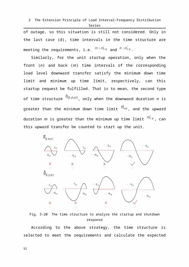
2 The Extension Principle of Load Interval-Frequency Distribution Series
At the same time we can also find that here is about more than 50% belonging to the
short time interval in both kinds of time structures, which is not in accordance with the
requirements of the appropriate unit startup and shutdown. If this kind of time structure is
eliminated, it will introduce significant errors during dynamic cost evaluation.
四.2.2 Analysis of Probabilistic Production Simulation
Table 4-11 The comparison of unit expected energy with wind power
Unit
Expected energy of i-th unit
(MW·h) Unit
Expected energy of i-th unit
(MW·h)Proposed method
EEF method Proposed method EEF method
1 749952 749952 19 3009.73 3104.552 749952 749952 20 2848.59 2947.213 363032 363426 21 2707.75 2784.814 343412 344736 22 2547.68 2633.265 221050 222224 23 2405.93 2489.176 202051 203442 24 2275.18 2354.677 182622 184087 25 2154.04 2221.978 87955 88756.6 26 2026.48 2095.649 82713.5 83429.6 27 1904.75 1973.910 77259.5 78031.8 28 1790.6 1858.3511 71347.9 72251.5 29 1686.22 1746.9812 193811 197078 30 1583.82 1641.1213 118737 121345 31 1485.13 1540.6514 23446.9 24042.4 32 1392.07 1445.9615 19358.9 19891.2 33 1305.74 1355.6616 15865 16318.4 34 1222.69 1269.3617 3375.21 3450.34 35 1142.54 1187.17
18 3160.58 3278.26 36 1066.83 1109.8
Table 4-12 The comparison of reliability index with wind power
Index Proposed method EEF method
Original system load [104MW·h] 351.35 353.16
EENS [104MW·h] 1.3192 1.3796
LOLP 0.0337 0.0341
Table 4-11 and Table 4-12 give the result of expected energy of each unit and reliability
56

2 The Extension Principle of Load Interval-Frequency Distribution Series
index with wind power in EEF method and proposed method. Not difficult to find, the
desirable energy for each unit is similar to each other and the reliability index is similar as
well, which can verify the correctness of the proposed method in generating energy and
reliability assessment.
四.3 Assessment of Dynamic Costs
四.3.1 Analysis of Generator Expected Startup and Shutdown Frequency
For the expected startup and shutdown frequency of units, this thesis employs the FD
method and proposed method for comparison. In the proposed algorithm, it is also calculated
in case of no elimination. The detailed results are given in Table 4-13. First of all, we can
find that the startup and shutdown frequency in the proposed method is decreased
respectively, 30.2%, 34.6% compared with the one in FD method after removing the time
structure of short time interval. In the other words, the eliminated time structures is taking up
almost one third in the total distribution. If it includes the time structures of short time
interval, the result is fully consistent with the one in FD method, which can demonstrate the
validity of the proposed algorithm once again.
Table 4-13 The expected startup frequency of each unit
UnitProposed method
FD methodInclude short time interval Exclude short time interval
1 0 0 02 0 0 03 0 0 04 1.08 3.24 3.245 6.06 12.94 12.946 9.79 20.22 20.227 13.77 23.47 23.478 19.68 27.54 27.549 19.9 26.5 26.510 20.78 27.72 27.7211 20.55 26.73 26.7312 15.14 24.99 24.9913 10.79 20.93 20.9314 8.69 16.7 16.715 7.48 14.37 14.37
57

2 The Extension Principle of Load Interval-Frequency Distribution Series
16 6.13 12.27 12.2717 8.55 10.04 10.04
Table 4-8(continued) The expected startup frequency of each unit
UnitProposed method
FD methodInclude short time interval Exclude short time interval
18 8.31 9.82 9.8219 7.99 9.29 9.2920 7.69297 8.91397 8.9139723 6.57 7.78 7.7824 6.3 7.37 7.3725 5.98 7.01 7.0126 5.65 6.71 6.7127 5.36 6.38 6.3828 5.12 6.06 6.0629 4.85 5.74 5.7430 4.57 5.46 5.4631 4.32 5.18 5.1832 4.09 4.91 4.9133 3.88 4.63 4.6334 3.65 4.38 4.3835 3.42 4.13 4.13
36 3.22 3.89 3.89
Table 4-14 The expected shutdown frequency of each unit
UnitProposed method
FD methodInclude short time interval Exclude short time interval
1 0 0 02 0 0 03 0 0 04 1.08 3.24 3.245 5.11 12.94 12.946 7.81 20.22 20.227 11.43 23.47 23.478 16.46 27.54 27.549 18.24 26.50 26.5010 18.96 27.72 27.7211 18.80 26.73 26.7312 14.23 24.99 24.9913 10.32 20.93 20.9314 7.93 16.70 16.7015 6.82 14.37 14.37
58

2 The Extension Principle of Load Interval-Frequency Distribution Series
16 5.64 12.27 12.27
17 8.55 10.04 10.04
Table 4-9(continued) The expected shutdown frequency of each unit
UnitProposed method
FD methodInclude short time interval Exclude short time interval
18 8.31 9.82 9.8219 7.99 9.29 9.2920 7.69 8.91 8.9121 7.24 8.52 8.5222 6.88 8.18 8.1823 6.57 7.78 7.7824 6.3 7.37 7.3725 5.98 7.01 7.0126 5.65 6.71 6.7127 5.36 6.38 6.3828 5.12 6.06 6.0629 4.85 5.74 5.7430 4.57 5.45 5.4531 4.32 5.18 5.1832 4.09 4.91 4.9133 3.88 4.63 4.6334 3.65 4.38 4.3835 3.42 4.13 4.1336 3.22 3.89 3.89
四.3.2 Analysis of Dynamic Costs
Table 4-15 The comparison of each dynamic cost index
Dynamic cost indexProposed method
FD methodInclude short time
intervalInclude short time
interval
12.94 22.37 22.37
[105$] 5.56 8.17 8.17
[106$] 1.13 1.65 2.59
[105$] 5.03 8.17 8.17
[105$] 21.85 32.83 42.28
59
2 The Extension Principle of Load Interval-Frequency Distribution Series
Table 4-15 gives the specific dynamic costs of each index. Due to the exclusion of the
time structure of short interval, the final dynamic costs in the proposed method, is decreased
by 48.2% compared with the one in FD method. In the case of no elimination in proposed
method, each index is exactly the same with the one in FD method, except for the boiler
startup cost, since the offline time for each startup is directly the average in FD method,
while in proposed method, it is the corresponding downward duration for the exact offline
time. It can also show the correctness of this proposed method.
In order to evaluate the impact of short term fluctuations in the time structure, the Short
Time Interval Dynamic Cost is induced and the result is as follows.
35335\*MERGEFORMAT (-)
Eliminating these time structures of short interval, will result in the factor that it needs
to keep some units in the state of standby, which will have an economic effect to some
extent. Here the Short Time Interval Proportion of Unit Capacity is induced to
reflect this part influence from the point of view of the proportion of the total time and
calculated as follows.
36336\*MERGEFORMAT (-)
Table 4-16 Probabilistic production simulation results based on interval-frequency distribution
60

2 The Extension Principle of Load Interval-Frequency Distribution Series
Production cost Scenario 1 Scenario 2
Original system load [104MW·h] 399.32 351.35
EENS [104MW·h] 3.0035 1.3192
LOLP 0.0727 0.0337
Dynamic cost [106$] 2.07 2.18
Fuel cost c [106$] 2.22 1.80
Environmental cost [107$] 2.51 2.19
Customer interruption cost [107$] 3.00 1.32
Total cost [107$] 5.95 3.91
Table 4-16 shows the probabilistic production simulation results in different scenarios.
With the wind power, the EENS is decreased by 56% and LOLP is reduced by 53.66%,
indicating that wind power will help to improve the reliability of original power system. For
the fuel cost, it saves by 18.9% and the environmental cost is decreased by 12.8%, the
customer interruption cost is also reduced 56%. Meanwhile, the preventable costs of wind
power is $, the total production cost saves by 34.3% with wind power.
四.3.3 The Influence of Wind Capacity
To further investigate how the wind power capacity affects the results, we compare the
evaluation in different penetration scenarios of wind power ranging from 0~1500MW,
especially for the short time interval dynamic cost , short time interval proportion of
unit capacity and the dynamic cost rate .
37337\* MERGEFORMAT (-)Where:
——dynamic cost in the proposed method;——the total production cost.
The relationship between the dynamic cost index and the number of wind turbines is
shown in Fig. 4-28 and Fig. 4-29. It can be seen, both the short interval dynamic cost and
short time interval proportion of unit capacity trend to grow with the increasing amount of
61

2 The Extension Principle of Load Interval-Frequency Distribution Series
wind power integration, which is consistent with the increased volatility and with the
increased effect caused by the short time interval fluctuations.
At the same time, there is a partial decline phenomenon of the dynamic cost with the
increasing wind power integration. This is mainly because the loading position of each unit
is changed by the different of volatility of wind power. The corresponding required unit
shutdown and startup will also change since the strongest fluctuated load interval varies with
different penetration of wind power.
0 300 600 900 1200 1500
0.3
0.32
0.34
0.36
0.38
0.4
0.42
0.44
0.46
/MW风电装机容量
短时间间隔动态费用
Fig. 4-28 The relationship between short interval dynamic cost and the number of wind turbines
62

2 The Extension Principle of Load Interval-Frequency Distribution Series
0 300 600 900 1200 15006
7
8
9
10
11
12
13
/MW风电装机容量
机组单位容量短时间间隔时长比例
Fig. 4-29 The relationship between short time interval proportion of unit capacity
and the number of wind turbines
As shown in Fig. 4-30, the dynamic cost rate is only 3.64%without any wind power.
When it is penetrated 700MW of wind power, the dynamic cost rate is growing into 5.17%;
and when the wind farm installed capacity is increased to 1500MW, the dynamic cost rate
will become as high as 6.1%. Obviously, with increasing wind power installed capacity,
dynamic cost rate will be gradually increased. Hence to some extent, during the wind farm
planning, we can take advantage of this proposed algorithm to determine the appropriate
scale of penetrated wind power based on the expected dynamic cost rate.
63

2 The Extension Principle of Load Interval-Frequency Distribution Series
0 300 600 900 1200 15003.5
4
4.5
5
5.5
6
6.5
/MW风电装机容量
/%动态费用率
Fig. 4-30 The relationship between dynamic cost rate and the number of wind turbines
0 2 4 6 8 10 12 14 163
3.5
4
4.5
5
5.5
6x 10
7
Fig. 4-31 The relationship between generating cost and the number of wind turbines
64

2 The Extension Principle of Load Interval-Frequency Distribution Series
五 Conclusions
With the increasing penetration of wind power into the grid, probabilistic production
simulation with the coexistence of multiple energy intermittent is playing an important role
in the plan and operation, reliability assessment and spare capacity determination of power
system. Therefore, it is significantly meaningful in the wind power grid integration to study
and discuss about the probability production simulation including wind farms. Generally
speaking, the traditional methods, neglect the timing fluctuation of system load, resulting in
the fact that it fails to include the dynamic costs related to the minimum up-time time or
minimum down-time time limits, ramping rate restriction, generator scheduling, and other
factors in the production simulation process. The final production cost is relatively sketchy.
With the growing amounts of the intermittent energy, such as wind power, the volatility of
power system is further improved, the unit shutdown and startup operation is becoming more
frequently and the dynamic cost is also increased a lot. This thesis extends the load
frequency curve into the interval frequency distribution series which contains both the load
fluctuation frequency information and timing distribution information. Based on this series, a
new kind of method has been developed to evaluate the frequency of startup and shutdown
operation and get a more reasonable assessment of dynamic costs, which can be better
applied to a comprehensive assessment of the power system production costs. The main
research achievement can be summarized as the following three points.
(1) First of all, aiming at describe the load timing volatility, the interval-frequency
distribution series is expanded based on load transfer from the load frequency curve. Not
only it can reflect the fluctuation frequency information, but also it can record the timing
distribution of each load transfer in the form of time structure. Meanwhile, this kind of series
can be completely accurately restore to the corresponding load frequency curve. there exists
a certain reference value in characterizing the timing characteristics of the system load.
(2) Analog to the traditional probabilistic production simulation, we employ the
standard convolution to consider the unit random failure as the modification of each time
structure in the original interval-frequency distribution series. In this way, both the
fluctuation frequency information and timing distribution can be taken into account in the
simulation process. Then based on the detailed information inside the structure in the
65

2 The Extension Principle of Load Interval-Frequency Distribution Series
equivalent distribution series, the expected energy of each power generating units and
reliability analysis is evaluated, and compared with the classical equivalent energy function
method, the difference is not that big, which demonstrates its validity from this point of
view.
(3) For the evaluation of dynamic cost, it is assumed that the request of unit shutdown
due to load downward transfer will be fulfilled only when its adjacent two time intervals are
larger than the minimum up time and minimum down time limits, respectively. Similarly, the
request of unit startup due to load upward transfer will be fulfilled only when its adjacent
two time intervals are larger than the minimum down time and minimum up time limits.
With this assumption to consider the infeasibility of startup and shutdown in a short time
interval, we can get a more rational assessment for the unit shutdown and startup frequency,
compared with the one in frequency and duration method. The related dynamic cost is more
close to the actual system conditions.
With the increasing penetration of wind power, more impact will be produced by the
growing volatility. The proportion of short time interval in the interval frequency distribution
series is increasing dramatically, affecting the assessment dynamic costs a lot. It’s worthy to
be considered in the simulation process The proposed method can be combined with other
applications to apply for the comprehensive evaluation of production costing and the effect
of wind farm installed capacity.
66
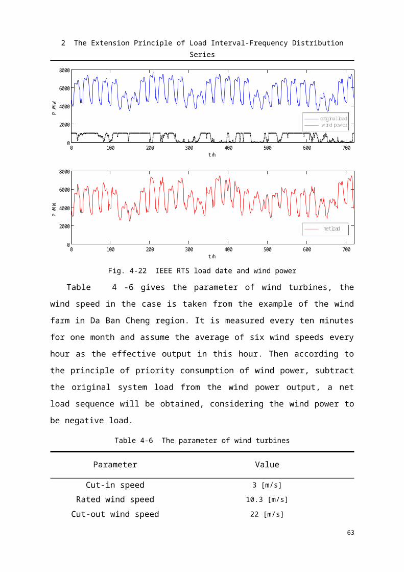
References
References
[1] Wang Xifan. Power system optimization planning[M]. China Hydraulic Engineering Press, 1990.[2] Liu Zhenya. China Electric Power and Energy[M]. China Electric Power Press, 2012.[3] Zhoutian Rui, Wang Xu, Zhang Qian, et al. Analysis of related problems with a large scale wind
farm penetration in Jilin Province[J]. Journal of China Electric Power, 2008, 36 (3): 1-3,8.[4] Zhoutian Rui, Wang Xu, Zhang Qian, et al. Empirical Analysis of the influence of planning large-
scale wind power in Jiangsu Power Grid [J]. Journal of China Electric Power, 2010, 43 (2): 11-15.[5] The grid technology (training) center of Northwest Power Grid Co., Ltd., the Wind Power Research
Center of Northwest Power Grid Co., Ltd.. Northwest (Jiuquan) wind power output characteristics[R]. Northwest Power Grid Co., Ltd., 2008.
[6] China Electricity Enterprise Council. China Power Industry Status and Prospects[OL]. http://www.cec.org.cn/yaowenkuaidi/2015-03-10/134972.html.
[7] Wei Xianfei. The current status and prospect of wind power development. Journal of Business Economics, 2010,364 (12): 21-23.
[8] Xiao Chong Ying, Wang Ning Bo, Ding Kun, Zhi Jing. Gansu Jiuquan wind power adjustment mode [J]. Proceedings of the CSEE, 2010,30 (10): 1-7.
[9] Xiao Chong Ying, Wang Ning Bo, Zhi Jing, Ding Kun. Jiuquan wind power output characteristic analysis [J]. Journal of Electric Power System and its Automation, 2010,17: 64-67.
[10] Zhang Ning, Zhou Tianrui, Duan Changgang, and so on. The impact of large-scale wind farms on the power system peaking regulation [J]. Journal of Power System Technology, 2010,34 (1): 152-158.
[11] Sun Rongfu, Zhang Tao, Liang Ji. Assessment and application of wind power capacity acceptance [J]. Journal of electric power system and its automation, 2011 (4): 70-76.
[12] Han Xiaoqi, Sun Shouguang, Qiqing Ru. Assessment from the system point of view grid peaking acceptance of wind power capacity [J]. Journal of China Electric Power, 2010,43 (6): 16-19.
[13] Xinjiang Electric Power Company. Preliminary analysis of the impact of Da Bancheng wind power in Urumqi power grid operation [J]. Journal of China Wind power, 998, (3): 23-25.
[14] Liu Hong. A preliminary study proportion of allowed wind power in Urumqi grid[J]. Journal of China Wind power, 1999, (15): 28-29.
[15] Booth R R. Power system simulation model based on probability analysis[J]. IEEE Transactions on 91.1(1972):62-69.
[16] Billinton R, Li W. A Monte Carlo method for multi-area generation system reliability assessment[J]. IEEE Transactions on Power Systems,1992,7(4):1487-1492.
[17] Stremel J, Jenkins R, Babb R, et al. Production costing using the cumulant method of representing the equivalent load curve[J]. IEEE Transactions on Power Apparatus and Systems, 1980, 5(PAS-99): 1947-1956.
[18] Rau N S, Toy P, Schenk K F. Expected energy production costs by the method of moments[J]. Power Apparatus and Systems, IEEE Transactions on, 1980 (5): 1908-1917.
[19] Wang Xifan. Fundamental of Power system optimization planning[M]. China Electric Power Press, 1994: 64-95.
[20] Wang Xifan. EEF approach to power system probabilistic modeling [J]. Journal of Xi’an Jiaotong University, 1984, 18(6): 13-26.
67

Research Achievements during the study
[21] Wang X. Equivalent energy function approach to power system probabilistic modeling[J]. IEEE Transactions on Power Systems,1988,3(3):823-829.
[22] Xia Qing, Wang Shaojun, Xiang Niande. The probabilistic power system production simulation based on chronological load curve [J]. Proceedings of the CSEE, 1994, 14(3): 21-28.
[23] Xia Qing, Wang Shaojun, Xiang Niande. The probabilistic power system production simulation based on chronological load curve [J]. Proceedings of the CSEE, 1998, 18(6): 429-433.
[24] Liao Yuhan. Probabilistic production simulation with wind farms and application [D]. North China Electric Power University, 2012.
[25] Shi Wenhui, Chen Jing, Wang Weisheng. Reliability Assessment of interconnected power system with wind farms [J]. Journal of Power System Technology, 2012,36 (2): 224-230.
[26] Liu Xu. Stochastic production costing with wind farms [D]. Shandong University, 2013.[27] Wang Xifan, Wang Xiuli. Probabilistic production simulation method and its application[J]. Journal
of Electric Power System and its Automation,, 2003, 27(8): 10-15. [28] Zou Bin, Li Dong. Power system probabilistic production simulation with wind generation based on
available capacity distribution[J]. Proceedings of the CSEE, 2012, 32(7): 23-31. [29] Zhang Ning, Kang Chongqing, Chih Chen Ping, et al. Wind power trusted capacity calculation
method based on computing sequence [J]. Proceedings of the CSEE, 2011,31 (25): 1-9.[30] Hu Guowei, Bie Zhaohong, Wang Xifan. Optimal dispatch in wind integrated system considering
operation reliability[J]. Transactions of China Electrotechnical Society, 2013, 28(5): 58-65. [31] Chen Shuyong, Dai Huizhu. Stochastic production costing with wind farms [J]. Journal of China
Electric Power, 2000,33 (3): 30-31.[32] Zhang Ningyu, Gao Shan, Zhao Xin. An unit commitment model and algorithm with randomness of
wind power[J]. Transactions of China Electrotechnical Society, 2013, 28(5): 22-29. [33] Grubb, Michael. The inclusion of dynamic factors in statistical power system cost models. I.
Assessment of startup and banking costs[J]. Power Systems, IEEE Transactions on 4.2 (1989): 419-425.
[34] Grubb, Michael. The inclusion of dynamic factors in statistical power system cost models. II. Part loading and reserve costs[J]. Power Systems, IEEE Transactions on 4.2 (1989): 524-529.
[35] Arif S. Malik, Brian J. Cory. An application of frequency and duration approach in generation planning[J]. Power Systems, IEEE Transactions on 12.3 (1997): 1076-1084.
[36] Malik, A. S. Simulating limited energy units within the framework of ELDC and FD methods[J]. International journal of electrical power & energy systems 26.8 (2004): 645-653.
[37] Zhang Jietan, Cheng Haozhong, Hu Zechun, et al. Power system probabilistic production simulation including wind farms[J]. Proceedings of the CSEE, 2009, 29(28): 34-39.
[38] Qu Chong, Wang Xiuli, Xie Shaoyu, et al. Improved algorithm for probabilistic production simulation of power systems with wind power[J]. Journal of Xi’an Jiaotong University, 2012, 46(6).
[39] Yuan Jiandang, Yuan Tiejiang, Chao Qin, Li Yiyan. Study of generation expansion planning of the power system incorporating large-scale wind power in the environment of electricity market[J]. Power System Protection and Control, 2013, 28(5): 22-29.
[40] Lei Yazhou, Wang Weisheng, Yin Yonghua, et al. Analysis of wind power value to power system operation[J]. Power System Technology, 2002, 26(5): 10-14.
[41] Liu Jin, Yu Jilai, Liu Zhuo. An intelligent optimal dispatch strategy for spinning reserve coping with wind intermittent disturbance[J]. Proceedings of the CSEE, 2013, 33(1): 163-170.
[42] Tuoh Y. A., Meibom P., Denny E., et al. Unit commitment for systems with significant wind penetration[J]. IEEE trans on power systems, 2009, 24(2): 592-60.
[43] Nakamura S.. A review of electric production simulation and capacity expansion planning programs[J], Energy research, Vol. 8,231-240, 1984.
68

References
[44] Palsson M., Uhlen K,T. Oftevaag T et al. Large-scale wind power integration and voltage stability limits in regional networks[C]. IEEE power engineering society summer meeting, Chicago, USA, 2000: 762-769.
[45] Wiik J., Gjengedal T.,Gjerde J.O., et al. Steady state Power system issues when Planning large wind farms[C]. IEEE power engineering society winter meeting, 2004,1: 199-204.
[46] Amora M. A. B.,Bezerra U. H.. Assessment of the effects of wind farms connected in a power system[C]. Power tech proceedings, 2011 IEEE porto.,4: 6.
[47] Tande J. 0.G., Uhlen K.. Wind turbines in weak grids-constraints and solutions[C]. 16th international conference and exhibition on electricity distribution part 1: contributions and summaries, 2006: 261.
[48] The Reliability Test System Task Force of the Application of Probability Methods Subcommittee. IEEE Reliability Test System [J]. IEEE Transactions on Power Apparatus and Systems, 1979, 98(6) : 2047-2054.
[49] Hall, J. D., R. J. Ringlee, and A. J. Wood. Frequency and duration methods for power system reliability calculations: I-Generation system model[J]. Power Apparatus and Systems, IEEE Transactions on 9 (1968): 1787-1796.
[50] Ringlee, Robert J., and Allen J. Wood. Frequency and duration methods for power system reliability calculations: II-Demand model and capacity reserve model[J]. Power Apparatus and Systems, IEEE Transactions on 4 (1969): 375-388.
[51] Galloway, CHARLES D., et al. Frequency and Duration Methods for Power System Reliability Calculations Part III: Generation System Planning[J]. Power Apparatus and Systems, IEEE Transactions on 8 (1969): 1216-1223.
[52] Ringlee, Robert J., and Allen J. Wood. Frequency and Duration Methods for Power System Reliability Calculations, Part V: Models for Delays in Unit Installations and Two Interconnected Systems[J]. Power Apparatus and Systems, IEEE Transactions on 1 (1971): 79-88.
[53] Hasche, B. Keane, A,O'Malley, M. Capacity Value of Wind Power, Calculation, and Data Requirements: the Irish Power System Case[J]. IEEE Transactions on Power Systems, 2011,26(1): 420-430.
[54] Dobakhshari A S, Fotuhi-Firuzabad M. A reliability model of large wind farms for power system adequacy studies[J]. IEEE Transactions on Energy Conversion, 2009, 24(3): 792-801.
[55] Xie Kaigui. Considering wind speed correlation of WECS in reliability evaluation using the time-shifting[J]. Electric Power system Research, 2009, 79(4): 687-693.
[56] Ning Zhang, Chongqing Kang, et al. Simulationmethodology of multiple wind farms operation considering wind speedcorrelation[J]. International Journal of Power and Energry System, 2010, 4(30): 264-27.
69

Research Achievements during the study
Research Achievements during the study
[1] 金烂聚,王秀丽,等.高压直流输电谐波保护综述[C].中国高等学校电力系统及其自动化专业第三十届学术年会.北京:北京交通大学,2014.
[2] Linhong, Xie, Lanju Jin, Xiuli Wang, et al. Improved Protection Method of HVDC Transmission Line Based on the Analysis of Traveling Wave Dispersion [C]. CSEE and IEEE PES International Conference on Power System Technology. Chengdu, China on October, 2014:467~473 (DOI: 10.1109/POWERCON.2014.6993712).
[3] Lanju Jin, Xiuli Wang, et al. Power System Probabilistic Production Simulation Based on Equivalent Interval Frequency Distribution Including Wind Farms[C]. CSEE and IEEE PES International Conference on Power System Technology. Chengdu, China on October, 2014:336~342 (DOI: 10.1109/POWERCON.2014.6993631).
[4] Lanju Jin, Wenhui Shi, et al. An improved algorithm for Power System Probabilistic Production Simulation Based on Equivalent Interval Frequency Distribution[C]. IEEE PES Asia-Pacific Power and Energy Engineering Conference. Hong Kong, China on December, 2014:1~4 (DOI:10.1109/APPEEC.2014.7066154).
70