CS/ECE/ISyE 524 Introduction to Optimization Spring 2017–18

21. Set cover and TSP

� Set covering

� Cutting problems and column generation

� Traveling salesman problem

Laurent Lessard (www.laurentlessard.com)

Set covering

� We are given a set of objects M = {1, 2, . . . ,m}.

� We are also given a set S of subsets of M . Example:

I M = {1, 2, 3, 4, 5, 6}I S = {{1, 2}, {1, 3, 5}, {1, 2, 4, 5}, {4, 5}, {3, 6}}

� The problem is to choose a set of subsets (from S) so thatall of the members of M are covered.

� The set C = {{1, 2}, {1, 2, 4, 5}, {3, 6}} is a cover.

� We may be interested in finding a cover of minimum cost.Example: minimize the number of subsets used.

� Let xi = 1 if the i th member of S is used in the cover.

21-2

Formulation (of previous example)

Reminder: S = {{1, 2}, {1, 3, 5}, {1, 2, 4, 5}, {4, 5}, {3, 6}}

minimize x1 + x2 + x3 + x4 + x5

subject to

x1 + x2 + x3 ≥ 1x1 + x3 ≥ 1

x2 + x5 ≥ 1x3 + x4 ≥ 1

x2 + x3 + x4 ≥ 1x5 ≥ 1

xj ∈ {0, 1} ∀j

21-3

More set covering: Kilroy county

� There are 6 cities in Kilroy County.

� The county must determine where to build fire stations toserve these cities. They want to build the stations in someof the cities, and to build the minimum number of stationsneeded to ensure that at least one station is within 15minutes driving time of each city.

� Can we formulate an integer program whose solution givesthe minimum number of fire stations and their locations?

21-4

Driving distances

1 2 3 4 5 6

1 0 10 20 30 30 202 10 0 25 35 20 103 20 25 0 15 30 204 30 35 15 0 15 255 30 20 30 15 0 126 20 10 20 25 12 0

Model

� set of cities: M = {1, 2, 3, 4, 5, 6}� xj = 1 if we build a fire station in city j

� cities within 15 minutes of each city:S = {{1, 2}, {1, 2, 6}, {3, 4}, {3, 4, 5}, {4, 5, 6}, {2, 5, 6}}

21-5

Kilroy county model

S = {{1, 2}, {1, 2, 6}, {3, 4}, {3, 4, 5}, {4, 5, 6}, {2, 5, 6}}

minimizex

x1 + x2 + x3 + x4 + x5 + x6

subject to:

1 1 0 0 0 01 1 0 0 0 10 0 1 1 0 00 0 1 1 1 00 0 0 1 1 10 1 0 0 1 1

x1x2x3x4x5x6

≥

111111

xi ∈ {0, 1} ∀i

� Optimal solution: x2 = x4 = 1 (two fire stations)

21-6

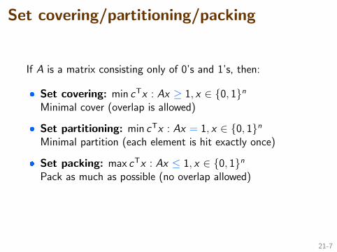
Set covering/partitioning/packing

If A is a matrix consisting only of 0’s and 1’s, then:

� Set covering: min cTx : Ax ≥ 1, x ∈ {0, 1}nMinimal cover (overlap is allowed)

� Set partitioning: min cTx : Ax = 1, x ∈ {0, 1}nMinimal partition (each element is hit exactly once)

� Set packing: max cTx : Ax ≤ 1, x ∈ {0, 1}nPack as much as possible (no overlap allowed)

21-7

Cutting problem

A sheet metal workshop has received the following order:

Dimensions 36× 50 24× 36 20× 60 18× 30

Quantity 8 13 5 15

Theses pieces of sheet metal need to be cut from stock sheets,which measure 48× 96. How can this order by satisfied byusing the least number of large sheets?

� There are relatively few ways to cut a large sheet intosmaller sheets.

� Enumerate all the possibilities!This is called column generation.

21-8

Cutting problem

� This enumeration can be tedious, but the problem is easyto solve once we have figured it out.

21-9

Cutting problemSummary of demands: (vector b)

Dimensions 36× 50 24× 36 20× 60 18× 30

Quantity 8 13 5 15

Summary of possible patterns, each is a column: (matrix A)

Pattern 1 2 3 4 5 6 7 8 9 10 11 12 13 14 15 16

36× 50 1 1 1 0 0 0 0 0 0 0 0 0 0 0 0 024× 36 2 1 0 2 1 0 3 2 1 0 5 4 3 2 1 020× 60 0 0 0 2 2 2 1 1 1 1 0 0 0 0 0 018× 30 0 1 3 0 1 3 0 2 3 5 0 1 3 5 6 8

� xj is the number of times we use pattern j (integer).

� set covering problem where each pattern can be reused.

21-10

Model for cutting problem

minimize x1 + · · ·+ x16

subject to: Ax ≥ b

xi ∈ Z+

� Not a feasible method if we have many (100s) of patterns.

� If we use fewer columns (fewer patterns), the solution willstill be an upper bound on the optimal one.

� This approach is also useful for problems such as flightcrew scheduling: list the possible crew pairings with theirassociated costs, and solve the set cover problem.

21-11

Another cutting example

A plumber stocks standard lengths of pipe, all of length 19 m.An order arrives for:

� 12 lengths of 4m

� 15 lengths of 5m

� 22 lengths of 6m

How should these lengths be cut from standard stock pipes soas to minimize the number of standard pipes used?

� some similarity to a knapsack problem

� how should we model this?

21-12

Another cutting example

One possible model:

� Let N be an upper bound on the number of standard pipes.One possible upper bound is N = 16 (3 pipes per standard).

� Let zj = 1 if we end up cutting standard pipe j .

� Let xij = number of pipes of length i to cut from pipe j .

� If xij > 0 then zj = 1 (fixed cost).

� Obvious upper bounds: x1j ≤ 4, x2j ≤ 3, and x3j ≤ 3.

21-13

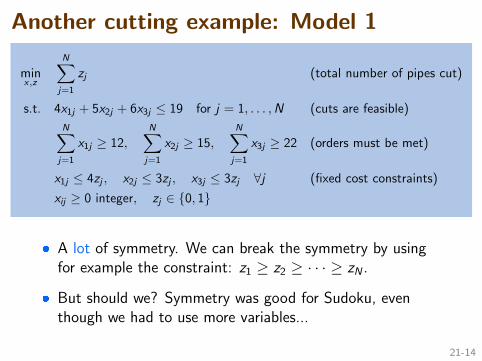
Another cutting example: Model 1

minx,z

N∑j=1

zj (total number of pipes cut)

s.t. 4x1j + 5x2j + 6x3j ≤ 19 for j = 1, . . . ,N (cuts are feasible)

N∑j=1

x1j ≥ 12,N∑j=1

x2j ≥ 15,N∑j=1

x3j ≥ 22 (orders must be met)

x1j ≤ 4zj , x2j ≤ 3zj , x3j ≤ 3zj ∀j (fixed cost constraints)

xij ≥ 0 integer, zj ∈ {0, 1}

� A lot of symmetry. We can break the symmetry by usingfor example the constraint: z1 ≥ z2 ≥ · · · ≥ zN .

� But should we? Symmetry was good for Sudoku, eventhough we had to use more variables...

21-14

Implementation of Model 1

IJulia code: CuttingPipe.ipynb

Solver comparison:

Cbc solver Gurobi solver

standard formulation 0.05 sec 0.02 sec

with symmetry broken 0.02 sec 0.0055 sec

Using 10 times more demand:

Cbc solver Gurobi solver

standard formulation 0.6 sec 3.3 sec

with symmetry broken 6.5 sec 19 sec

I give up...

21-15

Moving forward

Downsides of the first model:

� very large space with a lot of redundancy

� solve time scales poorly with problem size

� (scaling the demand should just scale the solution!)

Observations:

� The optimal solution will consist of patterns, such as(5 + 6 + 6) or (4 + 4 + 5 + 6).

� Even if there are many possible patterns, the optimalsolution will only use a few different ones.

� Can we take advantage of these facts?

21-16

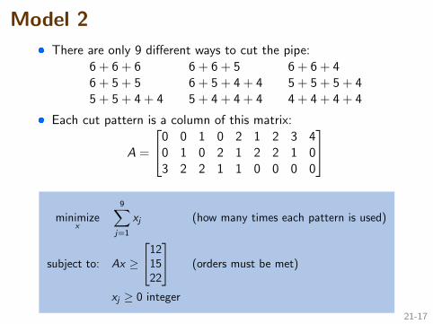
Model 2

� There are only 9 different ways to cut the pipe:

6 + 6 + 6 6 + 6 + 5 6 + 6 + 46 + 5 + 5 6 + 5 + 4 + 4 5 + 5 + 5 + 45 + 5 + 4 + 4 5 + 4 + 4 + 4 4 + 4 + 4 + 4

� Each cut pattern is a column of this matrix:

A =

0 0 1 0 2 1 2 3 40 1 0 2 1 2 2 1 03 2 2 1 1 0 0 0 0

minimizex

9∑j=1

xj (how many times each pattern is used)

subject to: Ax ≥

121522

(orders must be met)

xj ≥ 0 integer

21-17

Implementation of Model 2

IJulia code: CuttingPipe.ipynb

Solver comparison:

Cbc solver Gurobi solver

original problem 0.003 sec 0.003 sec

scaled by 10 0.003 sec 0.003 sec

scaled by 100 0.003 sec 0.003 sec

scaled by 1,000 0.003 sec 0.003 sec

scaled by 1,000,000 0.003 sec 0.003 sec

Much better!

21-18

Larger instances

� If we had much larger pieces of standard pipe, there wouldbe a very large number of possible patterns.

� No longer feasible to enumerate them all

� We shouldn’t have to! Each column represents a potentialvertex. Most will lie inside the feasible polyhedron.

� Column generation strategy:

I Pick a small number of columns to start

I Solve the LP relaxation

I Use the dual to help pick a new column

I Add the column to the A matrix and repeat

21-19

Column generation

1. Start with columns A =[a1, . . . , ak

]2. Solve MIP: minimize

∑i xi subject to Ax ≥ b.

3. Obtain dual variable λ? to the Ax ≥ b constraint.

4. If we add a new column a, cost will drop by aTλ?.

I Suppose aT =[p q r

]Tis the new column.

I Solve MIP: maximize aTλ? subject to 4p + 5q + 6r ≤ 19.

I Add new column to A: ak+1 = a?.

5. Repeat from step 2.

Column generation can be an effective strategy when it’simpossible to enumerate all possible columns. Only columnsthat are deemed likely to help reduce the cost are added.

21-20

Traveling salesman

A traveling salesman must visit a set of cities N and incur aminimal total cost. The salesman starts and ends at home.

� cij is the cost of traveling from city i to city j .

� This is perhaps the most famous combinatorialoptimization problem. There are lots of applications!

� Obvious choice of decision variables:

xij =

{1 we travel from city i to city j

0 otherwise

21-21

Possible TSP model

minimizex

∑i∈N

∑j∈N

cijxij

subject to:∑i∈N

xij = 1 ∀j (one in-edge)∑j∈N

xij = 1 ∀i (one out-edge)

xii = 0 ∀i (no self-loops)

Will this do the trick? (No! this is a standard min-cost flowproblem with an exact LP relaxation. The TSP is anNP-complete problem so surely we can’t solve it this way...)

21-22

TSP example

Distances betweeen 10 major airports in the US (in miles):

ATL ORD DEN HOU LAX MIA JFK SFO SEA DCA

ATL 0 587 1212 701 1936 604 748 2139 2182 543ORD 587 0 920 940 1745 1188 713 1858 1737 597DEN 1212 920 0 879 831 1726 1631 949 1021 1494HOU 701 940 879 0 1379 968 1420 1645 1891 1220LAX 1936 1745 831 1379 0 2339 2451 347 959 2300MIA 604 1188 1726 968 2339 0 1092 2594 2734 923JFK 748 713 1631 1420 2451 1092 0 2571 2408 205SFO 2139 1858 949 1645 347 2594 2571 0 678 2442SEA 2182 1737 1021 1891 959 2734 2408 678 0 2329DCA 543 597 1494 1220 2300 923 205 2442 2329 0

The model from the previous slide is an assignment problem!(think back to the swim relay example)

Julia code: TSP.ipynb

21-23

TSP example

� The cheapest assignment leads to a fragmented solution:{ATL,MIA},{LAX,SFO},{SEA,DEN},{HOU,ORD},{DCA,JFK}

looks like the relaxation isn't what we wanted!

21-24

TSP example

� The cheapest assignment leads to a fragmented solution:{ATL,MIA},{LAX,SFO},{SEA,DEN},{HOU,ORD},{DCA,JFK}

� How can we exclude solutions involving subtours?

� To exclude for example the subtour {1→ 2→ 3→ 1}, wemusn’t allow all three of those edges. We can accomplishthis with the constraint: x12 + x23 + x31 ≤ 2.

� In general, we would need to add the constraints:∑(i ,j)∈S

xij ≤ |S | − 1 for all subtours S

Bad news

� Exponentially many “subtour elimination” constraints

� LP relaxation ceases to be exact

21-25

TSP subtour heuristic1. Solve the TSP without subtour exclusions.

2. If the optimal solution has subtours, add the associated subtourelimination constraints and solve again.

3. Repeat until the optimal solution has no subtours. If we’re lucky, weget the optimal solution in just a few rounds.

iteration 1 iteration 2 iteration 3

iteration 4 iteration 5 iteration 6

21-26

TSP direct formulation as a MIP

Idea: add variable ui for each node i ∈ N . This will be therelative position of node i in the optimal tour.

� Due to Miller, Tucker, and Zemlin (1960)

� Require that 1 ≤ ui ≤ n = |N |.� Let’s call node 1 the start of our tour. Add the constraint:

whenever xij = 1, we have uj ≥ ui + 1.This should hold for all i , j ∈ N with j 6= 1.

� It’s a logic constraint: xij = 1 =⇒ ui − uj ≤ −1.Equivalent to:

ui − uj + nxij ≤ n − 1

� A subtour of length k would imply kn ≤ k(n − 1) (false!)

21-27

Miller–Tucker–Zemlin formulation

minimizex ,u

∑i∈N

∑j∈N

cijxij

subject to:∑i∈N

xij = 1 ∀j ∈ N∑j∈N

xij = 1 ∀i ∈ N

xii = 0 ∀i ∈ N

1 ≤ ui ≤ n ∀i ∈ N

ui − uj + nxij ≤ n − 1 ∀i ,∀j 6= 1

� The 1 ≤ ui ≤ n constraints are not actually needed.

� It’s exact! Not exponentially many constraints!

� Still an MIP, only practical for small n.

21-28

TSP wrap-up

� We can formulate TSP as an MIP in a couple different ways

� Subtours increase the complexity substantially

I eliminate subtours adaptively (as in column generation)

I solve larger MIP via MTZ formulation

� Many other techniques available for solving large instancesof TSP. e.g. branch and cut. More on this later!

21-29