2.2 . | IL MARCHIO, IL LOGOTIPO: LE DECLINAZIONI

POLITECNICO DI MILANOCorso di Laurea Magistrale in Ingegneria Informatica

Dipartimento di Elettronica, Informazione e Bioingegneria

Witnessing Control Flow Graph Optimizations

Thesis of:

Dario CasulaMatricola: 816660

Advisor (Politecnico di Milano):

Giovanni Agosta

Advisor (University Of Illinois At Chicago):

Lenore D. Zuck

Anno Accademico 2015/2016

To my family.

ii

ACKNOWLEDGMENTS

I want to thank my advisor, Prof. Lenore D. Zuck, for her time and precious suggestions.

Thank you for giving me the opportunity to contribute to this project. I am also grateful to

Prof. Rigel Gjomemo, for his support and help throughout all this thesis work. I thank Prof.

Giovanni Agosta, for his presence as advisor in Milan.

I express all my gratitude to my beloved family that always encouraged me, believed in my

capabilities and supported my choices. Without you, nothing would have been possible.

Thank you to all my Italian friends for motivating me and always welcoming me back despite

my long absence.

Thank you to all the amazing people who shared this experience in Chicago with me.

Gianluca, Haihua, Jewel, Matteo and Paolo: you always made me feel happy. Thank you to all

the new exceptional friends I met in the last year and made me feel at home.

Special thanks are reserved to my girlfriend Xinge for her love and support, every day and

in all forms.

DC

iii

TABLE OF CONTENTS

CHAPTER PAGE

1 LLVM AND WITNESSES . . . . . . . . . . . . . . . . . . . . . . . . . . 11.1 Introduction . . . . . . . . . . . . . . . . . . . . . . . . . . . . . . 11.2 The Witnessing Methodology . . . . . . . . . . . . . . . . . . . 51.2.1 Witness Generation . . . . . . . . . . . . . . . . . . . . . . . . . 61.2.2 Checking Witnesses . . . . . . . . . . . . . . . . . . . . . . . . . 81.3 Low Level Virtual Machine (LLVM) . . . . . . . . . . . . . . . 91.3.1 Structure of a Compiler . . . . . . . . . . . . . . . . . . . . . . . 91.3.2 LLVM Structure . . . . . . . . . . . . . . . . . . . . . . . . . . . 111.3.3 Static Single Assignment . . . . . . . . . . . . . . . . . . . . . . 141.4 Simplification of the Control Flow Graph . . . . . . . . . . . . 161.4.1 Control Flow Graph . . . . . . . . . . . . . . . . . . . . . . . . . 161.4.2 SimplifyCFG Pass . . . . . . . . . . . . . . . . . . . . . . . . . . 211.5 Z3: a SMT-Solver . . . . . . . . . . . . . . . . . . . . . . . . . . 22

2 WITNESSES AND SIMPLIFY CFG . . . . . . . . . . . . . . . . . . . 262.1 Introduction . . . . . . . . . . . . . . . . . . . . . . . . . . . . . . 262.2 Profiling the SimplifyCFG . . . . . . . . . . . . . . . . . . . . . 272.3 CFG Simplifications . . . . . . . . . . . . . . . . . . . . . . . . . 292.4 Witnesses and Simplifications . . . . . . . . . . . . . . . . . . . 342.4.1 Source and Target Programs . . . . . . . . . . . . . . . . . . . . 342.4.2 Witness Model . . . . . . . . . . . . . . . . . . . . . . . . . . . . 362.4.3 Witnesses for SimplifyCFG . . . . . . . . . . . . . . . . . . . . . 41

3 WITNESSING CFG OPTIMIZATIONS . . . . . . . . . . . . . . . . . 513.1 Introduction . . . . . . . . . . . . . . . . . . . . . . . . . . . . . . 513.2 Conditional Branches . . . . . . . . . . . . . . . . . . . . . . . . 533.3 Switch Instructions . . . . . . . . . . . . . . . . . . . . . . . . . . 713.4 Unconditional Branches . . . . . . . . . . . . . . . . . . . . . . . 843.5 Other Simplifications . . . . . . . . . . . . . . . . . . . . . . . . 90

4 BENCHMARKING AND RESULTS . . . . . . . . . . . . . . . . . . . 974.1 Testing the Witnessing Procedure . . . . . . . . . . . . . . . . . 974.2 Benchmarks . . . . . . . . . . . . . . . . . . . . . . . . . . . . . . 994.3 Results . . . . . . . . . . . . . . . . . . . . . . . . . . . . . . . . . 101

5 CONCLUSION AND FUTURE WORK . . . . . . . . . . . . . . . . 104

iv

TABLE OF CONTENTS (continued)

CHAPTER PAGE

APPENDICES . . . . . . . . . . . . . . . . . . . . . . . . . . . . . . . . . . 106Appendix A . . . . . . . . . . . . . . . . . . . . . . . . . . . . . . . . . 107Appendix B . . . . . . . . . . . . . . . . . . . . . . . . . . . . . . . . . . 108

CITED LITERATURE . . . . . . . . . . . . . . . . . . . . . . . . . . . . 112

v

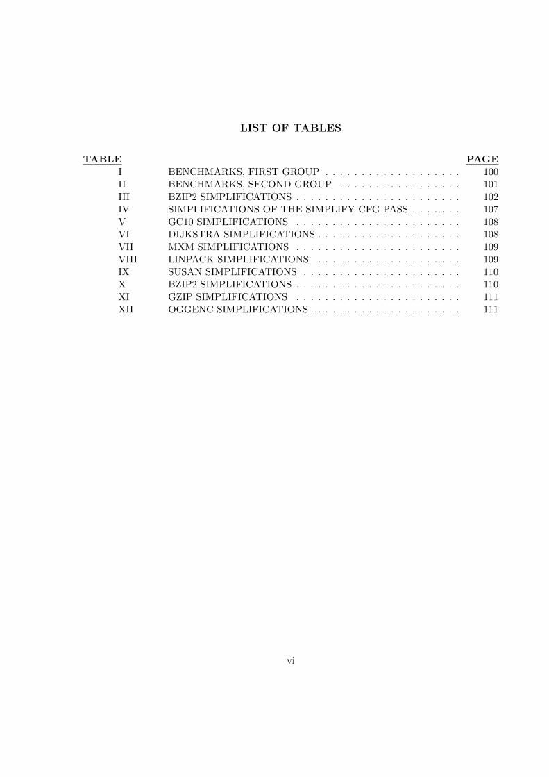
LIST OF TABLES

TABLE PAGEI BENCHMARKS, FIRST GROUP . . . . . . . . . . . . . . . . . . . 100II BENCHMARKS, SECOND GROUP . . . . . . . . . . . . . . . . . 101III BZIP2 SIMPLIFICATIONS . . . . . . . . . . . . . . . . . . . . . . . 102IV SIMPLIFICATIONS OF THE SIMPLIFY CFG PASS . . . . . . . 107V GC10 SIMPLIFICATIONS . . . . . . . . . . . . . . . . . . . . . . . 108VI DIJKSTRA SIMPLIFICATIONS . . . . . . . . . . . . . . . . . . . . 108VII MXM SIMPLIFICATIONS . . . . . . . . . . . . . . . . . . . . . . . 109VIII LINPACK SIMPLIFICATIONS . . . . . . . . . . . . . . . . . . . . 109IX SUSAN SIMPLIFICATIONS . . . . . . . . . . . . . . . . . . . . . . 110X BZIP2 SIMPLIFICATIONS . . . . . . . . . . . . . . . . . . . . . . . 110XI GZIP SIMPLIFICATIONS . . . . . . . . . . . . . . . . . . . . . . . 111XII OGGENC SIMPLIFICATIONS . . . . . . . . . . . . . . . . . . . . . 111

vi

LIST OF FIGURES

FIGURE PAGE1 Witnessing CFG optimizations . . . . . . . . . . . . . . . . . . . . . . 42 Schema for the witness generation . . . . . . . . . . . . . . . . . . . . 73 Structure of a compiler . . . . . . . . . . . . . . . . . . . . . . . . . . . 104 LLVM structure . . . . . . . . . . . . . . . . . . . . . . . . . . . . . . . 135 Example of CFG . . . . . . . . . . . . . . . . . . . . . . . . . . . . . . . 186 Output example . . . . . . . . . . . . . . . . . . . . . . . . . . . . . . . 287 Example of FoldBranchToCommonDest . . . . . . . . . . . . . . . . . 318 Example of RemoveUnreachableBlocks . . . . . . . . . . . . . . . . . . 329 Example of TurnSwitchRangeIntoICmp . . . . . . . . . . . . . . . . . 3310 Source and target parts of a witness relation . . . . . . . . . . . . . . 3711 The witness general model . . . . . . . . . . . . . . . . . . . . . . . . . 3812 Removing a basic block . . . . . . . . . . . . . . . . . . . . . . . . . . . 4313 Merging basic blocks . . . . . . . . . . . . . . . . . . . . . . . . . . . . . 4514 Jump threading . . . . . . . . . . . . . . . . . . . . . . . . . . . . . . . . 4815 Instruction replacement . . . . . . . . . . . . . . . . . . . . . . . . . . . 4916 SimplifyEqualityComparisonWithOnlyPredecessor: conditional branch 5417 FoldValueComparisonIntoPredecessors: case 1 . . . . . . . . . . . . . 5618 FoldValueComparisonIntoPredecessors: case 2.1 . . . . . . . . . . . . 5819 SimplifyBranchOnICmpChain: disjunction of eq comparisons . . . . 6020 FoldBranchToCommonDest: conjunction . . . . . . . . . . . . . . . . 6221 HoistThenElseCodeToIf: hoist of the terminator . . . . . . . . . . . . 6422 SpeculativelyExecuteBB: an example . . . . . . . . . . . . . . . . . . . 6623 FoldCondBranchOnPHI: an example . . . . . . . . . . . . . . . . . . . 6824 SimplifyCondBranchToCondBranch: an example . . . . . . . . . . . . 7025 SimplifyEqualityComparisonWithOnlyPredecessor: case 1 . . . . . . 7326 SimplifySwitchOnSelect: example for conditional branch . . . . . . . 7527 TurnSwitchRangeIntoICmp: an example . . . . . . . . . . . . . . . . . 7728 EliminateDeadSwitchCases: an example . . . . . . . . . . . . . . . . . 7929 SwitchToSelect: an example . . . . . . . . . . . . . . . . . . . . . . . . 8130 ForwardSwitchConditionToPHI: an example . . . . . . . . . . . . . . 8331 SinkThenElseCodeToEnd: an example . . . . . . . . . . . . . . . . . . 8532 TryToSimplifyUncondBranchWithICmpInIt: case 3 . . . . . . . . . . 8733 FoldBranchToCommonDest: unconditional branches, case 1 . . . . . 9034 SimplifyCondBranchToTwoReturns: an example . . . . . . . . . . . . 9135 FoldTwoEntryPHINode: an example . . . . . . . . . . . . . . . . . . . 9436 MergeEmptyReturnBlocks: an example . . . . . . . . . . . . . . . . . 95

vii

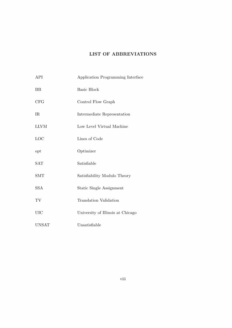
LIST OF ABBREVIATIONS

API Application Programming Interface

BB Basic Block

CFG Control Flow Graph

IR Intermediate Representation

LLVM Low Level Virtual Machine

LOC Lines of Code

opt Optimizer

SAT Satisfiable

SMT Satisfiability Modulo Theory

SSA Static Single Assignment

TV Translation Validation

UIC University of Illinois at Chicago

UNSAT Unsatisfiable

viii

ABSTRACT

Proving the correctness of a program transformation, and specifically, of a compiler op-

timization, is a long-standing research problem. Trusting the compiler requires to guarantee

that the properties verified on the source program hold for the compiled target-code as well.

Thus, the primary objective of formal correctness verification is to preserve the semantics of

the source code, maintaining untouched its logical behavior.

Traditional methods for formal correctness verification are not convenient to validate large

and complex programs like compilers [1], and intensive testing, despite its proven efficacy,

cannot guarantee the absence of bugs [2].

This thesis is part of a larger on-going research project aimed to demonstrate the feasibility

to overcome the difficulties of traditional formal methods. K. Namjoshi and L. Zuck [3] propose

a new methodology for creating an automated proof to guarantee the correctness of every

execution of an optimization. A witness is a run-time generated relation between the source

code and the target code, before and after the transformation. The relation is able to represent

all the properties that must be valid throughout the optimization, offering a mathematical

formula to prove, through a SMT-Solver (typically Microsoft Z3 ), if the invariants hold and

the semantics is preserved.

This work is a further step towards the implementation of a witnessing compiler [4]: the

SimplifyCFG pass of the LLVM compiler framework is augmented with a witness generator

ix

ABSTRACT (continued)

procedure which constructs, run-time, the relations to prove the correctness of every single

simplification in the control flow graph, performed by the compiler.

We show that it is feasible to augment the SimplifyCFG pass with a witness generation

procedure. We describe the structure of the code and the mathematical relations designed to

demonstrate the correctness of a transformation on the Control Flow Graph. Benchmarks and

tests will prove the correct behavior of our implementation and the effectiveness of the witness-

ing procedure. We provide details about the witnesses and the results of the benchmarks.

First, the problem is described, together with the limitations of the traditional methods; then

a solution is designed and explained. Details about the actual implementation for the Simpli-

fyCFG code are provided in further sections.

x

AMPIO ESTRATTO

Provare la correttezza del software e argomento di ricerca a lungo fonte di dibattito. I metodi

formali tradizionali sono complessi, richiedono ampie conoscenze tecniche e non sono adatti a

dimostrare la correttezza di grandi programmi. Il migliore esempio per mostrare l’inadeguatezza

dei metodi classici e rappresentato dai compilatori: estesi software di traduzione del codice i

quali adottano tecniche di analisi e ottimizzazione matematiche complesse.

La compilazione costituisce una fase fondamentale nello sviluppo del software, poiche tra-

duce il codice sorgente dal linguaggio di alto livello ad un linguaggio specifico per l’architettura

del calcolatore. Questa traduzione e una trasformazione del programma in input, il source, nel

programma in output, il target.

La correttezza di un compilatore e particolarmente importante da verificare, esso puo in-

trodurre errori silenti che non sono individuabili ne correggibili dal programmatore, il quale si

concentrera sul proprio codice, avendo piena fiducia nella trasformazione effettuata. Soddisfare

la fiducia riposta nella trasformazione significa garantire che le proprieta del codice sorgente

siano valide anche nel codice target.

LLVM e un framework di compilazione che ottimizza il codice sorgente per avere un pro-

gramma finale il piu efficiente e veloce possibile. LLVM e costituito da una parte di front-end,

rappresentata dal compilatore clang, e una parte di back-end che costituisce l’ottimizzatore vero

e proprio. Il sistema e modulare, diviso in una sequenza di passi di ottimizzazione nella quale

l’output di un passo e l’input del passo successivo. Tutti i passi operano sulla rappresentazione

xi

AMPIO ESTRATTO (continued)

intermedia propria del framework, risultato della compilazione effettuata da clang a partire dal

codice di alto livello in ingresso. La rappresentazione intermedia e in forma SSA, static single

assignment, la quale abilita un numero elevato di ottimizzazioni. SSA significa che ogni vari-

abile deve sempre essere definita prima di essere utilizzata, ma soprattutto puo essere definita

una sola volta. Ogni modifica al valore della variabile costituisce la creazione di una nuova

versione della stessa. L’immediato risultato e l’unicita delle variabili: si puo essere certi che

due variabili con lo stesso nome sono in realta la stessa variabile, nella stessa versione. Tutti

i passi dell’LLVM agiscono sulla rappresentazione intermedia, e mantengono la proprieta SSA

del codice ad ogni modifica effettuata.

Garantire la correttezza di una compilazione significa quindi garantire che la semantica del

programma in ingresso resti invariata attraverso tutte le ottimizzazioni effettuate.

Esistono generalmente due metodologie per verificare la correttezza di una trasformazione:

verificare il codice del compilatore o verificarne l’output. La prima metodologia richiede ampie

conoscenze delle tecniche formali di verifica del software e cerca di sviluppare metodi adatti ad

ogni input dell’insieme degli input possibili. La seconda, chiamata anche Translation Validation,

si pone l’obiettivo di confermare la validita di una traduzione confrontando il programma in

ingresso con il programma in uscita, senza porre l’attenzione sul codice stesso del compilatore.

Translation Validation tuttavia non e precisa, in quanto adotta delle euristiche per dichiarare

l’eguaglianza semantica del programma prima e dopo la trasformazione.

Kedar Namjoshi e Lenore Zuck propongono un metodo alternativo per generare prove au-

xii

AMPIO ESTRATTO (continued)

tomatiche della correttezza di una trasformazione. Questo nuovo approccio si colloca nel mezzo

delle comuni metodologie: non si cerca di verificare la correttezza del codice ne si applicano eu-

ristiche, tuttavia, la conoscenza dell’implementazione e fondamentale e la verifica della trasfor-

mazione avviene run-time, non su tutti gli input possibili, ma sulla specifica corrente esecuzione

del passo di ottimizzazione.

Il nuovo metodo consiste nella generazione di una witness per ogni esecuzione della trasfor-

mazione. La witness e una relazione matematica che lega il codice source con il codice target, e

una formula logica del primo ordine in grado di rappresentare tutte e sole le modifiche apportate

al codice in input. La witness sara composta da due parti, una per il codice in ingresso e l’altra

per il codice in uscita. Se complessivamente la formula logica e valida, allora la trasformazione

puo essere dichiarata corretta.

La verifica della validita della formula witness viene effettuata da un SMT-Solver, nel nostro

caso Microsoft Z3, il quale dichiara le formule in input come soddisfacibili SAT o insoddisfaci-

bili UNSAT.

Questa tesi si colloca all’interno di un progetto piu ampio rivolto alla creazione di un wit-

nessing compiler, nel quale tutti i passi di ottimizzazione sono stati forniti di una procedura

automatica di generazione delle witness.

Il passo analizzato in questa tesi e il SimplifyCFG pass, il quale si occupa della semplifi-

cazione e ottimizzazione del Control Flow Graph della rappresentazione intermedia generata da

clang a partire dal codice sorgente di alto livello in ingresso. Il CFG e un grafo che rappresenta

xiii

AMPIO ESTRATTO (continued)

il flusso delle possibili esecuzioni del programma. Un percorso nel grafo costituisce una singola

possibile esecuzione. Il CFG e composto da basic block terminanti con una istruzione capace

di trasferire il controllo ad un blocco successivo. Un blocco possiede il controllo quando le

istruzioni contenute al suo interno vengono eseguite.

Il SimplifyCFG effettua le ottimizzazioni analizzando la struttura del grafo e le istruzioni con-

tenute nei blocchi. Semplificazioni comuni sono la rimozione di blocchi irraggiungibili o la

sostituzione di istruzioni complesse, come gli switch, con istruzioni piu semplici, come i branch.

Il codice del passo e stato fornito di una procedura automatica che raccoglie run-time le

informazioni necessarie a generare la witness. La relazione cattura tutte e sole le modifiche

effettuate, senza prendere in considerazione le parti del codice che non vengono alterate. Cio

garantisce estrema semplicita della formula logica della witness, in quanto le ottimizzazioni

effettuate sul grafo non sono globali, ma locali a piccole e precise configurazioni del CFG.

Oltre alla procedura, e stato inserito un sistema di variabili statistiche che restituiscono la

tipologia e il numero delle semplificazioni effettuate. Queste statistiche risultano fondamentali

per monitorare il comportamento del passo e della procedura implementata.

Il codice della procedura automatica, e del compilatore stesso, e stato testato durante tutto

il processo di sviluppo. Isolare la precisa semplificazione e fondamentale per essere sicuri di

generare la witness solo per la trasformazione in analisi. A tal proposito sono state scritte delle

semplici funzioni di codice C in grado di far eseguire solo ed esclusivamente la parte del passo

xiv

AMPIO ESTRATTO (continued)

da verificare. Bisogna pero notare che molte volte i casi di semplificazione sono sovrapposti,

quindi e stato necessario disattivare le trasformazioni non volute, modificando di volta in volta

il codice. Specifici benchmarks sono stati infine utilizzati per testare l’efficacia della procedura

automatica e la correttezza del compilatore.

Durante le fasi di sviluppo, testing e benchmarking, non sono mai stati riscontrati errori nel

codice del SimplifyCFG. Non significa tuttavia che il passo sia privo di errori, ma che non sono

state introdotte incorrettezze negli specifici casi testati. Nelle appendici di questa tesi e possi-

bile trovare tutti i risultati delle compilazioni dei benchmarks.

In questa tesi e quindi stato dimostrato che implementare una procedura automatica di gener-

azione di witness e possibile per un generico passo di ottimizzazione. Estendere la metodologia

a tutti i passi di LLVM costituisce un prossimo lavoro futuro per raggiungere l’obiettivo prefisso

della creazione di un witnessing compiler.

xv

CHAPTER 1

LLVM AND WITNESSES

1.1 Introduction

Proving the correctness of a program transformation, and specifically, of a compiler op-

timization, is a long-standing research problem. Trusting the compiler requires to guarantee

that the properties verified on the source program hold for the compiled target-code as well.

Thus, the primary objective of formal correctness verification is to preserve the semantics of

the source code, maintaining untouched its logical behavior.

Commonly, mostly among industries, correctness is the right implementation into software

of requirements and specifications, hence, their only effort is verifying that the high level behav-

iors of programs is compliant with those high level functional and non-functional requirements.

Optimizing compilers not only translate high level programming languages into low level ma-

chine code, but perform optimizations and transformations on the code itself, introducing new

possible sources of errors and bugs. Ensuring the formal correctness of the implemented code

is no more sufficient to validate the software. There is now a growing awareness of the need to

verify the correct translation of the high level source code into the low level target code [5].

There are mainly two different common strategies to validate the correctness of the trans-

formations: validating the code of the compiler or validating the translations performed.

1

2

The first strategy, more traditional, aims to verify the code of the compiler in order to

validate every single transformation on the whole set of legal input programs. This strategy,

expensive and time-consuming, requires expert engineers with deep knowledge of mathematical

theorem-proving techniques, since modern compilers adopt very sophisticated analysis and op-

timization algorithms. Traditional methods for formal correctness verification are not feasible

to validate large and complex programs like compilers [1], and intensive testing, despite its

proven efficacy, cannot guarantee the absence of bugs [2].

The formal correctness verification of optimizing compilers is challenging, not only due

to their size, but also because of their fast evolution which makes any possible proof quickly

outdated.

The second strategy consists in validating the output of the compiler, declaring the transla-

tion as correct. This kind of techniques, named Translation Validation [5], is a simpler approach

than the traditional techniques: the compiler code is not directly verified, but instrumented

with a validating tool that, after every run of the compiler, confirms the correctness of the

target code produced. This techniques are therefore independent of the specific compiler code

and do not require the full mathematical knowledge of the algorithm actually adopted.

K. Namjoshi and L. Zuck [3] propose a new methodology for creating an automated proof

to guarantee the correctness of every execution of the optimization. This novel approach is not

aimed to verify the compiler code itself nor employs heuristics to generate a relation for every

instance of an unknown translation, as for translation validation techniques.

3

With this new method, the compiler code is augmented with a witness generation procedure

to generate a witness relation, the core of this methodology. A witness is a run-time generated

relation between the source code and the target code, able to represent all the properties that

must be valid throughout the optimization, offering a mathematical formula to prove, through

a SMT-Solver (typically Microsoft Z3 ), if the invariants hold and the semantics is preserved.

Differently from the translation validation technique, witnessing a program transformation does

not mean to validate the translation without knowing the transformation performed, and, dif-

ferently from traditional formal methods, there is not the need to directly verify the code of

the compiler. Rather, the witness procedure gathers hints on the compiler behavior, exploiting

all the static analysis accomplished by the optimization, and then collecting the information

necessary to bind the source and the target codes in a witness relation, specifically built for the

current run of the compiler. The compiler code is therefore not formally verified for all possible

input programs, but the current translation, augmented with the witness relation, is confirmed

to be correct.

In this work, the witnessing procedure is applied to the simplifications performed by the

Low Level Virtual Machine compiler framework on the Control Flow Graph of the Intermediate

Representation of the source program. Witnessing the SimplifyCFG pass of the LLVM is a

further step in the implementation of a witnessing compiler [4].

Figure 1 offers a complete overview of this thesis work. The witness generator is added

to the SimplifyCFG pass of the LLVM optimizer in order to gather information about the

optimizations which transform the source program into the target program. The pass, as

4

Figure 1: Witnessing CFG optimizations

5

indicated by the LLVM profiling statistic variables, is one of the most frequent executed. The

generator procedure we added, creates a witness relation between the invariant properties of

the source and the target codes. The witness is then submitted to the SAT-solver Z3 and its

validity is checked.

In the next sections, the witnessing methodology is described in further details, and a com-

plete overview of the LLVM and the SimplifyCFG pass is given.

1.2 The Witnessing Methodology

Traditional formal methods are impractical for large software systems. We have seen that

it is very hard to verify a transformation on the whole set of legal input programs.

To overcome this limitation, K. Namjoshi and L. Zuck [3] propose a witnessing methodology :

the transformation pass is augmented with a witness generating procedure, able to define a

relation between the source and the target programs. A witness is a run-time generated relation

which represents all the properties that must be valid before and after an optimization in order

to assert the correctness of the transformation. This novel approach is an easier method to carry

an invariant through the transformation, from the source program to the target program.

Instead of proving the correctness of the transformation on all the possible inputs, the

witness methodology aims at guaranteeing the correctness of the single execution instance.

While it is expensive and difficult to find all the solutions of a problem, it is much easier to

understand if a candidate solution is indeed a solution. In the first case we may need to find

6

a general mathematical formula to find all the solutions, in the second case we only need to

check the candidate against the definition of a solution, which is already known.

Let the source program to optimize be Ps and the optimized program be Pt, a transforma-

tion T is defined as a relation between the source program and the target program, such that

Pt = T (Ps). Given a transformation T and the set of invariants I, a witness W is a relation

W : (Ps × T × I)→ (Pt × I) where I is the set of all properties which hold for the source pro-

gram and, in order to guarantee the correctness of the transformation, must hold for the target

program as well. A witness can thus be defined over the transformation (Ps, I) = T (Pt, I). If all

the properties of the source code are valid after the transformation also in the target code, the

optimization has been performed correctly, without altering the semantics of the original input.

1.2.1 Witness Generation

The generation of a witness is performed through a witness generator which is added to

the code of the transformation. Differently from the Translation Validation techniques, we are

not employing heuristics to generate a relation between instances of an unknown translation,

but we are directly operating on the code of the optimization, instrumenting it with the code

of the generator. This approach allows us to exploit all the static analysis performed by the

optimizing pass, making our witness more precise, and generating the relation only when it is

actually needed and only over the code modified by the transformation, not over all program

even if untouched. The generator, since it is directly plugged into the optimizing code, can

7

observe the behavior of the transformation, and collect just the amount of information needed

to build the smallest relation possible.

The great advantage of the witnesses is also that, even though we are operating directly

on the code, the methodology is not strictly related to one particular optimization, but can be

applied in the same way to all kinds of transformation passes, designing the right mathematical

relation to catch all and only invariants needed to assert the correctness of the transformation.

Figure 2: Schema for the witness generation

In the Figure 2 we observe the whole schema for the witness generation. The source program

Ps is the input of the transformation procedure which has the target program Pt as output.

The source program holds the set of properties I which is an invariant for the optimization

8

procedure, and thus, it must hold also for the target code. During the optimization phase, the

witness generator produces the witness, a relation between the invariants of the two programs.

1.2.2 Checking Witnesses

The target program is declared to be a correct transformation of the source program if the

source semantic is preserved during the optimization. A witness defines a relation between

the target and the source invariants. Checking the correctness of the transformation means

checking the witness to be a valid witness for the transformation and thus that the invariants

hold.

As explained in further details into section 1.5, after generating the witness, we used the

Microsoft SMT-Solver Z3 [6] to check the validity of the witness for a specific instance. Since

the witness relation is generated in the form of a conjunctive logical formula, we exploit the

power of the SMT-solver to check its validity. The solver will return SAT if the transformation

has been performed correctly, UNSAT otherwise.

The witness methodology, applied to real cases, brings the great benefit to manifest the

errors in case they happen. Normally, it is not possible to be aware of the presence of bugs, but

with this improvement, we can reveal errors in the compiler optimization pass that otherwise

would have been propagated silently to the target program, changing the original semantics of

the source code.

9

1.3 Low Level Virtual Machine (LLVM)

The Low Level Virtual Machine, known as LLVM, is an optimizing compiler framework. It

provides a modern SSA compilation strategy based on modular passes, each of them perform-

ing a different optimization on the Intermediate Representation code. The front-end of the

compiler is implemented in the CLANG compiler, while the optimizing code constitutes the

back-end of the framework. In this chapter we will explain which is the architecture of a compiler

and how LLVM is structured. We will go through the SSA definition and we will provide the

background necessary to understand the simplifications performed on the Control Flow Graph.

1.3.1 Structure of a Compiler

The structure of a optimizing compiler framework is typically divided into two sub-systems:

the front-end and the back-end. The front-end of the compiler framework is what we simply

call compiler : it takes as input the source code written in any programming language, parses it,

defines its structure and then translates it into another language, called Intermediate Represen-

tation. The back-end of the framework is more appropriately called optimizer. The optimizer

performs simplifications and optimizations on the IR and at the end of the process, translates

the IR into the executable code, proper for the particular underneath hardware architecture.

The strength of a structure divided into two subsystems is the independence of the back-end

of the particular language used in the source code; the optimizer operates always on the IR

code generated by the front-end, whose task is to recognize the structures and constructs of the

particular programming language used. In the same way, the front-end of the framework just

10

needs to deal with the programming language, independently of the particular architecture of

the systems.

To provide a measure of this strength, if we assume that the front-end can translate into

IR N different high level programming languages and the back-end can generate executable

code for M different architecture, the whole framework is able to compile and translate into

executable code N ×M different combination of languages and architectures.

Figure 3: Structure of a compiler

11

In Figure 3 we have a schema of the structure of an optimizing compiler framework: the

source language is the input of the front-end subsystem, which translates it into intermediate

representation. The IR is then the input of the back-end subsystem, which generates the ma-

chine code.

1.3.2 LLVM Structure

The Low Level Virtual Machine [7], known as LLVM, is an optimizing compiler framework.

It provides a modern SSA compilation strategy based on modular passes, each of them per-

forming a different optimization on the Intermediate Representation code. The front-end of the

compiler is implemented in the CLANG compiler, while the optimizing code constitutes the

back-end of the framework.

CLANG [8], the front-end of the llvm, is a compiler for the C-language family: C, C++,

Objective C, Objective C++. The main design concept of CLANG is its library-based archi-

tecture. In this design, the front-end is divided into separate libraries which are composed to

implement different functionalities. The library-based approach encourages good interfaces and

makes it easier for new developers to get involved. Each library is a tool for a specific purpose;

for instance, liblex is the lexer, libparse is the parser, libcodegen is the library to generate the IR

code, and libanalysis is the library for the static analysis. CLANG is then the driver program,

the client to handle the flow through the use of the libraries.

The back-end of the LLVM performs optimization on the IR code generated by CLANG

and translates the final version of the IR into machine code. The back-end can be ideally

12

divided into to parts, the optimizer, which performs all the optimization on the IR, and the

code generator, which generates the machine code.

The optimizer is designed with high modularity: it is divided into many different passes,

each of them performing a single type of optimization. All passes are independent of each other

and all operate on the IR code, thus, it is easy to write a new optimization pass and plug it

into the LLVM back-end. There is no need to interface the new pass with all the other, the

only necessity is to reason and operate on the intermediate representation.

All the passes of the optimizer are structured in a sequence, a pipeline in which the output of

one pass is the input of the following pass. Each pass analyzes and transforms the source input

program into the target output program; the sequent pass then takes this target program that

becomes now its source program, and so on until no optimizations can be performed anymore.

The common interface for all the passes is the LLVM intermediate representation itself,

any input programming language is compiled by CLANG into IR code, which is the common

language used by the all components of the LLVM framework. Implementing a new pass is then

simpler, we do not need to know the code of the front-end or of the other passes, we just need

to handle the IR code. The LLVM framework provides many APIs to go through the code in

IR form, without the need to implement new and difficult lexers and parsers.

The main feature of the LLVM intermediate representation is Static Single Assignment,

SSA. SSA requires that each variable is assigned exactly once, and no variable can be used

before its definition. This property enables many different optimizations, since we can always

13

be aware that if two variables have the same name, then they are actually the same variable.

Further details about SSA are provided in section 1.3.3.

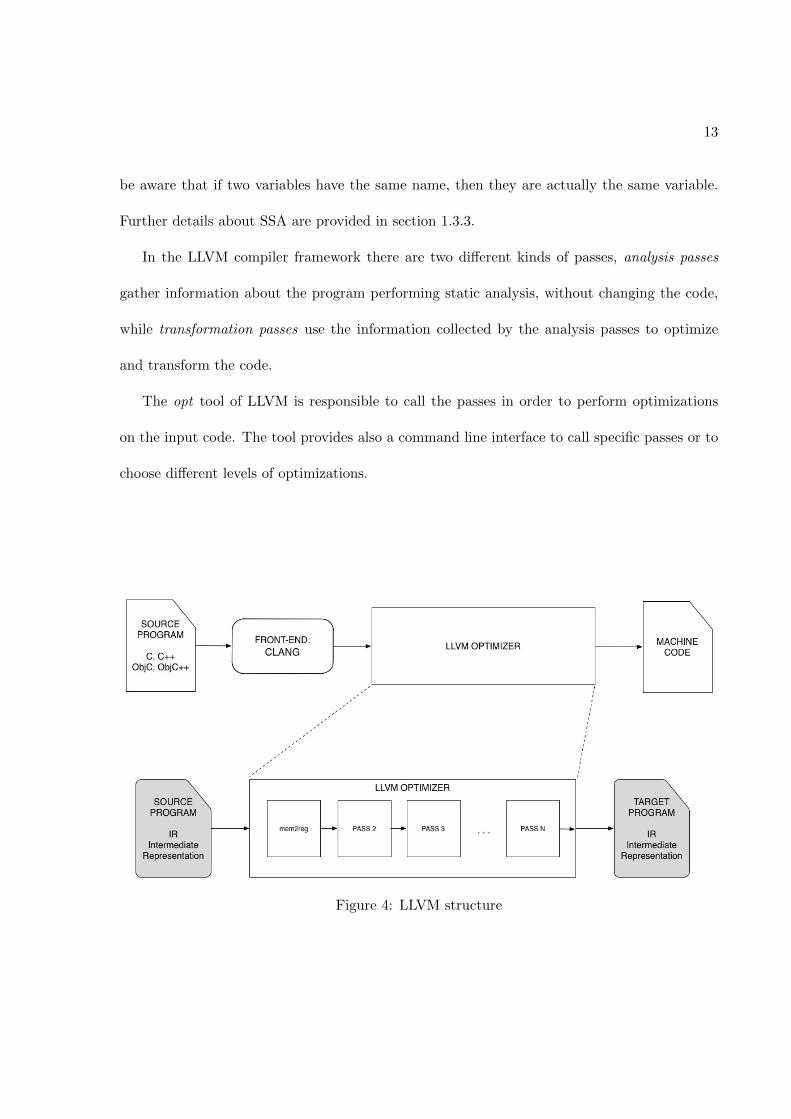
In the LLVM compiler framework there are two different kinds of passes, analysis passes

gather information about the program performing static analysis, without changing the code,

while transformation passes use the information collected by the analysis passes to optimize

and transform the code.

The opt tool of LLVM is responsible to call the passes in order to perform optimizations

on the input code. The tool provides also a command line interface to call specific passes or to

choose different levels of optimizations.

Figure 4: LLVM structure

14

In Figure 4 the architecture of the LLVM framework is presented. First, the program in a high

level programming language (currently, belonging to the C-family) is submitted to CLANG, the

front-end. It translates the code into the LLVM intermediate representation which is the new

input for the back-end. The optimizer, composed by a pipeline of analysis or transformation

passes, transforms and optimizes the code. Once there are no more possible optimizations,

the program, depending on the underneath architecture, is finally translated into executable

machine code.

1.3.3 Static Single Assignment

The IR code of the LLVM framework is in static single assignment form [9] . SSA requires

that each variable is assigned only once, and no variable can be used before its definition.

This property enables many different optimizations, since we can always be aware that if two

variables have the same name, then they are actually the same variable, sharing the same unique

definition.

Static analysis is easy if the code is in SSA property, it is simple to understand which is

the definition of a variable we are using, since it is possible to define the variable only once.

It is straightforward to generate the def-use chain for a variable: the definition is one and all

the following variables with the same name are indeed uses of that variable. We can easily

understand, for instance, where a variable is used and if a variable is used outside a specific

block. This property allows us to perform many optimizations, because we know with precision

if the variable we are modifying has side-effects on another part of the code, in another block.

15

Every time a variable is updated, a new version of the variable is created, typically increasing

a counter in the name of the variable. If two variables are of the same version, it means that

they have the same definition, thus, they are the same variable.

SSA property brings many benefits to static analysis: use-def chains generation, constant

propagation, strength reduction or value range propagation are examples of procedures strongly

enhanced in time and space complexity.

In the LLVM compiler framework, the input code is transformed into SSA form by the

clang front-end and the mem2reg pass of the optimizer. The memory to register pass promotes

memory accesses (load and store operations) to accesses to registers. This pass is the first

optimization called on the compiled code, in order to complete the transformation into SSA

form and enable all the other further optimizations. Throughout the whole execution of the

optimizer, every single function is designed to maintain the SSA form of the IR. At the end of

the optimizations, the SSA form of the IR is converted into machine code.

1 . . . . . .

2 x = a + b; x1 = a + b;

3 x = x + c; x2 = x1 + c;

4 y = x + 2; y1 = x2 + 2;

5 z = x * y; z1 = x2 * y1;

6 . . . . . .

Listing 1.1: Transformation into SSA

1 . . .

2 %add = add i32 %a , %b

3 %add1 = add i32 %add , %c

4 %add2 = add i32 %add1 , 2

5 %mul = mul i32 %add1 , %add2

6 . . .

Listing 1.2: Example of IR code

In listings 1.1 we have a simple example of transformation into SSA form. We can see that

a new variable is created at every new assignment, with an increasing counter that ensures

uniqueness. In Listing 1.2 we can see the actual IR code. In LLVM variables usually take the

16

name of the operation whose result is the value assigned.

1.4 Simplification of the Control Flow Graph

The Control Flow Graph represents all the possible execution paths traversed by a program

during the execution. When a node is visited, its instructions are executed and then the control

passes to another block. Each path represents a particular flow of control. The SimplifyCFG

is the pass of the LLVM compiler framework which simplifies and optimizes the CFG of the IR

code.

In the next sections we will see what a control flow graph is and how it is structured, with

reference to the LLVM framework. In chapter 2 we will go through the different classes of

optimizations and their witnesses. In chapter 3 we will analyze all the simplifications of the

SimplifyCFG.

1.4.1 Control Flow Graph

The Control Flow Graph represents all the possible execution paths traversed by a program

during the execution. Nodes of the graph are basic blocks containing all the instructions exe-

cuted when the node is visited. At the end of each node, the control is passed to the next block,

possibly depending on a condition resulting in a jump to another node which is executed. Each

path represents a chain of basic blocks that are visited in a precise order for a particular run

of the program. The CFG analyzed by the LLVM optimizer is the graph generated from the

IR code, the intermediate representation format of the framework. All programs are translated

17

by CLANG from the higher level programming language into IR code. The optimizer offers a

simple command to generate a visualization of the CFG, as in Listing 1.3. The output of the

program in listing 1.4 is represented in Figure 5

1 opt -view -cfg helloCFG.s

Listing 1.3: CFG visualization command

1 int main (int argc , char* argv []){

2 int var = 0;

3 int res = argc;

4 if (res > 10){

5 var = 10;

6 }else{

7 var = 20;

8 }

9 res = var;

10 return res;

11 }

Listing 1.4: helloCFG.c

Figure 5 is a good starting point to analyze the features of the CFG in the specific case of the

LLVM IR. The CFG is composed of basic blocks linked together by directed arrows representing

the flow of control. Each block and each instruction may have a name and the first block of the

CFG, without parents, is the entry block. All the blocks of the graph end with a terminator

instruction whose task is to transfer the control to the next block, sometimes depending on a

condition. At the beginning of the block there may be one or more PHI nodes. PHI nodes are

the LLVM representation of the φ -function required for the SSA form described in section

18

Figure 5: Example of CFG

1.3.3. After this general introduction, we can analyze the most important instructions of the

LLVM IR.

• Comparison Instruction:

This class of instructions returns a boolean value based on the comparison of two

integers, for icmp, or two floats, for fcmp. The instruction takes three operands, the first

is the condition code indicating the type of operation: (equal eq, not equal ne, greater

than gt, lower than lt, . . . ), the second and the third ones are the two values, of identical

types, to be compared. In Listing 1.5 an example of equality integer comparison. The

19

result of the comparison is stored in the variable %cmp. The type of the operands is

indicated by i32 (32 bit integers).

1 %cmp = icmp eq i32 %var1 , %var2

Listing 1.5: Comparison instruction

• Branch Instruction:

It is a terminator instruction that can appear as last instruction of a basic block.

It transfers the control to the next block. If the next block is chosen depending on

the outcome of a condition, the instruction is a conditional branch, otherwise it is an

unconditional branch. The conditional branch takes the condition for the jump and the

two possible destinations, the first destination is the true destination, while the second

one is the false destination. The unconditional branch just makes the flow to jump to

the only basic block passed to the instruction. In Listing 1.6 we provide an example of

conditional and unconditional branches.

1 br i1 %cond , label %trueDest , label %falseDest

2 br %onlyDestination

Listing 1.6: Branch instructions

• Switch Instruction:

This is a generalization of the branch instruction. It can take more than two blocks as

destinations and transfers the control on the basis of an integer comparison. If the variable

compared is not one of the cases of the switch, the control is transferred to a default basic

20

block. The instruction takes as arguments a variable, different value-destination pairs and

a default destination. In Listing 1.7 an example of switch instruction.

1 switch i32 %var , label %defaultBB [

2 i32 0, label %destOnZero

3 i32 1, label %destOnOne

4 i32 2, label %destOnTwo

5 ]

Listing 1.7: Switch instruction

• Select Instruction:

This instruction is used to choose one of two values depending on a condition, without

the need of a branch. The chosen value is stored in a variable. In Listing 1.8 and example

of select instruction.

1 %resultvariable = select i1 %cond , i32 10, i32 20

Listing 1.8: Select instruction

• PHI node instruction:

PHI nodes are the LLVM IR representation of the SSA φ -function. The phi

instruction takes value-basic block pairs as arguments, one pair for each predecessor block.

When the flow of control can reach a block from more than one predecessor, we need to

know which value of a variable is the correct one that needs to be used in the common

descendant. A PHI node is always placed at the beginning of the block (together with

other possible PHI nodes, one for each variable) and decides which value to take into

21

account, depending on the block the flow is coming from. An example of PHI instruction

is provided in Listing 1.9.

1 %result = phi i32 [%val1 , %BB1],[%val2 , %BB2],[%val3 , %BB3]

Listing 1.9: PHI node instruction

1.4.2 SimplifyCFG Pass

The SimplifyCFGPass of the LLVM optimizer implements functions to perform simplifica-

tions on the Control Flow Graph, operating on the graph structure or directly on the instructions

used inside the blocks. The pass iterates on all the basic blocks of a function and, reasoning

on the predecessors, successors and instructions used inside the current BB, determines if a

particular simplification can be achieved. There are mainly two different methods to analyze

the applicability of an optimization: reasoning on the structure of the CFG or reasoning on

the IR instructions used in the code. In section 2.3 we will analyze these methods in greater

details.

The SimplifyCFG pass recursively simplifies the CFG until no more optimizations can be

executed. It does not simplify the graph as a whole, but recognizes precise patterns in the

structure of the CFG and performs local optimizations. Local optimizations involve a few

number of blocks and instructions, thus transformations are more effective, since the pass does

not need to take into account too many different conditions and side effects. Side effects are

22

indeed local and are easier to handle. Eventually, many different local optimizations lead to a

complete simplifications of the CFG.

The different optimizations are grouped into classes, depending on the terminator instruc-

tion taken into account, or depending on the particular kind of simplification. First, unreachable

blocks (without parents) are removed and immediate optimizations, like removing duplicate PHI

nodes at the beginning of a block are performed. After these basic transformations, the pass

iterates on blocks and reasons on their terminators. Following optimizations, which will be

treated in deep details in chapter 3, involve: Conditional Branches, Unconditional Branches,

Switch Instructions.

1.5 Z3: a SMT-Solver

Z3 is a SMT-Solver developed by Microsoft Research [10]. It is a theorem prover used to

check the satisfiability of logical formulas. Satisfiability Modulo Theory is a decision problem to

check the satisfiability of a formula with reference to some background theories like arithmetics

and function-theory.

A formula is satisfiable if there is an interpretation that makes the formula true. Formulas

can be true or false since they are expressed in first order logic. A formula that can never be true

in any interpretation is unsatisfiable. A SMT-Solver is a tool which can determine if a formula

is SAT or UNSAT. The concept of validity is dual to the concept of satisfiability : a formula that

is true in all structures is said to be valid. The negation of a valid formula is then always false in

any structure and thus unsatisfiable. The SMT adds to the logic concepts common background

23

theories, like addition or subtractions, handling of arrays and uninterpreted functions. Types

are also supported like Integers, Floats or Booleans.

Z3 is a state-of-the-art SMT-Solver used in software verification and analysis applications

[6] [11] . In this thesis we use Z3 to check the witnesses generated by the automatic procedure,

to understand if the transformation performed is correct. The SMT-Solver will return SAT if

the optimization has been executed correctly, UNSAT otherwise. We must notice that there is

the possibility, under particular conditions (typically involving the size of the domains), that

Z3 does not provide any answer. Since the SimplifyCFG pass performs just local optimizations,

the domains of the variables used in the formulas are finite sets, thus the decision problem is

limited and decidable. A finite problem can be modeled using a finite state automaton, which

always leads to an answer.

Logic formulas in Z3 are encoded using SMT-LIB syntax [12]. The syntax adopts the prefix

notation, where operators are placed before their operands. In Z3 it is possible to use typed

variables like Int or Float through the construct:

(declare-const varname Int)

As we can notice, it is necessary, every time, before use, to declare a variable and its type.

This will have a huge impact on the creation of the witnesses, as explained in chapter 3.

It is possible to define custom type with the construct datatypes:

(declare-datatypes () ((TY PE-NAME value1 value2 value3 · · · valuen)))

We must define all the possible values assumed by a variable of the specified custom type.

This is fundamental in order to have a custom bounded domain. The custom bounded set of

24

possible values is particularly important when checking the witness generated: it prevents the

variable to assume an arbitrary value. For this reason we are sure that the output of Z3 will not

be generically SAT in case the antecedent of an implication is false. The bounded domain, if we

enumerate in the witness all the possible implication formulas, for all possible values, prevents

the antecedents to be all false at the same time and thus the final response to be always SAT.

On variables it is possible to perform arithmetic operations like additions or multiplications:

(+ var1 var2) , (∗ var1 var2)

Using boolean conditions, it is possible also to perform logical operations:

(and (= var1 var2) (= var3 var4))

A useful logical operation is the if-then-else statement. It takes three elements. The first is

the condition for the if, the second one is the action of the then block, while the third element

is the else block. If the condition holds, the second element is valid, otherwise the third one is

executed. Here we state that if var1 is equal to var2 then sum var3 to var4, else sum var3 to

var5.

(ite (= var1 var2) (+ var3 var4) (+ var3 var5))

In Z3 all formulas are composed of different sub-formulas, all in a conjunction. We can add

a new conjunctive to the formula using the keyword assert. To check if the whole formula is

satisfiable we need to use the keyword check-sat. It is possible to ask to the solver to provide a

model that satisfies the formula using the keyword get-model.

A very useful feature of Z3 is the presence of a scope-stack of sub-formulas. We can add

or remove sub-formulas using the keyword push and pop. This is particularly useful in case

25

we want to check the current whole formula multiple times, avoiding to add two contradictory

sub-formulas at the same time. We can push a formula in the stack, check it together with other

conjunctives, and then pop it out, add its contradiction and check again. The two contradictory

formulas do not generate a conflict since they belong to two different scopes.

In Listing 1.10 an example of a complete Z3 formula which checks the commutative property

of addition.

1 (declare -const var1 Int)

2 (declare -const var2 Int)

3 (assert (= var1 (+ 1 2)))

4 (assert (= var2 (+ 2 1)))

5 (assert (not (= var1 var2)))

6 (check -sat)

Listing 1.10: Z3 example

CHAPTER 2

WITNESSES AND SimplifyCFG

2.1 Introduction

Witnessing the SimplifyCFG pass of the LLVM is a further step in the implementation of a

witnessing compiler [4]. In this thesis we profiled and analyzed the simplifications of the control

flow graph, instrumented the SimplifyCFG pass and implemented the witnessing procedure to

generate a witness for every single instance of the optimization pass. The procedure provides

witness relations between source and target programs in order to check the correctness of the

simplifications performed.

To check the validity of the witnesses, as we have seen, we exploited the functionalities of

the Microsoft SMT-Solver Z3. Given a conjunction of witnesses, in the form of SMT logical

formulas, the SMT-Solver will return SAT or UNSAT depending on the satisfiability of the

formula, thus, we will understand if the witness generated and analyzed is the relation of a

correct or non correct optimization.

To show the validity of our approach, we run the SimplifyCFG simplifications against bench-

marks, profiling the LLVM code and analyzing the answers of Z3 SMT-Solver. The instrumen-

tation of the code with statistics variables provides information about the frequency of each

optimizations, and about the frequency of the execution of the whole pass.

26

27

In this chapter, we will explain all the phases of the implementation, from the instrumen-

tation of the code with statistics variables, to monitor the simplifications performed, to the

explanation of the classes of simplifications and the design of their typical witnesses.

2.2 Profiling the SimplifyCFG

Profiling the SimplifyCFG means instrumenting the code in order to generate data about

the behavior of the pass, throughout all the optimizations performed. We added statistics

variables that provide information on the number of times the pass is called and the number of

times simplifications are performed.

In the LLVM framework, it is possible to insert specific statistics variables with the macro

STATISTICS and call the optimizer opt, setting the option to retrieve and print those infor-

mation collected during the execution. In Listing 2.1 we can see examples of declarations of

statistics variables while in Listing 2.2 is shown the typical command to perform optimiza-

tions collecting statistics information. The opt is the optimizer which enables the statistics

(-stats) and performs simplifications with the SimplifyCFG pass (-simplifycfg). The optimizer

also generates the IR representation of the target program (-S option) and writes a list of all

simplifications performed with the option -debug-pass=Structure.

1 STATISTIC(Dario_FoldBranchToCommonDest ,

2 "Dario: Dario_FoldBranchToCommonDest");

Listing 2.1: Declaration of a statistic variable

28

1 opt -S -debug -pass=Structure -stats -simplifycfg

2 FoldBranchToCommonDest.s

3 -o FoldBranchToCommonDest_simplifycfg_opt.s

Listing 2.2: Optimization command

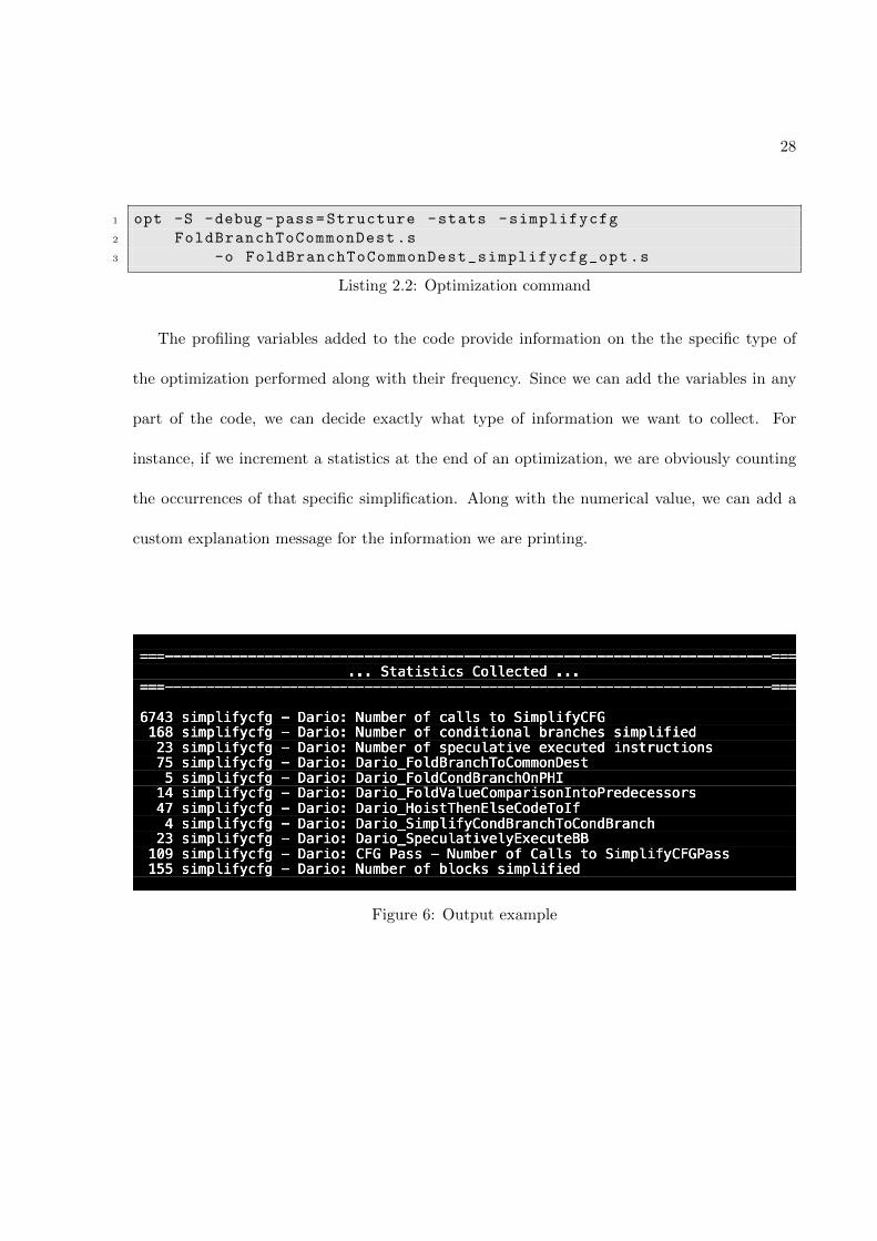
The profiling variables added to the code provide information on the the specific type of

the optimization performed along with their frequency. Since we can add the variables in any

part of the code, we can decide exactly what type of information we want to collect. For

instance, if we increment a statistics at the end of an optimization, we are obviously counting

the occurrences of that specific simplification. Along with the numerical value, we can add a

custom explanation message for the information we are printing.

Figure 6: Output example

29

In Figure 6 there is an example of the output given by the optimizer at the end of the

optimization. We can see the number of times a specific simplification has been performed,

along with the name of the specific pass executed and the custom message for each variable.

2.3 CFG Simplifications

The LLVM compiler framework, as an optimizing compiler, provides a module to optimize

the Control Flow Graph of the IR code. The SimplifyCFG pass of the optimizer implements

functions to perform simplifications on the graph, reasoning on the graph structure or directly

on the instructions used inside blocks. As we have already seen, the CFG of the LLVM is

composed of Basic Blocks connected to each other depending on the flow of control of the code

represented. This means that the graph has a starting block without parents, the entry block,

and each block has a terminator instruction that determines the transfer of control to another

block.

Different classes of terminator instructions can have a different number of following blocks,

and the next one can be determined on the basis of a condition on the run-time values of

variables. The major examples are the Switch Instructions and the Conditional Branches,

which decide the next block evaluating a conditions on some value.

Another important detail to remind, before analyzing the simplifications of the CFG, is

the possible presence of PHI nodes at the beginning of a block. PHI nodes are the LLVM

representations of the φ -function required for the SSA form: when the flow of control can

reach a block from more than one predecessor, we need to know which value of a variable is

30

the current one that needs to be used in the common descendant. A PHI node placed at the

beginning of the block decides which value to take into account, depending on the block the

flow is coming from.

Terminator instructions and PHI nodes are essential to understand the different simplifica-

tions performed and are the core of many different optimizations.

The SimplifyCFG pass of the LLVM iterates on all the basic blocks of a function and, rea-

soning on the predecessors, successors and instructions used inside the current BB, determines

if a particular simplification can be performed. There are mainly two different methods to an-

alyze the applicability of an optimization: reasoning on the structure of the CFG or reasoning

on the IR instructions used in the code.

• Reasoning on the CFG structure:

The Structure of the CFG can suggest many different optimizations; analyzing

predecessors and successors of a block can reveal easy modifications that can simplify

the CFG. For instance, in the FoldBranchToCommonDest, two blocks, a parent node and

its child node, have a common successor and the pass analyzes and understands if the

two blocks can be merged together, and then combines the conditions of their branches

into a single condition, with a logical operator. Indeed, if the two blocks share the same

true destination (and thus the child node is the false destination of the parent node), we

can understand that the second block represents another chance to reach the common

destination and the two conditions can be combined into an OR binary operation. In the

same way, if the two blocks share the false destination, then we can combine them into a

31

logical conjunction. Another easy possible simplification is the RemoveUnreachableBlocks.

If a block has no predecessors, it can be safely removed. In Figure 7 and in Figure 8 we

can see explicative examples of these two simplifications.

Reasoning on the structure of the CFG can lead to the deletion of many branches

and blocks, making the target code faster than the source code, since we have removed

redundant steps in the path to the final block.

Figure 7: Example of FoldBranchToCommonDest

32

Figure 8: Example of RemoveUnreachableBlocks

• Reasoning on the IR instructions:

Execution speed of single instructions, or combination of them, is a key aspect in

reaching an overall better performance. The SimplifyCFG pass can recognize specific

patterns in the usage of the IR code and replace them with a combination of different

simpler and faster instructions. Throughout all the transformations, the SimplifyCFG

pass tries to remove or replace expensive or unneeded instructions, like redundant checking

of conditions or branches. For example, in the TurnSwitchRangeIntoICmp simplification,

when the pass recognizes that all the cases of a switch are part of a range, it replaces

the switch instruction with an integer comparison instruction followed by a conditional

33

branch. In Figure 9 it is shown how the expensive switch is changed into two integer

instructions and a branch.

Figure 9: Example of TurnSwitchRangeIntoICmp

We need to notice that the SimplifyCFG pass handles just those instructions that

can be simplified with a basic knowledge of the structure of the CFG. Indeed, it is not

possible to remove branches to blocks if it is not known that those blocks are empty or

that they do not perform any useful action. SimplifyCFG does not handle the general

replacement of expensive instructions with simpler one; those optimizations are part of

the strength reduction class of optimizations and are optimized by other passes of LLVM.

The SimplifyCFG pass combines these two approaches to the optimization of the graph:

first, the pass analyzes the type of terminator, then, it decides which simplification is applica-

ble, reasoning on the predecessors and successors of the block the terminator belongs to. In

34

chapter 3 we will analyze the different optimizations performed, together with their witnesses.

2.4 Witnesses and Simplifications

Witnessing a simplification is generating a relation between the source code and the op-

timized target code. The witness captures the changes performed by the transformation and

provides evidence of the modifications made by the optimization.

We notice that the SimplifyCFG pass does not optimize the the complete CFG, but rather

performs numerous local optimizations to it, simplifying precise patterns in the graph structure.

All the optimizations of the pass involve just a small number of blocks and instructions, thus,

the witness is generally a simple logical formula in a conjunctive form. Another strength of the

witnessing approach is that the relation does not need to represent parts of the code that do

not change throughout the transformation, but needs to ensure that the parts modified have

been transformed consistently, without changing the semantics of the program.

In section 2.4.1 we will see how a witness is structured and in section 2.4.2 we will study the

general model underneath the witness relation. In section 2.4.3 we explain how we translated

the general model into concrete witnesses for the SimplifyCFG.

2.4.1 Source and Target Programs

An optimizing pass transforms an input program, the source, into an optimized version,

the target. During the optimization, the witness procedure gathers the information necessary

to build the witness relation. To understand the evolution of the program during the trans-

35

formation, the witness relation is composed of two main parts: the source part and the target

part.

The source part of a witness catches the properties of the code at the beginning of the

transformation, before any change. The witness needs to analyze the state of the code before

the transformation in order to understand if the semantics is changed after the modification. We

focus our attention on the variables and their values, as well as the structure of the graph. The

variables are taken into account to study if the target program instructions use the right versions

(version as intended in SSA form) and thus, they use the same definition of the variables. The

structure of the graph is analyzed to follow the flow of control and ensure that the same

conditions lead to the same basic blocks. Indeed, it is possible to change the semantics of a

program not only by changing the values of the variables (or their versions), but also changing

the possible paths through the graph. For this reason, the source part of the witness must

gather the different uses of variables and the possible paths with their conditions. As we said,

there is no need to check variables and paths not involved in the transformation.

The target part of the witness catches the properties of the code right after the optimization,

but before any change due to another simplification. We must be sure to analyze the effects of

only one single transformation at a time.

It is possible that the same transformation method, analyzing the source code structure

and instructions, may decide to perform a variation of the simplification; in this case the target

part of the witness needs to be every time adapted, so, it is possible to have two different

36

witness structures for the same simplification, since the simplification can be implemented with

different approaches.

Source and target parts of the witness are linked in the witness relation through a logic

conjunction. What is valid for the source code must be valid also for the target code in order to

have a correct transformation of the program, where source and target have the same semantics.

Moreover, the flow of control must be changed without removing possible valid paths on the

graph: same conditions must lead to same basic block instructions.

The two parts of the witness are directly linked also by the current values of the variables

used and current names of the basic blocks. For instance, if the control in the source code can

flow from basic block named BB1 to basic block BB2 or basic block BB3 depending on the

outcome of a condition, in the target program, to have a correct transformation, cannot happen

that BB1, through the same condition, goes to a basic block named BB4. The validity of the

whole witness is sometimes determined by the limit number of values a variable can assume; as

we already said, the witness methodology aims at verifying, run-time, the correctness of a single

instance of a transformation, not at developing a relation that can be verified, more generally,

by the set of the all possible input values of the variables.

In Figure 10, we provide a simple visualization of the two parts of the witness.

2.4.2 Witness Model

To prove the correctness of a transformation, we check the validity of the witness relation,

which is a conjunction of the source and target properties. We have seen that a witness relation

37

Figure 10: Source and target parts of a witness relation

collects information about the source and target programs in the form of a logical formula. This

formula contains the properties of the CFG before and after the simplification. Stating that the

target code is a correct transformation of the source code means claiming that the semantics of

the program is not changed throughout the optimization, and thus all the possible paths and

values of the variables are preserved.

As we explained in section 1.4.1, the Control Flow Graph represents all the paths that can

be traversed by the program during its execution. When a block is visited, its instructions are

executed. The flow is determined by conditions and jumps: at the end of each basic block, a

38

terminator instruction, often on the basis of a condition, transfers the control to the next basic

block, which will gain the control of the program.

Figure 11: The witness general model

In Figure 11 we can see an example of generation of a witness. On the left there is the

source code, while on the right there is the target code. We assume that some optimizations

transformed the source into the target program. Each node is marked with its name and con-

tains its condition while the leaves contain the value assignments. We can see how the final

value of the variable var is the same for all paths in both graphs.

39

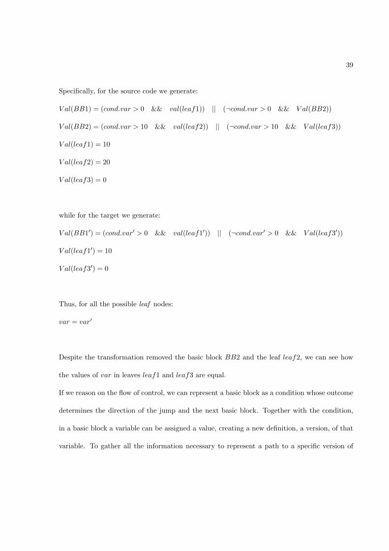
Specifically, for the source code we generate:

V al(BB1) = (cond.var > 0 && val(leaf1)) || (¬cond.var > 0 && V al(BB2))

V al(BB2) = (cond.var > 10 && val(leaf2)) || (¬cond.var > 10 && V al(leaf3))

V al(leaf1) = 10

V al(leaf2) = 20

V al(leaf3) = 0

while for the target we generate:

V al(BB1′) = (cond.var′ > 0 && val(leaf1′)) || (¬cond.var′ > 0 && V al(leaf3′))

V al(leaf1′) = 10

V al(leaf3′) = 0

Thus, for all the possible leaf nodes:

var = var′

Despite the transformation removed the basic block BB2 and the leaf leaf2, we can see how

the values of var in leaves leaf1 and leaf3 are equal.

If we reason on the flow of control, we can represent a basic block as a condition whose outcome

determines the direction of the jump and the next basic block. Together with the condition,

in a basic block a variable can be assigned a value, creating a new definition, a version, of that

variable. To gather all the information necessary to represent a path to a specific version of

40

the variable, we need to retrieve all the assignments and conditions that lead to that specific

version. We can determine a subgraph, which represents a path to a specific use of the variable.

The location of the instruction which is using the version of the variable we are taking into

account can be represented as a leaf (a node without successors), while the starting block of

the path can be considered as the root.

Analyzing the subgraph just determined, we can defined the general model of the witness

for a specific subsection of the CFG. This model is able to represent both the conditions of the

path and the new value assignments.

We define a recursive expression to better understand the general model:

V al(G) = (condition(G1) && val(G1)) || . . . || (condition(Gn) && val(Gn))

V al(leaf) = v′

where G is the root of the subgraph while G1, Gn, is the subgraph whose root is the suc-

cessor node number 1 to number n. In the same way, condition(G1), condition(Gn) is the

condition which determines the block number 1, n to be the next. V al(G) is the final value of

the variable taken into account following the path from the node G, while V al(leaf) is the value

of the variable in case we arrived at the end of the path. v′ is the new value assigned to the vari-

able. To be a witness that is a relation between the source and the target, we need to analyze

the values of the variables and the conditions of the paths, both for the source program and the

target program, for all the variables taken into account. At the end of the analyses, we need to

41

check that the final values (leaf values) of the variables in the source and the target are the same.

Specifically, we obtain:

V ar = Expr(v1, . . . , vn)

and

V ar′ = Expr(v′1, . . . , v′n)

We are showing the two expressions determining the values of the corresponding variable in

the source and the target. If the values are equal,we can conclude the transformation has not

altered the semantics of the code.

Since the witness relation needs to represent only the variables that are involved into the

transformation, and since all the transformations in the SimplifyCFG pass are local, specific for

particular patterns of the CFG, we do not need to take into account many variables and val-

ues, and thus, the witnesses generated take into account, every time, a limited number of values.

In the next section (2.4.3) we will analyze how the general model of the witnesses is declined

into the witnesses for the SimplifyCFG pass.

2.4.3 Witnesses for SimplifyCFG

The optimizations of the SimplifyCFG pass can be grouped into four main classes: Removing

Basic Blocks, Merging Basic Blocks, Jump Threading, Instruction Replacement or Modification.

42

For each of these classes we will provide an explanation and an example of witness relation.

• Removing Basic Blocks:

This class of simplifications operates directly on the CFG structure, deleting one basic

block. A basic block is deleted when it is unreachable, either because it has no prede-

cessors, or the predecessors conditions have not any outcome which leads to the specified

basic block. In these cases, the block can be removed without any side effect, since the

instructions belonging to the block would never have been executed. In the second case,

to remove the block, it is sufficient to remove the edges leading to that block, then, as

in the first case, the block is removed from the list of basic blocks of the function.

The witness for the deletion of the basic block needs to ensure that the remaining paths

and the values of the variables resulting from those paths have not been altered by the

removal. In Figure 12 we show an example. The basic block BB2 is clearly unreachable

because the condition of BB0 can just lead to BB1. BB2 is removed and the witness

checks that the value of the variable var is still 10 and the successor of BB0 is BB1.

Here the witness for the source:

(BB0.Condition ∧ SuccessorBB = BB0.SuccessorTrue ∧ var = 10) ∨

(¬BB0.Condition ∧ Successor.BB = BB0.SuccessorFalse ∧ var = 20)

And the witness for the target:

43

SuccessorBB = BB0.OnlySuccessor ∧ var = 10

If the actual value of BB0.OnlySuccessor in the target code is indeed BB1, the SMT-

Solver will return SAT otherwise it will be not possible to have var = 10 but a basic

block different than BB1.

We note that the only two different values for the constant SuccessorBB are BB1

or BB2, as allowed by the custom datatypes defined in the declaration part of the Z3 file

and described in section 1.5.

Figure 12: Removing a basic block

44

• Merging Basic Blocks:

In particular configurations of the CFG and in the presence of overlapping condi-

tions, two basic blocks can be merged. Typically, a successor block is merged into its

predecessor if the conditions can be put into a logical operation (see the example for

FoldBranchToCommonDest in section 2.3) or of the condition of the predecessor and the

successor overlap. In Figure 13 there is a third pattern that allows the merge of two

BBs. In the example, defBB0 is merged into its predecessor BB0, hoisting its instruction.

This is possible because both the basic blocks end with a switch instruction on the same

variable var. Since the successor is the default destination of the predecessor switch, the

cases of defBB0 can be hoisted into the cases of BB0.

The source part of the witness will be:

(var = BB0.case1.value ∧ SuccBB = BB0.case1.dest) ∨

(var = BB0.case2.value ∧ SuccBB = BB0.case2.dest) ∨

(var = defBB0.case1.value ∧ SuccBB = defBB0.case1.dest) ∨

(var = defBB0.case2.value ∧ SuccBB = defBB0.case2.dest) ∨

(var /∈ (BB0.cases ∪ defBB0.cases) ∧ SuccBB = defBB0.default)

And the witness for the target code:

(var = BB0.case1.value ∧ SuccBB = BB0.case1.dest) ∨

45

(var = BB0.case2.value ∧ SuccBB = BB0.case2.dest) ∨

(var = BB0.case3.value ∧ SuccBB = BB0.case3.dest) ∨

(var = BB0.case4.value ∧ SuccBB = BB0.case4.dest) ∨

(var /∈ BB0.cases ∧ SuccBB = BB0.default)

If the values of the cases and their destinations are correctly merged into the prede-

cessor switch instruction, then the witness is a relation of a correct optimization and no

cases have been lost during the transformation.

Figure 13: Merging basic blocks

46

• Jump Threading :

This is a well-known class of optimizations. The compiler changes the destination

of a jump, turning a conditional branch into an unconditional branch, or redirecting the

branch to the successor of the successor, thus, skipping a block. This can happen when

the successor condition is a subset of the predecessor one or is completely determined by

the predecessor condition outcome. This means that the successor condition is redundant,

since we know already its outcome during the execution of the predecessor. The successor

branch is always taken if the predecessor condition is a super-set of the condition of the

successor, while the branch is never taken if the two conditions are mutually exclusive.

It is possible and safe to skip the evaluation of a condition and address the first jump

directly to the real destination.

In Figure 14 we show an example of jump threading. The condition of the inte-

ger comparison in BB2 is already determined since the origin of the incoming edge is a

switch where the same condition has been already evaluated. We can change the des-

tination block of the switch case of BB0 into the successor of BB2, skipping BB2 and

performing jump threading to BB3. BB2 is not removed by this simplification, but, since

now unreachable, it will be removed by following steps of the whole optimization pro-

cess. We can now reason on the witness relation. We need to retrieve from the source

program, after an analysis of the code, the real destination of the switch case, to com-

pare this real destination to the destination of the modified switch case in the target code.

47

The source program generated the following formula:

(var = BB0.case1.value ∧ SuccBB = BB0.case1.dest) ∨

(var = BB0.case2.value ∧ SuccBB = BB2.truedestination) ∨

(var /∈ BB0.cases ∧ SuccBB = BB0.default)

The formula for the target code is:

(var = BB0.case1.value ∧ SuccBB = BB0.case1.dest) ∨

(var = BB0.case2.value ∧ SuccBB = BB2.case2.dest) ∨

(var /∈ BB0.cases ∧ SuccBB = BB0.default)

If the real destination retrieved from the source code is actually the same destination of

BB0.case2.dest, then we can assume the jump threading has been performed correctly.

• Instruction Replacement or Modification:

The SimplifyCFG identifies specific patterns in the code and evaluates whether some

instructions can be modified or replaced. See Figure 15 for an example where we have

a switch instruction with a single successor. Basic blocks BB1 and defBB are empty,

they have just an unconditional branch to BB2. In BB2 a PHI node picks the right

value depending on the incoming block. In this pattern, BB1 and defBB are just used to

initialize the value into the PHI node. The transformation replaces the switch instruction

48

Figure 14: Jump threading

with a select instruction preceded by an integer comparison. The final conditional branch

is transformed into an unconditional branch. With this modification, other optimizations

are enabled and BB1 and defBB are removed. The resulting CFG is simpler and the

target code optimized. We can now analyze the witness relation.

The source program generates:

(var = BB0.case1.val ∧ phi.val = phinode.incomingBB1.val) ∨

(¬(var = BB0.case1.val) ∧ phi.val = phinode.incomingpredBB.val)

The target part of the witness is instead:

49

(var = select.trueval ∧ phi.val = select.var) ∨

(var = select.falseval ∧ phi.val = select.var)

Figure 15: Instruction replacement

50

The transformation is correct if the select handles properly the values of the switch cases

and the substitution of the select.var into the PHI node is accurate.

CHAPTER 3

WITNESSING CFG OPTIMIZATIONS

In this chapter we will analyze the simplifications performed by the SimplifyCFG and their

typical witnesses.

3.1 Introduction

A witness is composed of two main parts: the part for the source code and the part for the

target code. Both components are expressed as a conjunction, which renders their checking

in Z3 simple. From the implementation point of view, because of the constraints imposed

by the Z3, a witness is divided into a declaration part and a formulation part. Z3 requires

that a variable appearing in the formula is earlier declared, together with its type. In case

we need to define a new type, whose definition and declarations of variables are in the first

part of the file submitted to the SMT-Solver, we need to previously declare the new type

too. The witness is thus divided into two files: declarations NameOfTheSimplification and

witgen NameOfTheSimplification. The declaration part of the file contains the definition of the

new data-types and the declarations of all the variables used. The formulation part contains

instead the actual witness formula. The two files are then merged and submitted to Z3. The final

file, complete NameOfTheSimplificationis submited to Z3 with the ‘z3 nameOfFile’ command.

Listing 3.1 shows the example for the simplification FoldBranchToCommonDest :

51

52

1 cat declarations_FoldBranchToCommonDest

2 witgen_FoldBranchToCommonDest >

3 complete_FoldBranchToCommonDest

4

5 z3 complete_FoldBranchToCommonDest

Listing 3.1: Merging declaration and formulation files, then submitting to Z3

In both declaration and formulation parts, the beginning of each transformation includes a

reference to the number of the simplification performed, according to the STATISTIC variable

used inside the pass code to get data about the execution of the transformations. In Z3 it

is possible to print to screen simple messages using the command echo. In the same way,

throughout the whole execution of the code, every time a simplification is performed, the name

and the number of the specific optimization executed are printed to standard error.

Beside the details about the files created by the witness procedure, we need to mention an

important modification of the code we performed to generate always correct witnesses, even

if without effects for what concerns the compilation. As we said in the introduction to the

Control Flow Graph of the LLVM, in section 1.4.1, all blocks and all instructions may have a

name and there is not always the guarantee of their existence. To overcome this problem, since

in the witnesses we use the unique names of blocks, instructions and variables to differentiate

elements, before any optimization can take place (specifically in the SimplifyCFGPass.cpp file

of LLVM), we scan all the blocks and all their instructions and, if they do not have already a

name, we assign respectively the names d.basicblock and d.instruction. We not need to take

care of the differentiation of names, since LLVM always maintains the SSA property, adding

and increasing a counter at the end of all repeated names, making them unique.

53

In the remaining part of this chapter, we will focus on all the simplifications performed,

grouping them into classes, as the pass does, on the basis of the terminator instruction taken

into account to start the analysis and optimization procedures.

3.2 Conditional Branches

The main class of transformations is composed of conditional branches simplifications. As

explained in sections 1.4.1, a conditional branch is a type of terminator for basic blocks in the

LLVM IR language. The branch chooses the next basic block in the flow of control on the

basis of a boolean condition. The TrueDestination is the successor number 0 of the current

block, while the FalseDestination is the successor number 1. In this section we will analyze the

simplifications of contidional branches, together with their typical witnesses.

• SimplifyEqualityComparisonWithOnlyPredecessor :

This transformation simplifies blocks with only one predecessor in which the terminator

is an integer equality comparison on the same value of the equality comparison of the

block we are analyzing. The cases of the comparison instructions must overlap in order

to be able to infer the outcome of the successor terminator. The equality comparisons

of the blocks are ICmp instructions (equal, eq, or not equal, ne) or switch instructions.

Indeed, this is a simplification also of the switch instructions. We will call successor the

current block we are analyzing, while we will call predecessor its only predecessor. We can

distinguish three different simplification alternatives: in the first one a conditional branch

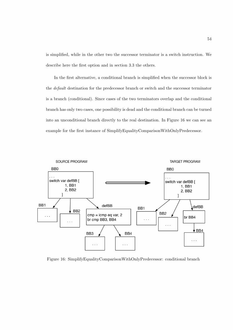
54

is simplified, while in the other two the successor terminator is a switch instruction. We

describe here the first option and in section 3.3 the others.

In the first alternative, a conditional branch is simplified when the successor block is

the default destination for the predecessor branch or switch and the successor terminator

is a branch (conditional). Since cases of the two terminators overlap and the conditional

branch has only two cases, one possibility is dead and the conditional branch can be turned

into an unconditional branch directly to the real destination. In Figure 16 we can see an

example for the first instance of SimplifyEqualityComparisonWithOnlyPredecessor.

Figure 16: SimplifyEqualityComparisonWithOnlyPredecessor: conditional branch

55

The witness for this simplification needs to take into account the old destination of the

successor block and the new one, since the simplification does not modify any other part

of the IR. The old destination, DefBB → getTerminator() → getSuccessor(cmp →

getPredicate() = ICMP EQ), is the successor of the branch that is not dead, while the

new destination, DefBB → getTerminator() → getOnlySuccessor(), is the only desti-

nation of the unconditional branch.

Here the complete witness (without including the declaration part):

(old.dest = DefBB → getTerminator() → getSuccessor(cmp → getPredicate() =

ICMP EQ)) ∧

(new.dest = DefBB → getTerminator()→ getOnlySuccessor()) ∧

(new.dest = old.dest)

• FoldValueComparisonIntoPredecessors:

The simplification tries to fold two blocks together if the current block and one of the

predecessor have an equality comparison as condition for the terminators (either a switch

or a branch). We can distinguish two main types of transformation: the successor (current

block) is the default destination of the predecessor or it is one of the cases handled. We

remind that the default case is the destination taken if the variable is not equal to any

of the values of the cases. If we are dealing with a conditional branch on an eq equality

comparison, the default case is the FalseSuccessor, otherwise, if the comparison is ne,

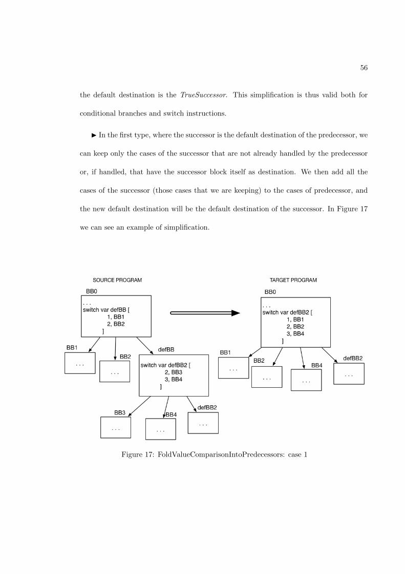
56

the default destination is the TrueSuccessor. This simplification is thus valid both for

conditional branches and switch instructions.

I In the first type, where the successor is the default destination of the predecessor, we

can keep only the cases of the successor that are not already handled by the predecessor

or, if handled, that have the successor block itself as destination. We then add all the

cases of the successor (those cases that we are keeping) to the cases of predecessor, and

the new default destination will be the default destination of the successor. In Figure 17

we can see an example of simplification.

Figure 17: FoldValueComparisonIntoPredecessors: case 1

57

The witness for the first type considers both the values of all the cases of the switch and

their destinations. The old switches and the new switch must be consistent, that means

that in the source part of the witness we assert the pairs case.value - case.destination of

the predecessor and the successor pairs not handled by the predecessor, instead, for the

target part, we assert all the cases of the new switch. If there are some new cases or if

some of the old cases is missing, the witness is not valid.

Here there is the source part witness. Notice that it is not actually used the forall

quantifier, but it is written here for conciseness and better clarity.

∀BB0.cases

((value = case.value)⇒ (destination = case.dest))

∀defBB.cases /∈ BB0.cases

((value = case.value)⇒ (destination = case.dest))

While for the target part we assert the same for the new switch:

∀BB0.cases

((value = case.value)⇒ (destination = case.dest))

I In the second type of transformation, where the successor is not the default

destination of the predecessor but one of the cases handled, we can have two alternatives

of simplification. In the first one, the successor handles the value of the predecessor which

58

is leading to the successor itself. We can perform jump threading, replacing the desti-

nation of the predecessor with the real destination of the successor case. In the second

alternative, the successor does not handle the value. We can perform again jump thread-

ing, but this time we replace the predecessor destination with the default destination of

the successor. The witnesses for both the alternatives are totally similar. In Figure 18 we

provide an example for the first one, and then its witness.

Figure 18: FoldValueComparisonIntoPredecessors: case 2.1

59

To generated the witness, we compute the real destination for all the cases of the switch.

If the new switch, after the transformation, has the right choices, then the witness is valid.

Here the source part:

∀BB0.cases

((value = case.value)⇒ (destination = case.realdest))

While the target part:

∀BB0.cases

((value = case.value)⇒ (destination = case.dest))

• SimplifyBranchOnICmpChain:

The current terminator instruction is a conditional branch on a condition determined

by a chain of equality comparison instructions. The chain is a conjunction of non-equality

comparisons, ne or a disjunction of equality comparisons, eq. All the comparisons are

against a constant integer value. The simplification transforms the chain into a switch

instruction. It is possible that one (no more than one) of the cases in the chain is an

extra case, not evaluating the same variable. We thus can insert a comparison on that

variable before the current block, and checking the new switch in the current block only

if the previous extra block comparison is true, if not-equal (ne), false, if equal (eq). In

Figure 19 we provide an example of simplification for a disjunction of eq comparisons.

60

Figure 19: SimplifyBranchOnICmpChain: disjunction of eq comparisons

The witness focuses on the condition of the old branch and on all the cases of the new

switch instruction.

The source part checks the two possible destinations against the condition of the branch:

(curBB.condition⇒ (destination = BB)) ∧

(¬(curBB.condition)⇒ (destination = defBB))

The target part loops on all the cases of the new switch. The push and pop Z3 statements

are used to check the witness against contrary conditions on the values of the cases:

61

∀curBB.cases

(push)

((var = case.value) ∧ (destination = case.realdest))

(pop)

• FoldBranchToCommonDest :

The optimization merges two blocks which have a common destination block, when

the current block (the successor) have no instructions, but only the comparison and the

conditional branch. One bonus instruction is allowed if used to compute the value needed

by the comparison (for instance, an addition to the variable that is then compared).

This transformation is used to simplify blocks whose terminator is a conditional or

unconditional branch. Here we explain the simplification on conditional branches, while

in section 3.4 we will describe the optimizations for unconditional branches.

The transformation recognizes a specific pattern in the CFG: the predecessor and the

successor blocks have both a conditional branch and have a common destination block.

This means that the predecessor has just the successor block and the common block as

destinations. The successor block, which is the block we are analyzing, has no additional

instructions beside the comparison and the branch. The merging is performed creating a

new condition for the predecessor branch and using logical operations. If the two blocks

share the TrueDestination, their two conditions are fused together into a disjunction,

since they are chances of the same condition, otherwise, if the shared destination is the

62

FalseDestination, the conditions are in a conjunction. In both configurations, the new

successors will be the common destination and the other destination of the successor

block. In Figure 20 we find the and configuration, while we already presented the or in

Figure 7.

Figure 20: FoldBranchToCommonDest: conjunction

The witness needs to take into account the conditions of the branches and the destination

blocks, in order to check the consistency of the transformation.

The source part:

((PredBB.condition ∧ SuccBB.condition)⇒

63

(destination = SuccBB.TrueDestination)) ∧

(¬(PredBB.condition ∧ SuccBB.condition)⇒

(destination = commonBB))

The target part:

(PredBB.condition⇒

(destination = PredBB.TrueDestination)) ∧

(¬PredBB.condition⇒

(destination = PredBB.TrueDestination))

• HoistThenElseCodeToIf :

Given a conditional branch that dominates its two successors, try to hoist the common

code of the successors into the predecessor. The conditional branch dominates the succes-

sors if it is their only predecessor and thus, there is no path in the graph that can reach

the blocks without visiting the predecessor block. The transformation does a very limited

instruction analysis to understand if the two successors share the same instructions. The

pass checks for identical instructions in identical order.

In Z3 there is no way to understand if two LLVM instructions are equal, or, with

the same result, it is impractical for our goal, since we should build a complex struc-

ture of functions and variables in Z3. Thus, we can check that the instructions hoisted

are identical from the LLVM-side and just assert true or false. In Z3: (assert-true) and

64

(assert-false).

If the successor blocks are empty or we hoisted all the instructions, there is the

possibility we hoist the common terminator instruction. After hoisting the terminator

instruction, we can remove the successor blocks. If there is a PHI node in the common

further successors blocks (they are all common since we are hoisting an identical termi-

nator instruction), update them with a select instruction in the predecessor block and

replace the PHI node values with the select instruction itself. In Figure 21 we provide an

example of the hoist of the terminator.

Figure 21: HoistThenElseCodeToIf: hoist of the terminator

65

The witness of the HoistThenElseCodeToIf takes into account the destination blocks and

the values in the PHI node. For the witness we used the construct ite: it is an if-then-else

structure which takes into consideration the second element if the condition (first element)

holds, otherwise it picks the third element, as explained in section 1.5.

The source part states the binding between the condition of the branch and the des-

tinations dominated:

(ite cond (block = BB1) (block = BB2))

The target part checks that the values assigned to the PHI node are correct and binds

the destinations to the values:

(ite (block = BB1) (value = val1) (value = val2)) ∧

(cond⇒ (value = val1)) ∧ (¬cond⇒ (value = val2))

• SpeculativelyExecuteBB :

This simplification tries to execute a block if it has just one predecessor and one

successor. It speculates on the execution of the block in order to flatten the CFG. The

transformation recognizes a specific pattern of the CFG: the predecessor branch can trans-

fer the control to two blocks, one of these has just one predecessor and is itself one of the

predecessors of the second block. If the first block has one instruction and that instruction

is not expensive, the method executes it anyway into the predecessor and puts a select

66

instruction to pick the right value, on the basis of the condition. In Figure 22 an example

of this type of simplification. We notice that the edges are not removed, but following

optimizations will simplify the CFG.

Figure 22: SpeculativelyExecuteBB: an example

The witness checks that the values assigned to the select instruction and the update of

the PHI node are correct.

67

The source part of the witness checks the values in the phi node:

(cond⇒ (var = phi.value.for(BB1))) ∧

(¬cond⇒ (var = phi.value.for(BB0)))

While the target part checks the values in the select instruction:

(cond⇒ (var = select.T rueV alue)) ∧

(¬cond⇒ (var = select.FalseV alue))

• FoldCondBranchOnPHI :

If we have a conditional branch whose condition is a variable defined by a PHI node

in the same block, we can thread the edges for the phi entries that assign a constant

value directly to their real destinations. A branch on a constant value is a branch taken,

unless the constant is zero. The simplification changes the destination block of all those

predecessors of the PHI node which correspond to a constant entry. All the instructions

of the PHI node basic block are cloned into a new block that will be the new destination

of the predecessor branch. This proceeding, the simplification does not have to be smart

reasoning on the following PHI nodes, it is enough to update them.

In Figure 23 we provide an example: the predecessor now transfers the control directly

to the real destination.

The witness checks the predecessor block and its real destination, taking into account

also if the new block branches to the right destination. The cloning of the instructions is

68

Figure 23: FoldCondBranchOnPHI: an example

checked LLVM-side.

Here the source part states the predecessor name and the right destination:

(PredBlock = PredBB1)⇒ (SuccBlock = BB.TrueSuccessor)

The target part checks that the predecessor block branches to the new block and this

one branches to the old destination:

69

(PredBlock = NewBB.Predecessor) ∧ (SuccBlock = NewBB.Successor)

• SimplifyCondBranchToCondBranch:

This simplification tries to simplify the conditional branch of the successor block of

another block with a conditional branch. If the second conditional branch is on the same

condition as the first terminator, the simplification is trivial, and the successor has just

one predecessor. The optimization knows that the second branch will be surely taken so

it can turn the branch into a branch on a constant that will be simplified in following

transformations.

If the successor has multiple predecessors, the pass cannot be always sure about

the outcome of the condition of the branch, because we may be at the current block

coming from a block different than the predecessor, whose condition is the same as our

conditional branch. The simplification inserts in the successor a PHI node whose values

are constants, if we know the outcome of the conditions, or, keeping symbolic, the values

are the conditions of the predecessors branches. The branch will jump on the basis of

the value assigned to the condition by the PHI node. In Figure 24 an example for this

simplification: BB branch is on the same condition as PredBB1 and PredBB2, so in the

PHI node there is a constant, because the branch is taken; while for PredBB3 it is kept

symbolic with cmp2.

The witness takes into account the conditions of the predecessors and the destination

blocks. The source part asserts that if the predecessor condition holds, and the condition

70

Figure 24: SimplifyCondBranchToCondBranch: an example

is not the same as the successor one, then the final destination is either the TrueDestina-

tion or the FalseDestination of the successor branch. Instead, if the condition is the same

for both the branches, the final destination is known and we can assert it. The target part

of the witness assert the same but using the condition values of the new PHI node inserted.

The source part:

∀PredBB

if(same condition) :

(PredBB.cond⇒ (Succ = BB.Succ(¬PredBB.cond)))

else if(different condition) :

(PredBB.cond⇒ ((Succ = BB.Succ(0)) ∨ (Succ = BB.Succ(1))))

71

The target part:

∀PHI.entries

if(PHI.value is constant) :

(Succ = BB.Succ(¬PHI.value))

else :

(PHI.value⇒ ((Succ = BB.Succ(0)) ∨ (Succ = BB.Succ(1))))

The simplification can handle also the case where the conditions of the two branches

are different but the two blocks have a common successor. In this case the transforma-

tion is totally similar to the optimization performed by the FoldBranchToCommonDest

method.

In the next section (3.3) we will analyze the simplifications of switch instructions and in the

remaining part of the chapter we will describe the other optimizations of the SimplifyCFG.

3.3 Switch Instructions

This section will provide detailed information about the simplifications involving switch in-

structions. We will go through the optimizations performed and their witness relations. As

explained in section 1.4.1, the switch instruction is a terminator which performs an equality

comparison on a variable and, on the basis of its value, transfers the flow of control to different

blocks, depending on different cases. If none of the cases matches, the control is transferred to

72

a default destination.

• SimplifyEqualityComparisonWithOnlyPredecessor :

This simplification performs optimizations on both conditional branches and switch

instructions. We have seen in section 3.2 the analysis of conditional branch transfor-

mations. Here we analyze transformations of switch instructions. We remind that the

transformation simplifies blocks with only one predecessor in which the terminator is an

integer equality comparison on the same value of the terminator we are studying. The

cases of the comparison instructions must overlap in order to perform the optimizations.

As usual, we will call successor the current block we are analyzing, and predecessor its

only predecessor. Here we describe two alternatives of the simplification, involving switch

instructions.

I In the first alternative, predecessor and successor have both a switch instruc-

tion as terminator and the successor block is the default destination of the predecessor

switch. Since cases overlap, the transformation removes from the successor all the cases

already handled by the predecessor. This is a trivial configuration and the witness just

assert true or false after we have checked the consistency of the operations LLVM-side.

I The second alternative is more interesting and we will provide an example and

the typical witness. We have two switch terminators and the successor is one of the

73

destinations of the predecessor. We thus know the value of the variable coming to the

current block.If the successor switch handles that value, we redirect the jump to the real

destination, otherwise the following block is the default of the second switch. In both

cases, an unconditional branch is placed removing the switch instruction.

In Figure 25 we show an example of the second alternative of SimplifyEquality-

ComparisonWithOnlyPredecessor.

Figure 25: SimplifyEqualityComparisonWithOnlyPredecessor: case 1

74

The witness needs to check just the amount of code has been transformed. The source

part states which is the destination for that value in the second switch instruction, while

the target part checks that the destination of the new unconditional branch is the same

as the previous block just asserted.

Here the complete witness (without the declaration part):

(old.dest = BB2.getSuccForV alue(2)) ∧

(new.dest = BB2.getOnlySuccessor()) ∧

(new.dest = old.dest)

• SimplifySwitchOnSelect :

The optimization replaces a switch on a select result with a branch, conditional if the

two destinations are different. A select is an instruction which chooses between two values

on the basis of a condition. For this simplification the values of the select are constant

values, since otherwise they cannot be cases of the switch. There are actually three alter-

natives. If the destinations are equal, replace the switch with an unconditional branch. If

the destinations are unreachable, replace the terminator with an unreachable instruction.

In LLVM-IR, an unreachable instruction is an instruction without any semantics, it is a

marker to enable further optimizations. The third alternative is the most interesting: the

two destinations are different and the transformation replaces the switch instruction with

an unconditional branch.

75

We want to notice that the default destination of the switch instruction can never be

reach, since the select instruction always returns one of the two value cases. In Figure 26

an example of SimplifySwitchOnSelect.

Figure 26: SimplifySwitchOnSelect: example for conditional branch

The witness checks that the destinations of the new conditional branch are consistent

with the cases of the switch instruction and the condition of the select instruction.

The source part of the witness:

76

(select.cond⇒ (dest = BB.getDestForV alue(val1))) ∧

(¬select.cond⇒ (dest = BB.getDestForV alue(val2)))

The target part:

(br.cond⇒ (dest = BB.TrueDest)) ∧

(¬br.cond⇒ (dest = BB.FalseDest))

• FoldValueComparisonIntoPredecessors:

This simplification folds to blocks together if both their terminators have an equality

comparison as conditions, and the two blocks are one the predecessor of the other. This

optimization has been already described in section 3.2, since it simplifies also conditional

branches. An example is provided in Figure 17.

• TurnSwitchRangeIntoICmp:

If the cases of a switch instruction are integers which belong to a range interval, turn

the switch into a comparison and a branch. If the range does not start from zero, add the

initial subtraction of the offset. This is instruction replacement: the expensive switch is

turned into simple integer operations. Obviously, to be able to transform the switch into

a comparison, all the cases must have the same block as destination. In Figure 27 we have

an example of simplification. The switch in BB has four cases all directing to the basic

block destBB. The values are in the range 6 ≤ case.value ≤ 10. The offset is then 6 while

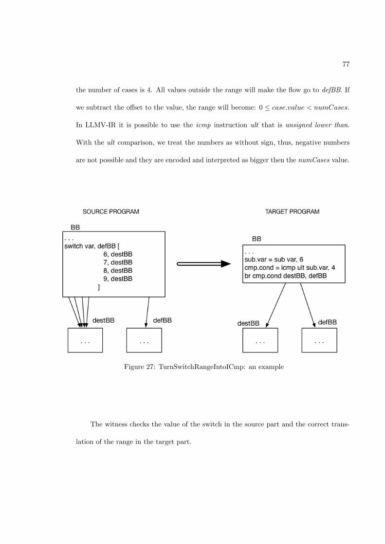
77

the number of cases is 4. All values outside the range will make the flow go to defBB. If

we subtract the offset to the value, the range will become: 0 ≤ case.value < numCases.

In LLMV-IR it is possible to use the icmp instruction ult that is unsigned lower than.

With the ult comparison, we treat the numbers as without sign, thus, negative numbers

are not possible and they are encoded and interpreted as bigger then the numCases value.

Figure 27: TurnSwitchRangeIntoICmp: an example

The witness checks the value of the switch in the source part and the correct trans-

lation of the range in the target part.

78

Here the source part:

{ite [(value = case1.value) ∨ (value = case2.value) ∨

(value = case3.value) ∨ (value = case4.value)]

(dest = case.dest) (dest = default.dest)}

Here the target part:

[(value− offset) ≥ 0] ∧ [(value− offset) < numCases)] ∧ (dest = br.T rueDest)

∧

¬{(value− offset) ≥ 0] ∧ [(value− offset) < numCases]} ∧ (dest = br.FalseDest)

• EliminateDeadSwitchCases:

This simplification removes all the cases of the switch instruction we are sure

cannot be taken. This can happen when we already know the value of the variable

we are switching on. The simplification just removes the dead cases, without removing

basic blocks or replacing instructions. Those optimizations will be performed by further

simplifications on the resulting target code. In Figure 28 we provide an example of

EliminateDeadSwitchCases.

The witness takes into consideration the values and the destinations of the switch

cases. The source part asserts the cases of the switch before the transformation, while the

target part asserts the cases of the target code. We need to notice that is possible that

79

Figure 28: EliminateDeadSwitchCases: an example

all the cases are dead; in this case the only possible destination block is the default one.

The source part of the witness:

∀switch.cases

(value = case.value)⇒ (destination = case.dest)

∧

(value /∈ switch.cases.value⇒ (destination = defBB)

The target part:

80

if(numAliveCases > 0)

∀switch.cases

(value = case.values) ∧ (destination = case.dest)

if(onlyDefaultCaseLeft)

(destination = defBB)

• SwitchToSelect :

If the switch instruction is used to initialize a value in the PHI node of a common

successor block with two different constant values, the simplification replaces the switch

with a select instruction and an unconditional branch. A switch is used to initialize a

value if its block dominates two blocks whose common successor has a PHI node. In

the PHI node will be chosen a value depending on the incoming block. It is possible to

replace the switch and remove the blocks using a select instruction that will choose the

right value on the basis of a condition created from a switch instruction with two cases.

The switch checks if a variable is equal to two different values. The resulting condition is

a combination of select instructions as shown in Figure 29. We need to notice that if the

variable used in the switch is a constant whose value is known, the select instruction is

useless and not inserted. After the transformation, the PHI node will be reachable only

from the switch parent block and the value resulting from the select is replaced in the

PHI node entry for the block. All other entries of the PHI node become useless.

81

Figure 29: SwitchToSelect: an example

The witness takes into account the value of PHI node and the original values in the switch

cases.

For the source part:

∀entry.Cases

(value = case.value) ∧ (variable = phi.variableForBlock(case.dest))

For the target part:

(push)

82

(value = phi.variableForBlock(entry).T rueV alue)⇒ (value = variable)

(pop)

(push)

(value = phi.variableForBlock(entry).FalseV alue)⇒ (value = variable)

(pop)

• ForwardSwitchConditionToPHI :

If a block with a switch instruction as terminator dominates a PHI node, this simpli-

fication tries to forward the switch condition (the variable being compared) to the PHI

node entries. This may have, as consequence, the deletion of some switch cases and their

destination blocks. The optimization can forward the variable if in the PHI node entry,

for the case destination, the value returned is equal to the value of the case. It is possible

to directly put that variable as the value returned by the PHI instruction, and remove

the switch case and the block. In Figure 30 we provide an example of ForwardSwitch-

ConditionToPHI.

The witness for this simplification takes into account the variable of the switch and the

PHI node, together with the destination blocks.

Here the source part:

∀BB.Cases

(var = phi.var) ∧ (var = phi.V arForBlock(case.dest)) ∧ (dest = case.dest)

83

Figure 30: ForwardSwitchConditionToPHI: an example

While the target part is:

∀phi.Entries

(phi.var = phi.value) ∧ (dest = phi.incomingBlock)

84

3.4 Unconditional Branches

We provide in this section detailed information of the simplifications of unconditional branches.

We will describe the optimizations performed and their typical witnesses. As explained in sec-

tion 1.4.1 a branch is a terminator instruction which transfers the flow of control to the next

block in the CFG path. Branches can be conditional, if they have two different destinations

and transfer the control on the basis of the outcome of a condition, or can be unconditional,

if they transfer always the control to a predetermined basic block. An unconditional branch

takes only one argument that is the basic block to which the control is passed. In Listing 1.6

we have an example of both kinds of branches.

• SinkThenElseCodeToEnd :

This simplification recognizes the precise CFG patter where two blocks with uncondi-

tional branches have the same successor. The method sinks into the common destination

all the instructions shared by its two only predecessors. The matching of the instruc-

tion is trivial, they need to be identical or at most one operand can be different. If the

operand is different a PHI node is added to the successor to discriminate the right value.

In Figure 31 an example of SinkThenElseCodeToEnd.

In the same way as for the simplification HoistThenElseCodeToIf, it is not possible to

check in Z3 if two instructions are identical. Thus, we checked the conditions for a correct

transformation directly within the LLVM code. The resulting witness sent to Z3 will be an

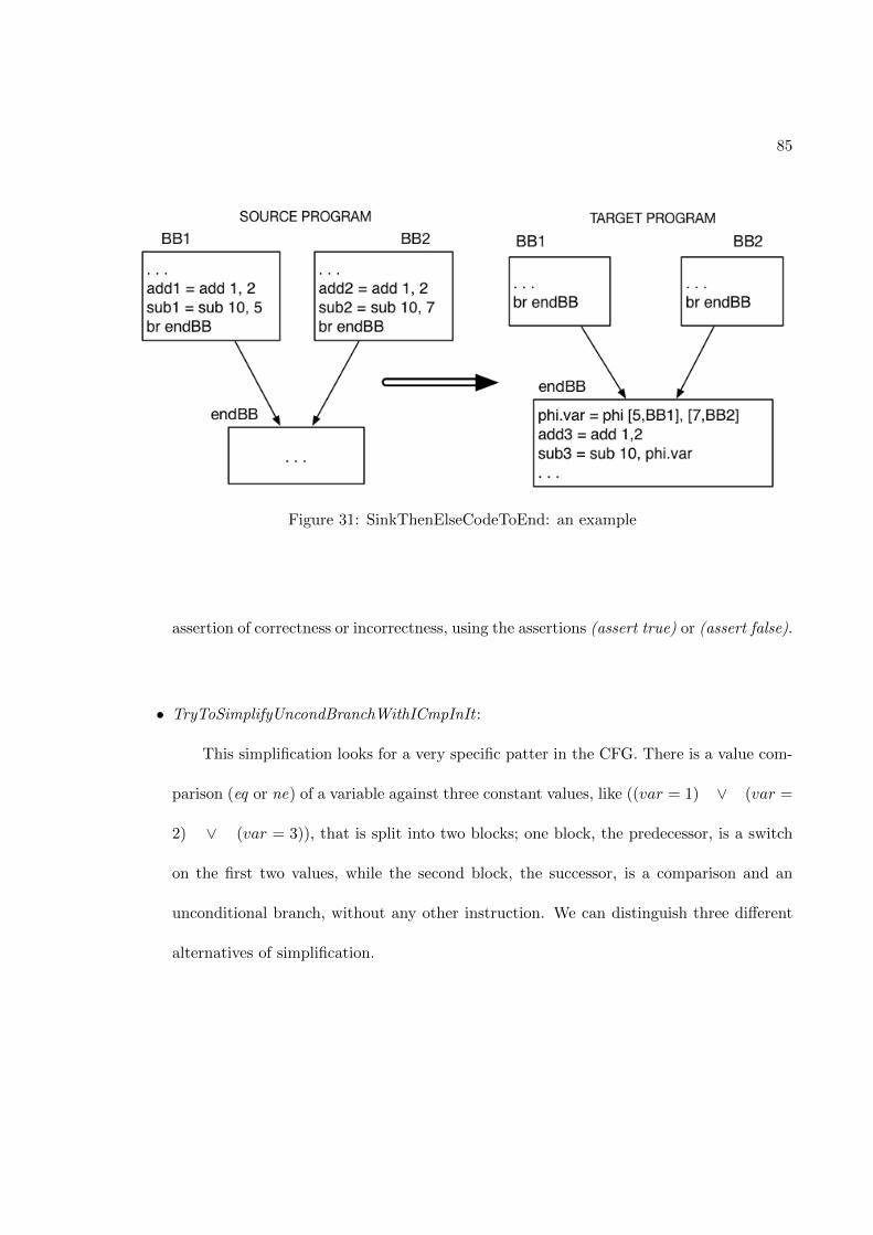
85

Figure 31: SinkThenElseCodeToEnd: an example

assertion of correctness or incorrectness, using the assertions (assert true) or (assert false).

• TryToSimplifyUncondBranchWithICmpInIt :

This simplification looks for a very specific patter in the CFG. There is a value com-

parison (eq or ne) of a variable against three constant values, like ((var = 1) ∨ (var =

2) ∨ (var = 3)), that is split into two blocks; one block, the predecessor, is a switch

on the first two values, while the second block, the successor, is a comparison and an

unconditional branch, without any other instruction. We can distinguish three different

alternatives of simplification.

86

I In the first alternative, the value comparison in the successor is one of the

values already checked by the switch in the predecessor. We already know the outcome

of the successor comparison and we can remove it, replacing the result in all its uses.

In the second and third alternatives the successor block is the default block of the prede-

cessor.

I In the second one, the constant we are comparing to the variable is on of the

cases of the predecessor switch: the comparison is useless and can be removed, replacing

it with true or false.

I In the third one, we need to add a new case to the switch instruction whose

destination block is a new block. In the PHI node that is the convergence block of the

switch cases we need to add an entry for the new block and set its value to true, if the com-

parison was of equality (eq), or false otherwise. This is the most interesting alternative

and we provide an example in Figure 32 and then its typical witness relation.

The witness needs to take into account the new value of the case added and the new entry

in the PHI node.

The source part of the witness:

(var 6= defBB.icmp.value)⇒ (val = true) in the case of inequality;

87

Figure 32: TryToSimplifyUncondBranchWithICmpInIt: case 3

(var = defBB.icmp.value)⇒ (val = false) in the case of equality.

The target part:

(var = newCase.value) ∧ (val = phi.valueForBlock(defBB))

• FoldBranchToCommonDest :

This transformation simplifies two basic blocks if one is the predecessor of the other

one, which terminates with an unconditional branch to a basic block that is the second

destination of the predecessor conditional branch. This is a correct transformation also if

88

in the successor block is present a conditional branch; we described this situation in the

FoldBranchToCommonDest simplification for conditional branches in section 3.2.

For the unconditional branch simplification, the successor block can have many

instructions, which will be removed if they already appear identical in the predecessor.

The resulting successor is then composed of only the comparison instruction and the

unconditional branch to the common destination. Another condition for the simplification

is that the PHI node in the common successor handles boolean values, that is, conditions.

We can now distinguish two different situations: the successor is the TrueDestination

or the FalseDestination of the predecessor block. In both alternatives, the simplification

removes the successor block and replaces the condition in the common destination PHI

node for the predecessor block. The condition replaced is different for the two situations.

I If the successor is the TrueDestination the condition in the PHI node will be:

(Pred.cond ∧ phi.valueForBlock(Succ)) ∨

(¬Pred.cond ∧ phi.valueForBlock(Pred))

If the Pred.cond is true, then the right value is the value given by the successor:

phi.valueForBlock(Succ)

Otherwise, if Pred.cond is false, then the right value is the value for the predecessor:

phi.valueForBlock(Pred)

I If the successor is the FalseDestination the condition in the PHI node will be:

89

(Pred.cond ∧ phi.valueForBlock(Pred)) ∨

(¬Pred.cond ∧ phi.valueForBlock(Succ))

If the Pred.cond is true, then the right value is the value given by the predecessor:

phi.valueForBlock(Pred)

Otherwise, if Pred.cond is false, then the right value is the value for the successor:

phi.valueForBlock(Succ)

In Figure 33 we provide an example of the configuration where the successor is the

true destination of the predecessor. We notice how the not condition is modeled as a xor

with a true value.

The witness needs first to bind the conditions of the branches with the values in the PHI

node. Then, it checks that, in the resulting PHI node, the value, which is the condition

of the merged block, is consistent. We are witnessing both the right replacement of the

PHI value and the right composition of the condition.

The source part:

Pred.cond⇒ (value = phi.valueForBlock(Succ)) ∧

¬Pred.cond⇒ (value = phi.valueForBlock(Pred))

The target part:

value = phi.valueForBlock(Pred)

90

Figure 33: FoldBranchToCommonDest: unconditional branches, case 1

3.5 Other Simplifications

In this section we will provide information about CFG simplifications that are not grouped

into any class of instructions.

• SimplifyCondBranchToTwoReturns:

If we have a conditional branch directing the flow towards two blocks with a return

91

instruction as terminator, the simplifications tries to merge them into the predecessor,

replacing the branch wit a return. If the returning values disagree, a select with the

condition of the old branch is inserted. The two returning blocks must not have any

additional instruction other than the return and possible initial PHI nodes.

When the two returns are void the simplification is trivial: it is sufficient to change

the conditional branch into a void return instruction. The same solution is applied in case

the two values are equal. If instead the two values differ, a select instruction is inserted

with the condition of the branch and the branch is replaced with a return instruction

whose value is the one given by the select. In Figure 34 we provide an example.

Figure 34: SimplifyCondBranchToTwoReturns: an example

92

The witness takes into account the values of the return instructions before the sim-

plification, and the condition and values of the select instruction after the simplification.

The source part:

(BB.cond⇒ (value = BB1.returnV alue)) ∧

(¬BB.cond⇒ (value = BB2.returnV alue))

The target part:

(BB.selectCond⇒ (value = BB.selectTrueV alue)) ∧

(¬BB.selectCond⇒ (value = BB.selectFalseV alue))

• SimplifyIndirectBrOnSelect :

An IndirectBranch instruction is a branch to a label inside the current function. This

instruction takes as argument the address of the destination of the jump. If the address

is the result of a select instruction, it is possible to change the indirect branch with a

conditional branch whose condition is the condition of the select, while the destinations

are the two possible address values. This simplification is actually already described in

section 3.3, when describing the transformation SimplifySwitchOnSelect. Both the trans-

formations retrieve the condition of the select instructions and the possible destination

blocks, then call a function whose task is to simplify a terminator replacing it with a

conditional branch on a certain condition towards to specified basic blocks. The name of

93

this function is indeed SimplifyTerminatorOnSelect.

• FoldTwoEntryPHINode:

This simplification tries to simplify a PHI node that has only two entries. The

transformation searches for the CFG pattern of an if statement : a block can branch

to two different destinations depending on a condition, and those destinations have a

common successor with the two-entry PHI node.

The optimization hoists all the instructions of the two destinations blocks into the pre-

decessor and then replaces the PHI node with a select instruction. The select instruction

picks the right value on the basis of the condition of the branch in the predecessor, which

is removed in favor of an unconditional branch to the common destination. Figure 35

shows an example of transformation.

The witness checks that the condition of the conditional branch is correctly used for the

select instruction and the two values are the ones belonging to the entries of the PHI node.

The source part:

(BB.cond⇒ (value = phi.valueForBlock(BB1))) ∧

(¬BB.cond⇒ (value = phi.valueForBlock(BB2)))

The target part:

(select.cond⇒ (value = select.T rueV alue)) ∧

94

Figure 35: FoldTwoEntryPHINode: an example

(¬select.cond⇒ (value = select.FalseV alue))

• MergeEmptyReturnBlocks:

This simplification merges all the empty return blocks of the whole function. An empty

return block has only the ret instruction and nothing else other than a PHI node that is

the returning value. If the blocks return the same value (or no value) the simplification is

trivial, it removes all duplicates and keeps just one block, redirecting all the predecessor

to this block. If the blocks have different returning values, the transformation inserts

a PHI node which will be updated every time a new empty returning block is found.

95

All returning blocks will branch unconditionally to this returning PHI node. This last

situation is the most interesting one and we provide an example in Figure 36.

Figure 36: MergeEmptyReturnBlocks: an example

The witness checks that the values in the entries of the PHI node are the values returned

by the returning blocks. All the values must be associated to the right incoming block.

The source part:

((block = BB1)⇒ (value = BB1.return.value)) ∧

96

((block = BB2)⇒ (value = BB2.return.value))

The target part:

∀BB2.predecessors

((block = pred) ∧ (value = phi.getV alueForBlock(pred))) ∧

((block = BB1) ∧ (value = phi.getV alueForBlock(BB1))

After the description of the simplifications implemented in the SimplifyCFG pass, in chapter

4 we will show how we tested our witness generation procedure, the benchmarks used and the

results obtained.

CHAPTER 4

BENCHMARKING AND RESULTS

In this chapter we describe the implementation process, provide insight on the methods

used to test the witnessing procedure and analyze our benchmarks.

4.1 Testing the Witnessing Procedure

The LLVM back-end is composed of different optimization passes performing different trans-

formations of the code. Each of the passes is further divided into methods covering different

cases of a specific optimization. This modular structure is repeated until the finest grain of

detail. Consequently, testing the witnessing procedure on a single simplification is difficult. We

need to isolate the method we are augmenting, without any other optimization involved, and

to test every case covered by the simplification.

Augmenting the pass with the procedure requires a complete knowledge of the optimization

code. We can leverage this by designing a source program able to trigger the specific optimiza-

tion we are analyzing. As we already described in the first chapters of this thesis, the source

code, implemented in a language of the C-family, is translated by CLANG into the LLVM

IR-language and submitted to the compiler optimizer. The source program can be designed

and implemented in the high level programming language or directly modifying the IR code.

Both approaches have been used to test the witnessing procedure.

97

98

• C-Family Programming Language:

We have designed snippets of C code, to be translated into IR, with specific structure

and instructions that enable the simplifications. A single optimization has different sub-

cases that need to be tested and are triggered by particular configurations of the CFG.

• Intermediate Representation:

Some simplifications do not perform optimizations directly on the IR code, but rather

simplify CFG patterns that are the results of previous transformations. It is not possible

in this case to design a source from the high level programming language. We created IR

snippets, reproducing the particular CFG patterns treated by the code.

Many optimization cases overlap, and the same CFG pattern can be transformed in different

ways. Moreover, some transformations can enable or disable each others. For these reasons, to

isolate an optimization, sometimes we commented the other optimizations, making the inter-

esting one the only possible transformation available.

Another important aspect of the development process is to have an immediate feedback on

the type and number of simplifications performed during a single execution of the compiler.

We already described in section 2.2 how we instrumented the SimplifyCFG code with STATIS-

TIC variables that profile the behavior of the code, informing on the simplifications performed.

To know exactly which simplification is being performed, we print to console an informative

message and insert an echo command inside the witnesses, to have a feedback also in the

99

verification phase of the formula. All simplifications are numbered with the current value of

the proper statistic variable. In Listing 4.1 we show an example of console output.

1 ####### FoldValueComparisonIntoPredecessors number: 0_1

2 ####### HoistThenElseCodeToIf number: 0

3 ####### HoistThenElseCodeToIf number: 1

4 ####### FoldBranchToCommonDest number: 5

5 ####### FoldValueComparisonIntoPredecessors number: 1_1

6 ####### FoldBranchToCommonDest number: 1

7 ####### FoldCondBranchOnPHI number: 0_0_0

8 ####### FoldTwoEntryPHINode number: 2

9 ####### SpeculativelyExecuteBB number: 0_1

10 ####### SinkThenElseCodeToEnd number: 2

11 ####### EliminateDeadSwitchCases number: 4

12 ####### TurnSwitchRangeIntoICmp number: 3

13 ####### SimplifyEqualityComparisonWithOnlyPredecessor number: 0

Listing 4.1: Console output

In the next section (4.2) we will describe how we tested the witnessing procedure and the

SimplifyCFG pass, using benchmarks to understand the needs of our generator and to test the

correctness of both the pass and the procedure.

4.2 Benchmarks

Benchmarks have been used throughout the development process to both testing the witness-

ing procedure and the SimplifyCFG pass transformations. Along with the custom C-language

and IR-language snippets, benchmarks were useful to make the optimizations run in a real-

world case, with configurations that are difficult to predict at design-time. Benchmarks used

are single-file C-programs, submitted as input to the simplification pass. The witness rela-

100

tions extracted from the transformations performed have been used to check the pass and the

procedure itself.

We can divide the benchmarks used into two different categories, on the basis of the size of

the files. The first category is composed of small C-programs, useful to have a fast feedback

of the level of correctness of the procedure implemented. These programs have been functional

to discover errors in the Z3 syntax of the witnesses. In Table I we provide the benchmarks

together with the number of lines of code and the number of calls to the SimplifyCFG pass,

as measured by the statistic variables. We provide also aggregate data about the number of

simplifications performed.

TABLE I: BENCHMARKS, FIRST GROUP

Benchmark LOC n simplifications n calls to SimplifyCFG

GC10 113 16 81DIJKSTRA 182 15 87MxM 790 65 271LINPACK 1197 103 379SUSAN 2121 269 1318

The second group of benchmarks is composed of three large single-file C-programs. These

have been useful, other than to check deeply the Z3 syntax of the witnesses, to test the witness-

ing procedure against unpredicted patterns and contexts generated by the SimplifyCFG pass

101

with a long sequence of different optimizations. In Table II we provide information about the

benchmarks of this group and the number of simplifications performed on their code.

TABLE II: BENCHMARKS, SECOND GROUP

Benchmark LOC n simplifications n calls to SimplifyCFG

BZIP2 7,084 1,238 6,591GZIP 8,607 996 5,136OGGENC 58,408 2,942 13,092

4.3 Results

In this section we describe with deeper details the outputs of the SimplifyCFG pass when

compiling the benchmarks introduced in section 4.2.

A run of the compiler is correct when Z3 SMT-Solver returns SAT as result of the verifica-

tion of the formulas describing the witness relations. We run the SimplifyCFG pass using the

benchmarks as input and after the execution of the mem2reg pass, which promotes memory

accesses to register accesses, removing load and store instructions for allocation of registers.

The mem2reg pass also transform the IR-code into complete SSA form.

The benchmarks, together with the snippets of code created to test the witnessing procedure,

102

both in C language and in IR language, can be used to test the correctness of the Simplify-

CFG pass. None of our benchmarks revealed errors of the SimplifyCFG pass. Here, as in all

the Translation Validation work, one cannot conclude the correctness of the pass, but only its

correctness for the transformations that were checked.

Table III shows an example of output of LLVM after a compilation (example for bzip2 ). Here

we can see information about the single simplifications performed. Values for lines like Number

of conditional branches simplified or Number of switch instructions simplified provide overall

data about all simplifications performed inside the specified category.

TABLE III: BZIP2 SIMPLIFICATIONS

Simplification n occurrenciesSimplifyCondBranchToTwoReturns 1Number of times unreachable blocks are removed 86Number of UNconditional branches simplified 705Number of calls to SimplifyCFG 6591Number of conditional branches simplified 136Number of return instructions simplified 1Number of switch instructions simplified 5FoldBranchToCommonDest 70FoldCondBranchOnPHI 2FoldValueComparisonIntoPredecessors 18HoistThenElseCodeToIf 26SimplifyEqualityComparisonWithOnlyPredecessor 2SpeculativelyExecuteBB 18SinkThenElseCodeToEnd 7TryToSimplifyUncondBranchFromEmptyBlock 698Number of blocks into predecessor merged 167Number of dead blocks deleted 119Number of terminator instruction folded 6Number of two entry PHI nodes merged 13

103

In Appendix A we present the complete list of simplifications performed by the SimplifyCFG

pass while Appendix B is the list of all the simplifications triggered by the benchmarks used.

CHAPTER 5

CONCLUSION AND FUTURE WORK

Proving the correctness of a program transformation, and specifically, of a compiler opti-

mization, is a long-standing research problem.

In this work we showed that it is feasible to augment SimplifyCFG with a witness generator.

The witnesses have been submitted to the SMT-Solver Z3. We tested our implementation to

validate the correctness of both the witness generator and the compiler optimizations.

The SimplifyCFG is a good pass to validate through the witnessing methodology, since we

do not except to have bugs in the code. In fact, to debug the implementation, we viewed any

reported bug as an indication of an error in our procedure, rather than in the tested program.

Moreover, the SimplifyCFG, as indicated by LLVM profiling statistic variables, is one of the

most frequent executed pass.

This work is a further step towards the implementation of a witnessing compiler. We aim

to extend the methodology to all the passes of LLVM.

For the SimplifyCFG pass, the next step is upgrading the implementation in order to elim-

inate the use of files as inputs to Z3, in favor of the Z3 API to handle many different witness

relations for different passes, in a complete and maintainable framework.

104

105

As mathematical formulas, the witnesses (and also the transformations) can be improved

by introducing further information provided by external static analysis tools. Knowing the

domain and the bounds of a variable values, can be functional to the simplifications and the

construction of the witnesses, improving the overall effectiveness of the optimization and the

verification procedure.

APPENDICES

106

107

Appendix A

SIMPLIFICATIONS OF THE SimplifyCFG

Here we provide a list of all the simplifications performed by the SimplifyCFG pass.

TABLE IV: SIMPLIFICATIONS OF THE SIMPLIFY CFG PASS

Group Simplifications

Conditional Branches

SimplifyEqualityComparisonWithOnlyPredecessorFoldValueComparisonIntoPredecessorsSimplifyBranchOnICmpChainSpeculativelyExecuteBBFoldCondBranchOnPHISimplifyCondBranchToCondBranch

Switch Instructions

SimplifyEqualityComparisonWithOnlyPredecessorSimplifySwitchOnSelectFoldValueComparisonIntoPredecessorsTurnSwitchRangeIntoICmpEliminateDeadSwitchCasesSwitchToSelectForwardSwitchConditionToPHISwitchToLookupTable

Unconditional Branches

SinkThenElseCodeToEndTryToSimplifyUncondBranchFromEmptyBlockTryToSimplifyUncondBranchWithICmpInItFoldBranchToCommonDest

Other Simplifications

FoldReturnIntoUncondBranchSimplifyCondBranchToTwoReturnsSimplifyResumeSimplifyUnreachableSimplifyIndirectBrFoldTwoEntryPHINodeMergeBlockIntoPredecessorEliminateDuplicatePHINodesConstantFoldTerminatorDeleteDeadBlockRemoveUndefIntroducingPredecessorRemoveUnreachableBlocksMergeEmptyReturnBlocks

108

Appendix B

SIMPLIFICATIONS IN BENCHMARKS

Here we provide tables with details of the simplifications executed by the benchmarks used.

TABLE V: GC10 SIMPLIFICATIONS

Simplification n occurrencies

Number of times unreachable blocks are removed 4Number of UNconditional branches simplified 4Number of calls to SimplifyCFG 81Number of conditional branches simplified 1HoistThenElseCodeToIf 1TryToSimplifyUncondBranchFromEmptyBlock 4Number of blocks into predecessor merged 7

TABLE VI: DIJKSTRA SIMPLIFICATIONS

Simplification n occurrencies

Number of times unreachable blocks are removed 4Number of UNconditional branches simplified 7Number of calls to SimplifyCFG 87Number of conditional branches simplified 1HoistThenElseCodeToIf 1TryToSimplifyUncondBranchFromEmptyBlock 7Number of blocks into predecessor merged 3

109

Appendix B (continued)

TABLE VII: MXM SIMPLIFICATIONS

Simplification n occurrencies

Number of times unreachable blocks are removed 8Number of UNconditional branches simplified 44Number of calls to SimplifyCFG 271TryToSimplifyUncondBranchFromEmptyBlock 44Number of blocks into predecessor merged 13

TABLE VIII: LINPACK SIMPLIFICATIONS

Simplification n occurrencies

Number of times unreachable blocks are removed 10Number of UNconditional branches simplified 54Number of calls to SimplifyCFG 379Number of conditional branches simplified 6FoldBranchToCommonDest 4HoistThenElseCodeToIf 2SinkThenElseCodeToEnd 1TryToSimplifyUncondBranchFromEmptyBlock 53Number of blocks into predecessor merged 25Number of dead blocks deleted 7Number of two entry PHI nodes merged 1

110

Appendix B (continued)

TABLE IX: SUSAN SIMPLIFICATIONS

Simplification n occurrencies

Number of times unreachable blocks are removed 18Number of UNconditional branches simplified 175Number of calls to SimplifyCFG 1318Number of conditional branches simplified 28FoldBranchToCommonDest 4FoldValueComparisonIntoPredecessors 2HoistThenElseCodeToIf 17SimplifyEqualityComparisonWithOnlyPredecessor 2SpeculativelyExecuteBB 3SinkThenElseCodeToEnd 7TryToSimplifyUncondBranchFromEmptyBlock 168Number of blocks into predecessor merged 22Number of dead blocks deleted 21Number of two entry PHI nodes merged 5

TABLE X: BZIP2 SIMPLIFICATIONS

Simplification n occurrencies

SimplifyCondBranchToTwoReturns 1Number of times unreachable blocks are removed 86Number of UNconditional branches simplified 705Number of calls to SimplifyCFG 6591Number of conditional branches simplified 136Number of return instructions simplified 1Number of switch instructions simplified 5FoldBranchToCommonDest 70FoldCondBranchOnPHI 2FoldValueComparisonIntoPredecessors 18HoistThenElseCodeToIf 26SimplifyEqualityComparisonWithOnlyPredecessor 2SpeculativelyExecuteBB 18SinkThenElseCodeToEnd 7TryToSimplifyUncondBranchFromEmptyBlock 698Number of blocks into predecessor merged 167Number of dead blocks deleted 119Number of terminator instruction folded 6Number of two entry PHI nodes merged 13

111

Appendix B (continued)

TABLE XI: GZIP SIMPLIFICATIONS

Simplification n occurrencies

FoldValueComparisonIntoPredecessorsSwitch 1Number of times unreachable blocks are removed 87Number of UNconditional branches simplified 477Number of calls to SimplifyCFG 5136Number of conditional branches simplified 157Number of switch instructions simplified 1FoldBranchToCommonDest 65FoldCondBranchOnPHI 5FoldValueComparisonIntoPredecessors 14HoistThenElseCodeToIf 51SpeculativelyExecuteBB 22SinkThenElseCodeToEnd 7TryToSimplifyUncondBranchFromEmptyBlock 470Number of blocks into predecessor merged 130Number of dead blocks deleted 117Number of terminator instruction folded 5Number of two entry PHI nodes merged 2

TABLE XII: OGGENC SIMPLIFICATIONS

Simplification n occurrencies

FoldValueComparisonIntoPredecessorsSwitch 1Number of times unreachable blocks are removed 296Number of UNconditional branches simplified 1588Number of calls to SimplifyCFG 13092Number of conditional branches simplified 270Number of switch instructions simplified 1FoldBranchToCommonDest 58FoldCondBranchOnPHI 15FoldValueComparisonIntoPredecessors 7HoistThenElseCodeToIf 117SimplifyEqualityComparisonWithOnlyPredecessor 1SpeculativelyExecuteBB 72SinkThenElseCodeToEnd 1TryToSimplifyUncondBranchFromEmptyBlock 1577Number of blocks into predecessor merged 534Number of dead blocks deleted 193Number of terminator instruction folded 3Number of two entry PHI nodes merged 56

CITED LITERATURE

1. Leroy, X.: Formal verification of a realistic compiler. Commun. ACM, 52(7):107–115, July2009.

2. Dijkstra, E. W.: Structured Programming. London, UK, UK, Academic Press Ltd., 1972.

3. Namjoshi, K. S. and Zuck, L. D.: Witnessing program transformations. Static Analysis,pages 304–323, 2013.

4. Namjoshi, K., Tagliabue, G., and Zuck, L.: A witnessing compiler: A proof of concept.Runtime Verification, 8174:340–345, 2013.

5. Zuck, L. D., Pnueli, A., and Goldberg, B.: Voc: A methodology for the translation valida-tion of optimizing compilers. J. UCS, 9(3):223–247, 2003.

6. de Moura, L. and Bjørner, N.: Z3: An efficient SMT solver. Tools and Algorithms for theConstruction and Analysis of Systems, 4963:337–340, 2008.

7. The llvm compiler infrastructure project. http://llvm.org/. (Visited on 11/28/2015).

8. ”clang” c language family frontend for llvm. http://clang.llvm.org/index.html. (Vis-ited on 11/10/2015).

9. Cytron, R., Ferrante, J., Rosen, B. K., Wegman, M. N., and Zadeck, F. K.: Efficientlycomputing static single assignment form and the control dependence graph. ACMTrans. Program. Lang. Syst., 13(4):451–490, October 1991.

10. rise4fun. http://rise4fun.com/Z3/tutorial/guide. (Visited on 11/10/2015).

11. de Moura, L. and Bjørner, N.: Z3 – a tutorial.

12. Clark Barrett, Pascal Fontaine, C. T.: The smt-lib standard: Version 2.5. 2015.

13. Gjomemo, R., Namjoshi, K., Phung, P., Venkatakrishnan, V., and Zuck, L.: Fromverification to optimizations. In Verification, Model Checking, and Abstract

112

113

CITED LITERATURE (continued)

Interpretation, volume 8931 of Lecture Notes in Computer Science, pages 300–317.Springer Berlin Heidelberg, 2015.

14. Llvm language reference manual — llvm 3.8 documentation. http://llvm.org/docs/

LangRef.html. (Visited on 11/10/2015).

15. Llvm programmer’s manual — llvm 3.8 documentation. http://llvm.org/docs/

ProgrammersManual.html. (Visited on 11/10/2015).

16. Muchnick, S. S.: Advanced Compiler Design and Implementation. San Francisco, CA,USA, Morgan Kaufmann Publishers Inc., 1997.

17. Aho, A. V., Sethi, R., and Ullman, J. D.: Compilers: Principles, Techniques, and Tools.Boston, MA, USA, Addison-Wesley Longman Publishing Co., Inc., 1986.

18. Crowd sourced formal verification (csfv) - darpa. http://www.darpa.mil/program/

crowd-sourced-formal-verification. (Visited on 11/27/2015).

19. Casula, D.: Repository: Witnessing cfg optimizations. https://bitbucket.org/dario_

casula/uic-thesis-llvm. (Visited on 11/28/2015).