3D frame with concrete columns and a steel beam

SAFIR® training session Tutorial – 06/2018

3D Frame 1

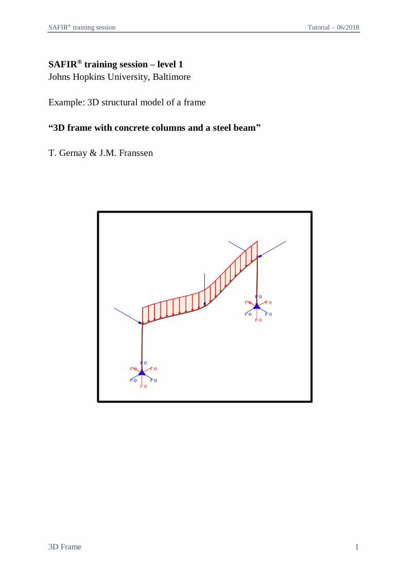
SAFIR® training session – level 1

Johns Hopkins University, Baltimore

Example: 3D structural model of a frame

“3D frame with concrete columns and a steel beam”

T. Gernay & J.M. Franssen


3D Frame 2

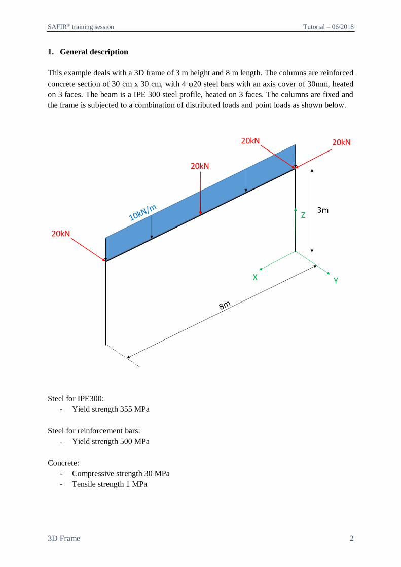
1. General description

This example deals with a 3D frame of 3 m height and 8 m length. The columns are reinforced

concrete section of 30 cm x 30 cm, with 4 φ20 steel bars with an axis cover of 30mm, heated

on 3 faces. The beam is a IPE 300 steel profile, heated on 3 faces. The columns are fixed and

the frame is subjected to a combination of distributed loads and point loads as shown below.

Steel for IPE300:

- Yield strength 355 MPa

Steel for reinforcement bars:

- Yield strength 500 MPa

Concrete:

- Compressive strength 30 MPa

- Tensile strength 1 MPa


3D Frame 3

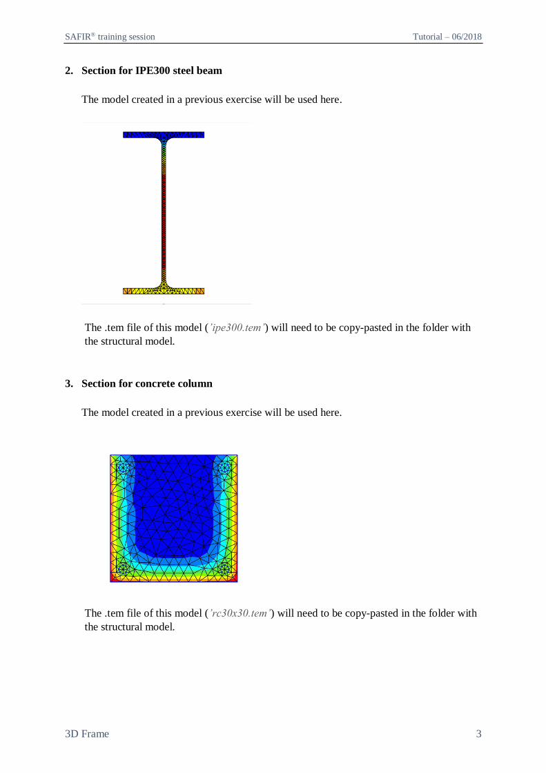
2. Section for IPE300 steel beam

The model created in a previous exercise will be used here.

The .tem file of this model (’ipe300.tem’) will need to be copy-pasted in the folder with

the structural model.

3. Section for concrete column

The model created in a previous exercise will be used here.

The .tem file of this model (’rc30x30.tem’) will need to be copy-pasted in the folder with

the structural model.


3D Frame 4

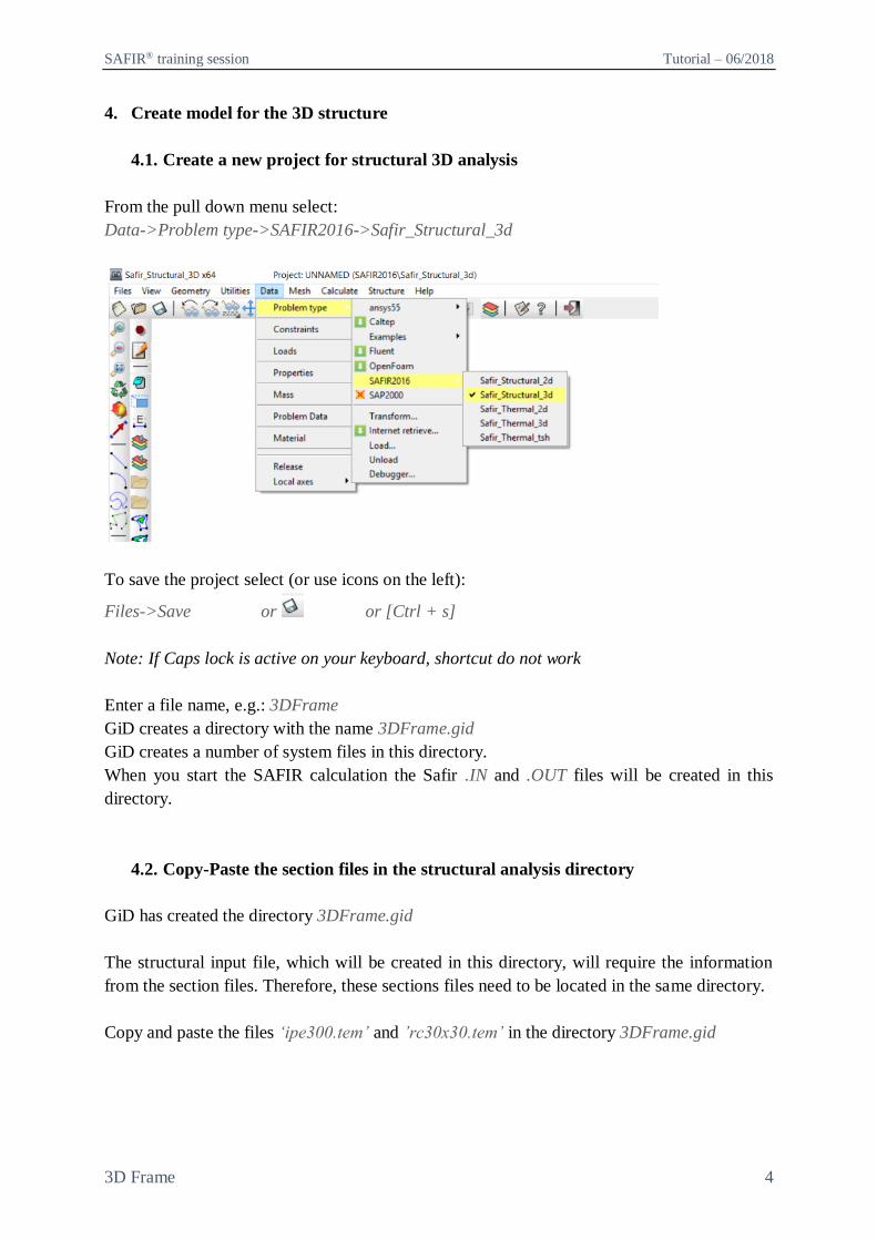
4. Create model for the 3D structure

4.1. Create a new project for structural 3D analysis

From the pull down menu select:

Data->Problem type->SAFIR2016->Safir_Structural_3d

To save the project select (or use icons on the left):

Files->Save or or [Ctrl + s]

Note: If Caps lock is active on your keyboard, shortcut do not work

Enter a file name, e.g.: 3DFrame

GiD creates a directory with the name 3DFrame.gid

GiD creates a number of system files in this directory.

When you start the SAFIR calculation the Safir .IN and .OUT files will be created in this

directory.

4.2. Copy-Paste the section files in the structural analysis directory

GiD has created the directory 3DFrame.gid

The structural input file, which will be created in this directory, will require the information

from the section files. Therefore, these sections files need to be located in the same directory.

Copy and paste the files ‘ipe300.tem’ and ’rc30x30.tem’ in the directory 3DFrame.gid


3D Frame 5

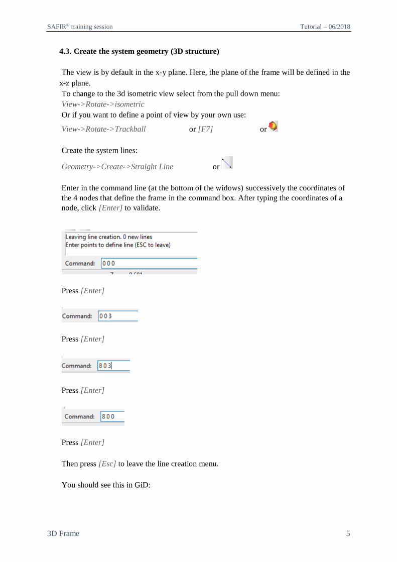
4.3. Create the system geometry (3D structure)

The view is by default in the x-y plane. Here, the plane of the frame will be defined in the

x-z plane.

To change to the 3d isometric view select from the pull down menu:

View->Rotate->isometric

Or if you want to define a point of view by your own use:

View->Rotate->Trackball or [F7] or

Create the system lines:

Geometry->Create->Straight Line or

Enter in the command line (at the bottom of the widows) successively the coordinates of

the 4 nodes that define the frame in the command box. After typing the coordinates of a

node, click [Enter] to validate.

Press [Enter]

Press [Enter]

Press [Enter]

Press [Enter]

Then press [Esc] to leave the line creation menu.

You should see this in GiD:


3D Frame 6

To see nodes and beams numbers select:

View->Label->All

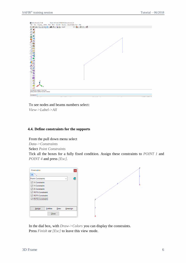
4.4. Define constraints for the supports

From the pull down menu select

Data->Constraints

Select Point Constraints

Tick all the boxes for a fully fixed condition. Assign these constraints to POINT 1 and

POINT 4 and press [Esc].

In the dial box, with Draw->Colors you can display the constraints.

Press Finish or [Esc] to leave this view mode.


3D Frame 7

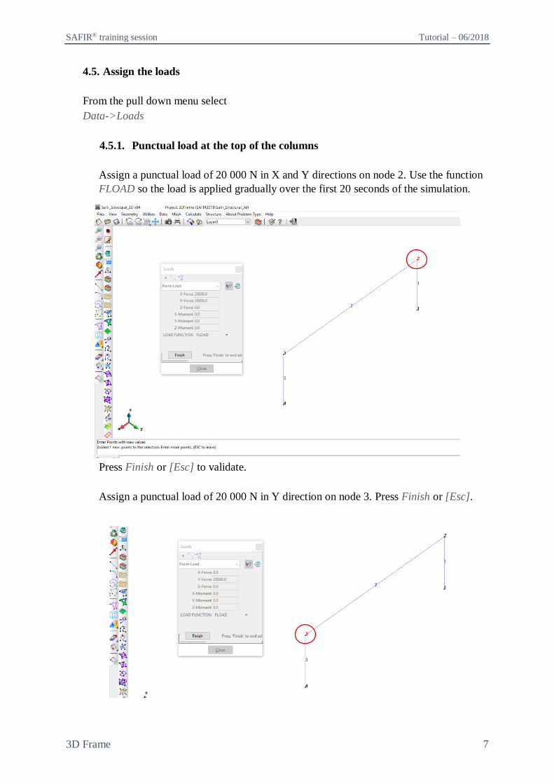
4.5. Assign the loads


Data->Loads

4.5.1. Punctual load at the top of the columns

Assign a punctual load of 20 000 N in X and Y directions on node 2. Use the function

FLOAD so the load is applied gradually over the first 20 seconds of the simulation.

Press Finish or [Esc] to validate.

Assign a punctual load of 20 000 N in Y direction on node 3. Press Finish or [Esc].


3D Frame 8

4.5.2. Distributed load on the beam

Assign a distributed load of -10 000 N/m in Z direction on the beam. Press Finish or

[Esc] to validate.

4.5.3. Punctual load at mid-span of the beam

First, create a node at mid-span of the beam.

Use Edit -> Divide -> Lines -> Num divisions: 2


3D Frame 9

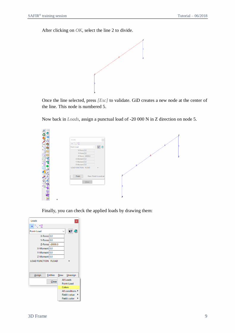
After clicking on OK, select the line 2 to divide.

Once the line selected, press [Esc] to validate. GiD creates a new node at the center of

the line. This node is numbered 5.

Now back in Loads, assign a punctual load of -20 000 N in Z direction on node 5.

Finally, you can check the applied loads by drawing them:


3D Frame 10

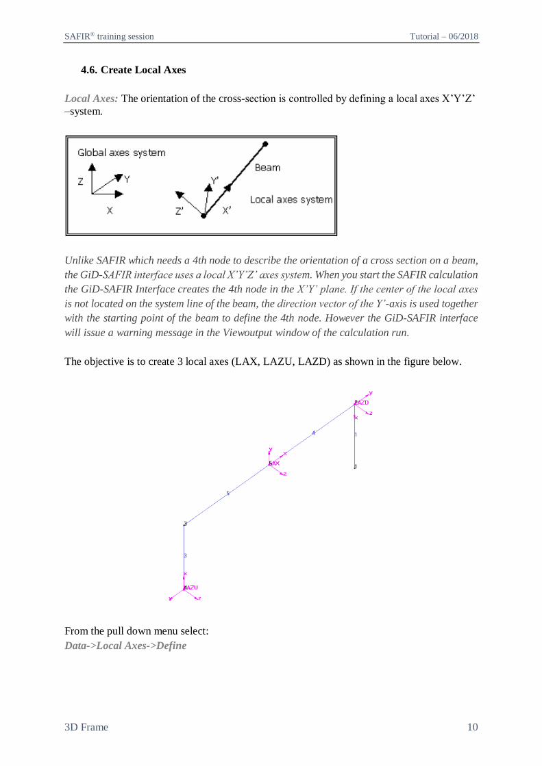
4.6. Create Local Axes

Local Axes: The orientation of the cross-section is controlled by defining a local axes X’Y’Z’

–system.

Unlike SAFIR which needs a 4th node to describe the orientation of a cross section on a beam,

the GiD-SAFIR interface uses a local X’Y’Z’ axes system. When you start the SAFIR calculation

the GiD-SAFIR Interface creates the 4th node in the X’Y’ plane. If the center of the local axes

is not located on the system line of the beam, the direction vector of the Y’-axis is used together

with the starting point of the beam to define the 4th node. However the GiD-SAFIR interface

will issue a warning message in the Viewoutput window of the calculation run.

The objective is to create 3 local axes (LAX, LAZU, LAZD) as shown in the figure below.


Data->Local Axes->Define


3D Frame 11

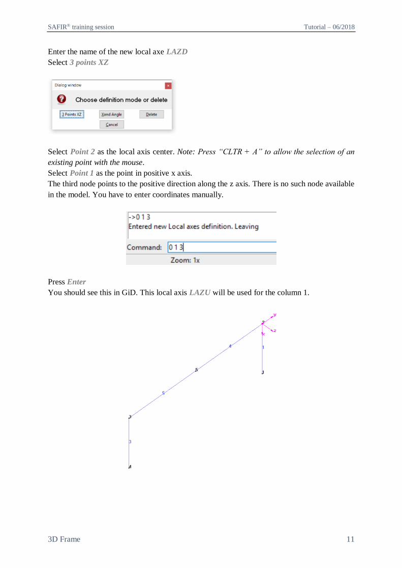
Enter the name of the new local axe LAZD

Select 3 points XZ

Select Point 2 as the local axis center. Note: Press “CLTR + A” to allow the selection of an

existing point with the mouse.

Select Point 1 as the point in positive x axis.

The third node points to the positive direction along the z axis. There is no such node available

in the model. You have to enter coordinates manually.

Press Enter

You should see this in GiD. This local axis LAZU will be used for the column 1.


3D Frame 12

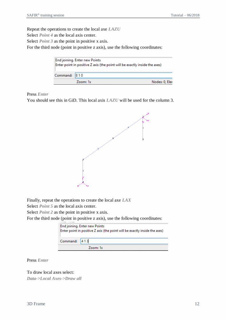
Repeat the operations to create the local axe LAZU

Select Point 4 as the local axis center.


For the third node (point in positive z axis), use the following coordinates:

Press Enter

You should see this in GiD. This local axis LAZU will be used for the column 3.

Finally, repeat the operations to create the local axe LAX

Select Point 5 as the local axis center.


For the third node (point in positive z axis), use the following coordinates:

Press Enter

To draw local axes select:

Data->Local Axes->Draw all


3D Frame 13

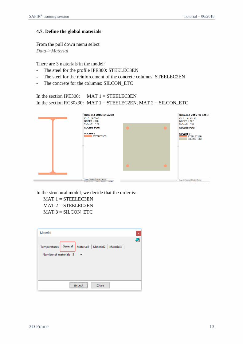
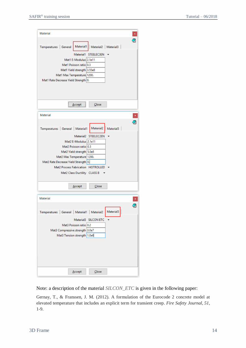
4.7. Define the global materials


Data->Material

There are 3 materials in the model:

- The steel for the profile IPE300: STEELEC3EN

- The steel for the reinforcement of the concrete columns: STEELEC2EN

- The concrete for the columns: SILCON_ETC

In the section IPE300: MAT 1 = STEELEC3EN

In the section RC30x30: MAT 1 = STEELEC2EN, MAT 2 = SILCON_ETC

In the structural model, we decide that the order is:

MAT 1 = STEELEC3EN

MAT 2 = STEELEC2EN

MAT 3 = SILCON_ETC


3D Frame 14

Note: a description of the material SILCON_ETC is given in the following paper:

Gernay, T., & Franssen, J. M. (2012). A formulation of the Eurocode 2 concrete model at

elevated temperature that includes an explicit term for transient creep. Fire Safety Journal, 51,

1-9.


3D Frame 15

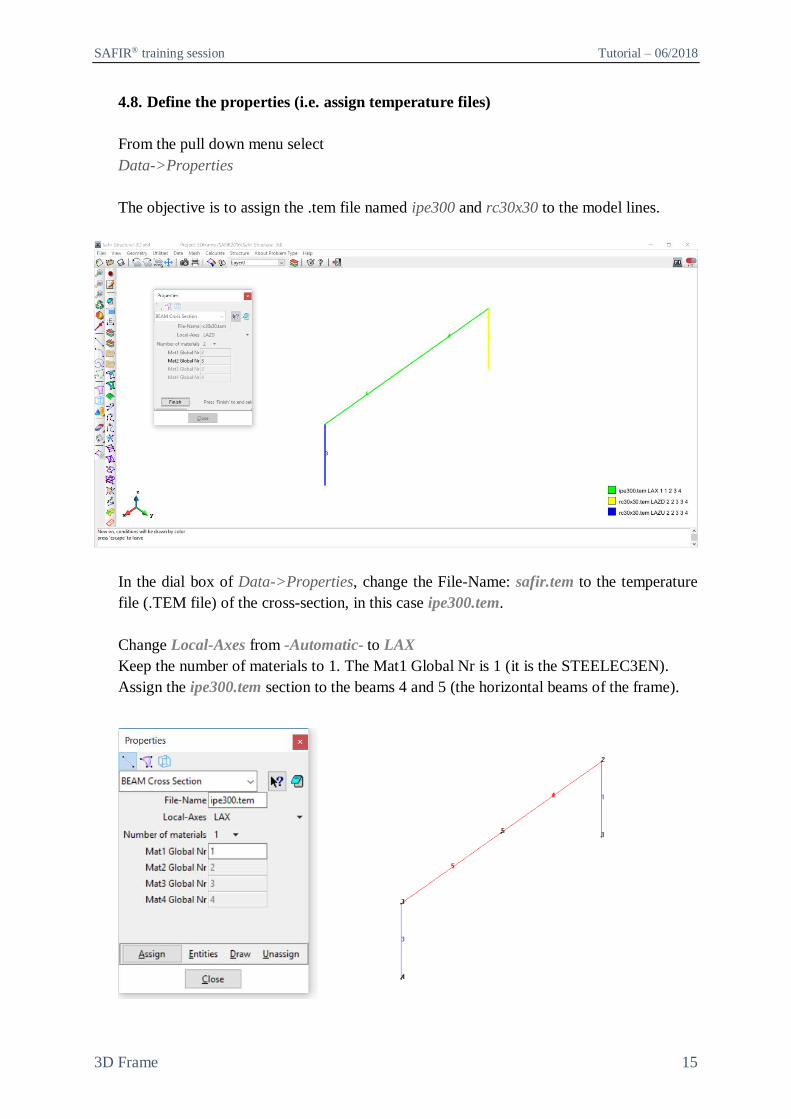
4.8. Define the properties (i.e. assign temperature files)


Data->Properties

The objective is to assign the .tem file named ipe300 and rc30x30 to the model lines.

In the dial box of Data->Properties, change the File-Name: safir.tem to the temperature

file (.TEM file) of the cross-section, in this case ipe300.tem.

Change Local-Axes from -Automatic- to LAX

Keep the number of materials to 1. The Mat1 Global Nr is 1 (it is the STEELEC3EN).

Assign the ipe300.tem section to the beams 4 and 5 (the horizontal beams of the frame).


3D Frame 16

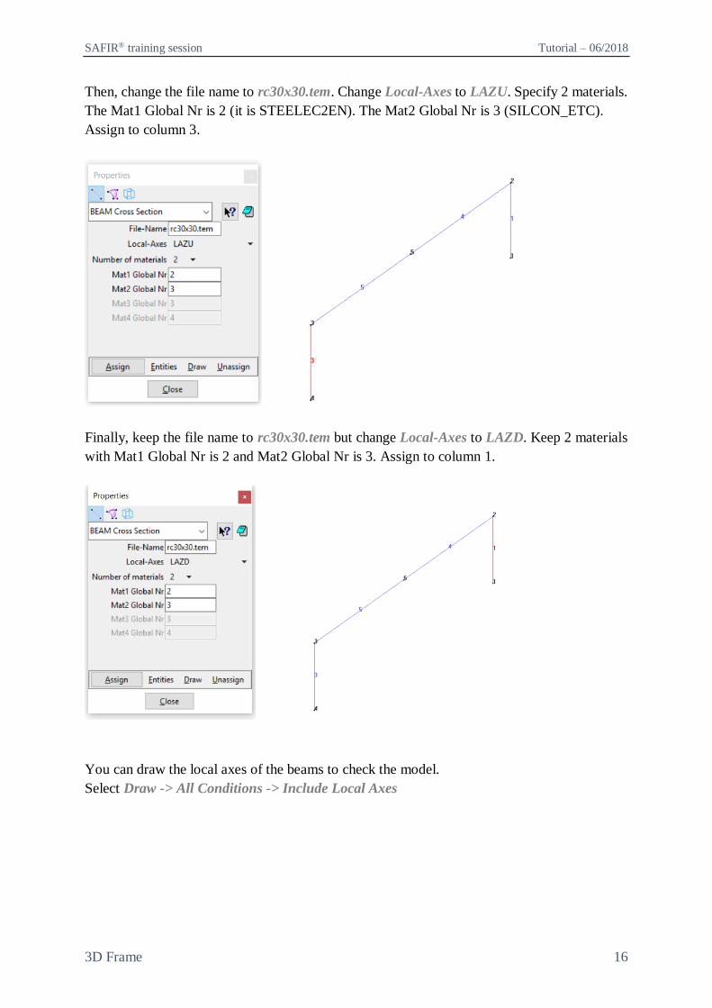
Then, change the file name to rc30x30.tem. Change Local-Axes to LAZU. Specify 2 materials.

The Mat1 Global Nr is 2 (it is STEELEC2EN). The Mat2 Global Nr is 3 (SILCON_ETC).

Assign to column 3.

Finally, keep the file name to rc30x30.tem but change Local-Axes to LAZD. Keep 2 materials

with Mat1 Global Nr is 2 and Mat2 Global Nr is 3. Assign to column 1.

You can draw the local axes of the beams to check the model.

Select Draw -> All Conditions -> Include Local Axes


3D Frame 17

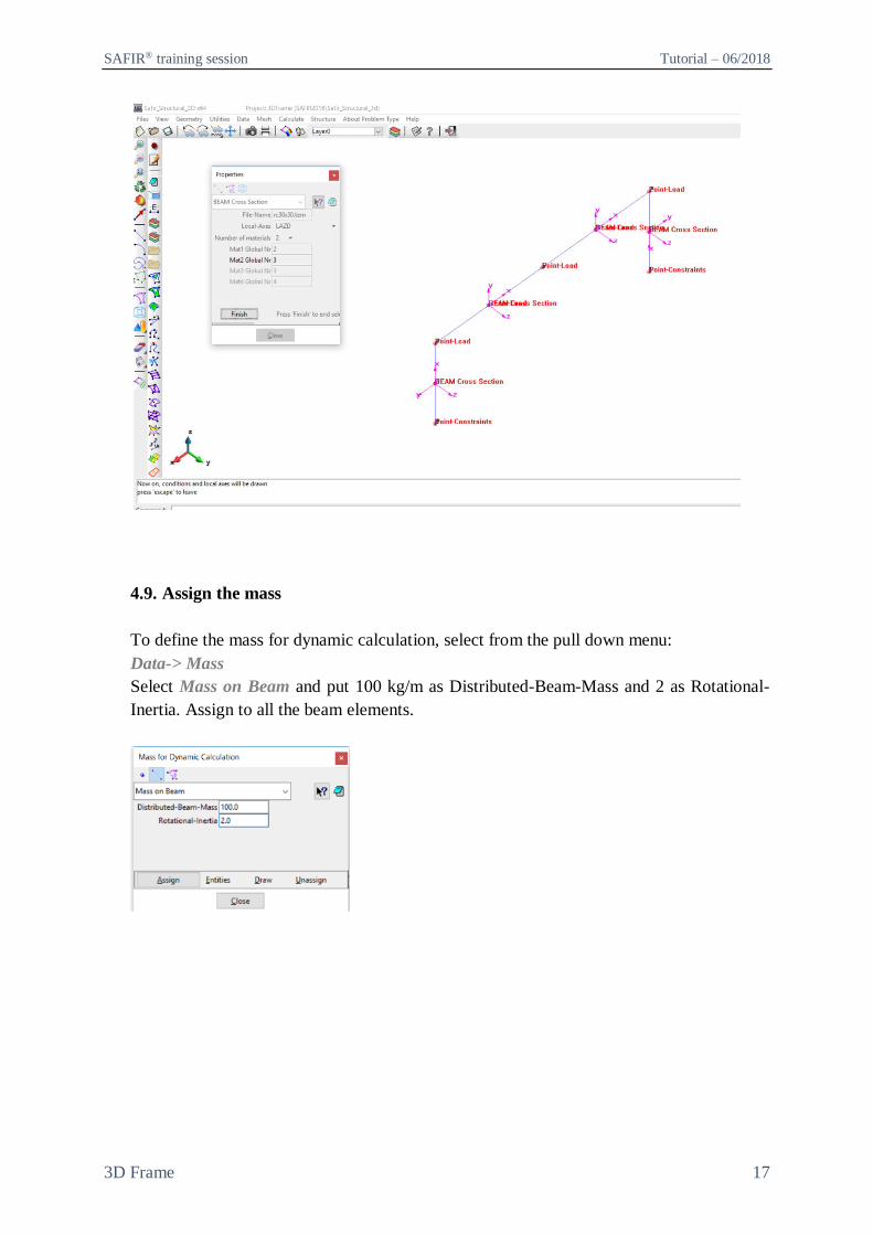
4.9. Assign the mass

To define the mass for dynamic calculation, select from the pull down menu:

Data-> Mass

Select Mass on Beam and put 100 kg/m as Distributed-Beam-Mass and 2 as Rotational-

Inertia. Assign to all the beam elements.


3D Frame 18

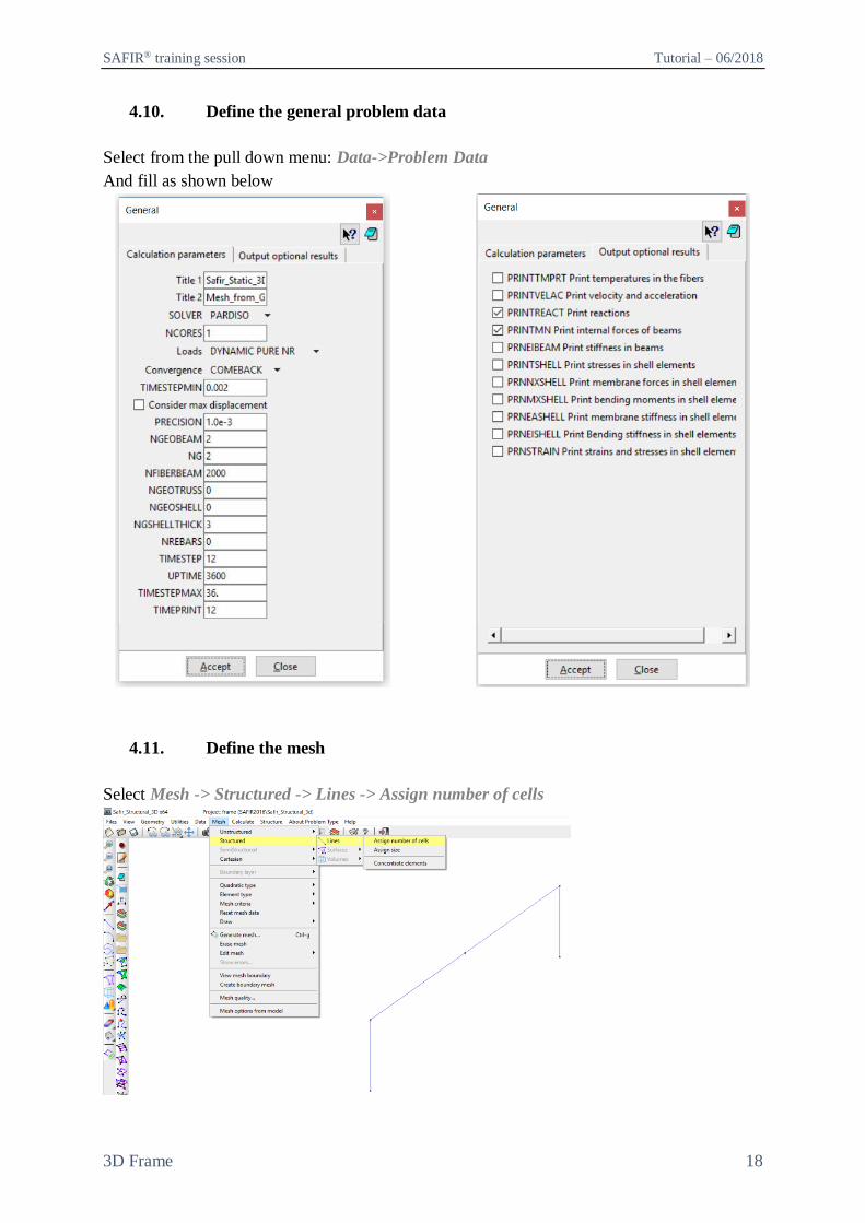
4.10. Define the general problem data

Select from the pull down menu: Data->Problem Data

And fill as shown below

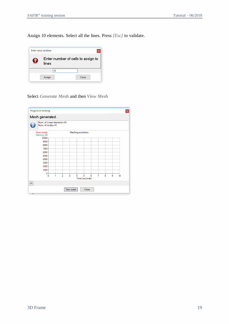
4.11. Define the mesh

Select Mesh -> Structured -> Lines -> Assign number of cells


3D Frame 19

Assign 10 elements. Select all the lines. Press [Esc] to validate.

Select Generate Mesh and then View Mesh


3D Frame 20

4.12. Start the calculation


Calculate->Calculate window

Click the Start button

You can follow the progress of the calculation by selecting Calculate->View process info

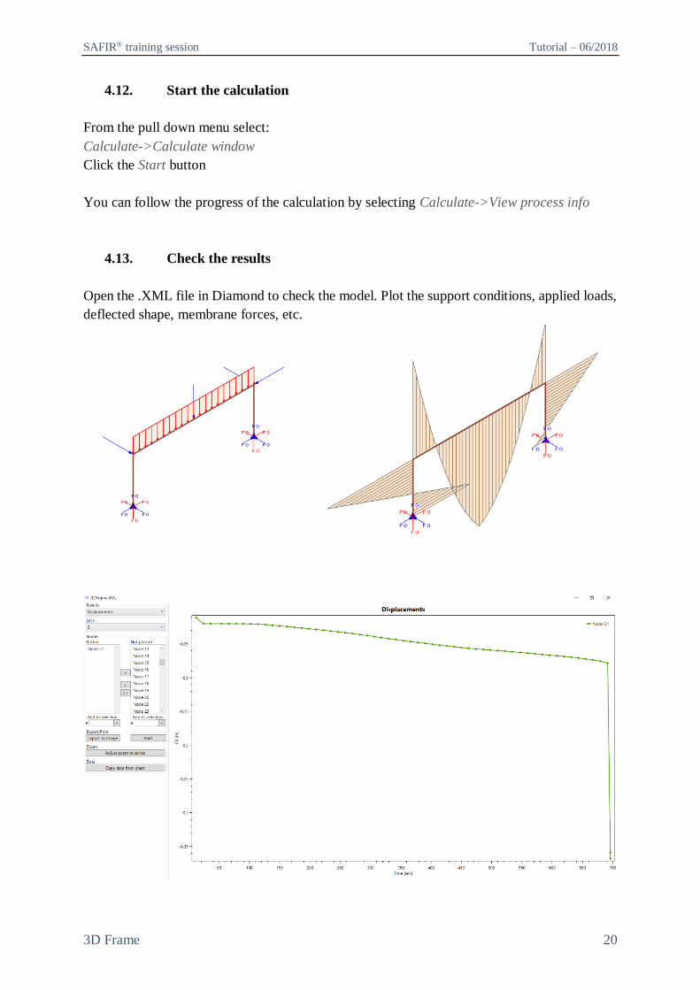
4.13. Check the results

Open the .XML file in Diamond to check the model. Plot the support conditions, applied loads,

deflected shape, membrane forces, etc.

Documents

3D frame with concrete columns and a steel beam