Embed Size (px)
Citation preview

7/28/2019 40cfr60AppA-2
http://slidepdf.com/reader/full/40cfr60appa-2 1/70
90
40 CFR Ch. I (7–1–09 Edition)Pt. 60, App. A–2
APPENDIX A–2 TO PART 60—TEST METHODS 2G THROUGH 3C
Method 2G—Determination of Stack Gas Ve-locity and Volumetric Flow Rate WithTwo-Dimensional Probes
Method 2H—Determination of Stack Gas Ve-locity Taking Into Account Velocity DecayNear the Stack Wall
Method 3—Gas analysis for the determina-tion of dry molecular weight
Method 3A—Determination of Oxygen andCarbon Dioxide Concentrations in Emis-sions From Stationary Sources (Instru-mental Analyzer Procedure)
Method 3B—Gas analysis for the determina-
tion of emission rate correction factor orexcess air
Method 3C—Determination of carbon diox-ide, methane, nitrogen, and oxygen fromstationary sourcesThe test methods in this appendix are re-
ferred to in § 60.8 (Performance Tests) and§ 60.11 (Compliance With Standards andMaintenance Requirements) of 40 CFR part60, subpart A (General Provisions). Specificuses of these test methods are described inthe standards of performance contained inthe subparts, beginning with Subpart D.
Within each standard of performance, asection title ‘‘Test Methods and Procedures’’is provided to: (1) Identify the test methodsto be used as reference methods to the facil-ity subject to the respective standard and (2)identify any special instructions or condi-
tions to be followed when applying a methodto the respective facility. Such instructions(for example, establish sampling rates, vol-umes, or temperatures) are to be used eitherin addition to, or as a substitute for proce-dures in a test method. Similarly, forsources subject to emission monitoring re-quirements, specific instructions pertainingto any use of a test method as a referencemethod are provided in the subpart or in Ap-pendix B.
Inclusion of methods in this appendix isnot intended as an endorsement or denial of their applicability to sources that are notsubject to standards of performance. Themethods are potentially applicable to othersources; however, applicability should beconfirmed by careful and appropriate evalua-tion of the conditions prevalent at such
sources.The approach followed in the formulationof the test methods involves specificationsfor equipment, procedures, and performance.In concept, a performance specification ap-proach would be preferable in all methodsbecause this allows the greatest flexibilityto the user. In practice, however, this ap-proach is impractical in most cases becauseperformance specifications cannot be estab-lished. Most of the methods described herein,therefore, involve specific equipment speci-fications and procedures, and only a few
methods in this appendix rely on perform-
ance criteria.
Minor changes in the test methods shouldnot necessarily affect the validity of the re-
sults and it is recognized that alternative
and equivalent methods exist. Section 60.8
provides authority for the Administrator tospecify or approve (1) equivalent methods, (2)
alternative methods, and (3) minor changes
in the methodology of the test methods. Itshould be clearly understood that unless oth-
erwise identified all such methods and
changes must have prior approval of the Ad-ministrator. An owner employing such meth-
ods or deviations from the test methods
without obtaining prior approval does so atthe risk of subsequent disapproval and re-
testing with approved methods.
Within the test methods, certain specific
equipment or procedures are recognized asbeing acceptable or potentially acceptable
and are specifically identified in the meth-
ods. The items identified as acceptable op-tions may be used without approval but
must be identified in the test report. The po-
tentially approvable options are cited as‘‘subject to the approval of the Adminis-
trator’’ or as ‘‘or equivalent.’’ Such poten-
tially approvable techniques or alternatives
may be used at the discretion of the ownerwithout prior approval. However, detailed
descriptions for applying these potentially
approvable techniques or alternatives arenot provided in the test methods. Also, the
potentially approvable options are not nec-essarily acceptable in all applications.Therefore, an owner electing to use such po-
tentially approvable techniques or alter-
natives is responsible for: (1) assuring thatthe techniques or alternatives are in fact ap-
plicable and are properly executed; (2) in-
cluding a written description of the alter-native method in the test report (the written
method must be clear and must be capable of
being performed without additional instruc-
tion, and the degree of detail should be simi-lar to the detail contained in the test meth-
ods); and (3) providing any rationale or sup-
porting data necessary to show the validityof the alternative in the particular applica-
tion. Failure to meet these requirements can
result in the Administrator’s disapproval of the alternative.
METHOD 2G—DETERMINATION OF STACK GAS
VELOCITY AND VOLUMETRIC FLOW RATE
WITH TWO-DIMENSIONAL PROBES
NOTE: This method does not include all of
the specifications (e.g., equipment and sup-
plies) and procedures (e.g., sampling) essen-tial to its performance. Some material has
been incorporated from other methods in
this part. Therefore, to obtain reliable re-sults, those using this method should have athorough knowledge of at least the following
VerDate Nov<24>2008 14:47 Aug 31, 2009 Jkt 217149 PO 00000 Frm 00100 Fmt 8010 Sfmt 8002 Y:\SGML\217149.XXX 217149

7/28/2019 40cfr60AppA-2
http://slidepdf.com/reader/full/40cfr60appa-2 2/70
91
Environmental Protection Agency Pt. 60, App. A–2, Meth. 2G
additional test methods: Methods 1, 2, 3 or
3A, and 4.
1.0 Scope and Application
1.1 This method is applicable for the de-
termination of yaw angle, near-axial veloc-
ity, and the volumetric flow rate of a gasstream in a stack or duct using a two-dimen-
sional (2–D) probe.
2.0 Summary of Method
2.1 A 2–D probe is used to measure the ve-
locity pressure and the yaw angle of the flow
velocity vector in a stack or duct. Alter-natively, these measurements may be made
by operating one of the three-dimensional (3–
D) probes described in Method 2F, in yaw de-termination mode only. From these meas-
urements and a determination of the stack
gas density, the average near-axial velocity
of the stack gas is calculated. The near-axialvelocity accounts for the yaw, but not the
pitch, component of flow. The average gas
volumetric flow rate in the stack or duct isthen determined from the average near-axial
velocity.
3.0 Definitions
3.1. Angle-measuring Device Rotational Off-
set (R ADO ). The rotational position of an
angle-measuring device relative to the ref-
erence scribe line, as determined during thepre-test rotational position check described
in section 8.3.3.2 Calibration Pitot Tube. The standard
(Prandtl type) pitot tube used as a reference
when calibrating a probe under this method.
3.3 Field Test. A set of measurements con-ducted at a specific unit or exhaust stack/duct to satisfy the applicable regulation(e.g., a three-run boiler performance test, asingle-or multiple-load nine-run relative ac-curacy test).
3.4 Full Scale of Pressure-measuring Device.
Full scale refers to the upper limit of themeasurement range displayed by the device.For bi-directional pressure gauges, full scaleincludes the entire pressure range from thelowest negative value to the highest positivevalue on the pressure scale.
3.5 Main probe. Refers to the probe headand that section of probe sheath directly at-
tached to the probe head. The main probesheath is distinguished from probe exten-sions, which are sections of sheath addedonto the main probe to extend its reach.
3.6 ‘‘May,’’ ‘‘Must,’’ ‘‘Shall,’’ ‘‘Should,’’ andthe imperative form of verbs.
3.6.1 ‘‘May’’ is used to indicate that a pro-vision of this method is optional.
3.6.2 ‘‘Must,’’ ‘‘Shall,’’ and the imperativeform of verbs (such as ‘‘record’’ or ‘‘enter’’)are used to indicate that a provision of thismethod is mandatory.
3.6.3 ‘‘Should’’ is used to indicate that aprovision of this method is not mandatory,but is highly recommended as good practice.
3.7 Method 1. Refers to 40 CFR part 60, ap-pendix A, ‘‘Method 1—Sample and velocitytraverses for stationary sources.’’
3.8 Method 2. Refers to 40 CFR part 60, ap-pendix A, ‘‘Method 2—Determination of stack gas velocity and volumetric flow rate(Type S pitot tube).’’
3.9 Method 2F. Refers to 40 CFR part 60, ap-pendix A, ‘‘Method 2F—Determination of stack gas velocity and volumetric flow ratewith three-dimensional probes.’’
3.10 Near-axial Velocity. The velocity vectorparallel to the axis of the stack or duct thataccounts for the yaw angle component of gasflow. The term ‘‘near-axial’’ is used herein toindicate that the velocity and volumetricflow rate results account for the measuredyaw angle component of flow at each meas-urement point.
3.11 Nominal Velocity. Refers to a wind tun-nel velocity setting that approximates theactual wind tunnel velocity to within ±1.5 m/sec (±5 ft/sec).
3.12 Pitch Angle. The angle between the axisof the stack or duct and the pitch componentof flow, i.e., the component of the total ve-locity vector in a plane defined by the tra-verse line and the axis of the stack or duct.(Figure 2G–1 illustrates the ‘‘pitch plane.’’)From the standpoint of a tester facing a testport in a vertical stack, the pitch componentof flow is the vector of flow moving from thecenter of the stack toward or away from thattest port. The pitch angle is the angle de-scribed by this pitch component of flow andthe vertical axis of the stack.
3.13 Readability. For the purposes of thismethod, readability for an analog measure-ment device is one half of the smallest scaledivision. For a digital measurement device,it is the number of decimals displayed by thedevice.
3.14 Reference Scribe Line. A line perma-nently inscribed on the main probe sheath(in accordance with section 6.1.5.1) to serveas a reference mark for determining yaw an-gles.
3.15 Reference Scribe Line Rotational Offset
(RSLO ). The rotational position of a probe’sreference scribe line relative to the probe’syaw-null position, as determined during theyaw angle calibration described in section10.5.
3.16 Response Time. The time required forthe measurement system to fully respond toa change from zero differential pressure andambient temperature to the stable stack orduct pressure and temperature readings at atraverse point.
3.17 Tested Probe. A probe that is beingcalibrated.
3.18 Three-dimensional (3–D) Probe. A direc-tional probe used to determine the velocity
VerDate Nov<24>2008 14:47 Aug 31, 2009 Jkt 217149 PO 00000 Frm 00101 Fmt 8010 Sfmt 8002 Y:\SGML\217149.XXX 217149

7/28/2019 40cfr60AppA-2
http://slidepdf.com/reader/full/40cfr60appa-2 3/70
92
40 CFR Ch. I (7–1–09 Edition)Pt. 60, App. A–2, Meth. 2G
pressure and the yaw and pitch angles in aflowing gas stream.
3.19 Two-dimensional (2–D) Probe. A direc-tional probe used to measure velocity pres-sure and yaw angle in a flowing gas stream.
3.20 Traverse Line. A diameter or axis ex-tending across a stack or duct on whichmeasurements of velocity pressure and flowangles are made.
3.21 Wind Tunnel Calibration Location. Apoint, line, area, or volume within the windtunnel test section at, along, or withinwhich probes are calibrated. At a particularwind tunnel velocity setting, the average ve-locity pressures at specified points at, along,or within the calibration location shall vary
by no more than 2 percent or 0.3 mm H20 (0.01in. H2O), whichever is less restrictive, fromthe average velocity pressure at the calibra-tion pitot tube location. Air flow at this lo-cation shall be axial, i.e., yaw and pitch an-gles within ±3° of 0°. Compliance with theseflow criteria shall be demonstrated by per-forming the procedures prescribed in sec-tions 10.1.1 and 10.1.2. For circular tunnels,no part of the calibration location may becloser to the tunnel wall than 10.2 cm (4 in.)or 25 percent of the tunnel diameter, which-ever is farther from the wall. For ellipticalor rectangular tunnels, no part of the cali-bration location may be closer to the tunnelwall than 10.2 cm (4 in.) or 25 percent of theapplicable cross-sectional axis, whichever isfarther from the wall.
3.22 Wind Tunnel with Documented Axial
Flow. A wind tunnel facility documented asmeeting the provisions of sections 10.1.1 (ve-locity pressure cross-check) and 10.1.2 (axialflow verification) using the procedures de-scribed in these sections or alternative pro-cedures determined to be technically equiva-lent.
3.23 Yaw Angle. The angle between theaxis of the stack or duct and the yaw compo-nent of flow, i.e., the component of the totalvelocity vector in a plane perpendicular tothe traverse line at a particular traversepoint. (Figure 2G–1 illustrates the ‘‘yawplane.’’) From the standpoint of a tester fac-ing a test port in a vertical stack, the yawcomponent of flow is the vector of flow mov-ing to the left or right from the center of thestack as viewed by the tester. (This is some-times referred to as ‘‘vortex flow,’’ i.e., flow
around the centerline of a stack or duct.)The yaw angle is the angle described by thisyaw component of flow and the vertical axisof the stack. The algebraic sign conventionis illustrated in Figure 2G–2.
3.24 Yaw Nulling. A procedure in which aType-S pitot tube or a 3–D probe is rotatedabout its axis in a stack or duct until a zerodifferential pressure reading (‘‘yaw null’’) isobtained. When a Type S probe is yaw-nulled, the rotational position of its impactport is 90° from the direction of flow in thestack or duct and the DP reading is zero.
When a 3–D probe is yaw-nulled, its impactpressure port (P1) faces directly into the di-rection of flow in the stack or duct and thedifferential pressure between pressure portsP2 and P3 is zero.
4.0 Interferences [Reserved]
5.0 Safety
5.1 This test method may involve haz-ardous operations and the use of hazardousmaterials or equipment. This method doesnot purport to address all of the safety prob-lems associated with its use. It is the respon-sibility of the user to establish and imple-ment appropriate safety and health practices
and to determine the applicability of regu-latory limitations before using this testmethod.
6.0 Equipment and Supplies
6.1 Two-dimensional Probes. Probes thatprovide both the velocity pressure and theyaw angle of the flow vector in a stack orduct, as listed in sections 6.1.1 and 6.1.2, qual-ify for use based on comprehensive wind tun-nel and field studies involving both inter-andintra-probe comparisons by multiple testteams. Each 2–D probe shall have a uniqueidentification number or code permanentlymarked on the main probe sheath. Eachprobe shall be calibrated prior to use accord-ing to the procedures in section 10. Manufac-turer-supplied calibration data shall be usedas example information only, except when
the manufacturer calibrates the probe asspecified in section 10 and provides completedocumentation.
6.1.1 Type S (Stausscheibe or reversetype) pitot tube. This is the same as speci-fied in Method 2, section 2.1, except for thefollowing additional specifications that en-able the pitot tube to accurately determinethe yaw component of flow. For the purposesof this method, the external diameter of thetubing used to construct the Type S pitottube (dimension Dt in Figure 2–2 of Method 2)shall be no less than 9.5 mm (3/8 in.). Thepitot tube shall also meet the followingalignment specifications. The angles a1, a2,b1, and b2, as shown in Method 2, Figure 2–3,shall not exceed ±2°. The dimensions w and z,shown in Method 2, Figure 2–3 shall not ex-ceed 0.5 mm (0.02 in.).
6.1.1.1 Manual Type S probe. This refersto a Type S probe that is positioned at indi-vidual traverse points and yaw nulled manu-ally by an operator.
6.1.1.2 Automated Type S probe. This re-fers to a system that uses a computer-con-trolled motorized mechanism to position theType S pitot head at individual traversepoints and perform yaw angle determina-tions.
6.1.2 Three-dimensional probes used in 2– D mode. A 3–D probe, as specified in sections6.1.1 through 6.1.3 of Method 2F, may, for the
VerDate Nov<24>2008 14:47 Aug 31, 2009 Jkt 217149 PO 00000 Frm 00102 Fmt 8010 Sfmt 8002 Y:\SGML\217149.XXX 217149

7/28/2019 40cfr60AppA-2
http://slidepdf.com/reader/full/40cfr60appa-2 4/70
93
Environmental Protection Agency Pt. 60, App. A–2, Meth. 2G
purposes of this method, be used in a two-di-mensional mode (i.e., measuring yaw angle,but not pitch angle). When the 3–D probe isused as a 2–D probe, only the velocity pres-sure and yaw-null pressure are obtainedusing the pressure taps referred to as P1, P2,and P3. The differential pressure P1 –P2 is afunction of total velocity and corresponds tothe DP obtained using the Type S probe. Thedifferential pressure P2 –P3 is used to yawnull the probe and determine the yaw angle.The differential pressure P4 –P5, which is afunction of pitch angle, is not measuredwhen the 3–D probe is used in 2–D mode.
6.1.3 Other probes. [Reserved]6.1.4 Probe sheath. The probe shaft shall
include an outer sheath to: (1) provide a sur-face for inscribing a permanent referencescribe line, (2) accommodate attachment of an angle-measuring device to the probeshaft, and (3) facilitate precise rotationalmovement of the probe for determining yawangles. The sheath shall be rigidly attachedto the probe assembly and shall enclose allpressure lines from the probe head to the far-thest position away from the probe headwhere an angle-measuring device may be at-tached during use in the field. The sheath of the fully assembled probe shall be suffi-ciently rigid and straight at all rotationalpositions such that, when one end of theprobe shaft is held in a horizontal position,the fully extended probe meets the hori-zontal straightness specifications indicatedin section 8.2 below.
6.1.5 Scribe lines.6.1.5.1 Reference scribe line. A permanent
line, no greater than 1.6 mm (1/16 in.) inwidth, shall be inscribed on each manualprobe that will be used to determine yaw an-gles of flow. This line shall be placed on themain probe sheath in accordance with theprocedures described in section 10.4 and isused as a reference position for installationof the yaw angle-measuring device on theprobe. At the discretion of the tester, thescribe line may be a single line segmentplaced at a particular position on the probesheath (e.g., near the probe head), multipleline segments placed at various locationsalong the length of the probe sheath (e.g., atevery position where a yaw angle-measuringdevice may be mounted), or a single contin-uous line extending along the full length of
the probe sheath.6.1.5.2 Scribe line on probe extensions. Apermanent line may also be inscribed on anyprobe extension that will be attached to themain probe in performing field testing. Thisallows a yaw angle-measuring device mount-ed on the extension to be readily alignedwith the reference scribe line on the mainprobe sheath.
6.1.5.3 Alignment specifications. Thisspecification shall be met separately, usingthe procedures in section 10.4.1, on the mainprobe and on each probe extension. The rota-
tional position of the scribe line or scribe
line segments on the main probe or any
probe extension must not vary by more than
2°. That is, the difference between the min-
imum and maximum of all of the rotational
angles that are measured along the fulllength of the main probe or the probe exten-
sion must not exceed 2°.6.1.6 Probe and system characteristics to
ensure horizontal stability.
6.1.6.1 For manual probes, it is rec-
ommended that the effective length of the
probe (coupled with a probe extension, if nec-essary) be at least 0.9 m (3 ft.) longer than
the farthest traverse point mark on the
probe shaft away from the probe head. Theoperator should maintain the probe’s hori-zontal stability when it is fully inserted into
the stack or duct. If a shorter probe is used,
the probe should be inserted through a bush-ing sleeve, similar to the one shown in Fig-
ure 2G–3, that is installed on the test port;
such a bushing shall fit snugly around theprobe and be secured to the stack or duct
entry port in such a manner as to maintain
the probe’s horizontal stability when fullyinserted into the stack or duct.
6.1.6.2 An automated system that includes
an external probe casing with a transport
system shall have a mechanism for main-taining horizontal stability comparable to
that obtained by manual probes following
the provisions of this method. The auto-mated probe assembly shall also be con-
structed to maintain the alignment and posi-tion of the pressure ports during sampling ateach traverse point. The design of the probe
casing and transport system shall allow the
probe to be removed from the stack or duct
and checked through direct physical meas-urement for angular position and insertion
depth.
6.1.7 The tubing that is used to connectthe probe and the pressure-measuring device
should have an inside diameter of at least 3.2
mm (1 ⁄ 8 in.), to reduce the time required for
pressure equilibration, and should be asshort as practicable.
6.1.8 If a detachable probe head without a
sheath [e.g., a pitot tube, typically 15.2 to30.5 cm (6 to 12 in.) in length] is coupled with
a probe sheath and calibrated in a wind tun-
nel in accordance with the yaw angle cali-
bration procedure in section 10.5, the probehead shall remain attached to the probe
sheath during field testing in the same con-
figuration and orientation as calibrated.Once the detachable probe head is uncoupled
or re-oriented, the yaw angle calibration of
the probe is no longer valid and must be re-peated before using the probe in subsequent
field tests.
6.2 Yaw Angle-measuring Device. One of
the following devices shall be used for meas-urement of the yaw angle of flow.
VerDate Nov<24>2008 14:47 Aug 31, 2009 Jkt 217149 PO 00000 Frm 00103 Fmt 8010 Sfmt 8002 Y:\SGML\217149.XXX 217149

7/28/2019 40cfr60AppA-2
http://slidepdf.com/reader/full/40cfr60appa-2 5/70
94
40 CFR Ch. I (7–1–09 Edition)Pt. 60, App. A–2, Meth. 2G
6.2.1 Digital inclinometer. This refers to adigital device capable of measuring and dis-playing the rotational position of the probeto within ±1°. The device shall be able to belocked into position on the probe sheath orprobe extension, so that it indicates theprobe’s rotational position throughout thetest. A rotational position collar block thatcan be attached to the probe sheath (similarto the collar shown in Figure 2G–4) may berequired to lock the digital inclinometerinto position on the probe sheath.
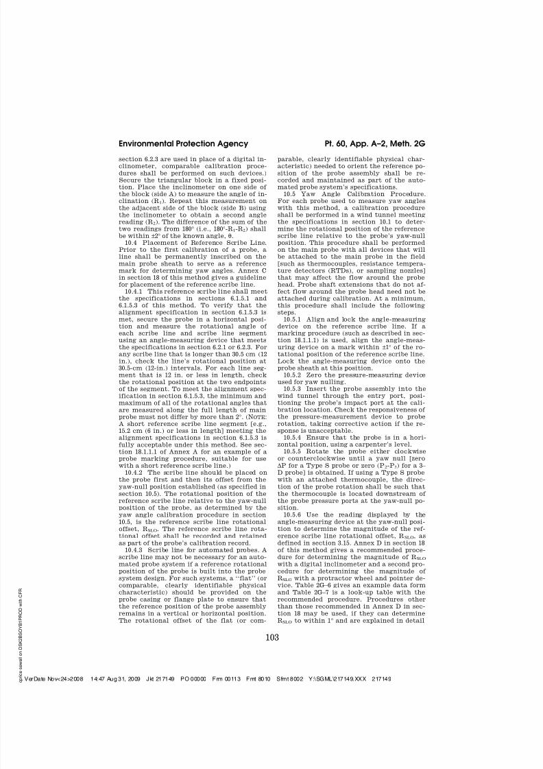
6.2.2 Protractor wheel and pointer assem-bly. This apparatus, similar to that shown inFigure 2G–5, consists of the following compo-nents.
6.2.2.1 A protractor wheel that can be at-tached to a port opening and set in a fixedrotational position to indicate the yaw angleposition of the probe’s scribe line relative tothe longitudinal axis of the stack or duct.The protractor wheel must have a measure-ment ring on its face that is no less than 17.8cm (7 in.) in diameter, shall be able to be ro-tated to any angle and then locked into posi-tion on the stack or duct test port, and shallindicate angles to a resolution of 1°.
6.2.2.2 A pointer assembly that includesan indicator needle mounted on a collar thatcan slide over the probe sheath and be lockedinto a fixed rotational position on the probesheath. The pointer needle shall be of suffi-cient length, rigidity, and sharpness to allowthe tester to determine the probe’s angularposition to within 1° from the markings on
the protractor wheel. Corresponding to theposition of the pointer, the collar must havea scribe line to be used in aligning the point-er with the scribe line on the probe sheath.
6.2.3 Other yaw angle-measuring devices.Other angle-measuring devices with a manu-facturer’s specified precision of 1° or bettermay be used, if approved by the Adminis-trator.
6.3 Probe Supports and Stabilization De-vices. When probes are used for determiningflow angles, the probe head should be kept ina stable horizontal position. For probeslonger than 3.0 m (10 ft.), the section of theprobe that extends outside the test port shallbe secured. Three alternative devices aresuggested for maintaining the horizontal po-sition and stability of the probe shaft duringflow angle determinations and velocity pres-sure measurements: (1) monorails installedabove each port, (2) probe stands on whichthe probe shaft may be rested, or (3) bushingsleeves of sufficient length secured to thetest ports to maintain probes in a horizontalposition. Comparable provisions shall bemade to ensure that automated systemsmaintain the horizontal position of the probein the stack or duct. The physical character-istics of each test platform may dictate themost suitable type of stabilization device.Thus, the choice of a specific stabilizationdevice is left to the judgement of the testers.
6.4 Differential Pressure Gauges. The ve-locity pressure (DP) measuring devices usedduring wind tunnel calibrations and fieldtesting shall be either electronicmanometers (e.g., pressure transducers),fluid manometers, or mechanical pressuregauges (e.g., MagnehelicD gauges). Use of electronic manometers is recommended.Under low velocity conditions, use of elec-tronic manometers may be necessary to ob-tain acceptable measurements.
6.4.1 Differential pressure-measuring de-vice. This refers to a device capable of meas-uring pressure differentials and having areadability of ±1 percent of full scale. The de-vice shall be capable of accurately meas-
uring the maximum expected pressure dif-ferential. Such devices are used to determinethe following pressure measurements: veloc-ity pressure, static pressure, and yaw-nullpressure. For an inclined-vertical manom-eter, the readability specification of ±1 per-cent shall be met separately using the re-spective full-scale upper limits of the in-clined anvertical portions of the scales. Tothe extent practicable, the device shall be se-lected such that most of the pressure read-ings are between 10 and 90 percent of the de-vice’s full-scale measurement range (as de-fined in section 3.4). In addition, pressure-measuring devices should be selected suchthat the zero does not drift by more than 5percent of the average expected pressurereadings to be encountered during the fieldtest. This is particularly important under
low pressure conditions.6.4.2 Gauge used for yaw nulling. The dif-
ferential pressure-measuring device chosenfor yaw nulling the probe during the windtunnel calibrations and field testing shall bebi-directional, i.e., capable of reading bothpositive and negative differential pressures.If a mechanical, bi-directional pressuregauge is chosen, it shall have a full-scalerange no greater than 2.6 cm (i.e., ¥1.3 to+1.3 cm) [1 in. H2O (i.e., ¥0.5 in. to +0.5 in.)].
6.4.3 Devices for calibrating differentialpressure-measuring devices. A precision ma-nometer (e.g., a U-tube, inclined, or inclined-vertical manometer, or micromanometer) orNIST (National Institute of Standards andTechnology) traceable pressure source shallbe used for calibrating differential pressure-measuring devices. The device shall be main-tained under laboratory conditions or in asimilar protected environment (e.g., a cli-mate-controlled trailer). It shall not be usedin field tests. The precision manometer shallhave a scale gradation of 0.3 mm H2O (0.01 in.H2O), or less, in the range of 0 to 5.1 cm H 2O(0 to 2 in. H2O) and 2.5 mm H2O (0.1 in. H2O),or less, in the range of 5.1 to 25.4 cm H2O (2to 10 in. H2O). The manometer shall havemanufacturer’s documentation that it meetsan accuracy specification of at least 0.5 per-cent of full scale. The NIST-traceable pres-sure source shall be recertified annually.
VerDate Nov<24>2008 14:47 Aug 31, 2009 Jkt 217149 PO 00000 Frm 00104 Fmt 8010 Sfmt 8002 Y:\SGML\217149.XXX 217149

7/28/2019 40cfr60AppA-2
http://slidepdf.com/reader/full/40cfr60appa-2 6/70
95
Environmental Protection Agency Pt. 60, App. A–2, Meth. 2G
6.4.4 Devices used for post-test calibrationcheck. A precision manometer meeting thespecifications in section 6.4.3, a pressure-measuring device or pressure source with adocumented calibration traceable to NIST,or an equivalent device approved by the Ad-ministrator shall be used for the post-testcalibration check. The pressure-measuringdevice shall have a readability equivalent toor greater than the tested device. The pres-sure source shall be capable of generatingpressures between 50 and 90 percent of therange of the tested device and known towithin ±1 percent of the full scale of the test-ed device. The pressure source shall be recer-tified annually.
6.5 Data Display and Capture Devices.Electronic manometers (if used) shall be cou-pled with a data display device (such as adigital panel meter, personal computer dis-play, or strip chart) that allows the tester toobserve and validate the pressure measure-ments taken during testing. They shall alsobe connected to a data recorder (such as adata logger or a personal computer with datacapture software) that has the ability tocompute and retain the appropriate averagevalue at each traverse point, identified bycollection time and traverse point.
6.6 Temperature Gauges. For field tests, athermocouple or resistance temperature de-tector (RTD) capable of measuring tempera-ture to within ±3°C (±5°F) of the stack orduct temperature shall be used. The thermo-couple shall be attached to the probe such
that the sensor tip does not touch any metal.The position of the thermocouple relative tothe pressure port face openings shall be inthe same configuration as used for the probecalibrations in the wind tunnel. Temperaturegauges used for wind tunnel calibrationsshall be capable of measuring temperature towithin ±0.6°C (±1°F) of the temperature of theflowing gas stream in the wind tunnel.
6.7 Stack or Duct Static Pressure Meas-urement. The pressure-measuring deviceused with the probe shall be as specified insection 6.4 of this method. The static tap of a standard (Prandtl type) pitot tube or oneleg of a Type S pitot tube with the face open-ing planes positioned parallel to the gas flowmay be used for this measurement. Also ac-ceptable is the pressure differential readingof P1-Pbar from a five-hole prism-shaped 3–D
probe, as specified in section 6.1.1 of Method2F (such as the Type DA or DAT probe), withthe P1 pressure port face opening positionedparallel to the gas flow in the same manneras the Type S probe. However, the 3–D spher-ical probe, as specified in section 6.1.2 of Method 2F, is unable to provide this meas-urement and shall not be used to take staticpressure measurements. Static pressuremeasurement is further described in section8.11.
6.8 Barometer. Same as Method 2, section2.5.
6.9 Gas Density Determination Equip-ment. Method 3 or 3A shall be used to deter-mine the dry molecular weight of the stackor duct gas. Method 4 shall be used for mois-ture content determination and computationof stack or duct gas wet molecular weight.Other methods may be used, if approved bythe Administrator.
6.10 Calibration Pitot Tube. Same asMethod 2, section 2.7.
6.11 Wind Tunnel for Probe Calibration.Wind tunnels used to calibrate velocityprobes must meet the following design speci-fications.
6.11.1 Test section cross-sectional area.The flowing gas stream shall be confined
within a circular, rectangular, or ellipticalduct. The cross-sectional area of the tunnelmust be large enough to ensure fully devel-oped flow in the presence of both the calibra-tion pitot tube and the tested probe. Thecalibration site, or ‘‘test section,’’ of thewind tunnel shall have a minimum diameterof 30.5 cm (12 in.) for circular or ellipticalduct cross-sections or a minimum width of 30.5 cm (12 in.) on the shorter side for rectan-gular cross-sections. Wind tunnels shall meetthe probe blockage provisions of this sectionand the qualification requirements pre-scribed in section 10.1. The projected area of the portion of the probe head, shaft, and at-tached devices inside the wind tunnel duringcalibration shall represent no more than 4percent of the cross-sectional area of thetunnel. The projected area shall include the
combined area of the calibration pitot tubeand the tested probe if both probes areplaced simultaneously in the same cross-sec-tional plane in the wind tunnel, or the largerprojected area of the two probes if they areplaced alternately in the wind tunnel.
6.11.2 Velocity range and stability. Thewind tunnel should be capable of maintain-ing velocities between 6.1 m/sec and 30.5 m/sec (20 ft/sec and 100 ft/sec). The wind tunnelshall produce fully developed flow patternsthat are stable and parallel to the axis of theduct in the test section.
6.11.3 Flow profile at the calibration loca-tion. The wind tunnel shall provide axialflow within the test section calibration loca-tion (as defined in section 3.21). Yaw andpitch angles in the calibration location shallbe within ±3° of 0°. The procedure for deter-
mining that this requirement has been metis described in section 10.1.2.6.11.4 Entry ports in the wind tunnel test
section.6.11.4.1 Port for tested probe. A port shall
be constructed for the tested probe. Thisport shall be located to allow the head of thetested probe to be positioned within the windtunnel calibration location (as defined insection 3.21). The tested probe shall be ableto be locked into the 0° pitch angle position.To facilitate alignment of the probe duringcalibration, the test section should include a
VerDate Nov<24>2008 14:47 Aug 31, 2009 Jkt 217149 PO 00000 Frm 00105 Fmt 8010 Sfmt 8002 Y:\SGML\217149.XXX 217149

7/28/2019 40cfr60AppA-2
http://slidepdf.com/reader/full/40cfr60appa-2 7/70
96
40 CFR Ch. I (7–1–09 Edition)Pt. 60, App. A–2, Meth. 2G
window constructed of a transparent mate-rial to allow the tested probe to be viewed.
6.11.4.2 Port for verification of axial flow.Depending on the equipment selected to con-duct the axial flow verification prescribed insection 10.1.2, a second port, located 90° fromthe entry port for the tested probe, may beneeded to allow verification that the gasflow is parallel to the central axis of the testsection. This port should be located and con-structed so as to allow one of the probes de-scribed in section 10.1.2.2 to access the sametest point(s) that are accessible from theport described in section 6.11.4.1.
6.11.4.3 Port for calibration pitot tube.The calibration pitot tube shall be used inthe port for the tested probe or in a separateentry port. In either case, all measurementswith the calibration pitot tube shall be madeat the same point within the wind tunnelover the course of a probe calibration. Themeasurement point for the calibration pitottube shall meet the same specifications fordistance from the wall and for axial flow asdescribed in section 3.21 for the wind tunnelcalibration location.
7.0 Reagents and Standards [Reserved]
8.0 Sample Collection and Analysis
8.1 Equipment Inspection and Set Up
8.1.1 All 2–D and 3–D probes, differentialpressure-measuring devices, yaw angle-meas-uring devices, thermocouples, and barom-eters shall have a current, valid calibrationbefore being used in a field test. (See sec-tions 10.3.3, 10.3.4, and 10.5 through 10.10 forthe applicable calibration requirements.)
8.1.2 Before each field use of a Type Sprobe, perform a visual inspection to verifythe physical condition of the pitot tube.Record the results of the inspection. If theface openings are noticeably misaligned orthere is visible damage to the face openings,the probe shall not be used until repaired,the dimensional specifications verified (ac-cording to the procedures in section 10.2.1),and the probe recalibrated.
8.1.3 Before each field use of a 3–D probe,perform a visual inspection to verify thephysical condition of the probe head accord-ing to the procedures in section 10.2 of Meth-od 2F. Record the inspection results on aform similar to Table 2F–1 presented inMethod 2F. If there is visible damage to the3–D probe, the probe shall not be used untilit is recalibrated.
8.1.4 After verifying that the physicalcondition of the probe head is acceptable, setup the apparatus using lengths of flexibletubing that are as short as practicable.Surge tanks installed between the probe andpressure-measuring device may be used todampen pressure fluctuations provided thatan adequate measurement system responsetime (see section 8.8) is maintained.
8.2 Horizontal Straightness Check. A hor-izontal straightness check shall be per-formed before the start of each field test, ex-cept as otherwise specified in this section.Secure the fully assembled probe (includingthe probe head and all probe shaft exten-sions) in a horizontal position using a sta-tionary support at a point along the probeshaft approximating the location of thestack or duct entry port when the probe issampling at the farthest traverse point fromthe stack or duct wall. The probe shall be ro-tated to detect bends. Use an angle-meas-uring device or trigonometry to determinethe bend or sag between the probe head andthe secured end. (See Figure 2G–6.) Probes
that are bent or sag by more than 5° shallnot be used. Although this check does notapply when the probe is used for a verticaltraverse, care should be taken to avoid theuse of bent probes when conducting verticaltraverses. If the probe is constructed of arigid steel material and consists of a mainprobe without probe extensions, this checkneed only be performed before the initialfield use of the probe, when the probe is re-calibrated, when a change is made to the de-sign or material of the probe assembly, andwhen the probe becomes bent. With suchprobes, a visual inspection shall be made of the fully assembled probe before each fieldtest to determine if a bend is visible. Theprobe shall be rotated to detect bends. Theinspection results shall be documented in thefield test report. If a bend in the probe is
visible, the horizontal straightness checkshall be performed before the probe is used.
8.3 Rotational Position Check. Beforeeach field test, and each time an extension isadded to the probe during a field test, a rota-tional position check shall be performed onall manually operated probes (except asnoted in section 8.3.5 below) to ensure that,throughout testing, the angle-measuring de-vice is either: aligned to within ±1° of the ro-tational position of the reference scribe line;or is affixed to the probe such that the rota-tional offset of the device from the referencescribe line is known to within ±1°. This checkshall consist of direct measurements of therotational positions of the reference scribeline and angle-measuring device sufficient toverify that these specifications are met.Annex A in section 18 of this method gives
recommended procedures for performing therotational position check, and Table 2G–2gives an example data form. Proceduresother than those recommended in Annex Ain section 18 may be used, provided theydemonstrate whether the alignment speci-fication is met and are explained in detail inthe field test report.
8.3.1 Angle-measuring device rotationaloffset. The tester shall maintain a record of the angle-measuring device rotational offset,RADO, as defined in section 3.1. Note thatRADO is assigned a value of 0° when the angle-
VerDate Nov<24>2008 14:47 Aug 31, 2009 Jkt 217149 PO 00000 Frm 00106 Fmt 8010 Sfmt 8002 Y:\SGML\217149.XXX 217149

7/28/2019 40cfr60AppA-2
http://slidepdf.com/reader/full/40cfr60appa-2 8/70
97
Environmental Protection Agency Pt. 60, App. A–2, Meth. 2G
measuring device is aligned to within ±1° of the rotational position of the referencescribe line. The RADO shall be used to deter-mine the yaw angle of flow in accordancewith section 8.9.4.
8.3.2 Sign of angle-measuring device rota-tional offset. The sign of RADO is positivewhen the angle-measuring device (as viewedfrom the ‘‘tail’’ end of the probe) is posi-tioned in a clockwise direction from the ref-erence scribe line and negative when the de-vice is positioned in a counterclockwise di-rection from the reference scribe line.
8.3.3 Angle-measuring devices that can beindependently adjusted (e.g., by means of aset screw), after being locked into position
on the probe sheath, may be used. However,the RADO must also take into account thisadjustment.
8.3.4 Post-test check. If probe extensionsremain attached to the main probe through-out the field test, the rotational positioncheck shall be repeated, at a minimum, atthe completion of the field test to ensurethat the angle-measuring device has re-mained within ±2° of its rotational positionestablished prior to testing. At the discre-tion of the tester, additional checks may beconducted after completion of testing at anysample port or after any test run. If the ±2°specification is not met, all measurementsmade since the last successful rotational po-sition check must be repeated. Section18.1.1.3 of Annex A provides an example pro-cedure for performing the post-test check.
8.3.5 Exceptions.8.3.5.1 A rotational position check neednot be performed if, for measurements takenat all velocity traverse points, the yawangle-measuring device is mounted andaligned directly on the reference scribe linespecified in sections 6.1.5.1 and 6.1.5.3 and noindependent adjustments, as described insection 8.3.3, are made to device’s rotationalposition.
8.3.5.2 If extensions are detached and re-attached to the probe during a field test, arotational position check need only be per-formed the first time an extension is addedto the probe, rather than each time the ex-tension is re-attached, if the probe extensionis designed to be locked into a mechanicallyfixed rotational position (e.g., through theuse of interlocking grooves), that can re-es-
tablish the initial rotational position towithin ±1°.8.4 Leak Checks. A pre-test leak check
shall be conducted before each field test. Apost-test check shall be performed at the endof the field test, but additional leak checksmay be conducted after any test run orgroup of test runs. The post-test check mayalso serve as the pre-test check for the nextgroup of test runs. If any leak check isfailed, all runs since the last passed leakcheck are invalid. While performing the leakcheck procedures, also check each pressure
device’s responsiveness to changes in pres-sure.
8.4.1 To perform the leak check on a TypeS pitot tube, pressurize the pitot impactopening until at least 7.6 cm H2O (3 in. H2O)velocity pressure, or a pressure cor-responding to approximately 75 percent of the pressure device’s measurement scale,whichever is less, registers on the pressuredevice; then, close off the impact opening.The pressure shall remain stable (±2.5 mmH2O, ±0.10 in. H2O) for at least 15 seconds. Re-peat this procedure for the static pressureside, except use suction to obtain the re-quired pressure. Other leak-check proceduresmay be used, if approved by the Adminis-
trator.8.4.2 To perform the leak check on a 3–D
probe, pressurize the probe’s impact (P1)opening until at least 7.6 cm H2O (3 in. H2O)velocity pressure, or a pressure cor-responding to approximately 75 percent of the pressure device’s measurement scale,whichever is less, registers on the pressuredevice; then, close off the impact opening.The pressure shall remain stable (±2.5 mmH2O, ±0.10 in. H2O) for at least 15 seconds.Check the P2 and P3 pressure ports in thesame fashion. Other leak-check proceduresmay be used, if approved by the Adminis-trator.
8.5 Zeroing the Differential Pressure-measuring Device. Zero each differentialpressure-measuring device, including the de-vice used for yaw nulling, before each field
test. At a minimum, check the zero aftereach field test. A zero check may also be per-formed after any test run or group of testruns. For fluid manometers and mechanicalpressure gauges (e.g., MagnehelicD gauges),the zero reading shall not deviate from zeroby more than ±0.8 mm H2O (±0.03 in. H2O) orone minor scale division, whichever is great-er, between checks. For electronicmanometers, the zero reading shall not devi-ate from zero between checks by more than:±0.3 mm H2O (±0.01 in. H2O), for full scalesless than or equal to 5.1 cm H2O (2.0 in. H2O);or ±0.8 mm H2O (±0.03 in. H2O), for full scalesgreater than 5.1 cm H2O (2.0 in. H2O). (NOTE:If negative zero drift is not directly readable,estimate the reading based on the position of the gauge oil in the manometer or of theneedle on the pressure gauge.) In addition,
for all pressure-measuring devices exceptthose used exclusively for yaw nulling, thezero reading shall not deviate from zero bymore than 5 percent of the average measureddifferential pressure at any distinct processcondition or load level. If any zero check isfailed at a specific process condition or loadlevel, all runs conducted at that process con-dition or load level since the last passed zerocheck are invalid.
8.6 Traverse Point Verification. The num-ber and location of the traverse points shallbe selected based on Method 1 guidelines.
VerDate Nov<24>2008 14:47 Aug 31, 2009 Jkt 217149 PO 00000 Frm 00107 Fmt 8010 Sfmt 8002 Y:\SGML\217149.XXX 217149

7/28/2019 40cfr60AppA-2
http://slidepdf.com/reader/full/40cfr60appa-2 9/70
98
40 CFR Ch. I (7–1–09 Edition)Pt. 60, App. A–2, Meth. 2G
The stack or duct diameter and port nipplelengths, including any extension of the portnipples into the stack or duct, shall beverified the first time the test is performed;retain and use this information for subse-quent field tests, updating it as required.Physically measure the stack or duct dimen-sions or use a calibrated laser device; do notuse engineering drawings of the stack orduct. The probe length necessary to reacheach traverse point shall be recorded towithin ±6.4 mm (±1 ⁄ 4 in.) and, for manualprobes, marked on the probe sheath. In de-termining these lengths, the tester shalltake into account both the distance that theport flange projects outside of the stack and
the depth that any port nipple extends intothe gas stream. The resulting point positionsshall reflect the true distances from the in-side wall of the stack or duct, so that whenthe tester aligns any of the markings withthe outside face of the stack port, theprobe’s impact port shall be located at theappropriate distance from the inside wall forthe respective Method 1 traverse point. Be-fore beginning testing at a particular loca-tion, an out-of-stack or duct verificationshall be performed on each probe that will beused to ensure that these position markingsare correct. The distances measured duringthe verification must agree with the pre-viously calculated distances to within ±1 ⁄ 4 in.For manual probes, the traverse point posi-tions shall be verified by measuring the dis-tance of each mark from the probe’s impact
pressure port (the P1 port for a 3-D probe). Acomparable out-of-stack test shall be per-formed on automated probe systems. Theprobe shall be extended to each of the pre-scribed traverse point positions. Then, theaccuracy of the positioning for each traversepoint shall be verified by measuring the dis-tance between the port flange and theprobe’s impact pressure port.
8.7 Probe Installation. Insert the probeinto the test port. A solid material shall beused to seal the port.
8.8 System Response Time. Determine theresponse time of the probe measurement sys-tem. Insert and position the ‘‘cold’’ probe (atambient temperature and pressure) at anyMethod 1 traverse point. Read and record theprobe differential pressure, temperature, andelapsed time at 15-second intervals until sta-
ble readings for both pressure and tempera-ture are achieved. The response time is thelonger of these two elapsed times. Record theresponse time.
8.9 Sampling.8.9.1 Yaw angle measurement protocol.
With manual probes, yaw angle measure-ments may be obtained in two alternativeways during the field test, either by using ayaw angle-measuring device (e.g., digital in-clinometer) affixed to the probe, or using aprotractor wheel and pointer assembly. Forhorizontal traversing, either approach may
be used. For vertical traversing, i.e., whenmeasuring from on top or into the bottom of a horizontal duct, only the protractor wheeland pointer assembly may be used. Withautomated probes, curve-fitting protocolsmay be used to obtain yaw-angle measure-ments.
8.9.1.1 If a yaw angle-measuring device af-fixed to the probe is to be used, lock the de-vice on the probe sheath, aligning it eitheron the reference scribe line or in the rota-tional offset position established under sec-tion 8.3.1.
8.9.1.2 If a protractor wheel and pointerassembly is to be used, follow the proceduresin Annex B of this method.
8.9.1.3 Curve-fitting procedures. Curve-fit-ting routines sweep through a range of yawangles to create curves correlating pressureto yaw position. To find the zero yaw posi-tion and the yaw angle of flow, the curvefound in the stack is computationally com-pared to a similar curve that was previouslygenerated under controlled conditions in awind tunnel. A probe system that uses acurve-fitting routine for determining theyaw-null position of the probe head may beused, provided that it is verified in a windtunnel to be able to determine the yaw angleof flow to within ±1°.
8.9.1.4 Other yaw angle determinationprocedures. If approved by the Adminis-trator, other procedures for determining yawangle may be used, provided that they areverified in a wind tunnel to be able to per-
form the yaw angle calibration procedure asdescribed in section 10.5.
8.9.2 Sampling strategy. At each traversepoint, first yaw-null the probe, as describedin section 8.9.3, below. Then, with the probeoriented into the direction of flow, measureand record the yaw angle, the differentialpressure and the temperature at the traversepoint, after stable readings are achieved, inaccordance with sections 8.9.4 and 8.9.5. Atthe start of testing in each port (i.e., after aprobe has been inserted into the flue gasstream), allow at least the response time toelapse before beginning to take measure-ments at the first traverse point accessedfrom that port. Provided that the probe isnot removed from the flue gas stream, meas-urements may be taken at subsequent tra-verse points accessed from the same test
port without waiting again for the responsetime to elapse.8.9.3 Yaw-nulling procedure. In prepara-
tion for yaw angle determination, the probemust first be yaw nulled. After positioningthe probe at the appropriate traverse point,perform the following procedures.
8.9.3.1 For Type S probes, rotate the probeuntil a null differential pressure reading isobtained. The direction of the probe rotationshall be such that the thermocouple is lo-cated downstream of the probe pressureports at the yaw-null position. Rotate the
VerDate Nov<24>2008 14:47 Aug 31, 2009 Jkt 217149 PO 00000 Frm 00108 Fmt 8010 Sfmt 8002 Y:\SGML\217149.XXX 217149

7/28/2019 40cfr60AppA-2
http://slidepdf.com/reader/full/40cfr60appa-2 10/70
99
Environmental Protection Agency Pt. 60, App. A–2, Meth. 2G
probe 90° back from the yaw-null position toorient the impact pressure port into the di-rection of flow. Read and record the angledisplayed by the angle-measuring device.
8.9.3.2 For 3-D probes, rotate the probeuntil a null differential pressure reading (thedifference in pressures across the P2 and P3
pressure ports is zero, i.e., P2=P3) is indi-cated by the yaw angle pressure gauge. Readand record the angle displayed by the angle-measuring device.
8.9.3.3 Sign of the measured angle. Theangle displayed on the angle-measuring de-vice is considered positive when the probe’simpact pressure port (as viewed from the‘‘tail’’ end of the probe) is oriented in aclockwise rotational position relative to thestack or duct axis and is considered negativewhen the probe’s impact pressure port is ori-ented in a counterclockwise rotational posi-tion (see Figure 2G–7).
8.9.4 Yaw angle determination. After per-forming the applicable yaw-nulling proce-dure in section 8.9.3, determine the yawangle of flow according to one of the fol-lowing procedures. Special care must be ob-served to take into account the signs of therecorded angle reading and all offsets.
8.9.4.1 Direct-reading. If all rotational off-sets are zero or if the angle-measuring devicerotational offset (RADO) determined in sec-tion 8.3 exactly compensates for the scribeline rotational offset (RSLO) determined insection 10.5, then the magnitude of the yawangle is equal to the displayed angle-meas-
uring device reading from section 8.9.3.1 or8.9.3.2. The algebraic sign of the yaw angle isdetermined in accordance with section8.9.3.3. [NOTE: Under certain circumstances(e.g., testing of horizontal ducts) a 90° ad-justment to the angle-measuring devicereadings may be necessary to obtain the cor-rect yaw angles.]
8.9.4.2 Compensation for rotational offsetsduring data reduction. When the angle-meas-uring device rotational offset does not com-pensate for reference scribe line rotationaloffset, the following procedure shall be usedto determine the yaw angle:
(a) Enter the reading indicated by theangle-measuring device from section 8.9.3.1or 8.9.3.2.
(b) Associate the proper algebraic signfrom section 8.9.3.3 with the reading in step
(a).(c) Subtract the reference scribe line rota-
tional offset, RSLO, from the reading in step(b).
(d) Subtract the angle-measuring devicerotational offset, RADO, if any, from the re-sult obtained in step (c).
(e) The final result obtained in step (d) isthe yaw angle of flow.
[NOTE: It may be necessary to first apply a90° adjustment to the reading in step (a), inorder to obtain the correct yaw angle.]
8.9.4.3 Record the yaw angle measure-
ments on a form similar to Table 2G–3.
8.9.5 Impact velocity determination.
Maintain the probe rotational position es-
tablished during the yaw angle determina-
tion. Then, begin recording the pressure-
measuring device readings. These pressure
measurements shall be taken over a sam-
pling period of sufficiently long duration to
ensure representative readings at each tra-
verse point. If the pressure measurements
are determined from visual readings of the
pressure device or display, allow sufficienttime to observe the pulsation in the readings
to obtain a sight-weighted average, which is
then recorded manually. If an automateddata acquisition system (e.g., data logger,
computer-based data recorder, strip chart re-
corder) is used to record the pressure meas-urements, obtain an integrated average of all
pressure readings at the traverse point.
Stack or duct gas temperature measure-
ments shall be recorded, at a minimum, onceat each traverse point. Record all necessary
data as shown in the example field data form
(Table 2G–3).
8.9.6 Alignment check. For manually op-
erated probes, after the required yaw angle
and differential pressure and temperature
measurements have been made at each tra-verse point, verify (e.g., by visual inspection)
that the yaw angle-measuring device has re-
mained in proper alignment with the ref-erence scribe line or with the rotational off-
set position established in section 8.3. If, fora particular traverse point, the angle-meas-uring device is found to be in proper align-
ment, proceed to the next traverse point;
otherwise, re-align the device and repeat theangle and differential pressure measure-
ments at the traverse point. In the course of
a traverse, if a mark used to properly align
the angle-measuring device (e.g., as de-scribed in section 18.1.1.1) cannot be located,
re-establish the alignment mark before pro-
ceeding with the traverse.
8.10 Probe Plugging. Periodically check
for plugging of the pressure ports by observ-
ing the responses on the pressure differentialreadouts. Plugging causes erratic results or
sluggish responses. Rotate the probe to de-
termine whether the readouts respond in the
expected direction. If plugging is detected,
correct the problem and repeat the affectedmeasurements.
8.11 Static Pressure. Measure the staticpressure in the stack or duct using the
equipment described in section 6.7.
8.11.1 If a Type S probe is used for this
measurement, position the probe at or be-tween any traverse point(s) and rotate the
probe until a null differential pressure read-
ing is obtained. Disconnect the tubing fromone of the pressure ports; read and record the
DP. For pressure devices with one-directional
VerDate Nov<24>2008 14:47 Aug 31, 2009 Jkt 217149 PO 00000 Frm 00109 Fmt 8010 Sfmt 8002 Y:\SGML\217149.XXX 217149

7/28/2019 40cfr60AppA-2
http://slidepdf.com/reader/full/40cfr60appa-2 11/70
100
40 CFR Ch. I (7–1–09 Edition)Pt. 60, App. A–2, Meth. 2G
scales, if a deflection in the positive direc-
tion is noted with the negative side discon-
nected, then the static pressure is positive.
Likewise, if a deflection in the positive di-
rection is noted with the positive side dis-
connected, then the static pressure is nega-
tive.
8.11.2 If a 3–D probe is used for this meas-
urement, position the probe at or between
any traverse point(s) and rotate the probe
until a null differential pressure reading is
obtained at P2 –P3. Rotate the probe 90°. Dis-
connect the P2 pressure side of the probe and
read the pressure P1 –Pbar and record as the
static pressure. (NOTE: The spherical probe,
specified in section 6.1.2 of Method 2F, is un-able to provide this measurement and shall
not be used to take static pressure measure-
ments.)
8.12 Atmospheric Pressure. Determine the
atmospheric pressure at the sampling ele-
vation during each test run following the
procedure described in section 2.5 of Method
2.
8.13 Molecular Weight. Determine the
stack or duct gas dry molecular weight. For
combustion processes or processes that emit
essentially CO2, O2, CO, and N2, use Method 3
or 3A. For processes emitting essentially air,
an analysis need not be conducted; use a dry
molecular weight of 29.0. Other methods may
be used, if approved by the Administrator.
8.14 Moisture. Determine the moisture
content of the stack gas using Method 4 orequivalent.
8.15 Data Recording and Calculations.
Record all required data on a form similar to
Table 2G–3.
8.15.1 2–D probe calibration coefficient.
When a Type S pitot tube is used in the field,
the appropriate calibration coefficient as de-
termined in section 10.6 shall be used to per-
form velocity calculations. For calibrated
Type S pitot tubes, the A-side coefficient
shall be used when the A-side of the tube
faces the flow, and the B-side coefficient
shall be used when the B-side faces the flow.
8.15.2 3–D calibration coefficient. When a
3–D probe is used to collect data with this
method, follow the provisions for the calibra-
tion of 3–D probes in section 10.6 of Method
2F to obtain the appropriate velocity cali-
bration coefficient (F2 as derived using Equa-tion 2F–2 in Method 2F) corresponding to a
pitch angle position of 0°.8.15.3 Calculations. Calculate the yaw-ad-
justed velocity at each traverse point using
the equations presented in section 12.2. Cal-
culate the test run average stack gas veloc-
ity by finding the arithmetic average of the
point velocity results in accordance with
sections 12.3 and 12.4, and calculate the stack
gas volumetric flow rate in accordance with
section 12.5 or 12.6, as applicable.
9.0 Quality Control
9.1 Quality Control Activities. In conjunc-tion with the yaw angle determination andthe pressure and temperature measurementsspecified in section 8.9, the following qualitycontrol checks should be performed.
9.1.1 Range of the differential pressuregauge. In accordance with the specificationsin section 6.4, ensure that the proper dif-ferential pressure gauge is being used for therange of DP values encountered. If it is nec-essary to change to a more sensitive gauge,replace the gauge with a gauge calibrated ac-cording to section 10.3.3, perform the leakcheck described in section 8.4 and the zero
check described in section 8.5, and repeat thedifferential pressure and temperature read-ings at each traverse point.
9.1.2 Horizontal stability check. For hori-zontal traverses of a stack or duct, visuallycheck that the probe shaft is maintained ina horizontal position prior to taking a pres-sure reading. Periodically, during a test run,the probe’s horizontal stability should beverified by placing a carpenter’s level, a dig-ital inclinometer, or other angle-measuringdevice on the portion of the probe sheaththat extends outside of the test port. A com-parable check should be performed by auto-mated systems.
10.0 Calibration
10.1 Wind Tunnel Qualification Checks.To qualify for use in calibrating probes, a
wind tunnel shall have the design featuresspecified in section 6.11 and satisfy the fol-lowing qualification criteria. The velocitypressure cross-check in section 10.1.1 andaxial flow verification in section 10.1.2 shallbe performed before the initial use of thewind tunnel and repeated immediately afterany alteration occurs in the wind tunnel’sconfiguration, fans, interior surfaces,straightening vanes, controls, or other prop-erties that could reasonably be expected toalter the flow pattern or velocity stability inthe tunnel. The owner or operator of a windtunnel used to calibrate probes according tothis method shall maintain records docu-menting that the wind tunnel meets the re-quirements of sections 10.1.1 and 10.1.2 andshall provide these records to the Adminis-trator upon request.
10.1.1 Velocity pressure cross-check. Toverify that the wind tunnel produces thesame velocity at the tested probe head as atthe calibration pitot tube impact port, per-form the following cross-check. Take threedifferential pressure measurements at thefixed calibration pitot tube location, usingthe calibration pitot tube specified in sec-tion 6.10, and take three measurements withthe calibration pitot tube at the wind tunnelcalibration location, as defined in section3.21. Alternate the measurements betweenthe two positions. Perform this procedure at
VerDate Nov<24>2008 14:47 Aug 31, 2009 Jkt 217149 PO 00000 Frm 00110 Fmt 8010 Sfmt 8002 Y:\SGML\217149.XXX 217149

7/28/2019 40cfr60AppA-2
http://slidepdf.com/reader/full/40cfr60appa-2 12/70
101
Environmental Protection Agency Pt. 60, App. A–2, Meth. 2G
the lowest and highest velocity settings atwhich the probes will be calibrated. Recordthe values on a form similar to Table 2G–4.At each velocity setting, the average veloc-ity pressure obtained at the wind tunnelcalibration location shall be within ±2 per-cent or 2.5 mm H2O (0.01 in. H2O), whicheveris less restrictive, of the average velocitypressure obtained at the fixed calibrationpitot tube location. This comparative checkshall be performed at 2.5-cm (1-in.), or small-er, intervals across the full length, width,and depth (if applicable) of the wind tunnelcalibration location. If the criteria are notmet at every tested point, the wind tunnelcalibration location must be redefined, so
that acceptable results are obtained at everypoint. Include the results of the velocitypressure cross-check in the calibration datasection of the field test report. (See section16.1.4.)
10.1.2 Axial flow verification. The fol-lowing procedures shall be performed todemonstrate that there is fully developedaxial flow within the wind tunnel calibrationlocation and at the calibration pitot tube lo-cation. Two options are available to conductthis check.
10.1.2.1 Using a calibrated 3–D probe. Aprobe that has been previously calibrated ina wind tunnel with documented axial flow(as defined in section 3.22) may be used toconduct this check. Insert the calibrated 3–Dprobe into the wind tunnel test section usingthe tested probe port. Following the proce-
dures in sections 8.9 and 12.2 of Method 2F,determine the yaw and pitch angles at allthe point(s) in the test section where the ve-locity pressure cross-check, as specified insection 10.1.1, is performed. This includes allthe points in the calibration location and thepoint where the calibration pitot tube will belocated. Determine the yaw and pitch anglesat each point. Repeat these measurements atthe highest and lowest velocities at whichthe probes will be calibrated. Record the val-ues on a form similar to Table 2G–5. Eachmeasured yaw and pitch angle shall be with-in ±3° of 0°. Exceeding the limits indicatesunacceptable flow in the test section. Untilthe problem is corrected and acceptable flowis verified by repetition of this procedure,the wind tunnel shall not be used for calibra-tion of probes. Include the results of the
axial flow verification in the calibrationdata section of the field test report. (See sec-tion 16.1.4.)
10.1.2.2 Using alternative probes. Axialflow verification may be performed using anuncalibrated prism-shaped 3–D probe (e.g.,DA or DAT probe) or an uncalibrated wedgeprobe. (Figure 2G–8 illustrates a typicalwedge probe.) This approach requires use of two ports: the tested probe port and a secondport located 90° from the tested probe port.Each port shall provide access to all thepoints within the wind tunnel test section
where the velocity pressure cross-check, as
specified in section 10.1.1, is conducted. The
probe setup shall include establishing a ref-erence yaw-null position on the probe sheath
to serve as the location for installing the
angle-measuring device. Physical design fea-tures of the DA, DAT, and wedge probes arerelied on to determine the reference posi-tion. For the DA or DAT probe, this ref-erence position can be determined by settinga digital inclinometer on the flat facet wherethe P1 pressure port is located and then iden-tifying the rotational position on the probesheath where a second angle-measuring de-vice would give the same angle reading. Thereference position on a wedge probe shaft canbe determined either geometrically or byplacing a digital inclinometer on each side of the wedge and rotating the probe untilequivalent readings are obtained. With thelatter approach, the reference position is therotational position on the probe sheathwhere an angle-measuring device would givea reading of 0°. After installation of theangle-measuring device in the reference yaw-null position on the probe sheath, determinethe yaw angle from the tested port. Repeatthis measurement using the 90° offset port,which provides the pitch angle of flow. De-termine the yaw and pitch angles at all thepoint(s) in the test section where the veloc-ity pressure cross-check, as specified in sec-tion 10.1.1, is performed. This includes all thepoints in the wind tunnel calibration loca-tion and the point where the calibration
pitot tube will be located. Perform thischeck at the highest and lowest velocities atwhich the probes will be calibrated. Recordthe values on a form similar to Table 2G–5.Each measured yaw and pitch angle shall bewithin ±3° of 0°. Exceeding the limits indi-cates unacceptable flow in the test section.Until the problem is corrected and accept-able flow is verified by repetition of this pro-cedure, the wind tunnel shall not be used forcalibration of probes. Include the results inthe probe calibration report.
10.1.3 Wind tunnel audits.
10.1.3.1 Procedure. Upon the request of theAdministrator, the owner or operator of awind tunnel shall calibrate a 2-D audit probein accordance with the procedures describedin sections 10.3 through 10.6. The calibrationshall be performed at two velocities that en-compass the velocities typically used for thismethod at the facility. The resulting calibra-tion data shall be submitted to the Agencyin an audit test report. These results shall becompared by the Agency to reference cali-brations of the audit probe at the same ve-locity settings obtained at two differentwind tunnels.
10.1.3.2 Acceptance criterion. The auditedtunnel’s calibration coefficient is acceptableif it is within ±3 percent of the reference cali-brations obtained at each velocity setting by
VerDate Nov<24>2008 14:47 Aug 31, 2009 Jkt 217149 PO 00000 Frm 00111 Fmt 8010 Sfmt 8002 Y:\SGML\217149.XXX 217149

7/28/2019 40cfr60AppA-2
http://slidepdf.com/reader/full/40cfr60appa-2 13/70
102
40 CFR Ch. I (7–1–09 Edition)Pt. 60, App. A–2, Meth. 2G
one (or both) of the wind tunnels. If the ac-ceptance criterion is not met at each cali-bration velocity setting, the audited windtunnel shall not be used to calibrate probesfor use under this method until the problemsare resolved and acceptable results are ob-tained upon completion of a subsequentaudit.
10.2 Probe Inspection.10.2.1 Type S probe. Before each calibra-
tion of a Type S probe, verify that one leg of the tube is permanently marked A, and theother, B. Carefully examine the pitot tubefrom the top, side, and ends. Measure the an-gles (a1, a2, b1, and b2) and the dimensions (wand z) illustrated in Figures 2–2 and 2–3 in
Method 2. Also measure the dimension A, asshown in the diagram in Table 2G–1, and theexternal tubing diameter (dimension Dt, Fig-ure 2–2b in Method 2). For the purposes of this method, Dt shall be no less than 9.5 mm(3 ⁄ 8 in.). The base-to-opening plane distancesPA and PB in Figure 2–3 of Method 2 shall beequal, and the dimension A in Table 2G–1should be between 2.10Dt and 3.00Dt. Recordthe inspection findings and probe measure-ments on a form similar to Table CD2–1 of the ‘‘Quality Assurance Handbook for AirPollution Measurement Systems: VolumeIII, Stationary Source-Specific Methods’’(EPA/600/R–94/038c, September 1994). For ref-erence, this form is reproduced herein asTable 2G–1. The pitot tube shall not be usedunder this method if it fails to meet thespecifications in this section and the align-
ment specifications in section 6.1.1. All TypeS probes used to collect data with this meth-od shall be calibrated according to the proce-dures outlined in sections 10.3 through 10.6below. During calibration, each Type S pitottube shall be configured in the same manneras used, or planned to be used, during thefield test, including all components in theprobe assembly (e.g., thermocouple, probesheath, sampling nozzle). Probe shaft exten-sions that do not affect flow around theprobe head need not be attached during cali-bration.
10.2.2 3-D probe. If a 3-D probe is used tocollect data with this method, perform thepre-calibration inspection according to pro-cedures in Method 2F, section 10.2.
10.3 Pre-Calibration Procedures. Prior tocalibration, a scribe line shall have been
placed on the probe in accordance with sec-tion 10.4. The yaw angle and velocity calibra-tion procedures shall not begin until the pre-test requirements in sections 10.3.1 through10.3.4 have been met.
10.3.1 Perform the horizontal straightnesscheck described in section 8.2 on the probeassembly that will be calibrated in the windtunnel.
10.3.2 Perform a leak check in accordancewith section 8.4.
10.3.3 Except as noted in section 10.3.3.3,calibrate all differential pressure-measuring
devices to be used in the probe calibrations,using the following procedures. At a min-imum, calibrate these devices on each daythat probe calibrations are performed.
10.3.3.1 Procedure. Before each wind tun-nel use, all differential pressure-measuringdevices shall be calibrated against the ref-erence device specified in section 6.4.3 usinga common pressure source. Perform the cali-bration at three reference pressures rep-resenting 30, 60, and 90 percent of the full-scale range of the pressure-measuring devicebeing calibrated. For an inclined-verticalmanometer, perform separate calibrationson the inclined and vertical portions of themeasurement scale, considering each portionof the scale to be a separate full-scale range.[For example, for a manometer with a 0-to2.5-cm H2O (0-to 1-in. H2O) inclined scale anda 2.5-to 12.7-cm H2O (1-to 5-in. H2O) verticalscale, calibrate the inclined portion at 7.6,15.2, and 22.9 mm H2O (0.3, 0.6, and 0.9 in.H2O), and calibrate the vertical portion at3.8, 7.6, and 11.4 cm H2O (1.5, 3.0, and 4.5 in.H2O).] Alternatively, for the vertical portionof the scale, use three evenly spaced ref-erence pressures, one of which is equal to orhigher than the highest differential pressureexpected in field applications.
10.3.3.2 Acceptance criteria. At each pres-sure setting, the two pressure readings madeusing the reference device and the pressure-measuring device being calibrated shallagree to within ±2 percent of full scale of thedevice being calibrated or 0.5 mm H2O (0.02in. H2O), whichever is less restrictive. For aninclined-vertical manometer, these require-ments shall be met separately using the re-spective full-scale upper limits of the in-clined and vertical portions of the scale. Dif-ferential pressure-measuring devices notmeeting the ±2 percent of full scale or 0.5 mmH2O (0.02 in. H2O) calibration requirementshall not be used.
10.3.3.3 Exceptions. Any precision manom-eter that meets the specifications for a ref-erence device in section 6.4.3 and that is notused for field testing does not require cali-bration, but must be leveled and zeroed be-fore each wind tunnel use. Any pressure de-vice used exclusively for yaw nulling doesnot require calibration, but shall be checkedfor responsiveness to rotation of the probeprior to each wind tunnel use.
10.3.4 Calibrate digital inclinometers oneach day of wind tunnel or field testing(prior to beginning testing) using the fol-lowing procedures. Calibrate the inclinom-eter according to the manufacturer’s calibra-tion procedures. In addition, use a triangularblock (illustrated in Figure 2G–9) with aknown angle q, independently determinedusing a protractor or equivalent device, be-tween two adjacent sides to verify the incli-nometer readings. (NOTE: If other angle-measuring devices meeting the provisions of
VerDate Nov<24>2008 14:47 Aug 31, 2009 Jkt 217149 PO 00000 Frm 00112 Fmt 8010 Sfmt 8002 Y:\SGML\217149.XXX 217149
7/28/2019 40cfr60AppA-2
http://slidepdf.com/reader/full/40cfr60appa-2 14/70
103
Environmental Protection Agency Pt. 60, App. A–2, Meth. 2G
section 6.2.3 are used in place of a digital in-clinometer, comparable calibration proce-dures shall be performed on such devices.)Secure the triangular block in a fixed posi-tion. Place the inclinometer on one side of the block (side A) to measure the angle of in-clination (R1). Repeat this measurement onthe adjacent side of the block (side B) usingthe inclinometer to obtain a second anglereading (R2). The difference of the sum of thetwo readings from 180° (i.e., 180°-R1-R2) shallbe within ±2° of the known angle, q.
10.4 Placement of Reference Scribe Line.Prior to the first calibration of a probe, aline shall be permanently inscribed on themain probe sheath to serve as a reference
mark for determining yaw angles. Annex Cin section 18 of this method gives a guidelinefor placement of the reference scribe line.
10.4.1 This reference scribe line shall meetthe specifications in sections 6.1.5.1 and6.1.5.3 of this method. To verify that thealignment specification in section 6.1.5.3 ismet, secure the probe in a horizontal posi-tion and measure the rotational angle of each scribe line and scribe line segmentusing an angle-measuring device that meetsthe specifications in section 6.2.1 or 6.2.3. Forany scribe line that is longer than 30.5 cm (12in.), check the line’s rotational position at30.5-cm (12-in.) intervals. For each line seg-ment that is 12 in. or less in length, checkthe rotational position at the two endpointsof the segment. To meet the alignment spec-ification in section 6.1.5.3, the minimum and
maximum of all of the rotational angles thatare measured along the full length of mainprobe must not differ by more than 2°. (NOTE:A short reference scribe line segment [e.g.,15.2 cm (6 in.) or less in length] meeting thealignment specifications in section 6.1.5.3 isfully acceptable under this method. See sec-tion 18.1.1.1 of Annex A for an example of aprobe marking procedure, suitable for usewith a short reference scribe line.)
10.4.2 The scribe line should be placed onthe probe first and then its offset from theyaw-null position established (as specified insection 10.5). The rotational position of thereference scribe line relative to the yaw-nullposition of the probe, as determined by theyaw angle calibration procedure in section10.5, is the reference scribe line rotationaloffset, RSLO. The reference scribe line rota-
tional offset shall be recorded and retainedas part of the probe’s calibration record.10.4.3 Scribe line for automated probes. A
scribe line may not be necessary for an auto-mated probe system if a reference rotationalposition of the probe is built into the probesystem design. For such systems, a ‘‘flat’’ (orcomparable, clearly identifiable physicalcharacteristic) should be provided on theprobe casing or flange plate to ensure thatthe reference position of the probe assemblyremains in a vertical or horizontal position.The rotational offset of the flat (or com-
parable, clearly identifiable physical char-acteristic) needed to orient the reference po-sition of the probe assembly shall be re-corded and maintained as part of the auto-mated probe system’s specifications.
10.5 Yaw Angle Calibration Procedure.For each probe used to measure yaw angleswith this method, a calibration procedureshall be performed in a wind tunnel meetingthe specifications in section 10.1 to deter-mine the rotational position of the referencescribe line relative to the probe’s yaw-nullposition. This procedure shall be performedon the main probe with all devices that willbe attached to the main probe in the field[such as thermocouples, resistance tempera-
ture detectors (RTDs), or sampling nozzles]that may affect the flow around the probehead. Probe shaft extensions that do not af-fect flow around the probe head need not beattached during calibration. At a minimum,this procedure shall include the followingsteps.
10.5.1 Align and lock the angle-measuringdevice on the reference scribe line. If amarking procedure (such as described in sec-tion 18.1.1.1) is used, align the angle-meas-uring device on a mark within ±1° of the ro-tational position of the reference scribe line.Lock the angle-measuring device onto theprobe sheath at this position.
10.5.2 Zero the pressure-measuring deviceused for yaw nulling.
10.5.3 Insert the probe assembly into thewind tunnel through the entry port, posi-
tioning the probe’s impact port at the cali-bration location. Check the responsiveness of the pressure-measurement device to proberotation, taking corrective action if the re-sponse is unacceptable.
10.5.4 Ensure that the probe is in a hori-zontal position, using a carpenter’s level.
10.5.5 Rotate the probe either clockwiseor counterclockwise until a yaw null [zeroDP for a Type S probe or zero (P2-P3) for a 3– D probe] is obtained. If using a Type S probewith an attached thermocouple, the direc-tion of the probe rotation shall be such thatthe thermocouple is located downstream of the probe pressure ports at the yaw-null po-sition.
10.5.6 Use the reading displayed by theangle-measuring device at the yaw-null posi-tion to determine the magnitude of the ref-erence scribe line rotational offset, R
SLO, as
defined in section 3.15. Annex D in section 18of this method gives a recommended proce-dure for determining the magnitude of RSLO
with a digital inclinometer and a second pro-cedure for determining the magnitude of RSLO with a protractor wheel and pointer de-vice. Table 2G–6 gives an example data formand Table 2G–7 is a look-up table with therecommended procedure. Procedures otherthan those recommended in Annex D in sec-tion 18 may be used, if they can determineRSLO to within 1° and are explained in detail
VerDate Nov<24>2008 14:47 Aug 31, 2009 Jkt 217149 PO 00000 Frm 00113 Fmt 8010 Sfmt 8002 Y:\SGML\217149.XXX 217149

7/28/2019 40cfr60AppA-2
http://slidepdf.com/reader/full/40cfr60appa-2 15/70
104
40 CFR Ch. I (7–1–09 Edition)Pt. 60, App. A–2, Meth. 2G
in the field test report. The algebraic sign of RSLO will either be positive if the rotationalposition of the reference scribe line (asviewed from the ‘‘tail’’ end of the probe) isclockwise, or negative, if counterclockwisewith respect to the probe’s yaw-null posi-tion. (This is illustrated in Figure 2G–10.)
10.5.7 The steps in sections 10.5.3 through10.5.6 shall be performed twice at each of thevelocities at which the probe will be cali-brated (in accordance with section 10.6).Record the values of RSLO.
10.5.8 The average of all of the RSLO valuesshall be documented as the reference scribeline rotational offset for the probe.
10.5.9 Use of reference scribe line offset.
The reference scribe line rotational offsetshall be used to determine the yaw angle of flow in accordance with section 8.9.4.
10.6 Velocity Calibration Procedure. Whena 3–D probe is used under this method, followthe provisions for the calibration of 3–Dprobes in section 10.6 of Method 2F to obtainthe necessary velocity calibration coeffi-cients (F2 as derived using Equation 2F–2 inMethod 2F) corresponding to a pitch angleposition of 0°. The following procedure ap-plies to Type S probes. This procedure shallbe performed on the main probe and all de-vices that will be attached to the main probein the field (e.g., thermocouples, RTDs, sam-pling nozzles) that may affect the flowaround the probe head. Probe shaft exten-sions that do not affect flow around theprobe head need not be attached during cali-
bration. (Note: If a sampling nozzle is part of the assembly, two additional requirementsmust be satisfied before proceeding. The dis-tance between the nozzle and the pitot tubeshall meet the minimum spacing require-ment prescribed in Method 2, and a wind tun-nel demonstration shall be performed thatshows the probe’s ability to yaw null is notimpaired when the nozzle is drawing sample.)To obtain velocity calibration coefficient(s)for the tested probe, proceed as follows.
10.6.1 Calibration velocities. The testermay calibrate the probe at two nominal windtunnel velocity settings of 18.3 m/sec and 27.4m/sec (60 ft/sec and 90 ft/sec) and average theresults of these calibrations, as described insections 10.6.12 through 10.6.14, in order togenerate the calibration coefficient, Cp. If this option is selected, this calibration coef-ficient may be used for all field applicationswhere the velocities are 9.1 m/sec (30 ft/sec)or greater. Alternatively, the tester maycustomize the probe calibration for a par-ticular field test application (or for a seriesof applications), based on the expected aver-age velocity(ies) at the test site(s). If thisoption is selected, generate the calibrationcoefficients by calibrating the probe at twonominal wind tunnel velocity settings, oneof which is less than or equal to and theother greater than or equal to the expectedaverage velocity(ies) for the field applica-
tion(s), and average the results as describedin sections 10.6.12 through 10.6.14. Whichevercalibration option is selected, the probe cali-bration coefficient(s) obtained at the twonominal calibration velocities shall meet theconditions specified in sections 10.6.12through 10.6.14.
10.6.2 Connect the tested probe and cali-bration pitot tube to their respective pres-sure-measuring devices. Zero the pressure-measuring devices. Inspect and leak-checkall pitot lines; repair or replace them, if nec-essary. Turn on the fan, and allow the windtunnel air flow to stabilize at the first of theselected nominal velocity settings.
10.6.3 Position the calibration pitot tubeat its measurement location (determined asoutlined in section 6.11.4.3), and align thetube so that its tip is pointed directly intothe flow. Ensure that the entry port sur-rounding the tube is properly sealed. Thecalibration pitot tube may either remain inthe wind tunnel throughout the calibration,or be removed from the wind tunnel whilemeasurements are taken with the probebeing calibrated.
10.6.4 Check the zero setting of each pres-sure-measuring device.
10.6.5 Insert the tested probe into thewind tunnel and align it so that the des-ignated pressure port (e.g., either the A-sideor B-side of a Type S probe) is pointed di-rectly into the flow and is positioned withinthe wind tunnel calibration location (as de-fined in section 3.21). Secure the probe at the0° pitch angle position. Ensure that theentry port surrounding the probe is properlysealed.
10.6.6 Read the differential pressure fromthe calibration pitot tube (DPstd), and recordits value. Read the barometric pressure towithin ±2.5 mm Hg (±0.1 in. Hg) and the tem-perature in the wind tunnel to within 0.6°C(1°F). Record these values on a data formsimilar to Table 2G–8.
10.6.7 After the tested probe’s differentialpressure gauges have had sufficient time tostabilize, yaw null the probe (and then rotateit back 90° for Type S probes), then obtainthe differential pressure reading (DP). Recordthe yaw angle and differential pressure read-ings.
10.6.8 Take paired differential pressuremeasurements with the calibration pitottube and tested probe (according to sections10.6.6 and 10.6.7). The paired measurements ineach replicate can be made either simulta-neously (i.e., with both probes in the windtunnel) or by alternating the measurementsof the two probes (i.e., with only one probe ata time in the wind tunnel).
10.6.9 Repeat the steps in sections 10.6.6through 10.6.8 at the same nominal velocitysetting until three pairs of DP readings havebeen obtained from the calibration pitottube and the tested probe.
VerDate Nov<24>2008 14:47 Aug 31, 2009 Jkt 217149 PO 00000 Frm 00114 Fmt 8010 Sfmt 8002 Y:\SGML\217149.XXX 217149

7/28/2019 40cfr60AppA-2
http://slidepdf.com/reader/full/40cfr60appa-2 16/70
105
Environmental Protection Agency Pt. 60, App. A–2, Meth. 2G
10.6.10 Repeat the steps in sections 10.6.6through 10.6.9 above for the A-side and B-sideof the Type S pitot tube. For a probe assem-bly constructed such that its pitot tube is al-ways used in the same orientation, only oneside of the pitot tube need be calibrated (theside that will face the flow). However, thepitot tube must still meet the alignment anddimension specifications in section 6.1.1 andmust have an average deviation (s) value of 0.01 or less as provided in section 10.6.12.4.
10.6.11 Repeat the calibration proceduresin sections 10.6.6 through 10.6.10 at the sec-ond selected nominal wind tunnel velocitysetting.
10.6.12 Perform the following calculationsseparately on the A-side and B-side values.
10.6.12.1 Calculate a Cp value for each of the three replicates performed at the lowervelocity setting where the calibrations wereperformed using Equation 2–2 in section 4.1.4of Method 2.
10.6.12.2 Calculate the arithmetic average,Cp(avg-low), of the three Cp values.
10.6.12.3 Calculate the deviation of each of the three individual values of Cp from the A-side average Cp(avg-low) value using Equation 2– 3 in Method 2.
10.6.12.4 Calculate the average deviation(s) of the three individual Cp values fromCp(avg-low) using Equation 2–4 in Method 2. Usethe Type S pitot tube only if the values of s(side A) and s (side B) are less than or equalto 0.01. If both A-side and B-side calibrationcoefficients are calculated, the absolutevalue of the difference between Cp(avg-low) (sideA) and Cp(avg-low) (side B) must not exceed 0.01.
10.6.13 Repeat the calculations in section10.6.12 using the data obtained at the highervelocity setting to derive the arithmetic Cp values at the higher velocity setting,Cp(avg-high), and to determine whether the con-ditions in 10.6.12.4 are met by both the A-sideand B-side calibrations at this velocity set-ting.
10.6.14 Use equation 2G–1 to calculate thepercent difference of the averaged Cp valuesat the two calibration velocities.
% .( (
(
DifferenceC C
CEq
p p
p
avg avg
avg
=−
×-low) -high
-low)
)2G-100% 1
The percent difference between the averagedC
pvalues shall not exceed
±3 percent. If the
specification is met, average the A-side val-ues of Cp(avg-low) and Cp(avg-high) to produce a sin-gle A-side calibration coefficient, Cp. Repeatfor the B-side values if calibrations were per-formed on that side of the pitot. If the speci-fication is not met, make necessary adjust-ments in the selected velocity settings andrepeat the calibration procedure until ac-ceptable results are obtained.
10.6.15 If the two nominal velocities usedin the calibration were 18.3 and 27.4 m/sec (60and 90 ft/sec), the average Cp from section10.6.14 is applicable to all velocities 9.1 m/sec(30 ft/sec) or greater. If two other nominalvelocities were used in the calibration, theresulting average Cp value shall be applicableonly in situations where the velocity cal-culated using the calibration coefficient isneither less than the lower nominal velocitynor greater than the higher nominal veloc-ity.
10.7 Recalibration. Recalibrate the probeusing the procedures in section 10 eitherwithin 12 months of its first field use afterits most recent calibration or after 10 fieldtests (as defined in section 3.3), whicheveroccurs later. In addition, whenever there isvisible damage to the probe head, the probeshall be recalibrated before it is used again.
10.8 Calibration of pressure-measuring de-vices used in the field. Before its initial use
in a field test, calibrate each pressure-meas-
uring device (except those used exclusivelyfor yaw nulling) using the three-point cali-
bration procedure described in section 10.3.3.
The device shall be recalibrated according to
the procedure in section 10.3.3 no later than
90 days after its first field use following its
most recent calibration. At the discretion of
the tester, more frequent calibrations (e.g.,
after a field test) may be performed. No ad-
justments, other than adjustments to the
zero setting, shall be made to the device be-
tween calibrations.
10.8.1 Post-test calibration check. A sin-
gle-point calibration check shall be per-
formed on each pressure-measuring device
after completion of each field test. At the
discretion of the tester, more frequent sin-
gle-point calibration checks (e.g., after one
or more field test runs) may be performed. It
is recommended that the post-test check beperformed before leaving the field test site.
The check shall be performed at a pressure
between 50 and 90 percent of full scale by
taking a common pressure reading with the
tested probe and a reference pressure-meas-
uring device (as described in section 6.4.4) or
by challenging the tested device with a ref-
erence pressure source (as described in sec-
tion 6.4.4) or by performing an equivalent
check using a reference device approved by
the Administrator.
VerDate Nov<24>2008 14:47 Aug 31, 2009 Jkt 217149 PO 00000 Frm 00115 Fmt 8010 Sfmt 8002 Y:\SGML\217149.XXX 217149

7/28/2019 40cfr60AppA-2
http://slidepdf.com/reader/full/40cfr60appa-2 17/70
106
40 CFR Ch. I (7–1–09 Edition)Pt. 60, App. A–2, Meth. 2G
10.8.2 Acceptance criterion. At the se-lected pressure setting, the pressure readingsmade using the reference device and the test-ed device shall agree to within ±3 percent of full scale of the tested device or 0.8 mm H2O(0.03 in. H2O), whichever is less restrictive. If this specification is met, the test data col-lected during the field test are valid. If thespecification is not met, all test data col-lected since the last successful calibration orcalibration check are invalid and shall be re-peated using a pressure-measuring devicewith a current, valid calibration. Any devicethat fails the calibration check shall not beused in a field test until a successful re-calibration is performed according to the
procedures in section 10.3.3.10.9 Temperature Gauges. Same as Meth-
od 2, section 4.3. The alternative thermo-couple calibration procedures outlined inEmission Measurement Center (EMC) Ap-proved Alternative Method (ALT–011) ‘‘Al-ternative Method 2 Thermocouple Calibra-tion Procedure’’ may be performed. Tem-perature gauges shall be calibrated no morethan 30 days prior to the start of a field testor series of field tests and recalibrated nomore than 30 days after completion of a fieldtest or series of field tests.
10.10 Barometer. Same as Method 2, sec-tion 4.4. The barometer shall be calibratedno more than 30 days prior to the start of afield test or series of field tests.
11.0 Analytical Procedure
Sample collection and analysis are concur-rent for this method (see section 8.0).
12.0 Data Analysis and Calculations
These calculations use the measured yawangle and the differential pressure and tem-perature measurements at individual tra-verse points to derive the near-axial flue gasvelocity (va(i)) at each of those points. Thenear-axial velocity values at all traversepoints that comprise a full stack or duct tra-verse are then averaged to obtain the aver-age near-axial stack or duct gas velocity(va(avg)).
12.1 Nomenclature
A=Cross-sectional area of stack or duct atthe test port location, m2 (ft 2).
Bws
=Water vapor in the gas stream (fromMethod 4 or alternative), proportion byvolume.
Cp=Pitot tube calibration coefficient,dimensionless.
F2(i)=3-D probe velocity coefficient at 0 pitch,applicable at traverse point i.
Kp=Pitot tube constant,
34 97
1 2
.sec
( / )(
( )( )
/ m g g mole mm Hg)
K mm H O
-
2°⎡
⎣⎢
⎤
⎦⎥
for the metric system, and
85
1 2
.49sec
( / )(
( )( )
/ ft lb lb mole in.
R in. O
- Hg)
H2°⎡
⎣⎢
⎤
⎦⎥
for the English system.
Md=Molecular weight of stack or duct gas,dry basis (see section 8.13), g/g-mole (lb/lb-mole).
Ms=Molecular weight of stack or duct gas,wet basis, g/g-mole (lb/lb-mole).
M M B B Eqs d ws ws= −( )+1 18 0. . 2G-2
Pbar=Barometric pressure at velocity meas-urement site, mm Hg (in. Hg).
Pg=Stack or duct static pressure, mm H2O(in. H2O).
Ps=Absolute stack or duct pressure, mm Hg(in. Hg),
P PP
Eqs bar
g= +13 6.
. 2G-3
Pstd=Standard absolute pressure, 760 mm Hg(29.92 in. Hg).
13.6=Conversion from mm H2O (in. H2O) tomm Hg (in. Hg).
Qsd=Average dry-basis volumetric stack orduct gas flow rate corrected to standardconditions, dscm/hr (dscf/hr).
Qsw=Average wet-basis volumetric stack orduct gas flow rate corrected to standard
conditions, wscm/hr (wscf/hr).ts(i)=Stack or duct temperature, °C (°F), at
traverse point i.
Ts(i)=Absolute stack or duct temperature, °K(°R), at traverse point i.
T t Eqs i s i( ) ( ) .= +273 2G- 4
for the metric system, and
T ts i s i( ) ( )= +460 5Eq. 2G-
for the English system.
Ts(avg)=Average absolute stack or duct gastemperature across all traverse points.
Tstd=Standard absolute temperature, 293°K(528°R).
va(i)=Measured stack or duct gas impact ve-locity, m/sec (ft/sec), at traverse point i.
va(avg)
=Average near-axial stack or duct gasvelocity, m/sec (ft/sec) across all traversepoints.
DPi=Velocity head (differential pressure) of stack or duct gas, mm H2O (in. H2O), appli-cable at traverse point i.
(P1-P2)=Velocity head (differential pressure)of stack or duct gas measured by a 3-Dprobe, mm H2O (in. H2O), applicable at tra-verse point i.
3,600=Conversion factor, sec/hr.18.0=Molecular weight of water, g/g-mole (lb/
lb-mole).
VerDate Nov<24>2008 14:47 Aug 31, 2009 Jkt 217149 PO 00000 Frm 00116 Fmt 8010 Sfmt 8002 Y:\SGML\217149.XXX 217149

7/28/2019 40cfr60AppA-2
http://slidepdf.com/reader/full/40cfr60appa-2 18/70
107
Environmental Protection Agency Pt. 60, App. A–2, Meth. 2G
qy(i)=Yaw angle of the flow velocity vector, attraverse point i.
n=Number of traverse points.
12.2 Traverse Point Velocity Calculations.Perform the following calculations from themeasurements obtained at each traversepoint.
12.2.1 Selection of calibration coefficient.Select the calibration coefficient as de-scribed in section 10.6.1.
12.2.2 Near-axial traverse point velocity.
When using a Type S probe, use the following
equation to calculate the traverse point
near-axial velocity (va(i)) from the differen-
tial pressure (DPi), yaw angle (qy(i)), absolute
stack or duct standard temperature (Ts(i))
measured at traverse point i, the absolute
stack or duct pressure (Ps), and molecular
weight (Ms).
v K CP T
P M
Eqa i p pi s i
s sy i( )
( )( )cos .=
( )( )
Δθ 2G-6
Use the following equation when using a 3–Dprobe.
v K FP P T
P MEqa i p
i s i
s sy i( )
( )
( )cos .=−( )
( )2
1 27θ 2G-
12.2.3 Handling multiple measurements ata traverse point. For pressure or tempera-ture devices that take multiple measure-ments at a traverse point, the multiple
measurements (or where applicable, theirsquare roots) may first be averaged and theresulting average values used in the equa-tions above. Alternatively, the individualmeasurements may be used in the equationsabove and the resulting calculated valuesmay then be averaged to obtain a single tra-verse point value. With either approach, allof the individual measurements recorded ata traverse point must be used in calculatingthe applicable traverse point value.
12.3 Average Near-Axial Velocity in Stackor Duct. Use the reported traverse pointnear-axial velocity in the following equa-tion.
v
v
n Eqa avg
a i
i
n
( )
( )
.==∑
1
82G-12.4 Acceptability of Results. The accept-
ability provisions in section 12.4 of Method2F apply to 3-D probes used under Method2G. The following provisions apply to Type Sprobes. For Type S probes, the test results
are acceptable and the calculated value of
va(avg) may be reported as the average near-
axial velocity for the test run if the condi-
tions in either section 12.4.1 or 12.4.2 are met.
12.4.1 The average calibration coefficientCp used in Equation 2G–6 was generated at
nominal velocities of 18.3 and 27.4 m/sec (60
and 90 ft/sec) and the value of va(avg) cal-
culated using Equation 2G–8 is greater than
or equal to 9.1 m/sec (30 ft/sec).
12.4.2 The average calibration coefficient
Cp used in Equation 2G–6 was generated at
nominal velocities other than 18.3 or 27.4 m/
sec (60 or 90 ft/sec) and the value of v a(avg) cal-culated using Equation 2G–8 is greater than
or equal to the lower nominal velocity and
less than or equal to the higher nominal ve-locity used to derive the average Cp.
12.4.3 If the conditions in neither section
12.4.1 nor section 12.4.2 are met, the test re-
sults obtained from Equation 2G–8 are notacceptable, and the steps in sections 12.2 and
12.3 must be repeated using an average cali-bration coefficient Cp that satisfies the con-ditions in section 12.4.1 or 12.4.2.
12.5 Average Gas Volumetric Flow Rate in
Stack or Duct (Wet Basis). Use the following
equation to compute the average volumetricflow rate on a wet basis.
VerDate Nov<24>2008 14:47 Aug 31, 2009 Jkt 217149 PO 00000 Frm 00117 Fmt 8010 Sfmt 8002 Y:\SGML\217149.XXX 217149

7/28/2019 40cfr60AppA-2
http://slidepdf.com/reader/full/40cfr60appa-2 19/70
108
40 CFR Ch. I (7–1–09 Edition)Pt. 60, App. A–2, Meth. 2G
Q v AT
T
P
Psw a avg
std
s avg
s
std
= ( )⎛
⎝ ⎜
⎞
⎠ ⎟ ⎛
⎝ ⎜⎞
⎠ ⎟ 3 600, ( )( )
( )
Eq. 2G-9
12.6 Average Gas Volumetric Flow Rate inStack or Duct (Dry Basis). Use the following
equation to compute the average volumetricflow rate on a dry basis.
Q B v AT
T
P
Psd ws a avg
std
s avg
s
std
= −( )( )⎛
⎝ ⎜
⎞
⎠ ⎟ ⎛
⎝ ⎜⎞
⎠ ⎟ 3600 1, ( )( )
( )
Eq. 2G-10
13.0 Method Performance [Reserved]
14.0 Pollution Prevention [Reserved]
15.0 Waste Management [Reserved]
16.0 Reporting.
16.1 Field Test Reports. Field test reports
shall be submitted to the Agency according
to applicable regulatory requirements. Field
test reports should, at a minimum, includethe following elements.
16.1.1 Description of the source. This
should include the name and location of the
test site, descriptions of the process tested, adescription of the combustion source, an ac-
curate diagram of stack or duct cross-sec-tional area at the test site showing the di-mensions of the stack or duct, the location
of the test ports, and traverse point loca-
tions and identification numbers or codes. Itshould also include a description and dia-
gram of the stack or duct layout, showing
the distance of the test location from the
nearest upstream and downstream disturb-ances and all structural elements (including
breachings, baffles, fans, straighteners, etc.)
affecting the flow pattern. If the source andtest location descriptions have been pre-
viously submitted to the Agency in a docu-
ment (e.g., a monitoring plan or test plan),referencing the document in lieu of including
this information in the field test report is
acceptable.
16.1.2 Field test procedures. These should
include a description of test equipment andtest procedures. Testing conventions, such as
traverse point numbering and measurementsequence (e.g., sampling from center to wall,
or wall to center), should be clearly stated.
Test port identification and directional ref-erence for each test port should be included
on the appropriate field test data sheets.
16.1.3 Field test data.
16.1.3.1 Summary of results. This sum-mary should include the dates and times of
testing, and the average near-axial gas veloc-
ity and the average flue gas volumetric flowresults for each run and tested condition.
16.1.3.2 Test data. The following values foreach traverse point should be recorded andreported:
(a) Differential pressure at traverse point i(DPi)
(b) Stack or duct temperature at traversepoint i (ts(i))
(c) Absolute stack or duct temperature attraverse point i (Ts(i))
(d) Yaw angle at traverse point i (qy(i))(e) Stack gas near-axial velocity at tra-
verse point i (va(i))
16.1.3.3 The following values should be re-ported once per run:
(a) Water vapor in the gas stream (fromMethod 4 or alternative), proportion by vol-ume (Bws), measured at the frequency speci-fied in the applicable regulation
(b) Molecular weight of stack or duct gas,dry basis (Md)
(c) Molecular weight of stack or duct gas,wet basis (Ms)
(d) Stack or duct static pressure (Pg)(e) Absolute stack or duct pressure (Ps)(f) Carbon dioxide concentration in the flue
gas, dry basis (%d CO2)(g) Oxygen concentration in the flue gas,
dry basis (%d O2)(h) Average near-axial stack or duct gas
velocity (va(avg)) across all traverse points(i) Gas volumetric flow rate corrected to
standard conditions, dry or wet basis as re-quired by the applicable regulation (Qsd or
Qsw)16.1.3.4 The following should be reported
once per complete set of test runs:
(a) Cross-sectional area of stack or duct atthe test location (A)
(b) Pitot tube calibration coefficient (Cp)(c) Measurement system response time
(sec)(d) Barometric pressure at measurement
site (Pbar)
16.1.4 Calibration data. The field test re-port should include calibration data for all
VerDate Nov<24>2008 14:47 Aug 31, 2009 Jkt 217149 PO 00000 Frm 00118 Fmt 8010 Sfmt 8002 Y:\SGML\217149.XXX 217149

7/28/2019 40cfr60AppA-2
http://slidepdf.com/reader/full/40cfr60appa-2 20/70
109
Environmental Protection Agency Pt. 60, App. A–2, Meth. 2G
probes and test equipment used in the fieldtest. At a minimum, the probe calibrationdata reported to the Agency should includethe following:
(a) Date of calibration(b) Probe type(c) Probe identification number(s) or
code(s)(d) Probe inspection sheets(e) Pressure measurements and calcula-
tions used to obtain calibration coefficientsin accordance with section 10.6 of this meth-od
(f) Description and diagram of wind tunnelused for the calibration, including dimen-sions of cross-sectional area and position andsize of the test section
(g) Documentation of wind tunnel quali-fication tests performed in accordance withsection 10.1 of this method
16.1.5 Quality assurance. Specific qualityassurance and quality control proceduresused during the test should be described.
17.0 Bibliography.
(1) 40 CFR Part 60, Appendix A, Method 1— Sample and velocity traverses for stationarysources.
(2) 40 CFR Part 60, Appendix A, Method 2— Determination of stack gas velocity and vol-umetric flow rate (Type S pitot tube) .
(3) 40 CFR Part 60, Appendix A, Method2F—Determination of stack gas velocity andvolumetric flow rate with three-dimensional
probes.(4) 40 CFR Part 60, Appendix A, Method2H—Determination of stack gas velocity tak-ing into account velocity decay near thestack wall.
(5) 40 CFR Part 60, Appendix A, Method 3— Gas analysis for carbon dioxide, oxygen, ex-cess air, and dry molecular weight.
(6) 40 CFR Part 60, Appendix A, Method3A—Determination of oxygen and carbon di-oxide concentrations in emissions from sta-tionary sources (instrumental analyzer pro-cedure).
(7) 40 CFR Part 60, Appendix A, Method 4— Determination of moisture content in stackgases.
(8) Emission Measurement Center (EMC)Approved Alternative Method (ALT–011)‘‘Alternative Method 2 Thermocouple Cali-
bration Procedure.’’(9) Electric Power Research Institute, In-terim Report EPRI TR–106698, ‘‘Flue GasFlow Rate Measurement Errors,’’ June 1996.
(10) Electric Power Research Institute,Final Report EPRI TR–108110, ‘‘Evaluation of Heat Rate Discrepancy from ContinuousEmission Monitoring Systems,’’ August 1997.
(11) Fossil Energy Research Corporation,Final Report, ‘‘Velocity Probe Tests in Non-axial Flow Fields,’’ November 1998, Preparedfor the U.S. Environmental Protection Agen-cy.
(12) Fossil Energy Research Corporation,‘‘Additional Swirl Tunnel Tests: E-DAT andT-DAT Probes,’’ February 24, 1999, TechnicalMemorandum Prepared for U.S. Environ-mental Protection Agency, P.O. No. 7W–1193– NALX.
(13) Massachusetts Institute of Tech-nology, Report WBWT-TR–1317, ‘‘Calibrationof Eight Wind Speed Probes Over a ReynoldsNumber Range of 46,000 to 725,000 Per Foot,Text and Summary Plots,’’ Plus appendices,October 15, 1998, Prepared for The CadmusGroup, Inc.
(14) National Institute of Standards andTechnology, Special Publication 250, ‘‘NISTCalibration Services Users Guide 1991,’’ Re-
vised October 1991, U.S. Department of Com-merce, p. 2.
(15) National Institute of Standards andTechnology, 1998, ‘‘Report of Special Test of Air Speed Instrumentation, Four PrandtlProbes, Four S-Type Probes, Four FrenchProbes, Four Modified Kiel Probes,’’ Pre-pared for the U.S. Environmental ProtectionAgency under IAG #DW13938432–01–0.
(16) National Institute of Standards andTechnology, 1998, ‘‘Report of Special Test of Air Speed In-strumentation, FiveAutoprobes,’’ Prepared for the U.S. Environ-mental Protection Agency under IAG#DW13938432–01–0.
(17) National Institute of Standards andTechnology, 1998, ‘‘Report of Special Test of Air Speed Instrumentation, Eight SphericalProbes,’’ Prepared for the U.S. Environ-
mental Protection Agency under IAG#DW13938432–01–0.
(18) National Institute of Standards andTechnology, 1998, ‘‘Report of Special Test of Air Speed Instrumentation, Four DATProbes, ‘‘ Prepared for the U.S. Environ-mental Protection Agency under IAG#DW13938432–01–0.
(19) Norfleet, S.K., ‘‘An Evaluation of WallEffects on Stack Flow Velocities and Re-lated Overestimation Bias in EPA’s StackFlow Reference Methods,’’ EPRI CEMSUser’s Group Meeting, New Orleans, Lou-isiana, May 13–15, 1998.
(20) Page, J.J., E.A. Potts, and R.T.Shigehara, ‘‘3–D Pitot Tube CalibrationStudy,’’ EPA Contract No. 68D10009, WorkAssignment No. I–121, March 11, 1993.
(21) Shigehara, R.T., W.F. Todd, and W.S.
Smith, ‘‘Significance of Errors in StackSampling Measurements,’’ Presented at theAnnual Meeting of the Air Pollution ControlAssociation, St. Louis, Missouri, June 1419,1970.
(22) The Cadmus Group, Inc., May 1999,‘‘EPA Flow Reference Method Testing andAnalysis: Findings Report,’’ EPA/430–R–99– 009.
(23) The Cadmus Group, Inc., 1998, ‘‘EPAFlow Reference Method Testing and Anal-ysis: Data Report, Texas Utilities,DeCordova Steam Electric Station, Volume
VerDate Nov<24>2008 14:47 Aug 31, 2009 Jkt 217149 PO 00000 Frm 00119 Fmt 8010 Sfmt 8002 Y:\SGML\217149.XXX 217149

7/28/2019 40cfr60AppA-2
http://slidepdf.com/reader/full/40cfr60appa-2 21/70
110
40 CFR Ch. I (7–1–09 Edition)Pt. 60, App. A–2, Meth. 2G
I: Test Description and Appendix A (DataDistribution Package),’’ EPA/430–R–98–015a.
(24) The Cadmus Group, Inc., 1998, ‘‘EPAFlow Reference Method Testing and Anal-ysis: Data Report, Texas Utilities, Lake Hub-bard Steam Electric Station, Volume I: TestDescription and Appendix A (Data Distribu-tion Package),’’ EPA/430–R–98–017a.
(25) The Cadmus Group, Inc., 1998, ‘‘EPAFlow Reference Method Testing and Anal-ysis: Data Report, Pennsylvania Electric Co.,G.P.U. Genco Homer City Station: Unit 1,Volume I: Test Description and Appendix A(Data Distribution Package),’’ EPA/430–R–98– 018a.
(26) The Cadmus Group, Inc., 1997, ‘‘EPA
Flow Reference Method Testing and Anal-ysis: Wind Tunnel Experimental Results,’’EPA/430–R–97–013.
18.0 Annexes
Annex A, C, and D describe recommendedprocedures for meeting certain provisions insections 8.3, 10.4, and 10.5 of this method.Annex B describes procedures to be followedwhen using the protractor wheel and pointerassembly to measure yaw angles, as providedunder section 8.9.1.
18.1 Annex A—Rotational Position Check.The following are recommended proceduresthat may be used to satisfy the rotationalposition check requirements of section 8.3 of this method and to determine the angle-measuring device rotational offset (RADO).
18.1.1 Rotational position check with
probe outside stack. Where physical con-straints at the sampling location allow fullassembly of the probe outside the stack andinsertion into the test port, the followingprocedures should be performed before thestart of testing. Two angle-measuring de-vices that meet the specifications in section6.2.1 or 6.2.3 are required for the rotationalposition check. An angle measuring devicewhose position can be independently ad-justed (e.g., by means of a set screw) afterbeing locked into position on the probesheath shall not be used for this check unlessthe independent adjustment is set so thatthe device performs exactly like a devicewithout the capability for independent ad-justment. That is, when aligned on the probesuch a device must give the same reading asa device that does not have the capability of
being independently adjusted. With the fullyassembled probe (including probe shaft ex-tensions, if any) secured in a horizontal posi-tion, affix one yaw angle-measuring deviceto the probe sheath and lock it into positionon the reference scribe line specified in sec-tion 6.1.5.1. Position the second angle-meas-uring device using the procedure in section18.1.1.1 or 18.1.1.2.
18.1.1.1 Marking procedure. The proce-dures in this section should be performed ateach location on the fully assembled probewhere the yaw angle-measuring device will
be mounted during the velocity traverse.Place the second yaw angle-measuring de-vice on the main probe sheath (or extension)at the position where a yaw angle will bemeasured during the velocity traverse. Ad-just the position of the second angle-meas-uring device until it indicates the sameangle (±1°) as the reference device, and affixthe second device to the probe sheath (or ex-tension). Record the angles indicated by thetwo angle-measuring devices on a form simi-lar to table 2G–2. In this position, the secondangle-measuring device is considered to beproperly positioned for yaw angle measure-ment. Make a mark, no wider than 1.6mm(1 ⁄ 16 in.), on the probe sheath (or extension),
such that the yaw angle-measuring devicecan be re-affixed at this same properlyaligned position during the velocity tra-verse.
18.1.1.2 Procedure for probe extensionswith scribe lines. If, during a velocity tra-verse the angle-measuring device will be af-fixed to a probe extension having a scribeline as specified in section 6.1.5.2, the fol-lowing procedure may be used to align theextension’s scribe line with the referencescribe line instead of marking the extensionas described in section 18.1.1.1. Attach theprobe extension to the main probe. Align andlock the second angle-measuring device onthe probe extension’s scribe line. Then, ro-tate the extension until both measuring de-vices indicate the same angle (±1°). Lock theextension at this rotational position. Record
the angles indicated by the two angle-meas-uring devices on a form similar to table 2G– 2. An angle-measuring device may be alignedat any position on this scribe line during thevelocity traverse, if the scribe line meets thealignment specification in section 6.1.5.3.
18.1.1.3 Post-test rotational positioncheck. If the fully assembled probe includesone or more extensions, the following checkshould be performed immediately after thecompletion of a velocity traverse. At the dis-cretion of the tester, additional checks maybe conducted after completion of testing atany sample port. Without altering the align-ment of any of the components of the probeassembly used in the velocity traverse, se-cure the fully assembled probe in a hori-zontal position. Affix an angle-measuring de-vice at the reference scribe line specified in
section 6.1.5.1. Use the other angle-meas-uring device to check the angle at each loca-tion where the device was checked prior totesting. Record the readings from the twoangle-measuring devices.
18.1.2 Rotational position check withprobe in stack. This section applies only toprobes that, due to physical constraints, can-not be inserted into the test port as fully as-sembled with all necessary extensions need-ed to reach the inner-most traverse point(s).
18.1.2.1 Perform the out-of-stack proce-dure in section 18.1.1 on the main probe and
VerDate Nov<24>2008 14:47 Aug 31, 2009 Jkt 217149 PO 00000 Frm 00120 Fmt 8010 Sfmt 8002 Y:\SGML\217149.XXX 217149

7/28/2019 40cfr60AppA-2
http://slidepdf.com/reader/full/40cfr60appa-2 22/70
111
Environmental Protection Agency Pt. 60, App. A–2, Meth. 2G
any attached extensions that will be ini-tially inserted into the test port.
18.1.2.2 Use the following procedures toperform additional rotational positioncheck(s) with the probe in the stack, eachtime a probe extension is added. Two angle-measuring devices are required. The first of these is the device that was used to measureyaw angles at the preceding traverse point,left in its properly aligned measurement po-sition. The second angle-measuring device ispositioned on the added probe extension. Usethe applicable procedures in section 18.1.1.1or 18.1.1.2 to align, adjust, lock, and mark (if necessary) the position of the second angle-measuring device to within ±1° of the first
device. Record the readings of the two de-vices on a form similar to Table 2G–2.
18.1.2.3 The procedure in section 18.1.2.2should be performed at the first port wheremeasurements are taken. The procedureshould be repeated each time a probe exten-sion is re-attached at a subsequent port, un-less the probe extensions are designed to belocked into a mechanically fixed rotationalposition (e.g., through use of interlockinggrooves), which can be reproduced from portto port as specified in section 8.3.5.2.
18.2 Annex B—Angle Measurement Pro-tocol for Protractor Wheel and Pointer De-vice. The following procedure shall be usedwhen a protractor wheel and pointer assem-bly, such as the one described in section 6.2.2and illustrated in Figure 2G–5 is used tomeasure the yaw angle of flow. With each
move to a new traverse point, unlock, re-align, and re-lock the probe, angle-pointercollar, and protractor wheel to each other.At each such move, particular attention isrequired to ensure that the scribe line on theangle pointer collar is either aligned withthe reference scribe line on the main probesheath or is at the rotational offset positionestablished under section 8.3.1. The proce-dure consists of the following steps:
18.2.1 Affix a protractor wheel to theentry port for the test probe in the stack orduct.
18.2.2 Orient the protractor wheel so thatthe 0° mark corresponds to the longitudinalaxis of the stack or duct. For stacks, verticalducts, or ports on the side of horizontalducts, use a digital inclinometer meeting thespecifications in section 6.2.1 to locate the 0°
orientation. For ports on the top or bottomof horizontal ducts, identify the longitudinalaxis at each test port and permanently markthe duct to indicate the 0° orientation. Oncethe protractor wheel is properly aligned,lock it into position on the test port.
18.2.3 Move the pointer assembly alongthe probe sheath to the position needed totake measurements at the first traversepoint. Align the scribe line on the pointercollar with the reference scribe line or at therotational offset position established undersection 8.3.1. Maintaining this rotational
alignment, lock the pointer device onto theprobe sheath. Insert the probe into the entryport to the depth needed to take measure-ments at the first traverse point.
18.2.4 Perform the yaw angle determina-tion as specified in sections 8.9.3 and 8.9.4and record the angle as shown by the pointeron the protractor wheel. Then, take velocitypressure and temperature measurements inaccordance with the procedure in section8.9.5. Perform the alignment check describedin section 8.9.6.
18.2.5 After taking velocity pressuremeasurements at that traverse point, unlockthe probe from the collar and slide the probethrough the collar to the depth needed toreach the next traverse point.
18.2.6 Align the scribe line on the pointercollar with the reference scribe line on themain probe or at the rotational offset posi-tion established under section 8.3.1. Lock thecollar onto the probe.
18.2.7 Repeat the steps in sections 18.2.4through 18.2.6 at the remaining traversepoints accessed from the current stack orduct entry port.
18.2.8 After completing the measurementat the last traverse point accessed from aport, verify that the orientation of the pro-tractor wheel on the test port has notchanged over the course of the traverse atthat port. For stacks, vertical ducts, or portson the side of horizontal ducts, use a digitalinclinometer meeting the specifications insection 6.2.1 to check the rotational positionof the 0° mark on the protractor wheel. Forports on the top or bottom of horizontalducts, observe the alignment of the anglewheel 0° mark relative to the permanent 0°mark on the duct at that test port. If theseobserved comparisons exceed ±2° of 0°, allangle and pressure measurements taken atthat port since the protractor wheel was lastlocked into position on the port shall be re-peated.
18.2.9 Move to the next stack or ductentry port and repeat the steps in sections18.2.1 through 18.2.8.
18.3 Annex C—Guideline for ReferenceScribe Line Placement. Use of the followingguideline is recommended to satisfy the re-quirements of section 10.4 of this method.The rotational position of the referencescribe line should be either 90
°or 180
°from
the probe’s impact pressure port. For Type-S probes, place separate scribe lines, on op-posite sides of the probe sheath, if both theA and B sides of the pitot tube are to be usedfor yaw angle measurements.
18.4 Annex D—Determination of Ref-erence Scribe Line Rotational Offset. Thefollowing procedures are recommended fordetermining the magnitude and sign of aprobe’s reference scribe line rotational off-set, RSLO. Separate procedures are providedfor two types of angle-measuring devices:
VerDate Nov<24>2008 14:47 Aug 31, 2009 Jkt 217149 PO 00000 Frm 00121 Fmt 8010 Sfmt 8002 Y:\SGML\217149.XXX 217149

7/28/2019 40cfr60AppA-2
http://slidepdf.com/reader/full/40cfr60appa-2 23/70
112
40 CFR Ch. I (7–1–09 Edition)Pt. 60, App. A–2, Meth. 2G
digital inclinometers and protractor wheeland pointer assemblies.
18.4.1 Perform the following procedures onthe main probe with all devices that will beattached to the main probe in the field [suchas thermocouples, resistance temperaturedetectors (RTDs), or sampling nozzles] thatmay affect the flow around the probe head.Probe shaft extensions that do not affectflow around the probe head need not be at-tached during calibration.
18.4.2 The procedures below assume thatthe wind tunnel duct used for probe calibra-tion is horizontal and that the flow in thecalibration wind tunnel is axial as deter-mined by the axial flow verification check
described in section 10.1.2. Angle-measuringdevices are assumed to display angles in al-ternating 0° to 90° and 90° to 0° intervals. If angle-measuring devices with other readoutconventions are used or if other calibrationwind tunnel duct configurations are used,make the appropriate calculational correc-tions. For Type-S probes, calibrate the A-side and B-sides separately, using the appro-priate scribe line (see section 18.3, above), if both the A and B sides of the pitot tube areto be used for yaw angle determinations.
18.4.2.1 Position the angle-measuring de-vice in accordance with one of the followingprocedures.
18.4.2.1.1 If using a digital inclinometer,affix the calibrated digital inclinometer tothe probe. If the digital inclinometer can beindependently adjusted after being locked
into position on the probe sheath (e.g., bymeans of a set screw), the independent ad-justment must be set so that the device per-forms exactly like a device without the capa-bility for independent adjustment. That is,when aligned on the probe the device mustgive the same readings as a device that doesnot have the capability of being independ-ently adjusted. Either align it directly onthe reference scribe line or on a markaligned with the scribe line determined ac-cording to the procedures in section 18.1.1.1.Maintaining this rotational alignment, lockthe digital inclinometer onto the probesheath.
18.4.2.1.2 If using a protractor wheel andpointer device, orient the protractor wheelon the test port so that the 0° mark isaligned with the longitudinal axis of the
wind tunnel duct. Maintaining this align-ment, lock the wheel into place on the wind
tunnel test port. Align the scribe line on thepointer collar with the reference scribe lineor with a mark aligned with the referencescribe line, as determined under section18.1.1.1. Maintaining this rotational align-ment, lock the pointer device onto the probesheath.
18.4.2.2 Zero the pressure-measuring de-vice used for yaw nulling.
18.4.2.3 Insert the probe assembly into thewind tunnel through the entry port, posi-tioning the probe’s impact port at the cali-bration location. Check the responsiveness of the pressure-measuring device to probe rota-tion, taking corrective action if the responseis unacceptable.
18.4.2.4 Ensure that the probe is in a hori-zontal position using a carpenter’s level.
18.4.2.5 Rotate the probe either clockwiseor counterclockwise until a yaw null [zeroDP for a Type S probe or zero (P 2 –P3) for a 3– D probe] is obtained. If using a Type S probewith an attached thermocouple, the direc-tion of the probe rotation shall be such thatthe thermocouple is located downstream of the probe pressure ports at the yaw-null po-sition.
18.4.2.6 Read and record the value of qnull,the angle indicated by the angle-measuringdevice at the yaw-null position. Record theangle reading on a form similar to Table 2G– 6. Do not associate an algebraic sign withthis reading.
18.4.2.7 Determine the magnitude and al-
gebraic sign of the reference scribe line rota-tional offset, RSLO. The magnitude of RSLO
will be equal to either qnull or (90°¥qnull), de-pending on the type of probe being calibratedand the type of angle-measuring device used.(See Table 2G–7 for a summary.) The alge-braic sign of RSLO will either be positive if the rotational position of the referencescribe line is clockwise or negative if coun-terclockwise with respect to the probe’s yaw-null position. Figure 2G–10 illustrates howthe magnitude and sign of RSLO are deter-mined.
18.4.2.8 Perform the steps in sections18.3.2.3 through 18.3.2.7 twice at each of thetwo calibration velocities selected for theprobe under section 10.6. Record the values of RSLO in a form similar to Table 2G–6.
18.4.2.9 The average of all RSLO values is
the reference scribe line rotational offset forthe probe.
VerDate Nov<24>2008 14:47 Aug 31, 2009 Jkt 217149 PO 00000 Frm 00122 Fmt 8010 Sfmt 8002 Y:\SGML\217149.XXX 217149

7/28/2019 40cfr60AppA-2
http://slidepdf.com/reader/full/40cfr60appa-2 24/70
113
Environmental Protection Agency Pt. 60, App. A–2, Meth. 2G
VerDate Nov<24>2008 14:47 Aug 31, 2009 Jkt 217149 PO 00000 Frm 00123 Fmt 8010 Sfmt 8006 Y:\SGML\217149.XXX 217149

7/28/2019 40cfr60AppA-2
http://slidepdf.com/reader/full/40cfr60appa-2 25/70
114
40 CFR Ch. I (7–1–09 Edition)Pt. 60, App. A–2, Meth. 2G
VerDate Nov<24>2008 14:47 Aug 31, 2009 Jkt 217149 PO 00000 Frm 00124 Fmt 8010 Sfmt 8006 Y:\SGML\217149.XXX 217149

7/28/2019 40cfr60AppA-2
http://slidepdf.com/reader/full/40cfr60appa-2 26/70
115
Environmental Protection Agency Pt. 60, App. A–2, Meth. 2G
VerDate Nov<24>2008 14:47 Aug 31, 2009 Jkt 217149 PO 00000 Frm 00125 Fmt 8010 Sfmt 8006 Y:\SGML\217149.XXX 217149
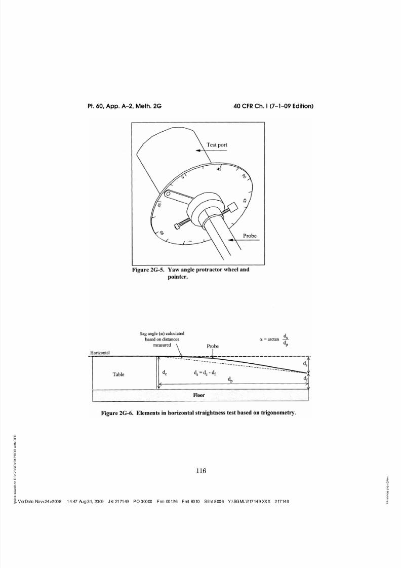
7/28/2019 40cfr60AppA-2
http://slidepdf.com/reader/full/40cfr60appa-2 27/70
116
40 CFR Ch. I (7–1–09 Edition)Pt. 60, App. A–2, Meth. 2G
VerDate Nov<24>2008 14:47 Aug 31, 2009 Jkt 217149 PO 00000 Frm 00126 Fmt 8010 Sfmt 8006 Y:\SGML\217149.XXX 217149

7/28/2019 40cfr60AppA-2
http://slidepdf.com/reader/full/40cfr60appa-2 28/70
117
Environmental Protection Agency Pt. 60, App. A–2, Meth. 2G
VerDate Nov<24>2008 14:47 Aug 31, 2009 Jkt 217149 PO 00000 Frm 00127 Fmt 8010 Sfmt 8006 Y:\SGML\217149.XXX 217149

7/28/2019 40cfr60AppA-2
http://slidepdf.com/reader/full/40cfr60appa-2 29/70
118
40 CFR Ch. I (7–1–09 Edition)Pt. 60, App. A–2, Meth. 2G
VerDate Nov<24>2008 14:47 Aug 31, 2009 Jkt 217149 PO 00000 Frm 00128 Fmt 8010 Sfmt 8006 Y:\SGML\217149.XXX 217149

7/28/2019 40cfr60AppA-2
http://slidepdf.com/reader/full/40cfr60appa-2 30/70
119
Environmental Protection Agency Pt. 60, App. A–2, Meth. 2G
VerDate Nov<24>2008 14:47 Aug 31, 2009 Jkt 217149 PO 00000 Frm 00129 Fmt 8010 Sfmt 8006 Y:\SGML\217149.XXX 217149

7/28/2019 40cfr60AppA-2
http://slidepdf.com/reader/full/40cfr60appa-2 31/70
120
40 CFR Ch. I (7–1–09 Edition)Pt. 60, App. A–2, Meth. 2G
VerDate Nov<24>2008 14:47 Aug 31, 2009 Jkt 217149 PO 00000 Frm 00130 Fmt 8010 Sfmt 8006 Y:\SGML\217149.XXX 217149

7/28/2019 40cfr60AppA-2
http://slidepdf.com/reader/full/40cfr60appa-2 32/70
121
Environmental Protection Agency Pt. 60, App. A–2, Meth. 2G
VerDate Nov<24>2008 14:47 Aug 31, 2009 Jkt 217149 PO 00000 Frm 00131 Fmt 8010 Sfmt 8006 Y:\SGML\217149.XXX 217149

7/28/2019 40cfr60AppA-2
http://slidepdf.com/reader/full/40cfr60appa-2 33/70
122
40 CFR Ch. I (7–1–09 Edition)Pt. 60, App. A–2, Meth. 2G
VerDate Nov<24>2008 14:47 Aug 31, 2009 Jkt 217149 PO 00000 Frm 00132 Fmt 8010 Sfmt 8006 Y:\SGML\217149.XXX 217149

7/28/2019 40cfr60AppA-2
http://slidepdf.com/reader/full/40cfr60appa-2 34/70
123
Environmental Protection Agency Pt. 60, App. A–2, Meth. 2G
VerDate Nov<24>2008 14:47 Aug 31, 2009 Jkt 217149 PO 00000 Frm 00133 Fmt 8010 Sfmt 8006 Y:\SGML\217149.XXX 217149

7/28/2019 40cfr60AppA-2
http://slidepdf.com/reader/full/40cfr60appa-2 35/70
124
40 CFR Ch. I (7–1–09 Edition)Pt. 60, App. A–2, Meth. 2G
VerDate Nov<24>2008 14:47 Aug 31, 2009 Jkt 217149 PO 00000 Frm 00134 Fmt 8010 Sfmt 8006 Y:\SGML\217149.XXX 217149

7/28/2019 40cfr60AppA-2
http://slidepdf.com/reader/full/40cfr60appa-2 36/70
125
Environmental Protection Agency Pt. 60, App. A–2, Meth. 2G
VerDate Nov<24>2008 14:47 Aug 31, 2009 Jkt 217149 PO 00000 Frm 00135 Fmt 8010 Sfmt 8006 Y:\SGML\217149.XXX 217149

7/28/2019 40cfr60AppA-2
http://slidepdf.com/reader/full/40cfr60appa-2 37/70
126
40 CFR Ch. I (7–1–09 Edition)Pt. 60, App. A–2, Meth. 2G
VerDate Nov<24>2008 14:47 Aug 31, 2009 Jkt 217149 PO 00000 Frm 00136 Fmt 8010 Sfmt 8006 Y:\SGML\217149.XXX 217149

7/28/2019 40cfr60AppA-2
http://slidepdf.com/reader/full/40cfr60appa-2 38/70
127
Environmental Protection Agency Pt. 60, App. A–2, Meth. 2G
VerDate Nov<24>2008 14:47 Aug 31, 2009 Jkt 217149 PO 00000 Frm 00137 Fmt 8010 Sfmt 8006 Y:\SGML\217149.XXX 217149

7/28/2019 40cfr60AppA-2
http://slidepdf.com/reader/full/40cfr60appa-2 39/70
128
40 CFR Ch. I (7–1–09 Edition)Pt. 60, App. A–2, Meth. 2H
METHOD 2H—DETERMINATION OF STACK GAS VELOCITY TAKING INTO ACCOUNT VELOCITY DECAY NEAR THE STACK WALL
1.0 Scope and Application
1.1 This method is applicable in conjunc-tion with Methods 2, 2F, and 2G (40 CFR Part60, Appendix A) to account for velocity decaynear the wall in circular stacks and ducts.
1.2 This method is not applicable for test-ing stacks and ducts less than 3.3 ft (1.0 m)in diameter.
1.3 Data Quality Objectives. Adherence tothe requirements of this method will en-hance the quality of the data obtained fromair pollutant sampling methods.
2.0 Summary of Method
2.1 A wall effects adjustment factor is de-termined. It is used to adjust the averagestack gas velocity obtained under Method 2,2F, or 2G of this appendix to take into ac-count velocity decay near the stack or ductwall.
2.2 The method contains two possible pro-cedures: a calculational approach which de-rives an adjustment factor from velocitymeasurements and a default procedure whichassigns a generic adjustment factor based onthe construction of the stack or duct.
2.2.1 The calculational procedure derivesa wall effects adjustment factor from veloc-ity measurements taken using Method 2, 2F,or 2G at 16 (or more) traverse points speci-fied under Method 1 of this appendix and atotal of eight (or more) wall effects traversepoints specified under this method. Thecalculational procedure based on velocitymeasurements is not applicable for hori-zontal circular ducts where build-up of par-ticulate matter or other material in the bot-tom of the duct is present.
2.2.2 A default wall effects adjustmentfactor of 0.9900 for brick and mortar stacksand 0.9950 for all other types of stacks andducts may be used without taking wall ef-fects measurements in a stack or duct.
2.3 When the calculational procedure isconducted as part of a relative accuracy testaudit (RATA) or other multiple-run test pro-cedure, the wall effects adjustment factorderived from a single traverse (i.e., singleRATA run) may be applied to all runs of thesame RATA without repeating the wall ef-
fects measurements. Alternatively, wall ef-fects adjustment factors may be derived forseveral traverses and an average wall effectsadjustment factor applied to all runs of thesame RATA.
3.0 Definitions.
3.1 Complete wall effects traverse means atraverse in which measurements are takenat d rem (see section 3.3) and at 1-in. intervalsin each of the four Method 1 equal-area sec-tors closest to the wall, beginning not far-
ther than 4 in. (10.2 cm) from the wall andextending either (1) across the entire widthof the Method 1 equal-area sector or (2) forstacks or ducts where this width exceeds 12in. (30.5 cm) (i.e., stacks or ducts greaterthan or equal to 15.6 ft [4.8 m] in diameter),to a distance of not less than 12 in. (30.5 cm)from the wall. Note: Because this methodspecifies that measurements must be takenat whole number multiples of 1 in. from astack or duct wall, for clarity numericalquantities in this method are expressed inEnglish units followed by metric units in pa-rentheses. To enhance readability, hyphen-ated terms such as ‘‘1-in. intervals’’ or ‘‘1-in.incremented,’’ are expressed in English units
only.3.2 dlast Depending on context, dlast means
either (1) the distance from the wall of thelast 1-in. incremented wall effects traversepoint or (2) the traverse point located at thatdistance (see Figure 2H–2).
3.3 drem Depending on context, drem meanseither (1) the distance from the wall of thecentroid of the area between dlast and the in-terior edge of the Method 1 equal-area sectorclosest to the wall or (2) the traverse pointlocated at that distance (see Figure 2H–2).
3.4 ‘‘May,’’ ‘‘Must,’’ ‘‘Shall,’’ ‘‘Should,’’ andthe imperative form of verbs.
3.4.1 ‘‘May’’ is used to indicate that a pro-vision of this method is optional.
3.4.2 ‘‘Must,’’ ‘‘Shall,’’ and the imperativeform of verbs (such as ‘‘record’’ or ‘‘enter’’)are used to indicate that a provision of this
method is mandatory.3.4.3 ‘‘Should’’ is used to indicate that a
provision of this method is not mandatorybut is highly recommended as good practice.
3.5 Method 1 refers to 40 CFR part 60, ap-pendix A, ‘‘Method 1—Sample and velocitytraverses for stationary sources.’’
3.6 Method 1 exterior equal-area sector and
Method 1 equal-area sector closest to the wall
mean any one of the four equal-area sectorsthat are closest to the wall for a circularstack or duct laid out in accordance withsection 2.3.1 of Method 1 (see Figure 2H–1).
3.7 Method 1 interior equal-area sector
means any of the equal-area sectors otherthan the Method 1 exterior equal-area sec-tors (as defined in section 3.6) for a circularstack or duct laid out in accordance withsection 2.3.1 of Method 1 (see Figure 2H–1).
3.8 Method 1 traverse point and Method 1equal-area traverse point mean a traversepoint located at the centroid of an equal-area sector of a circular stack laid out in ac-cordance with section 2.3.1 of Method 1.
3.9 Method 2 refers to 40 CFR part 60, ap-pendix A, ‘‘Method 2—Determination of stack gas velocity and volumetric flow rate(Type S pitot tube).’’
3.10 Method 2F refers to 40 CFR part 60,appendix A, ‘‘Method 2F—Determination of stack gas velocity and volumetric flow ratewith three-dimensional probes.’’
VerDate Nov<24>2008 14:47 Aug 31, 2009 Jkt 217149 PO 00000 Frm 00138 Fmt 8010 Sfmt 8002 Y:\SGML\217149.XXX 217149

7/28/2019 40cfr60AppA-2
http://slidepdf.com/reader/full/40cfr60appa-2 40/70
129
Environmental Protection Agency Pt. 60, App. A–2, Meth. 2H
3.11 Method 2G refers to 40 CFR part 60,appendix A, ‘‘Method 2G—Determination of stack gas velocity and volumetric flow ratewith two-dimensional probes.’’
3.12 1-in. incremented wall effects traverse
point means any of the wall effects traversepoints that are located at 1-in. intervals, i.e.,traverse points d1 through dlast (see Figure2H–2).
3.13 Partial wall effects traverse means atraverse in which measurements are takenat fewer than the number of traverse pointsrequired for a ‘‘complete wall effects tra-verse’’ (as defined in section 3.1), but aretaken at a minimum of two traverse pointsin each Method 1 equal-area sector closest tothe wall, as specified in section 8.2.2.
3.14 Relative accuracy test audit (RATA) isa field test procedure performed in a stack orduct in which a series of concurrent meas-urements of the same stack gas stream istaken by a reference method and an installedmonitoring system. A RATA usually consistsof series of 9 to 12 sets of such concurrentmeasurements, each of which is referred toas a RATA run. In a volumetric flow RATA,each reference method run consists of a com-plete traverse of the stack or duct.
3.15 Wall effects-unadjusted average velocity
means the average stack gas velocity, notaccounting for velocity decay near the wall,as determined in accordance with Method 2,2F, or 2G for a Method 1 traverse consistingof 16 or more points.
3.16 Wall effects-adjusted average velocitymeans the average stack gas velocity, takinginto account velocity decay near the wall, ascalculated from measurements at 16 or moreMethod 1 traverse points and at the addi-tional wall effects traverse points specifiedin this method.
3.17 Wall effects traverse point means a tra-verse point located in accordance with sec-tions 8.2.2 or 8.2.3 of this method.
4.0 Interferences [Reserved]
5.0 Safety
5.1 This method may involve hazardousmaterials, operations, and equipment. Thismethod does not purport to address all of thehealth and safety considerations associatedwith its use. It is the responsibility of the
user of this method to establish appropriatehealth and safety practices and to determinethe applicability of occupational health andsafety regulatory requirements prior to per-forming this method.
6.0 Equipment and Supplies
6.1 The provisions pertaining to equip-ment and supplies in the method that is usedto take the traverse point measurements
(i.e., Method 2, 2F, or 2G) are applicableunder this method.
7.0 Reagents and Standards [Reserved]
8.0 Sample Collection and Analysis
8.1 Default Wall Effects Adjustment Fac-tors. A default wall effects adjustment factorof 0.9900 for brick and mortar stacks and0.9950 for all other types of stacks and ductsmay be used without conducting the fol-lowing procedures.
8.2 Traverse Point Locations. Determinethe location of the Method 1 traverse pointsin accordance with section 8.2.1 and the loca-tion of the traverse points for either a par-tial wall effects traverse in accordance withsection 8.2.2 or a complete wall effects tra-verse in accordance with section 8.2.3.
8.2.1 Method 1 equal-area traverse pointlocations. Determine the location of theMethod 1 equal-area traverse points for atraverse consisting of 16 or more pointsusing Table 1–2 (Location of Traverse Pointsin Circular Stacks) of Method 1.
8.2.2 Partial wall effects traverse. For apartial wall effects traverse, measurementsmust be taken at a minimum of the fol-lowing two wall effects traverse point loca-tions in all four Method 1 equal-area sectorsclosest to the wall: (1) 1 in. (2.5 cm) from thewall (except as provided in section 8.2.2.1)and (2) drem, as determined using Equation2H–1 or 2H–2 (see section 8.2.2.2).
8.2.2.1 If the probe cannot be positioned at
1 in. (2.5 cm) from the wall (e.g., because of insufficient room to withdraw the probeshaft) or if velocity pressure cannot be de-tected at 1 in. (2.5 cm) from the wall (for anyreason other than build-up of particulatematter in the bottom of a duct), take meas-urements at the 1-in. incremented wall ef-fects traverse point closest to the wall wherethe probe can be positioned and velocitypressure can be detected.
8.2.2.2 Calculate the distance of drem fromthe wall to within ±1 ⁄ 4 in. (6.4 mm) usingEquation 2H–1 or Equation 2H–2 (for a 16-point traverse).
d d Eqlast b≤ . 2H-3
Where:
r=the stack or duct radius determined from
direct measurement of the stack or ductdiameter in accordance with section 8.6 of Method 2F or Method 2G, in. (cm);
p=the number of Method 1 equal-area tra-verse points on a diameter, p ≥ 8 (e.g., fora 16-point traverse, p=8); dlast and drem aredefined in sections 3.2 and 3.3 respectively,in. (cm).
For a 16-point Method 1 traverse, Equation2H–1 becomes:
VerDate Nov<24>2008 14:47 Aug 31, 2009 Jkt 217149 PO 00000 Frm 00139 Fmt 8010 Sfmt 8003 Y:\SGML\217149.XXX 217149

7/28/2019 40cfr60AppA-2
http://slidepdf.com/reader/full/40cfr60appa-2 41/70
130
40 CFR Ch. I (7–1–09 Edition)Pt. 60, App. A–2, Meth. 2H
d r r rd drem last last= − − +7
8
1
2
2 2 Eq. 2H-2
8.2.2.3 Measurements may be taken at anynumber of additional wall effects traversepoints, with the following provisions.
(a) dlast must not be closer to the center of the stack or duct than the distance of the in-terior edge (boundary), db, of the Method 1equal-area sector closest to the wall (seeFigure 2H–2 or 2H–3). That is,
Where:
d rp
Eqb = − −⎛
⎝ ⎜⎞
⎠ ⎟ 1 1
24. 2H-
Table 2H–1 shows db as a function of thestack or duct radius, r, for traverses rangingfrom 16 to 48 points (i.e., for values of p rang-ing from 8 to 24).
(b) Each point must be located at a dis-tance that is a whole number (e.g., 1, 2, 3)multiple of 1 in. (2.5 cm).
(c) Points do not have to be located at con-secutive 1-in. intervals. That is, one or more1-in. incremented points may be skipped. Forexample, it would be acceptable for points tobe located at 1 in. (2.5 cm), 3 in. (7.6 cm), 5 in.(12.7 cm), dlast , and drem; or at 1 in. (2.5 cm), 2in. (5.1 cm), 4 in. (10.2 cm), 7 in. (17.8 cm), dlast ,
and drem. Follow the instructions in section8.7.1.2 of this method for recording resultsfor wall effects traverse points that areskipped. It should be noted that the full ex-tent of velocity decay may not be accountedfor if measurements are not taken at all 1-in.incremented points close to the wall.
8.2.3 Complete wall effects traverse. For acomplete wall effects traverse, measure-ments must be taken at the following pointsin all four Method 1 equal-area sectors clos-est to the wall.
(a) The 1-in. incremented wall effects tra-verse point closest to the wall where theprobe can be positioned and velocity can bedetected, but no farther than 4 in. (10.2 cm)from the wall.
(b) Every subsequent 1-in. incrementedwall effects traverse point out to the interior
edge of the Method 1 equal-area sector or to12 in. (30.5 cm) from the wall, whichevercomes first. Note: In stacks or ducts with di-ameters greater than 15.6 ft (4.8 m) the inte-rior edge of the Method 1 equal-area sector isfarther from the wall than 12 in. (30.5 cm).
(c) drem, as determined using Equation 2H– 1 or 2H–2 (as applicable). Note: For a com-plete traverse of a stack or duct with a di-ameter less than 16.5 ft (5.0 m), the distancebetween drem and dlast is less than or equal to1 ⁄ 2 in. (12.7 mm). As discussed in section8.2.4.2, when the distance between drem and
dlast is less than or equal to 1 ⁄ 2 in. (12.7 mm),
the velocity measured at dlast may be used fordrem. Thus, it is not necessary to calculate
the distance of drem or to take measurements
at drem when conducting a complete traverseof a stack or duct with a diameter less than
16.5 ft (5.0 m).
8.2.4 Special considerations. The fol-
lowing special considerations apply when the
distance between traverse points is less thanor equal to 1 ⁄ 2 in. (12.7 mm).
8.2.4.1 A wall effects traverse point and
the Method 1 traverse point. If the distancebetween a wall effects traverse point and the
Method 1 traverse point is less than or equal
to 1 ⁄ 2 in. (12.7 mm), taking measurements atboth points is allowed but not required or
recommended; if measurements are taken at
only one point, take the measurements atthe point that is farther from the wall anduse the velocity obtained at that point asthe value for both points (see sections 8.2.3and 9.2 for related requirements).
8.2.4.2 drem and dlast. If the distance be-tween drem and dlast is less than or equal to 1 ⁄ 2 in. (12.7 mm), taking measurements at drem isallowed but not required or recommended; if measurements are not taken at drem, the
measured velocity value at dlast must be usedas the value for both dlast and drem.
8.3 Traverse Point Sampling Order andProbe Selection. Determine the samplingorder of the Method 1 and wall effects tra-verse points and select the appropriate probefor the measurements, taking into accountthe following considerations.
8.3.1 Traverse points on any radius maybe sampled in either direction (i.e., from thewall toward the center of the stack or duct,or vice versa).
8.3.2 To reduce the likelihood of velocityvariations during the time of the traverseand the attendant potential impact on thewall effects-adjusted and unadjusted averagevelocities, the following provisions of thismethod shall be met.
8.3.2.1 Each complete set of Method 1 andwall effects traverse points accessed fromthe same port shall be sampled withoutinterruption. Unless traverses are performedsimultaneously in all ports using separateprobes at each port, this provision disallowsfirst sampling all Method 1 points at allports and then sampling all the wall effectspoints.
8.3.2.2 The entire integrated Method 1 andwall effects traverse across all test portsshall be as short as practicable, consistentwith the measurement system response time
VerDate Nov<24>2008 14:47 Aug 31, 2009 Jkt 217149 PO 00000 Frm 00140 Fmt 8010 Sfmt 8002 Y:\SGML\217149.XXX 217149

7/28/2019 40cfr60AppA-2
http://slidepdf.com/reader/full/40cfr60appa-2 42/70
131
Environmental Protection Agency Pt. 60, App. A–2, Meth. 2H
(see section 8.4.1.1) and sampling (see section8.4.1.2) provisions of this method.
8.3.3 It is recommended but not requiredthat in each Method 1 equal-area sector clos-est to the wall, the Method 1 equal-area tra-verse point should be sampled in sequencebetween the adjacent wall effects traversepoints. For example, for the traverse pointconfiguration shown in Figure 2H–2, it is rec-ommended that the Method 1 equal-area tra-verse point be sampled between dlast and drem.In this example, if the traverse is conductedfrom the wall toward the center of the stackor duct, it is recommended that measure-ments be taken at points in the followingorder: d1, d2, dlast, the Method 1 traverse
point, drem, and then at the traverse points inthe three Method 1 interior equal-area sec-tors.
8.3.4 The same type of probe must be usedto take measurements at all Method 1 andwall effects traverse points. However, dif-ferent copies of the same type of probe maybe used at different ports (e.g., Type S probe1 at port A, Type S probe 2 at port B) or atdifferent traverse points accessed from a par-ticular port (e.g., Type S probe 1 for Method1 interior traverse points accessed from portA, Type S probe 2 for wall effects traversepoints and the Method 1 exterior traversepoint accessed from port A). The identifica-tion number of the probe used to obtainmeasurements at each traverse point mustbe recorded.
8.4 Measurements at Method 1 and Wall
Effects Traverse Points. Conduct measure-ments at Method 1 and wall effects traversepoints in accordance with Method 2, 2F, or2G and in accordance with the provisions of the following subsections (some of which areincluded in Methods 2F and 2G but not inMethod 2), which are particularly importantfor wall effects testing.
8.4.1 Probe residence time at wall effectstraverse points. Due to the steep tempera-ture and pressure gradients that can occurclose to the wall, it is very important for theprobe residence time (i.e., the total timespent at a traverse point) to be long enoughto ensure collection of representative tem-perature and pressure measurements. Theprovisions of Methods 2F and 2G in the fol-lowing subsections shall be observed.
8.4.1.1 System response time. Determine
the response time of each probe measure-ment system by inserting and positioningthe ‘‘cold’’ probe (at ambient temperatureand pressure) at any Method 1 traversepoint. Read and record the probe differentialpressure, temperature, and elapsed time at15-second intervals until stable readings forboth pressure and temperature are achieved.The response time is the longer of these twoelapsed times. Record the response time.
8.4.1.2 Sampling. At the start of testing ineach port (i.e., after a probe has been in-serted into the stack gas stream), allow at
least the response time to elapse before be-ginning to take measurements at the firsttraverse point accessed from that port. Pro-vided that the probe is not removed from thestack gas stream, measurements may betaken at subsequent traverse points accessedfrom the same test port without waitingagain for the response time to elapse.
8.4.2 Temperature measurement for walleffects traverse points. Either (1) take tem-perature measurements at each wall effectstraverse point in accordance with the appli-cable provisions of Method 2, 2F, or 2G; or (2)use the temperature measurement at theMethod 1 traverse point closest to the wallas the temperature measurement for all thewall effects traverse points in the cor-responding equal-area sector.
8.4.3 Non-detectable velocity pressure atwall effects traverse points. If the probe can-not be positioned at a wall effects traversepoint or if no velocity pressure can be de-tected at a wall effects point, measurementsshall be taken at the first subsequent walleffects traverse point farther from the wallwhere velocity can be detected. Follow theinstructions in section 8.7.1.2 of this methodfor recording results for wall effects traversepoints where velocity pressure cannot be de-tected. It should be noted that the full ex-tent of velocity decay may not be accountedfor if measurements are not taken at the 1-in. incremented wall effects traverse pointsclosest to the wall.
8.5 Data Recording. For each wall effectsand Method 1 traverse point where measure-ments are taken, record all pressure, tem-perature, and attendant measurements pre-scribed in section 3 of Method 2 or section 8.0of Method 2F or 2G, as applicable.
8.6 Point Velocity Calculation. For eachwall effects and Method 1 traverse point, cal-culate the point velocity value (vi) in accord-ance with sections 12.1 and 12.2 of Method 2Ffor tests using Method 2F and in accordancewith sections 12.1 and 12.2 of Method 2G fortests using Method 2 and Method 2G. (Notethat the term (vi) in this method correspondsto the term (va(i)) in Methods 2F and 2G.)When the equations in the indicated sectionsof Method 2G are used in deriving point ve-locity values for Method 2 tests, set thevalue of the yaw angles appearing in theequations to 0°.
8.7 Tabulating Calculated Point VelocityValues for Wall Effects Traverse Points.Enter the following values in a hardcopy orelectronic form similar to Form 2H–1 (for 16-point Method 1 traverses) or Form 2H–2 (forMethod 1 traverses consisting of more than16 points). A separate form must be com-pleted for each of the four Method 1 equal-area sectors that are closest to the wall.
(a) Port ID (e.g., A, B, C, or D)
(b) Probe type
(c) Probe ID
VerDate Nov<24>2008 14:47 Aug 31, 2009 Jkt 217149 PO 00000 Frm 00141 Fmt 8010 Sfmt 8002 Y:\SGML\217149.XXX 217149

7/28/2019 40cfr60AppA-2
http://slidepdf.com/reader/full/40cfr60appa-2 43/70
132
40 CFR Ch. I (7–1–09 Edition)Pt. 60, App. A–2, Meth. 2H
(d) Stack or duct diameter in ft (m) (deter-mined in accordance with section 8.6 of Method 2F or Method 2G)
(e) Stack or duct radius in in. (cm)(f) Distance from the wall of wall effects
traverse points at 1-in. intervals, in ascend-ing order starting with 1 in. (2.5 cm) (columnA of Form 2H–1 or 2H–2)
(g) Point velocity values (vd ) for 1-in. in-cremented traverse points (see section 8.7.1),including dlast (see section 8.7.2)
(h) Point velocity value (vdrem) at drem (seesection 8.7.3).
8.7.1 Point velocity values at wall effectstraverse points other than dlast . For every 1-in. incremented wall effects traverse point
other than dlast , enter in column B of Form2H–1 or 2H–2 either the velocity measured atthe point (see section 8.7.1.1) or the velocitymeasured at the first subsequent traversepoint farther from the wall (see section8.7.1.2). A velocity value must be entered incolumn B of Form 2H–1 or 2H–2 for every 1-in. incremented traverse point from d1 (rep-resenting the wall effects traverse point 1 in.[2.5 cm] from the wall) to dlast .
8.7.1.1 For wall effects traverse pointswhere the probe can be positioned and veloc-ity pressure can be detected, enter the valueobtained in accordance with section 8.6.
8.7.1.2 For wall effects traverse pointsthat were skipped [see section 8.2.2.3(c)] andfor points where the probe cannot be posi-tioned or where no velocity pressure can bedetected, enter the value obtained at the
first subsequent traverse point farther fromthe wall where velocity pressure was de-tected and measured and follow the enteredvalue with a ‘‘flag,’’ such as the notation‘‘NM,’’ to indicate that ‘‘no measurements’’were actually taken at this point.
8.7.2 Point velocity value at dlast . For dlast ,enter in column B of Form 2H–1 or 2H–2 themeasured value obtained in accordance withsection 8.6.
8.7.3 Point velocity value (vdrem) at drem.Enter the point velocity value obtained atdrem in column G of row 4a in Form 2H–1 or2H–2. If the distance between drem and dlast isless than or equal to 1 ⁄ 2 in. (12.7 mm), themeasured velocity value at dlast may be usedas the value at drem (see section 8.2.4.2).
9.0 Quality Control.
9.1 Particulate Matter Build-up in Hori-zontal Ducts. Wall effects testing of hori-zontal circular ducts should be conductedonly if build-up of particulate matter orother material in the bottom of the duct isnot present.
9.2 Verifying Traverse Point Distances. Intaking measurements at wall effects tra-verse points, it is very important for theprobe impact pressure port to be positionedas close as practicable to the traverse pointlocations in the gas stream. For this reason,before beginning wall effects testing, it is
important to calculate and record the tra-verse point positions that will be marked oneach probe for each port, taking into accountthe distance that each port nipple (or probemounting flange for automated probes) ex-tends out of the stack and any extension of the port nipple (or mounting flange) into thegas stream. To ensure that traverse point po-sitions are properly identified, the followingprocedures should be performed on eachprobe used.
9.2.1 Manual probes. Mark the probe in-sertion distance of the wall effects and Meth-od 1 traverse points on the probe sheath sothat when a mark is aligned with the outsideface of the stack port, the probe impact portis located at the calculated distance of thetraverse point from the stack inside wall.The use of different colored marks is rec-ommended for designating the wall effectsand Method 1 traverse points. Before thefirst use of each probe, check to ensure thatthe distance of each mark from the center of the probe impact pressure port agrees withthe previously calculated traverse point po-sitions to within ±1 ⁄ 4 in. (6.4 mm).
9.2.2 Automated probe systems. For auto-mated probe systems that mechanically po-sition the probe head at prescribed traversepoint positions, activate the system with theprobe assemblies removed from the testports and sequentially extend the probes tothe programmed location of each wall effectstraverse point and the Method 1 traversepoints. Measure the distance between the
center of the probe impact pressure port andthe inside of the probe assembly mountingflange for each traverse point. The measureddistances must agree with the previouslycalculated traverse point positions to within±1 ⁄ 4 in. (6.4 mm).
9.3 Probe Installation. Properly sealingthe port area is particularly important intaking measurements at wall effects tra-verse points. For testing involving manualprobes, the area between the probe sheathand the port should be sealed with a tightlyfitting flexible seal made of an appropriatematerial such as heavy cloth so that leakageis minimized. For automated probe systems,the probe assembly mounting flange areashould be checked to verify that there is noleakage.
9.4 Velocity Stability. This method
should be performed only when the averagegas velocity in the stack or duct is relativelyconstant over the duration of the test. If theaverage gas velocity changes significantlyduring the course of a wall effects test, thetest results should be discarded.
10.0 Calibration
10.1 The calibration coefficient(s) orcurves obtained under Method 2, 2F, or 2Gand used to perform the Method 1 traverseare applicable under this method.
VerDate Nov<24>2008 14:47 Aug 31, 2009 Jkt 217149 PO 00000 Frm 00142 Fmt 8010 Sfmt 8002 Y:\SGML\217149.XXX 217149
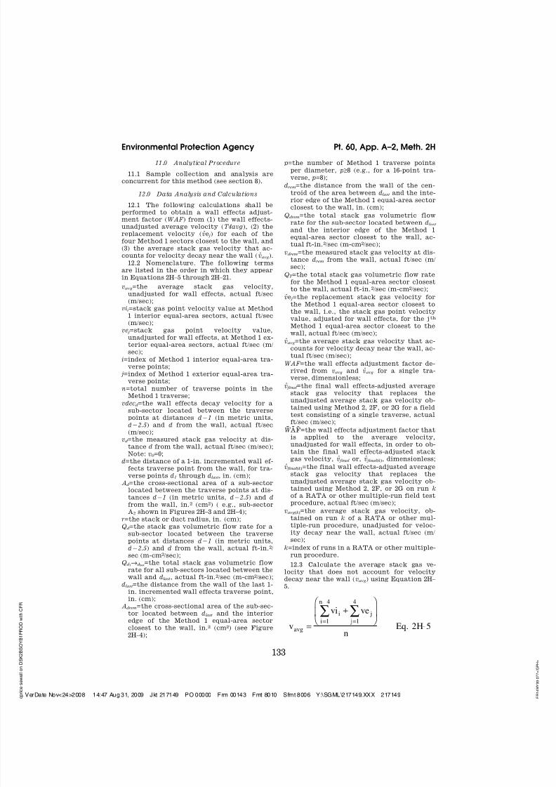
7/28/2019 40cfr60AppA-2
http://slidepdf.com/reader/full/40cfr60appa-2 44/70
133
Environmental Protection Agency Pt. 60, App. A–2, Meth. 2H
11.0 Analytical Procedure
11.1 Sample collection and analysis areconcurrent for this method (see section 8).
12.0 Data Analysis and Calculations
12.1 The following calculations shall beperformed to obtain a wall effects adjust-ment factor (WAF ) from (1) the wall effects-unadjusted average velocity (T4avg), (2) thereplacement velocity (v e j) for each of thefour Method 1 sectors closest to the wall, and(3) the average stack gas velocity that ac-counts for velocity decay near the wall (v avg).
12.2 Nomenclature. The following termsare listed in the order in which they appear
in Equations 2H–5 through 2H–21.
vavg=the average stack gas velocity,unadjusted for wall effects, actual ft/sec(m/sec);
vii=stack gas point velocity value at Method1 interior equal-area sectors, actual ft/sec(m/sec);
ve j=stack gas point velocity value,unadjusted for wall effects, at Method 1 ex-terior equal-area sectors, actual ft/sec (m/sec);
i=index of Method 1 interior equal-area tra-verse points;
j =index of Method 1 exterior equal-area tra-verse points;
n=total number of traverse points in theMethod 1 traverse;
vdecd =the wall effects decay velocity for asub-sector located between the traversepoints at distances d¥1 (in metric units,d¥2.5) and d from the wall, actual ft/sec(m/sec);
vd =the measured stack gas velocity at dis-tance d from the wall, actual ft/sec (m/sec);Note: v0=0;
d=the distance of a 1-in. incremented wall ef-fects traverse point from the wall, for tra-verse points d1 through dlast , in. (cm);
Ad =the cross-sectional area of a sub-sectorlocated between the traverse points at dis-tances d¥1 (in metric units, d¥2.5) and d
from the wall, in.2 (cm2) ( e.g., sub-sectorA2 shown in Figures 2H–3 and 2H–4);
r=the stack or duct radius, in. (cm);
Qd =the stack gas volumetric flow rate for asub-sector located between the traversepoints at distances d¥1 (in metric units,d¥2.5) and d from the wall, actual ft-in.2/sec (m-cm2/sec);
Qd 1→d last=the total stack gas volumetric flowrate for all sub-sectors located between thewall and dlast , actual ft-in.2/sec (m-cm2/sec);
dlast =the distance from the wall of the last 1-in. incremented wall effects traverse point,in. (cm);
Adrem=the cross-sectional area of the sub-sec-tor located between dlast and the interioredge of the Method 1 equal-area sectorclosest to the wall, in.2 (cm2) (see Figure2H–4);
p=the number of Method 1 traverse points
per diameter, p≥8 (e.g., for a 16-point tra-
verse, p=8);
drem=the distance from the wall of the cen-
troid of the area between dlast and the inte-
rior edge of the Method 1 equal-area sectorclosest to the wall, in. (cm);
Qdrem=the total stack gas volumetric flow
rate for the sub-sector located between dlast and the interior edge of the Method 1equal-area sector closest to the wall, ac-tual ft-in.2/sec (m-cm2/sec);
vdrem=the measured stack gas velocity at dis-tance drem from the wall, actual ft/sec (m/sec);
QT =the total stack gas volumetric flow ratefor the Method 1 equal-area sector closestto the wall, actual ft-in.2/sec (m-cm2/sec);
v e j=the replacement stack gas velocity forthe Method 1 equal-area sector closest tothe wall, i.e., the stack gas point velocityvalue, adjusted for wall effects, for the jth Method 1 equal-area sector closest to thewall, actual ft/sec (m/sec);
v avg=the average stack gas velocity that ac-counts for velocity decay near the wall, ac-tual ft/sec (m/sec);
WAF =the wall effects adjustment factor de-rived from vavg and v avg for a single tra-verse, dimensionless;
v final=the final wall effects-adjusted averagestack gas velocity that replaces theunadjusted average stack gas velocity ob-tained using Method 2, 2F, or 2G for a field
test consisting of a single traverse, actualft/sec (m/sec);
W ¯ A F =the wall effects adjustment factor thatis applied to the average velocity,unadjusted for wall effects, in order to ob-tain the final wall effects-adjusted stackgas velocity, v final or, v final(k ), dimensionless;
v final(k )=the final wall effects-adjusted averagestack gas velocity that replaces theunadjusted average stack gas velocity ob-tained using Method 2, 2F, or 2G on run k
of a RATA or other multiple-run field testprocedure, actual ft/sec (m/sec);
vavg(k )=the average stack gas velocity, ob-tained on run k of a RATA or other mul-tiple-run procedure, unadjusted for veloc-ity decay near the wall, actual ft/sec (m/sec);
k=index of runs in a RATA or other multiple-run procedure.
12.3 Calculate the average stack gas ve-locity that does not account for velocitydecay near the wall (vavg) using Equation 2H– 5.
v
vi ve
nEqavg
i j
ji
n
=
+⎛
⎝ ⎜
⎞
⎠ ⎟
==
−
∑∑1
4
1
4
5. 2H-
VerDate Nov<24>2008 14:47 Aug 31, 2009 Jkt 217149 PO 00000 Frm 00143 Fmt 8010 Sfmt 8006 Y:\SGML\217149.XXX 217149

7/28/2019 40cfr60AppA-2
http://slidepdf.com/reader/full/40cfr60appa-2 45/70
134
40 CFR Ch. I (7–1–09 Edition)Pt. 60, App. A–2, Meth. 2H
(Note that vavg in Equation 2H–5 is the sameas v(a)avg in Equations 2F–9 and 2G–8 in Meth-ods 2F and 2G, respectively.)
For a 16-point traverse, Equation 2H–5 maybe written as follows:
v
vi ve
Eqavg
i j
ji=
+⎛
⎝ ⎜
⎞
⎠ ⎟
==∑∑
1
4
1
12
16. 2H-6
12.4 Calculate the replacement velocity,v e j, for each of the four Method 1 equal-areasectors closest to the wall using the proce-dures described in sections 12.4.1 through
12.4.8. Forms 2H–1 and 2H–2 provide sampletables that may be used in either hardcopyor spreadsheet format to perform the cal-culations described in sections 12.4.1 through12.4.8. Forms 2H–3 and 2H–4 provide examples
of Form 2H–1 filled in for partial and com-
plete wall effects traverses.
12.4.1 Calculate the average velocity (des-
ignated the ‘‘decay velocity,’’ vdecd) for each
sub-sector located between the wall and dlast
(see Figure 2H–3) using Equation 2H–7.
vdecv v
Eqdd d=
+−1
2. 2H-7
For each line in column A of Form 2H–1 or
2H–2 that contains a value of d, enter the
corresponding calculated value of vdecd in
column C.
12.4.2 Calculate the cross-sectional area
between the wall and the first 1-in. incre-mented wall effects traverse point and be-
tween successive 1-in. incremented wall ef-
fects traverse points, from the wall to dlast
(see Figure 2H–3), using Equation 2H–8.
A r d r d Eqd = − +( ) − −( )1
41
1
4
2 2π π . 2H-8
For each line in column A of Form 2H–1 or
2H–2 that contains a value of d, enter the
value of the expression 1 ⁄ 4 π(r¥d+1)2 in col-
umn D, the value of the expression 1 ⁄ 4 π(r¥d)2
in column E, and the value of Ad in column
F. Note that Equation 2H–8 is designed for
use only with English units (in.). If metricunits (cm) are used, the first term, 1 ⁄ 4
π(r¥d+1)2, must be changed to 1 ⁄ 4 π(r¥d+2.5)2.
This change must also be made in column D
of Form 2H–1 or 2H–2.
12.4.3 Calculate the volumetric flow
through each cross-sectional area derived in
section 12.4.2 by multiplying the values of vdecd , derived according to section 12.4.1, bythe cross-sectional areas derived in section12.4.2 using Equation 2H–9.
Q vdec A Eqd d d= × . 2H-9
For each line in column A of Form 2H–1 or2H–2 that contains a value of d, enter thecorresponding calculated value of Qd in col-umn G.
12.4.4 Calculate the total volumetric flowthrough all sub-sectors located between thewall and dlast , using Equation 2H–10.
Q Q Eqd d d
d
d
last
last
11
→=
= ∑ . 2H-10
Enter the calculated value of Qd 1→cd last in line3 of column G of Form 2H–1 or 2H–2.
12.4.5 Calculate the cross-sectional area of the sub-sector located between dlast and the
interior edge of the Method 1 equal-area sec-
tor (e.g., sub-sector Adrem shown in Figures
2H–3 and 2H–4) using Equation 2H–11.
A r dp
pr Eqdrem last= −( ) −
−( )
1
4
2
4
2 2π π . 2H-11
VerDate Nov<24>2008 14:47 Aug 31, 2009 Jkt 217149 PO 00000 Frm 00144 Fmt 8010 Sfmt 8006 Y:\SGML\217149.XXX 217149

7/28/2019 40cfr60AppA-2
http://slidepdf.com/reader/full/40cfr60appa-2 46/70
135
Environmental Protection Agency Pt. 60, App. A–2, Meth. 2H
For a 16-point traverse (eight points per di-ameter), Equation 2H–11 may be written asfollows:
A r d r Eqdrem last= −( ) − ( )1
4
3
16
2 2π π . 2H-12
Enter the calculated value of Adrem in line 4b
of column G of Form 2H–1 or 2H–2.
12.4.6 Calculate the volumetric flow for
the sub-sector located between dlast and the
interior edge of the Method 1 equal-area sec-tor, using Equation 2H–13.
Q v A Eqdrem drem drem= × . 2H-13
In Equation 2H–13, vdrem is either (1) the
measured velocity value at drem or (2) the
measured velocity at dlast, if the distance be-
tween drem and dlast is less than or equal to 1 ⁄ 2
in. (12.7 mm) and no velocity measurement is
taken at drem (see section 8.2.4.2). Enter the
calculated value of Qdrem in line 4c of column
G of Form 2H–1 or 2H–2.
12.4.7 Calculate the total volumetric flow
for the Method 1 equal-area sector closest to
the wall, using Equation 2H–14.
Q Q Q EqT d d dremlast= +→1
. 2H-14
Enter the calculated value of QT in line 5a of column G of Form 2H–1 or 2H–2.
12.4.8 Calculate the wall effects-adjusted
replacement velocity value for the Method 1
equal-area sector closest to the wall, using
Equation 2H–15.
ˆ .veQ
pr
Eq jT=( )
1
2
2π2H-15
For a 16-point traverse (eight points per di-
ameter), Equation 2H–15 may be written as
follows:
ˆ .veQ
r
Eq jT=
( )
1
16
2
π
2H-16
Enter the calculated value of v e j in line 5B of
column G of Form 2H–1 or 2H–2.
12.5 Calculate the wall effects-adjusted
average velocity, v avg, by replacing the four
values of ve j shown in Equation 2H–5 with the
four wall effects-adjusted replacement veloc-
ity values,v e j, calculated according to sec-
tion 12.4.8, using Equation 2H–17.
ˆ
ˆ
.v
vi ve
n Eqavg
i j
ji
n
=
+⎛
⎝ ⎜
⎞
⎠ ⎟
==
−
∑∑1
4
1
4
172H-
For a 16-point traverse, Equation 2H–17 maybe written as follows:
ˆ
ˆ
.v
vi ve
Eqavg
i j
ji=
+⎛
⎝ ⎜
⎞
⎠ ⎟
==∑∑
1
4
1
12
16182H-
12.6 Calculate the wall effects adjustmentfactor, WAF, using Equation 2H–19.
WAFv
vEq
avg
avg
=ˆ
. 2H-19
12.6.1 Partial wall effects traverse. If a
partial wall effects traverse (see section8.2.2) is conducted, the value obtained fromEquation 2H–19 is acceptable and may be re-ported as the wall effects adjustment factorprovided that the value is greater than orequal to 0.9800. If the value is less than 0.9800,it shall not be used and a wall effects adjust-ment factor of 0.9800 may be used instead.
12.6.2 Complete wall effects traverse. If acomplete wall effects traverse (see section8.2.3) is conducted, the value obtained fromEquation 2H–19 is acceptable and may be re-ported as the wall effects adjustment factorprovided that the value is greater than orequal to 0.9700. If the value is less than 0.9700,it shall not be used and a wall effects adjust-ment factor of 0.9700 may be used instead. If the wall effects adjustment factor for a par-ticular stack or duct is less than 0.9700, thetester may (1) repeat the wall effects test,taking measurements at more Method 1 tra-verse points and (2) recalculate the wall ef-fects adjustment factor from these measure-ments, in an attempt to obtain a wall effectsadjustment factor that meets the 0.9700 spec-ification and completely characterizes thewall effects.
12.7 Applying a Wall Effects AdjustmentFactor. A default wall effects adjustmentfactor, as specified in section 8.1, or a cal-culated wall effects adjustment factor meet-ing the requirements of section 12.6.1 or 12.6.2
VerDate Nov<24>2008 14:47 Aug 31, 2009 Jkt 217149 PO 00000 Frm 00145 Fmt 8010 Sfmt 8002 Y:\SGML\217149.XXX 217149

7/28/2019 40cfr60AppA-2
http://slidepdf.com/reader/full/40cfr60appa-2 47/70
136
40 CFR Ch. I (7–1–09 Edition)Pt. 60, App. A–2, Meth. 2H
may be used to adjust the average stack gasvelocity obtained using Methods 2, 2F, or 2Gto take into account velocity decay near thewall of circular stacks or ducts. Default walleffects adjustment factors specified in sec-tion 8.1 and calculated wall effects adjust-ment factors that meet the requirements of section 12.6.1 and 12.6.2 are summarized inTable 2H–2.
12.7.1 Single-run tests. Calculate the finalwall effects-adjusted average stack gas ve-locity for field tests consisting of a singletraverse using Equation 2H–20.
ˆ .v WAF v Eqfinal avg= × 2H-20
The wall effects adjustment factor, WAF,shown in Equation 2H–20, may be (1) a de-fault wall effects adjustment factor, as speci-fied in section 8.1, or (2) a calculated adjust-ment factor that meets the specifications insections 12.6.1 or 12.6.2. If a calculated ad-justment factor is used in Equation 2H–20,the factor must have been obtained duringthe same traverse in which vavg was obtained.
12.7.2 RATA or other multiple run testprocedure. Calculate the final wall effects-adjusted average stack gas velocity for anyrun k of a RATA or other multiple-run proce-dure using Equation 2H–21.
ˆ .( ) ( )v WAF v Eqfinal k avg k = × 2H-21
The wall effects adjustment factor, W A F ,shown in Equation 2H–21 may be (1) a default
wall effects adjustment factor, as specifiedin section 8.1; (2) a calculated adjustmentfactor (meeting the specifications in sections12.6.1 or 12.6.2) obtained from any single runof the RATA that includes run k; or (3) thearithmetic average of more than one WAF(each meeting the specifications in sections12.6.1 or 12.6.2) obtained through wall effectstesting conducted during several runs of theRATA that includes run k. If wall effects ad-justment factors (meeting the specificationsin sections 12.6.1 or 12.6.2) are determined formore than one RATA run, the arithmetic av-erage of all of the resulting calculated walleffects adjustment factors must be used asthe value of W ¯ A F ¯ and applied to all runs of that RATA. If a calculated, not a default,wall effects adjustment factor is used inEquation 2H–21, the average velocity
unadjusted for wall effects,vavg(k ) must be ob-tained from runs in which the number of
Method 1 traverse points sampled does notexceed the number of Method 1 traversepoints in the runs used to derive the wall ef-fects adjustment factor, W A F , shown inEquation 2H–21.
12.8 Calculating Volumetric Flow UsingFinal Wall Effects-Adjusted Average Veloc-ity Value. To obtain a stack gas flow ratethat accounts for velocity decay near thewall of circular stacks or ducts, replace vs inEquation 2–10 in Method 2, or va(avg) in Equa-
tions 2F–10 and 2F–11 in Method 2F, or va(avg) in Equations 2G–9 and 2G–10 in Method 2Gwith one of the following.
12.8.1 For single-run test procedures, usethe final wall effects-adjusted average stackgas velocity, v final, calculated according toEquation 2H–20.
12.8.2 For RATA and other multiple runtest procedures, use the final wall effects-ad-justed average stack gas velocity, v final(k ), cal-culated according to Equation 2H–21.
13.0 Method Performance [Reserved]
14.0 Pollution Prevention [Reserved]
15.0 Waste Management [Reserved]
16.0 Reporting
16.1 Field Test Reports. Field test reportsshall be submitted to the Agency accordingto the applicable regulatory requirements.When Method 2H is performed in conjunctionwith Method 2, 2F, or 2G to derive a wall ef-fects adjustment factor, a single consoli-dated Method 2H/2F (or 2H/2G) field test re-port should be prepared. At a minimum, theconsolidated field test report should contain(1) all of the general information, and datafor Method 1 points, specified in section 16.0of Method 2F (when Method 2H is used inconjunction with Method 2F) or section 16.0of Method 2G (when Method 2H is used inconjunction with Method 2 or 2G) and (2) theadditional general information, and data for
Method 1 points and wall effects points, spec-ified in this section (some of which are in-cluded in section 16.0 of Methods 2F and 2Gand are repeated in this section to ensurecomplete reporting for wall effects testing).
16.1.1 Description of the source and site.The field test report should include the de-scriptive information specified in section16.1.1 of Method 2F (when using Method 2F)or 2G (when using either Method 2 or 2G). Itshould also include a description of the stackor duct’s construction material along withthe diagram showing the dimensions of thestack or duct at the test port elevation pre-scribed in Methods 2F and 2G. The diagramshould indicate the location of all wall ef-fects traverse points where measurementswere taken as well as the Method 1 traversepoints. The diagram should provide a unique
identification number for each wall effectsand Method 1 traverse point, its distancefrom the wall, and its location relative tothe probe entry ports.
16.1.2 Field test forms. The field test re-port should include a copy of Form 2H–1, 2H– 2, or an equivalent for each Method 1 exte-rior equal-area sector.
16.1.3 Field test data. The field test reportshould include the following data for theMethod 1 and wall effects traverse.
16.1.3.1 Data for each traverse point. Thefield test report should include the values
VerDate Nov<24>2008 14:47 Aug 31, 2009 Jkt 217149 PO 00000 Frm 00146 Fmt 8010 Sfmt 8002 Y:\SGML\217149.XXX 217149

7/28/2019 40cfr60AppA-2
http://slidepdf.com/reader/full/40cfr60appa-2 48/70
137
Environmental Protection Agency Pt. 60, App. A–2, Meth. 2H
specified in section 16.1.3.2 of Method 2F
(when using Method 2F) or 2G (when using
either Method 2 or 2G) for each Method 1 andwall effects traverse point. The provisions of
section 8.4.2 of Method 2H apply to the tem-
perature measurements reported for wall ef-fects traverse points. For each wall effects
and Method 1 traverse point, the following
values should also be included in the fieldtest report.
(a) Traverse point identification number
for each Method 1 and wall effects traverse
point.
(b) Probe type.
(c) Probe identification number.
(d) Probe velocity calibration coefficient(i.e., C p when Method 2 or 2G is used; F2 when
Method 2F is used).
For each Method 1 traverse point in an ex-
terior equal-area sector, the following addi-tional value should be included.
(e) Calculated replacement velocity, v e j,
accounting for wall effects.
16.1.3.2 Data for each run. The values
specified in section 16.1.3.3 of Method 2F(when using Method 2F) or 2G (when using
either Method 2 or 2G) should be included in
the field test report once for each run. Theprovisions of section 12.8 of Method 2H apply
for calculating the reported gas volumetric
flow rate. In addition, the following Method2H run values should also be included in the
field test report.
(a) Average velocity for run, accountingfor wall effects, v avg.
(b) Wall effects adjustment factor derived
from a test run, WAF.
16.1.3.3 Data for a complete set of runs.
The values specified in section 16.1.3.4 of Method 2F (when using Method 2F) or 2G
(when using either Method 2 or 2G) should be
included in the field test report once for eachcomplete set of runs. In addition, the field
test report should include the wall effects
adjustment factor, W ¯ A F , that is applied in
accordance with section 12.7.1 or 12.7.2 to ob-tain the final wall effects-adjusted average
stack gas velocity v final or v final(k ).
16.1.4 Quality assurance and control.Quality assurance and control procedures,specifically tailored to wall effects testing,should be described.
16.2 Reporting a Default Wall Effects Ad-justment Factor. When a default wall effectsadjustment factor is used in accordance withsection 8.1 of this method, its value and a de-scription of the stack or duct’s constructionmaterial should be reported in lieu of sub-mitting a test report.
17.0 References.
(1) 40 CFR Part 60, Appendix A, Method 1— Sample and velocity traverses for stationarysources.
(2) 40 CFR Part 60, Appendix A, Method 2— Determination of stack gas velocity and vol-umetric flow rate (Type S pitot tube).
(3) 40 CFR Part 60, Appendix A, Method2F—Determination of stack gas velocity andvolumetric flow rate with three-dimensionalprobes.
(4) 40 CFR Part 60, Appendix A, Method2G—Determination of stack gas velocity andvolumetric flow rate with two-dimensionalprobes.
(5) 40 CFR Part 60, Appendix A, Method 3— Gas analysis for carbon dioxide, oxygen, ex-cess air, and dry molecular weight.
(6) 40 CFR Part 60, Appendix A, Method3A—Determination of oxygen and carbon di-oxide concentrations in emissions from sta-tionary sources (instrumental analyzer pro-cedure).
(7) 40 CFR Part 60, Appendix A, Method 4— Determination of moisture content in stackgases.
(8) Emission Measurement Center (EMC)Approved Alternative Method (ALT–011)‘‘Alternative Method 2 Thermocouple Cali-bration Procedure.’’
(9) The Cadmus Group, Inc., 1998, ‘‘EPAFlow Reference Method Testing and Anal-ysis: Data Report, Texas Utilities,DeCordova Steam Electric Station, VolumeI: Test Description and Appendix A (DataDistribution Package),’’ EPA/430–R–98–015a.
(10) The Cadmus Group, Inc., 1998, ‘‘EPAFlow Reference Method Testing and Anal-ysis: Data Report, Texas Utilities, Lake Hub-bard Steam Electric Station, Volume I: TestDescription and Appendix A (Data Distribu-tion Package),’’ EPA/430–R–98–017a.
(11) The Cadmus Group, Inc., 1998, ‘‘EPAFlow Reference Method Testing and Anal-ysis: Data Report, Pennsylvania Electric Co.,G.P.U. Genco Homer City Station: Unit 1,Volume I: Test Description and Appendix A(Data Distribution Package),’’ EPA/430–R–98– 018a.
(12) The Cadmus Group, Inc., May 1999,‘‘EPA Flow Reference Method Testing andAnalysis: Findings Report,’’ EPA/430–R–99– 009.
(13) The Cadmus Group, Inc., 1997, ‘‘EPAFlow Reference Method Testing and Anal-ysis: Wind Tunnel Experimental Results,’’EPA/430–R–97–013.
(14) National Institute of Standards andTechnology, 1998, ‘‘Report of Special Test of Air Speed Instrumentation, Four PrandtlProbes, Four S-Type Probes, Four FrenchProbes, Four Modified Kiel Probes,’’ Pre-pared for the U.S. Environmental ProtectionAgency under IAG No. DW13938432–01–0.
(15) National Institute of Standards andTechnology, 1998, ‘‘Report of Special Test of Air Speed Instrumentation, FiveAutoprobes,’’ Prepared for the U.S. Environ-mental Protection Agency under IAG No.DW13938432–01–0.
VerDate Nov<24>2008 14:47 Aug 31, 2009 Jkt 217149 PO 00000 Frm 00147 Fmt 8010 Sfmt 8002 Y:\SGML\217149.XXX 217149

7/28/2019 40cfr60AppA-2
http://slidepdf.com/reader/full/40cfr60appa-2 49/70
138
40 CFR Ch. I (7–1–09 Edition)Pt. 60, App. A–2, Meth. 2H
(16) National Institute of Standards andTechnology, 1998, ‘‘Report of Special Test of Air Speed Instrumentation, Eight SphericalProbes,’’ Prepared for the U.S. Environ-mental Protection Agency under IAG No.DW13938432–01–0.
(17) National Institute of Standards andTechnology, 1998, ‘‘Report of Special Test of Air Speed Instrumentation, Four DATProbes,’’ Prepared for the U.S. Environ-mental Protection Agency under IAG No.DW13938432–01–0.
(18) Massachusetts Institute of Technology(MIT), 1998, ‘‘Calibration of Eight WindSpeed Probes Over a Reynolds NumberRange of 46,000 to 725,000 per Foot, Text and
Summary Plots,’’ Plus Appendices, WBWT-
TR–1317, Prepared for The Cadmus Group,
Inc., under EPA Contract 68–W6–0050, Work
Assignment 0007AA–3.
(19) Fossil Energy Research Corporation,
Final Report, ‘‘Velocity Probe Tests in Non-
axial Flow Fields,’’ November 1998, Prepared
for the U.S. Environmental Protection Agen-
cy.
(20) Fossil Energy Research Corporation,
‘‘Additional Swirl Tunnel Tests: E-DAT and
T-DAT Probes,’’ February 24, 1999, Technical
Memorandum Prepared for U.S. Environ-
mental Protection Agency, P.O. No. 7W–1193–
NALX.
VerDate Nov<24>2008 14:47 Aug 31, 2009 Jkt 217149 PO 00000 Frm 00148 Fmt 8010 Sfmt 8006 Y:\SGML\217149.XXX 217149

7/28/2019 40cfr60AppA-2
http://slidepdf.com/reader/full/40cfr60appa-2 50/70
139
Environmental Protection Agency Pt. 60, App. A–2, Meth. 2H
VerDate Nov<24>2008 14:47 Aug 31, 2009 Jkt 217149 PO 00000 Frm 00149 Fmt 8010 Sfmt 8006 Y:\SGML\217149.XXX 217149

7/28/2019 40cfr60AppA-2
http://slidepdf.com/reader/full/40cfr60appa-2 51/70
140
40 CFR Ch. I (7–1–09 Edition)Pt. 60, App. A–2, Meth. 2H
VerDate Nov<24>2008 14:47 Aug 31, 2009 Jkt 217149 PO 00000 Frm 00150 Fmt 8010 Sfmt 8006 Y:\SGML\217149.XXX 217149

7/28/2019 40cfr60AppA-2
http://slidepdf.com/reader/full/40cfr60appa-2 52/70
141
Environmental Protection Agency Pt. 60, App. A–2, Meth. 2H
VerDate Nov<24>2008 14:47 Aug 31, 2009 Jkt 217149 PO 00000 Frm 00151 Fmt 8010 Sfmt 8006 Y:\SGML\217149.XXX 217149

7/28/2019 40cfr60AppA-2
http://slidepdf.com/reader/full/40cfr60appa-2 53/70
142
40 CFR Ch. I (7–1–09 Edition)Pt. 60, App. A–2, Meth. 2H
VerDate Nov<24>2008 14:47 Aug 31, 2009 Jkt 217149 PO 00000 Frm 00152 Fmt 8010 Sfmt 8006 Y:\SGML\217149.XXX 217149

7/28/2019 40cfr60AppA-2
http://slidepdf.com/reader/full/40cfr60appa-2 54/70
143
Environmental Protection Agency Pt. 60, App. A–2, Meth. 2H
VerDate Nov<24>2008 14:47 Aug 31, 2009 Jkt 217149 PO 00000 Frm 00153 Fmt 8010 Sfmt 8006 Y:\SGML\217149.XXX 217149

7/28/2019 40cfr60AppA-2
http://slidepdf.com/reader/full/40cfr60appa-2 55/70
144
40 CFR Ch. I (7–1–09 Edition)Pt. 60, App. A–2, Meth. 2H
VerDate Nov<24>2008 14:47 Aug 31, 2009 Jkt 217149 PO 00000 Frm 00154 Fmt 8010 Sfmt 8006 Y:\SGML\217149.XXX 217149

7/28/2019 40cfr60AppA-2
http://slidepdf.com/reader/full/40cfr60appa-2 56/70
145
Environmental Protection Agency Pt. 60, App. A–2, Meth. 2H
VerDate Nov<24>2008 14:47 Aug 31, 2009 Jkt 217149 PO 00000 Frm 00155 Fmt 8010 Sfmt 8006 Y:\SGML\217149.XXX 217149

7/28/2019 40cfr60AppA-2
http://slidepdf.com/reader/full/40cfr60appa-2 57/70
146
40 CFR Ch. I (7–1–09 Edition)Pt. 60, App. A–2, Meth. 3
METHOD 3—GAS ANALYSIS FOR THE
DETERMINATION OF DRY MOLECULAR WEIGHT
NOTE: This method does not include all of
the specifications (e.g., equipment and sup-
plies) and procedures (e.g., sampling) essen-
tial to its performance. Some material is in-
corporated by reference from other methodsin this part. Therefore, to obtain reliable re-sults, persons using this method should alsohave a thorough knowledge of Method 1.
1.0 Scope and Application
1.1 Analytes.
VerDate Nov<24>2008 14:47 Aug 31, 2009 Jkt 217149 PO 00000 Frm 00156 Fmt 8010 Sfmt 8002 Y:\SGML\217149.XXX 217149

7/28/2019 40cfr60AppA-2
http://slidepdf.com/reader/full/40cfr60appa-2 58/70
147
Environmental Protection Agency Pt. 60, App. A–2, Meth. 3
Analytes CAS No. Sensitivity
Oxygen (O2) ................................................................... 7782–44–7 2,000 ppmv.Nitrogen (N2) .................................................................. 7727–37–9 N/A.Carbon dioxide (CO2) .................................................... 124–38–9 2,000 ppmv.Carbon monoxide (CO) ................................................. 630–08–0 N/A.
1.2 Applicability. This method is applica-
ble for the determination of CO2 and O2 con-centrations and dry molecular weight of a
sample from an effluent gas stream of a fos-
sil-fuel combustion process or other process.
1.3 Other methods, as well as modifica-tions to the procedure described herein, are
also applicable for all of the above deter-
minations. Examples of specific methods andmodifications include: (1) A multi-point grab
sampling method using an Orsat analyzer to
analyze the individual grab sample obtainedat each point; (2) a method for measuring ei-
ther CO2 or O2 and using stoichiometric cal-
culations to determine dry molecular
weight; and (3) assigning a value of 30.0 fordry molecular weight, in lieu of actual meas-
urements, for processes burning natural gas,
coal, or oil. These methods and modifica-tions may be used, but are subject to the ap-
proval of the Administrator. The method
may also be applicable to other processeswhere it has been determined that com-
pounds other than CO2, O2, carbon monoxide
(CO), and nitrogen (N2) are not present in
concentrations sufficient to affect the re-sults.
1.4 Data Quality Objectives. Adherence to
the requirements of this method will en-hance the quality of the data obtained from
air pollutant sampling methods.
2.0 Summary of Method
2.1 A gas sample is extracted from a stack
by one of the following methods: (1) single-
point, grab sampling; (2) single-point, inte-grated sampling; or (3) multi-point, inte-
grated sampling. The gas sample is analyzed
for percent CO2 and percent O2. For dry mo-
lecular weight determination, either anOrsat or a Fyrite analyzer may be used forthe analysis.
3.0 Definitions [Reserved]
4.0 Interferences
4.1 Several compounds can interfere, tovarying degrees, with the results of Orsat orFyrite analyses. Compounds that interferewith CO2 concentration measurement in-clude acid gases (e.g., sulfur dioxide, hydro-gen chloride); compounds that interfere withO2 concentration measurement include un-saturated hydrocarbons (e.g., acetone, acety-lene), nitrous oxide, and ammonia. Ammoniareacts chemically with the O2 absorbing so-
lution, and when present in the effluent gasstream must be removed before analysis.
5.0 Safety
5.1 Disclaimer. This method may involvehazardous materials, operations, and equip-
ment. This test method may not address allof the safety problems associated with itsuse. It is the responsibility of the user of thistest method to establish appropriate safetyand health practices and determine the ap-plicability of regulatory limitations prior toperforming this test method.
5.2 Corrosive Reagents.
5.2.1 A typical Orsat analyzer requiresfour reagents: a gas-confining solution, CO2
absorbent, O2 absorbent, and CO absorbent.These reagents may contain potassium hy-droxide, sodium hydroxide, cuprous chloride,cuprous sulfate, alkaline pyrogallic acid,and/or chromous chloride. Follow manufac-turer’s operating instructions and observeall warning labels for reagent use.
5.2.2 A typical Fyrite analyzer containszinc chloride, hydrochloric acid, and either
potassium hydroxide or chromous chloride.Follow manufacturer’s operating instruc-tions and observe all warning labels for rea-gent use.
6.0 Equipment and Supplies
NOTE: As an alternative to the samplingapparatus and systems described herein,other sampling systems (e.g., liquid displace-ment) may be used, provided such systemsare capable of obtaining a representativesample and maintaining a constant samplingrate, and are, otherwise, capable of yieldingacceptable results. Use of such systems issubject to the approval of the Administrator.
6.1 Grab Sampling (See Figure 3–1).
6.1.1 Probe. Stainless steel or borosilicateglass tubing equipped with an in-stack orout-of-stack filter to remove particulatematter (a plug of glass wool is satisfactoryfor this purpose). Any other materials, re-sistant to temperature at sampling condi-tions and inert to all components of the gasstream, may be used for the probe. Examplesof such materials may include aluminum,copper, quartz glass, and Teflon.
6.1.2 Pump. A one-way squeeze bulb, orequivalent, to transport the gas sample tothe analyzer.
6.2 Integrated Sampling (Figure 3–2).
6.2.1 Probe. Same as in Section 6.1.1.
VerDate Nov<24>2008 14:47 Aug 31, 2009 Jkt 217149 PO 00000 Frm 00157 Fmt 8010 Sfmt 8002 Y:\SGML\217149.XXX 217149

7/28/2019 40cfr60AppA-2
http://slidepdf.com/reader/full/40cfr60appa-2 59/70
148
40 CFR Ch. I (7–1–09 Edition)Pt. 60, App. A–2, Meth. 3
6.2.2 Condenser. An air-cooled or water-cooled condenser, or other condenser nogreater than 250 ml that will not remove O2,CO2, CO, and N2, to remove excess moisturewhich would interfere with the operation of the pump and flowmeter.
6.2.3 Valve. A needle valve, to adjust sam-ple gas flow rate.
6.2.4 Pump. A leak-free, diaphragm-typepump, or equivalent, to transport sample gasto the flexible bag. Install a small surge tankbetween the pump and rate meter to elimi-nate the pulsation effect of the diaphragmpump on the rate meter.
6.2.5 Rate Meter. A rotameter, or equiva-
lent, capable of measuring flow rate to ±2percent of the selected flow rate. A flow raterange of 500 to 1000 ml/min is suggested.
6.2.6 Flexible Bag. Any leak-free plastic(e.g., Tedlar, Mylar, Teflon) or plastic-coatedaluminum (e.g., aluminized Mylar) bag, orequivalent, having a capacity consistentwith the selected flow rate and duration of the test run. A capacity in the range of 55 to90 liters (1.9 to 3.2 ft3) is suggested. To leak-check the bag, connect it to a water manom-eter, and pressurize the bag to 5 to 10 cm H2O(2 to 4 in. H2O). Allow to stand for 10 min-utes. Any displacement in the water manom-eter indicates a leak. An alternative leak-check method is to pressurize the bag to 5 to10 cm (2 to 4 in.) H2O and allow to stand over-night. A deflated bag indicates a leak.
6.2.7 Pressure Gauge. A water-filled U-
tube manometer, or equivalent, of about 30cm (12 in.), for the flexible bag leak-check.
6.2.8 Vacuum Gauge. A mercury manom-eter, or equivalent, of at least 760 mm (30 in.)Hg, for the sampling train leak-check.
6.3 Analysis. An Orsat or Fyrite typecombustion gas analyzer.
7.0 Reagents and Standards
7.1 Reagents. As specified by the Orsat orFyrite-type combustion analyzer manufac-turer.
7.2 Standards. Two standard gas mixtures,traceable to National Institute of Standardsand Technology (NIST) standards, to be usedin auditing the accuracy of the analyzer andthe analyzer operator technique:
7.2.1. Gas cylinder containing 2 to 4 per-cent O2 and 14 to 18 percent CO2.
7.2.2. Gas cylinder containing 2 to 4 per-cent CO2 and about 15 percent O2.
8.0 Sample Collection, Preservation, Storage,
and Transport
8.1 Single Point, Grab Sampling Proce-dure.
8.1.1 The sampling point in the duct shalleither be at the centroid of the cross sectionor at a point no closer to the walls than 1.0m (3.3 ft), unless otherwise specified by theAdministrator.
8.1.2 Set up the equipment as shown inFigure 3–1, making sure all connectionsahead of the analyzer are tight. If an Orsatanalyzer is used, it is recommended that theanalyzer be leak-checked by following theprocedure in Section 11.5; however, the leak-check is optional.
8.1.3 Place the probe in the stack, withthe tip of the probe positioned at the sam-pling point. Purge the sampling line longenough to allow at least five exchanges.Draw a sample into the analyzer, and imme-diately analyze it for percent CO2 and per-cent O2 according to Section 11.2.
8.2 Single-Point, Integrated SamplingProcedure.
8.2.1 The sampling point in the duct shallbe located as specified in Section 8.1.1.
8.2.2 Leak-check (optional) the flexiblebag as in Section 6.2.6. Set up the equipmentas shown in Figure 3–2. Just before sampling,leak-check (optional) the train by placing avacuum gauge at the condenser inlet, pullinga vacuum of at least 250 mm Hg (10 in. Hg),plugging the outlet at the quick disconnect,and then turning off the pump. The vacuumshould remain stable for at least 0.5 minute.Evacuate the flexible bag. Connect theprobe, and place it in the stack, with the tipof the probe positioned at the samplingpoint. Purge the sampling line. Next, con-nect the bag, and make sure that all connec-tions are tight.
8.2.3 Sample Collection. Sample at a con-stant rate (±10 percent). The sampling run
should be simultaneous with, and for thesame total length of time as, the pollutantemission rate determination. Collection of atleast 28 liters (1.0 ft3) of sample gas is rec-ommended; however, smaller volumes maybe collected, if desired.
8.2.4 Obtain one integrated flue gas sam-ple during each pollutant emission rate de-termination. Within 8 hours after the sampleis taken, analyze it for percent CO2 and per-cent O2 using either an Orsat analyzer or aFyrite type combustion gas analyzer accord-ing to Section 11.3.
NOTE: When using an Orsat analyzer, peri-odic Fyrite readings may be taken to verify/confirm the results obtained from the Orsat.
8.3 Multi-Point, Integrated Sampling Pro-cedure.
8.3.1 Unless otherwise specified in an ap-plicable regulation, or by the Administrator,a minimum of eight traverse points shall beused for circular stacks having diametersless than 0.61 m (24 in.), a minimum of nineshall be used for rectangular stacks havingequivalent diameters less than 0.61 m (24 in.),and a minimum of 12 traverse points shall beused for all other cases. The traverse pointsshall be located according to Method 1.
8.3.2 Follow the procedures outlined inSections 8.2.2 through 8.2.4, except for thefollowing: Traverse all sampling points, and
VerDate Nov<24>2008 14:47 Aug 31, 2009 Jkt 217149 PO 00000 Frm 00158 Fmt 8010 Sfmt 8002 Y:\SGML\217149.XXX 217149

7/28/2019 40cfr60AppA-2
http://slidepdf.com/reader/full/40cfr60appa-2 60/70
149
Environmental Protection Agency Pt. 60, App. A–2, Meth. 3
sample at each point for an equal length of time. Record sampling data as shown in Fig-ure 3–3.
9.0 Quality Control
Section Quality control measure Effect
8.2 ...................................... Use of Fyrite to confirm Orsat results ..... Ensures the accurate measurement of CO2 and O2.10.1 .................................... Periodic audit of analyzer and operator
technique.Ensures that the analyzer is operating properly and
that the operator performs the sampling procedurecorrectly and accurately.
11.3 .................................... Replicable analyses of integrated sam-ples.
Minimizes experimental error.
10.0 Calibration and Standardization
10.1 Analyzer. The analyzer and analyzeroperator’s technique should be audited peri-odically as follows: take a sample from amanifold containing a known mixture of CO2 and O2, and analyze according to the proce-dure in Section 11.3. Repeat this procedureuntil the measured concentration of threeconsecutive samples agrees with the statedvalue ±0.5 percent. If necessary, take correc-tive action, as specified in the analyzer usersmanual.
10.2 Rotameter. The rotameter need notbe calibrated, but should be cleaned andmaintained according to the manufacturer’sinstruction.
11.0 Analytical Procedure
11.1 Maintenance. The Orsat or Fyrite-type analyzer should be maintained and op-erated according to the manufacturers speci-fications.
11.2 Grab Sample Analysis. Use either anOrsat analyzer or a Fyrite-type combustiongas analyzer to measure O2 and CO2 con-centration for dry molecular weight deter-mination, using procedures as specified inthe analyzer user’s manual. If an Orsat ana-lyzer is used, it is recommended that theOrsat leak-check, described in Section 11.5,be performed before this determination; how-ever, the check is optional. Calculate the drymolecular weight as indicated in Section12.0. Repeat the sampling, analysis, and cal-culation procedures until the dry molecularweights of any three grab samples differfrom their mean by no more than 0.3 g/g-mole (0.3 lb/lb-mole). Average these threemolecular weights, and report the results tothe nearest 0.1 g/g-mole (0.1 lb/lb-mole).
11.3 Integrated Sample Analysis. Use ei-ther an Orsat analyzer or a Fyrite-type com-bustion gas analyzer to measure O2 and CO2 concentration for dry molecular weight de-termination, using procedures as specified inthe analyzer user’s manual. If an Orsat ana-lyzer is used, it is recommended that theOrsat leak-check, described in Section 11.5,be performed before this determination; how-
ever, the check is optional. Calculate the drymolecular weight as indicated in Section12.0. Repeat the analysis and calculation pro-cedures until the individual dry molecularweights for any three analyses differ fromtheir mean by no more than 0.3 g/g-mole (0.3lb/lb-mole). Average these three molecularweights, and report the results to the nearest0.1 g/g-mole (0.1 lb/lb-mole).
11.4 Standardization. A periodic check of the reagents and of operator techniqueshould be conducted at least once everythree series of test runs as outlined in Sec-tion 10.1.
11.5 Leak-Check Procedure for Orsat Ana-lyzer. Moving an Orsat analyzer frequentlycauses it to leak. Therefore, an Orsat ana-lyzer should be thoroughly leak-checked on
site before the flue gas sample is introducedinto it. The procedure for leak-checking anOrsat analyzer is as follows:
11.5.1 Bring the liquid level in each pi-pette up to the reference mark on the cap-illary tubing, and then close the pipettestopcock.
11.5.2 Raise the leveling bulb sufficientlyto bring the confining liquid meniscus ontothe graduated portion of the burette, andthen close the manifold stopcock.
11.5.3 Record the meniscus position.
11.5.4 Observe the meniscus in the buretteand the liquid level in the pipette for move-ment over the next 4 minutes.
11.5.5 For the Orsat analyzer to pass theleak-check, two conditions must be met:
11.5.5.1 The liquid level in each pipettemust not fall below the bottom of the cap-illary tubing during this 4-minute interval.
11.5.5.2 The meniscus in the burette mustnot change by more than 0.2 ml during this4-minute interval.
11.5.6 If the analyzer fails the leak-checkprocedure, check all rubber connections andstopcocks to determine whether they mightbe the cause of the leak. Disassemble, clean,and regrease any leaking stopcocks. Replaceleaking rubber connections. After the ana-lyzer is reassembled, repeat the leak-checkprocedure.
VerDate Nov<24>2008 14:47 Aug 31, 2009 Jkt 217149 PO 00000 Frm 00159 Fmt 8010 Sfmt 8002 Y:\SGML\217149.XXX 217149

7/28/2019 40cfr60AppA-2
http://slidepdf.com/reader/full/40cfr60appa-2 61/70
150
40 CFR Ch. I (7–1–09 Edition)Pt. 60, App. A–2, Meth. 3
12.0 Calculations and Data Analysis
12.1 Nomenclature.
Md=Dry molecular weight, g/g-mole (lb/lb-mole).
%CO2=Percent CO2 by volume, dry basis.
%O2=Percent O2 by volume, dry basis.
%CO=Percent CO by volume, dry basis.
%N2=Percent N2 by volume, dry basis.
0.280 =Molecular weight of N2 or CO, dividedby 100.
0.320 =Molecular weight of O2 divided by 100.0.440 =Molecular weight of CO2 divided by
100.
12.2 Nitrogen, Carbon Monoxide Con-centration. Determine the percentage of thegas that is N2 and CO by subtracting the sumof the percent CO2 and percent O2 from 100percent.
12.3 Dry Molecular Weight. Use Equation3–1 to calculate the dry molecular weight of the stack gas.
M CO O N CO Eqd = ( )+ ( )+ +( )0 0 320 0 280 32 2 2.440 % . % . % % . -1
NOTE: The above Equation 3–1 does notconsider the effect on calculated dry molec-ular weight of argon in the effluent gas. Theconcentration of argon, with a molecularweight of 39.9, in ambient air is about 0.9 per-cent. A negative error of approximately 0.4percent is introduced. The tester may chooseto include argon in the analysis using proce-dures subject to approval of the Adminis-trator.
13.0 Method Performance [Reserved]
14.0 Pollution Prevention [Reserved]
15.0 Waste Management [Reserved]
16.0 References
1. Altshuller, A.P. Storage of Gases andVapors in Plastic Bags. International Jour-nal of Air and Water Pollution. 6:75–81. 1963.
2. Conner, William D. and J.S. Nader. Air
Sampling with Plastic Bags. Journal of the
American Industrial Hygiene Association.
25:291–297. 1964.
3. Burrell Manual for Gas Analysts, Sev-
enth edition. Burrell Corporation, 2223 Fifth
Avenue, Pittsburgh, PA. 15219. 1951.
4. Mitchell, W.J. and M.R. Midgett. Field
Reliability of the Orsat Analyzer. Journal of
Air Pollution Control Association. 26:491–495.
May 1976.
5. Shigehara, R.T., R.M. Neulicht, and W.S.
Smith. Validating Orsat Analysis Data from
Fossil Fuel-Fired Units. Stack Sampling
News. 4(2):21–26. August 1976.
17.0 Tables, Diagrams, Flowcharts, andValidation Data
VerDate Nov<24>2008 14:47 Aug 31, 2009 Jkt 217149 PO 00000 Frm 00160 Fmt 8010 Sfmt 8006 Y:\SGML\217149.XXX 217149

7/28/2019 40cfr60AppA-2
http://slidepdf.com/reader/full/40cfr60appa-2 62/70
151
Environmental Protection Agency Pt. 60, App. A–2, Meth. 3A
Time Traverse point Q (liter/min) % Deviationa
Average
a% Dev.=[(Q¥Qavg)/Qavg]×100 (Must be ≤±10%)
Figure 3–3. Sampling Rate Data
METHOD 3A—DETERMINATION OF OXYGEN AND
CARBON DIOXIDE CONCENTRATIONS IN EMIS-
SIONS FROM STATIONARY SOURCES (INSTRU-
MENTAL ANALYZER PROCEDURE)
1.0 Scope and Application
What is Method 3A?
Method 3A is a procedure for measuring ox-
ygen (O2) and carbon dioxide (CO2) in sta-
tionary source emissions using a continuousinstrumental analyzer. Quality assurance
and quality control requirements are in-
cluded to assure that you, the tester, collect
data of known quality. You must document
your adherence to these specific require-
ments for equipment, supplies, sample col-
lection and analysis, calculations, and data
analysis.
This method does not completely describe
all equipment, supplies, and sampling and
VerDate Nov<24>2008 14:47 Aug 31, 2009 Jkt 217149 PO 00000 Frm 00161 Fmt 8010 Sfmt 8002 Y:\SGML\217149.XXX 217149
7/28/2019 40cfr60AppA-2
http://slidepdf.com/reader/full/40cfr60appa-2 63/70
152
40 CFR Ch. I (7–1–09 Edition)Pt. 60, App. A–2, Meth. 3A
analytical procedures you will need but re-fers to other methods for some of the details.Therefore, to obtain reliable results, youshould also have a thorough knowledge of these additional test methods which arefound in appendix A to this part:
(a) Method 1—Sample and Velocity Tra-verses for Stationary Sources.
(b) Method 3—Gas Analysis for the Deter-mination of Molecular Weight.
(c) Method 4—Determination of Moisture
Content in Stack Gases.
(d) Method 7E—Determination of Nitrogen
Oxides Emissions from Stationary Sources
(Instrumental Analyzer Procedure).
1.1 Analytes. What does this method deter-
mine? This method measures the concentra-
tion of oxygen and carbon dioxide.
Analyte CAS No. Sensitivity
Oxygen (O2) ................................................................... 7782–44–7 Typically <2% of Calibration Span.Carbon dioxide (CO2) .................................................... 124–38–9 Typically <2% of Calibration Span.
1.2 Applicability. When is this method re-
quired? The use of Method 3A may be re-quired by specific New Source PerformanceStandards, Clean Air Marketing rules, StateImplementation Plans and permits, wheremeasurements of O2 and CO2 concentrationsin stationary source emissions must bemade, either to determine compliance withan applicable emission standard or to con-duct performance testing of a continuousemission monitoring system (CEMS). Otherregulations may also require the use of Method 3A.
1.3 Data Quality Objectives. How good must
my collected data be? Refer to Section 1.3 of Method 7E.
2.0 Summary of Method
In this method, you continuously or inter-mittently sample the effluent gas and con-vey the sample to an analyzer that measuresthe concentration of O2 or CO2. You mustmeet the performance requirements of thismethod to validate your data.
3.0 Definitions
Refer to Section 3.0 of Method 7E for theapplicable definitions.
4.0 Interferences [Reserved]
5.0 Safety
Refer to Section 5.0 of Method 7E.
6.0 Equipment and Supplies
Figure 7E–1 in Method 7E is a schematic
diagram of an acceptable measurement sys-tem.6.1 What do I need for the measurement sys-
tem? The components of the measurementsystem are described (as applicable) in Sec-tions 6.1 and 6.2 of Method 7E, except thatthe analyzer described in Section 6.2 of thismethod must be used instead of the analyzerdescribed in Method 7E. You must follow thenoted specifications in Section 6.1 of Method7E except that the requirements to use stain-less steel, Teflon, or non-reactive glass fil-ters do not apply. Also, a heated sample line
is not required to transport dry gases or forsystems that measure the O2 or CO2 con-centration on a dry basis, provided that thesystem is not also being used to concur-rently measure SO2 and/or NOX.
6.2 What analyzer must I use? You must usean analyzer that continuously measures O2
or CO2 in the gas stream and meets the speci-fications in Section 13.0.
7.0 Reagents and Standards
7.1 Calibration Gas. What calibration gas-ses do I need? Refer to Section 7.1 of Method7E for the calibration gas requirements. Ex-ample calibration gas mixtures are listedbelow. Precleaned or scrubbed air may beused for the O2 high-calibration gas providedit does not contain other gases that interferewith the O2 measurement.
(a) CO2 in nitrogen (N2).(b) CO2 in air.(c) CO2/SO2 gas mixture in N2.(d) O2/SO2 gas mixture in N2.(e) O2/CO2/SO2 gas mixture in N2.(f) CO2/NOX gas mixture in N2.(g) CO2/SO2/NOX gas mixture in N2.The tests for analyzer calibration error
and system bias require high-, mid-, and low-level gases.
7.2 Interference Check. What reagents do I
need for the interference check? Potentialinterferences may vary among available ana-lyzers. Table 7E–3 of Method 7E lists a num-ber of gases that should be considered in con-ducting the interference test.
8.0 Sample Collection, Preservation, Storage,
and Transport
8.1 Sampling Site and Sampling Points. Youmust follow the procedures of Section 8.1 of Method 7E to determine the appropriatesampling points, unless you are using Meth-od 3A only to determine the stack gas molec-ular weight and for no other purpose. In thatcase, you may use single-point integratedsampling as described in Section 8.2.1 of Method 3. If the stratification test provisionsin Section 8.1.2 of Method 7E are used to re-duce the number of required sampling points,
VerDate Nov<24>2008 14:47 Aug 31, 2009 Jkt 217149 PO 00000 Frm 00162 Fmt 8010 Sfmt 8002 Y:\SGML\217149.XXX 217149

7/28/2019 40cfr60AppA-2
http://slidepdf.com/reader/full/40cfr60appa-2 64/70
153
Environmental Protection Agency Pt. 60, App. A–2, Meth. 3B
the alternative acceptance criterion for 3-point sampling will be ± 0.5 percent CO2 orO2, and the alternative acceptance criterionfor single-point sampling will be ± 0.3 percentCO2 or O2. In that case, you may use single-point integrated sampling as described inSection 8.2.1 of Method 3.
8.2 Initial Measurement System Performance
Tests. You must follow the procedures in Sec-tion 8.2 of Method 7E. If a dilution-typemeasurement system is used, the specialconsiderations in Section 8.3 of Method 7Eapply.
8.3 Interference Check. The O2 or CO2 ana-lyzer must be documented to show that in-terference effects to not exceed 2.5 percent of
the calibration span. The interference test inSection 8.2.7 of Method 7E is a procedurethat may be used to show this. The effects of all potential interferences at the concentra-tions encountered during testing must be ad-dressed and documented. This testing anddocumentation may be done by the instru-ment manufacturer.
8.4 Sample Collection. You must follow theprocedures in Section 8.4 of Method 7E.
8.5 Post-Run System Bias Check and Drift
Assessment. You must follow the proceduresin Section 8.5 of Method 7E.
9.0 Quality Control
Follow quality control procedures in Sec-tion 9.0 of Method 7E.
10.0 Calibration and Standardization
Follow the procedures for calibration andstandardization in Section 10.0 of Method 7E.
11.0 Analytical Procedures
Because sample collection and analysis areperformed together (see Section 8), addi-tional discussion of the analytical procedureis not necessary.
12.0 Calculations and Data Analysis
You must follow the applicable proceduresfor calculations and data analysis in Section
12.0 of Method 7E, substituting percent O2 and percent CO2 for ppmv of NOX as appro-priate.
13.0 Method Performance
The specifications for the applicable per-formance checks are the same as in Section13.0 of Method 7E except for the alternativespecifications for system bias, drift, and cali-bration error. In these alternative specifica-tions, replace the term ‘‘0.5 ppmv’’ with theterm ‘‘0.5 percent O2’’ or ‘‘0.5 percent CO2’’(as applicable).
14.0 Pollution Prevention [Reserved]
15.0 Waste Management [Reserved]
16.0 Alternative Procedures [Reserved]
17.0 References
1. ‘‘EPA Traceability Protocol for Assayand Certification of Gaseous CalibrationStandards’’ September 1997 as amended,EPA–600/R–97/121.
18.0 Tables, Diagrams, Flowcharts, and
Validation Data
Refer to Section 18.0 of Method 7E.
METHOD 3B—GAS ANALYSIS FOR THE DETER-MINATION OF EMISSION RATE CORRECTION FACTOR OR EXCESS AIR
NOTE: This method does not include all of
the specifications (e.g., equipment and sup-plies) and procedures (e.g., sampling) essen-tial to its performance. Some material is in-corporated by reference from other methodsin this part. Therefore, to obtain reliable re-sults, persons using this method should havea thorough knowledge of at least the fol-lowing additional test methods: Method 1and 3.
1.0 Scope and Application
1.1 Analytes.
Analyte CAS No. Sensitivity
Oxygen (O2) .................................................................................... 7782–44–7 2,000 ppmv.Carbon Dioxide (CO2) ..................................................................... 124–38–9 2,000 ppmv.Carbon Monoxide (CO) ................................................................... 630–08–0 N/A.
1.2 Applicability. This method is applica-
ble for the determination of O2, CO2, and CO
concentrations in the effluent from fossil-fuel combustion processes for use in excess
air or emission rate correction factor cal-
culations. Where compounds other than CO2,O2, CO, and nitrogen (N2) are present in con-centrations sufficient to affect the results,
the calculation procedures presented in this
method must be modified, subject to the ap-proval of the Administrator.
1.3 Other methods, as well as modifica-
tions to the procedure described herein, are
also applicable for all of the above deter-
minations. Examples of specific methods and
modifications include: (1) A multi-point sam-
pling method using an Orsat analyzer to ana-
lyze individual grab samples obtained at
each point, and (2) a method using CO2 or O2
and stoichiometric calculations to determine
excess air. These methods and modifications
VerDate Nov<24>2008 14:47 Aug 31, 2009 Jkt 217149 PO 00000 Frm 00163 Fmt 8010 Sfmt 8002 Y:\SGML\217149.XXX 217149

7/28/2019 40cfr60AppA-2
http://slidepdf.com/reader/full/40cfr60appa-2 65/70
154
40 CFR Ch. I (7–1–09 Edition)Pt. 60, App. A–2, Meth. 3B
may be used, but are subject to the approval
of the Administrator.
1.4 Data Quality Objectives. Adherence tothe requirements of this method will en-
hance the quality of the data obtained from
air pollutant sampling methods.
2.0 Summary of Method
2.1 A gas sample is extracted from a stack
by one of the following methods: (1) Single-
point, grab sampling; (2) single-point, inte-grated sampling; or (3) multi-point, inte-
grated sampling. The gas sample is analyzed
for percent CO2, percent O2, and, if necessary,percent CO using an Orsat combustion gas
analyzer.
3.0 Definitions [Reserved]
4.0 Interferences
4.1 Several compounds can interfere, to
varying degrees, with the results of Orsat
analyses. Compounds that interfere with CO2concentration measurement include acid
gases (e.g., sulfur dioxide, hydrogen chlo-
ride); compounds that interfere with O2 con-
centration measurement include unsatu-rated hydrocarbons (e.g., acetone, acetylene),
nitrous oxide, and ammonia. Ammonia re-
acts chemically with the O2 absorbing solu-tion, and when present in the effluent gas
stream must be removed before analysis.
5.0 Safety
5.1 Disclaimer. This method may involve
hazardous materials, operations, and equip-
ment. This test method may not address allof the safety problems associated with its
use. It is the responsibility of the user of this
test method to establish appropriate safety
and health practices and determine the ap-plicability of regulatory limitations prior to
performing this test method.
5.2 Corrosive Reagents. A typical Orsatanalyzer requires four reagents: a gas-con-
fining solution, CO2 absorbent, O2 absorbent,
and CO absorbent. These reagents may con-
tain potassium hydroxide, sodium hydroxide,cuprous chloride, cuprous sulfate, alkaline
pyrogallic acid, and/or chromous chloride.
Follow manufacturer’s operating instruc-tions and observe all warning labels for rea-
gent use.
6.0 Equipment and Supplies
NOTE: As an alternative to the sampling
apparatus and systems described herein,
other sampling systems (e.g., liquid displace-ment) may be used, provided such systemsare capable of obtaining a representativesample and maintaining a constant samplingrate, and are, otherwise, capable of yieldingacceptable results. Use of such systems issubject to the approval of the Administrator.
6.1 Grab Sampling and Integrated Sam-pling. Same as in Sections 6.1 and 6.2, respec-tively for Method 3.
6.2 Analysis. An Orsat analyzer only. Forlow CO2 (less than 4.0 percent) or high O2 (greater than 15.0 percent) concentrations,the measuring burette of the Orsat musthave at least 0.1 percent subdivisions. ForOrsat maintenance and operation proce-dures, follow the instructions recommendedby the manufacturer, unless otherwise speci-fied herein.
7.0 Reagents and Standards
7.1 Reagents. Same as in Method 3, Sec-
tion 7.1.7.2 Standards. Same as in Method 3, Sec-tion 7.2.
8.0 Sample Collection, Preservation, Storage,
and Transport
NOTE: Each of the three procedures belowshall be used only when specified in an appli-cable subpart of the standards. The use of these procedures for other purposes musthave specific prior approval of the Adminis-trator. A Fyrite-type combustion gas ana-lyzer is not acceptable for excess air or emis-sion rate correction factor determinations,unless approved by the Administrator. If both percent CO2 and percent O2 are meas-ured, the analytical results of any of thethree procedures given below may also beused for calculating the dry molecular
weight (see Method 3).8.1 Single-Point, Grab Sampling and Ana-lytical Procedure.
8.1.1 The sampling point in the duct shalleither be at the centroid of the cross sectionor at a point no closer to the walls than 1.0m (3.3 ft), unless otherwise specified by theAdministrator.
8.1.2 Set up the equipment as shown inFigure 3–1 of Method 3, making sure all con-nections ahead of the analyzer are tight.Leak-check the Orsat analyzer according tothe procedure described in Section 11.5 of Method 3. This leak-check is mandatory.
8.1.3 Place the probe in the stack, withthe tip of the probe positioned at the sam-pling point; purge the sampling line longenough to allow at least five exchanges.Draw a sample into the analyzer. For emis-sion rate correction factor determinations,immediately analyze the sample for percentCO2 or percent O2, as outlined in Section 11.2.For excess air determination, immediatelyanalyze the sample for percent CO2, O2, andCO, as outlined in Section 11.2, and calculateexcess air as outlined in Section 12.2.
8.1.4 After the analysis is completed,leak-check (mandatory) the Orsat analyzeronce again, as described in Section 11.5 of Method 3. For the results of the analysis tobe valid, the Orsat analyzer must pass thisleak-test before and after the analysis.
VerDate Nov<24>2008 14:47 Aug 31, 2009 Jkt 217149 PO 00000 Frm 00164 Fmt 8010 Sfmt 8002 Y:\SGML\217149.XXX 217149

7/28/2019 40cfr60AppA-2
http://slidepdf.com/reader/full/40cfr60appa-2 66/70
155
Environmental Protection Agency Pt. 60, App. A–2, Meth. 3B
8.2 Single-Point, Integrated Sampling andAnalytical Procedure.
8.2.1 The sampling point in the duct shallbe located as specified in Section 8.1.1.
8.2.2 Leak-check (mandatory) the flexiblebag as in Section 6.2.6 of Method 3. Set upthe equipment as shown in Figure 3–2 of Method 3. Just before sampling, leak-check(mandatory) the train by placing a vacuumgauge at the condenser inlet, pulling a vacu-um of at least 250 mm Hg (10 in. Hg), plug-ging the outlet at the quick disconnect, andthen turning off the pump. The vacuumshould remain stable for at least 0.5 minute.Evacuate the flexible bag. Connect theprobe, and place it in the stack, with the tip
of the probe positioned at the samplingpoint; purge the sampling line. Next, connectthe bag, and make sure that all connectionsare tight.
8.2.3 Sample at a constant rate, or asspecified by the Administrator. The sam-pling run must be simultaneous with, and forthe same total length of time as, the pollut-ant emission rate determination. Collect atleast 28 liters (1.0 ft3) of sample gas. Smallervolumes may be collected, subject to ap-proval of the Administrator.
8.2.4 Obtain one integrated flue gas sam-ple during each pollutant emission rate de-termination. For emission rate correctionfactor determination, analyze the samplewithin 4 hours after it is taken for percentCO2 or percent O2 (as outlined in Section11.2).
8.3 Multi-Point, Integrated Sampling andAnalytical Procedure.
8.3.1 Unless otherwise specified in an ap-plicable regulation, or by the Administrator,a minimum of eight traverse points shall beused for circular stacks having diametersless than 0.61 m (24 in.), a minimum of nineshall be used for rectangular stacks havingequivalent diameters less than 0.61 m (24 in.),and a minimum of 12 traverse points shall beused for all other cases. The traverse pointsshall be located according to Method 1.
8.3.2 Follow the procedures outlined inSections 8.2.2 through 8.2.4, except for thefollowing: Traverse all sampling points, andsample at each point for an equal length of time. Record sampling data as shown in Fig-ure 3–3 of Method 3.
9.0 Quality Control
9.1 Data Validation Using Fuel Factor.Although in most instances, only CO2 or O2
measurement is required, it is recommendedthat both CO2 and O2 be measured to providea check on the quality of the data. The datavalidation procedure of Section 12.3 is sug-gested.
NOTE: Since this method for validating theCO2 and O2 analyses is based on combustionof organic and fossil fuels and dilution of thegas stream with air, this method does not
apply to sources that (1) remove CO2 or O2 through processes other than combustion, (2)add O2 (e.g., oxygen enrichment) and N2 inproportions different from that of air, (3) addCO2 (e.g., cement or lime kilns), or (4) haveno fuel factor, FO, values obtainable (e.g., ex-tremely variable waste mixtures). Thismethod validates the measured proportionsof CO2 and O2 for fuel type, but the methoddoes not detect sample dilution resultingfrom leaks during or after sample collection.The method is applicable for samples col-lected downstream of most lime or limestoneflue-gas desulfurization units as the CO2 added or removed from the gas stream is notsignificant in relation to the total CO2 con-centration. The CO2 concentrations fromother types of scrubbers using only water orbasic slurry can be significantly affected andwould render the fuel factor check mini-mally useful.
10.0 Calibration and Standardization
10.1 Analyzer. The analyzer and analyzeroperator technique should be audited peri-odically as follows: take a sample from amanifold containing a known mixture of CO2
and O2, and analyze according to the proce-dure in Section 11.3. Repeat this procedureuntil the measured concentration of threeconsecutive samples agrees with the statedvalue ±0.5 percent. If necessary, take correc-tive action, as specified in the analyzer usersmanual.
10.2 Rotameter. The rotameter need notbe calibrated, but should be cleaned andmaintained according to the manufacturer’sinstruction.
11.0 Analytical Procedure
11.1 Maintenance. The Orsat analyzershould be maintained according to the manu-facturers specifications.
11.2 Grab Sample Analysis. To ensurecomplete absorption of the CO2, O2, or if ap-plicable, CO, make repeated passes througheach absorbing solution until two consecu-tive readings are the same. Several passes(three or four) should be made between read-ings. (If constant readings cannot be ob-tained after three consecutive readings, re-place the absorbing solution.) Although inmost cases, only CO2 or O2 concentration is
required, it is recommended that both CO2 and O2 be measured, and that the procedurein Section 12.3 be used to validate the ana-lytical data.
NOTE: Since this single-point, grab sam-pling and analytical procedure is normallyconducted in conjunction with a single-point, grab sampling and analytical proce-dure for a pollutant, only one analysis is or-dinarily conducted. Therefore, great caremust be taken to obtain a valid sample andanalysis.
VerDate Nov<24>2008 14:47 Aug 31, 2009 Jkt 217149 PO 00000 Frm 00165 Fmt 8010 Sfmt 8002 Y:\SGML\217149.XXX 217149

7/28/2019 40cfr60AppA-2
http://slidepdf.com/reader/full/40cfr60appa-2 67/70
156
40 CFR Ch. I (7–1–09 Edition)Pt. 60, App. A–2, Meth. 3B
11.3 Integrated Sample Analysis. TheOrsat analyzer must be leak-checked (seeSection 11.5 of Method 3) before the analysis.If excess air is desired, proceed as follows: (1)within 4 hours after the sample is taken,analyze it (as in Sections 11.3.1 through11.3.3) for percent CO2, O2, and CO; (2) deter-mine the percentage of the gas that is N2 bysubtracting the sum of the percent CO2, per-cent O2, and percent CO from 100 percent;and (3) calculate percent excess air, as out-lined in Section 12.2.
11.3.1 To ensure complete absorption of the CO2, O2, or if applicable, CO, follow theprocedure described in Section 11.2.
NOTE: Although in most instances only CO2 or O2 is required, it is recommended thatboth CO2 and O2 be measured, and that theprocedures in Section 12.3 be used to validatethe analytical data.
11.3.2 Repeat the analysis until the fol-lowing criteria are met:
11.3.2.1 For percent CO2, repeat the ana-lytical procedure until the results of anythree analyses differ by no more than (a) 0.3percent by volume when CO2 is greater than4.0 percent or (b) 0.2 percent by volume whenCO2 is less than or equal to 4.0 percent. Aver-age three acceptable values of percent CO2,and report the results to the nearest 0.2 per-cent.
11.3.2.2 For percent O2, repeat the analyt-ical procedure until the results of any threeanalyses differ by no more than (a) 0.3 per-cent by volume when O2 is less than 15.0 per-
cent or (b) 0.2 percent by volume when O2 is
greater than or equal to 15.0 percent. Aver-age the three acceptable values of percentO2, and report the results to the nearest 0.1percent.
11.3.2.3 For percent CO, repeat the analyt-ical procedure until the results of any threeanalyses differ by no more than 0.3 percent.Average the three acceptable values of per-cent CO, and report the results to the near-est 0.1 percent.
11.3.3 After the analysis is completed,leak-check (mandatory) the Orsat analyzeronce again, as described in Section 11.5 of Method 3. For the results of the analysis tobe valid, the Orsat analyzer must pass thisleak-test before and after the analysis.
11.4 Standardization. A periodic check of the reagents and of operator techniqueshould be conducted at least once everythree series of test runs as indicated in Sec-tion 10.1.
12.0 Calculations and Data Analysis
12.1 Nomenclature. Same as Section 12.1of Method 3 with the addition of the fol-lowing:
%EA=Percent excess air.
0.264=Ratio of O2 to N2 in air, v/v.
12.2 Percent Excess Air. Determine thepercentage of the gas that is N2 by sub-tracting the sum of the percent CO2, percentCO, and percent O2 from 100 percent. Cal-culate the percent excess air (if applicable)by substituting the appropriate values of
percent O2, CO, and N2 into Equation 3B–1.
%% . %
. % . %.EA
O CO
O COEq=
−− −( )
×2
2
0 5
0 264 0 5100
%N3B-1
2
NOTE: The equation above assumes thatambient air is used as the source of O2 andthat the fuel does not contain appreciableamounts of N2 (as do coke oven or blast fur-nace gases). For those cases when appre-ciable amounts of N2 are present (coal, oil,and natural gas do not contain appreciableamounts of N2) or when oxygen enrichmentis used, alternative methods, subject to ap-
proval of the Administrator, are required.12.3 Data Validation When Both CO2 and
O2 Are Measured.12.3.1 Fuel Factor, Fo. Calculate the fuel
factor (if applicable) using Equation 3B–2:
FO
COEqo =
−20 9 2
2
. %
%. 3B-2
Where:
%O2=Percent O2 by volume, dry basis.%CO2=Percent CO2 by volume, dry basis.
20.9=Percent O2 by volume in ambient air.
If CO is present in quantities measurable
by this method, adjust the O2 and CO2 values
using Equations 3B–3 and 3B–4 before per-forming the calculation for Fo:
% ( ) % %CO adj CO CO Eq2 2 3= + . 3B-
% ( ) % . %O adj O CO Eq2 2
0 5 4
= −. 3B-
Where:
%CO=Percent CO by volume, dry basis.
12.3.2 Compare the calculated Fo factor
with the expected Fo values. Table 3B–1 inSection 17.0 may be used in establishing ac-
ceptable ranges for the expected Fo if the
fuel being burned is known. When fuels areburned in combinations, calculate the com-bined fuel Fd and Fc factors (as defined inMethod 19, Section 12.2) according to the pro-cedure in Method 19, Sections 12.2 and 12.3.
VerDate Nov<24>2008 14:47 Aug 31, 2009 Jkt 217149 PO 00000 Frm 00166 Fmt 8010 Sfmt 8002 Y:\SGML\217149.XXX 217149

7/28/2019 40cfr60AppA-2
http://slidepdf.com/reader/full/40cfr60appa-2 68/70
157
Environmental Protection Agency Pt. 60, App. A–2, Meth. 3C
Then calculate the Fo factor according toEquation 3B–5.
FF
Eqoc
=0 209. F
. 3B-5d
12.3.3 Calculated Fo values, beyond the ac-ceptable ranges shown in this table, shouldbe investigated before accepting the test re-sults. For example, the strength of the solu-tions in the gas analyzer and the analyzingtechnique should be checked by samplingand analyzing a known concentration, suchas air; the fuel factor should be reviewed andverified. An acceptability range of ±12 per-
cent is appropriate for the Fo factor of mixedfuels with variable fuel ratios. The level of the emission rate relative to the compliancelevel should be considered in determining if a retest is appropriate; i.e., if the measuredemissions are much lower or much greaterthan the compliance limit, repetition of thetest would not significantly change the com-pliance status of the source and would be un-necessarily time consuming and costly.
13.0 Method Performance [Reserved]
14.0 Pollution Prevention [Reserved]
15.0 Waste Management [Reserved]
16.0 References
Same as Method 3, Section 16.0.
17.0 Tables, Diagrams, Flowcharts, andValidation Data
TABLE 3B–1—Fo FACTORS FOR SELECTED FUELS
Fuel type Fo range
Coal:
Anthracite and lignite ...................... 1.016–1.130Bituminous ....................................... 1.083–1.230
Oil:
Distillate ........................................... 1.260–1.413
Residual .......................................... 1.210–1.370
Gas:Natural ............................................. 1.600–1.836
Propane ........................................... 1.434–1.586
Butane ............................................. 1.405–1.553
Wood ............................................................. 1.000–1.120
Wood bark ..................................................... 1.003–1.130
METHOD 3C—DETERMINATION OF CARBON DI-OXIDE, METHANE, NITROGEN, AND OXYGEN FROM STATIONARY SOURCES
1. Applicability and Principle
1.1 Applicability. This method applies tothe analysis of carbon dioxide (CO2), meth-ane (CH4), nitrogen (N2), and oxygen (O2) insamples from municipal solid waste landfillsand other sources when specified in an appli-cable subpart.
1.2 Principle. A portion of the sample isinjected into a gas chromatograph (GC) andthe CO2, CH4, N2, and O2 concentrations aredetermined by using a thermal conductivitydetector (TCD) and integrator.
2. Range and Sensitivity
2.1 Range. The range of this method de-pends upon the concentration of samples.The analytical range of TCD’s is generallybetween approximately 10 ppmv and theupper percent range.
2.2 Sensitivity. The sensitivity limit for acompound is defined as the minimum detect-able concentration of that compound, or the
concentration that produces a signal-to-noise ratio of three to one. For CO2, CH4, N2,and O2, the sensitivity limit is in the lowppmv range.
3. Interferences
Since the TCD exhibits universal responseand detects all gas components except thecarrier, interferences may occur. Choosingthe appropriate GC or shifting the retentiontimes by changing the column flow rate mayhelp to eliminate resolution interferences.
To assure consistent detector response, he-lium is used to prepare calibration gases.Frequent exposure to samples or carrier gascontaining oxygen may gradually destroyfilaments.
4. Apparatus
4.1 Gas Chromatograph. GC having atleast the following components:
4.1.1 Separation Column. Appropriate col-umn(s) to resolve CO2, CH4, N2, O2, and othergas components that may be present in thesample.
4.1.2 Sample Loop. Teflon or stainlesssteel tubing of the appropriate diameter.NOTE: Mention of trade names or specificproducts does not constitute endorsement orrecommendation by the U. S. EnvironmentalProtection Agency.
4.1.3 Conditioning System. To maintainthe column and sample loop at constant tem-perature.
4.1.4 Thermal Conductivity Detector.
4.2 Recorder. Recorder with linear stripchart. Electronic integrator (optional) is rec-
ommended.4.3 Teflon Tubing. Diameter and length
determined by connection requirements of cylinder regulators and the GC.
4.4 Regulators. To control gas cylinderpressures and flow rates.
4.5 Adsorption Tubes. Applicable traps toremove any O2 from the carrier gas.
5. Reagents
5.1 Calibration and Linearity Gases.Standard cylinder gas mixtures for each
VerDate Nov<24>2008 14:47 Aug 31, 2009 Jkt 217149 PO 00000 Frm 00167 Fmt 8010 Sfmt 8002 Y:\SGML\217149.XXX 217149

7/28/2019 40cfr60AppA-2
http://slidepdf.com/reader/full/40cfr60appa-2 69/70
158
40 CFR Ch. I (7–1–09 Edition)Pt. 60, App. A–2, Meth. 3C
compound of interest with at least three con-centration levels spanning the range of sus-pected sample concentrations. The calibra-tion gases shall be prepared in helium.
5.2 Carrier Gas. Helium, high-purity.
6. Analysis
6.1 Sample Collection. Use the sample col-lection procedures described in Methods 3 or25C to collect a sample of landfill gas (LFG).
6.2 Preparation of GC. Before putting theGC analyzer into routine operation, optimizethe operational conditions according to themanufacturer’s specifications to providegood resolution and minimum analysis time.Establish the appropriate carrier gas flowand set the detector sample and referencecell flow rates at exactly the same levels.Adjust the column and detector tempera-tures to the recommended levels. Allow suf-ficient time for temperature stabilization.This may typically require 1 hour for eachchange in temperature.
6.3 Analyzer Linearity Check and Calibra-tion. Perform this test before sample anal-ysis. Using the gas mixtures in section 5.1,verify the detector linearity over the rangeof suspected sample concentrations with atleast three points per compound of interest.This initial check may also serve as the ini-tial instrument calibration. All subsequentcalibrations may be performed using a sin-gle-point standard gas provided the calibra-tion point is within 20 percent of the samplecomponent concentration. For each instru-ment calibration, record the carrier and de-tector flow rates, detector filament andblock temperatures, attenuation factor, in-jection time, chart speed, sample loop vol-ume, and component concentrations. Plot alinear regression of the standard concentra-tions versus area values to obtain the re-sponse factor of each compound. Alter-natively, response factors of uncorrectedcomponent concentrations (wet basis) maybe generated using instrumental integration.NOTE: Peak height may be used instead of peak area throughout this method.
6.4 Sample Analysis. Purge the sampleloop with sample, and allow to come to at-mospheric pressure before each injection.Analyze each sample in duplicate, and cal-culate the average sample area (A). The re-sults are acceptable when the peak areas for
two consecutive injections agree within 5percent of their average. If they do notagree, run additional samples until con-sistent area data are obtained. Determinethe tank sample concentrations according tosection 7.2.
7. Calculations
Carry out calculations retaining at leastone extra decimal figure beyond that of theacquired data. Round off results only afterthe final calculation.
7.1 Nomenclature.
A=average sample area
Bw=moisture content in the sample, fraction
C=component concentration in the sample,
dry basis, ppmv
Ct=calculated NMOC concentration, ppmv C
equivalent
Ctm=measured NMOC concentration, ppmv C
equivalent
Pbar=barometric pressure, mm Hg
Pti=gas sample tank pressure after evacu-
ation, mm Hg absolute
Pt=gas sample tank pressure after sampling,
but before pressurizing, mm Hg absolute
Ptf =final gas sample tank pressure after pres-surizing, mm Hg absolute
Pw=vapor pressure of H2O (from table 3C–1),
mm Hg
Tti=sample tank temperature before sam-
pling, °KTt=sample tank temperature at completion
of sampling, °KTtf =sample tank temperature after pressur-
izing, °Kr=total number of analyzer injections of
sample tank during analysis (where
j=injection number, 1 . . . r)
R=Mean calibration response factor for spe-
cific sample component, area/ppmv
TABLE 3C–1—MOISTURE CORRECTION
Temperature °C Vapor Pres-sure of H2O,mm Hg
4 ......................................................................... 6.1
6 ......................................................................... 7.0
8 ......................................................................... 8.0
10 ....................................................................... 9.2
12 ....................................................................... 10.5
14 ....................................................................... 12.0
16 ....................................................................... 13.6
18 ....................................................................... 15.5
20 ....................................................................... 17.5
22 ....................................................................... 19.8
24 ....................................................................... 22.4
26 ....................................................................... 25.2
28 ....................................................................... 28.3
30 ....................................................................... 31.8
7.2 Concentration of Sample Components.
Calculate C for each compound using Equa-tions 3C–1 and 3C–2. Use the temperature and
barometric pressure at the sampling site to
calculate Bw. If the sample was diluted with
helium using the procedures in Method 25C,
use Equation 3C–3 to calculate the con-
centration.
VerDate Nov<24>2008 14:47 Aug 31, 2009 Jkt 217149 PO 00000 Frm 00168 Fmt 8010 Sfmt 8002 Y:\SGML\217149.XXX 217149

7/28/2019 40cfr60AppA-2
http://slidepdf.com/reader/full/40cfr60appa-2 70/70
Environmental Protection Agency Pt. 60, App. A–3
BP
PC
CA
R BC
P
T
P
T
P
T
A
R BC
ww
bar
w
tf
tf
t
t
ti
ti
w
=
=−( )
=− −( )
3 1
13
13
-
- 2
C - 3
8. Bibliography
1. McNair, H.M., and E.J. Bonnelli. BasicGas Chromatography. Consolidated Printers,Berkeley, CA. 1969.
[36 FR 24877, Dec. 23, 1971]
EDITORIAL NOTE: For FEDERAL REGISTER ci-tations affecting part 60, appendix A–2, seethe List of CFR Sections Affected, which ap-pears in the Finding Aids section of theprinted volume and on GPO Access.
APPENDIX A–3 TO PART 60—TEST METHODS 4 THROUGH 5I
Method 4—Determination of moisture con-
tent in stack gasesMethod 5—Determination of particulatematter emissions from stationary sources
Method 5A—Determination of particulatematter emissions from the asphalt proc-essing and asphalt roofing industry
Method 5B—Determination of nonsulfuricacid particulate matter emissions fromstationary sources
Method 5C [Reserved]Method 5D—Determination of particulate
matter emissions from positive pressurefabric filters
Method 5E—Determination of particulatematter emissions from the wool fiberglassinsulation manufacturing industry
Method 5F—Determination of nonsulfateparticulate matter emissions from sta-tionary sources
Method 5G—Determination of particulatematter emissions from wood heaters (dilu-ti t l li l ti )
60, subpart A (General Provisions). Specificuses of these test methods are described inthe standards of performance contained inthe subparts, beginning with Subpart D.
Within each standard of performance, asection title ‘‘Test Methods and Procedures’’is provided to: (1) Identify the test methodsto be used as reference methods to the facil-ity subject to the respective standard and (2)identify any special instructions or condi-tions to be followed when applying a methodto the respective facility. Such instructions(for example, establish sampling rates, vol-umes, or temperatures) are to be used eitherin addition to, or as a substitute for proce-dures in a test method. Similarly, forsources subject to emission monitoring re-quirements, specific instructions pertainingto any use of a test method as a referencemethod are provided in the subpart or in Ap-pendix B.
Inclusion of methods in this appendix isnot intended as an endorsement or denial of their applicability to sources that are notsubject to standards of performance. Themethods are potentially applicable to othersources; however, applicability should beconfirmed by careful and appropriate evalua-tion of the conditions prevalent at suchsources.
The approach followed in the formulationof the test methods involves specificationsfor equipment, procedures, and performance.In concept, a performance specification ap-proach would be preferable in all methodsbecause this allows the greatest flexibilityto the user. In practice, however, this ap-proach is impractical in most cases becauseperformance specifications cannot be estab-lished. Most of the methods described herein,therefore, involve specific equipment speci-fications and procedures, and only a fewmethods in this appendix rely on perform-ance criteria.
Minor changes in the test methods shouldnot necessarily affect the validity of the re-sults and it is recognized that alternativeand equivalent methods exist. Section 60.8provides authority for the Administrator tospecify or approve (1) equivalent methods, (2)alternative methods, and (3) minor changesin the methodology of the test methods. Itshould be clearly understood that unless oth-erwise identified all such methods andchanges must have prior approval of the Ad-ministrator An owner employing such meth


![[XLS] · Web view3 3 3 3 3 3 3 3 3 3 2 4 4 4 4 4 2 2 2 3 3 3 3 3 3 3 3 3 2 2 2 2 2 2 2 2 2 2 2 2 2 2 2 2 2 2 2 2 3 3 3 3 3 3 3 3 3 3 3 2 2 2 2 4 4 4 4 4 4 4 4 4 4 2 2 2 2 2 2 2 2](https://img.pdfslide.tips/doc/110x75/5b1aa0e07f8b9a3c258de1b1/xls-web-view3-3-3-3-3-3-3-3-3-3-2-4-4-4-4-4-2-2-2-3-3-3-3-3-3-3-3-3-2-2-2.jpg)