Embed Size (px)
Citation preview
72:2 (2015) 13–20 | www.jurnalteknologi.utm.my | eISSN 2180–3722 |
Full paper Jurnal
Teknologi
Composite Nonlinear Feedback Control with Multi-objective Particle Swarm Optimization for Active Front Steering System Liyana Ramlia,b, Yahaya Md. Sama*, Zaharuddin Mohameda, M. Khairi Aripinc, M. Fahezal Ismaild aFaculty of Electrical Engineering, Universiti Teknologi Malaysia, 81310 UTM Johor Bahru, Johor, Malaysia bFaculty of Science and Technology, Universiti Sains Islam Malaysia, Bandar Baru Nilai, 71800 Nilai, Negeri Sembilan, Malaysia cFaculty of Electrical Engineering, Universiti Teknikal Malaysia Melaka, 76100 Durian Tunggal, Melaka, Malaysia dIndustrial Automation Section, Universiti Kuala Lumpur Malaysia France Institute, 43650 Bandar Baru Bangi, Selangor, Malaysia
*Corresponding author: [email protected]
Article history
Received :15 June 2014 Received in revised form :
15 September 2014
Accepted :15 October 2014
Graphical abstract
Abstract
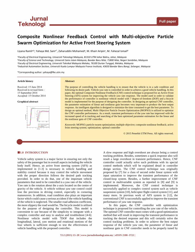
The purpose of controlling the vehicle handling is to ensure that the vehicle is in a safe condition and following its desire path. Vehicle yaw rate is controlled in order to achieve a good vehicle handling. In this
paper, the optimal Composite Nonlinear Feedback (CNF) control technique is proposed for an Active Front
Steering (AFS) system for improving the vehicle yaw rate response. The model used in order to validate the performance of controller is nonlinear vehicle model with 7 degree-of-freedom (DOF) and a bicycle
model is implemented for the purpose of designing the controller. In designing an optimal CNF controller,
the parameter estimation of linear and nonlinear gain becomes very important to produce the best output response. An intelligent algorithm is designed to minimize the time consumed to get the best parameter. To
design an optimal method, Multi Objective Particle Swarm Optimization (MOPSO) is utilized to optimize
the CNF controller performance. As a result, transient performance of the yaw rate has improved with the increased speed of in tracking and searching of the best optimized parameter estimation for the linear and
the nonlinear gain of CNF controller. Keywords: MOPSO; particle swarm optimization; multiple objective; composite nonlinear feedback; active front steering system; optimization; optimal controller
© 2015 Penerbit UTM Press. All rights reserved.
1.0 INTRODUCTION
Vehicle safety system is a major factor in ensuring not only the
safety of the passenger but in overall aspects including the vehicle
body itself. Hence, an active front steering system (AFS) as
implemented in [1-3] is necessary in vehicle handling and
stability control because it may control the vehicle movement
with the proper direction follows the desired path tracking
provided. In order to do that, one of the important vehicle
parameters that need to be controlled is a yaw rate of the vehicle.
Yaw rate is the rotation about the z-axis located on the centre of
gravity of the vehicle. A vehicle without yaw rate control could
lose the precision in driving control, especially in cornering
manoeuvres. In addition, road condition also plays an important
factor which could cause a serious accident if the vehicle handling
of the vehicle is neglected. The smaller road adhesion coefficient,
the more slippery the road would be. The bicycle model is utilized
for the purpose of designing the controller. This model is
convenient to use because of the simplicity to integrate with a
complex controller and easy to analyse and troubleshoot [4-6].
Nonlinear vehicle model with 7DOF that includes the
longitudinal, lateral, yaw motion and rotational motions of the
four wheels is sufficient enough to test the effectiveness of
vehicle handling with the proposed controller.
A slow response and high overshoot are always being a control
tracking problem. Besides, sometimes a quick response also will
result a large overshoot in transient performance. Hence, CNF
controller could actually solve such problems with its special
control methods which will be explained detail in controller
design section. The CNF control technique was originally
proposed by [7] for a class of second order linear system with
input saturation to improve the transient performance of the
closed-loop system. Besides, a further improvement of CNF
control in multivariable system as reported in [8] and [9] is
implemented. Moreover, the CNF control technique is
successfully applied to complex control system such as vehicle
suspension system [10], helicopter flight control system [11], and
many more. In previous work of AFS system in [12], the
conventional CNF is successfully applied to improve the transient
performance of yaw rate response.
In this paper, the CNF controller with optimization
technique is proposed for controlling the yaw rate of the vehicle.
The optimal CNF controller must comes with a good optimization
method that will result in improving the transient performance in
tracking the desired response and this will certainly solve the
control tracking problems. In order to achieve the best output
response of the vehicle yaw rate, the parameter of linear and
nonlinear gain in CNF controller needs to be properly tuned by
0 1 2 3 4 5 6 7 8-1
0
1
2
3
4
5
6
7
8
Time (s)
Yaw
rate
(d
eg
/s)
Optimal CNF by MOPSO
Without Controller
Reference
1.5 2 2.5
4
5
6
7
14 Yahaya Md. Sam et al. / Jurnal Teknologi (Sciences & Engineering) 72:2 (2015) 13–20
using a proper method. Based on [13], the authors have used some
performance criteria such as the Absolute-Value Of Error (IAE)
and the integral of time Multiplied Absolute-Error (ITAE).
Besides, Particle Swarm Optimization (PSO) [14], classical root
locus theory [8] and Hooke Jeeves method [15] are successfully
implemented. In our proposed controller, those parameters are
tuned simultaneously and precisely by solving the minimization
problems by using Multi Objective Particle Swarm Optimization
(MOPSO) which is the main objective of the paper. PSO is a part
of swarm intelligence family and well known in solving a very
large scale of nonlinear optimization problems.
Kennedy and Eberhart [16] were first established a solution
to the complex nonlinear optimization problem by imitating the
behavior of bird flocks. They generated the concept of function
optimization by means of a particle swarm. In fact, PSO has been
extended its ability and seems suitable to solve Multi Objective
Optimization Problem (MOOP) such as Multi Objective Particle
Swarm Optimization (MOPSO) [17-19]. Thus, MOPSO method
is proposed in this paper based on their effectiveness in tuning
parameters especially in meeting more than one objective target
[17, 20-22]. Those parameters in CNF control law are optimized
with three objective functions that are based on the transient
performance namely overshoot, settling time and steady state
error in finding the minimal error between the actual and the
desired response.
This paper is organized in 5 sections. Section 1 discussed an
overview of the previous work on the CNF controller design and
the effectiveness in using MOPSO to solve the optimization
problem. In Section 2, the methodology of the study is briefly
described comprises the vehicle model and reference model used
for the AFS system. Section 3 explains the design of the CNF
controller with MOPSO technique. The simulations results are
presented and analysed in Section 4 and ended with conclusion
and future work recommendation in Section 5.
2.0 VEHICLE DYNAMIC MODELS
There are two types of vehicle model used in this paper. Linear
single track vehicle model and nonlinear two track vehicle model
are discussed in this section. These two models are established
for designing the controller and as a vehicle plant respectively.
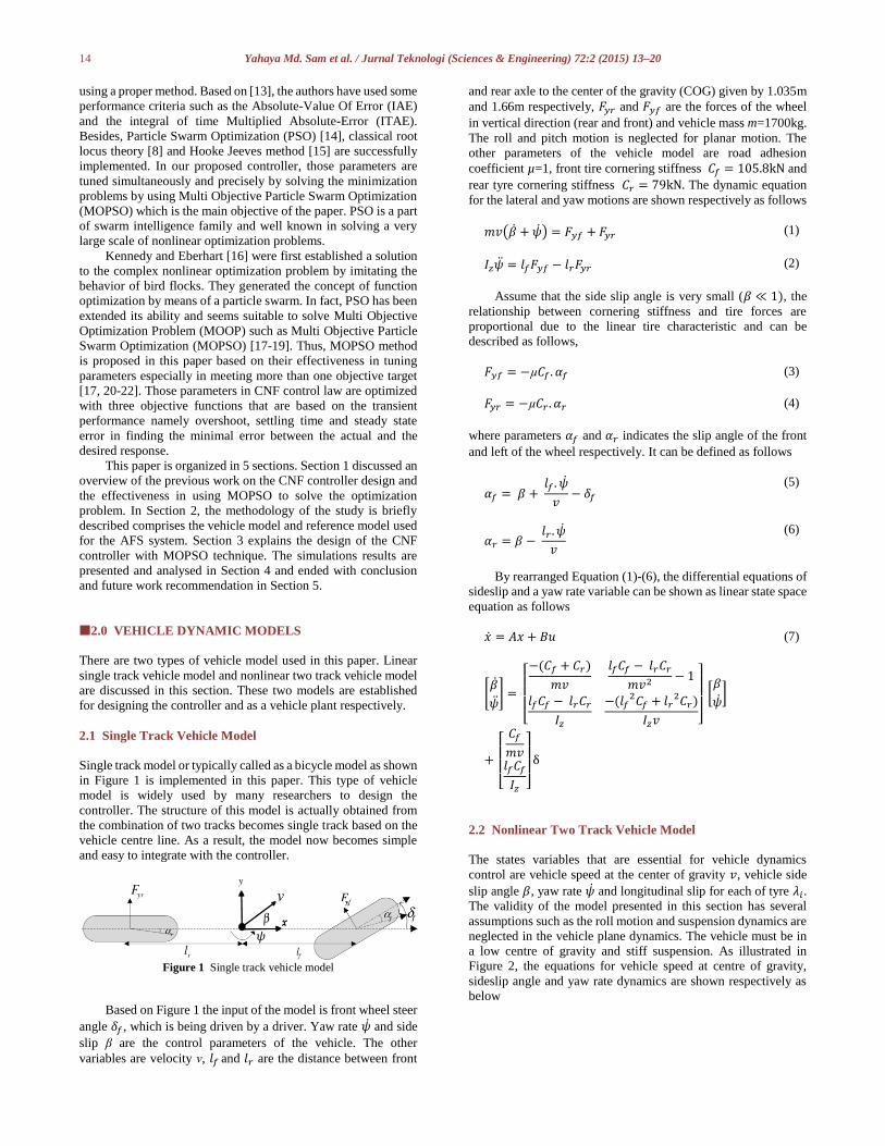
2.1 Single Track Vehicle Model
Single track model or typically called as a bicycle model as shown
in Figure 1 is implemented in this paper. This type of vehicle
model is widely used by many researchers to design the
controller. The structure of this model is actually obtained from
the combination of two tracks becomes single track based on the
vehicle centre line. As a result, the model now becomes simple
and easy to integrate with the controller.
Figure 1 Single track vehicle model
Based on Figure 1 the input of the model is front wheel steer
angle 𝛿𝑓, which is being driven by a driver. Yaw rate �̇� and side
slip β are the control parameters of the vehicle. The other
variables are velocity ν, 𝑙𝑓 and 𝑙𝑟 are the distance between front
and rear axle to the center of the gravity (COG) given by 1.035m
and 1.66m respectively, 𝐹𝑦𝑟 and 𝐹𝑦𝑓 are the forces of the wheel
in vertical direction (rear and front) and vehicle mass m=1700kg.
The roll and pitch motion is neglected for planar motion. The
other parameters of the vehicle model are road adhesion
coefficient µ=1, front tire cornering stiffness 𝐶𝑓 = 105.8kN and
rear tyre cornering stiffness 𝐶𝑟 = 79kN. The dynamic equation
for the lateral and yaw motions are shown respectively as follows
𝑚𝑣(�̇� + �̇�) = 𝐹𝑦𝑓 + 𝐹𝑦𝑟 (1)
𝐼𝑧�̈� = 𝑙𝑓𝐹𝑦𝑓 − 𝑙𝑟𝐹𝑦𝑟 (2)
Assume that the side slip angle is very small (𝛽 ≪ 1), the
relationship between cornering stiffness and tire forces are
proportional due to the linear tire characteristic and can be
described as follows,
𝐹𝑦𝑓 = −µ𝐶𝑓. 𝛼𝑓 (3)
𝐹𝑦𝑟 = −µ𝐶𝑟 . 𝛼𝑟 (4)
where parameters 𝛼𝑓 and 𝛼𝑟 indicates the slip angle of the front
and left of the wheel respectively. It can be defined as follows
𝛼𝑓 = 𝛽 + 𝑙𝑓 . �̇�
𝑣− 𝛿𝑓
(5)
𝛼𝑟 = 𝛽 − 𝑙𝑟 . �̇�
𝑣
(6)
By rearranged Equation (1)-(6), the differential equations of
sideslip and a yaw rate variable can be shown as linear state space
equation as follows
�̇� = 𝐴𝑥 + 𝐵𝑢
[�̇�
�̈�] =
[ −(𝐶𝑓 + 𝐶𝑟)
𝑚𝑣
𝑙𝑓𝐶𝑓 − 𝑙𝑟𝐶𝑟
𝑚𝑣2− 1
𝑙𝑓𝐶𝑓 − 𝑙𝑟𝐶𝑟
𝐼𝑧
−(𝑙𝑓2𝐶𝑓 + 𝑙𝑟
2𝐶𝑟)
𝐼𝑧𝑣 ]
[𝛽
�̇�]
+
[ 𝐶𝑓
𝑚𝑣𝑙𝑓𝐶𝑓
𝐼𝑧 ]
δ
(7)
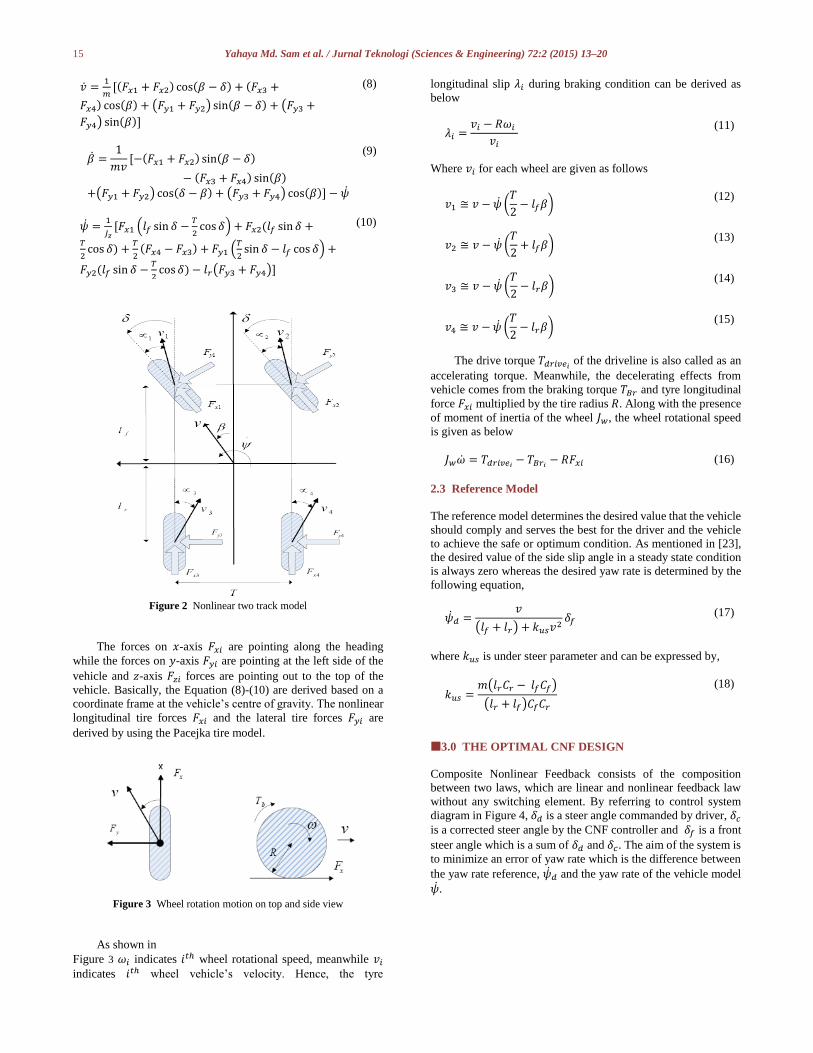
2.2 Nonlinear Two Track Vehicle Model
The states variables that are essential for vehicle dynamics
control are vehicle speed at the center of gravity 𝑣, vehicle side
slip angle 𝛽, yaw rate �̇� and longitudinal slip for each of tyre 𝜆𝑖. The validity of the model presented in this section has several
assumptions such as the roll motion and suspension dynamics are
neglected in the vehicle plane dynamics. The vehicle must be in
a low centre of gravity and stiff suspension. As illustrated in
Figure 2, the equations for vehicle speed at centre of gravity,
sideslip angle and yaw rate dynamics are shown respectively as
below
𝜓
15 Yahaya Md. Sam et al. / Jurnal Teknologi (Sciences & Engineering) 72:2 (2015) 13–20
�̇� =1
𝑚[(𝐹𝑥1 + 𝐹𝑥2) cos(𝛽 − 𝛿) + (𝐹𝑥3 +
𝐹𝑥4) cos(𝛽) + (𝐹𝑦1 + 𝐹𝑦2) sin(𝛽 − 𝛿) + (𝐹𝑦3 +
𝐹𝑦4) sin(𝛽)]
(8)
�̇� =1
𝑚𝑣[−(𝐹𝑥1 + 𝐹𝑥2) sin(𝛽 − 𝛿)
− (𝐹𝑥3 + 𝐹𝑥4) sin(𝛽)
+(𝐹𝑦1 + 𝐹𝑦2) cos(𝛿 − 𝛽) + (𝐹𝑦3 + 𝐹𝑦4) cos(𝛽)] − �̇�
(9)
�̇� =1
𝐽𝑧[𝐹𝑥1 (𝑙𝑓 sin 𝛿 −
𝑇
2cos 𝛿) + 𝐹𝑥2(𝑙𝑓 sin 𝛿 +
𝑇
2cos 𝛿) +
𝑇
2(𝐹𝑥4 − 𝐹𝑥3) + 𝐹𝑦1 (
𝑇
2sin 𝛿 − 𝑙𝑓 cos 𝛿) +
𝐹𝑦2(𝑙𝑓 sin 𝛿 −𝑇
2cos 𝛿) − 𝑙𝑟(𝐹𝑦3 + 𝐹𝑦4)]
(10)
Figure 2 Nonlinear two track model
The forces on 𝑥-axis 𝐹𝑥𝑖 are pointing along the heading
while the forces on 𝑦-axis 𝐹𝑦𝑖 are pointing at the left side of the
vehicle and 𝑧-axis 𝐹𝑧𝑖 forces are pointing out to the top of the
vehicle. Basically, the Equation (8)-(10) are derived based on a
coordinate frame at the vehicle’s centre of gravity. The nonlinear
longitudinal tire forces 𝐹𝑥𝑖 and the lateral tire forces 𝐹𝑦𝑖 are
derived by using the Pacejka tire model.
Figure 3 Wheel rotation motion on top and side view
As shown in
Figure 3 𝜔𝑖 indicates 𝑖𝑡ℎ wheel rotational speed, meanwhile 𝑣𝑖 indicates 𝑖𝑡ℎ wheel vehicle’s velocity. Hence, the tyre
longitudinal slip 𝜆𝑖 during braking condition can be derived as
below
𝜆𝑖 =𝑣𝑖 − 𝑅𝜔𝑖
𝑣𝑖
(11)
Where 𝑣𝑖 for each wheel are given as follows
𝑣1 ≅ 𝑣 − �̇� (𝑇
2− 𝑙𝑓𝛽)
(12)
𝑣2 ≅ 𝑣 − �̇� (𝑇
2+ 𝑙𝑓𝛽)
(13)
𝑣3 ≅ 𝑣 − �̇� (𝑇
2− 𝑙𝑟𝛽)
(14)
𝑣4 ≅ 𝑣 − �̇� (𝑇
2− 𝑙𝑟𝛽)
(15)
The drive torque 𝑇𝑑𝑟𝑖𝑣𝑒𝑖 of the driveline is also called as an
accelerating torque. Meanwhile, the decelerating effects from
vehicle comes from the braking torque 𝑇𝐵𝑟 and tyre longitudinal
force 𝐹𝑥𝑖 multiplied by the tire radius 𝑅. Along with the presence
of moment of inertia of the wheel 𝐽𝑤, the wheel rotational speed
is given as below
𝐽𝑤�̇� = 𝑇𝑑𝑟𝑖𝑣𝑒𝑖 − 𝑇𝐵𝑟𝑖 − 𝑅𝐹𝑥𝑖 (16)
2.3 Reference Model
The reference model determines the desired value that the vehicle
should comply and serves the best for the driver and the vehicle
to achieve the safe or optimum condition. As mentioned in [23],
the desired value of the side slip angle in a steady state condition
is always zero whereas the desired yaw rate is determined by the
following equation,
�̇�𝑑 =𝑣
(𝑙𝑓 + 𝑙𝑟) + 𝑘𝑢𝑠𝑣2𝛿𝑓 (17)
where 𝑘𝑢𝑠 is under steer parameter and can be expressed by,
𝑘𝑢𝑠 =𝑚(𝑙𝑟𝐶𝑟 − 𝑙𝑓𝐶𝑓)
(𝑙𝑟 + 𝑙𝑓)𝐶𝑓𝐶𝑟
(18)
3.0 THE OPTIMAL CNF DESIGN
Composite Nonlinear Feedback consists of the composition
between two laws, which are linear and nonlinear feedback law
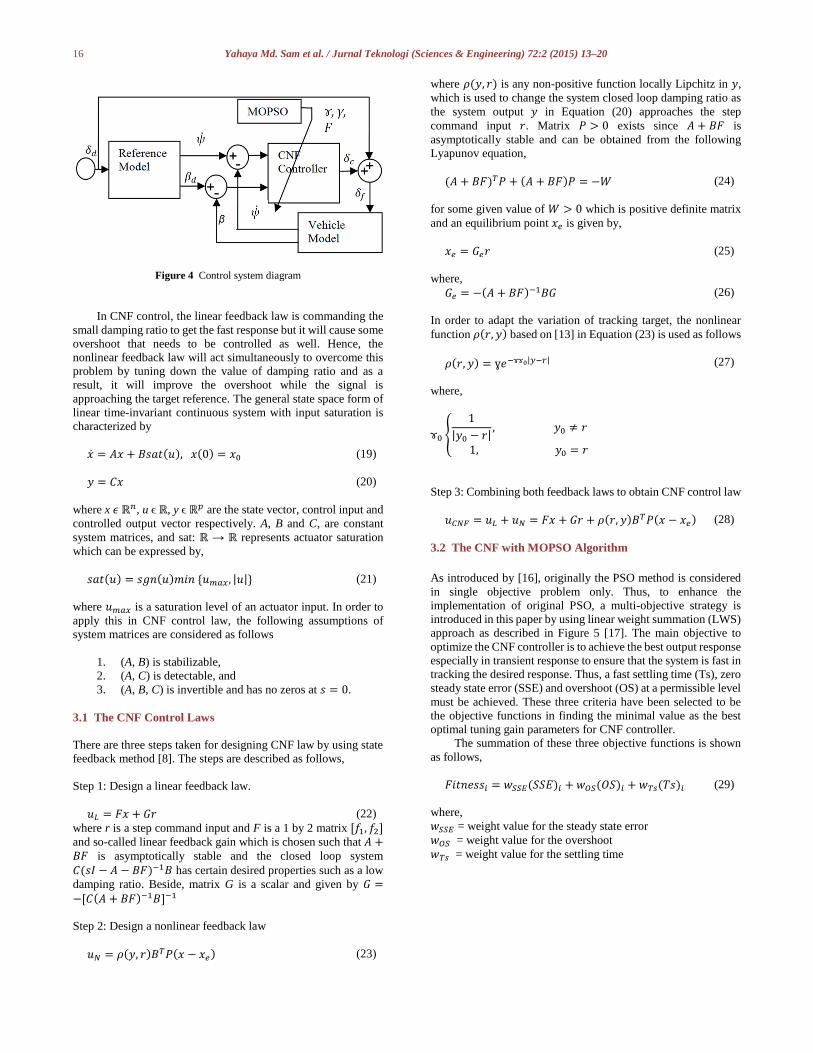
without any switching element. By referring to control system
diagram in Figure 4, 𝛿𝑑 is a steer angle commanded by driver, 𝛿𝑐 is a corrected steer angle by the CNF controller and 𝛿𝑓 is a front
steer angle which is a sum of 𝛿𝑑 and 𝛿𝑐. The aim of the system is
to minimize an error of yaw rate which is the difference between
the yaw rate reference, �̇�𝑑 and the yaw rate of the vehicle model
�̇�.
16 Yahaya Md. Sam et al. / Jurnal Teknologi (Sciences & Engineering) 72:2 (2015) 13–20
Figure 4 Control system diagram
In CNF control, the linear feedback law is commanding the
small damping ratio to get the fast response but it will cause some
overshoot that needs to be controlled as well. Hence, the
nonlinear feedback law will act simultaneously to overcome this
problem by tuning down the value of damping ratio and as a
result, it will improve the overshoot while the signal is
approaching the target reference. The general state space form of
linear time-invariant continuous system with input saturation is
characterized by
�̇� = 𝐴𝑥 + 𝐵𝑠𝑎𝑡(𝑢), 𝑥(0) = 𝑥0 (19)
𝑦 = 𝐶𝑥 (20)
where x 𝜖 ℝ𝑛, u ϵ ℝ, y ϵ ℝ𝑝 are the state vector, control input and
controlled output vector respectively. A, B and C, are constant
system matrices, and sat: ℝ → ℝ represents actuator saturation
which can be expressed by,
𝑠𝑎𝑡(𝑢) = 𝑠𝑔𝑛(𝑢)𝑚𝑖𝑛 {𝑢𝑚𝑎𝑥, |𝑢|} (21)
where 𝑢𝑚𝑎𝑥 is a saturation level of an actuator input. In order to
apply this in CNF control law, the following assumptions of
system matrices are considered as follows
1. (A, B) is stabilizable,
2. (A, C) is detectable, and
3. (A, B, C) is invertible and has no zeros at 𝑠 = 0.
3.1 The CNF Control Laws
There are three steps taken for designing CNF law by using state
feedback method [8]. The steps are described as follows,
Step 1: Design a linear feedback law.
𝑢𝐿 = 𝐹𝑥 + 𝐺𝑟 (22)
where r is a step command input and F is a 1 by 2 matrix [𝑓1, 𝑓2] and so-called linear feedback gain which is chosen such that 𝐴 +𝐵𝐹 is asymptotically stable and the closed loop system
𝐶(𝑠𝐼 − 𝐴 − 𝐵𝐹)−1𝐵 has certain desired properties such as a low
damping ratio. Beside, matrix G is a scalar and given by 𝐺 =−[𝐶(𝐴 + 𝐵𝐹)−1𝐵]−1
Step 2: Design a nonlinear feedback law
𝑢𝑁 = 𝜌(𝑦, 𝑟)𝐵𝑇𝑃(𝑥 − 𝑥𝑒) (23)
where 𝜌(𝑦, 𝑟) is any non-positive function locally Lipchitz in 𝑦,
which is used to change the system closed loop damping ratio as
the system output 𝑦 in Equation (20) approaches the step
command input 𝑟. Matrix 𝑃 > 0 exists since 𝐴 + 𝐵𝐹 is
asymptotically stable and can be obtained from the following
Lyapunov equation,
(𝐴 + 𝐵𝐹)𝑇𝑃 + (𝐴 + 𝐵𝐹)𝑃 = −𝑊 (24)
for some given value of 𝑊 > 0 which is positive definite matrix
and an equilibrium point 𝑥𝑒 is given by,
𝑥𝑒 = 𝐺𝑒𝑟 (25)
where,
𝐺𝑒 = −(𝐴 + 𝐵𝐹)−1𝐵𝐺 (26)
In order to adapt the variation of tracking target, the nonlinear
function 𝜌(𝑟, 𝑦) based on [13] in Equation (23) is used as follows
𝜌(𝑟, 𝑦) = ɣ𝑒−ɤɤ0|𝑦−𝑟| (27)
where,
ɤ0 {
1
|𝑦0 − 𝑟|, 𝑦0 ≠ 𝑟
1, 𝑦0 = 𝑟
Step 3: Combining both feedback laws to obtain CNF control law
𝑢𝐶𝑁𝐹 = 𝑢𝐿 + 𝑢𝑁 = 𝐹𝑥 + 𝐺𝑟 + 𝜌(𝑟, 𝑦)𝐵𝑇𝑃(𝑥 − 𝑥𝑒) (28)
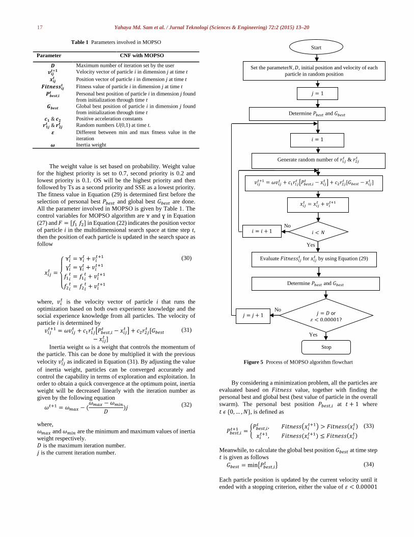
3.2 The CNF with MOPSO Algorithm
As introduced by [16], originally the PSO method is considered
in single objective problem only. Thus, to enhance the
implementation of original PSO, a multi-objective strategy is
introduced in this paper by using linear weight summation (LWS)
approach as described in Figure 5 [17]. The main objective to
optimize the CNF controller is to achieve the best output response
especially in transient response to ensure that the system is fast in
tracking the desired response. Thus, a fast settling time (Ts), zero
steady state error (SSE) and overshoot (OS) at a permissible level
must be achieved. These three criteria have been selected to be
the objective functions in finding the minimal value as the best
optimal tuning gain parameters for CNF controller.
The summation of these three objective functions is shown
as follows,
𝐹𝑖𝑡𝑛𝑒𝑠𝑠𝑖 = 𝑤𝑆𝑆𝐸(𝑆𝑆𝐸)𝑖 + 𝑤𝑂𝑆(𝑂𝑆)𝑖 + 𝑤𝑇𝑠(𝑇𝑠)𝑖 (29)
where,
𝑤𝑆𝑆𝐸 = weight value for the steady state error
𝑤𝑂𝑆 = weight value for the overshoot
𝑤𝑇𝑠 = weight value for the settling time
17 Yahaya Md. Sam et al. / Jurnal Teknologi (Sciences & Engineering) 72:2 (2015) 13–20
Table 1 Parameters involved in MOPSO
Parameter CNF with MOPSO
𝑫 Maximum number of iteration set by the user
𝒗𝒊𝒋𝒕+𝟏 Velocity vector of particle i in dimension j at time t
𝒙𝒊𝒋𝒕 Position vector of particle i in dimension j at time t
𝑭𝒊𝒕𝒏𝒆𝒔𝒔𝒊𝒋𝒕 Fitness value of particle i in dimension j at time t
𝑷𝒃𝒆𝒔𝒕,𝒊𝒕 Personal best position of particle i in dimension j found
from initialization through time t
𝑮𝒃𝒆𝒔𝒕 Global best position of particle i in dimension j found
from initialization through time t
𝒄𝟏 & 𝒄𝟐 Positive acceleration constants
𝒓𝟏𝒋𝒕 & 𝒓𝟐𝒋
𝒕 Random numbers U(0,1) at time t.
𝜺 Different between min and max fitness value in the
iteration
𝝎 Inertia weight
The weight value is set based on probability. Weight value
for the highest priority is set to 0.7, second priority is 0.2 and
lowest priority is 0.1. OS will be the highest priority and then
followed by Ts as a second priority and SSE as a lowest priority.
The fitness value in Equation (29) is determined first before the
selection of personal best 𝑃𝑏𝑒𝑠𝑡 and global best 𝐺𝑏𝑒𝑠𝑡 are done.
All the parameter involved in MOPSO is given by Table 1. The
control variables for MOPSO algorithm are ɤ and ɣ in Equation
(27) and 𝐹 = [𝑓1 𝑓2] in Equation (22) indicates the position vector
of particle i in the multidimensional search space at time step t,
then the position of each particle is updated in the search space as
follow
𝑥𝑖𝑗𝑡 =
{
ɤ𝑖𝑡 = ɤ𝑖
𝑡 + 𝑣𝑖𝑡+1
ɣ𝑖𝑡 = ɣ𝑖
𝑡 + 𝑣𝑖𝑡+1
𝑓1𝑖𝑡 = 𝑓1𝑖
𝑡 + 𝑣𝑖𝑡+1
𝑓2𝑖𝑡 = 𝑓2𝑖
𝑡 + 𝑣𝑖𝑡+1
(30)
where, 𝑣𝑖𝑡 is the velocity vector of particle i that runs the
optimization based on both own experience knowledge and the
social experience knowledge from all particles. The velocity of
particle i is determined by
𝑣𝑖𝑗𝑡+1 = 𝜔𝑣𝑖𝑗
𝑡 + 𝑐1𝑟1𝑗𝑡 [𝑃𝑏𝑒𝑠𝑡,𝑖
𝑡 − 𝑥𝑖𝑗𝑡 ] + 𝑐2𝑟2𝑗
𝑡 [𝐺𝑏𝑒𝑠𝑡− 𝑥𝑖𝑗
𝑡 ]
(31)
Inertia weight ω is a weight that controls the momentum of
the particle. This can be done by multiplied it with the previous
velocity 𝑣𝑖𝑗𝑡 as indicated in Equation (31). By adjusting the value
of inertia weight, particles can be converged accurately and
control the capability in terms of exploration and exploitation. In
order to obtain a quick convergence at the optimum point, inertia
weight will be decreased linearly with the iteration number as
given by the following equation
𝜔𝑡+1 = 𝜔𝑚𝑎𝑥 − (𝜔𝑚𝑎𝑥 − 𝜔𝑚𝑖𝑛
𝐷)𝑗 (32)
where,
𝜔𝑚𝑎𝑥 and 𝜔𝑚𝑖𝑛 are the minimum and maximum values of inertia
weight respectively.
𝐷 is the maximum iteration number.
𝑗 is the current iteration number.
Figure 5 Process of MOPSO algorithm flowchart
By considering a minimization problem, all the particles are
evaluated based on 𝐹𝑖𝑡𝑛𝑒𝑠𝑠 value, together with finding the
personal best and global best (best value of particle in the overall
swarm). The personal best position 𝑃𝑏𝑒𝑠𝑡,𝑖 at 𝑡 + 1 where
𝑡 𝜖 {0,… , 𝑁}, is defined as
𝑃𝑏𝑒𝑠𝑡,𝑖𝑡+1 = {
𝑃𝑏𝑒𝑠𝑡,𝑖𝑡 , 𝐹𝑖𝑡𝑛𝑒𝑠𝑠(𝑥𝑖
𝑡+1) > 𝐹𝑖𝑡𝑛𝑒𝑠𝑠(𝑥𝑖𝑡)
𝑥𝑖𝑡+1, 𝐹𝑖𝑡𝑛𝑒𝑠𝑠(𝑥𝑖
𝑡+1) ≤ 𝐹𝑖𝑡𝑛𝑒𝑠𝑠(𝑥𝑖𝑡)
(33)
Meanwhile, to calculate the global best position 𝐺𝑏𝑒𝑠𝑡 at time step
𝑡 is given as follows
𝐺𝑏𝑒𝑠𝑡 = min{𝑃𝑏𝑒𝑠𝑡,𝑖𝑡 } (34)
Each particle position is updated by the current velocity until it
ended with a stopping criterion, either the value of 휀 < 0.00001
Set the parameter𝑁,𝐷, initial position and velocity of each
particle in random position
Stop
Determine 𝑃𝑏𝑒𝑠𝑡 and 𝐺𝑏𝑒𝑠𝑡
Generate random number of 𝑟1𝑗𝑡 & 𝑟2𝑗
𝑡
𝑗 = 1
𝑖 = 1
𝑣𝑖𝑗𝑡+1 = 𝜔𝑣𝑖𝑗
𝑡 + 𝑐1𝑟1𝑗𝑡 [𝑃𝑏𝑒𝑠𝑡,𝑖
𝑡 − 𝑥𝑖𝑗𝑡 ] + 𝑐2𝑟2𝑗
𝑡 [𝐺𝑏𝑒𝑠𝑡 − 𝑥𝑖𝑗𝑡 ]
𝑥𝑖𝑗𝑡 = 𝑥𝑖𝑗
𝑡 + 𝑣𝑖𝑡+1
𝑖 < 𝑁 𝑖 = 𝑖 + 1
𝑗 = 𝐷 or 휀 < 0.00001?
𝑗 = 𝑗 + 1
Evaluate 𝐹𝑖𝑡𝑛𝑒𝑠𝑠𝑖𝑗𝑡 for 𝑥𝑖𝑗
𝑡 by using Equation (29)
Start
Determine 𝑃𝑏𝑒𝑠𝑡 and 𝐺𝑏𝑒𝑠𝑡
No
Yes
No
Yes
18 Yahaya Md. Sam et al. / Jurnal Teknologi (Sciences & Engineering) 72:2 (2015) 13–20
or MOPSO algorithm has reached the maximum iteration that is
set by user.
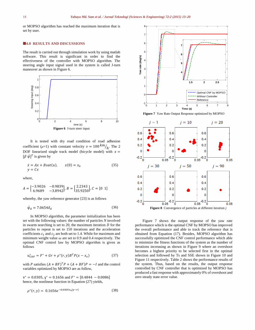
4.0 RESULTS AND DISCUSSIONS
The result is carried out through simulation work by using matlab
software. This result is significant in order to find the
effectiveness of the controller with MOPSO algorithm. The
steering angle input signal used in the system is called J-turn
maneuver as shown in Figure 6.
Figure 6 J-turn steer input
It is tested with dry road condition of road adhesion
coefficient (μ=1) with constant velocity 𝑣 = 100𝑘𝑚 ℎ⁄ . The 2
DOF linearized single track model (bicycle model) with 𝑥 =
[𝛽 �̇�]𝑇 is given by
�̇� = 𝐴𝑥 + 𝐵𝑠𝑎𝑡(𝑢), 𝑥(0) = 𝑥0
𝑦 = 𝐶𝑥
(35)
where,
𝐴 = [−3.9026 −0.98396.9689 −3.8942
], 𝐵 = [2.234335.9250
], 𝐶 = [0 1]
whereby, the yaw reference generator [23] is as follows
�̇�𝑑 = 7.0654𝛿𝑑 (36)
In MOPSO algorithm, the parameter initialization has been
set with the following values: the number of particles N involved
in swarm searching is set to 20, the maximum iteration 𝐷 for the
particles to repeat is set to 150 iterations and the acceleration
coefficients 𝑐1 and 𝑐2 are both set to 1.4. While for maximum and
minimum weight value 𝜔 are set to 0.9 and 0.4 respectively. The
optimal CNF control law by MOPSO algorithm is given as
follows
𝑢𝐶𝑁𝐹∗ = 𝐹∗ + 𝐺𝑟 + 𝜌∗(𝑟, 𝑦)𝐵𝑇𝑃(𝑥 − 𝑥𝑒) (37)
with 𝑃 satisfies (𝐴 + 𝐵𝐹)𝑇𝑃 + (𝐴 + 𝐵𝐹)𝑃 = −𝐼 and the control
variables optimized by MOPSO are as follow,
ɤ∗ = 0.0305, ɣ∗ = 0.1656 and 𝐹∗ = [0.4844 − 0.0086] hence, the nonlinear function in Equation (27) yields,
𝜌∗(𝑟, 𝑦) = 0.1656𝑒−0.0305ɤ0|𝑦−𝑟| (38)
Figure 7 Yaw Rate Output Response optimized by MOPSO
Figure 8 Convergence of particles at different iteration j
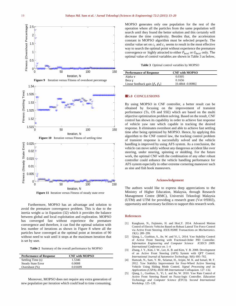
Figure 7 shows the output response of the yaw rate
performance which is the optimal CNF by MOPSO has improved
the overall performance and able to track the reference that is
obtained from Equation (17). Besides, MOPSO algorithm has
successfully optimized the CNF control performance which able
to minimize the fitness functions of the system as the number of
iterations increasing as shown in Figure 9 where an overshoot
becomes a highest priority to be selected first in the optimal
selection and followed by Ts and SSE shown in Figure 10 and
Figure 11 respectively. Table 2 shows the performance results of
the system. Thus, based on the results, the output response
controlled by CNF controller that is optimized by MOPSO has
produced a fast response with approximately 0% of overshoot and
zero steady state error value.
0 2 4 6 8 100
0.2
0.4
0.6
0.8
1
Ste
ering I
nput
(deg)
time (s)
0 1 2 3 4 5 6 7 8-1
0
1
2
3
4
5
6
7
8
Time (s)
Yaw
rate
(d
eg
/s)
Optimal CNF by MOPSO
Without Controller
Reference
1.5 2 2.5
4
5
6
7
19 Yahaya Md. Sam et al. / Jurnal Teknologi (Sciences & Engineering) 72:2 (2015) 13–20
Figure 9 Iteration versus Fitness of overshoot percentage
Figure 10 Iteration versus Fitness of settling time
Figure 11 Iteration versus Fitness of steady state error
Furthermore, MOPSO has an advantage and solution to
avoid the premature convergence problem. This is due to the
inertia weight 𝜔 in Equation (32) which it provides the balance
between global and local exploitation and exploration. MOPSO
has converged fast without experience the premature
convergence and therefore, it can find the optimal solution with
less number of iterations as shown in Figure 8 where all the
particles have converged at the optimal point at iteration of 90
without need to wait until it stops at the maximum iteration that
is set by user.
Table 2 Summary of the overall performance by MOPSO
Performance of Response CNF with MOPSO
Settling Time (s) 1.5346
Steady State Error 0.0008 Overshoot (%) 0.01699
Moreover, MOPSO does not require any extra generation of
new population per iteration which could lead to time consuming.
MOPSO generates only one population for the rest of the
operation where all the particles from the same population will
search until they found the better solution and this certainly will
decrease the time complexity. Besides that, the acceleration
constant in MOPSO algorithm must be selected properly. The
similar value set on 𝑐1 and 𝑐1 seems to result in the most effective
way to search the optimal point without experience the premature
convergence or highly attracted to either 𝑃𝑏𝑒𝑠𝑡 or 𝐺𝑏𝑒𝑠𝑡 only. The
optimal value of control variables are shown in Table 3 as below,
Table 3 Optimal control variables by MOPSO
Performance of Response CNF with MOPSO
Alpha ɤ 0.0305
Beta ɣ 0.1656
Linear feedback gain [𝒇𝟏 𝒇𝟐] [0.4844 -0.0086]
5.0 CONCLUSIONS
By using MOPSO in CNF controller, a better result can be
obtained by focusing on the improvement of transient
performance (Ts, OS and SSE) which are based on the multi
objective optimization problem solving. Based on the result, CNF
control has shown its capability in order to achieve fast response
of vehicle yaw rate which capable in tracking the desired
response. It eliminates overshoot and able to achieve fast settling
time after being optimized by MOPSO. Hence, by applying this
algorithm to the CNF control law, the tracking control problem
of transient response is successfully solved and the vehicle
handling is improved by using AFS system. As a conclusion, the
vehicle can move safely without any dangerous accident like over
steering, under steering, spinning or skidding. For the future
work, the optimal CNF with the combination of any other robust
controller could enhance the vehicle handling performance for
AFS system especially in other extreme cornering maneuver such
as sine and fish hook maneuvers.
Acknowledgement
The authors would like to express deep appreciations to the
Ministry of Higher Education, Malaysia, through Research
Management Centre (RMC), Universiti Teknologi Malaysia
(UTM) and UTM for providing a research grant (Vot 05H02),
opportunity and necessary facilities to support this research work.
References
[1] Kanghyun, N., Fujimoto, H. and Hori,Y. 2014. Advanced Motion
Control of Electric Vehicles Based on Robust Lateral Tire Force Control
via Active Front Steering. IEEE/ASME Transactions on Mechatronics.
19(1): 289–299.
[2] Qiang, L., Guobiao, S., Jie, W. and Yi, L. 2014. Yaw Stability Control
of Active Front Steering with Fractional-Order PID Controller. Information Engineering and Computer Science ICIECS 2009.
International Conference on. 1–4
[3] Zhang, J. Y., Kim, J. W., Lee, K. B. and Kim, Y. B. 2008. Development
of an Active Front Steering (AFS) System with QFT Control.
International Journal of Automotive Technology. 9(6): 695–702.
[4] Hamzah, N., Sam, Y. M., Selamat, H., Aripin, M. K. and Ismail, M. F.
2012. Yaw Stability Improvement for Four-Wheel Active Steering
Vehicle Using Sliding Mode Control. Signal Processing and its Applications (CSPA), IEEE 8th International Colloquium. 127–132.
[5] Qiang, L., Guobiao, S., Yi, L. and Jie, W. 2010. Yaw Rate Control of
Active Front Steering Based on Fuzzy-logic Controller. Education
Technology and Computer Science (ETCS). Second International
Workshop. 125–128.
0 50 100 1500
0.5
1
1.5
2
2.5
Iteration, N
Fitness (
Overs
hoot
Perc
enta
ge)
0 50 100 1501.515
1.52
1.525
1.53
1.535
1.54
Iteration, N
Fitness (
Sett
ling T
ime)
0 50 100 1500
0.005
0.01
0.015
0.02
0.025
Iteration, N
Fitness (
Ste
ady S
tate
Err
or)
20 Yahaya Md. Sam et al. / Jurnal Teknologi (Sciences & Engineering) 72:2 (2015) 13–20
[6] Wu, Y., Song, D., Hou, Z. and Yuan, X. 2007. A Fuzzy Control Method
to Improve Vehicle Yaw Stability Based on Integrated Yaw Moment
Control and Active Front Steering. In Mechatronics and Automation,
2007. ICMA 2007. International Conference. 1508–1512.
[7] Lin, Z., M. Pachter, and S. Banda. 1998. Toward Improvement of Tracking Performance Nonlinear Feedback for Linear Systems.
International Journal of Control. 70(1): 1–11.
[8] Chen, B. M., Lee, T. H., Kemao, P. and Venkataramanan, V. 2003.
Composite Nonlinear Feedback Control for Linear Systems with Input
Saturation: Theory and An Application. Automatic Control, IEEE
Transactions on. 48(3): 427–439.
[9] Lan, W., Chen, B. M. and He, Y. 2006. On Improvement of Transient Performance in Tracking Control for a Class of Nonlinear Systems with
Input Saturation. Systems & Control Letters. 55(2): 132–138.
[10] Ismail, M. F., Sam, Y. M., Peng, K., Aripin, M. K. and Hamzah, N. 2012.
A Control Performance of Linear Model and the Macpherson Model for
Active Suspension System Using Composite Nonlinear Feedback. In
Control System, Computing and Engineering (ICCSCE), 2012 IEEE
International Conference. 227–233.
[11] Guoyang, C. and P. Kemao. 2007. Robust Composite Nonlinear Feedback Control With Application to a Servo Positioning System.
Industrial Electronics, IEEE Transactions on. 54(2): 1132–1140.
[12] Aripin, M. K., Sam, Y. M., Kumeresan, A. D., Peng, K., Hasan, M. and
Ismail, M. F. 2013. A Yaw Rate Tracking Control of Active Front
Steering System Using Composite Nonlinear Feedback. In AsiaSim
2013. Springer Berlin Heidelberg. 231–242.
[13] Weiyao, L. and Chen, B. M. 2007. On Selection of Nonlinear Gain in
Composite Nonlinear Feedback Control for a Class Of Linear Systems. In Decision and Control, 2007 46th IEEE Conference. 1198–1203.
[14] Ramli, L., Sam, Y. M., Aripin, Z. Mohamed, M. K. Aripin and Ismail,
M. F. 2013. Optimal Composite Nonlinear Feedback Controller for an
Active Front Steering System. Applied Mechanics and Materials, 2014.
554: 526–530.
[15] Weiyao, L., Thum, C. K. and Chen, B.M. 2010. A Hard-Disk-Drive
Servo System Design Using Composite Nonlinear-Feedback Control
With Optimal Nonlinear Gain Tuning Methods. Industrial Electronics,
IEEE Transactions. 57(5): 1735–1745.
[16] Kennedy, J. and R. Eberhart. Particle Swarm Optimization. Neural Networks, 1995. Proceedings., IEEE International Conference. 1942–
1948.
[17] Jaafar, H. I., Sulaima, M. F., Mohamed, Z. and Jamian, J. J. 2013.
Optimal PID Controller Parameters for Nonlinear Gantry Crane System
via MOPSO Technique. Sustainable Utilization and Development in
Engineering and Technology (CSUDET), 2013 IEEE Conference. 86–
91. [18] Mahmoodabadi, M. J., Taherkhorsandi, M. and Bagheri, A. 2014.
Optimal Robust Sliding Mode Tracking Control of a Biped Robot Based
on Ingenious Multi-objective PSO. Neurocomputing. 124(0): 194–209.
[19] Domínguez, M., Fernández-Cardador, A., Cucala, A. P., Gonsalves, T.
and Fernández, A.. 2014. Multi Objective Particle Swarm Optimization
Algorithm for the Design of Efficient ATO Speed Profiles in Metro
Lines. Engineering Applications of Artificial Intelligence. 29: 43–53.
[20] Li, J. Z., L., Zeng, J. T, Xia, J. W.i, Li, M. H. and Liu, C. X. 2009. Research on Grid Workflow Scheduling Based on MOPSO Algorithm.
Intelligent Systems. GCIS '09. WRI Global Congress. 199–203.
[21] Kitamura, S., Mori, K., Shindo, S., Izui, Y. and Ozaki, Y. 2005.
Multiobjective Energy Management System Using Modified MOPSO.
Systems, Man and Cybernetics, 2005 IEEE International Conference.
3497–3503.
[22] Sharaf, A. M. and El-Gammal, A. A. A. 2009. A novel Discrete Multi-
Objective Particle Swarm Optimization (MOPSO) of Optimal Shunt Power Filter. Power Systems Conference and Exposition, 2009. PSCE
'09. IEEE/PES. 1–7.
[23] Mirzaei, M. 2010. A New Strategy for Minimum Usage of External Yaw
Moment in Vehicle Dynamic Control System. Transportation Research
Part C: Emerging Technologies. 18(2): 213–224.