851055

7/28/2019 851055

http://slidepdf.com/reader/full/851055 1/16

A production,distribution andinvestment model for a

multinational company Zubair M. Mohamed and

Mohamed A. Youssef

The authors

Zubair M. Mohamed is Professor, the Department of Management and Information Systems, Gordon Ford College of Business Administration, Western Kentucky University,Bowling Green, Kentucky, USA.Mohamed A. Youssef is Chair/Professor of Management,Department of Management and Decision Sciences, School of Business and Entrepreneurship, Norfolk State University, Norfolk,

Virginia, USA.

Keywords

Production planning, Distribution channels,Optimization techniques, Supply chain management

Abstract

Considerable research literature exists on production planning,distribution, and investment models. In most cases they havebeen treated independently in an environment of low inflationrates. Unfortunately, work extending these problems tomultinational companies is sparse. This paper develops anintegrated production planning, distribution, and investment

model for a multinational firm that produces products indifferent countries and distributes them to geographicallydiverse markets. Since multinational corporations operate indifferent countries under varying exchange and inflation rates,varying opportunities for investing, and differing regulations,these factors should be included in the decision process. In themodeling, the paper incorporates these factors and elicits theperformance of the model through an example and discusses theresults. The results indicate that the exchange rates and initialcapacity levels of the firms have significant effects on theproduction, distribution, and investment decisions, andconsequently, on the profit.

Electronic access

The Emerald Research Register for this journal isavailable atwww.emeraldinsight.com/researchregister

The current issue and full text archive of this journal isavailable atwww.emeraldinsight.com/1741-038X.htm

1. Introduction

A multinational corporation (MNC) is a firm that

engages in foreign direct investment and owns or

controls value-adding activities in more than one

country (Griffin and Pustay, 2002, p. 11). The

MNCs influence international trade. In 2000, the

total sales of world’s 500 largest corporations was$14.1 trillion ( Fortune, 2001, p. F1). Of these, 185

corporations or 37 percent are headquartered in

the USA, which underscores the importance of the

USA in the world economy. The international

trade in 1995 was about $5.5 trillion (Noori and

Radford, 1995) which grew to $7.8 trillion in 2000

(World Trade Organization, 2002). International

companies control about 25 percent of the $11

trillion global output, one-third of which is

produced in host countries (Schary and Skjott-

Larson, 2001). The revenues from abroad for US

companies are now twice their export earnings.

About one-fifth of the output of US firms is

produced overseas (Dornier et al., 1998, p. 76).

The multinational companies are growing more

rapidly as more and more companies are merging

(Wall Street Journal , 1998, p. A1), or being taken

over (Wall Street Journal , 1997, p. A1). Or, the

purchase of two youth-oriented Canadian apparel

chains by the American Eagle (Wall Street Journal ,

2000, p. B2).

However, managing international operations

presents a complex and challenging set of tasks.

Unfortunately, the research on the operational

modeling of MNCs is sparse. Hence, it is very

difficult to ascertain the effects of changes taking

place in one geographical location on the

functioning of the other facilities, and on the

overall performance of the MNCs. For example:. How do the fluctuations in foreign exchange

rates and inflation rates affect the functioning

of not only the host facility(ies) but also all

other facilities of the MNC?. What is the optimal way of financing the

operations?. Is it better to fund these operations with direct

money from the USA?. Is it better to borrow a proportion of budgeted

money from local sources?. Should they use some of the money earned

through prior investments in markets?. Are the return on the investments (seed

money) made are enough to sustain facilities

operations?

Journal of Manufacturing Technology Management

Volume 15 · Number 6 · 2004 · pp. 495-510

q Emerald Group Publishing Limited · ISSN 1741-038X

DOI 10.1108/17410380410547898

Received: January 2002

Revised: February 2003

Accepted: March 2003

The authors kindly acknowledge the contributions of

Andres Dingvall to the content of this paper.

495

7/28/2019 851055


. How do the changes in exchange rates and

inflation rates affect the logistics?. How do the changes in exchange rates and

inflation rates affect the strategic role of the

foreign facilities?

The integrated model developed in this paper can

address these and several other related questions.The model integrates production planning, product

distribution (logistics), and investment problems.

Production planning decisions involve determining,

for each facility, the products and their quantities to

be produced. In the ensuing process of production

planning, decisions regarding capacity, workforce

adjustments, overtime, subcontracting, and

machine capacity levels are also made for some

planning horizon, usually a one-year period.

Logistics decisions include which facilities

(suppliers) will cater to the demand of which

markets (distribution centers). Financial decisions

include investment opportunities, borrowing of

capital, disbursing of dividends and other related

decisions.

The impetus to develop an integrated model

was born out of the fact that such a model is

lacking in the current research literature. Mostly,

the above three problems have been treated

independently and perhaps is justifiable since

facilities and markets considered were operating

under low inflation rates. Recognizing that the

overall decisions for an MNC should consider all

facilities, markets and investment opportunities,

we attempt to fill the void by developing an

integrated production planning, distribution, and

financial investment model. Our model

incorporates the effects of varying inflation rates,

exchange rates, and other regulations under which

a facility has to operate in a host country(ies).

Exchange rates and inflation are two of the

complicating macroeconomic factors in the global

environment (Dornier et al., 1998, p. 224). Firms

such as Komatzu take advantage of fluctuations in

foreign currency to lower production costs by

moving production to the facilities in countries

whose currencies have depreciated (Heizer and

Render, 2000, p. 30). On the other hand, firms

find it difficult to operate under conditions of high

inflation rate as in the case of a Turkish firmreported in Kirca and Koksalan (1996).

The results from our model indicate that the

exchange rate and initial capacities of the facilities

have pronounced effects on profits, capacities

needed to satisfy demand, production and

distribution of products, and investments needed to

support facilities operations. Thus, we see the effects

of the exchange rate not only on the functioning of

the facility in a host country, but also on the

functioning of the domestic facility. The facilities’

first period operations are funded by direct funds

from the USA, and subsequent periods’ operations

are funded by the returns earned on the investments

made in the markets. As the return on the

investment is the main source of funding facilities’

operations, more money is invested in the markets of

facilities satisfying much of the global demand.

Where it is required to borrow money from local

sources, more money is borrowed when the dollar isstronger. When the dollar is weaker (low exchange

rates), the US facility satisfies much of the global

demand, and since it is assumed to be more

efficient, less capacity is consumed. Of course, more

profit is made and more money is invested in the

markets (since it is the main source of funding) as

compared to when the dollar is stronger. Many other

findings are discussed in Section 4.

The remainder of this paper is organized as

follows. In Section 2, we describe the growing

potential of global markets and the MNC

environment. In Section 3, we develop an integrated

production planning, distribution, and investmentmodel. In Section 4, we elicit the model’s

performance through numeric examples and discuss

results. In Section 5, we present and discuss our

conclusions.

2. MNC and its environment

Different terms abound for the MNC. They are:

global, world, transnational, international,

supernational, and supranational corporations

(Czinkota et al., 1994, p. 356). Likewise, there are

various definitions for an MNC. The United

Nations defines MNCs as “enterprises which own or

control production or service facilities outside the

country in which they are based”. Another definition

is “[MNC] is a firm that engages in foreign direct

investment and owns or controls value-adding

activities in more than one country” (Griffin and

Pustay, 2002, p. 11). Both definitions are economist

oriented (Rugman, 1981). They capture both the

quantitative and qualitative dimensions.

Quantitatively, for a firm to be regarded as

multinational, the number of countries of operation

is typically two, although the Harvard multinational

enterprise project required subsidiaries in six ormore nations (Vernon, 1971, p. 11). Another

measure is the proportion of overall revenues

generated from the foreign operations – 25 to 30

percent is the most often cited (Rugman, 1976). For

example, Caterpillar has 114 factories spread over

five continents and almost half of its revenues was

from overseas in 2001 (Griffin and Pustay, 2002,

p. 120) and McDonald has stores in 103 foreign

countries which contribute 59 percent of its total

operating income ( Fortune, 1997). The economic

power of the world’s largest entities is enormous.

A production, distribution and investment model

Zubair M. Mohamed and Mohamed A. Youssef


Volume 15 · Number 6 · 2004 · 495-510

496

7/28/2019 851055


Foreign direct investment (FDI) represents one

component of the international business flow and

includes start-ups of new operations, as well as

purchases of existing companies. The other

component is portfolio investment, which includes

the purchase of stocks and bonds internationally.

The growth of FDI is phenomenal. In 1967, it was

about $112 billion and in 1999 it was $3.5 trillion(World Bank, 1999). In 1994, the world’s ten

industrialized countries received half of the world’s

FDI and accounted for two-thirds of the world’s

accumulated stock of FDI (Ferdows, 1997). The

largest recipient was the USA and by 1994, foreign

multinationals had more than $500 billion in the

USA, up from $80 billion in 1980. FDI in the USA

totaled $1.2 trillion in 2000 with the UK being the

most important source of this FDI with $229.8

billion and, at the same time, US FDI abroad totaled

$1.2 trillion with the UK receiving $233.4 billion

(HighBeam Research, pp. 53, 90).

Qualitatively, for a firm to be an MNC, itsmanagement must consider it multinational and

must act accordingly. In terms of the management

philosophies, firms can be categorized as

ethnocentric (home-market oriented), polycentric

(oriented toward individual foreign market), and

regiocentric or geocentric (oriented toward larger

areas, even the global market place). We use the

term MNC in a global context – firms that view

their domestic operations as a part of worldwide

operations and direct an integrated business system.

Why do firms choose to be multinational? Firms

expand internationally for a variety of reasons.

According to Ferdows (1997), these reasonsinclude:. reduce direct and indirect costs;. reduce capital costs;. reduce taxes;. reduce logistics costs;. overcome tariff barriers;. provide better customer service;. spread foreign exchange risks;. build alternative supply sources;. preempt potential competitors;. learn from local suppliers, foreign customers,

foreign competitors, and foreign research

centers; and. attract talent globally.

These reasons can be broadly classified into

marketing factors, barriers to trade, cost factors,

investment climate, and general categories. Factors

considered in our model include cost of production

(manufacturing) and distribution (logistics), labor

costs (capacity), expertise in production and

distribution (efficiency), currency exchange

regulations, stability of foreign exchange,

opportunities in investing stocks and bonds, and

local debt.

There are six strategic roles for foreign factories of

MNCs (Ferdows, 1997, 2000). They are: off-shore

factory, source factory, server factory, contributor

factory, outpost factory, and lead factory.

An off-shore factory is established to produce

specific items at a low-cost and then export for

further rework or for sale. The primary purpose of a

source factory is also a low-cost production but giveslocal managers authority over production planning,

redesign, process changes, and out-bound logistics.

A source factory has the same ability to produce a

part as the best factory in the company’s global

network. A server factory supplies specific national

or regional markets. It typically provides a way to

overcome tariff barriers, logistics costs, and

exposure to foreign exchange fluctuations. A server

factory is not as developed or has powers as that of a

source facility. A contributor factory also serves a

national or regional market, as developed as a source

factory, and has more powers to develop products,

process engineering, sources of supply, anddevelopment of production capabilities. An outpost

factory’s primary role is to collect information. They

are located where competitors, research

laboratories, or customers are located. They also

serve the secondary strategic role as a server or an

off-shore, for example. A lead factory creates new

processes, products, and technologies for the entire

company. It should be noted that the choice of the

factory not only influences the location, but also the

operating decisions of the facility.

Managing global operations for a firm are more

difficult as it has to face different cultures, values,

rules, and varying degrees of business, political,and economical uncertainties. In other words,

globally operating companies are faced with far

more ambiguity, both internally and externally,

than their domestic counterparts. There are other

factors which further deter the global

competitiveness of a company. Shorter product life

cycles, fragmented and saturated markets, more

demanding customers, consolidation and mergers

of companies, and rapid advances in processes/

technology always present a dynamic competitive

situation. Hence, in this environment,

manufacturing and operations excellence are

critical factors for profitability, and globalization is

an essential component of the firm’s competitive

strategy. Globalization means moving production

facilities around to benefit from the quickest brains

or the cheapest labor to position a firm

competitively against its competition.

3. Model development

Initially, a firm has to decide whether it should

expand internationally. If it decides to become an




Volume 15 · Number 6 · 2004 · 495-510

497

7/28/2019 851055


MNC, then decisions related to international

location(s), production strategy (mode)/strategic

role, and operations have to be made.

Several studies have shown that transferring

production to foreign locations is a viable

alternative for lowering production costs, entry

into foreign markets, and avoiding import (export)

restrictions to gain competitive advantage indomestic and global markets. McDonald (1986)

claims that many manufacturing companies are

willing to locate their facilities in any part of the

world where they can obtain cheap labor, more

reliable materials, parts, subassemblies, vendors,

and governments that provide financial incentives.

However, Hoch (1982) points out that many US

firms fail to recognize the potential of these

investments – leading to faulty facility location.

The location decision is complex and involves

many factors (List and Catherine, 2000). Tong

and Walter (1980) using a questionnaire survey

conducted by mail, identified 32 possible locationvariables, and then using factor analysis narrowed

them down to five factors including availability of

transport services, labor attitudes, proximity of

markets, space for future expansion and suitable

plant sites. The attempt was to try and come up

with a handful of factors that could be considered

when foreign firms consider locations to setup

facilities. In another study Schemmer (1982) talks

about ten basic variables that firms looked at

before deciding on locations. They include labor,

climate, access to suppliers, and transportation to

name a few. We would like to note that these

factors continue to be relevant as reported recentlyby Karakaya and Canel (1998). The location

factors that are relevant to the model developed in

this paper include transportation costs, production

costs, and labor efficiency.

Various modeling techniques ranging from

capital budgeting, break-even analysis to fuzzy set

theory have been used in location decisions.

Mathematical modeling (network flow models) is

the most common approach used. Although

considerable modeling research exists pertaining

to the facilities location in domestic markets, work

regarding international facilities location is

limited. One of the first models of an internationalplant location was developed by Hodder and

Jucker (1982) and was later followed by few. The

recent work includes Canel and Khumawala

(1993, 1996), Min and Melachrinoudis (1996),

Flipo (2000), Syam (2000) and Verter (2002).

Production-related strategy could be direct

import, joint venture, and a wholly-owned

subsidiary. Kouvelis and Sinha (1994, 1995)

develop a stochastic dynamic programming model

that considers exchange rate, demand and pricing.

For each of the production strategies they develop

optimal solutions and also investigate the

conditions in which each strategy dominates the

others. A switching between production strategies

involves switching cost, however, the time required

to implement the change is assumed to be

insignificant. Axarloglou et al. (1995) presented an

empirical study to test the analytical results of

Kouvelis and Sinha’s model. They used data from

the Bureau of Economic Analysis, US Department

of Commerce. Kogut and Kulatilaka (1994) were

probably the first to develop a stochastic dynamic

programming model to this production switching

flexibility. In addition, Dasu and Li (1994) and

Huchzermeier and Cohen (1996) have looked into

this problem as well. These models are referred as

option valuation models. Option valuation models

are usually formulated as stochastic dynamic

programming models that seek to minimize

(maximize) expected costs (profits) over a finite or

infinite horizon. These models help utilize

operational flexibility which is available in terms of excess capacity. By holding excess capacity in

different plants, a firm can switch production

among these plants to avail opportunities

presented by exchange rates or counter problems

related to labor, supplies, etc.

The production planning and distribution

problem considered in this research is the supply

chain coordination problem. Coordination of

supply chain activities is a key concept for the global

firm (Cohen and Mallik, 1997). Network flow

models provide an effective approach for modeling

these supply chain coordination problems. Kogut

(1984, 1985a, b) was one of the first to describequalitatively the advantages of coordination of

global activities and strategies that capitalize on the

comparative advantages of countries and distributed

competence of international firms. However,

analytical modeling in this field is relatively new

(Cohen and Mallik, 1997). Recent literature surveys

on this topic can be found in the work of Verter and

Dincer (1992, 1995), Cohen and Kleindorfer

(1993), Vidal and Goetschalckx (1997) and Cohen

and Mallik (1997).

Cohen et al. (1989) develop a nonlinear mixed

integer programming model that lends itself to

hierarchical solution process and iterative process.The model considers exchange rates, tariffs, taxes,

sourcing, and taxes and maximizes profit. It assumes

that sufficient capacity exists to meet each period’s

demand without using inventories. Dasu and Torre

(1993a, b) develop a game-theoretic model to study

the coordination among the three affiliates of a US

MNC located in three Latin American countries.

They conclude that a policy of collaboration, under

almost all circumstances involving varying exchange

rates, tariffs, inflation rates, increase group

performance. In order to understand how a firm




Volume 15 · Number 6 · 2004 · 495-510

498

7/28/2019 851055


should use extra capacity to handle uncertainties in a

global environment, Rosenfield (1996) proposed a

series of formulations. His model determines the

number of plants and production levels at each

plant. The objective was to minimize the costs of

production and distribution to geographically

dispersed markets. The principal conclusions are

that it is better to have excess capacities in multipleplants and that the costs are minimized by building

plants of equal sizes.

Our model also pertains to the operations of an

MNC. The model developed in this paper is a

network flow optimization model. The question

we address is: “What are the production,

distribution, and investment decisions for an

MNC over a finite planning horizon?” That is,

which products will be made where, which

facilities would cater to which markets, and how

the funds will be obtained? The primary objective

an MNC is to maximize its profits. In addition to

addressing the questions raised in the Section 1,the model can address few other practical

questions. For example, the model can help

identify facilities requiring capacity additions and

when. Is it better to expand capacity when the

dollar is stronger or weaker? Is it better to dispose

idle capacity or retain capacity for future use?

What is the opportunity cost of meeting local

regulations or marketing needs even though the

facility in that market is not cost-effective?

Notations

The notations used in developing our model are

given in Table I.

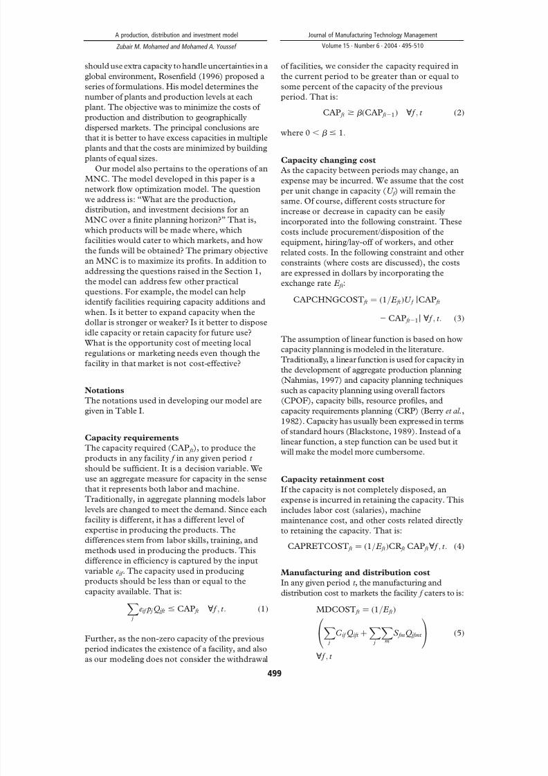
Capacity requirements

The capacity required (CAP ft ), to produce the

products in any facility f in any given period t

should be sufficient. It is a decision variable. We

use an aggregate measure for capacity in the sense

that it represents both labor and machine.

Traditionally, in aggregate planning models labor

levels are changed to meet the demand. Since each

facility is different, it has a different level of

expertise in producing the products. The

differences stem from labor skills, training, andmethods used in producing the products. This

difference in efficiency is captured by the input

variable e jf . The capacity used in producing

products should be less than or equal to the

capacity available. That is:

j

Xeif p j Q jft # CAP ft ; f ; t : ð1Þ

Further, as the non-zero capacity of the previous

period indicates the existence of a facility, and also

as our modeling does not consider the withdrawal

of facilities, we consider the capacity required in

the current period to be greater than or equal to

some percent of the capacity of the previous

period. That is:

CAP ft $ b ðCAP ft 21Þ ; f ; t ð2Þ

where 0,

b #

1:

Capacity changing cost

As the capacity between periods may change, an

expense may be incurred. We assume that the cost

per unit change in capacity (U f ) will remain the

same. Of course, different costs structure for

increase or decrease in capacity can be easily

incorporated into the following constraint. These

costs include procurement/disposition of the

equipment, hiring/lay-off of workers, and other

related costs. In the following constraint and other

constraints (where costs are discussed), the costs

are expressed in dollars by incorporating theexchange rate E ft :

CAPCHNGCOST ft ¼ ð1=E ft ÞU f jCAP ft

2CAP ft 21j ; f ; t : ð3Þ

The assumption of linear function is based on how

capacity planning is modeled in the literature.

Traditionally, a linear function is used for capacity in

the development of aggregate production planning

(Nahmias, 1997) and capacity planning techniques

such as capacity planning using overall factors

(CPOF), capacity bills, resource profiles, and

capacity requirements planning (CRP) (Berry et al.,1982). Capacity has usually been expressed in terms

of standard hours (Blackstone, 1989). Instead of a

linear function, a step function can be used but it

will make the model more cumbersome.

Capacity retainment cost

If the capacity is not completely disposed, an

expense is incurred in retaining the capacity. This

includes labor cost (salaries), machine

maintenance cost, and other costs related directly

to retaining the capacity. That is:

CAPRETCOST ft ¼ ð1=E ft ÞCR ft CAP ft ; f ; t : ð4Þ

Manufacturing and distribution cost

In any given period t , the manufacturing and

distribution cost to markets the facility f caters to is:

MDCOST ft ¼ ð1=E ft Þ

j

XC if Qift þ

j

Xm

XS fmQ jfmt

0@

1A

; f ; t

ð5Þ




Volume 15 · Number 6 · 2004 · 495-510

499

7/28/2019 851055


where the terms under first summation sign (C jf Q jft )

represent manufacturing costs and terms under the

second summation sign (S fm Q jfmt ) represent

distribution costs. We assume that the distribution

cost will be borne by facility f .

Demand satisfaction

In any given period t , the demand for product j in

each market m (D jmt ) has to be satisfied from someor all facilities. That is:

D jmt ¼ f

XQ jfmt ; j ; m; t : ð6Þ

Inventory cost

It is possible for a firm to produce more units of a

product in one period and hold it in inventory (I jft )

to satisfy the demand of the future period(s). The

inventory held and the inventory cost incurred are:

I jft 21 þ Q jft ¼m

XQ jfmt þ I jft ; j ; f ; t ð7Þ

IHCOST ft ¼ ð1=E ft Þ j

Xh jft I jft ; f ; t : ð8Þ

Exchange rate function

Exchange rate is a random variable. The difficulty

economists have had in finding an empirically

successful exchange rate theory is well

documented (Harvey, 1996; Taylor, 1995a, b).

Nonetheless, a firm has to forecast what the rate

would be in the future in order to make the

appropriate decisions. We will use the following

linear function for the exchange rate:

E ft ¼ ð1 þ a f t ÞE f ; f ð9Þ

Table I

Notation Explanation

Input variables

J Set of products {1,2,. . ., j ,. . .J}

F Set of facilities {1,2,. . .f ,. . .F}

M Set of markets {1,2,. . .,m ,. . .M}

T Set of time periods {1,2,. . .

,t ,. . .

,T}D jmt Demand for product j in period t for market m

R jm Revenue/unit of product j in market m

C jf Manufacturing cost/unit of product j in facility f

CRft Unit capacity retaining cost of facility f in period t

S fm Unit shipping cost from facility f to market m

h jft Unit inventory holding cost of product j in facility f in period t

U f Unit capacity changing cost in facility f

b Minimum capacity level retainment

E ft Exchange rate of currency of host country in period t

p j Unit processing time of product j in the USA

e jf Efficiency of facility f in producing product j compared with the USA

w f Minimum percent of budget of facility f to be borrowed from the local sources

r ift Interest rate earned on the investments in markets of facility f in period t

r bft Interest rate paid on the funds borrowed in period t from the markets of facility f OTHERCOSTft Other costs incurred in the facility f in period t

Decision variables

CAPft Capacity of facility f in period t

CAPCHNGCOSTft Capacity changing cost of facility f in period t

CAPRETCOSTft Capacity retaining cost of facility f in period t

MDCOSTft Manufacturing and distributing cost of facility f in period t

Q jft Quantity of product j produced in facility f in period t

Q jfmt Quantity of product j shipped from facility f to market m in period t

I jft Ending inventory of product j in facility f in period t

IHCOSTft Inventory holding cost of facility of f in period t

BUDft Budget requirements of facility f in period t

MFUNDus-ft Funds for manufacturing from the USA to facility f in period t

INVft Funds invested in period t in the markets where facility f is located

MINVft Funds withdrawn from the markets of facility f in period t BORft Funds borrowed from the markets of facility f

PROFITt Total profit in period t




Volume 15 · Number 6 · 2004 · 495-510

500

7/28/2019 851055


where E f is the base exchange rate and a f is the

forecast coefficient for the exchange rate. Sensitivity

analysis with respect to this value will test the

robustness of the solution. A similar linear model has

been developed by Harvey and Quinn (1997). Their

empirical model is based on the premise that the

exchange rates are a function of expectations. They

used regression analysis on the data obtained fromexpectations surveys published by Money Market

Services International and noon buying rates in New

York city reported by the Federal Reserve Bank of

New York. Their linear model has a constant term

and a second term that reflects the change in the

foreign currency price of the dollar from one period

of time to another (i.e. a time function).

Budget requirements

The budget (BUD ft ) required to sustain operations

for any period should be sufficient. This can come

directly as manufacturing funds from US

(MFUNDus- ft ), borrowing from local markets

(BOR ft ), and prior investment made in the local

markets (MINV ft 21). We confine ourselves to

investment in only those markets where facilities

are located, however, investment in other markets

can be easily incorporated. The budget should take

care of the costs incurred due to manufacturing

and distribution, other costs, capacity changing

costs, capacity retaining costs, and inventory

holding costs in each period for each facility. The

following constraints capture the budgetary

requirements. The OTHERCOST ft category

includes administrative expenses and

miscellaneous expenses:

BUD ft ¼ MDCOST ft

þ ð1=E ft ÞOTHERCOST ft

þ CAPCHNGCOST ft

þ CAPRETCOST ft

þ IHCOST ft ; f ; t ð10Þ

BUD ft ¼ MFUNDus- ft þ ð1=E ft ÞBOR ft

þ MINV ft 21 ; f ; t : ð11Þ

In constraint (11), we assume that money can be

invested for one period and there is no penalty for

early withdrawal. This is considered as in the long

run, a firm may choose to take out money from the

investment rather than transfer funds from the

USA.

Also, firms have to operate under some foreign

government regulations. For example, some part

of the funds required for the budget have to be

borrowed from the local sources to stimulate the

local economy or curb inflation. We consider the

local source as banks and not issuing of stocks or

bonds. The reason is the issuing of bonds or stocks

would involve disbursing dividends and this would

make the model more cumbersome:

ð1=E ft ÞBOR ft ’w f BUD ft ; f ; t ð12Þ

where w f is the percent of budget that has to be

borrowed.

Investment income from foreign country

As stated before, a firm has the option of investing

(INV ft ) in the market of host countries where

facilities are located. We do not consider the

investment opportunities in other countries to

keep the model simple. A part (MINV ft 21) of the

prior period’s investment (INV ft 21) can be

withdrawn to finance the operations of the current

period and the rest can be reinvested. Also, there is

an opportunity to invest funds from the USA in the

current period (INVus- ft ). We do not consider

separately the ploughing back of profits made from

the facility of the host country towards its

operations since the same money can come to the

USA and be fed back to the host country as funds

from the USA.

INV ft ¼ INVus- ft þ ð1 þ r ift ÞINV ft 21

2MINV ft 21 ; f ; t : ð13Þ

Constraint (13) implies that the total investment

(INV ft ) in the market of a host country should

equal the sum of direct investment made (INVus-

ft ), the principal and return earned on a previous

investment ðð1 þ r ift ÞINV ft 21Þ; minus the amount

withdrawn (MINV ft 21) to sustain manufacturing

operations.

Profit from operations

In any period t , the factors affecting the profits

include profit from the sale of the products,

facilities’ operating costs, yields from the

investments, and payback of the borrowed capitalalong with interest. The products are sold in

different markets at different unit selling prices.

Since the manufacturing and distribution costs are

different as the products come from separate

facilities, the unit profits will be dissimilar. Also,

the yield from the funds invested in the local

markets in the previous period contributes to the

overall profits. Further, the profit equation should

consider the amount that has been borrowed from

the local sources and have to be repaid along with

interest. That is:




Volume 15 · Number 6 · 2004 · 495-510

501

7/28/2019 851055


PROFITt ¼ j

Xm

Xð1=E mt ÞR jmQ jm

2

f

X{MDCOST ft

þ CAPCHNGCOST ft

þ CAPRETCOST ft


þ IHCOST ft }

þ f

Xr ift 21INV ft 21

2

f

Xð1=E ft Þð1

þ r bft 21ÞBOR ft 21 ;t : ð14Þ

We have assumed that the funds borrowed from a

local market have to be paid by the next period. Of

course, this assumption can be easily changed to

incorporate the payment of debt at a later period.

Objective function

To compute revenues and costs, we consider the

prevailing exchange rates and interest rates, the

objective function can be modeled as the

maximization of future worth of profits. In the

following representation of the objective function,

the investment in the period prior to the last period

is subtracted since we do not want enormous

amounts to be invested in the prior period. This

would make the problem unbounded. Of course,

the inclusion of the last term should not alter the

production and distribution activities:

Maximizet

XPROFITt 2

f

XINV ft 21:

The complete integrated production, distribution,

and investment model (PDI) is:

Maximizet

XPROFITt 2

f

XINV ft 21

s.t.,

j

Xeif p j Q jft #CAP ft ; f ; t ð1Þ

CAP ft ’b CAP ft 21 ; f ; t ð2Þ

CAPCHNGCOST ft ¼ ð1=E ft ÞU f *CAP ft

2CAP ft 21* ; f ; t ð3Þ

CAPRETCOST ft ¼ ð1=E ft ÞCR ft CAP ft ; f ; t ð4Þ

MDCOST ft ¼ ð1=E ft Þ

j XC

jf Q

jft þ

j X

mXS

fmQ

jfmt

0@

1A

; f ; t

ð5Þ

D jmt ¼ f

XQ jfmt ; j ; m; t ð6Þ

I jft 21 þ Q jft ¼m

XQ jfmt þ I jft ; j ; f ; t ð7Þ

IHCOST ft ¼ ð1=E ft Þ j

Xh jft I jft ; f ; t ð8Þ

E ft ¼ ð1 þ a f t ÞE f ; f ð9Þ

BUD ft ¼ MDCOST ft


þ CAPCHNGCOST ft

þ CAPRETCOST ft

þ IHCOST ft ; f ; t ð10Þ

BUD ft ¼ MFUNDus- ft þ ð1=E ft ÞBOR ft

þ MINV ft 21 ; f ; t ð11Þ

ð1=E ft ÞBOR ft ’w f BUD ft ; f ; t ð12Þ

INV ft ¼ INVus- ft þ ð1 þ r ift ÞINV ft 21

2MINV ft 21 ; f ; t ð13Þ




Volume 15 · Number 6 · 2004 · 495-510

502

7/28/2019 851055


7/28/2019 851055


Before discussing the effects of exchange rates and

initial capacity levels, we will first list the following

observations common to all four cases:. Direct funds for manufacturing are made only

once in both facilities (countries).. Besides the initial investment that was there in

the markets of both countries, another

investment is made in the first period in bothcountries.

. Funds to sustain operations (budget) in both

countries come from the investments made in

the markets. Only in the case of the USA the

initial investment is consumed to sustain

operations, whereas, the initial investment

made in India continues to be in the market.. Much of the direct manufacturing funds made

in both facilities in the first period goes intoacquiring the capacity.

Table III Results for zero initial capacities and increasing exchange rates

Category Country Period 0 Period 1 Period 2 Period 3

Budget USA $434,131 $161,304 $150,266

INDIA $1,095,641 $394,876 $410,843

Investment USA $200,000 $308,485 $150,266 $1,503

INDIA $300,000 $608,090 $328,675 $23,007

Borrow USA

INDIA Rs6,847,757 Rs2,632,504 Rs2,833,403

Direct manufacturing funds USA $234,100

INDIA $876,513

Funds from investments USA $200,000 $161,304 $150,266 $1,503INDIA $315,900 $325,388

Direct investments in markets USA $306,485

INDIA $293,090

Production quantity distribution USA Ga I USA G I USA G

USA 9.04b 8.92 8

INDIA 0.96 14 20 3.08 8 25 14

Capacity USA 0 2,713h $271,331c 2,713h $0 2,713h $0

INDIA 0 20,973h $671,148 20,973h $0 20,973h $0

Profits 0 $1,134,698 $904,707

Notes: a G ¼ Germany, and I ¼ India; b Quantities in ’000s; c Capacity changing cost in that period; an inventory of 2,055 units were carried in India in the secondperiod

Figure 1 Representation of production, distribution, and investment model for a multinational company




Volume 15 · Number 6 · 2004 · 495-510

504

7/28/2019 851055


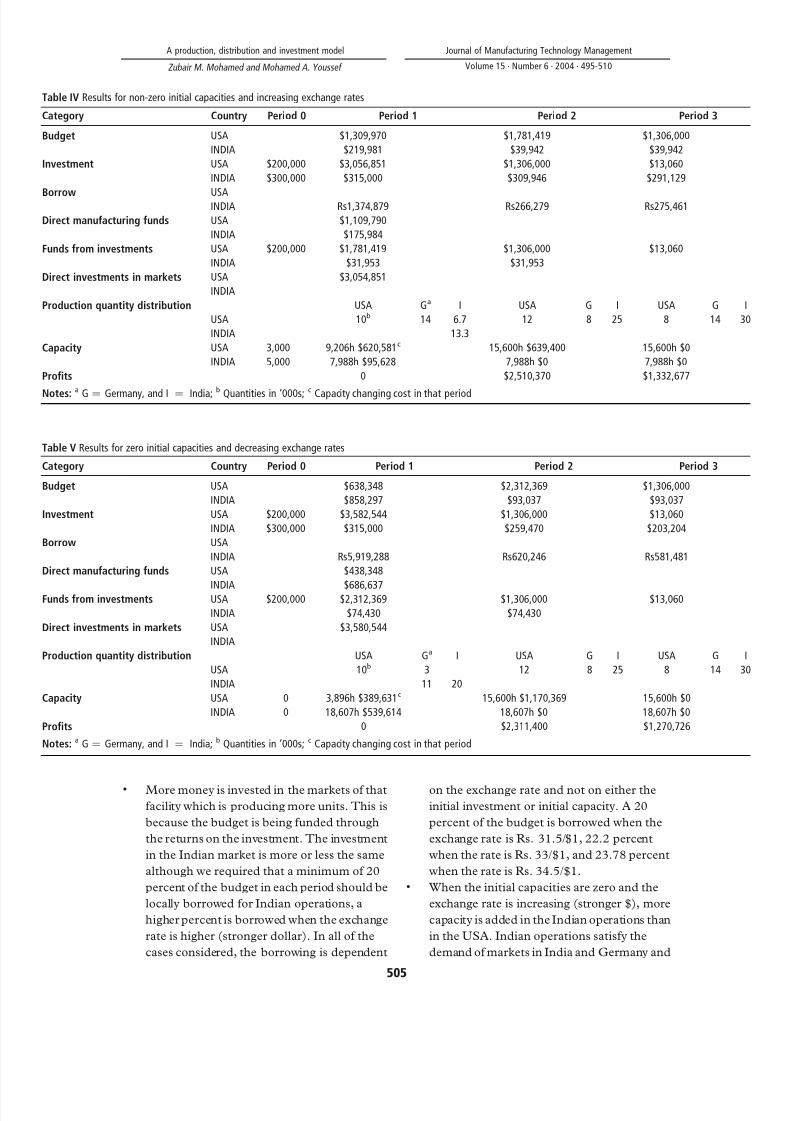
. More money is invested in the markets of that

facility which is producing more units. This is

because the budget is being funded through

the returns on the investment. The investment

in the Indian market is more or less the same

although we required that a minimum of 20

percent of the budget in each period should be

locally borrowed for Indian operations, a

higher percent is borrowed when the exchange

rate is higher (stronger dollar). In all of the

cases considered, the borrowing is dependent

on the exchange rate and not on either the

initial investment or initial capacity. A 20

percent of the budget is borrowed when the

exchange rate is Rs. 31.5/$1, 22.2 percent

when the rate is Rs. 33/$1, and 23.78 percent

when the rate is Rs. 34.5/$1.. When the initial capacities are zero and the

exchange rate is increasing (stronger $), more

capacity is added in the Indian operations than

in the USA. Indian operations satisfy the

demand of markets in India and Germany and

Table IV Results for non-zero initial capacities and increasing exchange rates


Budget USA $1,309,970 $1,781,419 $1,306,000

INDIA $219,981 $39,942 $39,942

Investment USA $200,000 $3,056,851 $1,306,000 $13,060

INDIA $300,000 $315,000 $309,946 $291,129

Borrow USAINDIA Rs1,374,879 Rs266,279 Rs275,461

Direct manufacturing funds USA $1,109,790

INDIA $175,984

Funds from investments USA $200,000 $1,781,419 $1,306,000 $13,060

INDIA $31,953 $31,953

Direct investments in markets USA $3,054,851

INDIA


USA 10b 14 6.7 12 8 25 8 14

INDIA 13.3

Capacity USA 3,000 9,206h $620,581c 15,600h $639,400 15,600h $0

INDIA 5,000 7,988h $95,628 7,988h $0 7,988h $0

Profits 0 $2,510,370 $1,332,677

Notes:a

G ¼ Germany, and I ¼ India;b

Quantities in ’000s;c

Capacity changing cost in that period

Table V Results for zero initial capacities and decreasing exchange rates


Budget USA $638,348 $2,312,369 $1,306,000

INDIA $858,297 $93,037 $93,037

Investment USA $200,000 $3,582,544 $1,306,000 $13,060

INDIA $300,000 $315,000 $259,470 $203,204

Borrow USA

INDIA Rs5,919,288 Rs620,246 Rs581,481


INDIA $686,637Funds from investments USA $200,000 $2,312,369 $1,306,000 $13,060

INDIA $74,430 $74,430


INDIA


USA 10b 3 12 8 25 8 14

INDIA 11 20

Capacity USA 0 3,896h $389,631c 15,600h $1,170,369 15,600h $0

INDIA 0 18,607h $539,614 18,607h $0 18,607h $0

Profits 0 $2,311,400 $1,270,726

Notes: a G ¼ Germany, and I ¼ India; b Quantities in ’000s; c Capacity changing cost in that period




Volume 15 · Number 6 · 2004 · 495-510

505

7/28/2019 851055


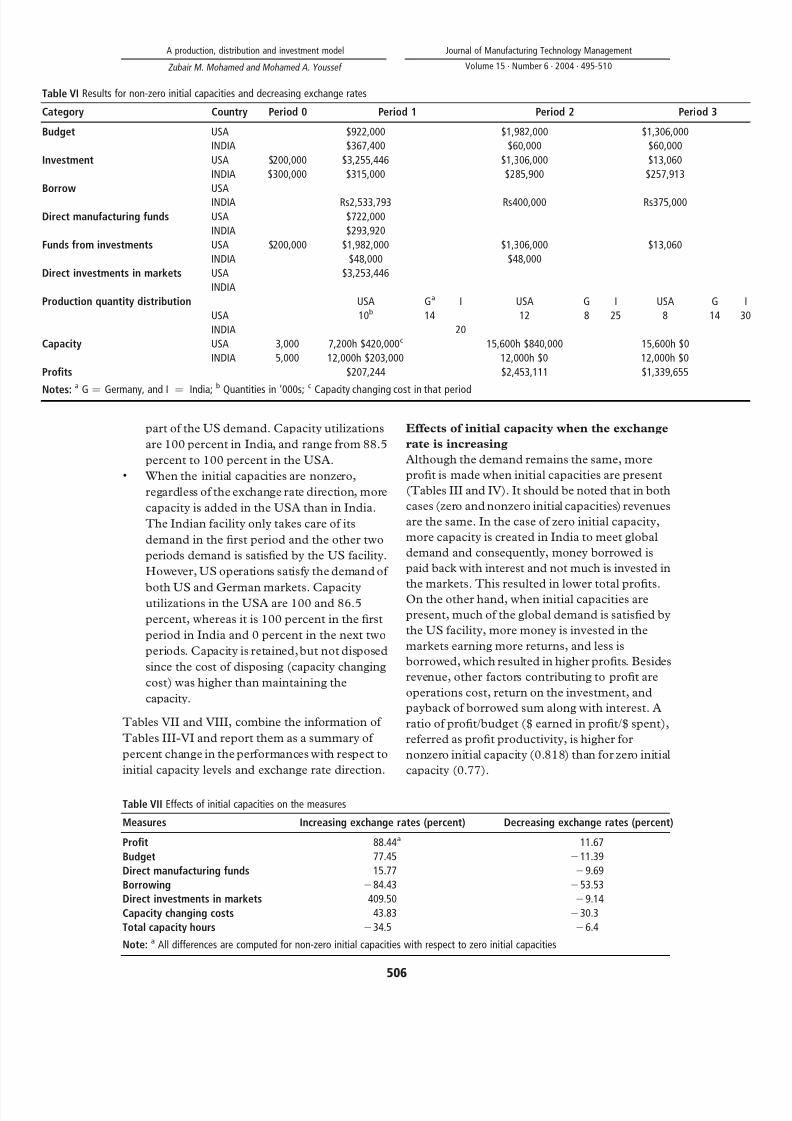
part of the US demand. Capacity utilizations

are 100 percent in India, and range from 88.5

percent to 100 percent in the USA.. When the initial capacities are nonzero,

regardless of the exchange rate direction, more

capacity is added in the USA than in India.

The Indian facility only takes care of its

demand in the first period and the other two

periods demand is satisfied by the US facility.

However, US operations satisfy the demand of

both US and German markets. Capacityutilizations in the USA are 100 and 86.5

percent, whereas it is 100 percent in the first

period in India and 0 percent in the next two

periods. Capacity is retained, but not disposed

since the cost of disposing (capacity changing

cost) was higher than maintaining the

capacity.

Tables VII and VIII, combine the information of

Tables III-VI and report them as a summary of

percent change in the performances with respect to

initial capacity levels and exchange rate direction.

Effects of initial capacity when the exchange

rate is increasing

Although the demand remains the same, more

profit is made when initial capacities are present

(Tables III and IV). It should be noted that in both

cases (zero and nonzero initial capacities) revenues

are the same. In the case of zero initial capacity,

more capacity is created in India to meet global

demand and consequently, money borrowed is

paid back with interest and not much is invested in

the markets. This resulted in lower total profits.On the other hand, when initial capacities are

present, much of the global demand is satisfied by

the US facility, more money is invested in the

markets earning more returns, and less is

borrowed, which resulted in higher profits. Besides

revenue, other factors contributing to profit are

operations cost, return on the investment, and

payback of borrowed sum along with interest. A

ratio of profit/budget ($ earned in profit/$ spent),

referred as profit productivity, is higher for

nonzero initial capacity (0.818) than for zero initial

capacity (0.77).

Table VI Results for non-zero initial capacities and decreasing exchange rates


Budget USA $922,000 $1,982,000 $1,306,000

INDIA $367,400 $60,000 $60,000

Investment USA $200,000 $3,255,446 $1,306,000 $13,060

INDIA $300,000 $315,000 $285,900 $257,913

Borrow USA

INDIA Rs2,533,793 Rs400,000 Rs375,000


INDIA $293,920

Funds from investments USA $200,000 $1,982,000 $1,306,000 $13,060

INDIA $48,000 $48,000


INDIA


USA 10b 14 12 8 25 8 14

INDIA 20

Capacity USA 3,000 7,200h $420,000c 15,600h $840,000 15,600h $0

INDIA 5,000 12,000h $203,000 12,000h $0 12,000h $0

Profits $207,244 $2,453,111 $1,339,655

Notes:a

G ¼ Germany, and I ¼ India;b

Quantities in ’000s;c

Capacity changing cost in that period

Table VII Effects of initial capacities on the measures

Measures Increasing exchange rates (percent) Decreasing exchange rates (percent)

Profit 88.44a 11.67

Budget 77.45 211.39

Direct manufacturing funds 15.77 29.69

Borrowing 284.43 253.53

Direct investments in markets 409.50 29.14

Capacity changing costs 43.83 230.3

Total capacity hours 234.5 26.4

Note: a All differences are computed for non-zero initial capacities with respect to zero initial capacities




Volume 15 · Number 6 · 2004 · 495-510

506

7/28/2019 851055


The effects of having nonzero initial capacities are

(Table VII): the profit increases by 88.44, the

budget increases by 77.45 percent, and direct

manufacturing funds in facilities increase by 15.77

percent. The direct investments in markets

increase by 409.5 percent to sustain budget

increase as the market investment is the primary

source of funding the budget and US facility is

more expensive to operate. Although fewer

capacity hours are needed when there is a

beginning capacity, the capacity changing cost is

higher as much of the manufacturing shifts from

India to the USA. When the initial capacities are

zero in both facilities, the decision calls for

producing more in the Indian facility,

consequently, more money is invested in the

Indian market. When the initial capacities are

nonzeros, much of the production takes place in

the US facility and no additional money is invested

further in the Indian market besides the initial

investment, although the return rate is much

higher in the Indian market (5-7 percent comparedto 1 percent in the US market).

Effects of initial capacity when the exchange

rate is decreasing

Regardless of the size of the initial capacity, much

of the manufacturing takes place in the US facility

which is more efficient but also more expensive.

The above discussions hold good here as well. The

profit productivity is 0.676 for zero initial

capacities and 0.852 for nonzero initial capacities.When the initial capacities are nonzeros, for the

same demand the profit increases by 11.67

percent, budget decreases by 11.39 percent, direct

manufacturing funds decrease by 9.6 percent,

direct investments in the market (US) decrease by

9.14 percent, capacity changing cost decreases by

30.3 percent, and 6.4 percent fewer capacity hours

are needed (Table VII). It should be noted that

besides the initial investment in the Indian market,

no further investment is made, although the return

rate is much higher compared to US market.

Effects of exchange rate direction when the

initial capacity is zero

More profit is made when the dollar is weaker

(decreasing exchange rate) than when it is

stronger. This is observed in reality and the reason

is that the revenues from foreign markets are

higher since more dollars are bought for the same

money. However, the profit productivity decreases

(0.676) as compared to when the dollar is stronger(0.77). This implies that if cost cutting measures

are undertaken, the productivity ratio can be

increased which should lead to even more higher

profits. In other words, instead of being satisfied

with higher profits by virtue of a weaker dollar,

more gains can be realized in this environment by

cutting down costs. When the dollar is weaker, the

following percent changes with respect to a

stronger dollar take place (Table VIII):. the budget increases by 100.26 percent as

much of the manufacturing shifts to the USA,

requiring 20.73 percent less hours as the US

facility is more efficient;. although the demand does not change, the

profit increases by 75.65 percent;. borrowing from the Indian market decreases

by 42.17 percent since not much is being

produced in India; and. the capacity changing cost increases by 122.77

percent as more expensive capacity is created

in the USA.

Effects of exchange rate direction when the

initial capacity is non-zero

Regardless of the exchange rate direction, much of the production takes place in the USA. More profit

is made when the dollar is weaker. The profit

productivity ratio is 0.818 for a stronger dollar and

0.852 for a weaker dollar. As before, this number

(i.e. 0.852) can be further improved by taking

advantage of a weaker dollar by cutting costs. As

the difference in the values of profit productivity

ratios is small, consequently, the effect on the

measures is not as pronounced as it was before

(zero initial capacity case). The budget remains

unchanged (Table VIII), direct manufacturing

Table VIII Effects of exchange rate direction on the measures

Measures Zero initial capacities (percent) Non-zero initial capacities (percent)

Profit 75.65a 4.08

Budget 100.26 0

Direct manufacturing funds 1.29 220.99

Borrowing 242.17 72.6

Direct investments in markets 497.18 6.5Capacity changing costs 122.77 7.92

Total capacity hours 227.03 4.33

Note: a All differences are computed for decreasing exchange rates with respect to increasing exchange rates




Volume 15 · Number 6 · 2004 · 495-510

507

7/28/2019 851055


funds decrease by 20.99 percent, direct

investments in the US market increase by 6.5

percent, no money is invested in the Indian

market, capacity changing costs increase by 7.92

percent, capacity hours needed increase by 4.33

percent, and the profit increases by 4.08 percent.

Although the effects may not be pronounced,

nonetheless they imply that when the exchangerate is decreasing ($ becoming weaker), there is a

potential for higher profits. This is also seen to

occur in reality. For example, a recent article

reports that MNCs in the USA earned a higher

profit in the first quarter due to the weaker dollar.

Earnings growth for MNCs in the first quarter of

1995 over the first quarter of 1994 has been 23

percent. This compares to 19 percent earnings

growth for the Standard and Poor’s 500 for all of

1994 (Daily News, 1995, p. 12-A).

Reality checksModels are essential for planning the supply chain

(Schary and Skjott-Larson, 2001). The only

prescription where there are no guidelines for

managers is to experiment (Eisenhardt and Brown,

1998), testing variables to see what happens. As

Schrage (2000) points out “We shape our models

and they shape our perception.” Breitman and

Lucas (1987) were first one to report the use of

PLANETS, a global supply chain management

model developed by General Motors for their use.

Lee and Billington (1995) and Lee et al. (1993)

describe the implementation of series of supply

chain management models at Hewlett-Packard.

Arntzen et al. (1995) report on the development

and use of a global supply chain model by the

Digital Equipment Corporation that saved them

over $100 million. Although we would like to

corroborate our model with a real life application,

so far we have not been successful in our attempts

in securing a firm to use our model. However, our

discussions with Mr Don Vitale, ex-CEO of DESA

International Corporation, Bowling Green,

Kentucky, have been very encouraging. He noted

that our model could certainly benefit DESA

Corporation. Since we were not able to apply our

model in a real life setting, we would like to depend

on the published qualitative research.Here, we would like to discuss how our model

results compare with the findings of Ferdows

(1997). The findings of Ferdows are based on his

four-year study of the role of foreign factories

owned by ten large multinational manufacturing

companies: Apple, Digital Equipment, Electrolux,

Ford, Hewlett-Packard, Hydro Aluminum, IBM,

Olivetti, Philips, and Sony. Also, his observations

are based on his work as a consultant for 12 large

MNCs, and on the data from several surveys that

he helped to conduct:

. US MNC’s earned higher profits due to

weaker dollar that our model also predicts.. Foreign factories with low wages after

adjusting for productivity and exchange rates

lose their attraction. Many US and European

electronics manufacturer turned some of their

off-shore facilities in Malaysia into server

facilities. Our model also predicts this as muchof the production shifts from India to the USA

when the Indian facility loses its low cost

advantage when exchange rates and

productivity makes it more expensive.. Fluctuations in foreign currencies turn offshore

facilities into servers. In our model, the Indian

facility is used more as a server facility.. Companies shift production rapidly to keep

costs down as currencies fluctuate. This is also

seen in our model results.

The agreement between the reality and model

results validates our model. Our future studies willaddress issues such as: do different exchange rate

theories affect the model outcomes significantly? If

the investment decision is excluded, would it affect

the results significantly? What conditions will favor

an off-shore facility or other facility types? When to

turn an off-shore facility into other facility types?

5. Conclusions

The supply chain planning contributes to

corporate planning. The role of these models is to

provide a rational basis for developing andevaluating strategic options (Schary and Skjott-

Larson, 2001). The supply chain plan includes

supply structure, markets, country and regional

constraints including exchange rates, custom duty,

capacity and transport capability, internal

elements of production capacity, etc.

The production, distribution, and investment

decisions are interrelated. The exchange rate

direction and initial capacity levels have pronounced

effects on these decisions. Investments in the

markets are done to support the production and

distribution activities. When the exchange rate

increases, a higher percent of money is borrowedfrom the local market to sustain operations. The

percent amount borrowed depends on the exchange

rate and not on the initial capacities or demand.

Changes in the exchange rate influence the activities

of both US and Indian facilities, and also on the

investments in the markets. The potential to make

higher profits depends on the initial capacity levels

and the exchange rates. Both of them have

pronounced effects on the profits. More profits can

be made by having nonzero initial capacities and

decreasing exchange rates ($ becoming weaker).




Volume 15 · Number 6 · 2004 · 495-510

508

7/28/2019 851055


References

Arntzen, B.C., Brown, G.C., Harrison, T.P. and Travton, L.L.(1995), “Global supply-chain management at digitalequipment corporation”, Interfaces , Vol. 25 No. 1,pp. 69-93.

Axarloglou, K., Kouvelis, P. and Sinha, V. (1995), “Exchange rate

and the choice of production models in supplying foreignmarkets: an empirical investigation”, working paper, DukeUniversity, Durham, NC.

Berry, W.L., Schmitt, T.G. and Vollman, T.E. (1982), “Capacityplanning techniques for manufacturing control systems:information requirements and operational features”,Journal of Operations Management , Vol. 3 No. 1,pp. 13-25.

Blackstone, J.H. (1989), Capacity Management , South-WesternPublishing, Cincinnati, OH.

Breitman, R.L. and Lucas, J.M. (1987), “PLANETS: a modelingsystems for business planning”, Interfaces , Vol. 17,pp. 94-106.

Canel, C. and Khumawala, B.M. (1993), “International facilitieslocation: a heuristic solution procedure for the multi-

period uncapacitated case”, Proceedings of the Decision Sciences Institute Annual Meeting , pp. 365-7.

Canel, C. and Khumawala, B.M. (1996), “A mixed integerprogramming approach for the international facilitieslocation problem”, International Journal of Operations & Production Management , Vol. 16 No. 4, pp. 49-68.

Cohen, M.A. and Kleindorfer, P.R. (1993), “Creating valuethrough operations”, Perspectives in Operations Management , Kluwer Academic Press, Boston, MA,pp. 3-21.

Cohen, M.A. and Mallik, S. (1997), “Global supply chains:research and applications”, Production and Operations Management , Vol. 6 No. 2, pp. 193-210.

Cohen, M.A., Fisher, M. and Jaikumar, R. (1989), “Internationalmanufacturing and distribution networks: a normative

model framework”, in Ferdows, K. (Ed.), Managing International Manufacturing , Elsevier Science Publisher,North Holland, Amsterdam, pp. 67-92.

Czinkota, M.R., Ronkainen, I.A. and Moffet, M.H. (1994),International Business , The Dryden Press, New York, NY.

Daily News (1995), “Quarterly earnings reports even better thanhigh expectations”, 23 April, p. 12-A.

Dasu, S. and Li, L. (1994), “Optimal operating policies in thepresence of exchange rate variability”, working paper,UCLA, Los Angeles, CA.

Dasu, S. and Torre, J. (1993a), “Impact of market liberalization onmultinational networks: a study of the Latin Americanfiber industry”, working paper, UCLA, Los Angeles, CA.

Dasu, S. and Torre, J. (1993b), “Restructuring multiplantoperations under conditions of competitive variation,market liberalization, and differentiated governance”,working paper, UCLA, Los Angeles, CA.

Dornier, P., Ernst, R., Fender, M. and Kouvelis, P. (1998), Global Operations and Logistics: Text and Cases , Wiley, New York,NY.

Eisenhardt, K.M. and Brown, S.L. (1998), “Competing on theedge of chaos”, Long Range Planning , Vol. 31 No. 5,pp. 786-9.

Ferdows, K. (1997), “Making the most of foreign factories”,Harvard Business Review , pp. 73-88.

Ferdows, K. (2000), “Making the most of foreign factories”, inGarten, J.E. (Ed.), World Views , Harvard Business ReviewPress, Boston, MA.

Flipo, C.D. (2000), “Spatial decomposition for a multi-facilityproduction and distribution problem”, International Journal of Production Economics , Vol. 64, pp. 177-86.

Fortune (1997), “What is eating McDonald’s?”, 13 October,pp. 122-5.

Fortune (2001), “The world’s largest corporations”, 23 July, p. F1.Griffin, R.W. and Pustay, M.W. (2002), International Business: A

Managerial Perspective , 3rd ed., Prentice-Hall, Englewood

Cliffs, NJ.Harvey, J.T. (1996), “Orthodox approaches to exchange rate

determination: a survey”, Journal of Post-Keynesian Economics , Vol. 18, pp. 567-83.

Harvey, J.T. and Quinn, S.F. (1997), “Expectations and rationalexpectations in the foreign exchange market”, Journal of Economic Issues , Vol. 31 No. 2, pp. 615-22.

Heizer, J. and Render, B. (2000), Operations Management ,6th ed., Prentice-Hall, Englewood Cliffs, NJ.

HighBeam Research (2001), Survey of Current Business ,September, pp. 53-90.

Hoch, L.C. (1982), “Site selection for foreign operations”,Industrial Development , Vol. 151, pp. 7-9.

Hodder, J.E. and Jucker, J.V. (1982), “Plant location modeling forthe multinational firm”, Proceedings of the Academy of

International Business Conference on the Asia-Pacific Dimension of International Business , Honolulu.

Huchzermeier, A. and Cohen, M.A. (1996), “Valuing operationalflexibility under exchange rate risk”, Operations Research ,Vol. 44 No. 1, pp. 100-13.

Karakaya, F. and Canel, C. (1998), “Underlying dimensions of business location decisions”, Industrial Management & Data Systems , Vol. 98 No. 7, pp. 321-9.

Kirca, O. and Koksalan, M.M. (1996), “An integrated productionand financial planning model and an application”, IIE Transactions , Vol. 28, pp. 677-86.

Kogut, B. (1984), “Normative observations on the internationalvalue-added chain and strategic groups”, Journal of International Business Studies , pp. 151-67.

Kogut, B. (1985a), “Designing global strategies: comparative

and competitive value-added chains”, Sloan Management Review , Vol. 26, pp. 15-38.

Kogut, B. (1985b), “Designing global strategies: profiting fromoperating flexibility”, Sloan Management Review , Vol. 26,pp. 27-38.

Kogut, B. and Kulatilaka, N. (1994), “Operating flexibility, globalmanufacturing, and the option value of a multinationalnetwork”, Management Science , Vol. 40, pp. 123-39.

Kouvelis, P. and Sinha, V. (1994), “Production-related strategiesfor foreign market entry”, Proceedings of the Decision Sciences Institute Annual Meeting , pp. 1473-5.

Kouvelis, P. and Sinha, V. (1995), “Exchange rate and the choiceof production strategies in supplying foreign markets”,working paper, Duke University, Durham, NC.

Lee, H.L. and Billington, C. (1995), “The evolution of supply-

chain-management models and practice at Hewlett-Packard”, Interfaces , Vol. 25 No. 5, pp. 42-63.

Lee, H.L., Billington, C. and Carter, B. (1993), “Hewlett-Packardgains control of inventory and service through design forlocalization”, Interfaces , Vol. 23 No. 4, pp. 1-11.

List, J.A. and Catherine, Y. (2000), “The effects of environmentalregulations on foreign direct investment”, Journal of Environmental Economics and Management , Vol. 40 No. 1,pp. 1-20.

McDonald, A.L. (1986), “Of floating factories and matingdinosaurs”, Harvard Business Review , Vol. 64 No. 6,pp. 82-6.

Min, H. and Melachrinoudis, E. (1996), “Dynamic location andentry mode selection of multinational manufacturing




Volume 15 · Number 6 · 2004 · 495-510

509

7/28/2019 851055


Documents

851055