Embed Size (px)
Citation preview
A Study on Model-Based Performance Evaluation of Dependable Computer Systems
(ディペンダブルコンピュータシステムのモデルベース性
能評価に関する研究)
Dissertation submitted in partial fulfillment for the
degree of Doctor of Engineering
Chao Luo
Under the supervision of
Associate Professor Hiroyuki Okamura
Dependable Systems Laboratory, Department of Information Engineering,
Graduate School of Engineering, Hiroshima University, Higashi-Hiroshima, Japan
September 2015

iii
Abstract
Model-based performance evaluation is an analytical approach for quantifying
system performance indices by modeling the dynamic behavior of system as
stochastic processes. Queueing analysis and Markov modeling are typical meth-
ods for the model-based performance evaluation. Compared to simulation ap-
proach, the model-based approach can provide highly-accurate assesses of per-
formance measures. Therefore, this is commonly used to evaluate performance
criteria of the system in the presence of rare events such as system failures.
On the other hand, as software system is widely used in our daily lives, it
becomes more important to prevent fatal system failures in computer system
design. In other words, several dependability measures such as system reliability,
system availability and data integrity, should be estimated only from the design
of system architecture before starting the implementation. This approach is
called the model-based software performance analysis, which is one of the most
attractive topics even in software engineering.
In this thesis, we consider model-based performance evaluation of three kinds
of computer system; distributed database system, open-source software and
virtualized system, respectively.
Firstly, we focus on the performance evaluation of distributed database sys-
tems with conventional snapshot isolation (CSI) and prefix-consistent snapshot
isolation (PCSI) by considering the occurrence of communication failures be-
tween a master and replicas. We also revisit our probabilistic models for CSI
and PCSI with the restart scheme for the communication failure. We investigate
the effect of update interval of snapshot and restart timing for the communica-
tion with respect to the abort probability and system throughput.
Secondly, we turn our attention to the maintenance scheduling for open
source software products. Applying a patch is one of effective fault-tolerant
techniques. We consider an optimized patch management model from the per-
spective of users by applying an NHPP to the bug-discovery process. Also,
with analyzing the characteristic of open source software by applying software
reliability models, we predictively propose an optimal maintenance schedule for
user according to numerical illustrations.
Finally, we dedicate our interest to the performance evaluation of virtualized

iv
system with software rejuvenation. Concretely, we evaluate the virtualized sys-
tem by using the criterion of resiliency, which is an attitude for measuring the
deviation of system when changes happen. We present MRSPNs (Markov re-
generative stochastic Petri nets) for the virtualized system with cold and warm
software rejuvenation and employ the technique of transient analysis through
PH (phase-type) expansion. This technique can reduce MRSPNs to a CTMC
approximately. After applying PH expansion to MRSPNs for the virtualized
system with software rejuvenation, we present the quantitative measure to eval-
uate the system resiliency based on CTMC analysis.


vii
Acknowledgements
First and foremost, I would like to extend my sincere gratitude to my supervisor
Associate Professor Hiroyuki Okamura for leading me into the world of proba-
bilistic modeling and helping me all through the term of this thesis. Without
his guidance and advices, the completion of this thesis would not have been
possible.
Also, my thanks go to Professor Tadashi Dohi and Professor Satoshi Fujita,
for their useful suggestions and checking the manuscript.
Finally, it is my special pleasure to acknowledge the hospitality and encour-
agement of the past and present members of the Dependable Systems Labora-
tory, Department of Information Engineering, Hiroshima University.


Contents
Abstract iii
Acknowledgements vii
1 Introduction 1
1.1 Optimization of Prefix-consistent Snapshot Isolation . . . . . . . 1
1.2 Maintenance Strategy of Open Source Software . . . . . . . . . . 3
1.2.1 Related Works . . . . . . . . . . . . . . . . . . . . . . . . 4
1.3 Resiliency of Virtualized Systems . . . . . . . . . . . . . . . . . . 6
1.4 Organization of Dissertation . . . . . . . . . . . . . . . . . . . . . 8
2 Performance Evaluation of Snapshot Isolation in Distributed
Database System 11
2.1 Database Management System . . . . . . . . . . . . . . . . . . . 12
2.2 Latency Distribution in Failure-Prone Environment . . . . . . . . 13
2.3 Conventional snapshot isolation (CSI) model . . . . . . . . . . . 17
2.4 Prefix-consistent snapshot isolation (PCSI) . . . . . . . . . . . . 21
2.5 Numerical Experiments . . . . . . . . . . . . . . . . . . . . . . . 25
2.5.1 Distribution Assumption . . . . . . . . . . . . . . . . . . . 26
2.5.2 Response Time . . . . . . . . . . . . . . . . . . . . . . . . 27
2.5.3 System Throughput . . . . . . . . . . . . . . . . . . . . . 30
2.5.4 Simulations . . . . . . . . . . . . . . . . . . . . . . . . . . 31
3 Optimal Planning for Open Source Software Updates 35
3.1 Bug-Correction Process . . . . . . . . . . . . . . . . . . . . . . . 35
3.2 Maintenance Cost Model . . . . . . . . . . . . . . . . . . . . . . . 37
3.3 Optimal Update Scheduling . . . . . . . . . . . . . . . . . . . . . 39
ix

x CONTENTS
3.3.1 Periodic Policy . . . . . . . . . . . . . . . . . . . . . . . . 40
3.3.2 Aperiodic Policy . . . . . . . . . . . . . . . . . . . . . . . 41
3.4 Numerical Examples . . . . . . . . . . . . . . . . . . . . . . . . . 43
3.4.1 Characteristic Analysis . . . . . . . . . . . . . . . . . . . 43
3.4.2 Real Data Analysis . . . . . . . . . . . . . . . . . . . . . . 45
4 Quantifying Resiliency of Virtualized System with Software Re-
juvenation 51
4.1 Virtualized System with Software Rejuvenation . . . . . . . . . . 51
4.2 MRSPN-based Analysis . . . . . . . . . . . . . . . . . . . . . . . 53
4.2.1 MRSPN Modeling . . . . . . . . . . . . . . . . . . . . . . 53
4.2.2 Transient Analysis . . . . . . . . . . . . . . . . . . . . . . 56
4.3 Quantification of System Resiliency . . . . . . . . . . . . . . . . . 58
4.4 Experiment . . . . . . . . . . . . . . . . . . . . . . . . . . . . . . 59
5 Conclusions 67
5.1 Summary and Remarks . . . . . . . . . . . . . . . . . . . . . . . 67
5.2 Future Works . . . . . . . . . . . . . . . . . . . . . . . . . . . . . 69
Appendix A EM-based PH fitting 71
Bibliography 74
Publication List of the Author 83


Chapter 1
Introduction
Model-based performance evaluation is an analytical approach for quantifying
system performance indices by modeling the dynamic behavior of system as
stochastic processes. Queueing analysis and Markov modeling are typical meth-
ods for the model-based performance evaluation. Compared to simulation ap-
proach, the model-based approach can provide highly-accurate assesses of per-
formance measures. Therefore, this is commonly used to evaluate performance
criteria of the system in the presence of rare events such as system failures.
On the other hand, as software system is widely used in our daily lives, it
becomes more important to prevent fatal system failures in computer system
design. In other words, several dependability measures such as system reliability,
system availability and data integrity, should be estimated only from the design
of system architecture before starting the implementation. This approach is
called the model-based software performance analysis, which is one of the most
attractive topics even in software engineering.
In this thesis, we consider model-based performance evaluation of three kinds
of computer system; distributed database system, open-source software and
virtualized system, respectively.
1.1 Optimization of Prefix-consistent SnapshotIsolation
In database system including distributed database system, there are four prop-
erties; (atomicity, consistency, isolation, durability), to guarantee the data in-
tegrity of database.[28] Atomicity property guarantees each transaction handled
1

2 CHAPTER 1. INTRODUCTION
entirely instead of partially. Consistency property ensures that any transaction
will bring the database from one valid state to another. Isolation property is
defined as invisibility of operations of a transaction to the other transactions.
Durability property guarantees that transactions that have committed will sur-
vive permanently. Since the isolation property critically affects throughput of
transactions in database system, we should take account of the trade-off be-
tween isolation level and system performance. When attempting to maintain
the highest level of isolation, a DBMS usually acquires locks on data which may
result in a loss of concurrency. The most basic implementation of the isolation
is based on a lock of data when it is read or written. However, it is known
that the lock-based isolation adversely affects the performance of database sys-
tem. Recent DBMSs adopt a more effective method using snapshot, so-called
snapshot isolation.[9] In the snapshot isolation, each transaction makes a copy
(snapshot) of the data at the beginning of a transaction, and updates the data
on the snapshot, instead of the original data. After the update operation, each
transaction sends a request for updating the original data, the DBMS processes
the requests according to the first-committer-wins rule. It has an advantage of
the abort probability of a transaction to the lock-based isolation. As a novel iso-
lation scheme, snapshot isolation has received much attention in various fields.
Ramesh et al. have implemented snapshot isolation for achieving atomicity in
multi-row transactions using RDBMS.[56] Also, snapshot isolation has been uti-
lized for management of scalable transactions on cloud computing platforms.[52]
On the other hand, since the snapshot isolation causes an overhead for get-
ting snapshot, the performance seriously degrades in the case of the system
with large latency for getting snapshot such as distributed database system. To
overcome this problem, Elnikety et al. proposed generalized snapshot isolation
to mitigate the overhead for getting snapshot.[18] Concretely, they presented
an implementation of generalized snapshot isolation called a prefix-consistent
snapshot isolation (PCSI), which periodically updates snapshot for a fixed time
interval, and examined the effectiveness of PCSI through the simulation study.
Bernabe-Gisbert and Zuikeviciute also discussed the performance of PCSI based
on a model.[10] They examined that PCSI improved response time for a trans-
action. On the other hand, PCSI essentially degrades system throughput and
1.2. MAINTENANCE STRATEGY OF OPEN SOURCE SOFTWARE 3
abort probability of a transaction unless the time interval for updating snap-
shot is optimized. Neither of [18] and [10] discussed such the optimization of
the design parameters of PCSI.
1.2 Maintenance Strategy of Open Source Soft-
ware
Nowadays, as well as the growing scale of software, the development cost is
rapidly increasing. Enterprises and individuals incline to update software in-
stead of purchasing new products. Therefore, the life cycle of software gets
longer and the burdens of maintenance and modification become significant. At
the same time, open source software becomes popular because of the price and
the modifiability. Many communities have been comprised for better communi-
cations between developers and users, and it also leads to swift feedbacks when
bugs or vulnerabilities are discovered. Combining these two aspects, we are
interested in the maintenance strategy of open source software.
The development of open source software is different from traditional soft-
ware. Traditional (closed source) software is usually developed by firms (ven-
dors) who are responsible for all the phases of software life cycle. That means
the maintenances and updates are provided by vendors unilaterally, even after
releasing. In the other hand, the quality enhancements of open source software
are promoted by both users and developers. Users have rights and interests
of reporting an experienced software failure to developers who are in charge of
modifying the potential bug related to the failure. Thus, the maintenance of
open source software can be thought as lots of bug fixes and several version-ups.
It is essentially the same as the maintenance of closed source software, but the
life cycle of open source software is much longer. The difference is, bugs are
reported by users not testers. However, from the point of view of bugs features,
there is few distinctions between open source and closed source software.
To be a user of open source software, besides reporting bugs to developers
after experiencing failures, they also have to keep their own duplication up-
to-date. The maintenance of open source software, however, are considered as
traditional means, i.e., patches and updates. A patch is a part of program
designed to fix bugs with, update a computer program or the supporting data,

4 CHAPTER 1. INTRODUCTION
and improve the usability or performance. One patch is always released by
vendor/developer with updates against one or several reported bugs or security
vulnerabilities. That is saying the patch releasing is strongly related with the
discoveries of bugs or vulnerabilities.
Generally, for the sake of reliability and security of software, patches should
be developed immediately users discover bugs. However, the development of
patches incur time and labor expenses for developers/vendors. For the closed
source software, vendors plan to release patches at a specified time interval,
and the patches fix all the bugs which have been discovered until the release
time. Due to the limitation of number of developers, the patches of open source
software cannot be developed as soon as the bugs discovered neither. That is
the motivation of discussion to the management of patches/updates.
Cavusoglu et al. have proposed a formulation for the cost of development and
distribution of patches, and also discussed the optimized periodic patch release
from the vendor perspective based on the cost function with respect to a steady-
state criterion.[14, 13] As previous research, Okamura et al. have discussed a
patch release strategy from the perspective of vendors by cost criterion.[47] Their
model assumed a NHPP as the number of discovered bugs and formulated the
expected total cost by considering the damage of exploit bugs before and after
a patch release. However, these papers have just discussed about what is the
best timing for releasing patches from the vendors’ angle. By investigating the
behavior of users, we can realize that not all patches are applied immediately
they are released. For convenience, users may occasionally apply patches even
it will bring much more risk of bug occurring. Also, less patch applying means
less cost of software update.
1.2.1 Related Works
In the past decades, software reliability models (SRMs), which describe and
analyze the software bug-discovery phenomenon, have been discussed in litera-
tures extensively.[36, 43] The classical and most important SRMs may be the
non-homogeneous Poisson process (NHPP) models developed by Goel and Oku-
moto, which describe the stochastic behavior of detecting potential bugs in the
test phase and predict the software reliability easily.[22] After that, Goel[23],

1.2. MAINTENANCE STRATEGY OF OPEN SOURCE SOFTWARE 5
Yamada et al.[70] and others[36, 42, 1] have proposed the different NHPP-based
SRMs. These SRMs are based on different debugging scenarios, and can qual-
itatively catch the software reliability growth phenomenon in test phases of
software products.
On the other hand, because the development of available patches are gov-
erned by bug-discovery and bug-correction processes, the consideration of bug-
correction process is essential for analyzing maintenance strategy of open source
software, particularly from users’ perspective. However, almost all the NHPP-
based SRMs assume the bug-correction process instantaneously, and only fo-
cus on the bug-discovery phenomenon. Schneidewind[59, 60] and Gokhale et
al.[24, 25] have discussed some concepts of software bug-correction phenomenon,
and explained the dependency between the bug-discovery/correction profiles
with analytical models and real data. Shibata et al.[61] have developed a novel
approach to analyze the software bug-discovery/correction processes simultane-
ously. Their idea to describe the bug-discovery/correction processes is to use
an Mt/M/∞ queueing model, where a fault is discovered and corrected by ex-
ponentially distributed random detection and repair times, respectively. Based
on queueing theory[11], they have assumed that the number of corrected bugs
can be modeled as an output process of an infinite server queue.
In addition, several mathematical models of patch management have been
proposed. Arora et al.[5] have considered the optimized plan for vulnerability
exposures over a software life cycle. Beattie et al.[7] have focused on the risk
that a patch re-injects a failure, and considered the optimal timing to apply
patches maximizing system availability. However, they have not dealt with the
properties of the discovery process. Cavusoglu et al. [14, 13] proposed the
patch release and management models from both vendor and user perspectives.
In addition, they discussed an equilibrium point of patch release times based
on a game theory between a vendor and a user. As an extension of Cavusoglu
et al.[14, 13], Okamura et al. have described a patch management model by using
non-homogeneous bugs-discovery process.[47] They have discussed an optimal
algorithm for minimizing the damage cost only from vendor perspective. Apart
from mathematical models, Brykczynski and Small reported practices of security
patch management, and also emphasized an importance of economic security

6 CHAPTER 1. INTRODUCTION
patch management as a part of information asset management.[12]
Moreover, we talk about the optimizing of maintenance scheduling. Marseguerra
et al. have presented an optimization approach based on the combination
of a Genetic Algorithms maximization procedure with a Monte Carlo simu-
lation, and a stochastic model of plant operation is developed from the stand-
point of its reliability/availability behavior.[39] Xia et al. have discussed the
maintenance scheduling with consideration of multi-attribute model (MAM).
They applied advance-postpone balancing (APB) and Maintenance time win-
dow (MTW) methods to utilize maintenance opportunities.[67, 68] Also, towards
the distributed energy system, they have developed a model-iteration algorithm
to optimize the maintenance schedule cycle by cycle.[69] Although these works
were done for hardware system, the methodologies for optimization of mainte-
nance schedule is worth to be referred.
1.3 Resiliency of Virtualized Systems
Virtualized system is one of the most flexible architectures to manage many
servers. In recent years, the virtualized system is used to build not only the
enterprise cloud system but also the private cloud which provides services for its
own staff in a small office. The virtualized system has the two-tier managements
for virtual machines (VMs) and virtual machine monitor (VMM). The VM is
an approach of virtualization which behaves as a real computer. It is to create
software components by emulating behavior of hardware units, and to control
them in a software platform. VM can make multiple OS environments without
redundant hardware cost. And a running virtual machine can be moved between
different physical machines without disconnecting the client. On the other hand,
VMM is the monitoring system to check behavior of VMs running on VMM. In
general, since administrators check VMs though VMM, the cost for management
can be reduced. In addition, VMM is generally installed on a physical machine,
and VMs shares the resources of physical machines such as CPU, memory and
network. Thus the virtual machine is also said to be good for the efficiency as
well as the management cost. However, although the maintenance for VMs is
easy in the virtualized system, it is not easy to make a maintenance plan for
VMM because VMM should continuously run while VMs provide their services.

1.3. RESILIENCY OF VIRTUALIZED SYSTEMS 7
That is, the aging phenomenon of VMM is serious problem in the virtualized
system.
In [37, 38], Machida et al. discussed software rejuvenation policies in a vir-
tualized system. The software rejuvenation is a proactive maintenance to avoid
the system failure caused by aging-related bugs.[29] The aging-related bugs are
defined as the bugs that cause the system performance degradation by long time
usage of the system. Typical examples of aging-related bugs are memory leak
and fragmentation. They are also reported on the virtualized platform such
as Xen. In general, it is difficult to find the root cause of aging-related bugs,
and we empirically know that the proactive maintenance such as reboot and
restarting processes is effective to prevent the system failure by aging-related
bugs. Such maintenance is generally called software rejuvenation.[31] The soft-
ware rejuvenation operation is often managed by a time-triggered policy, i.e.,
the system automatically execute the rejuvenation operation under scheduled
time. Machida et al.[37, 38] discussed the steady-state measures under three
kinds of rejuvenation policies called cold-VM, warm-VM and migrate-VM re-
juvenations in the virtualized system. Also, Okamura et al.[49] evaluated the
transient measures for the virtualized system with software rejuvenation.
The software aging is caused by the resource exhaustion with long-term
operation. On the other hand, it is also important to evaluate the system
performance when a suddenly change occurs in practice. The change includes
changes of system configuration and environments of system such as rate of
arrivals. The extreme example is a disaster like flood, fire and earthquake. To
avoid the worst scenario, it is useful to predict what happens in the system if the
system suffers such disasters. The resiliency is known as one of the attributes of
system to be evaluated for such changes. In brief, the resiliency is a resistance
of system for a change. In the research field of dependability computing, many
definitions of resiliency were proposed to characterize this concept. Laprie[33]
and Simoncini[62] defined the resiliency as the resistance of service delivery when
facing changes. In addition, based on this definition, Gohsh et al.[21] tried to
quantify the system resiliency in IaaS cloud through the modeling of system
with continuous-time Markov chains (CTMCs).

8 CHAPTER 1. INTRODUCTION
1.4 Organization of Dissertation
This thesis is organized as follows:
Firstly, in Chapter 2, we focus on the performance evaluation of conventional
snapshot isolation (CSI) and PCSI based on probabilistic models and discuss the
optimization of the design parameter of PCSI by using the probabilistic models
for the distributed database system. In [35], the model-based performance eval-
uation of CSI and PSCI with the optimization has been discussed. However,
[35] assumed that any failure did not occur during the communication between
a master and replicas. Generally, in distributed environment, communication
failures are non-negligible factors that negatively affect the performance of sys-
tems in the distributed environment. Thus, one of the purpose of this chapter is
to reveal the impact of communication failures to the system performance. Con-
cretely, this chapter revisits our probabilistic models for CSI and PCSI with the
restart scheme for the communication failure which discussed by van Moorsel
and Wolter.[40] We investigate the effect of update interval of snapshot and
restart timing for the communication with respect to the abort probability and
system throughput.
In Chapter 3, we consider a patch management model from the perspec-
tive of users by applying an NHPP to the bug-discovery process. We focus on
another part of the patch management game by Cavusoglu et al. from user
perspective.[14, 13] We expand the time-based patch release policy proposed by
Okamura et al. into a number-based policy and formulate the total cost from
user perspective.[47] Also, with analyzing the characteristic of open source soft-
ware by applying software reliability models, we predictively propose an optimal
updating schedule for user according to numerical illustrations.
In Chapter 4, we focus on the quantification of resiliency of the virtualized
system with software rejuvenation. Concretely, according to the manner of [21],
we evaluate the resiliency of the virtualized system. However, since Machida et
al.[37, 38] originally presented MRSPNs (Markov regenerative stochastic Petri
nets) for the virtualized system with software rejuvenation, we could not apply
the same approach as [21] to the virtualized system model directly. Then we em-
ploy the technique in [49], i.e., the transient analysis through PH (phase-type)

1.4. ORGANIZATION OF DISSERTATION 9
expansion. This technique can reduce MRSPNs to a CTMC approximately.
After applying PH expansion to MRSPNs for the virtualized system with soft-
ware rejuvenation, we present the quantitative measure to evaluate the system
resiliency based on CTMC analysis.
Finally, the thesis is concluded with some remarks and future directions in
Chapter 5.

10 CHAPTER 1. INTRODUCTION
Chapter 2
Performance Evaluation ofSnapshot Isolation inDistributed DatabaseSystem
Database systems are widely used in many fields. As the scale of database sys-
tems increases, more firms decide to deploy the database system in a distributed
environment for the sake of data integrity fault tolerance. For guaranteeing
the consistency of data, database management systems adopt isolation policies.
This chapter discusses probabilistic models for snapshot isolation of database
management system. Snapshot isolation is an effective method to enhance the
consistency of database system. Although, it degrades the system performance
where the system has large network latency such as distributed database system.
Also, under the failure-prone environment, a restart scheme is considered as one
countermeasure. This chapter proposes probabilistic models for the dynamics of
snapshot isolation of database system and exhibits the optimization of system
performance with respect to updating interval of snapshot isolation within the
failure-prone environment from the analytical point of view. Numerical exper-
iments are conducted to validate the effectiveness of analytical results by using
real traffic data.
11

12CHAPTER 2. PERFORMANCE EVALUATION OF SNAPSHOT ISOLATION
2.1 Database Management System
Database management system (DBMS) is a fundamental software to control
transactions that arrive at the database system. In DBMS, there are four
significant properties abbreviated as ACID (atomicity, consistency, isolation,
durability). The atomicity is the property ensuring that either all or none of
the operations have been executed when a transaction is completed. This cor-
responds to the commit/abort scheme. The consistency is to ensure that a
transaction does not change the database to any of inconsistent states whenever
the state of database is consistent at the beginning of the transaction. The
isolation is to make all the operations of a transaction invisible to other trans-
actions. The durability is to ensure that all the successful transactions must
persist even though a system failure occurs. In particular, since the isolation af-
fects the performance of database, four isolation levels are defined in ANSI/ISO
SQL standard; read uncommitted, read committed, repeatable reads and seri-
alizable. The serializable is the highest level of isolation. This level requests
starting and ending times of all the transactions to be serial in the execution
history of transactions. In this level, we prevent any of inconsistency such as
dirty reads, non-repeatable reads and phantom reads [9].
This chapter focuses on the serializable level of isolation. There are two
implementation schemes to achieve the serializable level. One method is the
lock-based control. In the lock-based control, DBMS acquires locks on the
data during the transaction is executed. The implementation of lock-based
control is simple. However, when a transaction spends long processing time,
the performance of database such as system throughput is drastically degraded,
since all the transactions that arrive in the processing time are canceled or
aborted. Another implementation is based on the version of database, called
the version-based control or the snapshot isolation (SI). In the SI, DBMS does
not acquire a lock on the data. Instead of locks, DBMS makes a snapshot of
database before starting a transaction, and checks write conflicts on the data
by using the snapshot at which each transaction is completed. That is, the
transaction that has no conflict with other transactions is only committed at
the termination (first-committer-wins rule [9]). Compared with the lock-based
control, the SI is expected to provide high system throughput.

2.2. LATENCY DISTRIBUTION IN FAILURE-PRONE ENVIRONMENT13
On the other hand, the SI poses a problem with response time overhead
to get the last snapshot. In the conventional snapshot isolation (CSI), since
DBMS should get the latest snapshot before processing a transaction, it can be
equated to the fact that the processing time of a transaction under the SI is
longer than that under the lock-based control. Specifically, in the case where the
SI is applied to distributed database system with a master server, the network
latency to get the latest snapshot should be considered as a part of response time.
To overcome this problem, Elnikety et al. [18] proposed the generalized snapshot
isolation (GSI) which allows us to use the ‘potentially’ latest snapshot. Under
the first-committer-wins rule, the first transaction committed on a snapshot is
a winner on the snapshot. Thus the probability of commit generally depends on
the age of snapshot at which the transaction starts. The probability of commit
with ‘young’ snapshot is higher than that with ‘older’ snapshot, because the
‘older’ snapshot is likely to be changed by other transactions. In other words, if
we could maintain a certain level of the probability of commit, it is not necessary
to use the latest snapshot. Elnikety et al. [18] focused on such the property of
SI, and proposed an implementation of GSI called prefix-consistent snapshot
isolation (PCSI) to enhance the response time. In the PCSI, the process to get
the latest snapshot is executed at every prefixed time interval. Figures 2.1 and
2.2 illustrate communication between the master and the replica in conventional
SI (CSI) and PCSI.
However, one of the transactions on the same snapshot may be committed
under the first-committer-wins rule. In the PCSI, a snapshot is used for all the
transactions that arrive during the prefixed time interval for updating snapshot,
namely, the number of transactions using the same snapshot in the PCSI is larger
than that in the CSI. It indicates that the system throughput of PCSI is lower
than that of CSI. This motivates us to consider the optimal time interval for
updating snapshot in the PCSI.
2.2 Latency Distribution in Failure-Prone Envi-
ronment
As shown in the previous section, Elnikety et al. [18] have extended the snapshot
isolation scheme to the distributed database system with innegligible latency of

14CHAPTER 2. PERFORMANCE EVALUATION OF SNAPSHOT ISOLATION
replica
master
arrival of a transaction
request for snapshot
processing time
request for commit
acknowledgement of commit/abort
time
completion of a transaction
Figure 2.1: Schematic illustration of conventional snapshot isolation.
replica
master
arrival of a transaction
request for snapshot
processing time
request for commit
acknowledgement of commit/abort
time
update interval
Figure 2.2: Schematic illustration of prefix-consistent snapshot isolation.
communication between replicas and master. Their scheme implicitly assumed
that a replica can get a response from the master with probability one. How-
ever, when we focus on the network/transmission layer in the network model,
this assumption does not hold in any network environment. M. Tamer Ozsu
et al. have discussed fundamental principles of distributed data management
and data management in different network architectures [51]. Though TCP
(transmission control protocol) equips the retransmission scheme to ensure the
end-to-end communication, the latency of communication strongly depends on
the communication environment. Richard L. Graham et al. have detailed the
features of an end-to-end network failure- tolerant message-passing system [27].
In particular, in the case of failure-prone environment, it is useful to design
both high and low layers by considering the effect of retransmission scheme in

2.2. LATENCY DISTRIBUTION IN FAILURE-PRONE ENVIRONMENT15
start restart restart completion
C (total completion time)
c c
restart time restart time
Figure 2.3: Possible sample path of the restart scheme.
low layer to the latency distribution in high layer. Hsieh et al. have studied
the maximum latency guarantee in networks [30]. In addition, the performance
model by Luo et al. [35] also assumed that the first moment of latency is finite.
If the probability that the communication failure occurs is not zero, the first
moment of latency becomes infinite. Thus we should consider the retransmission
scheme and snapshot isolation simultaneously in the model.
van Moorsel and Wolter [40] discussed the completion time under the general
restart scheme that can directly be applied to the retransmission scheme of the
Internet. According to the restart scheme [40], we first discuss the latency
distribution in the failure-prone environment.
Define the following random variables:
• L (> 0): the latency of communication from a sender to a receiver through
the network. This is a random variable having a cumulative distribution
function (c.d.f.) FL(t).
Since the communcation failure occurs in the failure-prone environment, the
c.d.f. of FL(t) is allowed to be defective, i.e., F (∞) < 1. Then the probability
of communication failure corresponds to 1− F (∞). Also, the first moment can
be defined by
E[L] =
∫ ∞
0
tdFL(t) =
∫ ∞
0
FL(t)dt, (2.1)
where, in general, F (·) = 1− F (·). Hence, when the probability of communica-
tion failure is not zero, the first moment of L, E[L] is not finite.
van Moorsel and Wolter [41] considered a general restart scheme. In their

16CHAPTER 2. PERFORMANCE EVALUATION OF SNAPSHOT ISOLATION
scheme, the sender waits for an acknowledgement from the receiver by the limit
τ (> 0). That is, if the sender does not get an acknowledgement from the receiver
until time unit τ , the sender resends a request to the receiver with the restart
overhead time c (> 0). The sender repeatedly sends requests until obtaining an
acknowledgement form the receiver. Figure 2.3 illustrates the possible sample
path under the restart scheme by van Moorsel and Wolter [41]. For the sake
of simplicity, the sender is assumed to be cancel the pervious request before
resending a new request. Let C be a completion time under such a restart
scheme. Then the c.d.f. of the completion time is given by
FC(t) = P (C ≤ t)
=
{
1− FL+L(τ)kFL+L(t− k(τ + c)), k(τ + c) ≤ t < k(τ + c) + τ
1− FL+L(τ)k+1, k(τ + c) + τ ≤ t < (k + 1)(τ + c).
(2.2)
In the above equation, FL+L indicates the c.d.f. of a round-trip time without
communication failure that is a 2-fold convolution of L;
FL+L(t) =
∫ t
0
FL(t− x)dFL(x). (2.3)
The expected time of the completion time holds the following equation:
E[C] =
∫ τ
0
E[C|C = x]dFL+L(x) +
∫ ∞
τ
(τ + c+ E[C])dFL+L(x)
=
∫ τ
0
xdFL+L(x) + (τ + c+ E[C])FL+L(τ). (2.4)
Then we have
E[C] =
∫ τ
0 FL+L(x)dx + cFL+L(τ)
FL+L(τ). (2.5)
From the above equation, we find that E[C] is always finite even if FL(∞) < 1.
Also the Laplace-Stieltjes (LS) transform of C can be derived from
E[e−sC ] =
∫ τ
0
E[e−sC |C = x]dFL+L(x) +
∫ ∞
τ
e−s(τ+c)E[e−sC ]dFL+L(x)
=
∫ τ
0
e−sxdFL+L(x) + e−s(τ+c)E[e−sC ]FL+L(τ), (2.6)
and
E[e−sC ] =
∫ τ
0e−sxdFL+L(x)
1− e−s(τ+c)FL+L(τ). (2.7)

2.3. CONVENTIONAL SNAPSHOT ISOLATION (CSI) MODEL 17
The completion time under the restart scheme can be represented by C =
(τ+c)NF +L1+L2, where NF is the number of restarts, L1 and L2 are latencies
for a request and an acknowledgement, respectively, provided that L1+L2 ≤ τ .
Letting P1 = (τ + c)NF + L1 and P2 = L2 provided that L1 + L2 ≤ τ , we have
E[P1] + E[P2] = E[P1 + P2] = E[C]. (2.8)
Also, the LS transforms of P1 and P2 are
E[e−sP1 ] = E[e−s(τ+c)NF ]× E[e−sL1 |L1 + L2 ≤ τ ]
=
∞∑
k=0
e−s(τ+c)kFL+L(τ)FL+L(τ)k × E[e−sL1 |L1 + L2 ≤ τ ]
=FL+L(τ)
1− e−s(τ+c)FL+L(τ)×
∫ τ
0
∫ t
0e−sxfL(t− x)dFL(x)dt
FL+L(τ)
=
∫ τ
0
∫ t
0 e−sxfL(t− x)dFL(x)dt
1− e−s(τ+c)FL+L(τ)=
∫ τ
0 e−stFL(τ − t)dFL(t)
1− e−s(τ+c)FL+L(τ)(2.9)
and
E[e−sP2 ] = E[L2|L1 + L2 ≤ τ ]
=
∫ τ
0
∫ t
0e−sxfL(t− x)dFL(x)dt
FL+L(τ)=
∫ τ
0e−stFL(τ − t)dFL(t)
FL+L(τ). (2.10)
It should be noted that E[e−sC ] 6= E[e−sP1 ]E[e−sP2 ] since P1 and P2 are not
mutually independent random variables.
2.3 Conventional snapshot isolation (CSI) model
Consider a distributed database system having a central server (master) and
several replicas. We suppose that all the replicas have a copy of the database
in the master. Thus, in the practical situation, the master and replicas should
execute the replication procedure such as 2-phase commit. However, since this
chapter focuses only on the performance of SI between the master and a replica,
we ignore the effect of a request message from the master to replicas. In addi-
tion, we consider only the arrival stream of update transactions, because read
transactions are never aborted in the scheme of SI and there is no effect of read
transactions to the performance.
Define the following random variables:

18CHAPTER 2. PERFORMANCE EVALUATION OF SNAPSHOT ISOLATION
• C (> 0): the latency of communication between the master and a replica
with the restart scheme described in Section 3. Similar to Section 3, we
decomposes the total latency C as C = C1 + C2, where C1 is the time
for the request arrives at the master and C2 is the time required from the
master to the replica. Note that the time C1 includes canceled requests
by restarts.
• T (> 0): the time spent by a transaction (random variable having a c.d.f.
FT (t)).
Suppose that the arrival stream of update transactions to a replica is a Poisson
process with rate λR, i.e., the inter-arrival time of update transactions is given
by an exponential distribution with mean 1/λR. When a new transaction arrives
at the replica, the replica requests the latest snapshot to the master.
The total time for executing all the operations of a transaction is given by T
having the c.d.f. FT (t). After completing all the operations, the replica sends a
message of request for commit to the master. Similar to the request for snapshot,
the latency for the commit request is also given as the round-trip time C.
On the other hand, the master receives requests for commit from the other
replicas in accordance with a Poisson process with rate λA. According to the
first-committer-wins rule, the master decides a request for commit is committed
or aborted. Concretely, in the CSI scheme, if no commit occurs during the
latencies and processing time of a transaction, the transaction is committed.
Otherwise, if one or more transactions are committed during the latencies and
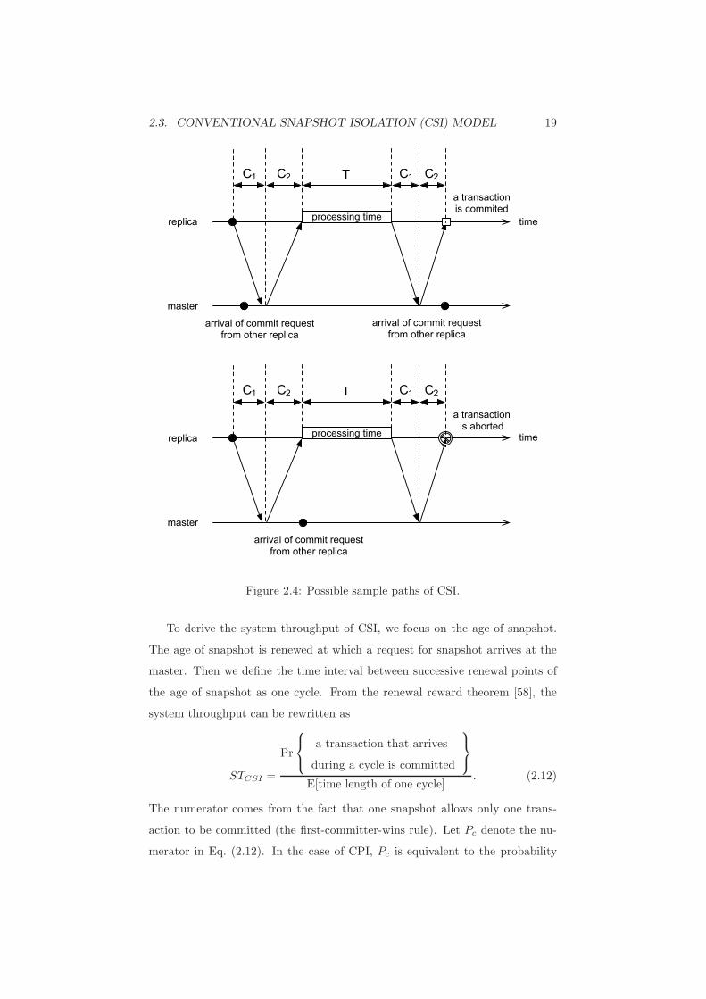
the processing time, the transaction is aborted. Figure 2.4 depicts possible
sample paths when transactions are aborted and committed.
Next we derive the performance measures in CSI model. This chapter con-
siders system throughput, abort probability and response time as criteria of
performance on the distributed database system. The system throughput is
defined as the number of committed transactions per unit time, i.e.,
ST = limt→∞
E
the number of committed
transactions during [0, t)
t. (2.11)
The system with high throughput is better than the system with low throughput.
2.3. CONVENTIONAL SNAPSHOT ISOLATION (CSI) MODEL 19
replica
master
processing timetime
C1 C2 C1 C2T
arrival of commit requestfrom other replica
replica
master
processing time time
C1 C2 C1 C2T
arrival of commit requestfrom other replica
a transactionis aborted
a transactionis commited
arrival of commit requestfrom other replica
Figure 2.4: Possible sample paths of CSI.
To derive the system throughput of CSI, we focus on the age of snapshot.
The age of snapshot is renewed at which a request for snapshot arrives at the
master. Then we define the time interval between successive renewal points of
the age of snapshot as one cycle. From the renewal reward theorem [58], the
system throughput can be rewritten as
STCSI =
Pr
a transaction that arrives
during a cycle is committed
E[time length of one cycle]. (2.12)
The numerator comes from the fact that one snapshot allows only one trans-
action to be committed (the first-committer-wins rule). Let Pc denote the nu-
merator in Eq. (2.12). In the case of CPI, Pc is equivalent to the probability
20CHAPTER 2. PERFORMANCE EVALUATION OF SNAPSHOT ISOLATION
that the first transaction is committed, i.e., we consider the probability that
C2 +T +C1 is faster than the arrival time of the request for commit from other
replicas. Here, in general, the probability that a random variable X having a
c.d.f. F (t) is lower than an exponentially distributed random variable Y with
mean 1/λ is given by∫ ∞
0
λe−λtP (X ≤ t)dt = λ
∫ ∞
0
e−λtF (t)dt = F ∗(λ), (2.13)
where F ∗(s) is the LS transform of F (t), namely,
F ∗(s) =
∫ ∞
0
e−λsdF (t). (2.14)
From the LS transforms of C2 and C1, we have
Pc =
∫ ∞
0
λAe−λAtP (C2 ≤ t)dt
∫ ∞
0
λAe−λAtP (T ≤ t)dt
×
∫ ∞
0
λAe−λAtP (C1 ≤ t)dt
=F ∗C1(λA)F
∗C2
(λA)F∗T (λA), (2.15)
where F ∗C1(s) = E[e−sP1 ] and F ∗C2
(s) = E[e−sP2 ] are defined as Eqs. (2.9) and
(2.10). Also, the expected time length of one cycle is given by E[C2 + T +C1 +
C2 +XA + C1], where XA is a random variable representing the time when a
new transaction arrives at the replica after receiving the acknowledgement of a
commit request. From the memoryless property of exponential distribution, we
get E[XA] = 1/λR. Then the system throughput of CSI can be obtained by
STCSI =F ∗C1
(λA)F∗C2
(λA)F∗T (λA)
2E[C] + E[T ] + 1/λR
. (2.16)
Since the arrival rate of transaction λR is defined as the number of transac-
tions per unit time, the abort probability of a transaction is obtained by using
the system throughput, i.e.,
APCSI = 1−STCSI
λR
. (2.17)
Also, the response time is defined by the expected time until receiving the
acknowledgement for a commit request from starting operations of a transaction.
Then we have
RTCSI = E[C1 + C2 + T + C1 + C2]
= 2E[C] + E[T ]. (2.18)

2.4. PREFIX-CONSISTENT SNAPSHOT ISOLATION (PCSI) 21
Remark 4.1 (Non-homogeneous Poisson process): Non-homogeneous
Poisson process (NHPP) is also considerable for the arrivals in master. NHPP is
widely used for describing numerous random phenomena in many fields. How-
ever, it augments the difficulty of derivation of formulations and the computation
complexity. Thus, we consider Poisson process in this chapter.
2.4 Prefix-consistent snapshot isolation (PCSI)
Similar to the model of CSI, we consider the database with a master and replicas.
The update transactions that arrive at a replica are according to a Poisson
process with rate λR, and the requests for commit to the master follows a
Poisson process with mean λA. Moreover, we define the random variables that
the latency of communication (round-trip time) C and the processing time of a
transaction T under the failure-prone environment. The c.d.f.s of C and T are
also given by FC(t) and FT (t), respectively. According to the restart scheme of
van Moorsel and Wolter [41], the c.d.f. of C can be presented in Eq. (2.2) with
the restart timing and overhead τ and c. Also the latency is divided into C1
and C2 which are latency from a replica to the server and from the server to a
replica under the restart scheme.
In the PCSI, the snapshot in the replica is updated when the age of snapshot
exceeds U . The age of snapshot is larger when the time interval of updating
snapshot is longer. On the other hand, the short update interval causes the
overhead to obtain the snapshot from the master. Furthermore, we assume that,
if the time until receiving an acknowledgment exceeds update interval U , the
updating snapshot is delayed to the time until receiving the acknowledgement.
Figure 2.5 illustrates sample paths of our PCSI model.
Consider the performance measures in the PCSI. From the renewal reward
theory, the system throughput of PCSI can also be defined as Eq. (2.11). Define
a cycle as time interval between two successive renewal points of the age of
snapshot. Then the system throughput under the PCSI is given by
STPCSI =
Pr
a transaction that arrives
during a cycle and it is committed
E[time length of one cycle]. (2.19)

22CHAPTER 2. PERFORMANCE EVALUATION OF SNAPSHOT ISOLATION
replica
master
processing timetime
C1 C2 C13 C2T
U
replica
master
processing time time
C1 C2 C1 C2T
U
arrival of commit request from other replica
arrival of commit request from other replica
a transaction is commited
arrival of commit request from other replica
a transaction is aborted
Figure 2.5: Possible sample paths of PCSI.
First we consider the probability that a transaction arriving in a cycle is com-
mitted. Let Pp(U) be the numerator of Eq. (2.19) because the probability is a
function of time interval for updating snapshot U . Since the inter-arrival time
2.4. PREFIX-CONSISTENT SNAPSHOT ISOLATION (PCSI) 23
of transactions is given by an exponential random variable, we obtain
Pp(U) =
∫ U
0
λRe−λRte−λAtdt
×
∫ ∞
0
λAe−λAtP (C1 ≤ t)dt
×
∫ ∞
0
λAe−λAtP (C2 ≤ t)dt
×
∫ ∞
0
λAe−λAtP (T ≤ t)dt
=λR
λR + λA
(
1− e−(λR+λA)U)
F ∗C1(λA)F
∗C2
(λA)F∗T (λA). (2.20)
Next we derive the expected time of one cycle. Let Cp(U) denote the expected
time of one cycle. For the notational simplification, G(t) is the c.d.f. of the
random variable T + C1 + C2 = T + C since C1 and C2 belong to the same
round trip. In other words, G(t) can be obtained by the inverse LS transform
of the following LS transform:
G∗(s) = F ∗T (s)F∗C(s) = F ∗T (s), (2.21)
where
F ∗C(s) = E[e−sC ] =
∫ τ
0 e−sxdFL+L(x)
1− e−s(τ+c)FL+L(τ). (2.22)
As mentioned before, system automatically renews the snapshot in U time in
case transactions terminated before time interval U . However, it is possible that
transactions are being processed until U time. For this situation, we assume
system does not update the snapshot until the accomplishment of transactions,
i.e., one cycle is considered as the period from prior snapshot to the end of
delayed transactions. Then the expected time of one cycle is given by
Cp(U) = E[C2]
+
∫ U
0
(
UG(U − t) +
∫ ∞
U−t
sdG(s)
)
λRe−λRtdt
+ Ue−λRU + E[C1]
= U + E[C] + (E[T ] + E[C])(1 − e−λRU )
−
∫ U
0
G(s)(1 − e−λR(U−s))ds, (2.23)
where G(s) = 1−G(s). Then the system throughput becomes
STPCSI(U) =Pp(U)
Cp(U). (2.24)

24CHAPTER 2. PERFORMANCE EVALUATION OF SNAPSHOT ISOLATION
Also, the abort probability of a transaction and the response time can be ob-
tained as follows.
APPCSI(U) = 1−STPCSI(U)
λR
, (2.25)
RTPCSI = E[T + C1 + C2] = E[C] + E[T ]. (2.26)
Note that the response time of PCSI does not depend on the time interval for
updating the snapshot U .
As mentioned before, the system throughput of the PCSI is always less than
that of CSI. In addition, the system throughput changes with the time interval
for updating snapshot U . Therefore, in the design of PCSI, it is important
to find the optimal update interval maximizing the system throughput. This
chapter presents an analytical result on the optimal update timing in the PCSI
scheme.
Consider the first derivatives of Pp(U) and Cp(U) with respect to U . Then
we have
d
dUPp(U) = λRe
−(λR+λA)UF ∗C1(λA)F
∗C2
(λA)F∗T (λA) (2.27)
and
d
dUCp(U) =1 + (E[T ] + E[C])λRe
−λRU
−
∫ U
0
G(s)λRe−λR(U−s)ds. (2.28)
Here we define the function q(U) which is the numerator of the first derivative
of STPCSI(U):
q(U) = Cp(U)d
dUPp(U)− Pp(U)
d
dUCp(U). (2.29)
Then we have the following result on the optimal update timing:
Theorem: There is a unique and finite solution of U∗ maximizing the system
throughput such that q(U∗) = 0 in the PCSI scheme under the restart scheme.
The maximum throughput is given by
STPCSI(U∗) =
e−(λR+λA)U∗
F ∗C1(λA)F
∗C2
(λA)F∗T (λA)
(1/λR)(1 − Pe(U∗)) + (E[C] + E[T ])e−λRU∗, (2.30)

2.5. NUMERICAL EXPERIMENTS 25
where Pe(U) is the probability that a transaction arrives during U and the time
receiving the acknowledgement for a commit request exceeds the time for updating
snapshot U ; Pe(U) =∫ U
0G(U − s)λRe
−λRsds.
Proof: Consider the function q(U) = e−(λR+λA)Uq(u), which has the same sign
of the first derivative of STPCSI(U) with respect to U . Then we get
d
dUq(U) = −λRλAe
(λR+λA)U
(
1
λR
(1− Pe(U))
+1
λA
G(U) + (E[C] + E[T ])e−λRU
)
Pp(U). (2.31)
It is straightforward to find dq(U)/dU < 0 for any U . Hence the function q(U)
is a monotonically decreasing function of U . From Eqs. (2.19)– (2.29), we have
q(0) = λRF∗C1
(λA)F∗C2
(λA)FT (λA)Cp(0) > 0 (2.32)
and
q(∞) =− Pp(∞)
=−λR
λR + λA
F ∗C1(λA)F
∗C2
(λA)F∗T (λA) < 0. (2.33)
The sign of q(U) is equal to the sign of the first derivative of STPCSI(U), and
henceforth, STPCSI(U) is a concave function having a global maximum point
U∗ such that q(U∗) = 0. Also, from q(U∗) = 0, the maximum throughput can
be obtained:
STPCSI(U∗) =
Pp(U∗)
Cp(U∗)=
ddU
Pp(U)∣
∣
U=U∗
ddU
Cp(U)∣
∣
U=U∗
. (2.34)
From the above theorem, we find that there exists a unique optimal update tim-
ing U∗ which minimizes the abort probability, and the optimal update timings
in terms of system throughput and abort probability are identical.
2.5 Numerical Experiments
In this section, we present numerical examples for the system throughput of
CSI and PCSI under the failure-prone environment. We examine how much the
system throughput of PCSI decreases compared to CSI. As mentioned before,

26CHAPTER 2. PERFORMANCE EVALUATION OF SNAPSHOT ISOLATION
although the response time of PCSI is improved, the system throughput of PCSI
is less than that of CSI. Thus we investigate the effectiveness of determining the
optimal time interval for updating snapshots in PCSI.
2.5.1 Distribution Assumption
Suppose that the latency of communication between a replica and the master
L is the following defective gamma distribution:
FL(t) = ps
∫ t
0
βαL
L sαL−1e−βLs
Γ(αL)ds, 0 ≤ t < ∞, (2.35)
where αL and βL are shape and scale parameters and ps represents the success
probability of communication. Although the mean time of L is infinite, the
mean time provided that L < ∞ can be obtained as E[L|L < ∞] = αL/βL.
Also, the LS transform of L can be given by
F ∗L(s) = ps
(
βL
s+ βL
)αL
. (2.36)
Similarly, the processing time of a transaction follows the gamma distribution:
FT (t) =
∫ t
0
βαT
T sαT−1e−βT s
Γ(αT )ds, 0 ≤ t < ∞, (2.37)
where αT and βL are shape and scale parameters. The shape parameter decides
the age property of gamma distribution. If the shape parameter is less than 1,
the gamma distribution has the decreasing failure rate (DFR) property. On the
other hand, when the shape parameter is greater than 1, the gamma distribution
has the increasing failure rate (IFR) property. The mean time of processing
becomes E[T ] = αT /βT . The LS transform of T is
F ∗T (s) =
(
βT
s+ βT
)αT
. (2.38)
Then the LS transform of G(t) is given by
G∗(s) =
(
βT
s+ βT
)αT∫ τ
0e−sxdFL+L(x)
1− e−s(τ+c)FL+L(τ), (2.39)
where the c.d.f. FL+L can be derived as the 2-fold convolution of FL(t), namely,
FL+L(t) = p2s
∫ t
0
β2αL
L s2αL−1e−βLs
Γ(2αL)ds, 0 ≤ t < ∞. (2.40)
The c.d.f. G(t) can be computed by the numerical inverse Laplace transform
technique such as Gaver’s method (see Appendix).

2.5. NUMERICAL EXPERIMENTS 27
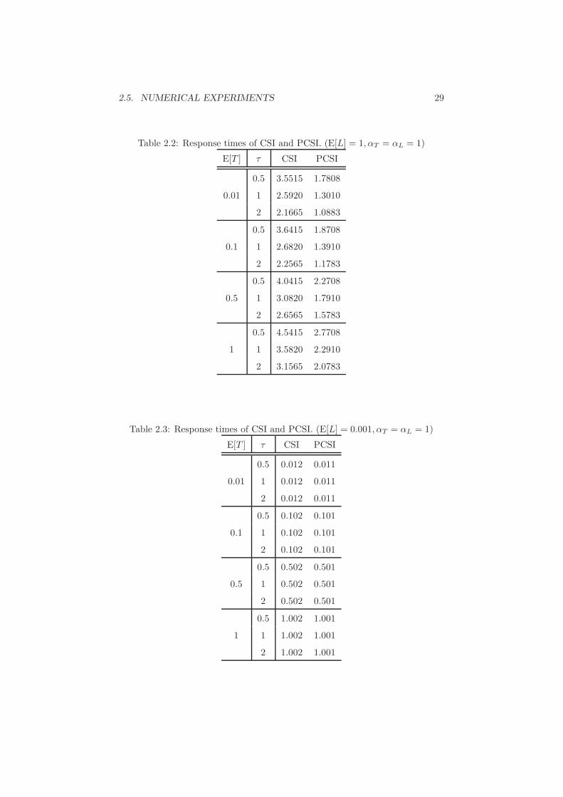
2.5.2 Response Time
We first investigate the impacts to response time of CSI and PCSI under failure-
prone environment. In the experiments, we fix the arrival rate of transaction
in the replica λR = 1, i.e., the inter-arrival time of transaction becomes 1.
We also set the arrival rate of transaction in the master λA = 1. Moreover,
for investigating the effect of restart scheme, we set the restart time limit in
three cases, τ = 0.5, 1, 2 and a fixed restart overhead time c = 0.5 constantly.
Table 2.1 presents the response times of CSI and PCSI where λA = 1, αT =
αL = 1, E[T ] = 0.01 and τ = 0.5. Note that the response times can be
calculated by Eq. (2.18) and (2.26). As same as the conclusion showed in [10,
18], it can be found from Table 2.1 that the PCSI is effective to reducing the
response time. Particularly in the case when latency is large, i.e., E[L] = 1, PCSI
provides about half the response time of CSI. Therefore, in order to examine
the impact caused by communication failures, we show the response times of
CSI and PCSI with fixing the mean time of communication latency E[L] = 1
and αT = αL = 1 in Table 2.2. From this table, it can be observed that
response times under both isolation policies reduce as the restart time limit τ
gets enlarged. In contract, Table 2.3 shows the response times when latency is
comparatively short, E[L] = 0.001. It is inferred that restart scheme reduces
system performance significantly when communication latency is too large to
be ignored. With considering the network environment, the usage of request
restart scheme is supposed be implemented in the database systems with small
communication delay. In addition, we inspect the effects from distribution of
latency time. Let αL, the shape parameter of latency time which is following
defective gamma distribution, equals 0.5, 1, 2, 5, respectively. Table 2.4 presents
the response times in a set of shape parameters of latency time distribution and
restart time limits. Notice that the response time of CSI while αL = 5 and
τ = 0.5 is much larger than other situations. Since the property of shape
parameter in gamma distribution, it can be supposed that the mean time of
latency stays steady when αL is less than 1, and stays variable when αL is
larger than 1. While αL = 5, the communication latency may values in wider
range, and it exactly represents different reasons by which the communication
delays caused.

28CHAPTER 2. PERFORMANCE EVALUATION OF SNAPSHOT ISOLATION
Table 2.1: Response times of CSI and PCSI. (τ = 0.5, αT = αL = 1)
E[T ] E[L] CSI PCSI
0.001 0.0120 0.0110
0.01 0.01 0.0300 0.0200
0.1 0.2168 0.1134
1 3.5515 1.7808
0.001 0.1020 0.1010
0.1 0.01 0.1200 0.1100
0.1 0.3068 0.2034
1 3.6415 1.8708
0.001 0.5020 0.5010
0.5 0.01 0.5200 0.5100
0.1 0.7068 0.6034
1 4.0415 2.2708
0.001 1.0020 1.0010
1 0.01 1.0200 1.0100
0.1 1.2068 1.1034
1 4.5415 2.7708
2.5. NUMERICAL EXPERIMENTS 29
Table 2.2: Response times of CSI and PCSI. (E[L] = 1, αT = αL = 1)
E[T ] τ CSI PCSI
0.5 3.5515 1.7808
0.01 1 2.5920 1.3010
2 2.1665 1.0883
0.5 3.6415 1.8708
0.1 1 2.6820 1.3910
2 2.2565 1.1783
0.5 4.0415 2.2708
0.5 1 3.0820 1.7910
2 2.6565 1.5783
0.5 4.5415 2.7708
1 1 3.5820 2.2910
2 3.1565 2.0783
Table 2.3: Response times of CSI and PCSI. (E[L] = 0.001, αT = αL = 1)
E[T ] τ CSI PCSI
0.5 0.012 0.011
0.01 1 0.012 0.011
2 0.012 0.011
0.5 0.102 0.101
0.1 1 0.102 0.101
2 0.102 0.101
0.5 0.502 0.501
0.5 1 0.502 0.501
2 0.502 0.501
0.5 1.002 1.001
1 1 1.002 1.001
2 1.002 1.001

30CHAPTER 2. PERFORMANCE EVALUATION OF SNAPSHOT ISOLATION
Table 2.4: Response times of CSI and PCSI. (E[L] = 1,E[T ] = 0.01, αT = 1)
αL τ CSI PCSI
0.5 2.1641 1.0871
0.5 1 1.9866 0.9983
2 1.9581 0.9841
0.5 3.5515 1.7808
1 1 2.5920 1.3010
2 2.1665 1.0883
0.5 6.1866 3.0983
2 1 3.1492 1.5796
2 2.1915 1.1007
0.5 17.1609 8.5855
5 1 3.7446 1.8773
2 2.0827 1.0464
2.5.3 System Throughput
Next we discuss the system performances of CSI and PCSI in terms of through-
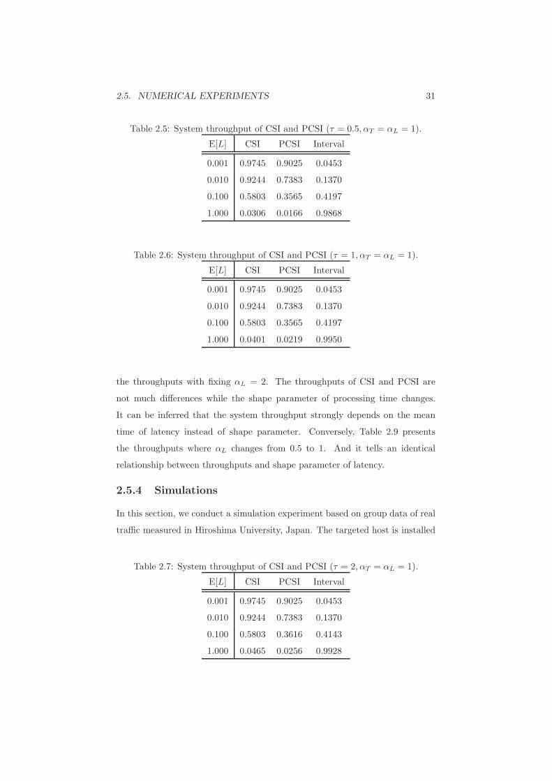
put. In Tables 2.5–2.7, where we set the restart time τ = 0.5, 1, 2 respectively,
the system throughputs of PCSI with optimized time interval show a decrease
comparing with that in CSI. In addition, PCSI with restart scheme performs
about 90% of CSI in term of throughput, when latency is contrastively small.
And the ratio between throughputs of PCSI and CSI, when E[L] = 1.0, is re-
duced to about 55%. It implies that if the network environment is crowded,
system has to pay more expense for ensuring successful communications. In
contrast, restart scheme is more effective under unblocked network condition.
On the other hand, the performances are almost equal for each restart time τ ,
except the high latency situation, i.e., E[L] = 1.0. It can be implied that the
restart time limit will affect the system performance more significantly when la-
tency is large. Thus, the trade-off of the system performance and the guarantee
of success communication should be considered especially in lagging network.
For inspecting the sensitivity of throughput to the distribution parameters,
we fix parameters as τ = 1, E[L] = 0.001, E[T ] = 0.01. Table 2.8 shows
2.5. NUMERICAL EXPERIMENTS 31
Table 2.5: System throughput of CSI and PCSI (τ = 0.5, αT = αL = 1).
E[L] CSI PCSI Interval
0.001 0.9745 0.9025 0.0453
0.010 0.9244 0.7383 0.1370
0.100 0.5803 0.3565 0.4197
1.000 0.0306 0.0166 0.9868
Table 2.6: System throughput of CSI and PCSI (τ = 1, αT = αL = 1).
E[L] CSI PCSI Interval
0.001 0.9745 0.9025 0.0453
0.010 0.9244 0.7383 0.1370
0.100 0.5803 0.3565 0.4197
1.000 0.0401 0.0219 0.9950
the throughputs with fixing αL = 2. The throughputs of CSI and PCSI are
not much differences while the shape parameter of processing time changes.
It can be inferred that the system throughput strongly depends on the mean
time of latency instead of shape parameter. Conversely, Table 2.9 presents
the throughputs where αL changes from 0.5 to 1. And it tells an identical
relationship between throughputs and shape parameter of latency.
2.5.4 Simulations
In this section, we conduct a simulation experiment based on group data of real
traffic measured in Hiroshima University, Japan. The targeted host is installed
Table 2.7: System throughput of CSI and PCSI (τ = 2, αT = αL = 1).
E[L] CSI PCSI Interval
0.001 0.9745 0.9025 0.0453
0.010 0.9244 0.7383 0.1370
0.100 0.5803 0.3616 0.4143
1.000 0.0465 0.0256 0.9928

32CHAPTER 2. PERFORMANCE EVALUATION OF SNAPSHOT ISOLATION
Table 2.8: System throughput of CSI and PCSI (αL = 2).
αT CSI PCSI Interval
0.5 0.9745 0.9018 0.0453
1.0 0.9745 0.9025 0.0454
2.0 0.9745 0.9029 0.0451
5.0 0.9744 0.9032 0.0447
Table 2.9: System throughput of CSI and PCSI (αT = 2).
αL CSI PCSI Interval
0.5 0.9745 0.9029 0.0450
1.0 0.9745 0.9029 0.0451
2.0 0.9745 0.9029 0.0451
5.0 0.9745 0.9029 0.0452
in the Department of Information Engineering in Hiroshima university. The
accessing records are collected for one day and the number of total records is
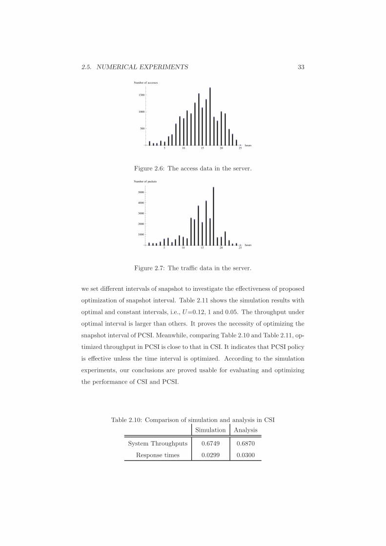
16529. We further aggregate the group data at 1 hour’s time interval so as
to summary the characteristic of arrival stream into parameters in Figure 2.6.
Also, by observing the traffic packets data in Figure 2.7, we can empirically
gain the density of traffic which can be applied as the parameters of processing
time. Then we set Monte Carlo simulations with the these system parameters
and survey the system throughputs and response times.
Next, we numerically calculate the throughput and response time by us-
ing our formulations. The mean time between arrivals 1/λA is 0.087 min and
the mean processing time E[T ] is 0.018 min. We assume the latency time
E[L] = 0.01, αT = αL = 1, c = 0.5 and τ = 0.5. Table 2.10 shows the
comparison of simulation and analysis results with CSI policy. The response
times are almost the same and the analytical throughput are close to that of
simulation. The correctness of our formulations can be validated. On the other
hand, we generate requests under PCSI policy by same parameters. Since the
time interval of snapshot is difficult to be determined by observed data, we
firstly use the optimal value obtained by proposed equations, U∗ = 0.12. Then,
2.5. NUMERICAL EXPERIMENTS 33
5 10 15 20 25hours
500
1000
1500
Number of accesses
Figure 2.6: The access data in the server.
5 10 15 20 25hours
1000
2000
3000
4000
5000
Number of packets
Figure 2.7: The traffic data in the server.
we set different intervals of snapshot to investigate the effectiveness of proposed
optimization of snapshot interval. Table 2.11 shows the simulation results with
optimal and constant intervals, i.e., U=0.12, 1 and 0.05. The throughput under
optimal interval is larger than others. It proves the necessity of optimizing the
snapshot interval of PCSI. Meanwhile, comparing Table 2.10 and Table 2.11, op-
timized throughput in PCSI is close to that in CSI. It indicates that PCSI policy
is effective unless the time interval is optimized. According to the simulation
experiments, our conclusions are proved usable for evaluating and optimizing
the performance of CSI and PCSI.
Table 2.10: Comparison of simulation and analysis in CSI
Simulation Analysis
System Throughputs 0.6749 0.6870
Response times 0.0299 0.0300

34CHAPTER 2. PERFORMANCE EVALUATION OF SNAPSHOT ISOLATION
Table 2.11: Comparison of simulation and analysis in PCSI
Simulation Analysis
Optimal U=1 U=0.05
System Throughputs 0.6358 0.0935 0.3796 0.6510
Response times 0.0278 0.0281 0.0280 0.0280

Chapter 3
Optimal Planning for OpenSource Software Updates
Optimal Planning for Open Source Software Updates
Open source software is widely deployed for both academic and commercial
proposes. However, failures and attacks against open source software are greatly
reported. Being different from traditional software, failures of open source soft-
ware are reported by users and fixed by developers. With the overheads and
costs of updates, users would not maintain the software immediately the latest
update is released. We are attracted by the optimal maintenance problem for
open source software from users’ perspective. In this chapter, we proposes pe-
riodic and aperiodic maintenance management models with non-homogeneous
bug-discovery/correction processes in terms of total expense. Also, according to
a dynamic programming algorithm, we numerically derive the optimal mainte-
nance schedule under aperiodic policy. In numerical examples, we investigate
the efficiency of proposed policies by mathematical experiments. And, based on
bug reports of Hadoop MapReduce, we predictively illustrate the optimal main-
tenance scheduling for a real open source software product.
3.1 Bug-Correction Process
We focus on the bug-discovery/correction process in the open source project.
In general, the open source project has no clear distinction between implement
and testing phases. If users discover yet-undetected bugs in using the software,
they report details of the bugs to the community of open source project and
35

36CHAPTER 3. OPTIMAL PLANNING FOROPEN SOURCE SOFTWARE UPDATES
developers start to fix the bugs. Thus the bug-discovery process seems to be evo-
lutionary, and it is different from the traditional software development process
such as waterfall model. However, if we focus on particular versions of the soft-
ware, it is known that the number of discovered bugs is able to be represented
by the traditional software reliability growth model (SRGM).
In this chapter, we generally apply the NHPP-based SRGM for character-
izing the bug-discovery phenomenon due to two reasons: 1) The effectiveness
of NHPP-based SRGMs are affirmed for describing the stochastic behavior of
the number of detected faults, because of their tractability and goodness-of-fit
performance. Also, dozens of NHPP-based SRGMs are proposed and improved
for fitting different software projects. [36, 53] 2) According to these models,
several software reliability assessment tools are developed for evaluating soft-
ware reliability and predicting the residual bugs. [48, 55] These tools make it
possible to find the best matching model for particular software product.
Also, as mentioned by Shibata, [61] the repair time for one bug is considered
as an exponential random variable. Thus, the generation of available patches is
governed as the output of an Mt/M/∞ queueing model. According to queueing
theory, the output stream is following a NHPP model if the arrival, i.e., the
discovery process, is also a NHPP.
In the software reliability engineering, the SRGM has been used to present
the behavior of the number of faults detected in testing phase. Generally, the
model is constructed under the following assumptions:
1. The software involves a fixed and finite number of faults before testing
and it is a Poisson random variable with mean ω.
2. The times to correct a fault are stochastic and mutually independent ran-
dom variables having the cumulative distribution function F (t).
According to the above assumption, the cumulative number of faults corrected
3.2. MAINTENANCE COST MODEL 37
before time t has the following probability mass function (p.m.f.):
P (B(t) = n) =
∞∑
m=n
P (B(t) = n|B(0) = m)P (B(0) = m)
=
∞∑
m=n
(
m
n
)
F (t)n(1− F (t))m−nωm
m!exp(−ω)
=(ωF (t))n
n!exp(−ωF (t)). (3.1)
The above p.m.f. is equivalent to the non-homogeneous Poisson process (NHPP)
with mean value function E[B(t)] = ωF (t).
When we focus on the particular versions of software, the above two assump-
tions are also plausible even in the open source software. Thus in this chapter,
we use the traditional SRGM to represent the bug-discovery process in the open
source project, i.e., the NHPP B(t) means the number of discovered bugs in the
particular versions of open source software. In fact, when F (t) is a truncated
logistic distribution, the corresponding NHPP model is called the inflection S-
shaped model whose mean value function draws a logistic curve. [44, 45] It has
been reported that the logistic curve fitted to the actual bug (vulnerability)
discovery process of open source software. [4, 3, 66, 2]
3.2 Maintenance Cost Model
In this chapter, we consider the maintenance model for the system whose in-
frastructure is constructed by open source software; for example, the virtual
environment is provided by Xen1 as infrastructure, some large-scale file systems
involve MapReduce2 as an important module, and even a simple Linux-based
system also relies on Linux kernel3. In such system, from the reliability and
security points of view, the infrastructure software should be kept to the latest
and stable version. Even if the infrastructure has a security hole, the system
may suffer malicious attacks and eventually happens the system or security fail-
ure such as system down, intrusion and falsification. On the other hand, during
the update of infrastructure, the system should be stopped. That is, there is a
trade-off relationship between failure and maintenance.
1http://www.xenproject.org/2http://hadoop.apache.org/3https://www.kernel.org/

38CHAPTER 3. OPTIMAL PLANNING FOROPEN SOURCE SOFTWARE UPDATES
Suppose that the open source software is continuously maintained in the
project. That is, if one reports a bug, developers immediately try to fix the bug.
Then the reliability growth of the particular versions of open source software is
given by an NHPP model described in the previous section. Let B(t) be the
cumulative number of corrected bugs and its p.m.f. is written by
P (B(t) = n) =(ωF (t))n
n!exp−ωF (t), n = 0, 1, . . . . (3.2)
Also we assume that the particular versions of open source software will be used
as infrastructure in the calendar time period [ts, te]. Note that the calendar
time starts at the time when the development of particular versions of software
begins. Without loss of generality, m updates are applied in the period [ts, te],
i.e., we define the time sequence of maintenance as ts = t0 < t1 < t2 < · · · <
tm < tm+1 = te. For notational convenience, t0 and tm+1 are equivalent to ts
and te respectively.
Here we focus on the number of residual bugs in the software. When the
number of corrected bugs B(t) is known, the number of residual bugs R(t) is
predicted by R(t) = B(∞)−B(t);
P (R(t) = n) =(ωF (t))n
n!exp(−ωF (t)), n = 0, 1, . . . (3.3)
where F (t) = 1−F (t). On the other hand, the number of residual bugs in user
environment can be decreased only at the time when the system is updated.
Figure 3.1 illustrates possible sample paths of the number of residual bugs in the
latest version of repository and in user environment. As shown in the figure, the
bugs corrected during [ti−1, ti] are fixed only at ti in user environment, although
the number of residual bugs in the latest version continuously decreases.
To build the cost model for maintenance, we define the following two cost
parameters:
• cm: The maintenance cost per software update.
• cf : The penalty/recovery cost per failure.
As mentioned before, the maintenance incurs some penalty cost while the system
is unavailable and the work cost for applying the update. The cost cm indicates
the total cost required for the system to undergo maintenance. When the system

3.3. OPTIMAL UPDATE SCHEDULING 39
is failed by the residual bugs, the cost cf is required to recovery the system
down, intrusion and falsification. For the sake of simplification, even if the
system failure is happened, the software update is not executed and the system
is recovered as the same version of software. Also, maintenance and recovery
time durations are negligible since time intervals of updates are relatively larger
than maintenance and recovery time durations.
Here we assume that the frequency of failure occurrences is proportional
to the number of residual bugs, i.e., the failure rate of software at time t is
given by λR(t), where λ is the parameter meaning the failure rate per bug. In
particular, it should be noted that the failure rate is piecewise constant at the
period [ti−1, ti] for each i = 1, . . . ,m in the user environment. Thus the expected
number of failures Xi at the i-th period [ti−1, ti] in the user environment is given
by
E[Xi] =
∞∑
n=0
E[Xi|R(ti−1) = n]P (R(ti−1) = n)
= (ti − ti−1)λE[R(ti−1)]
= (ti − ti−1)λωF (ti−1). (3.4)
Thus the expected total maintenance cost in the period [t0, tm+1] becomes
C(t1, . . . , tm; t0, tm+1) = cmm+
m+1∑
i=1
cfE[Xi]
= cmm+ cfλω
m+1∑
i=1
(ti − ti−1)F (ti−1). (3.5)
3.3 Optimal Update Scheduling
Based on the cost model, the problem is to find the optimal schedule for updates
minimizing the expected total maintenance cost;
(t∗1, . . . , t∗m) = argmin
(t1,...,tm)
C(t1, . . . , tm; t0, tm+1). (3.6)
Note that t0 and tm+1 are fixed. In the chapter, we discuss two different sched-
ules under respective constraints.

40CHAPTER 3. OPTIMAL PLANNING FOROPEN SOURCE SOFTWARE UPDATES
0
2
4
6
8
10
0
2
4
6
8
10
t0 t1 t2 t3 time
time
#ofre
sid
ualbugs
of
the
late
stvers
ion
#ofre
sid
ualbugs
in
user
environm
ent
R(t0)
R(t0)
R(t1)
R(t1)
R(t2)
R(t2)
R(t3)
R(t3)
Figure 3.1: Possible sample paths of the number of residual bugs.
3.3.1 Periodic Policy
The first policy is the periodic policy under which the time intervals of updates
are identical. In fact, the maintenance is performed every week, month or year
in many pragmatic systems. Let s be the time interval of updates. The expected
total cost can be rewritten by
C(s; ts, te) = cmh+ cfλωs
h−1∑
i=0
F (ts + is) + cfλω[(te − ts)− hs]F (ts + hs),
(3.7)
where h is the number of updates that is given by h = max{n is a non-negative integer; te−
ts > ns}. The last term corresponds to the penalty/recovery cost at the period
[hs, te] since the time interval of update is (te−ts)−hs. According to the above,
we find some properties of the optimal maintenance schedule. For example, if
the number of residual bugs does not decrease, namely F (t) = constant, in the
time period t ∈ [ts, te], then the optimal maintenance policy becomes the policy
under which the system update is never applied. The cost in this case is given
by
C(s; ts, te) = cf (te − ts)λωF (ts), for s ≥ te − ts. (3.8)

3.3. OPTIMAL UPDATE SCHEDULING 41
Since lims→0 C(s; ts, te) = +∞, Eq. (3.8) also gives the upper bound of the
minimum cost. On the other hand, the penalty/recovery cost depends on the
expected area of the number of residual bugs; E[∫ te
tsR(t)dt]. Then the lower
bound of minimum cost is given by
C(s; ts, te) ≥ cfλω
∫ te
ts
F (t)dt, for any s. (3.9)
From these results, we have
cfλω
∫ te
ts
F (t)dt ≤ C(s∗; ts, te) ≤ cf (te − ts)λωF (ts), (3.10)
where s∗ the optimal time interval minimizing Eq. (3.7).
3.3.2 Aperiodic Policy
The second is the aperiodic policy under which the time intervals of updates are
allowed to be different. If F (t) is constant, the system update is meaningless to
reduce the maintenance cost. On contrary, while the number of residual bugs
rapidly decreases, we intuitively knows that it is better to perform the system
updates frequently. That is, the appropriate time intervals of updates depend
on behavior of the number of residual bugs and are not constant. From this
insight, we consider the aperiodic policy to determine the optimal maintenance
schedule minimizing the maintenance cost.
First we consider the optimization problem when the number of updates in
[ts, te] is fixed as m. In Eq. (3.5), we find that the original problem can be
reduced to the optimization of the following equation:
mint1,...,tm
m+1∑
i=1
(ti − ti−1)F (ti−1). (3.11)
This implies that cost parameters do not affect the optimal maintenance sched-
ule when the number of updates is fixed. By taking the first derivatives of Eq.
(3.11) with respect to t1, . . . , tm, we obtain the optimality condition;
t∗i+1 − t∗i =F (t∗i−1)− F (t∗i )
f(t∗i+1), for i = 1, . . . ,m, (3.12)
where t∗0 = ts and t∗m+1 = te are fixed. Ideally, by solving the above non-linear
equations, we get the optimal maintenance schedule under the fixed number of
updates. However, it is not easy to compute it from the computational point of
view.
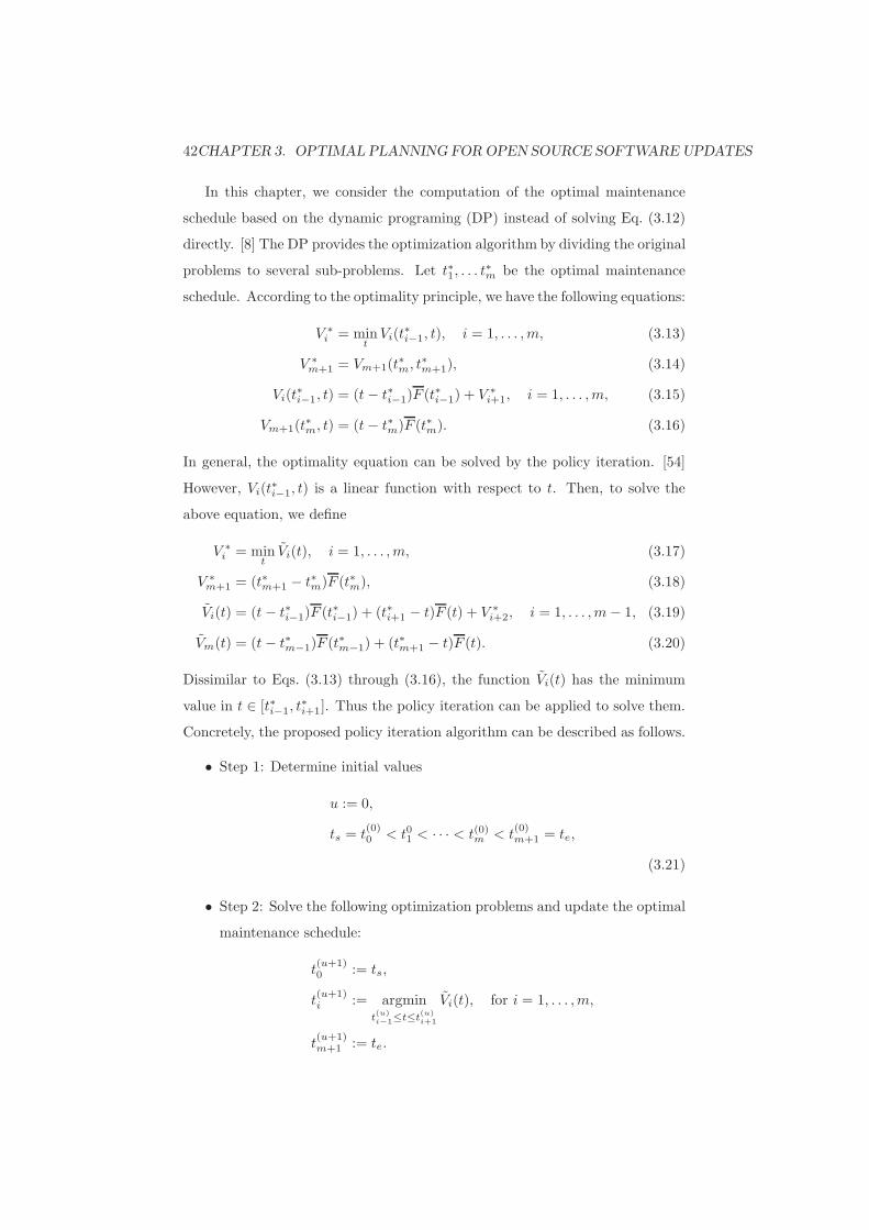
42CHAPTER 3. OPTIMAL PLANNING FOROPEN SOURCE SOFTWARE UPDATES
In this chapter, we consider the computation of the optimal maintenance
schedule based on the dynamic programing (DP) instead of solving Eq. (3.12)
directly. [8] The DP provides the optimization algorithm by dividing the original
problems to several sub-problems. Let t∗1, . . . t∗m be the optimal maintenance
schedule. According to the optimality principle, we have the following equations:
V ∗i = mint
Vi(t∗i−1, t), i = 1, . . . ,m, (3.13)
V ∗m+1 = Vm+1(t∗m, t∗m+1), (3.14)
Vi(t∗i−1, t) = (t− t∗i−1)F (t∗i−1) + V ∗i+1, i = 1, . . . ,m, (3.15)
Vm+1(t∗m, t) = (t− t∗m)F (t∗m). (3.16)
In general, the optimality equation can be solved by the policy iteration. [54]
However, Vi(t∗i−1, t) is a linear function with respect to t. Then, to solve the
above equation, we define
V ∗i = mint
Vi(t), i = 1, . . . ,m, (3.17)
V ∗m+1 = (t∗m+1 − t∗m)F (t∗m), (3.18)
Vi(t) = (t− t∗i−1)F (t∗i−1) + (t∗i+1 − t)F (t) + V ∗i+2, i = 1, . . . ,m− 1, (3.19)
Vm(t) = (t− t∗m−1)F (t∗m−1) + (t∗m+1 − t)F (t). (3.20)
Dissimilar to Eqs. (3.13) through (3.16), the function Vi(t) has the minimum
value in t ∈ [t∗i−1, t∗i+1]. Thus the policy iteration can be applied to solve them.
Concretely, the proposed policy iteration algorithm can be described as follows.
• Step 1: Determine initial values
u := 0,
ts = t(0)0 < t01 < · · · < t(0)m < t
(0)m+1 = te,
(3.21)
• Step 2: Solve the following optimization problems and update the optimal
maintenance schedule:
t(u+1)0 := ts,
t(u+1)i := argmin
t(u)i−1≤t≤t
(u)i+1
Vi(t), for i = 1, . . . ,m,
t(u+1)m+1 := te.

3.4. NUMERICAL EXAMPLES 43
• Step 3: For all i = 1, . . . ,m, if |t(u+1)i − t
(u)i | < δ, stop the algorithm,
where δ is an error tolerance level. Otherwise, let u := u + 1 and go to
Step 2.
In Step 2, an arbitrary optimization technique should be applied. Since Vi(t)
has the minimum value in the range [ti−1, ti+1], it is not difficult to find it. For
instance, the golden section method would be effective to find the solution. [26]
Next we consider the optimal number of updates m∗. The problem can be
formulated as follows.
minm
(cmm+ cfλωS∗(m)) , (3.22)
where
S∗(m) = mint1,...,tm
m+1∑
i=1
(ti − ti−1)F (ti−1). (3.23)
Note that S∗(m) depends on the optimal maintenance schedule.
Suppose that the cost for update is positive, i.e., cm > 0. Then the main-
tenance cost infinitely increases as m increases, since the expected total failure
cost has the lower bound shown in the previous section. Thus it is easy to
see that the optimal number of updates exists in finite domain; 0 ≤ m∗ < ∞.
Moreover, Eq. (3.23) is a monotonically decreasing function of m and cmm is
linearly increasing with respect to m. Then we find the optimal number of
updates satisfying
m∗ = min{m ≥ 0; cm + cfλω(S∗(m)− S∗(m− 1)) > 0}. (3.24)
3.4 Numerical Examples
3.4.1 Characteristic Analysis
We first investigate the characteristics of periodic and aperiodic maintenance
policies by numerical experiments. As mentioned before, the cost parameters
have no effect to the optimal maintenance schedule under a fixed number of
m. Without considering the cost parameters, we first define two mean value
functions for a bug-correction process:
R(t) = ω(1− e−at) (3.25)
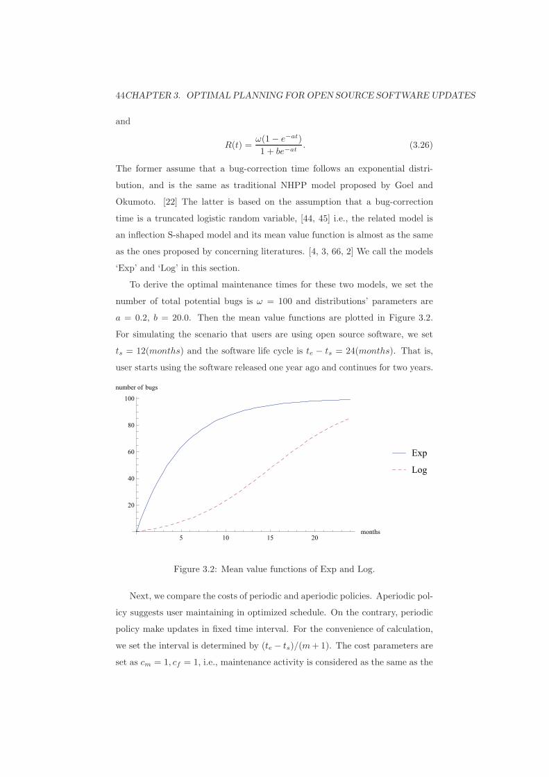
44CHAPTER 3. OPTIMAL PLANNING FOROPEN SOURCE SOFTWARE UPDATES
and
R(t) =ω(1− e−at)
1 + be−at. (3.26)
The former assume that a bug-correction time follows an exponential distri-
bution, and is the same as traditional NHPP model proposed by Goel and
Okumoto. [22] The latter is based on the assumption that a bug-correction
time is a truncated logistic random variable, [44, 45] i.e., the related model is
an inflection S-shaped model and its mean value function is almost as the same
as the ones proposed by concerning literatures. [4, 3, 66, 2] We call the models
‘Exp’ and ‘Log’ in this section.
To derive the optimal maintenance times for these two models, we set the
number of total potential bugs is ω = 100 and distributions’ parameters are
a = 0.2, b = 20.0. Then the mean value functions are plotted in Figure 3.2.
For simulating the scenario that users are using open source software, we set
ts = 12(months) and the software life cycle is te − ts = 24(months). That is,
user starts using the software released one year ago and continues for two years.
5 10 15 20months
20
40
60
80
100
number of bugs
Exp
Log
Figure 3.2: Mean value functions of Exp and Log.
Next, we compare the costs of periodic and aperiodic policies. Aperiodic pol-
icy suggests user maintaining in optimized schedule. On the contrary, periodic
policy make updates in fixed time interval. For the convenience of calculation,
we set the interval is determined by (te − ts)/(m+ 1). The cost parameters are
set as cm = 1, cf = 1, i.e., maintenance activity is considered as the same as the
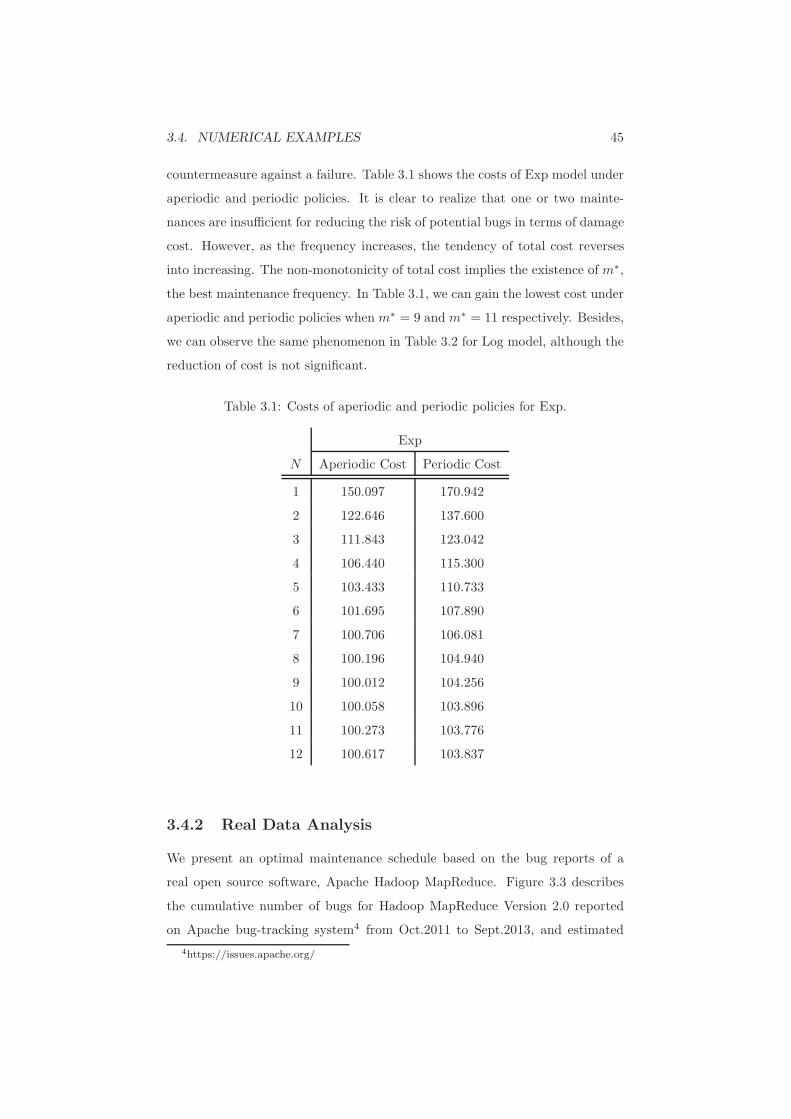
3.4. NUMERICAL EXAMPLES 45
countermeasure against a failure. Table 3.1 shows the costs of Exp model under
aperiodic and periodic policies. It is clear to realize that one or two mainte-
nances are insufficient for reducing the risk of potential bugs in terms of damage
cost. However, as the frequency increases, the tendency of total cost reverses
into increasing. The non-monotonicity of total cost implies the existence of m∗,
the best maintenance frequency. In Table 3.1, we can gain the lowest cost under
aperiodic and periodic policies when m∗ = 9 and m∗ = 11 respectively. Besides,
we can observe the same phenomenon in Table 3.2 for Log model, although the
reduction of cost is not significant.
Table 3.1: Costs of aperiodic and periodic policies for Exp.
Exp
N Aperiodic Cost Periodic Cost
1 150.097 170.942
2 122.646 137.600
3 111.843 123.042
4 106.440 115.300
5 103.433 110.733
6 101.695 107.890
7 100.706 106.081
8 100.196 104.940
9 100.012 104.256
10 100.058 103.896
11 100.273 103.776
12 100.617 103.837
3.4.2 Real Data Analysis
We present an optimal maintenance schedule based on the bug reports of a
real open source software, Apache Hadoop MapReduce. Figure 3.3 describes
the cumulative number of bugs for Hadoop MapReduce Version 2.0 reported
on Apache bug-tracking system4 from Oct.2011 to Sept.2013, and estimated
4https://issues.apache.org/

46CHAPTER 3. OPTIMAL PLANNING FOROPEN SOURCE SOFTWARE UPDATES
Table 3.2: Costs of aperiodic and periodic policies for Log.
Log
N Aperiodic Cost Periodic Cost
1 183.952 187.768
2 158.500 162.044
3 147.566 150.629
4 141.792 144.433
5 138.433 140.736
6 136.394 138.431
7 135.155 136.978
8 134.438 136.086
9 134.079 135.583
10 133.978 135.359
11 134.066 135.343
12 134.153 135.476
mean value functions of bug-discovery models. Here we applied an estimation
method proposed by Okamura et al. to figure out the most fitting NHPP-based
SRM. [48] The bug-discovery model is approximately estimated as a truncated
extreme-value maximum (TEVM) distribution, whose mean value function is
given by
R(t) = ωΛ(t)− Λ(0)
1− Λ(0), (3.27)
Λ(t) = exp(− exp(−t− b
a)), (3.28)
where a and b are parameters of TEVM distribution respectively. The parameter
estimation for all the models involved by Okamura et al. is based on maximum
likelihood estimation (MLE). [48] The estimated parameters for TEVM model
are described in Table 3.3. This table also presents the corresponding maximum
logarithmic likelihood (MLL) and Akaike’s information criterion (AIC). Com-
monly the AIC is used as an information criterion to assess the goodness-of-fit
between data and model. The model with a smaller AIC is better fitted to data.
From this argument, it can be indicated that TEVM model is better fitted to

3.4. NUMERICAL EXAMPLES 47
the bug data for Hadoop MapReduce than the others. In addition, the mean
value function in Fig. 3.3 predictively shows number of found bugs from Oct.
2013 for about one more year.
Figure 3.3: Hadoop: bug data and estimated mean value functions.
Table 3.3: Estimation results for bug data.
Model MLL AIC Parameters
Truncated Extreme-Value Maximum -268.66 543.32 ω = 389.02,
α = 193.92,
β = 382.67.
Next we perform the proposed maintenance policies with the estimated mean
value function of TEVM model which is supposed as the best fitting model
in terms of AIC in the next year. We initially investigate the time intervals
between two updates under periodic and aperiodic policies. Assume user start
using Hadoop MapReduce after two years, ts = 730 and the life period of the

48CHAPTER 3. OPTIMAL PLANNING FOROPEN SOURCE SOFTWARE UPDATES
software is one year, i.e. te − ts = 365, and the first application of Hadoop
MapReduce starts at Oct. 2013, Then the total number of updates during the
software life period is given by m = 12. We use the estimated parameters of
TEVM model to predict the residual bugs of software. Figure 3.4 illustrates
the time intervals of updates under two policies when m = 12. The intervals of
aperiodic policy are not constant strictly, and the intervals at the ending part
become longer than the ones at the beginning.
Figure 3.4: Time intervals of updating times (m = 12).
We also exam the determination of total update times, m∗. By setting the
cost parameters as cm = 1, cf = 1, and the constant bug rate λ = 0.004, we
obtain Figure 3.5. This figure numerically shows the existence of m∗ under
both aperiodic and periodic polices. From the parameters setting, we may tell a
scenario; if the costs of repairing a failure and applying a update are identical,
user should update the software 6 times for gaining the least cost.
With the above parameters, we further investigate the effectiveness of opti-
mization of m. The optimized cost under aperiodic policy and the costs with
different m are shown in Table 3.4. Under periodic policy, user update patches

3.4. NUMERICAL EXAMPLES 49
in fixed interval, which are set as half a year, two months, one month and two
weeks. Since the life period is given by a constant, the total numbers of update
are fixed as 1, 5, 11 and 25. Comparing these values with the cost when the
number of updates is optimized, we can see that the costs of periodic policy
are much higher than the aperiodic one, unless m = 5. It can be imply that
our proposal is useful to reduce the total cost. Also, by deriving m∗, redundant
updates can be averted. In practice, the available updates are not released as
frequent as one per two weeks. The result shows a practical significance for
maintenance scheduling.
Based on these numerical results, we can imply that aperiodic policy provides
more efficient maintenance plan while users update the software frequently or
infrequently. However, the periodic policy performs almost identically when
users apply the patches the same times as aperiodic policy. Thus, we can suggest
for the users of MapReduce module that the total number of patches should be
determined first. After that, the detailed patch timing can be decided equally
during the time span of usage. On the other hand, considering the characteristic
of software, we can see that the MapReduce module is used after sufficient
testing. That means residual bugs are few. In this situation, the periodic policy
is suitable for maintenance scheduling. If users begin to use a software product
without enough testing, the aperiodic policy should be strongly recommended
from the economic point of view.
Table 3.4: Total costs for aperiodic and periodic maintenance scheduling.
m∗ Aperiodic m Periodic
1 66.897(180-days)
5 54.0655(60-days) 5 55.6854(60-days)
11 58.2553(30-days)
25 70.4708(14-days)
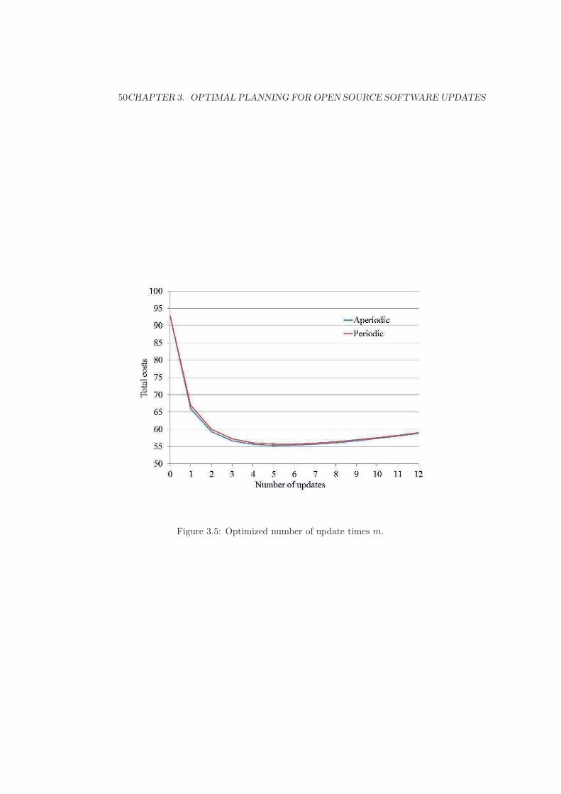
50CHAPTER 3. OPTIMAL PLANNING FOROPEN SOURCE SOFTWARE UPDATES
Figure 3.5: Optimized number of update times m.

Chapter 4
Quantifying Resiliency ofVirtualized System withSoftware Rejuvenation
This chapter considers how to evaluate the resiliency for virtualized system with
software rejuvenation. The software rejuvenation is a proactive technique to
prevent the failure caused by aging phenomenon such as resource exhaustion. In
particular, according to Gohsh et al. (2010), we compute a quantitative crite-
rion to evaluate resiliency of system by using continuous-time Markov chains
(CTMC). In addition, in order to convert general state-based models to CTMCs,
we employ PH (phase-type) expansion technique. In numerical examples, we in-
vestigate the resiliency of virtualized system with software rejuvenation under
two different rejuvenation policies.
4.1 Virtualized System with Software Rejuve-
nation
Consider the virtualized system with software rejuvenation proposed in [37,
38]. The system consists of virtual machines (VMs) and a virtual machine
monitor (VMM). The virtual machines provide services for the end users. In
general, VMs are used for Internet servers such as Web, mail and DB. Thus
the availability of VMs is important for quality of services. On the other hand,
VMM manages VMs in a physical machine. If VMM was stopped, all the VMs
on VMM should be stopped. Therefore it is important to decide optimal timings
51

52CHAPTER 4. QUANTIFYING RESILIENCYOFVIRTUALIZED SYSTEM
for triggering software rejuvenations for VM and VMM.
Machida et al. [37, 38] discussed three kinds of software rejuvenation policies
in such virtualized system; cold-VM, warm-VM and migrate-VM rejuvenations.
The cold-VM rejuvenation is the simplest rejuvenation. In the cold-VM rejuve-
nation, all the VMs running on the VMM are shut down before the rejuvenation
for VMM is performed. That is, although both VM and VMM are rejuvenated
by this operation, the time to shut down all the VMs is required. In addition,
the jobs running on VMs should be stopped or canceled before all the VMs are
shut down. The warm-VM rejuvenation is also called as the fast rejuvenation
[32]. In the warm-VM rejuvenation, instead of shutting down all the VM hosts,
they are resumed after the VMM rejuvenation and suspended before it. Since
the jobs running on the VMs are stored on memory, jobs are not canceled by
the rejuvenation though the job completion time becomes longer. Also, the
downtime is shorter than the cold-VM rejuvenation, because the time to wake
up from suspend mode is faster than boot time generally. The third rejuve-
nation is the migrate-VM rejuvenation. This scheme requires another VMM
which has the same environment as the original VMM. The live migration is
a well-known and convenient function of virtualized system, which can move
running VMs from one VMM to another VMM without downtime of service.
The migrate-VM rejuvenation utilizes the live migration of virtualized system.
That is, running VMs on one VMM are moved onto another VMM before the
VMM rejuvenation. After completion of the VMM rejuvenation, the migrated
VMs are back to the rejuvenated VMM. Although the jobs running on VMs
are never canceled by the warm-VM and migrate-VM rejuvenations, the soft-
ware aging of VMs is not rejuvenated by both the warm-VM and migrate-VM
rejuvenations. In this chapter, we consider the situation where a single VMM
is available such as private clouds. Since the migrate-VM rejuvenation requires
two or more VMMs as stand-by system. The chapter focuses on only cold-VM
and warm-VM rejuvenations, which are easily implemented even in a private
cloud environment.

4.2. MRSPN-BASED ANALYSIS 53
(a) VMM model
Phclock
PhpolicyPhtrigger
[ghpolicy]
Thpolicy
[ghreset]
Threset[ghinterval]
Thinterval
(b) VMM clock model
Figure 4.1: Part 1 of MRSPNs for the cold-VM rejuvenation [37, 38].
4.2 MRSPN-based Analysis
4.2.1 MRSPN Modeling
Markov regenerative stochastic Petri nets (MRSPNs) are one of the versatile
tools for model-based performance evaluation [16, 20], which is extensions of
generalized stochastic Petri nets (GSPNs). MRSPN can deal with GEN tran-
sitions whose firing time follows a general distribution, while GSPN consists of
only immediate transitions and EXP transitions whose firing time follows an
exponential distribution. Thus MRSPNs have high representation ability for
stochastic modeling, and in fact, many application models arising in computer
communication systems can be described by MRSPNs [17, 34].
(i) MRSPN for Cold-VM Rejuvenation:
Figure 4.1 and 4.2 illustrate MRSPN representation for the cold-VM rejuve-

54CHAPTER 4. QUANTIFYING RESILIENCYOFVIRTUALIZED SYSTEM
nation presented in [37, 38]. The model is divided into four layered MRSPNs.
The MRSPN (a) indicates the behavior of VMM under the cold-VM rejuvena-
tion. Each places represent the state of VMM;
• Phup: VMM is in the normal state.
• Phfp: VMM is in the failure-probable state, namely, VMM is degraded by
aging-related bugs.
• Phfail: VMM has been failed (failure state).
• Phdet: The failure has been detected and the repair operation is started
(repair state).
• Phrej : The rejuvenation operation is executed (rejuvenation state).
Also, each transition presents the event that occurs in VMM;
• Thfp: VMM becomes the failure-probable state.
• Threjt, Thfprejt: The rejuvenation operation for VMM is started.
• Threj: The rejuvenation operation is completed.
• Thfail: The failure occurs in VMM.
• Thdet: The failure has been detected and the repair operation is started.
• Threpair: The repair operation is completed.
The MRSPN (b) indicates the behavior of VMM rejuvenation policy. It is
managed by time-triggered policy, namely, the rejuvenation is triggered by a
periodic time which is represented by a GEN transition (black bar). Tghinterval
is enabled when a token is deposited in Phup or Phfp. The places Phpolicy means
that VMM is ready to execute rejuvenation operation. When the guards [ghpol-
icy] is satisfied, the tokens move to Phtrigger and start the rejuvenation. When
the VMM rejuvenation finishes, the immediate transition Threset is enabled and
a token is moved to Phclock. In MRSPN (a), the transitions Threjt and Thfprejt
fire when tokens are moved into Phtrigger . Once the rejuvenation operation is
started, the time counter of rejuvenation resets.

4.2. MRSPN-BASED ANALYSIS 55
Similar to the MRSPN (a) and (b), MRSPN (c) and (d) model the behaviors
of VM and VM rejuvenation policy under the cold-VM rejuvenation. The places
Pvup, Pvfp, Pvfail, Pvdet, Pvrej correspond to the state; normal, failure-probable,
failure, repair and rejuvenation states of VM. Also Pvsd and Pvfpsd represent
that the VM is shut down due to the VMM rejuvenation. The place Pvstop
means that the VM is stopped by a failure of VMM or VMM rejuvenation. The
transitions Tvfp, Tvrejt, Tvfprejt, Tvrej , Tvfail, Tvdet and Tvrepair are similar to
the events in VMM. On the other hand, Tvpre and Tvfppre indicate the preventive
shutdown for VM. The transition Tvdw is the event where VM is stopped due
to the VMM failure. Also, Tvsd and Tvfpsd are the completion of shutdown and
Tvrestart means the completion of restart of VM.
Cold-VM rejuvenation makes the hosted VM shut down before triggering
VMM rejuvenation. This policy is represented in the guard functions for the
immediate transitions Tvpre and Tvfppre. Either Tvpre or Tvfppre are enabled
when a token is deposited in Phpolicy in the VMM clock model. Then a token
is moved into Pvsd or Pvfpsd in the VM model. When a token is deposited in
Pvstop by firing Tvsd or Tvfpsd, the immediate transition Thpolicy is enabled by
[ghpolicy] and a VMM rejuvenation process starts. This ensures that VMM
rejuvenation does not start until the hosted VM is shut down properly. As in
the definition of [ghpolicy], we assume that VMM rejuvenation can start only
when a token is deposited in Pvstop, Pvfail, Pvdet or Pvrej .
(ii) MRSPN for Warm-VM Rejuvenation:
Figure 4.3 presents MRSPN for the behavior of VM under the warm-VM
rejuvenation [37, 38]. In the warm-VM rejuvenation, VM goes to suspend mode
before executing the VMM rejuvenation. Thus only the behavior of VM in the
warm-VM rejuvenation is different from the behavior of VM in the cold-VM re-
juvenation. The guard function [gvinterval] is modified to enable Tvinterval even
while a VM is in suspended state (a token is deposited in Pvsusd or Pvfpsusd).
The clock for VM rejuvenation is not affected by VM suspension. The guard
function [ghpolicy] enables Thpolicy only when a token is deposited in Pvsusd,
Pvfpsusd, Pvfail, Pvdet or Pvrej .
Warm-VM rejuvenation uses the suspend operation to stop the execution of
VM at VMM rejuvenation. This policy is represented in the guard functions
56CHAPTER 4. QUANTIFYING RESILIENCYOFVIRTUALIZED SYSTEM
for the immediate transitions Tvpre and Tvfppre. One of the two immediate
transitions Tvpre or Tvfppre is enabled when a token is deposited in Phpolicy in
the VMM clock model. When a token is deposited in Pvsusd or Pvfpsusd by
firing Tvsus or Tvfpsus, the VMM rejuvenation can start. One of the imme-
diate transitions Tvpost or Tvfppost is enabled, when the VMM rejuvenation is
completed and a token is deposited in Phup in the VMM model. The hosted
VM resumes the execution when a token is deposited in Pvup or Pvfp by the
transitions Tvresm or Tvfpresm. As defined in [ghpolicy], the VMM rejuvenation
can start only when a token is deposited in Pvsusd, Pvfpsusd, Pvfail, Pvdet or
Pvrej .
4.2.2 Transient Analysis
In [37, 38], Machida et al. derived the steady-state availability of the virtualized
system under the cold-VM and warm-VM rejuvenation based on the MRSPN
models. On the other hand, Okamura et al. [49] performed the transient analysis
for the virtualized system with cold-VM and warm-VM rejuvenation. Since
the resiliency analysis requires the transient analysis, we describe the transient
analysis of MRSPN.
The analysis begins with building MRGP (Markov regenerative process)
from the MRSPN. MRGP is a stochastic point process which has both regen-
erative and non-regenerative time points. Generally, we consider a stochastic
process {M(t); t ≥ 0} with discrete state space. If M(t) has time points at
which the process probabilistically restarts itself, the process is called regener-
ative, and the time points are called regeneration points. Otherwise, the time
points when M(t) does not restart are called non-regeneration points. Specifi-
cally, when state transition at the regeneration points is governed by a discrete
Markov chain (DTMC), the process M(t) is an MRGP. There are several meth-
ods for the transient analysis of MRGP such as the supplementary variable
(SV) method and discretization approach [20, 64]. In this chapter, we apply the
phase-type (PH) expansion to analyze MRGP.
The fundamental idea of PH expansion is to replace general distributions
in MRGP with approximate PH distributions, and it can reduce the original
MRGP to an approximate CTMC. The PH distribution is defined by the distri-
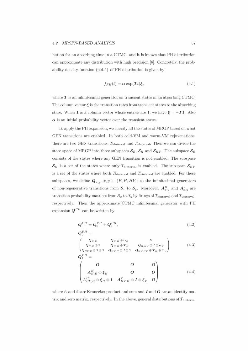
4.2. MRSPN-BASED ANALYSIS 57
bution for an absorbing time in a CTMC, and it is known that PH distribution
can approximate any distribution with high precision [6]. Concretely, the prob-
ability density function (p.d.f.) of PH distribution is given by
fPH(t) = α exp(T t)ξ, (4.1)
where T is an infinitesimal generator on transient states in an absorbing CTMC.
The column vector ξ is the transition rates from transient states to the absorbing
state. When 1 is a column vector whose entries are 1, we have ξ = −T1. Also
α is an initial probability vector over the transient states.
To apply the PH expansion, we classify all the states of MRGP based on what
GEN transitions are enabled. In both cold-VM and warm-VM rejuvenations,
there are two GEN transitions; Thinterval and Tvinterval. Then we can divide the
state space of MRGP into three subspaces SE , SH and SHV . The subspace SE
consists of the states where any GEN transition is not enabled. The subspace
SH is a set of the states where only Thinterval is enabled. The subspace SHV
is a set of the states where both Thinterval and Tvinterval are enabled. For these
subspaces, we define Qx,y, x, y ∈ {E,H,HV } as the infinitesimal generators
of non-regenerative transitions from Sx to Sy. Moreover, AHx,y and AV
x,y are
transition probability matrices from Sx to Sy by firings of Thinterval and Tvinterval,
respectively. Then the approximate CTMC infinitesimal generator with PH
expansion QPH can be written by
QPH = QPH0 +QPH
1 , (4.2)
QPH0 =
QE,E QE,H ⊗ αH O
QH,E ⊗ 1 QH,H ⊕ TH QH,HV ⊗ I ⊗ αV
QHV,E ⊗ 1⊗ 1 QHV,H ⊗ I ⊗ 1 QHV,HV ⊕ TH ⊕ TV
(4.3)
QPH1 =
O O O
AHH,E ⊗ ξH O O
AHHV,E ⊗ ξH ⊗ 1 AV
HV,H ⊗ I ⊗ ξV O
(4.4)
where ⊗ and ⊕ are Kronecker product and sum and I and O are an identity ma-
trix and zero matrix, respectively. In the above, general distributions of Thinterval

58CHAPTER 4. QUANTIFYING RESILIENCYOFVIRTUALIZED SYSTEM
and Tvinterval are approximately given by the following PH distributions:
fhinterval(t) ≈ αH exp(THt)ξH , (4.5)
fvinterval(t) ≈ αV exp(T V t)ξV . (4.6)
Then the approximate transient probabilities can be computed by the ordinary
transient analysis of CTMC with the approximate infinitesimal generator QPH .
Furthermore, there are several techniques to obtain the PH distribution
which approximates a general distribution. In this chapter, we use the EM-
based maximum likelihood estimation (see Appendix).
4.3 Quantification of System Resiliency
In this section, we introduce the quantitative measure for evaluating system
resiliency based on CTMC model. As mentioned before, the resiliency is one
of the effects of system indices when a change happens. According to [21],
we evaluate the resiliency of virtualized system with rejuvenation based on the
CTMC model in the following steps:
• Step 1: Compute the state probability vector and availability in the
steady-state.
• Step 2: Generate the infinitesimal generator when the change is applied.
• Step 3: Compute the transient behavior of availability after the change
by using the infinitesimal generator of Step 2 where the initial probability
vector is the steady state probability vector in Step 1.
In [21], settling time, peak overshoot or undershoot, peak time and γ-percentile
time are computed from the transient behavior. This chapter computes the
amount of deviation of measure which is defined by the area of difference be-
tween the steady-state measure and the deviation of measure by the change.
Concretely, let QN and QC be infinitesimal generators of system behavior dur-
ing normal and change conditions. Without loss of generality, the change is
applied in the period from t = 0 to t = Te. Also it is assumed that the measure
of interest is given by a dot product of the state probability vector π and a
reward vector (column vector) r, namely, πr. In the chapter, since we consider

4.4. EXPERIMENT 59
the availability as a measure of interest, the elements of reward vector are 0 or
1. If the system is available at a state, the reward of the state is 1. Otherwise,
if the system is unavailable at a state, the reward is 0.
The steady-state probability vector πs in the normal condition can be ob-
tained from the following equations:
πsQN = 0, πs1 = 1. (4.7)
By considering the state probability vector at any time can be represented by
the matrix exponential of infinitesimal generator, the amount of deviation of
measure (AD) is given by
AD =
∫ Te
0
|πsr − πs exp(QCt)r| dt
+
∫ ∞
0
|πsr − πs exp(QCTe) exp(QN t)r| dt. (4.8)
Figure 4.4 illustrates an example of the amount of deviation of measure. The
area in the figure corresponds to the amount of deviation of measure. If the
following equations hold for any t ≥ 0:
πsr > πs exp(QCt)r, (4.9)
πsr > πs exp(QCTe) exp(QN t)r, (4.10)
then Eq. (4.8) can be simplified to
AD =πsrTe − πs
∫ Te
0
exp(QCt)dtr
+ (πs − πs exp(QCTe))
∫ ∞
0
exp(QN t)dtr, (4.11)
where we use πs exp(QN t) = πs. In the above, we can apply the technique of
cumulative measures [57] to the integrals of matrix exponentials.
4.4 Experiment
In the experiment, we investigate the amount of deviation of system availability
when a change is applied. The model parameters are set as Table 4.1 which
are also used in [37, 38]. Also VM and VMM rejuvenations are triggered by
random variables. Due to the operating situation, VM and VMM rejuvenations
may be practically varied. VM rejuvenation is periodically performed at time

60CHAPTER 4. QUANTIFYING RESILIENCYOFVIRTUALIZED SYSTEM
Table 4.1: Model parameters in the experiment.
Transition Mean Time
Thfp 1 month
Thfail 1 week
Thdet 5 minutes
Threpair 1 hour
Threju 2 minutes
Tvfp 1 week
Tvfail 3 days
Tvdet 5 minutes
Tvrepair 30 minutes
Tvreju 1 minute
Tvsd, Tvfpsd 30 seconds
Tvrestart 30 seconds
Tvsus, Tvfpsus 0.08 seconds
Tvresm, Tvfpresm 0.8 seconds
interval which follows the normal distribution with mean 0.5, 1, 2 or 7 days,
and their coefficients of variation are fixed as 0.5. Similarly, VMM rejuvenation
is periodically performed at time interval which follows the normal distribution
with mean 7 (days) and the coefficient of variation 0.1. These normal distri-
butions are approximated by PH distributions with 50 phases by applying EM
algorithm [46] (see Appendix). Furthermore, we consider the following change
condition:
• The mean time of VM failure after aging is changed to 1/60 (hrs).
In this case, the change causes the degradation of availability. Then we can
use the formula of Eq. (4.11). Also we set the time duration of change as
Te = 5, 30, 60 minutes.
First we investigate the steady-state availabilities when the change contin-
ues, i.e., Te → ∞. Table 4.2 shows the steady-state availabilities when the
rejuvenation periods in cold-Vm and warm-VM rejuvenations are 0.5, 1, 2 and
7 days. The columns ‘Normal’ mean the steady-state availabilities under the

4.4. EXPERIMENT 61
Table 4.2: The steady-state availabilities in normal and change conditions.
Rejuvenation Cold-VM Warm-VM
interval Normal Change Normal Change
0.5 days 0.9948 0.9917 0.9976 0.9946
1 days 0.9970 0.9940 0.9980 0.9952
2 days 0.9978 0.9951 0.9979 0.9956
7 days 0.9975 0.9956 0.9972 0.9958
normal condition, and the columns ‘Change’ indicate the steady-state avail-
abilities under the change condition. From this table, we can see that there
is no remarkable difference between normal and change conditions in terms of
steady-state availabilities even though the failure rate in failure-probable state
drastically increases in the change condition. This is because the aging phe-
nomenon rarely occurs because of the software rejuvenation. In the table, the
change does not affect the steady-state availability strongly, and thus the effect
of change condition is not clear in terms of steady-state availability.
Next we investigate the system resiliency against the change. Figures 4.5, 4.6
and 4.7 illustrate the behavior of availabilities after the change is applied. In the
figures, the arrow indicates the time duration of change. Also cold(0.5), cold(1),
cold(2) and cold(7) mean the availabilities under the cold-VM rejuvenation.
The number in the bracket indicates the time interval of rejuvenation for VM,
i.e., 0.5, 1, 2 and 7 days time intervals of rejuvenation. Similarly, warm(0.5),
warm(1), warm(2) and warm(7) are the availabilities under the warm-VM re-
juvenation. For all the cases, the availability decreases by applying the change.
However, the speeds to go back to the steady state depend on the rejuvenation
policies. As the rejuvenation interval is small, the speed to go back to the steady
state becomes faster. Also by comparing the cold-VM and warm-VM rejuvena-
tions, we find the effect of change in the cold-VM rejuvenation is smaller than
that in the warm-VM rejuvenation.
Tables 4.3 and 4.4 present the amount of deviation of availability under the
cold-VM and warm-VM rejuvenations, respectively. From these tables, we con-
clude that the time duration of change is insensitive to the system availability,

62CHAPTER 4. QUANTIFYING RESILIENCYOFVIRTUALIZED SYSTEM
Table 4.3: The amount of deviation of availability for the virtualized systemwith software rejuvenation (cold-VM rejuvenation).
Time duration for the change
(minutes)
5 30 60
Rejuvenation 0.5 days 0.0156 0.0170 0.0186
interval 1 days 0.0275 0.0289 0.0304
2 days 0.0437 0.0450 0.0463
7 days 0.0682 0.0694 0.0704
Table 4.4: The amount of deviation of availability for the virtualized systemwith software rejuvenation (warm-VM rejuvenation).
Time duration for the change
(minutes)
5 30 60
Rejuvenation 0.5 days 0.0219 0.0233 0.0249
interval 1 days 0.0377 0.0390 0.0404
2 days 0.0563 0.0576 0.0587
7 days 0.0765 0.0776 0.0785
and that the virtualized system with cold-VM rejuvenation is robust for the
change compared to the system with warm-VM rejuvenation.
The main difference between cold-VM and warm-VM rejuvenations is whether
the VMs are shut down or not at the VMM rejuvenation. Thus the VMs un-
der the cold-VM rejuvenation have more opportunities to execute rejuvenation,
compared to the warm-VM rejuvenation, and the probability of aging of VM
under the cold-VM rejuvenation is relatively low. This implies that the prob-
ability that VMs are failed under the warm-VM rejuvenation is higher than
that under the cold-VM rejuvenation when the change occurs. This is the main
reason that the cold-VM rejuvenation is more robust than the warm-VM reju-
venation. From this insight, we also find that it is important to maintain the
aging of VMs against a suddenly change of system condition.
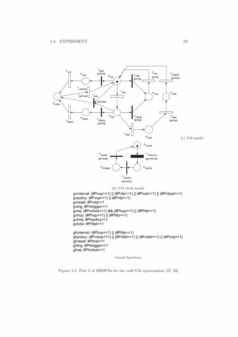
4.4. EXPERIMENT 63
Pvup
Pvfp
Pvfail
Pvrej Pvdet
Tvfail
Tvrej Tvrepair
Tvdet
Tvfp
Tvrejt
Tvfprejt
[gvtrig]
[gvtrig]
Pvsd
Pvfpsd
Tvsd
Tvfpsd
Pvstop
Tvfppre
Tvpre
[gvhrej]
[gvhrej]
Tvrestart
[gvhup]
[gvhdw]
Tvdw
[gvhup]
[gvhup]
[gvrej]
(c) VM model
Pvclock
PvpolicyPvtrigger
[gvpolicy]
Tvpolicy
[gvreset]
Tvreset[gvinterval]
Tvinterval
(d) VM clock model
gvinterval: (#Pvup==1) || (#Pvfp==1) || (#Pvsd==1) || (#Pvfpsd==1)gvpolicy: (#Pvup==1) || (#Pvfp==1)gvreset: #Pvrej==1gvtrig: #Pvtrigger==1gvrej: (#Pvclock==1) && (#Phup==1) || (#Phfp==1)gvhup: (#Phup==1) || (#Phfp==1)gvhrej: #Phpolicy==1gvhdw: #Phfail==1
ghinterval: (#Phup==1) || (#Phfp==1)ghpolicy: (#Pvstop==1) || (#Pvfail==1) || (#Pvdet==1) || (#Pvrej==1)ghreset: #Phrej==1ghtrig: #Phtrigger==1ghrej: #Phclock==1
Guard functions
Figure 4.2: Part 2 of MRSPNs for the cold-VM rejuvenation [37, 38].
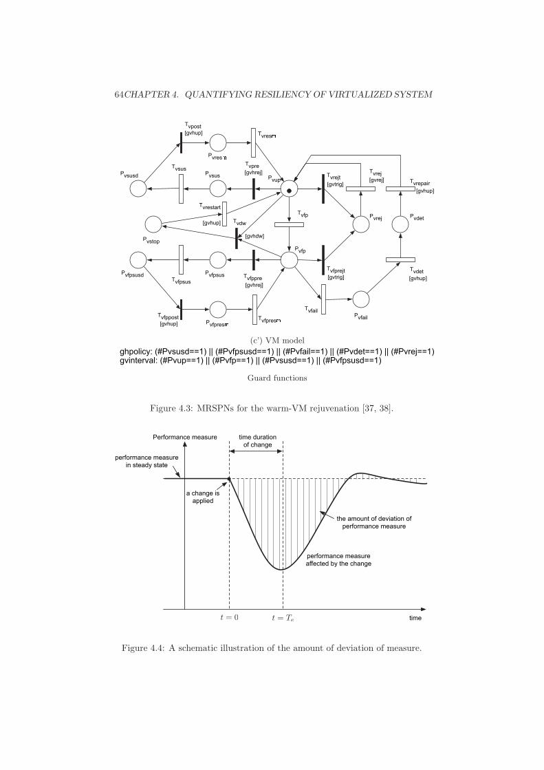
64CHAPTER 4. QUANTIFYING RESILIENCYOFVIRTUALIZED SYSTEM
Pvup
Pvfp
Pvfail
Pvrej Pvdet
Tvfail
TvrejTvrepair
Tvdet
Tvfp
Tvrejt
Tvfprejt
[gvtrig]
[gvtrig]
Pvsus
Pvfpsus
Tvsus
Tvfpsus
Pvstop
Tvfppre
Tvpre
[gvhrej]
[gvhrej]
Tvrestart
[gvhup]
[gvhdw]
Tvdw
Pvfpres"
Pvfpsusd
Pvsusd
Pvres"
Tvres"
Tvfpres"
Tvpost[gvhup]
Tvfppost[gvhup]
[gvhup]
[gvhup]
[gvrej]
(c’) VM model
Guard functions
Figure 4.3: MRSPNs for the warm-VM rejuvenation [37, 38].
Performance measure
performance measure in steady state
time duration of change
performance measure affected by the change
timet = 0 t = Te
the amount of deviation of performance measure
a change is applied
Figure 4.4: A schematic illustration of the amount of deviation of measure.

4.4. EXPERIMENT 65
0.75
0.8
0.85
0.9
0.95
1
0 20 40 60 80 100 120 140 160 180
avai
labi
lity
time (minutes)
cold (0.5)cold (1)cold (2)cold (7)
warm (0.5)warm (1)warm (2)warm (7)
Figure 4.5: The behavior of availabilities after the change (Te = 5 minutes)
0.75
0.8
0.85
0.9
0.95
1
0 20 40 60 80 100 120 140 160 180
avai
labi
lity
time (minutes)
cold (0.5)cold (1)cold (2)cold (7)
warm (0.5)warm (1)warm (2)warm (7)
Figure 4.6: The behavior of availabilities after the change (Te = 30 minutes)
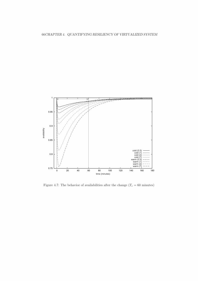
66CHAPTER 4. QUANTIFYING RESILIENCYOFVIRTUALIZED SYSTEM
0.75
0.8
0.85
0.9
0.95
1
0 20 40 60 80 100 120 140 160 180
avai
labi
lity
time (minutes)
cold (0.5)cold (1)cold (2)cold (7)
warm (0.5)warm (1)warm (2)warm (7)
Figure 4.7: The behavior of availabilities after the change (Te = 60 minutes)

Chapter 5
Conclusions
5.1 Summary and Remarks
In Chapter 2, we have dealt with the performance analysis of snapshot isola-
tion in the database system by using probabilistic models. We have developed
the models for CSI and PCSI and have derived the optimal time interval for
updating snapshot in PCSI with restart scheme under the failure-prone com-
munication environment. In the numerical examples, we have examined the
effectiveness of the optimization of update timing. As a result, although the
PCSI is effective to reduce the response time, the system throughput of PCSI
degrades, compared to CSI. The presence of communication failure discussed
in this paper is necessary and fundamental in the application of PCSI in dis-
tributed database system which has large network latency. With considering
the network environment, the usage of request restart scheme is supposed be
implemented in the database systems with small communication delay. In this
paper, we have revealed that the effect of communication failure on the perfor-
mance of distributed database system analytically. Furthermore, Monte Carlo
simulations have been conducted for investigating the effectiveness of our pro-
posal. The results of simulations indicated the effectiveness of our proposal. As
a conclusion of the comparison of CSI and PCSI, it can be implied that the CSI
is better at keeping the data integrity, and PCSI is better at improving the com-
munication effectiveness in distributed environment, especially when network is
crowed.
In Chapter 3, we have proposed an update management model for open
67
68 CHAPTER 5. CONCLUSIONS
source software from the customer’s point of view based on a non-homogeneous
Poisson process. We have also simply modeled user’s behavior on maintenance
activity based on non-homogeneous bug-discovery/correction processes by ap-
plying an unified software reliability model. As an extension of previous study,
[47] we have proposed a novel maintenance model in terms of the update cost
and recovery cost for users. By surmising users’ behavior, two maintenance
policies (periodic and aperiodic) have been discussed theoretically. For aperi-
odic policy, we derive the optimized maintenance schedule by DP algorithm. In
the numerical examples, we have examined the characteristics of two policies by
assuming two kinds of bug-correction processes, exponential and logistic. The
existences of optimized number of update times have been proven under both
policies. Moreover, based on the real bug data for Hadoop MapReduce, we
have shown that the optimized aperiodic maintenance policy is more effective
than the periodic one. However, we have just considered the patches for fixing
common bugs, i.e., fatal bugs or security holes are not taken into account. The
counteraction for emergent accidents must be the next topic of our research. On
the other hand, the best policy with consideration for both users and vendors
could be discussed in future.
In Chapter 4, we have evaluated the resiliency of the virtualized system with
software rejuvenation. In particular, we have defined one of the quantitative cri-
teria for evaluating the resiliency as the amount of deviation of measure, and
have presented how to compute it in CTMC models. In the experiment, we fo-
cused on the amount of deviation of system availability for the virtualized system
with software rejuvenation under two different rejuvenation policies. Since the
original model was described by MRSPNs, the model has been approximated by
a CTMC model through the PH expansion. Based on the scenario; the failure
rate of virtual machine increases, we have evaluated the resiliency of system. As
a result, we find that the time duration of change is insensitive to the system
availability, the system with cold-VM rejuvenation is more robust for the change
and the system with rejuvenation has the high ability of self-recovery. Besides,
we must notice that, the resiliency in this chapter is related as the deviation of
availability. If we change the performance index, the analysis of resiliency might
show us different results.
5.2. FUTURE WORKS 69
5.2 Future Works
Concerning PCSI, the parameters should be estimated from empirical data col-
lected in working database servers, and different servers have different values of
parameters. Thus we will discuss autonomic algorithms for deciding the optimal
time interval from empirical data based on the presented models in future.
For Chapter 4, we will investigate the resiliency of system under the migrate-
VM rejuvenation, and further analyze the system resiliency of a variety of system
such as checkpoint system and backup system in the future. Additionally, we
try to combine the resiliency analysis and fault-tree models and consider the
resiliency to disasters in the life-line system.

70 CHAPTER 5. CONCLUSIONS
Appendix A
EM-based PH fitting
This paper uses the PH fitting based on maximum likelihood (ML) estimation.
Briefly speaking, ML estimation is to determine the parameters minimizing
the Kullback-Leibler (KL) divergence. Given an arbitrary probability density
function f(t), the KL divergence KL(f, g) between f(t) and any probability
density function g(t) is defined by
KL(f, g) =
∫ ∞
0
f(t) logf(t)
g(t)dt
=
∫ ∞
0
f(t) log f(t)dt−
∫ ∞
0
f(t) log g(t)dt. (A.1)
The problem is to find g(t) maximizing∫∞
0f(t) log g(t)dt. Applying a suitable
numerical integration technique, we have
∫ ∞
0
f(t) log g(t)dt ≈
K∑
i=1
wi log g(ti), (A.2)
where wi, including f(ti), is a weight. The discretized points and their associ-
ated weights are computed by any numerical quadrature. Eq. (A.2) implies that
the parameter of g(t) are determined by the ordinary ML estimation with the
weighted samples (t1, w1), . . . , (tK , wK). In this paper, the weighted samples are
obtained from the numerical integration with the double exponential formula
[63].
On the other hand, this paper applies the EM (expectation-maximization)
algorithm to derive the ML estimations for PH distribution from weighted sam-
ples [46]. Fig. A.1 summaries one EM-step of the EM algorithm for PH distri-
butions with weighted samples (t1, w1), . . . , (tK , wK). In Fig. A.1, the symbols
[·]i and [·]i,j are the i-th entry of vector and (i, j)-entry of matrix, respectively.
71
72 APPENDIX A. EM-BASED PH FITTING
Also, ∆tk = tk − tk−1 is a time interval, q > maxi |[T ]i,i| is the maximum event
rate, the matrix P equals I +T/q with the identity matrix I, and Rk is a right
truncation point with tolerance error ε;
Rk∑
u=0
e−q∆tk(q∆tk)
u
u!≥ 1− ε. (A.3)
In Fig. A.1, the time complexity of the EM-step is O(ηK) where η is the number
of non-zero elements in T . This PH fitting algorithm in the paper can be utilized
by mapfit [50] as a package of statistical analysis tool R.

73
EM-step for PH fitting
1: Global step:
1.1 Forward: Compute ξk and αk for k = 1, . . . ,K;
αk ← αk−1 exp(T∆tk), α0 ← α,
ξk ← exp(T∆tk)ξk−1, ξ0 ← ξ.
1.2 Backward: Compute αk for k = K − 1, . . . , 1;
αk ← αk+1 exp(T∆tk+1) +wkα
αξk
,
αK ←wKα
αξK
.
2: Local step: For each time interval ∆tk, k = 1, . . . ,K;
2.1 Forward: Compute bu for u = 1, . . . , Rk;
bu ← Pbu−1, b0 ← ξk−1.
2.2 Backward: Compute cu for u = Rk − 1, . . . , 0;
cu ← cu+1P + e−q∆tk
(q∆tk)u+1
(u + 1)!αk,
cRk← e
−q∆tk(q∆tk)
Rk+1
(Rk + 1)!αk.
2.3 Aggregation: Compute Hk ←1q
∑Rku=0 bucu.
3: Aggregation: Compute H ←∑K
k=1 Hk.
4: Update:
[α]i ←
K∑
k=1
wk[α]i[ξk]i
αξk
/
K∑
k=1
wk,
[ξ]i ←K∑
k=1
wk[αu]i[ξ]i
αkξ
/
[H]i,i,
[T ]i,j ←[T ]i,j [H]j,i
[H]i,i, i 6= j.
Figure A.1: EM-based PH fitting with weighted samples [46].

74 APPENDIX A. EM-BASED PH FITTING

Bibliography
[1] A. A. Abdel-Ghaly, P. Y. Chan and B. Littlewood, Evaluation of competing
software reliability predictions, IEEE Trans. on Software Engineering, SE-
12(9), pp. 950–967, 1986.
[2] O. H. Alhazmi and Y. K. Malaiya, Modeling the vulnerability discovery
process, Proc. 16th International Symposium on Software Reliability Engi-
neering (ISSRE’05), IEEE CS Press, pp. 129–138, 2005.
[3] O. H. Alhazmi, Measuring and enhancing prediction capabilities of vul-
nerability discovery models for Apache and IIS HTTP servers, Proc. 17th
International Symposium on Software Reliability Engineering (ISSRE’06),
IEEE CS Press, pp. 343–352, 2006.
[4] O. H. Alhazmi and Y. K. Malaiya, Application of vulnerability discovery
models to major operating systems, IEEE Trans. on Reliability, vol. 57,
no. 1, pp. 14–22, 2008.
[5] A. Arora, R. Telang and H. Xu, Optimal policy for software vulnerability
disclosure, Third Annual Workshop on Economics of Information Security
(WEIS04), 2004.
[6] S. Asmussen and G. Koole, Marked point processes as limits of Markovian
arrival streams, Journal of Applied Probability, vol. 30, pp. 365–372, 1993.
[7] S. Beattie, S. Arnold, C. Cowan, P. Wagle and C. Wright, Timing the
application of security patches for optimal uptime, Proc. 16th USENIX
Systems Administration Conference (LISA02), pp. 233–242, 2002.
[8] R. Bellman, Dynamic Programming, Princeton University Press, 1957.
75

76 BIBLIOGRAPHY
[9] H. Berenson, P. Bernstein, J. Gray, J. Melton, E. O’Neil and P. O’Neil, A
critique of ANSI SQL isolation levels, Proc. of the SIGMOD International
Conference on Management of Data, pp. 1–10, ACM Press, 1995.
[10] J. M. Bernabe-Gisbert and V. Zuikeviciute, A probabilistic analysis of snap-
shot isolation with partial replication, Proc. of the 2008 Sympoisum on
Reliable Distributed Systems (SRDS-2008), pp. 249–258, IEEE CS Press,
2008.
[11] G. Bolch, S. Greiner, H. Meer and K. S. Trivedi, Queueing Networks and
Markov Chains: Modeling and Performance Evaluation with Computer Sci-
ence Applications, Wiley-Interscience, New York, 1998.
[12] B. Brykczynski and R. A. Small, Reducing Internet-based intru-
sions:Effective security patch management, IEEE Software, vol. 20, no.
1, pp. 50–57, 2003.
[13] H. Cavusoglu, Economics of security patch management, The Fifth Work-
shop on the Economics of Information Security (WEIS06), 2006.
[14] H. Cavusoglu and J. Zhang, Security patch management: Share the burden
or share the damage? Management Science, vol. 54, no. 4, pp. 657–670,
2008.
[15] A. Chervenak, I. Foster, C. Kesselman, C. Salisbury and S. Tuecke, The
data grid: Towards an architecture for the distributed management and
analysis of large scientific datasets. Journal of Network and Computer Ap-
plications, vol. 23, pp. 187–200, 2000.
[16] H. Choi, V. G. Kulkarni and K. S. Trivedi, Markov regenerative stochastic
Petri nets, Performance Evaluation, vol. 20, pp. 337–357, 1994.
[17] S. Dharmaraja, K. S. Trivedi, and D. Logothetis, Performance modeling
of wireless networks with generally distributed handoff interarrival times,
Computer Communications, vol. 26, no. 15, pp. 1747–1755, 2003.
[18] S. Elnikety, F. Pedone and W. Zwaenepoel, Database replication using
generalized snapshot isolation, Proc. of the 2005 Symposium on Reliable
Distributed Systems (SRDS-2005), pp. 73–84, IEEE CS Press, 2005.

BIBLIOGRAPHY 77
[19] D. P. Gaver, Observing stochastic processes and approximate transform
inversion, Operations Research, vol. 14, no. 3, pp. 444–459, 1966.
[20] R. German and C. Lindemann, Analysis of stochastic Petri nets by the
method of supplementary variables, Performance Evaluation, vol. 20, pp.
317–335, 1994.
[21] R. Ghosh, F. Longo, V. K. Naik, and K. S. Trivedi, Quantifying resiliency of
IaaS cloud, Proc. of 29th IEEE Symposium on Reliable Distributed Systems
(SRDS’10), pp. 343–347, IEEE CPS, 2010.
[22] A. L. Goel and K. Okumoto, Time-dependent error-detection rate model
for software reliability and other performance measures, IEEE Trans. on
Reliability, vol. R-28, pp. 206–211, 1979.
[23] A. L. Goel, Software reliability models: assumptions, limitations, and ap-
plicability, IEEE Trans. on Reliability, SE-11(12), pp. 1411–1423, 1985.
[24] S. S. Gokhale, M. R. Lyu and K. S. Trivedi, Software reliability analysis
incorporating fault detection and debugging activities, Proc. 9th Int’l Symp.
on Software Reliab. Eng., pp 202–211. IEEE CS Press, 1998.
[25] S. S. Gokhale, M. R. Lyu and K. S. Trivedi, Analysis of software fault
removal policies using a non-homogeneous continuous time Markov chain,
Software Quality Journal, 12(3), pp. 211–230, 2004.
[26] B. S. Gottfried, A stopping criterion for the golden-ratio search, Operations
Research, vol. 23, no. 3, pp. 553–555, 1975.
[27] R. Graham, S. E. Choi, D. Daniel, N. Desai, R. Minnich, C. Rasmussen, L.
Risinger and M. Sukalski, A network-failure-tolerant message-passing sys-
tem for terascale clusters. International Journal of Parallel Programming,
vol. 31, no. 4, pp. 285–303, 2003.
[28] J. Gray, A. Reuter, Transaction Processing: Concepts and Techniques, 1st
edn, Morgan Kaufmann Publishers Inc., San Francisco, CA, USA, 1992.
[29] M. Grottke and K. S. Trivedi, Fighting bugs: Remove, retry, replicate, and
rejuvenate, IEEE Computer, vol. 40, no. 2, pp. 107–109, 2007.
78 BIBLIOGRAPHY
[30] I. Hsieh, F. M. Chang and S. J. Kao, A slot-based bs scheduling with
maximum latency guarantee and capacity first in 802.16 e networks, In-
ternational Journal of Communication Systems, vol. 25, no. 2, pp. 55–66,
2012.
[31] Y. Huang, C. Kintala, N. Kolettis, and N. D. Fulton, Software rejuve-
nation:analysis, module and applications, Proc. 25th Int’l Sympo. Fault
Tolerant Computing, pp. 381–390, 1995.
[32] K. Kourai and S. Chiba, Fast software rejuvenation of virtual machine
monitor, IEEE Trans. on Dependable and Secure Computing, vol. 8, pp.
839–851, 2010.
[33] J. C. Laprie, From dependability to resilience, Proc. of 38th Annual
IEEE/IFIP International Conference on Dependable Systems and Networks
(DSN 2008), 2008.
[34] D. Logothetis and K. S. Trivedi, Transient analysis of the leaky bucket rate
control scheme under Poisson and ON-OFF sources, Proc. of?INFOCOM,
pp. 490–497, 1994.
[35] C. Luo, H. Okamura and T. Dohi, Model-based performance optimization
of generalized snapshot isolation in database system, Ubiquitous Intelli-
gence Computing and 9th International Conference on Autonomic Trusted
Computing (UIC/ATC 2012), pp. 494 –500, 2012.
[36] M. R. Lyu, Handbook of Software Reliability Engineering, New York:
McGraw-Hill, 1996.
[37] F. Machida, D. S. Kim, and K. S. Trivedi, Modeling and analysis of soft-
ware rejuvenation in a server virtualized system, Proc. of 2nd Workshop on
Software Aging and Rejuvenation (WoSAR2010), IEEE CS Press, 2010.
[38] F. Machida, D. S. Kim, and K. S. Trivedi, Modeling and analysis of soft-
ware rejuvenation in a server virtualized system with live VM migration,
Performance Evaluation, vol. 70, no. 3, pp. 212–230, 2013.

BIBLIOGRAPHY 79
[39] M. Marseguerra and E. Zio, Optimizing maintenance and repair policies via
a combination of genetic algorithms and Monte Carlo simulation, Reliability
Engineering and System Safety, vol. 68, no. 1, pp. 69–83, 2000.
[40] A. van Moorsel and K. Wolter, Analysis and algorithms for restart, Proc.
of Quantitative Evaluation of Systems, 2004. (QEST 2004), pp. 195–204,
2004.
[41] A. van Moorsel and K. Wolter, Analysis of restart mechanisms in software
systems, IEEE Trans. on Software Engineering, vol. 32, no. 8, pp. 547–558,
2006.
[42] J. D. Musa, A. Iannino and K. Okumoto, Software Reliability Measurement,
Prediction, Application, McGraw-Hill, New York, 1987.
[43] J. D. Musa, Software Reliability Engineering, McGraw-Hill, New York,
1999.
[44] M. Ohba, Inflection S-shaped software reliability growth model, Stochastic
Models in Reliability Theory, Springer-Verlag, Berlin, pp. 144–165, 1984.
[45] H. Okamura, T. Dohi and S. Osaki, EM algorithms for logistic software re-
liability models, Proc. 22nd IASTED International Conference on Software
Engineering, ACTA Press, pp. 263–268, 2004.
[46] H. Okamura, T. Dohi, and K. S. Trivedi, A refined EM algorithm for PH
distributions, Performance Evaluation, vol. 68, pp. 938–954, 2011.
[47] H. Okamura, M. Tokuzane and T. Dohi, Optimal Security Patch Release
Timing under Non-homogeneous Vulnerability-Discovery Processes, 20th
International Symposium on Software Reliability Engineering, (ISSRE’09),
pp. 120–128. 2009.
[48] H. Okamura and T. Dohi, Experience Report: SRATS: Software Reliability
Assessment Tool on Spreadsheet, Proc. of 24th IEEE International Sym-
posium on Software Reliability Engineering (ISSRE’13), IEEE Computer
Society Press, Pasadena, 2013.
80 BIBLIOGRAPHY
[49] H. Okamura, K. Yamamoto, and T. Dohi, Transient analysis of software re-
juvenation policies in virtualized system: Phase-type expansion approach,
Quality Technology and Quantitative Management, vol. 11, no. 3, pp 335–
351, 2014.
[50] H. Okamura and T. Dohi, mapfit: An R-based tool for PH/MAP param-
eter estimation, Proc. of 12th International Conference on Quantitative
Evaluation of Systems (QEST2015), 2015 (to appear).
[51] T. Ozsu and P. Valduriez, Principles of Distributed Database Systems,
Computer science, Springer, 2011.
[52] V. Padhye and A. Tripathi, Scalable transaction management with snap-
shot isolation on cloud data management systems, IEEE 5th International
Conference on Cloud Computing (CLOUD 2012), pp. 542–549, 2012.
[53] H. Pham, Handbook of Reliability Engineering, Springer, London, 2003.
[54] M. Puterman, Markov Decision Processes, John Wiley & Sons, 1994.
[55] S. Ramani, S. S. Gokhale and K. S. Trivedi, SREPT: software reliability
estimation and prediction tool, Performance Evaluation, vol. 39, issues 1?-
4, pp 37–60, 2000.
[56] D. Ramesh, A. Jain and C. Kumar, Implementation of atomicity and snap-
shot isolation for multi-row transactions on column oriented distributed
databases using rdbms, International Conference on Communications, De-
vices and Intelligent Systems (CODIS 2012), pp. 298–301, 2012.
[57] A. Reibman and K. S. Trivedi, Transient analysis of cumulative measures
of Markov model behavior, Stochastic Models, vol. 5, no. 4, pp. 683–710,
1989.
[58] S. M. Ross, Applied Probability Models with Optimization Applications,
Holden-Day, San Francisco, 1970.
[59] N. F. Schneidewind, Fault correction profiles, Proc. 14th Int’l Symp. on
Software Reliab. Eng., pp 257–267. IEEE CS Press, 2003.

BIBLIOGRAPHY 81
[60] N. F. Schneidewind, Assessing reliability risk using fault correction profiles,
Proc. 8th Int’l Symp. on High Assurance Systems Eng., pp 139–148. IEEE
CS Press, 2004.
[61] K. Shibata, K. Rinsaka, T. Dohi and H. Okamura, Quantifying soft-
ware maintainability based on a fault-detection/correction model, Proc.
of 13th Pacific Rim International Symposium on Dependable Computing
(PRDC’07), pp. 35–42, IEEE CPS, 2007.
[62] L. Simoncini, Resilient computing: An engineering discipline, Proc. of 23rd
IEEE International Symposium on Parallel and Distributed Processing, pp.
1, 2009.
[63] H. Takahasi and M. Mori, Double exponential formulas for numerical inte-
gration, Publ. RIMS, Kyoto Univ., vol. 9, pp. 721–741, 1974.
[64] M. Telek and A. Horvath, Transient analysis of Age-MRSPNs by the
method of supplementary variables, Performance Evaluation, vol. 45, pp.
205–221, 2001.
[65] P. P. Valko and J. Abate, Comparison of sequence accelerators for the gaver
method of numerical laplace transform inversion. Computers & Mathemat-
ics with Applications, vol. 48, no. 3, pp. 629–636, 2004.
[66] S. W. Woo, O. H. Alhazmi and Y. K. Malaiya, Assessing vulnerabilities in
Apache and IIS HTTP servers, Proc. 2nd IEEE International Symposium
on Dependable, Autonomic and Secure Computing (DASC’06), IEEE CS
Press, pp. 103–110, 2006.
[67] T. Xia, X. Jin, L. Xi and J. Ni, Production-driven opportunistic main-
tenance for batch production based on MAM?APB scheduling, European
Journal of Operational Research, vol. 240, no. 3, pp. 781–790, 2015.
[68] T. Xia, L. Xi, X. Zhou and J. Lee, Dynamic maintenance decision-making
for series?parallel manufacturing system based on MAM?MTW methodol-
ogy, European Journal of Operational Research, vol. 221, no. 1, pp. 231–240,
2012.

82 BIBLIOGRAPHY
[69] T. Xia, L. Xi, X. Zhou and S. Du, Modeling and optimizing maintenance
schedule for energy systems subject to degradation, Computers and Indus-
trial Engineering, vol. 63, no. 3, pp. 607–614, 2012.
[70] S. Yamada, M. Ohba and S. Osaki, S-shaped reliability growth modeling
for software error detection. IEEE Trans. on Reliability, vol. 32, no. 5, pp.
475–478, 1983.

Publication List of theAuthor
[1] C. Luo, H. Okamura, T. Dohi, Performance evaluation of snapshot isolation
in distributed database system under failure-prone environment, Journal of
Supercomputing, vol. 70, no. 3, pp. 1156–1179, Dec 2014.
[2] H. Okamura, J. Guan, C. Luo, T. Dohi, Quantifying Resiliency of Virtu-
alized System with Software Rejuvenation, IEICE Transactions on Funda-
mentals, vol.E98-A, no. 10, pp. 2051–2059, Oct 2015.
[3] C. Luo, H. Okamura, T. Dohi, Optimal Planning for Open Source Software
Updates, Journal of Risk and Reliability, vol. 230, no. 1, pp. 44–53, Feb
2016.
[4] C. Luo, H. Okamura, T. Dohi, Model-Based Performance Optimization of
Generalized Snapshot Isolation in Database System, Proc. of the 9th Inter-
national Conference on Ubiquitous Intelligence & Computing and the 9th
International Conference on Autonomic & Trusted Computing (UIC/ATC
2012), pp. 494–500, IEEE CS Press, Fukuoka, Japan, Sept 2012.
[5] C. Luo, H. Okamura, T. Dohi, Analysis of fairness in distributed database
system with snapshot isolation, The 18th IEEE Pacific Rim International
Symposium on Dependable Computing (PRDC 2012) (Fast Abstract), Ni-
igata, Japan, Nov 2012.
[6] C. Luo, H. Okamura, T. Dohi, Modeling and analysis of multi-version con-
current control, The 37th Annual International Computer Software and
Applications Conference (COMPSAC 2013), pp 53–58, Kyoto, Japan, Jul
2013.
83
84 PUBLICATION LIST OF THE AUTHOR
[7] C. Luo, H. Okamura, T. Dohi, Characteristic analysis of quantitative defi-
nition of resiliency measure, IEEE 24th International Symposium on Soft-
ware Reliability Engineering (ISSRE-2013) (Fast Abstract), pp 11–12, Los
Angeles, USA, Nov 2013.
[8] H. Okamura, C. Luo, T. Dohi, Estimating response time distribution of
server application in software aging phenomenon, IEEE 5th International
Workshop on Software Aging and Rejuvenation (WoSAR-2013), in con-
junction with The 24th IEEE International Symposium on Software Re-
liability Engineering (ISSRE-2013), pp 281–284, Los Angeles, USA, Nov
2013.
[9] H. Okamura, J. Guan, C. Luo, T. Dohi, Quantifying resiliency of virtual-
ized system with software rejuvenation, Proc. of The 2014 International
Conference on Quality, Reliability, Risk, Maintenance, and Safety Engi-
neering (QR2MSE 2014), 6 pages, 2014.
[10] C. Luo, H. Okamura, T. Dohi, Optimized patch applying schedule within
multiplex software architecture, The 6th Asia-Pacific International Sympo-
sium on Advanced Reliability and Maintenance Modeling (APARM 2014),
pp. 311–318, Sapporo, Japan, Aug 2014.