Embed Size (px)
Citation preview
Linkoping Studies in Science and TechnologyThesis No. 1061
A Survey and Comparison ofTime-Delay Estimation Methods
in Linear Systems
Svante Bjorklund
REGLERTEKNIK
AUTOMATIC CONTROL
LINKÖPING
Division of Automatic ControlDepartment of Electrical Engineering
Linkopings universitet, SE–581 83 Linkoping, SwedenWWW: http://www.control.isy.liu.se
Email: [email protected]
Linkoping 2003
A Survey and Comparison of Time-Delay Estimation Methods inLinear Systems
c© 2003 Svante Bjorklund
Department of Electrical Engineering,Linkopings universitet,SE–581 83 Linkoping,
Sweden.
ISBN 91-7373-870-0ISSN 0280-7971
LiU-TEK-LIC-2003:LIU-TEK-LIC-2003:60
Printed by UniTryck, Linkoping, Sweden 2003

To Ulrica

Abstract
In this thesis the problem of time-delay estimation (TDE) in linear dynamic systemsis treated. The TDE is studied for signal-to-noise ratios, input signals, and systemsthat are common in process industry. This also implies that both open-loop andclosed-loop cases are of interest. The true time-delay is estimated, which maybe different from the time-delay giving the best model approximation of the truesystem. Time-delays which are not a multiple of the sampling interval are also ofinterest to estimate.
In this thesis, a review and a classification according to underlying principlesof TDE methods in the literature are made. The main classes are: 1) Time-DelayApproximation Methods: The time-delay is estimated from a relation (a model)between the input and output signals expressed in a certain basis. The time-delay is not an explicit parameter in the model. 2) Explicit Time-Delay ParameterMethods: The time-delay is an explicit parameter in the model. 3) Area andMoment Methods: The time-delay is estimated from certain integrals of the impulseand step responses. 4) Higher Order Statistics Methods.
Some new methods and variants of old ones are suggested and evaluated, someof which have good estimation performance and some poor performance. Prop-erties of TDE methods are analyzed, both theoretically and experimentally. Rec-ommendations are given on how to choose estimation method and input signal.Generally, prediction error methods where the time-delay parameter is explicit andis optimized simultaneously with the other model parameters give good estimationquality.
Most evaluations have been conducted with factorial experiments using MonteCarlo simulations in open and closed loop. Some statistical analysis methods havebeen utilized: The RMS error of the time-delay estimates gives an absolute measureof the performance. ANOVA (ANalysis Of VAriance) and confidence intervals giveconclusions with a certain level of confidence.
i

Acknowledgements
First of all, I would like to thank my supervisor Professor Lennart Ljung for givingmy the possibility to join and get some insight into his successful research group andfor his skillful guidance in my own research. I am also very grateful to Professor AlfIsaksson, Dr. Alexander Horch and Professor Alexander Medvedev for discussingtime-delay estimation and sharing Matlab code with me. Professor Eva Enqvist,who first introduced me into ANOVA and some other statistical techniques, hasbeen very helpful and always found time for discussions. Thank you. I wouldlike to thank Martin Enqvist, Markus Gerdin, Jonas Gillberg, Frida Gunnarsson,David Lindgren, Dr. Jacob Roll, Ragnar Wallin for reading parts of different ver-sions of the manuscript and giving valuable comments. Thanks to Gustaf Hendebyand others for help with LATEX and to Jens Larsson and others for help with ourcomputer systems. Ulla Salaneck deserves gratitude for always being helpful withadministrative matters. Thanks to all members of the Control and Communicationgroup for creating a nice working atmosphere. This work has been supported bythe Swedish Research Council, which is hereby gratefully acknowledged.
Svante BjorklundLinkoping, November 2003
iii

iv
Contents
1 Introduction 31.1 The Problem . . . . . . . . . . . . . . . . . . . . . . . . . . . . . . . 31.2 Purpose . . . . . . . . . . . . . . . . . . . . . . . . . . . . . . . . . . 41.3 Contributions . . . . . . . . . . . . . . . . . . . . . . . . . . . . . . . 41.4 Outline . . . . . . . . . . . . . . . . . . . . . . . . . . . . . . . . . . 5
I Time-delay estimation problems and methods 7
2 Time-delay Estimation Problems and Time-Delay Systems 92.1 Time-Delay Estimation Problems . . . . . . . . . . . . . . . . . . . 92.2 Time-Delay Systems . . . . . . . . . . . . . . . . . . . . . . . . . . . 11
3 Classes of Active Time-Delay Estimation Methods 13
4 Time-Delay Approximation Methods 154.1 Time Domain Approximation Methods (Thresholding Methods) . . 15
4.1.1 Principles . . . . . . . . . . . . . . . . . . . . . . . . . . . . . 154.1.2 Estimating the approximation model . . . . . . . . . . . . . 174.1.3 Estimating the start of the impulse response . . . . . . . . . 194.1.4 Separating the time-delay and the dynamics . . . . . . . . . 234.1.5 Relation between PEM, cross-correlation, matched filter and
maximum likelihood estimation . . . . . . . . . . . . . . . . 254.1.6 Some methods . . . . . . . . . . . . . . . . . . . . . . . . . . 27
v
vi
4.2 Frequency Domain Approximation Methods (Phase Methods) . . . 284.2.1 Time-delay in continuous-time . . . . . . . . . . . . . . . . . 284.2.2 Time-delay in discrete-time . . . . . . . . . . . . . . . . . . . 284.2.3 Estimating the approximation model . . . . . . . . . . . . . 304.2.4 Continuous-time estimation using Pade approximation . . . 304.2.5 Using the phase of the discrete-time allpass part (DAP meth-
ods) . . . . . . . . . . . . . . . . . . . . . . . . . . . . . . . . 314.2.6 Problems with the DAP method . . . . . . . . . . . . . . . . 324.2.7 A solution to the problem with the DAP method . . . . . . 35
4.3 Laguerre Domain Approximation Methods . . . . . . . . . . . . . . 374.3.1 The discrete-time Laguerre domain . . . . . . . . . . . . . . 374.3.2 System representation in the discrete-time Laguerre domain 394.3.3 Two discrete-time Laguerre domain time-delay estimation al-
gorithms . . . . . . . . . . . . . . . . . . . . . . . . . . . . . 404.3.4 Approximating the signals with the Laguerre transform . . . 40
5 Explicit Time-Delay Parameter Methods 435.1 Continuous-Time One-Step Explicit Methods . . . . . . . . . . . . . 43
5.1.1 The time-delay estimation methods . . . . . . . . . . . . . . 435.1.2 Local minima of a first order system . . . . . . . . . . . . . . 445.1.3 Widening the region of convergence by low-pass filtering . . 48
5.2 Discrete-Time One-Step Explicit Methods . . . . . . . . . . . . . . 505.2.1 Arxstruc . . . . . . . . . . . . . . . . . . . . . . . . . . . . . 505.2.2 Oestruc . . . . . . . . . . . . . . . . . . . . . . . . . . . . . . 515.2.3 Met1struc . . . . . . . . . . . . . . . . . . . . . . . . . . . . 51
5.3 Sampling Methods . . . . . . . . . . . . . . . . . . . . . . . . . . . . 555.3.1 Principles . . . . . . . . . . . . . . . . . . . . . . . . . . . . . 555.3.2 Recursive TIDEA . . . . . . . . . . . . . . . . . . . . . . . . 565.3.3 Exact time-delay from the sampling process . . . . . . . . . 57
6 Area, Moment and Higher-Order Statistics Methods 596.1 Area Methods . . . . . . . . . . . . . . . . . . . . . . . . . . . . . . 596.2 Moment Methods . . . . . . . . . . . . . . . . . . . . . . . . . . . . 606.3 An Area and Moment Method with Better Noise Properties . . . . 616.4 Higher-Order Statistics Methods . . . . . . . . . . . . . . . . . . . . 62
II Comparison and properties of time-delay estimationmethods 63
7 Simulation Setup and Analysis 657.1 Factorial Experiments . . . . . . . . . . . . . . . . . . . . . . . . . . 657.2 Implementation of Estimation Methods . . . . . . . . . . . . . . . . 667.3 Open Loop Simulation Setup . . . . . . . . . . . . . . . . . . . . . . 69
7.3.1 A standard benchmark . . . . . . . . . . . . . . . . . . . . . 72
vii
7.4 Closed Loop Simulation Setup . . . . . . . . . . . . . . . . . . . . . 737.5 Analysis Methods . . . . . . . . . . . . . . . . . . . . . . . . . . . . 75
7.5.1 Managing failing estimates . . . . . . . . . . . . . . . . . . . 767.5.2 Plots of RMS error, bias and standard deviation . . . . . . . 777.5.3 ANOVA and confidence intervals . . . . . . . . . . . . . . . . 77
8 Parameters and Properties of Estimation Methods 858.1 Time Domain Approximation Methods . . . . . . . . . . . . . . . . 85
8.1.1 Choosing parameters in thresholding methods . . . . . . . . 858.1.2 Properties of thresholding methods . . . . . . . . . . . . . . 86
8.2 Frequency Domain Approximation Methods . . . . . . . . . . . . . 888.2.1 DAP in open loop . . . . . . . . . . . . . . . . . . . . . . . . 888.2.2 More properties of DAP methods . . . . . . . . . . . . . . . 908.2.3 Discussion . . . . . . . . . . . . . . . . . . . . . . . . . . . . . 918.2.4 Conclusions . . . . . . . . . . . . . . . . . . . . . . . . . . . 92
8.3 Laguerre Domain Approximation Methods . . . . . . . . . . . . . . 938.3.1 The standard benchmark . . . . . . . . . . . . . . . . . . . . 938.3.2 Several Laguerre domain approximation methods with step
input . . . . . . . . . . . . . . . . . . . . . . . . . . . . . . . 938.3.3 The method fischer8 with step input signals . . . . . . . . . 948.3.4 Execution time . . . . . . . . . . . . . . . . . . . . . . . . . . 958.3.5 Discussion . . . . . . . . . . . . . . . . . . . . . . . . . . . . 968.3.6 Conclusions . . . . . . . . . . . . . . . . . . . . . . . . . . . 97
8.4 Continuous-Time One-Step Explicit Methods (Idproc Methods) . . 988.5 Discrete-Time One-Step Explicit Methods . . . . . . . . . . . . . . 99
8.5.1 Choice of parameters in arxstruc type methods . . . . . . . . 998.5.2 More properties of arxstruc type methods . . . . . . . . . . . 1018.5.3 Discussion . . . . . . . . . . . . . . . . . . . . . . . . . . . . 102
8.6 Area and Moment Methods . . . . . . . . . . . . . . . . . . . . . . . 104
9 Comparing Time-Delay Estimation Methods in Open and ClosedLoop 1079.1 Open Loop Simulations with Fixed Systems . . . . . . . . . . . . . 107
9.1.1 The standard benchmark . . . . . . . . . . . . . . . . . . . . 1079.1.2 Confidence intervals for step input . . . . . . . . . . . . . . . 109
9.2 Open Loop Simulations with Random Systems . . . . . . . . . . . . 1119.3 Comparing the time-delay estimation methods in closed loop . . . . 112
9.3.1 Closed loop simulation results . . . . . . . . . . . . . . . . . 1129.3.2 Discussion . . . . . . . . . . . . . . . . . . . . . . . . . . . . 113
9.4 Execution Time . . . . . . . . . . . . . . . . . . . . . . . . . . . . . 114
10 Discussion and Conclusions 11710.1 Additional Discussion about Open Loop . . . . . . . . . . . . . . . . 11710.2 Recommendations for Choice of Estimation Method . . . . . . . . . 11810.3 Conclusions about Parameters and Properties of Methods . . . . . . 119
viii Contents
10.4 Future Work . . . . . . . . . . . . . . . . . . . . . . . . . . . . . . . 122
Bibliography 123
A ANOVA and Confidence Interval Validation 131A.1 Validation of ANOVA and Confidence Intervals for Time Domain
Methods . . . . . . . . . . . . . . . . . . . . . . . . . . . . . . . . . 131A.1.1 Choosing parameters of direct thresholding of impulse re-
sponse . . . . . . . . . . . . . . . . . . . . . . . . . . . . . . 131A.1.2 Properties of direct thresholding of impulse response . . . . 131
A.2 Properties of DAP Methods . . . . . . . . . . . . . . . . . . . . . . 133A.3 Validation of ANOVA and Confidence Intervals for Laguerre Domain
Methods . . . . . . . . . . . . . . . . . . . . . . . . . . . . . . . . . 134A.3.1 Several Laguerre domain approximation methods with only
steps . . . . . . . . . . . . . . . . . . . . . . . . . . . . . . . 134A.3.2 The method fischer8 with step input signals at low SNR . . 136
A.4 Validation of ANOVA and Confidence Intervals for Idproc Methods 136A.5 Validation of ANOVA and Confidence Intervals for Arxstruc Type
Methods . . . . . . . . . . . . . . . . . . . . . . . . . . . . . . . . . 141A.6 Validation for Promising Methods with Only Steps and SNR =1 . . 141
List of Figures
4.1 The creation of the impulse response of a system with time-delay. . 164.2 Estimation of time-delay by the start of the impulse response. . . . . 174.3 Impulse response estimates of the system G1. . . . . . . . . . . . . . 194.4 Steps in time-delay estimation in the time domain. . . . . . . . . . 204.5 Direct thresholding of impulse response. . . . . . . . . . . . . . . . . 214.6 CUSUM thresholding of impulse response. . . . . . . . . . . . . . . . 224.7 Separating the dynamics from the pure time delay. . . . . . . . . . . 244.8 Poles & zeros of Laguerre model for successful and failing estimation. 344.9 Time-delay estimate for different zero locations. . . . . . . . . . . . . 364.10 Pole-zero plot with uncertainty and simulated poles & zeros. . . . . 374.11 Laguerre functions in discrete time. . . . . . . . . . . . . . . . . . . . 384.12 Original and Laguerre approximated input and output signals. . . . 42
5.1 Loss function for true time-delay 0.1Ts. . . . . . . . . . . . . . . . . 465.2 Loss function for true time-delay (2/3)Ts and 0.9Ts . . . . . . . . . . 475.3 Loss function for true time-delay 0.9999Ts. . . . . . . . . . . . . . . 485.4 Part of the second derivative of the loss function. . . . . . . . . . . . 49
7.1 Impulse response of systems G1-G2 and G5-G8. . . . . . . . . . . . . 717.2 The input signal RBS 10-30%. . . . . . . . . . . . . . . . . . . . . . . 727.3 The input signal RBS 0-100%. . . . . . . . . . . . . . . . . . . . . . . 727.4 The input signal Steps. . . . . . . . . . . . . . . . . . . . . . . . . . . 737.5 The control system in closed loop simulations. . . . . . . . . . . . . 747.6 Example of plot of RMS error. . . . . . . . . . . . . . . . . . . . . . 787.7 Example of plot for choosing a variance-stabilizing transform. . . . . 80
ix
x Contents
7.8 Example of confidence interval plot. . . . . . . . . . . . . . . . . . . 827.9 Example of residual analysis for ANOVA and confidence intervals. . 837.10 Example plots of residual standard deviation versus factor levels. . . 84
8.1 Confidence intervals for parameters in idimp4. . . . . . . . . . . . . . 868.2 Confidence intervals for comparing different thresholding methods. . 878.3 RMS error of DAP methods without zero guarding. . . . . . . . . . 898.4 RMS error of DAP methods with zero guarding. . . . . . . . . . . . 908.5 Confidence intervals for properties of DAP methods. . . . . . . . . . 918.6 RMS errors for Laguerre domain methods. . . . . . . . . . . . . . . 948.7 Confidence intervals for Laguerre domain methods with step input. 958.8 Confidence intervals for different systems for fischer8 with step input. 968.9 Confidence intervals in idproc methods for model structures & prewhiten-
ing. . . . . . . . . . . . . . . . . . . . . . . . . . . . . . . . . . . . . . 998.10 Confidence intervals in idproc methods for input signal and system. 1008.11 RMS error for arxstruc as a function of model orders. . . . . . . . . . 1018.12 RMS error for oestruc as a function of model orders. . . . . . . . . . 1028.13 RMS error for met1struc as a function of model orders. . . . . . . . . 1038.14 Confidence intervals for properties of arxstruc type methods. . . . . 103
9.1 RMS error for different methods in open loop with fixed systems. . . 1089.2 RMS error for different methods, SNR and input signal types in open
loop with fixed systems. . . . . . . . . . . . . . . . . . . . . . . . . . 1099.3 RMS error for different methods and systems in open loop with fixed
systems. . . . . . . . . . . . . . . . . . . . . . . . . . . . . . . . . . . 1109.4 Confidence intervals for promising methods with step input in open
loop. . . . . . . . . . . . . . . . . . . . . . . . . . . . . . . . . . . . 1119.5 RMS error for different methods on random systems in open loop. . 1129.6 RMS error for different methods in closed loop. . . . . . . . . . . . . 1139.7 RMS error for different methods and systems in closed loop. . . . . . 1149.8 RMS error for different methods and controllers in closed loop. . . . 1159.9 RMS error for different methods and noise models in closed loop. . . 116
10.1 Classes of active time-delay estimation methods. . . . . . . . . . . . 119
A.1 Transform for ANOVA for choosing parameters in the method idimp4.132A.2 Residual analysis for choosing parameters in the method idimp4. . . 132A.3 Residual standard deviation for choosing parameters in the method
idimp4. . . . . . . . . . . . . . . . . . . . . . . . . . . . . . . . . . . . 134A.4 Transform for ANOVA for studying properties of the method idimp4. 135A.5 Residual analysis for studying properties of the method idimp4. . . . 135A.6 Residual standard deviation for studying properties of the method
idimp4. . . . . . . . . . . . . . . . . . . . . . . . . . . . . . . . . . . . 136A.7 Transform for ANOVA for studying properties of DAP methods. . . 137A.8 Residual analysis for studying properties of DAP methods. . . . . . 137
Contents xi
A.9 Residual standard deviation for studying properties of DAP methods.138A.10 Transform for ANOVA for Laguerre domain approximation methods
with input signal Steps. . . . . . . . . . . . . . . . . . . . . . . . . . 138A.11 Residual analysis for several Laguerre domain approximation meth-
ods with input signal Steps. . . . . . . . . . . . . . . . . . . . . . . 139A.12 Residual standard deviation for several Laguerre domain approxi-
mation methods with input signal Steps. . . . . . . . . . . . . . . . 139A.13 Transform and residual standard deviation for fischer8 with input
Steps. . . . . . . . . . . . . . . . . . . . . . . . . . . . . . . . . . . . 140A.14 Residual analysis for fischer8 with input signal Steps. . . . . . . . . . 140A.15 Transform for ANOVA of all idproc methods. . . . . . . . . . . . . . 142A.16 Residual analysis for all idproc methods. . . . . . . . . . . . . . . . . 142A.17 Residual standard deviation for all idproc methods. . . . . . . . . . . 143A.18 Transform for ANOVA of properties of arxstruc type methods. . . . 144A.19 Residual analysis for properties of arxstruc type methods. . . . . . . 144A.20 Residual standard deviation for properties of arxstruc type methods. 145A.21 Transform for ANOVA for some promising methods with input signal
Steps in open loop. . . . . . . . . . . . . . . . . . . . . . . . . . . . . 145A.22 Residual analysis for some promising methods with input signal
Steps in open loop. . . . . . . . . . . . . . . . . . . . . . . . . . . . . 146A.23 Residual standard deviation for some promising methods with input
signal Steps in open loop. . . . . . . . . . . . . . . . . . . . . . . . . 146

xii Contents
List of Tables
4.1 Internal variables for the DAP method for a successful, a failing anda zero guarded estimation. . . . . . . . . . . . . . . . . . . . . . . . . 34
7.1 Parameters of implemented Laguerre domain approximation meth-ods. . . . . . . . . . . . . . . . . . . . . . . . . . . . . . . . . . . . . 68
7.2 Example of ANOVA table. . . . . . . . . . . . . . . . . . . . . . . . . 80
8.1 Execution time for fischer8 and arxstruc3. . . . . . . . . . . . . . . . 96
9.1 Execution time for many methods. . . . . . . . . . . . . . . . . . . . 116
10.1 Better system and input signal for different classes of methods. . . . 120
A.1 ANOVA table for choosing parameters in the method idimp4. . . . . 133A.2 ANOVA table for studying properties of the method idimp4. . . . . . 133A.3 ANOVA table for studying properties of DAP methods. . . . . . . . 134A.4 ANOVA table for Laguerre domain approximation methods with
input signal Steps. . . . . . . . . . . . . . . . . . . . . . . . . . . . . 136A.5 ANOVA table for fischer8 with input Steps. . . . . . . . . . . . . . . 138A.6 ANOVA table for all idproc methods. . . . . . . . . . . . . . . . . . 141A.7 ANOVA table for properties of Arxstruc type methods. . . . . . . . 143A.8 ANOVA table for some promising methods with input signal Steps
in open loop. . . . . . . . . . . . . . . . . . . . . . . . . . . . . . . . 143
xiii

xiv Contents
List of Algorithms
1 CUSUM detector. . . . . . . . . . . . . . . . . . . . . . . . . . . . . 212 Direct and CUSUM thresholding of impulse or step response with
relative threshold. . . . . . . . . . . . . . . . . . . . . . . . . . . . . 273 tausvd: An implementation of Laguerre domain approximation method. 414 taulp1: Another implementation of Laguerre domain approximation
method. . . . . . . . . . . . . . . . . . . . . . . . . . . . . . . . . . . 415 Matlab code for arxstructd . . . . . . . . . . . . . . . . . . . . . . . 516 Matlab code for oestructd. . . . . . . . . . . . . . . . . . . . . . . . 517 Proposed time-delay estimation method (prefiltered arxstruc). . . . 538 met1struc, the prefiltered arxstruc. . . . . . . . . . . . . . . . . . . . 549 Matlab code for met1struc. . . . . . . . . . . . . . . . . . . . . . . . 5410 Prewhitening the input signal. . . . . . . . . . . . . . . . . . . . . . 70
xv

xvi Contents
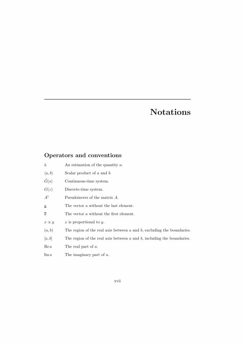
Notations
Operators and conventions
a An estimation of the quantity a.
〈a, b〉 Scalar product of a and b.
G(s) Continuous-time system.
G(z) Discrete-time system.
A† Pseudoinvers of the matrix A.
a The vector a without the last element.
a The vector a without the first element.
x ∝ y x is proportional to y.
(a, b) The region of the real axis between a and b, excluding the boundaries.
[a, b] The region of the real axis between a and b, including the boundaries.
Rea The real part of a.
Im a The imaginary part of a.
xvii
xviii Contents
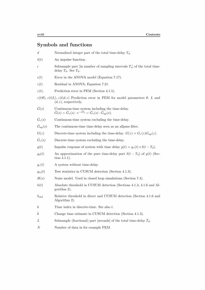
Symbols and functions
d Normalized integer part of the total time-delay Td.
δ(t) An impulse function.
ε Subsample part [in number of sampling intervals Ts] of the total time-delay Td. See Td.
ε(t) Error in the ANOVA model (Equation 7.17).
ε(t) Residual in ANOVA, Equation 7.21.
ε(t), Prediction error in PEM (Section 4.1.5).
ε(t|θ), ε(t|L), ε(t|d, ε) Prediction error in PEM for model parameters θ, L and(d, ε), respectively.
G(s) Continuous-time system including the time-delay.G(s) = Gr(s) · e−sTd = Gr(s) · Gap(s).
Gr(s) Continuous-time system excluding the time-delay.
Gap(s) The continuous-time time-delay seen as an allpass filter.
G(z) Discrete-time system including the time-delay. G(z) = Gr(z)Gap(z).
Gr(s) Discrete-time system excluding the time-delay.
g(t) Impulse response of system with time delay g(t) = gr(t) ∗ δ(t− Td).
gd(t) An approximation of the pure time-delay part δ(t − Td) of g(t) (Sec-tion 4.1.1).
gr(t) A system without time-delay.
gts(t) Test statistics in CUSUM detection (Section 4.1.3).
H(s) Noise model. Used in closed loop simulations (Section 7.4).
h(t) Absolute threshold in CUSUM detection (Sections 4.1.3, 4.1.6 and Al-gorithm 2).
hstd Relative threshold in direct and CUSUM detection (Section 4.1.6 andAlgorithm 2).
k Time index in discrete-time. See also t.
k Change time estimate in CUSUM detection (Section 4.1.3).
L Subsample (fractional) part [seconds] of the total time-delay Td.
N Number of data in for example PEM.
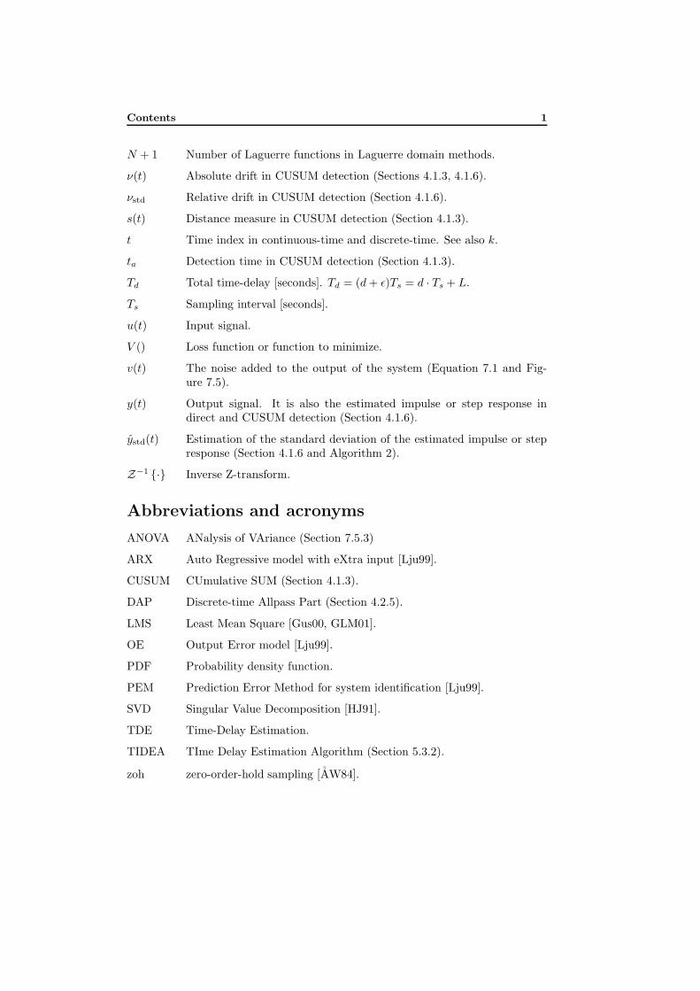
Contents 1
N + 1 Number of Laguerre functions in Laguerre domain methods.
ν(t) Absolute drift in CUSUM detection (Sections 4.1.3, 4.1.6).
νstd Relative drift in CUSUM detection (Section 4.1.6).
s(t) Distance measure in CUSUM detection (Section 4.1.3).
t Time index in continuous-time and discrete-time. See also k.
ta Detection time in CUSUM detection (Section 4.1.3).
Td Total time-delay [seconds]. Td = (d+ ε)Ts = d · Ts + L.
Ts Sampling interval [seconds].
u(t) Input signal.
V () Loss function or function to minimize.
v(t) The noise added to the output of the system (Equation 7.1 and Fig-ure 7.5).
y(t) Output signal. It is also the estimated impulse or step response indirect and CUSUM detection (Section 4.1.6).
ystd(t) Estimation of the standard deviation of the estimated impulse or stepresponse (Section 4.1.6 and Algorithm 2).
Z−1 {·} Inverse Z-transform.
Abbreviations and acronyms
ANOVA ANalysis of VAriance (Section 7.5.3)
ARX Auto Regressive model with eXtra input [Lju99].
CUSUM CUmulative SUM (Section 4.1.3).
DAP Discrete-time Allpass Part (Section 4.2.5).
LMS Least Mean Square [Gus00, GLM01].
OE Output Error model [Lju99].
PDF Probability density function.
PEM Prediction Error Method for system identification [Lju99].
SVD Singular Value Decomposition [HJ91].
TDE Time-Delay Estimation.
TIDEA TIme Delay Estimation Algorithm (Section 5.3.2).
zoh zero-order-hold sampling [AW84].
2 Contents
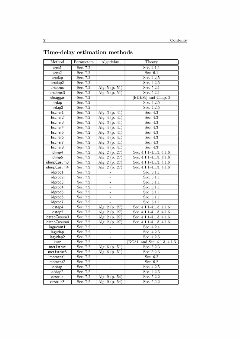
Time-delay estimation methods
Method Parameters Algorithm Theory
area1 Sec. 7.2 - Sec. 4.1.1area2 Sec. 7.2 - Sec. 6.1
arxdap Sec. 7.2 - Sec. 4.2.5arxdap2 Sec. 7.2 - Sec. 4.2.5arxstruc Sec. 7.2 Alg. 5 (p. 51) Sec. 5.2.1
arxstruc3 Sec. 7.2 Alg. 5 (p. 51) Sec. 5.2.1elnaggar Sec. 7.2 - [EDE89] and Chap. 3
firdap Sec. 7.2 - Sec. 4.2.5firdap2 Sec. 7.2 - Sec. 4.2.5fischer1 Sec. 7.2 Alg. 3 (p. 41) Sec. 4.3fischer2 Sec. 7.2 Alg. 4 (p. 41) Sec. 4.3fischer3 Sec. 7.2 Alg. 3 (p. 41) Sec. 4.3fischer4 Sec. 7.2 Alg. 4 (p. 41) Sec. 4.3fischer5 Sec. 7.2 Alg. 3 (p. 41) Sec. 4.3fischer6 Sec. 7.2 Alg. 4 (p. 41) Sec. 4.3fischer7 Sec. 7.2 Alg. 3 (p. 41) Sec. 4.3fischer8 Sec. 7.2 Alg. 4 (p. 41) Sec. 4.3idimp4 Sec. 7.2 Alg. 2 (p. 27) Sec. 4.1.1-4.1.3, 4.1.6idimp5 Sec. 7.2 Alg. 2 (p. 27) Sec. 4.1.1-4.1.3, 4.1.6
idimpCusum3 Sec. 7.2 Alg. 2 (p. 27) Sec. 4.1.1-4.1.3, 4.1.6idimpCusum4 Sec. 7.2 Alg. 2 (p. 27) Sec. 4.1.1-4.1.3, 4.1.6
idproc1 Sec. 7.2 - Sec. 5.1.1idproc2 Sec. 7.2 - Sec. 5.1.1idproc3 Sec. 7.2 - Sec. 5.1.1idproc4 Sec. 7.2 - Sec. 5.1.1idproc5 Sec. 7.2 - Sec. 5.1.1idproc6 Sec. 7.2 - Sec. 5.1.1idproc7 Sec. 7.2 - Sec. 5.1.1idstep4 Sec. 7.2 Alg. 2 (p. 27) Sec. 4.1.1-4.1.3, 4.1.6idstep5 Sec. 7.2 Alg. 2 (p. 27) Sec. 4.1.1-4.1.3, 4.1.6
idstepCusum3 Sec. 7.2 Alg. 2 (p. 27) Sec. 4.1.1-4.1.3, 4.1.6idstepCusum4 Sec. 7.2 Alg. 2 (p. 27) Sec. 4.1.1-4.1.3, 4.1.6
lagucont1 Sec. 7.2 - Sec. 4.2.4lagudap Sec. 7.2 - Sec. 4.2.5
lagudap2 Sec. 7.2 - Sec. 4.2.5kurz Sec. 7.2 - [KG81] and Sec. 4.1.3, 4.1.6
met1struc Sec. 7.2 Alg. 6 (p. 51) Sec. 5.2.3met1struc3 Sec. 7.2 Alg. 6 (p. 51) Sec. 5.2.3moment1 Sec. 7.2 - Sec. 6.2moment2 Sec. 7.2 - Sec. 6.2
oedap Sec. 7.2 - Sec. 4.2.5oedap2 Sec. 7.2 - Sec. 4.2.5oestruc Sec. 7.2 Alg. 9 (p. 54) Sec. 5.2.2
oestruc3 Sec. 7.2 Alg. 9 (p. 54) Sec. 5.2.2
1Introduction
This chapter defines the problem that is treated in this thesis, states the purposewith this work, lists the main contributions in and gives an outline of this thesis.
1.1 The Problem
In this thesis we will study the time-delay estimation (TDE) problem, where wewant to estimate Td in
y(t) = G(p)u(t) + n(t) = Gr(p)u(t− Td) + n(t), (1.1)
where the system Gr(p) is a SISO (single-input single-output) time-invariant lineartransfer function without time-delay. In signal processing applications, the systemis often restricted to be a constant [C+81, MG+98], but here Gr(p) will be atransfer function with dynamics, of the type which typical in process industry, seee.g. [IHD01b, Swa99]. This means that both the open-loop and closed-loop casesare of interest and that we will study TDE for SNRs (signal-to-noise ratio), inputsignals and systems, that are common in such applications.
We are only interested in the estimation of the time-delay. Some methods alsoestimate the other parameters needed for a complete model of G(p). We considerthese other parameters as nuisance. When estimating the time-delay, the objectivecan be either of the following two:
1. Estimate the best approximation time-delay , i.e. the time-delay estimate thatgives the “best” model approximation of the true system. What is “best”depends on the intended use of the model and can be measured in many
3
4 Chapter 1 Introduction
different ways. In automatic control, the time-delay estimate can be a meansto achieve a good model in the frequency band relevant to the control [Lju02,FMS91], e.g. around the cross-over frequency. It is possible to choose thefrequency band where to achieve a good model by designing the input signalspectrum and/or prefiltering the data [Lju99, Lju02]. In [Swa99] the apparenttime-delay (the delay resulting from identifying a first order model with time-delay from the data) is used for control performance monitoring of PID controlloops.
2. Estimate the true time-delay (Td in Equation (1.1)). This is the case in “puretime-delay” estimation, diagnosis, radar range estimation [KQ92, Sum95],direction of arrival estimation with array antennas [HR97, Wik02, FHJ02],measuring blood velocity [LT99], averaging of measured signals [GS94] etc.
Since we have not decided on a special use of the time-delay estimate, we will inthis thesis evaluate estimation methods according to the second objective.
We consider it as an advantage if a method can estimate time-delays that alsoconsist of fractions of the sampling interval. However, some methods can onlyestimate time-delays that are a multiple of the sampling interval. Sometimes suchmethods can be used to initialize other more “free” methods.
Time-delay estimation has been studied in the literature for a long time, espe-cially for pure time-delay systems [C+81, Car87, Car93] but also for systems with
dynamics [AH95, CHWW99, EDE89, FMS91, Hor00, Isa97, KG81, Lju02, NL91,Pup85, WZ01, Swa99, IHD01b, IHD00]. However, there is still no clear agreementon which method is “best” for systems with dynamics.
1.2 Purpose
The purpose of this thesis is to:
1. Review and classify existing time-delay estimation methods for dynamics sys-tems according to their underlying principles.
2. Try to find the “best” time-delay estimation method for dynamic systems fordifferent cases by comparing the quality of the estimates of methods usingsimulated data.
1.3 Contributions
The main contributions of this thesis are
1. Statement of a general time-delay estimation problem in linear systems en-compassing both automatic control and signal processing applications (Equa-tion 2.1).
1.4 Outline 5
2. Classification of existing time-delay estimation methods into classes with com-mon principles and pointing out connections between the classes (Chapters 3-6).
3. Serious comparison of several time-delay estimation methods using confidenceintervals and other methods on Monte Carlo simulated data to see whichmethod is the the best and which method to use in which case (Sections 8-9).
4. Properties of classes of methods from simulations.
5. Some theoretical properties of local minima for explicit time-delay parametermethods using first order model with time-delay (Section 5.1.2).
6. Improvements and modifications of old and development of new time-delayestimation methods:
(a) Zero guarding for making phase methods more robust (Section 4.2.7).
(b) The prefiltered Arxstruc method met1struc (Section 5.2.3).
(c) Exact time-delay from the sampling process (Section 5.3.3).
(d) CUSUM thresholding on impulse and step response estimates (Section4.1.6).
(e) Area and moment methods on estimated step and impulse responsesinstead of measured ones (Section 6.1-6.2).
(f) A cepstrum-like method for the separation of the time-delay from thedynamics of a linear time-delay system (Section 4.1.4).
7. Development of a MATLAB toolbox for managing and analyzing data fromfactorial experiments [Bjo]. Included in this is a method and a softwarefor evaluating performance of parameter estimation methods with the aid ofANOVA and confidence intervals for pair-wise comparisons (Section 7.5).
8. Matlab implementation of some time-delay estimation methods (parts themethods in Section 7.2).
Much of the contents in this thesis is based on the reports [Bjo02, Bjo03a, Bjo03b,Bjo03d, Bjo03c, Bjo03f, Bjo03e, BL03], in which also more details can be found.
1.4 Outline
This thesis is structured as follows:The next chapter, Chapter 2, presents several time-delay estimation (TDE)
problems and properties of time-delay systems. Chapter 3 introduces a classifica-tion of TDE methods, while Chapters 4-6 describes the principles and propertiesof some classes of TDE methods. Several methods have been compared and in-vestigated experimentally with Monte Carlo simulations. Chapter 7 lists these

6 Chapter 1 Introduction
methods and describes the simulation setups and analyses. Next, in Chapter 8,method parameters are chosen and method properties are investigated using simu-lations. Chapter 9 contains a comparison of methods, also using simulations. Afterthat, Chapter 10 contains a discussion and gives recommendations on the choice ofmethod and gives conclusions about method properties and ends with a descriptionof possible future work. Appendix A contains validation graphs for the analysis.
Part I
Time-delay estimationproblems and methods
7

2Time-delay Estimation Problems
and Time-Delay Systems
The first section of this chapter states a general linear time-delay estimation (TDE)problem that encompasses most TDE problems found in the literature on automaticcontrol and signal processing. Then some special cases of the general problem arelisted, among others the problem from the introduction, namely to estimate Td in
y(t) = G(p)u(t) + n(t) = Gr(p)u(t− Td) + n(t)
(where Gr(p) is a linear dynamic system without time-delay), which is the problemthat is treated in this thesis. The second section lists some properties of lineardynamic systems with time-delay.
2.1 Time-Delay Estimation Problems
A general linear TDE problem is
y1(t) = G1(p)u(t) + n1(t) (2.1)
y2(t) = G2(p)u(t− Td) + n2(t)
where, the signals y1(t) and y2(t) are measured, n1(t) and n2(t) are measurementnoise and G1(p) and G2(p) are linear systems (without time-delay). The time-delay to be determined is Td. The signals can be either wideband or narrowband.The signals can be either real valued or complex valued. Complex (or analytic)signal representation is often used for narrowband signals but can also be used forwideband signals. The impulse responses g1(t) and g2(t) of G1(p) and G2(p) can
9
10 Chapter 2 Time-delay Estimation Problems and Time-Delay Systems
also be complex valued. Complex signals and impulse responses are commonly usedfor bandpass systems, e.g. in radar and communications.
Some special cases of the general problem (2.1) are:
1. With the noise n1(t) = 0 and G1(p) = 1 we have the active time-delayestimation (TDE) problem [MG+98, Qua81] (we rename y2 to y and n2 ton):
y(t) = G(p)u(t− Td) + n(t) (2.2)
This occurs in system identification, which is useful for automatic control andrange estimation in radar etc. Special cases of active TDE are:
(a) In, for example, radar with targets made of several scatterers or radiocommunications with multipath the following model could be appropri-ate:
y(t) =
M∑
m=1
gmu(t− τm) + n(t) (2.3)
The quantity M is the number of reflections in the target or multipath,gm is the mth reflection coefficient and τm is the time-delay to the mth
reflection. Here the single time-delay Td seems to be replaced by onedelay for each reflection. If we define Td = minm τm and let the rest ofthe sum in (2.3) define a linear system G, we are back to problem (2.2).
(b) Another special case of active TDE is when the system is under feedback,which is the case in automatic control. Then the input signal will becorrelated with the output signal of previous times. This case is alsocalled closed loop. In the same way the case without feedback is calledopen-loop.
(c) G(p) = α with α being a constant. This problem occurs, for example,in radar with point targets [KQ92, Sum95].
(d) G(p) = 1, which is a special case of 1c.
2. With the noise n1(t) 6= 0 and u(t) unknown we have the passive time-delayestimation problem [MG+98, Qua81]. This case happens when a signal u(t)has traveled two different paths and are measured with two sensors, e.g.in localization of radio sources by Time Delay of Arrival (TDOA) [HR97,FHJ02, Wik02] or beamforming of audio signals from an array of microphonesin a car [Nyg03]. Special cases of passive TDE are:
(a) G1(p) = 1 and G2(p) = α with α being a constant.
(b) G1(p) = G2(p) = 1. This case is for example found when averagingseveral received signals with small time shifts, e.g. in ultrasonic imag-ing [GS94] and radar, with unknown arrival time [GS94] in order toincrease the signal-to-noise ratio.
2.2 Time-Delay Systems 11
A nominal active scenario can be defined for the the active TDE problem [Car93,MG+98]. In this scenario n2(t) is white Gaussian noise and G2 = 1. The (asymp-totically optimum) Maximum Likelihood estimate for this scenario is the matchedfilter which is the same as finding the highest maximum of the cross-correlationfunction Ry2u(τ) between y2(t) and u(t) [MG+98]. We will discuss this in Sec-tion 4.1.5.
Also for the passive TDE problem a nominal passive scenario can be defined[Car93, MG+98]. In this scenario G1(p) = G2(p) = 1 , u(t) is a Gaussian randomsignal and n1(t) and n2(t) are mutually uncorrelated, zero mean, white Gaus-sian noises which are also uncorrelated with u(t). The (asymptotically optimum)Maximum Likelihood estimate for this scenario is the generalized cross correlator[Car93], which consists of cross-correlation of prefiltered signals.
2.2 Time-Delay Systems
In this section we will state some properties of linear time-delay systems, i.e. sys-tems of the form G(s) = Gr(s) · e−sTd (continuous-time) or G(z) = Gr(z) ·z−d(discrete-time) where Gr(s) and Gr(z) are transfer functions without time-delay.
We have the following properties for such systems:
• A pure time-delay G(s) = e−sTd is a linear system.
• A pure time-delay G(s) = e−sTd is an allpass system.
• A continuous-time time-delay system is of infinite dimension since an infinitenumber of values are needed to describe the state of the system at each pointof time [MZJ87, p. 25-26].
• A continuous-time time-delay system can in state space form be described bya system of differential-difference equations [MZJ87, p. 26-27], i.e. combineddifferential and difference equations.
• The transfer function G(s) = e−sTd of a continuous-time time-delay systemis not a rational function of s. G(s) has an infinite number of poles, which isconsistent with the system’s infinite dimensionality. See [MZJ87, p. 29].
• If the sampling period is constant and the delays are integral multiples of thesampling period, then a discrete-time time-delay system in state space formcan be described by a system of pure difference equations. Such systems willbe of finite dimension. See [MZJ87, p. 27-28] for more details.
• On the other hand, if the sampling period is not constant, then a discrete-time time-delay system cannot be described by pure difference equations.Differential-difference equations are needed [MZJ87, p. 28].
12 Chapter 2 Time-delay Estimation Problems and Time-Delay Systems
• The transfer function G(z) of a discrete-time time-delay system is a rationalfunction of z. G(z) has a finite number of poles, which is consistent with thesystem’s finite dimensionality. See [MZJ87, p. 32].
A hybrid, or mixed system, consists of a continuous-time part and a discrete-timepart. An important example is a sampled continuous-time system. See [MZJ87,pp. 33] for more information.
3Classes of Active Time-Delay
Estimation Methods
Most methods that have been suggested for active time-delay estimation (Sec-tion 2.1) (both in control and signal processing) can be put into one of the followingclasses:
1. Time-delay approximation methods. The input and output signals are repre-sented in a certain basis and the time-delay is estimated from an approxima-tion of the relation (a model) between the signals in this basis. The time-delayis not an explicit parameter in the model. Depending on the basis there areseveral subclasses:
(a) Time domain approximation methods. The basis consists of impulsefunctions δ(t− tn). The time-delay is the delay for the impulse responseto start (become nonzero) [Bjo03d, CHWW99, Isa97, KG81]. Findingthe maximum of the cross-correlation between input and output, whichis a common method [MG+98, Car93], is in principle the same thing.Methods that over-parameterize the numerator of a transfer functionmodel, e.g. [Kur79, KG81], also belong to this class.
(b) Frequency domain approximation methods. The basis consists of com-plex sinusoids eiωt. The time-delay is estimated from the phase of thetime-delay e−iωTd [IHD01b, Isa97, FHJ02, GS94, Bjo02, HR97]. Atime-delay is a equivalent to a phase shift.
(c) Laguerre domain approximation methods. The time-delay is estimatedfrom a relation between the input and output signals expressed in contin-uous-time or discrete-time Laguerre functions [FM99b, Fis99].
13
14 Chapter 3 Classes of Active Time-Delay Estimation Methods
Also other bases for the signals are possible, e.g. Kautz functions [Kau54,Wah94, SBS97]. There are two independent steps in these methods: 1) Esti-mate the approximation model. 2) Estimate the time-delay from the model.
2. Explicit time-delay parameter methods. The time-delay is an explicit param-eter in the model.
(a) One-step explicit methods. The time-delay and the other model param-eters are estimated simultaneously. Two variants are possible:
i. Model and estimate the time-delay as a continuous parameter in acontinuous-time model. The time-delay is thus not restricted to be amultiple of the sampling interval but can be a subsample time-delay.See for example [NL91, Lju02].
ii. Model and estimate the time-delay as a discrete parameter in adiscrete-time model. Estimating several models, e.g. ARX models,with a complete set of time-delays and choosing the best is of thissubclass ([Swa99, IHD00] and Section 5.2.3).
(b) Two-step explicit methods [EDE89, Pup85]. Alternating between esti-mating the time-delay and the other parameters.
(c) Sampling methods. Utilizing the sampling process to derive an expres-sion for the time-delay. For example, zero-order-hold (zoh) sampling ofa system with subsample time-delays creates an extra zero [FMS91].
3. Area and moment methods [AH95, Bjo03b, Ing03, WZ01]. These methodsutilize relations between the time-delay and certain areas above or below thestep response s(t) and certain moments of the impulse response h(t) (integralsof the type
∫tnh(t)dt). There are two independent steps: 1) Estimate or
measure the step or impulse response. 2) Estimate the time-delay from theseresponses.
4. Higher-order statistics (HOS) methods. Their main advantage is that noisewith a symmetric probability density function (PDF), e.g. Gaussian, theo-retically can be removed completely by HOS [NM93]. If the desired signalhas a symmetric PDF, it will disappear as well. In [NP88], bispectra and 3rd
order moments are used and methods in the 2D time and frequency domains,similar to subclasses 1a and 1b, are presented. They assume Gr = 1.
Methods for the passive TDE problem (Section 2.1) should also be possible to usefor the active problem if the two noises n1(t) and n2(t) in Equation (2.1) are allowedto have different powers. Then n1(t) could be zero and we have the active TDEproblem. Active TDE is thus a special case of passive TDE. The opposite, to useactive TDE methods for passive TDE problems, could be possible if the power ofthe noise n1(t) is low.
4Time-Delay Approximation
Methods
In time-delay approximation methods, a model without an explicit parameter forthe time-delay is estimated. From this model the time-delay is estimated. De-pending on in which domain the input and output signals are represented this isperformed in different ways. Section 4.1 describes the time domain, Section 4.2 thefrequency domain and Section 4.3 the Laguerre domain.
4.1 Time Domain Approximation Methods (Thresh-olding Methods)
4.1.1 Principles
In time domain approximation methods an approximation of the system includingthe time-delay is represented in the time domain. This means that the input,output and noise signals are represented in this domain, i.e. in the basis wherethe basis functions are impulse functions δ(t − tn). The time-delay is estimatedby measuring the time-delay to the start (the beginning of the nonzero part) of anestimated impulse response of the system. Since this can be done by thresholdingthese responses, these methods are here also called thresholding methods .
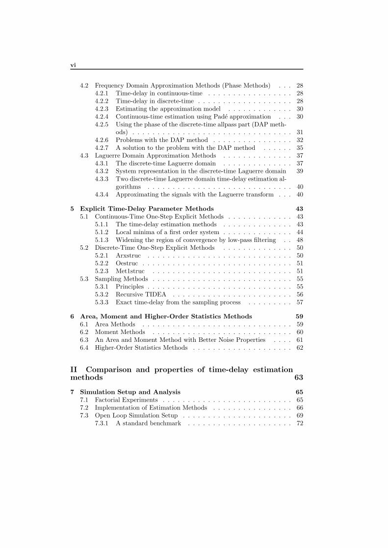
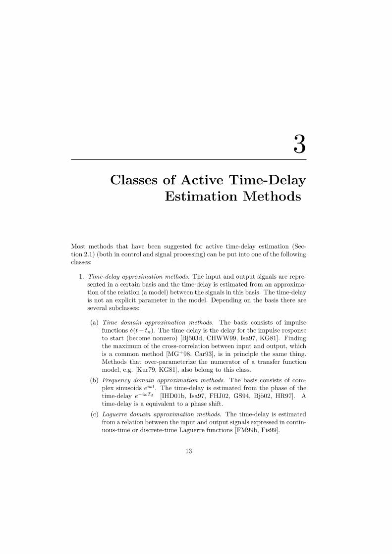
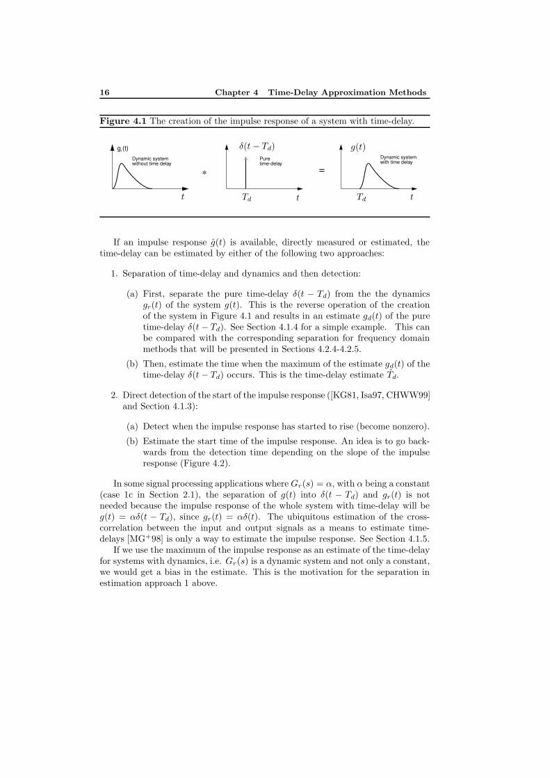
The impulse response of a system with time-delay is created as in Figure 4.1. Tothe left the impulse response gr(t) of the system without time-delay is depicted. Inthe middle the pure time-delay is seen as a system whose impulse response δ(t−Td)is an impulse at the time equal to the time-delay Td. To the right is the impulseresponse g(t) of the system with time-delay, which is the convolution of the twosystems to the left: g(t) = gr(t) ∗ δ(t− Td).
15
16 Chapter 4 Time-Delay Approximation Methods
Figure 4.1 The creation of the impulse response of a system with time-delay.
=*
gr (t)
Dynamic systemwithout time delay
Puretime-delay
Dynamic systemwith time delay
PSfrag replacements
ttt
u(t)y(t)s(t)
gts(t)
Td
TdTd
δ(t− Td) g(t)
gr(t)g(t)
If an impulse response g(t) is available, directly measured or estimated, thetime-delay can be estimated by either of the following two approaches:
1. Separation of time-delay and dynamics and then detection:
(a) First, separate the pure time-delay δ(t − Td) from the the dynamicsgr(t) of the system g(t). This is the reverse operation of the creationof the system in Figure 4.1 and results in an estimate gd(t) of the puretime-delay δ(t− Td). See Section 4.1.4 for a simple example. This canbe compared with the corresponding separation for frequency domainmethods that will be presented in Sections 4.2.4-4.2.5.
(b) Then, estimate the time when the maximum of the estimate gd(t) of thetime-delay δ(t− Td) occurs. This is the time-delay estimate Td.
2. Direct detection of the start of the impulse response ([KG81, Isa97, CHWW99]and Section 4.1.3):
(a) Detect when the impulse response has started to rise (become nonzero).
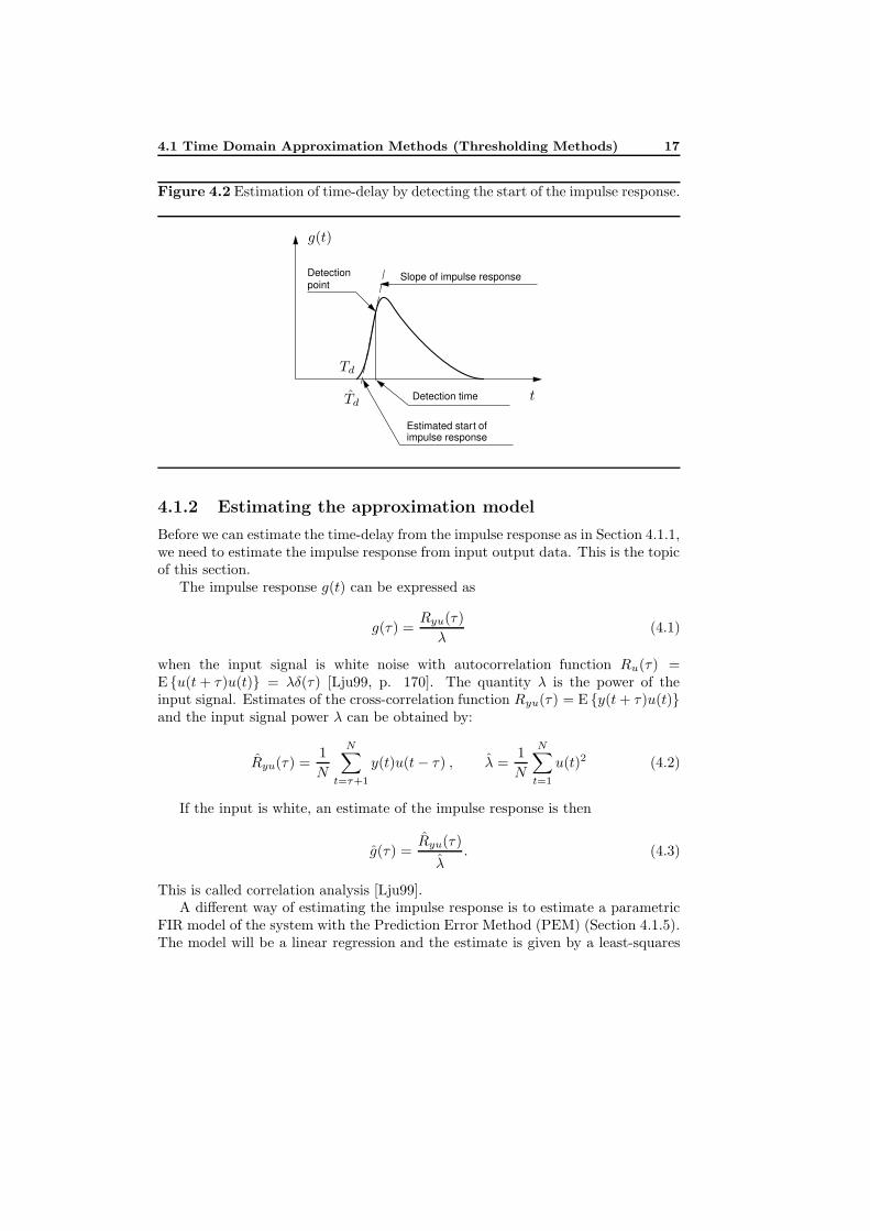
(b) Estimate the start time of the impulse response. An idea is to go back-wards from the detection time depending on the slope of the impulseresponse (Figure 4.2).
In some signal processing applications whereGr(s) = α, with α being a constant(case 1c in Section 2.1), the separation of g(t) into δ(t − Td) and gr(t) is notneeded because the impulse response of the whole system with time-delay will beg(t) = αδ(t − Td), since gr(t) = αδ(t). The ubiquitous estimation of the cross-correlation between the input and output signals as a means to estimate time-delays [MG+98] is only a way to estimate the impulse response. See Section 4.1.5.
If we use the maximum of the impulse response as an estimate of the time-delayfor systems with dynamics, i.e. Gr(s) is a dynamic system and not only a constant,we would get a bias in the estimate. This is the motivation for the separation inestimation approach 1 above.
4.1 Time Domain Approximation Methods (Thresholding Methods) 17
Figure 4.2 Estimation of time-delay by detecting the start of the impulse response.
Detectionpoint
Detection time
Estimated start ofimpulse response
Slope of impulse response
PSfrag replacements
t
u(t)y(t)s(t)
gts(t)
Td
Td
δ(t− Td) g(t)
gr(t)g(t)
4.1.2 Estimating the approximation model
Before we can estimate the time-delay from the impulse response as in Section 4.1.1,we need to estimate the impulse response from input output data. This is the topicof this section.
The impulse response g(t) can be expressed as
g(τ) =Ryu(τ)
λ(4.1)
when the input signal is white noise with autocorrelation function Ru(τ) =E {u(t+ τ)u(t)} = λδ(τ) [Lju99, p. 170]. The quantity λ is the power of theinput signal. Estimates of the cross-correlation function Ryu(τ) = E {y(t+ τ)u(t)}and the input signal power λ can be obtained by:
Ryu(τ) =1
N
N∑
t=τ+1
y(t)u(t− τ) , λ =1
N
N∑
t=1
u(t)2 (4.2)
If the input is white, an estimate of the impulse response is then
g(τ) =Ryu(τ)
λ. (4.3)
This is called correlation analysis [Lju99].A different way of estimating the impulse response is to estimate a parametric
FIR model of the system with the Prediction Error Method (PEM) (Section 4.1.5).The model will be a linear regression and the estimate is given by a least-squares
18 Chapter 4 Time-Delay Approximation Methods
estimate:
θN =
1
N
∑
t
ϕ(t)ϕ(t)T
︸ ︷︷ ︸
A
−1[1
N
∑
t
ϕ(t)y(t)
]
︸ ︷︷ ︸B
(4.4)
with ϕ(t) = [u(t), u(t − 1), ...] [Lju99, p. 204]. This is essentially the same asEquation (4.3). If the input signal u(t) is white, then the matrix A in Equation
(4.4) will be A = λ I and the matrix B will be
B =
Ryu(0)
Ryu(1)...
(4.5)
and θN =[g0 g1 . . .
]is the same as g(τ) =
[g0 g1 . . .
]=[
g(0) g(1) . . .]
in Equation (4.3).
The estimate θN will be Gaussian distributed when the noise is Gaussian. Evenif the noise is not Gaussian, θN will often be asymptotic Gaussian when N → ∞[Lju99, p. 556].
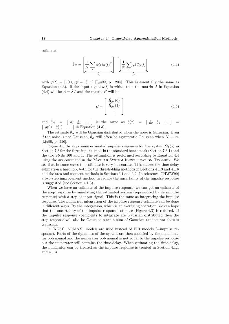
Figure 4.3 displays some estimated impulse responses for the system G1(s) inSection 7.3 for the three input signals in the standard benchmark (Section 7.3.1) andthe two SNRs 100 and 1. The estimation is performed according to Equation 4.4using the arx command in the Matlab System Identification Toolbox. Wesee that in some cases the estimate is very inaccurate. This makes the time-delayestimation a hard job, both for the thresholding methods in Sections 4.1.3 and 4.1.6and the area and moment methods in Sections 6.1 and 6.2. In reference [CHWW99]a two-step improvement method to reduce the uncertainty of the impulse responseis suggested (see Section 4.1.3).
When we have an estimate of the impulse response, we can get an estimate ofthe step response by simulating the estimated system (represented by its impulseresponse) with a step as input signal. This is the same as integrating the impulseresponse. The numerical integration of the impulse response estimate can be donein different ways. By the integration, which is an averaging operation, we can hopethat the uncertainty of the impulse response estimate (Figure 4.3) is reduced. Ifthe impulse response coefficients to integrate are Gaussian distributed then thestep response will also be Gaussian since a sum of Gaussian random variables isGaussian.
In [KG81], ARMAX models are used instead of FIR models (=impulse re-sponse). Parts of the dynamics of the system are then modeled by the denomina-tor polynomial and the numerator polynomial is not equal to the impulse responsebut the numerator still contains the time-delay. When estimating the time-delay,the numerator can be treated as the impulse response is treated in Section 4.1.1and 4.1.3.
4.1 Time Domain Approximation Methods (Thresholding Methods) 19
Figure 4.3 Impulse response estimate of the system G1 by the Matlab func-tion arx for different input signal types l and different SNRs ↔(Section 7.3). Noprewhitening of the input signal (Section 7.3). The solid line is the true impulseresponse. The circles are the estimated impulse response and the triangles mark±two estimated standard deviations. Note the different ranges of the vertical axes.(t130f1 SNR out))
0 10 20 30 40 50 60 70−0.02
0
0.02
0.04
0.06
0.08
Time [s]
Impulse response ,10−30%, SNR=100, G1
0 10 20 30 40 50 60 70−0.1
−0.05
0
0.05
0.1
0.15
Time [s]
Impulse response ,10−30%, SNR=1, G1
0 10 20 30 40 50 60 70−0.02
0
0.02
0.04
0.06
0.08
Time [s]
Impulse response ,0−100%, SNR=100, G1
0 10 20 30 40 50 60 70−0.05
0
0.05
0.1
0.15
Time [s]
Impulse response ,0−100%, SNR=1, G1
0 10 20 30 40 50 60 70−0.2
−0.1
0
0.1
0.2
0.3
Time [s]
Impulse response ,steps, SNR=100, G1
0 10 20 30 40 50 60 70−2
−1
0
1
2
Time [s]
Impulse response ,steps, SNR=1, G1
PSfrag replacements
tu(t)y(t)s(t)
gts(t)
TdTd
δ(t− Td)g(t)gr(t)g(t)
4.1.3 Estimating the start of the impulse response
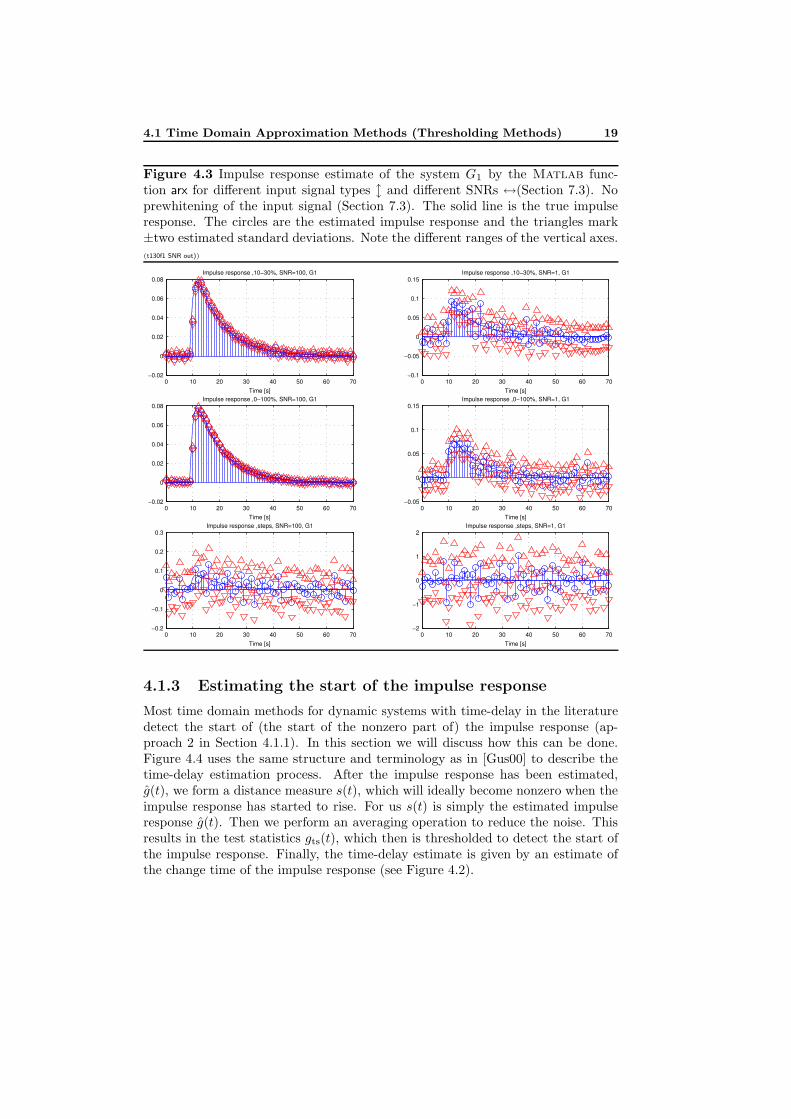
Most time domain methods for dynamic systems with time-delay in the literaturedetect the start of (the start of the nonzero part of) the impulse response (ap-proach 2 in Section 4.1.1). In this section we will discuss how this can be done.Figure 4.4 uses the same structure and terminology as in [Gus00] to describe thetime-delay estimation process. After the impulse response has been estimated,g(t), we form a distance measure s(t), which will ideally become nonzero when theimpulse response has started to rise. For us s(t) is simply the estimated impulseresponse g(t). Then we perform an averaging operation to reduce the noise. Thisresults in the test statistics gts(t), which then is thresholded to detect the start ofthe impulse response. Finally, the time-delay estimate is given by an estimate ofthe change time of the impulse response (see Figure 4.2).
20 Chapter 4 Time-Delay Approximation Methods
Figure 4.4 Steps in time-delay estimation in the time domain.
Impulseresponseestimation measure Averaging ThresholdDistance
Input output data Test statisticsTime-delayestimate
PSfrag replacements
t
u(t)
y(t) s(t) gts(t) Td
Tdδ(t− Td)
g(t)gr(t)
g(t)
The averaging to get the test statistics can be accomplished by one or several of:
Step response. Integration to step response.
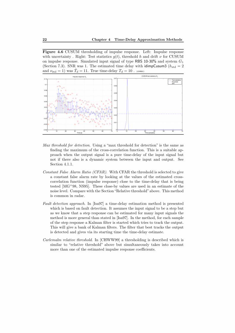
Cumulative sum (CUSUM). Perform an averaging of the estimated impulse or stepresponse by CUSUM [Pag54, Gus00, GLM01] before the thresholding. Thereare two user-selected parameters, the drift ν(t) and the threshold h(t). SeeAlgorithm 1. See Figure 4.6 for an example of CUSUM thresholding of animpulse response estimate.
Carlemalm impulse response. In [CHWW99] a special technique is used to decreasethe uncertainty of the estimated impulse response, cf. Figure 4.3. First, allcoefficients of the impulse response are estimated recursively by an LMS fil-ter [Gus00, GLM01]. Then these estimates are improved by one Kalman fil-ter [Gus00, GLM01] for each coefficient. The estimated coefficients from theLMS filter are used as measurement signals for the Kalman filters. The resultsfrom the Kalman filters are the second estimates of the coefficients (the firstestimates come from the LMS filter) and estimates of their covariance. Thistechnique requires white input and Gaussian noise.
Direct . Use the estimated estimated impulse or step response directly for thresh-olding. Using the impulse response directly is of course no averaging. SeeFigure 4.5 for an example of direct thresholding of a an impulse response esti-mate.
The thresholding (Figure 4.4) can be performed by:
Fixed threshold . The threshold is fixed and data independent.
Relative threshold . The threshold depends on the uncertainty of the impulse or stepresponse estimate. If we let the threshold be proportional to the uncertaintyof the impulse or step response estimate we will get a specified risk for falsealarm (saying that the time-delay is over when it is not). By lowering this risk(increasing the threshold) the probability of detection will also be lowered.
4.1 Time Domain Approximation Methods (Thresholding Methods) 21
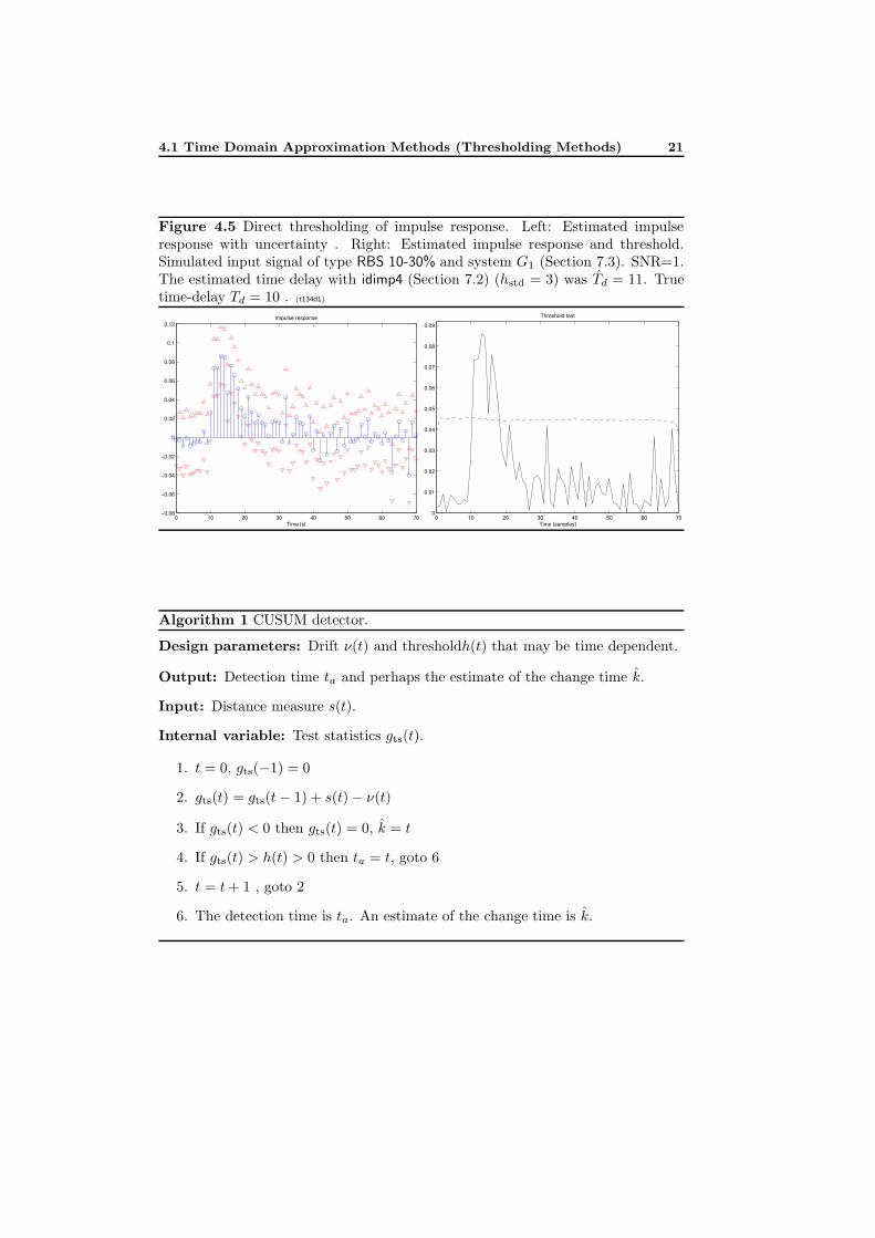
Figure 4.5 Direct thresholding of impulse response. Left: Estimated impulseresponse with uncertainty . Right: Estimated impulse response and threshold.Simulated input signal of type RBS 10-30% and system G1 (Section 7.3). SNR=1.The estimated time delay with idimp4 (Section 7.2) (hstd = 3) was Td = 11. Truetime-delay Td = 10 . (t134d1)
0 10 20 30 40 50 60 70−0.08
−0.06
−0.04
−0.02
0
0.02
0.04
0.06
0.08
0.1
0.12
Time [s]
Impulse response
PSfrag replacements
tu(t)y(t)s(t)
gts(t)
TdTd
δ(t− Td)g(t)gr(t)g(t)
0 10 20 30 40 50 60 700
0.01
0.02
0.03
0.04
0.05
0.06
0.07
0.08
0.09
Threshold test
Time [samples]
PSfrag replacements
tu(t)y(t)s(t)
gts(t)
TdTd
δ(t− Td)g(t)gr(t)g(t)
Algorithm 1 CUSUM detector.
Design parameters: Drift ν(t) and thresholdh(t) that may be time dependent.
Output: Detection time ta and perhaps the estimate of the change time k.
Input: Distance measure s(t).
Internal variable: Test statistics gts(t).
1. t = 0, gts(−1) = 0
2. gts(t) = gts(t− 1) + s(t)− ν(t)
3. If gts(t) < 0 then gts(t) = 0, k = t
4. If gts(t) > h(t) > 0 then ta = t, goto 6
5. t = t+ 1 , goto 2
6. The detection time is ta. An estimate of the change time is k.
22 Chapter 4 Time-Delay Approximation Methods
Figure 4.6 CUSUM thresholding of impulse response. Left: Impulse responsewith uncertainty . Right: Test statistics g(t), threshold h and drift ν for CUSUMon impulse response. Simulated input signal of type RBS 10-30% and system G1
(Section 7.3). SNR was 1. The estimated time delay with idimpCusum3 (hstd = 2and νstd = 1) was Td = 11. True time-delay Td = 10 . (t146b1)
0 10 20 30 40 50 60 70−0.06
−0.04
−0.02
0
0.02
0.04
0.06
0.08
0.1
0.12
Time [s]
Impulse response G1
PSfrag replacements
tu(t)y(t)s(t)
gts(t)
TdTd
δ(t− Td)g(t)gr(t)g(t)
0 10 20 30 40 50 60 700
0.01
0.02
0.03
0.04
0.05
0.06
0.07
CUSUM test statistics G1
Time [samples]
Test statisticsthreshold drift
PSfrag replacements
tu(t)y(t)s(t)
gts(t)
TdTd
δ(t− Td)g(t)gr(t)g(t)
Max threshold for detection. Using a “max threshold for detection” is the same asfinding the maximum of the cross-correlation function. This is a suitable ap-proach when the output signal is a pure time-delay of the input signal butnot if there also is a dynamic system between the input and output. SeeSection 4.1.1.
Constant False Alarm Ratio (CFAR). With CFAR the threshold is selected to givea constant false alarm rate by looking at the values of the estimated cross-correlation function (impulse response) close to the time-delay that is beingtested [MG+98, NS95]. These close-by values are used in an estimate of thenoise level. Compare with the Section“Relative threshold”above. This methodis common in radar.
Fault detection approach. In [Isa97] a time-delay estimation method is presentedwhich is based on fault detection. It assumes the input signal to be a step butas we know that a step response can be estimated for many input signals themethod is more general than stated in [Isa97]. In the method, for each sampleof the step response a Kalman filter is started which tries to track the output.This will give a bank of Kalman filters. The filter that best tracks the outputis detected and gives via its starting time the time-delay estimate.
Carlemalm relative threshold. In [CHWW99] a thresholding is described which issimilar to “relative threshold” above but simultaneously takes into accountmore than one of the estimated impulse response coefficients.
4.1 Time Domain Approximation Methods (Thresholding Methods) 23
Kurz detection. In [Kur79, KG81] the time-delay is estimated by detecting whenthe numerator coefficients of an estimated linear model no longer are zero. Dueto noise this is not easy and a special technique is used.
When a change in the estimated impulse response has been detected, the changetime can be estimated by going backwards from the detection time depending onthe slope of the impulse response (Figure 4.2). See [Gus00] for estimating thechange time when using CUSUM. In the simulations of thresholding methods inthis work the detection time and not an estimated change time was used as thetime-delay estimate. For example, in the CUSUM detection in Algorithm 1 thedetection time ta was uses as the time-delay estimate. This should cause bias as isdiscussed in Section 8.1.2.
4.1.4 Separating the time-delay and the dynamics
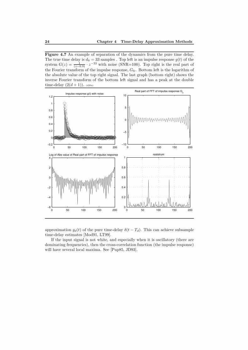
In this section we will give an example on how the dynamics can be separated fromthe time-delay (approach 1 in Section 4.1.1). We start with an impulse response ofa system with time-delay g(t) = gr(t) ∗ δ(t−Td) as in Section 4.1.1. See Figure 4.7(top left) for an example. The Fourier transform of g(t) is G(iω) = Gr(iω) ·e−iωTd .Then by taking the real part of G(iω) we get
Gfr(iω) = Re {G(iω)} = Re{Gr(iω) · eiωTd
}= Afr(iω) sin (Tdω + ϕ(iω)) ,
where
Afr(iω) =
√(ReGr(iω))2 + (ImGr(iω))2
ϕ(iω) = arcsin
(ReGr(iω)
Afr(iω)
).
The function Gfr(iω) consists of Afr(iω) which is modulated with a sinusoid with“frequency”Td and phase shift ϕ(iω) (Figure 4.7 (top right)). One idea to estimatethe “frequency” would be to study the “spectrum” of Gfr(iω). Since we alreadyare in the frequency domain, we could compute the inverse Fourier transform andlook for the peak at “frequency” Td. We see in Figure 4.7 (top right) that thereis an oscillation in Gfr(iω) but its amplitude is small. To increase the effect ofthe oscillation we take the logarithm (after taking the absolute value to avoid thelogarithm of negative values) which can be used to amplify weak parts of a positivesignal (Figure 4.7 (bottom left)). Finally, we compute the inverse Fourier transformand look for peaks at the “frequency” 2Td. Because the absolute value doubles thebase frequency of the periodic signal (the sinusoid) we need the number 2.
This method is similar to using cepstrum, in which we only take the absolutevalue instead of the absolute value of the real part as above, to find the time-delayof an echo [DC02, GLM01] (problems 1c and 2a in Section 2.1).
When a change in the estimated impulse response has been detected, the changetime can be estimated by taking the maximum of an interpolation of the estimated
24 Chapter 4 Time-Delay Approximation Methods
Figure 4.7 An example of separation of the dynamics from the pure time delay.The true time delay is d0 = 33 samples . Top left is an impulse response g(t) of thesystem G(z) = 1
(z−0.9) · z−33 with noise (SNR=100). Top right is the real part of
the Fourier transform of the impulse response, Gfr. Bottom left is the logarithm ofthe absolute value of the top right signal. The last graph (bottom right) shows theinverse Fourier transform of the bottom left signal and has a peak at the doubletime-delay (2(d+ 1)). (t237a)
0 50 100 150 200−0.2
0
0.2
0.4
0.6
0.8
1
1.2Impulse response g(t) with noise
PSfrag replacements
tu(t)y(t)s(t)
gts(t)
TdTd
δ(t− Td)g(t)gr(t)g(t)
0 50 100 150 200−10
−5
0
5
10
Real part of FFT of impulse response Gfr
PSfrag replacements
tu(t)y(t)s(t)
gts(t)
TdTd
δ(t− Td)g(t)gr(t)g(t)
0 50 100 150 200−6
−4
−2
0
2
4Log of Abs value of Real part of FFT of impulse response
PSfrag replacements
tu(t)y(t)s(t)
gts(t)
TdTd
δ(t− Td)g(t)gr(t)g(t)
0 50 100 150 2000
0.2
0.4
0.6
0.8
1realstrum
PSfrag replacements
tu(t)y(t)s(t)
gts(t)
TdTd
δ(t− Td)g(t)gr(t)g(t)
approximation gd(t) of the pure time-delay δ(t− Td). This can achieve subsampletime-delay estimates [Mod91, LT99].
If the input signal is not white, and especially when it is oscillatory (there aredominating frequencies), then the cross-correlation function (the impulse response)will have several local maxima. See [Pup85, JD93].
4.1 Time Domain Approximation Methods (Thresholding Methods) 25
4.1.5 Relation between PEM, cross-correlation, matched fil-ter and maximum likelihood estimation
In this section we will discuss the relation between the Prediction Error Method(PEM) [Lju99], cross-correlation method, matched filter [Han91] and maximumlikelihood estimation of the time-delay. The relation between PEM and correlationanalysis was shown in section 4.1.1. The relation between time-delay estimation inthe time and frequency domains is discussed in Section 4.2.2.
The prediction error method (PEM) is a fundamental approach to estimate
models of dynamic systems. In PEM the estimate θN of the model parametervector θ using N input output data is given (with a quadratic criterion) by
θN = arg minθ
1
N
N∑
t=1
1
2ε2(t|θ),
where ε2(t|θ) = y(t) − y(t|θ) is the prediction error of the model and y(t|θ) is theone-step prediction of the model output [Lju99]. If the data are generated by linear
systems and the model is linear, then θN will converge to
θ∗ = arg minθ
E
{1
2ε2(t|θ)
}
as the number of data N → ∞ [Lju99, Th.8.2, p.254]. The symbol E meansensemble averaging for stationary stochastic processes (statistical expectation) andtime averaging (as N → ∞) for deterministic signals. For all details of this resultsee [Lju99].
In the cross-correlation method for time-delay estimation, the original signalu(t) and the time-delayed signal y(t) are compared. They are put close to eachother. Then they are time-shifted until they agree the most. For stochastic pro-cesses this can more formally be written
d = arg maxτ
E {y(t)u(t− τ)} .
In reality this has to be implemented as
d = arg maxτ
∑
t
y(t)u(t− τ). (4.6)
The purpose of a matched filter [Han91] is to detect a known signal u(t). Thisis done by sending the received signal y(t) through a linear filter with the impulseresponse h(t) = u(−t). The filter is matched to the signal u(t). The output z(τ) (wehere use τ as the time variable instead of t) of the filter is given by the well-knownconvolution sum
z(τ) =∑
t
h(t− τ)y(t) =∑
τ
y(t)u(τ − t).
26 Chapter 4 Time-Delay Approximation Methods
The arrival time of the known signal can be estimated with the time when the filteroutput has its maximum value:
d = arg maxτ
z(τ) = arg maxτ
∑
τ
y(t)u(τ − t). (4.7)
As is seen, this is the same as the cross-correlation method for time-delay estimationin Equation (4.6).
We will now show the relation between the PEM and the cross-correlationmethod (matched filter) for a pure time-delay. We will show that for the activeTDE problem 1d in Section 2.1,
y(t) = u(t− d) + n(t) with n(t) white noise,
the prediction error method (PEM) in system identification and the matched filterare equivalent.
The PEM estimate uses the the one-step predictor y(t|τ) = u(t− τ) [Lju99] ofthe output signal y(t) for a pure time-delay of size τ . The PEM estimate is [Lju99]
d = arg minτ
∑(y(t|τ)− y(t))2 = arg min
τ
∑(u(t− τ) − y(t))2
= arg minτ
[∑u2(t− τ) +
∑y2(t)− 2
∑y(t)u(t− τ)
](4.8)
= arg minτ
[−2∑
y(t)u(t− τ)]
= arg maxτ
∑y(t)u(t− τ),
which is the same as the matched filter in Equation (4.7). The fourth equality signin (4.8) follows since
∑y2(t) does not contain τ and
∑u2(t − τ) =
∑u2(t) does
not depend on τ .In [JD93, p. 289] it is asserted that there is equivalence between maximum
likelihood estimation of the time-delay and a matched filter (cross-correlation) ifthe following assumptions are met:
• The active TDE problem 1d in Section 2.1 with discrete-time signals andtime-delay d:
y(t) = u(t− d) + n(t)
• The noise n(t) is Gaussian with rational spectrum with only poles but it isnot necessarily white.
• The duration of the input signal u(t) is short compared to the length of theobservation interval.
• The edge effects due to the finite observation interval are ignored.
The matched filter estimate is
d = arg maxτ
L−1∑
t=0
y(t)u(t− τ) (4.9)
4.1 Time Domain Approximation Methods (Thresholding Methods) 27
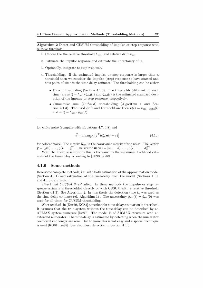
Algorithm 2 Direct and CUSUM thresholding of impulse or step response withrelative threshold.
1. Choose the the relative threshold hstd and relative drift νstd.
2. Estimate the impulse response and estimate the uncertainty of it.
3. Optionally, integrate to step response.
4. Thresholding. If the estimated impulse or step response is larger than athreshold then we consider the impulse (step) response to have started andthis point of time is the time-delay estimate. The thresholding can be either
• Direct thresholding (Section 4.1.3). The thresholds (different for eachtime) are h(t) = hstd · ystd(t) and ystd(t) is the estimated standard devi-ation of the impulse or step response, respectively.
• Cumulative sum (CUSUM) thresholding (Algorithm 1 and Sec-tion 4.1.3). The used drift and threshold are then ν(t) = νstd · ystd(t)and h(t) = hstd · ystd(t).
for white noise (compare with Equations 4.7, 4.8) and
d = arg maxτ
[yTR−1
nnu(t− τ)]
(4.10)
for colored noise. The matrix Rnn is the covariance matrix of the noise. The vectory = [y(0), . . . , y(L− 1)]T . The vector u(∆t) = [u(0− d), . . . , u(L− 1− d)]T .
With the above assumptions this is the same as the maximum likelihood esti-mate of the time-delay according to [JD93, p.289].
4.1.6 Some methods
Here some complete methods, i.e. with both estimation of the approximation model(Section 4.1.1) and estimation of the time-delay from the model (Sections 4.1.1and 4.1.3), are listed.
Direct and CUSUM thresholding. In these methods the impulse or step re-sponse estimate is thresholded directly or with CUSUM with a relative threshold(Section 4.1.3). See Algorithm 2. In this thesis the detection time ta was used asthe time-delay estimate (cf. Algorithm 1) . The uncertainty ystd(t) = ystd(0) wasused for all times for CUSUM thresholding.
Kurz method. In [Kur79, KG81] a method for time-delay estimation is described.It assumes that the true system without the time-delay can be described by anARMAX system structure [Isa97]. The model is of ARMAX structure with anextended numerator. The time-delay is estimated by detecting when the numeratorcoefficients no longer are zero. Due to noise this is not easy and a special techniqueis used [KG81, Isa97]. See also Kurz detection in Section 4.1.3.
28 Chapter 4 Time-Delay Approximation Methods
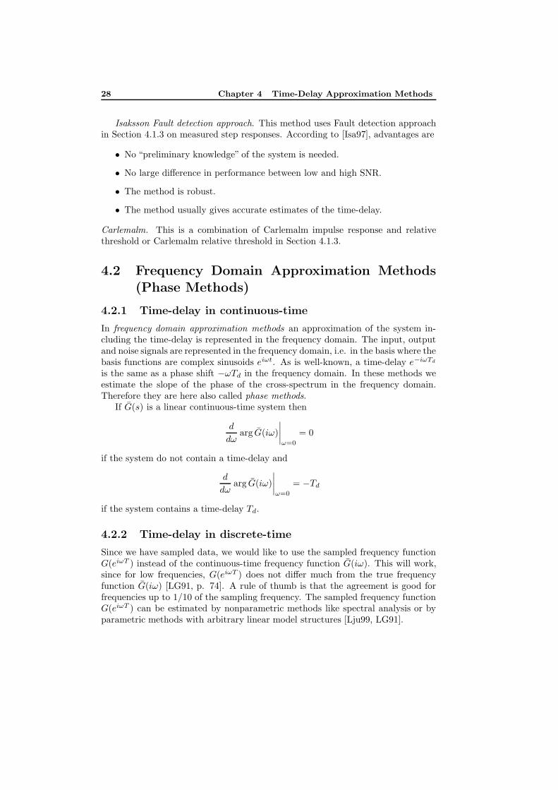
Isaksson Fault detection approach. This method uses Fault detection approachin Section 4.1.3 on measured step responses. According to [Isa97], advantages are
• No “preliminary knowledge” of the system is needed.
• No large difference in performance between low and high SNR.
• The method is robust.
• The method usually gives accurate estimates of the time-delay.
Carlemalm. This is a combination of Carlemalm impulse response and relativethreshold or Carlemalm relative threshold in Section 4.1.3.
4.2 Frequency Domain Approximation Methods(Phase Methods)
4.2.1 Time-delay in continuous-time
In frequency domain approximation methods an approximation of the system in-cluding the time-delay is represented in the frequency domain. The input, outputand noise signals are represented in the frequency domain, i.e. in the basis where thebasis functions are complex sinusoids eiωt. As is well-known, a time-delay e−iωTd
is the same as a phase shift −ωTd in the frequency domain. In these methods weestimate the slope of the phase of the cross-spectrum in the frequency domain.Therefore they are here also called phase methods.
If G(s) is a linear continuous-time system then
d
dωarg G(iω)
∣∣∣∣ω=0
= 0
if the system do not contain a time-delay and
d
dωarg G(iω)
∣∣∣∣ω=0
= −Td
if the system contains a time-delay Td.
4.2.2 Time-delay in discrete-time
Since we have sampled data, we would like to use the sampled frequency functionG(eiωT ) instead of the continuous-time frequency function G(iω). This will work,since for low frequencies, G(eiωT ) does not differ much from the true frequencyfunction G(iω) [LG91, p. 74]. A rule of thumb is that the agreement is good forfrequencies up to 1/10 of the sampling frequency. The sampled frequency functionG(eiωT ) can be estimated by nonparametric methods like spectral analysis or byparametric methods with arbitrary linear model structures [Lju99, LG91].
4.2 Frequency Domain Approximation Methods (Phase Methods) 29
In time-delay estimation by spectral analysis, we utilize the formula [GLM01]Φyu(ω) = G(eiωT )Φu(ω) or
G(eiωT ) =Φyu(ω)
Φu(ω), (4.11)
where the sampled frequency function G(eiωT ) is connected with the cross-spectrumΦyu(ω) between output y(t) and input u(t) and the (auto) spectrum Φu(ω) of theinput. A natural estimate of G(eiωT ) is then to use the estimated cross-spectrumΦyu(ω) divided by the estimated (auto) spectrum Φu(ω):
G(eiωT ) =Φyu(ω)
Φu(ω). (4.12)
The cross-spectrum and the (auto) spectrum can be estimated in different ways.Normally, the start is the periodogram [GLM01, Lju99]. Then it is smoothed withsome method [GLM01, Lju99, Wik02].
In [HR95, HR97, Wik02] the cross-spectrum is then noise reduced by windowingin the time domain before returning to the frequency domain. This is possible forwideband signals whose cross-correlation function in the time domain is narrow.
Then the phase of G(eiωT ) is studied to give an estimate of the time-delay
Td = − d
dωarg G(eiωT )
∣∣∣∣ω=0
where the derivative is approximated in a suitable way. The reference [Hor00,IHD01b] contains an approximation of the derivative for the active TDE prob-lem (2.2). The derivative is easier to approximate for the passive TDE problem 2a(Section 2.1) because then the time-delay is the only thing that affects the phase.See [Wik02] for an example of approximation of the derivative in this case.
Time-delay estimation by spectral analysis is equivalent to time-delay esti-mation by cross-correlation analysis in the frequency domain. Since the cross-spectrum Φyu(ω) is the discrete-time Fourier transform of the cross-correlationfunction Ryu(τ) [GLM01, p. 54],
Φyu(ω) = Ts
∞∑
k=−∞Ryu(k)eiωkTs ,
and in the same way the autospectrum the Fourier transform of the autocorrelationfunction Ru(τ), we see that Equation (4.12) is the same as Equation (4.1) in thefrequency domain (if the input signal is white). In the time domain (Equation (4.1))a time-delay in the system will be a time-delay in h(τ). In the frequency domain(Equation (4.12)) a time-delay in the system will be a phase shift in G(eiωT ). Foran example of time-delay estimation by nonparametric methods see [Wik02].
If the model structure in a parametric method is a linear regression then themodel can be estimated by cross- and autocorrelations. Compare with the FIRmodel in Section 4.1.2. For some examples of time-delay estimation by parametricmethods see [Hor00, IHD01b, Bjo02].
30 Chapter 4 Time-Delay Approximation Methods
4.2.3 Estimating the approximation model
To use the estimation methods in the previous section we first must estimate adiscrete-time model of the true system with time-delay. One interesting modelstructure to use is the Laguerre model structure. In this section we briefly describethis structure.
If a discrete-time system G(z) is is strictly proper, asymptotically stable andcontinuous in |z| ≥ 1, then it can be written [Wah91, p. 552]:
G(z) =
∞∑
k=1
dk
√(1− α2)Tsz − α
(1− αzz − α
)k−1
=
∞∑
k=1
dkLk(z) (4.13)
with |z| ≥ 1 and −1 < α < 1. Ts is the sampling interval and dk are somecoefficients. We change from the Z-transform variable z to the delay operator qand write the functions Lk(z) as
Lk(q) =
√(1− α2)Tsq
−1
1− αq−1
(−α+ q−1
1− αq−1
)k−1
. (4.14)
These functions are called the discrete-time Laguerre functions in the frequencydomain.
A model with a finite number of Laguerre functions looks like
y(t) = G(q)u(t) + v(t) (4.15)
G(q) =
nlag∑
k=1
dkLk(q) (4.16)
with y(t), u(t) and v(t) being the output, input and noise signals respectively. Themodel G(q) is an approximation of the true system G(z) in Equation (4.13).
In [Hor00, IHD01b] a Laguerre model was used. There is, however, nothing thatprevents us from using a model of a different structure and estimate the time-delayfrom it. For example, FIR, ARX or output error (OE) model structures [Lju99]could be used. We will see examples on this later.
4.2.4 Continuous-time estimation using Pade approximation
A time-delay e−sTd can be approximated by a Pade approximation of the first order(see for example [Mat96, GLM01, Isa97, p. 149])
e−sTd ≈ 1− sTd/21 + sTd/2
= H1(s) (4.17)
for small |sTd|.
4.2 Frequency Domain Approximation Methods (Phase Methods) 31
The amplitude of both the time-delay e−iωTd and the all-pass system H1(s) isequal to one. It is the phase that characterizes the time-delay and it is desirable thatthe all-pass system approximates this well. Pade approximations of time-delays ofhigher orders are also possible [Lam93, eq. (2.1) and (2.2)], [Isa97] or in [GVL96,p.572]. All zeros in a Pade approximation are non-minimum-phase [Isa97].
An approach to estimate the time-delay from a Pade approximation was de-scribed in [Isa97]. After the discrete-time Laguerre model has been estimated, itszeros are converted to continuous-time by means of
si ≈1
Tslog(zi) (4.18)
This approximation is valid when the sampling period Ts → 0 and the order n ofthe numerator polynomial and the order m of the denominator polynomial of thecontinuous-time system fulfills n+ 1 = m [ASH84]. .
Let the true continuous-time system be G(s) = G1(s) · e−sTd = G1(s) · Gap(s).We assume that all non-minimum-phase zeros originate from the time-delay andnot from the remaining system G1(s). The system G1(s) is thus assumed to beminimum-phase. By comparing the non-minimum-phase zeros with the zeros of anPade´ approximation, the time-delay can be decided from [Isa97] as
Td2
=∑
RHP
1
si, (4.19)
where RHP means Right Half Plane.The time-delay estimate in number of sampling intervals is [Isa97, Hor00]
k =TdTs
+ 1 (4.20)
The number 1 in Equation (4.20) is added to give the time-delay after samplingsince zero-order-hold sampling gives an extra time-delay of one sampling interval.
A problem with this method is that it can deliver complex valued time-delayestimates.
4.2.5 Using the phase of the discrete-time allpass part (DAPmethods)
Assume the true continuous-time system is G(s) = G1(s) · e−sTd = G1(s) · Gap(s).The system G1(s) is linear and time invariant. Gap(s) is the time-delay. Weestimate a discrete-time rational linear model G(z) of G(s) and factorizeG(z) into aminimum-phase system G1(z) and an allpass system Gap(z): G(z) = G1(z)Gap(z).(Allpass means
∣∣Gap(eiω)∣∣ ≡ 1) We then consider Gap(e
iωTs) as an approximationof the time-delay Gap(iω) = e−iωTd [Hor00, IHD01b]. A pure time-delay is ofcourse an allpass system. We get the allpass part Gap(z) of G(z) if we put all non-minimum phase (outside the unit circle) zeros of G(z) into Gap(z) and add polesto Gap(z) which are the non-minimum phase zeros mirrored in the unit circle.
32 Chapter 4 Time-Delay Approximation Methods
If we approximate a continuous-time linear system Gap(s) with a discrete-time linear system Gap(z) by sampling, then the frequency functions Gap(iω) andGap(e
iωTs) will agree well for low frequencies [GL97, p. 115-116]. [GL97] has therule-of-thumb that frequencies up to 1/10 of the sampling frequency gives a goodagreement.
From the allpass model Gap(eiωTs) the time-delay can be estimated by taking
the derivative of the phase ϕ(ω) = argGap(eiωTs). The motivation for this is that
the time-delay of the true system is given in this way:
dϕ
dω=d arg Gap(iω)
dω=
d
dωarg e−iωTd=
d
dω{−ωTd} = −Td (4.21)
Our time-delay estimate Td is given by an approximation of the derivative of thephase ϕ(ωTs) = argGap(e
iωTs):
Td ≈ −ϕ(ω1Ts)
ω1Ts= −argGap(e
iω1Ts)
ω1Ts(4.22)
for a small ω1 and adding a 1 because of the extra time-delay that is created bythe sampling:
Td = −argGap(eiω1Ts)
ω1Ts+ 1; ω1 small (4.23)
This approach is described in [Hor00, IHD01b]. (In [Hor00, IHD01b] a differentderivation is done.) In [Hor00, IHD01b] ω1 = 10−4 is suggested. The method inEquation 4.23 is in this thesis called DAP (Discrete-time Allpass Phase). Otherforms of approximations of the derivative should also be possible.
4.2.6 Problems with the DAP method
In order to better understand how the DAP method works, we will in this sectionin detail calculate the DAP estimate l for two simulated trials. In one of the trialsthe method will work well but in the other it will fail completely.
By looking at how the phase of a model G(eiωTs) can be calculated from thepoles and zeros of G(z) we can get some insight into what happens in the calculationof the time-delay estimate in Equation (4.23).
If we have a rational discrete-time transfer function
G(z) = β(z − z1) . . . (z − zm)
(z − p1) . . . (z − pn), (4.24)
its frequency function will be
G(eiωTs) = β(eiωTs − z1) . . . (eiω − zm)
(eiωTs − p1) . . . (eiωTs − pn). (4.25)
Let Zk(ω) be the vector (eiωTs − zk) from zk to the point eiωTs on the unit circle.Write Zk(ω) in polar form as Zk(ω) = Zk(ω)eiψk(ω), where Zk(ω) is the absolute
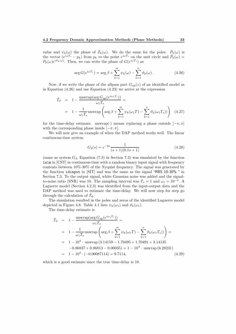
4.2 Frequency Domain Approximation Methods (Phase Methods) 33
value and ψk(ω) the phase of Zk(ω). We do the same for the poles. Pk(ω) isthe vector (eiωTs − pk) from pk to the point eiωTs on the unit circle and Pk(ω) =Pk(ω)eiϑk(ω). Then, we can write the phase of G(eiωTs) as
argG(eiωTs) = argβ +
m∑
k=1
ψk(ω)−n∑
k=1
ϑk(ω). (4.26)
Now, if we write the phase of the allpass part Gap(z) of an identified model asin Equation (4.26) and use Equation (4.23) we arrive at the expression
Td = 1− unwrap(argGap(eiω1Ts))
ω1Ts=
= 1− 1
ω1Tsunwrap
(argβ +
m∑
k=1
ψk(ω1T )−n∑
k=1
ϑk(ω1Ts))
)(4.27)
for the time-delay estimate. unwrap(·) means replacing a phase outside [−π, π]with the corresponding phase inside [−π, π].
We will now give an example of when the DAP method works well. The linearcontinuous-time system
G2(s) = e−9s 1
(s+ 1)(0.1s+ 1)(4.28)
(same as system G2, Equation (7.3) in Section 7.3) was simulated by the functionlsim in [CST] in continuous-time with a random binary input signal with frequencycontents between 10%-30% of the Nyquist frequency. The signal was generated bythe function idinput in [SIT] and was the same as the signal “RBS 10-30% ” inSection 7.3. To the output signal, white Gaussian noise was added and the signal-to-noise ratio (SNR) was 10. The sampling interval was Ts = 1 and ω1 = 10−4. ALaguerre model (Section 4.2.3) was identified from the input-output data and theDAP method was used to estimate the time-delay. We will now step for step gothrough the calculation of Td.
The simulation resulted in the poles and zeros of the identified Laguerre modeldepicted in Figure 4.8. Table 4.1 lists ψk(ω1) and ϑk(ω1).
The time-delay estimate is
Td = 1− unwrap(argGap(eiω1Ts))
ω1Ts=
= 1− 1
ω1Tsunwrap
(argβ +
m∑
k=1
ψk(ω1T )−n∑
k=1
ϑk(ω1Ts))
)=
= 1− 104 · unwrap (3.14159− 1.70495 + 1.70491 + 3.14135
−0.86837 + 0.86813− 0.00035) = 1− 104 · unwrap (6.28231)
= 1− 104 · (−0.00087114) = 9.7114, (4.29)
which is a good estimate since the true time-delay is 10.
34 Chapter 4 Time-Delay Approximation Methods
Table 4.1 ψk(ω1) and ϑk(ω1) in Equation (4.26) for ω1 = 10−4 for the successfulestimation (left,argβ = 3.14159), the failed estimation (middle, argβ = 0, not thesame estimated model as for the successful estimate) and after removing the realzero just outside the unit circle (right, argβ = 3.14159, the same estimated modelas for the failed estimate).
Successful estimation Failed estimation After zero guarding
ψk(ω1) ϑk(ω1) ψk(ω1) ϑk(ω1) ψk(ω1) ϑk(ω1)
-1.70495 0.86837 -1.71186 0.84682 -1.71186 0.846821.70491 -0.86813 1.71182 -0.84658 1.71182 -0.846583.14135 0.000347 3.14125 0.000445 3.14125 0.000445
3.07613 0.06556
Figure 4.8 Pole-zero plots of two identified Laguerre models. System G2 and inputsignal RBS 10-30% (Section 7.3). SNR =10. No prewhitening (Section 7.3) or zeroguarding (Section 4.2.7). The poles of the models should all be located at α = 0.8but due to well-known numerical problems with multiple poles they are somewhatspread. Left plot: Successful time-delay estimation (Td = 9.7114). Right plot:Failing time-delay estimation (Td = 1321.86). This simulation was one of only 3out of 1024 simulations with failing time-delay estimation for SNR = 10. With alower SNR the percentage of failing estimations is much higher. See Section 4.2.7.(t122a1)
Real Axis
Imag
Axi
s
Pole−zero map
0.5 1 1.5−0.8
−0.6
−0.4
−0.2
0
0.2
0.4
0.6
0.8Pzmap whole model, t122b1, Trial 3
PSfrag replacements
tu(t)y(t)s(t)
gts(t)
TdTd
δ(t− Td)g(t)gr(t)g(t)
a. Successful
Real Axis
Imag
Axi
s
Pole−zero map
0.5 1 1.5−0.8
−0.6
−0.4
−0.2
0
0.2
0.4
0.6
0.8Pzmap whole model, t122a1, Trial 941, Sys 2
PSfrag replacements
tu(t)y(t)s(t)
gts(t)
TdTd
δ(t− Td)g(t)gr(t)g(t)
b. Failing
4.2 Frequency Domain Approximation Methods (Phase Methods) 35
We will now study a case when the time-delay estimation fails. The only differ-ence to the successful trial in the simulation setup is a different noise realization.The zeros and poles of the identified Laguerre model are shown in Figure 4.8. Wenote that the zero on the real axis just inside the unit circle in the successful simu-lation has moved to just outside the unit circle. We will later see what impact thiswill have on the time-delay estimate. Table 4.1 lists ψk(ω1) and ϑk(ω1).
The time-delay estimate will now be
Td = 1− unwrap(argGap(eiω1Ts))
ω1Ts=
= 1− 1
ω1Tsunwrap
(argβ +
m∑
k=1
ψk(ω1T )−n∑
k=1
ϑk(ω1Ts))
)=
= 1− 104 · unwrap (0− 1.71186 + 1.71182 + 3.14125 + 3.07613
−0.84682 + 0.8465− 0.000445− 0.06556) =
1− 104 · unwrap (6.1511) = 1− 104 · (−0.132086) = 1321.9. (4.30)
As can be seen, the estimate is completely wrong.
4.2.7 A solution to the problem with the DAP method
As already mentioned in the previous section, a difference between the identifiedmodels in the successful and the failing trials was that the zero on the real axis justinside the unit circle in the successful trial had moved to outside the unit circle.Let us see what happens if we simply remove the moved zero from the model withthe failing estimate. This results in the ψk(ω1) and ϑk(ω1) in Table 4.1. Theremaining ψk(ω1) and ϑk(ω1) values in Table 4.1 are similar to the ones for thesuccessful estimation in Table 4.1.
The time-delay estimate will now be
Td = 1− unwrap(argGap(eiω1Ts))
ω1Ts=
= 1− 1
ω1Tsunwrap
(argβ +
m∑
k=1
ψk(ω1T )−n∑
k=1
ϑk(ω1Ts))
)=
= 1− 104 · unwrap (3.14159− 1.71186 + 1.71182 + 3.14125
−0.84682 + 0.84658− 0.000445) = 1− 104 · unwrap (6.28212)
= 1− 104 · (−0.00106586) = 11.6586, (4.31)
which is an acceptable estimate. It is much better than in Section 4.2.6 with thefailing estimation. It seems like the only significant difference between the modelswith successful and failing estimation is if a certain zero is inside or outside theunit circle.
We will now study the uncertainty in the zeros and the time-delay estimate.We note in Equation (4.26) that if we move a zero from inside to outside of the
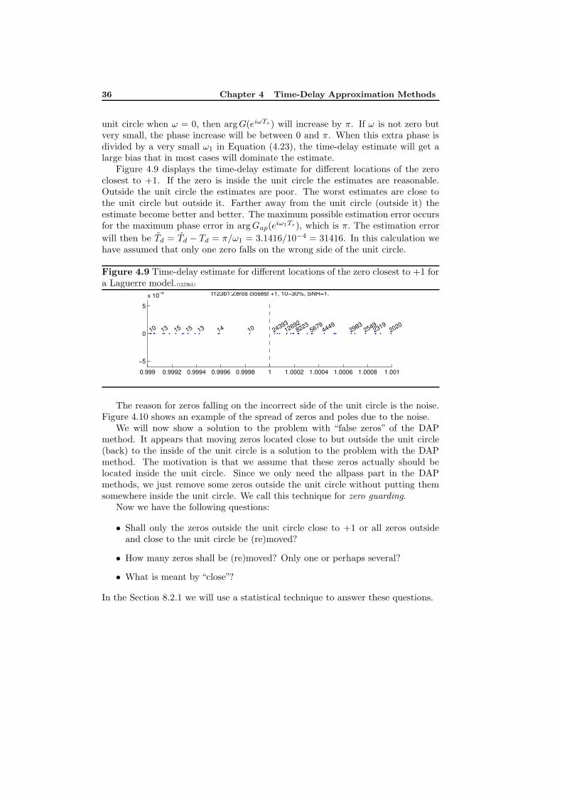
36 Chapter 4 Time-Delay Approximation Methods
unit circle when ω = 0, then argG(eiωTs) will increase by π. If ω is not zero butvery small, the phase increase will be between 0 and π. When this extra phase isdivided by a very small ω1 in Equation (4.23), the time-delay estimate will get alarge bias that in most cases will dominate the estimate.
Figure 4.9 displays the time-delay estimate for different locations of the zeroclosest to +1. If the zero is inside the unit circle the estimates are reasonable.Outside the unit circle the estimates are poor. The worst estimates are close tothe unit circle but outside it. Farther away from the unit circle (outside it) theestimate become better and better. The maximum possible estimation error occursfor the maximum phase error in argGap(e
iω1Ts), which is π. The estimation error
will then be Td = Td − Td = π/ω1 = 3.1416/10−4 = 31416. In this calculation wehave assumed that only one zero falls on the wrong side of the unit circle.
Figure 4.9 Time-delay estimate for different locations of the zero closest to +1 fora Laguerre model.(t123b1)
0.999 0.9992 0.9994 0.9996 0.9998 1 1.0002 1.0004 1.0006 1.0008 1.001
−5
0
5
x 10−6
298315 24393
10 567914 2549
202015 12692
822313 13 2319
10 4449
t123b1:Zeros closest +1, 10−30%, SNR=1.
PSfrag replacements
tu(t)y(t)s(t)
gts(t)
TdTd
δ(t− Td)g(t)gr(t)g(t)
The reason for zeros falling on the incorrect side of the unit circle is the noise.Figure 4.10 shows an example of the spread of zeros and poles due to the noise.
We will now show a solution to the problem with “false zeros” of the DAPmethod. It appears that moving zeros located close to but outside the unit circle(back) to the inside of the unit circle is a solution to the problem with the DAPmethod. The motivation is that we assume that these zeros actually should belocated inside the unit circle. Since we only need the allpass part in the DAPmethods, we just remove some zeros outside the unit circle without putting themsomewhere inside the unit circle. We call this technique for zero guarding.
Now we have the following questions:
• Shall only the zeros outside the unit circle close to +1 or all zeros outsideand close to the unit circle be (re)moved?
• How many zeros shall be (re)moved? Only one or perhaps several?
• What is meant by “close”?
In the Section 8.2.1 we will use a statistical technique to answer these questions.
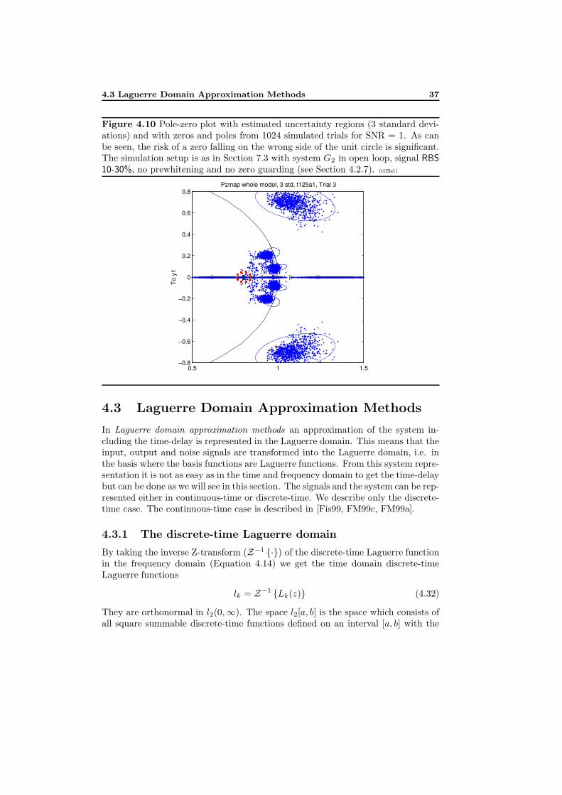
4.3 Laguerre Domain Approximation Methods 37
Figure 4.10 Pole-zero plot with estimated uncertainty regions (3 standard devi-ations) and with zeros and poles from 1024 simulated trials for SNR = 1. As canbe seen, the risk of a zero falling on the wrong side of the unit circle is significant.The simulation setup is as in Section 7.3 with system G2 in open loop, signal RBS10-30%, no prewhitening and no zero guarding (see Section 4.2.7). (t125a1)
0.5 1 1.5−0.8
−0.6
−0.4
−0.2
0
0.2
0.4
0.6
0.8Pzmap whole model, 3 std, t125a1, Trial 3
To y
1
PSfrag replacements
tu(t)y(t)s(t)
gts(t)
TdTd
δ(t− Td)g(t)gr(t)g(t)
4.3 Laguerre Domain Approximation Methods
In Laguerre domain approximation methods an approximation of the system in-cluding the time-delay is represented in the Laguerre domain. This means that theinput, output and noise signals are transformed into the Laguerre domain, i.e. inthe basis where the basis functions are Laguerre functions. From this system repre-sentation it is not as easy as in the time and frequency domain to get the time-delaybut can be done as we will see in this section. The signals and the system can be rep-resented either in continuous-time or discrete-time. We describe only the discrete-time case. The continuous-time case is described in [Fis99, FM99c, FM99a].
4.3.1 The discrete-time Laguerre domain
By taking the inverse Z-transform (Z−1 {·}) of the discrete-time Laguerre functionin the frequency domain (Equation 4.14) we get the time domain discrete-timeLaguerre functions
lk = Z−1 {Lk(z)} (4.32)
They are orthonormal in l2(0,∞). The space l2[a, b] is the space which consists ofall square summable discrete-time functions defined on an interval [a, b] with the
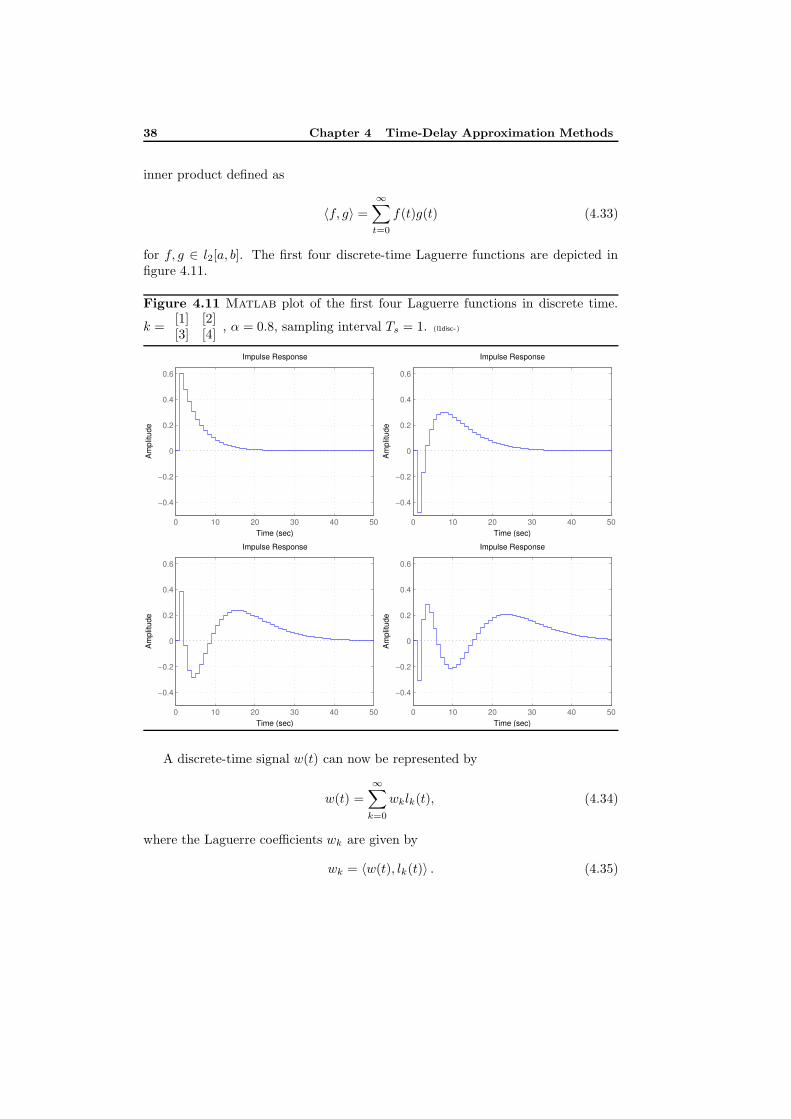
38 Chapter 4 Time-Delay Approximation Methods
inner product defined as
〈f, g〉 =
∞∑
t=0
f(t)g(t) (4.33)
for f, g ∈ l2[a, b]. The first four discrete-time Laguerre functions are depicted infigure 4.11.
Figure 4.11 Matlab plot of the first four Laguerre functions in discrete time.
k =[1] [2][3] [4]
, α = 0.8, sampling interval Ts = 1. (l1disc-)
Impulse Response
Time (sec)
Am
plitu
de
0 10 20 30 40 50
−0.4
−0.2
0
0.2
0.4
0.6
PSfrag replacements
tu(t)y(t)s(t)
gts(t)
TdTd
δ(t− Td)g(t)gr(t)g(t)
Impulse Response
Time (sec)
Am
plitu
de
0 10 20 30 40 50
−0.4
−0.2
0
0.2
0.4
0.6
PSfrag replacements
tu(t)y(t)s(t)
gts(t)
TdTd
δ(t− Td)g(t)gr(t)g(t)
Impulse Response
Time (sec)
Am
plitu
de
0 10 20 30 40 50
−0.4
−0.2
0
0.2
0.4
0.6
PSfrag replacements
tu(t)y(t)s(t)
gts(t)
TdTd
δ(t− Td)g(t)gr(t)g(t)
Impulse Response
Time (sec)
Am
plitu
de
0 10 20 30 40 50
−0.4
−0.2
0
0.2
0.4
0.6
PSfrag replacements
tu(t)y(t)s(t)
gts(t)
TdTd
δ(t− Td)g(t)gr(t)g(t)
A discrete-time signal w(t) can now be represented by
w(t) =
∞∑
k=0
wklk(t), (4.34)
where the Laguerre coefficients wk are given by
wk = 〈w(t), lk(t)〉 . (4.35)
4.3 Laguerre Domain Approximation Methods 39
This means that the coefficients wk describe (linearly) independent properties ofthe signal w(t). Since all real signals have finite extent in the time, they belong tol2 (for discrete-time) and can therefore be represented exactly by an infinite sumas in Equations (4.34)-(4.35).
4.3.2 System representation in the discrete-time Laguerredomain
For the discrete-time signal model
y(t) = u(t− d) + n(t),
where t and d only can be integer valued [Fis99], the relation between the input,output and noise signals in the discrete-time Laguerre domain is [Fis99, FM99c]
yk =
k∑
l=0
φk,lul + nk, (4.36)
where yk, ul and nk are the Laguerre coefficients for the output, input and noisesignals, respectively. Thus, the relation between the input and the output in theLaguerre domain can be seen as a time-varying linear filter. The time-varyingimpulse response φk,l is given by [Fis99, FM99c]
φk,l = 〈GLl , Lk〉 , (4.37)
where G = G(z) = z−d and 〈·, ·〉 is the scalar product in the Z domain [FM99b].The relation in Equation (4.36) can be rewritten as a linear regression [Fis99,
FM99c, FM99b]
yk = ϕTk Θ + nk, (4.38)
with the regression vector ϕk = [ϕk,1, . . . , ϕk,N+1]T , whose elements are
ϕk,1 = u0
ϕk,l+1 = (1−α2)l
l!(l−1)!
∑k−lm=0(−1)k+l−mαk−2l−m (k−m−1)!
(k−m−l)! um, k ≥ l > 0
ϕk,l+1 = 0 N ≥ l > k
(4.39)
N + 1 is the total number of Laguerre coefficients and α is the Laguerre pole(Equation 4.14). The parameter vector Θ is [FM99b]
Θ =[
1, d, . . . , d(d− 1) · · · (d− (N − 1))]Tαd. (4.40)
Here it is seen where the time-delay Td comes in.In [Fis99, FM99c] a method to estimate the time-delay is suggested: Let
Y = [y0, . . . , yN ]T (4.41)
40 Chapter 4 Time-Delay Approximation Methods
and
Φ = [ϕ0, . . . , ϕN ]T . (4.42)
Since Φ is a square nonsingular matrix, Θ could be estimated by
Θ = Φ−1Y. (4.43)
d =(1T1
)−11TYd =
1
N1T D +
N − 1
2, (4.44)
where 1 = [1, . . . , 1]T , Yd = D + [0, 1, . . . , N − 1]T and D = diag(
Θ)†
Θ. The
vector Θ is given by the vector Θ without the last element and Θ by Θ withoutthe first element. The symbol † means pseudoinverse. In [FM99b] also an othermethod to estimate the time-delay is suggested. See also the next section.
4.3.3 Two discrete-time Laguerre domain time-delay estima-tion algorithms
In [Fis99, FM99c, FM99b] two algorithms for the implementation of time-delayestimation based on the system representation (4.38), (4.39)-(4.40) in the discrete-time Laguerre domain are given. One of them uses Equation (4.44). They alsohave some features to enhance the numerical properties.
The matrix Φ will not be well-conditioned for large N [Fis99]. The numericalproperties of Φ are improved by using SVD (singular value decomposition [HJ91]) toextract the most significant part of Φ. See [Fis99, FM99a, FM99b] for details. Thenumber of singular values (the largest ones) to retain is a user-defined parameter.It is in this thesis set to 5, which is chosen after some simple tests.
The time-delay d can be estimated in two ways, here called tausvd and taulp1.In tausvd, d is estimated by least squares as in Equation (4.44). In taulp1 theΘ estimate (Equation (4.43)) is further improved by an iterative algorithm calledMIRLS (Modified Iteratively Reweighted Least Squares) [FM99b, CCS94] beforeestimating the time-delay by Equation (4.44). See Algorithms 3-4.
Several parameters must be selected by the user, most importantly the Laguerrepole α and the number N + 1 of Laguerre functions to use. These must be selectedto suit the input and output signals and the available execution time [Fis99, FM99c,FM99b, Bjo03e].
It is also possible to use approximation methods in other domains, e.g. theKautz domain [Kau54, Wah94, SBS97].
4.3.4 Approximating the signals with the Laguerre trans-form
A necessary condition for the Laguerre domain approximation estimation methodsto be successful is that the input and output signals can be represented accurately
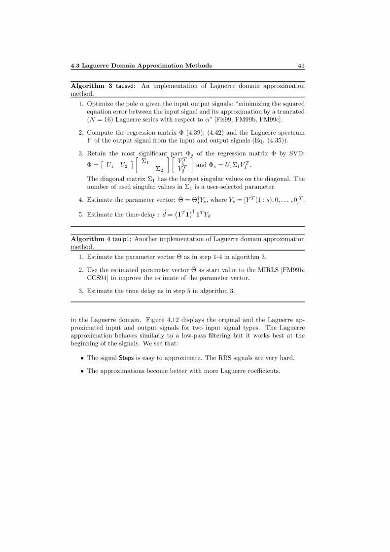
4.3 Laguerre Domain Approximation Methods 41
Algorithm 3 tausvd: An implementation of Laguerre domain approximationmethod.
1. Optimize the pole α given the input output signals: “minimizing the squaredequation error between the input signal and its approximation by a truncated(N = 16) Laguerre series with respect to α” [Fis99, FM99b, FM99c].
2. Compute the regression matrix Φ (4.39), (4.42) and the Laguerre spectrumY of the output signal from the input and output signals (Eq. (4.35)).
3. Retain the most significant part Φs of the regression matrix Φ by SVD:
Φ =[U1 U2
] [ Σ1
Σ2
] [V T1V T2
]and Φs = U1Σ1V
T1 .
The diagonal matrix Σ1 has the largest singular values on the diagonal. Thenumber of used singular values in Σ1 is a user-selected parameter.
4. Estimate the parameter vector: Θ = Θ†sYs, where Ys = [Y T (1 : s), 0, . . . , 0]T .
5. Estimate the time-delay : d =(1T1
)†1TYd
Algorithm 4 taulp1: Another implementation of Laguerre domain approximationmethod.
1. Estimate the parameter vector Θ as in step 1-4 in algorithm 3.
2. Use the estimated parameter vector Θ as start value to the MIRLS [FM99b,CCS94] to improve the estimate of the parameter vector.
3. Estimate the time delay as in step 5 in algorithm 3.
in the Laguerre domain. Figure 4.12 displays the original and the Laguerre ap-proximated input and output signals for two input signal types. The Laguerreapproximation behaves similarly to a low-pass filtering but it works best at thebeginning of the signals. We see that:
• The signal Steps is easy to approximate. The RBS signals are very hard.
• The approximations become better with more Laguerre coefficients.
42 Chapter 4 Time-Delay Approximation Methods
Figure 4.12 Original and Laguerre approximated input and output signal for RBS0-100% (left) and Steps (right) with N + 1 = 51 (above) and N + 1 = 150 (below).Laguerre pole α = 0.8, G2, SNR=100. The signals and the system are defined inSection 7.3. N + 1 is the number of used Laguerre functions. (t222b1-t222b2)
0 50 100 150 200 250 300 350 400 450 500−2
−1
0
1
2t222b1 Input signal
0 50 100 150 200 250 300 350 400 450 500−2
−1
0
1
2t222b1 Output signal
PSfrag replacements
tu(t)y(t)s(t)
gts(t)
TdTd
δ(t− Td)g(t)gr(t)g(t)
0 50 100 150 200 250 300 350 400 450 500−2
−1
0
1
2t222b1 Input signal
0 50 100 150 200 250 300 350 400 450 500−2
−1
0
1
2t222b1 Output signal
PSfrag replacements
tu(t)y(t)s(t)
gts(t)
TdTd
δ(t− Td)g(t)gr(t)g(t)
0 50 100 150 200 250 300 350 400 450 500−2
−1
0
1
2t222b2 Input signal
0 50 100 150 200 250 300 350 400 450 500−2
−1
0
1
2t222b2 Output signal
PSfrag replacements
tu(t)y(t)s(t)
gts(t)
TdTd
δ(t− Td)g(t)gr(t)g(t)
0 50 100 150 200 250 300 350 400 450 500−2
−1
0
1
2t222b2 Input signal
0 50 100 150 200 250 300 350 400 450 500−2
−1
0
1
2t222b2 Output signal
PSfrag replacements
tu(t)y(t)s(t)
gts(t)
TdTd
δ(t− Td)g(t)gr(t)g(t)
5Explicit Time-Delay Parameter
Methods
In explicit time-delay parameter methods, the time-delay is an explicit parameter tobe estimated in the model. In Section 5.1 the time-delay is a continuous parameterin a continuous-time model, while in Section 5.2 a discrete parameter in a discrete-time model. Section 5.3 describes some sampling methods.
5.1 Continuous-Time One-Step Explicit Methods
In continuous-time one-step explicit methods, the time-delay is modeled and es-timated as a continuous parameter in a continuous-time model. The time-delayis thus not restricted to be a multiple of the sampling interval. See for exam-ple [NL91, Lju02].
5.1.1 The time-delay estimation methods
Here we will describe a group of methods consists of estimating the time-delay as acontinuous parameter with the prediction error method (Section 4.1.5 and[Lju99])in some simple model structures [Lju02] which are often used in process industry.We sometimes call this type of methods idproc methods. The process models are:
idproc1. A first order system with time-delay.
idproc2. A second order system with real poles and time-delay.
idproc3. A second order system with complex poles and time-delay.
43
44 Chapter 5 Explicit Time-Delay Parameter Methods
idproc4. A third order system with real poles and time-delay.
idproc5. A third order system with two complex poles, one real pole and time-delay.
In the prediction error method (PEM) [Lju99]:
θN = arg minθVN (θ) = arg min
θ
1
N
N∑
t=1
1
2ε2(t, θ), (5.1)
where ε(t|θ) = y(t) − y(t|θ) is the prediction error of the model. See also Sec-tion 4.1.5.
Since the loss function VN (θ) in Equation (5.1) has several minima [FMS96,NL91], the initialization of the optimization problem (5.1) must be done care-fully [Lju02]. See [Lju03, BL03] for the implementation used in the simulationsof this thesis. An alternative to accurately initialize the time-delay could be toperform a low-pass filtering. See Section 5.1.3.
The article [NL91] contains formulas for zoh sampling of a system with time-delay in state space form including a noise model. It also contains Matlab codefor how to implement a PEM algorithm.
5.1.2 Local minima of a first order system
We will here study the phenomenon that the loss function VN (θ) in Equation (5.1)has several minima more closely.
Assume, both the true system and the model is of the same structure: a firstorder system with time-delay:
G(s) =K
s+ βe−sL. (5.2)
The system sampled with the sampling interval Ts using zero-order-hold (zoh)
sampling [AW84] becomes
y(k) =b1q−1 + b2q
−2
1 + a1q−1u(k) = G(q)u(k) (5.3)
with
b1 = Ke−β(Ts−L)
β(e−β(Ts−L) − 1) (5.4)
b2 = Ke−β(Ts−L)
β(1− e−βL) (5.5)
a1 = −e−βTs . (5.6)
We will denote the true system with Go(s) (in continuous-time) and Go(q) (thesampled discrete-time version of Go(s)) and its parameters with b10, b20 and a10.
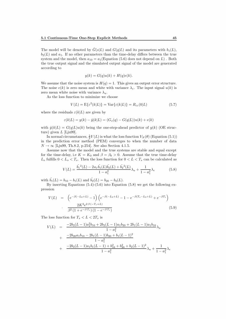
5.1 Continuous-Time One-Step Explicit Methods 45
The model will be denoted by G(s|L) and G(q|L) and its parameters with b1(L),b2(L) and a1. If no other parameters than the time-delay differs between the truesystem and the model, then a10 = a1(Equation (5.6) does not depend on L) . Boththe true output signal and the simulated output signal of the model are generatedaccording to
y(k) = G(q)u(k) +H(q)e(k).
We assume that the noise system is H(q) = 1. This gives an output error structure.The noise e(k) is zero mean and white with variance λe. The input signal u(k) iszero mean white noise with variance λu.
As the loss function to minimize we choose
V (L) = E{ε2(k|L)} = Var{ε(k|L)} = Rεε(0|L) (5.7)
where the residuals ε(k|L) are given by
ε(k|L) = y(k)− y(k|L) = (Go(q)−G(q|L))u(k) + e(k)
with y(k|L) = G(q|L)u(k) being the one-step-ahead predictor of y(k) (OE struc-ture) given L [Lju99].
In normal circumstances, 12V (L) is what the loss function VN (θ) (Equation (5.1))
in the prediction error method (PEM) converges to when the number of dataN →∞ [Lju99, Th.8.2, p.254]. See also Section 4.1.5.
Assume now that the model and the true systems are stable and equal exceptfor the time-delay, i.e K = K0 and β = β0 > 0. Assume that the true time-delayLo fulfills 0 < Lo < Ts. Then the loss function for 0 < L < Ts can be calculated as
V (L) =b1
2(L)− 2a1 b1(L)b2(L) + b22(L)
1− a21
λu +1
1− a21
λe (5.8)
with b1(L) = b10 − b1(L) and b2(L) = b20 − b2(L).By inserting Equations (5.4)-(5.6) into Equation (5.8) we get the following ex-
pression
V (L) =(e−β(−L0+L) − 1
)(e−β(−L0+L) − 1− e−β(Ts−L0+L) + e−βTs
)
· 2K2e2β (−Ts+L)
β2 (1 + e−β Ts) (1− e−β Ts) (5.9)
The loss function for Ts < L < 2Ts is
V (L) =−2b2(L− 1)a2
1b10 + 2b2(L− 1)a1b20 + 2b1(L− 1)a1b10
1− a21
λu
+−2b20a1b10 − 2b1(L− 1)b20 + b1(L− 1)2
1− a21
+−2b2(L− 1)a1b1(L− 1) + b210 + b220 + b2(L− 1)2
1− a21
λu +1
1− a21
λe
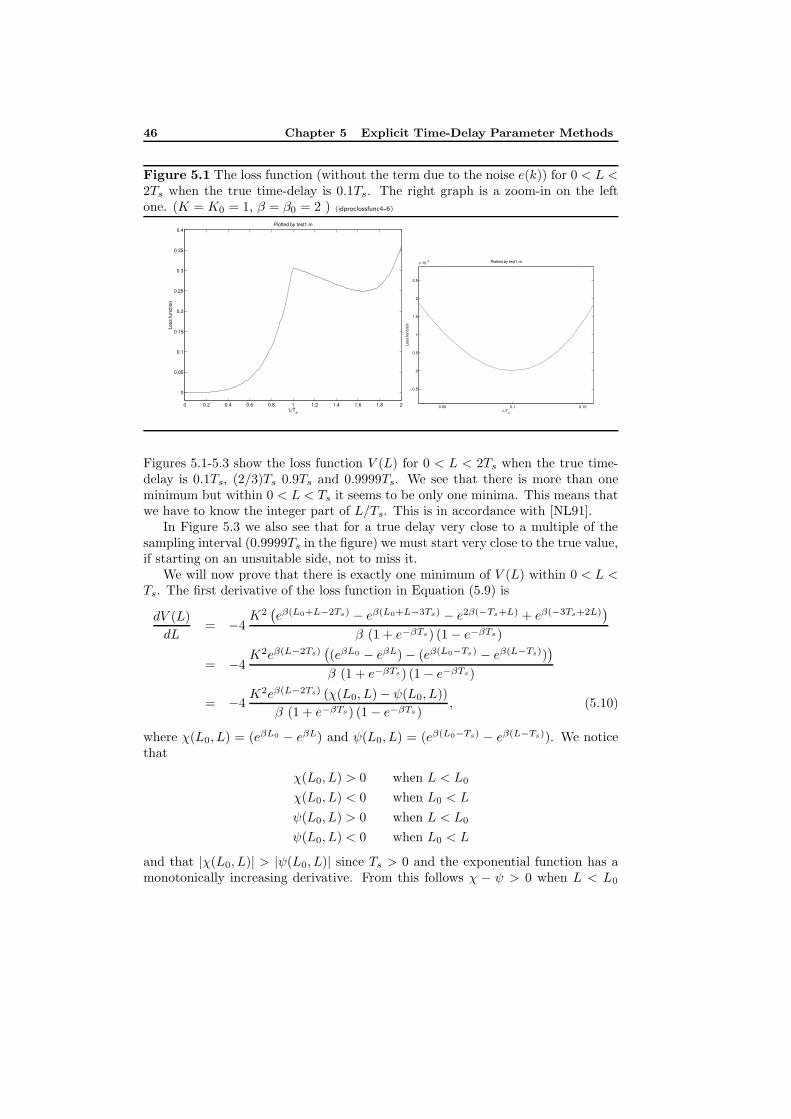
46 Chapter 5 Explicit Time-Delay Parameter Methods
Figure 5.1 The loss function (without the term due to the noise e(k)) for 0 < L <2Ts when the true time-delay is 0.1Ts. The right graph is a zoom-in on the leftone. (K = K0 = 1, β = β0 = 2 ) (idproclossfunc4-6)
0 0.2 0.4 0.6 0.8 1 1.2 1.4 1.6 1.8 2
0
0.05
0.1
0.15
0.2
0.25
0.3
0.35
0.4Plotted by test1.m
Loss
func
tion
L/Ts
PSfrag replacements
tu(t)y(t)s(t)
gts(t)
TdTd
δ(t− Td)g(t)gr(t)g(t)
0.05 0.1 0.15
−0.5
0
0.5
1
1.5
2
2.5
x 10−4 Plotted by test1.m
Loss
func
tion
L/Ts
PSfrag replacements
tu(t)y(t)s(t)
gts(t)
TdTd
δ(t− Td)g(t)gr(t)g(t)
Figures 5.1-5.3 show the loss function V (L) for 0 < L < 2Ts when the true time-delay is 0.1Ts, (2/3)Ts 0.9Ts and 0.9999Ts. We see that there is more than oneminimum but within 0 < L < Ts it seems to be only one minima. This means thatwe have to know the integer part of L/Ts. This is in accordance with [NL91].
In Figure 5.3 we also see that for a true delay very close to a multiple of thesampling interval (0.9999Ts in the figure) we must start very close to the true value,if starting on an unsuitable side, not to miss it.
We will now prove that there is exactly one minimum of V (L) within 0 < L <Ts. The first derivative of the loss function in Equation (5.9) is
dV (L)
dL= −4
K2(eβ(L0+L−2Ts) − eβ(L0+L−3Ts) − e2β(−Ts+L) + eβ(−3Ts+2L)
)
β (1 + e−βTs) (1− e−βTs)
= −4K2eβ(L−2Ts)
((eβL0 − eβL)− (eβ(L0−Ts) − eβ(L−Ts))
)
β (1 + e−βTs) (1− e−βTs)
= −4K2eβ(L−2Ts) (χ(L0, L)− ψ(L0, L))
β (1 + e−βTs) (1− e−βTs) , (5.10)
where χ(L0, L) = (eβL0 − eβL) and ψ(L0, L) = (eβ(L0−Ts) − eβ(L−Ts)). We noticethat
χ(L0, L) > 0 when L < L0
χ(L0, L) < 0 when L0 < L
ψ(L0, L) > 0 when L < L0
ψ(L0, L) < 0 when L0 < L
and that |χ(L0, L)| > |ψ(L0, L)| since Ts > 0 and the exponential function has amonotonically increasing derivative. From this follows χ − ψ > 0 when L < L0
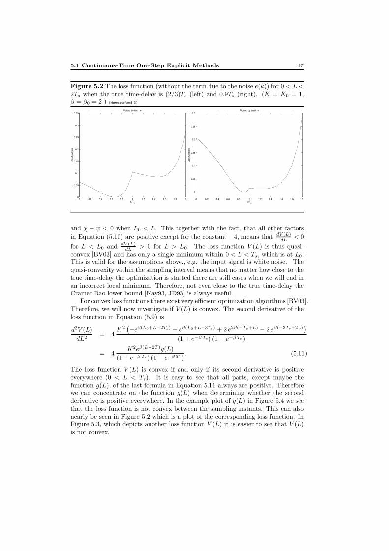
5.1 Continuous-Time One-Step Explicit Methods 47
Figure 5.2 The loss function (without the term due to the noise e(k)) for 0 < L <2Ts when the true time-delay is (2/3)Ts (left) and 0.9Ts (right). (K = K0 = 1,β = β0 = 2 ) (idproclossfunc1-3)
0 0.2 0.4 0.6 0.8 1 1.2 1.4 1.6 1.8 20
0.05
0.1
0.15
0.2
0.25
0.3
0.35Plotted by test1.m
Loss
func
tion
L/Ts
PSfrag replacements
tu(t)y(t)s(t)
gts(t)
TdTd
δ(t− Td)g(t)gr(t)g(t)
0 0.2 0.4 0.6 0.8 1 1.2 1.4 1.6 1.8 2
0
0.05
0.1
0.15
0.2
0.25
0.3Plotted by test1.m
Loss
func
tion
L/Ts
PSfrag replacements
tu(t)y(t)s(t)
gts(t)
TdTd
δ(t− Td)g(t)gr(t)g(t)
and χ − ψ < 0 when L0 < L. This together with the fact, that all other factors
in Equation (5.10) are positive except for the constant −4, means that dV (L)dL < 0
for L < L0 and dV (L)dL > 0 for L > L0. The loss function V (L) is thus quasi-
convex [BV03] and has only a single minimum within 0 < L < Ts, which is at L0.This is valid for the assumptions above., e.g. the input signal is white noise. Thequasi-convexity within the sampling interval means that no matter how close to thetrue time-delay the optimization is started there are still cases when we will end inan incorrect local minimum. Therefore, not even close to the true time-delay theCramer Rao lower bound [Kay93, JD93] is always useful.
For convex loss functions there exist very efficient optimization algorithms [BV03].Therefore, we will now investigate if V (L) is convex. The second derivative of theloss function in Equation (5.9) is
d2V (L)
dL2= 4
K2(−eβ(L0+L−2Ts) + eβ(L0+L−3Ts) + 2 e2β(−Ts+L) − 2 eβ(−3Ts+2L)
)
(1 + e−β Ts) (1− e−β Ts)
= 4K2eβ(L−2T )g(L)
(1 + e−β Ts) (1− e−β Ts) . (5.11)
The loss function V (L) is convex if and only if its second derivative is positiveeverywhere (0 < L < Ts). It is easy to see that all parts, except maybe thefunction g(L), of the last formula in Equation 5.11 always are positive. Thereforewe can concentrate on the function g(L) when determining whether the secondderivative is positive everywhere. In the example plot of g(L) in Figure 5.4 we seethat the loss function is not convex between the sampling instants. This can alsonearly be seen in Figure 5.2 which is a plot of the corresponding loss function. InFigure 5.3, which depicts another loss function V (L) it is easier to see that V (L)is not convex.
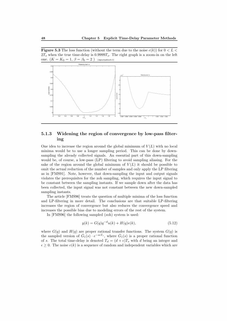
48 Chapter 5 Explicit Time-Delay Parameter Methods
Figure 5.3 The loss function (without the term due to the noise e(k)) for 0 < L <2Ts when the true time-delay is 0.9999Ts. The right graph is a zoom-in on the leftone. (K = K0 = 1, β = β0 = 2 ) (idproclossfunc5-2)
0 0.2 0.4 0.6 0.8 1 1.2 1.4 1.6 1.8 2
0
0.05
0.1
0.15
0.2
0.25
0.3
0.35
0.4Plotted by test1.m
Loss
func
tion
L/Ts
PSfrag replacements
tu(t)y(t)s(t)
gts(t)
TdTd
δ(t− Td)g(t)gr(t)g(t)
0.9997 0.9998 0.9998 0.9999 0.9999 1 1 1 1.0001 1.0002 1.0002
−0.5
0
0.5
1
1.5
2
2.5
3
x 10−8 Plotted by test1.m
Loss
func
tion
L/Ts
PSfrag replacements
tu(t)y(t)s(t)
gts(t)
TdTd
δ(t− Td)g(t)gr(t)g(t)
5.1.3 Widening the region of convergence by low-pass filter-ing
One idea to increase the region around the global minimum of V (L) with no localminima would be to use a longer sampling period. This can be done by down-sampling the already collected signals. An essential part of this down-samplingwould be, of course, a low-pass (LP) filtering to avoid sampling aliasing. For thesake of the region around the global minimum of V (L) it should be possible toomit the actual reduction of the number of samples and only apply the LP filteringas in [FMS91]. Note, however, that down-sampling the input and output signalsviolates the prerequisites for the zoh sampling, which requires the input signal tobe constant between the sampling instants. If we sample down after the data hasbeen collected, the input signal was not constant between the new down-sampledsampling instants.
The article [FMS96] treats the question of multiple minima of the loss functionand LP-filtering in more detail. The conclusions are that suitable LP-filteringincreases the region of convergence but also reduces the convergence speed andincreases the possible bias due to modeling errors of the rest of the system.
In [FMS96] the following sampled (zoh) system is used:
y(k) = G(q)q−du(k) +H(q)e(k), (5.12)
where G(q) and H(q) are proper rational transfer functions. The system G(q) isthe sampled version of G1(s) · e−sεTs , where G1(s) is a proper rational functionof s. The total time-delay is denoted Td = (d + ε)Ts with d being an integer andε ≥ 0. The noise e(k) is a sequence of random and independent variables which are
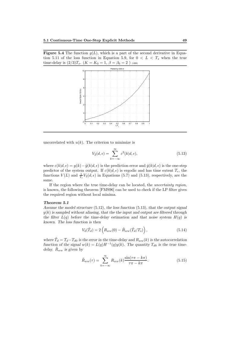
5.1 Continuous-Time One-Step Explicit Methods 49
Figure 5.4 The function g(L), which is a part of the second derivative in Equa-tion 5.11 of the loss function in Equation 5.9, for 0 < L < Ts when the truetime-delay is (2/3)Ts. (K = K0 = 1, β = β0 = 2 ) (t300)
0 0.1 0.2 0.3 0.4 0.5 0.6 0.7 0.8 0.9 1−2
0
2
4
6
8
10
L/Ts
\frac
{d^2
}{dL
^2}V
(L)
Plotted by t300.m
PSfrag replacements
tu(t)y(t)s(t)
gts(t)
TdTd
δ(t− Td)g(t)gr(t)g(t)
uncorrelated with u(k). The criterion to minimize is
V2(d, ε) =∞∑
k=−∞ε2(k|d, ε), (5.13)
where ε(k|d, ε) = y(k)− y(k|d, ε) is the prediction error and y(k|d, ε) is the one-steppredictor of the system output. If ε(k|d, ε) is ergodic and has time extent Tε, thefunctions V (L) and 1
TεV2(d, ε) in Equations (5.7) and (5.13), respectively, are the
same.If the region where the true time-delay can be located, the uncertainty region,
is known, the following theorem [FMS96] can be used to check if the LP filter givesthe required region without local minima.
Theorem 5.1Assume the model structure (5.12), the loss function (5.13), that the output signaly(k) is sampled without aliasing, that the the input and output are filtered throughthe filter L(q) before the time-delay estimation and that noise system H(q) isknown. The loss function is then
V2(Td) = 2(Rww(0)− Rww(Td/Ts)
), (5.14)
where Td = Td−Td0 is the error in the time-delay and Rww(k) is the autocorrelationfunction of the signal w(k) = L(q)H−1(q)y(k). The quantity Td0 is the true time-delay. Rww is given by
Rww(τ) =
∞∑
k=−∞Rww(k)
sin(τπ − kπ)
τπ − kπ . (5.15)
50 Chapter 5 Explicit Time-Delay Parameter Methods
Note that in Equation (5.14), only the difference Td between the estimated andtrue time-delay matters and that Td is not restricted to multiples of the samplinginterval but can take any value.
In the special case when L(eiωTs)H−1(eiωTs)G(iω) is an ideal LP filter withcutoff frequency ωb and the input signal is white noise, [FMS96] shows that thecutoff frequency of the LP filter should be selected as
ωb .4.49
∆Td,
where ∆Td is the largest time-delay uncertainty. The rational part of the sampledsystem G(q) is assumed known.
In the case of aliasing by the sampling and/or poor filtering, [FMS96] say thatthere may be many local minima, each belonging to a sampling interval.
Another way to accomplish the “widening of the sampling interval” withoutdown-sampling could be to let the input signal be of low-pass type. This is similarbut not equivalent to LP-filtering the input-output data (see [Lju99, p. 266-267,466-468]).
5.2 Discrete-Time One-Step Explicit Methods
In discrete-time one-step explicit methods, the time-delay is modeled and estimatedas a discrete parameter in a discrete-time model. Estimating several models, e.g.ARX models, with a complete set of time-delays and choosing the best is of thissubclass ([Swa99, IHD00]). An exhaustive search is thus performed in the time-delay dimension. This subclass of methods is here also called arxstruc type methods.All methods described in this section are of this subclass. In Section 5.2.1 ARXmodels are utilized, in Section 5.2.2 OE models and in Section 5.2.3 prefilteredARX models.
5.2.1 Arxstruc
In the method arxstruc several ARX models [Lju99]
A(q)y(t) = B(q)u(t− nk) + e(t)
are estimated with PEM (Prediction Error Method) ([Lju99] and Section 4.1.5)for different time-delays nk. PEM is here equal to Least Squares Estimation(LSE) [Lju99]. The delay whose model has the lowest loss function is chosen.The estimation is quick since the ARX model can be written as a linear regressionand can be estimated by solving a linear equation system [Lju99]. See Algorithm 5for Matlab code using the Matlab System Identification Toolbox.
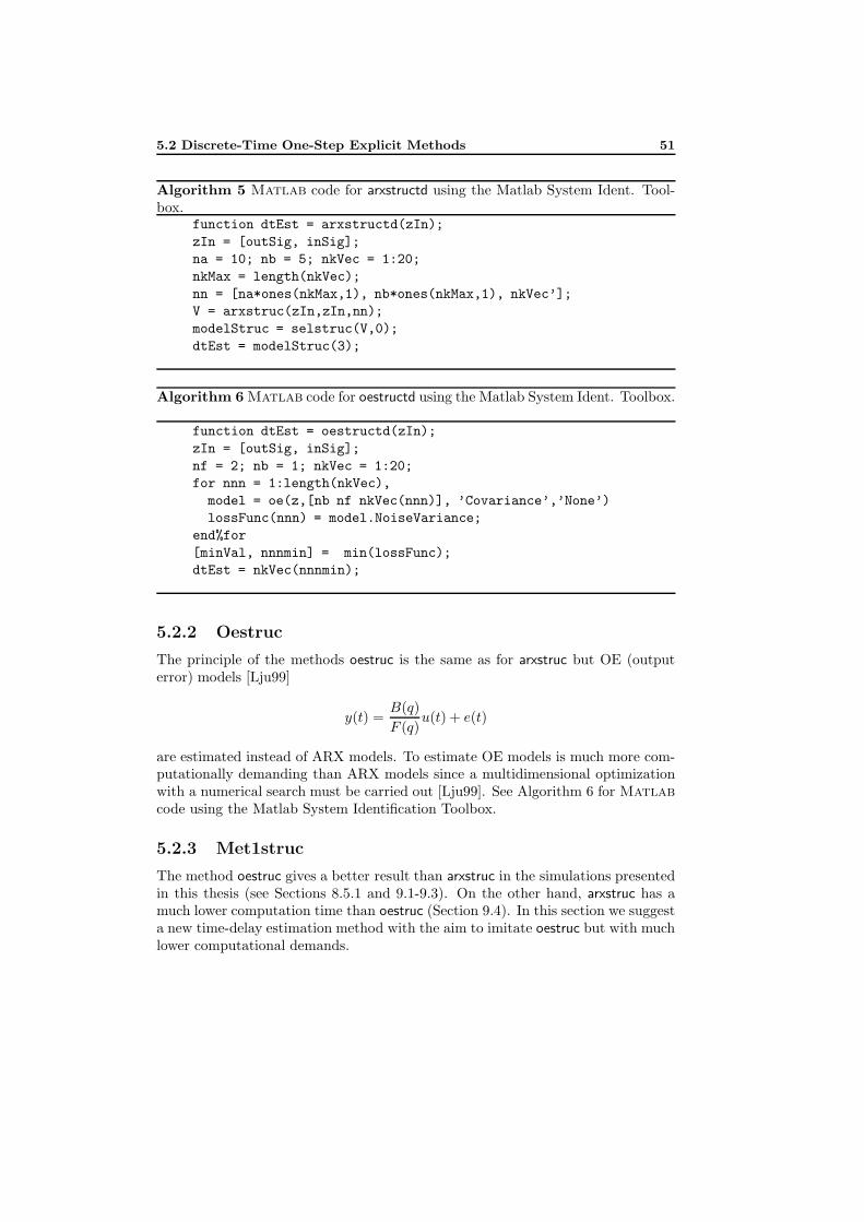
5.2 Discrete-Time One-Step Explicit Methods 51
Algorithm 5 Matlab code for arxstructd using the Matlab System Ident. Tool-box.
function dtEst = arxstructd(zIn);
zIn = [outSig, inSig];
na = 10; nb = 5; nkVec = 1:20;
nkMax = length(nkVec);
nn = [na*ones(nkMax,1), nb*ones(nkMax,1), nkVec’];
V = arxstruc(zIn,zIn,nn);
modelStruc = selstruc(V,0);
dtEst = modelStruc(3);
Algorithm 6 Matlab code for oestructd using the Matlab System Ident. Toolbox.
function dtEst = oestructd(zIn);
zIn = [outSig, inSig];
nf = 2; nb = 1; nkVec = 1:20;
for nnn = 1:length(nkVec),
model = oe(z,[nb nf nkVec(nnn)], ’Covariance’,’None’)
lossFunc(nnn) = model.NoiseVariance;
end%for
[minVal, nnnmin] = min(lossFunc);
dtEst = nkVec(nnnmin);
5.2.2 Oestruc
The principle of the methods oestruc is the same as for arxstruc but OE (outputerror) models [Lju99]
y(t) =B(q)
F (q)u(t) + e(t)
are estimated instead of ARX models. To estimate OE models is much more com-putationally demanding than ARX models since a multidimensional optimizationwith a numerical search must be carried out [Lju99]. See Algorithm 6 for Matlabcode using the Matlab System Identification Toolbox.
5.2.3 Met1struc
The method oestruc gives a better result than arxstruc in the simulations presentedin this thesis (see Sections 8.5.1 and 9.1-9.3). On the other hand, arxstruc has amuch lower computation time than oestruc (Section 9.4). In this section we suggesta new time-delay estimation method with the aim to imitate oestruc but with muchlower computational demands.
52 Chapter 5 Explicit Time-Delay Parameter Methods
Assume the true system is given by
y = G0u+H0e ,
where G0 and H0 are rational functions in the delay operator q−1. The noise e iswhite. The model structure used to estimate the true system is
y = Gu+He ,
where G and H also are rational functions.The reason for the difference between OE and ARX model structures can be
two-fold:
1. If the model structure G cannot exactly describe the true system G0, theestimated model G will have a bias, even if the number of data N →∞. TheOE and ARX model structures will behave differently in open loop [Lju99,Ex. 8.5, p. 268-269]:
• The ARX model structure will give models with a good fit to the truesystem at high frequencies.
• The OE model structure will give models with a good fit to the truesystem at low frequencies if the input is of low frequency character.
2. If the model structure G can exactly describe the true system G0, again theOE and ARX model structures behave differently in open loop:
• The ARX model structure will give models G with a bias if the noisemodel structure 1/A cannot describe the true noise systemH0. See [Lju99,eq. 8.63,8.69, p. 267].
• The OE model structure will give estimates without bias. The bias ofthe OE model structure is thus not dependent on the noise model. See[Lju99, Eq. 8.71, p. 266].
We propose the time-delay estimation method in Algorithm 7. The motivation forthis method is the following. Assume the true system is given by
y = G0u+H0e =B0
F0u+
C0
D0e ,
where G0 and H0 are rational functions and B0, F0, C0 and D0 are polynomials inthe delay operator q−1. The noise e is white.
Estimate a first model
y =B1
F1u+
C1
D1e (5.16)
where F1, B1, C1 and D1 are polynomials in q−1, i.e. a Box-Jenkins model [Lju99].
5.2 Discrete-Time One-Step Explicit Methods 53
Algorithm 7 Proposed time-delay estimation method (prefiltered arxstruc).
1. Estimate an ARMAX model A1(q)y(k) = B1(q)u(k) + C1(q)e(k).
2. Prefilter u and y through 1/C1(q) .
3. Arxstruc gives an estimate of nk.
The model C1/D1 will be an approximation of H0 = C0/D0. Then, filter theoutput signal y through D1/C1 giving yF :
yF =D1
C1y =
D1
C1
(B0
F0u+H0e
)=B0
F0
D1
C1u+H0
D1
C1e =
B0
F0uF +H0
D1
C1e ,
(5.17)
where uF = uD1/C1 is the input signal u filtered through D1/C1. Now, if thepolynomials F1, B1, C1 and D1 in the model structure 5.16 have high enoughorders so that that they can exactly describe the true system and the input-outputdata is informative enough, then F1, B1, C1 and D1 will converge to the true valuesF0, B0, C0 and D0 as the number of data N → ∞ [Lju99, p. 273]. When thishappens, D1/C1 = 1/H0 and Equation 5.17 simplifies to
F0yF = B0uF + e , (5.18)
where e as before is white noise. This true system is obviously an ARX system.This means that if we estimate an ARX model AyF = BuF + e, there will be nobias due to an incorrect noise model. If an ARX model has high enough orders, wecan get a model for the system G without bias (as in the case with an OE modelof high enough orders).
Let us now assume that the true system instead has OE structure:
y = G0u+H0e =B0
F0u+ e ⇒ F0y = B0u+ F0e. (5.19)
As this at the same time has ARMAX structure [Lju99] we estimate a first model
A1y = B1u+ C1e , (5.20)
where A1, B1 and C1 are polynomials in q−1. A1 and C1 will be approximations ofF0. If we filter the input and output signal through 1/C1 we will get the followingtrue system
F0yF = B0uF + e , (5.21)
which is also of ARX structure and can be approximated by an ARX model of highenough model order without bias.
54 Chapter 5 Explicit Time-Delay Parameter Methods
Algorithm 8 met1struc, the prefiltered arxstruc.
1. Estimating a state space model by state space method.
2. Converting to A1(q)y(k) = B1(q)u(k) + C1(q)e(k) .
3. Prefiltering u and y through 1/C1(q) .
4. Arxstruc gives an estimate of nk.
Algorithm 9 Matlab code for met1struc using the Matlab System IdentificationToolbox. The function arxstructd is described in Section 5.2.1.
function dtEst = met1structd(inSig, outSig, Ts)
order = 10;
modelSs = n4sid(iddata(outSig, inSig, Ts),...
order,’cov’,’none’);
[A,B,C,D,F] = polydata(idpoly(modelSs));
BFilt = 1;
AFilt = C;
uFilt = filter(BFilt,AFilt,inSig);
yFilt = filter(BFilt,AFilt,outSig);
zIn = [yFilt, uFilt];
na = 10; nb = 1; nkVec = 1:20;
dtEst = arxstructd(zIn,nkVec,na,nb);
Since the systems employed in most simulations in this thesis (Section 7.3) haveOE structure (Equation (5.19)), we will filter the input and output signals through1/C1 where C1 is from Equation (5.20).
In Algorithm 7 the first step is to estimate an ARMAX model. Unfortunately,the standard way to estimate a model of this structure also requires a numericalsearch as with the OE model which we tried to avoid. Another way is to firstestimate a state space model and then convert it to an ARMAX model. Thisconversion will be possible if the order of the state space model and the ordersof the polynomials A1, B1 and C1 are high enough to describe the true system.The state space model can be quickly estimated by a subspace method [Lju99].See Algorithm 8 for the resulting method, which we call met1struc. Matlab codefor met1struc is given in Algorithm 9. The order of the state space model is 10.This will hopefully be enough for most systems. The orders of A1, B1 and C1 willdepend on the order of the state space model.
5.3 Sampling Methods 55
5.3 Sampling Methods
Sampling methods utilize the sampling process to estimate the time-delay. Forexample, zero-order-hold (zoh) sampling of a system with subsample time-delayscreates an extra zero [FMS91] as we will see soon.
5.3.1 Principles
We start with an example of sampling a simple system without time-delay. Weconsider the following continuous-time system:
G(s) =K
s+ β. (5.22)
The system sampled with the sampling interval Ts using zero-order-hold (zoh) sam-
pling, i.e. the input signal is constant between the sampling instants, (see[AW84,GL97]) becomes :
G(q) = µ(1− p)(q − p) , (5.23)
with
µ = K/β (5.24)
and
p = e−βTs . (5.25)
The letter q is the discrete-time-delay operator, i.e. q−1 is a delay of one sample.When zoh sampling of a continuous-time system with a time-delay which is a
fraction of a sampling interval is performed, a zero in the discrete-time system willarise due to the time-delay [AW84, p. 40]. We now will see what happens at thesampling when a time-delay is added to the previous example.
Assume that we have the same continuous-time system as in Equation (5.22)but now with a time-delay 0 < L < Ts:
G(s) =K
s+ βe−sL = G1(s) · e−sL. (5.26)
The system sampled with the sampling interval Ts using zoh sampling becomes (cf.Section 5.1.2)
G(q) =b1q−1 + b2q
−2
1 + a1q−1= µ
(1− p)(q − p) ·
((1− α)q + α)
q. (5.27)
The quantities a1, b1 and b2 are given by Equations (5.4)-(5.6) and µ and p byEquations (5.24) and (5.25). The quantity α is given by
α =eβL − 1
1− p p. (5.28)
56 Chapter 5 Explicit Time-Delay Parameter Methods
We see from Equations (5.23) and (5.27) that the result of the time-delay after thesampling is a pole in zero and an additional zero:
z0 = − α
(1− α). (5.29)
If the time-delay is longer, d ·Ts < dTs+L < (d+1) ·Ts, (L is thus the fractional
part of the time-delay), the sampled system will be [AW84, FMS91]
G(q) =b1q−1 + b2q
−2
1 + a1q−1q−d = µ
(1− p)(q − p) ·
((1− α)q + α)
qq−d. (5.30)
The only difference to Equation (5.27) is the extra factor q−d because of the integerpart d ·Ts of the time-delay. The zero due to the fractional part L of the time-delayis the same as before (Equation (5.29)).
The sampled version of a proper rational continuous-time system with m zerosand n poles has generically n − 1 discrete-time zeros, some of which may go toinfinity or be canceled by poles [ASH84]. The sampled version of a continuous-time system can have zeros due to three reasons:
1. Zeros of the continuous-time system [ASH84].
2. Zeros created by the sampling process for a continuous-time system withoutfractional time-delay. Some of these zeros may be “unstable”, i.e. be outsidethe unit circle. Whether they are outside the unit circle, depends on n −mand the sampling interval Ts. If n −m < 2 or the sampling interval is longenough, these zeros are always inside the unit circle. See [ASH84].
3. Zeros created by the sampling process for a continuous-time system withfractional time-delay [FMS91, AW84].
In [FMS91] it is said that “sampling zeros”, of type 2 above, does not significantlyaffect the result of the estimation. This conclusion is based upon a simple example.
5.3.2 Recursive TIDEA
In [FMS91] the fact that α→ L/Ts = ε when Ts → 0 is utilized. We call ε the nor-malized fractional time-delay. Using this we see that the zero z0 (Equation (5.29))of the system in Equation (5.27) can be written
z0 = − α
(1− α)≈ − ε
1− ε
for small sampling intervals. We can solve for ε in this expression:
ε =1
1− z0.
5.3 Sampling Methods 57
In [FMS91] an extended model structure, compared to Equation (5.30) is employed:
G(q) = q−(d+1) b2q2 + b1q + b0AR(q)
, (5.31)
where AR(q) is a polynomial in q with a high enough degree.This model structure (due to the numerator b2q
2 + b1q + b0) can handle nor-malized fractional time-delays −1 < ε < 1, not only 0 < ε < 1 as in Section 5.3.1,without changing the normalized integer part d of the time-delay.
Also, higher order true systems than a first order system as in Section 5.3.1can be modeled thanks to the denominator AR(q). Requirements for this is thatthe true continuous-time system does not have any zero on the imaginary axisand that the sampling interval is small enough. If the true time-delay is wanted,the polynomial AR(q) should have a high enough degree for 1/AR(q) to accuratelydescribe the rational part G1(s) of the time-delay system. On the other hand, if therole of the time-delay is to adjust the phase of the model in an important frequencyrange, AR(q) can have a low degree. Compare with Section 1.1.
In [FMS91] time-delay estimation method, called TIDEA (TIme Delay Estima-tion Algorithm), based on the above, is presented. The model (5.31) is estimatedrecursively. TIDEA also contains a special mechanism for adjusting the normalizedinteger part d of the time-delay. See [FMS91] for details. According to [FMS91],the global convergence of TIDEA is still not proved. We did not succeed to imple-ment the method without it diverging. Therefore we have no simulation results forthis method.
5.3.3 Exact time-delay from the sampling process
The zero-order-hold sampling of the model structure (5.26) is described in Sec-tion 5.3.1. Assume that all model parameters except for the time-delay are known.From Equations (5.25), (5.28) and (5.29) it is easy to solve for the fractional time-delay L:
L =1
βln
(1− eβTsz0
1− z0
)(5.32)
Note, that this expression does not require that Ts → 0 as in TIDEA (Section 5.3.2).The integer part of the time-delay must be estimated in some other way, e.g. as inTIDEA or with oestruc (Section 5.2.2).
In [ASH84] the system
G(s) =1
sesL
is zoh sampled, giving
G(p) =(Ts − L)q + L
q(q − 1)
58 Chapter 5 Explicit Time-Delay Parameter Methods
with the zero
z0 = − L
Ts − L. (5.33)
By solving for the fractional time-delay L in Equation (5.33), we get
L =z0Tsz0 − 1
.
6Area, Moment and Higher-Order
Statistics Methods
Area and moment methods (Sections 6.1-6.3) utilize relations between the time-delay and certain areas above or below the step response s(t) and certain momentsof the impulse response h(t) (integrals of the type
∫tnh(t)dt). Higher-order statis-
tics (HOS) methods (Section 6.4) use HOS to discriminate between symmetricprobability distribution, e.g. Gaussian, and non-symmetric. They are are suitablewhen desired and undesired signals differ in this aspect.
6.1 Area Methods
In [AH95] some methods for identifying simple process models of the kind
G(s) =K
1 + sTesL (6.1)
and
G(s) =K
(1− sT )2esL (6.2)
are described. Part of this identification is the estimation of the time-delay L,which is what we are interested in here.
Area methods [AH95] use area calculations of a step response s(t). First theaverage residence time Tar is calculated as
Tar =A0
K,
59
60 Chapter 6 Area, Moment and Higher-Order Statistics Methods
where K = s(∞) is the static gain and the area A0 is calculated from
A0 =
∫ ∞
0
(s(∞) − s(t))dt. (6.3)
The average residence time is a rough measure of the time for the step response tofinish. Then we calculate
A1 =
∫ Tar
0
s(t)dt. (6.4)
For the first order model (6.1) the time constant is then given by
T =e1A1
K. (6.5)
The time-delay is
L = Tar − T.
For the second order model (6.2) the time constant is given by
T =e2A1
4K(6.6)
and the time-delay is
L = Tar − 2T.
See [AH95] for the derivation of these area methods. In [AH95] they use a real stepresponse from a step response experiment when identifying the system with thesemethods. In this thesis we will use an arbitrary input signal and first estimate thestep response before applying the methods.
6.2 Moment Methods
In moment methods [AH95] we interpret the normalized impulse response
f(t) =h(t)∫∞
0h(t)dt
of the system as a probability density function. The quantity h(t) is the impulseresponse. Then we can call the quantities
mn =
∫ ∞
0
tnf(t)dt (6.7)
the moment of order n. For the first order model (6.1) the static gain is given by
K =
∫ ∞
0
h(t)dt.
6.3 An Area and Moment Method with Better Noise Properties 61
The average residence time will be
Tar = m1 (6.8)
and the time constant is solved from
T 2 = m2 − T 2ar.
The time-delay is as for the corresponding area method:
L = Tar − T.
For the second order model (6.2) K and Tar is calculated as for the first ordermodel. The time constant is solved from
T 2 =1
2m2 −
1
2T 2
ar
and the time-delay given by
L = Tar − 2T.
See [AH95] for the derivation of these moment methods. In [AH95] these methodsrequire an impulse response experiment to be performed. In this thesis we will usearbitrary input signals and then estimate the impulse response before employingthe moment methods above.
In [AH95] an other method is described that, by using moments of the input u(t)and output signals y(t), can be used with any signal that decays quickly enough.A variant of this method is also described that can give an approximative modelwhen using input and output signals that do not decay but are bounded by eαt
for large t, where α is a user-chosen parameter which influence the accuracy of theapproximation.
6.3 An Area and Moment Method with Better
Noise Properties
In [Ing03] it is noticed that in the calculation of moments, like Equation (6.7), thevalues of h(t), u(t) or y(t) at late times in the integration will have a higher weighttn. This will give a rapidly decreasing signal to noise ratio (SNR) for late times,since the noise level is about constant for all times but the signal is decaying. Thisresults in inaccurate estimates of the moments. This is probably a major reasonfor the poor performance of the moment methods, described in Section 8.6.
In [Ing03] a modified area and moment method for the first order system (6.1)is described. By defining the signals yd(t) = d
dty(t) and ud(t) = ddtu(t) the factor
t in the integral m1 (6.7) in Equation (6.8) disappears giving integrals of onlyu(t) and y(t) for the calculation of Tar. By computing the time constant T fromEquation (6.5) in the area method for the first order system, also the second order
62 Chapter 6 Area, Moment and Higher-Order Statistics Methods
moment integral is avoided. The identification data are collected by a combinationof a setpoint change experiment in closed loop and a step response experiment inopen loop.
This method could be called a combined area and moment method. It couldalso be called a pure area method because that is what the result is.
6.4 Higher-Order Statistics Methods
For the signal model
x(t) = u(t) + n1(t)
y(t) = u(t− Td) + n2(t) (6.9)
(problem 2b in Section 2.1) Nikias and Pan suggest in [NP88] time-delay methodsemploying higher-order statistics (third order cumulants and cross cumulants andbispectrum and cross bispectrum). Conditions are, however, that the interestingsignal u(t) has a non-symmetric probability distribution (Gaussian not allowed) andthe noises n1(t) and n2(t) have symmetric probability distributions, e.g. Gaussian.The noises can be temporally and spatially correlated. Correlation based methodshave problems with spatially correlated noise [Mat98, NM93].
Assume that u(t) is a zero mean, stationary random process with non-zeroskewness (non-symmetric probability distribution). Assume that n1(t) and n2(t)are zero mean, Gaussian, stationary random processes. n1(t) and n2(t) may becorrelated but they are independent of u(t). With the signal model (6.9) and theabove assumptions we have the following relations [NM93, NP88]:
Rxxx(τ, ρ) = Ruuu(τ, ρ) (6.10)
Rxyx(τ, ρ) = Ruuu(τ − Td, ρ), (6.11)
where the 3rd order (cross) moment is defined Rxyz(τ, ρ) = E {x(t)y(t + τ)z(t+ ρ)}.The time-delay can be found from these equations by finding a maximum in the2D time domain (τ, ρ) or study the phase in the frequency domain. By 2D Fouriertransform of Equations (6.10)-(6.11) we get the (cross) bispectra
Φxxx(ω1, ω2) = Φuuu(ω1, ω2)
Φxyx(ω1, ω2) = Φuuu(ω1, ω2) · eiω1∆t.
These two types of methods (2D time domain and 2D frequency domain) aresimilar to the two subclasses time domain approximation methods and frequencydomain approximation methods of the class time-delay approximation methods. Per-haps also the HOS method class should be divided in the two subclasses 2D timedomain HOS and 2D frequency domain HOS methods.
Part II
Comparison and propertiesof time-delay estimation
methods
63

7Simulation Setup and Analysis
Simulations have been conducted in Matlab in order to experimentally studytime-delay estimation (TDE) methods. Both open loop and closed loop simulationswere executed. The circumstances or factors were slightly different for the openloop and closed loop simulations. First in this chapter, a short presentation ofsome approaches to perform experiments are given. Second, a short descriptionof the implementation of the investigated time-delay estimation methods is givenin Section 7.2. Then the open loop simulations are described in Section 7.3 andafter that the closed loop simulations in Section 7.4. Finally, analysis methods aredescribed in Section 7.5.
7.1 Factorial Experiments
Assume that we have a system (not necessarily a dynamic system) or process thatwe want to study and draw conclusions about. We want to know how one or severalfactors influences the output (the result) of the system. Each factor has two or morepossible levels (values). Often we want to know the factor level combination thatin some sense gives the best result. When performing experiments with the aim todraw conclusions about the system, several approaches are possible:
In the best-guess approach one factor at a time is changed while the otherfactors are kept at their previous levels. This approach works reasonable well ifthe experimenter already has knowledge and experience of the system. There are,however, some drawbacks: It can take a long time to find an acceptable combinationof factor levels and it is not certain that the best combination is found.
65
66 Chapter 7 Simulation Setup and Analysis
In the one-factor-at-a-time approach one factor at a time is varied over its pos-sible range while the other factors are kept at base-line levels. This approach hassome drawbacks. The main drawback is that it does not discover interactions be-tween factors. Interactions are common and when they occur this approach usuallygives poor results. This approach is also less efficient (needs more observations)than some other approaches.
In the factorial approach the factors are varied together instead of one at atime. Advantages with this approach are: 1) It can discover interactions betweenfactors and thereby avoid misleading conclusions. 2) It is more efficient (needsfewer observations) than approaches where only one factor is changed at a time.3) Conclusions of a factor can be drawn that are valid over a range of levels of theother factors. In this thesis the factorial approach, giving factorial experiments , isused.
The material of this section has been taken from [Mon97].
7.2 Implementation of Estimation Methods
Here, a short description is given of the implementation of the time-delay estimationmethods used in simulations in this thesis.
First, time domain approximation methods (Section 4.1) are listed. The meth-ods idimp4, idstep4, idimpCusum3, idstepCusum3, idimp5, idstep5, idimpCusum4 andidstepCusum4 are implementations of direct and CUSUM thresholding of estimatedimpulse and step responses (Algorithm 2). Implementation details can be foundin [Bjo03b].
idimp4, idstep4. These method threshold directly the impulse and step responseestimates (Section 4.1.2 and 4.1.6 and Algorithm 2), respectively. The numberof estimated coefficients is 70. The thresholds are h(t) = hstd · ystd(t), wherehstd is a user selected constant and ystd(t) is the estimated standard deviationof the impulse or step response estimate, respectively. If none of the estimatedcoefficients reach above h(t) then a “missed detection” is recorded.
idimp5, idstep5. Since hstd (Algorithm 2) in idimp4 and idstep4 are difficult tochoose manually to suit all input signal types and SNRs, they have been cho-sen by a simulation study (Section 8.1.1 and reference [Bjo03b]) to hstd = 5 forboth idimp5 and idstep5. This would give a confidence interval with a confidencelevel of 100.0% if <the residuals> the impulse or step response estimates areGaussian distributed (which is a good assumption, see [Lju99]) and the estimateof the standard deviation of the impulse or step response estimate is accurate.The input signal was prewhitened (Section 7.3) for idimp5 even if it turns outthat does not matter (Section 8.1.1). idstep5 do not use prewhitening.
idimpCusum3, idstepCusum3. For low SNR the estimated impulse and step responsesare very noisy (Figure 4.3 and [Bjo03b, KG81]). In an attempt to mitigate thisthe methods idimpCusum3 and idstepCusum3 use CUSUM (cumulative sum)
7.2 Implementation of Estimation Methods 67
thresholding (Algorithm 2), which is a nonlinear averaging operation (Sec-tion 4.1.3). The user-selected parameters in CUSUM are the relative drift νstd
and the relative threshold hstd. The used (absolute) drift and threshold areν = νstd · ystd(0) and h = hstd · ystd(0).
idimpCusum4, idstepCusum4. Because the relative drift νstd and threshold hstd
are difficult to select manually, they have also been chosen by a simulationstudy [Bjo03b] to νstd = 1 & hstd = 3 for idimpCusum4 and to νstd = 6 &hstd = 1 for idstepCusum4. The input signal was prewhitened for idimpCusum4,even if this does not have a large effect [Bjo03b]. idstepCusum4 does not useprewhitening.
kurz. Another approach to the thresholding is employed in [KG81] and its imple-mentation is here called kurz.
Frequency domain approximation methods (Section 4.2):
lagudap. The DAP method (Section 4.2.5) applied to a Laguerre model (Section4.2.6) with 10 terms in the sum (nlag = 10) and the Laguerre pole α = 0.8.
firdap. The DAP method applied to a FIR model y(t) = B(q)u(t) + w(t) with 15taps (the order of the B(q) polynomial).
arxdap. The DAP method applied to an ARX model y(t) = (B(q)/A(q))u(t) +(1/A(q))w(t) with the order of the A(q) polynomial na = 4, the order of theB(q) polynomial nb = 15 and the number of time-delays nk = 0.
oedap. The DAP method applied to an OE model y(t) = (B(q)/F (q))u(t) + w(t)with the order of the B(q) polynomial nb = 15, the order of F (q) polynomialnf = 2 and the number of time-delays nk = 0.
lagucont1. See Section 4.2.4. Laguerre model (Section 4.2.6) with 10 terms in thesum (nlag = 10) and the Laguerre pole α = 0.8. No zero guarding .
lagudap2. The DAP method (Section 4.2.5) applied to a Laguerre model (Sec-tion 4.2.6) with 10 terms in the sum (nlag = 10) and the Laguerre pole α = 0.8with zero guarding (Section 4.2.7) with ZType=+1, ZSize=0.15 and ZNo=3(Section 8.2.1). No prewhitening (Section 7.3).
firdap2, arxdap2, oedap2. As lagudap2 but with replacing the Laguerre model witha FIR (15 taps), ARX (na = 4, nb = 15) or output error (nf = 2, nb = 15)model [Lju99].
Laguerre domain approximation methods (Section 4.3):
fischer1, fischer2, fischer3, fischer4, fischer5, fischer6, fischer7, fischer8. See Section4.3.3. Table 7.1 contains the used parameters. For fischer1-fischer4 the polewas chosen to α = 0.6 or α = 0.8 (see [Bjo03e]). For fischer5-fischer8 the poleposition 0.995 was selected according to [Fis99, FM99b, FM99c]: “by minimizing
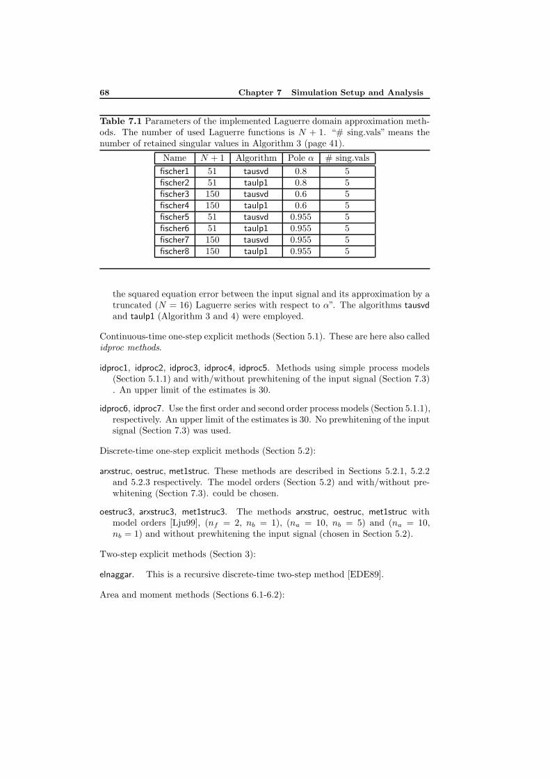
68 Chapter 7 Simulation Setup and Analysis
Table 7.1 Parameters of the implemented Laguerre domain approximation meth-ods. The number of used Laguerre functions is N + 1. “# sing.vals” means thenumber of retained singular values in Algorithm 3 (page 41).
Name N + 1 Algorithm Pole α # sing.vals
fischer1 51 tausvd 0.8 5fischer2 51 taulp1 0.8 5fischer3 150 tausvd 0.6 5fischer4 150 taulp1 0.6 5fischer5 51 tausvd 0.955 5fischer6 51 taulp1 0.955 5fischer7 150 tausvd 0.955 5fischer8 150 taulp1 0.955 5
the squared equation error between the input signal and its approximation by atruncated (N = 16) Laguerre series with respect to α”. The algorithms tausvdand taulp1 (Algorithm 3 and 4) were employed.
Continuous-time one-step explicit methods (Section 5.1). These are here also calledidproc methods.
idproc1, idproc2, idproc3, idproc4, idproc5. Methods using simple process models(Section 5.1.1) and with/without prewhitening of the input signal (Section 7.3). An upper limit of the estimates is 30.
idproc6, idproc7. Use the first order and second order process models (Section 5.1.1),respectively. An upper limit of the estimates is 30. No prewhitening of the inputsignal (Section 7.3) was used.
Discrete-time one-step explicit methods (Section 5.2):
arxstruc, oestruc, met1struc. These methods are described in Sections 5.2.1, 5.2.2and 5.2.3 respectively. The model orders (Section 5.2) and with/without pre-whitening (Section 7.3). could be chosen.
oestruc3, arxstruc3, met1struc3. The methods arxstruc, oestruc, met1struc withmodel orders [Lju99], (nf = 2, nb = 1), (na = 10, nb = 5) and (na = 10,nb = 1) and without prewhitening the input signal (chosen in Section 5.2).
Two-step explicit methods (Section 3):
elnaggar. This is a recursive discrete-time two-step method [EDE89].
Area and moment methods (Sections 6.1-6.2):
7.3 Open Loop Simulation Setup 69
area1, moment1. The area and moment methods in Sections 6.1-6.2 on estimatedstep and impulse responses (Section 4.1.2). Parameters to choose were with/without prewhitening of the input signal, two model structures (Section 6.1),and two ways to perform the numerical integration. See [Bjo03b] for details ofthe implementation.
area2, moment2. The area and moment methods using the first order model (Sec-tions 6.1-6.2) without prewhitening the input signal and certain ways to performthe numerical integration. See [Bjo03b] for implementation details.
As part of the work underlying this thesis is a Matlab function estdeadtime whichimplements some of the the time-delay estimation methods above.
7.3 Open Loop Simulation Setup
In the open loop simulations the output signal y(t) was simulated as
y(t) = G(s)u(t) + v(t) (7.1)
where u(t) and v(t) are the input and noise signals respectively. G(s) is a linearsystem with time-delay.
The factors (or conditions) of the simulations can be divided into fixed factorsand varied factors . The different possible choices for the same factor are in thisthesis called levels of the factor. The choice of level for all factors is called a factorlevel combination. A trial consists of a collection of simulations, one simulation foreach possible combination of factor levels. In factorial experiments (Section 7.1), atrial is called a replicate.
Fixed factors for the open loop simulations were: The noise v(t) was whiteand Gaussian. The system G(s) was simulated by the function lsim in [CST] incontinuous-time. The sampling interval for the time-delay estimation was Ts = 1.The varied factors for the open loop simulations are given below:
Method. The time-delay estimation methods. See Section 7.2.
Prewhite. For many of the methods in Section 7.2 the input and output signals u(t)and y(t) were either
pw. Filtered through a filter that made the input white. See Algorithm 10.
nopw. Not filtered through a prewhitening filter.
Sys. The following systems were simulated (see Figure 7.1 for impulse responses):
slow2. A slow second order system (same asG2 in Equation 4.28 in Section 4.2.6):
G1(s) = e−9s 1
(10s+ 1)(s+ 1)(7.2)
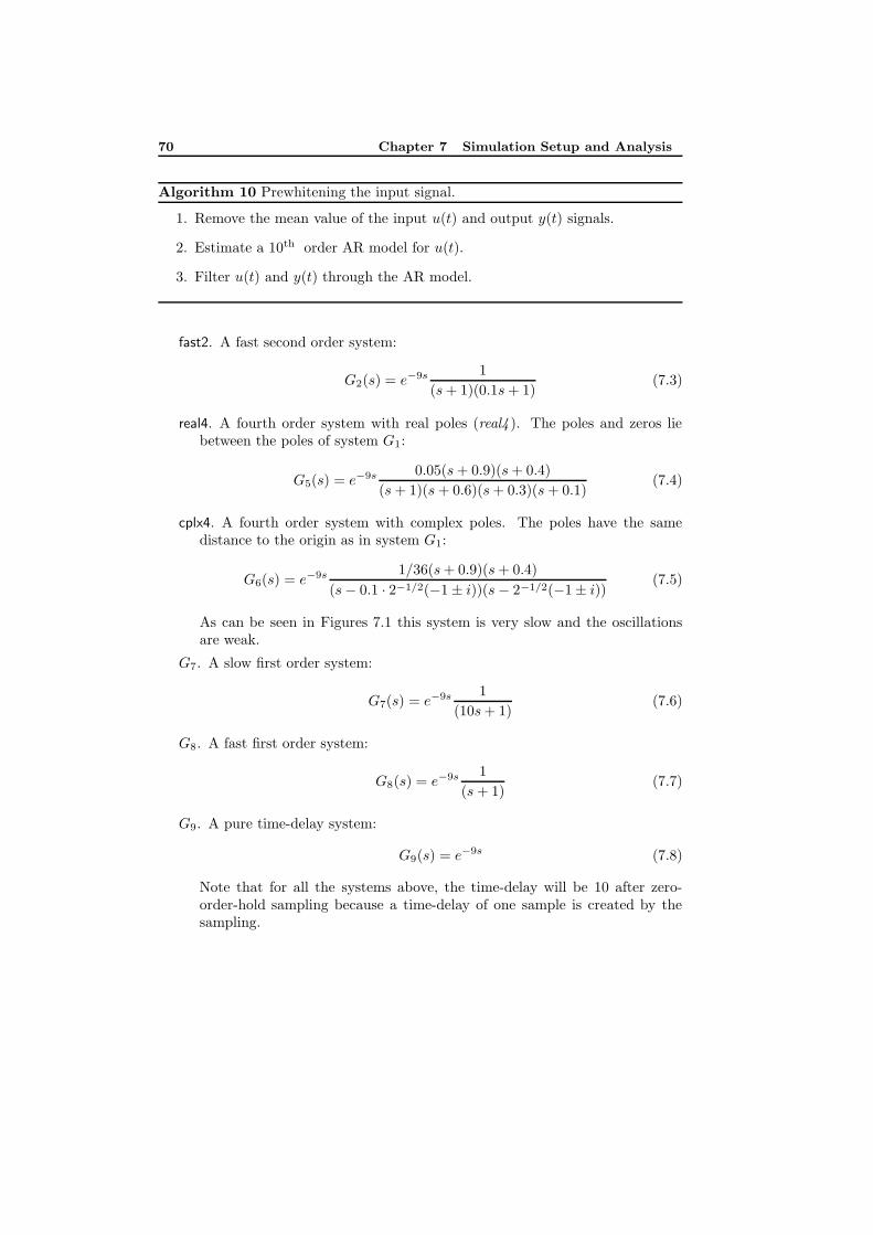
70 Chapter 7 Simulation Setup and Analysis
Algorithm 10 Prewhitening the input signal.
1. Remove the mean value of the input u(t) and output y(t) signals.
2. Estimate a 10th order AR model for u(t).
3. Filter u(t) and y(t) through the AR model.
fast2. A fast second order system:
G2(s) = e−9s 1
(s+ 1)(0.1s+ 1)(7.3)
real4. A fourth order system with real poles (real4 ). The poles and zeros liebetween the poles of system G1:
G5(s) = e−9s 0.05(s+ 0.9)(s+ 0.4)
(s+ 1)(s+ 0.6)(s+ 0.3)(s+ 0.1)(7.4)
cplx4. A fourth order system with complex poles. The poles have the samedistance to the origin as in system G1:
G6(s) = e−9s 1/36(s+ 0.9)(s+ 0.4)
(s− 0.1 · 2−1/2(−1± i))(s− 2−1/2(−1± i)) (7.5)
As can be seen in Figures 7.1 this system is very slow and the oscillationsare weak.
G7. A slow first order system:
G7(s) = e−9s 1
(10s+ 1)(7.6)
G8. A fast first order system:
G8(s) = e−9s 1
(s+ 1)(7.7)
G9. A pure time-delay system:
G9(s) = e−9s (7.8)
Note that for all the systems above, the time-delay will be 10 after zero-order-hold sampling because a time-delay of one sample is created by thesampling.
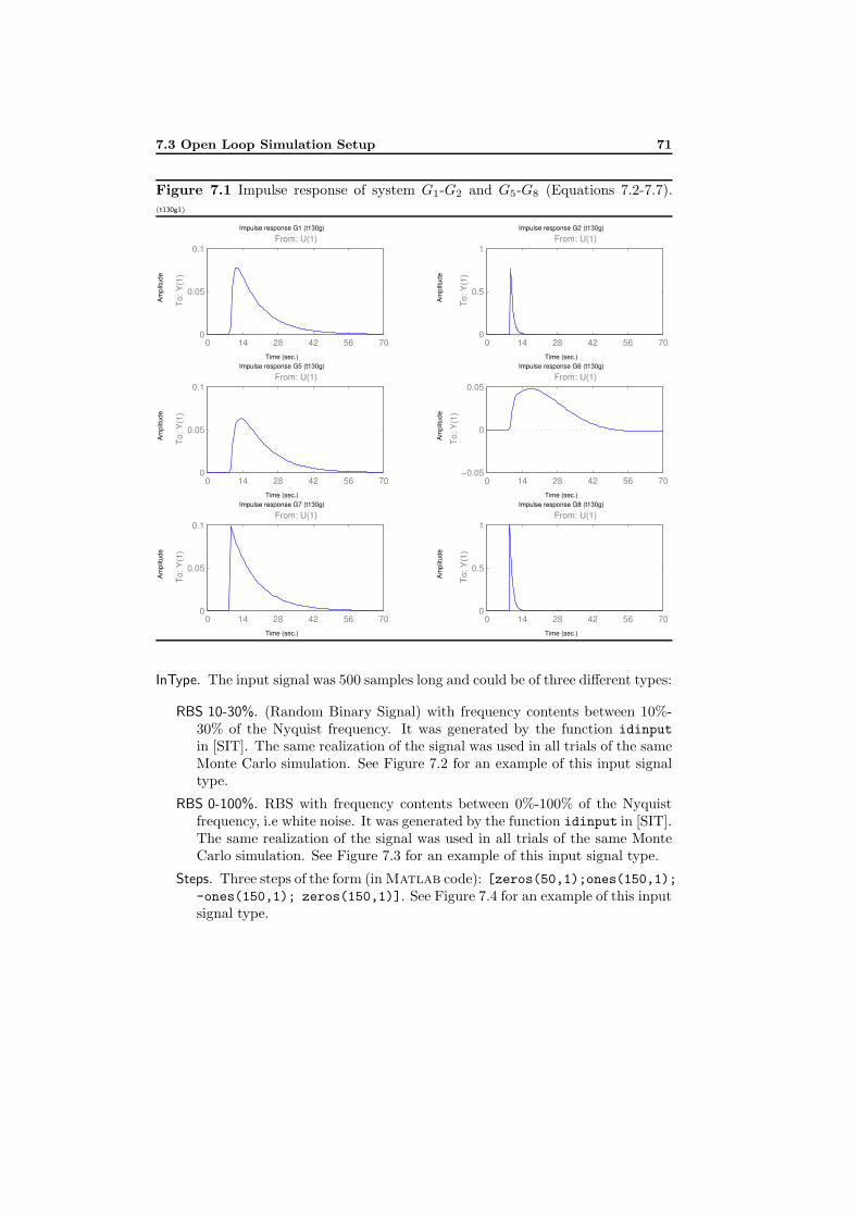
7.3 Open Loop Simulation Setup 71
Figure 7.1 Impulse response of system G1-G2 and G5-G8 (Equations 7.2-7.7).(t130g1)
Time (sec.)
Am
plitu
de
Impulse response G1 (t130g)
0 14 28 42 56 700
0.05
0.1From: U(1)
To: Y
(1)
Time (sec.)
Am
plitu
de
Impulse response G2 (t130g)
0 14 28 42 56 700
0.5
1From: U(1)
To: Y
(1)
Time (sec.)
Am
plitu
de
Impulse response G5 (t130g)
0 14 28 42 56 700
0.05
0.1From: U(1)
To: Y
(1)
Time (sec.)
Am
plitu
de
Impulse response G6 (t130g)
0 14 28 42 56 70−0.05
0
0.05From: U(1)
To: Y
(1)
Time (sec.)
Am
plitu
de
Impulse response G7 (t130g)
0 14 28 42 56 700
0.05
0.1From: U(1)
To: Y
(1)
Time (sec.)
Am
plitu
de
Impulse response G8 (t130g)
0 14 28 42 56 700
0.5
1From: U(1)
To: Y
(1)
PSfrag replacements
tu(t)y(t)s(t)
gts(t)
TdTd
δ(t− Td)g(t)gr(t)g(t)
InType. The input signal was 500 samples long and could be of three different types:
RBS 10-30%. (Random Binary Signal) with frequency contents between 10%-30% of the Nyquist frequency. It was generated by the function idinput
in [SIT]. The same realization of the signal was used in all trials of the sameMonte Carlo simulation. See Figure 7.2 for an example of this input signaltype.
RBS 0-100%. RBS with frequency contents between 0%-100% of the Nyquistfrequency, i.e white noise. It was generated by the function idinput in [SIT].The same realization of the signal was used in all trials of the same MonteCarlo simulation. See Figure 7.3 for an example of this input signal type.
Steps. Three steps of the form (in Matlab code): [zeros(50,1);ones(150,1);-ones(150,1); zeros(150,1)]. See Figure 7.4 for an example of this inputsignal type.
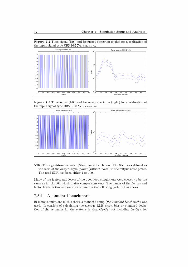
72 Chapter 7 Simulation Setup and Analysis
Figure 7.2 Time signal (left) and frequency spectrum (right) for a realization ofthe input signal type RBS 10-30%. (t160a1time, freq)
0 50 100 150 200 250 300 350 400 450 500
−1
−0.8
−0.6
−0.4
−0.2
0
0.2
0.4
0.6
0.8
1
samples
Time signal RBS10−30%
PSfrag replacements
tu(t)y(t)s(t)
gts(t)
TdTd
δ(t− Td)g(t)gr(t)g(t)
0 0.1 0.2 0.3 0.4 0.5 0.6 0.7 0.8 0.9 110−2
10−1
100
101
Normalized frequency
Pow
er
Power spectruml RBS10−30%
PSfrag replacements
tu(t)y(t)s(t)
gts(t)
TdTd
δ(t− Td)g(t)gr(t)g(t)
Figure 7.3 Time signal (left) and frequency spectrum (right) for a realization ofthe input signal type RBS 0-100%. (t160a2time, freq)
0 50 100 150 200 250 300 350 400 450 500
−1
−0.8
−0.6
−0.4
−0.2
0
0.2
0.4
0.6
0.8
1
samples
Time signal RBS0−100%
PSfrag replacements
tu(t)y(t)s(t)
gts(t)
TdTd
δ(t− Td)g(t)gr(t)g(t)
0 0.1 0.2 0.3 0.4 0.5 0.6 0.7 0.8 0.9 110−1
100
101
Normalized frequency
Pow
er
Power spectruml RBS0−100%
PSfrag replacements
tu(t)y(t)s(t)
gts(t)
TdTd
δ(t− Td)g(t)gr(t)g(t)
SNR. The signal-to-noise ratio (SNR) could be chosen. The SNR was defined asthe ratio of the output signal power (without noise) to the output noise power.The used SNR has been either 1 or 100.
Many of the factors and levels of the open loop simulations were chosen to be thesame as in [Hor00], which makes comparisons easy. The names of the factors andfactor levels in this section are also used in the following plots in this thesis.
7.3.1 A standard benchmark
In many simulations in this thesis a standard setup (the standard benchmark) wasused. It consists of calculating the average RMS error, bias or standard devia-tion of the estimates for the systems G1-G2, G5-G6 (not including G7-G9), for
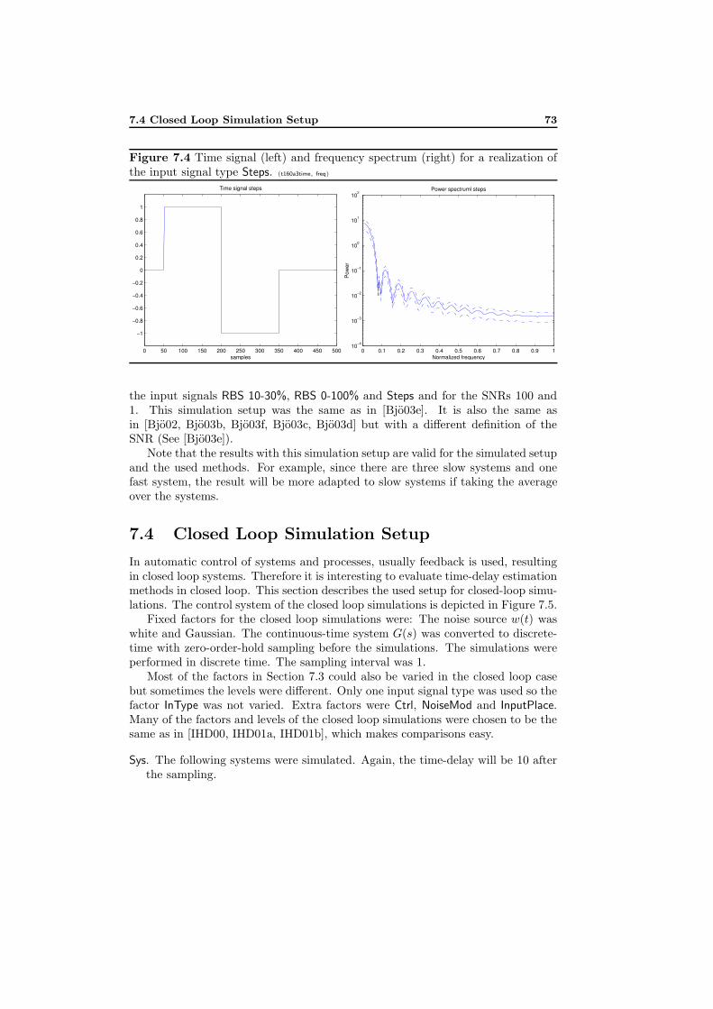
7.4 Closed Loop Simulation Setup 73
Figure 7.4 Time signal (left) and frequency spectrum (right) for a realization ofthe input signal type Steps. (t160a3time, freq)
0 50 100 150 200 250 300 350 400 450 500
−1
−0.8
−0.6
−0.4
−0.2
0
0.2
0.4
0.6
0.8
1
samples
Time signal steps
PSfrag replacements
tu(t)y(t)s(t)
gts(t)
TdTd
δ(t− Td)g(t)gr(t)g(t)
0 0.1 0.2 0.3 0.4 0.5 0.6 0.7 0.8 0.9 110−4
10−3
10−2
10−1
100
101
102
Normalized frequency
Pow
er
Power spectruml steps
PSfrag replacements
tu(t)y(t)s(t)
gts(t)
TdTd
δ(t− Td)g(t)gr(t)g(t)
the input signals RBS 10-30%, RBS 0-100% and Steps and for the SNRs 100 and1. This simulation setup was the same as in [Bjo03e]. It is also the same asin [Bjo02, Bjo03b, Bjo03f, Bjo03c, Bjo03d] but with a different definition of theSNR (See [Bjo03e]).
Note that the results with this simulation setup are valid for the simulated setupand the used methods. For example, since there are three slow systems and onefast system, the result will be more adapted to slow systems if taking the averageover the systems.
7.4 Closed Loop Simulation Setup
In automatic control of systems and processes, usually feedback is used, resultingin closed loop systems. Therefore it is interesting to evaluate time-delay estimationmethods in closed loop. This section describes the used setup for closed-loop simu-lations. The control system of the closed loop simulations is depicted in Figure 7.5.
Fixed factors for the closed loop simulations were: The noise source w(t) waswhite and Gaussian. The continuous-time system G(s) was converted to discrete-time with zero-order-hold sampling before the simulations. The simulations wereperformed in discrete time. The sampling interval was 1.
Most of the factors in Section 7.3 could also be varied in the closed loop casebut sometimes the levels were different. Only one input signal type was used so thefactor InType was not varied. Extra factors were Ctrl, NoiseMod and InputPlace.Many of the factors and levels of the closed loop simulations were chosen to be thesame as in [IHD00, IHD01a, IHD01b], which makes comparisons easy.
Sys. The following systems were simulated. Again, the time-delay will be 10 afterthe sampling.
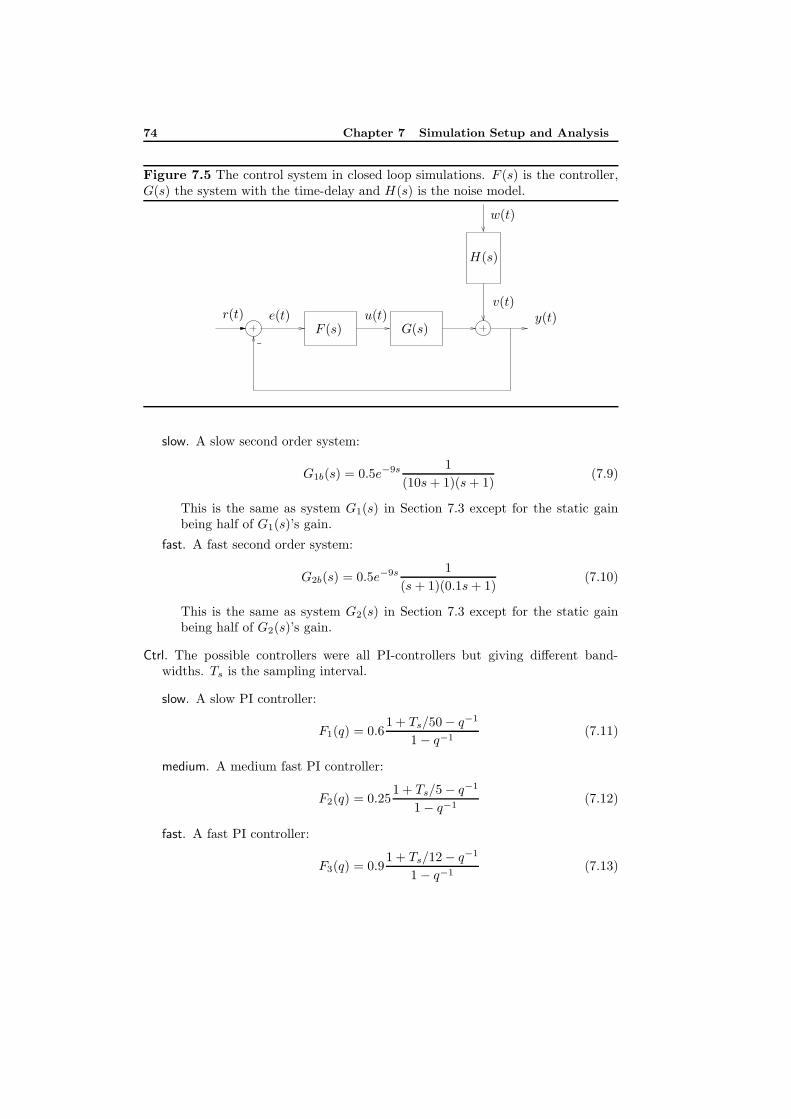
74 Chapter 7 Simulation Setup and Analysis
Figure 7.5 The control system in closed loop simulations. F (s) is the controller,G(s) the system with the time-delay and H(s) is the noise model.
−
PSfrag replacements
tu(t)y(t)s(t)
gts(t)
TdTd
δ(t− Td)g(t)gr(t)g(t)
w(t)
r(t) e(t) u(t) y(t)v(t)
H(s)
F (s) G(s)
slow. A slow second order system:
G1b(s) = 0.5e−9s 1
(10s+ 1)(s+ 1)(7.9)
This is the same as system G1(s) in Section 7.3 except for the static gainbeing half of G1(s)’s gain.
fast. A fast second order system:
G2b(s) = 0.5e−9s 1
(s+ 1)(0.1s+ 1)(7.10)
This is the same as system G2(s) in Section 7.3 except for the static gainbeing half of G2(s)’s gain.
Ctrl. The possible controllers were all PI-controllers but giving different band-widths. Ts is the sampling interval.
slow. A slow PI controller:
F1(q) = 0.61 + Ts/50− q−1
1− q−1(7.11)
medium. A medium fast PI controller:
F2(q) = 0.251 + Ts/5− q−1
1− q−1(7.12)
fast. A fast PI controller:
F3(q) = 0.91 + Ts/12− q−1
1− q−1(7.13)
7.5 Analysis Methods 75
NoiseMod. The noise model H(q) could be chosen in three different ways:
filt. White noise filtered by
H1(q) =0.71
1− 0.7q−1(7.14)
oe. Unfiltered white noise giving an output error model structure y(t) = G(q)u(t)+w(t):
H2(q) = 1 (7.15)
arx. A noise model H3(q) with the same denominator as systemG1b. This wouldgive an ARX model structure y(t) = (B(q)/A(q))u(t) + (1/A(q))w(t) withG1b except for a different normalization in the numerator of H3(q):
H3(q) =0.92
1− 0.368q−1 + 1.671 · 10−5q−2(7.16)
InType. In the closed loop simulations, only one reference signal r(t) was used. Itis here called Steps2 and consisted of two steps and 2000 samples and was gen-erated in Matlab by: [4*ones(1,1000), 2*ones(1,1000)].’. This signal isnot exactly the same as in [IHD01b] but of a similar character.
InputPlace. The input to the time-delay estimation could be either
u. The input signal u(t) to the system and the output signal y(t) or
r. The reference signal r(t) and the output signal y(t).
SNR. In the simulations the power of the noise w(t) was specified to 0.10, whichis the same as the high noise power used in [IHD00, IHD01b]. This means thatthe SNR according to our definition in Section 7.3 will be different for differentsystems and controllers. In a simulation the SNR was estimated. The maximumSNR was 1147, the minimum 790, the mean 959 and the standard deviation 66.In summary, this is a very high SNR.
7.5 Analysis Methods
In this work we have used the following analysis methods. However, the resultof not all analysis methods are shown in this thesis. There are also some specialanalysis methods that are specific to certain estimation methods. See the respectivesection about these.
1. Plots of the estimates. These give the possibility to discover outliers and seethe behavior for different factor level combinations.
76 Chapter 7 Simulation Setup and Analysis
2. Bar plots of the RMS (root mean square) error of the estimates for differentfactor level combinations. These give an estimation quality measure whichcan be used to see how good the estimates are. They also indicate whichfactor level combinations, e.g. methods, are better or worse than others. SeeSection 7.5.2.
3. Bar plots of the bias or standard deviation of the estimates for different factorlevel combinations. See Section 7.5.2.
4. ANOVA (ANalysis Of VAriance) [Mon97, Mat01] on the RMS errors for dif-ferent factor level combinations. ANOVA can tell us if there is a statisticallysignificant difference between factor level combinations, e.g. different meth-ods or systems. See Section 7.5.3.
5. Plot of confidence intervals for pair-wise comparisons [Mon97, Mat01] forthe RMS errors for different factor level combinations. This can give us thepossibility to say that certain factor level combinations, e.g. some methods,are better than others. See Section 7.5.3.
RMS error, bias and standard deviation are expressed in number of samplingintervals in this thesis. A part of the work underlying this thesis is the devel-opment of a MATLAB toolbox for managing and analyzing data from factorialexperiments [Bjo]. It uses some functions from the Matlab Statistics Tool-box [Mat01].
7.5.1 Managing failing estimates
Many methods sometimes fail and return estimates with unreasonable values (neg-ative, large positive, complex or NaN). To handle this, the following procedureswere used:
1. In this procedure, complex and NaN values and values ≤ 0 or ≥ 20 arereplaced with the value 20. This will give a large error for these estimates asthe true time-delay is 10. The maximum RMS error will also be 10. Then,the 90%, 95% or 100% best estimates are retained. Estimates of the factorlevel combinations with the worst estimates will be removed first. If somefactor level combination contain only failed estimates (RMS error =10) thenthe results in the plots will be the same for 90%, 95% and 100% as long asnot all estimates are removed from any factor level combination. This is thecase for the methods idimp5, idstep5 and idstepCusum4 in Figure 9.1. Onthe contrary, if the failed estimates are spread uniformly between factor levelcombinations, the difference between 90%, 95% and 100% will be large, aswith idproc7 in Figure 9.1.
2. In this procedure, estimates outside the region [0,20] are set to the value 20.This choice is a trade-off between how much to punish failed estimates andhow much to punish poor RMS error values when the estimates occurred.
7.5 Analysis Methods 77
It is up to the user to decide what is important. The closer this number(Td = 20) is to the correct time-delay (true Td = 10) the less punishment ofthe method for failed estimates. The more distant from correct time-delaythe more punishment for failed estimates. This can mean that dependingon the chosen punishment for failures different methods will be “best”. Thetime-delay Td = 20 is assumed to be a maximum time-delay to detect.
3. In this procedure the optimization is restricted to the region [0, 30].
The motivation for removing the worst estimates is that a good implementation ofthe estimation method can detect time-delay estimates outside an expected range([0,20] in procedure 1 above) and should be able to handle this, e.g. by restartingan optimization with a different initial value.
7.5.2 Plots of RMS error, bias and standard deviation
The computational steps for bar graphs with RMS error, bias and standard devia-tion of time-delay estimates are:
1. Optionally, remove the worst estimates. See Section 7.5.1
2. Compute the RMS error, bias or standard deviation of the time-delay esti-mates for each factor level combination separately.
3. Compute the average (or max) of the result from step 2 over the levels of thefactors which are not to be shown in the plot.
4. Plot the graph.
Thus, all results in the bar graphs are on average (or max) over all the factors thatare not explicitly studied. Certain special cases can give a different result. Alsokeep in mind that the presented RMS values only are estimates of the “true” ones.
Figure 7.6 shows an example plot. The axis label “InType*SNR” means thaton this axis there are different (factor level) combinations of input signal type andSNR. On the other axis there are different methods. The tick mark labels tell uswhat factor level combinations there are in the different “rows”and “columns”. Thelevels of the factors are separated by an asterisk “*”. For example, on the axis tothe right “steps*1”means a combination of the input signal type Steps (Section 7.3)and SNR=1. The level 10-30% is an abbreviation of RBS 10-30% and 0-100% ofRBS 0-100% . See Sections 7.3-7.4 for definitions of the factor and level names.
7.5.3 ANOVA and confidence intervals
A statistical method for analysis of experiments used in some scientific disciplinesis ANOVA (ANalysis Of VAriance) with subsequent computation of confidenceintervals for pair-wise comparisons, see for example [Mon97]. These analysis meth-ods make it possible to give statements and conclusions with a certain level ofconfidence or a specified risk of being false.
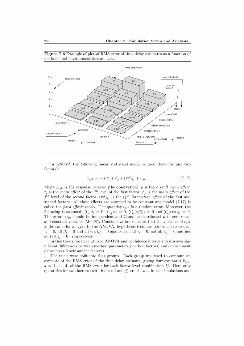
78 Chapter 7 Simulation Setup and Analysis
Figure 7.6 Example of plot of RMS error of time-delay estimates as a function ofmethods and environment factors. (t208b13)
RBS10−30%*100
RBS10−30%*1
RBS0−100%*100
RBS0−100%*1
steps*100
steps*1
oestruc3
arxstruc3
met1struc3
0
2
4
6
8
10
1.9
InType*SNR
0.67
0.45
3.7
0.063
1.8
0.44
1.2
0.0001
1.9
0.31
0.79
1.2
0.58
0.29
Method
0.15
0.52
0.2
Level of factor 1
Factor 1 Factor 3
Factor 2
Level of factor 2
Level of factor 3 RMS error axis
RMS error value
PSfrag replacements
tu(t)y(t)s(t)
gts(t)
TdTd
δ(t− Td)g(t)gr(t)g(t)
w(t)r(t)e(t)u(t)y(t)v(t)H(s)F (s)G(s)
In ANOVA the following linear statistical model is used (here for just twofactors):
xijk = µ+ τi + βj + (τβ)ij + εijk, (7.17)
where xijk is the response variable (the observation), µ is the overall mean effect,τi is the main effect of the ith level of the first factor, βj is the main effect of thejth level of the second factor, (τβ)ij is the ijth interaction effect of the first andsecond factors. All these effects are assumed to be constant and model (7.17) iscalled the fixed effects model. The quantity εijk is a random error. Moreover, thefollowing is assumed:
∑i τi = 0,
∑j βj = 0,
∑i(τβ)ij = 0 and
∑j(τβ)ij = 0.
The errors εijk should be independent and Gaussian distributed with zero meanand constant variance [Mon97]. Constant variance means that the variance of εijkis the same for all ijk. In the ANOVA, hypothesis tests are performed to test allτi = 0, all βj = 0 and all (τβ)ij = 0 against not all τi = 0, not all βj = 0 and notall (τβ)ij = 0 , respectively.
In this thesis, we have utilized ANOVA and confidence intervals to discover sig-nificant differences between method parameters (method factors) and environmentparameters (environment factors).
The trials were split into four groups. Each group was used to compute anestimate of the RMS error of the time-delay estimate, giving four estimates xijk ,k = 1, . . . , 4, of the RMS error for each factor level combination ij. Here onlyquantities for two factors (with indices i and j) are shown. In the simulations and
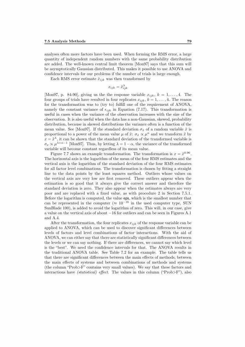
7.5 Analysis Methods 79
analyses often more factors have been used. When forming the RMS error, a largequantity of independent random numbers with the same probability distributionare added. The well-known central limit theorem [Mon97] says that this sum willbe asymptotically Gaussian distributed. This makes it possible to use ANOVA andconfidence intervals for our problems if the number of trials is large enough.
Each RMS error estimate xijk was then transformed by
xijk = xλijk
[Mon97, p. 84-90], giving us the the response variable xijk , k = 1, . . . , 4. Thefour groups of trials have resulted in four replicates xijk , k = 1, . . . , 4. The reasonfor the transformation was to (try to) fulfill one of the requirement of ANOVA,namely the constant variance of εijk in Equation (7.17). This transformation isuseful in cases when the variance of the observation increases with the size of theobservation. It is also useful when the data has a non-Gaussian, skewed, probabilitydistribution, because in skewed distributions the variance often is a function of themean value. See [Mon97]. If the standard deviation σx of a random variable x isproportional to a power of the mean value µ of x: σx ∝ µα and we transform x byx = xλ, it can be shown that the standard deviation of the transformed variable isσx ∝ µλ+α−1 [Mon97]. Thus, by letting λ = 1−α, the variance of the transformedvariable will become constant regardless of its mean value.
Figure 7.7 shows an example transformation. The transformation is x = x0.96.The horizontal axis is the logarithm of the mean of the four RMS estimates and thevertical axis is the logarithm of the standard deviation of the four RMS estimatesfor all factor level combinations. The transformation is chosen by fitting a straightline to the data points by the least squares method. Outliers whose values onthe vertical axis are very low are first removed. These outliers appear when theestimation is so good that it always give the correct answer and therefore thestandard deviation is zero. They also appear when the estimates always are verypoor and are replaced with a fixed value, as with procedure 2 in Section 7.5.1.Before the logarithm is computed, the value eps, which is the smallest number thatcan be represented in the computer (≈ 10−16 in the used computer type, SUNSunBlade 100), is added to avoid the logarithm of zero. This will, in our case, givea value on the vertical axis of about −16 for outliers and can be seen in Figures A.1and A.4.
After the transformation, the four replicates xijk of the response variable can beapplied to ANOVA, which can be used to discover significant differences betweenlevels of factors and level combinations of factor interactions. With the aid ofANOVA, we can either say that there are statistically significant differences betweenthe levels or we can say nothing. If there are differences, we cannot say which levelis the “best”. We need the confidence intervals for that. The ANOVA results inthe traditional ANOVA table. See Table 7.2 for an example. The table tells usthat there are significant differences between the main effects of methods, betweenthe main effects of systems and between combinations of methods and systems(the column “Prob>F” contains very small values). We say that these factors andinteractions have (statistical) effect. The values in this column (“Prob>F”), also
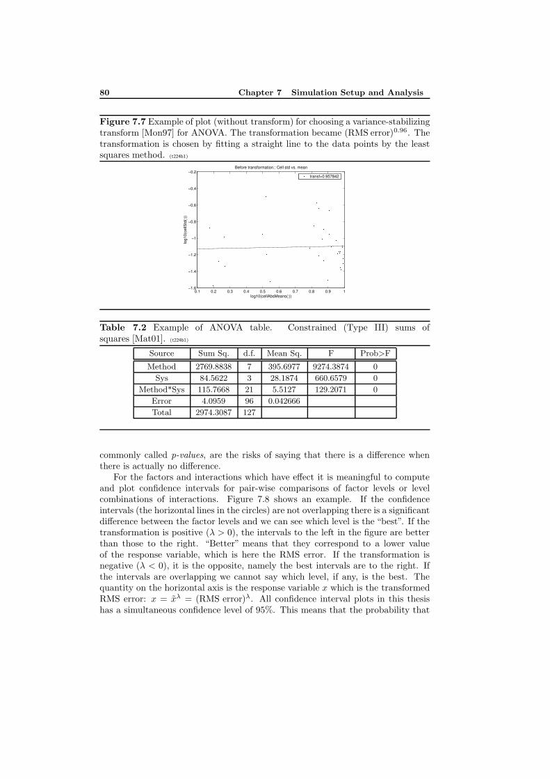
80 Chapter 7 Simulation Setup and Analysis
Figure 7.7 Example of plot (without transform) for choosing a variance-stabilizingtransform [Mon97] for ANOVA. The transformation became (RMS error)0.96. Thetransformation is chosen by fitting a straight line to the data points by the leastsquares method. (t224b1)
0.1 0.2 0.3 0.4 0.5 0.6 0.7 0.8 0.9 1−1.6
−1.4
−1.2
−1
−0.8
−0.6
−0.4
−0.2
log10(cellAbsMeans(:))
log1
0(ce
llStd
(:))
Before transformation.: Cell std vs. mean
transf=0.957842
PSfrag replacements
tu(t)y(t)s(t)
gts(t)
TdTd
δ(t− Td)g(t)gr(t)g(t)
w(t)r(t)e(t)u(t)y(t)v(t)H(s)F (s)G(s)
Table 7.2 Example of ANOVA table. Constrained (Type III) sums ofsquares [Mat01]. (t224b1)
Source Sum Sq. d.f. Mean Sq. F Prob>F
Method 2769.8838 7 395.6977 9274.3874 0
Sys 84.5622 3 28.1874 660.6579 0
Method*Sys 115.7668 21 5.5127 129.2071 0
Error 4.0959 96 0.042666
Total 2974.3087 127
commonly called p-values, are the risks of saying that there is a difference whenthere is actually no difference.
For the factors and interactions which have effect it is meaningful to computeand plot confidence intervals for pair-wise comparisons of factor levels or levelcombinations of interactions. Figure 7.8 shows an example. If the confidenceintervals (the horizontal lines in the circles) are not overlapping there is a significantdifference between the factor levels and we can see which level is the “best”. If thetransformation is positive (λ > 0), the intervals to the left in the figure are betterthan those to the right. “Better” means that they correspond to a lower valueof the response variable, which is here the RMS error. If the transformation isnegative (λ < 0), it is the opposite, namely the best intervals are to the right. Ifthe intervals are overlapping we cannot say which level, if any, is the best. Thequantity on the horizontal axis is the response variable x which is the transformedRMS error: x = xλ = (RMS error)λ. All confidence interval plots in this thesishas a simultaneous confidence level of 95%. This means that the probability that
7.5 Analysis Methods 81
all confidence intervals cover their respective parameter is 95% or with other wordsthe risk that we incorrectly say that there a difference between any of factor levelsor level combinations of interactions is 5%. Note that the horizontal lines in theplots are not confidence intervals for (µτ)i, see below.
For the reader interested in statistical details we will describe the confidenceinterval plot in Figure 7.8 in another way. We start by writing the ANOVA model(7.17) in three other forms, namely
xijk = (µτ)i + βj + (τβ)ij + εijk with (µτ)i = µ+ τi (7.18)
xijk = τi + (µβ)j + (τβ)ij + εijk with (µβ)j = µ+ βj (7.19)
xijk = µij + εijk with µij = µ+ τi + βj + (τβ)ij , (7.20)
where (µτ)i is the main mean of the ith level of the first factor, (µβ)j is the mainmean of the jth level of the second factor, µij is here called the ijth interactionmean of the first and second factors (actually, µij is the mean for the combinationof the ith level of the first factor and the jth level of the second factor in thecomplete model (7.17) where the interaction are included). We want to comparethe “means” above to see which factor levels or factor level combinations that givethe best or worst result (highest or lowest RMS error of the time-delay estimate).This can be done by computing confidence intervals for differences in the means.For example, let us assume that the interactions are negligible. If the confidenceinterval for (µτ)n− (µτ)m, where n and m correspond to different levels of the firstfactor, does not include the value zero or negative values, then the level n gives asignificant higher value of the response variable (=RMS error if no transformationis used) than the level m. Comparing all possible combinations of levels witheach other will often give very many comparisons. An economical way to performall these comparisons is utilized in the confidence interval plots in this thesis. The
circles in these plots (see Figure 7.8) mark the values of (µτ)i, i.e. estimates of (µτ)i.The horizontal lines in the circles have half the length of the confidence intervalsfor (µτ)n − (µτ)m. The confidence interval for (µτ)n − (µτ)m does not include thevalue zero exactly when the horizontal lines from neighboring circles do not overlap.The horizontal lines are not restricted to be within the circles but can sometimesextent outside the circles as in Figure 8.10. The reason for the lines being so shortin this thesis is that very many trials are used in the simulations. As already said,the horizontal lines in the plots are not confidence intervals for (µτ)i but 1/2 ofthe confidence intervals for (µτ)n − (µτ)m (with the simultaneous confidence levelof 95%). The confidence intervals in this thesis use Tukey’s honestly significantdifference criterion [Mat01]. When choosing parameters of time-delay estimationmethods, we can ourselves select the factor levels (the parameter values) and wewill study confidence intervals for (µτ)n − (µτ)m if the interactions are significant.When studying environment factors, which we cannot choose ourselves, we are oftenonly interested in how the time-delay estimation methods perform on average andstudy confidence intervals only for main means even if there are interactions thathave a statistical effect. This is somewhat unusual.
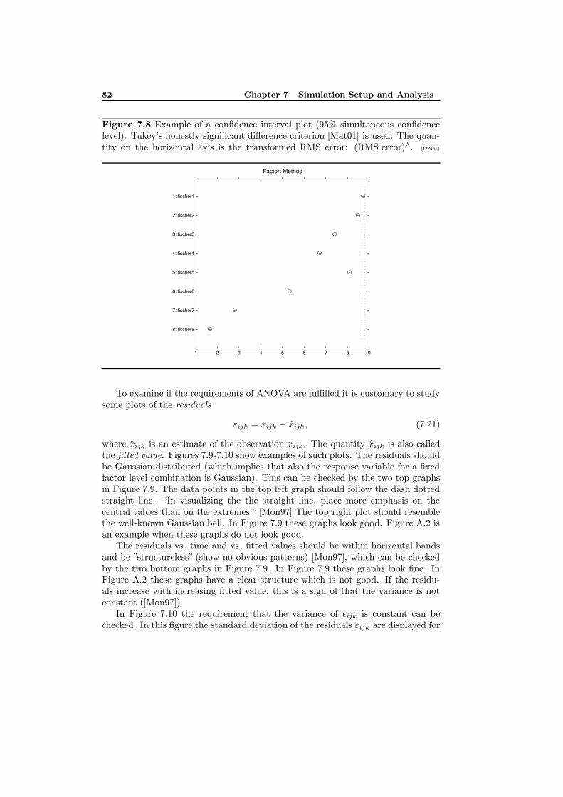
82 Chapter 7 Simulation Setup and Analysis
Figure 7.8 Example of a confidence interval plot (95% simultaneous confidencelevel). Tukey’s honestly significant difference criterion [Mat01] is used. The quan-tity on the horizontal axis is the transformed RMS error: (RMS error)λ. (t224b1)
1 2 3 4 5 6 7 8 9
8: fischer8
7: fischer7
6: fischer6
5: fischer5
4: fischer4
3: fischer3
2: fischer2
1: fischer1
Factor: Method
PSfrag replacements
tu(t)y(t)s(t)
gts(t)
TdTd
δ(t− Td)g(t)gr(t)g(t)
w(t)r(t)e(t)u(t)y(t)v(t)H(s)F (s)G(s)
To examine if the requirements of ANOVA are fulfilled it is customary to studysome plots of the residuals
εijk = xijk − xijk , (7.21)
where xijk is an estimate of the observation xijk . The quantity xijk is also calledthe fitted value. Figures 7.9-7.10 show examples of such plots. The residuals shouldbe Gaussian distributed (which implies that also the response variable for a fixedfactor level combination is Gaussian). This can be checked by the two top graphsin Figure 7.9. The data points in the top left graph should follow the dash dottedstraight line. “In visualizing the the straight line, place more emphasis on thecentral values than on the extremes.” [Mon97] The top right plot should resemblethe well-known Gaussian bell. In Figure 7.9 these graphs look good. Figure A.2 isan example when these graphs do not look good.
The residuals vs. time and vs. fitted values should be within horizontal bandsand be ”structureless” (show no obvious patterns) [Mon97], which can be checkedby the two bottom graphs in Figure 7.9. In Figure 7.9 these graphs look fine. InFigure A.2 these graphs have a clear structure which is not good. If the residu-als increase with increasing fitted value, this is a sign of that the variance is notconstant ([Mon97]).
In Figure 7.10 the requirement that the variance of εijk is constant can bechecked. In this figure the standard deviation of the residuals εijk are displayed for
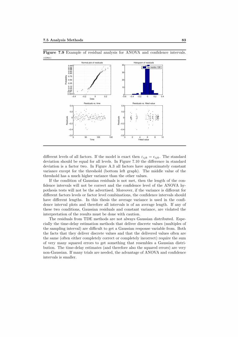
7.5 Analysis Methods 83
Figure 7.9 Example of residual analysis for ANOVA and confidence intervals.(t224b1)
−0.4 −0.2 0 0.20.0030.01 0.02 0.05 0.10 0.25
0.50
0.75 0.90 0.95 0.98 0.99 0.997
Data
Pro
babi
lity
Normal plot of residuals
−0.6 −0.4 −0.2 0 0.2 0.40
10
20
30
40Histogram of residuals
No resids=128
0 50 100 150−0.6
−0.4
−0.2
0
0.2
0.4Residuals vs. time
Time
Res
idua
ls
0 2 4 6 8 10−0.6
−0.4
−0.2
0
0.2
0.4Residuals vs. fitted value
Fitted value
Res
idua
ls
PSfrag replacements
tu(t)y(t)s(t)
gts(t)
TdTd
δ(t− Td)g(t)gr(t)g(t)
w(t)r(t)e(t)u(t)y(t)v(t)H(s)F (s)G(s)
different levels of all factors. If the model is exact then εijk = εijk . The standarddeviation should be equal for all levels. In Figure 7.10 the difference in standarddeviation is a factor two. In Figure A.3 all factors have approximately constantvariance except for the threshold (bottom left graph). The middle value of thethreshold has a much higher variance than the other values.
If the condition of Gaussian residuals is not met, then the length of the con-fidence intervals will not be correct and the confidence level of the ANOVA hy-pothesis tests will not be the advertised. Moreover, if the variance is different fordifferent factors levels or factor level combinations, the confidence intervals shouldhave different lengths. In this thesis the average variance is used in the confi-dence interval plots and therefore all intervals is of an average length. If any ofthese two conditions, Gaussian residuals and constant variance, are violated theinterpretation of the results must be done with caution.
The residuals from TDE methods are not always Gaussian distributed. Espe-cially the time-delay estimation methods that deliver discrete values (multiples ofthe sampling interval) are difficult to get a Gaussian response variable from. Boththe facts that they deliver discrete values and that the delivered values often arethe same (often either completely correct or completely incorrect) require the sumof very many squared errors to get something that resembles a Gaussian distri-bution. The time-delay estimates (and therefore also the squared errors) are verynon-Gaussian. If many trials are needed, the advantage of ANOVA and confidenceintervals is smaller.
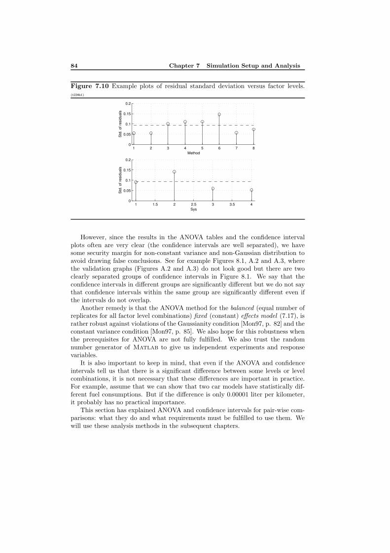
84 Chapter 7 Simulation Setup and Analysis
Figure 7.10 Example plots of residual standard deviation versus factor levels.(t224b1)
1 2 3 4 5 6 7 80
0.05
0.1
0.15
0.2
Method
Std
. of r
esid
uals
1 1.5 2 2.5 3 3.5 40
0.05
0.1
0.15
0.2
Sys
Std
. of r
esid
uals
PSfrag replacements
tu(t)y(t)s(t)
gts(t)
TdTd
δ(t− Td)g(t)gr(t)g(t)
w(t)r(t)e(t)u(t)y(t)v(t)H(s)F (s)G(s)
However, since the results in the ANOVA tables and the confidence intervalplots often are very clear (the confidence intervals are well separated), we havesome security margin for non-constant variance and non-Gaussian distribution toavoid drawing false conclusions. See for example Figures 8.1, A.2 and A.3, wherethe validation graphs (Figures A.2 and A.3) do not look good but there are twoclearly separated groups of confidence intervals in Figure 8.1. We say that theconfidence intervals in different groups are significantly different but we do not saythat confidence intervals within the same group are significantly different even ifthe intervals do not overlap.
Another remedy is that the ANOVA method for the balanced (equal number ofreplicates for all factor level combinations) fixed (constant) effects model (7.17), israther robust against violations of the Gaussianity condition [Mon97, p. 82] and theconstant variance condition [Mon97, p. 85]. We also hope for this robustness whenthe prerequisites for ANOVA are not fully fulfilled. We also trust the randomnumber generator of Matlab to give us independent experiments and responsevariables.
It is also important to keep in mind, that even if the ANOVA and confidenceintervals tell us that there is a significant difference between some levels or levelcombinations, it is not necessary that these differences are important in practice.For example, assume that we can show that two car models have statistically dif-ferent fuel consumptions. But if the difference is only 0.00001 liter per kilometer,it probably has no practical importance.
This section has explained ANOVA and confidence intervals for pair-wise com-parisons: what they do and what requirements must be fulfilled to use them. Wewill use these analysis methods in the subsequent chapters.
8Parameters and Properties of
Time-Delay Estimation Methods
In this Chapter, parameters in time-delay estimation (TDE) methods are chosenby analysis of Monte Carlo simulations to optimize their estimation quality. Also,some properties of different classes of TDE methods are observed. The sections inthis chapter follow the classification given in Chapter 3.
8.1 Time Domain Approximation Methods
In this section we will choose parameters and study properties of the time do-main approximation methods idimp4, idstep4, idimpCusum3 and idstepCusum3 (Sec-tion 7.2). These methods can also be called thresholding methods.
8.1.1 Choosing parameters in thresholding methods
Here we will show how we can choose the the relative threshold hstd and with/with-out prewhitening in the method idimp4 in Section 7.2. Some simple experimentsshowed that it is difficult to manually select method parameters that are suitablefor all cases (all level combinations of the environment factors input signal type andSNR). Therefore, the parameters are chosen with the help of confidence intervals.Often the methods miss to detect and fail to deliver an estimate [Bjo03b]). In suchcases procedure 2 in Section 7.5.1 is employed.
In the ANOVA table, Table A.1, the p-value (Section 7.5.3) for prewhiteningis 0.053, which is a rather low risk for saying that there is a difference when thereis no. However, since the prerequisites of the ANOVA (Figures A.2A.3) seem notto be fulfilled we cannot say that there is any difference between with and without
85
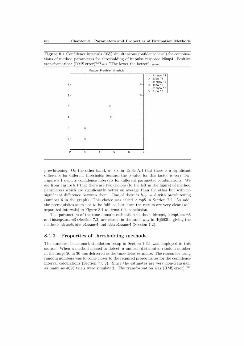
86 Chapter 8 Parameters and Properties of Estimation Methods
Figure 8.1 Confidence intervals (95% simultaneous confidence level) for combina-tions of method parameters for thresholding of impulse response idimp4. Positivetransformation: (RMS error)0.91=> ”The lower the better”. (t228b4)
2 3 4 5 6 7
6
5
4
3
2
1
Factors: Prewhite * threshold
1: nopw * 12: pw * 1 3: nopw * 34: pw * 3 5: nopw * 56: pw * 5
PSfrag replacements
tu(t)y(t)s(t)
gts(t)
TdTd
δ(t− Td)g(t)gr(t)g(t)
w(t)r(t)e(t)u(t)y(t)v(t)H(s)F (s)G(s)
prewhitening. On the other hand, we see in Table A.1 that there is a significantdifference for different thresholds because the p-value for this factor is very low.Figure 8.1 depicts confidence intervals for different parameter combinations. Wesee from Figure 8.1 that there are two choices (to the left in the figure) of methodparameters which are significantly better on average than the other but with nosignificant difference between them. One of these is hstd = 5 with prewhitening(number 6 in the graph). This choice was called idimp5 in Section 7.2. As said,the prerequisites seem not to be fulfilled but since the results are very clear (wellseparated intervals) in Figure 8.1 we trust this conclusion.
The parameters of the time domain estimation methods idstep4, idimpCusum3and idstepCusum3 (Section 7.2) are chosen in the same way in [Bjo03b], giving themethods idstep5, idimpCusum4 and idstepCusum4 (Section 7.2).
8.1.2 Properties of thresholding methods
The standard benchmark simulation setup in Section 7.3.1 was employed in thissection. When a method missed to detect, a uniform distributed random numberin the range 20 to 30 was delivered as the time-delay estimate. The reason for usingrandom numbers was to come closer to the required prerequisites for the confidenceinterval calculations (Section 7.5.3). Since the estimates are very non-Gaussian,as many as 4096 trials were simulated. The transformation was (RMS error)0.89
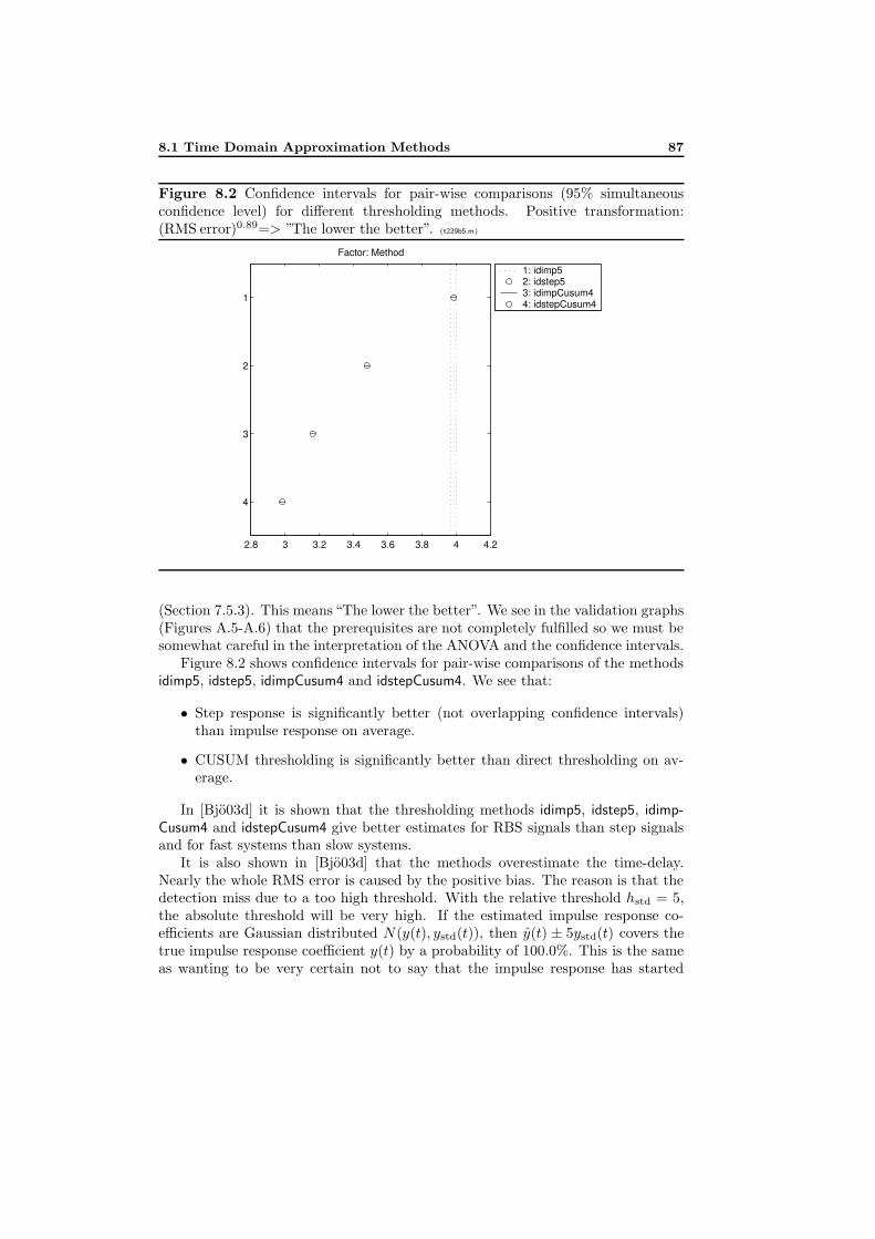
8.1 Time Domain Approximation Methods 87
Figure 8.2 Confidence intervals for pair-wise comparisons (95% simultaneousconfidence level) for different thresholding methods. Positive transformation:(RMS error)0.89=> ”The lower the better”. (t229b5.m)
2.8 3 3.2 3.4 3.6 3.8 4 4.2
4
3
2
1
Factor: Method
1: idimp5 2: idstep5 3: idimpCusum4 4: idstepCusum4
PSfrag replacements
tu(t)y(t)s(t)
gts(t)
TdTd
δ(t− Td)g(t)gr(t)g(t)
w(t)r(t)e(t)u(t)y(t)v(t)H(s)F (s)G(s)
(Section 7.5.3). This means“The lower the better”. We see in the validation graphs(Figures A.5-A.6) that the prerequisites are not completely fulfilled so we must besomewhat careful in the interpretation of the ANOVA and the confidence intervals.
Figure 8.2 shows confidence intervals for pair-wise comparisons of the methodsidimp5, idstep5, idimpCusum4 and idstepCusum4. We see that:
• Step response is significantly better (not overlapping confidence intervals)than impulse response on average.
• CUSUM thresholding is significantly better than direct thresholding on av-erage.
In [Bjo03d] it is shown that the thresholding methods idimp5, idstep5, idimp-Cusum4 and idstepCusum4 give better estimates for RBS signals than step signalsand for fast systems than slow systems.
It is also shown in [Bjo03d] that the methods overestimate the time-delay.Nearly the whole RMS error is caused by the positive bias. The reason is that thedetection miss due to a too high threshold. With the relative threshold hstd = 5,the absolute threshold will be very high. If the estimated impulse response co-efficients are Gaussian distributed N(y(t), ystd(t)), then y(t) ± 5ystd(t) covers thetrue impulse response coefficient y(t) by a probability of 100.0%. This is the sameas wanting to be very certain not to say that the impulse response has started
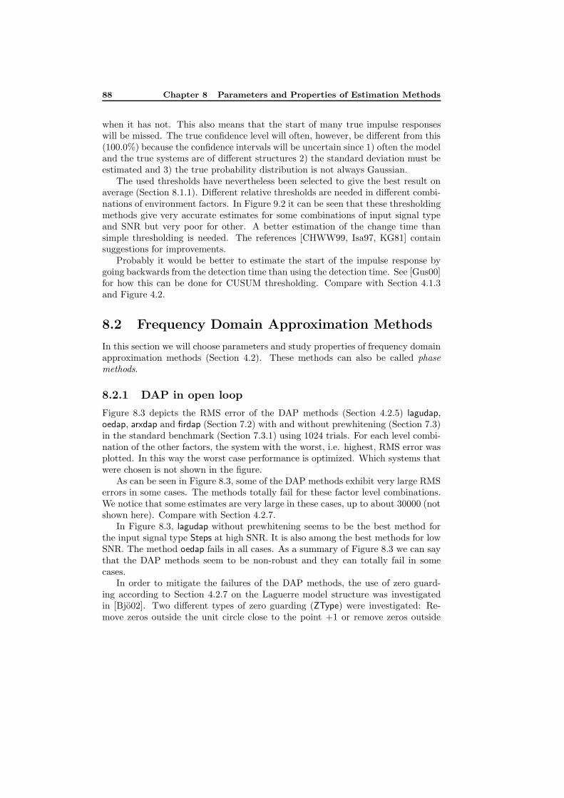
88 Chapter 8 Parameters and Properties of Estimation Methods
when it has not. This also means that the start of many true impulse responseswill be missed. The true confidence level will often, however, be different from this(100.0%) because the confidence intervals will be uncertain since 1) often the modeland the true systems are of different structures 2) the standard deviation must beestimated and 3) the true probability distribution is not always Gaussian.
The used thresholds have nevertheless been selected to give the best result onaverage (Section 8.1.1). Different relative thresholds are needed in different combi-nations of environment factors. In Figure 9.2 it can be seen that these thresholdingmethods give very accurate estimates for some combinations of input signal typeand SNR but very poor for other. A better estimation of the change time thansimple thresholding is needed. The references [CHWW99, Isa97, KG81] containsuggestions for improvements.
Probably it would be better to estimate the start of the impulse response bygoing backwards from the detection time than using the detection time. See [Gus00]for how this can be done for CUSUM thresholding. Compare with Section 4.1.3and Figure 4.2.
8.2 Frequency Domain Approximation Methods
In this section we will choose parameters and study properties of frequency domainapproximation methods (Section 4.2). These methods can also be called phasemethods.
8.2.1 DAP in open loop
Figure 8.3 depicts the RMS error of the DAP methods (Section 4.2.5) lagudap,oedap, arxdap and firdap (Section 7.2) with and without prewhitening (Section 7.3)in the standard benchmark (Section 7.3.1) using 1024 trials. For each level combi-nation of the other factors, the system with the worst, i.e. highest, RMS error wasplotted. In this way the worst case performance is optimized. Which systems thatwere chosen is not shown in the figure.
As can be seen in Figure 8.3, some of the DAP methods exhibit very large RMSerrors in some cases. The methods totally fail for these factor level combinations.We notice that some estimates are very large in these cases, up to about 30000 (notshown here). Compare with Section 4.2.7.
In Figure 8.3, lagudap without prewhitening seems to be the best method forthe input signal type Steps at high SNR. It is also among the best methods for lowSNR. The method oedap fails in all cases. As a summary of Figure 8.3 we can saythat the DAP methods seem to be non-robust and they can totally fail in somecases.
In order to mitigate the failures of the DAP methods, the use of zero guard-ing according to Section 4.2.7 on the Laguerre model structure was investigatedin [Bjo02]. Two different types of zero guarding (ZType) were investigated: Re-move zeros outside the unit circle close to the point +1 or remove zeros outside
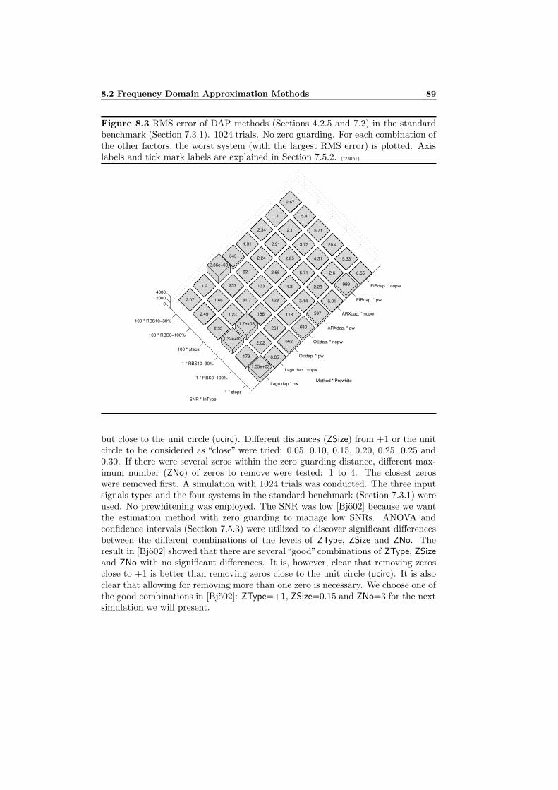
8.2 Frequency Domain Approximation Methods 89
Figure 8.3 RMS error of DAP methods (Sections 4.2.5 and 7.2) in the standardbenchmark (Section 7.3.1). 1024 trials. No zero guarding. For each combination ofthe other factors, the worst system (with the largest RMS error) is plotted. Axislabels and tick mark labels are explained in Section 7.5.2. (t230b1)
100 * RBS10−30%
100 * RBS0−100%
100 * steps
1 * RBS10−30%
1 * RBS0−100%
1 * steps
FIRdap. * nopw
FIRdap. * pw
ARXdap. * nopw
ARXdap. * pw
OEdap. * nopw
OEdap. * pw
Lagu.dap * nopw
Lagu.dap * pw
020004000
6.55
5.33
999
20.4
2.6
6.91
5.71
4.31
2.28
597
Method * Prewhite
5.4
3.73
5.71
3.14
680
2.67
2.1
2.85
4.3
118
662
1.1
2.91
2.66
128
261
6.85
2.34
2.24
133
186
2.02
1.55e+03
1.31
62.1
81.7
1.7e+03
179
643
257
1.23
1.32e+03
2.36e+03
1.66
2.33
SNR * InType
1.2
2.49
2.07
PSfrag replacements
tu(t)y(t)s(t)
gts(t)
TdTd
δ(t− Td)g(t)gr(t)g(t)
w(t)r(t)e(t)u(t)y(t)v(t)H(s)F (s)G(s)
but close to the unit circle (ucirc). Different distances (ZSize) from +1 or the unitcircle to be considered as “close” were tried: 0.05, 0.10, 0.15, 0.20, 0.25, 0.25 and0.30. If there were several zeros within the zero guarding distance, different max-imum number (ZNo) of zeros to remove were tested: 1 to 4. The closest zeroswere removed first. A simulation with 1024 trials was conducted. The three inputsignals types and the four systems in the standard benchmark (Section 7.3.1) wereused. No prewhitening was employed. The SNR was low [Bjo02] because we wantthe estimation method with zero guarding to manage low SNRs. ANOVA andconfidence intervals (Section 7.5.3) were utilized to discover significant differencesbetween the different combinations of the levels of ZType, ZSize and ZNo. Theresult in [Bjo02] showed that there are several “good”combinations of ZType, ZSizeand ZNo with no significant differences. It is, however, clear that removing zerosclose to +1 is better than removing zeros close to the unit circle (ucirc). It is alsoclear that allowing for removing more than one zero is necessary. We choose one ofthe good combinations in [Bjo02]: ZType=+1, ZSize=0.15 and ZNo=3 for the nextsimulation we will present.
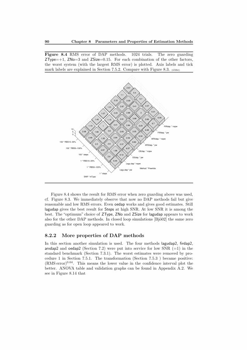
90 Chapter 8 Parameters and Properties of Estimation Methods
Figure 8.4 RMS error of DAP methods. 1024 trials. The zero guardingZType=+1, ZNo=3 and ZSize=0.15. For each combination of the other factors,the worst system (with the largest RMS error) is plotted. Axis labels and tickmark labels are explained in Section 7.5.2. Compare with Figure 8.3. (t232b1)
100 * RBS10−30%
100 * RBS0−100%
100 * steps
1 * RBS10−30%
1 * RBS0−100%
1 * steps
FIRdap. * nopw
FIRdap. * pw
ARXdap. * nopw
ARXdap. * pw
OEdap. * nopw
OEdap. * pw
Lagu.dap * nopw
Lagu.dap * pw
05
10
6.06
5.31
6.7
4.37
2.66
6.08
5.7
3
2.23
6.34
Method * Prewhite
5.4
3.41
3.98
3.05
6.84
2.67
2.09
2.88
2.84
2.59
6.57
1.1
2.87
2.61
2.65
2.37
6.12
2.33
2.23
3.41
2.94
1.96
6.45
1.31
1.15
3.8
2.9
2.6
1.07
1
1.26
2.87
1.45
1.66
2.3
SNR * InType
1.19
2.49
2.08
PSfrag replacements
tu(t)y(t)s(t)
gts(t)
TdTd
δ(t− Td)g(t)gr(t)g(t)
w(t)r(t)e(t)u(t)y(t)v(t)H(s)F (s)G(s)
Figure 8.4 shows the result for RMS error when zero guarding above was used,cf. Figure 8.3. We immediately observe that now no DAP methods fail but givereasonable and low RMS errors. Even oedap works and gives good estimates. Stilllagudap gives the best result for Steps at high SNR. At low SNR it is among thebest. The “optimum” choice of ZType, ZNo and ZSize for lagudap appears to workalso for the other DAP methods. In closed loop simulations [Bjo02] the same zeroguarding as for open loop appeared to work.
8.2.2 More properties of DAP methods
In this section another simulation is used. The four methods lagudap2, firdap2,arxdap2 and oedap2 (Section 7.2) were put into service for low SNR (=1) in thestandard benchmark (Section 7.3.1). The worst estimates were removed by pro-cedure 1 in Section 7.5.1. The transformation (Section 7.5.3 ) became positive:(RMS error)0.64. This means the lower value in the confidence interval plot thebetter. ANOVA table and validation graphs can be found in Appendix A.2. Wesee in Figure 8.14 that
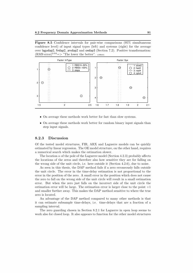
8.2 Frequency Domain Approximation Methods 91
Figure 8.5 Confidence intervals for pair-wise comparisons (95% simultaneousconfidence level) of input signal types (left) and systems (right) for the averageover lagudap2, firdap2, arxdap2 and oedap3 (Section 7.2). Positive transformation:(RMS error)0.64=> ”The lower the better”. (t208b16)
1.5 2 2.5
3
2
1
Factor: InType
1: RBS10−30%2: RBS0−100%3: steps
PSfrag replacements
tu(t)y(t)s(t)
gts(t)
TdTd
δ(t− Td)g(t)gr(t)g(t)
w(t)r(t)e(t)u(t)y(t)v(t)H(s)F (s)G(s)
1.6 1.7 1.8 1.9 2 2.1
4
3
2
1
Factor: Sys
1: slow22: fast23: real44: cplx4
PSfrag replacements
tu(t)y(t)s(t)
gts(t)
TdTd
δ(t− Td)g(t)gr(t)g(t)
w(t)r(t)e(t)u(t)y(t)v(t)H(s)F (s)G(s)
• On average these methods work better for fast than slow systems.
• On average these methods work better for random binary input signals thanstep input signals.
8.2.3 Discussion
Of the tested model structures, FIR, ARX and Laguerre models can be quicklyestimated by linear regression. The OE model structure, on the other hand, requiresa numerical search which makes the estimation slower.
The location α of the pole of the Laguerre model (Section 4.2.3) probably affectsthe locations of the zeros and therefore also how sensitive they are for falling onthe wrong side of the unit circle, i.e. here outside it (Section 4.2.6), due to noise.
As seen in this thesis, the DAP method fails if a zero erroneously falls outsidethe unit circle. The error in the time-delay estimation is not proportional to theerror in the position of the zero. A small error in the position which does not causethe zero to fall on the wrong side of the unit circle will result in a small estimationerror. But when the zero just falls on the incorrect side of the unit circle theestimation error will be large. The estimation error is larger close to the point +1and smaller further away. This makes the DAP method sensitive to where the truezero is located.
An advantage of the DAP method compared to many other methods is thatit can estimate subsample time-delays, i.e. time-delays that are a fraction of asampling interval.
The zero guarding chosen in Section 8.2.1 for Laguerre in open loop seems towork also for closed loop. It also appears to function for the other model structures
92 Chapter 8 Parameters and Properties of Estimation Methods
in both open loop and closed loop. Thus, the choice of zero guarding appears tobe robust.
In Section 8.2.1 we saw that sometimes it is not enough to remove only onezero. The reason is likely that because complex zeros come in complex conjugatedpairs, both zeros in the pair must be removed.
The location of the true non-minimum phase zeros probably depends on thetime-delay and the sampling interval. The longer time-delay or the shorter samplinginterval, the closer to the point +1 will the true zeros be. Therefore ZSize dependson the maximum possible time-delay and on the sampling interval.
A reason why Laguerre DAP works well for step input signals could be as follows.It is well known that an estimated model will become better in frequency rangeswhere the input signal has much energy [Lju99]. Since a step-like input signal hasits most energy at the frequencies which are used by the time-delay estimation, i.eat low frequencies, it will result in a good time-delay estimate.
In the open-loop simulations the fast second order system gave the lowest RMSerror on average. This is natural because this system exhibits a clearer start of therise in the step response. The fourth order system with complex poles gave thehighest RMS error on average. It seems that a more complex system makes thetime-delay estimation more difficult.
For step signals in open and closed loop, we in this thesis agree with [Hor00,IHD01b] that Laguerre DAP is a suitable estimation method. [Hor00, IHD01b]have, however, only tested with step signals and not reported that the DAP methodsometimes fails.
8.2.4 Conclusions
We draw the following conclusions from our work on DAP methods:
• The DAP method is not restricted to the Laguerre model structure but canbe used with any linear model structure, e.g. OE, ARX or FIR.
• DAP methods are inherently non-robust and can totally fail in some cases.
• The probability of failure of a DAP method depends on the model structureof the estimated model, the input signal type and the SNR.
• In failing cases, DAP methods can be made more robust by zero guarding. Ameans to choose the zero guarding for a certain application is using confidenceintervals on estimates from simulated signals.
• An appropriate choice of zero guarding appears to be robust and work forseveral model structures in both open loop and closed loop.
• For zero guarding of Laguerre DAP, removing zeros outside the unit circleclose to +1 works better than removing zeros at other places outside butclose to the unit circle. We must also allow more than one zero (a complexconjugated pair) to be removed.
8.3 Laguerre Domain Approximation Methods 93
• Most often the DAP methods work better without prewhitening the data.
• OE DAP requires much more computation time than FIR, ARX or LaguerreDAP. See also Section 9.4.
8.3 Laguerre Domain Approximation Methods
In this section we will choose parameters and study properties of Laguerre domainapproximation methods (Section 4.3).
8.3.1 The standard benchmark
We use the standard simulation setup in Section 7.3.1. Before the analysis methodsare employed, outliers and failed estimates have been removed by procedure 1 inSection 7.5.1 .
Figure 8.6 displays the RMS error for combinations of method and input signaltype. By comparing Figure 8.6 with other RMS error plots in this thesis, e.g.Figure 9.1, the following conclusions are drawn:
• Step input signals are possible to use but RBS signals are not.
• For step input signals, the method fischer8 seems to be the best.
8.3.2 Several Laguerre domain approximation methods withstep input
We now restrict ourselves to step signals and compare the different Laguerre do-main approximation methods with the aid of confidence intervals for pair-wisecomparisons.
We use the estimates for the low SNR (SNR=1). The number of trials was 1152.Outliers and failed estimates have been removed by procedure 1 in Section 7.5.1.The ANOVA table [Bjo03e] shows that there are significant differences betweencombinations of methods and systems. The confidence interval plot in Figure 8.7shows that fischer8 indeed is significantly better than the other methods for stepinput. The validation graphs for the use of ANOVA and the confidence intervalplot in Appendix A.3.1 look very fine.
When using high SNR (SNR=100), the prerequisites for the ANOVA and theconfidence interval plot were not fulfilled (determined by the same type of graphsas in Appendix A.3.1). Since the case with low SNR is a more difficult case thanwith high SNR, we consider it to be more informative. It must be more difficult fora method to be best for low SNR. It should then not be bad for high SNR either.
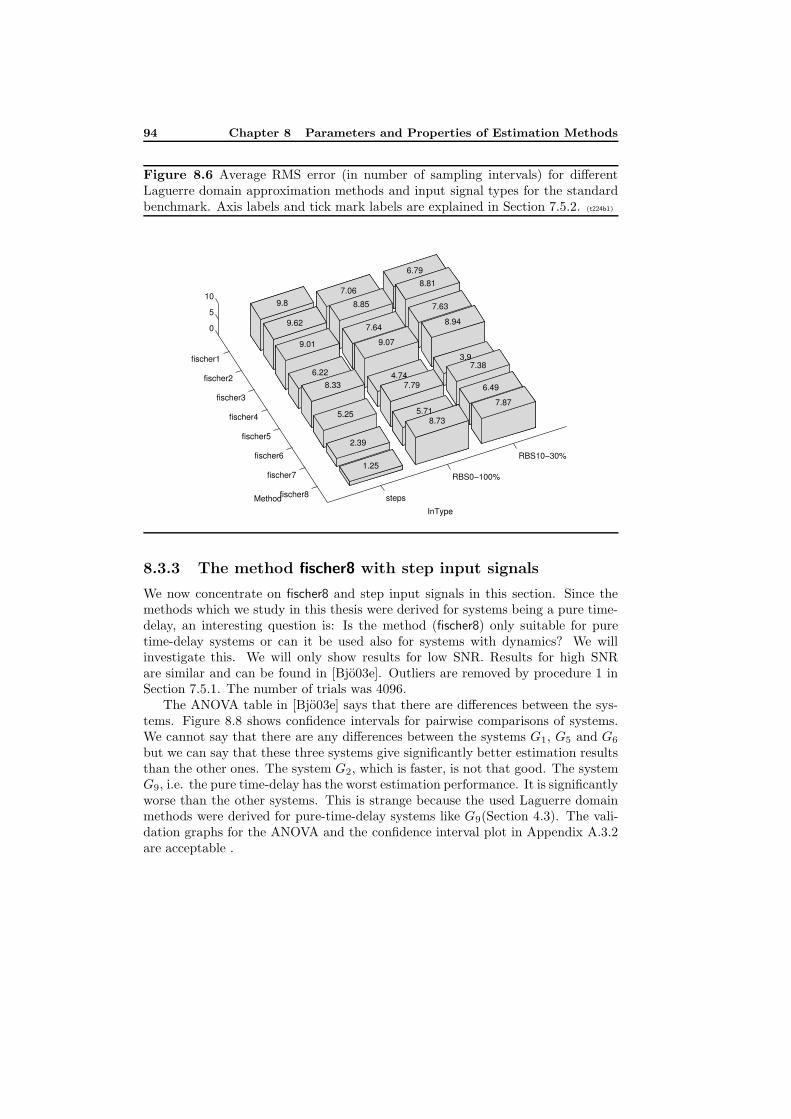
94 Chapter 8 Parameters and Properties of Estimation Methods
Figure 8.6 Average RMS error (in number of sampling intervals) for differentLaguerre domain approximation methods and input signal types for the standardbenchmark. Axis labels and tick mark labels are explained in Section 7.5.2. (t224b1)
RBS10−30%
RBS0−100%
steps
fischer1
fischer2
fischer3
fischer4
fischer5
fischer6
fischer7
fischer8
0
5
10
7.87
6.49
7.383.9
8.94
7.63
8.73
InType
8.81
5.71
6.79
7.794.74
9.07
7.64
1.25
8.85
2.39
7.06
5.25
8.336.22
9.01
9.62
9.8
Method
PSfrag replacements
tu(t)y(t)s(t)
gts(t)
TdTd
δ(t− Td)g(t)gr(t)g(t)
w(t)r(t)e(t)u(t)y(t)v(t)H(s)F (s)G(s)
8.3.3 The method fischer8 with step input signals
We now concentrate on fischer8 and step input signals in this section. Since themethods which we study in this thesis were derived for systems being a pure time-delay, an interesting question is: Is the method (fischer8) only suitable for puretime-delay systems or can it be used also for systems with dynamics? We willinvestigate this. We will only show results for low SNR. Results for high SNRare similar and can be found in [Bjo03e]. Outliers are removed by procedure 1 inSection 7.5.1. The number of trials was 4096.
The ANOVA table in [Bjo03e] says that there are differences between the sys-tems. Figure 8.8 shows confidence intervals for pairwise comparisons of systems.We cannot say that there are any differences between the systems G1, G5 and G6
but we can say that these three systems give significantly better estimation resultsthan the other ones. The system G2, which is faster, is not that good. The systemG9, i.e. the pure time-delay has the worst estimation performance. It is significantlyworse than the other systems. This is strange because the used Laguerre domainmethods were derived for pure-time-delay systems like G9(Section 4.3). The vali-dation graphs for the ANOVA and the confidence interval plot in Appendix A.3.2are acceptable .
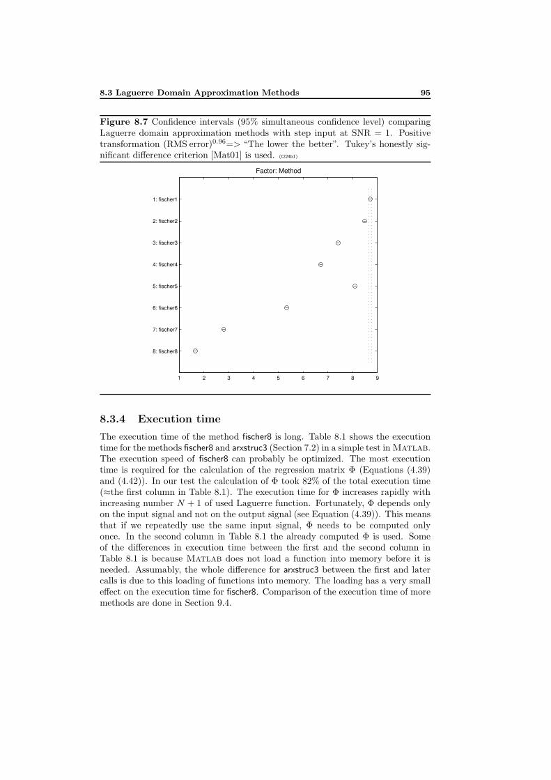
8.3 Laguerre Domain Approximation Methods 95
Figure 8.7 Confidence intervals (95% simultaneous confidence level) comparingLaguerre domain approximation methods with step input at SNR = 1. Positivetransformation (RMS error)0.96=> “The lower the better”. Tukey’s honestly sig-nificant difference criterion [Mat01] is used. (t224b1)
1 2 3 4 5 6 7 8 9
8: fischer8
7: fischer7
6: fischer6
5: fischer5
4: fischer4
3: fischer3
2: fischer2
1: fischer1
Factor: Method
PSfrag replacements
tu(t)y(t)s(t)
gts(t)
TdTd
δ(t− Td)g(t)gr(t)g(t)
w(t)r(t)e(t)u(t)y(t)v(t)H(s)F (s)G(s)
8.3.4 Execution time
The execution time of the method fischer8 is long. Table 8.1 shows the executiontime for the methods fischer8 and arxstruc3 (Section 7.2) in a simple test in Matlab.The execution speed of fischer8 can probably be optimized. The most executiontime is required for the calculation of the regression matrix Φ (Equations (4.39)and (4.42)). In our test the calculation of Φ took 82% of the total execution time(≈the first column in Table 8.1). The execution time for Φ increases rapidly withincreasing number N + 1 of used Laguerre function. Fortunately, Φ depends onlyon the input signal and not on the output signal (see Equation (4.39)). This meansthat if we repeatedly use the same input signal, Φ needs to be computed onlyonce. In the second column in Table 8.1 the already computed Φ is used. Someof the differences in execution time between the first and the second column inTable 8.1 is because Matlab does not load a function into memory before it isneeded. Assumably, the whole difference for arxstruc3 between the first and latercalls is due to this loading of functions into memory. The loading has a very smalleffect on the execution time for fischer8. Comparison of the execution time of moremethods are done in Section 9.4.
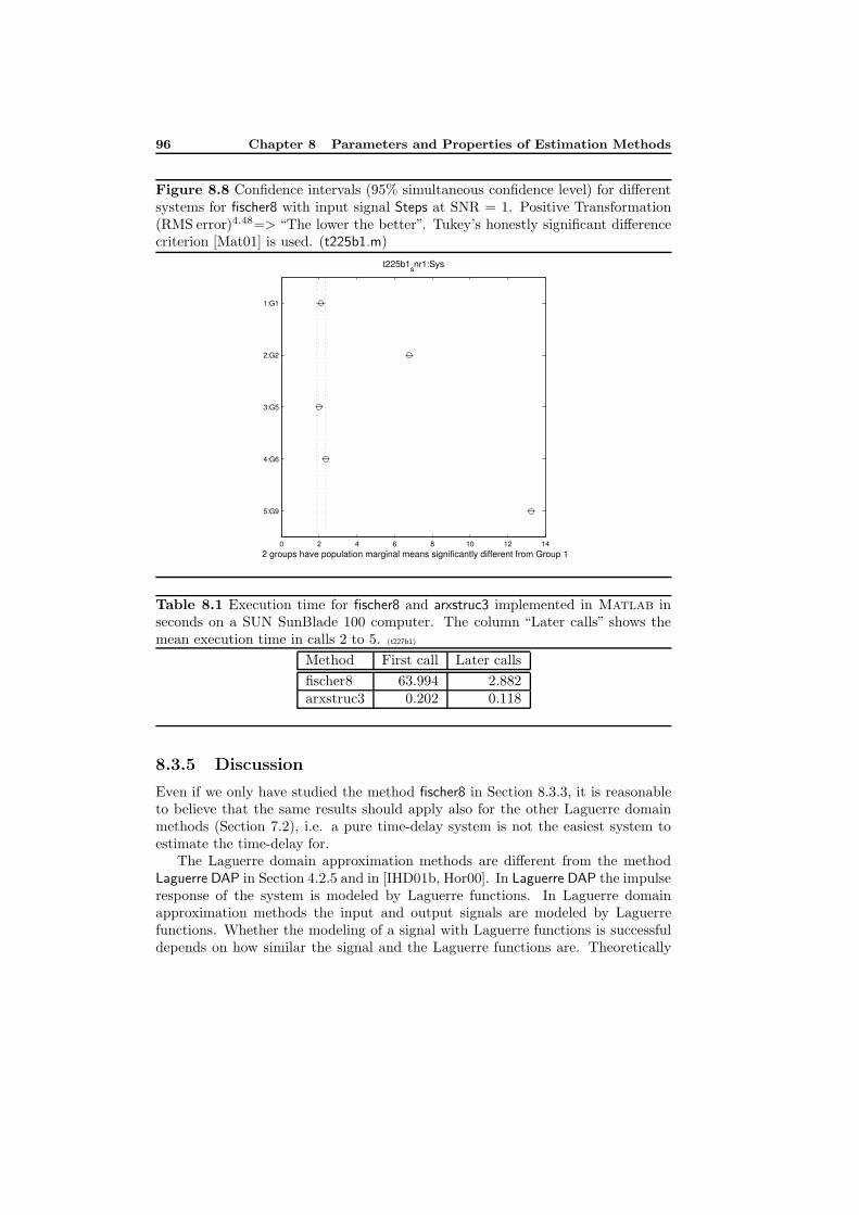
96 Chapter 8 Parameters and Properties of Estimation Methods
Figure 8.8 Confidence intervals (95% simultaneous confidence level) for differentsystems for fischer8 with input signal Steps at SNR = 1. Positive Transformation(RMS error)4.48=> “The lower the better”. Tukey’s honestly significant differencecriterion [Mat01] is used. (t225b1.m)
0 2 4 6 8 10 12 14
5:G9
4:G6
3:G5
2:G2
1:G1
t225b1snr1:Sys
2 groups have population marginal means significantly different from Group 1
PSfrag replacements
tu(t)y(t)s(t)
gts(t)
TdTd
δ(t− Td)g(t)gr(t)g(t)
w(t)r(t)e(t)u(t)y(t)v(t)H(s)F (s)G(s)
Table 8.1 Execution time for fischer8 and arxstruc3 implemented in Matlab inseconds on a SUN SunBlade 100 computer. The column “Later calls” shows themean execution time in calls 2 to 5. (t227b1)
Method First call Later calls
fischer8 63.994 2.882arxstruc3 0.202 0.118
8.3.5 Discussion
Even if we only have studied the method fischer8 in Section 8.3.3, it is reasonableto believe that the same results should apply also for the other Laguerre domainmethods (Section 7.2), i.e. a pure time-delay system is not the easiest system toestimate the time-delay for.
The Laguerre domain approximation methods are different from the methodLaguerre DAP in Section 4.2.5 and in [IHD01b, Hor00]. In Laguerre DAP the impulseresponse of the system is modeled by Laguerre functions. In Laguerre domainapproximation methods the input and output signals are modeled by Laguerrefunctions. Whether the modeling of a signal with Laguerre functions is successfuldepends on how similar the signal and the Laguerre functions are. Theoretically
8.3 Laguerre Domain Approximation Methods 97
as N → ∞ all finite length signals can be modeled exactly by Laguerre functions(independent of choice of the pole). But this is less interesting since we cannotuse infinite sums in the reality. In order to represent a discrete-time signal witha finite length M in the frequency domain it is enough with M DFT (DiscreteFourier Transform) coefficients [GLM01]. For the discrete-time Laguerre domainthis is probably not enough. A discrete-time signal with a finite length M is seenas signal of infinite length where only M signal values are different from zero.(See extended spaces in [Fis99, FM99c].) This means that we probably need manymore Laguerre coefficients than M to exactly represent the signal. If, however, thetruncated Laguerre functions are linearly independent, it should be enough with MLaguerre coefficients. Then Equation (4.34) will be a nonsingular quadratic linearequation system.
Modeling of impulse responses with Laguerre functions [Bjo02, IHD01b, Hor00]probably is more suitable than modeling input and output signals because typicalimpulse responses are more “Laguerre-like” than typical input and output signals.Compare Figure 4.11 with Figures 7.1 and 7.2-7.4.
Laguerre modeling of input and output signals can work well when the signalshave a short extent in time and do not oscillate too much (e.g. are low-pass). SeeFigure 4.12. The pole α must be suitably chosen [Fis99, FM99c, FM99b, Bjo03e](see also [Bjo03e]) and the number N of Laguerre functions must be large enough(Figure 4.12). Of our signals the signal with steps work fine but the other signalsnot so well.
Laguerre functions are chosen in [Fis99, FM99a, FM99b, FM99c] as the basisfunctions probably because the signals in the intended applications are easy torepresent in the Laguerre domain. Other basis functions could also be possible,e.g. Kautz functions.
Laguerre coefficients with low subscripts are suitable for low-pass signals. Forother signals perhaps other ranges of subscripts should be used.
8.3.6 Conclusions
We draw the following conclusions from the work about Laguerre domain methodsin this thesis and in [Bjo03e].
• The input signal:
– The input signal has a large influence on the time-delay estimation qual-ity (Figure 8.6.
– The Laguerre domain methods are suitable for input signals that canbe well approximated by truncated series of Laguerre functions. Thesignals should be low-pass and not too long in time.
– One or several steps (Figure 4.12) or a triangle windowed low-frequencysinusoid [Bjo03e] are examples of suitable signals. Random binary sig-nals (Figure 4.12) are not suitable.
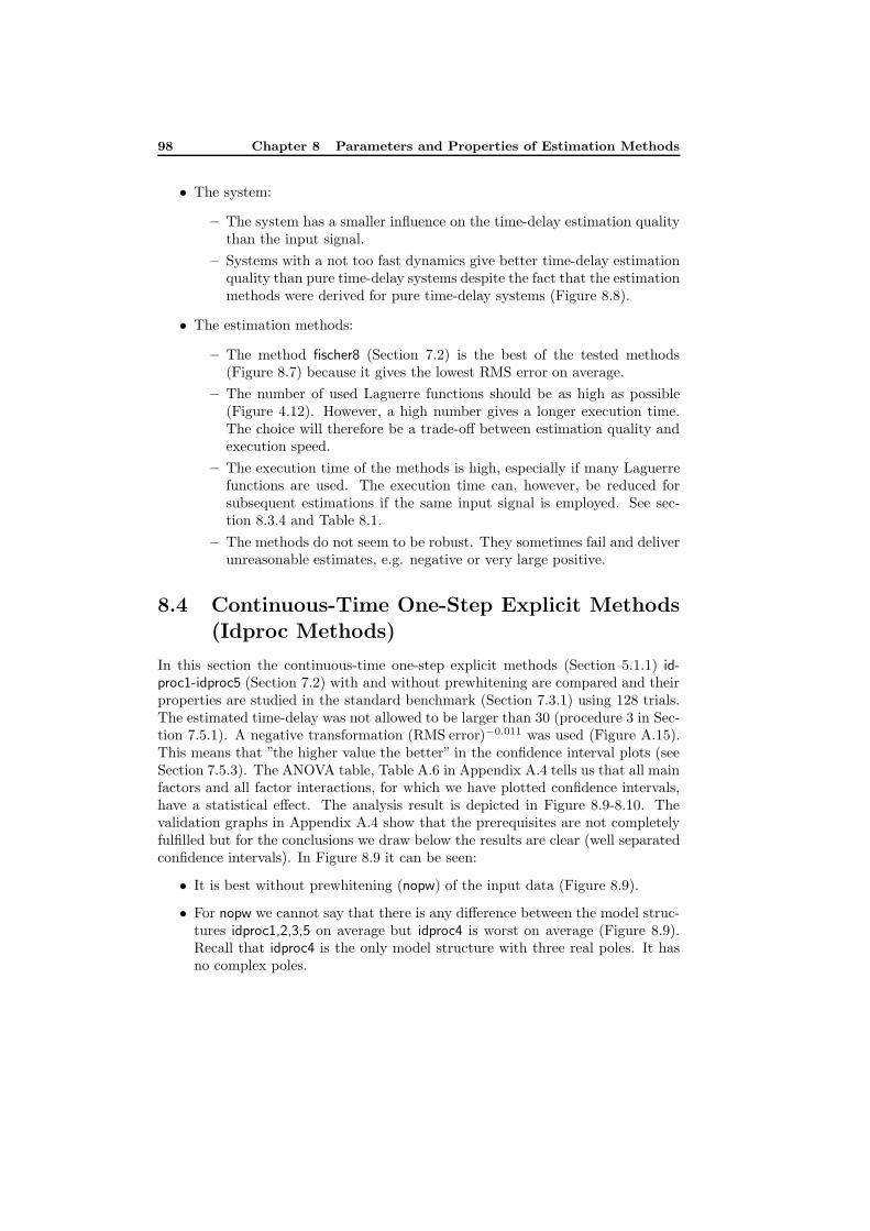
98 Chapter 8 Parameters and Properties of Estimation Methods
• The system:
– The system has a smaller influence on the time-delay estimation qualitythan the input signal.
– Systems with a not too fast dynamics give better time-delay estimationquality than pure time-delay systems despite the fact that the estimationmethods were derived for pure time-delay systems (Figure 8.8).
• The estimation methods:
– The method fischer8 (Section 7.2) is the best of the tested methods(Figure 8.7) because it gives the lowest RMS error on average.
– The number of used Laguerre functions should be as high as possible(Figure 4.12). However, a high number gives a longer execution time.The choice will therefore be a trade-off between estimation quality andexecution speed.
– The execution time of the methods is high, especially if many Laguerrefunctions are used. The execution time can, however, be reduced forsubsequent estimations if the same input signal is employed. See sec-tion 8.3.4 and Table 8.1.
– The methods do not seem to be robust. They sometimes fail and deliverunreasonable estimates, e.g. negative or very large positive.
8.4 Continuous-Time One-Step Explicit Methods(Idproc Methods)
In this section the continuous-time one-step explicit methods (Section 5.1.1) id-proc1-idproc5 (Section 7.2) with and without prewhitening are compared and theirproperties are studied in the standard benchmark (Section 7.3.1) using 128 trials.The estimated time-delay was not allowed to be larger than 30 (procedure 3 in Sec-tion 7.5.1). A negative transformation (RMS error)−0.011 was used (Figure A.15).This means that ”the higher value the better” in the confidence interval plots (seeSection 7.5.3). The ANOVA table, Table A.6 in Appendix A.4 tells us that all mainfactors and all factor interactions, for which we have plotted confidence intervals,have a statistical effect. The analysis result is depicted in Figure 8.9-8.10. Thevalidation graphs in Appendix A.4 show that the prerequisites are not completelyfulfilled but for the conclusions we draw below the results are clear (well separatedconfidence intervals). In Figure 8.9 it can be seen:
• It is best without prewhitening (nopw) of the input data (Figure 8.9).
• For nopw we cannot say that there is any difference between the model struc-tures idproc1,2,3,5 on average but idproc4 is worst on average (Figure 8.9).Recall that idproc4 is the only model structure with three real poles. It hasno complex poles.
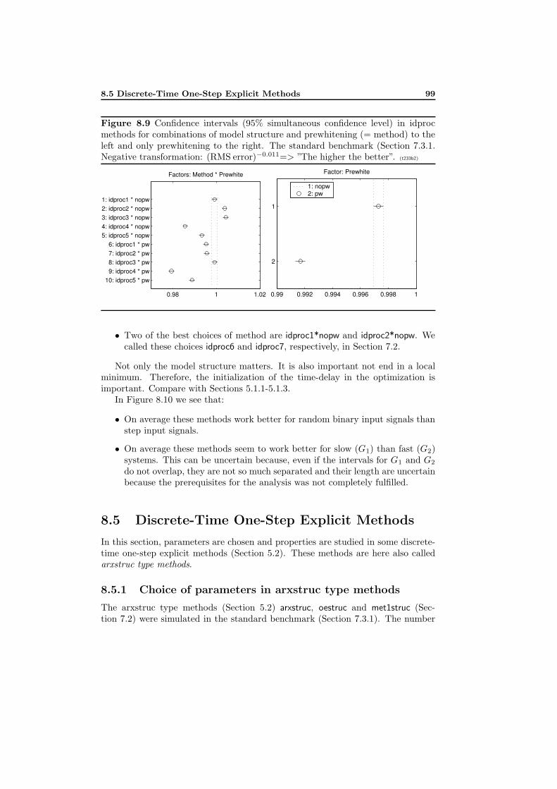
8.5 Discrete-Time One-Step Explicit Methods 99
Figure 8.9 Confidence intervals (95% simultaneous confidence level) in idprocmethods for combinations of model structure and prewhitening (= method) to theleft and only prewhitening to the right. The standard benchmark (Section 7.3.1.Negative transformation: (RMS error)−0.011=> ”The higher the better”. (t233b2)
0.98 1 1.02
10: idproc5 * pw9: idproc4 * pw8: idproc3 * pw7: idproc2 * pw6: idproc1 * pw
5: idproc5 * nopw4: idproc4 * nopw3: idproc3 * nopw2: idproc2 * nopw1: idproc1 * nopw
Factors: Method * Prewhite
PSfrag replacements
tu(t)y(t)s(t)
gts(t)
TdTd
δ(t− Td)g(t)gr(t)g(t)
w(t)r(t)e(t)u(t)y(t)v(t)H(s)F (s)G(s)
0.99 0.992 0.994 0.996 0.998 1
2
1
Factor: Prewhite
1: nopw2: pw
PSfrag replacements
tu(t)y(t)s(t)
gts(t)
TdTd
δ(t− Td)g(t)gr(t)g(t)
w(t)r(t)e(t)u(t)y(t)v(t)H(s)F (s)G(s)
• Two of the best choices of method are idproc1*nopw and idproc2*nopw. Wecalled these choices idproc6 and idproc7, respectively, in Section 7.2.
Not only the model structure matters. It is also important not end in a localminimum. Therefore, the initialization of the time-delay in the optimization isimportant. Compare with Sections 5.1.1-5.1.3.
In Figure 8.10 we see that:
• On average these methods work better for random binary input signals thanstep input signals.
• On average these methods seem to work better for slow (G1) than fast (G2)systems. This can be uncertain because, even if the intervals for G1 and G2
do not overlap, they are not so much separated and their length are uncertainbecause the prerequisites for the analysis was not completely fulfilled.
8.5 Discrete-Time One-Step Explicit Methods
In this section, parameters are chosen and properties are studied in some discrete-time one-step explicit methods (Section 5.2). These methods are here also calledarxstruc type methods.
8.5.1 Choice of parameters in arxstruc type methods
The arxstruc type methods (Section 5.2) arxstruc, oestruc and met1struc (Sec-tion 7.2) were simulated in the standard benchmark (Section 7.3.1). The number
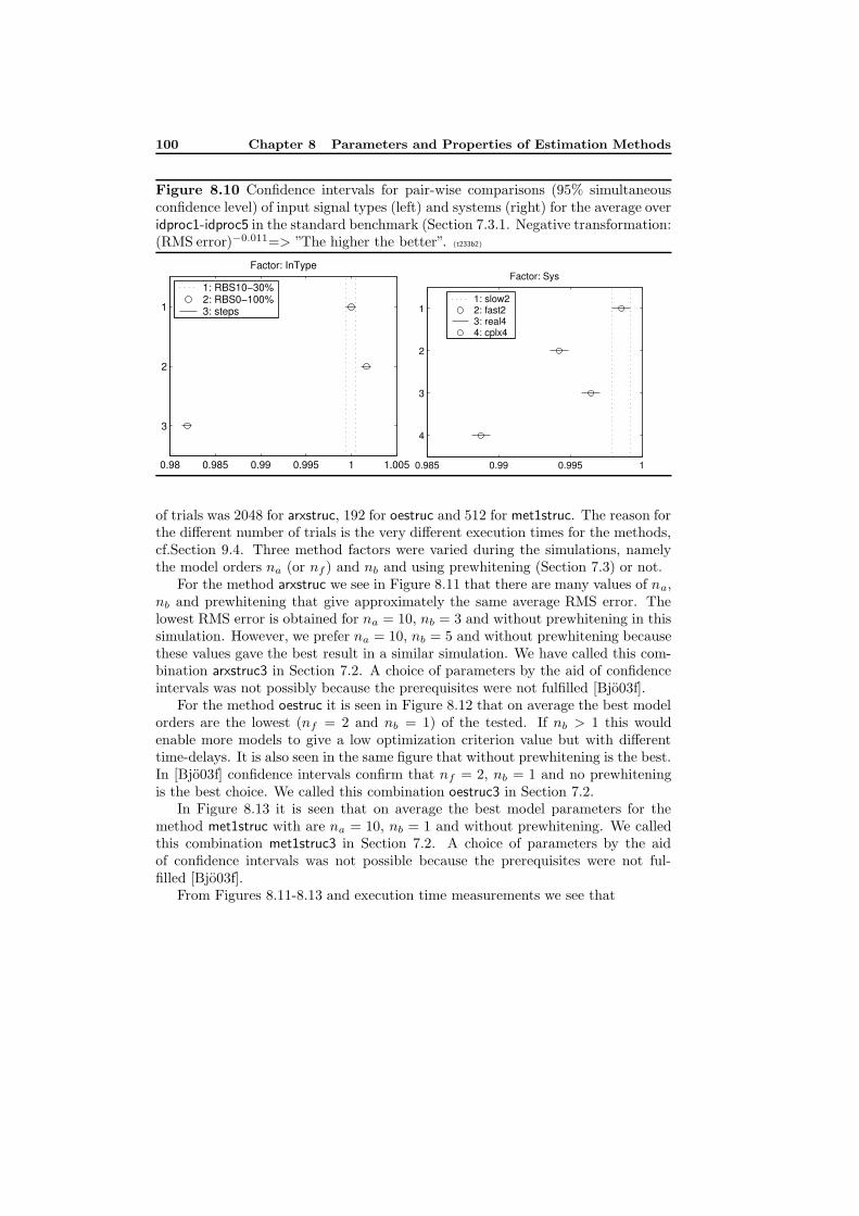
100 Chapter 8 Parameters and Properties of Estimation Methods
Figure 8.10 Confidence intervals for pair-wise comparisons (95% simultaneousconfidence level) of input signal types (left) and systems (right) for the average overidproc1-idproc5 in the standard benchmark (Section 7.3.1. Negative transformation:(RMS error)−0.011=> ”The higher the better”. (t233b2)
0.98 0.985 0.99 0.995 1 1.005
3
2
1
Factor: InType
1: RBS10−30%2: RBS0−100%3: steps
PSfrag replacements
tu(t)y(t)s(t)
gts(t)
TdTd
δ(t− Td)g(t)gr(t)g(t)
w(t)r(t)e(t)u(t)y(t)v(t)H(s)F (s)G(s)
0.985 0.99 0.995 1
4
3
2
1
Factor: Sys
1: slow22: fast23: real44: cplx4
PSfrag replacements
tu(t)y(t)s(t)
gts(t)
TdTd
δ(t− Td)g(t)gr(t)g(t)
w(t)r(t)e(t)u(t)y(t)v(t)H(s)F (s)G(s)
of trials was 2048 for arxstruc, 192 for oestruc and 512 for met1struc. The reason forthe different number of trials is the very different execution times for the methods,cf.Section 9.4. Three method factors were varied during the simulations, namelythe model orders na (or nf ) and nb and using prewhitening (Section 7.3) or not.
For the method arxstruc we see in Figure 8.11 that there are many values of na,nb and prewhitening that give approximately the same average RMS error. Thelowest RMS error is obtained for na = 10, nb = 3 and without prewhitening in thissimulation. However, we prefer na = 10, nb = 5 and without prewhitening becausethese values gave the best result in a similar simulation. We have called this com-bination arxstruc3 in Section 7.2. A choice of parameters by the aid of confidenceintervals was not possibly because the prerequisites were not fulfilled [Bjo03f].
For the method oestruc it is seen in Figure 8.12 that on average the best modelorders are the lowest (nf = 2 and nb = 1) of the tested. If nb > 1 this wouldenable more models to give a low optimization criterion value but with differenttime-delays. It is also seen in the same figure that without prewhitening is the best.In [Bjo03f] confidence intervals confirm that nf = 2, nb = 1 and no prewhiteningis the best choice. We called this combination oestruc3 in Section 7.2.
In Figure 8.13 it is seen that on average the best model parameters for themethod met1struc with are na = 10, nb = 1 and without prewhitening. We calledthis combination met1struc3 in Section 7.2. A choice of parameters by the aidof confidence intervals was not possible because the prerequisites were not ful-filled [Bjo03f].
From Figures 8.11-8.13 and execution time measurements we see that
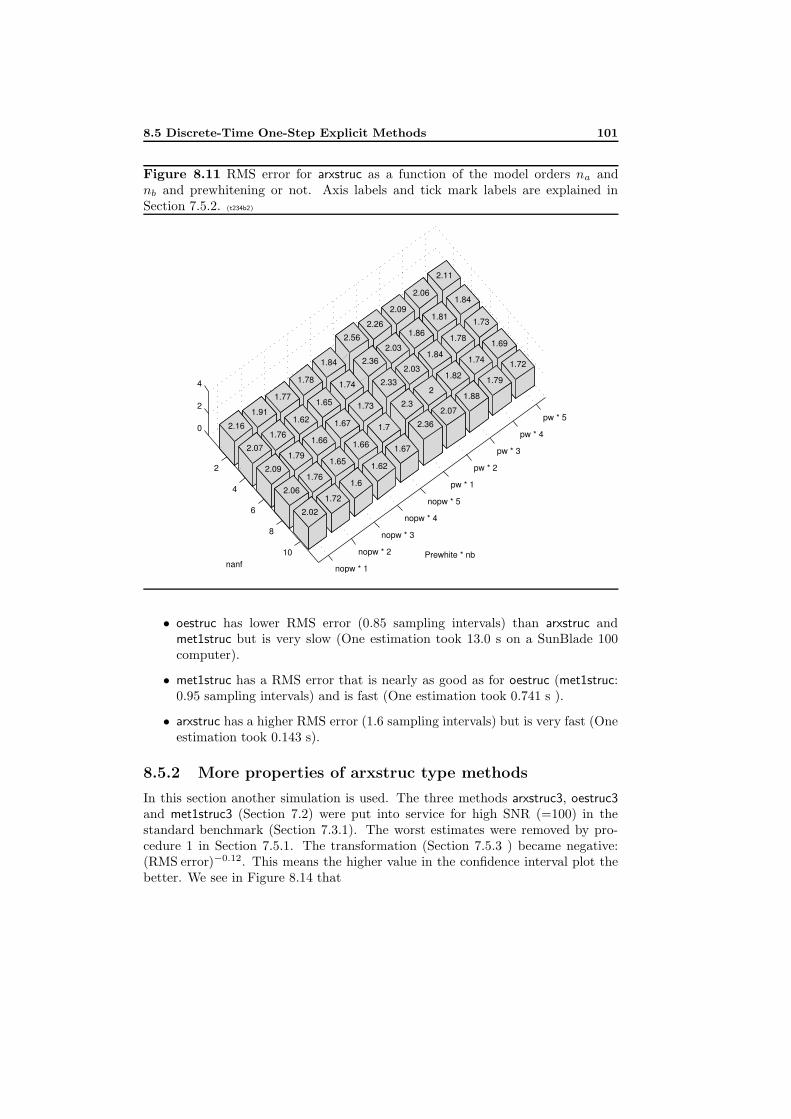
8.5 Discrete-Time One-Step Explicit Methods 101
Figure 8.11 RMS error for arxstruc as a function of the model orders na andnb and prewhitening or not. Axis labels and tick mark labels are explained inSection 7.5.2. (t234b2)
nopw * 1
nopw * 2
nopw * 3
nopw * 4
nopw * 5
pw * 1
pw * 2
pw * 3
pw * 4
pw * 5
2
4
6
8
10
0
2
4
1.72
1.69
1.79
1.73
1.74
1.88
1.84
1.78
1.82
2.07
2.11
1.81
1.84
2
2.36
Prewhite * nb
2.06
1.86
2.03
2.3
1.67
2.09
2.03
2.33
1.7
1.62
2.26
2.36
1.73
1.66
1.6
2.56
1.74
1.67
1.65
1.72
1.84
1.65
1.66
1.76
2.02
1.78
1.62
1.79
2.06
1.77
1.76
2.09
1.91
2.07
nanf
2.16
PSfrag replacements
tu(t)y(t)s(t)
gts(t)
TdTd
δ(t− Td)g(t)gr(t)g(t)
w(t)r(t)e(t)u(t)y(t)v(t)H(s)F (s)G(s)
• oestruc has lower RMS error (0.85 sampling intervals) than arxstruc andmet1struc but is very slow (One estimation took 13.0 s on a SunBlade 100computer).
• met1struc has a RMS error that is nearly as good as for oestruc (met1struc:0.95 sampling intervals) and is fast (One estimation took 0.741 s ).
• arxstruc has a higher RMS error (1.6 sampling intervals) but is very fast (Oneestimation took 0.143 s).
8.5.2 More properties of arxstruc type methods
In this section another simulation is used. The three methods arxstruc3, oestruc3and met1struc3 (Section 7.2) were put into service for high SNR (=100) in thestandard benchmark (Section 7.3.1). The worst estimates were removed by pro-cedure 1 in Section 7.5.1. The transformation (Section 7.5.3 ) became negative:(RMS error)−0.12. This means the higher value in the confidence interval plot thebetter. We see in Figure 8.14 that
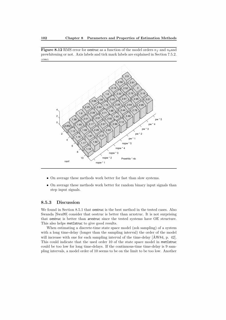
102 Chapter 8 Parameters and Properties of Estimation Methods
Figure 8.12 RMS error for oestruc as a function of the model orders nf and nbandprewhitening or not. Axis labels and tick mark labels are explained in Section 7.5.2.(t236b2)
nopw * 1
nopw * 2
nopw * 3
nopw * 4
nopw * 5
pw * 1
pw * 2
pw * 3
pw * 4
pw * 5
2
4
6
8
10
0
2
4
3.21
3.19
2.95
3
2.95
2.79
2.81
2.79
2.64
2.49
2.9
2.52
2.61
2.44
2.12
Prewhite * nb
2.56
2.32
2.29
1.93
2.99
2.19
2.05
1.88
2.82
2.63
1.8
1.73
2.71
2.57
2.37
1.56
2.62
2.57
2.26
1.92
2.66
2.38
2.17
1.87
1.18
2.25
2.01
1.83
1.17
1.8
1.65
1.19
1.38
1.12
nanf
0.852
PSfrag replacements
tu(t)y(t)s(t)
gts(t)
TdTd
δ(t− Td)g(t)gr(t)g(t)
w(t)r(t)e(t)u(t)y(t)v(t)H(s)F (s)G(s)
• On average these methods work better for fast than slow systems.
• On average these methods work better for random binary input signals thanstep input signals.
8.5.3 Discussion
We found in Section 8.5.1 that oestruc is the best method in the tested cases. AlsoSwanda [Swa99] consider that oestruc is better than arxstruc. It is not surprisingthat oestruc is better than arxstruc since the tested systems have OE structure.This also helps met1struc to give good results.
When estimating a discrete-time state space model (zoh sampling) of a systemwith a long time-delay (longer than the sampling interval) the order of the model
will increase with one for each sampling interval of the time-delay [AW84, p. 42].This could indicate that the used order 10 of the state space model in met1struccould be too low for long time-delays. If the continuous-time time-delay is 9 sam-pling intervals, a model order of 10 seems to be on the limit to be too low. Another
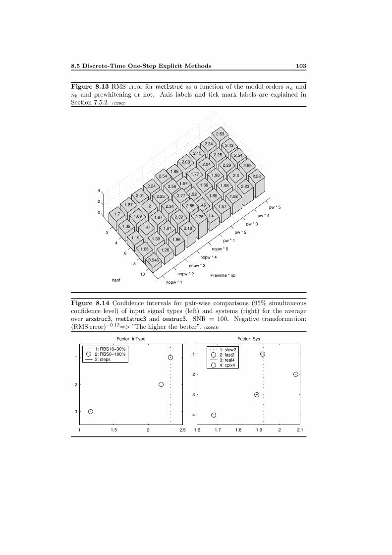
8.5 Discrete-Time One-Step Explicit Methods 103
Figure 8.13 RMS error for met1struc as a function of the model orders na andnb and prewhitening or not. Axis labels and tick mark labels are explained inSection 7.5.2. (t235b2)
nopw * 1
nopw * 2
nopw * 3
nopw * 4
nopw * 5
pw * 1
pw * 2
pw * 3
pw * 4
pw * 5
2
4
6
8
10
0
2
4
2.53
2.59
2.23
2.54
2.3
1.92
2.43
2.29
1.98
1.57
2.63
2.25
1.98
1.65
1.4
Prewhite * nb
2.34
2.04
1.69
1.45
2.75
2.15
1.77
1.52
2.85
2.18
2.08
1.57
2.77
2.32
1.66
1.89
2.56
2.34
1.81
1.26
2.54
2.25
1.87
1.39
0.946
2.24
2
1.51
1.05
2.01
1.69
1.19
1.87
1.39
nanf
1.7
PSfrag replacements
tu(t)y(t)s(t)
gts(t)
TdTd
δ(t− Td)g(t)gr(t)g(t)
w(t)r(t)e(t)u(t)y(t)v(t)H(s)F (s)G(s)
Figure 8.14 Confidence intervals for pair-wise comparisons (95% simultaneousconfidence level) of input signal types (left) and systems (right) for the averageover arxstruc3, met1struc3 and oestruc3. SNR = 100. Negative transformation:(RMS error)−0.12=> ”The higher the better”. (t208b15)
1 1.5 2 2.5
3
2
1
Factor: InType
1: RBS10−30%2: RBS0−100%3: steps
PSfrag replacements
tu(t)y(t)s(t)
gts(t)
TdTd
δ(t− Td)g(t)gr(t)g(t)
w(t)r(t)e(t)u(t)y(t)v(t)H(s)F (s)G(s)
1.6 1.7 1.8 1.9 2 2.1
4
3
2
1
Factor: Sys
1: slow22: fast23: real44: cplx4
PSfrag replacements
tu(t)y(t)s(t)
gts(t)
TdTd
δ(t− Td)g(t)gr(t)g(t)
w(t)r(t)e(t)u(t)y(t)v(t)H(s)F (s)G(s)
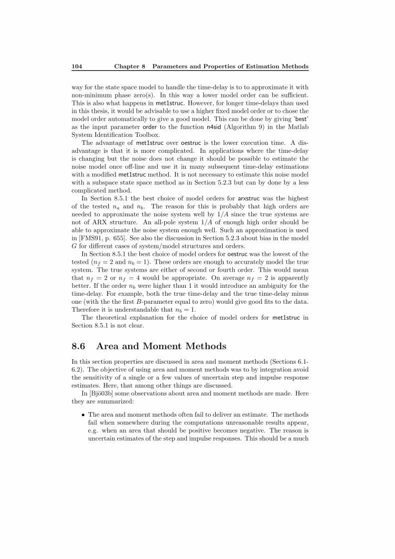
104 Chapter 8 Parameters and Properties of Estimation Methods
way for the state space model to handle the time-delay is to to approximate it withnon-minimum phase zero(s). In this way a lower model order can be sufficient.This is also what happens in met1struc. However, for longer time-delays than usedin this thesis, it would be advisable to use a higher fixed model order or to chose themodel order automatically to give a good model. This can be done by giving ’best’as the input parameter order to the function n4sid (Algorithm 9) in the MatlabSystem Identification Toolbox.
The advantage of met1struc over oestruc is the lower execution time. A dis-advantage is that it is more complicated. In applications where the time-delayis changing but the noise does not change it should be possible to estimate thenoise model once off-line and use it in many subsequent time-delay estimationswith a modified met1struc method. It is not necessary to estimate this noise modelwith a subspace state space method as in Section 5.2.3 but can by done by a lesscomplicated method.
In Section 8.5.1 the best choice of model orders for arxstruc was the highestof the tested na and nb. The reason for this is probably that high orders areneeded to approximate the noise system well by 1/A since the true systems arenot of ARX structure. An all-pole system 1/A of enough high order should beable to approximate the noise system enough well. Such an approximation is usedin [FMS91, p. 655]. See also the discussion in Section 5.2.3 about bias in the modelG for different cases of system/model structures and orders.
In Section 8.5.1 the best choice of model orders for oestruc was the lowest of thetested (nf = 2 and nb = 1). These orders are enough to accurately model the truesystem. The true systems are either of second or fourth order. This would meanthat nf = 2 or nf = 4 would be appropriate. On average nf = 2 is apparentlybetter. If the order nb were higher than 1 it would introduce an ambiguity for thetime-delay. For example, both the true time-delay and the true time-delay minusone (with the the first B-parameter equal to zero) would give good fits to the data.Therefore it is understandable that nb = 1.
The theoretical explanation for the choice of model orders for met1struc inSection 8.5.1 is not clear.
8.6 Area and Moment Methods
In this section properties are discussed in area and moment methods (Sections 6.1-6.2). The objective of using area and moment methods was to by integration avoidthe sensitivity of a single or a few values of uncertain step and impulse responseestimates. Here, that among other things are discussed.
In [Bjo03b] some observations about area and moment methods are made. Herethey are summarized:
• The area and moment methods often fail to deliver an estimate. The methodsfail when somewhere during the computations unreasonable results appear,e.g. when an area that should be positive becomes negative. The reason isuncertain estimates of the step and impulse responses. This should be a much
8.6 Area and Moment Methods 105
smaller problem with measured step and impulse responses as is suggestedin [AH95].
• Moment methods seems to be more unreliable than area methods. Not evenwith a true simulated impulse response they give a good answer. For thesemethods the percentage of failed estimations was very high (>54% for allcombinations of input signals and SNR in the standard benchmark in Sec-tion 7.3.1 but with a different definition of the SNR) in a Monte Carlo simu-lation [Bjo03b]. Therefore these methods are not useful.
• The uncertainty of the step response estimate often increases with the time.Since the gainK, which is used in the area methods, of the system is estimatedby the last step response coefficients this estimate often will be completelyincorrect. This has a very negative effect on the time-delay estimation. Fastsystems seem to have a larger uncertainty in the step response than slowsystems.
• For the area methods (Section 7.2) there are several things that can go wrong:
– The estimated gain K can get negative if the estimated step responsefalls below zero at the end of the estimated step response.
– The estimated area A0 can become negative if too much of the estimatedstep response is above the estimated gain K. This can happen if theestimated gain is too low.
– The time Tar can be estimated to a too high value. This can happen ifthe gain K is estimated to a too low value.
– The time-delay estimate can be calculated to a negative value. Thishappens if either or both Tar is too low and T is too large. The timeconstant T may become too large if the estimated gain K is too low.
• For area and moment methods, the slow low order system (G1) is easier thanthe the fast system (G2). The reason is that the integrals in the area andmoment methods can be better estimated when the function to integrate(impulse or step response ) does not change rapidly. This is the inverse ofthe behavior of many other methods, e.g. thresholding of impulse response,which can easier detect a rapid change than a slow one.
• It is intuitive that fast system is harder for area methods because the A1
integral (Equation 6.4) will be done over a very short time span where thestep response is nonzero.
In [Bjo03b] method parameters were chosen. Below, the terms 1stord and 2ndordmean the first and second order model structures in Section 6.1-6.2. The termstrapez1 and sum1 are two ways to integrate numerically [Bjo03b]. The term nopwmeans without prewhitening the input signal.
• Area methods without prewhitening is better than with prewhitening.
106 Chapter 8 Parameters and Properties of Estimation Methods
• For the area methods there were two combinations of method parameterswhich were better than the other. One of them, the combination nopw*1stord*trapez1, we call area2.
• There is one combination of method parameters for moment methods whichseems to be better than the other: nopw*1stord*sum1. This combination wecall moment2.
Some interesting points are:
• The uncertainty of the estimates of the impulse and step response estimatesare not used in the area and moment methods. If we did not throw away thisinformation we probably could obtain better estimates of the time-delay.
• In the area methods we numerically integrate twice, first from impulse to stepresponse, then to A0 and A1 (Equations 6.3 and 6.4). There will be numericalerrors in both integrations. This could deteriorate the time-delay estimate.But still the area methods are better than the moment methods.
• It is clear that it is important to estimate the gain K (Equations 6.1 and 6.2)correctly in area methods.
• Moment methods are weighting up the later parts of the impulse or stepresponse. This can give large errors because the signal to noise ratio (SNR)is lowered (compare with Section 6.3).
9Comparing Time-Delay EstimationMethods in Open and Closed Loop
In the previous chapter, parameters of time-delay estimation (TDE) methods werechosen. In this chapter, those methods with the chosen parameters are comparedusing Monte Carlo simulations, mainly regarding the estimation quality but alsoregarding the execution time. In Section 9.1 results for open loop simulationswith fixed systems are displayed, in Section 9.2 results for open loop with randomsystems and in 9.3 for closed loop with fixed systems. Execution times are shownin Section 9.4.
9.1 Open Loop Simulations with Fixed Systems
In this section several TDE methods are compared in open loop with fixed systems.
9.1.1 The standard benchmark
This section contains results from comparing several methods in open loop simula-tions with fixed systems (The standard benchmark in Section 7.3.1). The methodsare defined in Section 7.2. See also the list of methods on page 2.
Figure 9.1 shows the average (over all factors) RMS estimation error for severalmethods when the 90%, 95% and 100% best estimates are retained (procedure 1in Section 7.5.1). The methods oestruc3 and met1struc3 are the best methodswhen 100% are used. For 90%-95%, they are challenged by idproc7. The methodsoestruc3 and met1struc3 are better than arxstruc3. The method idproc7 is betterthan idproc6. The method idproc7 mostly gives very accurate estimates but some-times fails. It is favored by only retaining the 90%-95% best estimates. The method
107
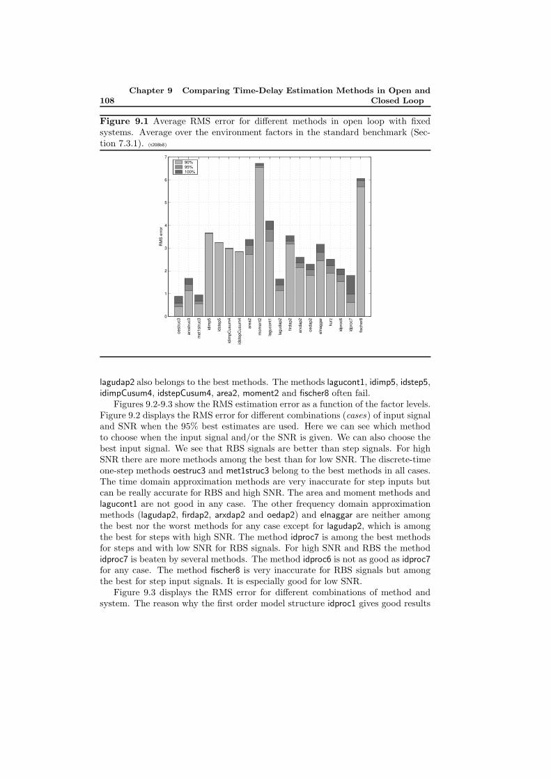
108Chapter 9 Comparing Time-Delay Estimation Methods in Open and
Closed Loop
Figure 9.1 Average RMS error for different methods in open loop with fixedsystems. Average over the environment factors in the standard benchmark (Sec-tion 7.3.1). (t208b8)
0
1
2
3
4
5
6
7
oest
ruc3
arxs
truc3
met
1stru
c3
idim
p5
idst
ep5
idim
pCus
um4
idst
epC
usum
4
area
2
mom
ent2
lagu
cont
1
lagu
dap2
firda
p2
arxd
ap2
oeda
p2
elna
ggar
kurz
idpr
oc6
idpr
oc7
fisch
er8
RM
S e
rror
90% 95% 100%
PSfrag replacements
tu(t)y(t)s(t)
gts(t)
TdTd
δ(t− Td)g(t)gr(t)g(t)
w(t)r(t)e(t)u(t)y(t)v(t)H(s)F (s)G(s)
lagudap2 also belongs to the best methods. The methods lagucont1, idimp5, idstep5,idimpCusum4, idstepCusum4, area2, moment2 and fischer8 often fail.
Figures 9.2-9.3 show the RMS estimation error as a function of the factor levels.Figure 9.2 displays the RMS error for different combinations (cases) of input signaland SNR when the 95% best estimates are used. Here we can see which methodto choose when the input signal and/or the SNR is given. We can also choose thebest input signal. We see that RBS signals are better than step signals. For highSNR there are more methods among the best than for low SNR. The discrete-timeone-step methods oestruc3 and met1struc3 belong to the best methods in all cases.The time domain approximation methods are very inaccurate for step inputs butcan be really accurate for RBS and high SNR. The area and moment methods andlagucont1 are not good in any case. The other frequency domain approximationmethods (lagudap2, firdap2, arxdap2 and oedap2) and elnaggar are neither amongthe best nor the worst methods for any case except for lagudap2, which is amongthe best for steps with high SNR. The method idproc7 is among the best methodsfor steps and with low SNR for RBS signals. For high SNR and RBS the methodidproc7 is beaten by several methods. The method idproc6 is not as good as idproc7for any case. The method fischer8 is very inaccurate for RBS signals but amongthe best for step input signals. It is especially good for low SNR.
Figure 9.3 displays the RMS error for different combinations of method andsystem. The reason why the first order model structure idproc1 gives good results
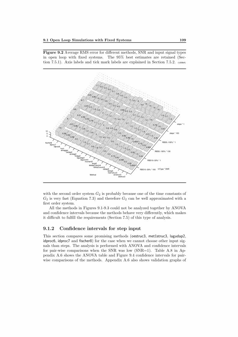
9.1 Open Loop Simulations with Fixed Systems 109
Figure 9.2 Average RMS error for different methods, SNR and input signal typesin open loop with fixed systems. The 95% best estimates are retained (Sec-tion 7.5.1). Axis labels and tick mark labels are explained in Section 7.5.2. (t208b9)
RBS10−30% * 100
RBS10−30% * 1
RBS0−100% * 100
RBS0−100% * 1
steps * 100
steps * 1
oestruc3arxstruc3
met1struc3idimp5
idstep5idimpCusum4
idstepCusum4area2
moment2lagucont1
lagudap2firdap2
arxdap2oedap2
elnaggarkurz
idproc6idproc7
fischer8
05
10
1.93.7
0.67
1.9
1.8
10
InType * SNR
0.45
0.79
10
1.2
7.6
10
0.063
0.57
3.1
10
0.31
1.9
5.1
4.4
0.44
0.15
2.1
3.1
8
1.2
0.00011
1.2
2.1
5.3
0.00011
0.52
1.9
1.5
5.3
3
0.29
2.3
0.38
3.7
2.4
4.3
0.2
1.4
0.56
7.6
0.92
4.2
0.048
1.1
2.2
4.4
4.3
3.8
0.91
1.5
5.6
1.5
2.2
5.1
0.13
3.9
4.5
3.1
2.3
5.2
0.3
7.5
0.8
1.7
3.8
4.3
2.5
4.5
3
2
3.3
3.2
5.7
1.4
1.7
3.9
1.9
1.7
1.8
3
Method
1.1
1.8
0.89
0.6
2.9
0.76
2.3
0.81
2.1
2.1
0.53
0.57
1.6
2.8
0.59
8.7
1
2
0.31
0.5
0.99
8.8
0.58
0.57
0.92
8
0.29
7.9
PSfrag replacements
tu(t)y(t)s(t)
gts(t)
TdTd
δ(t− Td)g(t)gr(t)g(t)
w(t)r(t)e(t)u(t)y(t)v(t)H(s)F (s)G(s)
with the second order system G2 is probably because one of the time constants ofG2 is very fast (Equation 7.3) and therefore G2 can be well approximated with afirst order system.
All the methods in Figures 9.1-9.3 could not be analyzed together by ANOVAand confidence intervals because the methods behave very differently, which makesit difficult to fulfill the requirements (Section 7.5) of this type of analysis.
9.1.2 Confidence intervals for step input
This section compares some promising methods (oestruc3, met1struc3, lagudap2,idproc6, idproc7 and fischer8) for the case when we cannot choose other input sig-nals than steps. The analysis is performed with ANOVA and confidence intervalsfor pair-wise comparisons when the SNR was low (SNR=1). Table A.8 in Ap-pendix A.6 shows the ANOVA table and Figure 9.4 confidence intervals for pair-wise comparisons of the methods. Appendix A.6 also shows validation graphs of
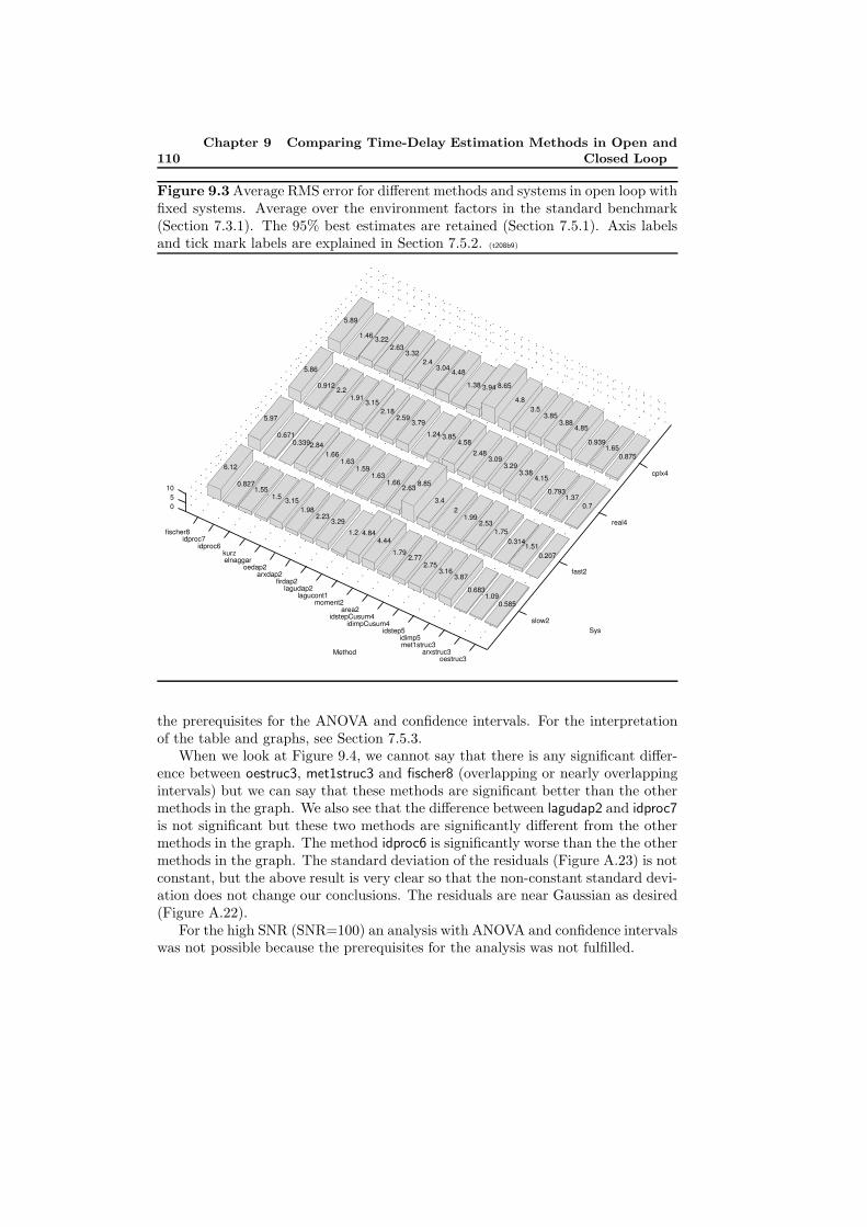
110Chapter 9 Comparing Time-Delay Estimation Methods in Open and
Closed Loop
Figure 9.3 Average RMS error for different methods and systems in open loop withfixed systems. Average over the environment factors in the standard benchmark(Section 7.3.1). The 95% best estimates are retained (Section 7.5.1). Axis labelsand tick mark labels are explained in Section 7.5.2. (t208b9)
slow2
fast2
real4
cplx4
oestruc3arxstruc3
met1struc3idimp5
idstep5idimpCusum4
idstepCusum4area2
moment2lagucont1
lagudap2firdap2
arxdap2oedap2
elnaggarkurz
idproc6idproc7
fischer8
05
10
0.8751.65
0.939
Sys
0.7
4.85
1.37
3.88
0.793
3.85
0.207
4.15
3.5
1.51
3.38
4.8
0.314
3.29
0.585
8.65
1.75
3.09
1.09
3.94
2.53
2.48
0.683
1.38
1.99
4.58
3.87
4.48
2
3.85
3.16
3.04
3.4
1.24
2.75
2.4
8.85
3.79
2.77
3.32
2.63
2.59
1.79
2.63
1.66
2.18
4.44
3.22
1.63
3.15
4.84
1.46
1.59
1.91
Method
1.2
5.89
1.63
2.2
3.29
1.66
0.912
2.23
2.84
5.86
1.98
0.339
3.15
0.671
1.5
5.97
1.550.827
6.12
PSfrag replacements
tu(t)y(t)s(t)
gts(t)
TdTd
δ(t− Td)g(t)gr(t)g(t)
w(t)r(t)e(t)u(t)y(t)v(t)H(s)F (s)G(s)
the prerequisites for the ANOVA and confidence intervals. For the interpretationof the table and graphs, see Section 7.5.3.
When we look at Figure 9.4, we cannot say that there is any significant differ-ence between oestruc3, met1struc3 and fischer8 (overlapping or nearly overlappingintervals) but we can say that these methods are significant better than the othermethods in the graph. We also see that the difference between lagudap2 and idproc7is not significant but these two methods are significantly different from the othermethods in the graph. The method idproc6 is significantly worse than the the othermethods in the graph. The standard deviation of the residuals (Figure A.23) is notconstant, but the above result is very clear so that the non-constant standard devi-ation does not change our conclusions. The residuals are near Gaussian as desired(Figure A.22).
For the high SNR (SNR=100) an analysis with ANOVA and confidence intervalswas not possible because the prerequisites for the analysis was not fulfilled.
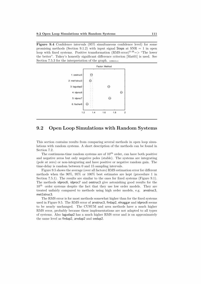
9.2 Open Loop Simulations with Random Systems 111
Figure 9.4 Confidence intervals (95% simultaneous confidence level) for somepromising methods (Section 9.1.2) with input signal Steps at SNR = 1 in openloop with fixed systems. Positive transformation (RMS error)0.48=> “The lowerthe better”. Tukey’s honestly significant difference criterion [Mat01] is used. SeeSection 7.5.3 for the interpretation of the graph. (t208b10.m)
1.2 1.4 1.6 1.8 2
6: fischer8
5: idproc7
4: idproc6
3: lagudap2
2: met1struc3
1: oestruc3
Factor: Method
PSfrag replacements
tu(t)y(t)s(t)
gts(t)
TdTd
δ(t− Td)g(t)gr(t)g(t)
w(t)r(t)e(t)u(t)y(t)v(t)H(s)F (s)G(s)
9.2 Open Loop Simulations with Random Systems
This section contains results from comparing several methods in open loop simu-lations with random systems. A short description of the methods can be found inSection 7.2.
The continuous-time random systems are of 10th order, can have both positiveand negative zeros but only negative poles (stable). The systems are integrating(pole at zero) or non-integrating and have positive or negative random gain. Thetime-delay is random between 0 and 15 sampling intervals.
Figure 9.5 shows the average (over all factors) RMS estimation error for differentmethods when the 90%, 95% or 100% best estimates are kept (procedure 1 inSection 7.5.1). The results are similar to the ones for fixed systems (Figure 9.1).The methods idproc6, idproc7 and oestruc3 give astonishing good results for the10th order systems despite the fact that they use low order models. They aretreated unfairly compared to methods using high order models, e.g. arxstruc3,met1struc3.
The RMS error is for most methods somewhat higher than for the fixed systemsused in Figure 9.5. The RMS error of arxstruc3, firdap2, elnaggar and idproc6 seemsto be nearly unchanged. The CUSUM and area methods have a much higherRMS error, probably because these implementations are not adapted to all typesof systems. Also lagudap2 has a much higher RMS error and is on approximatelythe same level as firdap2, arxdap2 and oedap2.
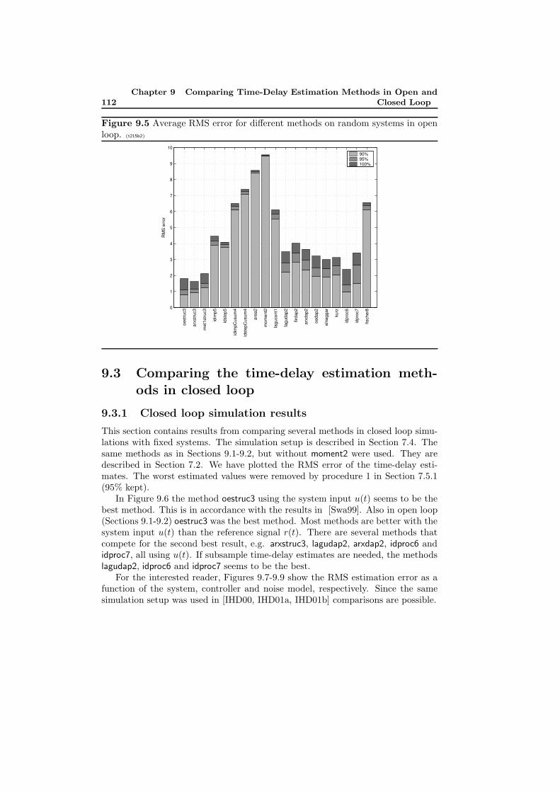
112Chapter 9 Comparing Time-Delay Estimation Methods in Open and
Closed Loop
Figure 9.5 Average RMS error for different methods on random systems in openloop. (t215b2)
0
1
2
3
4
5
6
7
8
9
10
oest
ruc3
arxs
truc3
met
1stru
c3
idim
p5
idst
ep5
idim
pCus
um4
idst
epC
usum
4
area
2
mom
ent2
lagu
cont
1
lagu
dap2
firda
p2
arxd
ap2
oeda
p2
elna
ggar
kurz
idpr
oc6
idpr
oc7
fisch
er8
RM
S e
rror
90% 95% 100%
PSfrag replacements
tu(t)y(t)s(t)
gts(t)
TdTd
δ(t− Td)g(t)gr(t)g(t)
w(t)r(t)e(t)u(t)y(t)v(t)H(s)F (s)G(s)
9.3 Comparing the time-delay estimation meth-
ods in closed loop
9.3.1 Closed loop simulation results
This section contains results from comparing several methods in closed loop simu-lations with fixed systems. The simulation setup is described in Section 7.4. Thesame methods as in Sections 9.1-9.2, but without moment2 were used. They aredescribed in Section 7.2. We have plotted the RMS error of the time-delay esti-mates. The worst estimated values were removed by procedure 1 in Section 7.5.1(95% kept).
In Figure 9.6 the method oestruc3 using the system input u(t) seems to be thebest method. This is in accordance with the results in [Swa99]. Also in open loop(Sections 9.1-9.2) oestruc3 was the best method. Most methods are better with thesystem input u(t) than the reference signal r(t). There are several methods thatcompete for the second best result, e.g. arxstruc3, lagudap2, arxdap2, idproc6 andidproc7, all using u(t). If subsample time-delay estimates are needed, the methodslagudap2, idproc6 and idproc7 seems to be the best.
For the interested reader, Figures 9.7-9.9 show the RMS estimation error as afunction of the system, controller and noise model, respectively. Since the samesimulation setup was used in [IHD00, IHD01a, IHD01b] comparisons are possible.
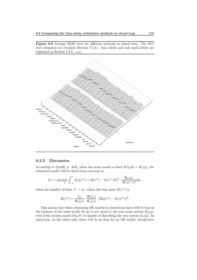
9.3 Comparing the time-delay estimation methods in closed loop 113
Figure 9.6 Average RMS error for different methods in closed loop. The 95%best estimates are retained (Section 7.5.1). Axis labels and tick mark labels areexplained in Section 7.5.2. (t176d2)
u
r
oestruc3arxstruc3
met1struc3idimp5
idstep5idimpCusum4
idstepCusum4area2lagudap2
firdap2arxdap2
oedap2elnaggar
kurzidproc6
idproc7fischer8
6.332.38
2.25
InputPlace
7.833.21
6.162.81
8.38
5.73
5.67
2.08
6.26
3.56
5.23
3.86
4.27
9.97
3.3
7.68
3.74
9.84
5.03
3.19
2.78
2.63
5.56
0.73
8.36
Method
7.516.89
9.265.6
2.773.2
PSfrag replacements
tu(t)y(t)s(t)
gts(t)
TdTd
δ(t− Td)g(t)gr(t)g(t)
w(t)r(t)e(t)u(t)y(t)v(t)H(s)F (s)G(s)
9.3.2 Discussion
According to [Lju99, p. 433], when the noise model is fixed H(q, θ) = H∗(q), theestimated model will in closed loop converge to
G∗ = arg minθ
∫ π
−π|G0(eiω) +B(eiω)−G(eiω , θ)|2 · Φu(ω)
|H∗(eiω)|2 dω,
when the number of data N →∞, where the bias term B(eiω) is
B(eiω) =λ0
Φu(ω)· Φeu(ω)
Φu(ω)· |H0(eiω)−H∗(eiω)|2.
This means that when estimating OE models in closed loop there will be bias inthe estimate if the noise model H∗(q) is not equal to the true noise system H0(q),even if the system model G(q, θ) is capable of describing the true system G0(q). Inopen-loop, on the other side, there will be no bias for an OE model, irrespective
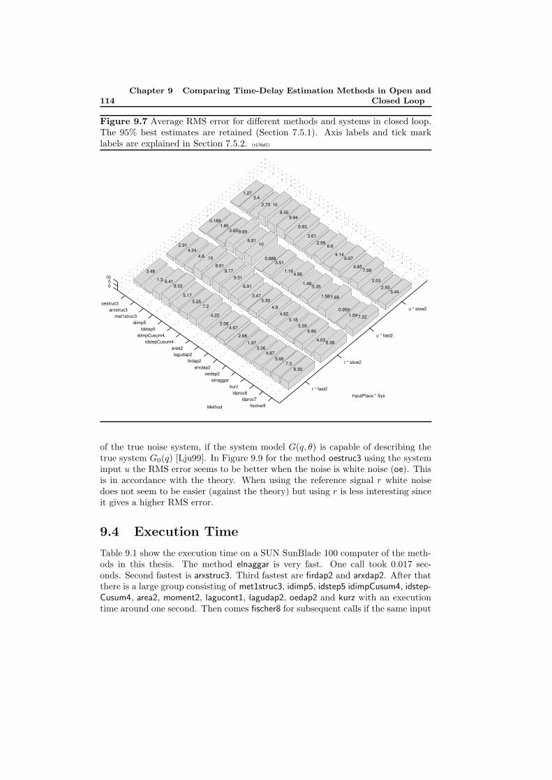
114Chapter 9 Comparing Time-Delay Estimation Methods in Open and
Closed Loop
Figure 9.7 Average RMS error for different methods and systems in closed loop.The 95% best estimates are retained (Section 7.5.1). Axis labels and tick marklabels are explained in Section 7.5.2. (t176d2)
u * slow2
u * fast2
r * slow2
r * fast2
oestruc3arxstruc3
met1struc3idimp5
idstep5idimpCusum4
idstepCusum4area2lagudap2
firdap2arxdap2
oedap2elnaggar
kurzidproc6
idproc7fischer8
05
10
5.442.93
3.53
7.98
7.22
4.85
1.84
InputPlace * Sys
6.97
0.959
4.14
7.68
6.6
8.38
1.56
2.99
4.03
5.35
3.61
6.86
1.48
6.83
5.59
4.86
8.39
9.94
5.18
1.16
7.3
8.55
4.62
3.51
5.66
10
4.8
0.888
4.87
2.73
5.39
10
3.36
3.4
3.47
6.81
1.97
1.27
6.91
9.69
2.68
9.51
3.65
4.67
9.77
1.85
2.08
Method
8.61
0.189
4.22
10
7.2
4.8
5.25
4.24
5.17
2.91
8.536.411.3
3.48
PSfrag replacements
tu(t)y(t)s(t)
gts(t)
TdTd
δ(t− Td)g(t)gr(t)g(t)
w(t)r(t)e(t)u(t)y(t)v(t)H(s)F (s)G(s)
of the true noise system, if the system model G(q, θ) is capable of describing thetrue system G0(q) [Lju99]. In Figure 9.9 for the method oestruc3 using the systeminput u the RMS error seems to be better when the noise is white noise (oe). Thisis in accordance with the theory. When using the reference signal r white noisedoes not seem to be easier (against the theory) but using r is less interesting sinceit gives a higher RMS error.
9.4 Execution Time
Table 9.1 show the execution time on a SUN SunBlade 100 computer of the meth-ods in this thesis. The method elnaggar is very fast. One call took 0.017 sec-onds. Second fastest is arxstruc3. Third fastest are firdap2 and arxdap2. After thatthere is a large group consisting of met1struc3, idimp5, idstep5 idimpCusum4, idstep-Cusum4, area2, moment2, lagucont1, lagudap2, oedap2 and kurz with an executiontime around one second. Then comes fischer8 for subsequent calls if the same input
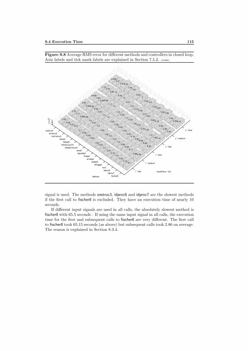
9.4 Execution Time 115
Figure 9.8 Average RMS error for different methods and controllers in closed loop.Axis labels and tick mark labels are explained in Section 7.5.2. (t176d2)
u * slow
u * medium
u * fast
r * slow
r * medium
r * fast
oestruc3arxstruc3
met1struc3idimp5
idstep5idimpCusum4
idstepCusum4area2lagudap2
firdap2arxdap2
oedap2elnaggar
kurzidproc6
idproc7fischer8
05
108.152.32
1.94
3.43
7.85
2.98
3.05
3.59
7.41
6.25
8.18
InputPlace * Ctrl
1.85
2.42
3.82
1.21
6.5
8.36
6.81
7.45
2.32
8.98
4.47
2.76
5
8.08
6.35
8.39
5.42
3.59
4.96
2.74
2.86
1.52
9.9
4.19
3.31
6.17
4.33
7.44
8.4
3.33
6.07
5.84
1.17
9.53
5.16
4.45
10
4.89
2.36
3.47
4.52
6.46
8.42
3.9
1.91
2.47
4.9
5.58
10
4.07
10
0.646
3.72
5.92
3.83
5.2
7.17
2.67
10
3.76
1.66
9.99
2.7
7.9
1.12
4.83
2.29
3.44
9.07
Method
9.5
1.66
1.09
9.59
9.57
0.429
5.94
8.85
7.9
5.58
2.52
9.99
5.06
3.49
3.69
3.7
3.71
8.21
2.75
4.272.08
3.35
PSfrag replacements
tu(t)y(t)s(t)
gts(t)
TdTd
δ(t− Td)g(t)gr(t)g(t)
w(t)r(t)e(t)u(t)y(t)v(t)H(s)F (s)G(s)
signal is used. The methods oestruc3, idproc6 and idproc7 are the slowest methodsif the first call to fischer8 is excluded. They have an execution time of nearly 10seconds.
If different input signals are used in all calls, the absolutely slowest method isfischer8 with 65.5 seconds . If using the same input signal in all calls, the executiontime for the first and subsequent calls to fischer8 are very different. The first callto fischer8 took 65.15 seconds (as above) but subsequent calls took 2.86 on average.The reason is explained in Section 8.3.4.
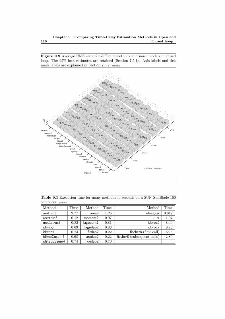
116Chapter 9 Comparing Time-Delay Estimation Methods in Open and
Closed Loop
Figure 9.9 Average RMS error for different methods and noise models in closedloop. The 95% best estimates are retained (Section 7.5.1). Axis labels and tickmark labels are explained in Section 7.5.2. (t176d2)
u * filt
u * oe
u * arx
r * filt
r * oe
r * arx
oestruc3arxstruc3
met1struc3idimp5
idstep5idimpCusum4
idstepCusum4area2lagudap2
firdap2arxdap2
oedap2elnaggar
kurzidproc6
idproc7fischer8
05
10
6.292.3
1.5
6.37
7.37
2.63
2.97
3.04
6.33
8.94
7.92
InputPlace * NoiseMod
2.22
3.02
3.56
2.2
8.26
8.38
2.17
8.19
3.59
5.79
2.8
3.1
5.76
6.13
2.67
8.38
7.37
4.46
5.39
1.24
5.65
2.6
9.9
3.86
1.87
6.39
6.26
10
8.38
3.62
3.54
5.17
1.39
9.52
5.56
3.9
10
4.6
3.04
4.21
6.26
5.09
3.04
3
3.58
2.37
5.13
2.82
10
3.51
10
0.868
4.34
5.72
2.25
4.98
10
3.28
8.62
2.49
2.71
10
3.81
6.55
0.608
5.48
3.13
5.03
5.63
Method
8.14
3.02
2.79
8.51
8.27
0.714
5.49
6.09
7.93
8.32
2.81
9.79
7.71
3.18
5.07
7.11
2.76
9.49
3.21
5.642.74
3.2
PSfrag replacements
tu(t)y(t)s(t)
gts(t)
TdTd
δ(t− Td)g(t)gr(t)g(t)
w(t)r(t)e(t)u(t)y(t)v(t)H(s)F (s)G(s)
Table 9.1 Execution time for many methods in seconds on a SUN SunBlade 100computer. (t227b1)
Method Time Method Time Method Time
oestruc3 9.77 area2 1.26 elnaggar 0.017arxstruc3 0.12 moment2 0.97 kurz 1.07met1struc3 0.82 lagucont1 0.81 idproc6 8.40idimp5 0.69 lagudap2 0.83 idproc7 9.76idstep5 0.74 firdap2 0.22 fischer8 (first call) 65.5idimpCusum4 0.68 arxdap2 0.22 fischer8 (subsequent calls) 2.86idstepCusum4 0.74 oedap2 0.70
10Discussion and Conclusions
This chapter contains further discussion in Section 10.1. Then, in Section 10.2,recommendations for the choice of time-delay estimation (TDE) method for differ-ent cases are given. Following, Section 10.3 contains conclusions about propertiesof different classes (Chapter 3) of TDE methods. Finally, in Section 10.4 somesuggestions for future work are listed.
10.1 Additional Discussion about Open Loop
In this section we will give some additional discussion about open-loop. The TDEmethods are described in Section 7.2.
The methods idimp5, idstep5, idimpCusum4 and idstepCusum4 often miss todetect the start of the impulse response (Sections 4.1.1 and 4.1.3), especially for lowSNR, because of noisy and uncertain impulse and step response estimates [Bjo03d].Prewhitening of step input does not make idimp4 perform better (Section 8.1.1).Prewhitening can make the cross-correlation contain fewer maxima that competewith the correct one [Car93]. Maybe prewhitening amplifies the noise in certainfrequency regions and thereby counteracts the increase in estimation performance.
The method lagudap2 performs well in most cases (but not best) and seldomreally bad. Two reasons for lagudap2 being better than firdap2, arxdap2 and oedap2are probably that typical impulse responses can be described well by Laguerrefunctions and that the model orders of the latter methods are not optimal. Themodel orders of the DAP methods should also have been selected via Monte Carlosimulations, which was not done in this thesis (except for the zero guarding). Theresults in [Hor00] for lagudap2 is in agreement with our results. lagucont1 often fails,
117
118 Chapter 10 Discussion and Conclusions
probably because it has no protection against noise-corrupted zeros. The resultsin [Hor00] for lagucont1 is better than our results. Perhaps, the implementationin [Hor00] has some protection against bad zeros.
idproc7 is better than idproc6 as it has a more suitable model structure for theused systems. Both these model structures have a too low order for some of thetested systems. Therefore they will have some bias. Since oestruc3 and met1struc3have the correct model structure (output error) they are better than arxstruc3.
area2 and moment2 often give very inaccurate estimates due to poor estimatesof step and impulse responses [Bjo03b, Ing03]. These methods would probably
perform better with measured step and impulse responses as in [AH95]. Anotherimprovement is described in [Ing03].
The method fischer8 often give very poor estimates. This is probably due toits inability to describe certain signals in the Laguerre domain [Bjo03e]. On theother hand, fischer8 performs astonishingly well for steps, especially at low SNR.Perhaps it would be even better with more Laguerre coefficients. The used number,150, was on the limit of being too computer intensive.
Some of the tested methods can estimate subsample time-delays. In, for exam-ple, time-delay of arrival estimation of the direction of impinging electro-magneticwaves in signal intelligence [HR97, FHJ02] or radar this is necessary.
10.2 Recommendations for Choice of EstimationMethod
This section gives recommendations on which TDE method to choose in differentcases. The methods are described in Section 7.2.
In open loop the method oestruc3 is best on average with respect to estimationquality (Sections 9.1-9.2). If sub-sample time-delay estimates are needed, the bestmethod (Section 9.1) is idproc7 but keep in mind that the model structure shouldbe the same as the true system. On the negative side, both oestruc3 and idproc7have long execution times, which could be a limiting factor in some applications.There are other, much faster, methods, e.g. met1struc3, arxstruc3 and lagudap2,with nearly as good estimation quality.
Some of the tested methods can deliver estimates of subsample time-delays.These are the frequency domain methods, e.g. lagudap2, and the continuous-timeone-step explicit methods, e.g. idproc6 and idproc7.
Recommendations for the choice of input signal and estimation method in openloop for the best estimation quality are:
• If you cannot use other input signals than steps: For high SNR use oestruc3,met1struc3, lagudap2, idproc7 or fischer8. If the SNR is low use only oestruc3,met1struc3 or fischer8. If subsample time-delay estimates are needed for lowSNR use lagudap2 or idproc7 (Figures 9.2 and 9.4).
• If you can choose the input signal, use RBS (Random Binary) signals. Forhigh SNR the best methods are oestruc3 and idimp5. There are, however,more methods giving good results. If subsample time-delay estimates are
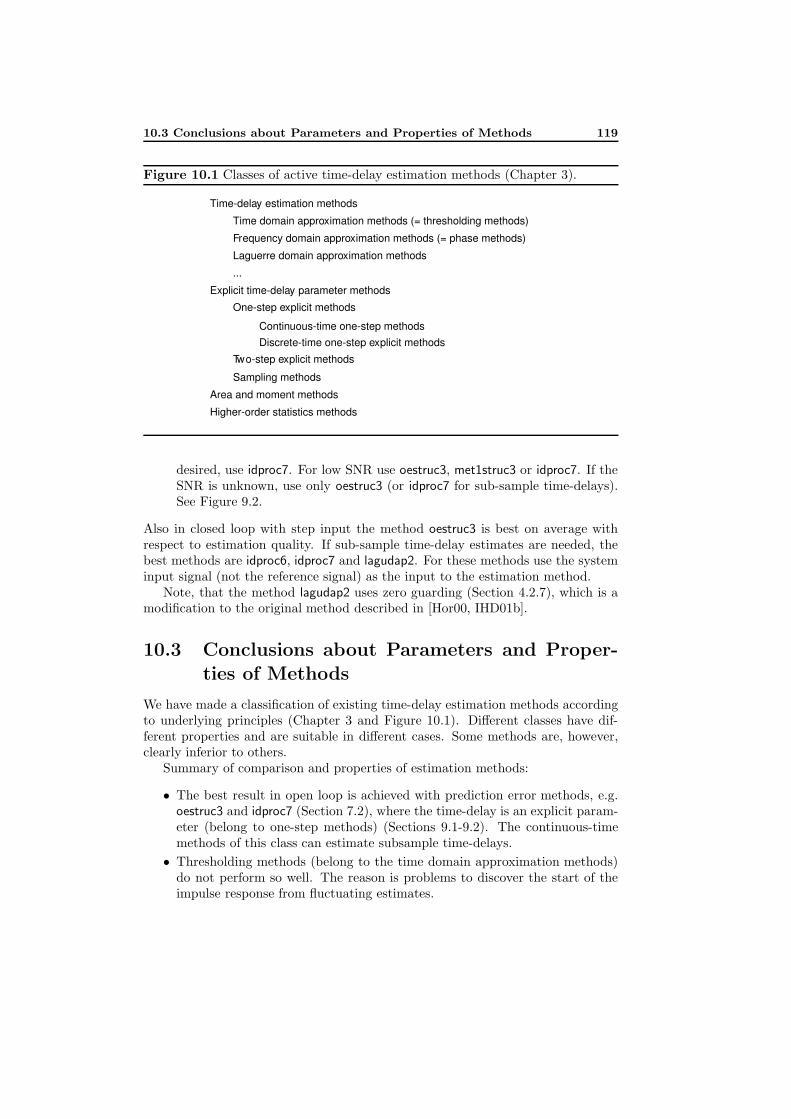
10.3 Conclusions about Parameters and Properties of Methods 119
Figure 10.1 Classes of active time-delay estimation methods (Chapter 3).
Time-delay estimation methods
Time domain approximation methods (= thresholding methods)
Frequency domain approximation methods (= phase methods)
Laguerre domain approximation methods
Explicit time-delay parameter methods
Discrete-time one-step explicit methods
Sampling methods
Area and moment methods
Higher-order statistics methods
...
One-step explicit methods
Continuous-time one-step methods
Two-step explicit methods
PSfrag replacements
tu(t)y(t)s(t)
gts(t)
TdTd
δ(t− Td)g(t)gr(t)g(t)
w(t)r(t)e(t)u(t)y(t)v(t)H(s)F (s)G(s)
desired, use idproc7. For low SNR use oestruc3, met1struc3 or idproc7. If theSNR is unknown, use only oestruc3 (or idproc7 for sub-sample time-delays).See Figure 9.2.
Also in closed loop with step input the method oestruc3 is best on average withrespect to estimation quality. If sub-sample time-delay estimates are needed, thebest methods are idproc6, idproc7 and lagudap2. For these methods use the systeminput signal (not the reference signal) as the input to the estimation method.
Note, that the method lagudap2 uses zero guarding (Section 4.2.7), which is amodification to the original method described in [Hor00, IHD01b].
10.3 Conclusions about Parameters and Proper-
ties of Methods
We have made a classification of existing time-delay estimation methods accordingto underlying principles (Chapter 3 and Figure 10.1). Different classes have dif-ferent properties and are suitable in different cases. Some methods are, however,clearly inferior to others.
Summary of comparison and properties of estimation methods:
• The best result in open loop is achieved with prediction error methods, e.g.oestruc3 and idproc7 (Section 7.2), where the time-delay is an explicit param-eter (belong to one-step methods) (Sections 9.1-9.2). The continuous-timemethods of this class can estimate subsample time-delays.
• Thresholding methods (belong to the time domain approximation methods)do not perform so well. The reason is problems to discover the start of theimpulse response from fluctuating estimates.
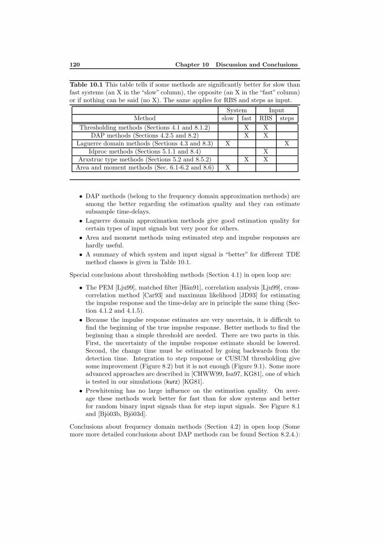
120 Chapter 10 Discussion and Conclusions
Table 10.1 This table tells if some methods are significantly better for slow thanfast systems (an X in the “slow” column), the opposite (an X in the “fast” column)or if nothing can be said (no X). The same applies for RBS and steps as input.
System InputMethod slow fast RBS steps
Thresholding methods (Sections 4.1 and 8.1.2) X XDAP methods (Sections 4.2.5 and 8.2) X X
Laguerre domain methods (Sections 4.3 and 8.3) X XIdproc methods (Sections 5.1.1 and 8.4) X
Arxstruc type methods (Sections 5.2 and 8.5.2) X XArea and moment methods (Sec. 6.1-6.2 and 8.6) X
• DAP methods (belong to the frequency domain approximation methods) areamong the better regarding the estimation quality and they can estimatesubsample time-delays.
• Laguerre domain approximation methods give good estimation quality forcertain types of input signals but very poor for others.
• Area and moment methods using estimated step and impulse responses arehardly useful.
• A summary of which system and input signal is “better” for different TDEmethod classes is given in Table 10.1.
Special conclusions about thresholding methods (Section 4.1) in open loop are:
• The PEM [Lju99], matched filter [Han91], correlation analysis [Lju99], cross-correlation method [Car93] and maximum likelihood [JD93] for estimatingthe impulse response and the time-delay are in principle the same thing (Sec-tion 4.1.2 and 4.1.5).
• Because the impulse response estimates are very uncertain, it is difficult tofind the beginning of the true impulse response. Better methods to find thebeginning than a simple threshold are needed. There are two parts in this.First, the uncertainty of the impulse response estimate should be lowered.Second, the change time must be estimated by going backwards from thedetection time. Integration to step response or CUSUM thresholding givesome improvement (Figure 8.2) but it is not enough (Figure 9.1). Some moreadvanced approaches are described in [CHWW99, Isa97, KG81], one of whichis tested in our simulations (kurz) [KG81].
• Prewhitening has no large influence on the estimation quality. On aver-age these methods work better for fast than for slow systems and betterfor random binary input signals than for step input signals. See Figure 8.1and [Bjo03b, Bjo03d].
Conclusions about frequency domain methods (Section 4.2) in open loop (Somemore more detailed conclusions about DAP methods can be found Section 8.2.4.):
10.3 Conclusions about Parameters and Properties of Methods 121
• Time-delay estimates relying on the allpass part of the system estimate canbe very incorrect if zeros of the system fall on the incorrect side of the stabilityboundary due to the noise (Section 4.2.6). A solution is to remove zeros nearthe stability boundary on the incorrect side (Section 4.2.7).
Conclusions about the Laguerre domain methods which are tested in this thesis(Section 4.3) in open loop (More detailed conclusions can be found in Section 8.3.6.):
• These methods are suitable for input signals which can be well approximatedby Laguerre functions, e.g. a few steps (Figures 4.12, 8.6 and 9.2 and re-port [Bjo03e]). Other types of input signals give very poor estimates.
• These methods give better time-delay estimates of systems with not too fastdynamics despite the fact these methods were derived for pure time-delaysystems (Figure 8.8 and report [Bjo03e]).
• The execution time is high but can be reduced if the same input signal isused in subsequent estimations (Section 8.3.4).
Conclusions about continuous-time one-step explicit methods (Section 5.1.1):
• For a first oder model with time-delay there is at most one minimum withineach sampling interval (Section 5.1.2). (There can be a single minimum inregion extending over several sampling intervals if LP-filtering is performed.See [FMS96] and Section 5.1.3)
• No matter how close to the true time-delay we start the optimization, thereare still cases which lead to an incorrect local minimum. Not even closeto the true time-delay, the Cramer Rao lower bound is always useful. SeeSection 5.1.2.
• Using no prewhitening of the input signal is best (Figure 8.9). On averagethese methods work better for random binary input signals than for stepinput signals (Figure 8.10) .
Conclusions about arxstruc type methods (Section 5.2) in open loop:
• High model orders are the best for arxstruc to be able to accurately describethe system and the noise (Section 8.5.1).
• The model orders for oestruc should be 1 for the numerator to avoid ambi-guity in the time-delay and be close to the true order for the denominator(Section 8.5.1).
• The prefiltered arxstruc, here called met1struc, has nearly as good estimationquality as oestruc but is much faster. If the true noise character is unchangedfor repeated time-delay estimations with met1struc, the execution speed isnearly as high as for arxstruc (Sections 8.5.1-8.5.2).
• On average these methods are better for fast than for slow systems (Fig. 9.3,8.14) and better for random binary input signals than for step input signals(Figures 9.2 and 8.14).
122 Chapter 10 Discussion and Conclusions
Conclusions about sampling methods (Section 5.3):
• It is possible to derive an explicit expression for the time-delay of a first ordersystem with time-delay after zero-order-hold sampling (Section 5.3.3).
Conclusions about area and moment methods utilizing estimated step and impulseresponses (Section 6.1) in open loop:
• Area and moment methods using estimated impulse and step responses oftenfail due to inaccurate estimates of the impulse and step responses (Section 8.6and report [Bjo03b]). (An improvement is described in [Ing03] but not tested
here. In [AH95] measured impulse and step responses are used but not here.
• Moment methods are less reliable than area methods and are not useful.
• On average these methods work better for slow systems than for fast systems(Section 8.6 and report [Bjo03b]). This is the opposite as for thresholdingmethods, which also use estimated impulse and step responses.
10.4 Future Work
Some interesting future work is:
• Make a better estimate of the change time in thresholding methods (Sec-tions 4.1.1 and 4.1.3) and test maximum likelihood based detection methods.
• Continue study of methods for separating the time-delay from the dynamics.See Section 4.1.1 and 4.1.4.
• Continue study of local minima in continuous and discrete-time one-step ex-plicit methods.
• Future work on sampling methods could be the following: Implement and testTIDEA (Section 5.3.2). Implement and test the method with exact time-delay from the sampling process (Section 5.3.3). This method uses a firstorder plus time-delay model structures. Derive the exact time-delay from thesampling process also for more complex model structures than first order plustime-delay, e.g. second order model with time-delay, and for first-order-holdsampling. A second order model structure as in idproc7 (Section 7.2) wouldprobably be better for the standard benchmark (Section 7.3.1).
• A comprehensive comparison of TDE methods on real data, for example: hairdryer [Lju99, p. 525], speech communication between driver and back seatpassenger in a car [Nyg03] or radar range estimation.
• Future work on applications, e.g. system identification for control; diagnosisand performance monitoring; direction of arrival estimation in signal intelli-gence, radar and mobile communications; and range estimation in radar.
Bibliography
[AH95] K. Astrom and T. Hagglund. PID Controllers: Theory, Design andTuning. Instrument Society of America, 2nd edition, 1995. ISBN1-55617-516-7.
[ASH84] K. J. Astrom, J. Sternby, and P. Hagander. Zeros of sampled systems.Automatica, 20(1):31–38, 1984.
[AW84] K. Astrom and B. Wittenmark. Computer Controlled Systems. Theoryand Design. Prentice-Hall, 1984.
[Bjo] S. Bjorklund. ESDATA. A Matlab toolbox for managing and analyz-ing data from factorial experiments. User’s guide. Technical ReportLiTH-ISY-R-xxxx, Department of Electrical Engineering, LinkopingUniversity, SE-581 83 Linkoping, Sweden. To be published.
[Bjo02] S. Bjorklund. Analysis of a phase method for time-delay estimation.Technical Report LiTH-ISY-R-2467, Department of Electrical Engi-neering, Linkoping University, SE-581 83 Linkoping, Sweden, October2002.
[Bjo03a] S. Bjorklund. Analysis of a phase method for time-delay estimation.Short version. Technical Report LiTH-ISY-R-2539, Department ofElectrical Engineering, Linkoping University, SE-581 83 Linkoping,Sweden, September 2003.
[Bjo03b] S. Bjorklund. Experimental evaluation of some cross correlation meth-ods for time-delay estimation in linear systems. Technical Report
123
124 Bibliography
LiTH-ISY-R-2513, Department of Electrical Engineering, LinkopingUniversity, SE-581 83 Linkoping, Sweden, April 2003.
[Bjo03c] S. Bjorklund. Experimental evaluation of some methods using simpleprocess models for estimating continuous time-delays in open-loop.Technical Report LiTH-ISY-R-2526, Department of Electrical Engi-neering, Linkoping University, SE-581 83 Linkoping, Sweden, July2003.
[Bjo03d] S. Bjorklund. Experimental evaluation of some thresholding methodsfor estimating time-delays in open-loop. Technical Report LiTH-ISY-R-2525, Department of Electrical Engineering, Linkoping University,SE-581 83 Linkoping, Sweden, July 2003.
[Bjo03e] S. Bjorklund. Experimental open-loop evaluation of some time-delayestimation methods in the Laguerre domain. Technical Report LiTH-ISY-R-2537, Department of Electrical Engineering, Linkoping Univer-sity, SE-581 83 Linkoping, Sweden, September 2003.
[Bjo03f] S. Bjorklund. A study of the choice of model orders in arxstruc-typemethods for open-loop time-delay estimation in linear systems. Tech-nical Report LiTH-ISY-R-2536, Department of Electrical Engineering,Linkoping University, SE-581 83 Linkoping, Sweden, August 2003.
[BL03] S. Bjorklund and L. Ljung. A review of time-delay estimation tech-niques. In Proceedings of the 42nd IEEE Conference on Decision andControl, Maui, Hawaii, USA, December 2003. To be published.
[BV03] S. Boyd and L. Vandenberghe. Convex Optimization. CambridgeUniversity Press, November 2003. Will be published in November2003, <http://www.stanford.edu/ boyd/cvxbook.html>.
[C+81] G. C. Carter et al. Special issue on time delay estimation. IEEETransactions on Acoustics, Speech and Signal Processing, 29(3), June1981. pt 2.
[Car87] G. C. Carter. Coherence and time delay estimation. Proceedings ofthe IEEE, 75(2):236–255, February 1987.
[Car93] G. Carter. Coherence and Time Delay Estimation - An Applied Tuto-rial for Research, Development, Test, and Evaluation Engineers. IEEEPress, 1993.
[CCS94] B.-S. Chen, J.-M. Chen, and S.-C. Shern. An ARMA robust systemidentification using a generalized lp norm estimation algorithm. IEEETransactions on Signal Processing, 42(5):1063–1073, May 1994.
Bibliography 125
[CHWW99] C. Carlemalm, S. Halvarsson, T. Wigren, and B. Wahlberg. Algo-rithms for time delay estimation using a low complexity exhaustivesearch. IEEE Transactions on Automatic Control, 44(5):1031–1037,May 1999.
[CST] CSTB. Matlab control system toolbox, v. 4.2.1 (R11.1). The Math-works Inc.
[DC02] K. De Cock. Principal Angles in System Theory, Information The-ory and Signal Processing. Phd thesis , Departement Elektrotech-niek, Katholieke Universiteit Leuven, Leuven-Heverlee, Belgium, 2002.ISBN 90-5682-351-5.
[EDE89] A. Elnaggar, G. A. Dumont, and A.-L. Elshafei. Recursive estimationfor system of unknown delay. In Proceedings of the 28th Conferenceon Decision and Control, Tampa, Florida, USA, December 1989.
[FHJ02] J. Falk, P. Handel, and M. Jansson. Direction finding for electronicwarfare systems using the phase of the cross spectral density. In Ra-dioVetenskap och Kommunikation (RVK), pages 264–268, June 2002.
[Fis99] B. R. Fischer. System Identification in Alternative Shift Operators withApplications and Some Other Topics. Phd thesis LTU-DT-99/18–SE,Department of Computer Science and Electrical Engineering, LuleaUniversity of Technology, Lulea, Sweden, August 1999.
[FM99a] B. R. Fischer and A. Medvedev. L2 time delay estimation by means ofLaguerre functions. In Proceedings of American Control Conference,San Diego, CA, USA, June 1999.
[FM99b] B. R. Fischer and A. Medvedev. Laguerre domain estimation of timedelays in narrowband ultrasonic echoes. In 14th Triennial IFAC WorldCongress, pages 361–366, Beijing, China, July 1999.
[FM99c] B. R. Fischer and A. Medvedev. Time delay estimation by meansof Laguerre functions. In 6th St. Petersburg Symposium on Adap-tive Systems Theory, volume 1, pages 65–68, St. Petersburg, Russia,September 1999.
[FMS91] G. Ferretti, C. Maffezzoni, and R. Scattolini. Recursive estimation oftime delay in sampled systems. Automatica, 27(4):653–661, 1991.
[FMS96] G. Ferretti, C. Maffezzoni, and R. Scattolini. On the identifiabilityof the time delay with least-squares methods. Automatica, 32(3):449–453, 1996.
[GL97] T. Glad and L. Ljung. Reglerteori. Flervariabla och olinjara metoder.Studentlitteratur, Lund, Sweden, 1997. In Swedish.
126 Bibliography
[GLM01] F. Gustafsson, L. Ljung, and M. Millnert. Signalbehandling. Stu-dentlitteratur, Lund, Sweden, 2001. In Swedish.
[GS94] A. Grennberg and M. Sandell. Estimation of subsample time delaydifferences in narrowband ultrasonic echoes using the hilbert trans-form correlation. IEEE Transactions on Ultrasonics, Ferroelectricsand Frequency Control, 41(5):588–595, September 1994.
[Gus00] F. Gustafsson. Adaptive Filtering and Change Detection. Wiley, 2000.ISBN 0-471-49287-6.
[GVL96] G. H. Golub and C. F. Van Loan. Matrix Computations. The JohnHopkins University Press, London, United Kingdom, 3rd edition,1996.
[Han91] E. Hansler. Statistische Signale. Grundlagen und Anwendungen.Springer Verlag, 1991.
[HJ91] R. A. Horn and C. R. Johnson. Topics in Matrix Analysis. CambridgeUniversity Press, 1991. ISBN 0-521-30587-X.
[Hor00] A. Horch. Condition Monitoring of Control Loops. Phd thesis TRITA-S3-REG-0002, Department of Signals, Sensors and Systems, RoyalInstitute of Technology, Stockholm, Sweden, 2000.
[HR95] A. W. Houghton and C. D. Reeve. Detection of spread-spectrum sig-nals using the time-domain filtered cross spectral density. IEE Pro-ceedings - Radar, Sonar and Navigation, 142(6):286–292, December1995.
[HR97] A. W. Houghton and C. D. Reeve. Direction finding on spread spec-trum signals using the time-domain filtered cross spectral density. IEEProceedings - Radar, Sonar and Navigation, 144(6):315–320, Decem-ber 1997.
[IHD00] A. J. Isaksson, A. Horch, and G. A. Dumont. Event-triggered deadtimeestimation – comparison of methods. In Preprints Control Systems2000, pages 209–215, Victoria, Canada, 2000.
[IHD01a] A. J. Isaksson, A. Horch, and G. A. Dumont. Event-triggered deadtimeestimation - comparison of methods. Technical report, Department ofSignals, Sensors & Systems, Royal Institute of Technology, Stockholm,Sweden, May 2001.
[IHD01b] A. J. Isaksson, A. Horch, and G. A. Dumont. Event-triggered deadtimeestimation from closed-loop data. In Proceedings of American ControlConference, Arlington, VA, USA, June 2001.
Bibliography 127
[Ing03] A. Ingimundarson. Dead-Time Compensation and Performance Mon-itoring in Process Control. Phd thesis, Dep. of Automatic Control,Lund Institute of Technology, Lund, Sweden, 2003.
[Isa97] M. Isaksson. A comparison of some approaches to time-delay esti-mation. Master’s thesis ISRN LUTFD2/TFRT–5580–SE, Dep. Auto-matic Control, Lund Institute of Technology, Sweden, 1997.
[JD93] D. H. Johnson and D. E. Dudgeon. Array Signal Processing. Conceptsand Techniques. Prentice Hall, 1993. ISBN 0-13-048513-6.
[Kau54] W. H. Kautz. Transient syntesis in the time domain. IRE Transactionson Circuit Theory, 1(3):29–39, September 1954.
[Kay93] S. M. Kay. Fundamentals of Statistical Signal Processing: EstimationTheory. Prentice-Hall, 1993. ISBN 0-13-042268-1.
[KG81] H. Kurz and W. Goedecke. Digital parameter-adaptive control of pro-cesses with unknown dead time. Automatica, 17:245–252, January1981.
[KQ92] S. Kingsley and S. Quegan. Understanding Radar Systems. McGraw-Hill, 1992. ISBN 0-07-707426-2.
[Kur79] H. Kurz. Digital parameter-adaptive control of processes with un-known constant or timevarying dead time. In Proceedings of the 5thIFAC Symposium on Identification and System Parameter Estimation,pages 1187–1194, Darmstadt, Germany, 1979.
[Lam93] J. Lam. Model reduction of delay systems using Pade approximants.International Journal of Control, 57(2):377–391, 1993.
[LG91] L. Ljung and T. Glad. Modellbygge och simulering. Studentlitteratur,Lund, Sweden, 1991. In Swedish.
[Lju99] L. Ljung. System Identification: Theory for the User. Prentice-Hall,Upper Saddle River, N.J. USA, 2nd edition, 1999.
[Lju02] L. Ljung. Identification for control: Simple process models. In Pro-ceedings of the 41st IEEE Conference on Decision and Control, pages4652–4657, Las Vegas, Nevada, USA, December 2002.
[Lju03] L. Ljung. System Identification Toolbox for use with Matlab. Version6. The MathWorks, Inc, Natick, MA, 6th edition, 2003.
[LT99] X. Lai and H. Torp. Interpolation methods for time-delay estimationusing cross-correlation method for blood velocity measurent. IEEETransactions on Ultrasonics, Ferroelectrics, and Frequency Control,46(2):277–290, March 1999.
128 Bibliography
[Mat96] Mathworks, Inc., 24 Prime Park Way, Natick, MA 01760-1500, USA.MATLAB Control System Toolbox. User’s Guide, December 1996.
[Mat98] Mathworks, Inc., 24 Prime Park Way, Natick, MA 01760-1500, USA.MATLAB Higher-Order Spectral Analysis Toolbox. User’s Guide, Jan-uary 1998.
[Mat01] The MathWorks, Inc. MATLAB Statistics Toolbox. User’s Guide. Ver-sion 3, 2001.
[MG+98] H. Messer, J. Goldberg, et al. Highlights of statistical signal and arrayprocessing. IEEE Signal Processing Magazine, pages 21–64, September1998.
[Mod91] Moddemeijer. On the determination of the position of extrema of sam-pled correlators. IEEE Transactions on Signal Processing, 39(1):216–219, January 1991.
[Mon97] D. C. Montgomery. Design and Analysis of Experiments. Wiley, 1997.ISBN 0-471-15746-5.
[MZJ87] M. Malek-Zavarei and M. Jamshidi. Time-Delay Systems. Analysis,Optimization and Applications. Elsevier Science Publishers B.V., Am-sterdam, The Netherlands, 1987. ISBN 0-444-70204-0.
[NL91] P. Nagy and L. Ljung. Estimating time-delays via state-space identifi-cation methods. In Preprints 9th IFAC Symposium on System Identifi-cation and System Parameter Estimation, pages 1141–1144, Budapest,Hungary, Jul 1991.
[NM93] C. L. Nikias and J. M. Mendel. Signal processing with higher-orderspectra. IEEE Signal Processing Magazine, pages 10–37, July 1993.
[NP88] C. L. Nikias and R. Pan. Time delay estimation in unknown gaussianspatially correlated noise. IEEE Transactions on Acoustics, Speech,and Signal Processing, 36(11):1706–1714, November 1988.
[NS95] D. T. Nagle and J. Saniie. Performance analysis of linearly combinedorder statistic cfar detectors. IEEE Transactions on Aerospace andElectronic Systems, 31(2):522–533, April 1995.
[Nyg03] M. Nygren. Improved speech communication in a car. Master’s the-sis LiTH-ISY-EX-3397-2003, Department of Electrical Engineering,Linkoping University, Linkoping, Sweden, June 2003.
[Pag54] E. S. Page. Continuous inspection schemes. Biometrika, 41:100–115,1954.
Bibliography 129
[Pup85] R. Pupeikis. Recursive estimation of the parameters of linear systemswith time delay. In Proc. 7th IFAC/IFORS Symp. Identification andSystem Parameter Estimation, pages 787–792, York, UK, July 1985.
[Qua81] A. H. Quazi. An overview on the time delay estimate in active and pas-sive systems for target localization. IEEE Transactions on Acoustics,Speech and Signal Processing, 29(3):527–533, June 1981. pt. 2.
[SBS97] A. Soumelidis, J. Bokor, and F. Schipp. Representation and approxi-mation of signals and systems using Generalized Kautz Functions. InProceedings of the 36th Conference on Decision and Control, pages3793–, San Diego, California, USA, December 1997.
[SIT] SITB. Matlab system identification toolbox v. 5.0.1 (R12.1). TheMathworks Inc.
[Sum95] A. Sume. Kursmaterial i radarteori. Technical Report FOA-D–95-00108-3.3-SE, Department of Sensor Technology, Swedish Defence Re-search Establishment, Box 1165, 581 11 Linkoping, Sweden, April1995. In Swedish.
[Swa99] A. P. Swanda. PID Controller Performance Assessment Based onClosed-Loop Response Data. Phd thesis, University of California,Santa Barbara, California, USA, June 1999.
[Wah91] B. Wahlberg. System identification using Laguerre models. IEEETransactions on Automatic Control, AC-36(5):551–562, May 1991.
[Wah94] B. Wahlberg. System identification using Kautz models. IEEE Trans-actions on Automatic Control, 39(6):1276–1282, June 1994.
[Wik02] M. Wikstrom. Utveckling och implementering av ett audiopejlsystembaserat pa tidsdifferensmatning. Master’s thesis LiTH-ISY-EX-3277-2002, Linkopings universitet, Linkoping, Sweden, October 2002. Inswedish.
[WZ01] Q.-G. Wang and Y. Zhang. Robust identification of continuous sys-tems with dead-time from step responses. Automatica, pages 377–390,2001.

130 Bibliography
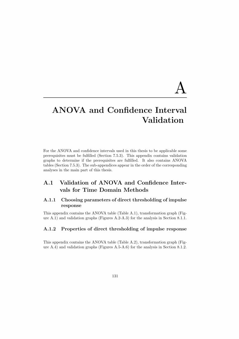
AANOVA and Confidence Interval
Validation
For the ANOVA and confidence intervals used in this thesis to be applicable someprerequisites must be fulfilled (Section 7.5.3). This appendix contains validationgraphs to determine if the prerequisites are fulfilled. It also contains ANOVAtables (Section 7.5.3). The sub-appendices appear in the order of the correspondinganalyses in the main part of this thesis.
A.1 Validation of ANOVA and Confidence Inter-vals for Time Domain Methods
A.1.1 Choosing parameters of direct thresholding of impulseresponse
This appendix contains the ANOVA table (Table A.1), transformation graph (Fig-ure A.1) and validation graphs (Figures A.2-A.3) for the analysis in Section 8.1.1.
A.1.2 Properties of direct thresholding of impulse response
This appendix contains the ANOVA table (Table A.2), transformation graph (Fig-ure A.4) and validation graphs (Figures A.5-A.6) for the analysis in Section 8.1.2.
131
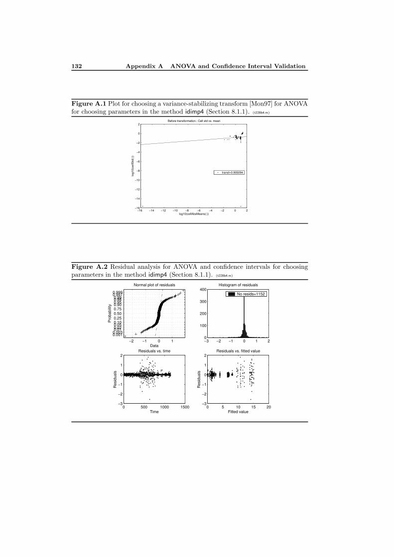
132 Appendix A ANOVA and Confidence Interval Validation
Figure A.1 Plot for choosing a variance-stabilizing transform [Mon97] for ANOVAfor choosing parameters in the method idimp4 (Section 8.1.1). (t228b4.m)
−16 −14 −12 −10 −8 −6 −4 −2 0 2−16
−14
−12
−10
−8
−6
−4
−2
0
2
log10(cellAbsMeans(:))
log1
0(ce
llStd
(:))
Before transformation.: Cell std vs. mean
transf=0.905094
PSfrag replacements
tu(t)y(t)s(t)
gts(t)
TdTd
δ(t− Td)g(t)gr(t)g(t)
w(t)r(t)e(t)u(t)y(t)v(t)H(s)F (s)G(s)
Figure A.2 Residual analysis for ANOVA and confidence intervals for choosingparameters in the method idimp4 (Section 8.1.1). (t228b4.m)
−2 −1 0 1
0.0010.0030.01 0.02 0.05 0.10 0.25 0.50 0.75 0.90 0.95 0.98 0.99
0.9970.999
Data
Pro
babi
lity
Normal plot of residuals
−3 −2 −1 0 1 20
100
200
300
400Histogram of residuals
No resids=1152
0 500 1000 1500−3
−2
−1
0
1
2Residuals vs. time
Time
Res
idua
ls
0 5 10 15 20−3
−2
−1
0
1
2Residuals vs. fitted value
Fitted value
Res
idua
ls
PSfrag replacements
tu(t)y(t)s(t)
gts(t)
TdTd
δ(t− Td)g(t)gr(t)g(t)
w(t)r(t)e(t)u(t)y(t)v(t)H(s)F (s)G(s)
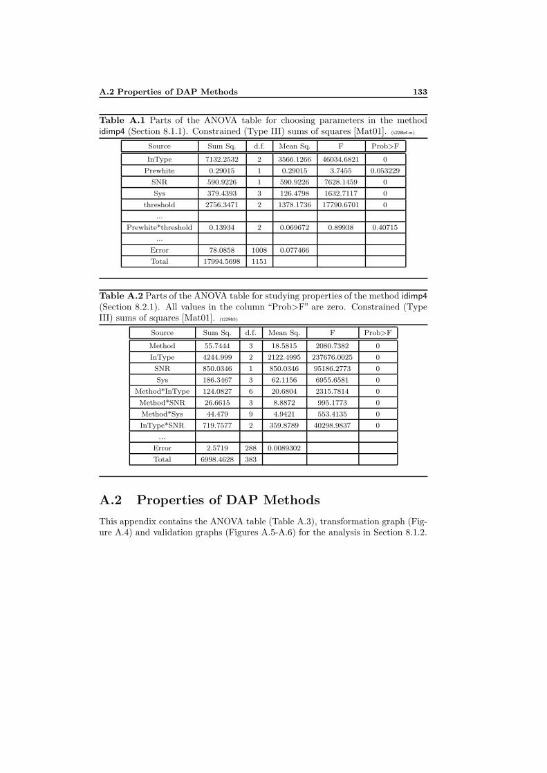
A.2 Properties of DAP Methods 133
Table A.1 Parts of the ANOVA table for choosing parameters in the methodidimp4 (Section 8.1.1). Constrained (Type III) sums of squares [Mat01]. (t228b4.m)
Source Sum Sq. d.f. Mean Sq. F Prob>F
InType 7132.2532 2 3566.1266 46034.6821 0
Prewhite 0.29015 1 0.29015 3.7455 0.053229
SNR 590.9226 1 590.9226 7628.1459 0
Sys 379.4393 3 126.4798 1632.7117 0
threshold 2756.3471 2 1378.1736 17790.6701 0
...
Prewhite*threshold 0.13934 2 0.069672 0.89938 0.40715
...
Error 78.0858 1008 0.077466
Total 17994.5698 1151
Table A.2 Parts of the ANOVA table for studying properties of the method idimp4(Section 8.2.1). All values in the column “Prob>F” are zero. Constrained (TypeIII) sums of squares [Mat01]. (t229b5)
Source Sum Sq. d.f. Mean Sq. F Prob>F
Method 55.7444 3 18.5815 2080.7382 0
InType 4244.999 2 2122.4995 237676.0025 0
SNR 850.0346 1 850.0346 95186.2773 0
Sys 186.3467 3 62.1156 6955.6581 0
Method*InType 124.0827 6 20.6804 2315.7814 0
Method*SNR 26.6615 3 8.8872 995.1773 0
Method*Sys 44.479 9 4.9421 553.4135 0
InType*SNR 719.7577 2 359.8789 40298.9837 0
...Error 2.5719 288 0.0089302
Total 6998.4628 383
A.2 Properties of DAP Methods
This appendix contains the ANOVA table (Table A.3), transformation graph (Fig-ure A.4) and validation graphs (Figures A.5-A.6) for the analysis in Section 8.1.2.
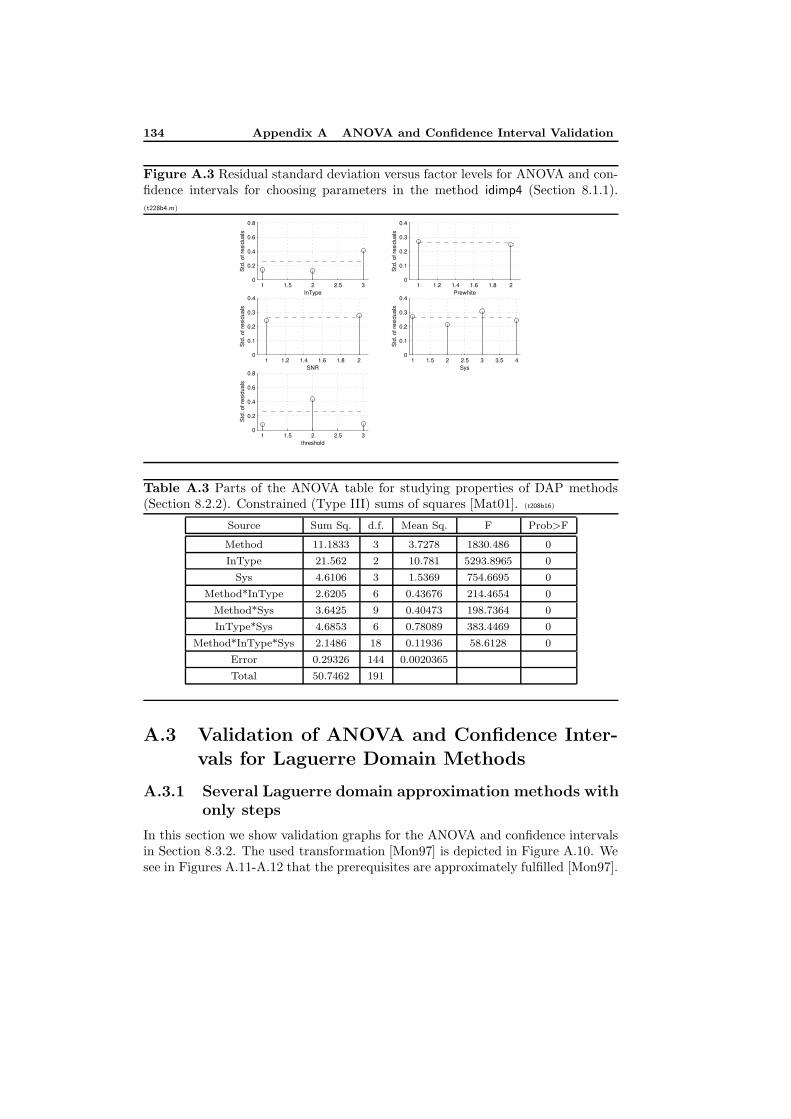
134 Appendix A ANOVA and Confidence Interval Validation
Figure A.3 Residual standard deviation versus factor levels for ANOVA and con-fidence intervals for choosing parameters in the method idimp4 (Section 8.1.1).(t228b4.m)
1 1.5 2 2.5 30
0.2
0.4
0.6
0.8
InType
Std
. of r
esid
uals
1 1.2 1.4 1.6 1.8 20
0.1
0.2
0.3
0.4
Prewhite
Std
. of r
esid
uals
1 1.2 1.4 1.6 1.8 20
0.1
0.2
0.3
0.4
SNR
Std
. of r
esid
uals
1 1.5 2 2.5 3 3.5 40
0.1
0.2
0.3
0.4
Sys
Std
. of r
esid
uals
1 1.5 2 2.5 30
0.2
0.4
0.6
0.8
threshold
Std
. of r
esid
uals
PSfrag replacements
tu(t)y(t)s(t)
gts(t)
TdTd
δ(t− Td)g(t)gr(t)g(t)
w(t)r(t)e(t)u(t)y(t)v(t)H(s)F (s)G(s)
Table A.3 Parts of the ANOVA table for studying properties of DAP methods(Section 8.2.2). Constrained (Type III) sums of squares [Mat01]. (t208b16)
Source Sum Sq. d.f. Mean Sq. F Prob>F
Method 11.1833 3 3.7278 1830.486 0
InType 21.562 2 10.781 5293.8965 0
Sys 4.6106 3 1.5369 754.6695 0
Method*InType 2.6205 6 0.43676 214.4654 0
Method*Sys 3.6425 9 0.40473 198.7364 0
InType*Sys 4.6853 6 0.78089 383.4469 0
Method*InType*Sys 2.1486 18 0.11936 58.6128 0
Error 0.29326 144 0.0020365
Total 50.7462 191
A.3 Validation of ANOVA and Confidence Inter-
vals for Laguerre Domain Methods
A.3.1 Several Laguerre domain approximation methods withonly steps
In this section we show validation graphs for the ANOVA and confidence intervalsin Section 8.3.2. The used transformation [Mon97] is depicted in Figure A.10. Wesee in Figures A.11-A.12 that the prerequisites are approximately fulfilled [Mon97].
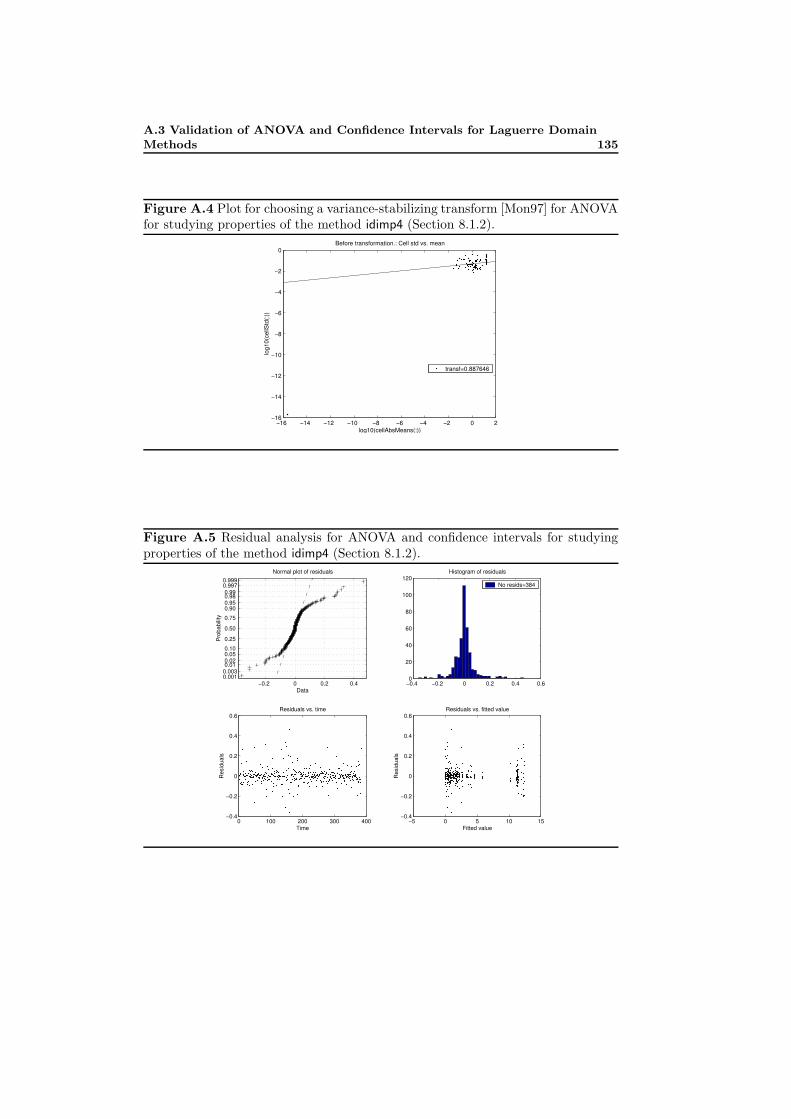
A.3 Validation of ANOVA and Confidence Intervals for Laguerre DomainMethods 135
Figure A.4 Plot for choosing a variance-stabilizing transform [Mon97] for ANOVAfor studying properties of the method idimp4 (Section 8.1.2).
−16 −14 −12 −10 −8 −6 −4 −2 0 2−16
−14
−12
−10
−8
−6
−4
−2
0
log10(cellAbsMeans(:))
log1
0(ce
llStd
(:))
Before transformation.: Cell std vs. mean
transf=0.887646
PSfrag replacements
tu(t)y(t)s(t)
gts(t)
TdTd
δ(t− Td)g(t)gr(t)g(t)
w(t)r(t)e(t)u(t)y(t)v(t)H(s)F (s)G(s)
Figure A.5 Residual analysis for ANOVA and confidence intervals for studyingproperties of the method idimp4 (Section 8.1.2).
−0.2 0 0.2 0.40.0010.0030.01 0.02 0.05 0.10
0.25
0.50
0.75
0.90 0.95 0.98 0.99
0.9970.999
Data
Pro
babi
lity
Normal plot of residuals
−0.4 −0.2 0 0.2 0.4 0.60
20
40
60
80
100
120Histogram of residuals
No resids=384
0 100 200 300 400−0.4
−0.2
0
0.2
0.4
0.6Residuals vs. time
Time
Res
idua
ls
−5 0 5 10 15−0.4
−0.2
0
0.2
0.4
0.6Residuals vs. fitted value
Fitted value
Res
idua
ls
PSfrag replacements
tu(t)y(t)s(t)
gts(t)
TdTd
δ(t− Td)g(t)gr(t)g(t)
w(t)r(t)e(t)u(t)y(t)v(t)H(s)F (s)G(s)
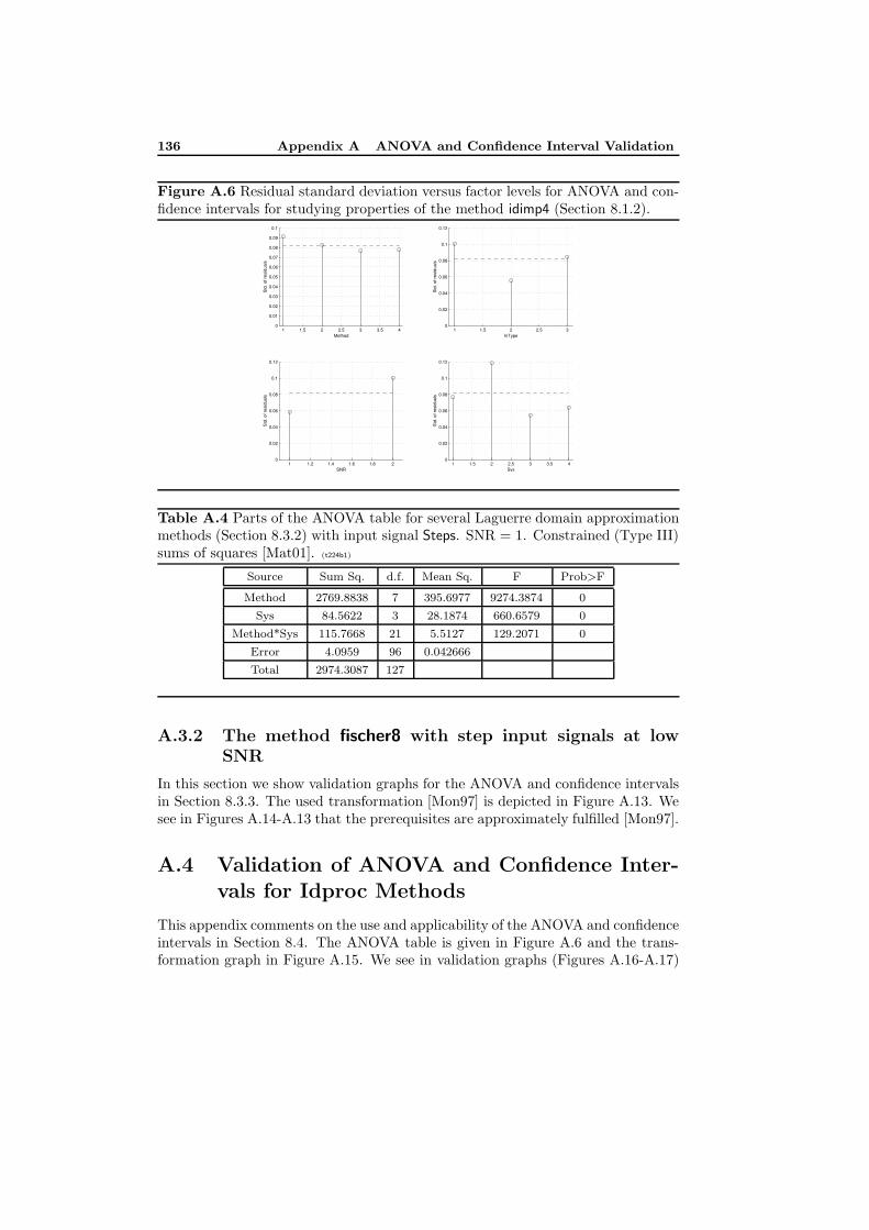
136 Appendix A ANOVA and Confidence Interval Validation
Figure A.6 Residual standard deviation versus factor levels for ANOVA and con-fidence intervals for studying properties of the method idimp4 (Section 8.1.2).
1 1.5 2 2.5 3 3.5 40
0.01
0.02
0.03
0.04
0.05
0.06
0.07
0.08
0.09
0.1
Method
Std
. of r
esid
uals
1 1.5 2 2.5 30
0.02
0.04
0.06
0.08
0.1
0.12
InType
Std
. of r
esid
uals
1 1.2 1.4 1.6 1.8 20
0.02
0.04
0.06
0.08
0.1
0.12
SNR
Std
. of r
esid
uals
1 1.5 2 2.5 3 3.5 40
0.02
0.04
0.06
0.08
0.1
0.12
Sys
Std
. of r
esid
uals
PSfrag replacements
tu(t)y(t)s(t)
gts(t)
TdTd
δ(t− Td)g(t)gr(t)g(t)
w(t)r(t)e(t)u(t)y(t)v(t)H(s)F (s)G(s)
Table A.4 Parts of the ANOVA table for several Laguerre domain approximationmethods (Section 8.3.2) with input signal Steps. SNR = 1. Constrained (Type III)sums of squares [Mat01]. (t224b1)
Source Sum Sq. d.f. Mean Sq. F Prob>F
Method 2769.8838 7 395.6977 9274.3874 0
Sys 84.5622 3 28.1874 660.6579 0
Method*Sys 115.7668 21 5.5127 129.2071 0
Error 4.0959 96 0.042666
Total 2974.3087 127
A.3.2 The method fischer8 with step input signals at lowSNR
In this section we show validation graphs for the ANOVA and confidence intervalsin Section 8.3.3. The used transformation [Mon97] is depicted in Figure A.13. Wesee in Figures A.14-A.13 that the prerequisites are approximately fulfilled [Mon97].
A.4 Validation of ANOVA and Confidence Inter-vals for Idproc Methods
This appendix comments on the use and applicability of the ANOVA and confidenceintervals in Section 8.4. The ANOVA table is given in Figure A.6 and the trans-formation graph in Figure A.15. We see in validation graphs (Figures A.16-A.17)
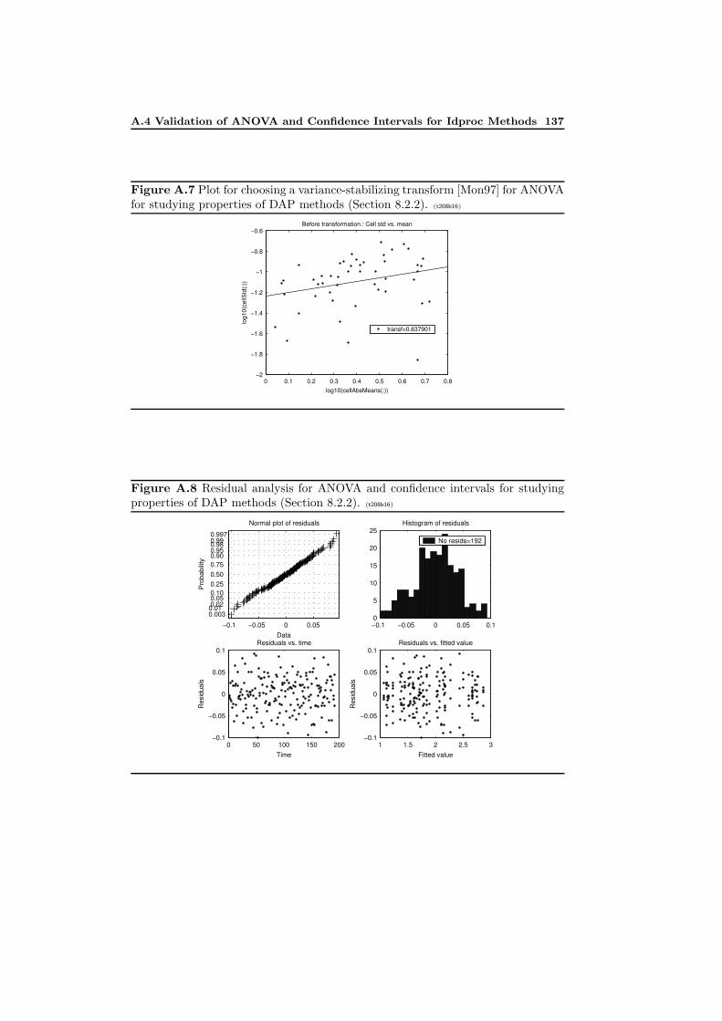
A.4 Validation of ANOVA and Confidence Intervals for Idproc Methods 137
Figure A.7 Plot for choosing a variance-stabilizing transform [Mon97] for ANOVAfor studying properties of DAP methods (Section 8.2.2). (t208b16)
0 0.1 0.2 0.3 0.4 0.5 0.6 0.7 0.8−2
−1.8
−1.6
−1.4
−1.2
−1
−0.8
−0.6
log10(cellAbsMeans(:))
log1
0(ce
llStd
(:))
Before transformation.: Cell std vs. mean
transf=0.637901
PSfrag replacements
tu(t)y(t)s(t)
gts(t)
TdTd
δ(t− Td)g(t)gr(t)g(t)
w(t)r(t)e(t)u(t)y(t)v(t)H(s)F (s)G(s)
Figure A.8 Residual analysis for ANOVA and confidence intervals for studyingproperties of DAP methods (Section 8.2.2). (t208b16)
−0.1 −0.05 0 0.05
0.0030.01 0.02 0.05 0.10 0.25 0.50 0.75 0.90 0.95 0.98 0.99 0.997
Data
Pro
babi
lity
Normal plot of residuals
−0.1 −0.05 0 0.05 0.10
5
10
15
20
25Histogram of residuals
No resids=192
0 50 100 150 200−0.1
−0.05
0
0.05
0.1Residuals vs. time
Time
Res
idua
ls
1 1.5 2 2.5 3−0.1
−0.05
0
0.05
0.1Residuals vs. fitted value
Fitted value
Res
idua
ls
PSfrag replacements
tu(t)y(t)s(t)
gts(t)
TdTd
δ(t− Td)g(t)gr(t)g(t)
w(t)r(t)e(t)u(t)y(t)v(t)H(s)F (s)G(s)
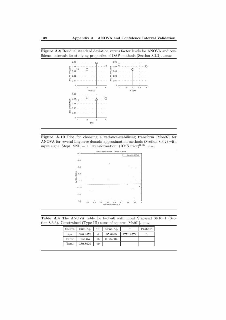
138 Appendix A ANOVA and Confidence Interval Validation
Figure A.9 Residual standard deviation versus factor levels for ANOVA and con-fidence intervals for studying properties of DAP methods (Section 8.2.2). (t208b16)
1 2 3 40
0.01
0.02
0.03
0.04
0.05
Method
Std
. of r
esid
uals
1 1.5 2 2.5 30
0.01
0.02
0.03
0.04
0.05
InType
Std
. of r
esid
uals
1 2 3 40
0.01
0.02
0.03
0.04
0.05
Sys
Std
. of r
esid
uals
PSfrag replacements
tu(t)y(t)s(t)
gts(t)
TdTd
δ(t− Td)g(t)gr(t)g(t)
w(t)r(t)e(t)u(t)y(t)v(t)H(s)F (s)G(s)
Figure A.10 Plot for choosing a variance-stabilizing transform [Mon97] forANOVA for several Laguerre domain approximation methods (Section 8.3.2) withinput signal Steps. SNR = 1. Transformation: (RMS error)0.96. (t224b1)
0.1 0.2 0.3 0.4 0.5 0.6 0.7 0.8 0.9 1−1.6
−1.4
−1.2
−1
−0.8
−0.6
−0.4
−0.2
log10(cellAbsMeans(:))
log1
0(ce
llStd
(:))
Before transformation.: Cell std vs. mean
transf=0.957842
PSfrag replacements
tu(t)y(t)s(t)
gts(t)
TdTd
δ(t− Td)g(t)gr(t)g(t)
w(t)r(t)e(t)u(t)y(t)v(t)H(s)F (s)G(s)
Table A.5 The ANOVA table for fischer8 with input Stepsand SNR=1 (Sec-tion 8.3.3). Constrained (Type III) sums of squares [Mat01]. (t225b1)
Source Sum Sq. d.f. Mean Sq. F Prob>F
Sys 380.3476 4 95.0869 2771.8578 0
Error 0.51457 15 0.034304
Total 380.8622 19
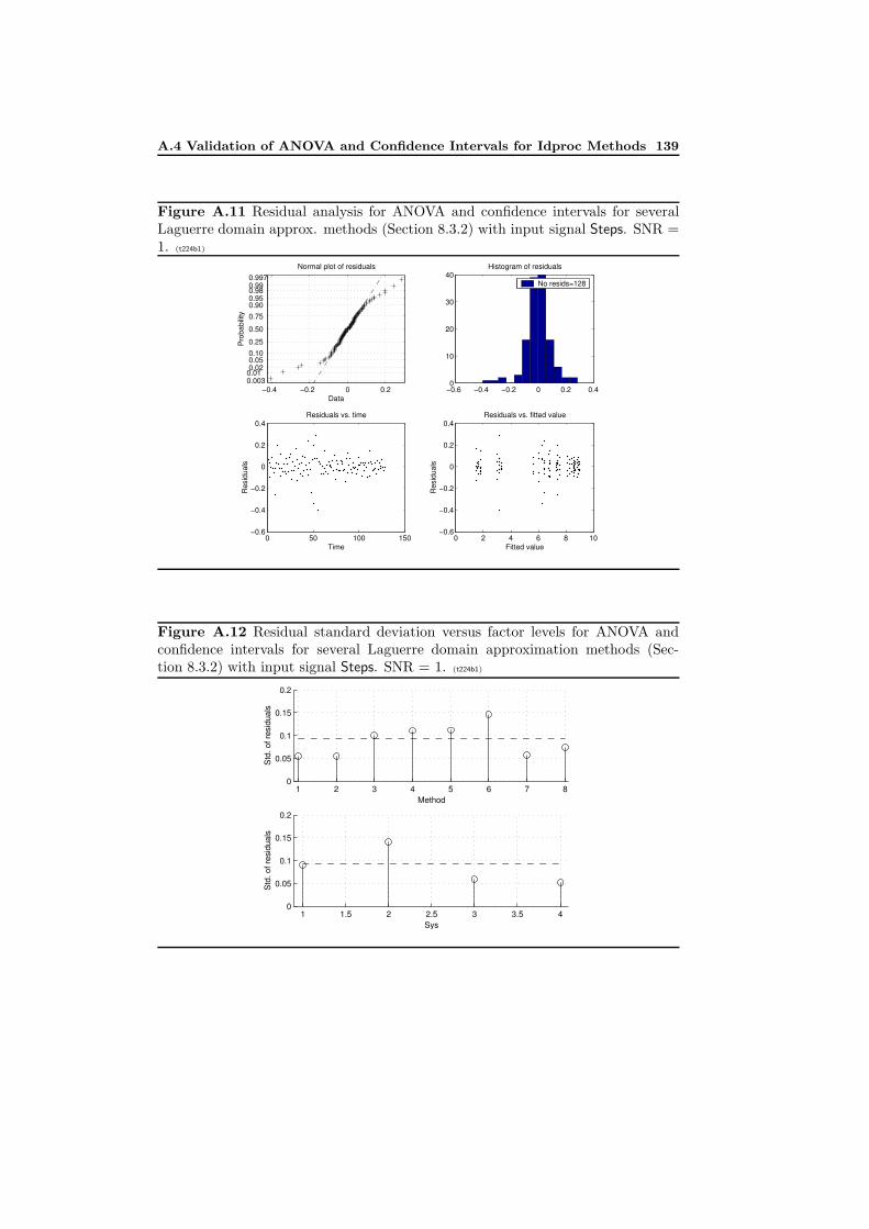
A.4 Validation of ANOVA and Confidence Intervals for Idproc Methods 139
Figure A.11 Residual analysis for ANOVA and confidence intervals for severalLaguerre domain approx. methods (Section 8.3.2) with input signal Steps. SNR =1. (t224b1)
−0.4 −0.2 0 0.20.0030.01 0.02 0.05 0.10 0.25
0.50
0.75 0.90 0.95 0.98 0.99 0.997
Data
Pro
babi
lity
Normal plot of residuals
−0.6 −0.4 −0.2 0 0.2 0.40
10
20
30
40Histogram of residuals
No resids=128
0 50 100 150−0.6
−0.4
−0.2
0
0.2
0.4Residuals vs. time
Time
Res
idua
ls
0 2 4 6 8 10−0.6
−0.4
−0.2
0
0.2
0.4Residuals vs. fitted value
Fitted value
Res
idua
ls
PSfrag replacements
tu(t)y(t)s(t)
gts(t)
TdTd
δ(t− Td)g(t)gr(t)g(t)
w(t)r(t)e(t)u(t)y(t)v(t)H(s)F (s)G(s)
Figure A.12 Residual standard deviation versus factor levels for ANOVA andconfidence intervals for several Laguerre domain approximation methods (Sec-tion 8.3.2) with input signal Steps. SNR = 1. (t224b1)
1 2 3 4 5 6 7 80
0.05
0.1
0.15
0.2
Method
Std
. of r
esid
uals
1 1.5 2 2.5 3 3.5 40
0.05
0.1
0.15
0.2
Sys
Std
. of r
esid
uals
PSfrag replacements
tu(t)y(t)s(t)
gts(t)
TdTd
δ(t− Td)g(t)gr(t)g(t)
w(t)r(t)e(t)u(t)y(t)v(t)H(s)F (s)G(s)
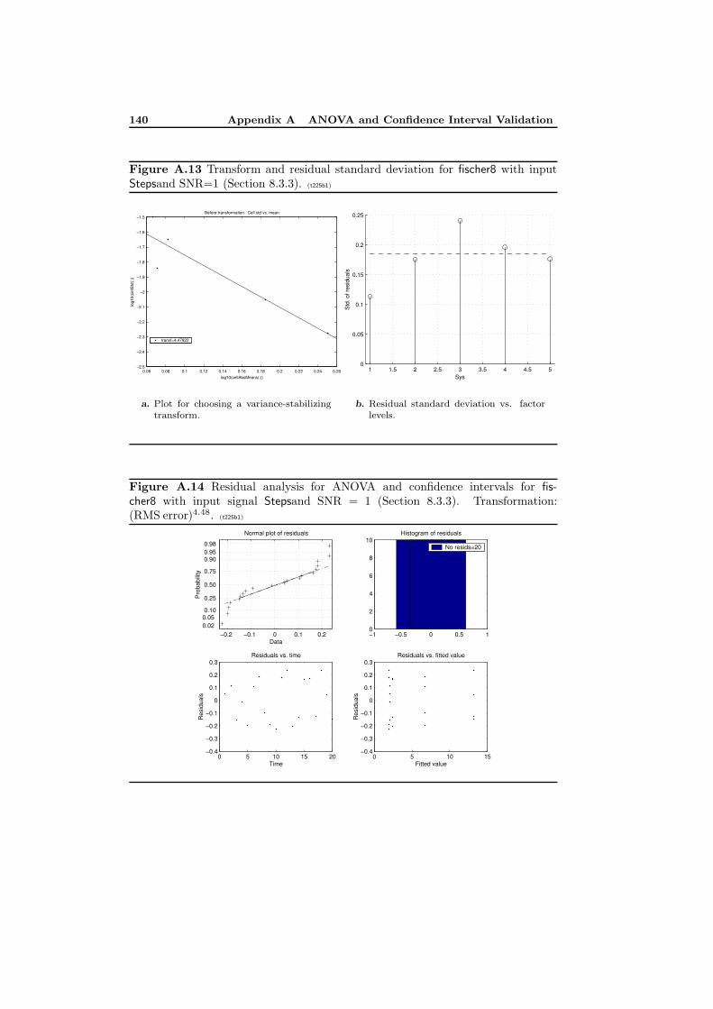
140 Appendix A ANOVA and Confidence Interval Validation
Figure A.13 Transform and residual standard deviation for fischer8 with inputStepsand SNR=1 (Section 8.3.3). (t225b1)
0.06 0.08 0.1 0.12 0.14 0.16 0.18 0.2 0.22 0.24 0.26−2.5
−2.4
−2.3
−2.2
−2.1
−2
−1.9
−1.8
−1.7
−1.6
−1.5
log10(cellAbsMeans(:))
log1
0(ce
llStd
(:))
Before transformation.: Cell std vs. mean
transf=4.47922
PSfrag replacements
tu(t)y(t)s(t)
gts(t)
TdTd
δ(t− Td)g(t)gr(t)g(t)
w(t)r(t)e(t)u(t)y(t)v(t)H(s)F (s)G(s)
a. Plot for choosing a variance-stabilizingtransform.
1 1.5 2 2.5 3 3.5 4 4.5 50
0.05
0.1
0.15
0.2
0.25
Sys
Std
. of r
esid
uals
PSfrag replacements
tu(t)y(t)s(t)
gts(t)
TdTd
δ(t− Td)g(t)gr(t)g(t)
w(t)r(t)e(t)u(t)y(t)v(t)H(s)F (s)G(s)
b. Residual standard deviation vs. factorlevels.
Figure A.14 Residual analysis for ANOVA and confidence intervals for fis-cher8 with input signal Stepsand SNR = 1 (Section 8.3.3). Transformation:(RMS error)4.48. (t225b1)
−0.2 −0.1 0 0.1 0.20.02 0.05 0.10
0.25
0.50
0.75
0.90 0.95 0.98
Data
Pro
babi
lity
Normal plot of residuals
−1 −0.5 0 0.5 10
2
4
6
8
10Histogram of residuals
No resids=20
0 5 10 15 20−0.4
−0.3
−0.2
−0.1
0
0.1
0.2
0.3Residuals vs. time
Time
Res
idua
ls
0 5 10 15−0.4
−0.3
−0.2
−0.1
0
0.1
0.2
0.3Residuals vs. fitted value
Fitted value
Res
idua
ls
PSfrag replacements
tu(t)y(t)s(t)
gts(t)
TdTd
δ(t− Td)g(t)gr(t)g(t)
w(t)r(t)e(t)u(t)y(t)v(t)H(s)F (s)G(s)
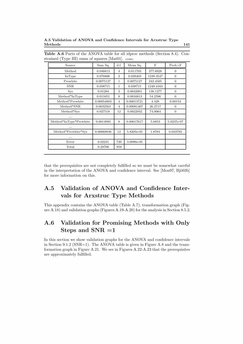
A.5 Validation of ANOVA and Confidence Intervals for Arxstruc TypeMethods 141
Table A.6 Parts of the ANOVA table for all idproc methods (Section 8.4). Con-strained (Type III) sums of squares [Mat01]. (t233b2)
Source Sum Sq. d.f. Mean Sq. F Prob>F
Method 0.046813 4 0.011703 377.6928 0
InType 0.076806 2 0.038403 1239.3547 0
Prewhite 0.0075127 1 0.0075127 242.4505 0
SNR 0.038715 1 0.038715 1249.4163 0
Sys 0.01284 3 0.0042801 138.1277 0
Method*InType 0.013451 8 0.0016813 54.2596 0
Method*Prewhite 0.00054883 4 0.00013721 4.428 0.00153
Method*SNR 0.0032563 4 0.00081407 26.2717 0
Method*Sys 0.027518 12 0.0022932 74.0064 0
...Method*InType*Prewhite 0.0014093 8 0.00017617 5.6853 5.0237e-07
...Method*Prewhite*Sys 0.00069846 12 5.8205e-05 1.8784 0.033792
...Error 0.02231 720 3.0986e-05
Total 0.29706 959
that the prerequisites are not completely fulfilled so we must be somewhat carefulin the interpretation of the ANOVA and confidence interval. See [Mon97, Bjo03b]for more information on this.
A.5 Validation of ANOVA and Confidence Inter-vals for Arxstruc Type Methods
This appendix contains the ANOVA table (Table A.7), transformation graph (Fig-ure A.18) and validation graphs (Figures A.19-A.20) for the analysis in Section 8.5.2.
A.6 Validation for Promising Methods with Only
Steps and SNR =1
In this section we show validation graphs for the ANOVA and confidence intervalsin Section 9.1.2 (SNR=1). The ANOVA table is given in Figure A.8 and the trans-formation graph in Figure A.21. We see in Figures A.22-A.23 that the prerequisitesare approximately fulfilled.
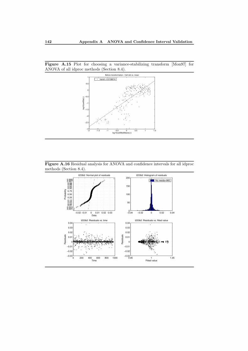
142 Appendix A ANOVA and Confidence Interval Validation
Figure A.15 Plot for choosing a variance-stabilizing transform [Mon97] forANOVA of all idproc methods (Section 8.4).
−2 −1.5 −1 −0.5 0 0.5 1 1.5−3
−2.5
−2
−1.5
−1
−0.5
0
0.5
1
log10(cellAbsMeans(:))
log1
0(ce
llStd
(:))
Before transformation.: Cell std vs. mean
transf=−0.0108014
PSfrag replacements
tu(t)y(t)s(t)
gts(t)
TdTd
δ(t− Td)g(t)gr(t)g(t)
w(t)r(t)e(t)u(t)y(t)v(t)H(s)F (s)G(s)
Figure A.16 Residual analysis for ANOVA and confidence intervals for all idprocmethods (Section 8.4).
−0.02 −0.01 0 0.01 0.02 0.03
0.0010.0030.01 0.02 0.05 0.10 0.25 0.50 0.75 0.90 0.95 0.98 0.99
0.9970.999
Data
Pro
babi
lity
t233b2 :Normal plot of residuals
−0.04 −0.02 0 0.02 0.040
50
100
150
200t233b2 :Histogram of residuals
No resids=960
0 200 400 600 800 1000−0.03
−0.02
−0.01
0
0.01
0.02
0.03
0.04t233b2 :Residuals vs. time
Time
Res
idua
ls
0.95 1 1.05−0.03
−0.02
−0.01
0
0.01
0.02
0.03
0.04t233b2 :Residuals vs. fitted value
Fitted value
Res
idua
ls
PSfrag replacements
tu(t)y(t)s(t)
gts(t)
TdTd
δ(t− Td)g(t)gr(t)g(t)
w(t)r(t)e(t)u(t)y(t)v(t)H(s)F (s)G(s)
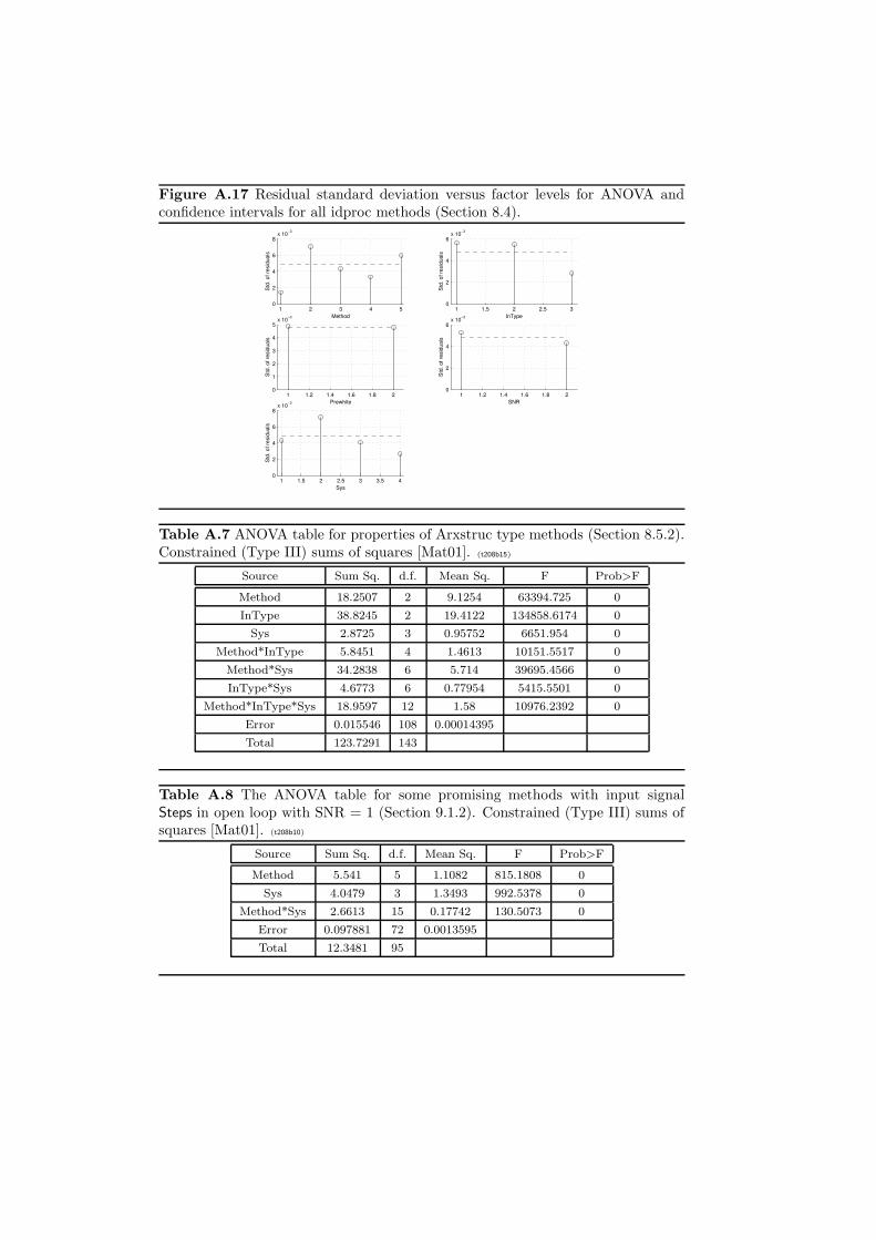
Figure A.17 Residual standard deviation versus factor levels for ANOVA andconfidence intervals for all idproc methods (Section 8.4).
1 2 3 4 50
2
4
6
8x 10⁻³
Method
Std
. of r
esid
uals
1 1.5 2 2.5 30
2
4
6x 10⁻³
InType
Std
. of r
esid
uals
1 1.2 1.4 1.6 1.8 20
1
2
3
4
5x 10⁻³
Prewhite
Std
. of r
esid
uals
1 1.2 1.4 1.6 1.8 20
2
4
6x 10⁻³
SNR
Std
. of r
esid
uals
1 1.5 2 2.5 3 3.5 40
2
4
6
8x 10⁻³
Sys
Std
. of r
esid
uals
PSfrag replacements
tu(t)y(t)s(t)
gts(t)
TdTd
δ(t− Td)g(t)gr(t)g(t)
w(t)r(t)e(t)u(t)y(t)v(t)H(s)F (s)G(s)
Table A.7 ANOVA table for properties of Arxstruc type methods (Section 8.5.2).Constrained (Type III) sums of squares [Mat01]. (t208b15)
Source Sum Sq. d.f. Mean Sq. F Prob>F
Method 18.2507 2 9.1254 63394.725 0
InType 38.8245 2 19.4122 134858.6174 0
Sys 2.8725 3 0.95752 6651.954 0
Method*InType 5.8451 4 1.4613 10151.5517 0
Method*Sys 34.2838 6 5.714 39695.4566 0
InType*Sys 4.6773 6 0.77954 5415.5501 0
Method*InType*Sys 18.9597 12 1.58 10976.2392 0
Error 0.015546 108 0.00014395
Total 123.7291 143
Table A.8 The ANOVA table for some promising methods with input signalSteps in open loop with SNR = 1 (Section 9.1.2). Constrained (Type III) sums ofsquares [Mat01]. (t208b10)
Source Sum Sq. d.f. Mean Sq. F Prob>F
Method 5.541 5 1.1082 815.1808 0
Sys 4.0479 3 1.3493 992.5378 0
Method*Sys 2.6613 15 0.17742 130.5073 0
Error 0.097881 72 0.0013595
Total 12.3481 95
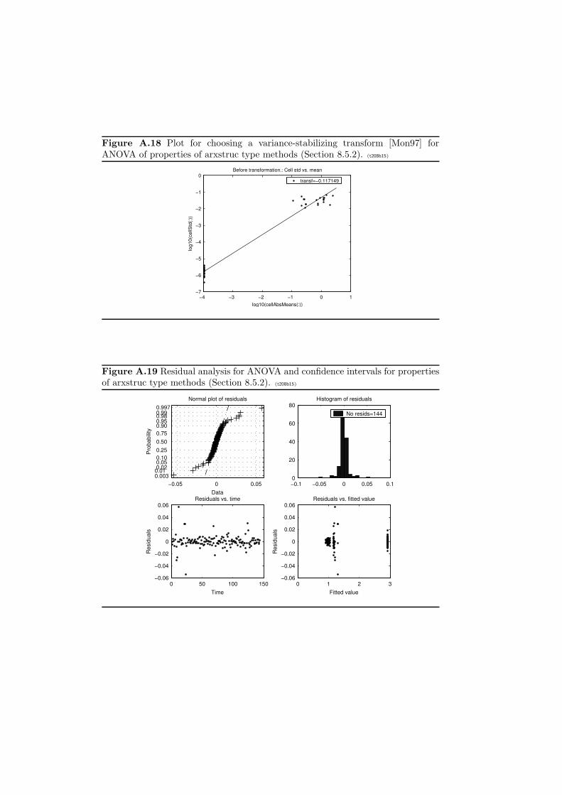
Figure A.18 Plot for choosing a variance-stabilizing transform [Mon97] forANOVA of properties of arxstruc type methods (Section 8.5.2). (t208b15)
−4 −3 −2 −1 0 1−7
−6
−5
−4
−3
−2
−1
0
log10(cellAbsMeans(:))
log1
0(ce
llStd
(:))
Before transformation.: Cell std vs. mean
transf=−0.117149
PSfrag replacements
tu(t)y(t)s(t)
gts(t)
TdTd
δ(t− Td)g(t)gr(t)g(t)
w(t)r(t)e(t)u(t)y(t)v(t)H(s)F (s)G(s)
Figure A.19 Residual analysis for ANOVA and confidence intervals for propertiesof arxstruc type methods (Section 8.5.2). (t208b15)
−0.05 0 0.050.0030.01 0.02 0.05 0.10 0.25 0.50 0.75 0.90 0.95 0.98 0.99 0.997
Data
Pro
babi
lity
Normal plot of residuals
−0.1 −0.05 0 0.05 0.10
20
40
60
80Histogram of residuals
No resids=144
0 50 100 150−0.06
−0.04
−0.02
0
0.02
0.04
0.06Residuals vs. time
Time
Res
idua
ls
0 1 2 3−0.06
−0.04
−0.02
0
0.02
0.04
0.06Residuals vs. fitted value
Fitted value
Res
idua
ls
PSfrag replacements
tu(t)y(t)s(t)
gts(t)
TdTd
δ(t− Td)g(t)gr(t)g(t)
w(t)r(t)e(t)u(t)y(t)v(t)H(s)F (s)G(s)
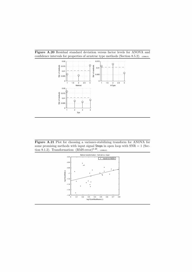
Figure A.20 Residual standard deviation versus factor levels for ANOVA andconfidence intervals for properties of arxstruc type methods (Section 8.5.2). (t208b15)
1 1.5 2 2.5 30
0.005
0.01
0.015
0.02
Method
Std
. of r
esid
uals
1 1.5 2 2.5 30
0.005
0.01
0.015
InType
Std
. of r
esid
uals
1 2 3 40
0.005
0.01
0.015
0.02
Sys
Std
. of r
esid
uals
PSfrag replacements
tu(t)y(t)s(t)
gts(t)
TdTd
δ(t− Td)g(t)gr(t)g(t)
w(t)r(t)e(t)u(t)y(t)v(t)H(s)F (s)G(s)
Figure A.21 Plot for choosing a variance-stabilizing transform for ANOVA forsome promising methods with input signal Steps in open loop with SNR = 1 (Sec-tion 9.1.2). Transformation: (RMS error)0.48. (t208b10)
0 0.1 0.2 0.3 0.4 0.5 0.6 0.7 0.8−1.8
−1.6
−1.4
−1.2
−1
−0.8
−0.6
−0.4
log10(cellAbsMeans(:))
log1
0(ce
llStd
(:))
Before transformation.: Cell std vs. mean
transf=0.478354
PSfrag replacements
tu(t)y(t)s(t)
gts(t)
TdTd
δ(t− Td)g(t)gr(t)g(t)
w(t)r(t)e(t)u(t)y(t)v(t)H(s)F (s)G(s)
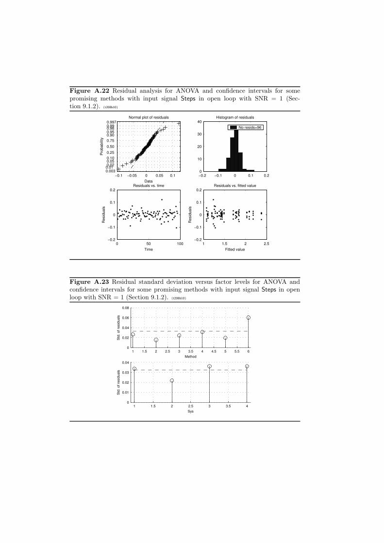
Figure A.22 Residual analysis for ANOVA and confidence intervals for somepromising methods with input signal Steps in open loop with SNR = 1 (Sec-tion 9.1.2). (t208b10)
−0.1 −0.05 0 0.05 0.10.0030.01 0.02 0.05 0.10 0.25
0.50
0.75 0.90 0.95 0.98 0.99 0.997
Data
Pro
babi
lity
Normal plot of residuals
−0.2 −0.1 0 0.1 0.20
10
20
30
40Histogram of residuals
No resids=96
0 50 100−0.2
−0.1
0
0.1
0.2Residuals vs. time
Time
Res
idua
ls
1 1.5 2 2.5−0.2
−0.1
0
0.1
0.2Residuals vs. fitted value
Fitted value
Res
idua
ls
PSfrag replacements
tu(t)y(t)s(t)
gts(t)
TdTd
δ(t− Td)g(t)gr(t)g(t)
w(t)r(t)e(t)u(t)y(t)v(t)H(s)F (s)G(s)
Figure A.23 Residual standard deviation versus factor levels for ANOVA andconfidence intervals for some promising methods with input signal Steps in openloop with SNR = 1 (Section 9.1.2). (t208b10)
1 1.5 2 2.5 3 3.5 4 4.5 5 5.5 60
0.02
0.04
0.06
0.08
Method
Std
. of r
esid
uals
1 1.5 2 2.5 3 3.5 40
0.01
0.02
0.03
0.04
Sys
Std
. of r
esid
uals
PSfrag replacements
tu(t)y(t)s(t)
gts(t)
TdTd
δ(t− Td)g(t)gr(t)g(t)
w(t)r(t)e(t)u(t)y(t)v(t)H(s)F (s)G(s)
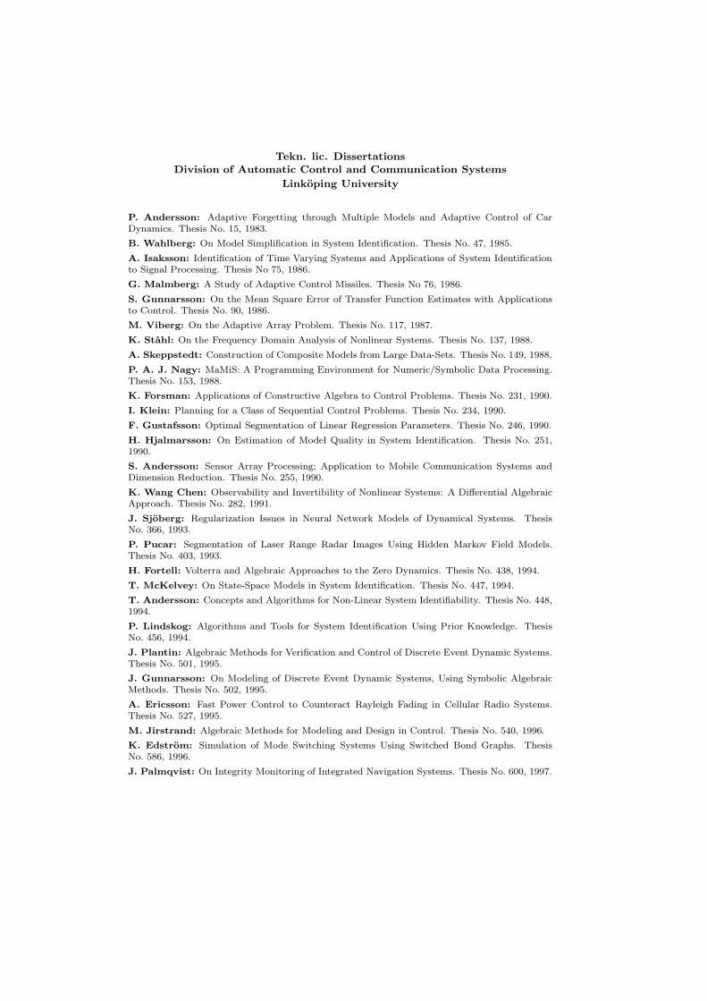
Tekn. lic. DissertationsDivision of Automatic Control and Communication Systems
Linkoping University
P. Andersson: Adaptive Forgetting through Multiple Models and Adaptive Control of CarDynamics. Thesis No. 15, 1983.
B. Wahlberg: On Model Simplification in System Identification. Thesis No. 47, 1985.
A. Isaksson: Identification of Time Varying Systems and Applications of System Identificationto Signal Processing. Thesis No 75, 1986.
G. Malmberg: A Study of Adaptive Control Missiles. Thesis No 76, 1986.
S. Gunnarsson: On the Mean Square Error of Transfer Function Estimates with Applicationsto Control. Thesis No. 90, 1986.
M. Viberg: On the Adaptive Array Problem. Thesis No. 117, 1987.
K. Stahl: On the Frequency Domain Analysis of Nonlinear Systems. Thesis No. 137, 1988.
A. Skeppstedt: Construction of Composite Models from Large Data-Sets. Thesis No. 149, 1988.
P. A. J. Nagy: MaMiS: A Programming Environment for Numeric/Symbolic Data Processing.Thesis No. 153, 1988.
K. Forsman: Applications of Constructive Algebra to Control Problems. Thesis No. 231, 1990.
I. Klein: Planning for a Class of Sequential Control Problems. Thesis No. 234, 1990.
F. Gustafsson: Optimal Segmentation of Linear Regression Parameters. Thesis No. 246, 1990.
H. Hjalmarsson: On Estimation of Model Quality in System Identification. Thesis No. 251,1990.
S. Andersson: Sensor Array Processing; Application to Mobile Communication Systems andDimension Reduction. Thesis No. 255, 1990.
K. Wang Chen: Observability and Invertibility of Nonlinear Systems: A Differential AlgebraicApproach. Thesis No. 282, 1991.
J. Sjoberg: Regularization Issues in Neural Network Models of Dynamical Systems. ThesisNo. 366, 1993.
P. Pucar: Segmentation of Laser Range Radar Images Using Hidden Markov Field Models.Thesis No. 403, 1993.
H. Fortell: Volterra and Algebraic Approaches to the Zero Dynamics. Thesis No. 438, 1994.
T. McKelvey: On State-Space Models in System Identification. Thesis No. 447, 1994.
T. Andersson: Concepts and Algorithms for Non-Linear System Identifiability. Thesis No. 448,1994.
P. Lindskog: Algorithms and Tools for System Identification Using Prior Knowledge. ThesisNo. 456, 1994.
J. Plantin: Algebraic Methods for Verification and Control of Discrete Event Dynamic Systems.Thesis No. 501, 1995.
J. Gunnarsson: On Modeling of Discrete Event Dynamic Systems, Using Symbolic AlgebraicMethods. Thesis No. 502, 1995.
A. Ericsson: Fast Power Control to Counteract Rayleigh Fading in Cellular Radio Systems.Thesis No. 527, 1995.
M. Jirstrand: Algebraic Methods for Modeling and Design in Control. Thesis No. 540, 1996.
K. Edstrom: Simulation of Mode Switching Systems Using Switched Bond Graphs. ThesisNo. 586, 1996.
J. Palmqvist: On Integrity Monitoring of Integrated Navigation Systems. Thesis No. 600, 1997.
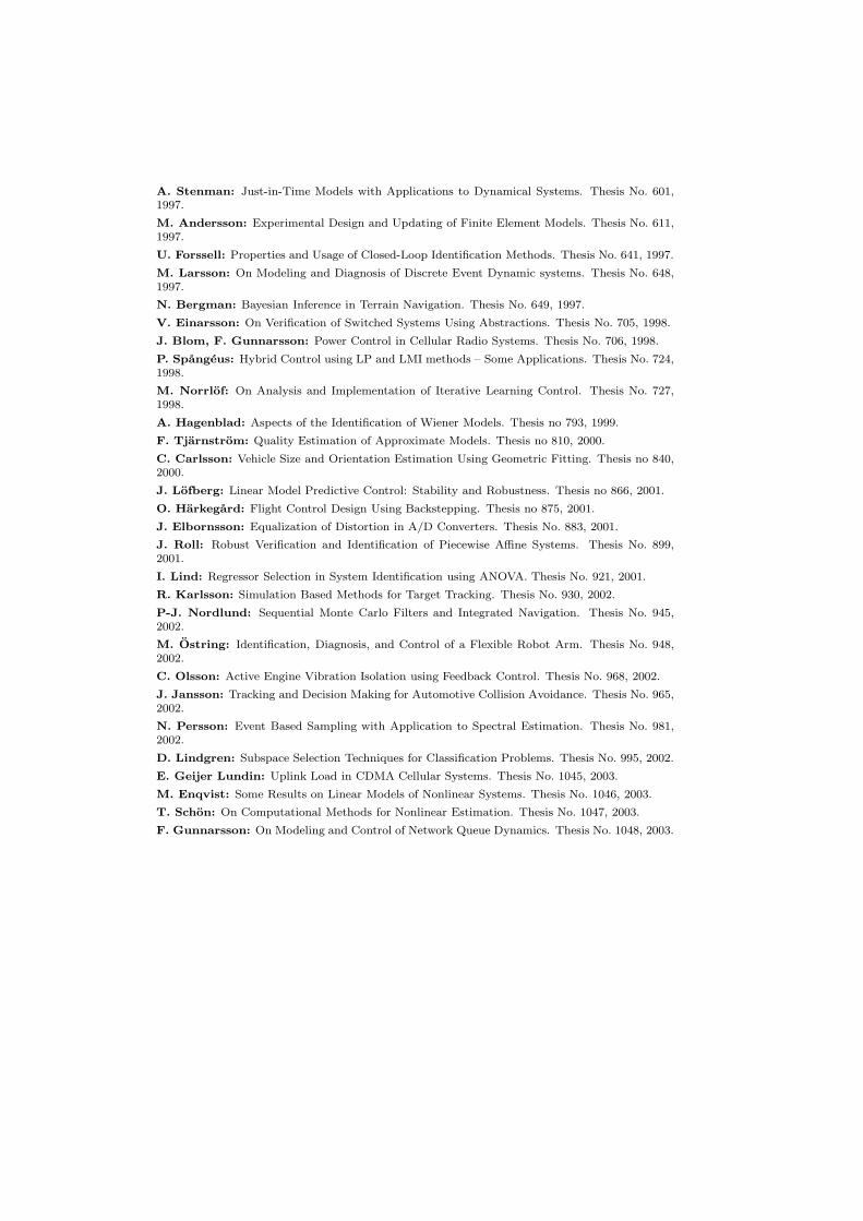
A. Stenman: Just-in-Time Models with Applications to Dynamical Systems. Thesis No. 601,1997.
M. Andersson: Experimental Design and Updating of Finite Element Models. Thesis No. 611,1997.
U. Forssell: Properties and Usage of Closed-Loop Identification Methods. Thesis No. 641, 1997.
M. Larsson: On Modeling and Diagnosis of Discrete Event Dynamic systems. Thesis No. 648,1997.
N. Bergman: Bayesian Inference in Terrain Navigation. Thesis No. 649, 1997.
V. Einarsson: On Verification of Switched Systems Using Abstractions. Thesis No. 705, 1998.
J. Blom, F. Gunnarsson: Power Control in Cellular Radio Systems. Thesis No. 706, 1998.
P. Spangeus: Hybrid Control using LP and LMI methods – Some Applications. Thesis No. 724,1998.
M. Norrlof: On Analysis and Implementation of Iterative Learning Control. Thesis No. 727,1998.
A. Hagenblad: Aspects of the Identification of Wiener Models. Thesis no 793, 1999.
F. Tjarnstrom: Quality Estimation of Approximate Models. Thesis no 810, 2000.
C. Carlsson: Vehicle Size and Orientation Estimation Using Geometric Fitting. Thesis no 840,2000.
J. Lofberg: Linear Model Predictive Control: Stability and Robustness. Thesis no 866, 2001.
O. Harkegard: Flight Control Design Using Backstepping. Thesis no 875, 2001.
J. Elbornsson: Equalization of Distortion in A/D Converters. Thesis No. 883, 2001.
J. Roll: Robust Verification and Identification of Piecewise Affine Systems. Thesis No. 899,2001.
I. Lind: Regressor Selection in System Identification using ANOVA. Thesis No. 921, 2001.
R. Karlsson: Simulation Based Methods for Target Tracking. Thesis No. 930, 2002.
P-J. Nordlund: Sequential Monte Carlo Filters and Integrated Navigation. Thesis No. 945,2002.
M. Ostring: Identification, Diagnosis, and Control of a Flexible Robot Arm. Thesis No. 948,2002.
C. Olsson: Active Engine Vibration Isolation using Feedback Control. Thesis No. 968, 2002.
J. Jansson: Tracking and Decision Making for Automotive Collision Avoidance. Thesis No. 965,2002.
N. Persson: Event Based Sampling with Application to Spectral Estimation. Thesis No. 981,2002.
D. Lindgren: Subspace Selection Techniques for Classification Problems. Thesis No. 995, 2002.
E. Geijer Lundin: Uplink Load in CDMA Cellular Systems. Thesis No. 1045, 2003.
M. Enqvist: Some Results on Linear Models of Nonlinear Systems. Thesis No. 1046, 2003.
T. Schon: On Computational Methods for Nonlinear Estimation. Thesis No. 1047, 2003.
F. Gunnarsson: On Modeling and Control of Network Queue Dynamics. Thesis No. 1048, 2003.